This is a repository copy of Memory, expectation formation and scheduling choices.

White Rose Research Online URL for this paper:http://eprints.whiterose.ac.uk/90836/

Version: Accepted Version

Article:

Koster, P, Peer, S and Dekker, T (2015) Memory, expectation formation and scheduling choices. Economics of Transportation, 4 (4). pp. 256-265. ISSN 2212-0122

https://doi.org/10.1016/j.ecotra.2015.09.001

© 2015, Elsevier. Licensed under the Creative Commons Attribution-NonCommercial-NoDerivatives 4.0 International http://creativecommons.org/licenses/by-nc-nd/4.0/

eprints@whiterose.ac.ukhttps://eprints.whiterose.ac.uk/

Reuse

Unless indicated otherwise, fulltext items are protected by copyright with all rights reserved. The copyright exception in section 29 of the Copyright, Designs and Patents Act 1988 allows the making of a single copy solely for the purpose of non-commercial research or private study within the limits of fair dealing. The publisher or other rights-holder may allow further reproduction and re-use of this version - refer to the White Rose Research Online record for this item. Where records identify the publisher as the copyright holder, users can verify any specific terms of use on the publisher’s website.

Takedown

If you consider content in White Rose Research Online to be in breach of UK law, please notify us by emailing eprints@whiterose.ac.uk including the URL of the record and the reason for the withdrawal request.

Memory, expectation formation and scheduling choicesI

Paul Kostera,b,∗, Stefanie Peerc, Thijs Dekkerd

aDepartment of Spatial Economics, VU University Amsterdam, De Boelelaan 1105,

1081 HV Amsterdam, The NetherlandsbTinbergen Institute, Gustav Mahlerplein 117, 1082 MS Amsterdam, The Netherlands

cVienna University of Business and Economics, Welthandelsplatz 1, 1020 Vienna, AustriadUniversity of Leeds, Institute for Transport Studies, 36-40 University Road, Leeds, LS2 9JT, UK.

Abstract

Limited memory capacity, retrieval constraints and anchoring are central to expectation for-mation processes. We develop a model of adaptive expectations where individuals are ableto store only a finite number of past experiences of a stochastic state variable. Retrieval ofthese experiences is probabilistic and subject to error. We apply the model to schedulingchoices of commuters and demonstrate that memory constraints lead to sub-optimal choices.We analytically and numerically show how memory-based adaptive expectations may sub-stantially increase commuters’ willingness-to-pay for reductions in travel time variability,relative to the rational expectations outcome.

Article published as: Koster, P., Peer, S. and Dekker,T. (2015). Memory, expectationformation and scheduling choices. Economics of Transportation.http://dx.doi.org/10.1016/j.ecotra.2015.09.001

Keywords: Memory, Transience, Expectation formation, Adaptive expectations, RetrievalAccuracy, Scheduling, Value of Reliability

IWe like to thank two anonymous referees for very helpful suggestions for improvements. The paper alsobenefited from suggestions and comments of Alexander Muermann, Hans Koster, Peter Nijkamp, participantsof the 2014 conference of the European Association for Research in Transportation (hEART) in Leeds,participants of the 2014 conference of the International Transportation Economic Association (ITEA) inToulouse, participants of a TLO seminar at Delft University. Paul Koster gratefully acknowledges thefinancial support of the ERC (Advanced Grant OPTION # 246969).

∗Corresponding author. Fax +31 20 5986004, phone +31 20 5984847.Email addresses: p.r.koster@vu.nl (Paul Koster), speer@wu.ac.at (Stefanie Peer),

t.dekker@leeds.ac.uk (Thijs Dekker)

1

1. Introduction

Imperfect knowledge regarding the true distribution of stochastic state variables, like prod-uct quality or travel times, induces individuals to form expectations based on personalexperiences and external sources of information. Memory processes are known to influenceexpectation formation processes (e.g. Hirshleifer and Welch, 2002; Mullainathan, 2002; Wil-son, 2003; Sarafidis, 2007) and anchoring constitutes a persistent phenomenon in humanbehaviour (Wilson et al., 1996; Strack and Mussweiler, 1997; Furnham and Boo, 2011).1

This paper develops an adaptive expectations model which explicitly accounts for limitedcognitive abilities of decision makers. Expectation formation in our model has the followingproperties. First, decision makers are assumed to have limited memory, such that only a fixednumber of past experiences can be stored. Second, retrieving experiences from memory isprobabilistic and decision makers experience difficulty in retrieving more distant experiences;a phenomenon often referred to as transience (Horowitz, 1984; Barucci, 1999, 2000; Schacter,2002). Third, retrieval may be inaccurate, meaning that retrieved experiences may notcorrespond to the original experiences. Transience and retrieval inaccuracy are both formsof memory decay. Fourth, decision makers prime their expectations using exogenous anchors.The inclusion of past experiences, limited cognitive abilities and anchoring in the expectationformation model provides a significant deviation of the rational expectations model.

We apply the model to scheduling decisions of commuters facing stochastic daily traveltimes. Commuters experience dis-utility from travel time variability, as it induces themto depart and/or arrive earlier or later than preferred (e.g. Vickrey, 1969; Small, 1982,1992; Noland and Small, 1995). The developed model provides a better understanding ofempirical findings that hint at the presence of adaptive expectations and anchors in thecontext of travel related scheduling decisions. For example, Bogers et al. (2007) and Ben-Elia and Shiftan (2010) provide evidence that recently experienced travel times have an over-proportionally large influence on travel decisions. Peer et al. (2015) find that commuterstake into account the long-run travel time average as well as day-specific traffic informationin their scheduling decisions.

The value commuters attach to a marginal reduction in travel time variability is referredto as the value of (travel time) reliability and can be inferred from observed schedulingchoices (Fosgerau and Karlstrom, 2010; Fosgerau and Engelson, 2011). Typically, the valueof reliability is derived using the presumption that commuters have rational expectationsand an infinite memory. We find that with adaptive travel time expectations this valueof reliability is higher, because sub-optimal scheduling decisions are made. Therefore, im-provements in reliability are associated with larger benefits, because they make commutersdepart and arrive closer to the times they prefer and decrease the variability in departuretimes. Empirical revealed preference studies using reduced-form utility functions are likelyto already capture these behavioural biases in the coefficient that is estimated for travel

1Often anchors corresponds to the information that is obtained first, which is then used as a referencepoint in subsequent decisions (Tversky and Kahneman, 1974). Ariely et al. (2003), for instance, demon-strated that individuals can be primed to anchors that are as random as the last two digits of their socialsecurity number.

2

time variation. Our results are therefore mainly important for current stated preferencepractice that ignores the process of expectation formation: our numerical illustration showsthat these values of reliability can underestimate our bounded rationality value of reliabilityby up to 45%, suggesting that the welfare effects of memory biases may be substantial.

Underestimation of the value of reliability may have significant implications for cost-benefit assessments of transport policies. Namely, the benefits from improvements in traveltime reliability in road-related transport projects amount to ca. 25% of the benefits relatedto travel time gains (Peer et al., 2012). Benefits from travel time gains, in turn, are estimatedto constitute on average 60% of total user benefits in transport appraisals (Hensher, 2001).

While we apply our model to scheduling choices of commuters, it may very well berelevant to other fields of economics, such as for the study of the effects of heterogeneous ex-pectation formation on (dis)equilibrium in dynamic economic systems (see Hommes (2013))or for the analysis of repetitive consumer choices with uncertain product quality. Note thatbounded rationality in our model is exclusively caused by limited cognitive abilities ratherthan judgement errors due to selective memory (Gennaioli and Shleifer, 2010) or probabilityweighting. Therefore this paper stands apart from works modelling bounded rationality asa result of satisficing (Simon, 1955; Caplin et al., 2011), self-deception (Benabou and Ti-role, 2002), or optimal belief formation when the decision utility is affected by anticipatoryemotions (Brunnermeier and Parker, 2005; Bernheim and Thomadsen, 2005) as well as by(ex-post) disappointment (Gollier and Muermann, 2010).

The remainder of the paper is structured as follows. Section 2 describes the generalsetup of the model, Section 3 applies that model to the specific case of scheduling decisions.Section 4 provides numerical estimates of the biases that may result from memory limitationsand anchoring. Finally, Section 5 discusses the modelling assumptions and concludes.

2. General description of the model

Consider a decision-maker who decides on x0, where the subscript 0 indicates that thedecision is made for the time period to come. Outcome utility U(x0, s0) is assumed to becontinuous and strictly concave in x0, and depends on the stochastic state s0. Let f(s0|ω0) bethe probability density function of s0, where ω0 is a vector of parameters that characterizesf(.). Expected outcome utility is then defined as:

E(U(x0, s0)) =

∫

U(x0, s0)f(s0|ω0)ds0 (1)

With rational expectations, the decision maker knows the distribution f(s0|ω0) and maxi-mizes Equation 1 to decide on x0. In what follows, we denote xre

0 as the optimal choice underrational expectations, and E(Ure) ≡ E(U(xre

0 , s0)) as the corresponding maximal expectedutility. Deviations from rational expectations are introduced by assuming that the decisionmaker has imperfect knowledge regarding f(s0|ω0). In our model, she forms adaptive ex-pectations regarding s0, using past experiences in combination with primed expectations.Past experiences are denoted by past stochastic realisations of sk, which are draws from

3

f(sk|ωk). A higher value of the index k refers to a more distant experience. Primed expec-tations enter the model in the form of an anchor state sA. In contrast to the states storedin the decision maker’s memory and the corresponding retrievals, the anchor is assumed tobe non-stochastic and is a stable element in the expectation formation process.

The decision maker is assumed to have limited cognitive abilities. First, it is assumedthat she has a limited memory, meaning that only K past experiences s1...sK are storedin memory. Second, it is assumed that the realisation of sk is correctly stored in memory,but a stored state can only be retrieved with a probability ρk > 0. Following Schacter(2002), this allows us to assume that more recent experiences can be retrieved more easily,i.e. ρ1 > ρ2 > ... > ρK . We refer to this phenomena as transience. Third, retrieval ofthe stored states s1...sK may be inaccurate. Instead of s1...sK , the decision maker retrievess1...sK from her memory. Let gk (sk|sk, φk) be the retrieval density function, with φk andsk as its characterizing parameters. Fourth, anchoring is present. The anchor reflects anexogenous, stable belief concerning travel time that is independent of new experiences andthe current traffic situation. While we do not model the origin of the anchor explicitly inorder to keep the model generic, the anchor could for example be driven by stable publiclyavailable information.

Equation 2 defines the expected decision utility as the weighted average of utilities acrossthe anchor and the set of retrieved states:

Ud(.) = τU(x0, sA) + (1− τ)K∑

k=1

ρkU(x0, sk), (2)

where∑K

k=1 ρk = 1. In this equation, τ is the weight assigned to the anchor. When τ = 0,expectations are fully adaptive and when τ = 1, the decision maker ignores her earlierexperiences and expected decision utility is solely based on the anchor sA and the choice ofx0. Equation 2 mimics Equation 1 when τ → 0, ρk = 1/K, sk = sk and K → ∞. Rationalexpectations are therefore a special case of our model. The decision maker maximizesEquation 2 with respect to x0. Denote this optimal x0 by xae

0 , where the ae superscriptrefers to the fact that the decision maker uses adaptive expectations.2 Decisions on x0 aresub-optimal whenever xae

0 6= xre0 . Nevertheless, the situation could arise where xae

0 = xre0 ,

i.e. the decision maker ’coincidentally’ makes the optimal choice.Suppose that we need to make a prediction of the expected outcome utility of the decision

maker. This prediction has to account for the fact that the state in time period 0, the statesin memory and the corresponding retrievals of these states are stochastic. To obtain thepredicted expected outcome utility, we take the expected value over all possible combinationsof experienced and retrieved states. Mathematically this is tedious, since it involves a 2K+1dimensional integral over all possible values of the K + 1 realised states s0...sK , and the K

2A unique solution for xae0 exists since Equation 2 is a weighted average of strictly concave functions.

4

possible values of retrieved states s1...sK :

E(Uae) ≡ E (U(xae0 , s0))

=

∫

...

∫

(

∫

...

∫

U(xae0 , s0)

K∏

k=1

gk (sk|sk, φk) ds1...sK)

)

K∏

k=0

f(sk, ωk)ds0...dsK .(3)

This equation obviously has the disadvantage that it is less parsimonious than its rationalexpectations counterpart, i.e. Equation 1 with xre

0 . Nevertheless, this generic set-up helps tostructure our thoughts about how earlier experiences and retrieval inaccuracy affect predic-tions of the expected outcome utility. The next section makes analytical progress by puttingmore structure on the utility function U(.) and derives an analytical representation of thepredicted expected outcome utility E(Uae) for the case of commuters choosing departuretimes when travel times are stochastic.

3. Memory and the value of travel time reliability

We apply our memory-based adaptive expectation formation model to commuters’ schedul-ing behaviour with stochastic travel times. Commuters face scheduling costs of travel timevariability due to departing and/or arriving earlier or later than desired. Noland and Small(1995) were the first to extend the scheduling model of Vickrey (1969) and Small (1982) toexpected utility maximization. Their model was recently extended by Fosgerau and Karl-strom (2010) and Fosgerau and Engelson (2011) who proved that the optimal expectedoutcome utility depends linearly on some measure of travel time reliability. Here, we ex-tend the results of Fosgerau and Engelson (2011) by showing that this result carries over tothe case when memory biases and anchoring are present and the travel time distribution isstable over time. Existing literature on travel time expectation formation typically focuseson learning and perception updating mechanisms in route choice but often ignores the psy-chological foundation of the adaptation of expectations (e.g. Jha et al., 1998; Arentze andTimmermans, 2003; Chen and Mahmassani, 2004; Avineri and Prashker, 2005; Arentze andTimmermans, 2005; Bogers et al., 2007; Ben-Elia and Shiftan, 2010). Moreover, most exist-ing studies do not quantify behavioural and valuation biases, even when they find that traveltime expectations are adaptive. Therefore it is unclear if choice models assuming rationalexpectations can be viewed as a good approximation of individual choice behaviour. Thispaper explicitly focuses on the origins of adaptive travel time expectations and characterizesthe resulting behavioural and valuation biases.

3.1. Rational expectations

We assume commuters derive utility from being at home, for instance by spending moretime with the family, sleeping or having a longer breakfast. Departing earlier or later thanpreferred therefore reduces utility. Similarly, utility at work is derived from productive worktime, which is reduced by arriving later than preferred. An increase in travel time thereforereduces utility on either end. This specification of utility was first introduced by Vickrey(1973) and later used by Fosgerau and Engelson (2011) to derive the value of reductions in

5

travel time variance. Tseng and Verhoef (2008) were the first to find empirical evidence forsuch scheduling preferences.Equation 4 describes outcome utility for a given departure time d0 and a realisation of traveltime T0, where H ′(v) is the marginal utility for being at home and W ′(v) is the marginalutility for being at work as functions of clock time v. The first part of Equation 4 showsthe utility from time spent at home where being at home starts at vh and ends when thetravellers departs at d0. The second integral gives the utility for being at work, where beingat work starts at arrival time d0 + T0 and ends at vw. This implies that vh and vm span therange of possible departure and arrival times (Borjesson et al. (2012)).3

V (d0|T0) =

∫ d0

vh

H ′(v)dv +

∫ vw

d0+T0

W ′(v)dv = H(d0)−H(vh) +W (vw)−W (d0 + T0). (4)

For the remainder of the paper we assume simple linear functional forms for the marginalutilities. Using the normalisation of Borjesson et al. (2012) we have:4

U(d0|T0) = −

∫ 0

d0

(β0 + β1v)dv −

∫ d0+T0

0

(β0 + γ1v)dv. (5)

For a trip to occur it must hold that γ1 > β1. Usually the marginal utility of being athome is decreasing in v, implying β1 < 0, whereas the marginal utility of being at work isincreasing (γ1 > 0). With rational expectations, commuters know the distribution of traveltimes which is defined by f(T0|µ, σ

2), where µ is the mean travel time and σ2 the travel timevariance. Accordingly, the expected outcome utility is defined by:

E(U(d0|T0)) =

∫

U(d0|T0)f(T0|µ, σ2)dT0. (6)

Fosgerau and Engelson (2011) show that when the departure time is optimally chosen, thecommuter departs at:

dre0 = −γ1

γ1 − β1

µ, (7)

resulting in optimal expected outcome utility:

E(Ure) ≡ E(U(dre0 |T0)) = −β0µ+1

2

β1γ1γ1 − β1

µ2 −1

2γ1σ

2. (8)

3For a graphical representation we refer to Tseng and Verhoef (2008), Fosgerau and Engelson (2011)and Borjesson et al. (2012).

4Following Borjesson et al. (2012), we normalise utility relative to V (0|0), by defining U(d0|T0) =V (d0|T0)− V (0|0). This allows us to evaluate U(d0|T0) in terms of bounds at 0 rather than at vh and vm:

U(d0|T0) = −

∫ 0

d0

H ′(v)dv −

∫ d0+T0

0

W ′(v)dv = H(d0)−H(0) +W (0)−W (d0 + T0)

Furthermore, we normalise W (0)−H(0) to 0, because this part of utility is independent of departure timed0 and travel time T0. We do so by assuming that H ′(v) and W ′(v) have the same intercept.

6

This optimal expected outcome utility is a simple function of the mean delay and the traveltime variance. Equation 8 does not require any distributional assumptions on the traveltime distribution (except that µ and σ2 are finite). We define the value of reliability (VOR)as the value attached to a marginal decrease in the travel time variance:5

VORre = −∂E(Ure)

∂σ2=

1

2γ1. (9)

3.2. Adaptive expectations

Adaptive expectations on the distribution of travel times are based on past travel timesstored in memory T1...TK and the retrievals of these past states T1...TK . Every retrievalis assumed to be an additive function of the retrieval error and the realised travel time:Tk = Tk + ǫk, with E(ǫk) = 0, meaning that retrieval is on average correct. The travel timesin memory are realizations from f(Tk|µ, σ

2). The accuracy of retrieval ǫk is governed bythe probability density function g(Tk|Tk, ν

2k) where Tk has mean E(Tk) = Tk and conditional

variance VAR(Tk|Tk) = ν2k . Using the law of total variance, the unconditional variance

of Tk is given by: VAR(Tk) = σ2 + ν2k .

6 For every day t the commuter has to decideon the departure time and creates a new set of recalled memories from the stored set ofpast experiences. For large K, the set of past travel time experiences stored in memoryfor days t and t + 1 is nearly identical as the experienced travel time at t only replacesa single experience previously stored in memory. The similarity in available memories incombination with transience introduces correlation in the recalled sets, but the process ofthe recollection and accuracy of these recollections are completely independent between tand t+ 1.

The commuter has an anchor TA which is defined as: TA = µ + a, where a is a pa-rameter that indicates how far the anchor is from the mean travel time µ. With adaptiveexpectations, commuters choose their optimal departure using decision utility

Ud(.) = τU(d0, TA) + (1− τ)K∑

k=1

ρkU(d0, Tk), (10)

where∑K

k=1 ρk = 1. Solving the first-order condition ∂Ud(.)∂d0

= 0 gives:

dae0 = −τγ1

γ1 − β1

TA − (1− τ)γ1

γ1 − β1

K∑

k=1

ρkTk. (11)

5For plausibility of the model, additional restrictions may be imposed because for some combinationsof preference parameters the marginal utility for changes in the mean delay −β0 +

β1γ1

γ1−β1

µ may be positive,implying that increases in mean travel time would lead to a higher expected utility.

6 We assume COV(Tk, Tl) = 0, COV(Tk, ǫl) = 0, and COV(ǫk, ǫl) = 0, ∀k 6= l. Together with theassumption that E(ǫk) = 0, ∀k, this results in COV(Tk, Tl) = E(TkTl)− E(Tk)E(Tl) = E(TkTl) + E(Tkǫl) +E(Tlǫk) + E(ǫkǫl)− E(Tk)E(Tl) = 0, ∀k 6= l. Relaxing these assumptions is an interesting avenue for futureresearch.

7

The effect of the anchor on departure time choice is captured by the first term, and theeffect of limited memory by the second term. A higher K indicates that the commuter isable to store more past travel times. Stored travel times are retrieved with probability ρk.Retrieval accuracy enters the departure time choice via the retrieved travel times Tk. Themean departure time is given by:

E (dae0 ) = −τγ1

γ1 − β1

TA − (1− τ)γ1

γ1 − β1

µ, (12)

which reduces to dre0 for TA = µ (a = 0) (see Equation 7). The variability in departuretime choices over time periods is influenced by the variance of travel times and the varianceof retrieval inaccuracy. A higher variance in travel times and a higher retrieval inaccuracyresult in more variable departure times:7

VAR(dae0 ) = (1− τ)2(

γ1γ1 − β1

)2(

σ2

K∑

k=1

ρ2k +K∑

k=1

ρ2kν2k

)

. (13)

Our model therefore predicts that the variability in departure times increases for increasingvariances of travel time and retrieval. This effect is multiplied with the quadratic retrievalprobabilities. When transience is stronger, retrieval probabilities will be more unequal,resulting in more volatile behaviour. A higher anchor parameter τ results in less variabledeparture times because memory biases count less heavily in the decision utility function.The prediction of the expected outcome utility can be found by integrating over all possiblecombinations of T0, T1...TK and the corresponding stochastic retrievals T1...TK (i.e. in asimilar way as Equation 3). In Appendix A we show that the predicted expected outcomeutility E(Uae) can be written as:8

E(Uae) = E(Ure)−1

2

γ21

γ1 − β1

τ 2a2 −1

2(γ1 − β1)VAR(d

ae0 )

= E(Ure)−1

2

γ21

γ1 − β1

τ 2a2 −1

2(1− τ)2

γ21

γ1 − β1

(

σ2

K∑

k=1

ρ2k +K∑

k=1

ρ2kν2k

)

.

(14)

The first term in Equation 14 is the optimal expected utility with rational expectations(Equation 8). The second term reflects a penalty for relying on an anchor when deciding onthe optimal departure time. This penalty only arises when a 6= 0, and increases quadrati-cally in the value of a and the anchor parameter τ . When τ → 1 and TA = µ, the optimaldeparture time Equation 11 is equal to the departure time with rational expectations andEquation 14 reduces to Equation 8.

7Here we use the assumptions on covariances in footnote 6. When relaxing these assumption additionalcovariance terms would enter this equation.

8The model developed in Appendix A is more general because it assumes a k-specific travel time distri-bution. We leave this out in the discussion because it gives rise to another type of memory bias related tovariations of travel time distributions over subsequent days.

8

Adaptive expectations are associated with an additional term that is proportionally decreas-ing in the variance of departure time VAR(dae0 ). More volatile behaviour therefore decreasesthe predicted expected outcome utility. First, an increase in the travel time variance resultsin additional dis-utility because of limited memory. Second, K enters the summation overall retrieval variances νk. Accordingly, the retrieval variances of the last K time periodsdecrease expected outcome utility. The negative effect of transience and inaccurate retrievalbecomes stronger when commuters’ expectations become more adaptive (i.e. when τ de-creases).Equation 14 is derived for general values of retrieval probabilities, travel time variance andretrieval variances. When imposing transience, we have ρ1 > ρ2 > ... > ρK , such that morerecent travel time and retrieval variances play a larger role than more distant travel timeand retrieval variances in Equation 14. Because retrieval probabilities enter quadratically,transience always reduces utility when retrieval is accurate. However, when retrieval vari-ances are high for more distant memories (i.e. higher values of k), transience may reducethe bias of inaccurate retrieval.The anchor parameter τ has two roles in Equation 14. Given TA 6= µ, an increase in τ isassociated with a decrease in expected utility due to the sub-optimal choice of TA. On theother hand, an increase in τ may lead to a decrease in the bias related to transience andretrieval inaccuracy, since past experiences have a lower effect on travel time expectations.

3.3. The value of travel time reliability

The VOR with adaptive expectation is given by:

VORae = −∂E(Uae)

∂σ2=

1

2γ1 +

1

2

γ21

γ1 − β1

(1− τ)2K∑

k=1

ρ2k, (15)

where it is assumed that τ is exogenous. As with rational expectations (see 9), the expectedoutcome utility is linearly decreasing in the travel time variance. The convenient result ofFosgerau and Engelson (2011) thus carries over to the case of adaptive expectations. Whilethe VOR is not affected by retrieval inaccuracy, it is affected by transience and the anchorweight τ . Regarding τ , it is easy to see that the VOR increases as the weight attached to theanchor decreases and expectations thus become more adaptive. Clearly, if τ → 1 (and henceonly the anchor counts), the VOR is not any longer affected by the transience parameter ρk.

It is useful to parametrize the retrieval probabilities. These probabilities need to sum upto 1 for any chosen value of K = 1...∞, and for transience to apply, the probabilities needto be decreasing in k, because more recent travel times will then have a higher likelihood ofbeing remembered. A functional form that satisfies these conditions is given by:

ρk =r − 1

r(rK − 1)rk, (16)

where 0 < r < 1. In this equation, the parameter r is the transience parameter. A lowervalue of r indicates more transience, meaning that more recent travel times receive a higherretrieval probability. An increase in r results in more equal weights where equal weights

9

1K

are a limiting case, because limr→1 ρk = 1K. If we assume that retrieval probabilities are

defined by Equation 16, the VORae is given by:

VORae,r =1

2γ1 +

1

2

γ21

γ1 − β1

(1− τ)2(1− r)(1 + rK)

(1 + r)(1− rK), (17)

which is decreasing in the transience parameter r, meaning that more unequal retrievalprobabilities increase the value attached to reliable travel times. The limiting case r → 1gives retrieval probabilities equal to 1/K. The value of travel time variance is then given by

limr→1

VORae,r =1

2γ1 +

1

2

γ21

γ1 − β1

(1− τ)21

K, (18)

and therefore in the absence of transience the additional effect of limited memory on theVORae is proportional to

1K. As expected, the behavioural bias due to limited memory then

vanishes when K → ∞, and VORae,r reduces to 9.

3.4. The value of retrieval accuracy

The expected outcome utility (see Equation 14) shows that it is valuable for commuters tohave a higher accuracy of retrieval. The value of retrieval accuracy (VORA) for retrieval mis defined as the first derivative of Equation 14 with respect to ν2

m, multiplied by (−1):

VORAm = −∂E(Uae)

∂ν2m

=1

2

γ21

γ1 − β1

(1− τ)2ρ2m, ∀m = 1...K. (19)

The VORA increases when expectations become more adaptive (τ → 0), and when thatparticular experience has a larger impact on the expected outcome utility. A more explicitexpression can be derived by replacing ρm in Equation 19 by Equation 16:

VORAm,r =1

2

γ21

γ1 − β1

(1− τ)2(

r − 1

r(rK − 1)rm)2

, ∀m = 1...K. (20)

In line with intuition, when transience is present, the VORA is lower for more distantmemories (higher m). This illustrates the interesting interplay between transience and theeffects of retrieval inaccuracy.

3.5. The limiting case of K → ∞ and ν2k → νk

This subsection develops a limiting case that may be useful for practical applications. It isassumed that memory is unlimited and that an infinite number of experiences are stored.Furthermore, it is assumed that the retrieval variance is linearly increasing in k with slopeν:

ν2k = νk. (21)

10

If we substitute Equations 16 and 21 in Equation 14 we obtain a parsimonious expression forthe expected outcome utility under infinite memory as a function of the transience parameterr and retrieval variance parameter ν9:

E(Uae) = E(Ure)−1

2

γ21

γ1 − β1

τ 2a2 −1

2

γ21

γ1 − β1

(1− τ)21− r

1 + rσ2

−1

2

γ21

γ1 − β1

(1− τ)2ν

(1 + r)2.

(22)

The biases due to transience and inaccurate recall do not vanish when memory capacityis unlimited. Equation 22 does show that when the retrieval probabilities are all equal(r → 1), the third term drops out, and the transience bias vanishes, but the bias due toretrieval inaccuracy does not. Accordingly, infinite memory is not a sufficient assumptionfor rational expectations.

3.6. Endogenous choice of τ

This section generalizes the model to allow for the choice of the anchor parameter, whichcorresponds to the situation where the decision-maker is aware of her memory limitations.For a 6= 0, the decision-maker will trade-off the bias related to the anchor with the memorybiases. The change in expected utility for a marginal change in τ is given by:

∂E(Uae)

∂τ= −

γ21

γ1 − β1

τa2 +γ21

γ1 − β1

(1− τ)

(

σ2

K∑

k=1

ρ2k +K∑

k=1

ρ2kν2k

)

. (23)

Solving the first-order condition ∂E(Uae)∂τ

= 0 results in:

τ ∗ =

∑K

k=1 ρ2kσ

2 +∑K

k=1 ρ2kν

2k

∑K

k=1 ρ2kσ

2 +∑K

k=1 ρ2kν

2k + a2

(24)

which is equal to 1 if a = 0, and independent of scheduling preferences. The optimal anchorparameter weighs the dis-utility related to imprecision due to anchoring with the dis-utilityrelated to memory biases. Incorporating an anchor (i.e. τ ∗ 6= 0) is therefore a rationalresponse to cope with imprecision in knowledge about the true distribution. An increase inσ2 will result in an increase in τ ∗, because – as a consequence of the severity of the memorybiases – the decision-maker will rely more on her anchor:

∂τ ∗

∂σ2=

a2∑K

k=1 ρ2k

(

∑K

k=1 ρ2kσ

2 +∑K

k=1 ρ2kν

2k + a2

)2 > 0. (25)

9For the limiting case of K → ∞ we have:∑

∞

k=1 ρ2k = 1−r

1+r and∑

∞

k=1 ρ2kνk = ν

(1+r)2 , resulting in a

retrieval inaccuracy bias that is increasing in r. When retrieval inaccuracy increases more rapidly in k, theutilitarian bias resulting from retrieval inaccuracy might be decreasing in r.

11

A marginal upward change in τ ∗ results in a higher bias due to anchoring and a lower biasdue to transience and retrieval inaccuracy. In Appendix B we show that these marginalchanges cancel each other out, resulting in a value of reliability of:

VORae,τ∗ =1

2γ1 +

1

2

γ21

γ1 − β1

(1− τ ∗)2K∑

k=1

ρ2k

=1

2γ1 +

1

2

γ21

γ1 − β1

a4∑K

k=1 ρ2k

(

σ2∑K

k=1 ρ2k +

∑K

k=1 ρ2kν

2k + a2

)2 .

(26)

The last step uses Equation 24. The second positive term captures the combined dis-utilityfor anchoring and memory biases (i.e. transience and retrieval inaccuracy). For a = 0, theVOR reduces to the rational expectations case of Equation 9 because the decision-makerthen fully relies on the anchor (see Equation 24). This results in a departure time choicethat coincides with the rational expectations case (see Equations 7 and 11). The VOR isnow decreasing in the travel time variance, because the second term is lower for higher valuesof σ2. The convenient result that expected utility is linear in travel time variance thereforedoes not hold any longer when the anchor parameter is endogenous.

4. Numerical illustration

This section provides a numerical illustration to investigate the quantitative impact of mem-ory biases. We present results for four parameters, namely r, τ, TA, and ν, and trace theirimpacts on optimal departure times, expected utility and the value of travel time reliability.The rational expectation levels of these measures (as defined in Section 4.1) are used as thepoint of reference. Section 4.2 analyses the effect of transience by reducing the value of rsuch that expectations are increasingly based on recent experiences. At this stage, retrievalis assumed to be accurate. Section 4.3 maintains this assumption but introduces anchoringby increasing the value of τ and varying the value TA = µ + a. Section 4.4 completes thenumerical analysis by introducing inaccurate retrieval. Finally, Section 4.5 summarizes theresults of the numerical analysis.

4.1. Parameter assumptions and the rational expectations outcome

The values for the coefficients defining the rational expectations outcomes of the model arebased on Tseng and Verhoef (2008) and Fosgerau and Lindsey (2013). Accordingly, β0, β1

and γ1 take the following values: β0 = AC40 (p/hour), β1 = AC8.86 (p/hour) and γ1 = AC25.42(p/hour). We use the empirical estimates of Peer et al. (2012) to parametrize the distributionof travel times. We assume that f(Tk|µ, σ

2) is log-normally distributed with an expectedtravel time of E(T0) = µ = 1

3, i.e. 20 minutes and VAR(T0) = σ2 = 1

16, i.e. a standard

deviation of 15 minutes.10 For this particular set of coefficients, the optimal departure time

10The shape parameter of the log-normal distribution is then defined by δ1 =

√

ln(

1 + (1/16)(1/3)2

)

, whereas

the scale parameter is defined as δ2 = ln(

13

)

− δ12 .

12

with rational expectations is given by dre0 = −0.51 (see Equation 7). Using Equation 8, itcan be shown that the expected utility under rational expectations equals AC−13.37 and theVOR equals AC12.71 per hour of variance.

4.2. Accurate retrieval and transience

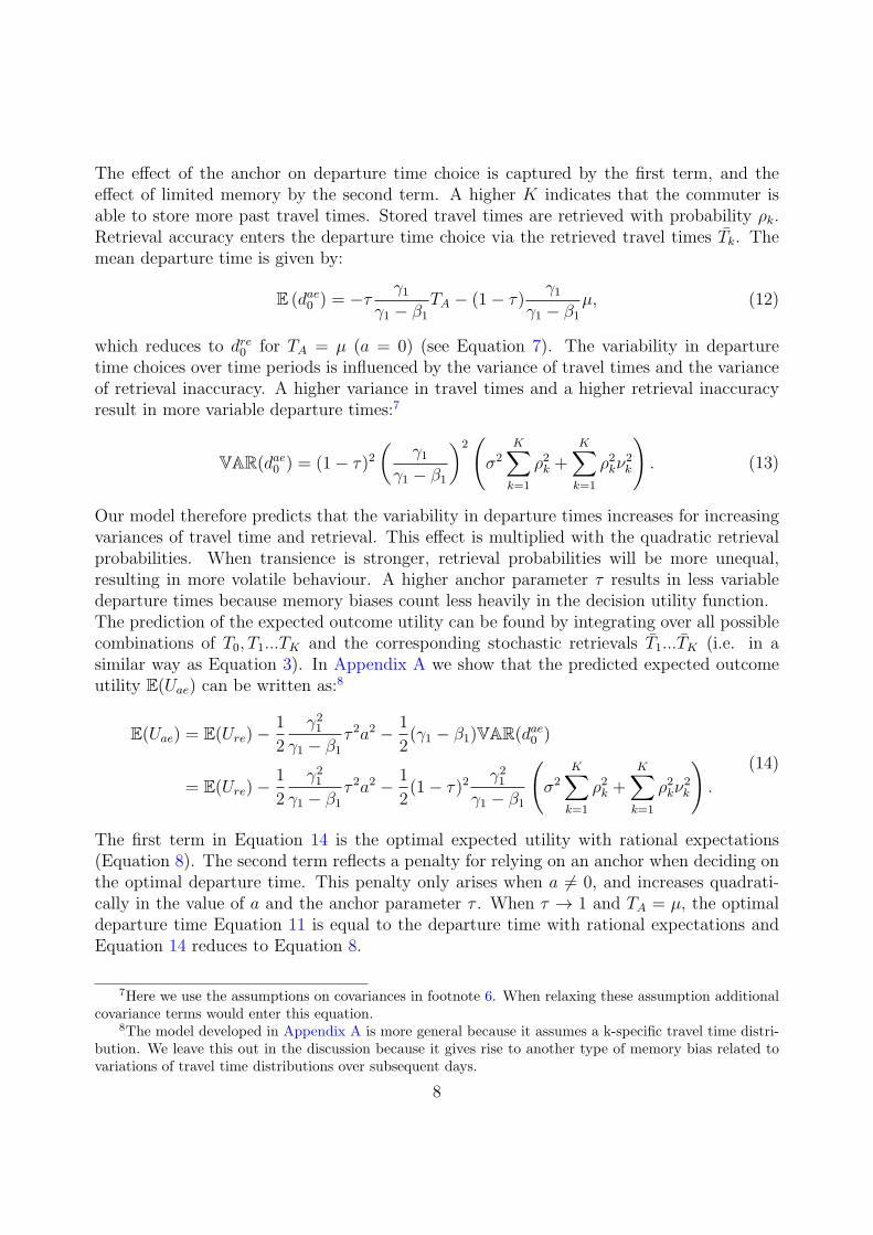
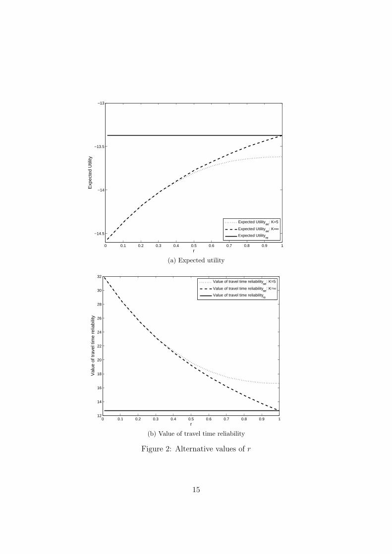
The first deviation introduced from the rational expectations outcome is transience. Indi-viduals are assumed to store only K past travel time experiences, where K is set to eitherK = 5 or K = 100. We systematically change the importance of each of these past expe-riences in forming expectations by changing the transience parameter r (see Equation 16).Increasing values of r result in a more equal distribution of weights attached across all mem-ories, whereas smaller values assign more weight to more recent periods. We vary r betweenits upper bound of r = 1 (equal weights for all K experienced travel times) and r = 0.5at which the most recent period receives a weight of approximately 50% (i.e. ρ1 ≈ 0.5) forboth levels of K. Moreover, we assume that the past realisations of Tk are all accuratelyretrieved, such that Tk = Tk and ν2

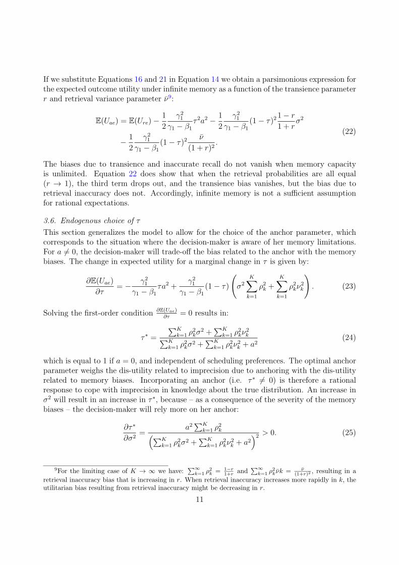
k = 0 , ∀k. And for the moment, we ignore anchoring bysetting τ = 0. We generate 1,000 different sets of K travel time realisations and depict theoptimal departure times in Figure 1. A comparison between Figures 1a and 1b highlightsthat limited storage capacity (K = 5 instead of K = 100) increases the variance of theoptimal departure time considerably. This is a direct consequence of adaptive expectationsbeing formed by a smaller number of travel time realisations. Figures 1c and 1d illustratethat for smaller values of r, the size of K becomes less relevant for the variance of optimaldeparture times. By definition, reducing r shifts attention towards more recent periods suchthat more distant travel time realisations have a negligible impact on the optimal departuretime.Transience has direct implications on the level of expected outcome utility as illustrated byFigure 2a. Even when r → 1, expected outcome utility falls below EUre forK < ∞, becausecommuters have limited memory capacity to form rational expectations. A decrease in rresults in a further deviation of EUae from EUre because more weight is given to more recentperiods. A similar insight is found for the VOR in Figure 2b. Limited memory increases thevalue of reliability and the penalty is amplified for higher degrees of transience. Equations 9and 18 indeed confirm that the distance between V ORre and V ORae decreases for increasingK. The maximum distance between these two lines is in our case 1

2γ12

(γ1−β1)= AC19.51 per hour

for K = 1. The latter results in a maximum VOR of AC32.22 per hour, which is about 2.5times higher than the rational expectations outcome. Cantarella (2013) suggests values of40-80% for the weight of the most recent experience in the expectation of the current trafficsituations. When we assume r = 0.5 and K = 5, the most recent travel time experiencedetermines about 50% of the travel time expectation and the value of travel time reliabilityis AC19.63, which is 45% higher than with rational expectations.

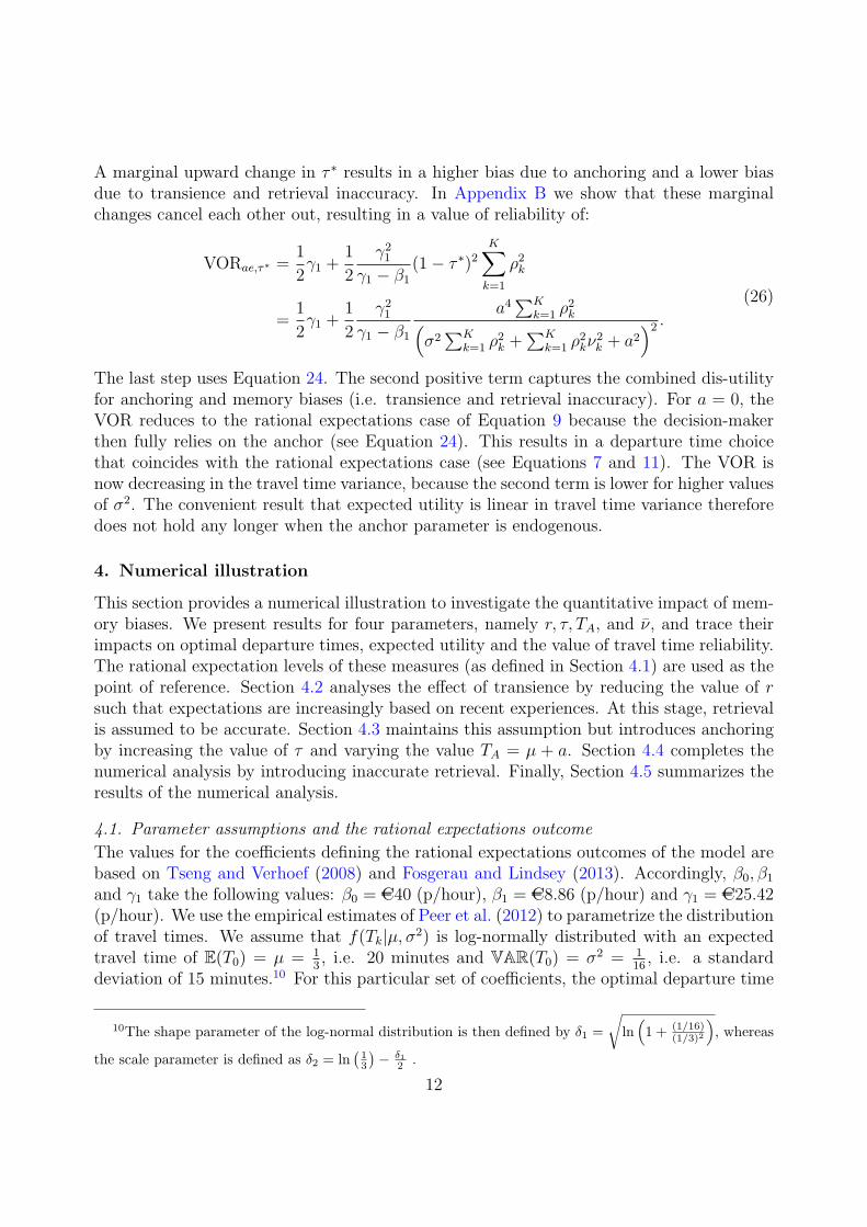
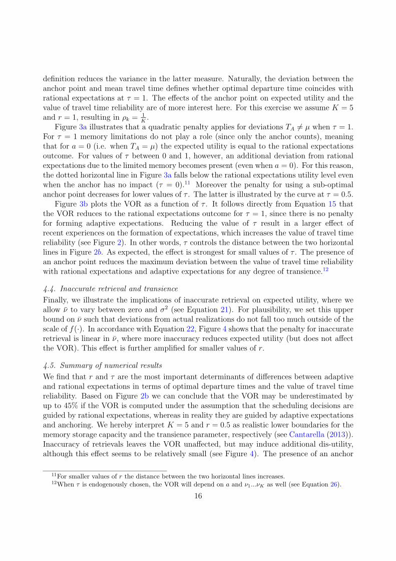
4.3. Accurate retrieval and anchored expectations

So far we have neglected the presence of an anchor. Equation 11 shows that commutersdepart earlier when they have a higher anchor value TA. Moreover, an increase in τ reducesthe influence of past travel time realizations on the optimal departure time and therefore by

13

0 100 200 300 400 500 600 700 800 900 1000−2

−1.8

−1.6

−1.4

−1.2

−1

−0.8

−0.6

−0.4

−0.2

0

1,000 different sets of travel time realisations

Opt

imal

dep

artu

re ti

me

doae

dore

(a) K=5, r=1

0 100 200 300 400 500 600 700 800 900 1000−2

−1.8

−1.6

−1.4

−1.2

−1

−0.8

−0.6

−0.4

−0.2

0

1,000 different sets of travel time realisations

Opt

imal

dep

artu

re ti

me

doae

dore

(b) K=100, r=1

0 100 200 300 400 500 600 700 800 900 1000−2

−1.8

−1.6

−1.4

−1.2

−1

−0.8

−0.6

−0.4

−0.2

0

1,000 different sets of travel time realisations

Opt

imal

dep

artu

re ti

me

doae

dore

(c) K=5, r=0.5

0 100 200 300 400 500 600 700 800 900 1000−2

−1.8

−1.6

−1.4

−1.2

−1

−0.8

−0.6

−0.4

−0.2

0

1,000 different sets of travel time realisations

Opt

imal

dep

artu

re ti

me

doae

dore

(d) K=100, r=0.5

Figure 1: Variations in optimal departure time given K and r

14

0 0.1 0.2 0.3 0.4 0.5 0.6 0.7 0.8 0.9 1

−14.5

−14

−13.5

−13

r

Exp

ecte

d U

tility

Expected Utilityae

: K=5

Expected Utilityae

: K=∞

Expected Utilityre

(a) Expected utility

0 0.1 0.2 0.3 0.4 0.5 0.6 0.7 0.8 0.9 112

14

16

18

20

22

24

26

28

30

32

r

Val

ue o

f tra

vel t

ime

relia

bilit

y

Value of travel time reliability

ae: K=5

Value of travel time reliabilityae

: K=∞

Value of travel time reliabilityre

(b) Value of travel time reliability

Figure 2: Alternative values of r

15

definition reduces the variance in the latter measure. Naturally, the deviation between theanchor point and mean travel time defines whether optimal departure time coincides withrational expectations at τ = 1. The effects of the anchor point on expected utility and thevalue of travel time reliability are of more interest here. For this exercise we assume K = 5and r = 1, resulting in ρk =

1K.

Figure 3a illustrates that a quadratic penalty applies for deviations TA 6= µ when τ = 1.For τ = 1 memory limitations do not play a role (since only the anchor counts), meaningthat for a = 0 (i.e. when TA = µ) the expected utility is equal to the rational expectationsoutcome. For values of τ between 0 and 1, however, an additional deviation from rationalexpectations due to the limited memory becomes present (even when a = 0). For this reason,the dotted horizontal line in Figure 3a falls below the rational expectations utility level evenwhen the anchor has no impact (τ = 0).11 Moreover the penalty for using a sub-optimalanchor point decreases for lower values of τ . The latter is illustrated by the curve at τ = 0.5.

Figure 3b plots the VOR as a function of τ . It follows directly from Equation 15 thatthe VOR reduces to the rational expectations outcome for τ = 1, since there is no penaltyfor forming adaptive expectations. Reducing the value of τ result in a larger effect ofrecent experiences on the formation of expectations, which increases the value of travel timereliability (see Figure 2). In other words, τ controls the distance between the two horizontallines in Figure 2b. As expected, the effect is strongest for small values of τ . The presence ofan anchor point reduces the maximum deviation between the value of travel time reliabilitywith rational expectations and adaptive expectations for any degree of transience.12

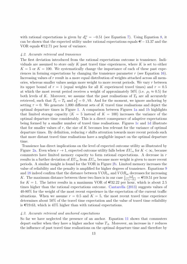
4.4. Inaccurate retrieval and transience

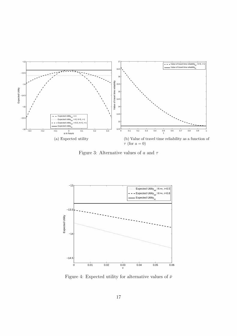
Finally, we illustrate the implications of inaccurate retrieval on expected utility, where weallow ν to vary between zero and σ2 (see Equation 21). For plausibility, we set this upperbound on ν such that deviations from actual realizations do not fall too much outside of thescale of f(·). In accordance with Equation 22, Figure 4 shows that the penalty for inaccurateretrieval is linear in ν, where more inaccuracy reduces expected utility (but does not affectthe VOR). This effect is further amplified for smaller values of r.

4.5. Summary of numerical results

We find that r and τ are the most important determinants of differences between adaptiveand rational expectations in terms of optimal departure times and the value of travel timereliability. Based on Figure 2b we can conclude that the VOR may be underestimated byup to 45% if the VOR is computed under the assumption that the scheduling decisions areguided by rational expectations, whereas in reality they are guided by adaptive expectationsand anchoring. We hereby interpret K = 5 and r = 0.5 as realistic lower boundaries for thememory storage capacity and the transience parameter, respectively (see Cantarella (2013)).Inaccuracy of retrievals leaves the VOR unaffected, but may induce additional dis-utility,although this effect seems to be relatively small (see Figure 4). The presence of an anchor

11For smaller values of r the distance between the two horizontal lines increases.12When τ is endogenously chosen, the VOR will depend on a and ν1...νK as well (see Equation 26).

16

−0.3 −0.2 −0.1 0 0.1 0.2 0.3−16

−15.5

−15

−14.5

−14

−13.5

−13

a in hours

Exp

ecte

d U

tility

Expected Utilityae

: τ=1

Expected Utilityae

: τ=0, K=5, r=1

Expected Utilityae

: τ=0.5, K=5, r=1

Expected Utilityre

(a) Expected utility

0 0.1 0.2 0.3 0.4 0.5 0.6 0.7 0.8 0.9 112.5

13

13.5

14

14.5

15

15.5

16

16.5

17

τ

Val

ue o

f tra

vel t

ime

relia

bilit

y

Value of travel time reliability

ae: K=5, r=1

Value of travel time reliabilityre

(b) Value of travel time reliability as a function ofτ (for a = 0)

Figure 3: Alternative values of a and τ

0 0.01 0.02 0.03 0.04 0.05 0.06

−14.5

−14

−13.5

−13

ν

Exp

ecte

d U

tility

Expected Utilityae

: K=∞, r=0.5

Expected Utilityae

: K=∞, r=0.8

Expected Utilityre

Figure 4: Expected utility for alternative values of ν

17

(τ 6= 0) may under certain conditions increase the expected utility. When τ is exogenous,an increase in τ always decreases the bias in the VOR, which is in turn independent of theanchor itself.

5. Conclusions

We developed a model in which adaptive expectations are formed on the basis of past experi-ences and anchoring. Limited memory storage capacity, transience, inaccurate retrieval andanchoring result in sub-optimal decisions, and thereby translate into reductions in utilityrelative to the rational expectations outcome. We apply our model to scheduling choices ofcommuters during the morning commute, where travel times are stochastic. We show thatthe value of travel time reliability may be underestimated by up to 45% if rational expec-tations are assumed, while the true expectation formation process is adaptive. The benefitsfrom reliability improvements thus tend to be significantly larger if travel time expectationformation is guided by limited memory, adaptive expectations and anchoring. Revealed pref-erence studies that use a reduced-form utility function probably already capture the biasesformulated in this paper. Our results are therefore mainly important for stated preferenceanalyses that ignore the process of expectation formation.

Our functional form assumptions on the utility function allowed us to derive a simpleclosed-form expression for the memory adjusted value of reliability. The analytical result hasthe potential to be incorporated in existing static transport network models. Equations 8and 14 show that trip travel cost functions of the structure C = b1 + b2µ + b3µ

2 + b4σ2 are

able to capture memory biases in an adequate way. Here, the parameters b1, b2, b3 and b4 arefunctions of the underlying behavioural parameters related to scheduling (β0, β1 and γ1),anchoring (τ and a), transience (ρ1, ..., ρK) and retrieval inaccuracy (ν1, ..., νK), and µ andσ2 are functions of the number of travellers on the links that constitute the trip. For moregeneral forms of the utility function this structure unfortunately breaks down and numericalanalysis is needed.

Our dynamic memory model stands apart from static behavioural models where individ-uals treat probabilities in a non-rational way, since it predicts that commuters are sometimesoptimistic and sometimes pessimistic, depending on their most recent experiences and cor-responding retrieval probabilities. This is in contrast to rank-dependent utility models thatassume that optimism and pessimism are exogenously given and therefore unrelated to ear-lier experiences (see Koster and Verhoef (2012) and Xiao and Fukuda (2015) for transportapplications).

Our approach may serve as an input for the modelling of dynamic systems, both intransport as well as in other fields of economics. In such models adaptive expectations oftenplay a central role but are usually based on simple decision rules (see for example Watlingand Cantarella (2013) for an overview of day-to-day dynamic transport systems and Hommes(2013) for an overview of adaptive expectations in financial markets). Incorporating dynamiclearning mechanisms in the model is a fruitful area for further investigation.

Although our model is fairly general, we made several restrictive assumptions in order tokeep it analytically tractable. Some of the assumptions can be adjusted in order to arrive at

18

more general results. In the next paragraphs, several possible generalizations are discussed.First, we assume for simplicity that travel time distributions are independent of departure

time, whereas in reality travel time distributions usually vary by time of day. In AppendixA we show how to generalize the resulting expressions for travel time distributions that arechanging over subsequent days. This results in additional biases related to variations intravel time distributions over subsequent time periods.

Second, we assume that the decision-maker has a fixed anchor TA = µ + a, whereasin reality this may well be a noisy belief, implying that a is random. The implicationsof randomness in the anchor can be discussed by looking at the impact on the varianceand the mean departure time with adaptive expectations. Equation 12 then will includethe mean anchor, whereas Equation 13 would have an additional variance term relating tothe variation in the anchor. Because the variance of departure time will increase with ahigher variance in the anchor, this will result in additional losses in expected utility (seeEquation A.3).

Third, for the main analysis (except for Section 3.6, where we discuss the endogenouschoice of the relative weight attached to the anchor, τ), we made the assumption thatdecision makers are not aware of their memory limitations (Piccione and Rubinstein, 1997).For decisions where the stakes are not so high, this may be a reasonable assumption. Whenthe utilitarian effects of sub-optimal choice are high, the decision maker may take a morereflective attitude and may optimise her anchor or collect additional information in order toreduce behavioural biases.

Fourth, we assumed that retrieval probabilities are independent of the values of theexperienced states, meaning that negative experiences do not impact expectations morethan positive ones, or vice versa. Furthermore, we assumed that the experience of a newstate does not affect the memory of the already stored states. Future research should aimat relaxing these assumptions.

Further useful generalizations could be implemented with respect to the specificationof the scheduling preferences as well as by including information. One might for instanceemploy more general scheduling preferences and then use Taylor approximations to arriveat more general results (see Engelson (2011)). It also seems a fruitful direction for futureresearch to extend the model by the possibility to obtain information about future traveltimes. The quality of the information could then in turn depend on when the informationis collected, or on how much one is willing to pay for it.

Finally, we consider the empirical testing of our decision model using laboratory andrevealed preference data as a fruitful direction for further research. However, the datarequirements will be demanding: high-quality panel data with a substantial sample size willbe necessary to estimate the parameters of our model in such a way that the four maincomponents of the model (limited memory capacity, transience, retrieval accuracy and theanchor) can be unambiguously disentangled. For initial applications, it may therefore beuseful to disregard one of the components, or to make functional form assumptions thatreduce the number of parameters to be estimated.

19

Bibliography

Arentze, T. A. and Timmermans, H. J. (2003). Modeling learning and adaptation processes in activity-travelchoice a framework and numerical experiment. Transportation, 30(1):37–62.

Arentze, T. A. and Timmermans, H. J. (2005). Representing mental maps and cognitive learning in micro-simulation models of activity-travel choice dynamics. Transportation, 32(4):321–340.

Ariely, D., Loewenstein, G., and Prelec, D. (2003). ”Coherent arbitrariness”: Stable demand curves withoutstable preferences. The Quarterly Journal of Economics, 118(1):73–106.

Avineri, E. and Prashker, J. N. (2005). Sensitivity to travel time variability: Travelers learning perspective.Transportation Research Part C: Emerging Technologies, 13(2):157–183.

Barucci, E. (1999). Heterogeneous beliefs and learning in forward looking economic models. Journal of

Evolutionary Economics, 9(4):453–464.Barucci, E. (2000). Exponentially fading memory learning in forward-looking economic models. Journal of

Economic Dynamics and Control, 24(5):1027–1046.Ben-Elia, E. and Shiftan, Y. (2010). Which road do I take? a learning-based model of route-choice behavior

with real-time information. Transportation Research Part A: Policy and Practice, 44(4):249 – 264.Benabou, R. and Tirole, J. (2002). Self-confidence and personal motivation. The Quarterly Journal of

Economics, 117(3):871–915.Bernheim, D. B. and Thomadsen, R. (2005). Memory and anticipation. The Economic Journal,

115(503):271–304.Bogers, E. A. I., Bierlaire, M., and Hoogendoorn, S. P. (2007). Modeling learning in route choice. Trans-

portation Research Record, 2014:1–8.Borjesson, M., Eliasson, J., and Franklin, J. P. (2012). Valuations of travel time variability in scheduling

versus mean–variance models. Transportation Research Part B: Methodological, 46(7):855 – 873.Brunnermeier, M. K. and Parker, J. A. (2005). Optimal expectations. American Economic Review,

4(95):1092 – 1118.Cantarella, G. E. (2013). Day-to-day dynamic models for intelligent transportation systems design and

appraisal. Transportation Research Part C: Emerging Technologies, 29:117–130.Caplin, A., Dean, M., and Martin, D. (2011). Search and satisficing. American Economic Review,

101(7):2899–2922.Chen, R. and Mahmassani, H. (2004). Travel time perception and learning mechanisms in traffic networks.

Transportation Research Record, 1894(1):209–221.Engelson, L. (2011). Properties of Expected Cost Function with Uncertain Travel Time. Transportation

Research Record, 2254:151–159.Fosgerau, M. and Engelson, L. (2011). The value of travel time variance. Transportation Research Part B:

Methodological, 45(1):1–8.Fosgerau, M. and Karlstrom, A. (2010). The value of reliability. Transportation Research Part B: Method-

ological, 44:38–49.Fosgerau, M. and Lindsey, R. (2013). Trip-timing decisions with traffic incidents. Regional Science and

Urban Economics, 43(5):764–782.Furnham, A. and Boo, H. C. (2011). A literature review of the anchoring effect. The Journal of Socio-

Economics, 40(1):35 – 42.Gennaioli, N. and Shleifer, A. (2010). What comes to mind. The Quarterly Journal of Economics,

125(4):1399–1433.Gollier, C. and Muermann, A. (2010). Optimal choice and beliefs with ex ante savoring and ex post

disappointment. Management Science, 56(8):1272–1284.Hensher, D. (2001). The valuation of commuter travel time savings for car drivers: evaluating alternative

model specifications. Transportation, 28(2):101–118.Hirshleifer, D. and Welch, I. (2002). An economic approach to the psychology of change: Amnesia, inertia,

and impulsiveness. Journal of Economics & Management Strategy, 11(3):379–421.Hommes, C. (2013). Behavioral rationality and heterogeneous expectations in complex economic systems.

Cambridge University Press.

20

Horowitz, J. L. (1984). The stability of stochastic equilibrium in a two-link transportation network. Trans-portation Research Part B: Methodological, 18(1):13–28.

Jha, M., Madanat, S., and Peeta, S. (1998). Perception updating and day-to-day travel choice dynamicsin traffic networks with information provision. Transportation Research Part C: Emerging Technologies,6(3):189–212.

Koster, P. and Verhoef, E. T. (2012). A rank-dependent scheduling model. Journal of Transport Economics

and Policy, 46(1):123–138.Mullainathan, S. (2002). A memory-based model of bounded rationality. The Quarterly Journal of Eco-

nomics, 117(3):735–774.Noland, R. B. and Small, K. A. (1995). Travel-time Uncertainty, Departure Time Choice, and the Cost of

Morning Commutes. Transportation Research Record, 1493:150–158.Peer, S., Koopmans, C. C., and Verhoef, E. T. (2012). Prediction of travel time variability for cost-benefit

analysis. Transportation Research Part A: Policy and Practice, 46(1):79–90.Peer, S., Verhoef, E. T., Knockaert, J., Koster, P., and Tseng, Y.-Y. (2015). Long-run vs. short-run

perspectives on consumer scheduling: Evidence from a revealed-preference experiment among peak-hourroad commuters. International Economic Review, 56(1):303–323.

Piccione, M. and Rubinstein, A. (1997). On the interpretation of decision problems with imperfect recall.Games and Economic Behavior, 20(1):3 – 24.

Sarafidis, Y. (2007). What Have you Done for me Lately? Release of Information and Strategic Manipulationof Memories. The Economic Journal, 117(518):307–326.

Schacter, D. L. (2002). The seven sins of memory: How the mind forgets and remembers. Houghton-Mifflin,New York.

Simon, H. A. (1955). A behavioral model of rational choice. The Quarterly Journal of Economics, 69(1):99–118.

Small, K. A. (1982). The Scheduling of Consumer Activities : Work Trips. The American Economic Review,72:467–479.

Small, K. A. (1992). Trip scheduling in urban transportation analysis. The American Economic Review,82(2):482–486.

Strack, F. and Mussweiler, T. (1997). Explaining the enigmatic anchoring effect: Mechanisms of selectiveaccessibility. Journal of Personality and Social Psychology, 73(3):437.

Tseng, Y.-Y. and Verhoef, E. T. (2008). Value of time by time of day: A stated-preference study. Trans-

portation Research Part B: Methodological, 42(7-8):607–618.Tversky, A. and Kahneman, D. (1974). Judgment under uncertainty: Heuristics and biases. Science,

185(4157):1124–1131.Vickrey, W. S. (1969). Congestion theory and transport investment. American Economic Review, 59(2):251–

260.Vickrey, W. S. (1973). Pricing, metering, and efficiently using urban transportation facilities. Highway

Research Record, 476:36–48.Watling, D. P. and Cantarella, G. E. (2013). Modelling sources of variation in transportation systems:

theoretical foundations of day-to-day dynamic models. Transportmetrica B: Transport Dynamics, 1(1):3–32.

Wilson, A. (2003). Bounded memory and biases in information processing. Econometrica, 6(82):2257–2294.Wilson, T. D., Houston, C. E., Etling, K. M., and Brekke, N. (1996). A new look at anchoring effects: basic

anchoring and its antecedents. Journal of Experimental Psychology: General, 125(4):387–402.Xiao, Y. and Fukuda, D. (2015). On the cost of misperceived travel time variability. Transportation Research

Part A, (75):96–112.

21

Appendix A. Proof section 3.3.

In this Appendix we derive the predicted expected outcome utility (Equation 14). The proofis for general travel distributions with k-dependent means and variances and k-dependentanchoring. Assume that travel time distributions have mean µk and variance σ2

k and prob-ability density f(Tk|µk, σ

2k). The predicted expected outcome utility is given by:

E(Uae) ≡ E (U(dae0 , T0))

=

∫

...

∫

(

∫

...

∫

U(dae0 , T0)K∏

k=1

g(

Tk|Tk, ν2k

)

dT1...TK)

)

K∏

k=0

f(Tk|µk, σ2k)dT0...dTK ,

(A.1)

The expectation over all values of T0 is given by:

ET0(U(dae0 , T0)) =

∫

(

−

∫ 0

dae0

(β0 + β1v)dv −

∫ dae0

+T0

0

(β0 + γ1v)dv

)

f(T0|µ0, σ20)dT0

= −β0µ0 −1

2(γ1 − β1)(d

ae0 )2 − γ1µ0d

ae0 −

1

2γ1(µ

20 + σ2

0),

(A.2)

where we use ET0to emphasize that the expectation is only over values of T0. The predicted

expected outcome utility with adaptive expectation can be found by taking the expectedvalue over all possible values of the departure time dae0 :

E(Uae) = E

(

−β0µ0 −1

2(γ1 − β1)(d

ae0 )2 − γ1µ0d

ae0 −

1

2γ1(µ

20 + σ2

0)

)

= −β0µ0 −1

2(γ1 − β1)E

(

(dae0 )2)

− γ1µ0E(dae0 )−

1

2γ1(µ

20 + σ2

0)

= −β0µ0 −1

2(γ1 − β1)

(

(E(dae0 ))2 + VAR(dae0 ))

− γ1µ0E(dae0 )−

1

2γ1(µ

20 + σ2

0).

(A.3)

This shows that E(Uae) can be written as a function of the mean departure time and thevariance of departure time. When travel time distributions depend on k, the departure timewith adaptive expectations is given by 11. The mean departure time is given by:

E (dae0 ) = −τγ1

γ1 − β1

TA − (1− τ)γ1

γ1 − β1

K∑

k=1

ρkµk, (A.4)

which reduces to 12 for µk = µ. The variance of the departure time is given by (here we usethe assumptions of footnote 6):

VAR(dae0 ) = (1− τ)2(

γ1γ1 − β1

)2 K∑

k=1

ρ2k(

σ2k + ν2

k

)

, (A.5)

which reduces to 13, for σ2k = σ2. Substituting Equation A.4 and A.5 in Equation A.3 gives

the result for k-dependent travel time distributions. For the remainder of this Appendix we

22

assume µk = µ0 = µ and σ2k = σ2

0 = σ2 in order to arrive at the results that are discussed inthe main body of the paper. Substituting 12 in A.3 gives:

E(Uae) = −β0µ−1

2(γ1 − β1)

(

(

γ1γ1 − β1

)2(

µ2 + 2µτa+ τ 2a2)

+ VAR(dae0 )

)

+γ21

γ1 − β1

(

µ2 + µτa)

−1

2γ1(µ

2 + σ2)

= −β0µ+1

2

γ21

γ1 − β1

−1

2γ1µ

2 −1

2γ1σ

2 −1

2

γ21

γ1 − β1

τ 2a2 −1

2(γ1 − β1)VAR(d

ae0 )

= −β0µ+1

2

β1γ1γ1 − β1

µ2 −1

2γ1σ

2 −1

2

γ21

γ1 − β1

τ 2a2 −1

2(γ1 − β1)VAR(d

ae0 )

= E(Ure)−1

2

γ21

γ1 − β1

τ 2a2 −1

2(γ1 − β1)VAR(d

ae0 ).

(A.6)

Substituting Equation 13 gives the desired result. This concludes the proof.

Appendix B. Proof section 3.6.

We start with 14 where we include the optimal anchor parameter τ ∗ which depends on thevariance of travel time (see 24). Then differentiate expected utility with respect to σ2 toobtain:

VORτ∗ =1

2γ1 +

1

2

γ21

γ1 − β1

(1− τ ∗)2K∑

k=1

ρ2k +γ21

γ1 − β1

τ ∗∂τ ∗

∂σ2a2

−γ21

γ1 − β1

(1− τ ∗)∂τ ∗

∂σ2

(

σ2

K∑

k=1

ρ2k +K∑

k=1

ρ2kν2k

)

=1

2γ1 +

1

2

γ21

γ1 − β1

(1− τ ∗)2K∑

k=1

ρ2k

+γ21

γ1 − β1

(

τ ∗∂τ ∗

∂σ2a2 − (1− τ ∗)

∂τ ∗

∂σ2

(

σ2

K∑

k=1

ρ2k +K∑

k=1

ρ2kν2k

))

=1

2γ1 +

1

2

γ21

γ1 − β1

(1− τ ∗)2K∑

k=1

ρ2k

+γ21

γ1 − β1

∂τ ∗

∂σ2

(

τ ∗

(

a2 + σ2

K∑

k=1

ρ2k +K∑

k=1

ρ2kν2k

)

−

(

σ2

K∑

k=1

ρ2k +K∑

k=1

ρ2kν2k

))

=1

2γ1 +

1

2

γ21

γ1 − β1

(1− τ ∗)2K∑

k=1

ρ2k,

(B.1)

23

Substituting 24 gives:

VORτ∗ =1

2γ1 +

1

2

γ21

γ1 − β1

(

a2

σ2∑K

k=1 ρ2k +

∑K

k=1 ρ2kν

2k + a2

)2 K∑

k=1

ρ2k

=1

2γ1 +

1

2

γ21

γ1 − β1

a4∑K

k=1 ρ2k

(

σ2∑K

k=1 ρ2k +

∑K

k=1 ρ2kν

2k + a2

)2 ,

(B.2)

24