MEM 255: Introduction to MATLAB Professor Kwatny

Contents MEM 255: Introduction to MATLAB ........................................................................................................ 1

Contents......................................................................................................................................................... 1

Basics ............................................................................................................................................................. 2 Command Window ..................................................................................................................................... 2 m-files – scripts and functions.................................................................................................................... 2 Basic Data Structures – vectors, matrices and polynomials ...................................................................... 3

Vectors................................................................................................................................................... 3 Matrices ................................................................................................................................................. 4 Example:................................................................................................................................................ 5 Polynomials ........................................................................................................................................... 5

Basic Plotting ................................................................................................................................................ 6 Simple Line Plots ....................................................................................................................................... 6

Frequency Domain Modeling ...................................................................................................................... 7 Complex Numbers ...................................................................................................................................... 7 Transfer Functions..................................................................................................................................... 8

Creating Transfer Functions .................................................................................................................. 8 Converting between Forms.................................................................................................................... 8 Laplace Transforms ............................................................................................................................... 9

Analysis Tools ............................................................................................................................................ 9 Root Locus............................................................................................................................................. 9 Bode..................................................................................................................................................... 10 Nyquist ................................................................................................................................................ 10 SISO Tool & LTI Viewer .................................................................................................................... 11

State Space Models ..................................................................................................................................... 13 Converting between State Space and Transfer Function Objects ............................................................ 14

Computing Step Responses........................................................................................................................ 15

Interconnections ......................................................................................................................................... 16

Eigenvalues & Eigenvectors ...................................................................................................................... 17 Chain of Three Inertias ............................................................................................................................ 17 Antenna Positioning System..................................................................................................................... 19

Solving Ordinary Differential Equations ................................................................................................. 20

MEM 255 MATLAB Notes Professor Kwatny

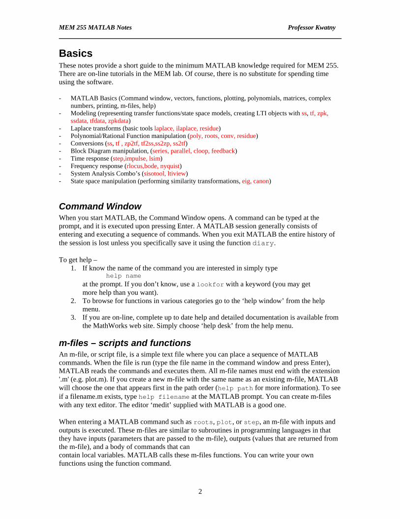
Basics These notes provide a short guide to the minimum MATLAB knowledge required for MEM 255. There are on-line tutorials in the MEM lab. Of course, there is no substitute for spending time using the software. - MATLAB Basics (Command window, vectors, functions, plotting, polynomials, matrices, complex

numbers, printing, m-files, help) - Modeling (representing transfer functions/state space models, creating LTI objects with ss, tf, zpk,

ssdata, tfdata, zpkdata) - Laplace transforms (basic tools laplace, ilaplace, residue) - Polynomial/Rational Function manipulation (poly, roots, conv, residue) - Conversions (ss, tf , zp2tf, tf2ss,ss2zp, ss2tf) - Block Diagram manipulation, (series, parallel, cloop, feedback) - Time response (step,impulse, lsim) - Frequency response (rlocus,bode, nyquist) - System Analysis Combo’s (sisotool, ltiview) - State space manipulation (performing similarity transformations, eig, canon)

Command Window When you start MATLAB, the Command Window opens. A command can be typed at the prompt, and it is executed upon pressing Enter. A MATLAB session generally consists of entering and executing a sequence of commands. When you exit MATLAB the entire history of the session is lost unless you specifically save it using the function diary. To get help –

1. If know the name of the command you are interested in simply type help name

at the prompt. If you don’t know, use a lookfor with a keyword (you may get more help than you want).

2. To browse for functions in various categories go to the ‘help window’ from the help menu.

3. If you are on-line, complete up to date help and detailed documentation is available from the MathWorks web site. Simply choose ‘help desk’ from the help menu.

m-files – scripts and functions An m-file, or script file, is a simple text file where you can place a sequence of MATLAB commands. When the file is run (type the file name in the command window and press Enter), MATLAB reads the commands and executes them. All m-file names must end with the extension '.m' (e.g. plot.m). If you create a new m-file with the same name as an existing m-file, MATLAB will choose the one that appears first in the path order (help path for more information). To see if a filename.m exists, type help filename at the MATLAB prompt. You can create m-files with any text editor. The editor ‘medit’ supplied with MATLAB is a good one. When entering a MATLAB command such as roots, plot, or step, an m-file with inputs and outputs is executed. These m-files are similar to subroutines in programming languages in that they have inputs (parameters that are passed to the m-file), outputs (values that are returned from the m-file), and a body of commands that can contain local variables. MATLAB calls these m-files functions. You can write your own functions using the function command.

2

MEM 255 MATLAB Notes Professor Kwatny

The new function must be given a filename with a '.m' extension. This file should be saved in any directory that is in MATLAB's search path. The first line of the file must be in the form: function [output1,output2] = filename(input1,input2,input3) A function can have any number of input and output variables.

Basic Data Structures – vectors, matrices and polynomials

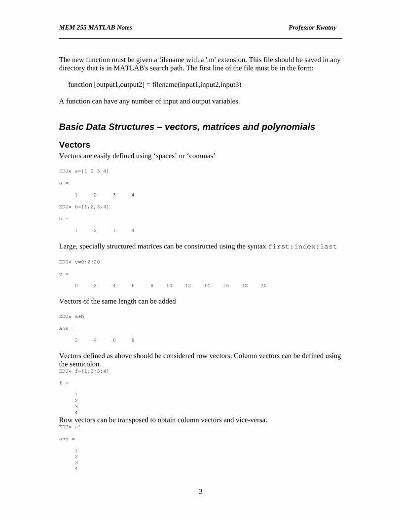
Vectors Vectors are easily defined using ‘spaces’ or ‘commas’ EDU» a=[1 2 3 4] a = 1 2 3 4 EDU» b=[1,2,3,4] b = 1 2 3 4

Large, specially structured matrices can be constructed using the syntax first:index:last EDU» c=0:2:20 c = 0 2 4 6 8 10 12 14 16 18 20

Vectors of the same length can be added EDU» a+b ans = 2 4 6 8

Vectors defined as above should be considered row vectors. Column vectors can be defined using the semicolon. EDU» f=[1;2;3;4] f = 1 2 3 4

Row vectors can be transposed to obtain column vectors and vice-versa. EDU» a' ans = 1 2 3 4

3

MEM 255 MATLAB Notes Professor Kwatny

Matrices Matrices can be defined in a similar way to vectors, with rows separated by semicolons. EDU» A=[1 2 3;4 5 6;7 8 9] A = 1 2 3 4 5 6 7 8 9 EDU» B=[0,1,0;0,0,1] B = 0 1 0 0 0 1

Matrices of compatible dimensions can be multiplied EDU» B*A ans = 4 5 6 7 8 9

They can b raised to powers EDU» A^3 ans = 468 576 684 1062 1305 1548 1656 2034 2412

Element by element multiplication of square matrices is accomplished by the .* or .^ operator. For example EDU» A.^3 ans = 1 8 27 64 125 216 343 512 729 cubes each element of A. Matrices can be transposed EDU» B' ans = 0 0 1 0 0 1

Table 1. Functions to create matrices Function Returns diag matrix with specified diagonal elements/or extracts diagonal entries eye identity matrix ones matrix filled with ones rand matrix filled with random numbers zeros matrix filled with zeros linspace row vector of linear spaced elements

4

MEM 255 MATLAB Notes Professor Kwatny

logspace row vector of logarithmically spaced elements

Example: >> eye(4) ans = 1 0 0 0 0 1 0 0 0 0 1 0 0 0 0 1

Polynomials A polynomials can be represented by a vector containing its oredered coefficient list. The polynomial 4 3 22 4s s s s 3+ + + + is defined EDU» poly1=[1 2 4 1 3] poly1 = 1 2 4 1 3 and the polynomial 2 1s + is defined EDU» poly2=[1 0 1] poly2 = 1 0 1

Certain MATLAB functions interpret 1n + dimensional vectors as -th order polynomials. These include polyval, roots, conv and deconv. Polyval can be used to evaluate polynomials, roots determines the roots of the given polynomial, conv multiplies two polynomials, and deconv divides two polynomials.

n

EDU» conv(poly1,poly2) ans = 1 2 5 3 7 1 3 EDU» [x,R]=deconv(poly1,poly2) x = 1 2 3 R = 0 0 0 -1 0

Notice that this last result states

4 3 2

22 2

2 4 3 2 31 1

s s s s ss ss s

+ + + + −= + + +

+ +

The characteristic polynomial of a square matrix can be obtained EDU» x=poly(A) x =

5

MEM 255 MATLAB Notes Professor Kwatny

1.0000 -15.0000 -18.0000 -0.0000

Allowing us to compute the eigenvalues of the matrix EDU» roots(x) ans = 16.1168 -1.1168 -0.0000

Basic Plotting

Simple Line Plots The basic form is define data vectors x and y then plot(x,y). >> xdata=[0,1,2,3,4,5];ydata=[1,2,3,3,2,1]; >> plot(xdata,ydata)

You can also create subplots: >> x=linspace(0,2*pi); >> subplot(1,2,1); >> plot(x,sin(x)); axis([0 2*pi -1.5 1.5]); title('sin(x)'); >> subplot(1,2,2); >> plot(x,sin(2*x)); axis([0 2*pi -1.5 1.5]); title('sin(2x)');

6

MEM 255 MATLAB Notes Professor Kwatny

Frequency Domain Modeling

Complex Numbers Note that in MALAB, both i and j are predefined as 1− . For instance compute >> j^2 ans = -1 >> i^(3/2) ans = -0.7071 + 0.7071i

However, you can redefine them as something else. Once you do, the original definitions are gone. >> j=5; j^2 ans = 25

A complex number is ordinarily expressed in rectangular coordinates z x iy= + where x is the ‘real’ part and y is the ‘imaginary’ part, or, alternatively, in polar or Euler notation iz e θρ= , where ρ is the ‘magnitude’ and θ is the ‘angle.’ Table 2. Operations on complex numbers Function Returns imag imaginary part of a complex number real real part of a complex number abs magnitude of a complex number angle angle of a complex number conj conjugate of a complex number Example: >> z=1+i

7

MEM 255 MATLAB Notes Professor Kwatny

z = 1.0000 + 1.0000i >> abs(z) ans = 1.4142 >> angle(z)*180/pi ans = 45

Transfer Functions

Creating Transfer Functions 1. numerical using the functions tf or zpk 2. symbolic

EDU» numf=10*[1 2]; EDU» denf=[1 6 9]; EDU» F=tf(numf,denf) Transfer function: 10 s + 20 ------------- s^2 + 6 s + 9 EDU» G=zpk([-2],[-3 -3],10) Zero/pole/gain: 10 (s+2) -------- (s+3)^2 EDU» s=tf('s'); EDU» H=10*(s+2)/(s+3)^2 Transfer function: 10 s + 20 ------------- s^2 + 6 s + 9

Converting between Forms EDU» FF=tf(G) Transfer function: 10 s + 20 ------------- s^2 + 6 s + 9 EDU» GG=zpk(H) Zero/pole/gain: 10 (s+2) -------- (s+3)^2

8

MEM 255 MATLAB Notes Professor Kwatny

Laplace Transforms The symbolic capabilities in MATLAB allow computation of Laplace transforms and their inverses. Unfortunately, the simplification tools are not the best. >> syms a w t s >> f1=exp(-a*t)*sin(w*t); >> F1=laplace(f1) F1 = w/((s+a)^2+w^2) >> f1=ilaplace(F1) f1 = w/(-4*w^2)^(1/2)*(exp((-a+1/2*(-4*w^2)^(1/2))*t)-exp((-a-1/2*(-4*w^2)^(1/2))*t)) s=tf('s'); >> sys=10*s*(s+4)/((s+2)*(s^2+s+5)) Transfer function: 10 s^2 + 40 s ---------------------- s^3 + 3 s^2 + 7 s + 10 >> [num,den]=tfdata(sys,'v'); >> [r,p,k]=residue(num,den) r = 7.8571 - 1.4748i 7.8571 + 1.4748i -5.7143 p = -0.5000 + 2.1794i -0.5000 - 2.1794i -2.0000 k = []

Analysis Tools

Root Locus >> s=tf('s') H=(10*s+20)/(s^2+6*s+9) Transfer function: s Transfer function: 10 s + 20 ------------- s^2 + 6 s + 9 >> rlocus(H) >> G=(s+4)/s Transfer function: s + 4 ----- s >> rlocus(G*H)

9

MEM 255 MATLAB Notes Professor Kwatny

Put the pointer on any point on the root loci and click to obtain data.

Bode EDU» bode(H)

Frequency (rad/sec)

Pha

se (d

eg);

Mag

nitu

de (d

B)

Bode Diagrams

-30

-20

-10

0

10From: U(1)

10-1 100 101 102-100

-80

-60

-40

-20

0

To: Y

(1)

Nyquist nyquist(H)

10

MEM 255 MATLAB Notes Professor Kwatny

Real Axis

Imag

inar

y A

xis

Nyquist Diagrams

-1 -0.5 0 0.5 1 1.5 2 2.5-1.5

-1

-0.5

0

0.5

1

1.5From: U(1)

To: Y

(1)

SISO Tool & LTI Viewer Here are a couple of tools that combine various functions into a simple to use package. >> G=(s+1)/(s^2+2*(1/2)*2*s+4) Transfer function: s + 1 ------------- s^2 + 2 s + 4 >> C=(s+2)/s Transfer function: s + 2 ----- s >> sisotool >> ltiview >> GCL=2*C*G/(1+2*C*G) Transfer function: 2 s^5 + 10 s^4 + 24 s^3 + 32 s^2 + 16 s --------------------------------------------- s^6 + 6 s^5 + 22 s^4 + 40 s^3 + 48 s^2 + 16 s

11

MEM 255 MATLAB Notes Professor Kwatny

12

MEM 255 MATLAB Notes Professor Kwatny

State Space Models State space models can be defined using the function ss. EDU» A=[0 1 0;0 0 1;-3 -2 -1]; EDU» B=[1;1;1]; EDU» C=[1 2 1]; EDU» D=0; EDU» Fss=ss(A,B,C,D) a = x1 x2 x3 x1 0 1 0 x2 0 0 1 x3 -3 -2 -1 b = u1 x1 1 x2 1

13

MEM 255 MATLAB Notes Professor Kwatny

x3 1 c = x1 x2 x3 y1 1 2 1 d = u1 y1 0 Continuous-time model.

Converting between State Space and Transfer Function Objects A state space model can be converted to a transfer function model using tf EDU» Ftf=tf(Fss) Transfer function: 4 s^2 + s - 5 ------------------- s^3 + s^2 + 2 s + 3 Transfer function models can be converted to state space using ss >> G=(s+1)/(s^2+2*(1/2)*2*s+4) Transfer function: s + 1 ------------- s^2 + 2 s + 4 >> Gss=ss(G) a = x1 x2 x1 -2 -1 x2 4 0 b = u1 x1 1 x2 0 c = x1 x2 y1 1 0.25 d = u1 y1 0 Continuous-time model. Gss is an LTI object. You can extract the data using ssdata. The function ssdata can be applied to either G or Gss. >> [A,B,C,D]=ssdata(Gss) A = -2 -1 4 0

14

MEM 255 MATLAB Notes Professor Kwatny

B = 1 0 C = 1.0000 0.2500 D = 0 >> ssdata(G) ans = -2 -1 4 0

The functions ss2tf and tf2ss are used to transform between data as opposed to LTI objects. For example, EDU» [num,den]=ss2tf(A,B,C,D) num = 0 4.0000 1.0000 -5.0000 den = 1.0000 1.0000 2.0000 3.0000

Computing Step Responses The functions step and impulse allow easy computation of step and impulse responses. More general input responses can be obtained with lsim. EDU» [y1,t1]=step(G); %(or step(Gss)) EDU» plot(t1,y1)

0 0.5 1 1.5 2 2.50

0.5

1

1.5

2

2.5

15

MEM 255 MATLAB Notes Professor Kwatny

For example: EDU» [y2,t2]=step(Fss); EDU» plot(t2,y2)

0 2 4 6 8 10 12 14 16 18-30

-20

-10

0

10

20

30

Notice that the system is unstable. To see this, check the transfer function in pole zero form: EDU» Fzpk=zpk(Fss) Zero/pole/gain: 4 (s+1.25) (s-1) --------------------------------- (s+1.276) (s^2 - 0.2757s + 2.352)

Interconnections The basic MATLAB tools for interconnecting LTI objects are the functions: parallel(+), series (*) and feedback. The following example illustrates the use of series and feedback.

- 2

12

ss s

++ +

25

ss +

44s +

EDU» s=tf('s'); EDU» sys1=(s+1)/(s^2+s+2) Transfer function: s + 1 ----------- s^2 + s + 2 EDU» sys2=2*s/(s+5)

16

MEM 255 MATLAB Notes Professor Kwatny

Transfer function: 2 s ----- s + 5 EDU» sys3=4/(s+4) Transfer function: 4 ----- s + 4 EDU» sys4=feedback(sys1,sys2) Transfer function: s^2 + 6 s + 5 ---------------------- s^3 + 8 s^2 + 9 s + 10 EDU» sys5=series(sys4,sys3) Transfer function: 4 s^2 + 24 s + 20 --------------------------------- s^4 + 12 s^3 + 41 s^2 + 46 s + 40

Notice that the last step could have been accomplished using multiplication, i.e., EDU» sys4*sys3 Transfer function: 4 s^2 + 24 s + 20 --------------------------------- s^4 + 12 s^3 + 41 s^2 + 46 s + 40

Also, these commands work with state space as well as transfer function objects.

Eigenvalues & Eigenvectors The simplest way to compute eigenvalues and eigenvectors is to use the function eig in MATLAB. For large systems, the function eigs might be a better choice because it computes only the first k (user specified) eigenvalue – eigenvector pairs.

Chain of Three Inertias

friction, cm

kmm

k

( )( ) ( )( )

1 2 1 1

2 2 1 3 2

3 3 2 3

mx k x x cx

mx k x x k x x cx

mx k x x cx

= − −

= − − + − −

= − − −2

or

17

MEM 255 MATLAB Notes Professor Kwatny

11 1

12 2

13 3

1 1

2 2

3 3

0 0 0 0 00 0 0 0 00 0 0 0 0

0 0 02 0 0

0 0 0

m

m

m

cm

cm

cm

x xx xx xdp pk kdtp pk k kp pk k

⎡ ⎤ ⎡ ⎤⎡ ⎤⎢ ⎥ ⎢ ⎥⎢ ⎥⎢ ⎥ ⎢ ⎥⎢ ⎥⎢ ⎥ ⎢ ⎥⎢ ⎥

=⎢ ⎥ ⎢ ⎥⎢ ⎥−⎢ ⎥ ⎢ ⎥⎢ ⎥⎢ ⎥ ⎢ ⎥⎢ ⎥−⎢ ⎥ ⎢ ⎥⎢ ⎥

−⎢ ⎥⎢ ⎥ ⎢ ⎥⎣ ⎦⎣ ⎦ ⎣ ⎦

EDU» A=[0 0 0 1 0 0;0 0 0 0 1 0;0 0 0 0 0 1;-1 1 0 -1 0 0;1 -2 1 0 -1 0;0 1 -1 0 0 -1]; EDU» eig(A) ans = -0.5000 + 1.6583i -0.5000 - 1.6583i -0.5000 + 0.8660i -0.5000 - 0.8660i 0.0000 -1.0000 EDU» [v,e]=eig(A) v = Columns 1 through 4 0.1954 - 0.0589i 0.1954 + 0.0589i 0.4330 - 0.2500i 0.4330 + 0.2500i -0.3909 + 0.1179i -0.3909 - 0.1179i -0.0000 - 0.0000i -0.0000 + 0.0000i 0.1954 - 0.0589i 0.1954 + 0.0589i -0.4330 + 0.2500i -0.4330 - 0.2500i 0.0000 + 0.3536i 0.0000 - 0.3536i -0.0000 + 0.5000i -0.0000 - 0.5000i -0.0000 - 0.7071i -0.0000 + 0.7071i 0.0000 - 0.0000i 0.0000 + 0.0000i 0.0000 + 0.3536i 0.0000 - 0.3536i 0.0000 - 0.5000i 0.0000 + 0.5000i Columns 5 through 6 -0.5774 -0.4082 -0.5774 -0.4082 -0.5774 -0.4082 -0.0000 0.4082 0.0000 0.4082 -0.0000 0.4082 e = Columns 1 through 4 -0.5000 + 1.6583i 0 0 0 0 -0.5000 - 1.6583i 0 0 0 0 -0.5000 + 0.8660i 0 0 0 0 -0.5000 - 0.8660i 0 0 0 0 0 0 0 0 Columns 5 through 6 0 0 0 0 0 0 0 0 0.0000 0 0 -1.0000

18

MEM 255 MATLAB Notes Professor Kwatny

m

k

mm

k

mk

mmk

Low frequency

high frequency

Antenna Positioning System The antenna positioning system shown in the figure has transfer function

3 2

5 5( )( 1)( 5) 6

G ss s s s s s

= =+ + + +

1

2

3

and a state space model (one of many – but this one has the states indicated in the block diagram):

[ ]1 1

2 2

3 3

0 1 0 00 1 1 0 , 1 0 00 0 5 5

x x xx x u y xx x x

⎡ ⎤ ⎡ ⎤ ⎡ ⎤ ⎡ ⎤ ⎡ ⎤⎢ ⎥ ⎢ ⎥ ⎢ ⎥ ⎢ ⎥ ⎢ ⎥= − + =⎢ ⎥ ⎢ ⎥ ⎢ ⎥ ⎢ ⎥ ⎢ ⎥⎢ ⎥ ⎢ ⎥ ⎢ ⎥ ⎢ ⎥ ⎢ ⎥−⎣ ⎦ ⎣ ⎦ ⎣ ⎦ ⎣ ⎦ ⎣ ⎦

Drive ElectronicsLoad Dynamics

(drive motor, gear train,dish)

Kinematics

55s +

11s +

1s

PositionCommand

SignalTorque Velocity

AngularPosition

u y1x2x3x

EDU» A=[0 1 0;0 -1 1;0 0 -5]; EDU» [v,e]=eig(A) v = 1.0000 -0.7071 0.0485 0 0.7071 -0.2423 0 0 0.9690 e = 0 0 0 0 -1 0

19

MEM 255 MATLAB Notes Professor Kwatny

0 0 -5

Solving Ordinary Differential Equations MATLAB provides a large number of tools for solving ordinary differential equations. In general solving ODEs is complicated because any situation can have unique characteristics that require special treatment. Nevertheless, a MATLAB function that has very broad applicability is the differential equation solver ode45. The problem to be solved is this. Let x be the n-dimensional state vector, and suppose the state equation has the general form ( ),x f x t= with a specified initial condition ( )0 0x t x=

We wish to numerically compute the solution ( )x t on the time interval 0 ft t t≤ ≤ using the

function ode45. The differential equation is integrated from to by 0t ft

[T,X] = ODE45(ODEFUN,TSPAN,Y0) [T,X] = ODE45(ODEFUN,TSPAN,Y0,OPTIONS)

where

TSPAN = [T0 TFINAL] Y0 is the initial condition Function ODEFUN(t,y) returns a column vector corresponding to f(t,y) Each row in the solution array Y corresponds to a time returned in the column vector T. OPTIONS, is an argument created with the ODESET function. See ODESET for details. Replaces default integration properties by values defined in ODESET.

For example, consider the Euler equations that describe the rotation of a rigid body about its fixed center of mass

1 2 3

2 1 3

3 10.5

x x xx x x

2x x x

== −= −

with initial conditions ( ) ( ) ( )1 2 30 0, 0 1, 0x x x= = 1= . The vector x is the body angular velocity vector.

function dy = rigid(t,y) dy = zeros(3,1); % a column vector dy(1) = y(2) * y(3); dy(2) = -y(1) * y(3); dy(3) = -0.51 * y(1) * y(2); >> options = odeset('RelTol',1e-4,'AbsTol',[1e-4 1e-4 1e-5]); >> [T,Y] = ode45(@rigid,[0 12],[0 1 1],options); >> plot(T,Y(:,1),'-',T,Y(:,2),'-.',T,Y(:,3),'.')

20

MEM 255 MATLAB Notes Professor Kwatny

0 2 4 6 8 10 12-1.5

-1

-0.5

0

0.5

1

1.5

21