Melbourne Institute Working Paper Series

Working Paper No.17/10

Why Junior Doctors Don’t Want to Become General Practitioners: A Discrete Choice Experiment from the MABEL Longitudinal Study of Doctors

Peter Sivey, Anthony Scott, Julia Witt, Catherine Joyce and John Humphreys

Why Junior Doctors Don’t Want to Become General Practitioners: A Discrete Choice Experiment

from the MABEL Longitudinal Study of Doctors*

Peter Sivey,† Anthony Scott,† Julia Witt,‡ Catherine Joyce§ and John Humphreysǁ

† Melbourne Institute of Applied Economic and Social Research, The University of Melbourne

‡ Department of Economics, University of Manitoba § Department of Epidemiology and Preventive Medicine, Monash University

ǁ School of Rural Health, Monash University

Melbourne Institute Working Paper No. 17/10

ISSN 1328-4991 (Print)

ISSN 1447-5863 (Online)

ISBN 978-0-7340-4228-6

October 2010 * This work was supported by a National Health and Medical Research Council Health Services Research Grant (454799) and the Commonwealth Department of Health and Ageing. The views in this paper are those of the authors alone. We thank the doctors who gave their valuable time to participate in MABEL, and the other members of the MABEL team for data cleaning and comments on drafts of this paper: Terrence Cheng, Sung-Hee Jeon, Danny Hills, Guyonne Kalb, Daniel Kuehnle, Anne Leahy, Matthew McGrail, Michelle McIsaac, Stefanie Schurer, Durga Shrestha and Wenda Yan. We are also thankful for comments from participants at the Australian Conference of Health Economists 2009. The study was approved by the University of Melbourne Faculty of Business and Economics Human Ethics Advisory Group (Ref. 0709559) and the Monash University Standing Committee on Ethics in Research Involving Humans (Ref. CF07/1102 – 2007000291). Most of the MABEL data is available to researchers in anonymised form see mabel.org.au.

Melbourne Institute of Applied Economic and Social Research The University of Melbourne

Victoria 3010 Australia Telephone (03) 8344 2100

Fax (03) 8344 2111 Email melb-inst@unimelb.edu.au

WWW Address http://www.melbourneinstitute.com

Abstract

A number of studies suggest there is an over-supply of specialists and an under-

supply of GPs in many developed countries. Previous econometric studies of specialty

choice from the US suggest that a number of factors play a role, including expected

future earnings, educational debt, and having predictable working hours. Given

endogeneity issues in revealed preference studies, a stated-preference approach is

warranted. This paper presents results from a discrete-choice experiment completed

by a sample of 532 junior doctors in 2008 before they choose a specialty training

program. This was conducted as part of the first wave of the MABEL (Medicine in

Australia: Balancing Employment and Life) longitudinal survey of doctors. We

include key job attributes such as future earnings and hours worked, but also allow the

choice to be influenced by academic research opportunities, continuity of care and the

amount of procedural work. Interactions of attributes with doctor characteristics,

including gender, educational debt, and personality traits are also examined. We find

the income/working hours trade-offs estimated from our discrete choice model are

close to the actual wages of senior specialists, but much higher than those of senior

GPs. In a policy simulation we find that increasing GPs’ earnings by $50,000,

increasing opportunities for procedural or academic work can increase the number of

junior doctors choosing General Practice by between 8 and 16 percentage points,

approximately 212 to 376 junior doctors per year. The results can inform

policymakers looking to address unbalanced supply of doctors across specialties.

JEL-Classification: C9, I11, J24

Keywords: Junior doctors, discrete choice experiment, specialty choice

2

1. Introduction

Labour markets for doctors are characterised by imperfections such as regulated wage

rates and barriers to entry. These imperfections can contribute to an inefficient supply

of doctors across alternative specialties. Primary care, particularly in the US, is often

regarded as providing lower earnings and status than other specialties, and so the

number of specialists in many countries often grows faster than the number of

primary care physicians (AIHW 2009). The allocation and control of funded specialty

training places often favours the non-primary care specialties, and this is further

exacerbated by growing sub-specialisation. Data from the UK shows only one quarter

of medical graduates aspire to being general practitioners (GPs) although GPs

comprise around one half of the senior physician workforce (Lambert et al 2006). In

Australia, a retrospective study of cohorts from a large Australian medical school

(Joyce and McNeil 2006) showed a marked decline in the proportion of medical

graduates working in general practice, from 52% in the 1980 cohort to 33% in the

1995 cohort.

Studies of the factors influencing specialty choice have examined how wage

differences between family physicians and specialists drive specialty choice (Sloan,

1970) and can lead to an excess of specialists (Lasser et al 2008; Bodenheimer et al

2007). Although earnings differences between specialties are an issue, other attributes

of work/life balance and intrinsic job attributes also influence choice of specialty. US

studies have used revealed-preference (RP) data on physicians’ actual specialty

choices (Hurley 1991, Thornton 2000) and preference ranking for senior medical

students (Nicholson 2002, Dorsey et al, 2003). The results have shown that expected

future income (Hurley 1991, Thornton 2000, Nicholson 2002), ‘controllable lifestyle’

(Dorsey et al 2003) and educational debt (Thornton 2000, Nicholson 2002) all play

important roles. An Australian study (Harris et al 2005) asked specialist trainees to

rate the importance of a number of attributes in influencing their own choice of

specialty. They found that only 16% of doctors rate ‘financial prospects’ of the

specialty as important.

The aim of this paper is to provide evidence on the preferences of junior doctors for

the different attributes of specialties using a large representative sample of Australian

3

postgraduate doctors who have not yet entered a specialist training program. We use

our results to simulate policy changes to increase the number of junior doctors

choosing general practice. This paper provides the first discrete choice experiment

study to investigate this issue.

The paper adds to the literature in several ways. An important issue in using revealed

preference data on specialty choice is the potential endogeneity bias in estimating the

effect of income and other factors on physician specialty choices. Income may be

correlated with unobservable factors (eg prestige). Educational debt is included in

many models but does not always produce expected results. For example, in

Thornton (2000) educational debt is positively associated with choosing General

Practice (a lower remunerated specialty). This may be indicative of educational debt

being correlated with unobservable factors associated with the choice of General

Practice. Other studies ask doctors rate the importance of a list factors after they have

chosen their specialty may suffer from ex post justification bias (eg Harris et al

2005).

These drawbacks of RP studies of specialty choice suggest a role for stated-preference

studies. Using a stated preference discrete-choice experiment (DCE) we can

independently vary attributes of specialties when presenting respondents with choice

scenarios. Furthermore, the attributes included in the experiment can be presented as

exogenous. Using a DCE approach also allows us to analyse the effects of attributes

that may be unobserved in RP data, but are nevertheless highly influential in specialty

choice.

DCE’s have become widely used in health economics, although there are still

relatively few applications of the technique in analysing healthcare labour markets

(LaGuarde and Blauw 2009). In this area, most papers have studied job choice,

especially for GPs (eg Scott 2001, Ubach et al 2003) or rural/urban issues (eg Kolstad

2010).

4

2. Methods

2.1 The MABEL Survey

The “Medicine in Australia: Balancing Employment and Life (MABEL)” study

investigates workforce participation patterns and their determinants using a

longitudinal survey of Australian doctors. All Australian doctors undertaking clinical

work in 2008 (n=54,750) were invited to participate, and annual waves of data

collections will be undertaken until at least 2011. Data are collected by paper or

optional online version of a questionnaire, with content tailored to four sub-groups of

clinicians: general practitioners, specialists, specialists in training, and hospital non-

specialists. The survey methods are discussed in detail in Joyce et al (2010).

The survey included discrete choice experiments tailored to the different types of

doctors answering the survey. In this paper we report on the results from the discrete

choice experiment administered to hospital non-specialists which includes doctors-in-

training.

We define our sample as junior doctors who have completed their undergraduate

medical degree but have not enrolled in a specialty training program or as a GP

registrar. Our definition comprises first year interns, and the first three years as a

hospital (or resident) medical officer (HMO/RMO). In 2007 (the most recent

available data) there were 4,774 interns and HMOs (or RMOs) in Australia (AIHW

2009). Figure 1 is a stylised illustration of the doctor training system in Australia. In

this study we are interested in the groups of doctors represented by the shaded

sections.

[Insert Figure 1 about here]

2.2 The Choice Model

Our model arises from a job-characteristics approach to choice of specialty. This

approach has previously been used to analyse job choice for GPs (eg Scott 2001) and

is based on a random utility model. We specify an indirect utility function where

5

utility for respondent i from choosing specialty j in choice situation t is a linear

combination of attributes of specialty j and an idiosyncratic error term εijt.

ijt ijt ijtU X γ ε= + (1)

Where Xijt is a vector containing the attributes of alternative specialties. The model is

estimated by using observed data on doctors’ hypothetical choices between two

alternative specialties, specialty 1 and specialty 2 (j=1,2). This is modelled by

assuming εijt is type 1 extreme value (Gumbel) distributed giving the probability that

doctor i chooses specialty 1 according to the logistic distribution function:

( )

( ) ( )1

1 21 2

expPr( 0)

exp expi t

i t i ti t i t

XU U

X X

γγ γ

− > =+

(2)

Recent studies (Ryan and Skatun 2004, King et al 2007) have argued ‘forced choice’

DCEs are sometimes inappropriate, and that DCEs should include an ‘opt-out’ or

‘neither’ option. For the population we investigate in this paper, we argue a forced

choice is appropriate. Junior doctors in Australia are all likely to choose a specialty

program in which to enroll, and so we do not include an ‘opt-out’ choice in this

experiment.

Though we examine specialty choice, we use an unlabelled design with attributes

relevant to all specialties. Our choice of an unlabelled experimental design for the

choice experiment may be criticized as less realistic than a labelled design (Kruijshaar

et al 2009). However, studies in the health economics (de Bekker-Grob et al 2010)

and environmental economics (Blamey et al 2000) literature have demonstrated

labeled designs can reduce the attention respondents give to attribute levels, with up

to 24% of respondents choosing based on choice labels alone, suggesting that they

choose specialties based on unobserved attributes. An unlabelled design forces

respondents to focus on the attributes in the experiment.

Table 1 lists the attributes and levels included in the vector X in equations (1) and (2).

The first two attributes Earnings and Change in hours are specified as continuous

variables, the other variables represent dummy coded attribute levels.

6

The first four attributes can be regarded as ‘work-life’ attributes in the sense that they

affect the doctor’s out-of-work life, including consumption and leisure time. The

final three attributes can be regarded as ‘intrinsic’ specialty attributes, as they relate to

characteristics of the doctor’s experiences in the workplace. The attributes and levels

used in the questionnaire were validated with face-to-face pilots with a group of 12

junior doctors.

[Insert Table 1 about here]

Work-life attributes

The income attribute allows us to measure marginal willingness-to-pay (or

willingness-to-accept) for changes in all other attributes and especially the valuation

of reducing working hours. Working hours is a key attribute of any job and is

important from a policy perspective because there is a trend towards working fewer

hours in Australia (Scott 2007). We also included on-call arrangements since this is a

key issue for most doctors. Reasonable on-call, weekend and after-hours duties have

been found to be important job characteristics, with lower out-of-hours workloads

being preferred (Scott, 2001; Ubach et al., 2003).

All of the attributes represent characteristics of alternative specialties in the future.

For the earnings attribute we must take into account that junior doctors may expect

large increases in their annual earnings over the first few years of work. For this

reason we specify ‘expected average annual earnings’ to make the choice plausible for

respondents. There is no nationally representative data on doctors earnings in

Australia. Instead we chose the level of the earnings attribute by checking through

classifieds for physician jobs across a variety of specialties on various association and

hiring agencies websites and using these salary ranges to calculate our bounds. We

allow for a fairly wide range of future earnings to reflect the GP option as a specialty,

we chose: 150,000, 200 ,000 and 250,000 Australian Dollars.

For the change in hours worked attribute, we chose 10% decrease, no change, 10%

increase. This was chosen to match approximately the variation in average total hours

worked per week across different specialties (AIHW, 2009).

7

We defined four levels for the on-call attribute: 1 in 10, frequently called out; 1 in 4,

infrequently called out; 1 in 4, frequently called out; 1 in 2, frequently called out.

With these attribute levels, we wanted to reflect two dimensions of the on-call

attribute (1) the official on-call arrangements (1 in 4), and (2) the frequency of call

outs on each on-call night. We obtained the on-call terminology from classified

advertisements. The issue of call out frequency has not been formally addressed

quantitatively. We used two levels for this attribute, frequently and infrequently.

In addition to hours worked and on-call, the final work/life attribute is control over

hours. Harris et al. (2005) found that flexible work hours were important in choosing

a specialty, and Dorsey et al (2003) found that controllable lifestyle was increasingly

important in explaining physician specialty preference in the US. For control over

hours, we have the following 3 levels: High, medium, low. These levels were chosen

to reflect the degree of control that doctors-in-training will have over their hours in

their specialty, and we wanted this range to be broad to account for the different

settings in which control over hours will vary considerably. For example, specialists

in their own private practice probably have more control over their hours than

specialists in public hospitals.

Intrinsic job attributes

The final three attributes can be regarded as ‘intrinsic’ specialty attributes because

they relate only to qualitative aspects of the time spent at work. The first of these

attributes is academic/research opportunities. The AMWAC (2005) found that one of

the three most influential factors in choice of specialty was the intellectual content of

the specialty (73.3%). This attribute measures the extent of preference for such

opportunities and we include three levels: Excellent, average, poor. There is some

evidence that specialists are more involved in teaching and research than GPs (Joyce

et al 2009).

The second intrinsic attribute is continuity of care. Stokes et al. (2005) conducted a

three-country study of the importance of continuity of care among family

physicians/general practitioners, and found that all place a high value on being able to

provide continuity of care to their patients. For continuity of care, we have the

8

following 3 levels: Regularly see patients more than once; sometimes see patients

more than once, rarely see patients more than once. These levels are likely to capture

two components: (1) differences between specialties, for example, GPs having a

higher rate of continuity than, for example, anaesthesiology, and (2) work place

arrangements, where, for example, working in a hospital is likely to be associated

with less continuity, while working in a private practice is likely to be associated with

more continuity.

Finally, AMWAC (2005) found that opportunity for procedural work was among the

most influential determinants of choice of specialty. Procedural work provides the

opportunity to use technical skills, and can be the source of more interesting work,

depending on the specialty and the type of procedure. For opportunities for

procedural work, we have the following 3 levels: Enough, some, none. The levels

include the spectrum ranging from GP’s, many of whom do only minor procedural

work to surgical specialists, who do mostly procedural work.

2.3 Experimental Design

We use an approach to developing D-optimal designs as described by Zwerina et al

(1996) and Carlsson and Martinsson (2003).

There are seven attributes, six with three levels, and one with four levels giving a full

factorial of 36x41=2916 possible choices. For the pilot survey and then for the main

survey, we generated a fractional factorial of 36 choice sets containing 72 alternatives.

An efficient design was generated for the pilot by minimizing the D-error, a function

of the covariance matrix (Σ) of the β’s in the logit model.

1/

errorK

D − = Σ (3)

where K is the number of β’s to be estimated. D-errors are lower with better priors

since Σ depends on the parameter values, and thus the better the estimates, the better

the approximation of the covariance matrix that is used to generate the efficient

design.

9

We used a SAS program (Zwerina et al 1996) to search for the best design using a

modified Fedorov candidate-set-search algorithm. We used a full factorial candidate

set, since this did not increase running time and provided a fully balanced and

orthogonal candidate set. The best design among those generated was found by

comparing D-errors and choosing the one with the lowest D-error that also had the

most “sensible” choice pairs. For the pilot survey, we set our priors to zero, because

we had no prior information.

In the SAS program, the betas are estimated on dummy variables of each level.

Respondents were randomly allocated one of the four blocks of choice sets in the

questionnaire. The data collected from the pilot surveys provided prior estimates of

the β’s for use in the design of the main experiment. Many of the coefficients were

statistically significantly different from zero.

The process outlined above was repeated for the main survey to find a design that

minimized the D-error using the prior values of β estimated from the pilot survey

data. The DCE had a D-error of 0.25.

We tried to avoid designs with too many attribute combinations that respondents may

not have found very realistic. For example, regular continuity of care may be

associated with GP’s, but not with procedural specialties, and so designs in which

these were frequently paired to describe one specialty were discarded in favour of

designs that paired these attribute levels less frequently.

An example of the choice experiment is given in Figure 2.

[INSERT FIGURE 2 ABOUT HERE]

10

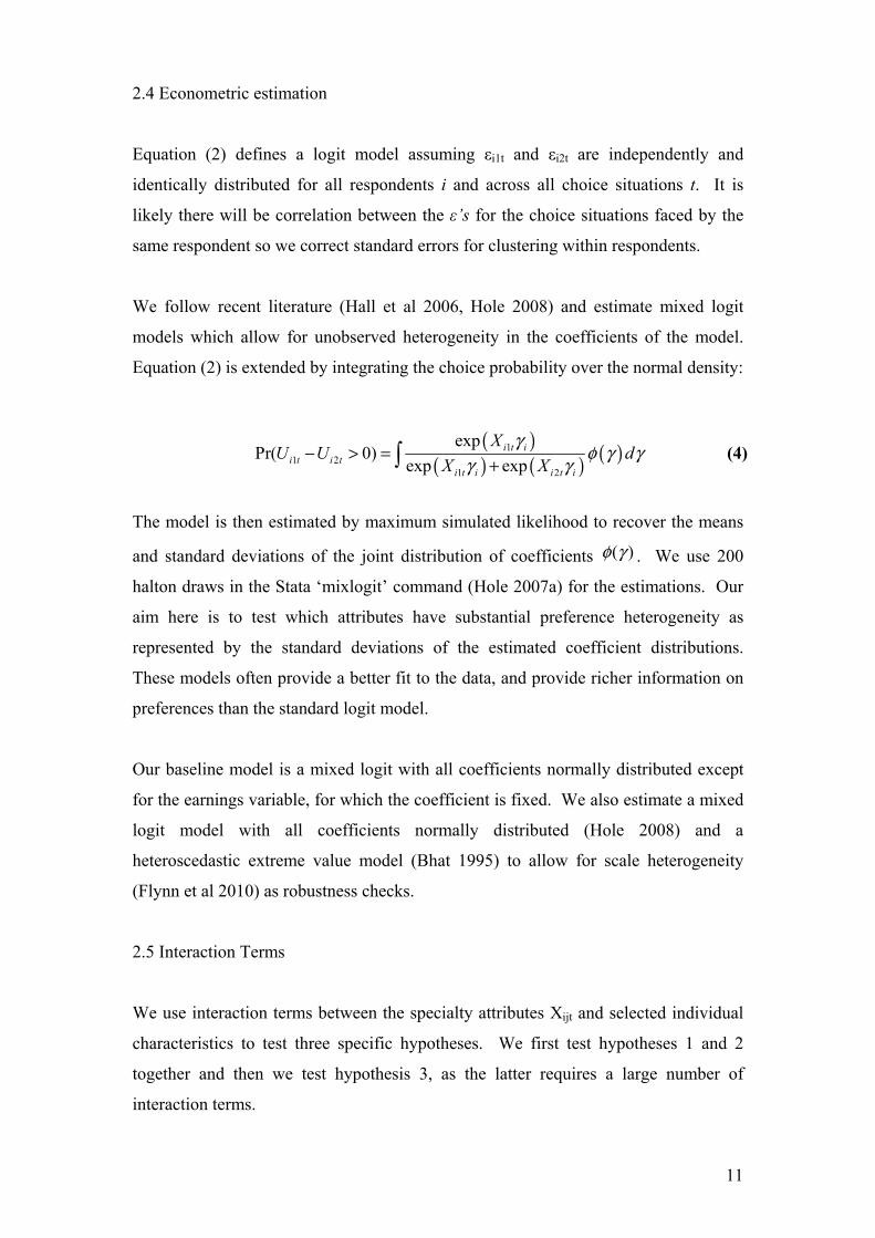
2.4 Econometric estimation

Equation (2) defines a logit model assuming εi1t and εi2t are independently and

identically distributed for all respondents i and across all choice situations t. It is

likely there will be correlation between the ε’s for the choice situations faced by the

same respondent so we correct standard errors for clustering within respondents.

We follow recent literature (Hall et al 2006, Hole 2008) and estimate mixed logit

models which allow for unobserved heterogeneity in the coefficients of the model.

Equation (2) is extended by integrating the choice probability over the normal density:

( )

( ) ( ) ( )11 2

1 2

expPr( 0)

exp expi t i

i t i ti t i i t i

XU U d

X X

γφ γ γ

γ γ− > =

+ (4)

The model is then estimated by maximum simulated likelihood to recover the means

and standard deviations of the joint distribution of coefficients ( )φ γ . We use 200

halton draws in the Stata ‘mixlogit’ command (Hole 2007a) for the estimations. Our

aim here is to test which attributes have substantial preference heterogeneity as

represented by the standard deviations of the estimated coefficient distributions.

These models often provide a better fit to the data, and provide richer information on

preferences than the standard logit model.

Our baseline model is a mixed logit with all coefficients normally distributed except

for the earnings variable, for which the coefficient is fixed. We also estimate a mixed

logit model with all coefficients normally distributed (Hole 2008) and a

heteroscedastic extreme value model (Bhat 1995) to allow for scale heterogeneity

(Flynn et al 2010) as robustness checks.

2.5 Interaction Terms

We use interaction terms between the specialty attributes Xijt and selected individual

characteristics to test three specific hypotheses. We first test hypotheses 1 and 2

together and then we test hypothesis 3, as the latter requires a large number of

interaction terms.

11

Hypothesis 1: DITs with high levels of educational debt will value future earnings

more highly

This hypothesis is informed by the US literature on specialty choice which finds that

educational debt is an important factor (Thornton 2000, Nicolson 2002). In the light

of these findings it is important to see if educational debt also plays a role in a country

like Australia, where university education is more heavily subsidized.

To test the hypothesis we interact the level of educational debt with the earning

attribute in the multinomial logit model. The relevant question in MABEL is: “What

is the total level of financial debt that you currently have as a result of your medical

education and training? (Give dollar amount; include HECS debt, other debt

associated with training and living expenses)”. The Higher Education Contribution

Scheme (HECS) is the main government-run student loan and repayment system in

Australia. We use the continuous debt variable as an interaction as higher debt levels

are likely to have larger effects on valuation of earnings.

Hypothesis 2: Female doctors and doctors with children will value flexibility of hours

worked more highly

Harris et al (2005) find that “Factors of particular importance to women, compared

with men, were “appraisal of domestic circumstances” (odds ratio, 1.9), “hours of

work” (OR, 1.8) and “opportunity to work flexible hours” (OR, 2.6)” in a

retrospective study of specialty choice. Flexible hours may be more important for

women is that they often take a majority role in childcare. As MABEL also has

detailed information on domestic circumstances, including children in the family, we

also test for the effect of having children in the family (for male and female doctors).

To test this hypothesis we interact two dummy variables: “Female” and “Children”

(=1 if the doctor reports having any children) with the “Change in hours” and

“Control over hours” attributes.

12

Hypothesis 3: Personality affects work/life preferences for DITs

Personality is of increasing interest to economists looking to explain individuals’

employment and life outcomes (Borghans et al 2008). One is example is that

extroverted workers may select into jobs with more social interactions (Kruger and

Schkade 2008). We might expect extroverted doctors to prefer continuity of care,

which require repeated interactions with patients and good communication skills.

Information on the ‘big five’ personality characteristics (openness, conscientiousness,

extraversion, agreeableness and neuroticism) was collected in Wave 2 of MABEL

(the year after the DCE) and was merged back into Wave 1 for returning respondents

(personality data is available for approximately 58 % of respondents in our sample).

We interact de-meaned and standardized variables for each of the ‘big five’

characteristics with all attributes in the DCE as we have no prior expectation about

which attributes may be most sensitive to personality differences.

3. Results

The MABEL response rate for “hospital non-specialists” is 16.45% from a sampling

frame of 8,820 giving 1,451 respondents. After excluding pilot respondents and

CMOs we have 536 respondents of which 532 answer at least one DCE question. The

estimation sample is 4808 observations from 532 junior doctors. Table 2 presents

descriptive statistics on some basic variables available in the MABEL survey data as

well as variables used for interactions. We can see the sample is young (29 years old

on average) and a small majority (62%) are female. These figures show MABEL

respondents are slightly younger and more respondents are female compared to the

most comprehensive estimate of the population age (30 years) and gender (52%

female) (AIHW 2009). Compared to older, fully qualified GPs and specialists,

average income is quite low, and hours worked about 3 hours/week higher (Joyce et al

2010). A small proportion of doctors have children (12%), and the mean educational

debt is $27,710.

[Insert Table 2 about here]

13

Table 3 reports estimates for the MNL and MXL models with standard errors

clustered by respondent. For both models we present the Bayesian Information

Criterion (BIC=-2logL+ k*ln(n)) where logL is the log-likelihood, k is the number of

parameters estimated and n is the number of observations.

[Insert Table 3 about here]

In the MNL model, the estimated coefficients are statistically significant at 1% for all

attributes apart from “Continuity of care - Regularly”. The estimated coefficients all

have the expected sign, and for the attributes with three dummy-coded levels, utility is

estimated to be monotonically increasing in the attribute. Doctors prefer lower hours

of work, high control over hours, low on-call, excellent academic opportunities, and

high levels of procedural work.

The MXL model coefficient means are all approximately 50% greater then the

coefficient point-estimates in the MNL model. All but one of the coefficient

distributions have substantial and statistically significant standard deviations. This

suggests that there is substantial preference heterogeneity over the attributes. The

lower BIC in the MXL indicates this model is preferred in terms of model ‘fit’.

The estimated standard deviations of each coefficient in the MXL model can tell us

the amount of preference heterogeneity across the different attributes. Mostr

attributes have relatively substantial standard deviations. The “On-Call – 1 in 10”

attribute coefficient has a small standard deviation which is not statistically

significant. This indicates most doctors have similar preferences over this attribute, in

this case it has a positive effect on utility; doctors prefer less on-call time. “Change in

hours (%)” also has a relatively small standard deviation (<40% of the coefficient

mean) indicating relatively little variation in preferences over working fewer hours.

Marginal willingness-to-pay (MWTP) values, the marginal rate of substitution

between each attribute and the earnings attribute, are also calculated. We can

interpret these values as the sum of money (in terms of annual income) a doctor

would give up in order to gain a unit increase in the attribute. A negative value

represents an attribute with a negative effect on utility and can be interpreted as the

14

sum of money the doctor would be willing to accept (in terms of annual income) to

compensate for a unit increase in the attribute.

[Insert Table 4 about here]

Table 4 presents MWTP values for models 1 and 2. Standard errors are calculated by

the delta method (Hole, 2007b). The two models have very similar mean values for

most of the attributes, we concentrate on the mean MWTP for the MXL model. First

we discuss the dummy-coded attributes then we return to a detailed analysis of the

change in hours attribute. In general all the specialty attributes have large but

plausible monetary values according to our estimates. An exception is the “On-Call”

attribute which has very high valuations, outside the range of the earnings attribute (in

the case of “On-Call - 1 in 2”). A consistent result is that the higher (‘better’) level of

each attribute is valued less over the medium level, than the medium level is valued

over the lowest level. This finding is consistent with diminishing returns to attributes.

Both work-life and intrinsic specialty attributes have substantial valuations. We

estimate that doctors are willing to accept a $53,000 decrease in annual earnings to

have “Control over hours – Medium” rather than “Control over hours – Low”. A

slightly higher valuation ($62,000) is given to having some procedural work

compared to none. Attributes with lower valuations are “Academic opportunities”

and “Continuity of care”. Both of these attributes have the lower levels valued at

$33,000-$36,000.

The “Change in hours” attribute suggests doctors will trade-off hours worked per

week at $4,109 for a 1% change or $41,088 for a 10% change. Using the figure for

average hours worked from Table 2 we can see 10% = 5 hours. We can convert this

monetary value into a hypothetical marginal wage rate. We have $41,088 / 52 =

$706.41 for a change of 5 hours per week, so we have $790 / 5 = $158.03 per hour.

We can interpret this as the wage at which the average doctor would be prepared to

work an extra hour.

As the MABEL data includes information on earnings and hours for specialists and

GPs, we can compare the wage rate implied by the DCE with the actual hourly wages

15

of specialists and GPs. Cheng et al (2010) show that the average wage for a GP is

$87.10 and for a specialist $135.53. The marginal wage rate implied by the DCE is

slightly higher than the actual wage rates earned by specialists.

Two additional models were estimated as robustness checks: a mixed logit model

allowing the earnings coefficient to be normally distributed and an heteroscedastic

extreme value model. The MWTP values calculated from are both very similar to the

baseline mixed logit results in model (2). Results of these models are omitted for

brevity.

Predicted probability analysis and policy simulation

To learn more about the policy implications of the results we conduct a predicted

probability analysis (Lancsar and Louviere 2008) and policy simulation. This

involves first a simulation of the model (ie calculating predicted probabilities for each

choice) for a plausible real life choice between alternative specialties. Secondly, we

simulate the model after unilateral changes in attributes for one of the alternative

specialties. These changes in attributes can represent government policy changes.

Due to the shortage of GPs in Australia (AMWAC 2005), and internationally

(Bodenheimer et al 2007) we choose to simulate the choice of “General Practitioner”

versus the choice of “Specialist”. For the baseline simulation, we use MABEL data to

inform the attribute levels for the two alternative choices. Where we quote figures in

the following text, they are the raw means of the corresponding variable presented in

Table 5.

For the earnings and hours attributes we have direct measures in MABEL. In terms of

gross earnings, specialists earn on average $334,937 and GPs earn on average

$183,067, a difference of $151,870. For the simulation we set the difference between

the two alternatives to be $100,000, the maximum difference in earnings between

alternative specialties in the choice experiment.

16

For hours worked per week (not including on-call), specialists work 45.4 hours and

GPs 38.8 hours, a difference of 6.6 hours. For the simulation we choose a 17%

difference, as 17% of the GPs 38.8 hours is 6.6 hours.

Evidence from three MABEL variables shows that compared to GPs, specialists are

more likely to be dissatisfied with their hours of work (28% vs 17%), agree that they

can’t take time off when they want to (43 % vs 39%), and have unpredictable hours

(44% vs 21%). Using this evidence in the simulation, we set “Control over hours” to

be “Medium” for GPs and “Low” for specialists.

As GPs see the same patient for multiple medical problems, and due to the

continuous/ongoing nature of primary care for chronic disease and family planning,

GPs provide more continuity of care to their patients than Specialists. In the

simulation, we set “Continuity of care” to be “Sometimes” for Specialists and

“Regularly” for GPs. For “Academic opportunities” there is some evidence in

Australia (Joyce et al 2009) that more specialists than GPs are involved in research

(15% vs 1%), so we set this attribute to “Average” for specialists and “Poor” for GPs.

Using the relevant MABEL question we find that on average GPs are on-call 1 in 7.7

and specialists 1 in 5.9. To relate these to the ratios used in the DCE attribute, for the

simulation we choose On-call to be “1 in 10” for GPs and “1 in 4” for specialists.

Table 6 presents the attribute levels for the simulation and the predicted probabilities

for four simulations of the model. The base case predicts that 46% of doctors will

choose the “GP” option and 54% will choose “Specialist”. The final three rows of the

table show how unilateral changes in three selected attributes for the “GP” alternative

affect the predicted probabilities.

We can see how increasing procedural work to “Some” has the largest effect on

choice probabilities, increasing the number of doctors choosing “GP” from 46% to

62%. Increasing earnings by $50,000 has a slightly smaller effect, increasing the

proportion choosing general practice to 58%. Giving GPs “Average” instead of

“Poor” academic opportunities increases the proportion by only eight percentage

points to 55%. The ranking of the effects of these different attributes corresponds to

17

their ranking according to willingness-to-pay (see Table 4, $65,874, $50,000 and

$35,019).

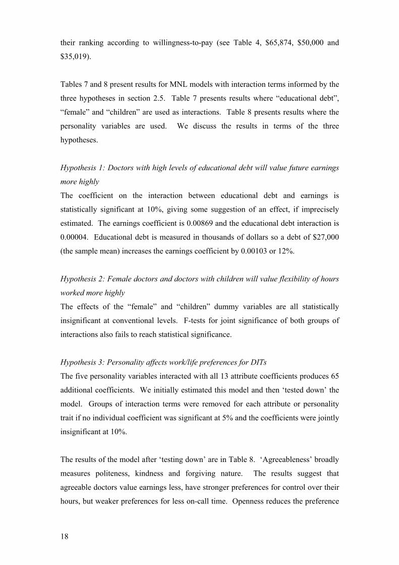
Tables 7 and 8 present results for MNL models with interaction terms informed by the

three hypotheses in section 2.5. Table 7 presents results where “educational debt”,

“female” and “children” are used as interactions. Table 8 presents results where the

personality variables are used. We discuss the results in terms of the three

hypotheses.

Hypothesis 1: Doctors with high levels of educational debt will value future earnings

more highly

The coefficient on the interaction between educational debt and earnings is

statistically significant at 10%, giving some suggestion of an effect, if imprecisely

estimated. The earnings coefficient is 0.00869 and the educational debt interaction is

0.00004. Educational debt is measured in thousands of dollars so a debt of $27,000

(the sample mean) increases the earnings coefficient by 0.00103 or 12%.

Hypothesis 2: Female doctors and doctors with children will value flexibility of hours

worked more highly

The effects of the “female” and “children” dummy variables are all statistically

insignificant at conventional levels. F-tests for joint significance of both groups of

interactions also fails to reach statistical significance.

Hypothesis 3: Personality affects work/life preferences for DITs

The five personality variables interacted with all 13 attribute coefficients produces 65

additional coefficients. We initially estimated this model and then ‘tested down’ the

model. Groups of interaction terms were removed for each attribute or personality

trait if no individual coefficient was significant at 5% and the coefficients were jointly

insignificant at 10%.

The results of the model after ‘testing down’ are in Table 8. ‘Agreeableness’ broadly

measures politeness, kindness and forgiving nature. The results suggest that

agreeable doctors value earnings less, have stronger preferences for control over their

hours, but weaker preferences for less on-call time. Openness reduces the preference

18

for control over hours but increases the preference for less on-call working whereas

the ‘extraversion’ trait only has a statistically significant effect on the procedural work

coefficient. The preference for ‘enough’ procedural work is reduced to near zero by a

one standard-deviation increase in extraversion. The results suggest neurotic doctors

value earnings less, control over hours more, continuity of care more and procedural

work less.

4. Discussion

This study shows that a range of work-life and intrinsic job attributes influence choice

of specialty for junior doctors. The results suggest doctors would be prepared to

sacrifice substantial proportions of their annual income (20 to 25% based on an

annual income of $200,000) for improvements in control over working hours and

opportunities to do procedural work. The most highly valued attribute is time spent

On-Call, where avoiding being on call every other day had a valuation nearly twice as

high as any other attribute (approximately 50% of annual income).

Our finding that the average hourly wage implied by our coefficient estimates

($158.03) is a similar magnitude to the actual average hourly wage of specialists in

MABEL ($135.53, Cheng et al 2010) adds credibility to our results. It also provides

evidence of a gap between the earnings expectations of doctors and the average

hourly wage of GPs ($87.10). The earnings gap is a common explanation for

oversupply of specialists and undersupply of GPs (Bodenheimer et al 2007).

One caveat to this finding is that in interpreting these values we must recognize how

the choice of levels for the earnings attribute could influence estimated valuations

(Skjoldborg and Gyrd-Hansen 2003). As we have chosen a relatively wide range for

earnings ($150,000 to $250,000), we may expect this to provide lower valuations for

earnings, or equivalently high monetary valuations of other attributes, including hours

worked. However, our choice of levels was informed by evidence, and also relate to

expected future earnings, and hence the relatively wide range.

The simulations can be used to see how changes in attributes of GP working

conditions may influence the future GP workforce. Our simulation predicts a baseline

19

probability of choosing ‘GP’ of 39% that rises by 16 percentage points with an

increase in procedural work or 12 percentage points for a 1/3 ($50,000) increase in

earnings. Increasing academic opportunities to ‘Average’ increases the probability 9

percentage points. Data from the Australian Medical Training Review Panel 2010

(Medical Training Review Panel 2010) shows that in 2009 there were 2,352 junior

doctors commencing the second year of postgraduate training in Australia. In the

same year, there were 938 first-year GP trainee positions available, projected to

increase to 1200 by 2014 (RACGP 2010). An increase of 9, 12, or 16 percentage

points as suggested by our simulation is equivalent to 212, 282 or 376 extra doctors

choosing to enroll as GP registrars every year.

Previous revealed preference studies from the US have suggested educational debt

influences specialty choice through a preference for higher earnings (Thornton 2000,

Nicolson 2002). Our results give some weak support to this hypothesis in a different

context where educational debt is not as high. In contrast, we have not been able to

corroborate previous research from Australia suggesting female doctors or doctors

with children have a higher valuation of flexible working hours and shorter working

hours (Harris et al 2005). As only 12% of doctors in our sample have children, these

family reasons may be less important for junior doctors.

This paper is unique among DCEs concerned with medical labour markets in allowing

measures of personality traits to affect the valuation of attributes, and the impact of

personality on specialty choice. Our finding that extraverted doctors have a much

lower (or zero) valuation of procedural work is related to the finding that extraverted

workers self-select into jobs with more social interactions (Krueger and Schkade

2008). This implies that extraverted doctors are more likely to select general practice

as a specialty. However we did not find the expected interaction between

extraversion and continuity of care. The finding that neurotic and agreeable doctors

have a lower preference for earnings matches with the conclusions from a study

which finds both neurotic and agreeable individuals suffer an earnings penalty

compared to other workers (Mueller and Plug 2006).

In addition to the average valuations of specialty attributes and interactions with

observable characteristics, this paper also provides information about unobservable

20

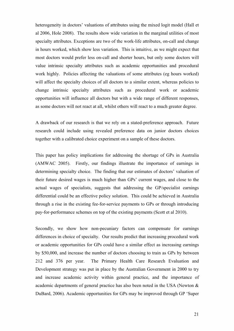
heterogeneity in doctors’ valuations of attributes using the mixed logit model (Hall et

al 2006, Hole 2008). The results show wide variation in the marginal utilities of most

specialty attributes. Exceptions are two of the work-life attributes, on-call and change

in hours worked, which show less variation. This is intuitive, as we might expect that

most doctors would prefer less on-call and shorter hours, but only some doctors will

value intrinsic specialty attributes such as academic opportunities and procedural

work highly. Policies affecting the valuations of some attributes (eg hours worked)

will affect the specialty choices of all doctors to a similar extent, whereas policies to

change intrinsic specialty attributes such as procedural work or academic

opportunities will influence all doctors but with a wide range of different responses,

as some doctors will not react at all, whilst others will react to a much greater degree.

A drawback of our research is that we rely on a stated-preference approach. Future

research could include using revealed preference data on junior doctors choices

together with a calibrated choice experiment on a sample of these doctors.

This paper has policy implications for addressing the shortage of GPs in Australia

(AMWAC 2005). Firstly, our findings illustrate the importance of earnings in

determining specialty choice. The finding that our estimates of doctors’ valuation of

their future desired wages is much higher than GPs’ current wages, and close to the

actual wages of specialists, suggests that addressing the GP/specialist earnings

differential could be an effective policy solution. This could be achieved in Australia

through a rise in the existing fee-for-service payments to GPs or through introducing

pay-for-performance schemes on top of the existing payments (Scott et al 2010).

Secondly, we show how non-pecuniary factors can compensate for earnings

differences in choice of specialty. Our results predict that increasing procedural work

or academic opportunities for GPs could have a similar effect as increasing earnings

by $50,000, and increase the number of doctors choosing to train as GPs by between

212 and 376 per year. The Primary Health Care Research Evaluation and

Development strategy was put in place by the Australian Government in 2000 to try

and increase academic activity within general practice, and the importance of

academic departments of general practice has also been noted in the USA (Newton &

DuBard, 2006). Academic opportunities for GPs may be improved through GP ‘Super

21

Clinics’ linked to Universities (Dart et al 2010). Our findings highlight the importance

of such initiatives for recruitment to the general practice workforce.

The reality that much of general practice is non-procedural (Baron, 2010) sits

uncomfortably with our finding that young doctors prefer more procedural work.

Doctors’ preference for procedural work may be related to the fact that fee-for-service

payment models generally remunerate procedures better than non-procedural activity.

In recent years in Australia, many GPs have ceased traditional areas of procedural

practice, such as obstetrics, and it may be that strategies to better support these

activities (for example, changed medical indemnity insurance arrangements) would

enhance the attractiveness of general practice. Somewhat ironically, Australian GPs

in rural areas often undertake more procedural work than their metropolitan

colleagues, and this feature could be used to enhance recruitment into these regions,

which have long suffered from workforce shortages.

22

References Australian Bureau of Statistics (2002). Private Medical Practitioner. Report No. 8689.0. Canberra: ABS Australian Institute of Health and Welfare (2009). National health labour force series. Medical labour force 2007. Canberra: AIHW Australian Medical Workforce Advisory Committee (2005). Career Decision Making by Postgraduate Doctors. AMWAC Report 2005.3. [available from http://www.ahwo.gov.au/documents/Publications/2005/Career%20decision%20making%20by%20postgraduate%20doctors%20-%20%20Key%20findings.pdf, accessed 09/09/2010] Baron, R.J. (2009). The chasm between intention and achievement in primary care. JAMA. 301(18):1922-1924. Bhat, C.R., (1995). A heteroscedastic extreme value model of intercity travel mode choice. Transportation Research Part B 29 (6): 471-483 Blamey, R.K., Bennett, J.W., Louviere, J.J., Morrison, M.D., & Rolfe, J. (2000). A test of policy labels in environmental choice modelling studies. Ecological Economics 32(2): 269-286 Bodenheimer, T., Berenson, R.A., & Rudolf, P. (2007). The primary care-specialty income gap: Why it matters. Annals of Internal Medicine 146:301-306 Borghans, L., Duckworth, A. L., Heckman, J. J., & ter Weel, B. (2008). The economics and psychology of personality traits. Journal of Human Resources 43 (4): 972-1059 Carlsson, F., & Martinsson, P. (2003). Design techniques for stated preference methods in health economics. Health Economics 12: 281 – 294. Cheng, T.C., Scott, A., Jeon, S.H., Kalb, G., Humphreys, J., & Joyce, C. (2010). What factors influence the earnings of GPs and medical specialists in Australia? Evidence from the MABEL survey. Melbourne Institute Working Paper 12/10. Melbourne: University of Melbourne Dart, J.M., Jackson C.L., Chenery, H.J., Shaw, P.N., & Wilkinson, P. (2010). Meeting local complex health needs by building the capacity of general practice: the University of Queensland GP super clinic model. Medical Journal of Australia 193 (2): 86-89 De Bekker-Grob, E.W., Hol, L., Donkers, B., Van Dam, L., Habbema, J.D.F., van Leerdam, M.E., Kulpers, E.J., Essink-Bot, M.L., & Steyerberg, E.W. (2010). Labeled versus unlabeled discrete choice experiments in health economics: an application to colorectal cancer screening. Value in Health 13 (2): 315-323

23

Dorsey, E.R., Jarjoura, D., & Rutecki, G.W., (2003). Influence of controllable lifestyle on recent trends in specialty choice by US medical students. JAMA 290 (9):1173-1178 Dowton, S.B., Stokes, M., Rawstron, E.J., Pogson, P.R., & Brown, M.A. (2005). Postgraduate medical education: rethinking and integrating a complex landscape. Medical Journal of Australia, 182:177-180 Flynn, T.N., Louviere, J.J., Peters, T.J., Coast, J. (2010). Using discrete choice experiments to understand preferences for quality of life. Variance-scale heterogeneity matters. Social Science and Medicine 70 (12): 1957-1965 Gagne, R., & Leger, P.T. (2005). Determinants of physicians’ decisions to specialize. Health Economics 14: 721-735 Hall, J., Fiebig, D.G., King, M.T., Hossain, I., Louviere, J.J. (2006). What influences participation in genetic carrier testing? Results from a discrete choice experiment. Journal of Health Economics, 2006;25(3):520-537. Harris, M.G., Gavel, P.H., & Young, J.R. (2005). Factors influencing the choice of specialty of Australian medical graduates. Medical Journal of Australia 183(6): 295 – 300. Hole, A. R. (2007a). Fitting mixed logit models by using maximum simulated likelihood. Stata Journal, 7(3): 388-401. Hole, A. R. (2007b). A comparison of approaches to estimating confidence intervals for willingness to pay measures. Health Economics 16 (8): 827-840 Hole, A.R. (2008). Modelling heterogeneity in patients' preferences for the attributes of a general practitioner appointment. Health Economics. 27:1078-1094. Hurley, J. (1991). Physicians’ choices of specialty, location, and mode: A reexamination within an interdependent decision framework. Journal of Human Resources 26 (1): 47-71 Joyce, C.M., & McNeil, J.J. (2006). Fewer medical graduates are choosing general practice: a comparison of four cohorts, 1980–1995. Medical Journal of Australia 185: 102-104 Joyce, C.M., Piterman, L., & Wesselingh, S.L. (2009). The widening gap between clinical, teaching and research work. Medical Journal of Australia. 191:169-172. Joyce, C.M., Scott, A., Jeon, S., Humphreys, J., Kalb, G., Witt, J., & Leahy A. (2010). The “Medicine in Australia: Balancing Employment and Life (MABEL)” longitudinal survey – Protocol and baseline data for a prospective cohort study of Australian doctors’ workforce participation. BMC Health Services Research. 10:50.

24

King, M.T., Hall, J., Lancsar, E., Fiebig, D., Hossain, I., Louviere, J., Reddel, H., & Jenkins, C. (2007). Patient preferences for managing asthma: results from a discrete choice experiment. Health Economics. 16(7):703-17. Kolstad, J.R. (2010). How to make rural jobs more attractive to health workers. Findings from a discrete choice experiment in Tanzania. Health Economics In Press DOI: 10.1002/hec.1581 Krueger, A., & Schkade, D., (2008). Sorting in the labour market: Do gregarious workers flock into interactive jobs? Journal of Human Resources 43(4): 859-883 Kruijshaar, M.E., Essink-Bot, M.L., Donkers, B., Looman, C.W.N., Siersema, P.D., & Steyerberg, E.W. (2009). A labeled discrete choice experiment adds realism to the choices presented: preferences for surveillance tests for Barrett esophagus. BMC Medical Research Methodology 9:31 Kuhfeld, W.F. (2005). Marketing research methods in SAS. Experimental design, choice, conjoint, and graphical techniques. SAS 9.1 Edition TS-722. Lambert, T.W., Goldacre, M.J., & Turner, G. (2006). Career Choices of United Kingdon medical graduates of 2002: questionnaire survey. Medical Education 40: 514-521 Lancsar, E., & Louviere, J. (2008). Conducting discrete choice experiments to inform healthcare decision making. Pharmacoeconomics 26 (8): 661-677 Lasser, K. E., Woolhandler, S., & Himmelstein, D.U. (2008). Sources of US physician income: The contribution of government payments to the specialist-generalist income gap. Journal of General Internal Medicine 23 (9): 1477-1481 Medical Training Review Panel (2010). Thirteenth Report. April 2010 Canberra: Commonwealth of Australia. Mueller, G., & Plug, E. (2006). Estimating the effect of personality on male and female earnings. Industrial and Labour Relations Review 60 (1): 3-22 Newton, W.P., & DuBard C.A. (2006). Shaping the future of academic health centers: the potential contribution of departments of family medicine. Annals of Family Medicine. 4 Suppl 1: S2-S11. Nicholson, S. (2002). Physician Specialty Choice under Uncertainty. Journal of Labor Economics 20 (4):816-847 Productivity Commission (2005). Australia’s Health Workforce. Research Report, Canberra: Commonwealth of Australia Royal Australian College of General Practitioners (2010). Federal Budget recognises the central role of general practice. Media Release 11 May [available from http://www.racgp.org.au/media2010/37442 accessed 09/09/2010]

25

Ryan, M., & Skatun D. (2004). Modelling non-demanders in choice experiments. Health Economics 13, 397-402. Scott, A. (2001). Eliciting GPs’ preferences for pecuniary and non-pecuniary job characteristics. Journal of Health Economics 20: 329 – 347. Scott, A., Naccarella, L., Furler, J., Young, D., Sivey, P., Ait Ouakrim, D., & Willenberg, L. (2010). Using financial incentives to improve the quality of primary care in Australia. Report to Australian Primary Health Care Research Institute, Canberra: Australian National University. Sloan, F. (1970). Lifetime earnings and physicians choice of specialty. Industrial and Labour Relations Review 24 (1): 47-56 Skjoldborg, U.S., and Gyrd-Hansen, D. (2003). Conjoint analysis. The cost variable: an Achilles’ heel? Health Economics 12: 479 – 491. Stokes, T., Tarrant, C., Mainous, A.G. 3rd, Schers, H., Freeman, G. & Baker R. (2005). Continuity of care: is the personal doctor still important? A survey of general practitioners and family physicians in England and Wales, the United States, and The Netherlands. Annals of Family Medicine 3(4): 353 – 359. Thornton, J. (2000). Physician choice of medical specialty: do economic incentives matter? Applied Economics 32(11): 1419-1428 Ubach, C., Scott, A., French, F., Awramenko, M., & Needham, G. (2003). What do hospital consultants value about their jobs? A discrete choice experiment. British Medical Journal 326: 1432 – 1437. Zwerina, K., Huber, J., & Kuhfeld, W. (1996). A general method for constructing efficient choice designs. Working Paper, Fuqua School of Business, Duke University.

26

Figure 1: Doctor training in Australia

Figure 2: Example of the DCE preamble and question

Medical Degree (6 Yrs)

Intern (1 Year)

General practice registrar (3 years)

Resident / Hospital Medical O

(up to 3 yrs

fficer

)

Specialist training programs (3 to 6 years)

Career Medical Officer

Source: adapted from Dowton et al 2006 and Productivity Commission, 2005

Choice of specialty training program

Medical registration

27

Table 1: Specialty attributes and levels Specialty attribute Levels

Expected average annual earnings $150,000 $200,000* $250,000 Change in total hours worked 10% more The same* 10% less Control over hours Low Medium* High On-call arrangements 1 in 2 1 in 4* 1 in 4 – infrequently called out 1 in 10 Opportunities for procedural work None Some* Enough Academic/Research opportunities Poor Average* Excellent Continuity of care (see patients more than once)

Rarely

Sometimes* Regularly

Notes: * indicates reference category

Table 2: Descriptive Statistics

Obs Mean S.D. Age 528 28.782 4.643 Female 532 0.615 0.487 Children (>0) 532 0.124 0.330 Educational Debt ('000 AUD) 532 27.710 35.226 Income (Gross AUD per year) 286 73161 38391 Hours/week 476 50.046 11.613 Position: Intern 532 0.180 0.385 HMO yr 1 532 0.306 0.461 HMO yr 2 532 0.299 0.458 HMO yr 3 532 0.214 0.411

28

Table 3: MNL and MXL model results

(1) MNL (2) MXL

Attribute

Coeff. (S.E.)

Coeff. (S.E.)

S.D. (S.E.)

Earnings ($’000) 0.010*** (0.001)

0.015*** (0.001)

Change in hours (%) -0.040*** (0.003)

-0.061*** (0.006)

-0.024** (0.009)

Control hours - High 0.206*** (0.057)

0.302*** (0.086)

0.634*** (0.166)

Control hours - Low -0.525*** (0.053)

-0.777*** (0.081)

-0.533*** (0.152)

On-Call - 1 in 10 0.713*** (0.070)

1.056*** (0.111)

0.088 (0.448)

On-Call - 1 in 2 -1.097*** (0.071)

-1.638*** (0.126)

0.888*** (0.201)

On-Call - 1 in 4 infrequent 0.602*** (0.071)

0.934*** (0.116)

0.939*** (0.129)

Academic - Excellent 0.240*** (0.049)

0.303*** (0.073)

0.707*** (0.141)

Academic - Poor -0.333*** (0.053)

-0.524*** (0.082)

0.804*** (0.120)

Continuity - Rarely -0.312*** (0.058)

-0.430*** (0.087)

0.542*** (0.141)

Continuity - Regularly 0.058 (0.062)

0.115 (0.089)

0.732*** (0.133)

Procedural - Enough 0.209*** (0.050)

0.303*** (0.074)

-0.505*** (0.134)

Procedural - None -0.601*** (0.059)

-0.918*** (0.097)

1.000*** (0.138)

Log L -2617.29 -2520.88 BIC 5344.788 5253.71

Obs 4808 4808

Notes: Model (1): Multinomial logit (MNL),Model (2) Mixed Logit (MXL). Model (2) assumes normal distribution for all attributes except earnings. Standard errors are corrected for clustering at respondent level. Reference category is Control over hours - Medium, On-Call - 1 in 4, Academic - Average, Continuity - Sometimes, Procedural - Some.

29

Table 4: Marginal willingness-to-pay (annual $'000) for changes in specialty attributes

(1) MNL (2) MXL

Attribute Point-estimate

Mean S.D. Interquartile range

Change in hours (%) -4.22*** (0.43)

-4.11*** (0.41)

-1.60*** (0.61)

[-0.01, 1.02]

Control hours - High 21.53*** (5.88)

20.46*** (5.68)

42.96*** (10.76)

[-1.58, 16.44]

Control hours - Low -54.75*** (7.00)

-52.68*** (6.49)

-36.14*** (9.88)

[-0.17, 16.36]

On-Call - 1 in 10 74.40*** (8.87)

71.57*** (8.22)

5.96 (30.26)

[-12.20, 38.48]

On-Call - 1 in 2 -114.53*** (9.55)

-111.02*** (8.82)

60.19*** (13.71)

[-0.43, 22.53]

On-Call - 1 in 4 infrequent 62.87*** (8.57)

63.33*** (8.46)

63.64*** (8.28)

[2.88, 16.75]

Academic - Excellent 25.02*** (5.64)

20.56*** (5.30)

47.92*** (9.04)

[-0.80, 14.33]

Academic - Poor -34.72*** (5.71)

-35.53*** (5.46)

54.49*** (7.90)

[0.13, 13.35]

Continuity - Rarely -32.59*** (6.90)

-29.16*** (6.32)

36.73*** (9.30)

[0.04, 15.62]

Continuity - Regularly 6.02 (6.38)

7.83 (5.97)

49.62*** (9.26)

[-0.28, 15.24]

Procedural - Enough 21.81*** (5.44)

20.54*** (5.11)

-34.22*** (8.92)

[-0.91, 14.02]

Procedural - None -62.67*** (7.15)

-62.21*** (6.86)

67.77*** (9.66)

[0.35, 16.52]

30

Table 5: Mean values of MABEL variables used to inform simulations

Variable GP Specialist

Earnings (gross annual $AUD) 183067 334937

Hours/week 38.8 45.4

Hours of work: very/moderately dissatisfied

0.17 0.28

It is difficult to take time off when I want to: strongly agree

0.39 0.43

The hours I work are unpredictable: agree

0.21 0.44

On-call Ratio 7.66 5.87

Table 6: Model simulations from Model (2)

Attribute GP Specialist Earnings $150,000 $250,000 Change in hours 0 17% Control over hours Medium Low On-Call 1 in 10 1 in 4 Academic Poor Average Continuity Regularly Sometimes Procedural work None Enough

Change in GP attribute Pr(GP) Pr(Specialist)

Base case (no change) 0.458 0.542

Increase procedural work to "Some" 0.620 0.380

Increase earnings to $200,000 0.580 0.420

Increase academic opps to “Average” 0.549 0.451

31

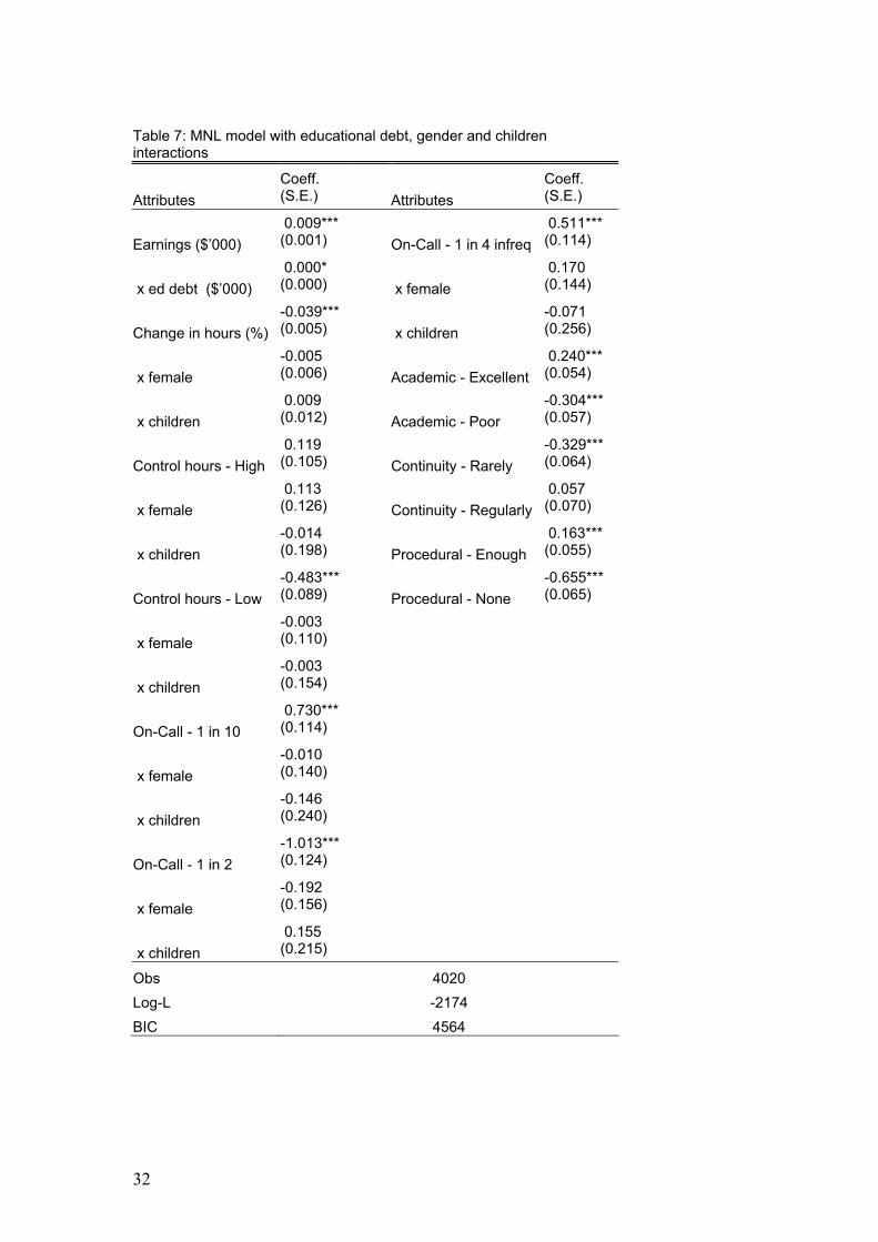
Table 7: MNL model with educational debt, gender and children interactions

Attributes

Coeff. (S.E.)

Attributes

Coeff. (S.E.)

Earnings ($’000)

0.009*** (0.001) On-Call - 1 in 4 infreq

0.511*** (0.114)

x ed debt ($’000)

0.000* (0.000) x female

0.170 (0.144)

Change in hours (%)

-0.039*** (0.005) x children

-0.071 (0.256)

x female

-0.005 (0.006) Academic - Excellent

0.240*** (0.054)

x children

0.009 (0.012) Academic - Poor

-0.304*** (0.057)

Control hours - High

0.119 (0.105) Continuity - Rarely

-0.329*** (0.064)

x female

0.113 (0.126) Continuity - Regularly

0.057 (0.070)

x children

-0.014 (0.198) Procedural - Enough

0.163*** (0.055)

Control hours - Low

-0.483*** (0.089) Procedural - None

-0.655*** (0.065)

x female

-0.003 (0.110)

x children

-0.003 (0.154)

On-Call - 1 in 10

0.730*** (0.114)

x female

-0.010 (0.140)

x children

-0.146 (0.240)

On-Call - 1 in 2

-1.013*** (0.124)

x female

-0.192 (0.156)

x children

0.155 (0.215)

Obs 4020

Log-L -2174

BIC 4564

32

33

Table 8: MNL model with personality interactions

Variable Coeff. (S.E.)

Variable

Coeff. (S.E.)

Earnings ($’000) 0.009*** (0.001)

On-Call - 1 in 2

-1.069*** (0.096)

x agreeableness -0.003*** (0.001)

On-Call - 1 in 4 infrequent 0.658*** (0.095)

x openness 0.001 (0.001)

Academic - Excellent 0.224*** (0.066)

x extraversion -0.001 (0.001)

Academic - Poor -0.371*** (0.070)

x neuroticism -0.002*** (0.001)

Continuity - Rarely -0.341*** (0.075)

Change in hours (%) -0.043*** (0.004)

x agreeableness -0.066 (0.059)

Control hours - High 0.170** (0.076)

x openness 0.003 (0.059)

x agreeableness 0.002 (0.075)

x extraversion -0.090 (0.060)

x openness 0.044 (0.082)

x neuroticism -0.107* (0.062)

x extraversion 0.105 (0.078)

Continuity - Regularly 0.044 (0.082)

x neuroticism -0.058 (0.084)

Procedural - Enough 0.138** (0.066)

Control hours - Low -0.473*** (0.067)

x agreeableness 0.060 (0.064)

x agreeableness -0.132** (0.062)

x openness 0.121* (0.065)

x openness 0.136* (0.071)

x extraversion -0.151** (0.062)

x extraversion 0.073 (0.065)

x neuroticism -0.004 (0.062)

x neuroticism -0.112* (0.066)

Procedural - None -0.633*** (0.079)

On-Call - 1 in 10 0.724*** (0.092)

x agreeableness -0.001 (0.085)

x agreeableness -0.172*** (0.064)

x openness 0.100 (0.084)

x openness 0.116* (0.070)

x extraversion -0.090 (0.079)

x extraversion 0.020 (0.074)

x neuroticism 0.274*** (0.081)

x neuroticism -0.031 (0.061)

Obs 2789 Log-L -2579.6171 BIC 5485