Melbourne-Brisbane Inland Rail Alignment Study 2010 Report.pdf · 6.3 Corridor reservation ......
115
Melbourne–Brisbane Inland Rail Alignment Study Final Report July 2010
Transcript of Melbourne-Brisbane Inland Rail Alignment Study 2010 Report.pdf · 6.3 Corridor reservation ......

Melbourne–BrisbaneInland Rail Alignment StudyFinal ReportJuly 2010

Melbourne–BrisbaneInland Rail Alignment StudyFinal ReportJuly 2010
Photos in this report are included only as illustrations. They do not imply that operating companies whose trains are depicted would use the inland railway.

ARTC Melbourne–Brisbane Inland Rail Alignment Study – Final Report
i
Contents
1. Introduction ................................................................................................. 1
1.1 Terms of reference ................................................................................................................ 3
1.2 The three stages of working papers ...................................................................................... 4
2. Approach to the study ................................................................................. 7
A. Market take up .......................................................................................... 8
3. Demand for Inland Rail ................................................................................ 9
3.1 Freight in the inland railway corridor (all modes) ...................................................................... 9
3.2 Modal analysis methodology ................................................................................................ 10
3.2.1 Price and service attributes assumed........................................................................ 11
3.3 Capacity constraints in the base case .................................................................................. 15
3.4 Demand results .................................................................................................................... 15
B. Route development and costing ........................................................... 26
4. Performance specification and design standards ....................................... 27
4.1 Higher standard ................................................................................................................... 27
4.2 Current Class 1 standards.................................................................................................... 27
4.3 Future proofing .................................................................................................................... 27
4.4 Design and performance standards for the inland railway ..................................................... 28
4.4 Single track .......................................................................................................................... 29
4.4 Track categories ................................................................................................................... 29
5. The route ................................................................................................... 31
5.1 Inland Rail route options ....................................................................................................... 31
5.2 Identification of the route ...................................................................................................... 31
5.2.1 Evaluation of route options........................................................................................ 33
5.2.2 Determination of an end-to-end route ....................................................................... 37
5.3 Analysis of the short-listed routes ......................................................................................... 39
5.3.1 Evaluation of deviations ............................................................................................ 39
5.3.2 Comparison of the routes ......................................................................................... 40
5.4 Developing the final alignment .............................................................................................. 40
5.4.1 Refining the alignment .............................................................................................. 40
5.4.2 Track duplication or dual gauge ................................................................................ 40
5.4.3 The route approaching Brisbane ............................................................................... 41
5.4.4 Summary of proposed alignment .............................................................................. 42
6. Environment and planning ......................................................................... 45
6.1 Preliminary environmental assessment ................................................................................. 45
6.1.1 Development of the proposed alignment................................................................... 45
6.1.2 Environmental risk assessment ................................................................................ 45
6.1.3 Environmental assessment methodology .................................................................. 45

ARTC Melbourne–Brisbane Inland Rail Alignment Study – Final Report
ii
6.1.4 Key environmental impacts ...................................................................................... 45
6.2 Planning approvals strategy ................................................................................................. 46
6.2.1 Overview .................................................................................................................. 46
6.2.2 Approvals delivery framework ................................................................................... 46
6.2.3 Key strategies ........................................................................................................... 48
6.3 Corridor reservation ............................................................................................................. 48
7. Delivery program and capital cost .............................................................. 51
7.1 Staging options .................................................................................................................... 51
7.1.1 Overview .................................................................................................................. 51
7.1.2 Operation via Werris Creek ....................................................................................... 51
7.1.3 Staging of upgrades and Illabo to Stockinbingal deviation ......................................... 51
7.1.4 Toowoomba termination ........................................................................................... 51
7.1.5 Outcome .................................................................................................................. 51
7.2 Delivery program .................................................................................................................. 52
7.3 Capital cost estimate ........................................................................................................... 53
7.3.1 Capital cost model .................................................................................................... 53
7.3.2 Base estimate ........................................................................................................... 53
7.3.3 Land acquisition ....................................................................................................... 54
7.3.4 Risk assessment....................................................................................................... 54
7.3.5 Capital cost .............................................................................................................. 54
8. Operating cost of infrastructure .....................................................................57
8.1 Methodology ........................................................................................................................ 57
8.2 Infrastructure costs .............................................................................................................. 57
8.2.1 Operating costs ........................................................................................................ 57
8.2.2 Signalling system ...................................................................................................... 57
8.2.3 Maintenance costs ................................................................................................... 57
8.2.4 Total infrastructure costs ........................................................................................... 58
8.3 Track access revenue .......................................................................................................... 58
9. Above rail operational benefits ................................................................... 63
9.1 Train operations ................................................................................................................... 63
9.1.1 Journey time results .................................................................................................. 63
9.1.2 Passing loops ........................................................................................................... 63
9.2 Inland Rail train operating costs ........................................................................................... 64
9.2.1 Crew costs ............................................................................................................... 64
9.2.2 Rollingstock maintenance costs ................................................................................ 64
9.2.3 Fuel .......................................................................................................................... 64
9.2.4 Train operating costs ................................................................................................ 64
9.3 Comparison with coastal railway train operating costs (above rail benefits) ........................... 65
C. Financial and economic appraisal .......................................................... 68
10. Financial analysis ....................................................................................... 69
10.1 Financial feasibility ................................................................................................................ 69

ARTC Melbourne–Brisbane Inland Rail Alignment Study – Final Report
iii
10.2 Private and public sector delivery options ............................................................................ 74
10.3 Key issues affecting delivery options .................................................................................... 76
10.3.1 Market appetite for demand based projects .............................................................. 76
10.3.2 Financial markets ...................................................................................................... 76
10.4 Approach to evaluating delivery options .............................................................................. 76
11. Economic analysis ..................................................................................... 79
11.1 Cost benefit analysis methodology ....................................................................................... 80
11.1.1 CBA approach .......................................................................................................... 80
11.1.2 Options considered .................................................................................................. 80
11.1.3 Base case ................................................................................................................ 82
11.1.4 Scenario with Inland Rail ........................................................................................... 86
11.1.5 General CBA assumptions ........................................................................................ 87
11.1.6 Economic costs and benefits .................................................................................... 87
11.2 Outputs/results ................................................................................................................... 89
11.3 Broader economic impacts .................................................................................................. 94
12. Policy issues and delivery strategies .......................................................... 99
12.1 Inland Rail delivery strategies................................................................................................ 99
12.1.1 Private sector involvement/ownership ...................................................................... 99
12.1.2 Treatment of existing infrastructure ......................................................................... 100
12.1.3 Pricing ................................................................................................................... 100
12.1.4 Land reservation .................................................................................................... 101
12.2 Broader policy implications of an inland railway .................................................................. 102
12.2.1 Interface with the coastal railway............................................................................. 102
12.2.2 Broader transport policy ......................................................................................... 102
13. Conclusions ............................................................................................ 105

ARTC Melbourne–Brisbane Inland Rail Alignment Study – Final Report
iv
Contents (continued)
List of tables(Tables 1 to 5 inclusive are contained in the Executive summary, at: http://www.artc.com.au/library/IRAS_Final%20Report%20Executive%20Summary.pdf)
Table 6 Working papers ................................................................................................................... 4
Table 7 Location of Stage 3 working papers in the Final Report ....................................................... 5
Table 8 Characteristics of Melbourne–Brisbane intercapital market ................................................ 11
Table 9 Forecast north and southbound tonnes and net tonne kilometres carried on Inland Rail ........(assuming commencement in 2020) .................................................................................. 22
Table 10 Number of northbound trains per day on Inland Rail (assuming 2020 commencement) ..... 22
Table 11 Melbourne-Brisbane (and backhaul) forecast tonnes (intercapital freight, Base Case and inland railway scenario, assuming Inland Rail commencement in 2020) ..... 23
Table 12 Inland railway performance specifications .......................................................................... 28
Table 13 Proposed track types ........................................................................................................ 42
Table 14 Summary of environmental issues with risk category A ...................................................... 45
Table 15 Summary of capital costs (2010 dollars) ............................................................................. 53
Table 16 Summary of land acquisition costs (2010 dollars) ............................................................... 54
Table 17 Outturn capital cost (2010 dollars) ..................................................................................... 54
Table 18 Operating costs per year (2010 dollars) .............................................................................. 57
Table 19 Maintenance cost per year (2010 dollars) ........................................................................... 57
Table 20 Total Infrastructure cost per year (2010 dollars) .................................................................. 58
Table 21 Inland Rail access revenue assumptions (2010 dollars) ...................................................... 58
Table 22 Average Melbourne to Brisbane journey times ................................................................... 63
Table 23 Inland Rail train operating cost per trip (2010 dollars) ......................................................... 65
Table 24 Inland versus coastal railway train operating costs (2010 dollars) ....................................... 66
Table 25 Financial – project NPV (pre tax) nominal cash flows ($ million, 2010 dollars, discounted, excluding financing costs) .......................................... 70
Table 26 General financial appraisal assumptions ............................................................................. 71
Table 27 Financial sensitivity analysis ($ million, discounted, 2010 dollars) ........................................ 72
Table 28 Delivery options ................................................................................................................. 74
Table 29 Public/private sector funding options ................................................................................ 74
Table 30 Indicative assignment of weightings to criteria .................................................................... 77
Table 31 Indicative scoring scale ...................................................................................................... 77
Table 32 Summary of assumptions for specific scenarios ................................................................. 81
Table 33 ARTC proposed capital spend on the north-south corridor assumed in demand and appraisals ($ millions, undiscounted, 2010 dollars) ...................................................... 84
Table 34 Key economic appraisal assumptions ................................................................................ 87
Table 35 Economic appraisal parameters (2010 dollars) ................................................................... 90
Table 36 Economic – appraisal results for Inland Rail (incremental to the Base Case, $ million, discounted, 2010 dollars) ................................... 91
Table 37 Economic – breakdown of econominc costs and benefits by start date (incremental to the Base Case, $ million, discounted, 2010 dollars) ................................... 91

ARTC Melbourne–Brisbane Inland Rail Alignment Study – Final Report
v
Table 38 Economic sensitivity analysis ($ million, discounted, 2010 dollars) ...................................... 92
Table 39 Estimated construction phase employment (gross FTEs, average per annum over 5-year construction period) ..................................... 94
Table 40 Estimated direct operations phase employment (per annum, FTEs) ................................... 95
List of figures(Figures 1 to 3 inclusive are contained in the Executive summary, at: http://www.artc.com.au/library/IRAS_Final%20Report%20Executive%20Summary.pdf)
Figure 4 Map of the far western sub-corridor.................................................................................... 2
Figure 5 Study approach .................................................................................................................. 7
Figure 6 Components of road and rail price (Melbourne–Brisbane) ....................................................................................................... 12
Figure 7 Aggregate market shares for Melbourne–Brisbane intercapital freight using survey elasticities (no inland railway).................................................................................. 16
Figure 8 Aggregate market shares for Melbourne–Brisbane intercapital freight using survey elasticities (2020 inland railway commencement) ................................................... 17
Figure 9 Freight flows along the corridor related to the inland railway (2050) ................................... 21
Figure 10 Analysis of options in each area ........................................................................................ 31
Figure 11 The main route options for the inland railway .................................................................... 32
Figure 12 Albury and Shepparton route options schematic............................................................... 34
Figure 13 Parkes to Moree route options schematic ......................................................................... 35
Figure 14 Toowoomba and Warwick route options schematic .......................................................... 36
Figure 15 Melbourne to Brisbane route options ................................................................................ 37
Figure 16 Short-listed inland railway routes for analysis .................................................................... 38
Figure 17 Standard and dual gauge corridors ................................................................................... 41
Figure 18 Proposed Inland Rail route ................................................................................................ 43
Figure 19 Approvals delivery framework ........................................................................................... 47
Figure 20 Overall delivery program ................................................................................................... 52
Figure 21 Chart comparing financial sensitivity results for Inland Rail assuming operations commence in 2030 ($ million, discounted, 2010 dollars) ................................................... 73
Figure 22 PFP commercial structure ................................................................................................ 75
Figure 23 Characteristics of the Melbourne-Brisbane road and rail freight market ............................ 82
Figure 24 Alternative road and rail routes between Melbourne and Brisbane ................................... 83
Figure 25 Chart comparing economic sensitivity results for Inland Rail assuming operations commence in 2030 (BCR) ................................................................................................ 93
Figure 26 Cumulative change in selected macroeconomic aggregates due to construction and operation of the inland railway, relative to the Base Case ($ million, discounted, 2010 dollars, assuming Inland Rail commences operations in 2020) ................................ 96

ARTC Melbourne–Brisbane Inland Rail Alignment Study – Final Report
vi
List of boxes
BOX 1 Inland Rail and inland railway ................................................................................................. xii
BOX 2 Terms of reference for the study ............................................................................................. 3
BOX 3 Transit time for the inland railway ......................................................................................... 14
BOX 4 Diversion of freight from road to the inland railway ................................................................ 18
BOX 5 Comparison of demand with more sensitive assumptions .................................................... 24
BOX 6 Single track railway .............................................................................................................. 29
BOX 7 Difference between capital cost estimates ............................................................................ 55
BOX 8 Alternative access prices ...................................................................................................... 59
BOX 9 Financial versus economic evaluation ................................................................................... 79
BOX 10 Potential loss of ARTC revenue .......................................................................................... 103
List of appendices
Appendix A Glossary
Appendix B Market take up
Appendix C Design standards
Appendix D Identification of route options
Appendix E Route development
Appendix F Maps of the proposed alignment
Appendix G Train operations
Appendix H Preliminary environmental assessment
Appendix I Legislation review and planning approvals strategy
Appendix J Capital cost and delivery program
Appendix K Operating cost of infrastructure
Appendix L Financial and economic appraisal methodology
Appendix M Computable and general equilibrium analysis
Appendix N Stakeholders consulted
Appendix O Bibliography and reference list

1. Introduction
1. INTRODuCTIONARTC Melbourne–Brisbane Inland Rail Alignment Study – Final Report

1. INTRODuCTIONARTC Melbourne–Brisbane Inland Rail Alignment Study – Final Report
1
1. IntroductionAn inland route through the Central West of New South Wales (NSW) has the potential to reduce the time it takes to move freight from Melbourne to Brisbane by rail; to increase the capacity of freight rail paths between the two cities; and to avoid Sydney area congestion.
The Melbourne–Brisbane Inland Rail Alignment Study (the study) was announced by the Minister for Infrastructure, Transport, Regional Development and Local Government, the Hon Anthony Albanese MP on 28 March 2008. The study would determine the optimum alignment as well as the economic benefits and likely commercial success of a new standard gauge inland railway between Melbourne and Brisbane. It would provide both the Government and the private sector with information that would help guide future investment decisions, including likely demand and the estimated construction cost of the line, and a range of possible private financing options.
The March 2008 announcement for this study stated that in developing a detailed route alignment, it would generally follow the far western sub-corridor identified by the previous North-South Rail Corridor Study. This sub-corridor is shown on the map below. The North-South Rail Corridor Study commissioned by the Australian Government in September 2005 undertook a high level analysis of various corridors and routes.2
2 Ernst & Young, ACIL Tasman, Hyder 2006, North–South Rail Corridor Study, Executive Report, Commissioned by the Department of Transport and Regional Services, p 9
The Australian Government asked the Australian Rail Track Corporation (ARTC) to conduct the study. ARTC specified and co-ordinated the study’s activities, headed by two lead consultants: Parsons Brinckerhoff (PB) and PricewaterhouseCoopers (PwC). PB engaged Halcrow to support it in alignment development, operations and maintenance costing; Aurecon to support it in engineering and alignment development; Currie and Brown to assist in capital costing; and Davidson Transport Consulting for peer review. PwC engaged ACIL Tasman to undertake volume and demand analysis and support it in economic review, and SAHA for peer review. ARTC staff assisted the study through the provision and review of information.
There were a range of other inputs to the study. A list of parties that have contributed is presented in Appendix N.
Throughout this report, engineering and other references to the physical railway line are termed the ‘inland railway’. The potential business (i.e. the business concept) of financing and operating the railway is referred to in this report as ‘Inland Rail’.
BOX 1 Inland Rail and inland railway

1. INTRODuCTIONARTC Melbourne–Brisbane Inland Rail Alignment Study – Final Report
2
FIGuRE 4 Map of the far western sub-corridor

1. INTRODuCTIONARTC Melbourne–Brisbane Inland Rail Alignment Study – Final Report
3
1.1 Terms of reference
Minister’s announcement
On 28 March 2008, the Minister for Infrastructure, Transport, Regional Development and Local Government, the Hon Anthony Albanese MP announced the study as ‘an open, extensive study to determine the economic benefits and likely success of a new multi-billion dollar standard gauge inland railway between Melbourne and Brisbane’.3
In this announcement, the Minister stated that ARTC was asked to conduct the study, building upon work undertaken earlier in the North-South Rail Corridor Study. The route to be developed would generally follow the far western sub-corridor identified in that study. As well as determining the route alignment, the Minister stated that ARTC study would provide both the Government and private sector with information that will help guide their future investment decisions, including likely demand and an estimated construction cost. The study would provide the Government with a basis for evaluating private financing options for part or the entire project. The Minister also requested that the study be customer-focused and consultative, involving discussions with state governments, industry, local government and major rail customers.
Terms of reference
The terms of reference for the study as announced on 28 March 2008 are presented in Box 2.
BOX 2 Terms of reference for the study
The objectives of the study are to determine:
The optimum alignment of the inland railway, taking into account user requirements and the economic, engineering, statutory planning and environmental constraints. The alignment will be sufficiently proven up so it can be quickly taken through the statutory planning and approval process and into detailed engineering design and construction, should a decision be taken to proceed
The likely order of construction costs +/- 20%
The likely order of below rail (infrastructure) operating and maintenance costs
Above rail operational benefits
The level and degree of certainty of market take up of the alignment
A project development and delivery timetable
A basis for evaluating the level of private sector support for the project.
In developing the detailed alignment for the route, ARTC will generally follow the ‘far western sub-corridor’ identified by the North-South Rail Corridor Study.
The study is to be carried out in three stages, with a review of progress and direction at the end of each stage.
Proposed stages are as follows:
Stage 1 – Determination of the preferred route
Stage 2 – Engineering, environmental and land baseline analysis
Stage 3 – Development of the preferred alignment.
Each of the stages will represent a milestone for the project as a whole. The progress of the study will be reviewed in detail at the end of each stage. Progress to the following stage will be dependent on satisfactory outcomes for the study to date.
Within each stage there will be a series of working papers produced to document the progress of the study. ARTC will consult key interested parties during the study.
3 The Hon Anthony Albanese MP, Minister for Infrastructure, Transport, Regional Development and Local Government 2008, Media Release: Inland Rail Alignment Study Underway, 28 March 2008

1. INTRODuCTIONARTC Melbourne–Brisbane Inland Rail Alignment Study – Final Report
4
1.2 The three stages of working papers
The study has been undertaken over three stages with the work of all the stages brought together in this report.
A series of working papers was produced within each stage. The two lead consultants PB and PwC, in the respective roles of Lead Technical Consultant (LTC) and Financial and Economic Consultant (FEC), were responsible for specific working papers produced at each stage of the study. These papers are presented below.
TABLE 6 Working papers
Stage Working paper Lead responsibility
Stage 1 1 Demand and volume analysis FEC
2 Review of route options LTC
3 Stage 1 Capital works costings LTC
4 Preliminary operating and maintenance cost LTC
5 Stage 1 Economic and financial assessment and identification of the route for further analysis
FEC
Stage 2 6 Design standards LTC
7 Preliminary environmental assessment LTC
8 Preliminary land assessment LTC
10 Development of route LTC
11 Stage 2 Capital works costings LTC
12 Stage 2 Economic and financial analysis FEC
Stage 3 9 Engineering data collection LTC
13 Preliminary environmental assessment LTC
14 Legislation review and planning approvals strategy LTC
15 Refinement of preferred alignments LTC
16 Stage 3 Capital works costings LTC
17 Delivery program LTC
18 Economic and financial assessment FEC
19 Policy issues, options and delivery strategies FEC
The Stages 1 and 2 working papers were published on www.artc.com.au. Their content has been incorporated into the Final Report and appendices or superseded.

1. INTRODuCTIONARTC Melbourne–Brisbane Inland Rail Alignment Study – Final Report
5
The working papers listed as outputs of Stage 3 appear as sections or appendices within this integrated Final Report rather than being published as standalone documents. The table below indicates where the output of Stage 3 working papers can be found in the report.
TABLE 7 Location of Stage 3 working papers in the Final Report
Working paper Location in Final Report
9 Engineering data collection Appendix O
13 Preliminary environmental assessment Chapter 6 and Appendix H
14 Legislation review and planning approvals strategy Chapter 6 and Appendix I
15 Refinement of preferred alignments Chapter 5 and Appendices D, E and F
16 Stage 3 Capital works costings Chapter 7 and Appendix J
17 Delivery program Chapter 7 and Appendix J
18 Economic and financial assessment Chapters 10 and 11 and Appendix L
19 Policy issues, options and delivery strategies Chapters 10 and 12 and Appendix L
2. Approach to the study
2. APPROACH TO THE STuDYARTC Melbourne–Brisbane Inland Rail Alignment Study – Final Report
6

2. APPROACH TO THE STuDYARTC Melbourne–Brisbane Inland Rail Alignment Study – Final Report
7
2. Approach to the studyThe findings contained in this report are based on a combination of market, technical and economic modules. The approach to the study is presented graphically below.
The roadmap provides reference to where information is to be found in the report. While the roadmap suggests a staged process, this is over-simplified as significant interaction and refinement occurred between the modules during the course of the study – for example, performance specifications (Chapter 4) were an input to demand analysis (Chapter 3).
A. Market take up
Whole of corridor freight demand analysis (Chapter 3 and Appendix B)
Survey and interview (Chapter 3 and Appendix B)
Logit model of inland railway relative to other road/rail (Chapter 3 and Appendix B)
Estimate annual tonnes and net tonne kilometres over appraisal period (Chapter 3 and Appendix B)
B. Route development and costing
Performance specification and engineering standards (Chapter 4 and Appendix C)
Assess route options to identify optimum route (Chapter 5 and Appendices D, E and F)
Operational and transit time modelling (Chapter 5 and Appendix G)
Environmental and legislative aspects (Chapter 6 and Appendices H and I)
Capital cost and delivery timetable (Chapter 7 and Appendix J)
Operating cost of infrastructure (Chapter 8 and Appendix K)
Train operating costs (Chapter 9 and Appendix G)
C. Financial and economic analysis
Incorporate demand
Annualise track and train costs and revenues/benefits
Define and estimate Base Case
Analyse financial viability (Chapter 10 and Appendix L)
Analyse economic viability (Chapter 11 and Appendix L)
Policy issues (Chapter 12)
Assess broader impacts (Chapter 11 and Appendix M)
Final Rep
ort
FIGuRE 5 Study approach
Stakeholder consultation and data collection (Appendices N and O)

A. Market take up 3. Demand for Inland Rail
3. DEMAND FOR INLAND RAILARTC Melbourne–Brisbane Inland Rail Alignment Study – Final Report
8

3. DEMAND FOR INLAND RAILARTC Melbourne–Brisbane Inland Rail Alignment Study – Final Report
9
3. Demand for Inland RailThis chapter provides an assessment of demand and potential rail tonnages on the inland railway. The chapter:
Assesses the current freight market (total, all modes) by origin, destination and commodity, and forecasts of external drivers of demand such as gross domestic product (GDP) growth, fuel prices and labour prices
uses information obtained from a questionnaire and interviews with key freight companies and customers to understand how modal choices are made
Provides input on expected future journey time, reliability and capacity of the existing coastal railway and potential inland railway
uses a logit model to estimate future mode shares
Analyses other freight that is additional to these estimates, e.g. diversion of grain from other routes and generation of new coal freight
Predicts estimated future rail tonnages with and without Inland Rail.
The study concentrates largely on freight between Melbourne and Brisbane and vice versa, freight between points along the route, and freight between points outside the route and points on it (e.g. Perth–Brisbane). There is other transport in the area that moves across the north-south flow (e.g. Hunter Valley coal) but this is not covered in this study except for indirect effects.
Further detailed of the market take up analysis is presented in Appendix B.
3.1 Freight in the inland railway corridor (all modes)
The main categories of freight in the corridor are manufactured (non-bulk) products (86% of overall tonnage) and bulk steel, paper, coal and grain. There are different drivers of growth for each of these:
Non-bulk and paper – in the past this freight has grown faster than real GDP (i.e. GDP net of inflation), but it is moving towards the GDP growth rate. There is also a price effect because of a long-term downward trend in real freight rates (with the recent exception of 2005–2008), however the price effect has less impact on total freight than the GDP effect
Agricultural products – freight tonnages depend on production, which has shown a long-term growth trend of 2.2% per annum (pa)
Steel – freight has grown at 1.5 times the real GDP growth rate
Coal and minerals – freight tonnages depend on overseas markets, with forecast output from relevant mining regions being determined for each site.
As described further in Section 1.3 of Appendix B, real GDP growth has averaged 3.3% pa since 1977 but there is debate about the future trend. The core GDP assumption used in this study is a mix of consensus forecasts: low in 2010 and 2011, moving up to 3.1% pa from 2013. Recent forecasts of short-term GDP have been incorporated from the 2009–10 mid-year economic and fiscal outlook produced by the Australian Government.
Freight rates (the total cost to customers of using freight services) have an influence on total freight tonnages and are a key determinant of mode choice. Road freight is more sensitive than rail freight to labour and fuel costs. Labour accounts for around 33% of road freight costs and approximately 20% of rail freight costs. An increasing driver shortage, although eased at present by the economic slowdown, has pushed up driver costs. A trend of rising fuel prices, notwithstanding the current downturn, has also pushed road freight rates up faster than rail freight rates. Modelling assumed the driver shortage will continue for several years, and allowed for a wide range of possible oil prices based on recent united States (uS) Energy Information Administration (EIA) forecasts – uS$50 per barrel, uS$120 per barrel, and uS$200 per barrel in 2030.4 The oil price assumed in the core analysis (used later in the financial and economic appraisals) is uS$120 per barrel.
The total freight forecasts (for both road and rail in the corridor) are generated by forecasting the freight for each of five different categories:
Intercapital freight
Intercapital freight mostly comprises containerised non-bulk freight between Melbourne and Brisbane. The amount of Melbourne-Brisbane land freight by tonnes is currently 5.2 million tonnes per annum (mtpa), including backhaul. This is forecast to grow moderately in the near term and then grow by 2.8% pa, reaching 7.1 mtpa by 2020 and 12.6 mtpa by 2040. Approximately 66% of this is northbound, 34% southbound.
Freight to and from regions within the corridor
Freight between areas along the inland railway corridor is included in this category. Data regarding this freight are poor, but available information, including submissions from stakeholders, indicates relatively modest total freight volumes: currently 1 mtpa, growing to 1.9 mtpa in 2020 and 2.9 mtpa in 2040.
4 In 2008 uS dollars.

3. DEMAND FOR INLAND RAILARTC Melbourne–Brisbane Inland Rail Alignment Study – Final Report
10
Freight to and from points outside the corridor
Freight to or from points outside the corridor, such as Perth, and points within, such as Brisbane are included in this category. From discussions with rail operators, supermarket operators and freight forwarders, ACIL Tasman estimates the total contestable market for goods from north Queensland to Melbourne is currently 1.2 mtpa. Currently, 1 mtpa of freight moves between Brisbane and Adelaide (mostly via Melbourne, traversing the current coastal railway) and 0.6 mtpa between Brisbane and Perth.
Total freight to and from points outside the corridor is therefore estimated to be 2.8 mtpa currently. The total is forecast to grow to 3.7 mtpa in 2020 and 6.4 mtpa in 2040.
Diverted freight
Diverted freight consists of freight that would move to an inland railway from other existing roads and railways–mainly grain.
Induced freight
Induced freight refers to freight that would not otherwise be produced or transported, but is generated as a result of the inland railway – mainly the potential transport of coal.
3.2 Modal analysis methodology
Different methods were used for contestable freight (mainly Melbourne–Brisbane non-bulk); freight from outside the corridor (Adelaide and Perth to Brisbane and northern Queensland to Melbourne); contestable regional freight; and rail-only freight (grain and coal).
For contestable freight, freight firms and customers (listed in Appendix N) were surveyed, through a questionnaire and interviews, to understand how modal choices are made. Price, reliability, availability, transit time and other factors were explored.
Price – reflects total door-to-door costs, including local pick up and delivery for rail and sea freight
Reliability – the percentage of trains that arrive within 15 minutes of the scheduled arrival/departure time
Availability – refers to services available with departure and arrival times that are convenient for customers, which depends on cut-off and transit times
Transit time – is the door-to-door transit time experienced by customers, assumed to be 25.5 hours for an inland railway trip. This includes an average of 5 hours of pick up and delivery time for Melbourne–Brisbane rail trips, noting that some
time sensitive freight will be delivered in a shorter timeframe but others may not be delivered until the next day. Road trips were assumed to have a 22-24 hour door-to-door transit time depending on whether road movements are consolidated via terminals. An average time of 23.5 hours was assumed for road freight in the following analysis. In other parts of this document transit time can refer to the terminal-to-terminal transit time (also referred to as line haul transit time).
The survey of freight customers confirmed mode preferences being: rail for grain and coal, rail or sea for paper and steel, road or air for express freight, and road for most but not all non-bulk. The survey also showed that the importance of the above price, reliability, availability and transit time factors varies by the type of freight, though price was usually the most important. For express and other just-in-time freight (e.g. postal, retail chains), minimum transit time and high reliability are essential, so little use is made of rail freight. Such customers would consider rail only if performance improved and price was much lower than road or air. Sea freight plays an important role in the domestic bulk commodity segment of the freight (e.g. petroleum, cement, ores) industry and a lesser role in the domestic non-bulk freight task in Australia. The survey of freight customers conducted as part of this study indicated that some bulk commodities (e.g. paper, steel) are potentially contestable between rail and the domestic legs of international shipping services. Coastal shipping (by international ships) has established a semi-regular service on the east coast, and there is some expectation that shipping will experience renewed growth in bulk freight model share in coming years.5 However it is not expected to become a significant competitor on the Melbourne–Brisbane non-bulk market.
The freight customer survey indicated that land-bridging of containers, in which rail dominated, has declined in the Melbourne–Brisbane corridor as shipping capacity has improved. However, despite the linehaul component of coastal shipping costs being reasonably competitive with road and rail, with the addition of stevedoring and landside costs it becomes less attractive. In addition, as with rail, shipping is limited by barriers such as the requirements for high levels of investment and, for coastal shipping, competition for capacity with international freight.
The survey results were used in a logit model (as recommended in Australian Transport Council (ATC) guidelines) to forecast mode shares, and hence rail tonnes, under different assumptions. These assumptions related to each mode’s price, reliability and other factors affecting its use. Assumptions were also made about external drivers such as GDP, fuel prices and labour costs.
5 IBIS World 2008, Transport Infrastructure 2050, prepared for Infrastructure Partnerships Australia, and Infrastructure Partnerships Australia & PwC 2009, Meeting the 2050 Freight Challenge, p 30

3. DEMAND FOR INLAND RAILARTC Melbourne–Brisbane Inland Rail Alignment Study – Final Report
11
The logit model used elasticities obtained from ACIL Tasman’s surveys of customers, potential customers and freight forwarders. The model coefficients were then calibrated to the observed market shares for road and rail. This enables the interaction between prices and different aspects of service to be modelled and estimates of market share to be made for Inland Rail, coastal railway and road alternatives. Appendix B contains details about the logit model and its operation.
Analysis showed that the strongest determinant of market share is the price of the service, with changes in price leading to a greater than proportional increase in demand. There is also demand for reliability of service with greater sensitivity to reliability than to the speed of the service. This would imply that it would be beneficial to use transit time improvements to increase reliability by increasing the slack in the schedule.
A generally low sensitivity to transit time was identified through customer interviews and surveys. Despatch at the end of the day, and arrival early the second day afterwards (i.e. two nights and a day) was seen as satisfactory by most respondents. A much faster time, e.g. 15 hours, would be needed to get significantly more rail freight, and even then the additional quantities would not be large. Some anecdotal evidence from freight forwarders suggested that some users of rail used the mode as a form of secure inventory storage, and did not pick up their goods immediately after the promised delivery time. In one case, the average pick up was 1.8 days after delivery, when the maximum permitted storage at the terminal was 2 days.
Rail operators expressed a preference for a faster transit time to enable faster turnaround of their train assets, resulting in greater operating efficiencies. This is relevant to the choice of route which is discussed in Chapter 5. Faster transit times could result in lower train operating costs and therefore freight rates, which would affect demand, though part of the efficiency gain would be taken as increased profits.
The demand analysis was conducted in consideration of two scenarios: a base case and a scenario that included Inland Rail. The scenario that included Inland Rail was incorporated into the demand analysis by using the logit model of market shares. The model enabled an estimate to be made of the market share for Inland Rail, given the price and level of service being offered by Inland Rail and its competitors. Parameters to this estimate were derived from survey results and calibrated to current market shares.
3.2.1 Price and service attributes assumed
The table below presents the expected price and service attributes of the intercapital freight market that form the basis of the demand analysis. These attributes have been determined in line with the corresponding capital expenditure forecasts, (Chapter 7), and are included in the financial and economic analyses (Chapters 10 and 11). It was assumed that it takes, on average, three years for a change in a service attribute to be fully reflected in demand. Longer lags of up to 10 years have been suggested by some stakeholders because of the required investment in infrastructure and reorganising logistics chains on the part of customers.
However, the Melbourne–Brisbane traffic is just part of the total flow that uses customer infrastructure, and the required adaptation would be incremental. Not all customers would wait for the development of the inland railway before instigating significant investments. They would plan these investments in concert with the development of an inland railway and would be able to roll out revised logistics arrangements soon after it began operation.
Price and service attributes are discussed further below. The survey indicated that generally, customers are indifferent to the route, and are more focused on price, followed by reliability, availability then transit time.
TABLE 8 Characteristics of Melbourne–Brisbane intercapital market
Relative price* (vis-à-vis road)
Reliability Transit time (door-to-door)
Availability
Road 100% 98% 23.5 hours 98% (declining to 95%)
Coastal railway 57.6% (declining to 53.6%) 77% (after 2015) 32.5 hours (after 2015) 93% (after 2015)
Inland railway 52.2% (declining to 48.8%) 87.5% 25.5 hours 95%
Note: *Price varies by commodity. Relativities have been shown here to preserve confidential price information.
This relativity includes pick up and delivery costs for rail freight and is the relative price estimated for non-bulk goods in 2020. Relative rail price in 2008 is approximately 72% of road, and this declines by 2020 because of increased fuel and labour costs which affect road more strongly than rail.
The basis of price assumptions is analysis undertaken for ARTC annually. This analysis indicates there are different fronthaul and backhaul prices, with rail backhaul approx. half fronthaul (55%). for road backhaul prices are approx. 49% of fronthaul.

3. DEMAND FOR INLAND RAILARTC Melbourne–Brisbane Inland Rail Alignment Study – Final Report
12
FIGuRE 6 Components of road and rail price (Melbourne–Brisbane)
Source: Based on price analysis undertaken for ARTC annually, ACIL Tasman calculations and estimates
Note: PuD denotes ‘pick up and delivery’
Price
Price is generally an important determinant of a mode’s share of the overall transport task. Although road freight rates have risen more than the averages for other modes because of fuel and labour costs, the rail mode share has declined, in part because of changes to the structure of rail prices (prices for some types of freight have risen). Another contributing factor in the decline of rail freight’s market share is that road freight increased capacity at a faster rate than rail freight did in response to the previous years of economic growth.
The modelling undertaken by ACIL Tasman assumes that prices for road reflect underlying costs, with changes in costs being swiftly passed through to prices as a result of a competitive market. Pick-up and delivery costs are already incorporated in the door-to-door road prices.
Rail freight’s price is benchmarked to road freight’s price, with a differential to account for differences in service levels between the two modes. Rail freight’s price does move in response to changes in underlying costs, but not fully.
Estimates of actual prices for road and rail freight have been used in ACIL Tasman’s analysis, but these are not published to preserve the confidentiality of responses. The chart below shows the makeup of road and rail freight prices in 2009 and the overall differential in prices between the two modes. As diesel prices increase and carbon trading or taxation is introduced, there is an increase in the price differential by the time the inland railway could be introduced in 2020.
Recent falls in the price of diesel fuel and recent spare capacity in freight modes have put downward pressure on prices. Coastal shipping (by international ships) has established a regular service on the east coast which competes for the most price sensitive freight. Some companies have become more conscious of carbon emissions, but still make little use of rail and less of sea because of their tight logistics arrangements. Also, excise arrangements relating to the prospective Carbon Pollution Reduction Scheme (CPRS) favour road freight over rail freight. The CPRS has been included in the freight demand modelling with an expected start date of 2013 (in line with the Australian Government’s decision to delay introduction to Parliament until then)6 and assumes an initial transitional price of $107 in the first year (2013), followed by prices modelled by the Australian Treasury for subsequent years8 (inflated to 2009 dollars).
Relative door-to-door rail prices were sourced from price analysis undertaken for ARTC annually These prices are currently 67-79% of the road price depending on the commodity, with the difference expected to fall to around 60% by 2020. Some freight firms responding to the ACIL Tasman demand survey said that in practice freight rates are much closer because of the structure of rail tariffs, but the price analysis undertaken for ARTC remains the most comprehensive source of data related to freight rates on the corridor.
As part of train operations modelling for Inland Rail, it was estimated that improved operating characteristics will result in Inland Rail train operating costs being 33% lower (per tonne) than the coastal route. (Table 24 on page 66 presents the train operating cost savings estimated for Inland Rail in greater detail.) To incorporate this into the modelling of market take up, it was assumed that only 50% of these train operating cost reductions will be passed on to customers in the form of reduced rail linehaul prices – with train operators taking the remaining gains as increased profit.
PUD
Capital (depreciation and return)
Driver cost
Fuel cost
Road user cost/Access cost
Road0%
10%
20%
30%
40%
50%
60%
70%
80%
90%
100%
Coastal rail
6 Department of Climate Change 2010, Fact Sheet: Carbon Pollution Reduction Scheme – deferral, online accessed May 2010, available at: http://climatechange.gov.au/en/about/~/media/publications/budget/1011/cprs-deferal-factsheet.ashx
7 Department of Climate Change 2010, Trading Eligible Emissions Units In The Carbon Market, February 2010. available at: http://www.climatechange.gov.au/government/initiatives/cprs/how-cprs-works/trading-eligible-emissions-units-in-the-carbon-market.aspx
8 Australian Treasury 2008, Australia’s Low Pollution Future: The Economics of Climate Change Mitigation, Chart 6.3, available at: http://www.treasury.gov.au/lowpollutionfuture/

3. DEMAND FOR INLAND RAILARTC Melbourne–Brisbane Inland Rail Alignment Study – Final Report
13
This 50% cost pass through assumption was made because the main competitive constraint on the rail freight rate is the road freight rate and it is understood that rail profit margins in the corridor are not high. Train operators would make a choice between passing on cost savings to their freight customers by way of a lower rail price and increasing their profit margins. For the purpose of the market share analysis, it was therefore considered that the pass through of cost savings would be less than 100%, with 50% being the working assumption (where cost savings are shared equally between train operators and customers). This reflects a balance between passing on all gains (unlikely if margins are low) and passing on none (unlikely due to road and other competition). A higher degree of pass through would lower the inland railway freight rate and increase the forecast uptake of the railway by 8–10% if 100% cost pass through were assumed rather than 50%. In the economic appraisal presented later in this report, the full saving is captured to reflect that either the train operators or freight customers will benefit.
As shown in Figure 6, coastal rail train operating costs account for 83% of total rail linehaul (terminal-to-terminal) costs. The linehaul price offered for freight carried on Inland Rail would therefore be 13.6% lower than the coastal route with 50% pass through of a 33% reduction in operating costs.9 By 2020, pick up and delivery costs were assumed to account for 35% of the door-to-door price on rail, and these were assumed to be unaffected by above-rail operating efficiencies – the overall reduction in door-to-door rail prices is therefore 9.2%.
Table 8 shows that when pick up and delivery costs are incorporated in the inland railway door-to-door price, the price of freight carried on Inland Rail is estimated to be 52.2% of that applying to road transport. This compares with 57.6% for the coastal railway. These relativities reflect the expected increases in road freight’s costs due to fuel and labour cost movements in the years to 2020.
Transit time
The survey confirmed that, other than for express freight customers, delivery between Melbourne and Brisbane or vice versa, between early evening one day and early morning 2 days later, is satisfactory. This is readily achieved by the optimum route developed in Chapter 5 which has a 20.5 hour terminal-to-terminal transit time – or 25.5 hours door-to-door once an assumed pick up and delivery time of 5 hours is added.
ARTC aims to achieve a time of 26.5 hours, terminal-to-terminal, on the upgraded coastal railway. However discussions with the technical consultants and operators suggested that it may be challenging to achieve both shorter journey time and improved reliability. Therefore, a 27.5 hour terminal-to-terminal time has been assumed for the coastal railway. With 5 hours for pick up and delivery, this gives a total transit time of 32.5 hours.
Very little freight was identified which was sensitive to transit time on its own. Most customers would prefer faster transit times to improve reliability, and this preference has been captured in the parameters. The types of commodities which require fast transit are usually perishable in nature, such as some agricultural products. For these goods there was an inherent preference for road freight because of its reduction in double handling as well as its faster door-to-door transit time.
Further discussion on the transit time identified for Inland Rail is presented in Box 3.
Reliability
In this study, reliability is defined as the percentage of trains that arrive within 15 minutes of their scheduled arrival time (e.g. 87.5% reliability suggests that 87.5% of trains arrive within 15 minutes of timetable).
In the past, rail reliability has been poor. In 2004 only 45% of trains arrived within 15 minutes of scheduled arrival time. In 2007–08 62% of scheduled services on the interstate network entered the ARTC network on time and 58% exited on time.10 However ARTC aims to achieve 75% when current track upgrading is completed in 2010. In its assessment of the Stage 1 Northern Sydney Freight Corridor, the Northern Sydney Freight Corridor project team estimates the coastal railway will achieve 77% reliability from 2015. On this basis, 77% reliability has been assumed for the coastal railway, alongside a reduction in linehaul transit time to 27.5 hours.11 It has been assumed that an inland railway, being less congested and avoiding Sydney, would achieve 87.5% reliability (and reliability of 95% could be achieved if up to 3 hours slack was built into the timetable).
Rail operators and customers have indicated reliability has already improved since 2006 and 2007, although recent history is only just beginning to be reflected in observed market shares because of the lead time customers require to implement a change in mode. Trucks are extremely reliable at around 90–98%.
9 50% pass through of a 33% reduction in 83% of the components of linehaul rail price (so reduction in linehaul price is 50%*83%*33%=13.6%). Similarly, the effect on door to door price is a 50% cost pass through of a 33% reduction in 63% of the cost components of door-to-door price (so reduction in door-to-door price is 50%*33%*56%=9.2%)
10 ARTC 2008, ARTC Annual Report 2008, p 18
11 Northern Sydney Freight Corridor project team

3. DEMAND FOR INLAND RAILARTC Melbourne–Brisbane Inland Rail Alignment Study – Final Report
14
BOX 3 Transit time for the inland railway
Throughout this study, a range of transit times have been considered as part of:
Surveying and holding discussions with freight companies and customers as part of the market share analysis
The route analysis which reviewed the trade-off between capital cost and transit time
The economic and financial appraisals used to compare routes based on various estimates for transit time, reliability, availability, freight price and capital cost.
Figure 15 on page 37 presents the ‘efficiency frontier’ used in Stage 1 to assess the trade-off between capital cost and journey time to select routes for further analysis. As a result of the efficiency frontier analysis undertaken in Stage 1, and considering the importance of reliability and freight price in the freight mode decision, the preferred route was identified. Subsequent work by the LTC in Stage 2 and Stage 3 identified a lower cost for the preferred route compared to the efficiency frontier shown above. The preferred route has the following characteristics:
An average transit time of 20.5 hours A distance of 1,731 km Reliability of 87.5% Freight price 48% lower than road and 9% lower than the coastal route The capital cost estimated to achieve this is $4.42 billion (P50)/$4.70 billion (P90).
Achieving an even lower transit time (e.g. 14–15 hours):
Still does not offer a genuine same-day service and, in effect, amounts to next-day service considering an average of 5 hours is required for pick up and delivery (i.e. is around 20 hours door-to-door)
Is a transit time similar to express air freight where units and customer pricing/ volumes are generally Less than Container Load (LCL) or are measured in kilograms. Rail freight has difficulty being competitive in such markets
May not achieve market take up significantly above take up for the 20.5 hour/1,731 km route. The time sensitive air freight market is comparatively low-volume and typically less than a full container in volume, and would currently achieve transit times significantly faster. This suggests rail is not suited to this category of freight.
Availability
Availability refers to services available with departure and arrive times that are convenient for customers, which relates to the cut off time that is imposed by transit time. Most customers want departures during the day or early evening. If transit time is reduced by one hour additional freight can be contested since availability-sensitive freight, which previously could only be served by road because of the preference for a later departure, could now be served by rail. Availability measures the proportion of the daily market which can be served by a mode given a cut off tine for arrival at the destination by 9 am (including pick up and delivery time).
Trucks are readily available when customers want them. For the Melbourne–Brisbane route, ARTC’s track upgrading program on the existing route via Sydney has increased the number of available train paths. This means that rail availability is no longer the problem it was at the time of the previous North-South Rail
Corridor study. Availability has been assumed to be slightly lower on the coastal route than on the inland route because of a longer transit time and constraints affecting train operations in and around Sydney. Truck availability has been assumed to decline slightly because of driver shortages.
With expected door-to-door transit times below 32.5 hours all modes are substantially meeting market preferences for availability. With a 32.5 hour door-to-door transit time coastal rail requires a cut off of midnight, which mostly satisfies market preferences. There is not a large demand for freight departures between midnight and 6am (which is when ACIL Tasman’s availability calculations reset and a new day’s availability determination is made). Because all modes are satisfying the availability preference, it is not a significant determinant of modal share (it does not increase beyond 100% for any mode if transit time decreases further).

3. DEMAND FOR INLAND RAILARTC Melbourne–Brisbane Inland Rail Alignment Study – Final Report
15
3.3 Capacity constraints in the base case
ARTC has indicated that there are likely to be capacity constraints on the railway north from Sydney on the coastal route unless significant capital works are undertaken (beyond the works projected by ARTC on the coast or committed as part of Stage 1 of the Northern Sydney Freight Corridor Program). In terms of capacity expected following Stage 1 (assumed in the base case of this study of the Inland Rail), the Northern Sydney Freight Corridor Program team12 has advised that Stage 1 is expected to provide ‘practical’ freight capacity until around 2025, and that this capacity will be reached at around 15 intermodal freight paths per direction per weekday.13 Including weekend paths, the 15 weekday paths equates to approximately 18 intermodal paths per direction per day (or 123 paths per week). These path estimates do not include coal paths, estimated to comprise an additional 28 paths per direction per week.14
This practical capacity (excluding power station coal) was determined by the Northern Sydney Freight Corridor Program team, which indicated that current ‘theoretical’ rail freight capacity in the corridor is approximately 30 intermodal freight train paths per weekday in each direction. However the Northern Sydney Freight Corridor Program team estimate it is not possible to utilise 100% of these paths and maintain on-time freight train reliability, estimating that on-time running can be maintained only to the point where 50% of freight train paths are utilised. Consequently, analysis of the Stage 1 Northern Sydney Freight Corridor Program was estimated to achieve ‘practical’ intermodal rail freight capacity of 15 paths per weekday (or 18 paths per day) in each direction.15
ACIL Tasman has therefore used the following assumptions in its analysis of the base case: Service levels are as stated in Section 3.2.1 until a practical capacity of 18 intermodal freight train paths per direction per day is reached (based on averaging 15 weekday and 24 weekend paths). After this point, considering Northern Sydney Freight Corridor Program Stage 1 analysis, any surplus demand is transferred to road. The first market to sacrifice tonnages to road is assumed to be Sydney–Brisbane, with the second market being Melbourne-Brisbane. This is because operators would prefer to operate longer haul services where they are more profitable.
In the core demand forecasts ACIL Tasman estimated that the ‘practical rail freight capacity’ is reached on the coastal route in 2052.
3.4 Demand results
Intercapital freight
The present intercapital rail mode share between Melbourne and Brisbane (averaging the two directions) varies between approximately 22–27% for non-bulk freight to 60–90% for the commodities transported in bulk. Overall, it is estimated at about 27% by tonnes. However this is not a precise figure because of inadequacies in road freight data. The forecast for mode share in the base case scenario (that is, without Inland Rail) predicted steady gains to the coastal railway. This stems mostly from movements in the real cost of fuel and labour which, in a competitive market, would increase the price difference between road and rail. Track improvements currently under way along the coastal route will also result in benefits in the future as timetables and behaviour adjust to service improvements on this route.
By 2050 the coastal railway is expected to have 67% of the intermodal market if there is no inland railway. These forecasts are shown in Figure 7.
Even without an inland railway, there is a gradual increase in rail market share until capacity is reached. This comes about because fuel and labour costs are forecast to increase in over time. As road is more fuel and labour intensive relative to rail, and is competitively priced, this is expected to have a greater impact on the cost of road freight, thereby affecting road/rail competitiveness. Track improvements currently under way along the coastal route will also have an impact over the next few years as timetables and behaviour adjust to reflect the better service which will soon be offered on this route.
After 2052 the coastal railway is estimated to have reached capacity between Sydney and Brisbane and any additional freight is served by road. This is based on two assumptions that could be challenged. First, that capacity reaches a limit at a particular time, rather than gradually tightening and showing up in decreased reliability. Secondly, that no there is no investment in further capacity enhancements. The first market to be abandoned once capacity is constrained is the Sydney–Brisbane route, which would be completely served by road in 2055 without coastal capacity enhancements. After 2055 more and more Melbourne–Brisbane freight is carried on road in order to free up coastal capacity for Brisbane–Perth and Brisbane–Adelaide freight and this causes a decline in the Melbourne–Brisbane market share because rail tonnages are held constant while road freight carries
12 The Northern Sydney Freight Corridor Program team comprises SAHA, NSW Ministry of Transport (now NSW Transport and Infrastructure), ARTC, RailCorp and TIDC.
13 Meeting between the Northern Sydney Freight Corridor Program and Inland Rail Alignment Study teams, 3 September 2009
14 Northern Sydney Freight Corridor project team
15 Meeting between the Northern Sydney Freight Corridor Program Team and Inland Rail Alignment Study teams, 3 September 2009

3. DEMAND FOR INLAND RAILARTC Melbourne–Brisbane Inland Rail Alignment Study – Final Report
16
0
10
20
30
40
50
60
70
80
90
100
FIGuRE 7 Aggregate market shares for Melbourne–Brisbane intercapital freight using survey elasticities (no inland railway)
Note: Excludes Melbourne–Sydney and Sydney–Brisbane intercapital freight.
an ever increasing freight task. The assumptions on which this is based are consistent with the Northern Sydney Freight Corridor Program team analysis of planned capacity on the coastal railway. If they were relaxed, to produce a more realistic scenario where there is investment in enhanced capacity before there is a significant deterioration in reliability, the rail market share would continue to increase rather than inflect as shown in Figure 8.
Considering the Inland Rail scenario, rail’s intercapital (Melbourne–Brisbane and backhaul) market share is forecast to reach 54% in 2020 when the inland railway commences operation; rising to 61% once it has been operating for five years; then rising slowly to 74% by 2050, and 89% in 2080. Inland Rail would capture most of this freight, with 20% on inception in 2020 rising to 60% in 2025, 73% in 2050, and then 88% in 2080. The intercapital market share (for total tonnes) across all commodities under Inland Rail assumptions is shown in Figure 8.
The inland and the coastal railways are close substitutes for each other, so gains in market share for one route come predominantly from the other rail route. This is shown in Figure 8. Because the inland railway offers operating costs that are 33% lower, a shorter transit time and greater reliability than the coastal railway, there is a very large shift of freight away from the coastal railway for Melbourne–Brisbane freight. However, a significant amount of freight between Melbourne and Sydney, Sydney and Brisbane as well as coal freight is expected to remain on the existing coastal railway.
Rail operational policy will be important to the viability of Inland Rail. Rail operators expressed a desire to bypass Sydney and given the option, would usually ship goods via the inland railway provided the cost could be justified. Some Melbourne–Brisbane freight might continue to go via Sydney (and perhaps Adelaide–Sydney–Brisbane freight also) to make better use of trains, in particular as there is a likelihood operators will load balance and fill both coastal and inland trains before increasing frequency.
Coastal railway Road
2010 2030 20502020 2040 2060 20752015 2035 2055 20702025 2045 2065 2080
Per
cent
age
(%)

3. DEMAND FOR INLAND RAILARTC Melbourne–Brisbane Inland Rail Alignment Study – Final Report
17
Box 4 provides further detail about freight diverting from road to Inland Rail.
FIGuRE 8 Aggregate market shares for Melbourne–Brisbane intercapital freight using survey elasticities (2020 inland railway commencement)
Note: Excludes Melbourne–Sydney and Sydney–Brisbane intercapital freight.
2080
Inland railway Coastal railway Road
2010 2030 20502020 2040 2060 20752015 2035 2055 20702025 2045 2065
0
10
20
30
40
50
60
70
80
90
100
Per
cent
age
(%)

3. DEMAND FOR INLAND RAILARTC Melbourne–Brisbane Inland Rail Alignment Study – Final Report
18
BOX 4 Diversion of freight from road to the inland railway
A view put forward by some regional stakeholders was to the effect that, if the inland railway did not remove trucks from the roads (e.g. heavy truck traffic through Parkes), it would be the wrong sort of railway and that a high speed line should be built. The analysis in this study does not confirm that view. Although the proposed inland railway (or to a lesser extent a better coastal railway) would achieve a substantial increase in rail market share and a corresponding reduction in the road freight share, there would continue to be large numbers of trucks, because:
Customer interviews indicate that trucks will continue to be used for some freight for reasons of door to door price, door-to-door journey time, reliability and convenience
Even a very fast freight train (e.g. 15 hours Melbourne–Brisbane) would not attract a great deal more traffic than the proposed 20.5 hours option, as transit time is not the main criterion for most customers.
Although there are large numbers of trucks on parts of the Newell and related highways near towns, there are much smaller numbers on the rest of the route – see the chart below.
Bypasses have been or will be built around the main towns. The rest of the Newell Highway is generally a two-lane rural road with infrequent overtaking lanes. The NSW Roads and Traffic Authority (RTA) notes that, unlike the Pacific Highway, the population centres along the Newell Highway are mainly small (e.g. populations of 3,000–5,000) and have slow growth. The RTA expects that the highway will potentially be upgraded for some capacity growth, e.g. with passing lanes and localised climbing lanes. With such upgrades plus bypasses, the highway will be able to handle substantial increases in truck traffic.
Total and heavy traffic, 1999–2003
Heavy vehicles AADT
0 500 1,125250 750 875 1,375125 625 1,250375 1,000 1,500 1,425
0
10,000
20,000
30,000
50,000
40,000Western Ring Road
Seymour
Shepparton
JerilderieNarrandera Parkes
Dubbo
Coonabarabran
Moree
Toowoomba
Ipswich
Gore Highway
AA
DT
(Ave
rag
e A
nnua
l Dai
ly T
raffi
c)
Distance from Melbourne (km)
Source: RTA, VicRoads, Queensland DMR, reported in: Department of Transport and Regional Services (2007), Melbourne–Brisbane Corridor Strategy, Australian Government

3. DEMAND FOR INLAND RAILARTC Melbourne–Brisbane Inland Rail Alignment Study – Final Report
19
Each of the sources of Inland Rail freight is discussed below.
Induced freight
By creating the inland railway, some new freight is induced because a transport constraint has been removed from a commercial activity. Typically heavy commodities are the most likely to be constrained by the lack of availability of rail. Creation of an inland railway would allow exports from some coal mines or potential mines that at present do not have an economically viable means of getting coal to port.
From discussions with industry participants and state minerals departments, ACIL Tasman estimates that an inland railway would stimulate extra coal tonnages from the East Surat basin north-west of Toowoomba to the Port of Brisbane above the present 5.5 mtpa. Because train paths in and around the Brisbane metropolitan area are constrained, the number of coal train paths per day has been assumed to remain constant. After 2020, however, it would be possible to use larger higher productivity trains once Inland Rail replaces the constrained narrow gauge line in the Toowoomba range. East Surat–Brisbane coal freight is an attractive source of access revenue as it pays a higher access charges and hence provides an improvement to the viability of Inland Rail.
In addition, if the inland railway proceeds, a small deposit of more valuable coking coal near Ashford in northern NSW could use the inland railway to connect with existing Hunter Valley line and the Port of Newcastle. ACIL Tasman does not support suggestions that Toowoomba thermal coal would also move south to Newcastle via the inland railway, as the value of that coal is too low to cover both the considerable mining costs and the longer rail distances.
Freight diverted from road or existing rail
Discussion with the grain industry indicates that there would be significant diversion of grain onto the inland railway (0.5–1 mtpa). An inland railway would reduce transit time and costs involved in moving grain, leading to greater movement to address seasonal imbalances for different grain types within the corridor, and to the diversion of exports from Newcastle to Brisbane and Port Kembla. Grain from northern and central NSW would divert from the Hunter Valley line to Newcastle, to the inland railway via Cootamundra to Port Kembla. Some grain from northern NSW would divert to the Port of Brisbane using Inland Rail. Grain from the Darling Downs, some if which is now trucked to Brisbane because of inadequate rail capacity, would use the northern part of the inland railway.
The tonnages of diverted freight have been added to those obtained from the intercapital logit analysis.
Network benefit driven demand
The broader rail network will benefit from the inland railway bypassing Sydney and Melbourne, with the inland railway better connecting other capital cities and increasing mode shift from road as a result. As a result of this, additional freight demand is estimated for Inland Rail from:
Brisbane to Perth – is included on Inland Rail. All of this freight is assumed to use the inland railway when it is available, irrespective of the characteristics of the route. This is because the service characteristics of Inland Rail from Parkes to Brisbane are expected to be always superior to the route via Sydney, not least being the shortening of the route
Adelaide to northern Queensland – this freight travels mostly along the current Melbourne to Brisbane intercapital route via Sydney. It can therefore be treated in the same way as Melbourne–Brisbane intercapital non-bulk freight and is subject to the same logit calculation of market shares
Sydney to Perth and Whyalla to Newcastle – freight from Sydney to Perth and from Whyalla to Newcastle is included for revenue purposes between Parkes and Stockinbingal, although this freight is unaffected by Inland Rail. It is included for financial assessment rather than the economic assessment
The NSW Riverina – some freight from the Riverina could travel by Inland Rail to Brisbane. Although ACIL Tasman analysed this freight, it determined that it was not significant relative to the other flows.

3. DEMAND FOR INLAND RAILARTC Melbourne–Brisbane Inland Rail Alignment Study – Final Report
20
Passenger demand
The Melbourne–Brisbane corridor is the third most travelled passenger air route in Australia with 3.4 million journeys in 2009.16 In order for rail to compete with this passenger market, the passenger train transit time on the inland railway would need to be less than double the air transit time of 2 hours 5 minutes17 (for a cheaper average fare) to attract a significant market share. Even a high speed passenger train service at 300 km/h would likely result in a transit time in the 6–7 hour range, suggesting a challenge competing in this market.
Passenger services such as The Ghan between Adelaide–Alice Springs–Darwin, the Indian Pacific between Sydney–Adelaide–Perth and the Overland between Melbourne–Adelaide operate services 2–3 times weekly at an average speed of 85 km/h.18 These services have traditionally paid access fees closer to the regulated floor price due to competition with low cost air carriers, which often offer airfares $50–150 each way between such destinations. Local services between towns along the route would also be a challenge because of low passenger numbers (such sectors are normally served by bus).
In summary, total revenue generated from passenger services is likely to be less than a few million dollars annually, even with a daily service, resulting in a negligible impact on financial and economic viability. Conversely, it is likely to require a major increase in capital investment (e.g. related to tunnels and signals) and may also create complexities allocating train paths between freight and passenger services. These factors detract from the incentives of pursuing this market segment as a key customer of the railway.
Total inland railway tonnages
Total inland railway tonnages in the route analysis would be 18.9 mt in 2020 and 28.6 mt in 2040, although the freight excluding coal and grain is calculated as being 2.6 mt in 2020 and 11.3 mt in 2040. Coal and grain would travel on only part of the route, but coal in particular pays higher access charges than grain or non-bulk.
Figure 9 gives an indication of the freight that would flow along the inland railway corridor. Note that Melbourne-Sydney freight that would travel between Melbourne and Illabo has been excluded because it is irrelevant to the business case for Inland Rail.
Summary of tonnage on the inland railway
The model adopted for the Inland Rail scenario assumes a distance of 1,731 km, a 20.5 hour transit time terminal-to-terminal, and 87.5% reliability. The information presented in Tables 9 to 11 are based on these service characteristics as well as a reduction in the rail linehaul price by 13.6% on a per tonne basis relative to the coastal route (due to operating cost reductions (see Table 24 on page 66).
16 Bureau of Infrastructure, Transport and Regional Economics 2010, Domestic Monthly Report Industry Totals, ‘City pair statistics: traffic on board by stages’, July 1994 – January 2010, available at: http://www.btre.gov.au/info. aspx?ResourceId=225&NodeId=101
17 Qantas 2010, Route Maps–Australian Domestic, available at: http://www.qantas.com.au/travel/airlines/route-maps-australia-domestic/global/en
18 The Ghan timetable 2009, available at: http://www.ntescapes.com.au/ghan/ghan_timetable07.html; and Automobile Association of the Northern Territory 2010, About The Ghan, available at: http://www.aant.com.au/Travel/GreatSouthernRail/AboutTheGhan/ tabid/ 240/Default.aspx

3. DEMAND FOR INLAND RAILARTC Melbourne–Brisbane Inland Rail Alignment Study – Final Report
21
FIGuRE 9 Freight flows along the corridor related to the inland railway (2050)
Note: Excludes Melbourne–Sydney and Sydney–Brisbane intercapital freight.

3. DEMAND FOR INLAND RAILARTC Melbourne–Brisbane Inland Rail Alignment Study – Final Report
22
TABLE 9 Forecast north and southbound tonnes and net tonne kilometres carried on Inland Rail (assuming commencement in 2020)
’000 tonnes 2020 2030 2040 2050 2060 2070 2080
Intercapital container freight (Melbourne–Brisbane)
1,386 6,051 8,684 12,399 17,543 24,497 33,613
Induced coal and minerals 10,000 10,250 9,500 9,500 9,500 9,500 9,500
Diverted from road (agricultural products) 720 1,369 1,701 2,115 2,629 3,268 4,063
Diverted from other rail (e.g. branch line, not coastal) (agricultural products, coal and minerals)
5,542 6,026 6,154 6,313 6,511 6,757 7,063
Extra-corridor container freight (Northern Queensland–Melbourne, Adelaide–Brisbane and Perth–Brisbane)
1,054 1,709 2,332 3,192 4,375 5,998 8,236
Regional agricultural products 156 194 241 299 372 463 575
Total 18,858 25,598 28,613 33,818 40,930 50,483 63,049
Million net tonne kilometres (ntk) 2020 2030 2040 2050 2060 2070 2080
Intercapital container freight (Melbourne–Brisbane)
2,399 10,474 15,033 21,462 30,367 42,405 58,184
Induced coal and minerals 1,701 1,727 1,648 1,648 1,648 1,648 1,648
Diverted from road (agricultural products) 232 617 767 953 1,185 1,473 1,831
Diverted from other rail (e.g. branch line, not coastal) (agricultural products, coal and minerals)
984 1,319 1,407 1,517 1,654 1,825 2,036
Extra-corridor container freight (Northern Queensland–Melbourne, Adelaide–Brisbane and Perth–Brisbane)
1,361 2,356 3,252 4,498 6,225 8,612 11,930
Regional agricultural products 113 140 174 216 269 334 416
Total 6,790 16,633 22,281 30,295 41,348 56,296 76,045
Some of the statistics relating to 2020 are low because it has been assumed that it takes three years for intermodal tonnages to fully adjust to the new alternative and 2020 has been assumed to be the first year of operation.
An Inland Rail ‘reference train’ was developed as part of this study and its specifications were used to inform demand modelling in terms of the number of trains. On the assumption of a fully loaded northbound reference train, 1,800 metres long, with a capacity of 2,730 tonnes (container weight and payload), the number of trains per day is determined by the amount of traffic in the most heavily used direction (northbound). On this basis the number of trains per day is estimated in the table below.
TABLE 10 Number of northbound trains per day on Inland Rail (assuming 2020 commencement)
Number of trains per day 2020 2030 2040 2050 2060 2070 2080
Intercapital container freight (Melbourne–Brisbane full length)
1.0 4.5 6.5 9.3 13.1 18.3 25.0
Induced freight (coal) 6.2 6.3 6.0 6.0 6.0 6.0 6.0
Induced freight (grain) 0.9 2.3 2.8 3.5 4.3 5.4 6.7
Extra-corridor container freight (Melbourne–Brisbane full length)
0.1 0.3 0.4 0.6 0.8 1.1 1.6
Extra-corridor container freight (Parkes–Brisbane length)
0.3 0.4 0.6 0.8 1.0 1.3 1.7
Regional (various lengths) 0.1 0.1 0.1 0.2 0.2 0.2 0.3
Note: A coal train is assumed to carry 7,178 tonnes payload, a grain train is assumed to carry 2,400 tonnes payload. Also, the operating year is assumed to be 350 days (grain will have seasonal peaks).

3. DEMAND FOR INLAND RAILARTC Melbourne–Brisbane Inland Rail Alignment Study – Final Report
23
The table below presents intercapital freight forecasts under the Base Case and the Inland Rail scenario.
TABLE 11 Melbourne-Brisbane (and backhaul) forecast tonnes (intercapital freight, Base Case and inland railway scenario, assuming Inland Rail commencement in 2020)
Thousand tonnes / million ntk
Scenario Year 2020 2030 2040 2050 2060 2070 2080
Base case (no Inland Rail)
Grand total (‘000 tonnes)
7,095 9,514 12,627 16,636 21,776 28,318 36,543
Inland - - - - - - -
Coastal 3,671 5,346 7,694 11,043 13,034 13,445 13,906
Road 3,424 4,169 4,933 5,594 8,742 14,873 22,637
Grand total (million ntk)
12,502 16,889 22,591 30,031 38,892 49,545 62,922
Inland - - - - - - -
Coastal 6,990 10,178 14,649 21,025 24,817 25,599 26,476
Road 5,512 6,712 7,941 9,006 14,075 23,946 36,445
Inland rail Grand total (‘000 tonnes)
7,158 9,807 13,076 17,315 22,776 29,751 38,540
Inland 1,386 6,051 8,684 12,399 17,543 24,497 33,613
Coastal 2,474 107 136 169 204 239 269
Road 3,298 3,649 4,256 4,747 5,030 5,016 4,658
Grand total (million ntk)
12,419 16,553 22,143 29,427 38,852 50,934 66,196
Inland 2,399 10,474 15,033 21,462 30,367 42,405 58,184
Coastal 4,710 204 259 321 388 454 512
Road 5,311 5,875 6,852 7,643 8,098 8,075 7,500
Source: ACIL Tasman modal share model.
Note: There are intercapital tonnage variations between scenarios as the existence of the inland railway puts a greater percentage of freight onto rail in total (coastal + inland). As rail is cheaper than road this means that the weighted average price of freight has decreased. This has an effect on the demand for freight, subsequently ‘price inducing’additional freight. The impact of the lower freight rates was to increase the size of the total freight market between Melbourne and Brisbane by 2 million tonnes in 2080 (5% of the market).
In Box 5, the demand discussed above is compared with demand more sensitive to service and price characteristics (resulting from ARTC and industry feedback). The impact of this more sensitive demand on the financial and economic results for Inland Rail is presented in Sections 10.1 and 11.2.

3. DEMAND FOR INLAND RAILARTC Melbourne–Brisbane Inland Rail Alignment Study – Final Report
24
BOX 5 Comparison of demand with more sensitive assumptions
During the course of the analysis, ARTC raised a conceptual issue regarding the ACIL Tasman logit model. This model captures four characteristics (price, reliability, availability, transit time) and also includes a ‘constant’ term in a calculation of utility. The constant recognises that there is more to the competitive decision than those four characteristics alone, for example:
• Pastperformance• Preferencesregardingdoublehandling• Unsuitabilityofamodeforaparticularproduct(e.g.railispreferredfordenseproducts)• Efficiencyofinfrastructureatrailloadingandreceivingterminals(e.g.steel)• Flexibility,convenienceandavoidanceofdamage.
The impact of having a non-zero constant is that even if price and service characteristics are exactly equal between two different modes, the constant would determine that the market shares would not be equal. ACIL Tasman has calibrated the constant to match the current and past levels of service with current market shares.19
The conceptual issue raised by ARTC was whether, in the case of contestable non-bulk freight traffic, mode shares should be equal when the different modes have the same price and service characteristics. This in effect assumes that the non-bulk market is completely contestable between road and rail freight services. In demand modelling terms, it implies that the constant should be zero, and the coefficients on service levels should be adjusted to ensure the correct modal shares in 2008 subject to the constraint that 50% market share would be achieved when service characteristics are equal.20
The consequence of this assumption is that market share is more responsive to changes in the modelled characteristics than would be the case otherwise (i.e. the elasticities are higher). Thus the other possible characteristics listed above have no influence, and the modelled characteristics are given greater importance. The result of using these higher elasticities is a much greater sensitivity to changes in quality and price of service. Therefore the model allocates much greater market share to Inland Rail as a result of better service although this is mostly taken from the coastal railway. The effect of using the higher elasticities on the intercapital mode share is presented below.
19 Thus the calibration of the constant was undertaken to ensure that the model coefficients, when combined with the service characteristics relating to previous years (i.e. lagged characteristics) produces the modal shares for 2008.
20 To solve for the model parameters the price, availability and reliability elasticities implied by ARTC’s model were calculated and substituted for the survey based elasticities in the ACIL Tasman model.
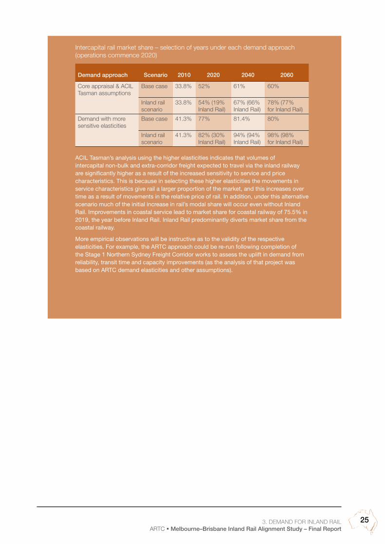
3. DEMAND FOR INLAND RAILARTC Melbourne–Brisbane Inland Rail Alignment Study – Final Report
25
Intercapital rail market share – selection of years under each demand approach (operations commence 2020)
Demand approach Scenario 2010 2020 2040 2060
Core appraisal & ACIL Tasman assumptions
Base case 33.8% 52% 61% 60%
Inland rail scenario
33.8% 54% (19% Inland Rail)
67% (66% Inland Rail)
78% (77% for Inland Rail)
Demand with more sensitive elasticities
Base case 41.3% 77% 81.4% 80%
Inland rail scenario
41.3% 82% (30% Inland Rail)
94% (94% Inland Rail)
98% (98% for Inland Rail)
ACIL Tasman’s analysis using the higher elasticities indicates that volumes of intercapital non-bulk and extra-corridor freight expected to travel via the inland railway are significantly higher as a result of the increased sensitivity to service and price characteristics. This is because in selecting these higher elasticities the movements in service characteristics give rail a larger proportion of the market, and this increases over time as a result of movements in the relative price of rail. In addition, under this alternative scenario much of the initial increase in rail’s modal share will occur even without Inland Rail. Improvements in coastal service lead to market share for coastal railway of 75.5% in 2019, the year before Inland Rail. Inland Rail predominantly diverts market share from the coastal railway.
More empirical observations will be instructive as to the validity of the respective elasticities. For example, the ARTC approach could be re-run following completion of the Stage 1 Northern Sydney Freight Corridor works to assess the uplift in demand from reliability, transit time and capacity improvements (as the analysis of that project was based on ARTC demand elasticities and other assumptions).

B. Route development and costing 4. Performance specification
and design standards
4. PERFORMANCE SPECIFICATION AND DESIGN STANDARDSARTC Melbourne–Brisbane Inland Rail Alignment Study – Final Report
26

4. PERFORMANCE SPECIFICATION AND DESIGN STANDARDSARTC Melbourne–Brisbane Inland Rail Alignment Study – Final Report
27
4. Performance specification and design standards
A range of performance specifications were developed for the inland railway to assist development of the route and costing of track and train operating costs.
As no inland route currently exists between Melbourne and Brisbane, there is an opportunity to develop new standards for both rollingstock and below rail infrastructure. These new standards are considered in terms of both the capital cost and operational benefits.
Building the inland railway to a higher standard would allow increased speeds and axle loads. However the higher standard would require additional capital expenditure. Building the railway to a lower standard would result in reduced capital costs at the expense of operational restrictions.
The proposed route uses a considerable amount of existing track in order to reduce capital cost. upgrading the entire route to a higher standard would be very expensive due to the long distances involved. Therefore operating the entire inland railway to a higher standard is not considered a viable initial option. Existing standards are adopted where existing track is used.
New sections of track could be constructed to a higher standard, a lower standard or to existing Class 1 standards. Class 1 standards have been developed and refined over years of operating freight railways in Australia; therefore constructing to a lower standard would not be efficient. Sections of new track could be constructed to:
A higher standard (not currently used in Australia) or
Current Class 1 standards.
4.1 Higher standard
The main benefit of a higher standard of track is increased line speed and axle loads. As a considerable amount of existing track would be used, axle loads would be restricted to the limits imposed by existing track. (Reorganising loads as trains progress along the route would not provide any significant operational benefits).
A higher track specification would allow trains to travel with a higher axle load at higher speeds over the new track sections. To operate at higher speeds, new rollingstock would be required as existing rollingstock is designed for existing Class 1 track standards. Additional capital expenditure would also be required to build the higher standard track because there is no proposal to increase maximum line speeds for freight trains on the ARTC network. The operator would be restricted to using the full potential of that rollingstock on the new, more highly specified parts of the inland route only.
4.2 Current Class 1 standards
Adopting current (or similar) standards for both existing and new track offers considerable benefits: rail operators could operate the same rollingstock as they currently do on the network; maintenance routines and techniques from the existing network could be applied on the inland route; and construction methods, materials and equipment would remain unchanged. Higher speed services (above 115 km/h) could still operate on the route, but they would be required to operate at a lower axle load.
For the above reasons, design standards have been developed for the inland railway that are consistent with the standards currently applying to other Australian railways. A combination of new track (constructed to Class 1C for increased speed and tonnage) and existing Class 1 and Class 2 track (current standards) would be adopted for the railway. Any existing Class 3 track would be upgraded to Class 1C to allow for higher axle loads than are currently permitted on Class 3 track.
4.3 Future proofing
New alignments will be designed for possible future higher speed operation by adopting large radius curves wherever possible. Although future upgrading of lines could involve the use of larger rail, heavier sleepers or deeper formations, it is recognised that the alignment itself is generally fixed in the long term.
It is reasonable to assume that as a result of a future rollingstock upgrade, higher freight operating speeds would be possible. The possible track structure requirements for such future operations cannot be predicted at this stage. It is also possible that such an operation may not be introduced within the life of the initial track structure. However because the new alignment design (the position of the track on the ground) has essentially an infinite life, it is designed with future train operations in mind. This involves adopting large radius curves where it is practical to do so without incurring unreasonably high additional capital expenditure. This is especially possible for greenfield sites in open country, with few constraints on alignment design.
In the case of bridge structures, which have very long service lives, it is reasonable to try to predict potential future loads as the incremental cost of building to higher standards is small compared with the cost of replacing or upgrading a bridge prior to the end of its service life. The importance of anticipating the requirements of future train operations is reflected in the current ARTC design standard for bridges (BDS 06) which calls up a rating of 300-LA from the Australian Bridge Design Code as a design requirement for new and upgraded bridges. Therefore new and upgraded bridges on the inland railway will allow for 32 tonnes axle load.

4. PERFORMANCE SPECIFICATION AND DESIGN STANDARDSARTC Melbourne–Brisbane Inland Rail Alignment Study – Final Report
28
4.4 Design and performance standards for the inland railway
With this methodology in mind a set of design standards were developed for the inland railway. Individual performance specifications are presented in the table below. Further detail is presented in Appendix C.
TABLE 12 Inland railway performance specifications
Attribute Performance
Requirements
Maximum freight train transit time (terminal-terminal including crossing loop delays)
Target driven by a range of customer preferences and less than 28 hours Melbourne-Brisbane
Inland rail route distance (Melbourne–Brisbane) Less than coastal route
Gauge Standard (1,435 mm) (with dual gauge in some Queensland sections)
Desirable max freight operating speed 115 km/h @ 21 tonnes axle load (lower axle load, passenger trains, if any, could be 130–160 km/h)
Maximum* axle loads 21 tonnes at 115 km/h (for containers) (higher axle load, e.g. 25 tonnes would be permitted at lower speeds, such as 80 km/h)
Reliability Not less than coastal route
Operating costs End-to-end, lower than coastal route
Minimum vertical clearance above top of rail (to allow for double stacking)
7.1 m for new structures, any amendment to existing structures to be dependent on economic benefit
ARTC’s forward plans provide for double stacking from Melbourne to Parkes (Sydney–Cootamundra in 2015 and Cootamundra–Melbourne in 2016) 21
Assumed maximum train length 1,800 m
Minimum Design Standards
Fast inland alignments Speed / Grade / Curvature
115 km/h / 1 in 100 / 800 m radius
Medium speed mountainous alignments Speed / Grade / Curvature
60–80 km/h / 1 in 50 / 400 m radius
Corridor width 40 m
Operational standards
Reference train (basis for operational standards)
Rolling stock is in service now, maximum speed of 115 km/h, double stacking of containers. Comprises:
Three 3,220 kW, AC drive, diesel electric locomotives, 22 m long, weighing 130 t each, and able to operate on 21 t axle load track. These are similar to the AC drive locomotives currently on interstate freight service
Seven five-pack bogie container well wagons, each 105m long, weighing 100t tare and capable of carrying 20 TEu double stacked. These are similar to RQZY or RRZY type wagons
Thirty-eight (38) bogie container flat wagons, each 25.75 m long, weighing 22 t tare and capable of carrying 4 TEu single stacked. These are similar to CQMY type wagons
* Can be increased in future with larger rail, heavier sleepers or deeper formation. New bridges, which have very long service lives, allow higher axle loads (32 tonnes), as the incremental cost of building to higher standards is small compared with the cost of replacing or upgrading a bridge prior to the end of its service life.
21 ARTC 2008, 2008-2024 Interstate and Hunter Valley Rail Infrastructure Strategy, 30 June 2008, p33

4. PERFORMANCE SPECIFICATION AND DESIGN STANDARDSARTC Melbourne–Brisbane Inland Rail Alignment Study – Final Report
29
4.5 Single track
A further important assumption about the inland railway is that it will be single track for most of its length. For the coastal railway from Junee to Melbourne, ARTC plans to duplicate this track around 2013.22
The box below provides information about single track railways.
22 ARTC 2008, 2008-2024 Interstate and Hunter Valley Rail Infrastructure Strategy, 30 June 2008, p33
BOX 6 Single track railway
Many railways in Australia and around the world are single track, where trains run in both directions on the one line. The extra cost of double track (providing separate tracks for each direction of travel) is only justified for busy lines with high volumes, particularly those used for commuter services in cities or on busy freight lines like the Hunter Valley.
On a single track railway, trains running in opposite directions can pass one another only where sections of track are provided for this purpose, termed passing loops or crossing loops. (In railway terminology, trains passing one another are said to ‘cross’.) The same applies to overtaking moves: for example a passenger train can only overtake a slower freight train at a loop, where the freight train waits for the faster train to go past. The term ‘passing lanes’ is sometimes used for longer loops, for example those which have been built on the remaining sections of single line between Melbourne and Sydney.
The process of crossing trains on a single track railway will always result in delays to at least one of the trains involved, as the train that enters the crossing loop must stop to wait for the opposing train to pass. The length of this ‘crossing delay’ will depend on the relative timing of the two trains’ arrival at the crossing loop. The challenge is to reduce crossing delays to a minimum, through the provision and optimum placement of adequate loops, and though timetabling and control of train operations, and through trains being driven within times allowed on each section. Modern signalling and control systems, such as ATMS (planned to be introduced by ARTC and assumed for the inland railway), assist in managing crossing movements. Nevertheless some level of delay due to crossings is inevitable, and must be allowed for in the timetable. In principle, delay on single track lines is minimised by a combination of adequate capacity, modern signalling and operational control, appropriate driving and use of reliable rollingstock. Thus all stakeholders are involved.
As traffic grows on a single track railway, the number of crosses experienced by each train increases and hence the total crossing delays increase – leading to a longer end-to-end journey time for each train. The most cost-effective way to reduce these delays is to build more crossing loops. If this is done, a train will not have to wait so long for an opposing train to arrive and go past, allowing it to resume its journey sooner, thus reducing the delay associated with each individual cross. Adding loops is usually a much more cost-effective way of reducing overall transit time than shortening the line by building new track, termed a deviation.
On the inland railway it has been assumed that sufficient crossing loops will be provided in the initial construction to cater for the level of traffic expected at that time and for some future traffic growth.
Train ATrain B
4.6 Track categories
The design, construction and maintenance of railways in Australia are documented in standards that generally cover individual states or apply network-wide. Different principles are adopted in the various locations, although a national code of practice is expected to be in place by the time the inland railway is in operation.
For the purposes of this report, the use of track categories (Class 1 and Class 2) has been adopted for the specification of standards for the construction and maintenance of the proposed and existing alignments.

5. The route
5. THE ROuTEARTC Melbourne–Brisbane Inland Rail Alignment Study – Final Report
30

5. THE ROuTEARTC Melbourne–Brisbane Inland Rail Alignment Study – Final Report
31
5. The routeThis chapter presents the analysis undertaken throughout the study to determine the optimum route from Melbourne to Brisbane within the far western sub-corridor. The approach to route analysis was to initially consider broad route options, then to progress through to more detailed refinement of the alignment. The study adopted a process in which the options were analysed in stages; in terms of operational, engineering and environmental factors. At each stage the options were analysed in sufficient detail to enable key decisions to be made and finally narrow the options down to a single alignment. The successive stages of route analysis included:
Inland Rail route options – identification of a range of available route options
Identification of the route – evaluation of the route options and preliminary analysis for the following areas: Melbourne to Parkes; Parkes to Moree; and Moree to Brisbane
Analysis of the route – the route was analysed in terms of capital cost, environmental impacts and journey time as well as its preliminary economic and financial viability
Development of the alignment – the alignment was developed considering environmental and engineering factors.
Appendix D presents the options within the far western corridor. Appendix E contains a rigorous analysis aimed at identifying a single alignment for the inland railway. The final alignment is presented in Appendix F – Maps of the proposed alignment.
5.1 Inland Rail route options
The objective of the options review was to identify the available route options between Melbourne and Brisbane, commencing at South Dynon and ending at Acacia Ridge. The options were analysed to:
understand the technical features of each route and provide the necessary supporting information
Provide initial environmental assessment, capital cost and journey time estimates for the inland route
Identify engineering data, environmental constraints and operational measures relevant to the route options under consideration.
A map showing the main route options for the inland railway is provided at Figure 11 on page 32.
5.2 Identification of the route
The characteristics and details of numerous route options and sections provide a plethora of possible alternatives for the overall route between Melbourne and Brisbane. In all, there were over 50,000 possibilities. Because it was not feasible to analyse each of them, the following key criteria were adopted for the purpose of preliminary route selection:
Capital cost
Journey time.
These criteria were used to establish a shortlist of route options which were subjected to more detailed technical, financial and economic assessment.
Journey time versus capital cost analysis
The overall route was divided into three areas: Melbourne to Parkes; Parkes to Moree; and Moree to Brisbane. Each of these areas was analysed to identify the routes that would present the best value (considering journey time and cost).
After all options were included on a graph of indicative journey time against capital cost, an ‘efficiency frontier’ was identified for each area. This involved identifying the set of options with the lowest capital cost for any given journey time. This set then comprised those options worthy of further consideration. Other combinations had higher costs and/or journey times, so were not further considered.
This analysis is illustrated in Figure 10 below.
FIGuRE 10 Analysis of options in each area
After indentifying the best value options in each area, it was possible to select various routes between Melbourne to Brisbane based on any combination of the routes identified between Melbourne and Parkes, Parkes and Moree and Moree and Brisbane. These combinations were graphed in the same way as each area: with the boundary of efficiency identified (and shown in grey at Figure 10), sub-optimal options were eliminated.
Options not due for further condiserationOptions to be taken forwardBoundary of efficiency
Incr
easi
ng c
apita
l co
st
Increasing journey time

5. THE ROuTEARTC Melbourne–Brisbane Inland Rail Alignment Study – Final Report
32
FIGuRE 11 The main route options for the inland railway
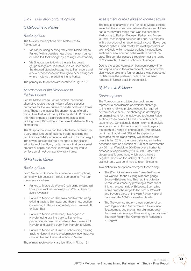
5. THE ROuTEARTC Melbourne–Brisbane Inland Rail Alignment Study – Final Report
33
5.2.1 Evaluation of route options
(i) Melbourne to Parkes
Route options
The two key route options from Melbourne to Parkes were:
Via Albury, using existing track from Melbourne to Parkes (with a possible new direct line from Junee or Illabo to Stockinbingal by-passing Cootamundra)
Via Shepparton, following the existing broad gauge Mangalore–Tocumwal line via Shepparton, the disused standard gauge line to Narrandera and a new direct connection through to near Caragabal where it rejoins the existing line to Parkes.
The primary route options are identified in Figure 12.
Assessment of the Melbourne to Parkes section
For the Melbourne to Parkes section the various alternative routes through Albury offered superior outcomes for the key criteria of capital costs and transit time. Though the fastest Shepparton route offered a transit time that would be quicker by about 30 minutes, this route attracted a significant extra capital cost (adding over $900 million to the project relative to Albury alternatives).
The Shepparton route had the potential to capture only a very small amount of regional freight, reflecting the dominance of Melbourne as a destination for that freight. The advantages of this route fell short of the sizable advantage of the Albury route, namely, that only a small amount of capital expenditure would be required to achieve an almost comparable transit time.
(ii) Parkes to Moree
Route options
From Moree to Brisbane there were four main options, some of which possess multiple sub options. The four routes are as follows:
Parkes to Moree via Werris Creek using existing rail lines (new track at Binnaway and Werris Creek to avoid reversals)
Parkes to Moree via Binnaway and Narrabri using existing track to Binnaway and then a new section connecting to the existing railway near Emerald Hill or Baan Baa
Parkes to Moree via Curban, Gwabegar and Narrabri using existing track to Narromine, predominately new track between Narromine and Narrabri and existing track from Narrabri to Moree
Parkes to Moree via Burren Junction using existing track to Narromine and predominately new track via Coonamble and Burren Junction to Moree.
The primary route options are identified in Figure 13.
Assessment of the Parkes to Moree section
The results of analysis of the Parkes to Moree options were that the journey time between Parkes and Moree had a much wider range than was the case from Melbourne to Parkes. Between Parkes and Moree, journey times ranged between 341 and 724 minutes with a corresponding range in capital cost. Slower but cheaper options used mostly the existing corridor via Werris Creek while the faster options included large sections of new corridor in the western part of the area. This corridor passed through or near the towns of Coonamble, Burren Junction or Gwabegar.
Due to the strong correlation between journey time and capital cost in this area none of the options was clearly preferable; and further analysis was conducted to determine the preferred route. This has been reported in further detail in Appendix E.
(iii) Moree to Brisbane
Routes options
The Toowoomba and Little Liverpool ranges represent a considerable operational challenge to the inland railway project meeting its required performance criteria. The challenge in developing an optimal route for the Inglewood to Acacia Ridge section was to balance transit time with capital expenditure. Considerable design work and analysis was performed in this region which went beyond the depth of a range of prior studies. This analysis confirmed that almost 50% of the capital cost estimated for an inland railway would be incurred over this last 26% of the route distance, as the line descends from an elevation of 690 m at Toowoomba or 450 m at Warwick to 60–80 m over a horizontal distance of approximately 20–30 km. Rather than stopping at Toowoomba, which would have a negative impact on the viability of the line, the optimal route was confirmed to reach Brisbane.
Two distinct route options emerged, these being:
The Warwick route – a new ‘greenfield’ route via Warwick to the existing standard gauge Sydney–Brisbane line. This had the potential to reduce distance by providing a more direct link to the south side of Brisbane. Such a line would cross the range to the east of Warwick and traverse parts of the Main Range National Park near the NSW/Queensland border
The Toowoomba route – a new corridor direct from Inglewood to Millmerran and Oakey, near Toowoomba, and then a new alignment down the Toowoomba range; thence using the proposed Southern Freight Rail Corridor from Rosewood to Kagaru.

5. THE ROuTEARTC Melbourne–Brisbane Inland Rail Alignment Study – Final Report
34
FIGuRE 12 Albury and Shepparton route options schematic

5. THE ROuTEARTC Melbourne–Brisbane Inland Rail Alignment Study – Final Report
35
FIGuRE 13 Parkes to Moree route options schematic

5. THE ROuTEARTC Melbourne–Brisbane Inland Rail Alignment Study – Final Report
36
The primary route options to reach Brisbane are identified in Figure 14.
Assessment of the Moree to Brisbane area
The results of the analysis indicated that the route via Toowoomba had stronger economic merit. Although the Warwick routes were faster than the Toowoomba options, they were also significantly more expensive. Although approximately 20 minutes would be saved, this would be at a cost of almost $450 million.
FIGuRE 14 Toowoomba and Warwick route options schematic

5. THE ROuTEARTC Melbourne–Brisbane Inland Rail Alignment Study – Final Report
37
The Toowoomba option had the added benefit of capturing additional regional freight (mainly coal) compared to the Warwick option.
5.2.2 Determination of an end-to-end route
Results
The cost-effective routes from each of the three areas were combined to analyse the overall route between Melbourne and Brisbane.
Considering the different segments of journey time, key findings from the analysis shown in Figure 15 below were as follows:
Between transit times of 28 and 20 hours, substantial gains were achieved by pursuing faster options in the Parkes to Moree area. These were, first, upgrading the existing track, then constructing a deviation between Premer and Emerald Hill, then constructing a new route via Gwabegar or Coonamble. These options all travelled via Albury and Toowoomba
In this same journey time range, the smaller steps included the option of adding a direct link from Junee/Illabo to Stockinbingal
More expensive options were required to achieve a significantly faster transit time. These involve, first, moving to a Warwick route, then the route via Shepparton, then both.
Route for further analysis
The efficiency frontier, shown in red at Figure 15, indicates that increasingly high capital costs are required to achieve the shortest journey times. The most expensive options were therefore not analysed further – in particular, no options via Warwick or Shepparton were considered further. There was not a sufficient demand change nor a sufficient impact on economic viability (brought about by a 45 minute reduction in the journey time) to justify additional capital expenditure of around $1 billion. If such a reduction in transit time was identified as significant, it could be achieved in a more cost effective manner by adding crossing loops to reduce crossing delays, rather than adopting a more expensive route via Warwick. In any event demand on the route via Warwick would have been lower because it would not have carried coal from Toowoomba to Brisbane.
FIGuRE 15 Melbourne to Brisbane route options
29.0024.00 28.0023.00 27.0022.00 26.0021.00 25.0020.00
6
5
4
3
0
8
Cap
ital c
ost
($ b
illio
n)
Journey time – including crossing delays (hours)
Via Temora Junction
Via Cootamundra
Direct line from Junee to Stockinbingal Options via Werris Creek
(no upgrade)
Options via Werris Creek (upgraded)
Options via Premer–Emerald Hill
Options via Coonamble
Options via Warwick and Albury
Options via Toowoomba and Shepparton
Options via Warwick and Shepparton
Boundary of efficiency
Options via Toowoomba and Albury

5. THE ROuTEARTC Melbourne–Brisbane Inland Rail Alignment Study – Final Report
38
FIGuRE 16 Short-listed inland railway routes for analysis

5. THE ROuTEARTC Melbourne–Brisbane Inland Rail Alignment Study – Final Report
39
The short-listed routes identified as requiring further analysis are depicted in Figure 16.
5.3 Analysis of the short-listed routes
The short-listed routes identified for analysis comprised generally existing track from Melbourne to Parkes via Albury, and then from Parkes to Narromine. Between Narromine and Narrabri the two route options were via the existing track towards Werris Creek or greenfield construction via (or near) Gwabegar. Existing corridors would be used between Narrabri and North Star, greenfield railway (using existing narrow gauge corridors where available) to Inglewood, Millmerran, Gowrie, Grandchester/Rosewood and Kagaru. The last section from Kagaru to Acacia Ridge would use existing standard gauge track. Within the study area for these route options opportunities exist to improve the journey time by upgrading existing track or constructing deviations.
The option using the existing track towards Werris Creek was chosen to represent the lowest capital expenditure option meeting the performances specification and had an approximate length of 1,880 km.
The option using the more direct route between Narromine and Narrabri was chosen to represent the fastest transit time for a reasonable capital expenditure and had an approximate distance of 1,731 km.
5.3.1 Evaluation of deviations
A number of potential options were differentiated based on capital cost and journey time. The options with the lowest capital cost per minute saved were considered the most cost effective options. Analysis showed many of the options to be less favourable because of:
Negative environmental impacts and land use constraints
Significant capital expenditure
The upgrading of track did not give significant journey time improvement (due to curves and grades still constraining the speed of the train)
Options to remove speed constraints were costly for little time saving.
Based on this analysis the following options were identified for further alignment development.
Common to both routes
Illabo to Stockinbingal – as it shortened the route
upgrade from Class 2 to Class 1 from Parkes to Narromine and Narrabri to Moree – as it reduced transit time by increasing maximum speed
Camurra deviation – as it shortened the route
North Star to Yelarbon – as there was a higher cost associated with the alternative via Kildonan
Oakey bypass – because it required less capital expenditure than upgrading the track through Oakey.
Towards Werris Creek
Narromine bypass – as it shortened the route
Dubbo bypass – as it avoided the replacement of the existing Macquarie River bridge
Merrygoen deviation – as it shortened the route
Piambra to ulinda deviation – as it shortened the route
Spring Ridge to Breeza – as it shortened the route
Narrabri bypass (east) – as it avoided bridge replacement on the existing railway.
Via Narromine to Narrabri
Narromine to Curban – as it was more cost effective than an upgraded route via Dubbo
Curban to Gwabegar – as it required less capital expenditure than the upgrade from Curban to Coonamble and new track from Coonamble to Gwabegar

5. THE ROuTEARTC Melbourne–Brisbane Inland Rail Alignment Study – Final Report
40
Narrabri bypass (west) – because of the significant speed constraints in Narrabri and the cost of upgrading the existing bridge and track.
5.3.2 Comparison of the routes
Capital cost and journey time
Having confirmed the deviations to be included, preliminary capital cost, operational cost and transit time estimates were developed to compare the two short-listed routes. They were used as inputs to economic and financial analysis undertaken earlier in the study.
The results of the analysis were:
The 1,731 km route offered a journey time approximately 6 hours less than the 1,880 km route, which resulted in reduced operational costs
The 1,880 km route required about 30% less capital expenditure than the 1,731 km route.
Demand
Key findings of the preliminary demand analysis undertaken for the 1,880 km and 1,731 km options were as follows:
The 1,731 km scenario was estimated to result in higher demand levels for Melbourne–Brisbane intercapital freight. However, total tonnage on the shorter route was lower than the 1,880 km route because the shorter route did not capture coal from the Gunnedah basin
Inland Rail’s share of total road and rail intercapital freight was estimated as being higher for the 1,731 km route.
Financial and economic analysis
Preliminary economic and financial appraisals were undertaken to compare the 1,880 km and 1,731 km inland railway scenarios.
These analyses found that:
Financial viability of the project worsened under the 1,731 km scenario. Although intercapital access revenue increased slightly, revenue from the transport of Gunnedah basin coal was lost and capital costs were higher
Inland Rail did not achieve a positive economic NPV at a 7% discount rate, but the 1,731 km scenario made Inland Rail’s economic result less negative than the 1,880 km scenario due mainly to operational cost savings.
In summary, the 1,731 km scenario improved Inland Rail’s economic result but not its financial result.
Route for development
Compared with the 1,880 km route, the 1,731 km route had superior economic results. Although the 1,880 km route had a better financial result, neither scenario was financially viable. Therefore the focus for more detailed route, demand, economic and financial analysis moved to the 1,731 km option incorporating the direct route from Narromine to Narrabri.
5.4 Developing the final alignment
5.4.1 Refining the alignment
The refinement of the proposed inland railway alignment incorporated an iterative process with evaluation of the following factors:
Environmental and land issues
Railway operations considerations
Engineering assessments
Capital cost estimates.
The culmination of the refinement process was to reduce the alignment options to a single alignment.
5.4.2 Track duplication or dual gauge
In Queensland the existing railway has narrow gauge tracks. To provide a standard gauge track for the inland railway, either a dual gauge or a railway comprising separate standard and narrow gauge tracks would be required. Preliminary cost estimates showed that upgrading to dual gauge along existing alignments would generally be more cost effective than providing additional standard gauge tracks adjacent to the existing narrow gauge railway; and would involve less environmental/land use impacts. Double-track narrow-gauge corridors would be replaced by double-track dual-gauge. Figure 17 shows where standard gauge or dual gauge has been assumed.

5. THE ROuTEARTC Melbourne–Brisbane Inland Rail Alignment Study – Final Report
41
5.4.3 The route approaching Brisbane
In recent studies, Queensland Government agencies have developed alignments in the corridor from Toowoomba to Brisbane, which were reviewed in the course of developing a proposed alignment for the inland railway. The two specific areas are between Gowrie and Grandchester and between Rosewood and Kagaru.
In developing an alignment for the inland railway, the study team worked closely with the Queensland Government in order to identify the best option in this area. Different solutions have been adopted for each of these sections.
Between Rosewood and Kagaru, the Queensland Department of Transport and Main Roads (TMR) has been conducting a separate study, somewhat in parallel with this study, known as the Southern Freight Rail Corridor (SFRC) Study. TMR’s study has included extensive public consultation and engagement with affected parties. The parameters for the SFRC have been developed with freight trains in mind. Whilst not identical to that used for the inland railway (for example, a maximum train length of 2 km was allowed for, as against the 1,800 m used in this study), the general arrangement of the SFRC is close enough that the route identified by TMR has been adopted for the inland railway and included in the scope of works required.
FIGuRE 17 Standard and dual gauge corridors
Between Gowrie and Grandchester, the route initially developed by (the then) Queensland Transport and finalised in 2003, was designed with the aim of providing for future higher speed passenger services as well as freight west from Brisbane. Accordingly, the alignment catered for speeds up to 200 km/h and to achieve this included two tunnels, long and high viaducts and extensive earthworks. This alignment has been preserved in local government planning schemes. After analysing this alignment alongside other options, this study concluded that the previous Gowrie to Grandchester alignment was not the optimum solution for the inland railway. This study found that the journey time savings from a superior alignment in this area were more expensive than could be obtained by improving the alignment of other sections of the inland railway. In addition, freight train speeds through this area are more likely to be dictated by train performance, particularly westbound trains up the steep grade, rather than the track curvature. This study also had reservations about the feasibility of operating long, slower freight trains on the same corridor as fast passenger trains. Accordingly, an alternative route was identified for the inland railway between Gowrie and Grandchester, with specifications more appropriate to operation of intercapital freight trains.

5. THE ROuTEARTC Melbourne–Brisbane Inland Rail Alignment Study – Final Report
42
5.4.4 Summary of proposed alignment
The proposed inland railway comprises a 1,731 km long alignment between South Dynon in Melbourne and Acacia Ridge in Brisbane:
Melbourne to Parkes – 670 km of existing Class 1 track and 37 km of greenfield track from Illabo to Stockinbingal bypassing Cootamundra and the Bethungra spiral
Parkes to North Star – 307 km of upgraded track and 291 km of greenfield alignment from Narromine to Narrabri
North Star to Acacia Ridge – 271 km of greenfield construction, 119 km of existing track upgraded from narrow gauge to dual gauge and 36 km of the existing coastal route.
TABLE 13 Proposed track types
Track type Length (km) Percentage (%)
Existing track 706 41
upgraded track 307 18
upgraded narrow gauge 119 7
New track 599 34
Total 1,731 100
The proposed route is presented in Figure 18. More detailed maps are presented in Appendix F – Maps of the proposed alignment.

5. THE ROuTEARTC Melbourne–Brisbane Inland Rail Alignment Study – Final Report
43
FIGuRE 18 Proposed Inland Rail route

6. Environment and planning
6. ENVIRONMENT AND PLANNINGARTC Melbourne–Brisbane Inland Rail Alignment Study – Final Report
44

6. ENVIRONMENT AND PLANNINGARTC Melbourne–Brisbane Inland Rail Alignment Study – Final Report
45
6. Environment and planningA Preliminary Environmental Assessment (PEA) and a Legislation Review and Planning Approvals Strategy were prepared, and are summarised in this chapter. The assessment and strategy are discussed in Appendix H and I respectively.
6.1 Preliminary Environmental Assessment
The purpose of the PEA was to:
Identify the key environmental risks for each route section of the proposed alignment
Identify potential mitigation measures
Outline likely future assessment requirements.
6.1.1 Development of the proposed alignment
After consideration of broad and local alignment alternatives, the proposed alignment was developed and refined. The aim in doing so was to avoid major environmental and land use constraints and to integrate ecologically sustainable development principles into the design of the alignment. Where possible, the alignment was shifted to minimise impacts on, for example, protection areas, significant tracts of vegetation and residences.
6.1.2 Environmental risk assessment
An environmental risk assessment was undertaken for each route section taking into consideration the environmental constraints and the works proposed. Environmental issues identified were assigned a risk category of A, B or C through a workshopping process (refer to Section 2.2 of Appendix H for descriptions of these risk categories and environmental risk assessment data sheets for each route section of the proposed alignment).
Environmental issues in category A were considered to be more significant risks and these received greater attention during the Preliminary Environmental Assessment. Table 14 summarises the environmental issues that were given a risk category of A.
6.1.3 Environmental assessment methodology
A desktop assessment of environmental impacts was undertaken for the proposed route. This desktop assessment reviewed aerial photography and spatial information that had been collected and loaded into a Geographic Information System (GIS) database. Searches of the Environment Protection and Biodiversity Conservation Act 1999 (EPBC Act)23 and other relevant databases were also undertaken for each of the greenfield alignments.
The spatial information reviewed included, but was not limited to, threatened species data, vegetation mapping, administrative boundaries of protection areas (such as State Forests, National Parks and State Conservation Areas), records of previously recorded Indigenous sites and items, listed non-Indigenous sites/items and hydrological information such as the locations of drainage lines, watercourses and designated flood areas.
6.1.4 Key environmental impacts
Flora and fauna
Some of the most significant environmental impacts of the project were those associated with vegetation removal required for construction of the railway. Impacts associated with the removal of vegetation included effects on threatened species, populations and ecological communities, the fragmentation of wildlife areas and habitats, and severance of wildlife corridors.
23 Protected matters search tool.
TABLE 14 Summary of environmental issues with risk category A
Route section Environmental issues with risk category of A
Curban to Gwabegar Protection areas; flora and fauna
Gwabegar to Narrabri Protection areas; flora and fauna
Narrabri bypass Hydrology and flooding
North Star to Yelarbon Flora and fauna
Inglewood to Millmerran Protection areas; flora and fauna
Gowrie to Helidon Flora and fauna
Grandchester to Kagaru Flora and fauna

6. ENVIRONMENT AND PLANNINGARTC Melbourne–Brisbane Inland Rail Alignment Study – Final Report
46
Protection areas
Construction of the inland railway would affect protection areas on sections of the route between Curban and Narrabri, and from Inglewood to Millmerran, where the proposed alignment crosses areas of state forest. These areas of land, and the severed parcels of state forest, would have to be acquired or swapped. The designation of the land as state forest would need to be revoked (which would require an Act of Parliament) in order to allow the development of the railway. Consultation would have to be carried out with the appropriate NSW and Queensland government agencies during the concept design development.
Hydrology and flooding
Potential hydrological impacts, such as flooding, channelling, flow redirection and erosion occur where the proposed alignment crosses floodplains or significant watercourses. The proposed alignment crosses designated flooding areas on the Narromine to Curban, Curban to Gwabegar, Narrabri bypass and Camurra deviation route sections. The proposed alignment crosses significant watercourses on the Gwabegar to Narrabri, North Star to Yelarbon and Grandchester/Rosewood to Kagaru route sections.
Indigenous heritage
Indigenous archaeological items/sites, and places of Indigenous cultural significance could be affected by construction of the proposed alignment. The Preliminary Environmental Assessment was limited to consideration of previously recorded Indigenous sites only. Numerous previously recorded Indigenous items/sites exist within the vicinity of the proposed alignment. The proposed alignment avoids these sites. However given the presence of previously recorded sites along these routes, there is great potential for unrecorded sites to exist in these areas.
Noise
Adverse noise impacts may occur during construction of the proposed railway. These impacts would be most severe in built up areas. Standard construction noise mitigation measures would be implemented as part of the overall construction environmental management plan (CEMP) for the project.
During the operation of the project, potential adverse noise impacts would occur to residences within the vicinity of the alignment. Increased levels of noise could arise from either the introduction of rail traffic into an area or rail traffic increasing as a result of the project. Detailed noise impact assessments would have to be carried out to determine the level of impact along the alignment. Where train operations lead to noise criteria being exceeded, noise mitigation measures would need to be developed and implemented. Mitigation measures could include acquisition of properties, installation of noise walls or architectural treatment.
6.2 Planning approvals strategy
6.2.1 Overview
A review of all relevant Commonwealth, state and local legislation was undertaken to identify the likely statutory approvals required for the project and provide an overarching approvals framework for the project. From this review and based on the findings of the PEA, key planning and land use issues were considered and high-level strategies have been identified to achieve the efficient and timely delivery of the project. The key legislative processes and a framework for planning approval is provided in Appendix I and summarised below.
6.2.2 Approvals delivery framework
The inland railway project would trigger approvals under Commonwealth, NSW and Queensland legislation. No approvals under Victorian legislation would be required. Figure 19 provides an overview of the recommended approvals process for the project.

6. ENVIRONMENT AND PLANNINGARTC Melbourne–Brisbane Inland Rail Alignment Study – Final Report
47
Secondary Approvals (various Qld legislation)
Primary approvals under federal and state legislation
The Commonwealth EPBC Act requires a project proponent to refer a project to the Commonwealth Minister for the Environment, Water, Heritage and the Arts for determination as a ‘controlled action’. If declared a controlled action, the project would require assessment under the Environment Protection and Biodiversity Conservation Act 1999 and approval from the Commonwealth minister before it could proceed. However, the minister can approve the project through the respective state assessment processes under the Commonwealth/state bilateral agreement.
Given the scale of the project and the natural and cultural environments through which it would pass, it is highly likely the project would be considered a controlled action.
In NSW the project would be assessed as a ‘major project’ in accordance with the provisions of Part 3A of the Environmental Planning and Assessment Act 1979 (EP&A Act). A ‘Concept Approval’ under Part 3A of the EP&A Act would initially provide a degree of certainty about the project’s overall viability without having to commit up-front to costly and time-consuming detailed design and assessment of the project. Subsequent approvals could then be staged, either as ‘Project Approval’ under Part 3A of the NSW EP&A Act, or through self-determination under Part 5 of the Act where effects are not deemed to be significant.
In Queensland the project would most likely be declared a ‘significant project’ and assessed through an Environmental Impact Statement (EIS) under the State Development and Public Works Organisation Act 1971 (SDPWO Act). Because of the overall length of new rail corridor, it is unlikely that the project would be assessed in one package. However under the Queensland SDPWO Act the project can be broken down into discrete components and staged according to an overall delivery strategy.
Following approval under the ‘primary’ state approvals, it is likely that the project would also require additional approvals from a number of different state and local agencies.
Timeframes
Based on typical timeframes for approvals processes for other large linear infrastructure projects, between 12 and 24 months would be required for completion of an EIS/Part 3A Environmental Assessment, and up to 12 months to secure additional approvals under other legislation and regulations. Revocation of state forest dedicated land, as required in both NSW and Queensland, would also have a significant bearing on the project delivery program owing to the requirement for lengthy negotiations and ultimately parliamentary approval.
Commonwealth
Environment Protection and Biodiversity Conservation Act
1999 (EPBC Act)
Referral under EPBC Act of Project to the
Minister for determination as Controlled Action
If a Controlled Action –Assessment under the
provisions of the EPBC Act
State process
NSW Environmental Planning & Assessment Act 1979
(EP and A Act)
Qld State Development and Public Works Organisation Act
1971 (SDPWO Act)
Assessed as ‘Major Project’ through Concept Plan Approval
under Part 3A of the EP and A Act
Assessd as ‘Signicant Project’ through EIS process under
s26 of SDPWO Act
Secondary Approvals (various NSW legislation)
Project Approval under Part 3A of the EP and A Act
Approval under Part 5 of the EP and A Act
Bila
tera
l Agr
eem
ent
FIGuRE 19 Approvals delivery framework

6. ENVIRONMENT AND PLANNINGARTC Melbourne–Brisbane Inland Rail Alignment Study – Final Report
48
6.2.3 Key strategies
Five high-level strategies have been identified to address the key risks and considerations for delivering the statutory approvals required for the project. The strategies provide a holistic approach to the planning and approval pathways for the project and encourage the efficient, transparent and collaborative approach to managing the multi-jurisdictional environmental planning approvals process of the project. These strategies include:
Consultation with key stakeholders –Early engagement with community, government and political stakeholders to discuss project challenges from a multi-jurisdictional perspective; identifying potential hold-points in the planning approval process; documenting how and when stakeholder input into the defined environmental planning approvals pathway will occur
Environmental approvals steering committee – Setting up a steering committee to align, manage and co-ordinate the approvals process across jurisdictions, noting the assessment criteria and timeframes that are relevant to the project; facilitating efficient and effective communication between local, state and Commonwealth agencies
Approvals delivery framework approach – Preparing an overall delivery framework that would provide a high-level guidance to gaining approvals across jurisdictions in parallel with achieving compliance with state and Commonwealth legislation
Confirmation of specified timeframes –Confirming and documenting regulatory timeframes in the approvals delivery framework. The steering committee would identify and manage key planning approval hold-points including potential time delays and ‘stop the clock’ provisions
Appoint a dedicated project manager and state planning co-ordinators – Assigning senior dedicated personnel to these key roles to drive the approvals process on a day to day basis, within each jurisdiction’s nominated approvals pathway. The project manager would report to the steering committee to manage timing and additional approvals as required.
6.3 Corridor reservation
If the inland railway project is not committed for 10–20 years, future development along or adjacent to the inland railway alignment may compromise viability of the route by increasing costs associated with land acquisition or compensation, affecting the operations of the railway (e.g. safety, journey time, etc) or require amendments to the route.
Consideration should be given to taking steps to reserve the inland railway alignment under the relevant state legislation (as described in section 6.2.2 and Appendix I) to ensure that future development or land zoning does not compromise the corridor and ultimately the viability of the project.
Initially this would include consultation with the relevant state planning authorities (e.g. NSW Department of Planning and the Queensland Department for Infrastructure and Planning) to determine the preferred mechanism for corridor preservation. Subject to these discussions, the most likely strategies would include:
Within NSW the corridor be included on the State Environmental Planning Policy (Infrastructure) 2007 as an ‘interim rail corridor’ to ensure that the proponent is aware of any future development applications within or adjacent to the railway corridor
Within Queensland further environmental assessment be undertaken to enable the corridor to be reserved as a strategic rail corridor under the Sustainable Planning Act 2009 Community Infrastructure Designation.

6. ENVIRONMENT AND PLANNINGARTC Melbourne–Brisbane Inland Rail Alignment Study – Final Report
49

7. Delivery program and capital cost
7. DELIVERY PROGRAM AND CAPITAL COSTARTC Melbourne–Brisbane Inland Rail Alignment Study – Final Report
50

7. DELIVERY PROGRAM AND CAPITAL COSTARTC Melbourne–Brisbane Inland Rail Alignment Study – Final Report
51
7. Delivery program and capital costThe proposed inland railway involves considerable construction work between Illabo near Junee and Kagaru near Brisbane. This chapter presents the options for staging the works, the construction delivery program and the capital cost estimate. A detailed report is provided at Appendix J.
7.1 Staging options
7.1.1 Overview
The two major areas of construction for the inland railway are the standard gauge connection from North Star to Brisbane and the construction of a direct link between Narromine and Narrabri. Possible options for staging construction of the railway included:
Initially operating the railway using the existing railway via Werris Creek and deferring the construction of the direct link from Narromine to Narrabri
Deferring the construction of the Class 2 to Class 1 upgrades (from Parkes to Narromine and Narrabri to Moree) and the Illabo to Stockinbingal deviation with initial operation involving continued use of the existing railway via Cootamundra
Terminating the railway at Toowoomba and deferring the capital cost of the expensive mountainous alignments (with tunnels) from Toowoomba to Brisbane.
7.1.2 Operation via Werris Creek
This staging option involved initial construction of the route between North Star and Brisbane to complete the journey from Melbourne to Brisbane. Queensland coal traffic would still be captured in this initial operation scenario, and Melbourne to Brisbane traffic would use the existing railway via Werris Creek until the Narromine to Narrabri link was completed. The route via Werris Creek is longer and slower than the route that has been proposed.
The benefits of this route were tested in the comparison of a 1,731 km route (involving greenfield construction towards Gwabegar) and a 1,880 km route (via existing track towards Werris Creek) during analysis of route options. The outcomes of this analysis showed that the 1,880 km route resulted in more negative economic outcomes (with a lower BCR) than the proposed inland route. It was therefore not considered a beneficial staging option.
7.1.3 Staging of upgrades and Illabo to Stockinbingal deviation
This staging option involved construction of the connection from North Star through to Brisbane and the direct link between Narromine and Narrabri. The staged works would be the upgrades from Class 2 to Class 1 (from Parkes to Narromine and Narrabri to Moree) and the deviation from Illabo to Stockinbingal.
These deferred works would not fundamentally change the operation of the inland railway. They would be constructed during operation of the railway to allow the overall journey time to be maintained (as the traffic volumes grow and the crossing delays increase). The railway’s performance would not be compromised because of the staging of these works.
7.1.4 Toowoomba termination
This option involved construction of the railway from Melbourne to Toowoomba, and completing the remaining Toowoomba to Brisbane section at a later date. This would defer a significant proportion of the initial capital cost because of the high cost of crossing the Toowoomba Range. under this option there would be a longer pick up and delivery time by road from Toowoomba to Brisbane (approximately 125 km, or 2–3 hours).
Terminating the inland railway at Toowoomba resulted in a negative impact on estimated coal freight demand and a halving of the expected intercapital tonnage. This resulted in a 60% decrease in below rail revenue. under this option the economic BCR decreased by around 80% relative to the full Melbourne-Brisbane scenario, indicating lower efficiency of expenditure.
7.1.5 Outcome
Initial operation using the existing track via Werris Creek or terminating at Toowoomba reduced expected traffic volumes because of the inferior service offered. The benefit of deferred capital expenditure did not outweigh the disbenefit of the reduction in traffic.
On the other hand, deferring the Class 2 to Class 1 upgrades and the Illabo to Stockinbingal deviation does not compromise performance. Therefore these works could be deferred until traffic volumes increase. The deferred spending on these works was factored into the economic appraisal of the 2020 and 2030 scenarios for commencement of services on the inland railway. It was assumed that if Inland Rail commences operation in 2040, traffic volumes demanding the route at that time would be to a scale to warrant the full capital program being completed upfront in the initial 5-year construction period.

7. DELIVERY PROGRAM AND CAPITAL COSTARTC Melbourne–Brisbane Inland Rail Alignment Study – Final Report
52
7.2 Delivery program
The proposed Inland Rail route covers remote areas of central NSW and south-east Queensland and traverses differing terrain types from flood plains to mountainous areas (with tunnels). To improve construction efficiency, the works would be separated into discrete packages. This break up affects both the delivery cost and the delivery program.
The important features of the delivery program are:
The planning and approval process including preliminary design, approvals, tender and award period, land acquisition, etc. will add a significant period of time to delivery of the project. A period of 36 months for these activities has been assumed, but this may be exceeded for more complex sections
Pre-construction planning and approvals would need to be prioritised so that construction of sections on the critical path can commence as
early as possible. Sections with less complicated approvals could commence early to smooth project cash flow and ease demand for construction resources
Construction for initial operation is assumed to be undertaken over a five year period
The Toowoomba tunnel between Gowrie and Helidon is the longest single construction task with a duration closely approaching five years. It therefore warrants priority during the planning and approval process and will need to be managed effectively to allow the tunnel spoil to be used efficiently as fill for embankment construction.
The delivery program is set out in Figure 20. Sections adjacent to each other have been programmed in a way to allow continuation of work, minimal disruption in resource usage and to minimise establishment costs. The staged improvements have been shown for construction at a later date.
FIGuRE 20 Overall delivery program
Section of routeYear
Construction period Deferred works
-3 to 0 1 2 3 4 5 X X+1 Y Y+1 Z Z+1 Z+2
Pre-construction activities
Narromine – Curban
Curban – Gwabegar
Gwabegar – Narrabi
Narrabi West – Narrabi North
Camurra – North Star
North Star – Yelarbon
Yelarbon – Inglewood
Inglewood – Milmerran
Milmerran – Brookstead
Brookstead – Yargullen
Yargullen – Oakey
Oakey – Gowrie
Gowrie – Helidon
Helidon – Grandchester
Grandchester – Kagaru
Parkes to Narromine (upgrade)
Narromine to Camurra (upgrade)
Illabo to Stockinbingal
Note: X, Y and Z represent various years after operations commence on the inland railway. The timing of these years is dependent upon freight volumes.

7. DELIVERY PROGRAM AND CAPITAL COSTARTC Melbourne–Brisbane Inland Rail Alignment Study – Final Report
53
7.3 Capital cost estimate
7.3.1 Capital cost model
To develop the capital cost for the entire route, a model was developed to calculate the cost for each package of work.
The capital cost model was split into three categories: contractors’ direct costs, contractors’ indirect costs and client indirect costs. The direct costs were developed primarily using first principles based estimating. They were produced as unit rates so that they could be applied to the quantities calculated for each key element within the sections under review on a schedule of rates basis.
The direct cost schedule of rates comprises the following elements:
Earthworks
Track and formation
Level crossings
Bridges and structures
Tunnels
Relocation of services.
The contractors’ indirect costs comprise the following elements:
On-site overheads and preliminaries
Off-site overheads and margins.
The client’s indirect costs comprise the following elements:
Corporate overheads
Project and construction management
Planning and environment approvals
Technical management
Communications and community consultation
Insurance
Rail possession costs
Stakeholder costs.
7.3.2 Base estimate
The estimated capital cost for the entire route is detailed in the table below. These and other costs presented in Chapter 7 are given in 2010 dollars, are unescalated and include a profit margin.
TABLE 15 Summary of capital costs (2010 dollars)
Section of route Length (km) Capital construction cost ($)
Melbourne – Illabo 496 0
Illabo – Stockinbingal 37 108,060,000
Stockinbingal – Parkes 174 0
Parkes – Narromine 106 163,782,000
Narromine – Narrabri North 307 757,265,000
Narrabri North – Camurra 106 109,488,000
Camurra – Inglewood 177 445,083,000
Inglewood – Oakey 144 400,812,000
Oakey – Tunnel portal (west) 16 79,451,000
Tunnel portal (east) – Grandchester (incl. Laidley Tunnel) 72 539,359,000
Toowoomba Tunnel 5 583,170,000
Grandchester – Kagaru (incl. Flinders Tunnels) 55 501,550,000
Kagaru – Acacia Ridge 36 0
Total 1,731 3,688,020,000
Note: 1 The costs above are only those of Inland Rail. Assumptions of works by ARTC from their strategies of works are not included. For example, ARTC’s forward plans provide for double stacking from Melbourne to Parkes, and ARTC plans to duplicate Junee to Melbourne track.
2 As noted previously, this study has adopted the SFRC corridor developed by the Queensland Government in the area from Grandchester to Kagaru. The cost for the Grandchester to Kagaru section shown here represents that alignment, with the specification used throughout the inland railway applied.

7. DELIVERY PROGRAM AND CAPITAL COSTARTC Melbourne–Brisbane Inland Rail Alignment Study – Final Report
54
7.3.3 Land acquisition
A total of almost 600 km of greenfield alignments was identified where land acquisition would be required. Several factors were considered when estimating the valuation including value of land, severance, injurious affection, effects on irrigation systems, crop losses and disturbance.
In addition to the estimates of compensation, other applicable land acquisition costs which would likely be incurred by an acquiring authority undertaking a land acquisition program of this nature were included. These included costs relating to land access and valuation, legal expenses and registration fees.
Finally an estimate was made of total land division costs. These costs, which relate to transferring land ownership to the acquiring authority, include solicitors’ fees to facilitate contract and transfer documentation, plan registration fees, transfer registration fees, Crown land fees and stamp duty.
7.3.4 Risk assessment
A probabilistic risk estimate was developed to assess the financial impact of the various risks and opportunities associated with the proposed inland railway alignment. Box 7 below explains the risk estimation process.
The risk estimate was based on the capital cost estimate for the railway together with an analysis of identified risks and opportunities. This bottom-up
approach to risk estimation aimed to capture the breadth and detail of the project; it also enabled an accurate level of contingency for the project to be calculated in a transparent and methodical manner.
Each element of the cost estimate was reviewed to determine the possible variability in the estimated most likely value. This variability was assigned to a program evaluation review technique (pert) distribution profile to calculate the range of costs.
A risk register was developed and risk mitigation measures were considered. Residual risks were evaluated in terms of their likelihood, the minimum, maximum and most likely values.
The risk model uses the variability and the residual risk values to calculate the capital cost estimate including the project risk contingency.
7.3.5 Capital cost
Capital cost estimates for the inland railway were produced using the estimated range in costs obtained from the risk assessment process described above. The P90 and P50 figures in the table below represent the probability that the actual cost can be achieved for these amounts or less. Their calculation is further explained in Box 7.
The outturn capital cost for the Melbourne–Brisbane inland railway is contained in Table 17.
TABLE 16 Summary of land acquisition costs (2010 dollars)
Category Estimated cost ($)
Land compensation estimate 239,125,000
Additional land acquisition 32,090,000
Consultants costs 21,696,000
Total 292,911,000
TABLE 17 Outturn capital cost (2010 dollars)
Item Base estimate ($m) P50 estimate ($m) P90 estimate ($m)
Capital construction cost 3,688.0 3,926.1 4,098.2
Land acquisition cost 292.9 312.8 344.6
Risk and opportunity allowance 181.1 258.5
Total project cost 3,980.9 4,420.0 4,701.3

7. DELIVERY PROGRAM AND CAPITAL COSTARTC Melbourne–Brisbane Inland Rail Alignment Study – Final Report
55
25 Infrastructure Australia 2009, Reform and Investment Framework – Templates for Use By Proponents, ‘Templates for Stage 7’, October 2009, p 5
BOX 7 Difference between capital cost estimates
Probabilistic Risk Estimating versus +/- 20% Cost Estimates
With the development of sophisticated risk management and analysis techniques, the process for estimating capital works projects has moved from the traditional approach of allowing an arbitrary sum of money for unforeseen circumstances, to incorporating risk into the project budget through risk identification and statistical analysis.
+/- 20% Cost Estimates – The traditional +/-Y% estimate produces a ‘single figure’ estimate which is generally based on the level of design. These ‘single figure’ estimates are generally flawed because the level of risk incorporated within the estimate is usually impossible to accurately determine and many of the risks have been excluded. This is not necessarily a problem for small or straightforward projects. However, a ‘risk estimate’ is a better approach if the project is of a reasonable size or if it exposes a client to a significant level of risk.
Probabilistic Risk Estimating – A probabilistic estimate analyses and quantifies the risks. There are two identifiable types of risk: uncertainty about quantity and/or costs, and the likelihood of certain events occurring.
Uncertainty covers all of the items included in the estimate. Ranges are applied to the base estimate values depending upon the level of certainty; for example the base construction cost of a concrete footing is based upon the time to construct and the materials required. However due to variability in both the construction time and price of materials the cost may vary from the most likely value, to cost 10% less or 15% more.
Events are additional items not included in the estimate which may or may not occur (both risks and opportunities). In the above example, contaminated soil or severe flooding could be encountered causing a significant increase in costs. For event risks it is necessary to estimate the additional cost and likelihood of the event occurring.
A risk estimate incorporates both uncertainty and risk events. The output is a series of figures linked to a confidence index, e.g. a P50 value for the estimate indicates that the project will have a 50% chance of costing this value or less, a P90 value indicates that the project will have a 90% chance of costing this value or less, as shown in the graph below.
The results of a probabilistic risk estimation process are only as valid as subjective judgements about the ranges and individual probability assignments made; different assignments and assumptions would lead to different results.
Templates developed recently by Infrastructure Australia specify that ‘proponents should detail full year by year costs for the lifetime of the project to at least a P90 standard where appropriate’.25 As a result, it is the P90 estimates that have been applied in the economic and financial appraisals presented in this report.
P50
100
50
0P90
Pro
bab
ility
(%)
Cost ($)

8. Operating cost of infrastructure
8. OPERATING COST OF INFRASTRuCTuREARTC Melbourne–Brisbane Inland Rail Alignment Study – Final Report
56

8. OPERATING COST OF INFRASTRuCTuREARTC Melbourne–Brisbane Inland Rail Alignment Study – Final Report
57
8. Operating cost of infrastructurePreliminary estimates of the below rail operation and maintenance costs and the track access revenue were developed for the inland railway. The methodology applied and results obtained are summarised in this chapter, with further detail being presented in Appendix K.
8.1 Methodology
The infrastructure operations cost estimate covers train planning, train control, incident response and safety inspections. Costs are estimated using assumed human resource levels and an allowance for some overheads and transport.
Maintenance costs are estimated for new, upgraded and existing track based on desk-top reviews and estimated of levels of plant, labour and materials. The estimated maintenance cost rates have been allocated to each section of the inland railway track according to likely levels of freight traffic.
It has not been decided how the inland railway will be managed (i.e. whether it will be managed by the private sector or by government). Theoretical roles have been assumed for the purpose of developing a cost estimate.
8.2 Infrastructure costs
8.2.1 Operating costs
The operations cost per year, estimated at 2010 prices, are contained in Table 18.
The total below rail operating costs is therefore estimated to be $3.3 million per year. This estimate assumes the use of existing management and buildings free of charge and the assistance of staff from existing maintenance depots.It is also noted that if the inland railway were to be operated by ARTC, a lower
incremental operating cost is possible through leveraging existing staff and equipment.
8.2.2 Signalling system
The signalling system is assumed to be the Advanced Train Management System (ATMS) which is currently at ‘Proof of Concept’ phase. This is a communication-based system, requiring no lineside signals. There will be train borne elements, and lineside systems that monitor lineside devices.
In 2006 a study for ARTC estimated high level maintenance costs for the entire 10,000 km network of $23 million per year, and it is assumed that this is the price of maintaining and replacing the additional hardware associated with ATMS. As a conservative estimate for this study, it could be assumed that the $23 million at 2006 prices is $25 million in 2010. This cost is for the entire 10,000 km ARTC network, and so $2.5 million has been apportioned to the inland railway in 2010 prices, chiefly required for the proportion of the inland railway comprised of new track. This cost was added to the existing maintenance cost. Whilst ATMS has no lineside signals, lineside control equipment will remain, and there will be additional satellite communications equipment. Information about ATMS maintenance costs is not available at present.
8.2.3 Maintenance costs
The maintenance costs for various track categories were estimated according to the traffic volumes, age and class of the track. Maintenance costs were estimated on a per kilometre basis and range from $13,200/km per year (for new Class 1 track with low traffic) to $38,500/km per year (for existing Class 1 track with high traffic).
When the preliminary maintenance cost rates were applied to the proposed inland railway the maintenance cost was calculated.
TABLE 18 Operating costs per year (2010 dollars)
Operating costs Estimated cost per year (millions)
Staff costs for operations management and planning $0.56
Train controller costs $1.50
Transit management costs $0.48
Power supply and water treatment $0.75
Total $3.30
TABLE 19 Maintenance cost per year (2010 dollars)
Maintenance cost Estimated maintenance cost per year (millions)
2020 2050
Maintenance costs per year $0.56 $30.70

8. OPERATING COST OF INFRASTRuCTuREARTC Melbourne–Brisbane Inland Rail Alignment Study – Final Report
58
8.3 Track access revenue
Because the financial appraisal was undertaken on a below rail basis, the analysis incorporated access revenue received by Inland Rail from train operators using the railway.
The access revenues considered in the financial appraisal were based on an assumption that access charges for Inland Rail would be set at broadly the same reference tariff levels that ARTC applies for the existing main south and coastal railway and that Queensland Rail (QR) applies for coal. For simplicity, ARTC prices have been applied to the full Melbourne-Brisbane journey (with the exception of QR prices for coal freight), but it is noted that RailCorp access prices currently apply for parts of this route.26 ARTC charge levels for superfreighters are set to be competitive with road, which results in revenues generally being well below the potential ceiling or maximum charge levels for specific corridors.
The table below summarises Inland Rail access revenue assumptions incorporated into the financial appraisal.
TABLE 21 Inland Rail access revenue assumptions (2010 dollars)
Revenue Item Inland rail revenue Assumptions
General freight
Access rates $3,210 per million gtk
Based on current coastal railway approximation of $2,920 per million gross tonne kilometre (gtk), increased by factor of (1,904/1,731 km) based on an assumption that Inland Rail will be competitive with the coastal railway per Melbourne-Brisbane trip, regardless of trip kilometres
Fixed charge per train km (‘flagfall’)
$0.65 per train kilometre
Based on current coastal railway approximation of $0.60 per train km, increased by factor of (1,904/1,731 km) based on the assumption that Inland Rail will be competitive with coastal railway per Melbourne–Brisbane trip
Coal
Fixed charge per net tonne (‘flagfall’)
$2 per tonne for coking coal travelling from Moree-Narrabri
$3 per tonne for thermal coal travelling from Oakey to Kagaru
Ashford coking coal travelling on Inland Rail’s track from Moree to Narrabri (travelling 185-195 km on Inland Rail’s track from Moree to Narrabri): charge based on current charges for coal travelling similar distances on ARTC’s Hunter Valley Coal Network
East Surat Basin thermal coal travelling from East Surat to the Port of Brisbane (on the inland railway 148km from Oakey to Kagaru): access charge assumed to be $3 per tonne for the inland railway portion of the trip, from a point near Oakey (near Toowoomba) to Kagaru. This is based on the present QR coal access charge of $12,000 per gtk, equivalent to approximately $2.40 per tonne, and a judgement about a likely increase in response to a request, understood to not yet be resolved, from QR to the Queensland regulator (the request is for $22,000 per gtk, equivalent to approximately $4.40 per tonne) 27
Source: Based on average of current ARTC North-South access charges, ARTC 2010, ARTC Pricing Schedule: ‘Applicable rates – Effective from 1 July 2009’
8.2.4 Total infrastructure costs
A summary of the estimated infrastructure costs are contained below.
TABLE 20 Total Infrastructure cost per year (2010 dollars)
Infrastructure costs Estimated cost per year (millions)
2020 2050
Operating costs $3.30 $3.30
Signalling costs $2.50 $2.50
Maintenance costs $20.10 $30.70
Total $25.90 $36.50
26 The Queensland standard gauge rail line from the Queensland border to Acacia Ridge was transferred to ARTC under a 60 year lease from January 2010. Access charges on this section of the coastal route are therefore ARTC charges (ARTC 2010, Queensland standard gauge rail line - leased to ARTC, available at: http://www.artc.com.au/Article/Detail.aspx?p=6&np=4&id=260)
27 QR 2008, QR Network’s Access Undertaking (2009) – SEQ Cluster Capital Expenditure Costs, November 2008

8. OPERATING COST OF INFRASTRuCTuREARTC Melbourne–Brisbane Inland Rail Alignment Study – Final Report
59
It is important to note that access revenue and below rail operation and maintenance costs from Melbourne to Illabo and Kagaru to Acacia Ridge would accrue to ARTC rather than to Inland Rail. This amounts to approximately 30% of the revenue arising from Melbourne-Brisbane Inland Rail superfreighter traffic. Similarly, for freight that originates or terminates outside the corridor (e.g. Brisbane to Perth) only access revenue obtained from using Inland Rail is recognised in the analysis.
The access prices used in this study have assumed that Inland Rail services would be priced to compete with the coastal railway on a ‘per trip’ basis.
The box below provides further detail about the access price that would deliver the greatest revenue allowing for demand responses.
BOX 8 Alternative access prices
In the core demand appraisal, it has been assumed that Inland Rail access prices for non-bulk freight are similar to those charged on the coastal railway, and reflect existing ARTC and government policies. The only adjustment was to increase Inland Rail access charges to compensate for the shorter route kilometres. This was done so that identical trains would be charged the same amount for access to the coastal and inland routes.
However, there may be some scope to increase Inland Rail access prices because Inland Rail offers significantly reduced above rail operating costs as well as superior reliability and transit times compared with the coastal railway. Up to a point, access charges can be increased to capture some of the economic rent created by better service. If the access price were raised too high, the revenue gains to the track owner from the higher price would be more than offset by loss of demand to the cheaper coastal railway, or to road.
Determining the access price that delivers the greatest revenue (allowing for customer demand responses) involved running multiple price scenarios through the logit model to determine consumers’ responses to changes in the retail price of freight. This analysis was carried out for Melbourne to Brisbane (and vice versa) intercapital non-bulk freight carried by superfreighters. It was not carried out for the access prices applying to grain (which may be subject to policy regulation) or for coal (which has much higher access prices - assumed to be near full recovery of standalone costs - and special market characteristics). The chart below shows the typical relationship between access price, market share (the red line) and access revenue (the blue line) for 100% cost pass through of access price changes.
-100 +0 +100 +200 +300 +400 +500 +600 +700
–0
101020
2030
4030
5040
6050
70
8060
9070
Mar
ket
shar
e (%
)
Ann
ual R
even
ue ($
mill
ion
2008
do
llars
)
Adjustment to average access prices (with 100% pass through) (%)
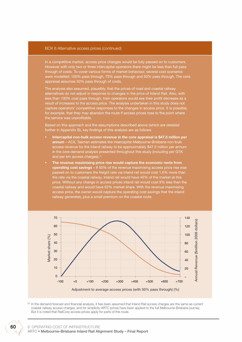
8. OPERATING COST OF INFRASTRuCTuREARTC Melbourne–Brisbane Inland Rail Alignment Study – Final Report
60
In a competitive market, access price changes would be fully passed on to customers. However with only two or three intercapital operators there might be less than full pass through of costs. To cover various forms of market behaviour, several cost scenarios were modelled: 100% pass through, 75% pass through and 50% pass through. The core appraisal assumes 50% pass through of costs.
The analysis also assumed, plausibly, that the prices of road and coastal railway alternatives do not adjust in response to changes in the price of Inland Rail. Also, with less than 100% cost pass through, train operators would see their profit decrease as a result of increases to the access price. The analysis undertaken in this study does not capture operators’ competitive responses to the changes in access price. It is possible, for example, that they may abandon the route if access prices rose to the point where the service was unprofitable.
Based on this approach and the assumptions described above (which are detailed further in Appendix B), key findings of this analysis are as follows:
Intercapital non-bulk access revenue in the core appraisal is $47.5 million per annum – ACIL Tasman estimates the intercapital Melbourne-Brisbane non-bulk access revenue for the inland railway to be approximately $47.5 million per annum in the core demand analysis presented throughout this study (including per GTK and per km access charges).28
The revenue maximising price rise would capture the economic rents from operating cost savings – If 50% of the revenue maximising access price rise was passed on to customers the freight rate via inland rail would cost 1.6% more than the rate via the coastal railway. Inland rail would have 45% of the market at this price. Without any change in access prices inland rail would cost 9% less than the coastal railway and would have 62% market share. With the revenue maximising access price, the owner would capture the operating cost savings that the inland railway generates, plus a small premium on the coastal route.
BOX 8 Alternative access prices (continued)
28 In the demand forecast and financial analysis, it has been assumed that Inland Rail access charges are the same as current coastal railway access charges, and for simplicity ARTC prices have been applied to the full Melbourne-Brisbane journey. But it is noted that RailCorp access prices apply for parts of this route.
-100 +0 +100 +200 +300 +400 +500 +600 +700–0
2010
4020
6030
8040
10050
120
140
60
70
Mar
ket
shar
e (%
)
Ann
ual R
even
ue ($
mill
ion
2008
do
llars
)
Adjustment to average access prices (with 50% pass through) (%)

8. OPERATING COST OF INFRASTRuCTuREARTC Melbourne–Brisbane Inland Rail Alignment Study – Final Report
61
Improved Inland Rail services and lower operating costs are expected to compensate for a higher access price – If there is some pass through of access cost increases from train operators to freight customers, then the premium over current coastal access charges which could be charged by the inland railway is shown below:
Annual non-bulk, intercapital revenue per annum at the revenue maximising access price is estimated as:
The revenue maximising access price is greatly impacted by elasticity assumptions – Undertaking this analysis using higher elasticities (as implied by ARTC demand modelling) results in higher access revenue available to the track operator because the service characteristics are valued much more highly (see Appendix B for further detail).
-100 0 100 200 300 400 500 600 700 800
–
20
40
60
80
100
120
140
Ann
ual R
even
ue ($
mill
ion
2008
do
llars
)
Percentage change to access price (%)
Revenue maximising price rise
100% passthrough = 126%75% passthrough = 177%50% passthrough = 278%
$– $3.09 $6.17 $9.26 $12.35 $15.43 $18.52 $21.60 $24.69
–
20
40
60
80
100
120
140
Ann
ual R
even
ue ($
mill
ion
2008
do
llars
)
Revenue maximising price per ‘000 gtk
100% passthrough = $6.9475% passthrough = $8.5250% passthrough = $11.67
$27.78
Price ($)

9. Above rail operational benefits
9. ABOVE RAIL OPERATIONAL BENEFITSARTC Melbourne–Brisbane Inland Rail Alignment Study – Final Report
62

9. ABOVE RAIL OPERATIONAL BENEFITSARTC Melbourne–Brisbane Inland Rail Alignment Study – Final Report
63
9. Above rail operational benefitsThis chapter presents the outcomes of train operation modelling which have been used to estimate train operating costs. It then compares estimates of train operating costs for Inland Rail with those for the coastal route.
Train operating costs on the inland railway are not included in the financial appraisal because it was undertaken on a below-rail basis and from the viewpoint of a track operator. However train operating costs are an important input in the analysis of the project’s economic benefits. As such the findings presented in this chapter are significant in the economic appraisal of Inland Rail. Further detail of the train operation modelling is presented in Appendix G.
9.1 Train operations
Assumptions have been made about the intermodal container trains that might operate on the inland railway. Drawing on the latest intermodal rail freight practices, an Inland Rail ‘reference train’ was developed and its specifications were used to inform both alignment design and the financial and economic modelling. The reference train is described as a ‘superfreighter’ to indicate that the type of train and market being served is similar to the premium services currently offered on the interstate network.
Achieving a journey time that provides opportunities for reduced costs in comparison to the existing coastal route is a key aspect of the study. Since neither the reference train nor the chosen corridor currently exist, a computer model of the train and the alignment was built using the RailSys train modelling tool to simulate journey time and the location of passing loops.
The data used to build the RailSys model of the final alignment came from a number of sources including ARTC data about the north-south corridor after upgrading has occurred; existing published data about the country and ARTC-leased network in NSW; data for new alignments generated in the course of the study; published wagon and train data; and knowledge of the latest type of alternating current (AC) traction diesel locomotives on intermodal trains in Australia.
Notional timetables were written to estimate the likely journey times once passing manoeuvres and operational procedures were added to transit times, and to test the methodology used to calculate the number of passing loops required to carry the estimated traffic.
To inform the economic and financial evaluation of the proposed route, estimates of a range of above rail (train operating) costs were made once the train, route and journey time characteristics were known.
9.1.1 Journey time results
Two possible timetables were written for the inland railway, representing different traffic volumes and routes according to the staged construction discussed in section 7.1:
Traffic volumes in 2020, with staged upgrades and deviations not completed
Traffic volumes in 2050, with proposed alignment construction completed, but with higher freight and train volumes using the railway.
The average journey times for the two timetables scenarios are shown below.
TABLE 22 Average Melbourne to Brisbane journey times
Average journey time (hours)
Initial route, 2020 traffic 20:21
Final route, 2050 traffic 20:26
Adding other traffic to the timetable would have minimal effect on superfreighter journey times because one of the major advantages of the inland railway is that superfreighter traffic can have priority over almost all other traffic on the route.
9.1.2 Passing loops
The timetabling exercise assumed that upgrades had taken place in accordance with strategies published by ARTC, including construction of continuous double track between Melbourne and Junee.
Loop spacing between Illabo and Oakey (west of Toowoomba) was determined using the characteristics of superfreighter trains. Between Oakey and Acacia Ridge coal traffic is expected to be significant, and here the different characteristics of coal trains were also taken into account.
The timetable was used to determine the number of loops required for the inland railway. In all, 32 new loops for superfreighters would be required from Parkes (Goobang Junction) to Brisbane (Acacia Ridge), and the double track section between Helidon and Laidley would be retained. This infrastructure would provide superfreighter journey times as estimated in the timetable exercise plus give flexibility for realistic service planning and recovery from delays.

9. ABOVE RAIL OPERATIONAL BENEFITSARTC Melbourne–Brisbane Inland Rail Alignment Study – Final Report
64
9.2 Inland Rail train operating costs
Train operating costs relate mainly to train crewing, rollingstock maintenance and fuel.
Crew costs and rollingstock maintenance costs were extrapolated from past trends and applied to likely Inland Rail operating scenarios. Fuel costs were estimated specifically for the chosen inland railway alignment because fuel consumption is highly dependent on the alignment traversed by the train.
Fuel consumption per train per trip was calculated for the reference train using RAMASES, a computer program designed for the task. Fuel consumption was estimated using base data gathered during Halcrow’s work to bring the first 3,220 kW AC drive locomotives into service in Australia. These locomotives are now being used on long distance intermodal freight services.
As with capital and track operating costs presented in previous chapters, the train operating costs presented in Chapter 9 are all inclusive of profit margins.
9.2.1 Crew costs
Crew costs were estimated using typical industry costs and assumed that each crew consisted of two people. It was assumed that they would be accommodated overnight before working a train back to their home depot the following day.
For a 20.5 hour journey, the cost is estimated to be $6,540 per trip (2010 dollars).
It was assumed that no new train crew depots are required for the inland railway.
9.2.2 Rollingstock maintenance costs
Locomotives can be assumed to run 250,000 km per year. The total cost of maintaining a mainline locomotive during its economic lifetime was estimated at $1.50 per km (2010 dollars).
Assuming a length of 1,731 km, the three locomotives on the reference train were allocated a total of $7,790 of the lifetime locomotive maintenance costs for a single Inland Rail trip.
Container carrying wagons were assumed to run 125,000 km per year. The total cost to maintain these wagons in mainline operational service during their economic lifetime was estimated at $0.05 per km (2010 dollars).
The 73 wagons on the reference train were allocated a total of $6,318 of the lifetime wagon maintenance costs for a single Inland Rail trip.
9.2.3 Fuel
The power and resistance characteristics of the reference train were estimated using industry data gathered from Australia and overseas. Alignment distances, speed limits, gradients, and the length and radius of curves were obtained from ARTC data and from the study alignment designs. The data was input to RAMASES which simulated the running of a train over an alignment.
From the power estimates produced by RAMASES, the amount of fuel required was estimated using fuel consumption figures derived from previous studies together with engine supplier data for locomotives operating at various speeds and hauling trains over various grades and curves. The fuel consumption figures are expressed in litres per trip and litres per Gross Tonne Kilometre x 1,000 (L/gtk).
Many factors cause the fuel consumption of a given train to vary significantly. Locomotive combination, load of the train, gradients, curves, driving style, wind resistance of the load and crosswinds are all significant as well as the number of times a freight train stops and accelerates back to line speed. Because these factors can vary consumption figures by up to 20%, no exact figure can be given train for a given route. A typical average was therefore estimated.
Fuel consumption for a typical northbound reference train (comprising 3 locomotives and 4,456 trailing tonnes) was estimated to be around 33,433 litres, which represents approximately 3.97 L/gtk. For an average north and southbound trip, this is estimated as 3.89 L/gtk reflecting that less tonnes are generally carried on a southbound train.
9.2.4 Train operating costs
The combined crew, rollingstock maintenance and fuel costs are shown in the table below per trip between Melbourne and Brisbane.

9. ABOVE RAIL OPERATIONAL BENEFITSARTC Melbourne–Brisbane Inland Rail Alignment Study – Final Report
65
TABLE 23 Inland Rail train operating cost per trip (2010 dollars)
Operating costs Estimated cost per trip
Crew cost $6,540
Rollingstock maintenance cost: locomotive container wagon
$7,790 $6,318
Fuel $27,750
Total $48,398
9.3 Comparison with coastal railway train operating costs (above rail benefits)
Table 24 on the next page provides a comparison of train operating costs on the inland and coastal railways. This is based on the analysis discussed above and information provided by ARTC on the coastal railway. It also describes the method used to estimate coastal railway costs relative to the inland railway estimates discussed above.
The table shows that train operating costs on the Inland Rail are estimated to be lower than on the coastal railway on per tonne and ntk basis. This suggests train operators would obtain above rail benefits by using Inland Rail rather than the coastal railway.

9. ABOVE RAIL OPERATIONAL BENEFITSARTC Melbourne–Brisbane Inland Rail Alignment Study – Final Report
66
TABLE 24 Inland versus coastal railway train operating costs (2010 dollars)
Cost item Inland railway Coastal railway Assumptions
Fuel consumption 3.89 litres per thousand gtk (average north and southbound)
(Per train: $14.05/km $0.0058/ntk)
4.45 litres per thousand gtk (average north and southbound)
(Per train: $11.82/km $0.0068/ntk)
Inland – for the 1,731km between Melbourne and Brisbane, each train estimated to use approximately 3.89 litres of fuel per gtk based on modelling of each track section. This is based on an average north and southbound train carrying 4,370 gt (train load including locomotives).
Coastal – the route via Sydney is approximately 1,904 km in length. Due to the additional grades and terrain traversed between Cootamundra, Sydney and Maitland, each north and southbound train is likely to average approximately 4.45 L/gtk. This is based on an average of 3,216 gt per train (including locomotives).
Assumes each train is fuelled mid way en route and subjected to the same amount of stops even though the route via Sydney is longer with the potential for more delays. Also assumes a resource price for diesel (excluding GST and excise) that was applied to convert to $/ntk.
Train crew costs* $5,945 per Melbourne– Brisbane trip
(Per train: $3.43/km $0.0014/ntk)
$8,121 per Melbourne–Brisbane trip
(Per train: $4.27/km $0.0024/ntk)
Inland – assumes two people per crew, and includes all crew-related costs.
Coastal – assumes two people per crew, with costs higher relative to inland railway based on transit time differential.
Rollingstock maintenance–locomotive costs
$1.36 per km per loco
(Per train: $4.50/km $0.0019/ntk)
$1.36 per km per loco
(Per train $4.50/km $0.0026/ntk)
Inland – based on the life of a 3,400 kW AC locomotive in service on Interstate Intermodal traffic, covering 250,000 km per year. There are three such locomotives on each reference train.
Coastal – assumes there are also three locomotives on each coastal train (assuming more than the current average of around 2.5 as Inland Rail is assumed to commence operations in 10–30 years time).
Rollingstock maintenance–container wagon costs
$0.05 per km per wagon
(Per train: $3.65/km $0.0015/ntk)
$0.05 per km per wagon
(Per train: $3.15/km $0.0018/ntk)
Inland – for the life of a typical container carrying bogie wagon in service on Interstate Intermodal traffic, covering 125,000 km per year. There are 73 such wagons on each reference train.
Coastal – based on information provided by ARTC. Assumes a coastal train comprises 18 generic ‘5-pack’ articulated wagons that carry 10 single-stack TEu. These wagons have 6 bogies whereas each Inland Rail wagon has 2 bogies. To apply the maintenance costs to a comparable wagon type, the number of coastal wagons was adjusted by a factor of (6/2) to reflect this (i.e. suggests 63 coastal wagons on a comparable basis with Inland Rail wagons).

9. ABOVE RAIL OPERATIONAL BENEFITSARTC Melbourne–Brisbane Inland Rail Alignment Study – Final Report
67
Cost item Inland railway Coastal railway Assumptions
Annual rollingstock depreciation and return on economic capital (economic cost of capital)
$18,191 per trip
(Per train: $10.51/km $0.0043/ntk)
$22,138per trip
(Per train: $11.63/km $0.0066/ntk)
Inland – based on indicative capital costs for a new locomotive of $5.5 million and a new wagon of $150,000, assuming there are 3 locomotives and 73 wagons per train. Also assumes rollingstock asset life of 20 years and interest rate of 7%. The number of trips travelled per annum was linked to transit time, and assumes faster turnaround time of locos than wagons.
Coastal – same cost, interest and depreciation rates, etc. applied, but assumes 3 locomotives and 63 wagons per trip (after adjusting wagon numbers for the number of bogies). The number of trips travelled per annum is lower relative to inland railway due to longer transit time.
Administration and management
Per train: $3.61/km $0.0015/ntk
Per train: $3.54/km $0.0020/ntk
Assumed to comprise 10% of total costs per ntk for both railways.
Total (exc. profit margin)
$40/km $0.0163/ntk $28/tonne
$39/km $0.0222/ntk $42/tonne
Per ntk cost is applied to ntk demand projections to estimate operating cost savings in the economic appraisal. Per tonne cost is also considered in the demand projections as part of freight costs.
* Some costs do not align with those in previous chapters as profit margin has been excluded for the economic appraisal.
Note: Average load (60% fronthaul and 40% backhaul) assumed in these costs is 2,432 nt/train (payload inc. container weight), 3,968 trailing tonnes/train (trailing tonnes inc. container and wagon but not loco weight) and 4,370 gt/train (train load inc. locos) for the inland railway. For the coastal route, a theoretical train was estimated by ARTC (after coastal route upgrades so with greater tonnage than the current actual average) that averages 1,749 nt, 2,820 trailing tonnes and 3,216 gt. The lower coastal railway load is linked to its single stacked rollingstock and shorter trains compared to double stacked, longer trains assumed on the inland railway.
TABLE 24 Inland versus coastal railway train operating costs (2010 dollars) cont...

C. Financial and economic appraisal 10. Financial analysis
10. FINANCIAL ANALYSISARTC Melbourne–Brisbane Inland Rail Alignment Study – Final Report
68

10. FINANCIAL ANALYSISARTC Melbourne–Brisbane Inland Rail Alignment Study – Final Report
69
10. Financial analysisThe financial analysis presented in this chapter examines the Inland Rail project to determine whether it is expected to be financially viable on a commercial basis, from the perspective of a track operator that is a standalone commercial entity. without any government or other external financial support. It also presents a basis for evaluating private sector involvement in the project, considering four financing scenarios.
10.1 Financial feasibility
This chapter assesses the financial feasibility of the Inland Rail project before financing (i.e. it excludes financing cash flows as they are more relevant for analysis of specific financing structures). The purpose of this analysis is to determine whether the revenues are sufficient to cover the capital and ongoing costs for the project, with the analysis period being from 2020, 2030 or 2040, operating until 2070. The analysis is based on nominal cash flows discounted using a pre-tax, project weighted average cost of capital (WACC) of 16.6% to a base date of 1 January 2010.
The following has been assumed in relation to private ownership and delivery of Inland Rail:
South of the NSW/Queensland border, the inland railway traverses track that is mostly leased long-term by ARTC. North of the border, part of the railway would traverse track, or a rail corridor, owned by QR (Rosewood–Kagaru) and leased long-term by ARTC (Kagaru–Acacia Ridge).30 As a result a spectrum of ownership possibilities, funding and operational control roles for the inland railway, and different delivery options could be adopted for different sections of the track. However it has been assumed that one delivery option would be adopted for the full length of the inland railway from Illabo to Kagaru
Access revenue and infrastructure maintenance costs for track from Melbourne to Illabo, and Kagaru to Acacia Ridge, accrue to ARTC only as part of the coastal railway and have therefore not been allocated to Inland Rail. The impact of this is that while the inland railway is 1,731 km between South Dynon and Acacia Ridge, the Inland Rail business is assumed to comprise the 1,220 km between Illabo and Kagaru
Access revenue and below rail maintenance costs for that part of the route that uses corridor owned by QR between the NSW/Queensland border and Kagaru has been assumed to accrue to Inland Rail. It has been assumed that this corridor would be leased from QR based on an annual peppercorn rent as the Inland Rail project would upgrade and convert significant sections of the corridor to dual gauge, with a 4,530 m long tunnel beneath Toowoomba
In line with the terms of reference in Box 2, the study focuses on a project-specific analysis of Inland Rail. While it is acknowledged there are relationships between the coastal and inland railways (as has been captured in the demand analysis and economic appraisal), a detailed financial appraisal of both lines concurrently as options for freight capacity is beyond the scope of this study. As a result, the financial appraisal has assessed the feasibility of Inland Rail as a standalone project, assuming it is a separate entity and does not receive any external financial support. Further, it does not consider losses to ARTC resulting from a reduction of coastal railway freight (which is considered in section 12.2.1).
The analysis suggests that Inland Rail will not generate sufficient access revenue relative to costs to make it financially viable on a commercial basis. Indeed, the total nominal capital and operating costs exceeded the total nominal track access revenues, regardless of the assumed operational start date of 2020, 2030 or 2040. As shown in Table 25, the net present values (NPV) for Inland Rail cash flows (before financing) are negative for each operational start date.
Table 25 indicates that below rail revenue is not sufficient to recover the significant capital outlay required for construction of the inland railway. It shows that Inland Rail has better financial performance by delaying its operation for 10 or 20 years as demand for the railway increases over time. However, improved results for delayed commencement of operations are also affected by costs and revenue being discounted over a longer period. The table also indicates that Inland Rail has positive operational cash flows, i.e. if capital costs are excluded.
The negative project net present values in the table above are lower than possible subsidy requirements for the railway as the financial cashflows exclude interest, return on equity and other financing costs required to fund the capital and operating expenditure.
30 ARTC 2010, Queensland standard gauge rail line – leased to ARTC, available at: http://www.artc.com.au/Article/Detail.aspx?p=6&np=4&id=260

10. FINANCIAL ANALYSISARTC Melbourne–Brisbane Inland Rail Alignment Study – Final Report
70
TABLE 25 Financial – project NPV (pre tax) nominal cash flows ($ million, 2010 dollars, discounted, excluding financing costs)
Financial results Operations commence:
2020 2030 2040
Capital cost -2,112 -705 -235
Infrastructure operating revenue 260 96 34
Infrastructure operating cost -75 -26 -8
Project NPV – operating cash flows only (excluding capital costs) 185 71 26
Project NPV – total project cash flows -1,927 -634 -209
Note: Excludes financing cost (debt and equity). Figures in this table may not total due to rounding.
General financial appraisal assumptions
The general assumptions used in the project NPV appraisal are presented in Table 26.
TABLE 26 General financial appraisal assumptions

10. FINANCIAL ANALYSISARTC Melbourne–Brisbane Inland Rail Alignment Study – Final Report
71
Assumption Details Notes
Analysis period Through to 2070 Thirty years after the last scenario begins full operations, with base year in 2010
Concession period 2020: 50 years 2030: 40 years 2040: 30 years
Length of the concession is relatively long to maximise time to earn a return
Construction period 5 years Period assumed for the construction of the inland railway track assets, with capital costs allocated on an S-curve basis
Cost and revenue base date
2010 Has the same basis as the economic analysis and uses assumptions provided by technical consultants
Net present value (NPV) date
January 2010 Base date for the calculation of the NPV of cash flows of the project, discounted at the beginning of the period
Capital cost 2010 dollars escalated by Producer Price Index
Capital cost assumptions were estimated in 2010 dollars. For the purpose of the financial appraisal, these assumptions were escalated in the financial model by the average historical producer price index (for road and bridge construction) of 4.23% pa31
Operating cost and revenue estimates
2010 dollars escalated by CPI
Key revenue and cost assumptions were estimated in 2010 dollars. For the purpose of the financial appraisal, these assumptions were escalated in the financial model using CPI where applicable
Consumer Price Index (CPI)
3.0% upper end of Reserve Bank of Australia (RBA) target range
Basis of cash flows for financial analysis
Nominal For the purposes of the financial appraisal, the cash flows in the financial model are in nominal terms
Project discount rate (Nominal, Pre tax)
16.59% The recent Weighted Average Cost of Capital (WACC) regulatory determination of the Australian Competition and Consumer Commission (ACCC) determination for the ARTC’s interstate network was 11.61% post tax, nominal32
For the purpose of the project NPV analysis, our approach was to convert this to a pre tax discount rate applying an average tax rate of 30%. This results in a nominal, pre tax discount rate of 16.6%
Capital Costs ($ million, undiscounted, unescalated)
$4,701.3 (P90) Capital costs expressed in 2010 dollars (unescalated for real and nominal increases, and undiscounted) including a 18% contingency
PV Capital Costs ($ million, discounted, escalated)
2020: $2,113 2030: $705 2040: $235
The PV of capital costs calculated using a discount rate of 16.6%, and a base date of 1 January 2010
Demand inputs Refer Chapter 3 & Appendix B
Demand projections for the inland railway prepared by ACIL Tasman for use in the financial appraisal
Track access pricing Refer Chapter 8 Access charges were assumed to be in line with current coastal rail prices
Construction and operating costs
Refer Chapters 7, 8 and 9
Costs were estimated for the inland route by the LTC
Depreciation rates – track components
3.33% Assumed average useful life of track components 30 years33
Sensitivity analysis
31 Australian Bureau of Statistics (ABS) 2009, Cat. No. 6427.0: Producer Price Indexes, Australia: Table 15. Selected output of division E construction, group and class index numbers, ‘Road and bridge construction Australia’ (Sept 1999-Sept 2009) ACCC
32 ACCC 2008, Final Decision: Australian Rail Track Corporation Access Undertaking – Interstate Rail Network, July 2008, p 164
33 ACCC 2008, Final Decision: Australian Rail Track Corporation Access Undertaking – Interstate Rail Network, July 2008

10. FINANCIAL ANALYSISARTC Melbourne–Brisbane Inland Rail Alignment Study – Final Report
72
The table below presents a range of sensitivity tests performed to understand the impact of changes in key variables on financial outcomes.
TABLE 27 Financial sensitivity analysis ($ million, discounted, 2010 dollars)
Inland Rail Financial NPV Operations commence:
2020 2030 2040
1. Core appraisal (16.6% discount rate) -1,927 -634 -209
2. Discount rate reduced to 14.6% Pre tax, Nominal -2,128 -830 -325
3. Discount rate increased to 18.6% Pre tax, Nominal34 -1,736 -483 -134
4. Demand reduced by 30% -2,001 -659 -219
5. Demand increased by 30% -1,859 -607 -199
6. Capital costs decreased by 30% -1,294 -423 -138
7. Capital costs increased by 30% -2,561 -846 -280
8. Demand with more sensitive elasticity assumptions – ARTC elasticity assumptions were applied as they were more sensitive than those obtained from ACIL Tasman freight customer surveys (see Box 5)
-1,883 -613 -201
9. Alternative rail access price based on road/rail access price analysis – analysis was undertaken concurrently with this study to understand the impact on road and rail competitiveness from changes in government pricing policy. The impact on Inland Rail from alternative pricing policies are assessed:
9a. Road pricing based on depreciated optimised replacement cost (DORC) values / Rail pricing as status quo – heavy vehicle road pricing is currently based on a pay-as-you-go (PAYGO) approach. A shortcoming of this approach is that the cost base may be understated. This could be addressed if road pricing was based on DORC values for road assets. This scenario tested the impact on Inland Rail if road applied a DORC pricing approach, assuming the current allocation of costs to heavy vehicles and rail priced as per the current rail regime
-1,910 -627 -206
9b. Road pricing based on PAYGO with higher heavy vehicle cost allocation / Rail pricing based on current ARTC access charges – a further shortfall of the current road approach is that the proportion of the road cost base allocated to heavy vehicles may be understated. To test this, adaptations to current road PAYGO were assumed by increasing the heavy vehicle allocation of total road costs (34.5% compared to current 23.3% for the Melbourne–Brisbane road network)
-1,919 -632 -207
9c. Road pricing based on DORC / Rail pricing on DORC including a return on contributed assets – this scenario tested a more equal pricing regime. It assumed road user charges based on DORC and current National Transport Council (NTC) allocation of costs to heavy vehicles, and rail access charges based on DORC including a return on contributed assets (i.e. included rail assets funded from government contributions, that would not be included in the current rail pricing regime)
-1,497 -447 -138
10. High oil price – an oil price of uS$200/barrel was assumed in comparison to uS$120 in the core appraisal. An increase in fuel prices affects road freight more than rail freight, and was assumed to pass through to freight rates
-1,921 -633 -208
11. Change in GDP growth
11a. High GDP – core appraisal assumed low GDP growth in 2010 and 2011, moving up to 3.1% pa from 2013. This scenario tested GDP growth of 3.6% pa from 2013
-1,916 -627 -204
11b. Low GDP – this scenario tests lower GDP growth forecasts of 2.6% pa from 2013
-1,927 -634 -209
The figure below presents the sensitivity results graphically.34 In the discount rate sensitivity tests, a higher discount rate results in lower financial viability and a lower discount rate results in higher financial viability. This is due to the sheer scale of the capital costs relative to revenues. For example, at a discount rate of 14.6% relative to the 16.6% core rate, the PV of revenues becomes more positive and the PV of capital costs becomes more negative, with the scale of the increased capital costs dominating the final NPV.

10. FINANCIAL ANALYSISARTC Melbourne–Brisbane Inland Rail Alignment Study – Final Report
73
FIGuRE 21 Chart comparing financial sensitivity results for Inland Rail assuming operations commence in 2030 ($ million, discounted, 2010 dollars)
Key findings of this sensitivity analysis are that Inland Rail does not achieve financial viability under any scenario:
Financial NPV remains negative even when tests are performed such as reducing capital costs by 30%, increasing demand by 30%, and adjusting road pricing so that a greater portion of costs are allocated to heavy vehicles
The test with the most negative effect on the financial results was an increase in capital costs of 30%
The test that had the most positive effect on financial results was to reduce capital costs by 30%
Following this, the test with the second most positive impact on results was a change the basis of road and rail pricing so that both road and rail pay prices based on depreciated optimised replacement cost. This change in the pricing regime resulted in an increase in the access price for Inland Rail and a more even spread of demand between road and rail.
Sen
sitiv
ity t
est
Project NPV ($ millions)
-900 -800 -700 -600 -500 -400 -300 -200 -100 0
1
2
3
4
5
6
8
9a
9b
9c
10
11a
11b

10. FINANCIAL ANALYSISARTC Melbourne–Brisbane Inland Rail Alignment Study – Final Report
74
10.2 Private and public sector delivery options
One of the objectives of the study is to determine a basis for evaluating the level of private sector support for the project (see Box 2).
There is a spectrum of delivery options with differing levels of possible private sector involvement. Private sector involvement in the inland railway project could include:
Construction
Design
Maintenance
Financing
Operation
Train operation/maintenance.
Table 28 presents a range of options along the spectrum.
In addition to the phases of infrastructure delivery shown below, train operations could be provided by either the private or public sectors. For the purpose of this study, it is assumed that the private sector would operate the trains and that these would use Inland Rail.
Financing options
For each of the delivery options, there is a range of possible funding options. Funding options for the public and private sectors are discussed in Table 29.
TABLE 28 Delivery options
Delivery option Construct Design Maintain Finance Operate (track only)
Construction contract Private Government Government Government Government
Design and Construct Private Private Government Government Government
Design, Build, Maintain, Transfer Private Private Private Government Government
Privately financed project (PFP) Private Private Private Private Private
TABLE 29 Public/private sector funding options
Public sector Private sector
Public sector funding for Inland Rail may come from a number of options:
Government contributions: government funding may be acquired through federal and/or state budget allocations where the government contributes to the cost of the project, and where contributions are not repaid
Government equity contributions: government may provide assistance to the project through provision of equity. In some instances this can improve the financial viability of a project if government has a lower equity return target than the private sector
Government-sourced debt: government may provide assistance to the project by raising debt sourced at government rates. This may include a guarantee to debt providers to reduce risk.
Where the project is delivered partially or in whole by the private sector, possible sources of funding may include:
Debt sources: bank debt, mezzanine debt and bonds
Equity sources: project sponsors, superannuation funds, sovereign funds, private equity and initial public offering (IPO)
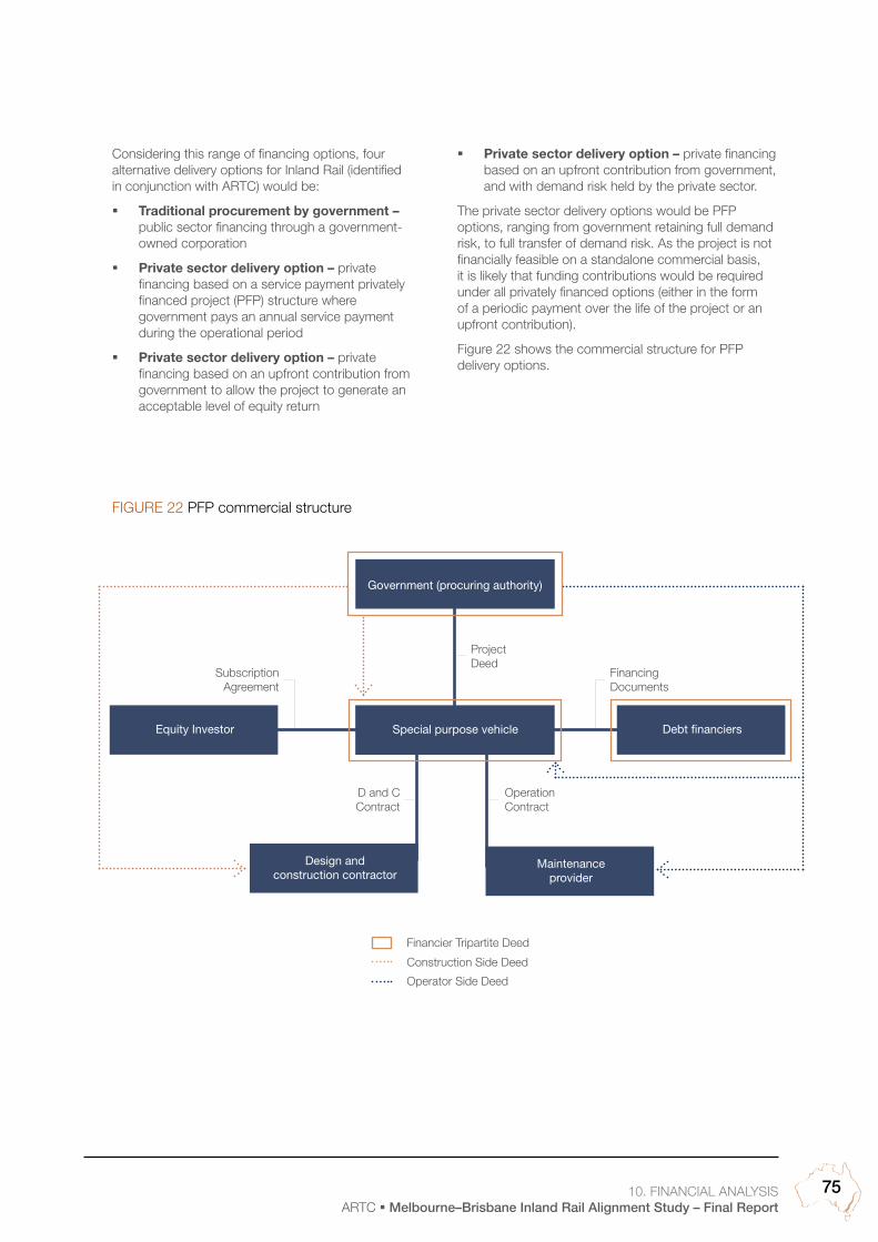
10. FINANCIAL ANALYSISARTC Melbourne–Brisbane Inland Rail Alignment Study – Final Report
75
Considering this range of financing options, four alternative delivery options for Inland Rail (identified in conjunction with ARTC) would be:
Traditional procurement by government – public sector financing through a government-owned corporation
Private sector delivery option – private financing based on a service payment privately financed project (PFP) structure where government pays an annual service payment during the operational period
Private sector delivery option – private financing based on an upfront contribution from government to allow the project to generate an acceptable level of equity return
Private sector delivery option – private financing based on an upfront contribution from government, and with demand risk held by the private sector.
The private sector delivery options would be PFP options, ranging from government retaining full demand risk, to full transfer of demand risk. As the project is not financially feasible on a standalone commercial basis, it is likely that funding contributions would be required under all privately financed options (either in the form of a periodic payment over the life of the project or an upfront contribution).
Figure 22 shows the commercial structure for PFP delivery options.
FIGuRE 22 PFP commercial structure
Design and construction contractor
Maintenance provider
Government (procuring authority)
Equity Investor Special purpose vehicle Debt financiers
Project Deed
Operation Contract
Financing Documents
D and C Contract
Subscription Agreement
Financier Tripartite Deed
Construction Side Deed
Operator Side Deed

10. FINANCIAL ANALYSISARTC Melbourne–Brisbane Inland Rail Alignment Study – Final Report
76
Optimal approach
Because the project will not economically or financially viable for some time, it would not be appropriate at this stage to choose an optimal approach for delivery and operation of the railway. Approaches for private and public sector partnership change over time, and are likely to be different in 2020 or 2030 compared with today. While there is likely to be private sector interest in a design and construct (D&C) arrangement, the market appetite for PFP options involving private sector demand risk in 10-30 years would be more readily understood through market testing closer to that time. As such, the financial appraisal is not specific to either private or public sector delivery/financing/operation. In particular, financing costs have been excluded as these are most impacted by the level of private sector involvement.
10.3 Key issues affecting delivery options
10.3.1 Market appetite for demand based projects
Market appetite for projects where the private sector takes on demand risk, compared to projects based on service payments whereby government essentially holds this risk, depends on the level and nature of risks that the market is willing to accept. It appears that a shift in market preference away from demand-based projects to service payment projects has occurred in Australia in recent times, in particular in the toll road sector. There is a strong history of toll roads being delivered under a Build, Own, Operate Transfer (BOOT) model, with full transfer of demand risk to the private sector. The performance of rail lines such as Alice Springs-Darwin and toll roads such as Sydney’s Cross City Tunnel and Lane Cove Tunnel appears to have caused the private sector to reconsider its willingness to accept demand risk. The Peninsula Link project currently in procurement in Victoria has been structured as an availability payment based project.
10.3.2 Financial markets
The Global Financial Crisis (GFC) caused a global liquidity crisis which resulted in reduced appetite to fund infrastructure, reduced lending maturities, conservative refinancing assumptions and an increase in margins.
However, market activity indicates that the severity of the GFC peaked in February/March 2009 and that conditions in financial markets have since improved. Recent indications are that a greater level of confidence of lenders has emerged.
The movement in financial markets over the past 12 months demonstrates the volatility of international and domestic markets. Activity in financial markets is cyclical and it is very difficult to forecast movements in the medium to long term. Given the timeframe for this project (commencing operations in 2020, 2030 or 2040), it is not
possible to predict where financial markets will be in the cycle when the project requires financing in 10–30 years.
10.4 Approach to evaluating delivery options
A set of evaluation criteria has been developed along with assigned weightings that could be used to assess delivery options. Applying this approach, the delivery options would be scored against each evaluation criterion and ranked according to the resultant total weighted scores. The evaluation criteria have been developed based on the government objectives and the attributes of projects suitable for private financing (refer National Public Private Partnership Guidelines: Volume 1–Procurement options analysis, December 2008). The criteria are indicative only, and would be considered in more detail closer to the time of financing construction of the inland railway. The evaluation criteria are:
1. Risk management – the extent to which each delivery option provides incentives to manage and reduce risks and transfers risk from the government to the private sector
2. Market interest – the extent to which each delivery option assists in maximising market interest (and therefore competition) amongst the private sector parties (construction companies, financiers, operators) with the skills, expertise and capacity required to deliver the project
3. Innovation and efficiency – the extent to which the delivery option is likely to foster innovation in construction and operations, delivering time and cost efficiencies with relation to the development and operations of the inland railway and adopting a whole of life costing approach
4. Financial feasibility – the cost to government
5. Budget certainty – the extent to which each delivery option assists the government in accurately forecasting its revenue and expenditure streams
6. Stakeholder management – the extent to which each delivery option is likely to be preferred by stakeholders and therefore minimise the required level of stakeholder management undertaken by government.
The evaluation criteria set out above have been allocated an indicative weighting by the study team in consideration of their potential significance from government’s perspective. However, government objectives and the weightings applied to each may be different at the time a decision is to be made on the project. The financial feasibility criterion has not been allocated a weighting as the ranking for this item would be determined directly from financial appraisal results for different options. Table 30 sets out a scoring scale that could be used to assess the delivery options against the evaluation criteria.

10. FINANCIAL ANALYSISARTC Melbourne–Brisbane Inland Rail Alignment Study – Final Report
77
TABLE 30 Indicative assignment of weightings to criteria
Criteria Weighting (%)
Qualitative criteria
Risk management 30
Market interest 30
Innovation and efficiency 15
Budget certainty 15
Stakeholder management 10
Financial criteria
Net cost to government (NPV) Not applicable
Table 31 sets out a scoring scale to assess the delivery options against the evaluation criteria.
TABLE 31 Indicative scoring scale
Level of satisfaction of the evaluation criteria by the option Score
High 5
Moderate to High 4
Moderate 3
Low to Moderate 2
Low 1

11. Economic analysis
11. ECONOMIC ANALYSISARTC Melbourne–Brisbane Inland Rail Alignment Study – Final Report
78

11. ECONOMIC ANALYSISARTC Melbourne–Brisbane Inland Rail Alignment Study – Final Report
79
11. Economic analysisAn economic appraisal of Inland Rail was undertaken to assess whether it is economically viable in contrast to the situation without an inland railway. This would aid future government and private sector evaluations and help guide efficient resource allocation.
The box below explains the difference between a financial appraisal (presented in Chapter 10) and an economic appraisal as presented in this chapter.
BOX 9 Financial versus economic evaluation
Investment evaluations conducted from the wider economy or community’s perspective are termed economic evaluations whereas those evaluations conducted from the producer’s perspective only (e.g. the track operator) are known as financial evaluations. This is an important distinction as the outputs have varying purposes:
Financial appraisal – Financial appraisals assess the financial viability of a project from the perspective of owners/operators (e.g. in this case, the potential track owner and operator of the inland railway). Financial appraisals are concerned only with the financial returns delivered to operator stakeholders and do not take into account the costs or benefits derived by other parties and the wider community. Financial costs and revenues include capital, operating and maintenance costs; and operation. In the case of Inland Rail, these are expected to include track access charges for the track operator (assuming separate track and train operations).
The aim of the financial appraisal in this study is to enable assessment of whether Inland Rail is viable from the perspective of a single commercial entity, based on financial revenues and costs.
Economic appraisal – Economic (cost benefit analysis) appraisals assess the total costs and benefits of a project to the community. As such, economic appraisals encompass the costs and benefits accrued and incurred by many different stakeholders, including the project proponents, users, government and the community in general. An economic appraisal takes into account costs and benefits that are not necessarily derived directly from market based transactions including, in this study of Inland Rail: value of freight travel time, reliability, accidents, and externalities and congestion. Economic evaluations also take into account the opportunity costs of resources used in the project. Consequently, taxes and subsidy payments are deducted as they simply represent transfer payments by government and do not represent the resource cost of producing a good or service.
The aim of the inland railway economic appraisal is to assess the project’s merits in terms of the economic efficiency of resource allocation and the quantification of total costs and benefits to the community.

11. ECONOMIC ANALYSISARTC Melbourne–Brisbane Inland Rail Alignment Study – Final Report
80
11.1 Cost benefit analysis methodology
11.1.1 CBA approach
This appraisal uses a rail freight cost benefit analysis (CBA) framework to assess the potential change in economic welfare with the inland railway.
The appraisal is broadly consistent with guidelines for CBA that are provided by the Australian Transport Council (ATC) in its 2006 National Guidelines for Transport System Management in Australia as well as those issued by Infrastructure Australia, various Australian jurisdictions,36 and other mode-specific guidelines prepared by organisations such as Austroads.
Key inputs to the economic appraisal
The CBA draws upon the following inputs:
Base Case and Inland Rail scenario definitions presented later in this chapter
Capital and operating cost assumptions as well as railway and train performance specifications based on LTC estimates as described in Chapters 4, 5, 7, 8 and 9 and Appendices C, G, J and K
ACIL Tasman freight forecasts as discussed in Chapter 3 and Appendix B.
Measures of economic performance
This CBA reports on the following measures of economic performance:
Net Present Value (NPV) – the difference between the present value (PV) of total incremental benefits and the present value of the total incremental costs. Scenarios that yield a positive NPV indicate that the incremental benefits of the project exceed the incremental costs over the evaluation period
Benefit Cost Ratio (BCR) – ratio of the PV of total incremental benefits over the PV of total incremental costs. A BCR greater than 1.0 indicates whether a project is also economically viable, as it presents a ratio of benefits relative to costs in present value (PV) terms. A BCR greater than 1.0 indicates PV benefits outweigh PV costs
Net Present Value: Investment Ratio (NPVI) – the NPV is divided by the PV of the investment costs (PVI). The NPVI measures the overall economic return in relation to the required capital expenditure
Economic Internal Rate of Return (EIRR) – the discount rate at which the PV of benefits equals the PV of costs. An IRR greater than the specified discount rate (default 7%) also indicates a project is economically worthwhile. However the IRR can yield ambiguous results if the streams of costs and benefits are not continuous over time. It is therefore commonly recommended that the IRR be used along with other measures.
11.1.2 Options considered
The demand projections, and both the economic and financial appraisals conducted for this project, address the following scenarios:
Base Case scenario – assumes there is no Inland Rail and freight travels by road or existing rail lines. It also assumes currently planned upgrades to the existing coastal railway proceed and that the Newell Highway will be upgraded to maintain capacity and performance levels
Inland Rail project scenario – this scenario assumes development of Inland Rail with a route length of 1,731 km and a terminal-to-terminal transit time of 20.5 hours. The scenario also assumes that upgrades to the coastal railway and Newell Highway will take place in line with the Base Case.
Table 32 summarises the route distances, capital costs and other assumptions of the Inland Rail scenario compared with the Base Case.
36 Jurisdiction-based guidelines include the Queensland Treasury 2006 Cost-Benefit Analysis Guidelines, Victorian Department of Transport (DoT) 2007, Guidelines for Cost-Benefit Analysis, the NSW Treasury 2007, NSW Government Guidelines for Economic Appraisal

11. ECONOMIC ANALYSISARTC Melbourne–Brisbane Inland Rail Alignment Study – Final Report
81
TABLE 32 Summary of assumptions for specific scenarios
Assumption Mode/route Base case (no Inland Rail)
Inland Rail
Capital costs (2010 dollars, $ million, undiscounted) (1)
Inland railway n/a $ 4,701.3 (P90, exc. profit margin, inc. contingency)
Coastal railway $3,011.0 $3,011.0
Road in corridor Assumed as equal under the two scenarios
Distance(M–B terminal-terminal), km
Inland railway n/a 1,731
Coastal railway 1,904 1,904
Road 1,650 (door-to-door) 1,650 (door-to-door)
Transit time(M–B terminal-terminal), hours
Inland railway n/a 20.5 hrs
Coastal railway 27.5 hrs37 27.5 hrs
Road n/a n/a
Transit time(M–B door-door), hours (2)
Inland railway n/a 25.5 hrs
Coastal railway 32.5 hrs 32.5 hrs
Road 23.5 hrs (3) 23.5 hrs
Reliability (M–B) Inland railway n/a 87.5%
Coastal railway 77% in 2015 77% in 2015
Road 98% 98%
Availability (M–B) Inland railway n/a 95%
Coastal railway 93% 93%
Road 98% (declining to 95%) 98% (declining to 95%)
Door to door price(M–B, relative to road)
Inland railway n/a 52.2% (declining to 48.8%)
Coastal railway 57.6% (declining to 53.6%)
57.6% (declining to 53.6%)
Road 100% 100%
Source: LTC cost and time estimates, and ARTC estimates for other rail capital costs.
Note: (1) capital costs include profit margin, which is excluded from costs in the economic appraisal; (2) the economic appraisal is undertaken on a ‘door-to-door’ basis; (3) 23.5 hours door-to-door transit time for road is based on assumption that 70% of trips have a transit time of 22 hours, and 30% will consolidate freight via an intermodal terminal (i.e. 22 hours plus 5 hour consolidation time). This results in a weighted average road transit time of 23.5 hours door-to-door. This was confirmed by industry estimates provided to ACIL Tasman. Slower road services might attract a price discount, which are not incorporated in the demand model.
37 ACIL suggests that the 27.5 hour transit time may be difficult to achieve as this would require three locomotives, which operators may not otherwise choose for haulage of a 1500m train. As such, this may be a conservative estimate for Inland Rail viability.

11. ECONOMIC ANALYSISARTC Melbourne–Brisbane Inland Rail Alignment Study – Final Report
82
The key characteristics distinguishing road and rail in the Melbourne–Brisbane corridor are presented graphically below in Figure 23.
The alternative road and rail options available to freight travelling along the Melbourne–Brisbane corridor are presented in Figure 24. These form the basis of the Base Case and Inland Rail scenario.
11.1.3 Base Case
In the Base Case, it is assumed that there is no inland railway and Melbourne–Brisbane freight continues to use existing road and coastal railway infrastructure. It assumes business as usual upgrading of the coastal route, the Newell Highway, port and intermodal terminal infrastructure, as described below:
Coastal railway upgrades
under the Base Case, it is assumed that ARTC’s planned upgrades on the coastal railway will take place, including the committed Stage 1 of the proposed Northern Sydney Freight Corridor Program ($840 million). This is presented in Table 33 on page 84 alongside the costs estimated to be delayed as a result of some traffic being diverted from the coastal route to the inland route (assuming Inland Rail commences operating in 2020).
ARTC planned upgrades on the coastal railway (excluding the Northern Sydney Freight Corridor Program) – ARTC has planned a range of expenditure on the coastal railway between 2010 and 2070, including:
à Loop extensions and new loops between Brisbane and Sydney
à Passing lanes between Brisbane and Sydney
à Southern Sydney Freight Line enhancement
à Duplication of Albury to Junee (see Table 33 for greater detail).
ARTC considers it may be possible to delay some coastal railway expenditure if there is an inland railway, as some passing lanes north of Maitland can be deferred if freight travelling between Melbourne and Brisbane is diverted to Inland Rail. The extent of delayed expenditure on the coastal railway is restricted as Melbourne/Adelaide/Perth–Brisbane freight is estimated to comprise around 28% of current train movements.38
North-south corridor projects announced for Federal Government investment in the 2010 Budget – in the Federal Government budget announced in May 2010, $1 billion of investment into ARTC was announced to build on existing investment strategies and deliver productivity benefits to the overall economy through investment in transport infrastructure. Of this total investment, approximately $300 million is relevant for the coastal railway so has been incorporated in both the Base Case and Inland Rail economic scenarios:
à North Coast Curve Easing: program to ease tight curves at 58 discrete sites on the North Coast. It aims to improve transit time through minor adjustments to the track, largely within the existing land corridor
à Goulburn, Moss Vale and Glenlee Double Track Passing Loops: provides passing loops on the double-track between Yass and Southern Sydney to facilitate overtaking moves
38 Provided by the Northern Sydney Freight Corridor project team.
FIGuRE 23 Characteristics of the Melbourne-Brisbane road and rail freight market
Note: This chart is illustrative only and is not to scale
Route length1,650km
95%
98%
23.5 hrs door-to-door
100% door-to-door
32.5 hrs door-to-door
53.6% door-to-door
25.5 hrs door-to-door
48.8% door-to-door
1,904km
93%
77%
1,731km
95%
87%
Availability
Reliability
Transit time
Freight price
Road
Coastal railway
Inland railway

11. ECONOMIC ANALYSISARTC Melbourne–Brisbane Inland Rail Alignment Study – Final Report
83
FIGuRE 24 Alternative road and rail routes between Melbourne and Brisbane
Note: The figure above presents the National Highway from Melbourne to Brisbane via Toowoomba, using the Gore Highway to Toowoomba then the Warrego Highway to Brisbane. It is noted that freight may travel on other routes in the area, for example via Warwick using the Cunningham Highway to Warwick and on to Brisbane.

11. ECONOMIC ANALYSISARTC Melbourne–Brisbane Inland Rail Alignment Study – Final Report
84
TABLE 33 ARTC proposed capital spend on the north-south corridor assumed in demand and appraisals ($ millions, undiscounted, 2010 dollars)
Coastal capital expenditure item
Potential year of capital spend
Base case (ARTC
demand)
Base case (ACIL
demand)
Inland Rail commencement date:
2020 2030 2040
Brisbane–Sydney, Northern Sydney Freight Corridor Program (Stage 1)
2010-2015 840.0 840.0 840.0 840.0 840.0
North south corridor Federal Government investment (2010 Budget)
2010-2013 300.0 300.0 300.0 300.0 300.0
Brisbane–Sydney 22 loop extensions & 4 new loops
2011 260.0 - - - -
2030 - 130.0 - - 130.0
2040 - 130.0 - - -
Beyond 2070 - - 260.0 260.0 130.0
Junee–Melbourne duplication, section Seymour–Tottenham
2013 300.0 - - - -
2030 - 300.0 300.0 300.0 300.0
Junee–Melbourne duplication, section Albury to Junee
2015 300.0 - - - -
2040 - 300.0 300.0 300.0 300.0
Brisbane–Sydney 17 passing lanes of 14 km each
2025 481.0 - - - -
2060 - 481.0 - - -
Beyond 2070 - - 481.0 481.0 481.0
Brisbane–Sydney 16 passing lanes of 14 km each
2028 480.0 - - - -
2070 - 480.0 - - -
Beyond 2070 - - 480.0 480.0 480.0
SSFL enhancement 2029 50.0 50.0 - 50.0 50.0
2039 - - 50.0 - -
Total (undiscounted) 3,011.0 3,011.0 3,011.0 3,011.0 3,011.0
Total (PV, discounted) 1,746.0 1,200.4 1,139.4 1,146.2 1,177.6
Saving relative to the ACIL Base Case
(PV, discounted) - - 61.0 54.2 22.9
Source: ARTC 2009 advice to PwC; Study team consultation with the Northern Sydney Freight Corridor Program team ; ARTC 2008, 2008–2024 Interstate and Hunter Valley Rail Infrastructure Strategy; NSW Government 2009, Budget 2009/10–Transport, 16 June 2009; and ARTC 2010, communications with PwC relating to the Federal Budget north south corridor investments, May 2010
Note: The ARTC base case is presented for comparative purposes only and is indicative of the difference between demand projections (see Box 10). This indicates that savings in coastal rail capital costs due to Inland Rail will be higher if there is a growth in traffic.

11. ECONOMIC ANALYSISARTC Melbourne–Brisbane Inland Rail Alignment Study – Final Report
85
à Rerailing Albury–Melbourne (as well as Melbourne–Geelong): involves rerailing 239 track km of rail and upgrading deficient bridges and turnouts.
These north-south corridor projects are expected by ARTC to result in a 44 minute transit time reduction northbound and 35 minute reduction southbound on the coastal railway between Melbourne and Brisbane, primarily linked to easing of curves on the north coast. As this investment was announced during the course of Stage 3 of the study it was incorporated into the final results in this report by assuming an average transit time saving of 30 minutes on the coastal railway. This was because the economic modelling does not distinguish between north and southbound, and also does not assess transit time below half an hour increments.39
Stage 1 of the Northern Sydney Freight Corridor Program – the Northern Sydney Freight Corridor Program is an initiative of the Australian Government to remove operational impediments to rail freight traffic between North Strathfield and Broadmeadow near Newcastle.40 There is a committed funding agreement in place between the Australian and NSW governments for Stage 1 of the Program ($840 million).
A further Stage 2 option is being considered by the Australian Government. However as these works have not been committed, they are not assumed in the Base Case for the inland railway study. This will allow greater comparison between undertaking either Stage 2 or the inland railway as infrastructure options to address capacity issues.
Rail infrastructure investment on approach to Brisbane
The proposed inland railway would add a standard gauge line within the current rail corridor on the approach to Brisbane from Toowoomba. As a result, any plans or commitments to upgrade or invest in this corridor are relevant to this study. An inland railway, including the Rosewood-Kagaru line, would allow all rail freight to be diverted from the congested Ipswich–Brisbane corridor.
Rail investment plans in the corridor – in the South East Queensland Infrastructure Plan and Program 2009-202641, the Queensland Government identified investment in the following rail infrastructure:
à Between Rosewood and Kagaru, Queensland TMR has been conducting a study known as the Southern Freight Rail Corridor (SFRC) Study. The SFRC is a dedicated freight-only corridor connecting the western rail line near Rosewood to the interstate railway at Kagaru. The project is not yet committed and a $4 million study has recently been undertaken to identify a preferred route.42 The route identified by TMR has been adopted for the proposed inland railway
à Between Gowrie and Grandchester, the route initially developed by (the then) Queensland Transport and finalised in 2003, was designed with the aim of providing for future higher speed passenger services as well as freight west from Brisbane. As discussed in Section 5.4.3, this study has identified an alternative route for the inland railway between Gowrie and Grandchester, with specifications more appropriate to operation of intercapital freight trains
à Ipswich rail line Corinda to Darra, Darra to Redbank third rail track, of which the Corinda to Darra third track is already complete
à Ipswich to Springfield rail line, though this is mainly for passengers so is unlikely to be affected by the inland railway.
Capacity for freight services between Rosewood and Corinda – in addition, the 2006 Metropolitan Rail Network Capacity Study, prepared for Queensland Transport, suggests that ‘given the significant growth in demand for freight services to carry coal from the Surat basin, it is…highly likely that capacity for freight services between Rosewood and Corinda will be exhausted by 2016, [which may]…drive the need for a third track from Corinda to Darra. This upgrade would provide extra capacity for freight services during the off peak and Citytrain services during the peak, as well as delivering improved reliability for all services’.43
39 ARTC 2010, Project Snapshot 2010, online accessed May 2010, available at: http://www.artc.com.au/library/news_2010-05-11.pdf?110501; and ARTC 2010, Budget 2010 Project Snapshot, 11 May 2010, online accessed May 2010, available at: http://www.artc.com.au/Article/Detail.aspx?p=6&np=4&id=274
40 TIDC 2009, Project Profile – The Northern Sydney Freight Corridor Program, available at: http://www.tidc.nsw.gov.au/SectionIndex .aspx?PageID=2066
41 Queensland Government 2009, South East Queensland Infrastructure Plan and Program 2009-2026, p 30
42 Queensland Transport 2008, Southern freight rail corridor study - Draft Assessment Report, ‘Chapter 18: Economic analysis’, prepared by Maunsell, October 2008, p 133
43 Queensland Transport 2006, Metropolitan Rail Network Capacity Study–Final Report, prepared by Systemwide Pty Ltd, June 2006, p 37

11. ECONOMIC ANALYSISARTC Melbourne–Brisbane Inland Rail Alignment Study – Final Report
86
Benefits of diverting freight away from passenger services (Rosewood–Corinda) – the Queensland Department of Transport and Main Roads indicates there are likely to be benefits if freight is diverted away from passenger services (between Rosewood and Corinda), as would be possible with the inland railway. While some rail freight would continue to use the line between Rosewood and Corinda (e.g. coal for Swanbank power station near Ipswich, until it is expected to close in 2017), it is estimated that some QR maintenance costs could be avoided by closing the existing Toowoomba Range crossing. The current estimate provided by the department is $50 million over 7 years (averaging $7.2 million pa) which covers routine maintenance including sleepers, ballast, track and attention to structures. In addition, one-off projects that arise from time to time could be avoided (e.g. for stabilisation works or responses to unforeseen events such as derailments and weather events).44
Road (Newell Highway) upgrades
About 70% of intercapital freight currently travelling from Melbourne-Brisbane or Brisbane–Melbourne is carried by road, principally on the Newell Highway in NSW and connecting highways in Victoria and Queensland. This is expected to decrease to around 33% by 2040 if Inland Rail commences operation in 2020. However even if there is no inland railway, road’s mode share of Melbourne–Brisbane freight is estimated to decrease to 39% by 2040. This is because fuel and labour costs are forecast to rise over time, which would affect road more than rail as it is more fuel and labour intensive. This suggests that the inland railway results in a relatively minor change in road mode share (a 6% lower mode share for road if there is an inland railway), as the cost changes are expected to have a more significant impact.
The NSW Roads and Traffic Authority (RTA) expects that the Newell Highway will be maintained and potentially upgraded for some capacity growth (e.g. with passing lanes/localised climbing lanes). However, it is not expected to be upgraded to a four-lane highway or similar in the near future.45 This is because compared to roads such as the Pacific Highway, the circumstances and resulting plans for development are quite different. For example, current daily traffic volumes on the Newell Highway are low away from towns (averaging 2,000 movements per day and around 6,000 movements in towns).46 There are also few significant generators of traffic along the highway.
There are likely to be some savings in capital expenditure on the Newell Highway as a result of the inland railway. However, this has not been captured in the economic appraisal as planned expenditure on the highway is not significant, and a minor proportion of intercapital freight expected to divert from road to rail as a result of the inland railway. Nevertheless savings in road maintenance have been captured as a benefit, and this is discussed further below.
Intermodal terminal capacity
Capital and operating costs of intermodal terminals are assumed to be met by train operators. As work is currently under way at Parkes and Acacia Ridge to increase intermodal terminal efficiency and capacity, and there are plans for new terminals in Bromelton, Moorebank and Donnybrook/Beveridge, the approach taken in this appraisal was not to include future terminal capacity investment costs with Inland Rail capital costs. Even without an inland railway, freight volumes in the Melbourne–Brisbane corridor will increase, and upgrades to current terminal capacity will be important to service growth in demand regardless of whether there is an inland railway. As a result, terminal costs are not expected to vary significantly between the Base Case and Inland Rail scenarios.
Port capacity
An inland railway would have little impact on port throughput except for additional coal at the port of Brisbane. It has been assumed that increases in port capacity would be provided and funded by port operators so this is not included in Inland Rail costs. While the financial appraisal does not capture costs of increased port capacity for induced (coal) freight, the economic appraisal captures this in the estimate of producer surplus from induced demand.
11.1.4 Scenario with Inland Rail
The Inland Rail scenario analysed in both the financial and economic appraisals assumes development of an inland railway with a route distance of 1,731 km and a terminal-to-terminal transit time of 20.5 hours. This is faster than what is considered achievable with the coastal railway where the route distance is 1,904 km. To achieve the lower transit time, shorter route, and other improved aspects of performance including increased reliability and availability, capital expenditure over a five-year construction period was estimated for the inland railway (see Chapter 7).
44 Queensland Department of Transport and Main Roads 2009, meetings and communications with the Inland Rail Study team during 2009
45 Communications with John Brewer, General Manager of Strategic Network Planning, NSW RTA, November 2009
46 NSW RTA 2009, Newell Highway Safety Review, August 2009, p 7

11. ECONOMIC ANALYSISARTC Melbourne–Brisbane Inland Rail Alignment Study – Final Report
87
As discussed in Section 7.1.5, deferring the upgrading of the Class 2 upgrades and the Illabo to Stockinbingal deviation is not expected to compromise performance until traffic volumes increase. Deferred spending of these works has therefore been factored into the economic appraisal for scenarios when Inland Rail is assumed to commence operations in 2020 (deferring upgrades and the Illabo to Stockinbingal deviation until 2035) and 2030 (deferring the Illabo to Stockinbingal deviation until 2040). For the scenario assuming Inland Rail commences operation in 2040, it was assumed that traffic volumes demanding the route at that time would be to a scale to warrant the full capital program being completed upfront in the initial 5-year construction period (i.e. no deferral of capital costs).
The Inland Rail scenario assumed upgrades to the coastal railway and Newell Highway in line with the Base Case. Some Base Case capital costs are likely to be avoided on the coastal railway if the inland railway is built. Three possible timeframes for commencement of operations have been analysed for the inland railway to compare economic viability if services commence in 2020, 2030 or 2040.
11.1.5 General CBA assumptions
The general assumptions used in this economic appraisal are presented in Table 34.
11.1.6 Economic costs and benefits
In line with the rail freight CBA framework, the economic appraisal aimed to take into account all effects on society by considering benefits to rail users and the broader community through externalities.
The costs and benefits captured in the CBA and the method used to calculate each are discussed in Appendix L.
47 Bureau of Transport Economics 2000, Brisbane-Melbourne Rail Link: Economic Analysis, Working Paper 45, October 2000
Economic benefits
The approach used in this appraisal to measure Inland Rail benefits incrementally to the Base Case, was based on defining the service being provided as ‘freight transport’ for either rail or road travel. The following benefits were identified and captured:
Savings in freight travel time costs (Consumer surplus) – this appraisal measured savings in freight travel time in line with the economic approach used by BITRE in October 2000 to assess the Melbourne-Brisbane rail link.47 This benefit measured the value to the economy (or more specifically, freight consignees) for each tonne of freight to reach its destination earlier/faster. As such it is linked to the reduction in transit time relative to the coastal route. The appraisal also measured the increase in travel time for freight diverting from road to rail, as the assumed Inland Rail transit time is longer than for road. The benefit gained by diverted road-rail trips was calculated using the rule of the half whereby the benefit of each diverted trip is equal to half of the unit benefit accruing to existing rail freight remaining on the same mode
Savings in train and truck operating costs (Producer surplus) – this benefit aimed to capture saving in train and truck operating costs as this would result in fewer resources being used in the economy. The benefit measured the reduction in fuel, crew, maintenance, depreciation and economic return on capital because:
à Inland Rail is expected to result in some freight diverting from road to rail and rail operating costs are lower than road
à The cost to operate a train on the inland railway is expected to be lower for freight customers shifting from the coastal route (due to Inland Rail’s shorter route and lower transit time).
TABLE 34 Key economic appraisal assumptions
Item Assumption Notes
Economic analysis perspective National interest perspective
Base year 2010 All values have been expressed in constant dollars and all present value costs and benefits have been expressed in 2010 dollars unless otherwise stated
Evaluation period 2010 to 2070 The evaluation period starts in 2010 and ends in 2070 (30 years after the last scenario begins full operations)
Economic analysis discount rate 7% Sensitivity tests @ 4% and 10%. Future net benefits have been discounted to the base year using a real 7% discount rate
Note: Operations are modelled to commence in either 2020, 2030 or 2040

11. ECONOMIC ANALYSISARTC Melbourne–Brisbane Inland Rail Alignment Study – Final Report
88
In commercial markets, prices charged reflect full costs, which include taxes. Thus, in this study, it was assumed that the principal distinction is between financial costs (which drive prices and include a profit margin) and resource costs (which reflect the cost of providing a service). Train operating costs are described in Table 24 and truck operating costs are described in Appendix L
Net economic value from induced freight (Producer surplus) – new coal traffic will be induced if the inland railway is built. This is not freight diverted from other routes or modes but is totally new (additional) traffic that emerges exclusively because of the project. This freight is estimated to average 7% of total net tonne kilometres estimated to travel on the inland railway between 2020 and 2070. It is expected that there would be an economic benefit for the producers of this freight, otherwise it would not materialise. In order to incorporate the producer surplus from the net economic value of induced products into the appraisal, a proxy of 20% of the cost to operate a train on the inland railway was assumed to represent the value of these products
Reliability improvement for freight customers (Consumer surplus) – reliability is defined as the percentage of trains that arrive within 15 minutes of the scheduled arrival/departure time. The inland railway is expected to provide a service that is more reliable than the more congested coastal railway, but less reliable than on road. The proportion of services arriving within 15 minutes of schedule was assumed to be 87.5% on the inland railway. This compares with 77% on the coastal railway and 98% on road
To value the reliability effect, intercapital demand for the three freight options was modelled with all other characteristics held constant, and the resulting changes in market shares, compared with the Base Case, were calculated. Then reliability was set at the same level for all three alternatives, and the price changes needed to achieve the market shares were estimated. The resulting values were then applied to tonnage projections for Inland Rail users that have diverted from road and the coastal route. For diverted freight traffic, the rule of half convention for determining consumer surplus changes for diverted or generated traffic was applied in calculation of this benefit
Savings in crash costs (Externality benefit) – the inland railway is expected to divert freight from the road network. Rail freight has a lower accident rate than road freight, and this externality benefit aims to measure road crash cost savings as a result of freight diversion to the inland railway. These savings were partly offset by estimated accident costs arising from additional rail trips for coal that would otherwise not be carried
Reduced external costs (Externality benefit) – as with accident costs, reduced road freight vehicle kilometres resulting from Inland Rail will result in a net reduction in external costs (road externalities being higher than rail externalities). These externalities include air pollution, greenhouse gas, noise, water, nature and landscape, and urban separation. As these externality costs tend to be higher in urban areas, it has been assumed that 10% of kilometres travelled are in urban areas and 90% in rural areas
Reduced rail maintenance costs – as the CBA incorporates ongoing rail maintenance, it is relevant to also consider any change in road maintenance costs in the Base Case relative to the Inland Rail scenario. This benefit measures both the reduction in maintenance from freight diverting from road to rail, and also captures the increase in maintenance from the pick up and delivery component relating to induced freight
à Saving in coastal and other country railway line maintenance expenditure – as the existing railway lines between Stockinbingal to Narromine, and Narrabri to North Star will become part of the inland railway, ARTC and Rail Infrastructure Corporation (RIC) are expected to save fixed and responsive maintenance costs on these lines, as this would become part of Inland Rail’s maintenance expenditure. In addition, for Newcastle-Queensland border and Macarthur-Illabo, ARTC is expected to save a proportion of responsive maintenance cost, linked to the diversion of Melbourne-Brisbane freight from the coastal to the inland railway, which will also become Inland Rail expenditure.48 These savings are likely to be conservative as the analysis did not take account of maintenance savings on the RailCorp network due to the diverted Melbourne-Brisbane freight
48 It has been assumed Inland Rail will result in a 20% saving in ARTC’s Newcastle-Queensland border and Macarthur-Illabo responsive maintenance costs, given Melbourne-Brisbane freight comprises approximately 28% of total coastal railway freight.

11. ECONOMIC ANALYSISARTC Melbourne–Brisbane Inland Rail Alignment Study – Final Report
89
à Saving in Toowoomba Range crossing maintenance expenditure – the Queensland Department of Transport and Main Roads estimates that some QR maintenance costs could be avoided by closing the existing Toowoomba Range crossing. This is estimated to average $7.2 million pa, covering routine maintenance for sleepers, ballast, track, structures, but excluding one-off projects
Reduced road congestion costs – The increase in truck movements in intrastate corridors can increase travel time and other costs for road users. As this is likely to be more significant in urban areas, the appraisal only captures road decongestion for urban roads
Reduced road maintenance costs – the shift of some road freight onto rail as a result of Inland Rail is expected to be reflected in reduced road maintenance. As the CBA incorporated ongoing rail maintenance, it is also relevant to consider any change in road maintenance costs in the appraisal. This benefit measures both the reduction in maintenance from freight diverting from road to rail, but also captures the increase in maintenance from the pick up and delivery component relating to induced freight
Residual value – some assets created as part of Inland Rail capital expenditure have economic lives that extend beyond the final year of the evaluation period. To ensure this is factored into the appraisal in line with ATC guidelines, a residual value was assigned to the key components of fixed infrastructure, rollingstock and land where asset lives extend beyond the final year of the evaluation period.
The parameters and used to estimate the economic benefits are presented in Table 35 on page 90 (and discussed further in Appendix L).
Other economic benefits from the inland railway that have been suggested by stakeholders, but that are not easily captured in a traditional CBA framework, include:
Creating a nation building piece of infrastructure
Improving rail network redundancy between Melbourne and Brisbane, which is beneficial for maintenance outages or for navigating around unplanned outages such as derailments of floods
Providing future opportunities for passenger or high speed freight services.
49 This tonnage estimate comprises container, coal, and other freight from Melbourne-Brisbane and other origins and destinations along the corridor.
Economic costs
The economic costs incorporated in the appraisal include:
Capital costs for the inland and coastal railways (as per LTC estimates presented in Chapter 7)
Below rail (track) operating costs (as per LTC estimates presented in Chapter 8)
Above rail (train) maintenance costs (as per LTC estimates presented in Chapter 9)
Road maintenance cost savings, and train and road vehicle operating cost savings were incorporated as benefits.
In the economic appraisal, profit margin was removed from financial costs to reflect resource costs. In addition, real increases in costs were not captured in order to align the treatment of costs with the approach for economic benefits.
11.2 Outputs/results
The economic assessment suggests that Inland Rail is economically viable (at a 7% real discount rate) when operations commence between 2030 and 2035. It does not achieve a positive economic NPV for operations commencing in 2020. However, if demand volumes are stronger than estimated in this study, viability would be reached sooner. The results are presented in Table 36 on page 91.
As indicated in Table 36, economic viability improves with later commencement of operations, and economic NPV becomes positive when operations commence between 2030 and 2035. Viability is estimated to be reached when all freight types using Inland Rail total 25-26 mtpa.49 This is achieved when intercapital freight (including Perth and Adelaide–Brisbane tonnage) using both the coastal route and Inland Rail exceeds 10 mtpa. In Table 37 on page 91 shows a breakdown of benefits and costs by category and by party affected.
Table 37 shows that the main economic benefits result from train and truck operating cost savings relative to the coastal railway, and the transfer of freight from road to rail. Other significant benefits include time savings through the coastal to inland railway shift, and improved reliability for freight diverting from the coast to Inland Rail.
As this study focused on Melbourne–Brisbane but not Melbourne-Sydney and Sydney–Brisbane freight demand, the benefits may be understated because they do not include further benefits outside the far western sub-corridor. These could include increased reliability and transit time for passenger and freight services through Sydney due to the transfer of nearly all Melbourne–Brisbane train movements onto Inland Rail.

11. ECONOMIC ANALYSISARTC Melbourne–Brisbane Inland Rail Alignment Study – Final Report
90
TABLE 35 Economic appraisal parameters (2010 dollars)
Item Assumption Notes
Freight value of travel time $0.79 per tonne hour Source: ABS, Austroads and NSW RTA parameters and compositions
Weighted for urban and non-urban assuming 10% of the trip is in urban areas
Train operating costs Inland railway 1.6 cents/ntk (resource cost)
Coastal railway 2.2 cents/ntk (resource cost)
Source for inland railway basis: LTC estimates
Source for coastal railway basis: comparison of route and train differences to adjust LTC estimates, combined with ARTC train operating assumptions
See Chapter 9 and Table 24
Road operating costs Road (resource cost) 4.8 cents/ntk
Source: RTA parameters
This parameter was applied to freight travelling on road from Melbourne to Brisbane, as well as ntk associated with road pick up and delivery of freight transported terminal-to-terminal by rail
Net economic value from induced freight
0.3 cents/ntk It has been assumed that the gross value of induced products less production and transport costs is equivalent to 20% of the inland railway operating costs
Reliability improvement $4.80/tonne for 77-87.5% increase
$4.80/tonne for 98-87.5% decrease
Source: ACIL Tasman logit model estimate, testing change in freight cost to provide same change in reliability which was applied to tonnage projections. This modelling suggested the value of reliability is higher for Melbourne-Brisbane freight ($5.60/tonne) than Brisbane-Melbourne ($2.80/tonne)
Crash costs Road crash costs 0.41 cents/ntk
Rail crash costs 0.04 cents/ntk
Source: Booz Allen Hamilton (BAH) 2001 rate inflated to 2010 dollars
Externalities (air pollution, greenhouse gas, noise, water, nature and landscape and urban separation)
Road externality costs 0.5 cents/ntk
Rail externality costs 0.2 cents /ntk
Source: SAHA 2009, based on ATC guidelines inflated to 2010 dollars
Weighted for urban and non-urban assuming 10% of the trip is in urban areas
Reduced road congestion costs Road congestion costs 0.1 cents/ntk
Source: BAH 2001 rate inflated to 2010 dollars
Reduced road maintenance costs
Road maintenance costs 0.8 cents/ntk
Source: BAH 2001 rate inflated to 2010 dollars

11. ECONOMIC ANALYSISARTC Melbourne–Brisbane Inland Rail Alignment Study – Final Report
91
TABLE 36 Economic – appraisal results for Inland Rail (incremental to the Base Case, $ million, discounted, 2010 dollars)
Economic indicator Inland rail operations commence:2020 2030 2040
Tonnage in first year of operation (mtpa) 18.9 25.6 28.6
Tonnage required in year 1 to achieve viability 25–26
Economic NPV -533 -45 138
Economic BCR 0.80 0.97 1.19
NPVI -0.22 -0.03 0.20
Economic IRR 5.9% 6.8% 8.1%
Note: Results are presented on an incremental basis to the Base Case. Results based on a 7% real discount rate. The annual freight volumes estimated to achieve economic viability are dependent on when Inland Rail is constructed and commences operations. For example, lower volumes are required for later construction dates due to discounting. Table 37 Economic – breakdown of economic costs and benefits by start date (incremental to Base Case, $ million, discounted, 2010 dollars)
TABLE 37 Economic – breakdown of econominc costs and benefits by start date(incremental to the Base Case, $ million, discounted, 2010 dollars)
Present value (@ 7% real discount rate) $ million Inland rail operations commence:2020 2030 2040
PV of total benefits 2,140 1,389 882
Operating cost savings (rail users) 1,162 756 474
Value of time savings (rail users) 364 229 136
Improved reliability (rail users) 274 174 104
Net economic benefit of induced freight (producers) 42 19 9
Crash cost savings (road & rail users) 32 27 20
Environmental externalities (non-users) 14 18 15
Value of residual assets (in 2081) (financial) 27 36 46
Rail maintenance savings avoided by closing Toowoomba Range crossing (financial)
54 25 12
Rail maintenance expenditure savings on coastal/other country railway lines (financial)
91 42 20
Reduced road decongestion costs (road users) 1 1 1
Road maintenance savings (financial) 80 63 46
PV of total costs -2,674 -1,434 -744
Below rail operating expenses (financial) -223 -120 -58
Inland Rail capital expenditure (financial) -2,512 -1,368 -708
Savings in coastal railway capital expenditure (financial) 61 54 23
NPV (@7%) -533 -45 138

11. ECONOMIC ANALYSISARTC Melbourne–Brisbane Inland Rail Alignment Study – Final Report
92
Sensitivity analysis
The following sensitivity tests have been performed to understand the impact of changes in key variables on economic outcomes. Sensitivity tests 1-7 are based on the Infrastructure Australia guidelines contained in Reform and Investment Framework: Templates for use by proponents - Templates for Stage 7 (released October 2009). Others have been presented to reflect adjustments to key assumptions.
TABLE 38 Economic sensitivity analysis ($ million, discounted, 2010 dollars)
Inland Rail Economic BCR Operations commence:
2020 2030 2040
1. Core appraisal (7% discount rate) 0.80 0.97 1.19
2. Discount rate reduced to 4% 1.52 1.72 1.93
3. Discount rate increased to 10% 0.48 0.60 0.77
4. Demand reduced by 30% 0.58 0.71 0.86
5. Demand increased by 30% 1.01 1.23 1.51
6. Capital costs decreased by 30% 1.11 1.35 1.63
7. Capital costs increased by 30% 0.63 0.76 0.94
8. Coastal route considered to be unconstrained in the Base Case – the core analysis assumed that there will be capacity constraints on the coastal route in the Base Case (‘practical capacity’ at 14 intermodal train paths per direction per day around 2060). This test assumed capacity will not be reached on the coastal railway, and that capital expenditure will occur to ensure this
0.77 0.92 1.08
9. Demand with more sensitive elasticity assumptions – ARTC elasticity assumptions were applied as they were more sensitive than those obtained from ACIL Tasman freight customer surveys
1.07 1.31 1.62
10. Alternative access prices for intercapital freight – the core appraisal assumed similar access charges as the coastal railway. This scenario assumed a higher Inland Rail access price for intercapital container freight (128% higher). This is the price estimated to deliver the greatest total revenue (balancing the price increase with a consequential reduction in demand)
0.60 0.73 0.89
11. Alternative rail access price based on road/rail access price analysis – analysis was undertaken concurrently with this study to understand the impact on road and rail competitiveness from changes in Government pricing policy. The impact on Inland Rail from alternative pricing policies are assessed:
11a. Road pricing based on depreciated optimised replacement cost (DORC) values / Rail pricing as status quo – heavy vehicle road pricing is currently based on a PAYGO approach. A shortcoming of this approach is that the cost base may be understated. This could be addressed if road pricing was based on DORC values for road assets. This scenario tested the impact on Inland Rail if road applied a DORC pricing approach, assuming the current allocation of costs to heavy vehicles and rail priced as per the current rail regime
1.02 1.22 1.46
11b. Road pricing based on PAYGO with higher heavy vehicle cost allocation / Rail pricing based on current ARTC access charges – a further shortfall of the current road approach is that the proportion of the road cost base allocated to heavy vehicles may be understated. To test this, adaptations to current road PAYGO were assumed by increasing the heavy vehicle allocation of total road costs (34.5% compared to current 23.3% for the Melbourne–Brisbane road network)
0.90 1.09 1.32
11c. Road pricing based on DORC / Rail pricing on DORC including a return on contributed assets – this scenario tested a more equal pricing regime. It assumed road user charges based on DORC and current NTC allocation of costs to heavy vehicles, and rail access charges based on DORC including a return on contributed assets (i.e. included rail assets funded from government contributions, that would not be included in the current rail pricing regime)
0.30 0.37 0.46

11. ECONOMIC ANALYSISARTC Melbourne–Brisbane Inland Rail Alignment Study – Final Report
93
12. High oil price – an oil price of uS$200/barrel is assumed in comparison to uS$120 in the core appraisal. An increase in fuel prices affects road freight more than rail freight
0.82 0.98 1.20
13. Change in GDP growth
13a. High GDP – core appraisal assumed low GDP growth in 2010 and 2011, moving up to 3.1% pa from 2013. This scenario tested GDP growth of 3.6% pa from 2013 onwards
0.93 1.18 1.53
13b. Low GDP – this scenario tests lower GDP growth forecasts of 2.6% pa from 2013 onwards
0.52 0.57 0.64
The figure below presents the sensitivity results graphically.
FIGuRE 25 Chart comparing economic sensitivity results for Inland Rail assuming operations commence in 2030 (BCR)
Key findings of this sensitivity analysis were:
The test that affects the economic results most positively is a reduction in the discount rate to 4%
It is also greatly affected and becomes economically viable commencing in 2020 if capital costs are reduced by 30%
Furthermore, it becomes economically viable commencing in 2020 if demand is estimated using more sensitive ARTC elasticity assumptions
Other scenarios that Inland Rail becomes economically viable if commencing notionally in 2020:
à tonnage demanding the inland railway increases by 30%
à road pricing undergoes a fundamental shift whereby pricing is based on DORC values.
The test that affects the economic results most negatively is if both rail and road access prices are based on a regulatory building block approach using DORC valuation.
Sen
sitiv
ity t
est
Economic BCR
5
1
6
2
7
3
8
4
9
10
12a
11a
11b
11c
12
12b
0.00 0.50 1.00 1.50 2.00
TABLE 38 Economic sensitivity analysis ($ million, discounted, 2010 dollars) cont...

11. ECONOMIC ANALYSISARTC Melbourne–Brisbane Inland Rail Alignment Study – Final Report
94
11.3 Broader economic impacts
Direct employment generation
The rail sector plays a significant role as a large employer either through the direct employment or sub-contracting of staff. Inland Rail is expected to generate direct employment during both the construction and operational periods of the project.
Construction
During the five year construction period, the construction and upgrade required for the $4.70 billion inland railway project, is expected to generate a significant economic impact, including construction employment. The investment is likely to stimulate demand for a range of skilled labour during construction.
Table 39 presents total full time equivalent (FTE) employment estimates for the inland railway construction period, based on employment factors presented in a recent Victorian Department of Treasury and Finance technical paper, relating to railway infrastructure construction.
Operations phase
In consideration of regional employment generated by Inland Rail, the superfreighters are expected to stop to refuel and/or exchange freight only in Parkes. Alternatively some operators could elect to complete
shorter re-fuelling stops in Moree or Junee (without any freight exchange). As there is currently an intermodal terminal located in Parkes, and Moree and Junee both already have refuelling facilities, the regional employment impacts in these areas are not expected to be significant in the early years of the project. However with time, an increase of train movements and the attraction of intrastate trains to these locations as a result of Inland Rail, the project is likely to create employment at terminal locations as well as some regional employment. Further, it is likely that terminals will also require expansion resulting from increased train and tonnage movements, which will generate further increases in employment.
An important consideration in estimating employment impacts, is that while a gross number of jobs may be created, it is likely that a significant number of positions will be transferred from the coastal railway to the inland railway as freight is diverted from the coastal railway (for example train drivers switching from the coastal to inland). This would not represent a net increase in employment for Australia. The same argument applies to coal freight. In consideration of these factors, the gross and net operations workforces have been estimated in Table 40. These employment estimates are based on the number of trains per day and considering the inland railway route length.
TABLE 39 Estimated construction phase employment (gross FTEs, average per annum over 5-year construction period)
Construction phase Estimated FTE / $m factor (Dec 2008)
Estimated Inalnd Rail FTE (average per annum)
Direct employment 2.3 2,200
Source: FTE/$m factor: uRS, cited in Department of Treasury and Finance, Victoria (2009), Employment and public infrastructure: an estimation framework, p 9

11. ECONOMIC ANALYSISARTC Melbourne–Brisbane Inland Rail Alignment Study – Final Report
95
TABLE 40 Estimated direct operations phase employment (per annum, FTEs)
Employment type 2020 direct employment
Track operations and maintenance 130
Rollingstock operation and maintenance (including train crew) 60
Refuelling and terminal employment 30
Administration and support 10
Total gross employment (FTE) 230
Total net employment (FTE) 60
Note: based on ACIL Tasman train movement estimates, track length, LTC operating cost estimates, and other rail operations assumptions. Net employment could also incorporate jobs lost due to the lower road maintenance.
Direct and indirect economic impacts
Expenditure on the inland railway during construction and operation, with consequences for income and government revenues dependent on the funding scenario assumed (see below)
Productivity improvements for freight transport on the inland railway compared to the current coastal railway, which frees up scarce labour and capital that can benefit the wider Australian economy as a positive income stream
Labour and capital assumed to be employed in both the construction and operation phases, with consequences for income, employment and government revenues.
The macroeconomic impacts of the construction phase are highly dependent on how the new rail project is funded. Two funding scenarios were compared:
Fully government grant funded (domestically funded) – assuming capital expenditure is domestically funded, requiring Australians to forego current consumption over the construction period to build the railway (e.g. through increased taxes). In this situation Australians will be foregoing current consumption over the construction period to supply resources necessary to build the inland railway
100% foreign debt funded – assuming capital expenditure funding from foreign debt markets. under this scenario, Australians indirectly (as a whole) will increase spending on the items necessary to build the inland rail line but will be required to pay back the accumulated debt over subsequent decades. As the construction will require the purchase of imported items, the total debt incurred during the construction phase will be greater than the amount spent on domestically produced goods and services.
The results of the analysis are presented graphically in Figure 26.
Computable general equilibrium (CGE) analysis is a technique for estimating the wider economic and employment impacts of a project. It goes beyond the immediate economic costs and benefits of the project, and traces the aggregate changes in expenditure and employment, positive and negative, at the local, state, national and international level. CGE modelling assumes substitution between the goods or services of different industry sectors, making it generally more robust than input-output (I-O) multiplier techniques.
CGE modelling was undertaken to estimate the economic impact of the proposed inland railway. This was undertaken to complement the economic CBA. CGE analysis is a distinct and separate form of analysis than CBA; CGE models focus on economic activity impacts whereas the focus of CBA is on efficiency effects.
For this analysis, ACIL Tasman’s CGE model, Tasman Global, was used to estimate impacts of construction and operation activities associated with Inland Rail. CGE models such as Tasman Global mimic the workings of the economy through a system of interdependent behavioural and accounting equations that are linked to an input-output database. These models provide a representation of the whole economy, set in a national and international trading context, using a ‘bottom-up approach’ – starting with individual markets, producers and consumers and building up the system via demand and production from each component. When an economic ‘shock’ or disturbance such as an increase in a sector’s rate of growth is applied to the model, each of the markets adjusts to a new equilibrium according to the set of behavioural parameters that are underpinned by economic theory. In addition to recognising the linkages between industries in an economy, general equilibrium models also recognise economic constraints. For example, increased demand for labour may increase real wages if there is full employment.
The key ‘shocks’ applied to the model to reflect the Inland Rail include:

11. ECONOMIC ANALYSISARTC Melbourne–Brisbane Inland Rail Alignment Study – Final Report
96
FIGuRE 26 Cumulative change in selected macroeconomic aggregates due to construction and operation of the inland railway, relative to the Base Case ($ million, discounted, 2010 dollars, assuming Inland Rail commences operations in 2020)
à Foreign debt scenario: under this scenario, Australia’s real income and real consumption increase during the construction period. This is driven by increased demand for Australian goods and services, which is funded by the foreign debt. At the end of the construction phase, however, interest payments on accumulated foreign debt reduce Australia’s real income associated with economic activity and also reduce the national income available to spend on private consumption. Reduced income at the national level has a further effect on the ability of Australians to fund future investment which results a gradual decline (in absolute terms) in real income and real consumption over time
à Foreign debt scenario: under this scenario, Australia’s real income is projected to remain unchanged during the construction period as investment in the inland railway is funded by reduced consumption over the same period. In the longer term, Australia’s real income declines since the income producing potential of Australia’s capital stock is less compared to the base case. Real private consumption is projected to fall substantially during the construction period as Australia’s income is redirected toward investment expenditure. And, in the longer term, real private consumption follows the decline in Australian real income.
50 Note: while GDP is a relatively well known macroeconomic aggregate, real income is a better measure of the welfare benefit to Australians because real GDP does not take into account payments to and receipts from foreigners or changes in Australia’s terms of trade with the rest of the world
The key finding of CGE analysis of inland railway is that, although the construction and operation will increase real Australian incomes (especially in the eastern states), this is outweighed by the loss of incomes caused by diverting resources to build it.
This result was the same whether the project was funded domestically or by increasing net foreign debt. In particular, the net present value of real consumption and real income of Australians (using a 7% discount rate) is projected to fall under either scenario.
Broadly the foreign funding scenario has the largest increase in real economic output. However, the real income (a better measure of the welfare benefit to Australians50) reduction is smaller under the domestic funding scenario. This outcome can be explained by the fact that under the domestically funded scenario annual real income takes a relatively small ‘hit’. By contrast under the foreign debt scenario, the interest on borrowed debt must be repaid over the operation phase and the annual returns to real income from the operation phase are not sufficient to compensate the economy for the sums borrowed.
Results of the CGE analysis for each macroeconomic indicator are discussed below:
Negative impact on Australian real income and consumption from the inland railway – Australia’s real income is expected to fall because the reduction in income associated with diverting resources to build the railway (and/or to fund debt repayments) is greater than the increase in income due to its operation:
Fully government grant funded 100% foreign debt funded
Real GDP
Real income
Real consumption-$3,320
-$1,470
-$600
$30$200
-$2,290
Construction employment
Operations employment
400
65-160
1,000

11. ECONOMIC ANALYSISARTC Melbourne–Brisbane Inland Rail Alignment Study – Final Report
97
Positive impact on Australia’s real GDP from the inland railway – Economic output (or real GDP) is projected to be the least affected of the macroeconomic variables considered. From the perspective of Australia’s real economic output, the inland railway is expected to increase GDP during the construction and operation phases:
à Foreign debt scenario: under this scenario, real economic output is projected to increase during construction as increased investment stimulates demand for Australian goods and services and increases aggregate employment. However, once the stimulus associated with the injection of foreign capital is removed, debt repayments become a drain on economic activity as domestic demand for Australian goods and services declines
à Foreign debt scenario: If the inland rail is funded domestically, real economic output is projected to be largely unchanged during the construction years. This is because Australia is diverting resources away from consumption toward investment to fund the activity. There is projected to be a small decline in real economic output after 2020 when the railway is assumed to commence operations (compared to the size of the investment expenditure) as a result of railway construction crowding out other income producing investments
Positive impact on annual Australian employment from the inland railway – average annual FTE employment is expected to increase as a result of the inland railway. Construction of the railway has a significantly larger positive impact on employment under the scenario where the investment has been financed using foreign debt. This is because Australia does not have to divert resources to the inland railway from other activity during the construction phase (as is the case under the domestically funded scenario). However, over the remainder of the period, employment losses are higher under the foreign debt scenario, when debt repayments become a drain on economic activity as domestic demand for Australian goods and services declines.
Further detail of the CGE analysis is presented in Appendix M.

12. Policy issues and delivery strategies
12. POLICY ISSuES AND DELIVERY STRATEGIESARTC Melbourne–Brisbane Inland Rail Alignment Study – Final Report
98

12. POLICY ISSuES AND DELIVERY STRATEGIESARTC Melbourne–Brisbane Inland Rail Alignment Study – Final Report
99
12. Policy issues and delivery strategiesTo assist the Australian Government in its future decisions about an inland railway, this chapter draws together policy issues arising from the study. This discussion aims to set some context around moving from identifying an alignment to creating a policy and commercial framework for constructing the inland railway.
The policy issues can be defined broadly in the following categories:
Inland Rail delivery strategies (e.g. private sector and land reservation decisions)
Broader policy implications of an inland railway.
On the assumption that the Inland Rail achieves economic viability between 2030 and 2035, the opportunity exists to revisit these issues in greater detail in the future when tonnage levels increase.
12.1 Inland Rail delivery strategies
Policy decisions relating to delivery of the inland railway include:
Private sector involvement or ownership – what options are available to government to progress the project if it wants it to be delivered by the private sector?
Existing infrastructure – given the large proportion of existing track comprising the proposed alignment, how would existing infrastructure be treated?
Pricing – how would Inland Rail services be priced and how might government policy influence or regulate this?
Land reservation – what options are available to government to reserve land for an inland railway?
12.1.1 Private sector involvement/ownership
As suggested in Section 10.2 and in Table 28, there is a spectrum of delivery options, with differing levels of involvement of the private sector in the following phases of project delivery:
• Construction
• Design
• Maintenance
• Financing
• Trackoperation
• Trainoperation.
In the financial appraisal presented in this report, four alternative delivery options for Inland Rail are assessed, including alternative private sector delivery options, and an option assuming traditional procurement by government.
In the private sector options it was assumed that all of the above phases of delivery are undertaken by the private sector, and in the government option it is assumed that the majority (with the exception of financing and track operation) would be privately provided. The financial appraisal also assumed that train and track operation are separate and that Inland Rail is a standalone commercial entity.
Other alternatives that could be considered by government are:
Vertical integration of track and train operation – this may result in a more attractive investment for an operator to create efficiencies in above and below rail operation (e.g. in the case of the Alice Springs–Darwin extension, a vertically integrated operation and access regime reduced risk for private sector involvement). However any decision to offer vertical integration for a private sector player would need to consider that there are multiple train operators (including PN, QR, SCT and El Zorro), that may want to use the railway either for through traffic or for access to NSW branch lines. A third party access regime would be imposed under the access provisions of the Trade Practices Act
A combined coastal and inland railway concession – a more radical option would be to offer the two railways in one concession so as to decrease volume and competition risk. This could also achieve efficiencies with the coastal railway as opposed to competing against the coastal railway operated by a third party.
Competition with the coastal railway has been a significant issue in conducting this study, most obviously evidenced by the assumption that Inland Rail would need subsidised prices in order to compete with the existing railway. under such an option, consideration should be given as to whether ARTC could bid, or whether the inland railway would be tendered only to private sector bidders. A combined inland and coastal concession operated by the private sector would also require consideration of the interfaces between the coastal railway and the CityRail and ARTC networks, and of competition policy (ACCC) issues.
Further discussion on interface with the coastal railway is presented in Section 12.2.1.

12. POLICY ISSuES AND DELIVERY STRATEGIESARTC Melbourne–Brisbane Inland Rail Alignment Study – Final Report
100
12.1.2 Treatment of existing infrastructure
The alignment for the inland railway presented in this report comprises 41% existing track. South of the NSW/Queensland border, the railway would traverse track that is leased long-term by ARTC. North of the border, part of the inland railway would traverse track, or a rail corridor, owned by QR (from the NSW/Queensland border to Kagaru) and leased long-term by ARTC (Kagaru–Acacia Ridge). For the purpose of the financial analysis presented in this report, it has been assumed that the preferred delivery option would be adopted for the full length of the inland railway from Illabo to Kagaru. It has also been assumed that access revenue and below rail maintenance costs for track from Melbourne to Illabo and Kagaru to Acacia Ridge accrue to ARTC only (as the coastal railway operates along this track). This access revenue has not therefore been allocated to Inland Rail.
Access revenue and below rail maintenance costs for that part of the route that uses the QR corridor on the approach to Brisbane (NSW / Queensland border–Kagaru) has been assumed to accrue to Inland Rail. It has been assumed that this corridor would be leased from QR based on an annual peppercorn rent as the Inland Rail project would upgrade and convert significant sections of the corridor to dual gauge, with a 4,530 m tunnel beneath Toowoomba.
If the project is to be developed by a third party, existing infrastructure and traffic would need to be considered. In particular, the treatment of existing infrastructure highlights issues such as:
Sunk investment – would need to be factored into the various delivery options, as they are not considered in the appraisals in this report
Continuing investment on existing infrastructure – prior to construction and operation of the inland railway in 10-30 years may narrow the performance gap and delay the time at which Inland Rail is economically and financially justified:
à Discussions with the NSW Roads and Traffic Authority suggest that the main road route relevant to this study, the Newell Highway, will cope with freight demand with further passing lanes, bypasses and other improvements being added as traffic increases
à The coastal route is being upgraded with passing loops and lanes and a freight only line on the southern side of Sydney, is expected to be completed in 2011. The remaining capacity constraint between North Strathfield and Broadmeadow will be partly eased by the $840 million upgrade planned as Stage 1 of the Northern Sydney Freight Corridor Program. A further Stage 2 option is being considered, but the work has not yet been committed. In the Federal Government budget announced in May 2010, $1 billion of investment into ARTC was announced to build on existing investment
strategies and deliver productivity benefits to the overall economy through investment in transport infrastructure. Of this total investment, approximately $300 million involves investment in north-south projects on the coastal railway expected to result in productivity benefits including transit time reduction, reduced congestion, and reduced train operating costs
à In principle the inland railway project, by attracting freight from road and the coastal route and thus easing their capacity constraints, would allow deferral of some capital expenditure on the Newell Highway and on the coastal railway. This is discussed in Chapter 11, though it is not expected to result in significant economic benefit
à The possibility of capital expenditure deferral also potentially applies to the congested Ipswich-Brisbane corridor. This is because an inland railway, including the Rosewood–Kagaru line, would allow all rail freight to be diverted from existing QR lines in Brisbane’s western suburbs. There was not sufficient information to quantify this benefit.
Investment and policy related to supporting infrastructure – an inland railway would pass near Toowoomba about 50 km from major coal deposits which remain largely unexploited because of inadequate transport. The existing constrained narrow gauge railway carries 5.5 mtpa to the Port of Brisbane. Alternative rail transport to Newcastle or on a partially new line to Gladstone would be about three times the distance and is therefore not likely to be viable. A substantial increase in coal through Brisbane to the port may generate community concern and require investment in noise mitigation and local traffic management infrastructure. The Inland Rail core demand scenario allows for extra tonnages assuming that the number of coal train paths per day does not increase (as each train would be much larger than at present). Higher tonnages could potentially be considered in the longer term in the context of a possible new route to the port. This could improve the financial and economic viability of the inland railway.
12.1.3 Pricing
Pricing decisions for rail traffic using the inland railway are likely to be made by the track operator. However it has been assumed in this study that the track owner would establish an access undertaking with the ACCC akin to the regulatory framework applying to ARTC.
Inland Rail would compete with road and the coastal railway. This limits the scope for varying access charge levels while still competing effectively and maintaining viability.

12. POLICY ISSuES AND DELIVERY STRATEGIESARTC Melbourne–Brisbane Inland Rail Alignment Study – Final Report
101
Prices (i.e. freight rates) are the most significant (but not the only) determinant of mode share. The following broader policy settings all affect and constrain pricing decisions:
Relative infrastructure access charges affect relative freight rates – in this study, rail access charges for non-bulk freight (such as containers) on the coastal railway have been assumed to remain constant in real terms, and well below the price ceiling based on asset values and operating costs. This constrains what could be charged on the inland route (see Alternative Access Charges below)
The central assumption for road user charging in this study was that they would also remain constant in real terms. under the present system there are shortcomings including: understatement of the cost base, and understatement of the proportion of the road cost base allocated to heavy vehicles. Changes to the regime are expected in a few years but it is currently a case of work in progress
Further, knowledge of truck-related road costs is incomplete, and the implications are not yet clear. The issue of road and rail freight access pricing to achieve cost recovery and competitive neutrality has been a topic of debate and has been raised in several public enquiries. Review of previous analysis and commentary suggests:
à There is a case for recovering a higher proportion of road costs from vehicles rather than ratepayers or taxpayers generally
à There is a case for increasing the proportion of road costs allocated to heavy vehicles
à If road charges are adjusted to allow for the first two points above, they would also increase significantly
à Different methods are used to calculate road and rail access prices and these have a significant effect on prices charged by each mode. In practice, it would be difficult to change road charging from the current PAYGO method to the more traditional rail method that is based on capital charging. There is also considerable uncertainty attached to the road asset values used in this study
à External costs are not allowed for in current pricing approaches. Although external costs are lower for rail than for road they are not significant compared with other cost elements
à using the Melbourne–Brisbane route as an example, the full economic prices for rail, known as the ceiling price are expected to be significantly higher than current coastal railway prices. If the PAYGO road method is applied to rail, the results would be similar, resulting in significant rail pricing increases.
Labour costs affect road more than rail – until the recent GFC, the road freight industry was experiencing difficulty with driver shortage and this is expected to resume as the economy picks up. The rail freight industry is not facing such a problem, although its workforce is also ageing. The issue is reflected in the market share analysis for this study, as relatively rising labour costs for road freight
ACCC regulation of maximum access prices – it has been assumed that the track owner would establish an access undertaking with the ACCC akin to the regulatory framework used by ARTC. under such an undertaking, a maximum access charge can be calculated on a section by section basis. Some sections of the route have coal traffic which is usually charged for at close to the ceiling access price. For other freight the charges are usually well below the ceiling because of road competition
Oil prices reflect international developments – an increase in fuel prices affects road freight more than rail freight, and will pass through to freight rates. The pass through is assumed to be complete (i.e. 100% is passed on to customers) for road freight because it is a highly competitive industry, and partial for rail freight which has a limited number of operators. Oil price assumptions are based on International Energy Agency and other respected sources, but there is a wide range, reflecting uncertainties on both the demand and supply sides
Expected carbon charges – are also allowed for in the demand appraisal presented in this study. However the impact on fuel prices is relatively minor.
12.1.4 Land reservation
The analysis presented in this study assumed the inland railway would commence operation in 10, 20 or 30 years time, with a construction period of approximately five years prior to that. This raises the issue of corridor reservation, as there is a risk the identified route will be affected by residential, mining or agricultural development on the chosen alignment.
Taking steps to protect the corridor against encroachments would lower the potential future cost of purchasing land that is improved before construction begins; it could also shorten the prolonged planning approval processes to acquire land. It would also reduce the need to move residential, commercial or agricultural activities, thus reducing disruption to communities and businesses. At its most extreme, development on unreserved corridors can result in the need for expensive tunnelling works because of the financial costs and possible public opposition to relocating commercial and other activities.

12. POLICY ISSuES AND DELIVERY STRATEGIESARTC Melbourne–Brisbane Inland Rail Alignment Study – Final Report
102
Options for corridor reservation
As described in section 6.3, consideration should be given to the taking of steps to reserve the inland railway alignment under the relevant state legislation in NSW and Queensland to ensure that future development or land zoning does not compromise the corridor and ultimately the viability of the project.
Initially this would include consultation with the relevant state planning authorities to determine the preferred mechanism for corridor preservation. Subject to these discussions, the most likely strategies would include:
Within NSW the corridor be included on the State Environmental Planning Policy (Infrastructure) 2007 as an ‘interim rail corridor’ to ensure that the proponent is aware of any future development applications within or adjacent to the railway corridor
Within Queensland further environmental assessment be undertaken to enable the corridor to be reserved as a strategic rail corridor under the Sustainable Planning Act 2009 Community Infrastructure Designation.
12.2 Broader policy implications of an inland railway
Broader policy implications of an inland railway include:
Its interface with the coastal railway – how might the inland railway interact with current and potential future investment on the coastal railway?
Its relationship with existing infrastructure – how would existing infrastructure and traffic be affected?
Its implications for broader transport policy – what is the role of the inland railway in broader transport policy?
12.2.1 Interface with the coastal railway
The financial appraisal assesses feasibility of Inland Rail as a standalone project. However, assumptions about coastal railway upgrades together with its longer term capacity and performance were required in order to compare the inland railway against a scenario that involved no inland railway. The demand analysis and economic assessment incorporated a ‘without Inland Rail’ Base Case scenario under which it was assumed that planned coastal railway upgrades over the next 20 years, as well as Stage 1 of the proposed Northern Sydney Freight Corridor works ($840 million), would take place.
The following issues would be important in any future decisions relating to construction of an inland railway:
Inland Rail and future investment on the coastal railway – as identified in this study, the inland and the coastal railways are close substitutes
for each other in relation to Melbourne–Brisbane freight, with Inland Rail’s viability expected to increase if the coastal railway becomes increasing constrained in terms of capacity. However, most freight on the coastal railway is not Melbourne–Brisbane freight but rather Melbourne–Sydney and Sydney–Brisbane freight as well as coal and other products. In these markets, the inland railway is not a substitute for the coastal railway and most current freight is expected to remain on the existing railway. Even so, the study established that there is scope to delay some expenditure on the coastal route. A decision to proceed with the inland railway would also warrant consideration of how it would affect plans for the coastal railway, such as Stage 2 of the Northern Sydney Freight Corridor
Impact on coastal railway viability – a further critical issue is the kind of competitive response ARTC might take if Inland Rail competes against the coastal railway. As indicated in Box 10, the impact of Inland Rail operations on the coastal railway would be significant.
An approach to assess Inland Rail alongside the coastal railway and other infrastructure developments is to conduct an ‘overall corridor analysis’ or ‘network analysis’. In such an assessment, a range of infrastructure solutions could be assessed to address outcomes such as more capacity or improved performance. This Inland Rail study has had a similar approach, but within the confines of attempting to optimise alignment options. To decide how to proceed with the corridor as a whole it is likely to be useful to analyse options at the corridor level.
12.2.2 Broader transport policy
If a decision were made to proceed to the next step with an inland railway, there would be a substantial period required for environmental studies and other preparations before any ‘crunch’ decision on funding. At that point it would be appropriate to review the project in the light of subsequent developments. Those developments would include, as discussed above, road user charging, capacity constraints (or capacity enhancing developments) on the coastal route, and actual (as opposed to estimated) mode share experience following the current ARTC coastal route upgrade program. East coast transport network strategies could then be reconsidered. At present the inland railway is not expected to achieve a positive economic result for early commencement dates and, by implication, resources would be best spent on economically justified incremental enhancements – e.g. to the Newell Highway and the coastal route.
That position could change in future as new information emerges on the drivers of demand and costs.

12. POLICY ISSuES AND DELIVERY STRATEGIESARTC Melbourne–Brisbane Inland Rail Alignment Study – Final Report
103
BOX 10 Potential loss of ARTC revenue
The financial analysis presented in this report does not incorporate financial effects on ARTC of Inland Rail, such as revenue loss or coastal route capital or maintenance cost savings from decreased volumes. The table below contains estimates of the loss of access revenue to ARTC as a result of reduced freight volumes travelling from Melbourne–Brisbane, northern Queensland–Melbourne, Adelaide–Brisbane and Perth–Brisbane on the coastal railway. The estimated revenue loss is based on demand modelling of the freight volumes that would divert from these origin-destination pairs to Inland Rail.
Estimated annual revenue loss to ARTC of coastal railway access revenue
Indicator With or without Inland Rail
Per annum estimate (1)
Jan–Dec 2020
Jan–Dec 2030
Jan–Dec 2040
Coastal railway intercapital volumes
Base case – without Inland Rail (million ntk)
9,190 13,090 18,560
Inland Rail Scenario – with Inland Rail (million ntk)
5,320 490 560
Coastal railway revenue
Base case – without Inland Rail ($ million, undiscounted, nominal)
$75 $143 $272
Inland Rail Scenario – with Inland Rail ($ million, undiscounted, nominal)
$43 $5 $8
ARTC coastal railway annual revenue loss
Annual revenue loss due to Inland Rail ($ million, undiscounted, nominal)
$31 $138 $264
Revenue loss as a % of ARTC revenue
4% (2) 12% (2) 17% (2)
Source: ACIL Tasman logit model
Note: The volumes and revenues included in the table above comprise Melbourne–Brisbane, northern Queensland–Melbourne, Adelaide–Brisbane, and Perth–Brisbane on the coastal railway; (1) these are ‘annual’ estimates, not to be confused to ‘commencement years’ for Inland Rail operation; (2) ARTC revenue based on 2007–08 Annual Report, increased by 3.5% p.a.
The table shows that Melbourne–Brisbane, northern Queensland–Melbourne, Adelaide–Brisbane, and Perth–Brisbane freight volumes on the coastal railway are estimated to decrease by between 4-18 billion ntk per annum if an inland railway is constructed. Changes in volume of freight carried on the coastal railway would have an impact on future ARTC revenue. As a result of the inland railway, ARTC is estimated to lose $31 million in the year 2020 (nominal, undiscounted), increasing in later years to more than $260 million in 2040. On a present value basis, the total loss to ARTC over the 2010–2070 analysis periods is $1.6 billion, representing about 10% of total estimated ARTC revenue discounted on the same basis.

13. Conclusions
13. CONCLuSIONSARTC Melbourne–Brisbane Inland Rail Alignment Study – Final Report
104

13. CONCLuSIONSARTC Melbourne–Brisbane Inland Rail Alignment Study – Final Report
105
13. ConclusionsThis report presents an optimum alignment for an inland railway from Melbourne to Brisbane, encompassing both upgraded sections of existing line and substantial new construction. It also presents an analysis of the proposed railway, considering expected market take up and access revenue, and construction and operating costs to assess the project’s financial and economic viability.
This analysis has indicated that there is demand for the railway. An alignment has been developed that can achieve an average Melbourne–Brisbane transit time (terminal-to-terminal) of 20 hours and 30 minutes on a route more than 100 km shorter than the current coastal route on which the transit time, with improvements now under way, will be about 27 hours and 30 minutes. Construction of the railway will result in a freeing of rail capacity through Sydney.
The financial assessment suggests Inland Rail is not commercially viable on a standalone basis for the opening dates considered–i.e. without some for of government or external financial support. From a broader economic point of view, however, analysis suggests that, as a result of growth in demand for freight movement along the corridor, the railway will achieve a positive economic NPV when operations commence between 2030 and 2035. If demand volumes grow more strongly than forecast, viability could be reached sooner, when the total tonnage to be carried on the inland railway is 25–26 mtpa (inclusive of containers, coal and other freight).
Factors for consideration in the study have been the capacity of the Melbourne–Brisbane coastal railway through Sydney and the capital cost of upgrade options for this railway. The coastal railway would compete with Inland Rail for Melbourne–Brisbane freight volumes. The Southern Sydney Freight Line, giving independent access to the main Sydney freight terminals at Chullora for freight trains from the south, is now under construction. An initial package of improvements to the line north of Sydney has been identified and $840 million in funding has been allocated. This is expected to increase capacity for freight, primarily for Sydney–Brisbane trains but also for Melbourne–Brisbane services. However, an inland railway would reduce general freight volumes on the coastal railway by about one third, expected to enable the deferral of some capital expenditure on the coastal railway.
Consequently, given that Inland Rail will be approaching economic viability in the medium term, the project should be considered again as new details become available of the cost of coastal railway upgrade proposals, the capacity and reliability improvements they provide, and demand achieved. For instance, if Stage 1 of the Northern Sydney Freight Corridor program does not achieve its targeted capacity of four freight train paths per hour per direction for 20 hours per day, the differential in transit time and reliability outcomes would increase, providing a significant boost in Inland Rail’s economic viability. An appropriate time to re-examine the project would be between about 2015 and 2020, or when tonnage approaches the level identified. At that time the inland railway should be considered in parallel with plans for enhancement of the coastal route and proposals to increase rail freight capacity north of Sydney, on the basis that the north-south rail system is a network.
Policies related to maximum coal tonnages from Toowoomba to Brisbane are also relevant and these should be taken into account when Inland Rail is reassessed.
Also in the meantime, given the prospect that Inland Rail will in time be economically viable, consideration should be given to whether steps need to be taken by governments to reserve and protect the alignment so that it is available if the railway is eventually built.

ARTCPO Box 10343Gouger StreetAdelaide SA 5000