DYNAMIC ANALYSIS OF STRUCTURES WITH

INTERVAL UNCERTAINTY

by

MEHDI MODARRESZADEH

Submitted in partial fulfillment of the requirements

For the degree of Doctor of Philosophy

Dissertation Advisor: Dr. Robert L. Mullen

Department of Civil Engineering

CASE WESTERN RESERVE UNIVERSITY

August, 2005

Dedicated to

my parents

for their live and support

1

TABLE OF CONTENTS

LIST OF TABLES ………………………………………………………………………..4

LIST OF FIGURES …………………………………………………………………...… 5

ACKNOWLEDGEMENTS…………………………………………………………...… 6

LIST OF ABBREVIATIONS………………………………………………………...… 7

ABSTRACT…………………………………………………………………………...… 9

CHAPTER

I. INTRODUCTION. ………………………………………………….………...…11

1.1 Analytical Background ………………………………………..……...11

1.2 Dissertation Overview …………..……………………………..……. 13

II. CONVENTIONAL DETERMINISTIC DYNAMIC ANALYSIS….………… 14

2.1 Structural Dynamics Historical Background ….…………….………. 14

2.2 Equation of Motion ……………………...…...…………………….... 15

2.3 Free Vibration .…………………............….………………..……….. 18

2.4 Forced Vibration …….………………….…………………………… 21

2.4.1 Response History Analysis……….……...………….….…. 23

2.4.2 Response Spectrum Analysis ……...………………….…... 23

2.5 Response Spectrum Analysis Summary ……………………………... 27

III. UNCERTAINTY ANALYSIS FUNDAMENTALS ……………………….….. 29

3.1 Background .…………………………………..………………….…..29

3.2 Uncertainty Analysis………..…...………………………………….... 31

3.3 Stochastic Analysis………………………………………………….... 32

2

3.4 Fuzzy Analysis ………………………….………………….………... 33

3.5 Interval Analysis ……………………….…………………..………... 34

IV. MATRIX PERTURBATION THEORIES…………..………………………... 44

4.1 Perturbation of Eigenvalues …………..……………….………….… 44

4.2 Perturbation of Eigenvectors …………………….………………….. 50

4.2.1 Theory of Simple Invariant Subspaces …………………..…50

4.2.2 Perturbation of Simple Invariant Subspaces ………….…… 53

4.2.3 Perturbation of Eigenvectors ………………………...….… 56

V. INTERVAL RESPONSE SPECTRUM ANALYSIS…………………...…….... 57

5.1 IRSA Procedure ….……...…………………………………………… 57

5.2 Interval Representation of Uncertainty ………………………………. 58

5.2.1 Interval Stiffness Matrix.…………….……….…………… 59

5.2.2 Interval Mass Matrix …………………………. …………... 61

VI. BOUNDS ON NATURAL FREQUENCIES AND MODE SHAPES….…........ 62

6.1 Interval Eigenvalue Problem………………………………………… 62

6.1.1 Solution for Eigenvalues………….………………………... 62

6.1.2 Solution for Eigenvectors ………………...………………..63

6.2 Interval Eigenvalue Problem for Structural Dynamics.………...……. 63

6.2.1 Transformation of Interval to Perturbation in

Eigenvalue Problem ………………………………………. 64

3

6.3 Bounding the Natural Frequencies..........…...….……….……………. 65

6.3.1 Eigenvalue Perturbation Considerations …………………. 65

6.3.2 Determination of Eigenvalue Bounds

(Interval Natural frequencies)……………...……...…..….... 66

6.4 Bounding the Mode Shapes ………....…….…………………….…... 68

6.4.1 Determination of Eigenvector Bounds

(Interval Mode Shapes)……………….…………………… 68

VII. BOUNDING DYNAMIC RESPONSE……………………..…………………. 70

7.1 Maximum Modal Coordinate ………………………………………… 70

7.2 Interval Modal Participation Factor ………………..…………….…... 71

7.3 Maximum Modal Response ………………..……………………...…. 71

7.4 Maximum Total Responses…………………………………………. 72

7.5 Summary ……………………………………….….…………………. 72

VIII. NUMERICAL EXAMPLES AND BEHAVIOR OF IRSA METHOD………. 74

8.1 Examples for Bounds on Natural Frequencies.…………………......… 74

8.2 Examples for Bounds on Dynamics Response …...……..…………... 86

IX. CONCLUSIONS …………………………….……………………………….. 93

REFERENCE ………………………………..………………………………………… 95

4

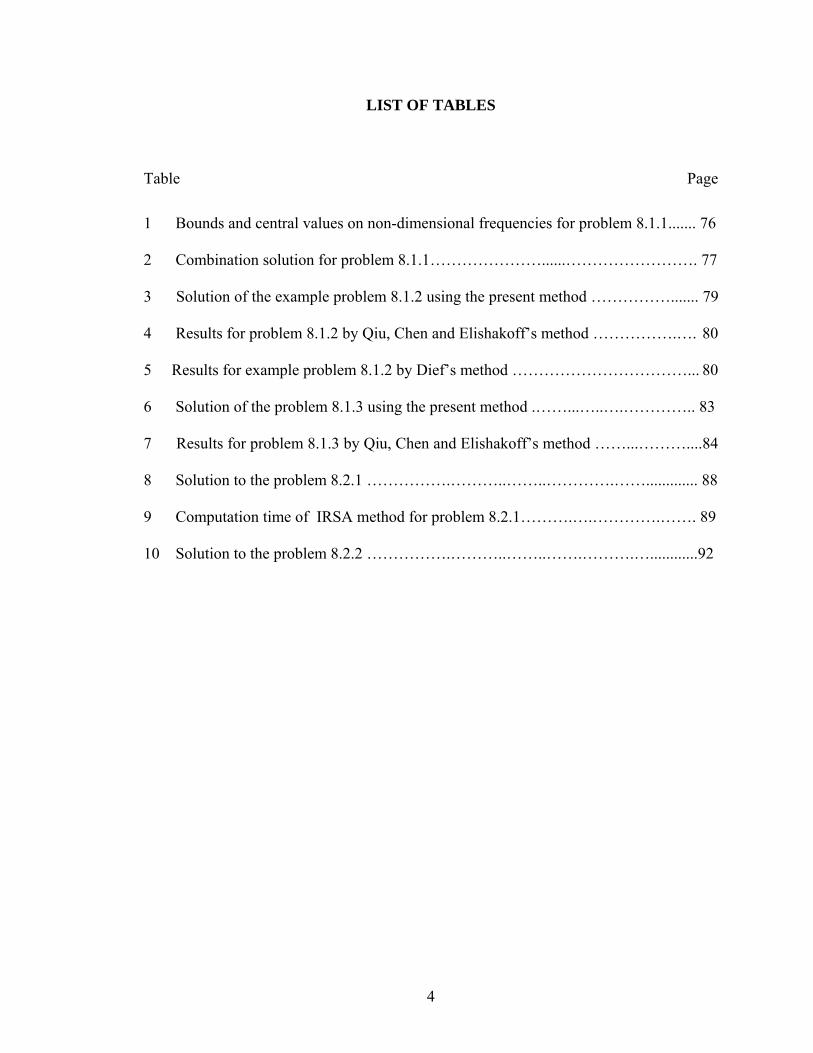
LIST OF TABLES

Table Page

1 Bounds and central values on non-dimensional frequencies for problem 8.1.1....... 76

2 Combination solution for problem 8.1.1…………………......……………………. 77

3 Solution of the example problem 8.1.2 using the present method ……………....... 79

4 Results for problem 8.1.2 by Qiu, Chen and Elishakoff’s method …………….…. 80

5 Results for example problem 8.1.2 by Dief’s method ……………………………... 80

6 Solution of the problem 8.1.3 using the present method .……...…..….………….. 83

7 Results for problem 8.1.3 by Qiu, Chen and Elishakoff’s method ……...………....84

8 Solution to the problem 8.2.1 …………….………..……..………….……............. 88

9 Computation time of IRSA method for problem 8.2.1……….….………….……. 89

10 Solution to the problem 8.2.2 …………….………..……..…….……….…............92

5

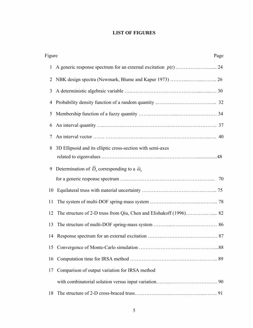
LIST OF FIGURES

Figure Page

1 A generic response spectrum for an external excitation )(tp …………………..... 24

2 NBK design spectra (Newmark, Blume and Kapur 1973) ………...……...……... 26

3 A deterministic algebraic variable …..…………………………………....…...…. 30

4 Probability density function of a random quantity ..……………………………... 32

5 Membership function of a fuzzy quantity …………………...…………………… 34

6 An interval quantity …..………………………………………………………….. 37

7 An interval vector ……. ………………….…………………………………...…. 40

8 3D Ellipsoid and its elliptic cross-section with semi-axes

related to eigenvalues .……………………………...………………….................48

9 Determination of nD~ corresponding to a nω~

for a generic response spectrum ….……………………………………………... 70

10 Equilateral truss with material uncertainty ……………………………….……... 75

11 The system of multi-DOF spring-mass system ………….…………….….……... 78

12 The structure of 2-D truss from Qiu, Chen and Elishakoff (1996)………….….... 82

13 The structure of multi-DOF spring-mass system ………...……………………… 86

14 Response spectrum for an external excitation …………………………………… 87

15 Convergence of Monte-Carlo simulation ………………………………………....88

16 Computation time for IRSA method …………………………………………….. 89

17 Comparison of output variation for IRSA method

with combinatorial solution versus input variation……...……………………….. 90

18 The structure of 2-D cross-braced truss………….………………………...…….. 91

6

ACKNOWLEDGEMENTS

The author expresses his deep and sincere gratitude to his academic advisor Prof.

Robert L. Mullen for the perceptive instructions and support as well as motivation and

encouragement that has inspired and nourished the author in numerous ways.

The author offers his deep appreciation to Prof. Dario A. Gasparini for the

constant help, substantial guidance, and insightful suggestions.

The author is grateful to Prof. Daniela Calvetti, Prof. Arthur A. Huckelbridge, and

Prof. Paul X. Bellini for providing their influential assistance.

7

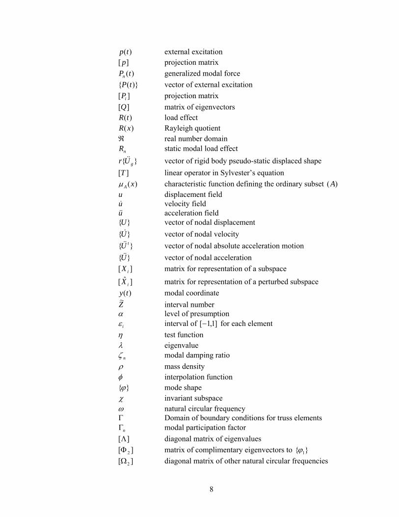
LIST OF SYMBOLS

A cross-sectional area A ordinary subset ][A symmetric matrix

]ˆ[A perturbed symmetric matrix αA interval of confidence of )(α cut c viscous damping ][C global damping matrix nD scaled modal coordinate E modulus of elasticity E referential set ][E perturbation matrix )(xf probability density function )(aFx cumulative probability function H Hilbert space i imaginary number )1( − ][I identity matrix nK generalized modal stiffness ][K global stiffness matrix ][K deterministic element stiffness contribution to the global stiffness matrix ]~[K interval global stiffness matrix ][ CK central stiffness matrix ][ eK stiffness matrix for a truss element ][ iK element stiffness matrix ]~[ RK radial stiffness matrix ][ iL element Boolean connectivity matrix ][L matrix representation of ][A on χ with respect to the basis ][X nM generalized modal mass ][M global mass matrix ][M deterministic element mass contribution to the global mass matrix ]~[M interval element mass matrix ][ eM mass matrix for a truss element ][ iM element mass matrix

8

)(tp external excitation ][ p projection matrix )(tPn generalized modal force )( tP vector of external excitation ][ iP projection matrix ][Q matrix of eigenvectors )(tR load effect )(xR Rayleigh quotient ℜ real number domain nR static modal load effect gUr && vector of rigid body pseudo-static displaced shape ][T linear operator in Sylvester’s equation )(xAµ characteristic function defining the ordinary subset )(A u displacement field u& velocity field u&& acceleration field U vector of nodal displacement U& vector of nodal velocity tU&& vector of nodal absolute acceleration motion U&& vector of nodal acceleration ][ iX matrix for representation of a subspace

]ˆ[ iX matrix for representation of a perturbed subspace )(ty modal coordinate Z~ interval number α level of presumption iε interval of ]1,1[− for each element η test function λ eigenvalue nζ modal damping ratio ρ mass density φ interpolation function ϕ mode shape χ invariant subspace ω natural circular frequency

Γ Domain of boundary conditions for truss elements nΓ modal participation factor ][Λ diagonal matrix of eigenvalues ][ 2Φ matrix of complimentary eigenvectors to 1ϕ ][ 2Ω diagonal matrix of other natural circular frequencies

9

Dynamic Analysis of Structures with Interval Uncertainty

Abstract

by

MEHDI MODARRESZADEH

A new method for dynamic response spectrum analysis of a structural system with

interval uncertainty is developed. This interval finite-element-based method is capable of

obtaining the bounds on dynamic response of a structure with interval uncertainty. The

proposed method is the first known method of dynamic response spectrum analysis of a

structure that allows for the presence of any physically allowable interval uncertainty in

the structure’s geometric or material characteristics and externally applied loads other

than Monte-Carlo simulation. The present method is performed using a set-theoretic

(interval) formulation to quantify the uncertainty present in the structure’s parameters

such as material properties. Independent variations for each element of the structure are

considered. At each stage of analysis, the existence of variation is considered as presence

of the perturbation in a pseudo-deterministic system. Having this consideration, first, a

linear interval eigenvalue problem is performed using the concept of monotonic behavior

of eigenvalues for symmetric matrices subjected to non-negative definite perturbation

which leads to a computationally efficient procedure to determine the bounds on a

structure’s natural frequencies. Then, using the procedures for perturbation of invariant

subspaces of matrices, the bounds on directional deviation (inclination) of each mode

shape are obtained.

10

Following this, the interval response spectrum analysis is performed considering

the effects of input variation in terms of the structure’s total response that includes

maximum modal coordinates, modal participation factors and mode shapes. Using this

method, it is shown that calculating the bounds on the dynamic response does not require

a combinatorial solution procedure. Several problems that illustrate the behavior of the

method and comparison with combinatorial and Monte-Carlo simulation results are

presented.

11

CHAPTER I

INTRODUCTION

1.1 Analytical Background

The dynamic analysis of a structure is an essential procedure to design a reliable

structure subjected to dynamic loads such as earthquake excitations. The objective of

dynamic analysis is to determine the structure’s response and interpret those theoretical

results in order to design the structure. Dynamic response spectrum analysis is one of the

methods of dynamic analysis which predicts the structure’s response using the

combination of modal maxima.

However, throughout conventional dynamic response spectrum analysis, the

possible existence of any uncertainty present in the structure’s geometric and/or material

characteristics is not considered. In the design process, the presence of uncertainty is

accounted for by considering a combination of load amplification and strength reduction

factors that are obtained by modeling of historic data. However, the impact of presence of

uncertainty on a design is not considered in the current deterministic dynamic response

spectrum analysis. In the presence of uncertainty in the geometric and/or material

properties of the system, an uncertainty analysis must be performed to obtain bounds on

the structure’s response.

12

Uncertainty analysis on the dynamics of a structure requires two major

considerations: first, modifications on the representation of the characteristics due to the

existence of uncertainty and second, development of schemes that are capable of

considering the presence of uncertainty throughout the solution process. Those developed

schemes must be consistent with the system’s physical behavior and also be

computationally feasible.

The set-theoretic (unknown but bounded) or interval representation of vagueness

is one possible method to quantify the uncertainty present in a physical system. The

interval representation of uncertainty in the parametric space has been motivated by the

lack of detailed probabilistic information on possible distributions of parameters and/or

computational issues in obtaining solutions.

In this work, a new method for dynamic response spectrum analysis of a structural

system with interval uncertainty entitled Interval Response Spectrum Analysis (IRSA) is

developed. IRSA enhances the deterministic dynamic response spectrum analysis by

including the presence of uncertainty at each step of the analysis procedure. In this finite-

element-based method, uncertainty in the elements is viewed by a closed set-

representation of element parameters that can vary within intervals defined by extreme

values. This representation transforms the point values in the deterministic system to

inclusive sets of values in the system with interval uncertainty.

The concepts of matrix perturbation theories are used in order to find the bounds

on the intervals of the terms involved in the modal contributions to the total structure’s

response including: circular natural frequencies, mode shapes and modal coordinates.

13

Having the bounds on those terms, the bounds on the total response are obtained

using interval calculations. Functional dependency and independency of intervals of

uncertainty are considered in order to attain sharper results. The IRSA can calculate the

bounds on the dynamic response without combinatorial or Monte-Carlo simulation

procedures. This computational efficiency makes IRSA an attractive method to introduce

uncertainty into dynamic analysis.

This work represents the synthesis of two historically independent fields,

structural dynamics and interval analysis. In order to represent the background for this

work, a review of development of both fields is presented.

1.2 Dissertation Overview

In chapter II, the analytical procedure for deterministic dynamic analysis is

presented. Chapter III is devoted to fundamentals of uncertainty analyses with emphasis

on the interval method. In chapter IV, matrix perturbation theories for eigenvalues and

eigenvectors are discussed. Chapter V introduces the method of interval response

spectrum analysis. In chapter VI, the bounds on variations of natural frequencies and

mode shapes are obtained. Chapter VII is devoted to determination of the bounds on the

total response of the structure. In chapter VIII, exemplars and numerical results are

presented. Chapter IX is devoted to observations and conclusions.

14

CHAPTER II

CONVENTIONAL DETERMINISTIC DYNAMIC ANALYSIS

2.1 Structural Dynamics Historical Background

Modern theories of structural dynamics were introduced mostly in mid 20th

century. M. A. Biot (1932) introduced the concept of earthquake response spectra and G.

W. Housner (1941) was instrumental in the widespread acceptance of this concept as a

practical means of characterizing ground motions and their effects on structures. N. M.

Newmark (1952) introduced computational methods for structural dynamics and

earthquake engineering. In 1959, he developed a family of time-stepping methods based

on variation of acceleration over a time-step.

A. W. Anderson (1952) developed methods for considering the effects of lateral

forces on structures induced by earthquake and wind and C. T. Looney (1954) studied

the behavior of structures subjected to forced vibrations. Also, D. E. Hudson (1956)

developed techniques for response spectrum analysis in engineering seismology. A.

Veletsos (1957) determined natural frequencies of continuous flexural members.

Moreover, he investigated the deformation of non-linear systems due to dynamic loads.

E. Rosenblueth (1959) introduced methods for combining modal responses and

characterizing earthquake analysis.

15

J. Biggs (1964) developed dynamic analyses for structures subjected to blast

loads. Moreover, numerical methods for dynamics of structures and modal analysis were

further developed by J. Penzien and R. W. Clough (1993).

2.2 Equation of Motion

In the development of IRSA, the truss element is used as the exemplar for a more

general finite element analysis. Other than the details of interval parameterization of the

resulting element matrices, the proposed method of IRSA should extend to a general

finite element analysis.

Considering the partial differential equation of motion for a truss element:

0)()( ,, =+−− tpuucEAu xx &&& ρ (2.1)

with B.C. : 2,1 , Γ=Γ= onpEAuongu x

in which, E is the modulus of elasticity, A is the cross-sectional area, c is the viscous

damping, ρ is the mass density and )(tp is the external excitation. The terms uu &, and

u&& are the displacement field and its temporal derivatives, respectively; and, x is the

spatial variable.

Multiplying by a test function )(η in spatial domain in order to find

)( 02og HHu ∈∀∈ η , in which H is the Hilbert space, Eq. (2.1) becomes:

0..)]()[( ,, =++−−∫

Ω

CBdxdttpuucEAu xx &&& ρη (2.2)

16

Integrating by parts to obtain the symmetric weak form to find )( 11og HHu ∈∀∈ η

yields:

0..)]([ ,, =+−++∫

Ω

CBdxdttpuucEAu xx ηηρηη &&& (2.3)

The spatial domain of displacement field and the test function can be semi-

discretized by approximating the functions u and η in space over each element by linear

interpolation functions as:

∑=I

II tuxtxu )()(),( φ (2.4)

∑=

III txtx )()(),( ηφη (2.5)

in which:

⎭⎬⎫

⎩⎨⎧ −

=Lx

LxLx T)(φ (2.6)

Substituting the above relationships over the elements yields:

(

) 0..)(][][][

...][][][][

,, =+Ω−

++∑ ∫Ω

CBdtpLULEAL

ULcLULL

TTxx

T

Element

TTTT

φφφ

φφφρφ &&&

(2.7)

where, U is the vector of nodal displacement, U& is the vector of nodal velocity, U&&

is the vector of nodal acceleration, the vector )( tP is the nodal external excitation and

[ L ] is the Boolean connectivity matrix.

17

Integrating over the domain, the equation of motion for vibration of a multiple

degree of freedom (DOF) system is defined as a linear system of ordinary differential

equations as:

)(][][][ tPUKUCUM =++ &&& (2.8)

where, ][ nnM × , ][ nnC × , and ][ nnK × are the global mass, global damping and global

stiffness matrices, respectively.

Stiffness and Mass Matrices for a Truss Element

The stiffness, consistent mass and lumped mass matrices for a linear truss element

are as following, respectively.

⎥⎦

⎤⎢⎣

⎡+−−+

=1111

][L

EAKe ⎥⎦

⎤⎢⎣

⎡=

2112

6][ ALM C

eρ ⎥

⎦

⎤⎢⎣

⎡=

1001

2][ ALM L

eρ

Solution to Equation of Motion

The solution of Eq.(2.8) can be divided into homogenous and particular parts. In

fact, the homogenous part is the solution to the free vibration of the system and the

particular part is the solution to the system’s forced vibration. Thus, in order to obtain the

solution to Eq.(2.8), the following procedure can be used.

18

2.3 Free Vibration

The equilibrium equations for the free vibration of an undamped multiple degree

of freedom system are defined as a set of linear homogeneous second-order ordinary

differential equations as:

0][][ =+ UKUM && (2.9)

Assuming a harmonic motion for the temporal displacement ( tieU ωϕ = ), Eq.(2.9) is

transformed to a set of linear homogeneous algebraic equations as:

0]))[(]([ 2 =− ϕω MK (2.10)

or: ])[(][ 2 ϕωϕ MK = (2.11)

Eq.(2.10) is known as a generalized eigenvalue problem between the stiffness and mass

matrices of the system.

The values of (ω ) are the natural circular frequencies and the vectors ϕ are the

corresponding mode shapes.

Solution to Eigenvalue Problem

For non-trivial solutions, the determinant of ]))[(]([ 2 MK ω− must be zero. This leads to

a scalar equation, known as the characteristic equation, whose roots are the system’s

natural circular frequencies of the system (ω ).

19

Substituting each value of circular frequency in Eq.(2.10) yields a corresponding

eigenvector or mode shape that is defined to an arbitrary multiplicative constant. The

modal matrix [ ]... 1 Nϕϕ spans the N-dimensional linear vector space.

This means that the eigenvectors ... 1 Nϕϕ form a complete basis, i.e., any

vector such as the vector of dynamic response of a multiple degree of freedom (MDOF)

system, )( tU , can be expressed as a linear combination of the mode shapes:

∑=

=+++=N

nnnNN tytytytytU

12211 )(.)(....)(.)(.)( ϕϕϕϕ (2.12)

in which, the terms )(tyn are modal coordinates and therefore, )( tU is defined in

modal coordinate space, since the values of ϕ are independent of time for linear

systems, Eq. (2.11).

Furthermore, the temporal derivatives of total response can be expressed as:

∑=

=+++=N

nnnNN tytytytytU

12211 )(.)(....)(.)(.)( &&&&& ϕϕϕϕ (2.13)

∑=

=+++=N

nnnNN tytytytytU

12211 )(.)(....)(.)(.)( &&&&&&&&&& ϕϕϕϕ (2.14)

which are also defined in modal coordinate space.

20

Orthogonality of Modes

Considering the generalized eigenvalue problem for the mth and nth circular

frequencies and corresponding mode shapes:

0]))[(]([ 2 =− mm MK ϕω (2.15)

0]))[(]([ 2 =− nn MK ϕω (2.16)

Pre-multiplying Eq.(2.15) and Eq.(2.16) by T

n ϕ and Tm ϕ , respectively:

0][)(][ 2 =− m

Tnmm

Tn MK ϕϕωϕϕ (2.17)

0][)(][ 2 =− nT

mnnT

m MK ϕϕωϕϕ (2.18)

Then, transposing Eq (2.18) and invoking the symmetric property of the ][K and ][M

matrices yields:

0][)(][ 2 =− mT

nnmT

n MK ϕϕωϕϕ (2.19)

Subtracting Eq.(2.19) from Eq.(2.17) yields:

( ) 0][)()( 22 =− m

Tnnm M ϕϕωω (2.20)

For any )( nm ≠ , if )( 22nm ωω ≠ :

0][ =mT

n M ϕϕ (2.21)

0][ =mT

n K ϕϕ (2.22)

Eqs.(2.21,2.22) express the characteristic of “orthogonality” of mode shapes with respect

to mass and stiffness matrices, respectively.

21

2.4 Forced Vibration

The equation of motion for forced vibration of an undamped MDOF system is

defined as:

)(][][ tPUKUM =+&& (2.23)

Expressing displacements and their time derivatives in modal coordinate space:

)()(][)(][11

tPtyKtyM n

N

nnn

N

nn =+∑∑

==

ϕϕ && (2.24)

Premultiplying each term in Eq.(2.24) by T

nϕ :

)()(][)(][11

tPtyKtyM Tnn

N

nn

Tn

N

nnn

Tn ϕϕϕϕϕ =+∑∑

==

&& (2.25)

Invoking orthogonality, Eq.(2.24) is reduced to a set of N uncoupled modal equations as:

)()(][)(][ tPtyKtyM T

nnnT

nnnT

n ϕϕϕϕϕ =+&& (2.26)

or: )()()( tPtyKtyM nnnnn =+&& (2.27)

where, ][,][ n

Tnnn

Tnn KKMM ϕϕϕϕ == and )()( tPtP T

nn ϕ= are generalized

modal mass, generalized modal stiffness and generalized modal force, respectively.

Dividing by modal mass nM and adding the assumed modal damping ratio ( nζ ),

Eq.(2.27) becomes:

n

nnnnnnn M

tPtytyty

)()()()()2()( 2 =++ ωωζ &&& (2.28)

22

Proportional Excitation

If loading is proportional )()( tpPtP = , meaning the applied forces have the

same time variation defined by )(tp (such as ground motion), Eq.(2.28) can be expressed

as:

( ))()()()()2()( 2 tpM

Ptytytyn

Tn

nnnnnnϕωωζ =++ &&& (2.29)

Defining a modal participation factor, nΓ , as:

][

nT

n

Tn

n

Tn

n MP

MP

ϕϕϕϕ

==Γ (2.30)

Also defining a scaled generalized modal coordinate:

n

nn

tytDΓ

=)()( (2.31)

Eq.(2.28) is rewritten in terms of the scaled modal coordinate ))(( tDn as:

)()()()()2()( 2 tptDtDtD nnnnnn =++ ωωζ &&& (2.32)

Therefore, using modal decomposition, the equation of motion for an N-DOF system is

uncoupled to N equations of motion of generalized single degree of freedom (SDOF)

systems.

23

2.4.1 Response History Analysis

In response history analysis (RHA), N uncoupled SDOF modal equations,

Eq.(2.32), are solved for the modal coordinates ))(( tDn , and then, by superposing the

modal responses, the total displacement response of the system is obtained as:

∑=

Γ=N

nnnn tDtU

1)))((()( ϕ (2.33)

in which the “time history” of the total response is obtained by the summation of modal

responses as products of time history of modal coordinates ))(( tDn , modal participation

factors )( nΓ , and modal displacements (mode shapes) nϕ . Moreover, the time history

of any load effect, )(tR , may be expressed as:

∑=

Γ=N

nnnn RtDtR

1

)))((()( (2.34)

in which, nR is a static modal load effect.

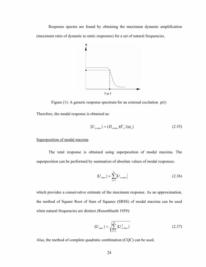
2.4.2 Response Spectrum Analysis

In response spectrum analysis (RSA), for each uncoupled generalized SDOF

modal equation, Eq.(2.32), the maximum modal coordinate )( max,nD is obtained using the

response spectrum of the external excitation )(tp and assumed modal damping nζ

(Figure(1)).

24

Response spectra are found by obtaining the maximum dynamic amplification

(maximum ratio of dynamic to static responses) for a set of natural frequencies.

Figure (1): A generic response spectrum for an external excitation )(tp

Therefore, the modal response is obtained as:

))(( max,max, nnnn DU ϕΓ= (2.35)

Superposition of modal maxima

The total response is obtained using superposition of modal maxima. The

superposition can be performed by summation of absolute values of modal responses.

∑=

=N

nnUU

1max,max (2.36)

which provides a conservative estimate of the maximum response. As an approximation,

the method of Square Root of Sum of Squares (SRSS) of modal maxima can be used

when natural frequencies are distinct (Rosenblueth 1959):

∑=

=N

nnUU

1

2max,max (2.37)

Also, the method of complete quadratic combination (CQC) can be used.

25

Ground Excitation- Response Spectrum Analysis

The equation of motion for an undamped MDOF system subjected to ground

excitation (support motion) from an earthquake is:

0][][ =+ UKUM t&& (2.38)

where tU&& is the vector of absolute acceleration. The vector U is defined as the

relative displacement vector, defined as:

)( g

t UrUU −= (2.39)

where gUr is the vector of rigid body pseudo-static displaced shape due to horizontal

ground motion. Substituting Eq.(2.39) in Eq.(2.38) yields:

gUrMUKUM &&&& ][][][ −=+ (2.40)

As before, solving the linear eigenvalue problem, defining the response in modal

coordinate space, uncoupling and adding assumed modal damping yields:

gn

Tn

Tn

nnnnnn UM

rMtytyty &&&&&

][][

)()()()2()( 2

ϕϕϕ

ωωζ −=++ (2.41)

Defining the modal participation factor, nΓ , as:

][

][

nT

n

Tn

n MrMϕϕ

ϕ=Γ (2.42)

26

Also, defining the scaled generalized modal coordinate nnn tytD Γ= /)()( , Eq.(2.40) may

be rewritten in terms of the scaled modal coordinate ))(( tDn as:

gnnnnnn UtDtDtD &&&&& −=++ )()()()2()( 2ωωζ (2.43)

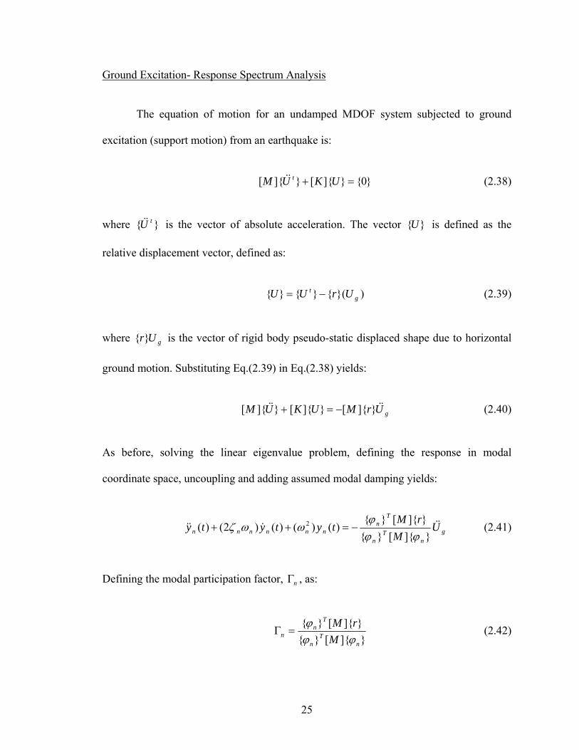
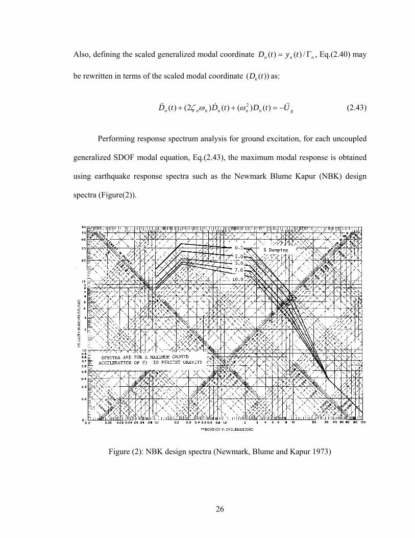
Performing response spectrum analysis for ground excitation, for each uncoupled

generalized SDOF modal equation, Eq.(2.43), the maximum modal response is obtained

using earthquake response spectra such as the Newmark Blume Kapur (NBK) design

spectra (Figure(2)).

Figure (2): NBK design spectra (Newmark, Blume and Kapur 1973)

27

Therefore, the maximum modal coordinate is obtained as:

),(max, nndn SD ζω= (2.44)

The total response is obtained using superposition of modal maxima. The superposition is

performed by considering Square Root of Sum of Squares (SRSS) of modal maxima:

∑=

Γ=N

nnnnDU

1

222max,max ϕ (2.45)

2.5 Response Spectrum Analysis Summary

Response spectrum analysis to compute the dynamic response of a MDOF to

external forces and ground excitation can be summarized as a sequence of steps as:

1. Define the structural properties.

• Determine the stiffness matrix ][K and mass matrix ][M .

• Assume the modal damping ratio nζ .

2. Perform a generalized eigenvalue problem between the stiffness and mass matrices.

• Determine natural circular frequencies ( nω ).

• Determine mode shapes nϕ .

28

3. Compute the maximum modal response.

• Determine the maximum modal coordinate max,nD using the excitation response

spectrum for the corresponding natural circular frequency and modal damping

ratio.

• Determine the modal participation factor nΓ .

• Compute the maximum modal response as a product of maximum modal

coordinate, modal participation factor and mode shape.

4. Combine the contributions of all maximum modal responses to determine the

maximum total reponse using SRSS or other combination methods.

Limitations

In the presence of uncertainty in the structure’s physical or geometrical

parameters, the deterministic structural dynamic analysis cannot be performed and hence,

a new method must be developed to incorporate an uncertainty analysis into the

conventional response spectrum analysis.

29

CHAPTER III

UNCERTAINTY ANALYSIS FUNDAMENTALS

3.1 Background

In structural engineering, design of an engineered system requires that the

performance of the system is guaranteed over its lifetime. However, the parameters for

designing a reliable structure possess physical and geometrical uncertainties. The

presence of uncertainty can be attributed to physical imperfections, model inaccuracies

and system complexities. Moreover, neither the initial conditions, nor external forces,

nor the constitutive parameters can be perfectly described. Therefore, in order to design a

reliable structure, the possible uncertainties in the system must be included in the analysis

procedures.

Categories of Uncertainty

The concept of uncertainty can be divided into two major categories:

• Aleatory: The system has an intrinsic random or stochastic nature and it is not

predictable.

• Epistemic: The uncertainty induced by the lack of knowledge and it is predictable.

30

Example of aleatory uncertainty is the behavior of photons in quantum mechanics

where there is no hidden variable in the model or missing information.

Epistemic systems have uncertainty that may be reduced upon additional

information. Uncertainty in the stiffness of a structural member may be reduced by

measurement of the element behavior.

Aleatory uncertainty assumes that an underlying probability density function

(PDF) exists and is the square of the wave function in quantum mechanics and also, the

PDF is a fundamental property of the system.

In most engineering systems, the PDF is obtained from historic data and

represents both epistemic and aleatory uncertainties. Thus, the precise form of a PDF can

only be assumed. On the other hand, interval methods play an important role in

quantifying epistemic uncertainty.

Deterministic analysis

In deterministic analysis of physical systems, defining the system’s characteristics

as point quantities, using conventional deterministic algebraic values, is sufficient to

model the system and perform the analysis (Figure(3)).

Figure (3): A deterministic algebraic variable

ax =

31

3.2 Uncertainty Analysis

In order to perform uncertainty analysis on a physical system, the uncertainty

present in the system’s physical characteristics must be fully mathematically quantified.

Presently, there are three paradigms to consider uncertainty in non-deterministic

structural analysis:

1. Stochastic analysis

In stochastic analysis, the theory of probability which was developed based on

aleatory uncertainty. Extensions have been made such as “degree of belief” probability

on subjective probability which includes epistemic effects.

2. Fuzzy analysis

In fuzzy analysis, the theory of possibility for fuzzy sets is used which assumes

epistemic uncertainty.

3. Interval analysis

In interval analysis, the theory of convex (interval) sets is used which assumes

epistemic or aleatory uncertainties (such as Dempster-Shafer bounds that are epistemic

bounds on aleatory probability functions).

32

3.3 Stochastic Analysis

The stochastic approach to uncertain problems is to model the structural

parameters as random quantities (Pascal 1654). Therefore, all information about the

structural parameters is provided by the probability density functions. This probability

density function is then used to determine an estimate of the system’s behavior.

Random Variable

A random quantity, used in stochastic analysis, is defined by a deterministic function that

yields the probability of existence of the random variable in a given subset of the real

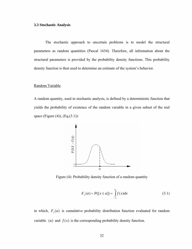
space (Figure (4)), (Eq.(3.1)):

Figure (4): Probability density function of a random quantity

∫∞−

=≤=a

x dxxfaxPaF )(])([)( (3.1)

in which, )(aFx is cumulative probability distribution function evaluated for random

variable )(a and )(xf is the corresponding probability density function.

33

3.4 Fuzzy Analysis

The fuzzy approach to the uncertain problems is to model the structural

parameters as fuzzy quantities (Lotfi-zadeh 1965). In conventional set theories, either an

element belongs or doesn’t belong to set. However, fuzzy sets have a membership

function that allows for “partial membership” in the set. Using this method, structural

parameters are quantified by fuzzy sets. Following fuzzifying the parameters, structural

analysis is performed using fuzzy operations.

Fuzzy Subset

Considering E as a referential set inℜ , an ordinary subset A of the referential set

is defined by its characteristic function )(xAµ as:

1,0)(: ∈∈∀ xEx Aµ (3.2)

which exhibits whether or not, an element of E belongs to the ordinary subset A. For the

same referential set E, a fuzzy subset A is defined by its characteristic function,

membership function )(xAµ , as:

]1,0[)(: ∈∈∀ xEx Aµ (3.3)

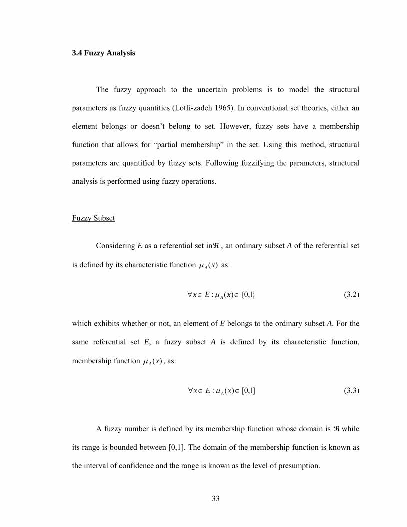
A fuzzy number is defined by its membership function whose domain is ℜwhile

its range is bounded between [0,1]. The domain of the membership function is known as

the interval of confidence and the range is known as the level of presumption.

34

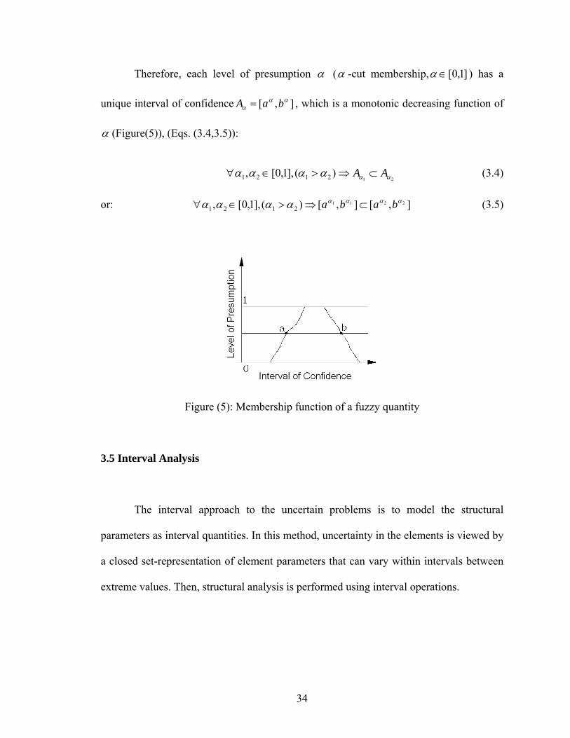
Therefore, each level of presumption α (α -cut membership, ]1,0[∈α ) has a

unique interval of confidence ],[ ααα baA = , which is a monotonic decreasing function of

α (Figure(5)), (Eqs. (3.4,3.5)):

21)(],1,0[, 2121 αααααα AA ⊂⇒>∈∀ (3.4)

or: ],[],[)(],1,0[, 22112121

αααααααα baba ⊂⇒>∈∀ (3.5)

Figure (5): Membership function of a fuzzy quantity

3.5 Interval Analysis

The interval approach to the uncertain problems is to model the structural

parameters as interval quantities. In this method, uncertainty in the elements is viewed by

a closed set-representation of element parameters that can vary within intervals between

extreme values. Then, structural analysis is performed using interval operations.

35

Interval Analysis Historical Background

The concept of representation of an imprecise real number by its bounds is quite

old. In fact, Archimedes (287-212 B.C.) defined the irrational number (π) by an interval

713

71103 << π , which he found by approximating the circle with the inscribed and

circumscribed 96-side regular polygons. Early work in modern interval analysis was

performed by W. H. Young (1908), who introduced functions with values which are

bounded between extreme limits. The concept of operations with a set of multi-valued

numbers was introduced by R. C. Young (1931), who developed a formal algebra of

multi-valued numbers. Also, the special case of multi-valued functions with closed

intervals was discussed by Dwyer (1951). The introduction of digital computers in the

1950’s provided impetus for further interval analysis as discrete representations of real

numbers with associated truncation error.

Interval mathematics was further developed by Sunaga (1958) who introduced the

theory of interval algebra and its applications in numerical analysis. Also, R. Moore

(1966) introduced interval analysis, interval vectors and interval matrices as a set of

techniques that provides error analyses for computational results.

Interval analysis provides a powerful set of tools with direct applicability to

important problems in scientific computing. Alefeld and Herzberger (1983) presented an

extensive treatment of interval linear and non-linear algebraic equations and interval

methods for systems of equations. Moreover, Neumaier (1990) investigated the methods

for solution of interval systems of equations.

36

The concept of interval systems has been further developed in analysis of

structures with interval uncertainty. Muhanna and Mullen (1999) developed fuzzy finite-

element methods for solid mechanics problems. For the solution of interval finite

element method (IFEM) problems, Muhanna and Mullen (2001) introduced an Element-

by-Element interval finite element formulation, in which a guaranteed enclosure for the

solution of interval linear systems of equations was achieved.

The research in interval eigenvalue problem began to emerge as its wide

applicability in science and engineering was realized. Dief (1991) presented a method for

computing interval eigenvalues of an interval matrix based on an assumption of

invariance properties of eigenvectors. Using Dief’s method, the lower eigenvalues have a

wider range of uncertainty than the exact results.

The concept of the interval eigenvalue problem has been developed in dynamics

of structures with uncertainty. Qiu, Chen and Elishokoff (1995) have introduced a

method to find the bounds on eigenvalues. In their work, the perturbation of the

eigenvalue is derived from pre and post multiplying the perturbed matrix by the exact

eigenvector which is inconsistent with matrix perturbation theories.

However, since the presence of perturbation in the matrix results in perturbation

of both eigenvalues and eigenvectors, applying the unperturbed eigenvector to determine

the perturbation of the eigenvalue may lead to incorrect results. The second problem in

this work solves the problem cited by Qiu, Chen and Elishokoff (1995) for exact bounds

with the present scheme and illustrates the difference in solution.

37

Qiu, Chen and Elishokoff (1996) have introduced an alternate method for

bounding the natural frequencies of a structural system. However, their results are wider

than sharp values because of a non-parametric formulation and the existence of variation

inside the matrices. Moreover, their definition of the concept of maximin characterization

appears to be inconsistent with the formal mathematical definitions. The constraint-

induced subspaces in this concept are not completely arbitrary but they should be

orthogonal to arbitrary vectors (Bellman 1960 and Strang 1976). The third problem in the

present work solves the problem cited by Qiu, Chen and Elishokoff (1996) with the

present scheme and compares the results.

As part of the present work, Modares and Mullen (2004) have introduced a

method for the solution of the parametric interval eigenvalue problem resulting from

semi-discretization of structural dynamics which determines the exact bounds of the

natural frequencies of a structure.

Interval (Convex) Number

A real interval is a closed set defined by extreme values as (Figure(6)):

|],[~ ulul zzzzzzZ ≤≤ℜ∈== (3.6)

Figure (6): An interval quantity

],[~ bax =

38

One interpretation of an interval number is a random variable whose probability

density function is unknown but non-zero only in the range of interval.

Another interpretation of an interval number includes intervals of confidence for

α -cuts of fuzzy sets. This interval representation transforms the point values in the

deterministic system to inclusive set values in the system with bounded uncertainty.

Interval Arithmetic Operations

Interval arithmetic is a computational tool that can be used to represent

uncertainty as:

1. A set of probability density functions.

2. In Dempster-Shafer models for epistemic probability.

3. α - cuts in fuzzy sets.

In this work, the symbol (~) represents an interval quantity. Considering

],[~ baX = and ],[~ dcY = as two interval numbers, the basic interval arithmetic

operations are:

Addition:

],[~~ dbcaYX ++=+ (3.7)

Subtraction:

],[~~ cbdaYX −−=− (3.8)

39

Multiplication by scalar:

]),,max(),,[min(~ babaX βββββ =× (3.9)

Multiplication:

)],,,max(),,,,[min(~~ bdbcadacbdbcadacYX =× (3.10)

Properties of Interval Multiplication:

Associative:

XYYX ~~~~ ×=× (3.11)

Commutative:

ZYXZYX ~)~~()~~(~ ××=×× (3.12)

Distributive:

ZXYXZYX ~~~~)~~(~ ×+×⊂+× (3.13)

Therefore, the distributive property of interval multiplication is weaker than that

in conventional algebra and it is one possible cause of loss of sharpness in interval

operations.

40

Division:

]),[0(],1,1[],[~~

dccd

baYX

∉×= (3.14)

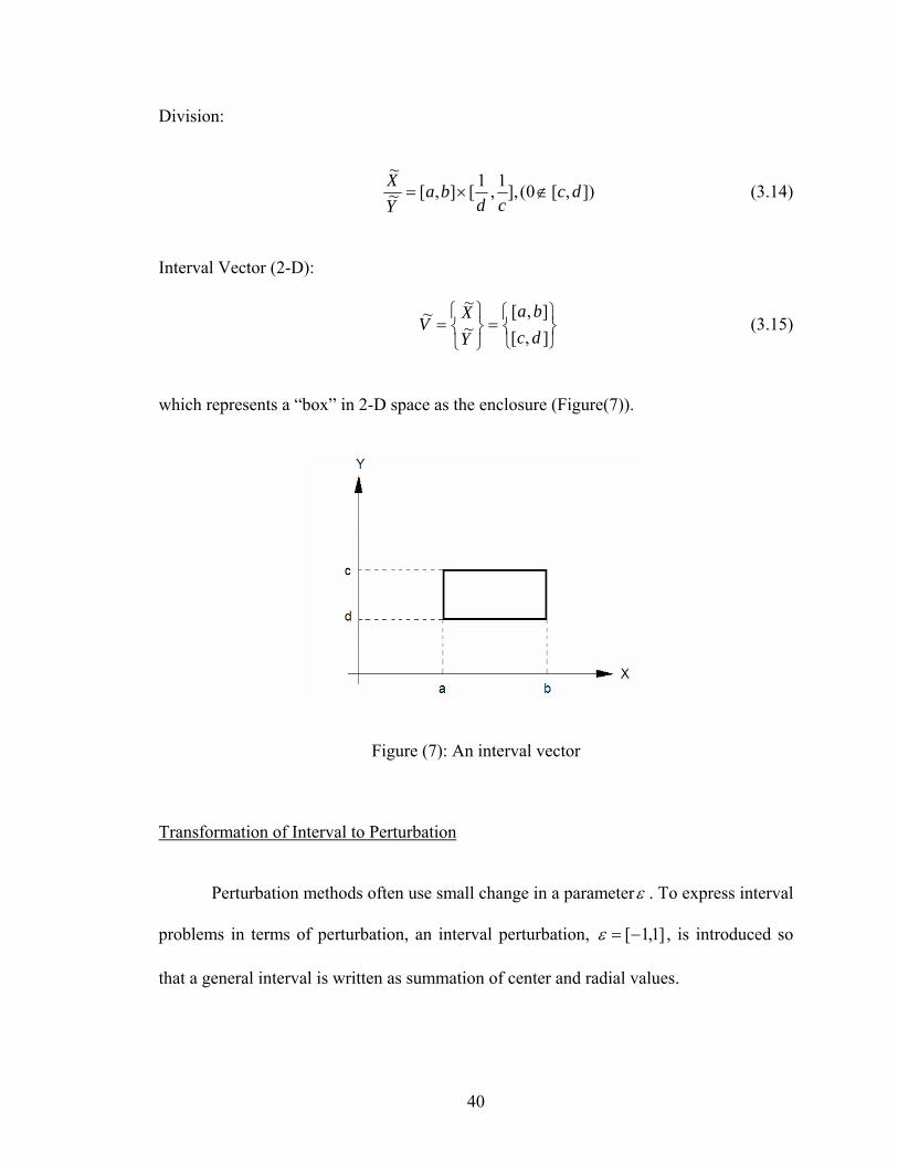
Interval Vector (2-D):

⎭⎬⎫

⎩⎨⎧

=⎭⎬⎫

⎩⎨⎧

=],[],[

~~

~dcba

YX

V (3.15)

which represents a “box” in 2-D space as the enclosure (Figure(7)).

Figure (7): An interval vector

Transformation of Interval to Perturbation

Perturbation methods often use small change in a parameterε . To express interval

problems in terms of perturbation, an interval perturbation, ]1,1[−=ε , is introduced so

that a general interval is written as summation of center and radial values.

41

Considering ],[~ ulZ = as an interval number, the median and radius can be

defined as:

)2

( ulZ C+

= (3.16)

)2

)((~ luZ R−

= ε (3.17)

So, Z~ can be redefined as:

RC ZZZ ~~ += (3.18)

where, the interval number is shown as its median subjected to a perturbation of radius by

which, the result encompasses the range of the interval between the extreme values.

Functional Dependency of Interval Operations

Considering ]2,2[~ −=X and ]2,2[~ −=Y as two independent interval numbers, the

functional dependent interval multiplication results in:

]4,0[~~ =× XX

In contrast, the functional independent interval multiplication results in:

]4,4[~~ −=×YX

42

Sharpness Considerations in Engineering

In interval operations, the functional dependency of intervals must be considered

in order to attain sharper results. In fact, the issue of sharpness and overestimation in

interval bounds is the key limitation in the application of interval methods. Naïve

implementation of interval arithmetic algorithms (substituting interval operations for their

scalar equivalence) will yield bounds that are not useful for engineering design.

Therefore, there is a need to develop algorithms to calculate sharp or nearly sharp bounds

to the underlying set theoretic interval problems.

For instance, the calculation of exact sharp bounds to the interval system of

equations resulting from linear static analysis using the finite element method has been

proved to be computationally combinatorial problem. However, even the 2n combinations

of upper and lower bounds do not always yield the bounds.

In problems with narrow intervals associated with truncation errors, the naïve

implementation of interval arithmetic will yield acceptable bounds. However, for wider

intervals representing uncertainty in parameters, the naïve method will overestimate the

bounds by several orders of magnitude.

Successful applications of the interval method in the linear static problem have

required the development of new algorithms that are computationally feasible yet still

provide nearly sharp bounds (Muhanna and Mullen 2003).

43

Objective

The goal of this research is to solve an interval structural dynamics problem, i.e.,

given uncertainty in material or geometric properties expressed as intervals multiplying

element stiffness or mass matrices, find the interval bounds on the structure’s response.

One approach for solution to the interval system is applying perturbation theories

of mathematics to the interval system. Specifically, perturbation theories in eigenvalue

problems, needed for structural dynamics, can be used to obtain the bounds on

eigenvalues and eigenvectors that will be addressed in the next chapter. However, some

perturbation theories require the constraint of smallness of the radial perturbation in

comparison with the median value. This smallness must be considered throughout the

analysis procedure.

44

CHAPTER IV

MATRIX PERTURBATION THEORIES

4.1 Perturbation of Eigenvalues

The classical linear eigenvalue problem for a symmetric matrix ( TAA ][][ = ) is:

][ xxA λ= (4.1)

with the solution of real eigenvalues ( nλλλ ≤≤≤ ...21 ) and corresponding eigenvectors

( nxxx ,...,, 21 ). This equation can be transformed into a ratio of quadratics known as the

Rayleigh quotient:

][)(xx

xAxxR T

T

= (4.2)

Transforming the Rayleigh quotient to the principal basis with the orthogonal matrix ][Q

(matrix of eigenvectors) obtained by the eigenvalue decomposition of matrix

( TQQA ]][][[][ Λ= ), in which ][Λ is the diagonal matrix of eigenvalues and

( ][ xQy T= ), the quotient becomes:

221

2222

211

......

][

)]([)]([)]]([[)]([)(

n

nnT

T

T

T

yyyyy

yyyy

yQyQyQAyQxR

+++++

=Λ

==λλλ (4.3)

45

Furthermore:

1221

2

1

22

1

2211

...

)...()( λ

λλ

λλ

λ≥

++

+++=

n

nn

yy

yyyxR (4.4)

nn

nnn

n

yy

yyyxR λ

λλ

λλ

λ≤

++

+++= 22

1

222

221

1

...

)...()( (4.5)

Therefore, the Rayleigh quotient for a symmetric matrix is bounded between the smallest

and the largest eigenvalues (Strang 1976).

nT

T

xxxAxxR λλ ≤=≤

][)(1 (4.6)

Thus, the first eigenvalue ( 1λ ) can be obtained by performing an unconstrained

minimization on the scalar-valued function of Rayleigh quotient:

1)

][(min)(min λ==∈∈ xx

xAxxR T

T

RxRx nn (4.7)

In order to find the intermediate eigenvalues, additional constraints must be

imposed on this minimization problem. The second eigenvalue can be determined by

imposing a single constraint, i.e., the trial vector x shall be perpendicular to an

arbitrary vector z )0( =zx T .This restriction changes the problem to a set of

constrained minimizations whose upper-bound is the second smallest eigenvalue ( 2λ ). So

for any choice of z :

210

)()(min λµ ≤==

zxRzxT

(4.8)

46

This is proven by considering the trial vector x as a non-zero combination of

the first and second normalized eigenvectors:

21 xxx βα += (4.9)

in which, x will be orthogonal to z . This only imposes a single condition on (α ) and

( β ). For any combination of the first two eigenvectors:

222

22

21

2121

2121

)()()]([)(

)( λβαβλαλ

βαβαβαβα

≤++

=++++

=xxxx

xxAxxxR T

T

(4.10)

Therefore, the minimization of )(xR subject to a single constraint )0( =zx T

and then choosing the vector z that maximizes these minima yields the second smallest

eigenvalue ( 2λ ).

)](minmax[

02 xR

zxT ==λ (4.11)

This result can be generalized to obtain the next eigenvalues by applying

additional constraints to )(xR as:

)](max[min xRk =λ (4.12)

(subject to constrains 2,1,...1),0( ≥−== kkizx iT )

This principle is called the maximin characterization of eigenvalues for symmetric

matrices.

47

Geometric Observation

Geometrically, if [A] is positive definite, the numerator of the Rayleigh quotient

( 1][ =xAx T ) defines a hyper-ellipsoid in n-dimensional space which is centered at

the origin. Transforming the system to the principal basis, the equation of the hyper-

ellipsoid is:

1... 22

22211 =+++ nn yyy λλλ (4.13)

Therefore, the principal axes of the hyper-ellipsoid are in the directions of the

eigenvectors. Furthermore, pointing to the direction of the jth eigenvector

)](),0[( jiyi ≠= :

j

jjj yyλ

λ 112 =→= (4.14)

Thus the length of each semi-axis is the reciprocal of the square root of the

eigenvalue whose corresponding eigenvector is collinear with that semi-axis (Strang

1976). Therefore, performing the unconstrained minimization on the Rayleigh quotient,

which finds the absolute minimum ( 1λ ), can geometrically be interpreted as determining

the semi-axis of greatest length )/1( 11 λ=y .

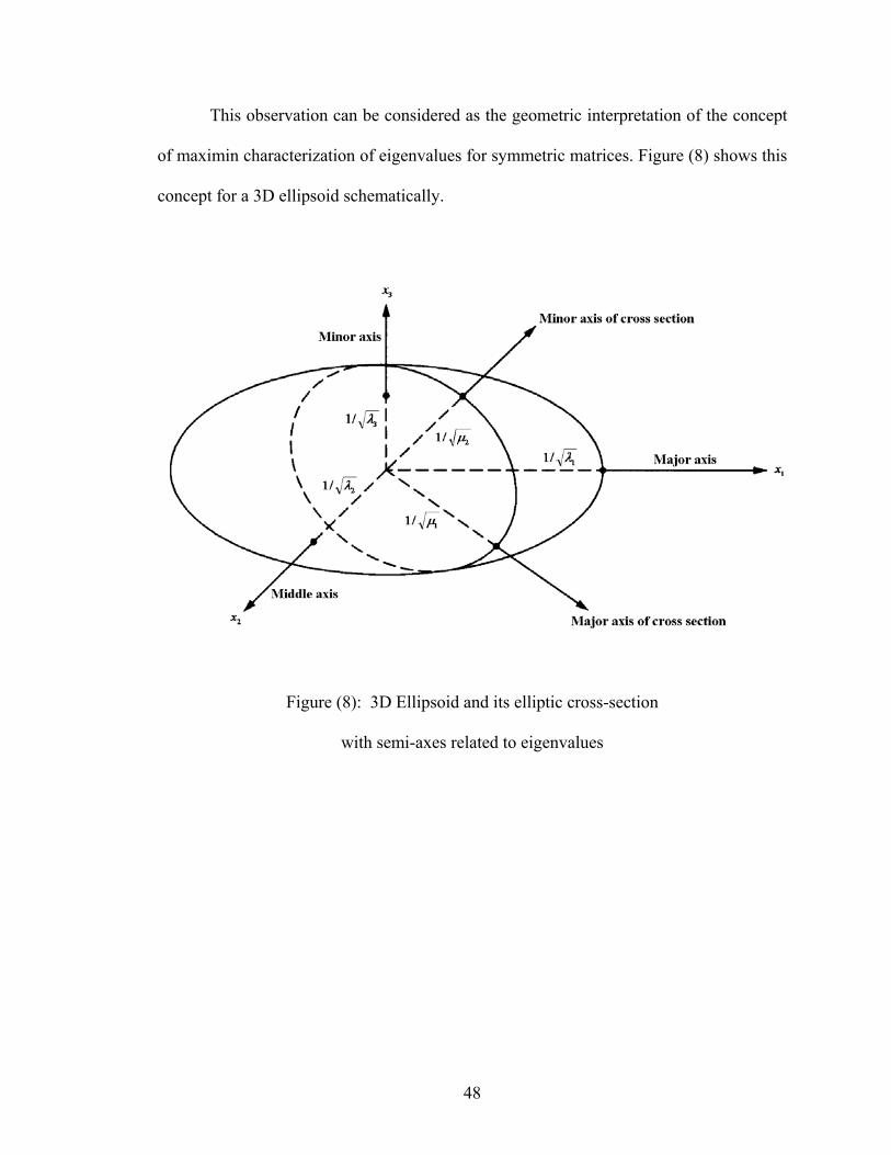
Passing an arbitrary plane through the origin of hyper-ellipsoid creates a cross-

section which is again an ellipsoid, in one lower dimension. If this cross-sectional

ellipsoid is rotated until its greatest semi-axis )/1( 1µ assumes its smallest value, the

semi-axis of the original ellipsoid of second greatest length is determined )/1( 22 λ=y .

48

This observation can be considered as the geometric interpretation of the concept

of maximin characterization of eigenvalues for symmetric matrices. Figure (8) shows this

concept for a 3D ellipsoid schematically.

Figure (8): 3D Ellipsoid and its elliptic cross-section

with semi-axes related to eigenvalues

49

Symmetric Matrix Non-Negative Definite Perturbation

If the symmetric matrix [A] is subjected to a symmetric non-negative definite

perturbation matrix ][E , )0][( ≥xEx T using the unconstrained minimization of

)(xR , the first eigenvalue of the perturbed matrix is:

)(

][min

][min)(ˆ11 A

xxxAx

xxxEAxEA T

T

T

T

λλ =≥+

=+ (4.15)

For the next eigenvalues of the perturbed matrix, the maximin characterization of

eigenvalues can be used as:

)(]

][minmax[]

][minmax[)(ˆ1,...,1,01,...,1,0

Axx

xAxxx

xEAxEA kT

T

kizxT

T

kizxk

iT

iT

λλ =≥+

=+−==−==

(4.16)

Therefore, all eigenvalues of a symmetric matrix subject to a non-negative

definite perturbation monotonically increase from the eigenvalues of the exact matrix.

)()(ˆ AEA kk λλ ≥+ (4.17)

Similarly, all eigenvalues of a symmetric matrix subject to a non-positive definite

perturbation monotonically decrease from the eigenvalues of the exact matrix.

)()(ˆ AEA kk λλ ≤− (4.18)

50

This concept is known as the “monotonic behavior” of eigenvalues of symmetric matrices

subject to a symmetric non-negative (or non-positive) perturbation (Bellman 1960).

4.2 Perturbation of Eigenvectors

4.2.1 Theory of Simple Invariant Subspaces

Invariant Subspace

The subspace χ is defined to be an invariant subspace of matrix ][A if:

χχ ⊂A (4.19)

This means that if χ is an invariant subspace of nnA ×][ and also, columns of mnX ×][ 1

form a basis for χ , then there is a unique matrix mmL ×][ 1 such that:

]][[]][[ 111 LXXA = (4.20)

The matrix ][ 1L is the representation of ][A on χ with respect to the basis ][ 1X

and the eigenvalues of ][ 1L are a subset of eigenvalues of ][A . Therefore, for the

invariant subspace, ),( λv is an eigenpair of ][ 1L if and only if ),]([ 1 λvX is an

eigenpair of ][A .

51

Theorem of Invariant Subspaces

For a real symmetric matrix ][A , considering the subspace χ with the linearly

independent columns of ][ 1X forming a basis for χ and the linearly independent

columns of ][ 2X spanning the complementary subspace ⊥χ , then, χ is an invariant

subspace of ][A if and only if:

]0[]][[][ 12 =XAX T (4.21)

Therefore, invoking the necessary and sufficient condition and postulating the

definition of invariant subspaces, the symmetric matrix ][A can be reduced to a

diagonalized form using a unitary similarity transformation as:

⎥⎦

⎤⎢⎣

⎡=⎥

⎦

⎤⎢⎣

⎡=

][]0[]0[][

]][[][]][[][]][[][]][[][

]][[][2

1

2212

21112121 L

LXAXXAXXAXXAX

XXAXX TT

TTT (4.22)

where .2,1],][[][][ == iXAXL iT

ii

Simple Invariant Subspace

An invariant subspace is simple if the eigenvalues of its representation ][ 1L are

distinct from other eigenvalues of ][A . Thus, using the reduced form of ][A with respect

to the unitary matrix ]]][[[ 21 XX , χ is a simple invariant subspace if the eigenvalues of

][ 1L and ][ 2L are distinct:

∅=])([])([ 21 LL λλ I (4.23)

52

Spectral Resolution

The symmetric matrix ][A can be decomposed as the summation of contributions

of simple invariant subspaces χ and ⊥χ as:

TT XLXXLXA ]][][[]][][[][ 222111 += (4.24)

which is the spectral resolution of the matrix ][A into two complementary invariant

subspaces.

Spectral Projection

Considering the projection matrices 2,1,]][[][ == iXXP T

iii with properties as:

)2,1(][][ 2 == iPP ii (4.25a)

]0[]][[]][[ 1221 == PPPP (4.25b)

]][][[]][][[][ 2211 PAPPAPA += (4.25c)

hence, any vector z can be decomposed into the sum of two vectors, 21 xxz +=

and ( ⊥∈∈ χχ , 21 xx ), in which, the decomposed component vectors are obtained

using projection matrices as:

][ 11 zPx = (4.26)

][])[]([ 212 zPzPIx =−= (4.27)

which are known as spectral projections of simple invariant subspaces.

53

4.2.2 Perturbation of Simple Invariant Subspaces

Considering the column spaces of ][ 1X and ][ 2X to span two complementary

simple invariant subspaces, the perturbed orthogonal subspaces are defined as:

]][[][]ˆ[ 211 PXXX += (4.28)

TPXXX ]][[][]ˆ[ 122 −= (4.29)

in which ][P is a matrix to be determined. Thus, each perturbed subspace is defined as a

summation of the exact subspace and the contribution of the complementary subspace.

Orthonormalization:

Performing inner products on each perturbed subspace, Eqs(4.28,4.29), as:

])[][]([]ˆ[]ˆ[ 11 PPIXX TT += (4.30)

)]][[]([]ˆ[]ˆ[ 22TT PPIXX += (4.31)

the perturbed complementary subspaces can be orthonormalized as:

21

211 ])[][]])([][[]([]ˆ[−

++= PPIPXXX T (4.32)

21

122 )]][[])([]][[]([]ˆ[−

+−= TT PPIPXXX (4.33)

in which, the redefined perturbed subspaces have orthonormal columns.

54

Perturbation Problem

Considering a symmetric perturbation ][E , the perturbed matrix is defined as:

][][]ˆ[ EAA += (4.34)

Performing the similarity transformation on the symmetric perturbed matrix ]~[A using

the unitary matrix ]]ˆ][ˆ[[ 21 XX obtained from the orthonormalized perturbed subspaces as:

⎥⎦

⎤⎢⎣

⎡=

]ˆ[]ˆ[]ˆ[]ˆ[]ˆˆ][ˆ[]ˆˆ[2

12121 LG

GLXXAXXT

T (4.35)

Then, using the theorem of invariant subspaces, ]ˆ[ 1X is an invariant subspace if and only

if:

]0[]ˆ][ˆ[]ˆ[]ˆ[ 12 == XAXG T (4.36)

Substituting the perturbed matrix and perturbed subspaces, Eqs.(4.32-4.34), and

linearizing the result due to a small perturbation compared to the unperturbed matrix,

Eq(4.36) is rewritten as:

]][[][]][[]][[ 1221 XEXPLLP T=− (4.37)

This perturbation problem is an equation for unknown ][P in the form of a Sylvester’s

equation.

55

Sylvester’s Equation

A Sylvester’s equation (J. J. Sylvester 1814-1897) is of the form:

][]][[]][[ CBXXA =− (4.38)

in which, nnA ×][ , mmB ×][ and mnC ×][ are known matrices, and mnX ×][ is the unknown

matrix to be determined. Equivalently, a linear operator ][T can be defined as:

mnmn BXXAXT ×× −→= ])][[]][([][][ (4.39)

The uniqueness of the solution to the Sylvester’s equation is guaranteed when the

operator ][T is nonsingular. The operator ][T is nonsingular if and only if the

eigenvalues of ][A and ][B are distinct:

∅=])([])([ BA λλ I (4.40)

Thus, for the perturbation problem, Eq.(4.37), the uniqueness of the solution matrix ][P

is guaranteed if the eigenvalues of ][ 1L and ][ 2L are distinct and hence, for the

uniqueness, the column spaces of ][ 1X and ][ 2X must span two simple invariant

subspaces, Eq.(4.23).

56

4.2.3 Perturbation of Eigenvectors

The perturbation of the first eigenvector, using Eq.(4.28), is defined as:

]][[ˆ 211 pXxx += (4.41)

Thus, the perturbation problem, Eq.(4.37), is considerably simplified as:

][][]][[][ 1221 xEXpLp T=−λ (4.42)

since, the operator ][T is specialized as ])[][( 21 LI −λ . If )( 1λ is a simple eigenvalue, the

solution for ][ p exists and is unique as:

][][])[][(][ 12

121 xEXLIp T−−= λ (4.43)

Therefore the perturbed eigenvector is:

][][])[][]([ˆ 12

121211 xEXLIXxx T−−+= λ (4.44)

Also, the number TXLIX ][])[][]([ 2

1212

−−λ is known as the condition number of the

eigenvector 1x (Stewart and Guang 1991).

For each eigenvalue, the perturbed eigenvector can be found using Eq. (4.44).

57

CHAPTER V

INTERVAL RESPONSE SPECTRUM ANALYSIS

As mentioned in chapter II, in the presence of uncertainty in the structure’s

geometrical or material characteristics, the conventional response spectrum analysis

cannot be performed to obtain the structure’s responses. In this work, a new method is

developed which is capable of performing a response spectrum analysis and obtaining the

bounds on the structure’s response when the parameters in the structure are unknown but

bounded. This method, entitled Interval Response Spectrum Analysis (IRSA), enhances

the procedure in deterministic response spectrum analysis to take into account the

existence of interval uncertainty throughout the solution process.

5.1 IRSA Procedure:

First, IRSA defines the uncertainty in the system’s parameters as closed intervals,

therefore, the imprecise property can vary within the intervals between extreme values

(bounds). Then, having the uncertain parameters represented by interval variables for

each element, the interval global stiffness and mass matrices of MDOF system are

assembled. This assemblage is performed such that the element physical characteristics

and the matrix mathematical properties are preserved.

58

Then an interval generalized eigenvalue problem between the interval stiffness

and mass matrices is established. From this interval eigenvalue problem, two solutions of

interest are obtained:

1. Bounds on variation of circular natural frequencies (Interval natural frequencies)

2. Bounds on directional deviation of mode shapes (Interval mode shapes)

Then, the interval modal coordinate and the maximum modal coordinate are

determined using the excitation response spectrum evaluated for the corresponding

interval of natural circular frequency and assumed modal damping ratio. Then, the

interval modal participation factor is computed. Dependency or independency of

variations in interval modal participation factor is considered. Following this, the

maximum modal response is computed as a maximum of the product of the maximum

modal coordinate, the interval modal participation factor and the interval mode shape.

Finally, the contributions of all maximum modal responses are combined to determine

the maximum total response using SRSS or other combination methods.

5.2 Interval Representation of Uncertainty

The presence of uncertainty in a structure’s physical or geometrical property can

be depicted by a closed interval. Considering q~ as a structure’s uncertain parameter:

],[~ ulq = (5.1)

in which, l and u are the lower and upper bounds of the uncertain parameter,

respectively.

59

5.2.1 Interval Stiffness Matrix

The structure’s deterministic global stiffness matrix can be viewed as a linear

summation of the element contributions to the global stiffness matrix,

∑=

=n

i

Tiii LKLK

1]][][[][ (5.2)

where, [ iL ] is the element Boolean connectivity matrix and ][ iK is the element stiffness

matrix in the global coordinate system (a geometric second-order tensor transformation

may be required from the element local coordinates to the structure’s global coordinates).

Considering the presence of uncertainty in the stiffness characteristics, the non-

deterministic element stiffness matrix is expressed as:

]])[,([]~[ iiii KulK = (5.3)

in which ],[ ii ul is an interval number that pre-multiplies the deterministic element

stiffness matrix.

Considering the variation as a multiplier outside of the stiffness matrix preserves

the element physical characteristics such as real natural frequencies and rigid body modes

as well as stiffness matrix properties such as symmetry and positive semi-definiteness. In

terms of the physics of the system, this means that the stiffness within each element is

unknown but bounded and has a unique value that can independently vary from the

stiffness of other elements.

60

This parametric form must be used to preserve sharp interval bounds. The

uncertainty in each element’s stiffness is assumed to be independent. For a substructure

with an overall interval uncertainty, Eqs.(5.2,5.3) are used to assemble the substructure’s

stiffness matrix.

For coupled elements, matrix decompositions can be used. For instance, in a

beam-column, if functional independent values of axial and bending properties are

uncertain, the axial and bending components can be additively decomposed as:

BendingiBendingiiAxialiAxialiii KulKulK ])[],([])[],([]~[ += (5.4)

Likewise, for continuum problems with functional independent uncertain properties at

integration points, the contribution of each integration point can be assembled

independently.

Interval Global Stiffness Matrix

The structure’s global stiffness matrix in the presence of any uncertainty is the

linear summation of the contributions of non-deterministic interval element stiffness

matrices:

∑=

=n

i

Tiiiii LKulLK

1

]][])[,]([[]~[ (5.5)

or: ∑∑==

==n

iiii

n

i

Tiiiii KulLKLulK

11]])[,([]][][])[,([]~[ (5.6)

in which ][ iK is the deterministic element stiffness contribution to the global stiffness

matrix.

61

5.2.2 Interval Mass Matrix

Similarly, the structure’s deterministic global mass matrix is viewed as a linear

summation of the element contributions to the global mass matrix as:

∑=

=n

i

Tiii LMLM

1]][][[][ (5.7)

where, ][ iM is the element stiffness matrix in the global coordinate system.

Considering the presence of uncertainty in the mass properties, the non-

deterministic element mass matrix is:

]])[,([]~[ iiii MulM = (5.8)

in which ],[ ii ul is an interval number that pre-multiplies the deterministic element mass

matrix. Considering the variation as a multiplier outside of the mass matrix preserves the

element physical properties. Analogous to the interval stiffness matrix, this procedure

preserves the physical and mathematical characteristics of the mass matrix.

The structure’s global mass matrix in the presence of any uncertainty is the linear

summation of the contributions of non-deterministic interval element mass matrices:

∑=

=n

i

Tiiiii LMulLM

1]][])[,]([[]~[ (5.9)

or: ∑∑==

==n

iiii

n

i

Tiiiii MulLMLulM

11]])[,([]][][])[,([]~[ (5.10)

in which ][ iM is the deterministic element mass contribution to the global mass matrix.

62

CHAPTER VI

BOUNDS ON NATURAL FREQUENCIES AND MODE SHAPES

6.1 Interval Eigenvalue Problem

The eigenvalue problems for matrices containing interval values are known as the

interval eigenvalue problems. Therefore, if ]~[A is an interval real matrix )~( nnA ×ℜ∈ and

][A is a member of the interval matrix )~( AA∈ or in terms of components )~( ijij aa ∈ , the

interval eigenvalue problem is shown as:

)~(,0])[]([ AAxIA ∈=− λ (6.1)

6.1.1 Solution for Eigenvalues

The solution of interest to the real interval eigenvalue problem for bounds on each

eigenvalue is defined as an inclusive set of real values )~(λ such that for any member of

the interval matrix, the eigenvalue solution to the problem is a member of the solution

set. Therefore, the solution to the interval eigenvalue problem for each eigenvalue can be

mathematically expressed as:

0])[]([:~|],[~ =−∈∀=∈ xIAAAul λλλλλ (6.2)

63

6.1.2 Solution for Eigenvectors

The solution of interest to the real interval eigenvalue problem for bounds on each

eigenvector is defined as an inclusive set of real values of vector ~x such that for any

member of the interval matrix, the eigenvector solution to the problem is a member of the

solution set. Thus, the solution to the interval eigenvalue problem for each eigenvector is:

0])[]([:,~|~ =−∈∀∈ xIAAAxx λλ (6.3)

6.2 Interval Eigenvalue Problem for Structural Dynamics

For dynamics problems, the interval generalized eigenvalue problem between the

interval stiffness and mass matrices can be set up by substituting the interval global

stiffness and mass matrices, Eq.(5.6,5.10), into Eq.(2.11). Therefore, the non-

deterministic interval eigenvalue problem is obtained as:

~)]])[,([)~(~)]])[,([(1

2

1

ϕωϕ ∑∑==

=n

iiii

n

iiii MulKul (6.4)

Hence, determination of bounds on natural frequencies in the presence of

uncertainty can be mathematically interpreted as performing an interval eigenvalue

problem on the interval-set-represented non-deterministic stiffness and mass matrices.

Two solutions of interest are:

)~(ω : Interval natural frequencies or bounds on variation of circular natural frequencies.

~ϕ : Interval mode shapes or bounds on directional deviation of mode shapes.

64

While the element mass matrix contribution can also have interval uncertainty, in

this work only problems with interval stiffness properties are addressed. However, for

functional independent variations for both mass and stiffness matrices, the extension of

the proposed work is straightforward.

6.2.1 Transformation of Interval to Perturbation in Eigenvalue Problem

The interval eigenvalue problem for a structure’s with stiffness properties

expressed as interval values is:

~)([)~(~)]])[,([(1

2

1ϕωϕ ∑∑

==

=n

i

n

iiii MKul (6.5)

This interval eigenvalue problem can be transformed to a pseudo-deterministic

eigenvalue problem subjected to a matrix perturbation. Introducing the central and radial

(perturbation) stiffness matrices as:

∑=

+=

n

ii

iiC K

ulK

1])[

2(][ (6.6)

∑=

−=

n

ii

iiiR K

luK

1

])[2

)((]~[ ε , ]1,1[−=iε (6.7)

Using Eqs. (6.6,6.7), the non-deterministic interval eigenpair problem, Eq.(6.5),

becomes:

~])[~(~])~[]([ 2 ϕωϕ MKK RC =+ (6.8)

65

Hence, the determination of bounds on natural frequencies and bounds on mode

shapes of a system in the presence of uncertainty in the stiffness properties is

mathematically interpreted as an eigenvalue problem on a central stiffness matrix ( ][ CK )

that is subjected to a radial perturbation stiffness matrix ( ]~[ RK ). This perturbation is in

fact, a linear summation of non-negative definite deterministic element stiffness

contribution matrices that are scaled with bounded real numbers )( iε .

6.3 Bounding the Natural Frequencies

6.3.1 Eigenvalue Perturbation Considerations

A real symmetric matrix subjected to an arbitrary perturbation can produce

complex conjugate eigenvalues and therefore, the bounds on eigenvalues are then in the

complex domain. However, since the stiffness and mass matrices governing the structural

behavior are symmetric, the natural frequencies of the structure are always real. To retain

correct physical results, constraints must be imposed on the non-deterministic eigenvalue

problem. These constraints are intrinsically present in the non-deterministic eigenpair

problem. These constraints result in a radial perturbation matrix ( ]~[ RK ) which is a linear

combination of non-negative definite matrices that are scaled by bounded real numbers.

Therefore, this characteristic of the radial perturbation matrix must be considered in the

development of any scheme to bound the natural frequencies.

66

6.3.2 Determination of Eigenvalue Bounds (Interval Natural Frequencies)

Using the concepts of minimum and maximin characterizations of eigenvalues for

symmetric matrices, Eqs.(4.7,4.12), the solution to the generalized interval eigenvalue

problem for the vibration of a structure with uncertainty in the stiffness characteristics,

Eq.(6.8), is shown as:

For the first eigenvalue:

)][]~[

][][

(min)][

]~[(min)~(~

1 xMxxKx

xMxxKx

xMxxKKx

KK TR

T

TC

T

RxTRC

T

RxRC nn

+=+

=+∈∈

λ

(6.9)

For the next eigenvalues:

)]][]~[

][][

(minmax[

]][

]~[minmax[)~(~

1,...,1,0

1,...,1,0

xMxxKx

xMxxKx

xMxxKKx

KK

TR

T

TC

T

kizx

TRC

T

kizxRCk

iT

iT

+

=+

=+

−==

−==λ

(6.10)

Substituting and expanding the right-hand side terms of Eqs. (6.9,6.10):

=+ )][]~[

][][

(xMxxKx

xMxxKx

TR

T

TC

T

(6.11)

)][][

)(2

)(()][][

)(2

(11 xMx

xKxluxMxxKxul

Ti

Tn

i

iii

n

iT

iT

ii ∑∑==

−+

+ε

67

Since the matrix ][ iK is non-negative definite, the term )][][

(xMxxKx

Ti

T

is non-

negative. Therefore, based on the monotonic behavior of eigenvalues for symmetric

matrices, Eqs.(4.17,4.18) the upper bounds on the eigenvalues in Eqs.(6.9,6.10) are

obtained by considering maximum values of interval coefficients of uncertainty

])1,1[( −=iε , )1)(( max =iε , for all elements in the radial perturbation matrix. Similarly,

the lower bounds on the eigenvalues are obtained by considering minimum values of

those coefficients, )1)(( min −=iε , for all elements in the radial perturbation matrix. Also,

it can be observed that any other element stiffness selected from the interval set will yield

eigenvalues between the upper and lower bounds.

Hence, the bounds on the eigenvalues of the perturbed matrix are obtained as:

)])[(())])[2

)()((])[2

(()]~(~max[11

max1

∑∑∑===

=−

++

=+n

iiik

n

ii

iii

n

ii

iikRCk KuKluKulKK λελλ

(6.12)

)])[(())])[2

)()((])[2

(()]~(~min[11

min1

∑∑∑===

=−

++

=+n

iiik

n

ii

iii

n

ii

iikRCk KlKluKulKK λελλ

(6.13)

Therefore, the deterministic eigenvalue problems corresponding to the maximum

and minimum natural frequencies are obtained as:

])[()])[(( 2max

1ϕωϕ MKu

n

iii =∑

=

(6.14)

])[()])[(( 2min

1

ϕωϕ MKln

iii =∑

=

(6.15)

68

This means that in the presence of any interval uncertainty in the stiffness of

structural elements, the exact upper bounds of natural frequencies are obtained by using

the upper values of stiffness for all elements in a deterministic generalized eigenvalue

problem. Similarly, the exact lower bounds of natural frequencies are obtained by using

the lower values of stiffness for all elements in another deterministic generalized

eigenvalue problem.

6.4 Bounding the Mode Shapes

6.4.1 Determination of Eigenvector Bounds (Interval Mode Shapes)

The perturbed generalized eigenvalue problem for structural dynamics, Eq.(6.8)

can be transformed to a perturbed classic eigenpair problem as:

~)~(~)]][~[][]][[]([ 221

21

21

21

ϕωϕ =+−−−−

MKMMKM RC (6.16)

hence, the symmetric perturbation matrix is:

21

21

]][~[][][−−

= MKME R (6.17)

Substituting for radial stiffness ]~[ RK , Eq.(6.7), in Eq.(6.17), the error matrix becomes:

21

1

21

][]))[2

)(((][][−

=

−

∑ −= MKluME

n

ii

iiiε (6.18)

69

Using the obtained error matrix in eigenvector perturbation equation for the first

eigenvector, Eq.(4.44) yield the dynamic perturbed mode shape as:

)])[])[2

)(((])([][])[][](([~ 121

1

21

21

21211 ϕεωϕϕ−

=

−− ∑ −ΦΩ−Φ+= MK

luMI

n

ii

iii

T

(6.19)

in which, 1ϕ is the first mode shape, )( 1ω is the first natural circular frequency, ][ 2Φ is

the matrix of remaining mode shapes and ][ 2Ω is the diagonal matrix of remaining

natural circular frequencies obtained from the unperturbed eigenvalue problem.

Moreover, Eq.(6.19) can be written as:

]))[(]([~ 11

111 ϕεϕϕ ∑=

+=n

iii EC (6.20)

in which: TIC ][])[][]([][ 21

2121 ΦΩ−Φ= −ω and niMKMluE iii

i ,...,1,]][[])[2

(][ 21

21

=−

=−−

.

Simplifying Eq.(6.20),the interval mode shape is:

)]))[(]([]([~ 11

11 ϕεϕ ∑=

+=n

iii ECI (6.21)

For the other mode shapes, the same procedure can be used.

70

CHAPTERVII

BOUNDING DYNAMIC RESPONSE

7.1 Maximum Modal Coordinate

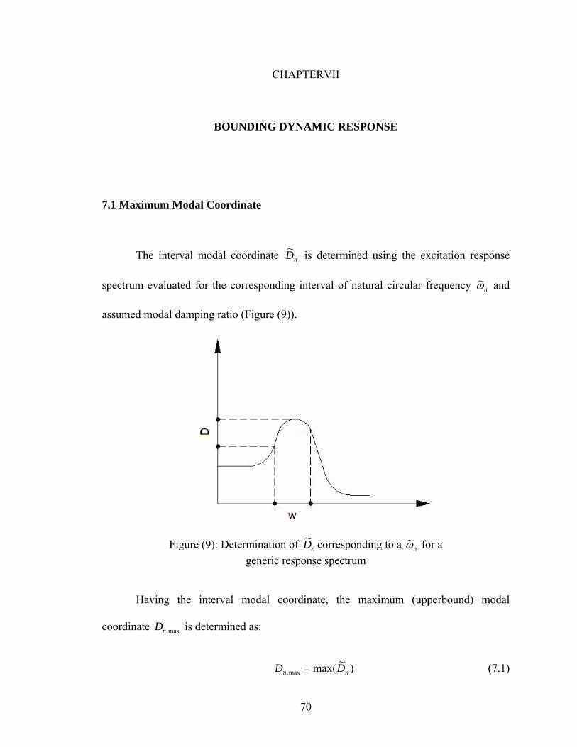
The interval modal coordinate nD~ is determined using the excitation response

spectrum evaluated for the corresponding interval of natural circular frequency nω~ and

assumed modal damping ratio (Figure (9)).

Figure (9): Determination of nD~ corresponding to a nω~ for a generic response spectrum

Having the interval modal coordinate, the maximum (upperbound) modal

coordinate max,nD is determined as:

)~max(max, nn DD = (7.1)

71

7.2 Interval Modal Participation Factor

If excitation is proportional, the interval modal participation factor is obtained as:

~][~

~~~n

Tn

Tn

n

Tn

n MP

MP

ϕϕϕϕ

==Γ (7.2)

7.3 Maximum Modal Response

The maximum modal response is determined as the maximum of the product of

the maximum modal coordinate, the interval modal participation factor and the interval

mode shape as:

( )~)~)((max max,max, nnnn DU ϕΓ= (7.3)

To achieve sharper results, functional dependency of intervals in the

multiplicative terms must be considered. Maximum modal response, Eq.(7.3), is

expanded using the definitions of the interval mode shapes and the interval modal

participation factor, Eqs.(6.21,7.2) as:

]])][][][][)[)(((])][][)[((

]][)[]][[)()(((])[]][[)(((

])][][)[((][

]][)[)(((][)max[(

1 1 1

1 1 1

1

1max,max,

n

n

N

i

N

i

N

jjninji

Tnnini

Tn

N

i

N

i

N

jinnin

Tjinin

Ti

n

N

iini

Tnn

Tn

N

iinn

Tin

T

nn

ECMECMEC

ECECPIECP

ECMM

ECPIPDU

ϕϕεεϕϕεϕ

ϕεεϕε

ϕεϕϕϕ

ϕεϕ

∑ ∑∑

∑ ∑∑

∑

∑

= = =

= = =

=

=

+

+

++

++= L

(7.4)

72

Thus, considering the dependency of the intervals of uncertainty for each element, )( iε ,

the sharper results for maximum modal response are obtained.

7.4 Maximum Total Responses

Finally, the contributions of all maximum modal responses are combined to

determine the maximum total response using SRSS or other combination methods.

∑=

=N

nnUU

1

2max,max (7.5)

7.5 Summary

The interval response spectrum analysis (IRSA) is summarized as following:

1. Define the uncertain physical or geometrical characteristics with closed intervals.

• Determine the interval stiffness matrix ]~[K and interval mass matrix ]~[M .

• Assume the modal damping ratio nζ .

2. Perform an interval eigenvalue problem between the interval stiffness and interval

mass matrices.

• Determine the bounds on natural circular frequencies nω~ (interval natural

frequencies).

• Determine the bounds on mode shapes ~ nϕ (interval mode shapes).

73

3. Compute the maximum modal response.

• Determine the interval modal coordinate nD~ and the maximum modal coordinate

max,nD using the excitation response spectrum for the bounds of corresponding

natural circular frequency and assumed modal damping ratio.

• Determine the interval modal participation factor nΓ~ .

• Compute the maximum modal response as the product of the maximum modal

coordinate, the interval modal participation factor and the interval mode shape.

4. Combine the contributions of all maximum modal responses to determine the

maximum total reponse using SRSS or other combination methods.

74

CHAPTER VIII

NUMERICAL EXAMPLES AND BEHAVIOR OF IRSA METHOD

In this section, the numerical behavior of the IRSA algorithm will be investigated.

The computational complexity associated with the behavior will be explored as well as

overestimation of interval bounds introduced by the algorithm.

The loss of sharpness as a function of initial interval width will be studied from

several example problems.

In addition, the effect of problem size on the interval estimation will be explored

and each step in the three step IRSA method (bounds on natural frequencies, mode

shapes and response) will be studied.

8.1 Examples for Bounds on Natural Frequencies

The first step in IRSA method is the construction of interval bounds on the natural

frequencies of a structure or a finite element mesh. The following problems obtains the

bounds on natural frequencies for different systems.

75

Problem 8.1.1

As the first problem, the bounds on the natural frequencies for a 2D three-element

truss with interval uncertainty present in the modulus of elasticity of each element are

determined (Figure (10)).

Figure (10): Equilateral truss with material uncertainty

Using the structural stiffness, the lumped mass matrices and the intervals of

material uncertainty as:

EEEE

EEEE

EEEE

UL

UL

UL

])2.1,8.0([],[~])3.1,7.0([],[~])1.1,9.0([],[~

333

222

111

==

==

==

the deterministic eigenvalue problems for maximum and minimum natural frequencies,

Eqs.(6.14) and (6.15), become:

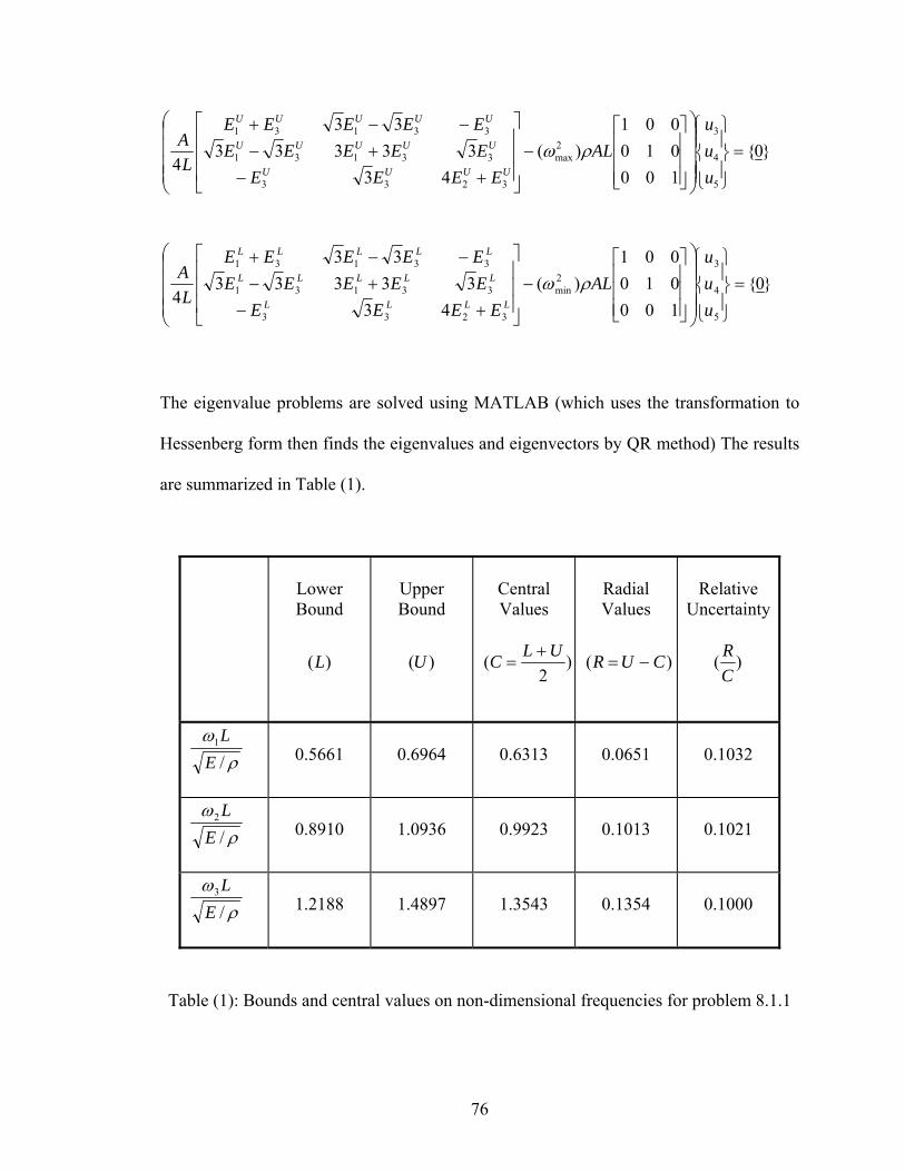
76

0100010001

)(43

3333333

45

4

32max

3233

33131

33131

=⎪⎭

⎪⎬

⎫

⎪⎩

⎪⎨

⎧

⎟⎟⎟⎟

⎠

⎞

⎜⎜⎜⎜

⎝

⎛

⎥⎥⎥

⎦

⎤

⎢⎢⎢

⎣

⎡−

⎥⎥⎥

⎦

⎤

⎢⎢⎢

⎣

⎡

+−+−

−−+

uuu

ALEEEE

EEEEEEEEEE

LA

UUUU

UUUUU

UUUUU

ρω

0100010001

)(43

3333333

45

4

32min

3233

33131

33131

=⎪⎭

⎪⎬

⎫

⎪⎩

⎪⎨

⎧

⎟⎟⎟⎟

⎠

⎞

⎜⎜⎜⎜

⎝

⎛

⎥⎥⎥

⎦

⎤

⎢⎢⎢

⎣

⎡−

⎥⎥⎥

⎦

⎤

⎢⎢⎢

⎣

⎡

+−+−

−−+

uuu

ALEEEE

EEEEEEEEEE

LA

LLLL

LLLLL

LLLLL

ρω

The eigenvalue problems are solved using MATLAB (which uses the transformation to

Hessenberg form then finds the eigenvalues and eigenvectors by QR method) The results

are summarized in Table (1).

Table (1): Bounds and central values on non-dimensional frequencies for problem 8.1.1

Lower Bound

)(L

Upper Bound

)(U

Central Values

)2

( ULC +=

Radial Values

)( CUR −=

Relative

Uncertainty

)(CR

ρω

/1

EL

0.5661

0.6964

0.6313

0.0651

0.1032

ρω

/2

EL

0.8910

1.0936

0.9923

0.1013

0.1021

ρω

/3

EL

1.2188

1.4897

1.3543

0.1354

0.1000

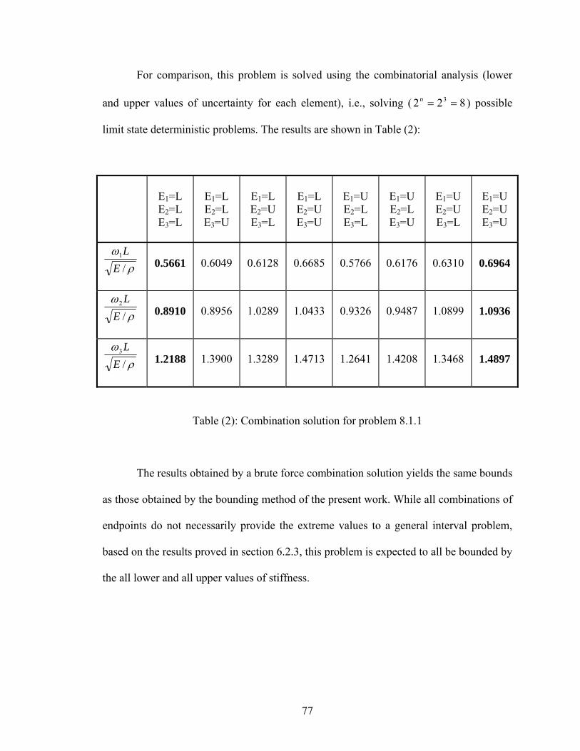
77

For comparison, this problem is solved using the combinatorial analysis (lower

and upper values of uncertainty for each element), i.e., solving ( 822 3 ==n ) possible

limit state deterministic problems. The results are shown in Table (2):

E1=L E2=L E3=L

E1=L E2=L E3=U

E1=L E2=U E3=L

E1=L E2=U E3=U

E1=U E2=L E3=L

E1=U E2=L E3=U

E1=U E2=U E3=L

E1=U E2=U E3=U

ρω

/1

EL

0.5661

0.6049

0.6128

0.6685

0.5766

0.6176

0.6310

0.6964

ρω

/2

EL

0.8910

0.8956

1.0289

1.0433

0.9326

0.9487

1.0899

1.0936

ρω

/3

EL

1.2188

1.3900

1.3289

1.4713

1.2641

1.4208

1.3468

1.4897

Table (2): Combination solution for problem 8.1.1

The results obtained by a brute force combination solution yields the same bounds

as those obtained by the bounding method of the present work. While all combinations of

endpoints do not necessarily provide the extreme values to a general interval problem,

based on the results proved in section 6.2.3, this problem is expected to all be bounded by

the all lower and all upper values of stiffness.

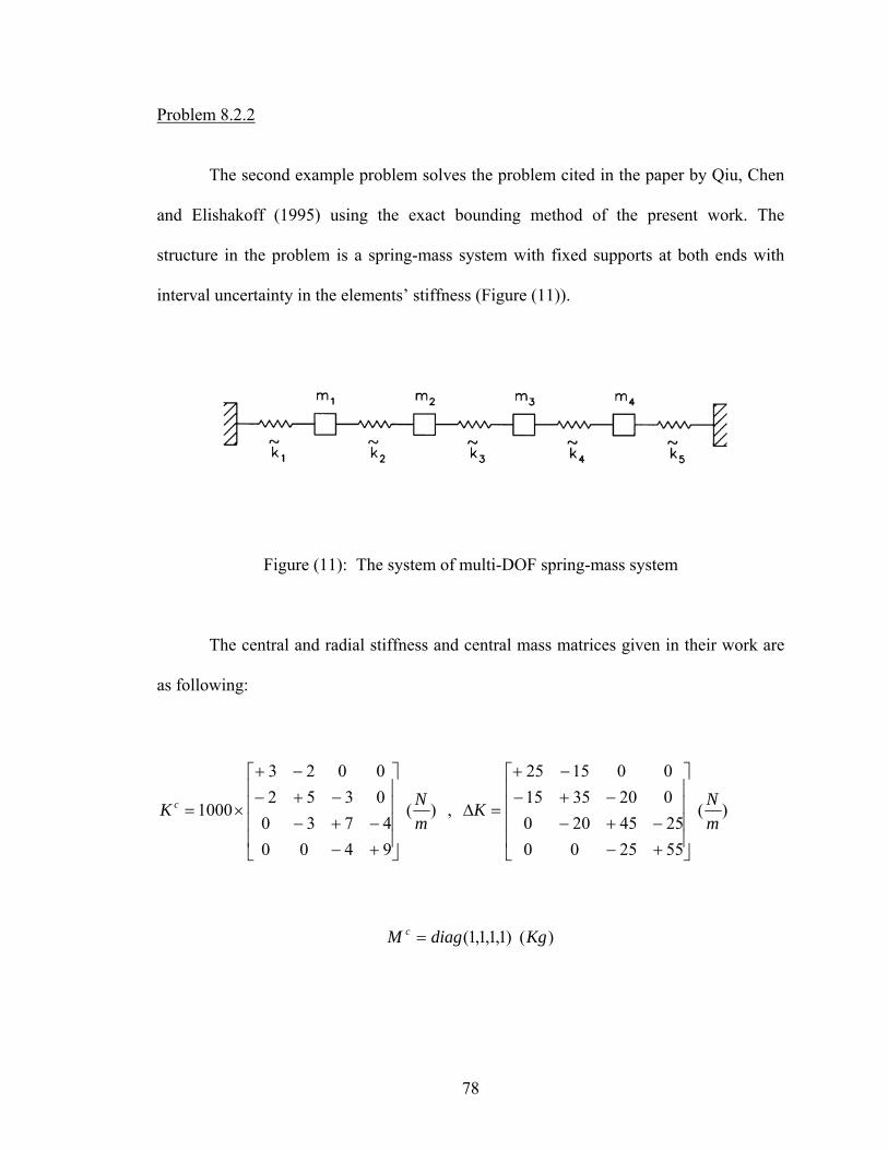
78

Problem 8.2.2

The second example problem solves the problem cited in the paper by Qiu, Chen

and Elishakoff (1995) using the exact bounding method of the present work. The

structure in the problem is a spring-mass system with fixed supports at both ends with

interval uncertainty in the elements’ stiffness (Figure (11)).

Figure (11): The system of multi-DOF spring-mass system

The central and radial stiffness and central mass matrices given in their work are

as following:

)(

94004730

03520023

1000mNK c

⎥⎥⎥⎥

⎦

⎤

⎢⎢⎢⎢

⎣

⎡

+−−+−

−+−−+

×= , )(

55250025452000203515001525

mNK

⎥⎥⎥⎥

⎦

⎤

⎢⎢⎢⎢

⎣

⎡

+−−+−

−+−−+

=∆

)()1,1,1,1( KgdiagM c =

79

Having the problem input information, the individual element interval stiffness

matrices )/( mN are back-calculated as:

The eigenvalue problem is solved using the method presented in this work and the results

for eigevalues )sec/1( 2 are summarized in Table (3).

Table (3): Solution of the example problem 8.1.2 using the present method

Lower Bound

Upper Bound

Central Values

Radial Values

Relative

Uncertainty

1~λ

898.20

912.12

905.16

6.96

0.00769

2~λ

3364.86

3414.84

3389.85

24.99

0.00737

3~λ

7016.10

7112.82

7064.46

48.36

0.00684

4~λ

12560.84

12720.23

12640.53

79.69

0.00630

⎥⎦

⎤⎢⎣

⎡+−−+

=

⎥⎦

⎤⎢⎣

⎡+−−+

=⎥⎦

⎤⎢⎣

⎡+−−+

=

⎥⎦

⎤⎢⎣

⎡+−−+

=⎥⎦

⎤⎢⎣

⎡+−−+

=

1111

])5030,4970([~

1111

])4025,3975([~1111

])3020,2980([~

1111

])2015,1985([~1111

])1010,990([~

5

43

21

K

KK

KK

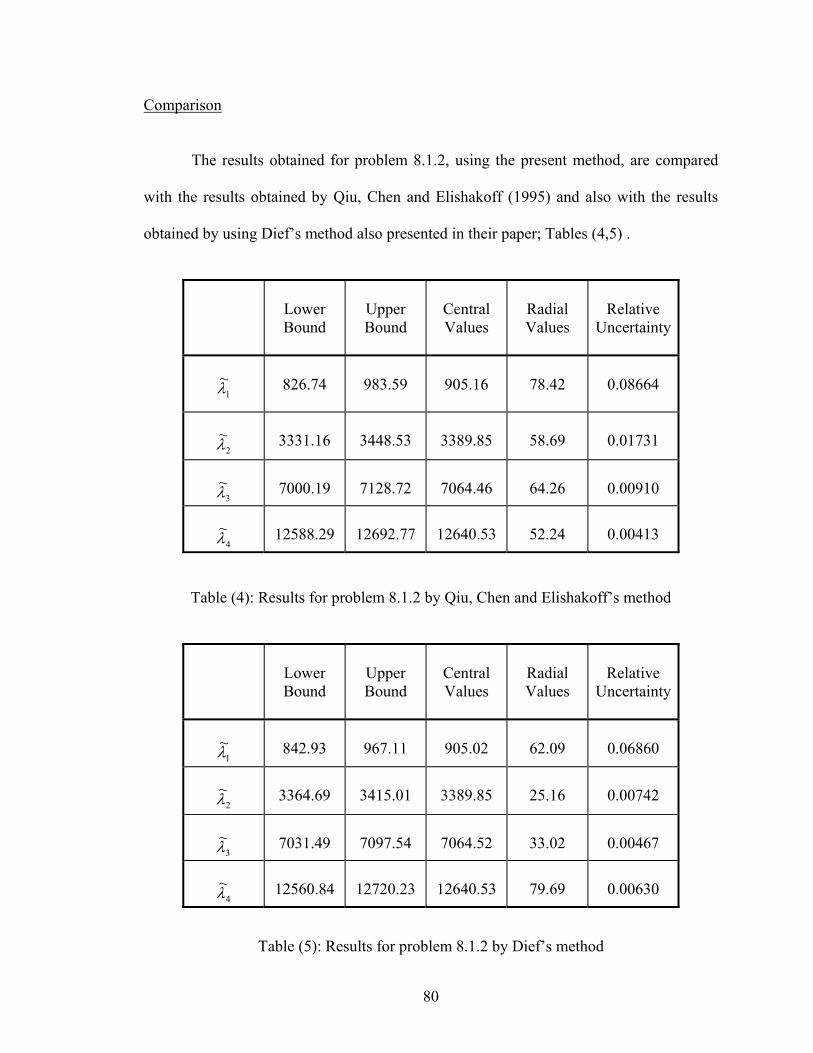
80

Comparison

The results obtained for problem 8.1.2, using the present method, are compared

with the results obtained by Qiu, Chen and Elishakoff (1995) and also with the results

obtained by using Dief’s method also presented in their paper; Tables (4,5) .

Table (4): Results for problem 8.1.2 by Qiu, Chen and Elishakoff’s method

Table (5): Results for problem 8.1.2 by Dief’s method

Lower Bound

Upper Bound

Central Values

Radial Values

Relative

Uncertainty

1~λ

826.74

983.59

905.16

78.42

0.08664

2~λ

3331.16

3448.53

3389.85

58.69

0.01731

3~λ

7000.19

7128.72

7064.46

64.26

0.00910

4~λ

12588.29

12692.77

12640.53

52.24

0.00413

Lower Bound

Upper Bound

Central Values

Radial Values

Relative

Uncertainty

1~λ

842.93

967.11

905.02

62.09

0.06860

2~λ

3364.69

3415.01

3389.85

25.16

0.00742

3

~λ

7031.49

7097.54

7064.52

33.02

0.00467

4~λ

12560.84

12720.23

12640.53

79.69

0.00630

81

Discussion

The results by Qiu, Chen and Elishakoff (1995) are wider than the present results

for lower eigenvalues, however, for higher eigenvalues, their method does not include the

whole range of uncertainty. This underestimation is perhaps due to the usage the non-

perturbed eigenvectors to obtain the bounds on eigenvalues.

Using Dief’s method, the lower eigenvalues have a wider range of uncertainty

than the present exact results. At high frequencies, Dief’s method provides better bounds.

However, all of the bounds provided by Dief’s method contain the correct values.

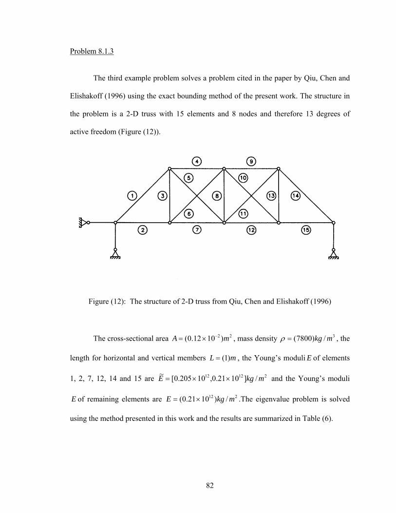
82

Problem 8.1.3

The third example problem solves a problem cited in the paper by Qiu, Chen and

Elishakoff (1996) using the exact bounding method of the present work. The structure in

the problem is a 2-D truss with 15 elements and 8 nodes and therefore 13 degrees of

active freedom (Figure (12)).

Figure (12): The structure of 2-D truss from Qiu, Chen and Elishakoff (1996)

The cross-sectional area 22 )1012.0( mA −×= , mass density 3/)7800( mkg=ρ , the

length for horizontal and vertical members mL )1(= , the Young’s moduli E of elements

1, 2, 7, 12, 14 and 15 are 21212 /]1021.0,10205.0[~ mkgE ××= and the Young’s moduli

E of remaining elements are 212 /)1021.0( mkgE ×= .The eigenvalue problem is solved

using the method presented in this work and the results are summarized in Table (6).

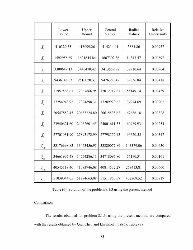
83

Table (6): Solution of the problem 8.1.3 using the present method

Comparison

The results obtained for problem 8.1.3, using the present method, are compared

with the results obtained by Qiu, Chen and Elishakoff (1996); Table (7).

Lower Bound

Upper Bound

Central Values

Radial Values

Relative

Uncertainty

1~λ

410329.55

418099.26

414214.41

3884.86

0.00937

2~λ

1592958.89

1621645.84

1607302.36

14343.47

0.00892

3~λ

3380649.13

3446470.42

3413559.78

32910.64

0.00964

4~λ

9436746.63

9516020.31

9476383.47

39636.84

0.00418

5~λ

11957568.67

12067866.95

12012717.81

55149.14

0.00459

6

~λ

17254948.92

17324898.31

17289923.62

34974.69

0.00202

7~λ

20547852.45

20683224.80

20615538.62

67686.18

0.00328

8

~λ

23940621.60

24062601.45

24001611.53

60989.93

0.00254

9~λ

27701931.90

27895172.99

27798552.45

96620.55

0.00347

10~λ

33176698.83

33463456.95

33320077.89

143379.06

0.00430

11~λ

34661905.48

34774286.11

34718095.80

56190.31

0.00161

12~λ

40545118.46

41083946.08

40814532.27

269413.81

0.00660

13~λ

51039044.05

51984663.08

51511853.57

472809.52

0.00917

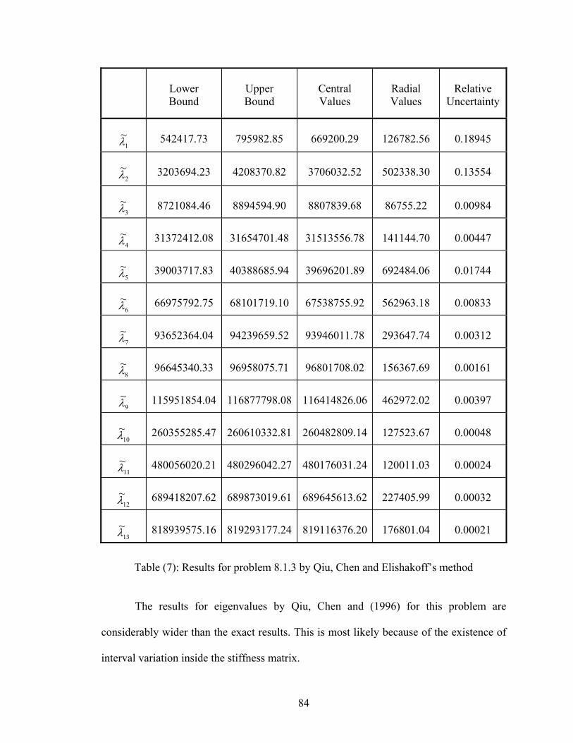
84

Table (7): Results for problem 8.1.3 by Qiu, Chen and Elishakoff’s method

The results for eigenvalues by Qiu, Chen and (1996) for this problem are

considerably wider than the exact results. This is most likely because of the existence of

interval variation inside the stiffness matrix.

Lower Bound

Upper Bound

Central Values

Radial Values

Relative

Uncertainty

1~λ

542417.73

795982.85

669200.29

126782.56

0.18945

2~λ

3203694.23

4208370.82

3706032.52

502338.30

0.13554

3~λ

8721084.46

8894594.90

8807839.68

86755.22

0.00984

4~λ

31372412.08

31654701.48

31513556.78

141144.70

0.00447

5~λ

39003717.83

40388685.94

39696201.89

692484.06

0.01744

6

~λ

66975792.75

68101719.10

67538755.92

562963.18

0.00833

7~λ

93652364.04

94239659.52

93946011.78

293647.74

0.00312

8

~λ

96645340.33

96958075.71

96801708.02

156367.69

0.00161

9~λ

115951854.04

116877798.08

116414826.06

462972.02

0.00397

10~λ

260355285.47

260610332.81

260482809.14

127523.67

0.00048

11~λ

480056020.21

480296042.27

480176031.24

120011.03

0.00024

12~λ

689418207.62

689873019.61

689645613.62

227405.99

0.00032

13~λ

818939575.16

819293177.24

819116376.20

176801.04

0.00021

85

In the eigenvalue step in the IRSA, the computational effort is twice than that

required for deterministic analysis. Directional rounding could be used to provide bounds

that include the impact of truncation errors.

The additional cost of a true “all interval” method would depend on the computer

hardware and the specific method to calculate eigenvalues. In the first step of the IRSA

method, only the effects of problem size and initial interval widths determine the

behavior of the underlying eigenvalue method. Any interval overestimation will be

caused by other steps in the algorithm.

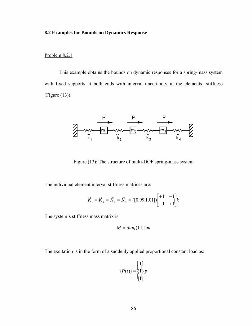
86

8.2 Examples for Bounds on Dynamics Response

Problem 8.2.1

This example obtains the bounds on dynamic responses for a spring-mass system

with fixed supports at both ends with interval uncertainty in the elements’ stiffness

(Figure (13)).

Figure (13): The structure of multi-DOF spring-mass system

The individual element interval stiffness matrices are:

kKKKK ⎥⎦

⎤⎢⎣

⎡+−−+

====1111

])01.1,99.0([~~~~4321

The system’s stiffness mass matrix is:

mdiagM )1,1,1(=

The excitation is in the form of a suddenly applied proportional constant load as:

ptP⎪⎭

⎪⎬

⎫

⎪⎩

⎪⎨

⎧=

111

)(

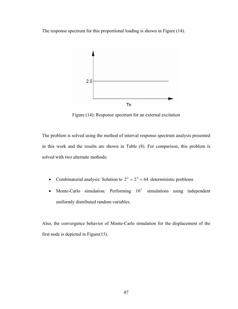
87

The response spectrum for this proportional loading is shown in Figure (14).

Figure (14): Response spectrum for an external excitation

The problem is solved using the method of interval response spectrum analysis presented

in this work and the results are shown in Table (8). For comparison, this problem is

solved with two alternate methods:

• Combinatorial analysis: Solution to 6422 4 ==n deterministic problems

• Monte-Carlo simulation: Performing 710 simulations using independent

uniformly distributed random variables.

Also, the convergence behavior of Monte-Carlo simulation for the displacement of the

first node is depicted in Figure(15).

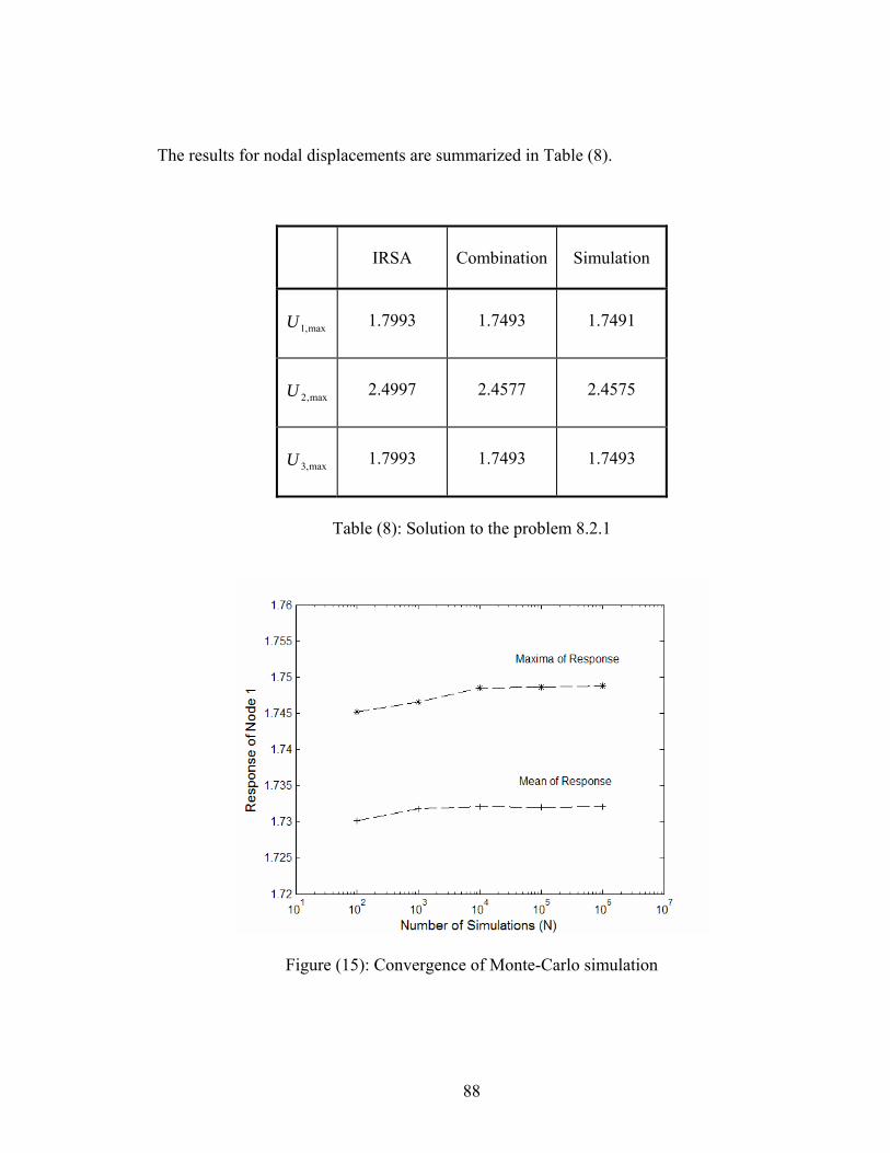
88

The results for nodal displacements are summarized in Table (8).

IRSA

Combination

Simulation

max,1U

1.7993

1.7493

1.7491

max,2U

2.4997

2.4577

2.4575

max,3U

1.7993

1.7493

1.7493

Table (8): Solution to the problem 8.2.1

Figure (15): Convergence of Monte-Carlo simulation

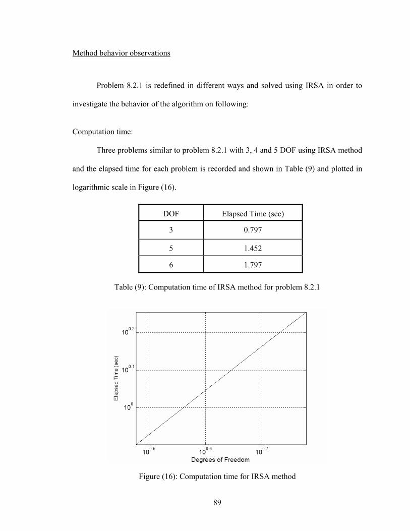
89

Method behavior observations

Problem 8.2.1 is redefined in different ways and solved using IRSA in order to

investigate the behavior of the algorithm on following:

Computation time:

Three problems similar to problem 8.2.1 with 3, 4 and 5 DOF using IRSA method

and the elapsed time for each problem is recorded and shown in Table (9) and plotted in

logarithmic scale in Figure (16).

DOF Elapsed Time (sec)

3 0.797

5 1.452

6 1.797

Table (9): Computation time of IRSA method for problem 8.2.1

Figure (16): Computation time for IRSA method

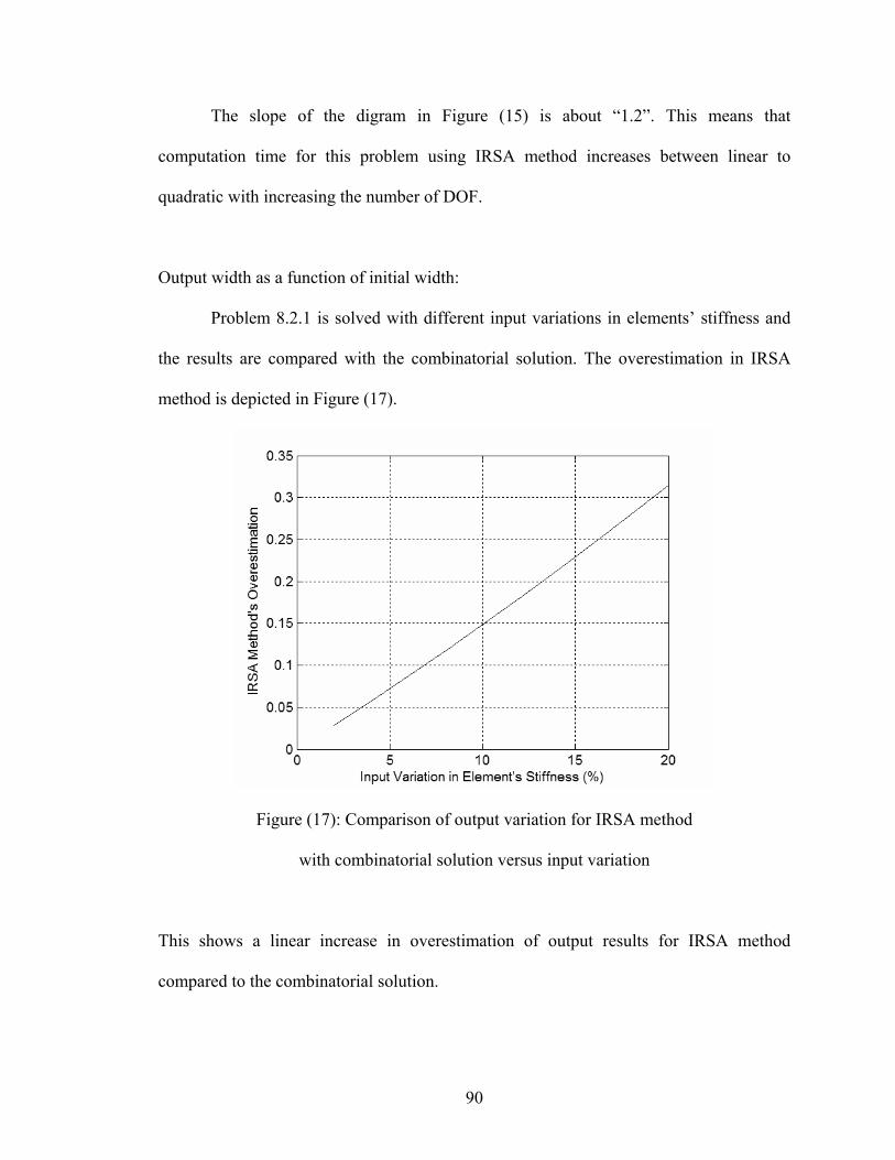
90

The slope of the digram in Figure (15) is about “1.2”. This means that

computation time for this problem using IRSA method increases between linear to

quadratic with increasing the number of DOF.

Output width as a function of initial width:

Problem 8.2.1 is solved with different input variations in elements’ stiffness and

the results are compared with the combinatorial solution. The overestimation in IRSA

method is depicted in Figure (17).

Figure (17): Comparison of output variation for IRSA method

with combinatorial solution versus input variation

This shows a linear increase in overestimation of output results for IRSA method

compared to the combinatorial solution.

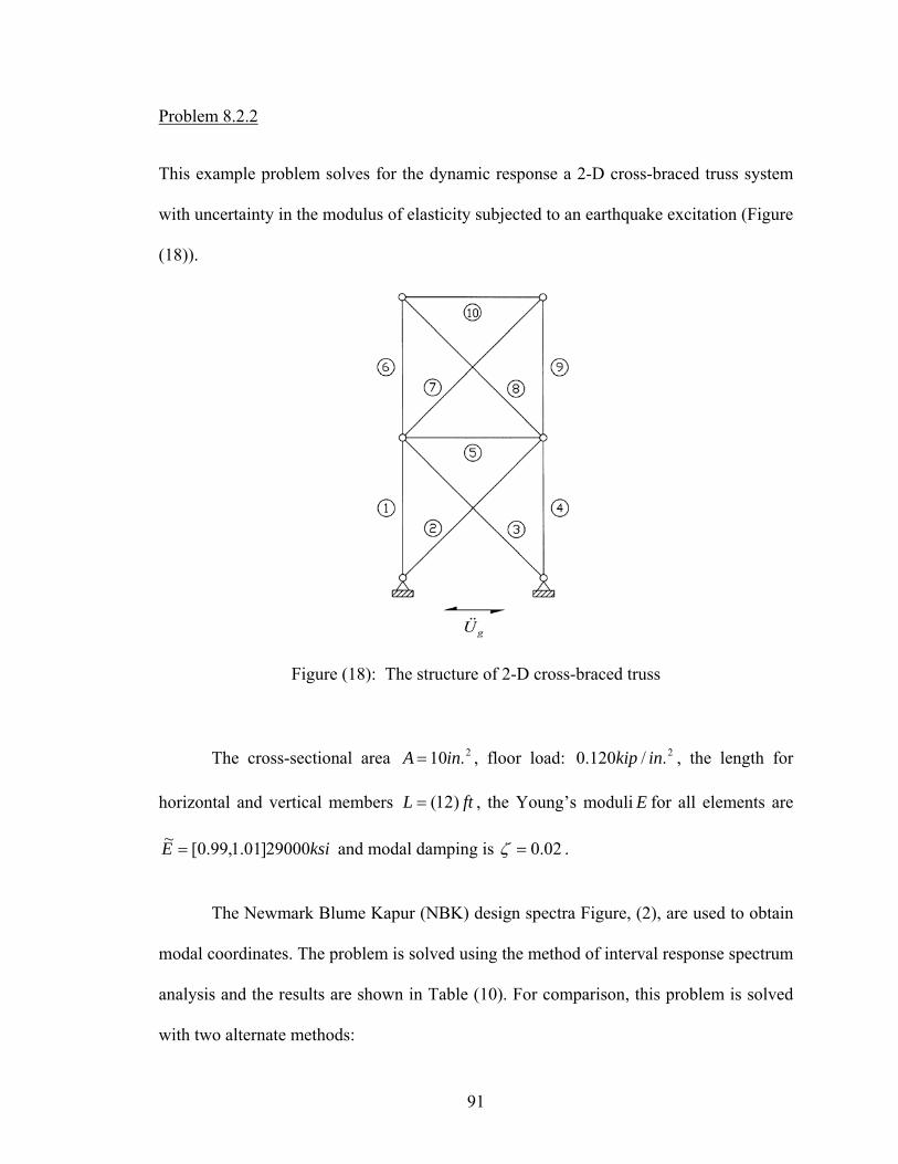
91

Problem 8.2.2

This example problem solves for the dynamic response a 2-D cross-braced truss system

with uncertainty in the modulus of elasticity subjected to an earthquake excitation (Figure

(18)).

Figure (18): The structure of 2-D cross-braced truss

The cross-sectional area 2.10inA = , floor load: 2./120.0 inkip , the length for

horizontal and vertical members ftL )12(= , the Young’s moduli E for all elements are

ksiE 29000]01.1,99.0[~ = and modal damping is 02.0=ζ .

The Newmark Blume Kapur (NBK) design spectra Figure, (2), are used to obtain

modal coordinates. The problem is solved using the method of interval response spectrum

analysis and the results are shown in Table (10). For comparison, this problem is solved

with two alternate methods:

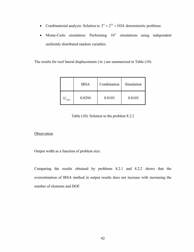
92

• Combinatorial analysis: Solution to 102422 10 ==n deterministic problems

• Monte-Carlo simulation: Performing 410 simulations using independent

uniformly distributed random variables.

The results for roof lateral displacements ( .in ) are summarized in Table (10).

IRSA

Combination

Simulation

maxU

0.8294

0.8103

0.8103

Table (10): Solution to the problem 8.2.2

Observation

Output width as a function of problem size:

Comparing the results obtained by problems 8.2.1 and 8.2.2 shows that the

overestimation of IRSA method in output results does not increase with increasing the

number of elements and DOF.

93

CHAPTER IX

CONCLUSIONS

• A finite-element based method for dynamic analysis of structures with interval

uncertainty in structure’s stiffness or mass properties is presented.

• In the presence of any interval uncertainty in the characteristics of structural

elements, the proposed method of interval response spectrum analysis (IRSA) is

capable to obtain the nearly sharp bounds on the structure’s dynamic response.

• IRSA is computationally feasible and it shows that the bounds on the dynamic

response can be obtained without combinatorial or Monte-Carlo simulation

procedures.

• The solutions to only two non-interval eigenvalue problems are sufficient to bound

the natural frequencies of the structure. Based on the given mathematical proof, the

obtained bounds on natural frequencies are exact and sharp.

• Computation time for the algorithm increases between linear to quadratic with

increasing the number of degrees of freedom.

• Some conservative overestimation in dynamic response occurs because of

linearization in formation of bounds of mode shapes and also, the dependency of

intervals in the dynamic response formulation. These are the expected cause of loss of

sharpness in the interval results.

94

• The overestimation of output results for IRSA method linearly increases with

increasing the number of degrees of freedom in comparison with the combinatorial

solution.

• The solution of the solved problems for dynamic response indicates that the output

overestimation does not increase as the problem size increases.

• The computational efficiency of the proposed method makes IRSA an attractive

method to introduce uncertainty into dynamic analysis.

95

REFERENCE Alefeld, G. & Herzberger, J., 1983 “Introduction to Linear Computation ” , NewYork: Academic Press. Anderson, A.W., et al 1952 “Lateral Forces on Earthquake and Wind”, Trans. ASCE, Vol. 117, p. 716. Archimedes (287-212 B.C.); by Heath, T.L., 1897 “The Works of Archimedes”, Cambridge, Cambridge University Press. Bellman, Richard, 1960 “Introduction to Matrix Analysis ” , McGrawHill, New York. Biggs, J. M.,1964 “Introduction to Structural Dynamics” McGraw-Hill, Inc. Biot, M. A., 1932 “Vibrations of Buildings during Earthquake”, Chapter II in Ph.D. Thesis No. 259 entitled “Transient Oscillations in Elastic System”, Aeronautics Department, Calif. Inst. of Tech., Pasadena, California, U.S.A. Clough, R.W., & Penzien, J. 1993 “Dynamics of Structures”, McGraw-Hill, New York. Dennis Jr. , D.E. Jr. & Schnabel, R.B. 1983 “Numerical Methods for Unconstrained Optimization and Nonlinear Equations” Prentice-Hall, Englewood Cliffs. Dief, A., 1991 “Advanced Matrix theory for Scientists and Engineers”,pp.262-281. Abacus Press (1991) Dwyer, P. S., 1951 “Linear Computations ” , New York: John Wiley. Housner, G. W., 1959 “Behavior of Structures During Earthquake” Proc. ASCE Vol. 85, No. EM 4 p. 109. Hudson, D. E., 1956 “Response Spectrum Techniques in Engineering Seismology” Proc. World Conf. on Earthquake Eng. Earthquake Engineering Research Institute, Berkeley, California. Gasparini, Dario A., 2003, Class-notes for ECIV-424 “Structural Dynamics”. Department of Civil Engineering, Case Western Reserve University, Cleveland, Ohio. Qiu, Z. P., Chen, S. H., and Elishakoff, I. 1995, “Natural frequencies of structures with uncertain but non-random parameters”, J. Optimization Theor. Appl. 86, 669-683 (1995).

96

Qiu, Z. P., Chen, S. H., and Elishakoff, I. 1996, “Non-probabilistic Eigenvalue Problem for Structures with Uncertain Parameters via Interval Analysis”,Chaos, soliton and fractals,7, 303-308 (1996). Moore, Ramon E., 1966 “Interval Analysis”, Prentice Hall, Englewood, NJ. Newmark, N. M., 1962 “A Method of Computation for Structural Dynamics”, Trans. ASCE, Vol. 127, pt. 1, pp. 1406-1435. Muhanna, Rafi L. & Mullen, Robert L., 2001. “Uncertainty in Mechanics Problems-Interval-Based Approach”. Journal of Engineering Mechanics June-2001, pp.557-566. Muhanna, R. L. and Mullen, R. L., “Formulation of Fuzzy Finite Element Methods for Mechanics Problems”, Computer-Aided Civil and Infrastructure Engineering, 14, pp. 107-117, 1999. Mullen, Robert L., 2003, Class-notes for ECIV-420 “Finite Element Analysis I”. Department of Civil Engineering, Case Western Reserve University, Cleveland, Ohio. Newmark, N. M., Blume, J. A. and Kapur, K. K. 1973 “Seismic Design Spectra for Nuclear Power Plants”. J. Power Division, Proc ASCE, Vol. 99, No. P02, 287-303. Neumaier, Arnold, 1990 “Interval Methods for Systems of Equations”, Cambridge University Press, Cambridge. Looney, C. T. G., 1954 “Behavior of Structures Subjected to a Forced Vibration”, Proc. ASCE, Vol. 80, Separate No. 451. Rosenblueth, E. & Bustamente, J. I., 1962 “Distribution of Structural Response to Earthquakes”, Proc. ASCE, Vol. 88, No. EM 3 p. 75. Sunaga, T., 1958 “Theory of an Interval Algebra and its Application to Numerical Analysis” RAAG Memoirs II 2, 547-565. Tokyo, Japan. Stewart, G.W. & Sun, Ji-Guang, 1990 “Matrix perturbation theory” Academic Press, Boston, MA. Strang, Gilbert, 1976 “Linear Algebra and its Applications”, Massachusetts Institute of Technology. Trefethen, L. N. & Bau III, D., 1997 “Numerical Linear Algebra”, SIAM. Veletsos, A. S. & Newmark, N. M., 1957 “Natural Frequencies of Continuous Flexural Members”, Trans. ASCE, Vol. 122, p. 249. Young, R. C., 1931 “The Algebra of Many-Valued Quantities” Mathematics Annalen 104, 260-290.