Medical Engineering and Physics 47 (2017) 2–12

Contents lists available at ScienceDirect

Medical Engineering and Physics

journal homepage: www.elsevier.com/locate/medengphy

Finite element analysis of TAVI: Impact of native aortic root

computational modeling strategies on simulation outcomes

Alice Finotello

a , Simone Morganti b , ∗, Ferdinando Auricchio c

a Department of Experimental Medicine, University of Genova, Largo R. Benzi, 10, 16132 Genova, Italy b Department of Electrical, Computer, and Biomedical Engineering, University of Pavia, Via Ferrata 5, 27100 Pavia, Italy c Department of Civil Engineering and Architecture, University of Pavia, Via Ferrata 3, 27100 Pavia, Italy

a r t i c l e i n f o

Article history:

Received 16 February 2017

Revised 21 June 2017

Accepted 25 June 2017

Keywords:

Transcatheter aortic valve implantation

Patient-specific modeling

Finite element analysis

a b s t r a c t

In the last few years, several studies, each with different aim and modeling detail, have been proposed

to investigate transcatheter aortic valve implantation (TAVI) with finite elements. The present work fo-

cuses on the patient-specific finite element modeling of the aortic valve complex. In particular, we aim

at investigating how different modeling strategies in terms of material models/properties and discretiza-

tion procedures can impact analysis results. Four different choices both for the mesh size (from 20 k

elements to 200 k elements) and for the material model (from rigid to hyperelastic anisotropic) are con-

sidered. Different approaches for modeling calcifications are also taken into account. Post-operative CT

data of the real implant are used as reference solution with the aim of outlining a trade-off between

computational model complexity and reliability of the results.

© 2017 IPEM. Published by Elsevier Ltd. All rights reserved.

p

d

i

t

t

s

l

p

a

s

p

p

t

s

s

h

p

f

1. Introduction

Aortic Stenosis (AS) is the most common form of valvular heart

disease in developed countries, occurring in 3% of people older

than 65 [1] . It is a degenerative disease of the aortic valve, com-

promising its function of regulating blood flow from the left ven-

tricle to the aorta, with significant consequences on morbidity and

mortality of patients, thus representing a current relevant clinical

problem.

In the last decade, transcatheter aortic valve implantation (TAVI)

has become the established treatment option for patients at high

surgical risk, representing nearly the 30% of procedures for elderly

patients with severe AS, not suitable candidates for conventional

open heart surgery [2] . It is estimated that, since the first-in-man

TAVI in 2002, more than 100.000 patients worldwide benefited

from this revolutionary procedure [3] . However, despite the clinical

success, there are still some complications associated with TAVI;

the most relevant being post-operative paravalvular leakage, but

also aortic root rupture, prosthesis migration, left bundle branch

impairment may occur [4] , which are contraindications typically

related to the mutual interaction between the device and the aor-

tic root wall.

∗ Corresponding author.

E-mail address: simone.morganti@unipv.it (S. Morganti).

t

e

s

r

a

a

http://dx.doi.org/10.1016/j.medengphy.2017.06.045

1350-4533/© 2017 IPEM. Published by Elsevier Ltd. All rights reserved.

For clinicians, such complications are difficult to predict due to

atient variability, especially in terms of aortic root geometry and

istribution and dimension of calcific plaques. For this reason, clin-

cal operators look with enormous interest at tools potentially able

o allow the surgeon to select the optimal valve for a specific pa-

ient, i.e., tools able to give predictive evaluation of the prosthe-

is post-operative performance (principally intended as degree of

eaflet coaptation and entity of possible paravalvular leakage). Such

rocedure outcomes depend on the choice of the device, on the

dopted implantation strategy, and, of course, on the pre-operative

pecific native valve configuration [5] .

In this context of personalized medicine, patient-specific com-

utational simulations, based on pre-operative images, represent a

owerful tool capable to obtain such predictive information about

he behavior of the device, both during delivery and after expan-

ion. A detailed review about the state of the art of patient-specific

imulations of TAVI is available in Vy et al. [6] .

Since the first finite element study of TAVI [7] , several authors

ave proposed different modeling strategies of the percutaneous

rocedure either to investigate the hemodynamic environment be-

ore and after TAVI [8] , or to explore the feasibility of TAVI in pa-

ient specific morphologies [9] . Computer-based simulations can be

mployed also to reconstruct the loading forces induced by the

tent on the aortic valvular complex [10] , as well as to evaluate the

adial force produced by the self-expandable or balloon expand-

ble devices [11] . The prediction of the outcomes of percutaneous

ortic valve implantation through numerical simulations has been

A. Finotello et al. / Medical Engineering and Physics 47 (2017) 2–12 3

e

b

C

(

o

t

G

t

c

e

c

i

3

p

F

i

f

r

e

s

b

i

f

m

o

t

d

r

e

a

a

t

t

a

c

b

r

s

p

c

2

o

f

s

c

c

c

c

b

o

t

t

n

2

t

Table 1

List of parameters used to reproduce the Nitinol behavior taken from Au-

ricchio et al. [23] .

Nitinol material parameters

Austenite Young’s modulus 51,700 MPa

Austenite Poisson’s Ratio 0.3

Martensite Young’s modulus 47,800 M Pa

Martensite Poisson’s Ratio 0.3

Transformation strain 0.063

Loading 6.527

Loading start of transformation stress 600 M Pa

Loading end of transformation stress 670 MPa

Temperature 37 o C

Unloading 6.527

Unloading start of transformation stress 288 MPa

Unloading end of transformation stress 254 MPa

Start of transformation stress (loading in compression) 900 MPa

Volumetric transformation strain 0.063

2

f

T

W

(

r

e

o

s

e

i

a

t

e

p

T

s

t

a

c

t

o

e

m

m

t

s

t

2

t

t

0

c

s

(

s

l

i

6

a

o

T

e

t

xtensively proposed for the two most common devices: the

alloon-expandable Edwards Sapien (Edwards Lifesciences, Irvine,

A, USA) [12–15] and the self expandable Medtronic Corevalve

Medtronic, Minneapolis, MN, USA) [16–19] . However, for this class

f very complex analyses, validation still represents a crucial issue.

Only very recently, few papers dealing with the validation of

he TAVI finite element simulation framework have been published.

rbic et al. [17] proposed for the first time an automatic procedure

o reconstruct patient-specific parametrical aortic valve models and

ompared the simulation results with postoperative images. How-

ver, very simplified aortic root and prosthetic device models were

onsidered. Schultz et al. [20] proposed a validation study (includ-

ng both Corevalve and Sapien implantation procedures) based on

9 patients; however, their work represents mainly a medical pa-

er and details about the adopted simulation strategy are missing.

inally, Bosmans et al. [16] conducted an interesting study compar-

ng finite element results and postoperative data, considering dif-

erent aortic wall thickness values and different (simplified) mate-

ial models.

When performing this kind of analyses, in fact, many param-

ters remain uncertain, including, for example, the real patient-

pecific mechanical properties of the aortic tissue which can only

e assumed on a statistical basis [21] without specific histological

nformation (usually not available for patients undergoing TAVI). In

act, while some analysis ingredients (like prosthesis geometry and

aterial properties) are well known in advance, others are not pre-

peratively available and may have significant impact on simula-

ion outcomes. Several studies, for example, agree that the use of

ifferent aortic root material models can deeply affect simulation

esults [6,18] .

Hence, the aim of the present work is to investigate how differ-

nt possible modeling strategies of the aortic valve complex may

ffect the finite element results and what is the balance between

cceptable accuracy for clinical purposes and reasonable computa-

ional efforts, again for clinical application. In particular, assuming

hat the device geometry and the material properties are known

nd that the morphology of the native valve can be reliably re-

onstructed from computed tomography (CT) images, the main ar-

itrary modeling choices are represented by the aortic valve and

oot material models and properties as well as by its discretization

trategy, focus of the present paper. Simulation results are com-

ared with a “exact solution” extracted from post-operative medi-

al images.

. Materials and Methods

An overview of the framework to evaluate TAVI post-procedural

utcomes is given in Fig. 1 .

A “high-fidelity” model of the prosthetic device is constructed

rom microCT images. Angio-CT scan data are used for patient-

pecific reconstruction of the aortic valve complex including calcifi-

ations, and intraoperative angiographic measurements are used to

orrectly replicate with finite elements the real implantation pro-

edure. These (green dots in Fig. 1 ) are assumed as reliable data in-

luded in the developed simulation framework. The impact of ar-

itrary modeling choices of the aortic district (red dots in Fig. 1 )

n simulation outcomes is investigated through a comparison be-

ween the obtained results and post-operative data.

In the following sections, we provide detailed descriptions of

he developed simulation framework, with particular focus on the

ative valve possible modeling choices.

.1. Prosthetic model

The prosthetic device chosen by the medical equipe for implan-

ation in the investigated clinical case is a Medtronic Corevalve size

9. The geometrical model of the Corevalve prosthesis is created

rom high-resolution micro-CT images of the real device sample.

he reconstructed STL file is imported in Rhinoceros 5.0 (McNell,

A, USA) where the CAD model of one elementary unit is built

see Fig. 2 a).

Matlab software (Mathworks Inc, Natick, MA, USA) is used to

eplicate in polar series the elementary unit in order to obtain the

ntire description of the device ( Fig. 2 b). Then, a structured mesh

f first-order hexahedral solid elements with a reduced integration

cheme is defined for the device model. In particular, C3D8R el-

ments in the Abaqus library (Simulia, Dassault Systèmes, Prov-

dence, RI, USA) were used. Approximately 80,0 0 0 elements are

dopted to discretize the entire structure using three elements in

he radial direction to prevent locking issues [22] . Material prop-

rties of the Nitinol alloy are considered according to the model

roposed by Auricchio et al. [23] . Material parameters are listed in

able 1 ; the density is set to 6.5 e −9 T mm

−3 . In this study, the tran-

catheter valve leaflets are not included since they do not affect

he mechanical behavior of the stent and its interaction with the

ortic root wall. A cylindrical surface, in the following labeled as

atheter , is built and used in the numerical analysis to reproduce

he crimping technique. The catheter is defined through a surface

btained by sweeping a cylindrical section having a radius length

qual to 22 mm and meshed using 11,040 quadrilateral surface ele-

ent with reduced integration (SFM3D4R). It is modeled as a rigid

aterial with a density equal to 6.7e −9 T mm

−3 . A frictionless con-

act is defined between the outer Corevalve surface and the inner

urface of the catheter, while a self-contact formulation is used for

he stent.

.2. Native aortic root model

Cardio-synchronized CT images of a 76 year-old male pa-

ient acquired at IRCCS Policlinico San Donato (Italy) in the dias-

olic phase with a Siemens MedCom Volume CT (pixel spacing:

.621/0.621; slice thickness: 1 mm) are used as starting point to

reate a patient-specific model of the aortic valve complex, con-

isting of aortic root wall, valvular leaflets, and calcific plaques

see Fig. 3 ). The aortic wall surface is extracted with Itk-Snap 3.0

oftware ( www.itksnap.org ) and processed with an in-house Mat-

ab code. Since it has been proven that the vessel wall thickness

nduces negligible effects on the deformed valve configuration (a

% maximal diameter deviation occurs when the thickness of the

ortic root is doubled [16] ), for simplicity, a constant thickness

f 2.5 mm is considered to recreate the outer profile of the wall.

he resulting volume is then discretized using C3D4 tetrahedral

lements. Native leaflets are geometrically reconstructed following

he procedure described in Morganti et al. [13] and modeled with

4 A. Finotello et al. / Medical Engineering and Physics 47 (2017) 2–12

Fig. 1. Workflow of the computational framework to evaluate TAVI post-procedural outcomes. While certain parameters are assumed as given (green dots), others are

investigated in terms of impact on analysis results (red dots). Yellow boxes refer to the required medical input data. (For interpretation of the references to color in this

figure legend, the reader is referred to the web version of this article).

Fig. 2. (a) Elementary unit geometric model, which lies on a surface determining the curve profile (focus is given to the adopted mesh); (b) Entire reconstructed stent.

Fig. 3. (a) The surface extracted with the Itk-Snap software is overlapped to the aortic wall model; (b) The model of the aortic valve district which consists of aortic root

wall, valvular leaflets, and calcific plaques.

D

t

4-node shell elements with reduced integration (S4R) and con-

stant thickness of 0.5 mm. Frictionless contact is considered be-

tween the aortic root and the leaflets; self-contact is applied to the

leaflets.

o

iscretization strategy

We consider four different mesh sizes for the discretization of

he aortic root wall and leaflets. As showed in Table 2 , the number

f elements is 22,370, 39,932, 84,259, and 207,801. We name the

A. Finotello et al. / Medical Engineering and Physics 47 (2017) 2–12 5

Table 2

Mesh refinement on the aortic root wall and leaflets is performed. Four different meshes are considered, ranging from a

coarse model to a very fine one.

Discretization strategy

M1 M2 M3 M4

Description Coarse Medium Fine Very fine

Number of elements 22,370 39,932 84,259 207,801

Approximate element size [mm] 1.8 1.5 1.0 0.6

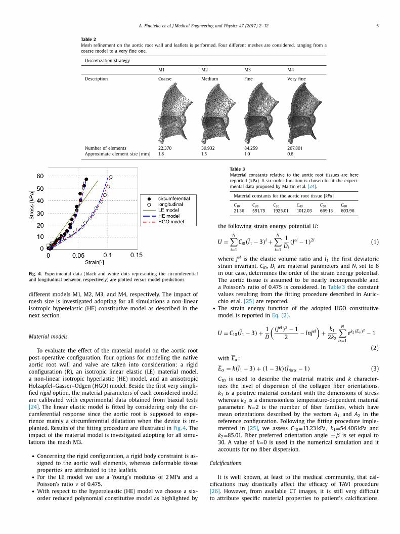
Fig. 4. Experimental data (black and white dots representing the circumferential

and longitudinal behavior, respectively) are plotted versus model predictions.

d

m

i

n

M

p

a

c

a

H

fi

a

[

c

r

p

i

l

Table 3

Material constants relative to the aortic root tissues are here

reported (kPa). A six-order function is chosen to fit the experi-

mental data proposed by Martin et al. [24] .

Material constants for the aortic root tissue [ kPa ]

C 10 C 20 C 30 C 40 C 50 C 60

21.36 591.75 1925.01 1012.03 669.13 603.96

C

c

[

t

ifferent models M1, M2, M3, and M4, respectively. The impact of

esh size is investigated adopting for all simulations a non-linear

sotropic hyperelastic (HE) constitutive model as described in the

ext section.

aterial models

To evaluate the effect of the material model on the aortic root

ost-operative configuration, four options for modeling the native

ortic root wall and valve are taken into consideration: a rigid

onfiguration (R), an isotropic linear elastic (LE) material model,

non-linear isotropic hyperlastic (HE) model, and an anisotropic

olzapfel–Gasser–Odgen (HGO) model. Beside the first very simpli-

ed rigid option, the material parameters of each considered model

re calibrated with experimental data obtained from biaxial tests

24] . The linear elastic model is fitted by considering only the cir-

umferential response since the aortic root is supposed to expe-

ience mainly a circumferential dilatation when the device is im-

lanted. Results of the fitting procedure are illustrated in Fig. 4 . The

mpact of the material model is investigated adopting for all simu-

ations the mesh M3.

• Concerning the rigid configuration, a rigid body constraint is as-

signed to the aortic wall elements, whereas deformable tissue

properties are attributed to the leaflets. • For the LE model we use a Young’s modulus of 2 MPa and a

Poisson’s ratio ν of 0.475. • With respect to the hypereleastic (HE) model we choose a six-

order reduced polynomial constitutive model as highlighted by

the following strain energy potential U :

U =

N ∑

i =1

C i 0 ( I 1 − 3) i +

N ∑

i =1

1

D i

(J el − 1) 2 i (1)

where J el is the elastic volume ratio and I 1 the first deviatoric

strain invariant. C i 0 , D i are material parameters and N , set to 6

in our case, determines the order of the strain energy potential.

The aortic tissue is assumed to be nearly incompressible and

a Poisson’s ratio of 0.475 is considered. In Table 3 the constant

values resulting from the fitting procedure described in Auric-

chio et al. [25] are reported. • The strain energy function of the adopted HGO constitutive

model is reported in Eq. (2) .

U = C 10 ( I 1 − 3) +

1

D

((J el ) 2 − 1

2

− lnJ el )

+

k 1 2 k 2

N ∑

α=1

e k 2 ( E α ) 2 − 1

(2)

with E α:

E α = k ( I 1 − 3) + (1 − 3 k )( I 4 αα − 1) (3)

C 10 is used to describe the material matrix and k character-

izes the level of dispersion of the collagen fiber orientations.

k 1 is a positive material constant with the dimensions of stress

whereas k 2 is a dimensionless temperature-dependent material

parameter. N = 2 is the number of fiber families, which have

mean orientations described by the vectors A 1 and A 2 in the

reference configuration. Following the fitting procedure imple-

mented in [25] , we assess C 10 = 13.23 kPa , k 1 = 54.406 kPa and

k 2 = 85.01. Fiber preferred orientation angle ±β is set equal to

30. A value of k = 0 is used in the numerical simulation and it

accounts for no fiber dispersion.

alcifications

It is well known, at least to the medical community, that cal-

ifications may drastically affect the efficacy of TAVI procedure

26] . However, from available CT images, it is still very difficult

o attribute specific material properties to patient’s calcifications.

6 A. Finotello et al. / Medical Engineering and Physics 47 (2017) 2–12

Fig. 5. Measurements of the real device delivery: (a) depth of implantation and (b) implantation angle.

Fig. 6. Measurements are taken considering three characteristic planes at three dif-

ferent levels L1, L2 and L3.

2

M

n

s

W

t

i

a

t

v

t

f

t

Therefore, we consider three different cases: in the first case we

simply neglect calcifications (named NC in the following); in the

second case we assign linear elastic properties E = 10 MPa and

ν = 0 . 35 (C_10 MPa) [9] ; in the third case we assign again linear

elastic properties but modeling a much stiffer material reproduc-

ing hydroxiepatite behavior (C_60 GPa). In particular, the following

parameters have been used: E = 60 GPa and ν = 0 . 3 , as reported in

Wang et al. [27] . In the two last cases, a semi-automatic gradient-

based level set method with threshold initialization, implemented

in the VMTK ( www.vmtk.org ) library, is employed to recognize the

calcific blocks (Hounsfield Units > 900). A fine mesh of approxi-

mately 50,0 0 0 linear tetrahedral elements (C3D4) for all the calci-

fications is used. By means of a kinematic coupling constraint tech-

nique, interaction between calcific blocks and leaflets is defined. A

frictionless general contact is used to handle the interactions be-

tween calcifications and the aortic root inner surface.

2.3. Positioning strategy from angiographic images

Morganti et al. [19] demonstrated that the prosthesis position-

ing has noteworthy effects on post-operative outcomes. For this

reason, Synedra View Personal 3.4 (Synedra Information Tech-

nologies, Innsbruck, Austria) is employed to analyze the intra-

operative angiographic images performed during the intervention

in order to extract the real depth of implantation d , i.e. the dis-

tance of the distal margin of the stent from the aortic annulus (see

Fig. 5 a), and the tilt angle of the device relative to the root axis

ϕ. Since it is not trivial to define the axis of the aortic root from

angiographies, as illustrated in Fig. 5 b, the ϕ angle is calculated

starting from the ϑ angle formed by the longitudinal axis of the

device and the straight line representing the aortic annulus. The

following values were obtained: d = 4 . 7 mm and ϕ = 3 . 2 deg and

considered for stent placement simulation. We neglect the pres-

sure gradients since, in the clinical practice, rapid pacing is applied

during implant deployment.

2.4. Simulation details

Following the real procedure, the stent release simulation re-

produces the progressive expansion of the device due to the pro-

gressive sliding from the bottom to the top of the constraining

catheter. Nodes at the bottom side of the stent are constrained to

prevent longitudinal translations of the prosthetic device. Self gen-

eral contact is defined for the stent. Frictionless contact is defined

to model the interaction between the inner surface of the sliding

catheter and the stent as well as the outer surface of the stent

and all valvular structures. The time-period of the device expan-

sion analysis is set to 0.4 s. A semi-automatic mass-scaling strategy

is used to speed up the analysis. During the entire simulation, ki-

netic energy is monitored to ensure that the ratio of kinetic energy

to internal energy remains less than 10%.

.5. Comparison with post-operative CT

Post-operative CT of the patient is performed on a Siemens

edCom Volume (0.4238/0.4238 pixel spacing; 3 mm slice thick-

ess). VMTK open-source software is used to extract a 3D repre-

entation of the implanted stent after processing DICOM images.

e register each resulting deformed stent surface coming from

he simulation and compare it to the real reconstructed one us-

ng the Iterative Closest Point algorithm [28] . Different quantitative

nalyses are then performed to evaluate the reliability of simula-

ion results. Only the stent is considered for two reasons: (i) the

alve is not visible from CT images, (ii) we reasonably assume that

he stent governs the post-operative performance of the valve. The

ollowing quantities are thus computed to evaluate differences be-

ween the measured patient outcome and the simulations:

• Distance map . By means of the VMTK tool, the distance be-

tween corresponding points of the two stent surfaces, i.e., the

implanted and simulated ones, is computed. • Mean distance . On cross-sections at three different characteris-

tic levels (L1, L2, L3 as shown in Fig. 6 ). Matlab software is used

for this purpose: the centerline of the stent structure is built;

then the three planes associated with the transversal section

are identified and the nodes lying on those planes are selected

and fitted with ellipses. For each of the three levels, the mean

distance between the ellipse corresponding to the simulated

stent and the ellipse related to the extracted one is calculated. • Stent eccentricity. Eccentricity of the stents is measured at levels

L1, L2, and L3. The adopted formula reads: e = c/a where c and

a are the major and the minor axis, respectively. For each plane,

the differences between eccentricities of the simulated and the

extracted stents are investigated.

A. Finotello et al. / Medical Engineering and Physics 47 (2017) 2–12 7

Fig. 7. Computational times required to complete each different simulation using

12 CPUs.

Table 4

Mean distance results, from the real extracted

stent to the simulated ones, are reported.

Mean Distance [ mm ]

Level L1 Level L2 Level L3

NC 0.7 1.45 1.2

C_10 MPa 0.6 1.1 1.1

C_60 GPa 1.15 1.4 1.6

d

a

u

3

d

s

t

i

m

A

1

3

p

(

F

s

o

m

t

Table 5

Mean distance results for each one of the

four stents are reported.

Mean Distance [ mm ]

Level L1 Level L2 Level L3

M1 4.9 3.3 2.2

M2 0.7 1.0 1.1

M3 0.6 1.1 1.1

M4 0.55 1.1 1.1

t

I

t

a

3

i

a

s

t

s

3

d

t

s

e

d

p

t

3

f

t

t

c

e

b

h

σ

o

k

e

s

m

3

a

s

u

i

p

3

e

t

Remark. Stent eccentricity measure should be considered very

carefully when checking the agreement of a simulation result

with the real configuration. In fact, if we consider two identical

ellipses lying on a plane and rotated by π /2, they present the

same eccentricity, though they are representing very different

results. In any case, circularity and axial symmetry of the device

(given by the eccentricity measure) is a very important param-

eter to predict the quality of postoperative coaptation and, thus,

prosthesis performance.

Finally, the Von–Mises stress pattern on the aortic root wall

ue to the interaction with the expanded device is also measured

nd considered for comparative purposes among the different sim-

lated cases.

. Results

The quantities computed to describe stent deformation (i.e.,

istance map, mean distance, and stent eccentricity) as well as

tress distributions on the aortic root wall are reported in this sec-

ion with the aim of highlighting the impact of different model-

ng strategies of the aortic valve complex in terms of calcifications,

esh size, and adopted material model on simulation outcomes.

ll the simulations are performed using Abaqus Explicit solver on

2 CPUs. Total CPU time of each simulation is reported in Fig. 7 .

.1. Presence of calcifications

In order to assess whether the calcifications effectively im-

act on the configuration of the deployed stent, three situations

namely NC, C_10 MPa, and C_60 GPa) are analyzed and compared.

or each configuration, the 3D reconstruction of the post-operative

tent is registered and compared with the computer simulation

utcome (see Fig. 8 ).

In Table 4 , the mean distances between simulated and extracted

odels for the levels L1, L2, and L3 are reported.

Eccentricity values are reported in Fig. 9 .

The deformed geometries of the aortic root wall obtained from

he three different simulations are plotted in Fig. 10 , providing the

ensional state of the aortic wall. Color scale shows stress in MPa.

t should be noted that the calcified blocks cause stress concentra-

ions on the aortic wall at the level of the sinuses (see Fig. 10 (b)

nd (c)).

.2. Simulation results varying aortic root mesh

We then evaluate the deployment of a Corevalve size 29, vary-

ng the adopted strategy to discretize the patient’s aortic root wall

nd leaflets. The final stent configurations at the end of the expan-

ion simulation are investigated in comparison with the shape of

he real implanted device (named “real”). Moreover, the different

tress patterns are computed and represented.

.2.1. Deformed configuration of the deployed stent

The deformed geometries of the stents obtained from the four

ifferent simulations are represented in Fig. 11 : the distribution of

he point-wise distance, from the real implanted device to each

imulated configuration, is shown.

As reported in Table 5 , mean distance for all the models and for

ach one of the three characteristic levels (L1, L2, L3) is computed.

We also measured eccentricities of the ellipses. The bar graphs

epicted in Fig. 12 show the comparison between the real im-

lanted device eccentricity and the measurements computed on

he virtually deployed stents.

.2.2. Von–Mises stress on the aortic root

In Fig. 13 , the results of the stent placement for the four dif-

erent models are reported in terms of Von–Mises stress distribu-

ion on the native aortic root wall. These results are referred to

he last frame of the expansion step. For each one of the four final

onfigurations, the average value of the Von–Mises stress of the

lements is also determined. To avoid the results being affected

y isolated peaks of stress, we exclude the 1% of the volume with

igher stress values, and we evaluate the average Von–Mises stress

M

of the remaining elements discretizing the 99 percentile of the

riginal aortic root volume. The obtained results are: σ M1 = 17.2

Pa , σ M2 = 14.8 kPa , σ M3 = 13.2 kPa and σ M4 = 13.06 kPa for mod-

ls M1, M2, M3 and M4, respectively. In Fig. 14 the resulted mean

tresses are then plotted against the normalized index representing

esh size.

.3. Simulation results varying native root material model

We evaluate the deployment of a Corevalve size 29 varying the

dopted strategy for the material model of the patient’s aortic tis-

ue. The final stent configurations at the end of the expansion sim-

lation are investigated in comparison with the shape of the real

mplanted device. Moreover, the different stress patterns are com-

uted and represented.

.3.1. Final configuration of the deployed stent

Taking the stent extracted from the post-operative CT as refer-

nce surface, the stent surfaces resulting at the end of the implan-

ation simulations are superimposed to the reference one and the

8 A. Finotello et al. / Medical Engineering and Physics 47 (2017) 2–12

Fig. 8. Distance map between post-operative real configuration and simulated ones: (a) NC, (b) C_10 MPa, (c) C_60 GPa. Minimum and maximum values are set to 0.0 and

3.0 mm, respectively; black-colored areas are related to higher values.

Fig. 9. Differences between eccentricities, at levels L1, L2, and L3 are shown.

Table 6

Mean distance between real implanted stent

and simulated one for all considered mate-

rial models, measured at levels L1, L2 and L3.

Mean Distance [ mm ]

Level L1 Level L2 Level L3

R 2.5 1.6 1.8

LE 0.35 0.8 0.8

HE 0.6 1.1 1.1

HGO 0.6 1.1 1.2

m

3

C

b

v

m

contour plot of their relative distance is computed. In Fig. 15 the

distribution of the pointwise distance to the real implanted device

in the R, LE, HE and HGO cases is shown.

Fig. 10. Von–Mises stress distribution on the aortic root wall: (a) NC; (b) C

In Table 6 , results concerning mean distances for all the tested

aterial models are provided.

Bar plots of the eccentricities are finally reported in Fig. 16 .

.3.2. Von–Mises stress on the aortic root.

Von–Mises stress distribution on the aortic wall after the

orevalve stent deployment is represented in Fig. 17 . As shown,

oth the HE and the HGO material models lead to reduced stress

alues on the aortic root wall with respect to the LE material

odel.

_10 MPa; (c) C_60 GPa; Color scale shows stress distribution in MPa.

A. Finotello et al. / Medical Engineering and Physics 47 (2017) 2–12 9

Fig. 11. Contour plot of the relative distance between the real implanted stent and the simulated one; (a) M1; (b) M2; (c) M3; (d) M4.

Fig. 12. Differences between eccentricities are shown in the bar graph for the three

levels L1, L2, L3.

4

d

g

q

a

Fig. 14. Von–Mises stress plotted against the number of mesh elements. The num-

bers of elements are normalized by the value of the elements number of the finest

mesh. Stress values are reported in kPa units.

e

p

b

j

fi

w

e

F

T

. Discussion

Transcatheter aortic valve implantation is becoming the stan-

ard procedure to resolve aortic stenosis in high-risk patients. The

rowing success of this minimally invasive technique has conse-

uently attracted the interests of many researchers who developed

dvanced computational models potentially able to support preop-

ig. 13. The analysis results show the Von–Mises stress distribution on the aortic root w

he values are calculated in MPa and the same color scale is used for all the images.

rative planning. Currently, in fact, there still occur a number of

ossible complications (ranging from paravalvular leakage to left

undle branch impairment, valve migration, or even ventriculoartic

unction rupture), which strictly depend on the native valve con-

guration (i.e., dimension, geometry, extension of calcifications), as

ell as on the device choice and adopted implantation strategy.

In this context, computer-based simulations represent a pow-

rful tool that can provide ambitious predictive information

all. Figures from (a) to (d) refer, respectively, to the models M1, M2, M3 and M4.

10 A. Finotello et al. / Medical Engineering and Physics 47 (2017) 2–12

Fig. 15. Contour plot of the relative distance is shown: (a) R model; (b) LE model; (c) HE model; (d) HGO model.

Fig. 16. Bar plot showing differences between eccentricities.

t

h

o

c

t

s

t

c

t

d

a

i

r

t

o

a

t

a

a

a

p

p

p

c

c

driving the surgeon during the decision-making and procedure

planning process. For this reason, in the last decade, many contri-

butions have been published on this topic. However, when model-

ing such a complex procedure, some analysis ingredients are not

“a priori” fixed or known and can only be assumed, either be-

cause they are almost impossible to measure (e.g., biological tis-

sue mechanical parameters), or because they are computational

parameters (e.g., discretization size). It is very well known that

Fig. 17. Von–Mises stress distribution on the aortic root wall induced by stent exp

hese parameters can drastically affect the simulation outcome;

owever, it is not still clear and consolidated what is the measure

f such an impact and how different modeling choices can really

hange clinical indications. Indeed, the aim of the present work is

o shed some light on these modeling aspects, to support future

tudies in the context of personalized medicine based on compu-

ational predictions for TAVI.

As depicted in Fig. 1 , there are some analysis ingredients that

an be reasonably assumed as known (e.g., geometric and ma-

erial details of the device to implant), and others that really

epend on specific modeling choices. In particular, beside the

ortic root geometry that can be accurately extracted from CT

mages using standard techniques, there are some modeling pa-

ameters that are arbitrary. In this paper, we focus on the three of

hem that in our opinion can more significantly affect simulation

utcomes: (i) Valve calcifications, (ii) biological tissue parameters

nd models, (iii) aortic root discretization strategy. Regarding pros-

hesis implantation site, it has been already demonstrated that it

ffects simulation results [19] . However, in this work, we do not

im at predicting postoperative performance to support preoper-

tive planning, and therefore we assume to know the device im-

lantation position from available angiographic images. This made

ossible to compare simulation results with a “ground truth” from

ostoperative CT images.

Von–Mises stress distribution on the aortic root wall is also

onsidered as an important outcome of the simulation since it

an be associated to parameters of medical interest, like the risk

ansion is shown: (a) R; (b) LE; (c) HE; (d) HGO. Stress are expressed in MPa.

A. Finotello et al. / Medical Engineering and Physics 47 (2017) 2–12 11

o

a

s

i

a

t

i

t

o

p

t

b

d

s

r

s

i

i

e

p

[

t

w

e

v

c

c

(

s

fi

t

t

i

c

w

t

i

g

r

m

o

i

m

l

r

l

p

(

s

f

t

s

s

l

t

t

c

t

m

v

p

i

t

F

t

i

s

e

o

v

t

(

m

e

a

v

o

t

s

o

t

r

t

c

b

d

v

l

n

t

(

fi

o

m

v

e

t

1

a

a

5

u

p

H

s

i

i

b

c

p

p

t

u

6

C

E

o

f triggering inflammatory processes or annulus injuries, as well

s the risk of conduction branches impairment [15,29] . In fact,

tresses induced on the aortic wall are analysed in numerous stud-

es [9,15,30] . Of course, the obtained solutions are related to the

dopted constitutive model and no exact or reference stress solu-

ions are available. Thus, we can only assess a comparative compar-

son highlighting the impact of the constitutive modeling choice on

he stress solution, which is the aim of the proposed stress results.

The presence of calcifications is unequivocally recognized as

ne of the most important factors determining (satisfactory or

oor) postoperative results. We aimed at investigating not only

he impact of modeling (or not) calcifications (which has already

een faced by Russ et al. [18] ) but we also tried to verify whether

ifferent plaque stiffness assumptions significantly alter the re-

ults or not. CT images can give information about the geomet-

ic extension of calcifications as well as about the density of the

canned materials. However, with current machine resolution, it

s difficult to classify calcifications in terms of density and almost

mpossible to obtain reliable indications about their material prop-

rties. We thus choose to model calcium taking very different

roperties from the literature (E = 10 MPa [9] and E = 60 GPa

27] ) and analyze the obtained simulation outcomes. We observe

hat, if we do not include calcifications in the native valve model,

e obtain a less deformed stent configuration (see, for example,

ccentricity measures very close to 1 in Fig. 9 ) suggesting better

alve performance than in the real case. This is expected since cal-

ifications are responsible of local device deformation affecting cir-

ularity and, consequently, valve coaptation. The distance measure

between really and virtually implanted stent) highlighted quite

ignificant differences in three regions of the device, as also con-

rmed by the mean distance measures reported in Table 4 . Varying

he material properties of calcifications also significantly impact on

he results: Fig. 8 (c) shows that using very stiff material properties

nduces even greater variance from the real solution than the “no

alcifications” case, while Fig. 9 is highlighting comparable results

ith the other simulated cases in terms of stent eccentricity at the

hree considered levels. The stress pattern on the aortic root wall

s highly influenced by calcification modeling choices ( Fig. 10 ), sug-

esting that, if the aim is to evaluate either the damage or even

upture of the aortic annulus, or the triggering of possible inflam-

atory processes within the aortic root, as well as the impairment

f the cardiac electric bundles, particular attention should be paid

n the modeling of calcifications.

As calcific plaque mechanical characteristics, also aortic root

aterial properties are unknown for patient-specific cases. Histo-

ogical evidences show that, similarly to large arteries, the aortic

oot tissue has a three-layered structure, mainly composed by col-

agen fibers embedded in a ground matrix, consisting of elastin,

roteoglycans, and water [31] . However, mechanical characteristics

stiffness, orientation, proportion of constituents, etc...) of the tis-

ue vary from patient to patient and are usually not measurable

or patients undergoing TAVI. In the present work, we aim at bet-

er understanding how different constitutive models affect the re-

ults. Four modeling strategies have been analyzed (from a very

imple rigid material to a much more complex hyperelastic non-

inear anisotropic one), all fitted to the same human experimental

ensile data.

As expected, we found that simulation outcomes are sensitive

o the aortic root constitutive model and parameters. The simplest

hoice of considering the aortic wall rigid leads to very unrealis-

ic results of an overdeformed stent, i.e., eccentricity measure not

easurable at all the levels and poor distance -between real and

irtual device- map due to the very distorted shape of the im-

lanted device (see Figs. 16 (a) and 15 (a)). Fig. 16 shows that ax-

al symmetry of the implanted device is almost everywhere main-

ained, independently from the adopted material model. Indeed,

ig. 15 seems to suggest that it is not true that more complex ma-

erial models (i.e., HGO) lead to more accurate results. Therefore

t is unuseful to adopt very complex constitutive models to repre-

ent the behavior of biological tissues, if they are calibrated using

xperimental data from the literature that are non representative

f the specific patient. Being always impossible to know in ad-

ance the peculiar properties of a specific patient, a possible solu-

ion consists in grouping patients with respect to different factors

age, sex, lifestyle, presence of genetic disesase, etc...) and deter-

ine material parameters on a statistical basis. The same consid-

rations can be drawn for stresses, that obviously depend on the

dopted material model. However, if, on one side, specific stress

alues differ from model to model (see Fig. 17 (b)–(d)), the location

f high-stress concentrations can be identified, independently from

he adopted model.

Finally, in dealing with the discretization strategy, if, on one

ide, it is recognized that the finer the mesh, the more accurate the

btained results, on the other side, it is not established which is

he threshold between reliable clinical indications (from simulation

esults) and mesh size. Fixing the material model, we then studied

he impact of aortic root mesh size on the simulation results. Very

oarse meshes, as expected, lead to very poor results, as confirmed

y Figs. 11 (a) and 12 (a). If the main interest is focused on the pre-

iction of the final stent configuration (from which the main de-

ice performance parameters depend), there exists a threshold be-

ow which inaccurate results are obtained, but also above which

egligible differences in terms of solution behavior are attained. In

he case under investigation, such a threshold corresponds to M3

mesh size in the order of 10 5 elements).

Considering M2, M3, and M4, it can be found that mesh re-

nement has a larger effect on stress values rather than on the

verall deformation of the stent. More specifically, eccentricity and

ean distance values for the stents of models M2, M3 and M4 are

ery similar (see Fig. 12 ), whereas an increase of 11,8% in the av-

rage stress is observed between M2 and M4 (see Fig. 14 ). By con-

rast, the difference between the mesh M3 and the finest mesh is

,1%. Therefore, our results show that mesh M3 can be appropri-

tely used for our purposes offering a good compromise between

ccuracy requirements and computational time.

. Conclusions

Recent studies have shown that advanced computational sim-

lations can represent powerful and helpful tools able to sup-

ort interventional cardiologists during TAVI procedure planning.

owever, each study relies on specific assumptions and modeling

trategies. In the present paper, we have focused on those that

n our opinion represent the most arbitrary choices, all regard-

ng the native pathological aortic root of the patient. The aim has

een thus to identify the trade-off between model complexity and

linical reliability of the obtained numerical results. Indications for

roper modeling the TAVI procedure have been provided. The im-

act of different calcification modeling strategies, aortic tissue ma-

erial modeling approaches, and discretization choices on the sim-

lation results of medical interest has been investigated.

. Declarations

ompeting interests

None declared

thical Approval

The patient-specific CT scan data on which the computer model

f the native aortic root was part of a retrospective clinical study,

12 A. Finotello et al. / Medical Engineering and Physics 47 (2017) 2–12

[

[

[

[

[

which was carried out in accordance with institutional guidelines.

The patient gave written informed consent prior to each examina-

tion he/she underwent.

Aknowledgments

The work has been partially supported by iCardioCloud project

by Cariplo Foundation (No. 2013–1779 ) and Lombardy Region (No.

42938382; No. 46554874).

The authors would also acknowledge Dr Anna Ferrara, Dept.

of Civil Engineering and Architecture, University of Pavia, Italy,

for providing the calibration data of the aortic tissues, and Dr

Francesco Bedogni and Dr Nedy Brambilla, Dept. of Cardiology, IR-

CCS Pol. S. Donato, S. Donato Milanese, Milan, Italy, for providing

the clinical case.

References

[1] Grimard BH , Larson JM . Aortic stenosis: diagnosis and treatment. Am Fam Phys2008;78(6):717–24 .

[2] Leon MB , Smith CR , Mack M , Miller DC , Moses JW , Svensson LG , et al. Tran-scatheter aortic-valve implantation for aortic stenosis in patients who cannot

undergo surgery. New Engl J Med 2010;363(17):1597–607 . [3] Grunau GL , Blanke P , Leipsic J . Clinical aspects and current evidence base for

transcatheter aortic valve implantation. J Thorac Imag 2015;30(6):341–8 .

[4] Neragi-Miandoab S , Michler RE . A review of most relevant complications oftranscatheter aortic valve implantation. ISRN Cardiol 2013;2013 .

[5] Koos R , Mahnken AH , Dohmen G , Brehmer K , Günther RW , Autschbach R ,et al. Association of aortic valve calcification severity with the degree of aor-

tic regurgitation after transcatheter aortic valve implantation. Int J Cardiol2011;150(2):142–5 .

[6] Vy P , Auffret V , Badel P , Rochette M , Le Breton H , Haigron P , et al. Review

of patient-specific simulations of transcatheter aortic valve implantation. Int JAdv Eng Sci Appl Math 2016;8(1):2–24 .

[7] Dwyer HA , Matthews PB , Azadani A , Jaussaud N , Ge L , Guy TS , et al. Compu-tational fluid dynamics simulation of transcatheter aortic valve degeneration.

Interact Cardiovasc Thorac Surg 2009;9(2):301–8 . [8] Sirois E , Wang Q , Sun W . Fluid simulation of a transcatheter aortic

valve deployment into a patient-specific aortic root. Cardiovas Eng Technol

2011;2(3):186–95 . [9] Capelli C , Bosi GM , Cerri E , Nordmeyer J , Odenwald T , Bonhoeffer P , et al. Pa-

tient-specific simulations of transcatheter aortic valve stent implantation. MedBiol Eng Comput 2012;50(2):183–92 .

[10] Gessat M , Hopf R , Pollok TC , Frauenfelder T , Sundermann SH , et al. Im-age-based mechanical analysis of stent deformation: concept and exem-

plary implementation for aortic valve stents. IEEE Trans Biomed Eng2014;61(1):4–15 .

[11] Tzamtzis S , Viquerat J , Yap J , Mullen MJ , Burriesci G . Numerical analysis

of the radial force produced by the Medtronic-Corevalve and Edwards–S-apien after transcatheter aortic valve implantation (TAVI). Med Eng Phys

2013;35(1):125–30 . [12] Auricchio F , Conti M , Morganti S , Reali A . Simulation of transcatheter aortic

valve implantation: a patient-specific finite element approach. Comput Meth-ods Biomech Biomed Eng 2014;17.12:1347–57 .

[13] Morganti S , Conti M , Aiello M , Valentini A , Mazzola A , Reali A , et al. Simula-

tion of transcatheter aortic valve implantation through patient-specific finiteelement analysis: two clinical cases. J Biomech 2014;47(11):2547–55 .

[14] Sturla F , Ronzoni M , Vitali M , Dimasi A , Vismara R , Preston-Maher G ,et al. Impact of different aortic valve calcification patterns on the outcome

of transcatheter aortic valve implantation: a finite element study. J Biomech2016;49(12):2520–30 .

[15] Wang Q , Kodali S , Primiano C , Sun W . Simulations of transcatheter aor-tic valve implantation: implications for aortic root rupture. Biomech Model

Mechanobiol 2015;14(1):29–38 . [16] Bosmans B , Famaey N , Verhoelst E , Bosmans J , Vander Sloten J . A validated

methodology for patient specific computational modeling of self-expandable

transcatheter aortic valve implantation. J Biomech 2016;49(13):2824–30 . [17] Grbic S , Mansi T , Ionasec R , Voigt I , Houle H , John M , et al. Image-based com-

putational models for TAVI planning: from CT images to implant deployment.In: International conference on medical image computing and computer-as-

sisted intervention. Springer; 2013. p. 395–402 . [18] Russ C , Hopf R , Hirsch S , Sündermann S , Falk V , Székely G , et al. Simulation

of transcatheter aortic valve implantation under consideration of leaflet calci-

fication. In: Proceedings of 35th IEEE Annual International Conference of theEngineering in Medicine and Biology Society (EMBC). IEEE; 2013. p. 711–14 .

[19] Morganti S , Brambilla N , Petronio A , Reali A , Bedogni F , Auricchio F .Prediction of patient-specific post-operative outcomes of TAVI procedure:

the impact of the positioning strategy on valve performance. J Biomech2016;49(12):2513–19 .

[20] Schultz C , Rodríguez-Olivares R , Bosmans J , Lefèvre T , De Santis G , Bruining N ,

et al. Patient-specific image-based computer simulation for theprediction ofvalve morphology and calcium displacement after tavi with the medtronic

corevalve and the Edwards Sapien valve. EuroIntervention 2016;11(9):1044–52 .[21] Auricchio F , Ferrara A , Lanzarone E , Morganti S , Totaro P . A regression method

based on non-invasive clinical data to predict the mechanical behavior of as-cending aorta aneurysmal tissue regression method based on non-invasive

clinical data to predict the mechanical behavior of ascending aorta aneurys-

mal tissue. IEEE Trans Biomed Eng 2016 . 22] Hopf R , Gessat M , Falk V , Mazza E . Reconstruction of stent induced loading

forces on the aortic valve complex. ProcMICCAI-Stent 2012;12:104–11 . 23] Auricchio F , Taylor RL . Shape-memory alloys: modelling and numerical simu-

lations of the finite-strain superelastic behavior. Comput Methods Appl MechEng 1997;143(1–2):175–94 .

[24] Martin C , Pham T , Sun W . Significant differences in the material properties

between aged human and porcine aortic tissues. Eur J Cardio-Thorac Surg2011;40(1):28–34 .

25] Auricchio F , Ferrara A , Morganti S . Comparison and critical analysis of invari-ant-based models with respect to their ability in fitting human aortic valve

data. Ann Solid Struct Mech 2012;4.1–2:1–14 . [26] John D , Buellesfeld L , Yuecel S , Mueller R , Latsios G , Beucher H , et al. Cor-

relation of device landing zone calcification and acute procedural success in

patients undergoing transcatheter aortic valve implantations with the self-ex-panding corevalve prosthesis. JACC: Cardiovasc Interv 2010;3(2):233–43 .

[27] Wang Q , Sirois E , Sun W . Patient-specific modeling of biomechanical interac-tion in transcatheter aortic valve deployment. J Biomech 2012;45(11):1965–71 .

28] Besl PJ , McKay ND . Method for registration of 3-D shapes. In: Robotics-DL ten-tative. International Society for Optics and Photonics; 1992. p. 586–606 .

29] Hunter R , Liu Y , Lu Y , Wang W , Schilling R . Left atrial wall stress distributionand its relationship to electrophysiologic remodelling in patients with persis-

tent atrial fibrillation. Europace 2011;13:NP . suppl. 3.

[30] Gunning PS , Vaughan TJ , McNamara LM . Simulation of self expanding tran-scatheter aortic valve in a realistic aortic root: implications of deployment ge-

ometry on leaflet deformation. Ann Biomed Eng 2014;42(9):1989–2001 . [31] Gasser TC , Ogden RW , Holzapfel GA . Hyperelastic modelling of arterial layers

with distributed collagen fibre orientations. J R Soc Interface 2006;3(6):15–35 .