MEDIA STRATEGY AND EXPOSURE ESTIMATION

"Good advertising gets attention, and its message lasts long enough through a few exposures to make one or two points. Optimally, these exposures should reach the target audience with an effective balance of a few exposures to most persons in the audience, rather than one exposure to many and many exposures to a few.

—Herbert Krugman Advertising Researcher

The minimum information which advertising management requires for decision making about advertising

alternatives involves the number of people who might see or hear the advertising and the number of times these people might see or hear the advertising. Any estimate of the impact which an advertising alternative might possibly have on sales and profits must necessarily stem from the very basic knowledge of the number of people who can be expected to be exposed to the vehicle containing that advertising. Any estímate of advertising effect on intermedíate criteria (cognitive and affective dimensions of effectiveness) must also necessarily be based upon a knowledge of the number of people exposed to the carrying vehicle. It can be said, therefore, that reach and frequency are the core, basic and fundamental concepts necessary to the effective management of advertising alternatives. This chapter will explore the ideas involved in the development of information about reach and frequency.

IMPORTANCE OF EXPOSURE ESTIMATION

As will be seen later in this chapter, the twin concepts of reach and frequency are but the opposite sides of a single coin. Though they are highly related to each other, the type of information for decision making which they provide is quite different. Reach is necessary information for the purpose of making estimates of the potential profitability of an advertising program. For example, suppose a target markeL consists of 1,000,000 households and advertising Alternative A will reach 15 percent of these households with the advertising message while Alternative B will reach 30 percent. This means that Alternative A is expected to yield a potential audience size (since reach means reach to the vehicle carrying the advertising and not necessarily the advertising itself) of 150,000 households and Alternative B a potential audience size of 300,000 households. Suppose this company has estimated, for the time interval involved, that 25,000 units of the brand must be sold to simply break even. The marketing and advertising managers estímate that, based on past experience, about 15 percent of the potential audience will buy the product. This wouid imply that under Alternative A, 22,500 purchases wouid result while under Alternativo B 45,000 purchases would result; clearly, on the basis of this information, Alternative B wouid be preferred. All estimates of the sales potential and profit potential of a brand due to the advertising for that brand must necessarily involve a knowledge of the reach of that advertising program. Frequency provides another type of essential information for decisión making. If the advertising manager wishes to arrive at some reliable estimate of the translation of potential audience size (reach) into actual sales (getting a figure such as the "15 percent" figure in the above example), this estimation process must rest on the determinaron of frequency as the starting point. The effect of advertising on the cognitive and affective dimensions of effectiveness is directly related to the number of exposures to the advertising which consumers receive in a given advertising campaign (though this relationship will differ dramatically from brand to brand and campaign to campaign). The cognitive and affective dimensions are related in some way to the conative dimensión (behavioral or sales dimensión). In one way or another, the effect of advertising on either sales or some intermedíate criterion begins with an understanding of the relationship of these to number of exposures or frequency of the advertising. The noted advertising researcher, Herbert Krugman, indicated the importance of reach and frequency in advertising planning as stated at the top of this chapter. He has aiso given some more specific information on the desirable frequency levéis in advertising in order to obtain the desired sales or other criterion-level results. Based upon his work with eye cameras which track the eye movement in responso to exposure to print advertising, Krugman suggested that three exposures were enough.' Others have conducted work in laboratory (artificial advertising exposure) situations as well as in fche field and concluded that three to four exposures appeared to provoke the optimal responso on selecfced intermedíate criteria.2 In his famous article entitled, "Why Three Exposures May Be Enough," Krugman asserted that the first exposure, like the first exposure to anything, was something new and dominated by the consumer reaction, "What is it?"3 The second exposure, he suggested, was characterized by the response, "What of it?" That is, having fully appreciated just what is the nature of the new

information on the first exposure, the consumer shifts to a question of whether or not the advertising has any personal relevance. Another element for the second exposure is the startied recognition response, "Ah ha, I've seen this before!" Such recognition permits the consumer to pick up where he or she had left off without the necessity of doing the "What is it?" all over again. Finally, on the third exposure, the consumer knows he or she has been through the "What is it's?" and the "What of it's?" and the third exposure then becomes a reminder, that is, if there is some consequence of the earlier evaluations yet to be fulfilled. It is aiso the beginning of withdrawai of attention from the completed task, or as Krugman puts it, of disengagement from the advertising. He further asserts that all exposures beyond the third serve the same basic function as the third:

. . . this pattern holds true for all larger numbers of exposures. That is. most people filter nr screen out TV commercials at any onc time by sfcopping at the "What is it?" response, without further personal involvement. The same person months later, and suddenly in the market for the product in question, might see and experience the 23rd exposure to the commercial as ifit u'ere the second. That is, now the viewer is able to go further into the nature of his or her reaction to the commercial—and then the 24th and probably the 25th might fínish off that sequence with no further reaction to subsequent exposures.4

Regardiess of how many exposures may be enough in a given situation (this will depend on such factors as the criterion involved, the type of product, the appeal, the audience, the media vehicles, and the exposure setting, among others), a decisión must be made as to what the appropriate number of exposures shouid be for the advertising campaign.s

USING EXPOSURE DISTRIBUTIONS Before examining various methods which can be used to estimate the extent and nature of exposure to a media schedule's vehicles, the primary purposes and uses of exposure distributions will be discussed. First, the definition of exposure distributíon will be given, followed by a discussion of the measures of media objectives which are derived from exposure distributions. Then an operational view of effective reach in relation to exposure distributions will be presented. DEFINITION OF EXPOSURE DISTRIBUTÍON

An exposure distribution in advertising media provides basic information essential to sound media planning and selection processes. The exposure distribution concept can be defined as a description of how many times (0,1, 2, 3, and so forth up to the total number of insertions in the schedule) a certain number or proportion of poople or households in the target market will see or hear the vehicle in which the advertisement will be placed. A sampie exposure distribution is shown below for a schedule consisting of six insertions:

Number of Number of Percentage of Times Exposed TM HH's TM HH's 0 4,400,000 25.1 1 3,900,000 22.3 2 2,300,000 13.1 3 1,800.000 10.3 4 2,600,000 14.8 5 1,900,000 10.9 6 600,000 3.5 Total 17,500,000 100.0%. For the above exposure distribution, notice that 4.4 million households would be expected to not be exposed at all to the schedule; this means that 25.1 percent of the target market households wouid not be reached by this particular schedule. Notice also that no one in the target market can be exposed seven or more times since the schedule oniy calis for six insertions. These insertions might all be in the same vehicle or different vehicles. Typically, however, the exposure distribution does not mix media types, for example, radio and magazines, but rather is estimated separately for each media type. This stems from the lack of uniform audience data across media types, and, in particular, the lack of duplication data across these types. In addition, due primarily to the cost difference between such types as radio and televisión, it is extremely difficult to consider one exposure to radio and televisión as equivalent. Subjective weighting of such inter-media differences is required but is not particularly desirable since these introduce an abstract dimension into exposure distributions. In general, it can be said that it is desirable to produce sepárate exposure distributions for each media type; a possible exception to

this general rule is in the área of simulation oí exposure distributions as illustrated by the Leo Burnett agency Mini-Compass system in the previous chapter.

It might be noted that quite often the exposure distributions which media planners actually use are truncated distributions. A truncated distribution is shown below for a schedule which consisted of 22 insertions in total: Number of Percentage of Times Exposed Target Market

0 22.1% 1 14.3 2 12.4 3 10.5 4 7.9 5 13.8 6+ 19.0 Total 100.0%.

Notice that "6+" above stands for all those people who were exposed six or more times to the media schedule; some individuáis or households (this is not specified above) will be exposed 7 times, 8 times, 9 times, and up to 22 times. Since many of these categories become very small as the size of insertions in the schedule increases, it is common practice to compress them into an "or more" category. This process is called truncating the distribution. Such exposure distributions as shown above must be estimated and are not actually known in any absoluto sense. Such distributions are actually "double estimations" since they are estimated from media data from such sources as SMRB which are themselves estimates of the population audiences of vehicles based upon sample data. Since no one individual knows for certain what the correct distribution in all cases actually is, there have been a variety of methods developed to estímate the distributions. They usually all provide somewhat com- parable answers although for certain types of schedules the answers can vary dramatically depending upon the method used. Most advertising agencies of any size have their own estimation methods on their computer or use a service süch as Telmar, Inc. of New York to do the estimation. The primary reason why exposure distributions must be estimated for particular combinations of media vehicles in a schedule is due to the problems of vehicle duplication. Duplication refers to the situation in which a given member of the target market is exposed to the advertisement in more than one vehicle (within-vehicle duplication) or is exposed to the advertisement more than one time within the same vehicle (between-vehicle duplication). Figure 14-la illustrates audience duplication for three vehicles where one insertion is placed in Magazine A, one in Magazine B, and one insertion in Magazine C. The center triangle is called the "triplicatíon" or third-order duplication and represents the people who are exposed to all three magazines. Área AC represents the number of people who are exposed oniy to Magazine A and Magazine C. If a fourth magazine were added to this schedule, then the fourth-order duplicated audience size wouid need to be determined. Since services such as SMRB oniy measure among their sample members the duplicated audiences between magazine pairs, any duplication of an order above two (pair-wise duplication) must, therefore, be estimated in order to produce an exposure distribution. In Figure 14-la, suppose Magazine A has an audience among the target market of 1.1 million households, Magazine B's audience is 1.3 million HH's, and Magazine C's audience is 1.4 million HH's. These total audiences are distributed across the various áreas in Figure 14-la. Notice that the unduplicated reach for one insertion in each of the three vehicles wouid be 2.9 million households and not 3.8 million (3.8 million is the sum of the individual magazine audiences and wouid be the gross reach). Reach refers to the number of uniquc individuáis exposed one or more times. This can be found by adding up each individual área in Figure 14-la to arrive at 2.9 (2.9 = .5 + .7 + .9 + .3 + .2 + .2 + .1); it can aiso be found through the application of the Inclu P. Exclusion formula (as in Boolean Algebra). The Inclusion/Exclusion Principie states that the probability of exposure to Magazine A or Magazine B or Magazine C is equal to the sum of the probabilities of '.posure to each of them minus the three pair-wise duplication probabilities (for example, as between Magazine A and Magazine B) and, really, plus the probability of triplication. Though probabilities have '. been used in this illustration, the same thinking applies: 2.9 = 3.8 4 + .3 4- .3) 4- .1. Notice, for example, that .4 is the duplication been Magazine A and Magazine B in Figure 14-la (.4 = .1 + .3). audience accumulation is aiso illustrated in Figure 14-lb for •'Jgazine A. Each circle, in this case, now represents an insertion in '.¿gazme A, so three insertions are shown for the same vehicle, .'. agazine A. The reach of three insertions in Magazine A is 2.5 million 'useholds (2.5 = .5 4- .6 4- .7 4- .3 4- .1 4- .2 4- .1); or through Boolean '-.Igebra, 2.5 = 3.3 — (.4 4- .3 4- .2) 4- .1. Accumulation, in other words, moves the duplication which takes place within a vehicle rather than . ross or betwecn vehicles (to which the term net audience is ordinarily .pplied).

When a media scheduie calla Cor insertions in aeveral vehicles and/or \ eral insertions in the same vehicle, the process of estimating the oxiuro distribution amounts to a process of removing the double 'unting, triple counting and so forth from the sum oí the individual audiences of the insertions. MEASURES DERIVED FROM EXPOSURE DISTRIBUTIONS Most of the important measures utilized in the process of selecting a -chedule in conformance with media objectives are derived from the -stimated exposure distribution. These measures include: reach, LTRP'S (gross reach, or gross impressions), average frequency, effective 'each, and various CPM (cost per thousand) measures. The derivation : f each of these important measures will be illustrated in the following ¿xample.

Example 14-1. The brand manager of Kelso detergent at the Caspen Company is faced with the problem of selecting a television media schedule to be used in the next quarter for Kelso. The cholee has been narrowed to two media scheduie alternatives. Below are the exposure distributions for the two TV media schedules: Exposure # Media #l Media #2 0 22% 30% 1 35 25 2 30 20 3 7 25 4+ 6 0 Total 100% 100%.

Figure 14-1 Audience Duplication and Accumulation for Three Magazines Vehicle Audiences: Magazine A – 1.1 million honseholds Magazine B – 1.3 million households Magazine C – 1.4 million households

(a) Audience Duplication (b) Audience Accumulation The size of Kelso's target market is estimated as 35 million HH's. Media schedule #1 above will cost a total of $155,000 while schedule #2 will cost a total of $139,000.

By applying the percentages in the above distributions to the target market size, the household distributions can be examined:

Exposure # Media #1 Media #2 0 .22 x 35 = 7.7m .30 x 35 = 10.5m 1 .35 x 35 = 12.25 .25 x 35 = 8.75 2 .30 x 35 = 10.5 .20 x 35 = 7.0 3 .07 x 35 = 2.45 .25 x 35 = 8.75

4 .06 x 35 = 2.1 .00 X 35 = 0.0 . Total 35.0m 35.0m.

Reach (unduplicated reach) can then be calculated for each schedule in a number of ways: Media # 1 Media # 2

Reach (%) 78% = 100% - 22% 70% = 100% - 30% Reach (HH’s) .78 x 35 = 27.3mHH’'s .70 x 35 = 24.5mHH's (27.3=12.25+10.5+2.45+2.1) (24.5=8.75+7.0+8.75+0). In other words, reach is the sum of those individuals reached 1 time, 2 times, 3 times and 4 times or more; this is equivalent to subtracting the number not reached (or percentage) from the total number of people in the target market (or 100%). GRP's (gross rating points) are calculated as follows as are gross reach or gross impressions (the non-percentage counterpart of GRP's): Media # 1 Media # 2GRP's 140 = (35 x 1) + (30 x 2) + (7 x 3) + (6 x 4) 140=125 X1)+(20X2)+(25X3)+(0X4) Gross Reach 140% x 35 = 49m 140% x 35 = 49m. GRP's and gross reach are measures, therefore, of the total percentage or number of exposures delivered by the media schedules; the term gross reach is sometimes called duplicated reach to indícate that the measure includes the same person or household counted more than once. Average frequency is then calculated for each schedule: Media #1 Media #2Average Frequency 140 / 78 = 1.8 140 / 70 = 2.0 (49m / 27.3m = 1.8) (49m / 24.om = 2.0). Schedule # 1 would be expected to deliver an average of 1.8 exposures to the vehicles included in the schedule while schedule # 2 would deliver an average of 2.0 exposures to the vehicles.

CPM/TM (cost per thousand to the target market) can be calculated as follows:

Media # 1 Media #2

CPM/TM ($155,000 / 27,300,000) x 1000 = $5.68 ($139,000 / 24,500,000) x 1000 = $5.67. In other words, it will cost $5.68 for every one thousand target market members reached by schedule #1 while this cost will be $5.67 for schedule #2, almost identical.

Finally, the effective reach and cost per thousand in terms of effective reach to the target market can be calculated. Suppose effective reach is defined in the manner used by the media department at the J. Walter Thompson advertising agency (as discussed in Chapter 13); this agency defines effective reach as the number of people in the target market reached between 3 and 10 times. In the current example, effective reach would be: Media # 1 Media # 2ER (%) 13% = 7% + 6% 25% = 25% + 0% ER(HH's) 4.55mm = 2.45 + 2.1 8.75mm = 8.75 + 0 CPM/TM/ER ($155,000 / 4.55mm) x 1000 = $34.06 ($139,000 / 8.75mm) x 1000 = $15.88. Clearly, in terms of this particular definition of effective reach, schedule /f2 is more cost efficient.

MESSAGE/MEDIA RESPONSE VALUES As noted in Example 14-1 above, effective reach can be defined as the number of exposures a target market individual or household receives. It might also be defined in terms of criteria higher in level (as these levels of reach were defined in Chapter 13) of reach such as in the cognitive, conative, or affective dimensions. Measures of commercial or advertisement effectiveness for the message to be used in the media schedule might be copy researched on criteria such as advertising awareness, attítude chango, or intentions-to-buy. This information couid then serve to define the meaning of "effective reach" as it is used in the media process. Only one criterion might serve in the definition of effective reach or some combination (multiple criteria) might serve in the definition. If multiple criteria are employed, however, it might be noted that the criteria wouid often be combined for decision making purposes using subjectiue weights which reflect the decision maker's attribution of importance of these criteria as indicators of commercial effectiveness. If subjective weighting is employed in the effective reach, it should be noted that an abstraction is then introduced into the reach values; the resulting reach figures shouid. accordingly, be used only in a relative sense to be compared from one media schedule to the next. An example of the calculation of Message/Media Response Valúes as an indicator of effective reach is given below. Example 14-2. This example is a continuation of that begun in Example 14-1. Suppose that Kelso's brand manager believes oniy in testing commercials on the recall measure of the awareness criterion. The distribution of correct Day-after Recall (DAR) scores for two commercials being considered for possible use in the media schedules given in Example 14-1 are shown below: Exposure # Commercial A Commercial B 0 0% 0% 1 7 8 2 15 25 3 20 20 4 24 20. As can be seen from the above, each of the two commercials has been tested over four exposures (multiple exposure copy testing) to a representative sample drawn from the target market for Kelso detergent. The following will illustrate how the four Message/Media Response Values (MMR's) are calculated for the four possible combinations of two media schedules and two commercials. For example, in the case of Media #1 and Commercial A:

HH DAR Effective

Exposure # Distribution Distribution Reach . 0 7.7mm X 0.00 = .00 1 12.25 X .07 = .86 2 10.50 X .15 = 1.58 3 2.45 X .20 = .49 4+ 2.10 X .24 = .50 MMR Value 3.43. The Message/Media Response value is the sum of the effective reach figures calculated for each level of exposure. It is, therefore, a measure indicating the expected number of households to result with correct day-after recall of Commercial A when carried in Media schedule #1. It would be expected that 3,430,000 HH's wouid be effectively reached using this particular combination of media and commercial. The MMR valúes for all four combination of schedules and commercials are given below: CPM / TM / ER Media # Commercial MMR Value (based upon MMR values)1 A 3.43 $45.19 = (155 / 3430) x 1000 1 B 4.52 $34.29 = (155 / 4520) x 1000 2 A 3.41 $40.76 = (139 / 3410) x 1000 2 B 4.20 $33.10 = (139/4200)X1000. In terms of cost efficiency based upon the effective responso defined in the MMR manner, the combination of schedule #2 and Commercial B is the best alternative. In terms of MMR values alone without regard to cost, Schedule tt\ and Commercial B wouid be superior since that combination delivers the largest number of effectively reached households, 4,520,000 compared to omy 4,200,000 for Media #1 and Commercial B.

Since the exposure distribution provides such basic and important information to the media planner, it is appropriate to examine the methods by which such distributions can be developed. The next section provides an overview and historical perspective on the development of exposure distribution models. The last section of this chapter will show by example how four of the more important methods are applied to actual problems in media.

OVERVIEW OF EXPOSURE ESTIMATION METHODS There have been many methods developed over the years since Hyett first developed the application of the Beta distribution to the problem of exposure estimation in 1958.6 It is not possible to discuss here all methods which have been developed and utilized over the past twenty-some years; at any rate, many of these methods are proprietary and nothing has been published in a public way regarding their nature. But several important, published methods will be examined to give some indication of the general nature of exposure estimation methods. These will be discussed by the following categories: (1) Ad hoc models; (2) Stochastic models; (3) Ad hoc/stochastic combination models; and (4) Simulation models. After this general discussion, the application of four useful and important methods of exposure estimation will be examined. AD HOC MODELS The methods which will be referred to here as "ad hoc" are those which have been developed with no particular rationale or "theory" purported to underlie the method. The primary criterion which the developers of ad hoc methods employ is estimation accuracy; that is, these people search for "formulas" which will accurately and reasonably reproduce actual, known reach estimates for media schedules as well as give reasonable extensions of reach for the schedules. The difficulty with such methods lies in the extent of their generalizability to "new" schedules which were not examined by the developer in the process of building the ad hoc formula. Because the method encompasses no overall theory of how the vehicle accumulation and duplication processes work, it may hold only for the peculiarities of the particular schedules analyzed by the developer or for schedules which are very similar to those schedules. It is difficult to specify the characteristics of media schedules ahead of time for which the method shouid perform well since the method is not tied explicity to theoretical assumptions about the duplication and accumulation processes it attempts to represent. With this in mind as a limitation, methods which have, nonetheless, performed quite well in actual tests can be found among the ad hoc formula-type methods. Of the four methods to be discussed here, two (Hofmans' and Morgensztern's formulas) have performed quite well on schedules for which the actual reach and exposure distributions were known. One of the earliest attempts (after Hyett mentioned above) to systematically estímate unduplicated reach was by Agostini,7 a Frenchman. In 1961, he developed the following empirical formula based upon his analysis of French magazine readership: R = A . 1 + (KD) / A where: R = the net coverage (reach) of a set of m vehicles A = the sum of the readership (audience) of each vehicle included in the set. D = the sum of the duplicated readership of all pairs of vehicles in the set. K = 1.125 (Agostini's Constant). It can easily be seen from the above that the reach (R) of one insertion in Magazine A which has an audience, for example, of 200,000 house- holds and one insertion in Magazine B which has an audience size of 300,000 households, where the duplicated audience between A and B is 50,000, wouid be calculated as 350,685 (350,685 = 400,000 / {1 + 1.125 (50,000) / 400,000}). Though the procedure suggested by Agostini produced some close estimates of reach, Claycamp and McCIelland eventually demonstrated that Agostini's constant was, in fact, a variable dependent upon the average number of vehicles read per readers and the variation of this statistic over the population.8 The development of exposure distributions is very importantly linked to this early work (from the above it can be seen that Agostini's formula oniy produces one number as a result, the total unduplicated reach for the schedule) on reach estimation. The two, reach estimation and exposure distribution estimation, are very closely linked. An exposure distribution will produce the frequencies of a certain proportion of the audience exposed no times, one time, two times, three times, and so forth. Reach can be calculated from this exposure distribution in two ways: (1) Reach can be calculated by subtracting the number of people in the zero-class or no-exposure frequency class from the total

number of people in the target market (or the proportion or percentage in the no-exposure class from 100 percent); and (2) by summing up the number or proportion of people in each of the exposure classes other than the zero-class. These two figures are equivalent if the calculations have been conducted accurately. Another ad hoc method was developed by Young to estímate the reach of radio audiences.9 Young conducted regression analysis on data for several variables obtained on a sample of 86 radio schedules. For this sample size of 86, Young found a high relationship (R2 of between .86 and .95, depending upon the demographic group analyzed) between the known reach (the dependent variable) of the 86 schedules and four independent or explanatory variables: GRP's of the schedule, number of radio stations used in the schedule, number of time periods used, and the number of spots per station. Using a modified exponential functional form, regression analysis yielded parameters of the function; this function couid then be used to estímate reach for a new schedule (not one of the 86 sample schedules used to build the function) of radio spots. One of the modeis he developed, with its appropriate parameter valúes inserted was: R = 85 { 1 – (.659)e-.51X1 -0.7X2 - .08X3 + .04X4 } where: R = proportion (percentage) reach of the schedule 85 = saturation reach (maximum coverage of stations used in schedule) e = the natural number 2.718 . . . X1 = GRP's of schedules X2 = number of stations used in schedule X3 = number of time periods used in schedule X4 = number of spots per station. For example, suppose a radio schedule calls for GRP's of 146, three stations, 1 time period (6-10 a.m.), and 24 spots per station. The reach for this schedule would be calculated as: R = 85 {1 - (.659) (2.718) -.51(1.46) – 0.7(3) – 0.8(1) - .04 (24)

R = 33.8 percent. Unfortunately, with this model as with most other ad hoc methods, no information has been provided as to the accuracy of the reach projections for actual media schedules beyond the 86 initially used to build the model's parameters as given above. And, of course, since the model was built in 1972, the parameters given above wouid not hold, in anycase, for today's situation. It shouid be noted aiso that this model was built specifically for radio schedules. Sepárate modeis wouid be needed for spot television, network television, network radio, magazines, newspapers, and so on. But this is aiso true of most exposure estimation models. One of the documented ad hoc models is that developed by Hofmans. another Frenchman, in 1966."' This model has been tested quite extensively on magazine schedules and has performed overall quite well. Hofmans' formula can be viewed as a variation of Agostini's formula where Agostini's constant has been replaced by a variable K. In Hofmans' formula, K is a function and varíes in relation to the individual audience sizes of the vehicles involved as well as the pair-wise duplications between all the vehicles in the schedule. In one large-scale test of Hofmans' formula, the formula produced an average error of 2.46 percent compared to 3.86 percent error of estimated versus actual reach of magazine schedules for Agostini's formula." A virtue of Hofmans' method is its simplicity for the degree of accuracy provided in its use. Since the application of Hofmans' method is illustrated in Appendix A to this chapter, the explanation of the model will wait until that point. Another variation of Agostini's method was developed by the Frenchman, Morgensztern in 1970 which takes into account both the duplication within and between vehicles as does the Hofmans Modified method to be applied later in this chapter. Morgensztern's model is, thus, a multi-vehicle, multi-insertion model as opposed to Agostinfs formula which can oniy be used in the multi-vehicle situation where one insertion is used in each vehicle in the schedule. Since the formula for Morgensztem's model is very similar to Hofmans' formula, it will not be given here. It can be noted, however, that on a test of 57 magazine schedules for which the actual reach was tabulated by IMS (Interactivo Market Systems, Inc. in New York), the Morgensztern model had an average percentage error in its reach projections of 2.82 percent.12 This is compared with 2.80 percent error on the same 57 schedules for the Hofmans model. The additional complicatíon introduced by Morgensztern does not appear worth the additional effort required over Hofmans' approach. STOCHASTIC MODELS Stochastic models differ from ad hoc approaches inasmuch as they require the explicit statement of hypotheses about the nature of duplication and accumulation processes underiying the development of schedule reach. Such

hypotheses can, therefore, be tested and either accepted or disregarded for tuture work and application. Stochastic models also convey the view that exposure to a media schedule is a probabilistic process and not a deterministic one; that is, it is assumed that exposure is, in some measure, a chance process. Such methods are also to be desired over most ad hoc modeis because they produce exposure distributions from which reach may be calculated whereas the foregoing ad hoc models only produce the reach estímate itself. Exposure distributions, as was pointed out at the beginning of this chapter, provide helpful decision making information which can be masked when oniy reach and average frequency are employed in this process. Most Stochastic methods are aiso based upon known mathematical probability distributions such as the binomial distribution, the hypergeometric distribution, and so forth. Use of known probability distributions has several advantages. First, a probability distribution is positive everywhere on its interval of definition so that logical errors such as negative reach figures are impossibilities; this sometimos occurs in ad hoc modeis such as Hofmans' and others. Second, the área under the probability curve of the distribution adds up to 100 percent and, therefore, illogical outcomes such as a reach greater than 100 percent are not possible; this phenomenon aiso occurs in some ad hoc procedures for certain types of schedules. And, finally, if a known probability distribution is utilized in the exposure estimation process, the way in which the "parameters" can be found is fairly well-known since mathcmaticians will have studied the distribution for a long time. As indicated earlier, Hyett developed a procedure in 1958 for estimating the cumulative coverage (reach) of a schedule based upon the Beta distribution. This important development established the procedure used in contemporary Stochastic models. In most cases, the procedure for estimating the distribution of exposures begins with the assumptíon that the pattern of exposure distribution follows one or more well-known theoretical probability distributions. Once the parameters of the theoretical distribution have been estimated from actual data using one of several methods (some of these are the method of moments, máximum likelihood methods, and least squares estimators), the complete estimated exposure distribution is generated by the theoretical distribution.

Another procedure developed in Britain for the purpose of estimating reach, as opposed to the full distribution, is the Sainsbury technique.13 The Sainsbury method assumes that exposure is a Bernoulli process (that is, that it follows a binomial distribution). The method can be stated as follows: Rm = 1 - (1 – p1) (l – p2) (l – p3) … (1 – pm) where: Rm = reach of"m" vehicles in a schedule with one insertion in each vehicle. pi = the audience of vehicle "i" expressed as a percentage of the target market size. For example, suppose three vehicles have audiences of 24 percent, 30 percent, and 20 percent. Using the Sainsbury model, reach would be 57.4 percent (.574 = 1 - {(1 - .24) (1 - .30) (1 - .20)}). In a test of the Sainsbury model on nine schedules of five magazines each and nine schedules of 11 magazines each, the average percentage error was 18.32 percent and 24.58 percent, respectively.

The Sainsbury method was modified for the case in which duplication data were available between pairs of vehicles in the schedule. In this case, the formula becomes: Rm = l - {(qd1) (qd2) (qd3) … (qdm)} where: qi = (1 - pi) or the "noncoverage of vehicle i"

dqi = qij / qj or the "adjusted noncoverage" of vehicle i by vehicle j where vehicle j is the vehicle in the schedule with the largest audience size. For example, suppose the three vehicles used above to ¡Ilústrate the Sainsbury "normal" method are in a schedule and the net coverage (unduplicated pair-wise audience) of vehicle 1 with vehicle 2 is 40 percent, vehicle 1 with vehicle 3 is 30 percent, and vehicle 2 with vehicle 3 is 45 percent. This information is summarized below: Coverage Noncoverage Vehicle 1 24% 76% Vehicle 2 30 70 Vehicle 3 20 80 Vehicles 1 & 2 40 60 Vehicles 1 & 3 30 70 Vehicles 2 & 3 45 55.

Since Vehicle 2 has the largest audience (30%), it will be used to adjust the coverages of the other vehicles. Then: qd1 = q12 / q2 = .60 / .7 = .86 qd2 = q22 / q2 = q2 = .7 qd3 = q23 / q2 = .55 / .7 = .78 and R3 = 1 - {(.86) (.70) (.78)} = 53%. Notice that by inclusion of the information on pair-wise vehicle duplication (the net audiences), the reach estímate was reduced from the 57.5 percent in the preceding example to the 53 percent figure above. In a test of the Sainsbury Modified method on the same schedules of five and 11 magazines reported above, the percentage er- ror was reduced from the 18.32 percent figure to 6.2 percent for the five-magazine schedules and from 24.58 percent to 12.69 percent for the 11-magazine schedules. Thus, the Sainsbury Modified formula is superior to the Sainsbury "normal" method. In 1964, Richard Metheringham, media director at Foote Cone & Belding advertising agency in Britain, reported his method of exposure distribution estimation which incorporated both the Beta distribution used by Hyett and the Binomial distribution which serves as the basis for the Sainsbury method.14 It is based on the compound Beta Binomial Distribution, though Metheringham himself described the method as an empirical formula (ad hoc) and thus free of any assumptions inherent in any theoretical probability distribution. The Beta distribution is used to estímate the probabilities that an individual is exposed to any one, any two, any three and up to any number of vehicles included in the schedule. These probabilities are then used in the Binomial distribution to estímate the distribution of exposures, that is, the proportion of the target audience that is exposed to one and oniy one insertion, two and oniy two insertions, and so on. The method is attractive since the oniy data required for the exposure distribution estimate are: (1) the average vehicle audience (vehicle coverage); (2) the two-insertion cumulative audience ofeach vehicle; and (3) the pair-wise duplicated audience or net audience for each combination of two vehicles. In a test of the method on the 57 IMS media schedules for magazines indicated earlier, the average percentage error of estimated versus actual schedule reach for the Metheringham method was 5.2 percent.15 This is quite excellent when compared with many other methods.

The final stochastic model to be examined in this overview is that developed by Kwerel in 1969.16 Kwerel's model is detailed and applied in Appendix A to this chapter so that it will not be discussed in detail at this point. It might be noted, however, that the reach estimates of the Kwerel model were tested on schedules of three, four, and five magazines; the percentage error in the reach estimates for these schedules were 1 percent, 3.3 percent, and 6.8 percent, respectively. When Hofmans' formula was utilized on the same schedules, the reach errors were 2 percent, 4.2 percent, and 6.0 percent, respectively.17 In general, it has been found that Hofmans' formula performs better on large schedules (those including a large number of vehicles) while Kwerel's method performs better on small schedules (those with four or fewer vehicles involved). AD HOC/STOCHASTIC COMBINATION METHODS The most recent work in the area of exposure distribution estimation shows again that the Beta Binomial Distribution (BBD) is an appropriate basis upon which to model the exposure distribution problem. Headen, Kiompmaker, and Teel developed in 1976 an interesting combination procedure for use of the BBD as a model for the problem. The method is really a combination of the approaches utilized by Young and those utilized by Metheringham described earlier in this chapter." There are three parameters which must be estimated in order to use the BBD. One of these parameters can be considered as the numer of insertions in the schedule. The remaining two must be estimated from the first two "moments" of the distribution: the mean and variance. The mean of this distribution can be represented by Gross Rating Points for televisión schedules. However. the variance is unknown and must be estimated. In this procedure, the variance is estimated as a function of four independent variables: number of insertions in the schedule, number of vehicles used in the schedule, number of vehicles available, and the average audience of the schedule's vehicles. Regression analysis on a sample of schedules is used to estímate the variance. Once this is accomplished, the parameters of the BBD can be calculated through simultaneous solution of the "moment equations" which represent the two parameters as a function of the mean and variance of the distribution. The developers have presented evidence that this procedure works quite well for both network television and spot televisión media schedules.

SIMULATION MODELS The general approach regarding the simulation of reach through exposure distributions has been examined in the preceding chapter with regard to the comprehensive media model called Mini-Compass and utilized by the Leo Burnett advertising agency. Several other simulation approaches liave been developed over the years. Greene's personal probability assignment method, which is a combination of simulation and probability distribution methods, has been examined closely for performance and is apparently quite acceptable.19 The performance of most other simulation methods, such as CAM in Britain, the SCAL model in France, and the model developed by the Simulmatics Corporation in the United States has not been well documented publicly.20 It is interesting to note the SCAL model was supplanted by the Morgensztern model discussed previously in this chapter by a number of large French advertising agencies; this has taken place because of the methodological weakness inherent in the simulation approach. Simulation of exposure distributions is not the most computationally efficient means of reach estimation to include in a comprehensive media planning and selection model, because in the optimization process the computer must sometimes examine as many as 20,000 simulated individuals’ exposure probabilities. In “formula” models, such as the ad hoc and stochastic methods discussed above, relatively fewer calculations must be made than in the simulation approach. When a comprehensive model must examine 30 or 40 different media schedules to find the best one, the number of calculations to arrive at the schedule reach in each case can become overwhelming and very time consuming even with the fastest computers. Of all the simulation approaches, the approach of Greene mentioned above is probably most desirable because of its reported accuracy and because it combines the simulation approach with the stochastic approach.

APPENDIX A SOME ESTIMATION METHODS IN APPLICATION Four methods of estimating reach will be examined in this Appendix through the use of examples: (1) Hofman’s Model; (2) Kwerel’s Model, (3) Metheringham Method (Beta Binomial Distribution); and (4) Multivariate Polya-Eggenberger Distribution (Dirichlet Multinomial Distribution). The latter two produce the complete exposure distribution. While an extension of Kwerel’s basic method will produce an exposure distribution, it will not be examined or illustrated here. The data which will serve as the basis for all computations in the examples in this section are provided below:

Hofman’s and Kwerel’s Multi-Vehicle, Single-Insertion models will be used to estimate the reach of a schedule consisting of one insertion in each of the three magazines above for a total of three insertions in the schedule. Hofman’s and Kwerel’s Multi-Vehicle, Multi-Insertion models as well as the Beta Binomial and Dirichlet Multinomial models will be used to estimate the reach of a schedule consisting of two insertions in each of the three magazines for a total of six insertions in the schedule. In addition, the complete exposure distribution will be calculated for the latter schedule using the BBD and DMD methods. Hofmans' Multi-Vehicle, Single-insertion Model (Example 14-3) In each of the examples in this section, the basic formulas for the models will be given first; then the application of the formula will be shown in a numbered, step-by-step sequence. Hofmans' basic formula is given by:

The reach of one insertion in three vehicles is, therefore, according to Hofmans' Method, 29.82 percent. Hofmans' Multi-Vehicle, Multi-Insertion Model (Example 14-4) Here it will be assumed that the multi-insertion schedule consists of two insertions in each of the three magazines indicated above for a total of six insertions in the schedule.

Fortunately, for two insertions maximum in any given vehicle, Σkd reduces to Σkidi where: ki = 2R1 / R2 d = 2R1 – R2 Ri = coverage of "i" insertions in a given vehicle.

The reach of the six-insertion schedule is 36.8 percent using Hofmans' model. Kwerel’s Multi-Vehicle, Single-Insertion Model (Example 14-5)

Rm = 2(UB) (LB) / (UB + LB)

The reach of one insertion in each of the three magazines is 30.02 percent using the Kwerel approach. Kwerel's Multi-Vehicle, Multi-Insertion Model (Example 14-6)21

A = ΣniAi : sum of the audiences for the insertions Ā = A / N: average audience where N is the total number of insertions (N=6) Σdi = Σ(n

2i) (2R1 – R2): duplication within vehicles where: (n

2i) stands for the number of combinations of ni things taken 2 at a time. In general, the number of combinations of n things taken r at a time is given by

The reach of the six-insertion schedule utilizing the extended Kwerel model is 34.87 percent. Metheringham Method (Beta Binominal Distribution) (Example 14-7) The method developed by Metheringham in 1964 is equivalent, as indicated earlier in this chapter, to the application of the Beta Binominal distribution. The calculation approach adopted by Metheringham is considerably more complex than that which is actually required to genérate the exposure distribution based upon the BBD. Though the approach shown here is different than that utilized by Metheringham, it can be shown that it produces identical results to his calculation approach; it is adopted here because of its relative simplicity.

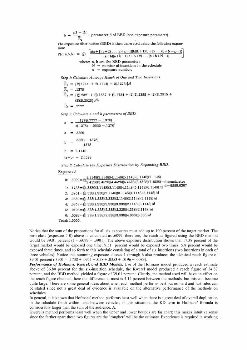
Notice that the sum of the proportions for all six exposures must add up to 100 percent of the target market. The zero-class (exposure # 0) above is calculated as .6099; therefore, the reach as figured using the BBD method would be 39.01 percent (1 - .6099 = .3901). The above exposure distribution shows that 17.38 percent of the target market would be exposed one time, 9.51 percent would be exposed two times, 5.8 percent would be exposed three times, and so forth to this schedule consisting of a total of six insertions (two insertions in each of three vehicles). Notice that summing exposure classes 1 through 6 also produces the identical reach figure of 39.01 percent (.3901 = .1738 + .0951 + .058 + .0353 + .0196 + .0083). Performance of Hofmans, Kwerel, and BBD Models. Use of the Hofmans model produced a reach estimate above of 36.80 percent for the six-insertion schedule, the Kwerel model produced a reach figure of 34.87 percent, and the BBD method yielded a figure of 39.01 percent. Clearly, the method used will have an effect on the reach figure obtained; here the difference at most is 4.14 percent between the methods, but this can become quite large. There are some general ideas about when each method performs best but no hard and fast rules can be stated since not a great deal of evidence is available on the alternative performance of the methods on schedules. In general, it is known that Hofmans' method performs least well when there is a great deal of overall duplication in the schedule (both within- and between-vehicles; in this situation, the KD term in Hofmans' formula is considerably larger than the sum of the audience, A. Kwerel's method performs least well when the upper and lower bounds are far apart; this makes intuitive sense since the farther apart these two figures are the "rougher" will be the estimate. Experience is required in working

with particular vehicles and schedules in order to "know" what "far apart" might mean in a particular situation since this is a relative idea. The Metheringham method (BBD) is known to produce a phenomenon called "declining reach" when large and extremely small audience vehicles are mixed in the same schedule. This is an illogical and impossible outcome in reality. For example, a schedule consisting of two insertions in Vehicle A (audience size of 13.5%) and two insertions in Vehicle B (audience size of .8%) where A's two-insertion cumulative audience is 24.8%, B's cumulative audience is 1.33%, and the net audience between A and B is 13.98% produces a BBD reach figure of 41.34%. However, when the four Vehicle B insertions are removed from the schedule and the BBD reach is re-estimated, the reach increases to 42.38%. This, of course, is illogical and a physical impossibility. Reach cannot decline or become smaller when insertions are added to a schedule; even if duplication of the additional insertions with those already in the schedule was 100%, the reach would remain the same and not decline. The BBD method is also known to generally overestimate the true size of the schedule reach; in the above examples, it can be noticed that the BBD reach is larger than either Hofmans or Kwerel reach. Dirichlet Multinominal Distribution (Example 14-8) One of the most recently developed approaches based upon a probability distribution utilizes the compound Dirichlet multinomial distribution (DMD).22 This distribution is a member of the family of distributions called Multivariate Polya-Eggenberger Distributions. This method overcomes the problem of declining reach often observed in conjunction with the Metheringham application of the BBD. As will be seen in the first step below of the application of this method, some ad hoc method must be used first to calculate the reach of one insertion in each of the vehicles. In this illustration, Hofmans' formula is used, but some other approach such as Kwerel's model. for example, could just as well be used in the first step. This method is also the multivariate form of the beta binomial distribution (BBD) so that it will be seen in step 4 below that the method used in Example 14-7 to fit the BED parameters "a" and "b" in steps 2 and 3 in that example are used in the DMD method here.

It might be noted that although the Metheringham method has been shown to produce acceptably accurate reach estimates (although it usually overestimates reach), the BBD distribution upon which the method is based is not capable of reproducing multiple peaks or modes of an exposure distribution. The BBD is at most a bi-modal distribution (two peaks) whereas the DMD can exhibit many peaks in the exposure distribution. This will be observed when the distribution generated below using the DMD is compared with that in Example 14-7 which used the same data as those used below. Step 1: Application of Hofmans' Multi-Vehicle, Single Insertion Formula. This formula was already used on the data for which the DMD will be used (two insertions in each of the three magazines indicated at the beginning of this appendix); the results of that application can be seen in Example 14-3. In Example 14-3, the reach of one insertion in each of the three vehicles was calculated to be .2982 or 29.82 percent. Step 2: Use of the Inclusion/Exclusion Principle to Find Sum of nth Order Duplications.

Step 3: Use Waring's Theorem to Find Exclusive Exposure Probabilities. It should be noted that, when the proportion of a vehicle's audience to the target market is viewed as a probability of exposure to that vehicle by a

member of the target market, this probability is not an exclusive exposure probability. Exclusive probabilities must sum to unity (100 percent) for all the vehicles in- volved in a media schedule. 8uppose four vehicles are considered for inclusion in a media schedule, and these vehicles have percentage audiences of .34, .29, .45, and .30. Clearly, in this case the sum of the individual audience percent- ages (exposure probabilities) exceeds 1.00 (.34 + .29 + .45 + .30 = 1.38); this is so because some of the individuals or households included in the 34 percent audience of the first vehicle also are exposed to one or more of the other three vehicles to be included in the media schedule. Thus, such exposure probabilities are not representative of an individual's exclusive exposure only to a particular vehicle. In this step, audience proportions are converted to exclusive exposure probabilities.

The exclusive probability of exposure of a member of the target market to none (p0) of the three vehicles in the schedule if only one insertion were put in each of the three vehicles is calculated above to be .7018. The exclusive probability of exposure to any one (p1) is .2017, the exclusive exposure probability for exposure to any two insertions (p2) is .0778, and the exclusive probability of exposure to all three (p3) is .0187. It should be noticed that these are exclusive exposure probabilities since they sum to 1.00.

Step 6: Estimate the Exposure Parameters, for the DMD.

Step 7: Generate Exposure Distribution Using Dirichlet Parameters. This final step involves viewing a schedule of six insertions such as that for which the calculations are being undertaken here as a two-week schedule in which one insertion is placed in each of the three vehicles included in the schedule in each of the two weeks. Individuals who received the maximum number of exposures to the schedule, six in this case, would then have had to be exposed to all three vehicles on two different occasions, that is, in the two different weeks of the schedule. Since there are many different combinations of exposure to such a two-week schedule, these must be enumerated for inclusion of the calculations for the exposure distribution. This enumeration also serves as the guide as to which DMD parameters are to be used in the calculation for a particular exposure level and how many times (as in the BBD application in Example 14-7, Step 3) the particular exposure and non-exposure parameters should be used. For example, for the case of zero exposures to the schedule, this would mean two non-exposures (one non-exposure to the week-one schedule and one non-exposure to the week-two schedule) so that the non-exposure parameter (Ao) would be used twice in the calculations.

The DMD is generated using the expansion and enumeration process shown in Table 14-1. When the various ways in which two exposures to the schedule can take place as well as the ways in which three and four exposures can take place are summed for their exposure probabilities (for example, the exposure probabilities calculated in Table 14-1 for two exposures were .1345 and .0456; when these are summed the probability of exposure to two of the six insertions in the schedule is obtained as .1801), the final exposure distribution is obtained as: Exposure # Proportion of TM 0 .6145 1 .1181 2 .1801 3 .0241 4 .0509

5 .0012 6 .0110

Total 1.0000 The reach of the schedule of two insertions in each of the three magazines is calculated by the DMD method as 38.55 percent (1 - .6145). This compares to the reach calculated by the Metheringham method of 39.01 percent, by the Hofmans method of 36.80 percent, and by the Kwerel method of 34.87 percent. It can also be noted that the above DMD distribution is of two peaks, one at the zero-class or no-exposure level and one at the two-exposure level (61.45% and 18.01%, respectively). An examination of the Metheringham distribution in Example 14-7 shows only one peak at the zero-class level. It is known that the DMD is superior to the BBD approach in reproducing the peaks of the exposure distribution. In a test of the DMD on the 57 IMS media schedules referred to earlier in this chapter, the error of the DMD was 2.14 percent on the average as compared to 5.20 percent for the Metheringham BBD method."

QUESTIONS AND PROBLEMS 1. In what ways might information obtained from an exposure distribution be more helpful to decision makers in advertising than simply reach estimates? Give an illustration of an actual situation for a brand where this would be the case. 2. Do you agree with Krugman's theory that "three exposures are enough?" Why or why not? 3. Why is estimation of reach basic and central to all effective advertising management which is based upon information acquisition? Why is this piece of information any more important than any other bit of advertising information? 4. Develop an example using actual figures of the manner in which the Message/Media Response value concept would be applied where more than one copy research criterion was measured and this information was available for the creative material which was to be run in the schedule. 5. In what way is gross audience or gross impressions a useful analytical tool in the development of media schedules? If unduplicated reach is known. would an advertising manager have any reason to examine gross reach (that is, duplicated reach)? 6. What is the value of keeping the reach figure upon which CPM estimates are calculated as a concrete "people" figure rather than an abstract figure based upon various weightings in a subjective manner by the media planner? Is there any point in having absolute rather than relative figures in media planning? 7. What are the relative strengths of ad hoc models versus distribution models in the estimation of reach in media? 8. How does the media planner determine which method of estimating reachthe media department will use on an on-going basis? What criteria might be helpful to keep in mind when making this selection? Why are your criteria important?

ENDNOTES 1. Herbert E. Krugman, "Procedures Underlying Response to Advertising." American Psychologist (April 1968). 2. See, for example, Robert C. Grass and Wallace H. Wallace, "Satiation Effects of TV Commercials," Journal of Advertising Research (September 1969), pp. 3-8. Herbert E. Krugman, "What Makes Advertising Effective," Harvard Business Review (March-April 1975). p. 103, and Michael L. Ray and Alan G. Sawyer, "Repetition in Media Models: A Laboratory Technique." Journal of Marketing Research (February 1971), pp. 20-29. 3. Herbert E. Krugman, "Why Three Exposures May Be Enough," Journal of Advertising Research (December 1972), pp. 11-14. 4. Ibid.

5. Some of these factors, as they impact on the relationship between frequency of exposure to advertising and intermediate criteria, have been systematically explored by Ray and Sawyer, op. cit. 6. G.P. Hyett, Paper read to the Statistics Seminar, London School of Economics. February 1958. 7. J.M. Agostini, "How to Estimate Unduplicated Audiences," Journal of Advertising Research (March 1961), pp. 11-14. 8. H.J. Claycamp and C.W. McClelland, "Estimating Reach and the Magic of K." Journal of Advertising Research (June 1968). pp. 44-51. 9. L.F. Young, "Estimating Radio Reach," Journal of Advertising Research (October 1972). pp. 37-41. 10. P. Hofmans, "Measuring the Cumulative Net Coverage of Any Combination of Media," Journal of Marketing Research (August 1966), pp. 269-278. 11. J. L. Chandon, A Comparative Study of Media Exposure Models, doctoral dissertation (Northwestern University. Evanston. Illinois, 1976), p. 337. 12. Ibid., pp. 534 and 541. 13. J.M. Caffyn and M. Sagovsky, "Net Audiences of British Newspapers: A Comparison of the Agostini and Sainsbury Methods," Journal of Advertising Research (March 1963). pp. 21-25. 14. R. Metheringham, "Measuring the Net Cumulative Coverage of a Print Campaign," Journal of Advertising Research (December 1964), pp. 23-28. 15. Chandon, op. cit., p. 491. 16. S.M. Kwerel, "Estimating Unduplicated Audience and Exposure Distribution," Journal of Advertising Research (June 1969), pp. 46-53. 17. Chandon, op. cit., pp. 374-375. 18. R.S. Headen, J.E. Klompmaker, and J.E. Teel, Jr., "TV Audience Exposure," Journal of Advertising Research (December 1976), pp. 49-52. 19. J.D. Greene, "Personal Media Probabilities," Journal of Advertising Research (October 1970), pp. 12-18. 20. S.R. Broadbent, "Beyond Cost per Thousand: An Examination of Media Weights," The Thomson Medals and Awards for Advertising Research, 1968, pp. 105-140, Simulmatic Corporation, Simulmatic Media Mix, 1. General Description, 2 Technical Description, New York, October 1962, and M. Marc, "Combining Simulation and Panel Data to obtain Reach and Frequency, "Journal of Advertising Research, (June 1968), pp. 11-16. 21. This extension of Kwerel's method has been suggested and developed by Ms. Shizue Kishi, doctoral student, Department of Advertising, University of Illinois at Urbana-Champaign, 1980. 22. This model was originally suggested by Chandon, op. c»'(. 23. Ibid., p. 491 and p. 520.