Osaka University

Title Mechanisms of tree architecture construction:Analyses basedon the pipe-model theory andbiomechanics

Author(s) 曽根, 恒星

Citation

Issue Date

Text Version ETD

URL http://hdl.handle.net/11094/1254

DOI

Rights

Mechanisms of tree architecture construction: Analyses based on the pipe-model theory and

biomechanics ( ┑ よ )

Kosei Sone

February, 2005

Department of Biology, Graduate School of Science, Osaka University

Contents

Abbreviations………………………...…………………………………..……. 1 Genaral Introduction……….................................................................... 3

Chapter 1 …………....................................................................................10 Dependency of branch diameter growth in young Acer trees on

light availability and shoot elongation

Capter 2 ..………....................................................................................... 29

Responses of the pipe-model relationships in Acer rufinerve branches

to artificial manipulations of light intensity, leaf amount and shoot

elongation: Perturbation and recovery

Capter 3 ………......................................................................................... 48

Mechanical and ecophysiological significance of young Acer tree

design: Vertical differences in mechanical properties and xylem

anatomy of branches

Genaral Discussion………...................................................................... 70

Acknowledgement….……....................................................................... 74

References….……..................................................................................... 75

1

Abbreviations A cross sectional area of the branch AB cross sectional area of the branch at its base Af cumulative leaf area of the branch AFC mean cross sectional area of fiber cell AFW cross sectional area occupied by fiber cell walls per unit xylem area α age of the branch CT control tree CBs control branches within the manipulated trees dBB depth from the tree top to branch base dLC depth from the tree top to the centre of leaf cluster ΔAR average thickness between annual rings (ΔAR = 0.5DB/α) A current-year growth of the branch cross sectional area Nf yearly increment of leaf number on the branch

D diameter of the branch DB branch base diameter (DB = (DBH + DBV) / 2) DBH branch base diameter measured horizontally DBV branch base diameter measured vertically DT diameter of the main trunk at its base E elastic modulus EI flexural stiffness of the branch FB bending force in the branch FC compressive force parallel to the axis Fm gravitational force of the branch mass g acceleration of gravity H tree height I second moment of area of the branch i mean daily irradiance just above the branch If cumulative light interception of the branch (If = Af *RI) if cumulative light interception of the branch (If = Nf *i) LB length of branch LLA length of lever arm, from the base to the gravitational centre of the branch Ls length of current-year shoot

!

Ls average length of current-year shoots within the branch L/T number of long shoots relative to total number of current-year shoots m fresh mass of the branch M bending moment of the branch MTs manipulated trees MBs manipulated branches within the manipulated trees

2

Nf leaf number on the branch R radius of curvature of the branch deflection 1/R curvature of the branch deflection RFW area of the cell walls relative to area of the fiber tissue RI irradiance just above the branch relative to that at open site ρ branch wood density (including barks) θ inclination of the branch axis from the vertical σ maximum stress in the branch σC compressive stress in the branch σmax maximum bending stress in the branch TFW mean thickness of cell walls of the fiber cells VI vigor index of the branch Wf cumulative leaf mass of the branch Z section modulus of the branch

3

General Introduction

Productive structure and self-thinning law of the plant stand

In dense plant stands, light and nutrient are resources that show more biased

distributions than gaseous resources such as CO2 and O2. Light, the ultimate resource of

photosynthesis, is attenuated steeply with depth from the surface of the plant stand due

to interception and absorption by the leaves. Inversely, the leaves within the canopy

tend to be arranged in a way that raises efficiency of photosynthetic production. Monsi

and Saeki (1953, 2005) developed “the stratified-clipping method” to clarify the

relationship between leaf arrangement and light attenuation. Briefly, the plant stand

within a quadrate is vertically separated into several layers of a given thickness and the

light intensities at the top of the respective layers are measured. The plants organs in the

respective layers are cut separately and amounts of leaves and stems are measured.

Vertical distributions of light intensity, leaves and of stems, obtained by this

“stratified-clipping method,” are plotted on the same diagram. Because this diagram

clearly shows “structure” for photosynthetic production, this is called “the productive

structure diagram” (Monsi and Saeki 1953, 2005).

The productive structure diagram greatly helps us to understand plant stands as the

photosynthetic systems. For example, vertical foliage distributions differ between

broad-leaved species and grasses. The broad-leaved species have less inclined or more

horizontal leaves. Therefore, the foliage cluster is concentrated in the upper part of the

stand. Thus, the light attenuation from the top to the bottom is very steep. Inversely, in

grasses, foliage is more evenly distributed and light attenuation is more gradual. This

relationship between the leaf inclination and light attenuation is very important for

canopy photosynthesis. In strong light, canopy photosynthesis increases with the

increase in leaf area index (LAI; cumulated leaf area per ground area, Hikosaka 2005,

Hirose 2005), if leaves become more vertical with the increase in LAI. Leaf inclinations

also differ within a plant stand. Leaves at upper positions of the stand tend to be vertical,

while the leaves are more horizontal at lower positions, which contribute to

homogenization of light absorption by the leaves. Moreover, leaves have ability to

acclimate to their light environments and differentiate into sun and shade leaves

4

(Björkman 1981). In these ways, the photosynthetic system of the plant stand is

optimized.

In the dense plant stand, light intensity steeply declines with canopy depth. Small

individuals die in the shade due to shortage of light. Thus, if the stand is dense, density

of individuals decreases with the stand growth, and the average size of the individual

increases with time. This phenomenon is called self-thinning. Yoda et al. (1963)

showed that the average biomass of a plant individual is proportional to 3/2 power of

the individual density per ground area. This rule is called “3/2 power law of

self-thinning”.

The productive structure diagram clearly describes the photosynthetic system of the

plant stand. On the other hand, the 3/2 self-thinning law revealed the rule of horizontal

distribution of biomass in plant community. However, the structure of the plant

community should be constructed based on both vertical and horizontal distributions of

photosynthetic- and non-photosynthetic organs. Therefore, the direct relationship

between leaves and stems should be clarified.

The pipe-model theory and Leonardo da Vinci’s rule

Although the productive structure diagram revealed significance of the distribution of

photosynthetic organs, this diagram does not tell much about of the non-photosynthetic

organs. Shinozaki et al. (1964a, b) found that, for a tree or even a forest canopy, the

total leaf mass above a given plane is proportional to the sum of cross-sectional areas of

stems cut by the plane (Shinozaki et al. 1964a, b). From this proportional relationship,

Shinozaki et al. (1964a, b) proposed that a tree individual could be regarded as

assemblage of “unit pipe system” which has unit amount of leaves and a stem pipe with

corresponding thickness. This concept is called “the pipe-model theory” (Figure G-1).

On the other hand, Leonardo da Vinci found that the sum of cross-sectional areas of

branches at any height equal to the cross-sectional area of the trunk (Richter 1970). This

is called “Leonardo da Vinci’s rule” (Figure G-2).

In general, the above-mentioned proportional relationships are simply called the

5

pipe model. The pipe model has been used in many studies of tree growth modeling and

of hydraulic architecture.

However, the thickness of the trunk generally increases towards the trunk base, in

spite of the absence of leaves between the crown base and the trunk base. This

phenomenon appears to violate the framework of the pipe-model theory. Shinozaki et al.

(1964a, b) explained that this thickening reflects existence of the disused pipes. These

pipes were connected to branches that have died back. The trunk tapering was also

explanted from a mechanical viewpoint. Oohata and Shinozaki (1979) showed that the

stem cross-sectional area was also proportional to its biomass including leaves and

stems. This proportionality was valid not only for the branches within the crown but

also for the trunk base. This proportional relationship indicates that if weight-force of

the stem applied to the basal cross section vertically, the compressive stress is constant

at any points within the tree. However, this assumption is not valid, because stems

within a tree have diverse inclinations. Therefore, we have to consider bending moment

to reveal the significance of mechanical tree design.

Mechanical models of tree design

Based on theories of mechanics, Greenhill (1881) calculated the critical buckling height

of the tapering pole. Using the Greenhill’s formula, McMahon (1973) computed the

critical buckling height of the tree. Assuming that the ratio of elastic modulus to density

of the material is constant, McMahon (1973) claimed that the critical buckling height of

the tree is proportional to 2/3 power of the basal diameter of the trunk. Since these

pioneering studies, many biomechanical studies have proposed mechanical models

concerning tree architecture. These mechanical models have been used in many studies

to argue significance of the tree architecture.

Most of these mechanical models assume that trees and branches within a tree have

the same mechanical properties. This assumption is, however, invalid. Therefore, it is

necessary to examine the actual mechanical status in various parts within a tree.

Branch autonomy

6

For clarifying mechanisms and ecological significance of the stem diameter growth, it is

needed to analyze the photosynthetic production of each branch and translocation of the

photosynthates within a tree. Photosynthates produced in leaves are translocated from

these source leaves to other sink organs along a gradient in sugar concentration.

However, photosynthates produced in a given branch are hardly translocated to its

sibling branches, even when there is the gradient in sugar concentration between

branches. This feature is called “branch autonomy” (Sprugel et al. 1991). The idea of

branch autonomy has been used in many studies of the mechanisms of construction of

tree architecture (Takenaka 1994, Perttunen et al. 1996, Day and Gould 1997) or of

community structure (Takenaka 1994, King et al. 1997). However, it is misleading to

treat all branches and shoots as being perfectly equal and perfectly autonomous. Growth

of a shoot depends on its local light environment and its status among the neighboring

daughter shoots within a branch (Goulet et al. 2000, Takenaka 2000, Sprugel 2002,

Suzuki 2002, 2003, Nikinmaa et al. 2003).

The construction and maintenance of the branches, trunk, and root system rely on

the photosynthates produced by young shoots. Photosynthesis and transpiration are the

most important functions in studying tree growth and depend on irradiance. To

understand how an entire tree is constructed, it is thus important to clarify light

interception of each branch and the allocation pattern of photosynthates.

Aims of the present studies

The construction and maintenance mechanisms of the tree architecture based on the

pipe-model theory and the mechanical and biological significance of such mechanisms

have not been challenged. Understanding of these features should be very important for

clarifying mechanisms of construction and maintenance of the plant community

structure as well.

Thus, I conducted a series of studies. In Chapter 1, analyses of the branch diameter

growth based on the pipe-model relationship are described. I used Acer trees, because

they are deciduous and the diameter thickning of the species occur after the leaf

development. Thus, the branch diameter growth would be largely attributed to

7

photosynthates produced in the same year. I have clarified that both photosynthetic

production and branch status within a tree are important determinants of the branch

thickening growth. In the study described in Chapter 2, I have examined the

robustness of the pipe-model relationship employing the manipulations of branches that

changed light intensity, leaf number, leaf area or shoot elongation in the field. I found

that the pipe-model relationships were perturbed by the manipulations but, the next year

of the manipulations, the pipe-model relationships were recovered. I also found that

effects of the manipulations were also evident in the branches in which the

manipulations were not applied. In such moderation of the effects of the manipulation

and the recovery, relationships between the source and sink branches, and between the

branches themselves and lower organs such as the trunk and roots, were greatly

important. In the study described in Chapter 3, I examined biomechanical properties of

branches and found marked differences in mechanical properties depending on the

vertical positions and branch vigor within the tree, resulting in an adaptive tree design.

Based on these studies, construction and maintenance mechanisms of tree

architecture based on the pipe-model theory and its mechanical and biological significance are discussed.

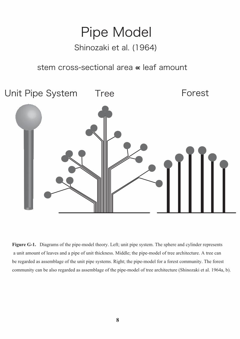
Pipe Model

Unit Pipe System Tree Forest

Shinozaki et al. (1964)

stem cross-sectional area ∝∝ leaf amount

Figure G-1. Diagrams of the pipe-model theory. Left; unit pipe system. The sphere and cylinder represents

a unit amount of leaves and a pipe of unit thickness. Middle; the pipe-model of tree architecture. A tree can

be regarded as assemblage of the unit pipe systems. Right; the pipe-model for a forest community. The forest

community can be also regarded as assemblage of the pipe-model of tree architecture (Shinozaki et al. 1964a, b).

8

Figure G-2. Sketches for branching rules by Leonardo da Vinci.

He mentioned that ‘the sum of cross-sectional areas of branches at any height equals to the cross-sectional area

of the trunk’ (Richter 1970). This also means that, in a branching point, the sum of branch cross-sectional areas

of daughter branches at immediately above the branching point equals to the branch cross-sectional area of the

mother branch at immediately below the branching point.

Sketches are from ‘The notebooks of Leonardo da Vinci’ (Richter 1970).

9

10

(Chapter 1)

Dependency of branch diameter growth in young Acer trees

on light availability and shoot elongation

Introduction

The cross-sectional area (or sapwood area) of a branch is proportional to the leaf mass

or leaf area of the branch. This relationship had been noted by Leonardo da Vinci as

long as 500 years ago (Richter 1970). On the basis of this proportional relationship,

Shinozaki et al. (1964a, b) proposed that a tree is an assemblage of pipes having the

same amount of leaves. This is called the pipe-model theory.

The pipe-model theory has been used in many studies that modeled tree growth

(Valentine 1985, Mäkelä 1986, 1997, 1999, 2002; Chiba et al. 1988; Chiba 1990, 1991,

Nikinmaa 1992, Chiba and Shinozaki 1994, Perttunen et al. 1996, 1998, Kershaw and

Maguire 2000, Koskela 2000) and water conduction (Waring et al. 1982, Ewers and

Zimmerman 1984a, b, Yamamoto and Kobayashi 1993). Several improvements to the

pipe model have been suggested from the viewpoints of biomechanics and water

conduction (Oohata and Shinozaki 1979, Chiba 1998, West et al. 1999, Berthier et al.

2001).

The ratio of leaf area (or leaf mass) to the sapwood area of the stem is, however,

not always constant. The ratio differs depending on site conditions as well as the

particular environment of a tree (Mäkelä et al. 1995, Mencuccini and Grace 1995,

Berninger and Nikinmaa 1997, Carey et al. 1998, Mäkelä and Vanninen 1998, Li et al.

2000). The ratio tends to decrease with the increase in tree height (McDowell et al.

2002). The ratio also tends to decrease when the sapwood area is measured at the lower

stem position (Mäkelä et al. 1995). These suggest that hydraulic conductance declines

with the increase in path length and/or sapwood senescence.

11

Photosynthates produced in leaves are translocated from these source leaves to

other sink organs along a gradient in sugar concentration. However, photosynthates

produced in a given branch are hardly translocated to its sibling branches, even when

there is the gradient in sugar concentration between branches. This feature is called

“branch autonomy” (Sprugel et al. 1991). The idea of branch autonomy has been used

in many studies of the mechanisms of construction of tree architecture (Takenaka 1994,

Perttunen et al. 1996, Day and Gould 1997) or of community structure (Takenaka 1994,

King et al. 1997). For example, Takenaka (1994) succeeded in mimicking the growth of

a stand of trees by assuming that each autonomous shoot produces its daughter shoots or

dies depending on the magnitude of its light interception.

However, it is misleading to treat all branches and shoots as being perfectly equal

and perfectly autonomous. Growth of a shoot depends on its local light environment and

its status among the neighboring daughter shoots within a branch (Takenaka 2000,

Sprugel 2002). Goulet et al. (2000) proposed the vigor index (VI) to express the relative

status of a branch. VI is calculated as follows. Consider a mother branch furcating

several daughter branches at a branching point. The VI of the thickest branch among

these daughter branches equals the VI of the mother branch. The VI of any other

daughter branch is expressed as a product of the VI of the mother branch and the ratio

of the cross-sectional area of this daughter branch to that of the thickest daughter branch.

VI, thus, represents the relative size of each daughter branch. The calculation starts with

the basal trunk and is repeated at every branching point. The VI values for the branch

segments of the main axis of the tree are set to 1. Accordingly, VI decreases as

branching order increases. When branch sizes are similar, the branches in the upper part

of the crown generally have greater VI than those in the lower part of the crown (Goulet

et al. 2000, Nikinmaa et al. 2003). In young trees of sugar maple (Acer saccharum

Marsh.) and yellow birch (Betula alleghaniensis Britt.) (Goulet et al. 2000) and in Scots

pine (Pinus sylvestris L. (P. silvestris L.)) (Nikinmaa et al. 2003), the growth of shoots

depended on both their light environment and VI.

The construction and maintenance of the branches, trunk, and root system rely on

the photosynthates produced by young shoots. Diameter growth of the branches

downstream of the distal shoots would not be solely determined by the local conditions

such as light interception or amount of leaves at the branch. In photosynthetically active

12

shoots, the ratio of photosynthates exported downwards to those used within the shoot

would also vary from shoot to shoot. For these reasons, the allocation pattern of

photosynthates should be more heterogeneous than that predicted by the pipe-model

theory. To understand how an entire tree is constructed, it is thus important to clarify the

allocation pattern of photosynthates. Although Valentine (1985), Mäkelä (1986, 1999,

2002), and Perttunen et al. (1996, 1998) developed plausible tree growth models that

incorporated rules for the allocation of photosynthates, the rules per se have not been

clarified. One of the potential mechanisms might be the abundance of long or leader

branches that would show high levels of auxin synthesis. Auxin synthesized in young

leaves and at active apices is directionally transported from the apices in the basal

direction, and activates shoot elongation and the cambial function (Mohr and Schopfer

1995). Therefore, branches having long shoots or leaders would also show vigorous

diameter growth. Such heterogeneous nature can be incorporated into the pipe-model

paradigm. In their pioneering study, Morataya et al. (1999) found that leaf mass was

correlated with area and volume growth of the sapwood in Tectona grandis L.f. and

Gmelina arborea Roxb..

Photosynthesis and transpiration are the most important functions in studying tree

growth and depend on irradiance. In-situ measurement of their rates for each shoot of

the tree is not practical, but light interception can be accurately estimated for each shoot.

An instantaneous photosynthetic light-response curve (the rate of photosynthesis plotted

against irradiance) shows obvious light saturation. Daily photosynthesis plotted against

daily photon flux density gives a much linearer curve (Terashima and Takenaka 1986).

Moreover, leaves in a canopy can acclimate to their respective light environments

(Björkman 1981). Therefore, the light interception by a shoot would be a reasonable

index of the photosynthesis by a shoot for a long time period such as weeks or months

(Campbell and Norman 1998).

In the present study, I used two maple species, Acer mono Maxim. var.

marmoratum (Nichols) Hara f. dissectum (Wesmael) Rehder and Acer rufinerve (Sieb.

& Zucc.), whose leaves have been shown to readily acclimate to their light

environments (Hanba et al. 2002). I measured light interception by each current-year

shoot for the index of photosynthetic production and transpiration. Then, I examined

the:

13

(1) relationships between current-year growth of cross-sectional area of a branch and

various leaf attributes, including leaf mass, leaf area, and light interception,

(2) relationships between current-year growth of cross-sectional area of a branch and

the current-year increase in the leaves,

(3) patterns of allocation of carbon from shoot tips to the base of the trunk, and

(4) dependency of diameter growth of a branch on light intensity and the attributes of

shoot growth activity (average length of the current-year shoots and VI).

On the basis of the results, I discuss mechanisms of the diameter growth of the

branches and trunks.

Materials and methods

Study sites and species

The study was conducted in two deciduous, broad-leaved forests. One was the Ogawa

Forest Reserve (36°56′N, 140°35′E, 600 m above sea level). The annual mean

temperature is 9.0°C and the mean annual precipitation is 1800 mm. The other was the

Ashu Experimental Forest of Kyoto University (35°20′N, 135°45′E, 700 m above sea

level). The annual mean temperature is 12.3°C and the mean annual precipitation is

2400 mm.

Three Acer mono Maxim. var. marmoratum (Nichols) Hara f. dissectum (Wesmael)

Rehder trees of 1–2 m (1.45 ± 0.37 m, mean ± S.D.) in height in the Ogawa Forest and

six A. rufinerve (Sieb. & Zucc.) trees of 0.5–3 m (1.56 ± 0.86 m) in the Ashu

Experimental Forest were selected from various light environments. The trees ranged

from 3 to 15 years old and had not suffered from any injuries. The total number of

current-year shoots examined was about 150 for A. mono and 350 for A. rufinerve. I

used all these current-year shoots for analyses. Data were collected in 1997 for A. mono

and in 1998 for A. rufinerve.

A. rufinerve is pioneer and A. mono is sub-climax species. Both are deciduous,

broad-leaved, semi-shade-tolerant trees that often reach the forest canopy at maturity.

14

Their phyllotaxis is decussate and their branching pattern is monopodial (Sakai 1990).

In both species, leaf expansion as well as the secondary growth of stems started in early

May. The secondary growth finished between mid-August and mid-September in A.

mono and in early September in A. rufinerve (Komiyama et al. 1987, 1989). Both

species have diffuse-porous wood.

Measurement of the light environment

I assessed the light environments of all 500 current-year shoots in the field before leaf

shedding. The relative irradiance of a given current-year shoot (RIS), which is the ratio

of irradiance measured just above the shoot to that measured at an open site, was

obtained under diffuse light conditions, and RIS was used as an index of the light

environment of the shoot.

For A. mono, RIS was estimated from hemispherical photographs (Pearcy 1989)

analyzed using the software, HEMIPHOT (ter Steege 1994). I took hemispherical

photographs just above each current-year shoot with a film camera (Nikomat, Nikon,

Tokyo, Japan) fitted with a fish-eye lens (Fisheye, Nikon) on cloudy days in October

1997. The lens was kept horizontally when the photographs were taken. For

current-year shoots that were too close to each other to allow us to take separate

photographs, I took one photograph just above their center. From the hemispherical

photographs, I calculated an indirect diffuse site factor (ISF) with HEMIPHOT. ISF was

calculated on the assumption that the sky was uniformly overcast. I used ISF above each

current-year shoot (ISFS) as an index of RIS. The highest value of RIS in each of the

three A. mono trees was 0.052, 0.142, and 0.189, respectively.

For A. rufinerve, I measured photosynthetically active photon flux density (PPFD;

µmol photons m–2 s–1) with quantum sensors (LI-190SB, LI-COR, Lincoln, NE, USA)

in addition to the analysis with hemispherical photographs. These measurements were

carried out on cloudy days in September 1998. I used two sensors. One was connected

to a datalogger (Thermodac-E, Eto Denki Co., Ltd, Tokyo, Japan) and placed

horizontally at a relatively open site on a forest road. The data were recorded every 5 s.

The second sensor was kept horizontally just above the current-year shoot, and PPFD

incident on the shoot (PPFDS) was measured. The measurements with the two sensors

15

were carried out at the same time, and the ratio of PPFD above the shoot to that at the

open site (RPPFDS) was calculated (Messier and Puttonen 1995, Parent and Messier

1996). I also took a hemispherical photograph at the same open site where the first

quantum sensor was placed, and calculated the ISF of the open site (ISFO) with

HEMIPHOT. I used ISFO to correct RIS (= ISFS = RPPFDS × ISFO) for each

current-year shoot. The highest value of RIS in each of the six A. rufinerve trees was

0.855, 0.722, 0.570, 0.299, 0.056, and 0.045, respectively.

For RPPFD < 0.7, instantaneous RPPFD under an overcast sky is strongly

correlated with the mean daily RPPFD under a clear sky (r2 = 0.872) as well as with the

mean daily RPPFD under a overcast sky (r2 = 0.969) (Messier and Puttonen 1995,

Parent and Messier 1996). Thus, I did not take into account the effects of direct light.

Measurement of leaf attributes

I collected all leaves and measured the total leaf area on each current-year shoot (AfS).

For A. mono, I measured the leaf area with a leaf area meter (AAM-7, Hayashi Denko

Co., Ltd, Tokyo, Japan). For A. rufinerve, I photocopied the leaves from each

current-year shoot, digitized the images with a scanner (JX-250, Sharp, Osaka, Japan),

and measured their areas with the NIH-Image v. 1.55 software (US National Institutes

of Health). The product of AfS and RIS was regarded as the light interception by the

current-year shoot (IfS = AfS × RIS). The leaves were then dried at 80°C for 2 to 3 days

and weighed to obtain the total leaf mass of the current-year shoot (WfS). These leaf

attributes (WfS, AfS, and IfS) are collectively referred to as FS.

I estimated three leaf attributes for each branch: Wf, Af, and If (F). Each of the trees

was notionally separated at every branching point and regarded as a fractal-like

structure consisting of branch modules. A large branch module included many small

branch modules, and the largest branch module in a tree was the tree itself. The

weighted relative irradiance of a branch (RI) was calculated as If/Af.

I also counted the number of the current-year leaves in the branch (Nf) and the

number of the leaf scars on the one-year-old branch in the whole branch. The latter

equals to the previous-year leaf number in the branch (Nf-1). I then estimated the

current-year increment of the leaf number (∆Nf = Nf – Nf-1). Nf, ∆Nf, F and RI were

16

estimated for all branch modules in all trees.

Measurement of stem attributes

After collecting the leaves, I cut down the trees and brought them back to the laboratory.

The lengths of all current-year shoots and of the branch segments between neighboring

branching points were measured with a measuring tape. For very short samples, I used

digital calipers (500-301, Mitutoyo Corporation, Kawasaki, Japan).

The greatest diameter (D) perpendicular to the length was measured at the base of

each current-year shoot and at the middle point of each branch segment using the digital

calipers. The diameters of the trunks at the bases of the crown and of the trunk were

also measured. Using these diameters, I calculated the cross-sectional areas of the

current-year shoots (AS) and of the branch segments and trunk (A): A or AS = πD2/4. For

A of the branch, A of the most basal branch segment within the branch or of the trunk

just below the crown was used. Areas were estimated for all the branches of all the

sample trees. All the branch and trunk cross-sections were wet and had a similar whitish

color. Hence, there was no heartwood in the samples.

The current-year growth in cross-sectional area was estimated for each of the

branches. To do so, I cut the branch segments or trunks at the position where the

diameter was measured. At the greatest diameter of the section, I measured the diameter

of the annual ring of the current year, excluding the bark and phloem, and that of the

annual ring of the previous year. The annual rings were identified by using a loupe. The

difference between the areas enclosed by the current-year and the previous-year annual

rings was regarded as the current-year's growth in cross-sectional area of the branch

segment or trunk (∆A). For each branch, ∆A of the most basal branch segment within

the branch or ∆A of the trunk just below the crown base was used. In some branch

segments with very dense annual rings, the current-year thickenings were not estimated.

Status of each branch

The length of each current-year shoot was measured, and the mean length of the

current-year shoot (

!

LS) was obtained for each branch. The vigor index (VI) was

17

calculated according to Goulet et al. (2000).

Statistics

For all statistical analyses, I used StatView J-4.5 software (Abacus Concepts, Inc.,

Berkeley, CA, USA). I used a linear regression analysis for the relationships between

leaf attributes and stem attributes. I also used multiple regression and partial correlation

to test the dependency of the diameter growth of a branch on the light intensity (RI),

average length of current-year shoots ( LS), and vigor index (VI) of the branch.

Results

Cross-sectional branch area and area growth vs. leaf attributes

I analyzed the relationships between cross-sectional area (A) and leaf attributes (F) for

all branch modules within the crowns (Figure 1-1). As leaf mass (Wf) or leaf area (Af)

increased, A increased proportionally in both species (r2 = 0.90–0.95). The coefficients

of determination in the relationships between light interception (If) and A (r2 = 0.78 and

0.87) were smaller than those for Wf and Af. The slopes of the relationships between A

and If varied depending on the relative irradiances experienced by the trees. Trees

growing in environments with high relative irradiance had smaller slopes for these

relationships than those in low relative irradiance (The regression lines for respective

irradiances are not shown).

When the current-year area growth of a branch (∆A) was plotted against F, the data

points were more scattered than those in Figure 1 (r2 = 0.45–0.87) (Figure 1-2). It is,

however, noteworthy that, in contrast to the results of the relationships between A and F

(Figure 1-1), the coefficients of determination were clearly greater for If (r2 = 0.75 and

0.87) than those for Wf (r2 = 0.66 and 0.70) and Af (r2 = 0.45 and 0.67).

18

Cross-sectional area growth of branch vs. leaf increment

If A is always proportional to F and there is no heartwood formation, current-year

growth of cross-sectional area of the branch should be proportional to the annual

increments in the leaf attributes (Valentine 1985, Mäkelä 1986). In Scots pine,

Nikinmaa (1992) observed that difference in cross-sectional area growth of the trunks

between just basipetal and acropetal of a given whorl was correlated with growth of the

needle mass for the whorl. This observation implies that the amount of newly formed

wood is correlated with the amount of new leaves.

We examined the relationships between the current-year cross-sectional area

growth of a branch (∆A) and the annual increment of the leaf number (∆Nf) (Figure 1-3).

In A. rufinerve, proportionality in the relationships between ∆A and ∆Nf (r2 = 0.86) was

stronger than that between ∆A and the current-year leaf number (Nf) (r2 = 0.54). In A.

mono, the proportionality was slightly stronger in the relationships between ∆A and ∆Nf

(r2 = 0.67) than that between ∆A and Nf (r2 = 0.61).

Patterns of carbon allocation from branch tip to trunk base

The pipe model assumes that the cross-sectional area of a branch is equal to the

cumulative cross-sectional area of its daughter branches (Shinozaki et al. 1964a, Richter

1970, Nikinmaa 1992, Yamamoto and Kobayashi 1993). Thus, I analyzed the

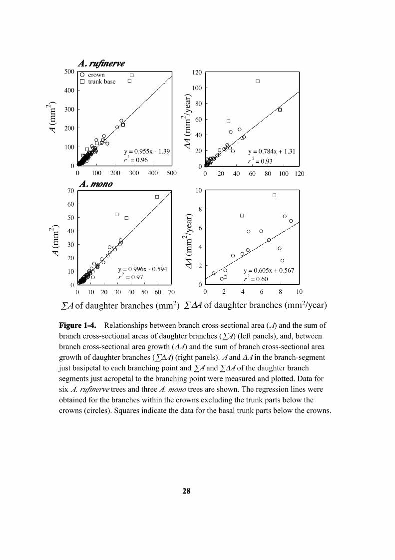
relationships between A and ∑A and between ∆A and ∑∆A for every branching point.

For each branching point, A or ∆A of a branch segment at just basipetal to the branching

point and ∑A or ∑∆A of all the branch segments at just acropetal to the branching point

were measured and plotted (Figure 1-4). For the branching points within the crowns, A

was almost identical to ∑A of the daughter branches in both species (slope = 0.96 and

1.0, r2 = 0.96 and 0.97). However, A values obtained at the trunk base tended to be

larger than ∑A. In contrast, ∆A for the branching points within the crowns was smaller

than ∑∆A for the daughter branches in most cases (slope = 0.78 and 0.61), although the

coefficient of determination for A. mono was not very large (r2 = 0.93 in A. rufinerve

and 0.60 in A. mono). However, again, ∆A values for basal trunks were larger than ∑∆A

for the daughter branches.

19

Dependency of branch diameter growth on light intensity and shoot growth activity

I analyzed the dependency of the branch diameter growth on its light environment and

on the relative status of the branch. Relative irradiance (RI) was used as an index of the

light environment of the branch. To indicate the relative status of a branch, we used the

average length of its current-year shoots ( LS) in the branch and the vigor index (VI) of

the branch. With partial correlation and multiple regression analyses, we tested the

effects of these parameters on the branch growth in cross-sectional area per unit of leaf

area (∆A/Af).

∆A/Af was correlated with LS in both species (Table 1-1). Although ∆A/Af was

correlated with RI in A. rufinerve, it was not significant in A. mono. VI had not effect on

∆A/Af in both species. There were not significant or not strong partial correlations

among LS, RI, and VI (Table 1-1).

The multiple regression model used here is:

∆A/Af = b0 + b1(RI) + b2( LS) + b3(VI),

where b0 is a constant and b1, b2, and b3 are partial regression coefficients. The

coefficient of determination (R2) for A. rufinerve was larger than that for A. mono (Table

1-2). LS was a significant determinant for both species. RI was significant only for A.

rufinerve. VI was not significant in either species.

Discussion

Two assumptions of the pipe model are that there is a proportional relationship between

branch cross-sectional area (or sapwood area) and leaf mass (or area), and that the sum

of branch area just acropetal to a branching point equals the branch area just basipatal to

the branching point. The results of this study indicate that these assumptions are

generally valid (Figure 1-1 and left panels of Figure 1-4). Although it was reported for

Scots pine (Nikinmaa 1992) and Cryptomeria japonica (L.f.) D. Don (Yamamoto and

Kobayashi 1993) that the cross-sectional area of the trunk at the crown base was smaller

than the sum of branch cross-sectional area, these trees were large (diameter > 10 cm)

20

and the stems included heartwood.

In the presented investigation, these two assumptions were not valid for the

current-year growth in cross-sectional area. For the branches within the crowns,

∆A/∑∆A was markedly smaller than 1, and ∆A/F gradually decreased with increment of

branch size (Figure 1-2 and the right panels of Figure 1-4). These trends indicate that

the diameter growth per unit of leaf area decreased toward the base. In other words, the

carbon allocation decreased toward the basal direction within the crown.

The proportion of the current-year cross-sectional area growth to the cross-sectional

area (∆A/A) generally decreases with increasing branch size and age. This fact and the

constant A/∑A and A/F ratios explain that the slopes in the right panels of Figure 1-4 are

smaller than 1. However, for the basal parts of the trunks, A was larger than ∑A (left

panels of Figure 1-4). Shinozaki et al. (1964a) explained that swelling of the trunk base

is due to the accumulation of disused pipes (i.e., of heartwood). These pipes, according

to their explanation, had been connected to old branches that died back. However, ∆A

was larger than ∑∆A at the trunk base (right panels of Figure 1-4). This means that

material allocation increased toward the trunk base and that this also contributes to

swelling of the trunk base. Other researchers have suggested that when the stems

develop heartwood and the leaf turnover rate is faster than the rate of heartwood

formation, newly formed sapwood area per unit of new leaf area decreases (Kershaw

and Maguire 2000, Vanninen and Mäkelä 2000, Valentine 2001, Mäkelä 2002). This

potentially explains the decrease in ∆A/∑∆A with crown depth. However, in the present

samples, there was no heartwood. If the age of the sapwood is greater than the leaf age,

the leaves are connected to the older xylem as well as to the current-year xylem. It is

always the case in deciduous Acer species having sapwood of multiple ages. This would

at least partly explain the trend in the present study, in which ∆A/∑∆A was smaller than

1 within the crown. The swelling at the trunk base would also contribute to mechanical

support (Oohata and Shinozaki 1979) and to the increment of sapwood area per leaves

(Mäkelä et al. 1995). It is probable that the inner xylem at the trunk base may gradually

die back and have very low water conductivity.

The coefficients of determination between A and If were smaller than those for Wf

and Af (Figure 1-1). In the shaded parts, A/If was larger. It was reported that the sap

flow rate was higher in the outer xylem than in the inner xylem (Kozlowski and

21

Pallardy 1997, Domec and Gartner 2003). Sapwood of older stems in shaded site may

show steeper radial gradient of water conductivity than that in bright sites. In contrast, If

was a better determinant of ∆A than Wf or Af (Figure 1-2), indicating that light

interception is more important for branch diameter growth than is leaf area or leaf mass.

The strong relatioships between ∆A and If imply that the xylem produced in the current

year would be a major pathway for the sap flow in these maple species.

On the other hand, ∆A was strongly dependent on the leaf number increment (∆Nf)

in A. rufinerve (Figure 1-3). However, in A. mono, this relationship was not stronger

than that between ∆A and Nf, and the plot patterns were similar to each other. These

indicate that ∆Nf are proportional to Nf. This phenomenon would be found in two cases.

(1) Sample trees are very young and small and ∆Nf is a major portion of Nf. (2) Sample

trees are very old or located in the shaded sites. All shoots show little elongation, and

leaf increment is very small and constant. Then, sink strength is homogenous among the

branches within a tree. The case of A. mono trees was probably (1). The strong

relationship between ∆A and ∆Nf is consistent with the theoretical predictions

(Valentine 1985, Mäkelä 1986). The above findings raise two questions: Which factor is

important for stem diameter growth, light interception or leaf increment? What are the

physiological mechanisms?

The diameter growth of branch per leaf area (∆A/Af) depended on RI in A.

rufinerve, but not in A. mono (Tables 1-1 and 1-2). The reason for the poor dependency

in A. mono could be due to the much smaller variation in RI observed in the A. mono in

my study (RI = 0.007–0.189) than was observed in A. rufinerve (RI = 0.011–0.855).

Hanba et al. (2002) showed that leaf mass per area (LMA) and photosynthetic capacity

on a leaf-area basis increase with site irradiance in both of these Acer species. Thus, RI

probably affected photosynthetic production in A. mono as well as in A. rufinerve.

It is noteworthy that ∆A/Af depended on the average length of the current-year

shoots in the branch ( LS) for both species (Tables 1-1 and 1-2). This means that the

elongation rate of the whole branch was important for the diameter growth of the branch.

Elongation of the current-year shoot would promote an annual increment in leaf number

because long shoots generally have more leaves. Auxin, synthesized in active shoot

apices and young leaves, is transported basipetally from the tips and activates branch

elongation and cambial growth (Mohr and Schopfer 1995). It is highly probable that the

22

branch diameter growth was enhanced by auxin synthesized by many long shoots or

leaders. On the other hand, many short shoots receiving strong light would be net

producers (i.e. sources rather than sinks) of photosynthates and probably contributed to

the growth of the trunk parts, in particular swelling of the trunk base and growth of the

root system.

Goulet et al. (2000) and Nikinmaa et al. (2003) showed that shoot elongation

depends on light intensity and on the vigor index (VI) of the shoot. In my results, the

partial correlations among LS, RI and VI of the branch were not significant or not strong

(Table 1-1). Moreover, VI of the branch was not a good determinant of ΔA of the

branch. This was probably because the elongation and VI of respective shoots showed

large variation even within a branch. Moreover, respective Ls within branches with

similar RI or VI differed considerably (data not shown). Some individual branches

contained both long and short shoots, and both a leader and lateral daughter branches.

From these considerations, the major factor responsible for the leaf increment

(∆Nf) would be shoot elongation ( LS). Thus, the diameter growth of the branch (∆A)

within the crown would be determined by the balance between supply of photosynthates,

which depends on light conditions (RI), and the demand created by the high cambial

activity that was enhanced by vigorous shoot elongation ( LS or ∆Nf).

23

Table 1-1. Partial correlation coefficients for the relationships between cross-sectional

area growth per unit of leaf area (∆A/Af), relative irradiance (RI), average current-year

shoot length ( LS), and vigor index (VI) of branches of A. rufinerve and A. mono. P <

0.05 was considered significant. n.s. = not significant.

Partial correlation coefficients

A. rufinerve (n = 193) A. mono (n = 77)

Relationship r p r p

∆A/Af vs. RI 0.575 <0.0001 0.194 0.095 n.s.

∆A/Af vs. LS 0.482 <0.0001 0.601 <0.0001

∆A/Af vs. VI 0.031 0.670 n.s. -0.137 0.241 n.s.

RI vs. LS 0.185 0.010 0.151 0.196 n.s.

RI vs. VI 0.050 0.492 n.s. 0.229 0.048

LS vs. VI 0.123 0.090 n.s. 0.149 0.202 n.s.

24

Table 1-2. Partial and standardized regression coefficients for the multiple regression

analysis of cross-sectional area growth per leaf area (∆A/Af) as a function of relative

irradiance (RI), average shoot length ( LS), and vigor index (VI) of branches of A.

rufinerve and A. mono. P < 0.05 was considered significant. n.s. = not significant.

Explanatory

variables

Partial regression

coefficients

Standardized partial regression

coefficients P

A. rufinerve (n = 193, R2 = 0.710, P < 0.0001)

RI 1.766 × 10–4 0.511 <0.0001

LS (mm) 3.332 × 10–7 0.404 <0.0001

VI 3.040 × 10–6 0.017 0.673 n.s.

Intercept 1.236 × 10–5 1.236 × 10–5 0.017

A. mono (n = 77, R2 = 0.445, P < 0.0001)

RI 1.392 × 10–4 0.162 0.095 n.s.

LS (mm) 5.835 × 10–7 0.605 <0.0001

VI -7.668 × 10–6 -0.107 0.241 n.s.

Intercept 2.420 × 10–5 2.420 × 10–5 0.0004

Note: The regression model is ∆A/Af = b0 + b1(RI) + b2( LS) + b3(VI), where b0 are

constants, bn are partial regression coefficients.

GG

G

GGGGGGGGGGG

GGGGG

G

G

GGGG

G

GGGGGGGGGGGG

G

GGGGGGGGGGGGGGGGGGGGGGGGGGGGGGGGGGGGGGGGGGGGGGGGGGGGG

GGG

GG

G

G

G

GG

G

GGG

G

G

GG

G

GG

G

GG

G

GG

G

GGGGGGGG

G

GGGG

G

GGGGGGGGGGGGGG

G

G

G

G

G

GGGGGGGGGGGGG

G

G

GGG

G

G

GG

GGGGGGGGG

G

GGGGGGGGGGGGGGGGGGGGGGGGGGGGGGGGGGGGGGGGGGGGGG

GGGG

G

GG

GGG

G

G

G

GGGG

G

GGG

G

GGGG

GGG

G

G

G

G

GGGG

GG

G

G

G

G

G

G

G

G

G

G

EEEEEEEEEEEEEEEEEEEEEEEEEEEEEEEEEEEEEEEEEEEEEEEEEEEEEEEEEEEEEEEEEEEEEEEEEEEEEEEEEEEEEEEEEEEEEEEEEEEEE

EE

EE

E

E

E

EE

E

E

E

EE

E

E

E

EEEEEEE

E

E

EEEEEEEEEEE

EE

EE

E

EEE

E

EEEEE

EE

E

EE

E

EE

E

EE

E

E

E

E

E

EEEEE

E

E

E

E

EE

E

EEEEEE

E

EEEE

E

EE

E

EEEEEEEEEEE

E

EEEEEEEEEE

E

E

E

EEEEEEEEE

E

E

E

E

EEEEEEEEEEE

E

E

E

CCCCCCCCCCCCCCCCCCCCCCCCCCCCCCCCCCCCCCCCCCCCCCCCCCCC

C

C

C

C

CCCCC

C

CCCCCCCCCCC

C

CCCCCCCCCCCC

C

C

CCCCCCCCCCCCCCCCCCCCCCCCCCC

CCCCCCCCCCC

C

C

0

50

100

150

200

250

0 10 20 30 40 50 60 70

GG

G

GGGGGGGGGGG

GGGGG

G

G

GGGG

G

GGGGGGGGGGGG

G

GGGGGGGGGGGGGGGGGGGGGGGGGGGGGGGGGGGGGGGGGGGGGGGGGGGGG

GGG

GG

G

G

G

GG

G

GGG

G

G

GG

G

GG

G

GG

G

GG

G

GGGGGGGG

G

GGGG

G

GGGGGGGGGGGGGG

G

G

G

G

G

GGGGGGGGGGGGG

G

G

GGG

G

G

GG

GGGGGGGGG

G

GGGGGGGGGGGGGGGGGGGGGGGGGGGGGGGGGGGGGGGGGGGGGG

GGGG

G

GG

GGG

G

G

G

GGGG

G

GGG

G

GGGGGGG

G

G

G

G

GGGG

GG

G

G

G

G

G

G

G

G

G

G

EEEEEEEEEEEEEEEEEEEEEEEEEEEEEEEEEEEEEEEEEEEEEEEEEEEEEEEEEEEEEEEEEEEEEEEEEEEEEEEEEEEEEEEEEEEEEEEEEEEEEEEEE

E

E

E

EE

E

E

E

EE

E

E

E

EEEEEEE

E

E

EEEEEEEEEEEEE

EE

E

EEE

E

EEEEEEE

E

EE

E

EE

E

EE

E

E

E

E

E

EEEEEE

E

E

E

EE

E

EEEEEE

E

EEEE

E

EE

E

EEEEEEEEEEE

E

EEEEEEEEEE

E

E

E

EEEEEEEEE

E

E

E

E

EEEEEEEEEEE

E

E

E

CCCCCCCCCCCCCCCCCCCCCCCCCCCCCCCCCCCCCCCCCCCCCCCCCCCC

C

C

C

C

CCC

C

CCCCCCCCCCC

C

CCCCCCCCCCCC

C

C

CCCCCCCCCCCCCCCCCCCCCCCCCCC

CCCCCCCCCCC

C

C

0 0.1 0.2 0.3 0.4

E

EEEEEEEEEEEE

EEEEEEEEEEEEEEEEEEEEEEEE

EEE

EE

E

E

E

EEEE

E

E

E

EE

E

EEEE

EEE

E

EE

E

EE

E

E

EE

E

E

E

EEEEEEEEEEEEEEEEEEEEEE

E

EEEEEEEEEEEEEEEEEEEEEEEEEEEEEEEEEEEEEEEEE

E

E

EEE

E

E

E

EE

E

EE

E

EEE

E

EE

EE

E

E

E

EEEE

E

EEEEE

E

EEEEE

E

E

EE

EE

E

E

E

E

E

E

EEEEE

EE

EE

E

E

CCCCCCCCCCCCCCCCCCCCCCCCCCCCCC

C

C

CCCC

C

C

C

CCCCC

C

C

C

C

C

0 0.01 0.02 0.03

E

EEEEEEEEEEEE

EEEEEEEEEEEEEEEEEEEEEEEE

EEE

EE

E

E

E

EEEE

E

E

E

EE

E

EEEE

EEE

E

EE

E

EE

E

E

EE

E

E

E

EEEEEEEEEEEEEEEEEEEEEE

E

EEEEEEEEEEEEEEEEEEEEEEEEEEEEEEEEEEEEEEEEE

E

E

EEE

E

E

E

EE

E

EE

E

EEE

E

EE

EE

E

E

E

EEEE

E

EEEEEEEEEE

E

E

EE

EE

E

E

E

E

E

E

EEEEE

EE

EE

E

E

CCCCCCCCCCCCCCCCCCCCCCCCCCCCCC

C

C

CCCC

C

C

C

CCCCC

C

C

C

C

C0

10

20

30

40

0 2 4 6 8 10 12

GG

G

GGGGGGGGGGG

GGGGG

G

G

GGGG

G

GGGGGGGGGGGG

G

GGGGGGGGGGGGGGGGGGGGGGGGGGGGGGGGGGGGGGGGGGGGGGGGGGGGG

GGG

GG

G

G

G

GG

G

GGG

G

G

GG

G

GG

G

GG

G

GG

G

GGGGGGGG

G

GGGG

G

GGGGGGGGGGGGGG

G

G

G

G

G

GGGGGGGGGGGGG

G

G

GGG

G

G

GG

GGGGGGGGG

G

GGGGGGGGGGGGGGGGGGGGGGGGGGGGGGGGGGGGGGGGGGGGGG

GGGG

G

GG

GGG

G

G

G

GGGG

G

GGG

G

GGGG

GGG

G

G

G

G

GGGG

GG

G

G

G

G

G

G

G

G

G

G

EEEEEEEEEEEEEEEEEEEEEEEEEEEEEEEEEEEEEEEEEEEEEEEEEEEEEEEEEEEEEEEEEEEEEEEEEEEEEEEEEEEEEEEEEEEEEEEEEEEEE

EE

EE

E

E

E

EE

E

E

E

EE

E

E

E

EEEEE

EE

E

E

EEEEEEE

EEEE

EE

EE

E

EEE

E

EEE

EE

EE

E

EE

E

EE

E

EE

E

E

E

E

E

EEE

EE

E

E

E

E

EE

E

EEEEEE

E

EEEE

E

EE

E

EEEEEEEEEEE

E

EEEEEEEEE

E

E

E

E

EEEEEEEEE

E

E

E

E

EEEEEEEEEEE

E

E

E

CCCCCCCCCCCCCCCCCCCCCCCCCCCCCCCCCCCCCCCCCCCCCCCCCCCC

C

C

C

C

CCC

C

CCCCCCCCCCC

C

CCCCCCC

CCCCC

C

C

CCCCCCCCCCCCCCCCCCCCCCCCCCC

CCCCCCCCCCC

C

C

0 0.2 0.4 0.6 0.8 1 1.2

E

EEEEEEEEEEEE

EEE

EEEEEEEEEEEEEEEEEEEEE

EEE

EE

E

E

E

EEEE

E

E

E

EE

E

EEEE

EEE

E

EE

E

EE

E

E

EE

E

E

E

EEEEEEEEEEEEEEEEEEEEEE

E

EEEEEEEEEEEEEEEEEEEEEEEEEEEEEEEEEEEEEEEEE

E

E

EEE

E

E

E

EE

E

EE

E

EEE

E

EE

EE

E

E

E

EEEE

E

EEEEEEEEEE

E

E

EE

EE

E

E

E

E

E

E

EEEEE

EE

EE

E

E

CCCCCCCCCCCCCCCCCCCCCCCCCCCCCC

C

C

CCC

C

C

C

C

CCCCC

C

C

C

C

C

0 0.1 0.2 0.3

A. rufinerve

A. mono

A (m

m2 )

Wf (g) Af (m2) If (m2)

y = 3.53x + 3.19r 2 = 0.94

y = 202x + 2.83r 2 = 0.95

y = 3.09x + 0.928 y = 121x + 0.530r 2 = 0.90 r 2 = 0.95

r 2 = 0.78

r 2 = 0.87

y = 641x + 5.62

y = 1300x + 0.960

G 20-40%E 5-20%C < 5%

A (m

m2 )

Figure 1-1. Relationships between branch cross-sectional area (A) and cumulative leaf parametersfor a branch (Wf, Af, and If) within the crown. Data for six A. rufinerve trees and three A. mono treesare shown. Symbols denote the relative irradiance levels for the trees. Squares, circles, and trianglesdenote relative irradiance of 20%-40%, 5%-20%, and <5%, respectively. The regression lines wereobtained without the data points for the trunk bases.

25

GGGGGGGGG

G

GGG

GGG

GGGGG

G

G

G

G

GG

GG

G

GGGGGGGG

GGGG

G

GG

GGG

GG

GGGGGG

G

GGGGG

GGG

G

GGGG

G

G

GGGG

G

EEEEE

E

EEE

E

EEEEE

E

EEEEEEEEE

E

EEEEEEE

E

E

EEEEEEE

EE

EEE

EE

E

EEE

E

E

EEEEE

E

EEEEEEE

E

CCCCCCCCCCCC CCCCCCCCCCC

CCCCCC

C

CCCCCCCCCCCCC0

20

40

60

80

0 10 20 30 40 50 60 70

EE

E

E

E

EE

EE

E

E

E

EE

E

EE

E

E

E

E

EEE

EE

EE

E

E

EE

E

E

EE

E

E

E

EE

EE

EE

E

E

E

E

E

E

EEEEE

EEECC

C

C

CC

CCCCC C

C

C

0

2

4

6

8

0 2 4 6 8 10 12

GGGGGGGGG

G

GGG

GGG

GGGGG

G

G

G

G

GG

GG

G

GGGGGGGG

GGGG

G

GG

GGG

GG

GGGGGG

G

GGGGG

GGG

G

GGGG

G

G

GGGG

G

EEEEE

E

EEE

E

EEEEE

E

EEEEEEEEE

E

EEEEEEE

E

E

EEEEEEE

EE

EEE

EE

E

EEE

E

E

EEEEE

E

EEEEEEE

E

CCCCCCCCCCCC CCCCCCCCCCC

CCCCCC

C

CCCCCCCCCCCCC

0 0.2 0.4 0.6 0.8 1 1.2

EE

E

E

E

EE

EE

E

E

E

EE

E

EE

E

E

E

E

EEE

EE

EE

E

E

EE

E

E

EE

E

E

E

EE

EE

EE

E

E

E

E

E

E

EEEEE

EEECC

C

C

CC

CCCCC C

C

C

0 0.1 0.2 0.3

GGGGGGGGG

G

GGG

GGG

GGGGG

G

G

G

G

GG

GG

G

GGGGGGGG

GGGG

G

GG

GGG

GG

GGGGGG

G

GGGGG

GGG

G

GGGG

G

G

GGGG

G

EEEEE

E

EEE

E

EEEEE

E

EEEEEEEEE

E

EEEEEEE

E

E

EEEEEEE

EE

EEE

EE

E

EEE

E

E

EEEEE

E

EEEEEEE

E

CCCCCCCCCCCCCCCCCCCCCCCCCCCCCC

CCCCCCCCCCCC

0 0.1 0.2 0.3 0.4

G 20-40%E 5-20%C < 5%

EE

E

E

E

EE

EE

E

E

E

EE

E

EE

E

E

E

E

EEE

EE

EE

E

E

EE

E

E

EE

E

E

E

EE

EE

EE

E

E

E

E

E

E

EEEEE

EEE

C

CC

CCCCC C

C

C

C

0 0.01 0.02 0.03

∆A (m

m2 /y

ear)

Wf (g) Af (m2) If (m2)

A. rufinerve

A. mono

y = 1.00x + 1.36 y = 47.2x + 2.65 y = 220x + 1.89

y = 0.656x + 0.891 y = 25.3x + 0.734 y = 292x + 0.830

r 2 = 0.66 r 2 = 0.45 r 2 = 0.87

r 2 = 0.70 r 2 = 0.67 r 2 = 0.75

∆A (m

m2 /y

ear)

Figure 1-2. Relationships between current-year growth of branch cross-sectional area (∆A) andcumulative leaf parameters for a branch (Wf, Af, and If) within the crown. For other information,see Figure 1-1.

26

GGGGGGGGG

G

GGG

GGG

GGGGG

G

G

G

G

GG

GG

G

GGGGGGGG

GGGG

G

GG

GGG

GG

GGGGGG

G

GGGGG

GGG

G

GGGG

G

G

GGGG

G

EEEEE

E

EEE

E

EEEEE

E

EEEEEEEEE

E

EEEEEEE

E

E

EEEEEEE

EE

EEE

EE

E

EEE

E

E

EEEEE

E

EEEEEEE

E

CCCCCCCCCCCC CCCCCCCCCCC

CCCCCC

C

CCCCCCCCCCCCC0

20

40

60

80

0 50 100 150 200 250

GGGGGGGGG

G

GGG

GGG

GGGGG

G

G

G

G

GG

GG

G

GGGGGGGG

GGGG

G

GG

GGG

GG

GGGGGG

G

GGGGG

GGG

G

GGGG

G

G

GGGG

G

EEEEE

E

EEE

E

EEEEE

E

EEEEEEEEE

E

EEEEEEE

E

E

EEEEEEE

EE

EEE

EE

E

EEE

E

E

EEEEE

E

EEEEEEE

E

CCCCCCCCCCCCCCCCCCCCCCCCCCCCCC

CCCCCCCCCCCCC

0 20 40 60 80 100 120 140

y = 0.262x + 1.91r 2 = 0.54

y = 0.709x + 1.58r 2 = 0.86

EE

E

E

E

EE

EE

E

E

E

EE

E

EE

E

E

E

E

EEE

EE

EE

E

E

EE

E

E

EE

E

E

E

EE

EE

EE

E

E

E

E

E

E

EEEEE

EEECC

C

C

CC

CCC

CC C

C

C

C

0

2

4

6

8

0 50 100 150 200

y = 0.0383x + 0.763r 2 = 0.61

EE

E

E

E

EE

EE

E

E

E

EE

E

EE

E

E

E

E

E EE

EE

EE

E

E

EE

E

E

EE

E

E

E

EE

EE

EE

E

E

E

E

E

E

EEEEE

EEECC

C

C

CC

CCC

CC C

C

C

C

0 20 40 60 80 100 120

y = 0.0568x + 0.731r 2 = 0.67

G 20-40%E 5-20%C < 5%

A. rufinerve

A. mono

∆Nf (/year)Nf

∆A (m

m2 /y

ear)

∆A (m

m2 /y

ear)

Figure 1-3. Relationships between current-year growth of branch cross-sectionalarea (∆A) and current-year leaf number (Nf), and, between ∆A and annual incrementin leaf number (∆Nf) within the crown. For other information, see Figure 1-1.

27

EEEEEEEEEE

E

EEEEE

E

E

EEE

E

EEE

E

EE

E

EEEEEEE

EEE

EEEEEEEE EEEE

E

EEEEEEE

EEEEEE

E

EEEEEEEEEEEEEE

E

EEEE

E

EEEEEEEEEE

EEEE

E

EEEEEEEEE

E

EEEEEEEE

E

EEEEEEEEEE

E

EE

EEEEEE

E

EEEEE

E

E

EEEEE

E

EEEEEE

EEEEEEEEE

EEE

E

EEEEEEE

E

EEEEE

E

EEEEEEEEEEEEGG

GG

G

G

G

G

G

0

100

200

300

400

500

0 100 200 300 400 500

EEEEE

EE

EEEE

EEE

EEE

E

EE

EEE

EEEE

E

EE

EE

E

EE

EEEE

E

E

E

EEE

E

EEEEEEEEEEEE

EEEEEEEEEEEEEE

EEEEE

E

E

E

G

G

G

0

10

20

30

40

50

60

70

0 10 20 30 40 50 60 70

E

E

EE

E

EE

EE

EEEE

E

EE

E

E

EE

EEE

EE

E

EEEEEEEEEEEEGG

G

G

G

G0

20

40

60

80

100

120

0 20 40 60 80 100 120

E

E

EE

E

E E

E

EE

EE

E

E

G

G

0

2

4

6

8

10

0 2 4 6 8 10

A. rufinerve

A. mono

∑A of daughter branches (mm2)

A (m

m2 )

∆A (m

m2 /y

ear)

∑∆A of daughter branches (mm2/year)

y = 0.955x - 1.39

y = 0.996x - 0.594

y = 0.784x + 1.31

y = 0.605x + 0.567

r 2 = 0.96

r 2 = 0.97

r 2 = 0.93

r 2 = 0.60

G trunk baseE crown

A (m

m2 )

∆A (m

m2 /y

ear)

Figure 1-4. Relationships between branch cross-sectional area (A) and the sum ofbranch cross-sectional areas of daughter branches (∑A) (left panels), and, betweenbranch cross-sectional area growth (∆A) and the sum of branch cross-sectional areagrowth of daughter branches (∑∆A) (right panels). A and ∆A in the branch-segmentjust basipetal to each branching point and ∑A and ∑∆A of the daughter branchsegments just acropetal to the branching point were measured and plotted. Data forsix A. rufinerve trees and three A. mono trees are shown. The regression lines wereobtained for the branches within the crowns excluding the trunk parts below thecrowns (circles). Squares indicate the data for the basal trunk parts below the crowns.

28

29

(Chapter 2)

Responses of the pipe-model relationships in Acer rufinerve

branches to artificial manipulations of light intensity, leaf

amount and shoot elongation: Perturbation and recovery Introduction

The pipe model theory of tree architecture indicates that a ratio of the total leaf area (or

leaf mass) cumulated for the branch to the basal cross-sectional area (or sapwood area)

of the branch is constant. The ratios of leaf area to sapwood area, however, differ

depending on growth habitats (Mäkelä et al. 1995, Mencuccini and Grace 1995,

Berninger and Nikinmaa 1997, Carey et al. 1998, Mäkelä and Vanninen 1998, Li et al.

2000). It was well documented that the ratios were lower in areas of arid climates

(Mencuccini and Grace 1995, Berninger and Nikinmaa 1997). The ratios decreased with

the increase in tree height (McDowell et al. 2002). The ratios were also low, when the

sapwood area was measured at the trunk base rather than the crown base (Mäkelä et al.

1995). The latter two tendencies suggest that the hydraulic conductance declines with

sapwood senescence and/or with the increase in the path length. In most of these studies,

the variation in the ratio was discussed from a viewpoint of plant water relation, and

roles of photosynthetic production and allocation of photosynthates in the pipe-model

relationship have not been taken into account.

Although the pipe model relationships are usually obtained between the total leaf

area (or leaf mass) cumulated for the branch and the basal cross-sectional area (or

sapwood area) of the branch, in A. rufinerve, a strong relationship between the leaf

number and the stem cross-sectional area of the branch was obtained (Figure 1-1 in

Chapter 1, see also Figure 2-2). This is because variations in leaf area or in leaf dry

mass among the leaves were not marked. The more important point is that this strong

relationship is realized because the increase in leaf number on a branch obviously is

30

correlated with growth in the branch size as already shown in Chapter 1. Then, the

mechanisms underlying the maintenance of the pipe-model architecture can be clarified

by analyzing the relationships between the leaf number and the stem cross-sectional

area.

It is widely observed that photosynthates produced by a given branch are

transported preferentially to downstream organs including the trunk and roots and rarely

transported to its neighbouring branches (Sprugel et al. 1991). However, this rule, called

‘branch autonomy’, does not suggest about an important point: how much

photosynthates are transported to in the downstream organs. These shares appear to

depend not only on its light environment but also on the status of the branch within the

tree. As for shoot elongation, the importance of the relative status among branches was

pointed out (Goulet et al. 2000, Takenaka 200, Sprugel 2002, Suzuki 2002, 2003,

Nikinmaa et al. 2003). Actually, the analyses described in Chapter 1 clearly showed that

the cross-sectional area growth of the branch depended on light interception and the

increment in leaf number. The leaf number increment also strongly correlated with the

branch growth rate such as elongation of the current-year shoots within the branch.

Hence, branch growth depends on both supply of photosynthates and demand for

photosynthates (Sone et al. 2005, Terashima et al. 2005, see also Terashima et al. 2002).

The supply is further analyzed into the leaf amount and light intensity. The increment of

the leaf amount and branch elongation should be important components of the demand

for photosynthates within the branch. Then, it is important to know how these

respective factors such as light intensity, leaf amount and shoot elongation interrelate to

maintain the affect the pipe-model relationship. In the experiments in Chapter 2, I

manipulated the light intensity, leaf amount and the shoot elongation of the branch and

analyzed responses of the branch attributes.

Materials and Methods Study site and plant materials

The study was conducted in a deciduous, broad-leaved forest (Ashu Experimental

Forest, Kyoto University, 35˚20’ stem N, 135˚45’ E, 700 m a.s.l.), where the mean

annual temperature is 12.3˚C and the mean annual precipitation is 2400 mm.

31

Five A. rufinerve (Sieb. et Zucc.) trees of 4 – 6 m in height were selected. In 2003,

the total number of current-year shoots and branches examined were about 2800 and

170, respectively. We used all the current-year shoots for analyses. Data were collected

in 2001, 2002 and in 2003.

A. rufinerve is a deciduous broad-leaved tree species that is pioneer and semi shade

tolerant. Mature trees of this species often reach the forest canopies. The phyllotaxis is

decussate and the branching pattern is monopodial (Sakai 1990). Leaf expansion and

the secondary growth of stems start in early May. The secondary growth ceases in early

September (Komiyama et al. 1987, 1989). This species has diffuse-porous wood.

Sample trees used in this study did not develop the heartwood yet.

Measurement of light environment of branches

The light environments of 170 branches were assessed in the field from July to

September in 2002 and 2003. Small pieces (15 * 25 mm) of the light sensitive film (Y-1

W, Pan, Taisei E&L, Tokyo) having the maximal sensitivity at 468 nm were attached on

the leaves and collected after exposure for several weeks. Light transmittance of the

film was measured before (T0) and after (T) the exposure.

Mean daily irradiance i (MJ m-2 day-1) was calculated as follws:

i = [-0.0101(100d/d0)2 – 0.5419(100d/d0) + 167.59]/day,

Where, d0 and d are:

d0 = -1.4154 log10T0 – 0.237

and

d = -1.4154 log10T – 0.237.

Measurement of leaf and stem attributes

Leaf and stem attributes were assessed in the field in November 2001, 2002 and 2003.

In November, diameter growth of the branches and trunks ceased and green leaves were

still on the branches in A. rufinerve. For each of the branches, the basal diameter (D)

was measured with calipers. Numbers of leaf (Nf), current-year shoots and of

32

current-year long shoots were counted. Length of long shoots (Ls) was measured with a

scale. The long shoots were defined as the shoots having four (two pairs) or more leaves.

The branch cross-sectional area (A) was calculated as A = D2/4. The current-year

growth of the branch cross-sectional area (∆A) was calculated as the difference between

the current-year A and previous-year A. The yearly increment of leaf number (∆Nf) was

similarly calculated as the difference between the current-year Nf and previous-year Nf.

The light interception of the branch (if) was calculated as if = Nf i.

Design of branch manipulations

One tree was used as a control tree (CT) and the other four trees were subject to

manipulations (manipulated trees, MTs). In each MT, the crown was divided into two

branch clusters. Branches in one cluster were untreated (control branches, CBs), and

those of the other cluster were subject to one of the manipulations (see below,

manipulated branches, MBs). The branches including most vigorous axes (i.e., leader

branches) were selected for MBs.

No manipulations were conducted in 2001. In May in 2002, MBs in MTs were

subject to either of the manipulations (Figure 2-1):

Shade: MBs within a MT were shaded by a frame (2.0 m width 2.5 m depth * 2.5 m

height) covered with black shade cloths. Mean daily irradiance (i) in the shade box was

about 15 % of the ambient i. By this manipulation, leaf numbers and leaf area in MBs

did not change, but the light interception of the MBs decreased to 15 % of original

levels.

Half cut: For all the leaves on MBs in a MT, acropetal halves of the laminas were

removed using scissors. By this manipulation, leaf numbers in MBs did not change, but

the total leaf area of the MBs decreased to the half.

Half pick: At each node in all the current-year shoots in MBs, one of the pair leaves

was removed. By this manipulation, both leaf number and the total leaf area decreased

to the half the original levels.

Long-shoot pick: From each of the long shoots on MBs in a MT, leaves and stems were

removed leaving the basal portions including the first two leaves (one pair). This

manipulation artificially changed all the current-year shoots to short shoots. By this

treatment, branch leaf number was reduced. Also, shoot elongation and the increase in

33

leaf area were suppressed.

In 2003, only the shade treatment was continued as was made in 2002 and the other

manipulations were not conducted.

Results

Control tree

The cross-sectional area of the trunk at the crown base and total leaf number for the tree

increased every year (Table 2-1). Very similar proportional relationships between the

branch cross-sectional area (A) and leaf number of the branch (Nf) were observed every

year (Figure 2-2 and 2-3). This indicates that the pipe-model relationship was

maintained for these three years and that yearly growth in branch cross-sectional area

(∆A) was almost proportional to yearly increment of leaf number of the branch (∆Nf) in

the CT (Figure 2-6, see also Figure 1-3 in Chapter 1, Sone et al. 2005). Ratios of the

branch cross-sectional area growth to leaf number (∆A/Nf) (Figure 2-4), light

interception (∆A/if) (Figure 2-5) and to cumulative length of long shoot (∆A/∑Ls)

(Figure 2-7) did not differ between 2002 and 2003.

Shade manipulation

A increased every year in CBs and MBs (Table 2-1). In 2002, Nf also increased in both

CBs and MBs, although the irradiance (i) for MBs decreased to 15%. In the second year

of the shade treatment, 2003, Nf decreased in MBs. The increase in Nf was also

suppressed in CBs, although CBs were not shaded.

The pipe-model relationship changed in response to the shade treatment (Figure 2-3).

A/Nf was reduced by the shading in 2002. The ratio, however, recovered in 2003,

although the shading continued in 2003 as well. The recovery was mainly attributed to

the decrease in Nf (Table 2-1). Interestingly, a similar tendency was observed in CBs

(Figure 2-3).

For either CBs or MBs, ∆A/Nf were similar between 2002 and 2003. ∆A/Nf were

somewhat lower in MBs than in CBs. On the other hand, ∆A/if was smaller in 2003 than

that in 2002 in both CBs and MBs. These indicate that MBs thickened despite of the

considerable decrease in photosynthetic production in 2002. In 2003, Nf and shoot

34

elongation were suppressed and ∆A followed its photosynthetic production. Thus,

∆A/∆Nf did not differ between CBs and MBs in 2002 (Figure 2-6). The difference in

∆A/∑Ls was not found in MBs between 2002 and 2003 (Figure 2-7). On the other hand,

in CBs, the ratio in 2002 declined although CBs were not shaded. In MBs, the

proportion of long shoots increased in 2002 and decreased in 2003. Inversely, in CBs,

the proportion decreased in 2002 and increased in 2003 (Table 2-1).

Half cut manipulation

In CBs and MBs, A increased every year (Table 2-1). Nf increased in 2002 and

decreased in 2003, although the leaves were not cut in 2003. The manipulation also

affected characteristics of CBs.

A/Nf of the MBs significantly declined in 2002 (Figure 2-3) probably because leaf

area and leaf mass decreased to half the original levels but the leaf number unchanged

by this manipulation. The ratio recovered in 2003 mainly due to the decrement in leaf

number (Table 2-1). Similar tendency was found in the CBs, although the leaves on

CBs were not cut (Figure 2-3).

In both branches, ∆A/Nf and ∆A/if were smaller in 2002 than in 2003 (Figure 2-4 and

2-5). These decreases in 2002 were expected because the leaf area and leaf mass were

reduced by the manipulation. Interestingly, these ratios also decreased in CBs. ∆A/∆Nf

in CBs and MBs of the half cut MT in 2002 were smaller than that in the CT. Within the

half cut MT, ∆A/∆Nf was significantly smaller in MBs than in CBs (Figure 2-6). This

indicates that effects of the manipulation were stronger in MBs than in CBs. The long

shoot proportion of the branch declined in both 2002 and 2003 in both CBs and MBs

(Table 2-1). From MBs, the long shoots disappeared in 2003. In CBs, ∆A/∑Ls in 2002

was considerably smaller than that in 2003 (Figure 2-7). This is because long shoot

number decreased substantially in 2003.

Half pick manipulation

In both CBs and MBs, A increased every year (Table 2-1). In MBs, Nf increased in 2002,

although the half of the leaves was removed. Nf markedly increased in 2003, because

new axillary buds developed at axils of the removed leaves. In contrast, Nf of CBs

decreased in 2003.

35

Although one half of the leaves were removed, the increase in A/Nf in 2002 was very

small (Figure 2-3). The ratio recovered in 2003 by the increase in Nf (Table 2-1). In CBs,

the increase in Nf was suppressed in 2002 and Nf decreased in 2003 (Table 2-1) and by

the decrease in Nf, A/Nf slightly increased in 2003 (Figure 2-3).

In both branches, ∆A/Nf and ∆A/if in 2002 were similar to those in 2003 (Figure 2-4

and 2-5). These indicate that the decreased photosynthetic production limited the branch

diameter growth. ∆A/∆Nf was greater in MBs than in CBs in 2002 (Figure 2-6). The

reason was light intensity was greater in MBs than in CBs as is evident by comparison

between Figure 2-4 and Figure 2-5. The long shoot proportion increased in 2002 and

decreased in 2003 in both branches (Table 2-1). Because one MB showed little

elongation but great thickening growth, the variance in ∆A/∑Ls for MBs was very large

in 2003 (Figure 2-7). When the data for this branch were excluded, there were only

small changes between the years in both MBs and CBs, and ∆A/∑Ls were smaller in

MBs than in CBs in both years.

Long-shoot pick manipulation

In both CBs and MBs, A increased in both years (Table 2-1). In MBs, Nf increased in

2002, even though long shoots were removed. Nf markedly increased in 2003, because

many long shoots developed in 2003. In contrast to the MBs, Nf decreased in 2003 and

the long shoot proportion decreased in both years in CBs. The long-shoot pick

manipulation of MBs in the previous year strongly affected development of long-shoots

and the leaf amount of CBs (Table 2-1).

Interestingly, when both the leaf amount (area plus number) and the shoot

elongation of the branch were suppressed by this manipulation, A/Nf did not change

(Figure 2-3). The ratio increased in 2003 because the increase in Nf was smaller

compared with stem growth (Table 2-1).

In both branches, ∆A/Nf and ∆A/if were almost similar between the two years

(Figure 2-4 and 2-5). These indicate that photosynthetic production limited branch

diameter growth. ∆A/∆Nf in MBs was slightly greater than that in CBs in 2002 (Figure

2-6). ∆A/∑Ls in CBs was much larger in 2003 than in 2002. ∆A/∑Ls in CBs in 2003

was greater than that in MBs in 2003 (Figure 2-7).

36

Discussion

The ratio expressing the pipe-model relationship (A/Nf) changed when the light intensity

or the leaf amount of MBs was lowered without picking the long shoots (Figure 2-3).

On the other hand, A/Nf did not change when both leaf amount and shoot elongation

were suppressed by the long-shoot pick manipulation (Figure 2-3). Moreover, ΔA/∑Ls

did not vary much within MBs or CBs (Figure 2-7). These results indicate that the

diameter growth strongly depended on shoot elongation within each branch. In Chapter

1, I have shown that the branch diameter growth depends on both supply of

photosynthates relative to light interception, and demand for photosynthates which

depends on the leaf number increment or shoot elongation (Sone et al. 2005, Terashima

et al. 2005). The study described in this Chapter clearly showed importance of the long

shoots as the factor closely relating to the demand for photosynthates.

Shoot elongation in MBs was little suppressed by the decrease in light intensity or

that in the leaf amount (Table 2-1). In A. rufinerve, used in this study is a deciduous

broad-leaved tree and the current-year shoots elongate mainly in May. Thus, materials

for construction of the current-year shoots would mainly depend on stored

photosynthates that were produced in the previous-year. For Fagus japonica Maxim., a

deciduous broad-leaved tree, long shoot elongation depended not only on the

previous-year light environment but also partly on the current-year light environment

(Kimura et al. 1998, see also Terashima et al. 2002, Terashima et al. 2005). If this is

valid, it is expected that shoot growth of MBs would be suppressed. However, in the

present study, the shoot elongation was suppressed more in CBs than in MBs in 2002

(Table 2-1). It is highly probable that this tendency is due to that I chose branches with

higher priority (i.e., leader branches) as the MBs. Then, the relative sink strength due to

shoot elongation would be stronger in MBs than in CBs, because shoot elongation was

affected not only by its light environment and but also by its relative priority such as

relative stem thickness (Goulet et al. 2000, Nikinmaa et al. 2003) or branch order

(Suzuki 2002, 2003).

Interestingly, effects of the manipulations of MBs were also observed in CBs (Table

2-1, Figure 2-3). Similar changes in A/Nf and in the branch diameter growth were found

in CBs (Figures 2-4, 2-5, 2-7). These indicate that the decrease in the total

37

photosynthetic production of a tree individual affected the diameter growth of CBs. In

this context, the branch autonomy principle does not suggest anything. Instead, the

sink-source balance would be a very important determinant of the diameter growth

pattern. The photosynthates produced in a given branch are used not only for its own

growth and respiration but also for those of the downstream organs such as branches,

trunks and the root systems. When photosynthetic production in the MBs was

suppressed, growth of MBs was reduced and that used in the downstream organs would

be also reduced. Instead of the MBs, photosynthetic production of which was

suppressed, the CBs needed to contribute much more proportion of their photosynthates

to the maintenance of the downstream organs than that would be without the

manipulation of MBs (Figure 2-8). Then, the diameter growth and the shoot elongation

would be suppressed in CBs. This compensating mechanism would make the difference

in A/Nf between MBs and CBs smaller and contribute to maintenance of the pipe-model

relationships. The importance of these compensating mechanisms has not been pointed

out so far.

Effects of the previous-year conditions or hysteresis are very important. In the next

year of the manipulations, the increase in the leaf number and the proportion of

long-shoots were suppressed in both CBs and MBs. Not only the shoot elongation but

also the diameter growth may depend at least partly on the photosynthetic production in

the previous year. The suppression of shoot elongation causes suppression of leaf

increment, thereby, the demand for photosynthates to the branch diameter growth would

be suppressed. Therefore, both of the important determinants, the demand for and

supply of photosynthates, of the branch diameter growth are suppressed. In this way, the

previous-year conditions and the production can affect branch growth in the next year,

and contribute to stabilization of the pipe-model relationship (Figure 2-8).

The pipe-model relationship is stabilized more by the control of the leaf amount

rather than that of the branch diameter growth. This is probably because the leaf amount

is easier to control than the branch cross-sectional area that in previous year is already

determined. In addition, the branch diameter growth that is limited by photosynthetic

production is not able to increase so large. What are the control mechanisms? The

pipe-model relationship was altered when the light intensity or the leaf amount in MBs

was suppressed. In these situations, the supply of photosynthates in MBs would be

38

smaller than the demand (i.e., shoot elongation in MBs was little suppressed in the

current-year). The increase in the leaf amount and shoot elongation would depend on

the photosynthetic production in the previous year. Therefore, leaf amount and shoot

elongation suppressed in the next year in both MBs and CBs by sharing the stored

photosynthates among branches. Then, the imbalance would be compensated and the

pipe-model relationship would be recovered. This compensation is caused by

suppression of supply (leaf amount) of photosynthates, accompanied by suppression of

demand (shoot elongation) of those, for the branch growth.

The study described in Chapter 1 clarified the significance of ‘branch priority’ for

the branch diameter growth (Sone et al. 2005, Terashima et al. 2005). The regulation

mechanisms found in the present study differs from the concepts of ‘branch autonomy’

and ‘branch priority’ and may be called ‘branch cooperativeness.’ Construction and

maintenance of the pipe-model architecture would be regulated by the balance between

priority and cooperativeness among branches.

3

9

Ta

ble

2-1

. C

han

ges

in l

eaf

num

ber,

bra

nch

cro

ss-s

ecti

onal

are

a an

d p

roport

ion o

f lo

ng s

hoot.

For

contr

ol

tree

, le

af n

um

ber

and l

ong s

hoot

pro

port

ion

are

show

n f

or

a tr

ee i

ndiv

idual

, an

d b

ranch

cro

ss-s

ecti

onal

are

a is

for

mai

n s

tem

at

the

crow

n b

ase.

For

man

ipula

ted t

rees

, th

ese

dat

a w

ere

show

n f

or

contr

ol

(CB

s) a

nd m

anip

ula

ted (

MB

s) b

rabch

es,

resp

ecti

vel

y.

Lea

f num

ber

Bra

nch

cro

ss-s

ecti

onal

are

a (m

m2)

L

ong s

hoot

pro

port

ion (

%)

2001

2002

2003

2001

2002

2003

2001

2002

2003

Contr

ol

tree

1188

1596

1868

1762

2124

2734

5.3

10.0

8.9

Shad

e

C

Bs

78

130

144

196

210

221

14.3

7.8

10.6

M

Bs

391

584

534

629

699

748

7.3

14.4

4.7

Hal

f cu

t

C

Bs

419

644

600

649

1025

1231

14.5

10.2

5.5

M

Bs

218

348

294

315

393

473

19.4

7.4

0

Hal

f pic

k

C

Bs

184

206

98

212

296

316

15.2

13.3

8.9

M

Bs

126

147

248

169

222

268

18.9

24.3

13.1

Long s

hoot

pic

k

C

Bs

926

1200

667

1025

1465

1795

8.0

6.6

2.8

M

Bs

820

964

1222

560

822

1127

16.5

0

9.8

control half pickhalf cutshade long shoot pick

Figure 2-1. Diagrams of branch manipulations. Current-year long shoots are

shown for s implicity. Short shoots had only two leaves. All current-year shoots

including both long and short shoots within the branch were manipulated in

manipulated branches (MBs). Growth light intensity was decreased to 15% with

shade manipulation. Half cut and half pick manipulations were conducted for all

leaves within MBs. In the half cut manipulation, the leaf area was decreased to

the half, but the leaf number did not change. The half pick manipulation was

conducted by removing leaves alternately, and leaf number and area were

decreased to the half. By long-shoot pick manipulation, all current-year shoots

had only two leaves like short shoots. This manipulation restricted both shoot

elongation and leaf increment.

40

GGGG

G

GGGGGGGG

GGG

G

GGGGG

GGG

G

G

GGG

G

G

G

G

G

CCCC

C

CCCC

C

CCCCCCC

C

CCCC CCC

C

C

C

CCC

C

C

C

C

C

EE

E

E

E

EEE

E

E

EEEEEE

E

E

EEEEEE

E

E

E

E

EEE

E

E

E

E

E

0

5

10

15

20

25

30

0 500 1000 1500 2000

y = 0.0143x + 0.287r2 = 0.98

Nf

A (mm2 )

: 2001: 2002: 2003

Figure 2-2. Relationship between branch cross-sectional area (A) and leaf number forthe branch (Nf) within the crown of the control tree. Symbols: = 2001; = 2002;and = 2003. The regression line was drawn with the data for all year.

41

0

0.5

1

1.5

2

2.5

0

0.5

1

1.5

2

2.5

control shade half cut half pick long shoot pick

0

0.5

1

1.5

2

2.5

0

0.5

1

1.5

2

2.5

A / N

f (m

m2 le

af-1

)

CBs

MBs

A / N

f (m

m2 l

eaf-1

)

01 02 03 01 02 03 01 02 03 01 02 03 01 02 03

01 02 03 01 02 03 01 02 03 01 02 03

a abb

a

b

ab

aa

b

*

42

Figure 2-3. Changes in the ratio of branch cross-sectional area to leaf number of the branch(A/Nf). The data of the control tree (CT) and control branches (CBs) in manipulated trees (MTs)are shown in the upper panels. In lower panels, the data of manipulated branches (MBs) in MTsare shown. Open, dotted and hatched bars denote the data of MBs in the year of control, that ofmanipulation and untreated MBs that were manipulated in the previous year (MBs), respectively.Different letters mean significant difference among years (p < 0.05, Tukey-Kramer's test). *indicates significant difference between CBs and MBs (p < 0.05, Student's t test). Error bars aremean ± S.E.

00.10.20.30.40.50.60.70.80.9

00.10.20.30.40.50.60.70.80.9

00.10.20.30.40.50.60.70.80.9

00.10.20.30.40.50.60.70.80.9

control shade half cut half pick long shoot pick

CBs

MBs∆A /

Nf (

mm

2 ye

ar-1

leaf

-1)

∆A /

Nf (

mm

2 ye

ar-1

leaf

-1)

02 03

02 03 02 03 02 03 02 03 02 03

02 03 02 03 02 03

b

**

a

b

**

43

Figure 2-4. Changes in the ratio of yearly growth of branch cross-sectional area toleaf number (∆A/Nf). The data of the control tree (CT) and control branches (CBs) inmanipulated trees (MTs) are shown in the upper panels. In lower panels, the data ofmanipulated branches (MBs) in MTs are shown. Dotted and hatched bars denote thedata of MBs in the year of manipulation and untreated MBs that were manipulated inthe previous year (MBs), respectively. Different letters mean significant differenceamong years (p < 0.05, Tukey-Kramer's test). ** indicates significant differencebetween CBs and MBs (p < 0.01, Student's t test). Error bars are mean ± S.E.

00.050.10.150.20.250.30.35

00.050.10.150.20.250.30.35

00.050.10.150.20.250.30.35

00.050.10.150.20.250.30.35

control shade half cut half pick long shoot pick

CBs

MBs

[(m

m2

year

-1) /

(MJ m

-2 d

ay-1

* le

af)]

[(m

m2

year

-1) /

(MJ m

-2 d

ay-1

* le

af)]

02 03 02 03 02 03 02 03 02 03

02 03 02 03 02 03 02 03

a

b**

a

b

∆A /

if

∆A /

if

44

Figure 2-5. Chantes in the ratio of yearly growth of branch cross-sectional area to lightinterception (∆A/if). Bars are the same with Figure 2-4. Different letters mean significantdifference among years (p < 0.05, Tukey-Kramer's test). ** indicates significant differencebetween between CBs and MBs (p < 0.01, Student's t test). Error bars are mean ± S.E.

0

1

2

3

4

5

6

0

1

2

3

4

5

6

control shade half cut half pick long shoot pick

2002

∆A / ∆N

f (m

m2 ye

ar-1

leaf

-1ye

ar-1

)

C M C M C M C M

45

Figure 2-6. Changes in the ratio of the yearly growth of branch cross-sectional areato yearly increment of leaf number (∆A/∆Nf). Open and dot bars are control (C) andmanipulated (M) branches, respectively. Error bars are mean ± S.E.

050100150200250300350400450

050100150200250300350400450

050100150200250300350400450

050100150200250300350400450

control shade half cut half pick long shoot pick

CBs

MBs

02 03 02 03 02 03 02 03 02 03

02 03 02 03 02 03 02 03

∆A / ∑L

s (m

m2

year

-1 m

-1)

∆A / ∑

Ls (

mm

2 ye

ar-1

m-1

)

no lo

ng sh

oot

no lo

ng sh

oot

b

****

a

b

46

Figure 2-7. Changes in the ratio of yearly growth of branch cross-sectional area tosum of long shoot length (∆A/∑Ls). Bars are the same with Figure 2-4. Different lettersmean significant difference among years (p < 0.05, Tukey-Kramer's test). ****indicates significant difference between CBs and MBs (p < 0.0001, Student's t test).Error bars are mean ± S.E.

2001 2002 2003

MBs(untreat.)

MBs MBs(un)treat.

CBs CBs CBs

stored. stored.

47

Figure 2-8. A model for diameter growth of the branches and trunks and

allocation of photosynthates. Left and right branches are control (CBs) and

manipulated (MBs) branches, respectively. Areas of circles indicate leaf amount

or light interception of the branch. Shaded parts of the stems indicate the wood

produced in the current year. Solid parts of the stems denote the wood existed in

the previous year. Thickness of arrows indicate amount of the photosynthate

translocation.

48

(Chapter 3)

Mechanical and ecophysiological significance of young Acer

tree design: Vertical differences in mechanical properties and

xylem anatomy of branches

Introduction

To understand tree design, we should consider mechanical factors. It is obvious that

stems should be tough enough to support themselves and their leaves under

gravitational, windy, rainy and/or snowy conditions.

Shinozaki et al. (1964a, b) found that, for any branch within a tree crown, there is a

proportional relationship between the cumulated leaf mass for the branch and its basal

cross-sectional area. This strong relationship led them to propose the pipe-model theory.

The proportionality, however, does not hold for the trunk below the crown. Oohata and

Shinozaki (1979) found that dry mass of a branch with its leaves is proportional to its

basal cross-sectional area. Assuming that the load of the biomass always applies to the

stem cross-section vertically, they proposed that the compressive stress at any position

of the stem within the tree is constant. Then, the tapering of the trunk below the crown

was explained. However, actual loads of branches are not necessarily normal to their

cross-sections, because the branches variously incline.

Based on theories of mechanics, Greenhill (1881) calculated the critical buckling

height of the tapering pole. Using the Greenhill’s formula, McMahon (1973) computed

the critical buckling height of the tree. Assuming that the ratio of elastic modulus (E) to

density (ρ) of the material is constant, McMahon (1973) claimed that the critical

buckling height of the tree is proportional to 2/3 power of the basal diameter of the

trunk (DT). McMahon and Kronauer (1976) further regarded the branches as tapering

49

cantilever beams that have the same inclination and are composed of a uniform material.

Then, the branch length (LB) is also proportional to 2/3 power of the basal diameter of

the branch (DB): LB ∝ DB2/3. Such the scaling relationship is called the elastic similarity

model (McMahon 1973, McMahon and Kronauer 1976). McMahon and Kronauer

(1976) also proposed the constant stress model, in which the maximal stress of the

branch due to the bending moment caused by its own weight is constant when LB ∝

DB1/2. Other models such as the geometric similarity model (LB ∝ DB) (McMahon and

Kronauer 1976, Norberg 1988, Bertram 1989, Niklas 1992, 1994) and the constant wind

stress model (LB ∝ DB) (King and Loucks 1978, King 1986, Speck et al. 1990) have

been also proposed. These mechanical models have been used in many studies to argue

significance of the tree architecture (King and Loucks 1978, Dean and Long 1986, King

1986, Norberg 1988, Bertram 1989, Niklas 1992, 1994, Suzuki and Hiura 2000). In

several studies, the tree architecture was analyzed from the viewpoints of both

biomechanics and water conduction (Mencuccini et al. 1997, West et al. 1999, Berthier

et al. 2001, Taneda and Tateno 2004).

Most of these mechanical models assume that trees and branches within a tree have

the same mechanical properties. However, this assumption is invalid. It is therefore

important to take into account the variations in branching angle or stem inclination

(Murray 1927) and in the mechanical property among tissues (Niklas 1992, 1994) and

among branches (Bertram 1989, Niklas 1997, Mencuccini et al. 1997). Also,

mechanical stress of the branches would be different within the tree. Morgan and

Cannell (1994) indicated that the stress distribution within a main trunk changes

depending on wind speed. Chiba (2000) suggested that, in plantation forests of conifer

species, the trunk position receiving the maximal stress shifts downward from crown

base to trunk base until the diameter at breast height of the tree attains 15-20 cm, and

then, the position again shifts upward to the crown base. He also showed that the

positions receiving the maximal stresses almost accorded with the positions where the

trees were snapped by typhoons. Therefore, it is necessary to examine the actual

mechanical status in various parts (Tateno and Bae 1990).

Branches within an asymmetric crown develop in such a way that reduces the

bending moment of the tree trunk. Formation of the reaction wood also ameliorates

imbalance in the mechanical stress (Mattech and Kubler 1995). In spite of these effects,

50

heterogeneity in the mechanical status among the branches within a tree can be very

large. For example, branches at lower positions would not suffer mechanical stresses

caused by strong winds, while the upper branches are often blown by strong winds.

Another point is that lower branches in shaded environments tend to incline more

horizontally than upper branches. Such horizontal orientation of the lower branches is

effective not only in increasing light interception by evenly displaying shade leaves but

also in saving cost of the mechanical support in such branches (Cannell et al. 1988,

Morgan and Cannell 1988). Moreover, if such the lower branches have shorter residual

longevity than the upper branches, the cost can be further saved by reducing mechanical

safety. Therefore, vertical differences in the mechanical status of the branches would be

very important for adaptive significance of the mechanical tree design.

In this study, I measured the actual branch dimensions such as inclination, height,

fresh weight, length, length of lever arm, foliage-cluster position, growth ring thickness,

long shoot proportion, etc. of 49 branches in two 10-year-old Acer rufinerve trees of 3.0

and 5.4 m in height. I also measured the elastic modulus in 29 branches. Moreover, I

examined anatomy of cross sections of nine branches, and quantified the area density of

fiber cell walls and the cell wall thickness of the fiber. Using these data, I calculated the

bending moment, compressive force, section modulus, second moment of area, flexural

stiffness, stress, and curvature of deflection of the branch. Based on these measurements

and calculations, I analyzed differences in the mechanical properties and growth of the

branches within the tree. Mechanical and eco-physiological significances of the tree

design are discussed.

Materials and methods

Study site and species

Two 10-year-old Acer rufinerve (Siebold et Zucc.) trees of 3.0 and 5.4 m in height were

analyzed. These trees were in the Ashu Experimental Forest of Kyoto University, Kyoto,

Japan (35˚20’ N, 135˚45’ E, 700 m a.s.l.), where mean annual temperature and

precipitation for the last 10 years were 12.3˚C and 2400 mm, respectively. A. rufinerve

is a deciduous, broad-leaved and semi shade-tolerant. At maturity, the trees often reach

the forest canopy. The phyllotaxis is decussate and the branching pattern is monopodial

51

(Sakai 1990). Leaf expansion and secondary growth of stems started in early May.

Secondary growth finished in early September (Komiyama et al. 1987, 1989).

Measurement of branch dimensions

The measurements were conducted in August 2001 with one tree (H = 5.4 m) and in

November 2002 with another tree (H = 3.0 m). At sampling, one tree (H = 5.4 m) had

green leaves and the other (H = 3.0 m) had shed all the leaves. Measurements of several

branch characteristics (see below) were carried out in the field.

A tree can be generally regarded as a fractal-like architecture. These sample trees

had 33 (with leaves, H = 5.4 m) and 16 (without leaves, H = 3.0 m) main branches of

various sizes, respectively. Large branches included smaller branches within them, and

thus, the largest branches were the tree-individuals themselves. For each branch,

inclination of the axis from the vertical (θ), length (LB), diameter at the base (DB),

distance from the tree top level to the branch base (dBB), distance from tree top to the

center of the leaf cluster (dLC), and the number of long shoots relative to the total

number of current-year shoots (L/T) were measured (Figure 3-1, A). I defined the long

shoots as those having four (two pairs) or more leaves. The shoots having two leaves

(one pair) were regarded as short shoots (data not shown). There are two reasons for this

definition. 1) All the winter buds of this species have two leaves and 2) internodes of

the shoots having four or more leaves were markedly longer than those of the shoots

having two leaves (data not shown). DB was measured in vertical (DBV) and horizontal

(DBH) directions. After these measurements, the trees were cut.

For each branch, the branch age (α) was determined through counting number of

annual rings with its cross-section at the base. As an index of cross-sectional growth,

the average space between annual rings (ΔAR = 0.5 DB/α) was calculated. I measured the

branch fresh-mass (m; including leaves, when present) with a spring balance at the

center of gravity (Figure 3-1, B). Length from the center of gravity to the branch base

(LLA) was also measured. I regarded LLA as length of the lever arm.

Calculation of bending moment and stress

I calculated gravitational force of branch mass (FM) of each branch and FM was divided

into two force components (Figure 3-1, A). One was compressive force (FC) that

52

paralleled the axis of the branch. The other was bending force (FB) that was

perpendicular to the axis:

FM = m g (3-1),

FC = FM cos θ (3-2),

and

FB = FM sin θ (3-3),

where g is acceleration of gravity. In addition, bending moment (M) was calculated

from eqn. (3-3):

M = FB LLA.. (3-4),

Cross-sectional area (AB), section modulus (Z) and second moment of area (I) of the

branch were calculated as (Figure 3-2, A):

AB = π DBV DBH / 4 (3-5),

Z = π DBV2 DBH / 32 (3-6),

and

I = π DBV3 DBH / 64. (3-7)

Z has the dimension of the cube of length and I has that of the fourth power of length.

From the compressive force (FC), bending moment (M), cross-sectional area (AB) and

section modulus (Z), I calculated the stress (σ). Bending stress of the branch due to the

bending moment generated by the weight-force of the branch is largest at the uppermost

and lowermost parts within the cross-section. On the other hand, compressive stress of

the branch due to the compressive force is uniform within the cross-section. The

maximal bending stress (σmax) and the compressive stress (σC) were

σmax = M / Z, (3-8)

and

53

σC = FC / AB, (3-9),

respectively. The total stress (σ) was calculated as σmax + σC. Therefore, σ was the

maximal stress within the cross-section. In practice, σ was approximately equal to

σmax (σ ≈ σmax), because σmax was larger by two orders of magnitude than σC.

Determination of elastic modulus

Elastic modulus (E) was determined for 29 branches out of 49 branches. These 29

branches had straight stems. E was determined by measuring bending of the branch

(Figure 3-2, B). I used fresh branch samples with their barks. The most basal part of the

sample branch was suspended horizontally on two edges and loaded with force (F) at

the midpoint between the edges with a spring balance. I applied various loads and

measured the corresponding deflections (δ) at the midpoint. The load was varied within

the elastic range. E was calculated as

E = (F LS3) / (48 I δ) (3-10),

where Ls was the distance between the two edges. In this calculation, the second

moment of area (I) used was the mean of three cross-sections measured at the distal (Id),

middle (Im) and basal (Ib) positions between the two edges in the branch (Figure 3-2, B).

After this measurement, the sample of about 1 cm thickness was cut from the basal end

of the branch and dried at 80˚C for 3 days. The dried samples were weighed and their

volumes were measured. From these, density of the sample (ρ) was determined.

Calculation of curvature

E is rigidity determined by the material and I is bending rigidity determined by the size

and shape of the cross section. Therefore, flexural stiffness (EI) increases with E and/or

I. There is a relationship between the bending moment (M) and the flexural stiffness

(EI) expressed as:

M = (1/R) EI (3-11)

54

where, R is the radius of curvature of the branch deflection, and thus 1/R is curvature of

the deflection.

Measurement of xylem anatomy

Xylem anatomy was examined in nine branches from both trees. The samples about 1

cm thickness, from the branch base, were sliced with a razor blade and were observed

under a microscope (BX50, Olympus, Tokyo). I took digital images of the current-year

xylem with a digital camera (C-3040, Olympus). In two samples of the main trunks at

the crown bases of the two trees, images of xylem were taken for the respective growth

rings (10-year). Fiber cell walls, vessels and rays were traced on the digital images

using the software, Adobe Photoshop CS (Adobe Systems Incorporated, California,

U.S.A.), and measured their areas with the NIH-Image v. 1.63 software (US National

Institutes of Health). The area occupied by fiber cell walls relative to unit xylem area

(AFW, fiber cell wall density; %) was calculated. The average fiber cell wall thickness

(TFW) was calculated as:

RFW = AFW / AFT (3-12),

AFC = AFT / NFC (3-13),

and

TFW = (AFC / π)1/2 – { AFC (1 - RFW) / π }1/2 (3-14),

where, RFW , AFT, AFC, and NFC, are area occupied by fiber cell walls per unit fiber tissue

area, area occupied by fiber tissue per unit xylem area, average cross sectional area of a

fiber cell, and fiber cell number per unit xylem, respectively. In eqn. (3-14),

cross-section of a fiber cell was regarded as circle.

Statistical analyses

Linear, power and multiple regression analyses were performed using software (Stat

View J-5, SAS Institute, Inc., North Carolina, U.S.A.).

Results

55

Elastic modulus

In many studies, elastic modulus (E) is correlated with wood density (ρ) (Niklas, 1994).

In this study, however, E was not correlated with ρ (r = 0.204, p > 0.05; data not

shown). Instead, E was correlated with depth from the tree top level to the branch base

(dBB), branch length (LB), stress (σ), and branch inclination (θ) (Table 3-1). Using a

multiple regression analysis, the elastic modulus was expressed as:

E = 4.504 - 2.595dBB + 0.993 LB + 2.374*10-7σ + 0.023θ (3-15).

Thus, E mainly depended on dBB among four parameters (Table 3-1). The lower

branches tended to show lower E (Figure 3-3).

Using eqn. (3-15), I calculated E of the branches whose E were not measured

because they were not straight. E thus estimated were used for the calculation of the

flexural stiffness (EI) for such branches.

Stress and curvature

σ increased with the depth of branch base from the crown top (dBB) (Figure 3-4 – upper

left). The tendencies, however, were different between branches forming the main trunk

(main stems) and lateral branches, in particular when the tree had leaves. The increment

was steeper in the laterals than the branches that formed the main trunk. This difference

was not found in the relationship between σ and the depth to the leaf cluster (dLC)

(Figure 3-4 – upper right). This is because the main stems inclined little so that their

leaves were at higher positions than those of the lateral branches with similar dBB. There

was a clear tendency that the stems having the leaves at higher positions received lower

stress.

The radius of curvature of the branch deflection (R) decreased with the increase in

dBB or dLC (Figure 3-4 - lower). This means that the lower branches showed the larger

deflections than upper branches. Similarly, to the pattern for the stress, the main stems

had smaller curvature (larger R) than laterals. This difference between branch groups

was not found in the relationship between R and dLC.

σ and R also depended on the growth activity such as the long shoot proportion

(L/T) and the average thickness between annual rings (∆AR) (Figure 3-5). σ was small

56

and R was large for vigorous branches within the tree. When the branches had leaves, σ

were larger and R were smaller.

σ and R were also correlated with the branch inclination (θ) (σ; r = 0.465, p <

0.001 and R, r = -0.337, p < 0.05, respectively), but not with length (LB) (σ; r = 0.013, p

> 0.05, R, r = 0.197, p > 0.05) or age (α) (σ; r = 0.140, p > 0.05, R; r = -0.110, p > 0.05)

of the branch (data not shown).

Xylem anatomy

Proportions of areas of the fiber tissue, vessels and rays per unit xylem area did not

change irrespective of stem position and of xylem age. The proportions of fiber tissue,

vessels and rays were about 80%, 10% and 10%, respectively (data not shown). The

bending stress increases toward the radial direction and thus should be maximal at the

current-year xylem. The elastic modulus (E) of the branch increased with the increase in

the fiber cell wall density (AFW; area occupied by fiber cell walls per unit xylem area)

and/or that in the average fiber cell wall thickness (TFW) of the current-year xylem

(Figure 3-6).

AFW of the current-year xylem slightly decreased with the increase in dBB, although

the relationship was not significant (r2 = 0.36, p = 0.09) (Figure 3-7). TFW of the

current-year xylem did not depend on dBB.

Examination of the cross section of the trunks at the crown bases revealed that TFW

tended to be thinner in the inner xylem (i.e. older xylem). On the other hand, AFW was

independent of xylem age. Interestingly, AFW and TFW oscillated with the period of 2 or

3 years (Figure 3-8).

Discussion

Variations in elastic modulus and xylem anatomy within the tree

My results with A. rufinerve trees clearly showed that the mechanical properties of the

branches varied greatly. E differed considerably among branches (Table 3-1 and Figure

3-3). E increased with σ and/or θ (Table 3-1). This means that the stress and gravity

affect stiffness of the stems (Mattech and Kubler 1995). However, dBB affected E more

strongly than σ or θ.

57

Niklas (1997) indicated the heterogeneity of E within a 43-year-old black locust

(Robinia pseudoacacia L.). In his study, E increased with increase in the stem age and

length, and the inner xylem of heartwood was stiffer than the outer xylem. Inversely,

Mencuccini et al. (1997) indicated that outer xylem was stiffer than inner xylem in

Scots pine (Pinus sylvestris L.). In Cryptomeria japonica (L.f.) D. Don, the outer xylem

is stiffer than the inner xylem, and the outer and inner xylems are called mature and

immature wood, respectively (Fushitani 1985). The fiber cell length and wall thickness

are greater in outer xylem than those in the inner xylem, inclination angle of cellulose

micro-fibril of outer xylem is smaller (more vertical) than that in inner xylem, and

crystallinity of the cellulose is higher in outer xylem than that in inner xylem (Fushitani

1985).

In the present study, E decreased with dBB (Figure 3-3). E also increased with the

increment of AFW and TFW of the current-year xylem (Figure 3-6). In the current-year

xylem, AFW was slightly denser in upper branches than in lower stems, but TFW did not

depend on dBB (Figure 3-7). On the other hand, in the main trunk at the crown base, the

inner and older xylem had smaller TFW than the outer and younger xylem, although the

AFW was independent of age (Figure 3-8). These results indicate that the lower and older

branches are softer than the upper and younger branches, because AFW of the

current-year xylem (most peripheral part) was smaller in lower branches, and TFW is

thinner in inner and older xylem. It was also suggested that, within the cross-section,

young and peripheral parts were stiffer. Because the stress due to bending moment is

greater in more peripheral parts, this radial gradient in stiffness would be efficient

(Figure 3-9).

Mechanical and ecophysiological implications of the tree design

σ and R depended on the branch position and vigor (Figures 3-4 and 3-5). Increments of

σ and decrement of R with depth to the branch base (dBB) differed between the main

stems and lateral branches (Figure 3-4 - left). In the lateral branches, the increase in σ

and decrease in R with dBB were steeper than those in the main stems, while there were

no differences between σ or R and the depth to the leaf cluster, dLC (Figure 3-4 - right).

This reflected that the inclinations of the main stems were smaller than those of the

lateral branches, and that the main stems had their leaves at upper positions. Stems

58

(including main stems and lateral branches) having leaves in the upper and brighter

positions were subject to smaller stress and curvature than those in lower and shaded

positions. This is reasonable because promising and productive branches at upper

positions are mechanically safer than the lateral branches at lower positions, which are

unproductive and having shorter residual longevities.

In a previous study (Chaper 1), I found that, in A. rufinerve used in this study, the

rate of branch diameter growth was determined by two factors, light interception and

shoot elongation rate of the branch (Sone et al. 2005, see also Terashima et al 2005).

This result suggested that the branch diameter growth depend not only on its

photosynthetic production but also on its relative priority among the branches. σ and R

also depended on the growth activity (Figure 3-5). Thus branches having high growth

rate in diameter and in length were constructed so as to be mechanically safer. The

results in Chapter 1 already indicated that the stress and deflection would be smaller in

vigorously growing branches. This is because the stem diameter strongly affects the

second moment of area (I) and section modulus (Z). Also, in the branches with low

growth rates, E would be smaller, because inner and older xylem had thinner TFW. Thus,

flexural stiffness (EI) and Z was greater in upper, younger, productive and promising

stems that showed smaller stress and deflections. On the other hand, the lower branches

had smaller EI and Z, thereby, had greater stress and curvature. The reduced investment

to the diameter growth of the lower branches is adaptive from a viewpoint that the lower

unproductive branches will die back soon. The difference in the curvature between

upper and lower branches indicates that lateral branches would gradually incline with

aging and/or height growth of the tree (Figure 3-9).

Tree design for production and growth

R was greater in the stems of the tree without leaves than those with leaves condition

(Figure 3-5). The large difference would be attributed to presence of leaves, because

leaves comprise a considerable part of the branch mass, in particular thin branches.

In A. rufinerve, the secondary growth starts with the shoot extension in spring

(Komiyama et al. 1987, 1989). This growth phenology suggests that the branch

deflection occurring in spring due to leaf expansion was gradually recovered with the

increase in I due to the diameter growth of the stem. The stems with greater annual ring

59

thickness (ΔAR) and long shoot proportion (L/T) showed greater R (Figure 3-5). In stems

with greater ΔAR and L/T, the recovery of deflection should be most prominent.

Consequently, the vigorous and promising stems would be lifted more vertically and

show decreased stress and curvature. On the other hand, in the stems with smaller ΔAR

and L/T, the recovery of deflection would be imperfect, because of small investment to

the diameter growth in such branches (Cannell et al. 1988, Morgan and Cannell 1988).

Low diameter growth rate and aging cause low flexural stiffness (EI). Consequently, the

lower branches would gradually become horizontal and subject to the greater stress and

curvature. However, the lower branches tend to develop lateral shoots rather than to

elongate (i.e., weaker apical dominance and thereby reducing the length of lever arm).

The morphology of the lower branches would be efficient in reducing the bending

moment generated by their own weights.

Leaves can acclimate to their own light environments and differentiate sun and

shade leaves (Björkman 1981). Inclinations of the leaves and shoots also differ

depending on their light environments (Kikuzawa 1995, Kikuzawa et al. 1996). Not

only small inclinations of the leaves and the shoots, but also the vertical orientations of

the upper branches would be effective in letting the excess light transmit to the lower

branches, because projected leaf areas of such branches are small. On the other hand,

lower horizontal branches are suitable for displaying their less inclined shade leaves to

increase light interception by avoiding mutual shading. In addition, the lower branches

would be effective for increasing the projection area of the tree crown. Efficient light

interception for the whole tree-individual would be thus realized (Figure 3-9).

The vertical differences in the stress, curvature and elastic modulus of the branch

reflect several adaptive significances of tree design.

60

Table 3-1. Partial and standardized regression coefficients for the multiple

regression analysis of elastic modulus (E; *109 Nm-2) as a function of the depth from

the tree top to the branch base (dBB; m), branch length (LB; m), maximal stress (σ; *106

Nm-2) and stem inclination (θ; degree). The regression model is E = b0 + b1(dBB) +

b2(LB) + b3(σ)+b4(θ), where b0 is constant, bn are partial regression coefficients.

Explanatory

variables

Partial regression

coefficients

Standardized partial regression

coefficients P

(n = 29, R2 = 0.645, P = 0.0001)

dBB -2.595 -1.278 <0.0001

LB 0.993 0.623 0.0042

σ 2.374 × 10–7 0.478 0.0269

θ 0.023 0.345 0.0309

Intercept 4.504 4.504 <0.0001

�G

LLA

�

�FC

FM FB

G�

m

spring balance

G: center of gravity

A

Bgravity

LLA

Figure 3-1. Measurement and calculation processes of the bending moment of a branch. A, The branch with an inclination from vertical (θ) is subjected to its own load (FM). B, Mass of the branch cut at its base (m) was measured with a spring balance at the center of gravity (G) and the length of the lever arm (LLA) that was the distance from the cut base to G was measured. A, The compressive force (FC) subjecting to the cut cross-section was calculated as FM cosθ, and the bending moment (M) subjecting to the cut cross-section was calculated as LLA FM sinθ = LLA FB.

61

DBH

gravity

�

F

Ls

Ib IdIm

I = (Ib+Im+Id)/3

A B

DBV

Figure 3-2. Measurement and calculation processes of the elastic modulus and diameters of a branch. A, Diameters of the branch were measured in two directions, vertical diameter (DBV) and horizontal diameter (DBH). B, The fresh specimen of the branch (including bark and phloem) as a beam with an elliptical cross-section was used for determination of the elastic modulus. Each specimen was suspended horizontally across two vertical supports and loaded with force (F) at mid-length with a spring balance. Various loads were applied to each specimen, and corresponding deflections (δ) were measured at midlength. These loads were varied within the elastic range. For calculation of the elastic modulus, the length of the specimen (Ls) and the second moment of area (I) were measured. I was the average of those obtained at distal (Id), middle (Im), and basal (Ib) points of the specimen.

62

J

J

J

J

J

JJ

J

J

J

EE

EE

E

E

E

E

E

EE

E

E

E

EE

0

1

2

3

4

5

6

7

8

0 1 2 3 4

E (*

109 N

m-2

)

dBB (m)

r2 = 0.24**

Figure 3-3. Relationships between the elastic modulus (E) and the distance from thetree top to branch base (dBB). Closed and open symbols indicate stems with leaves andthose without leaves, respectively. Linear regression analyses were used (r2 = 0.24). **,p < 0.01.

63

JJ

J

J

J

J

J

J

J

JJ

JJ

JJJ

J

J

JJ

J

J

J

J

J

J

B

B

B

B

BB

B

EEE

E

E

EE

E

E

GGG

G

GG

G

02468101214

dBB (m)

σ (*

106 N

m-2

)

JJ

J

J

J

J

J

J

J

J J

JJ

JJ

J

J

J

J J

J

J

J

J

J

J

B

B

B

B

BB

B

EEE

E

E

EE

E

E

GGG

G

GG

G

dLC (m)

J

JJJJJJ

JJJ

JJ

JJJJ

JJ

J

JJJJJ

JJ

BB BB

B

B B

E

E

E

E

E

E

E

E

E

G

G

G

G

G

GG

0

5

10

15

20

25

30

0 1 2 3 4 5 6

J

J JJJJ J

J JJ

JJ

JJJ

J

JJ

J

JJJJJ

JJ

BBBB

B

BB

E

E

E

E

E

E

E

E

E

G

G

G

G

G

GG

0 1 2 3 4

R (m

)

r2 = 0.58**

r2 = 0.59**

r2 = 0.68**

r2 = 0.69**r2 = 0.53**

r2 = 0.74**

Figure 3-4. Relationships between the mechanical status (σ, stress and R, radius ofcurvature) and the distance from the tree top to the branch base (dBB, depth of stembase) or to leaf cluster (dLC, depth of leaf cluster). For the relationship between σ anddBB power regression analysis was used. For the other relationships, linear regressionanalyses were used. Closed and open symbols indicate stems with leaves and thosewithout leaves, respectively. Circles and squares indicate stems of lateral branches andmain trunks, respectively. In the left panels, thin solid and dotted lines are regressionlines for main trunks and for lateral branches, respectively. Thick solid lines areregression lines for all stems in the right panels. **, p < 0.01.

64

JJ

J

J

J

J

J

J

J

J J

JJ

JJ

J

J

J

JJ

J

J

J

J

J

J

B

B

B

B

BBB

EE

EE

E

EE

E

E

GGG

G

GG

G

02468101214

JJ

J

J

J

J

J

J

J

JJ

JJ

JJ

J

J

J

JJ

J

J

J

J

J

J

B

B

B

B

BBB

EE

EE

E

EE

E

E

GGG

G

GG

G

σ (*

106 N

m-2

)

∆AR (mm) L / T (%)

J

JJJ

J JJJJ

J

JJ

JJJ

J

JJ

J

JJJ

JJ

JJ

BBBB

B

B B

E

E

E

E

E

E

E

E

E

G

G

G

G

G

GG

0

5

10

15

20

25

30

0 0.5 1 1.5 2 2.5

R (m

)

J

JJJ

JJJJJ

J

JJ

JJJ

J

JJ

J

JJJ J

J

JJ

BBBB

B

BB

E

E

E

E

E

E

E

E

E

G

G

G

G

G

GG

0 5 10 15 20 25 30 35

r2 = 0.13*

r2 = 0.07 n.s.

r2 = 0.10 n.s.p = 0.07

r2 = 0.54**

r2 = 0.61**

r2 = 0.46**

r2 = 0.36**

r2 = 0.49**

Figure 3-5. Relationships between the mechanical status (σ, stress and R, radius ofcurvature) and growth activity of the stem (∆AR, average thickness between annualrings and L/T, number of the long shoots relative to the total number of current-yearshoots). Linear regression analyses were used. Symbols are the same as in Figure 3-4. Solid and dotted lines are regression lines for branches with leaves and for thosewithout leaves, respectively. *, p < 0.05; **, p < 0.01; and n.s., not significant.

65

J

J

J

J

J

E

E

E

E

012345678

45 50 55 60 65 70

AFW (%)

E (*

109 N

m-2

)

J

J

J

J

J

E

E

E

E

2.2 2.4 2.6 2.8 3 3.2 3.4

TFW (um)

r2 = 0.45* r2 = 0.60*

Figure 3-6. Relationships between the elastic modulus (E) and properties offiber cell wall in current-year xylem (AFW, area density of fiber cell walls perunit xylem area and TFW, average thickness of the fiber cell wall). Symbols arethe same as in Figure 3-3. Solid lines are regression lines for all the stems. *, p< 0.05.

66

J

JJ

J

J

E

E

EE

45

50

55

60

65

70

JJ

JJ

J

E

E

E

E

2.2

2.4

2.6

2.8

3

3.2

3.4

0 1 2 3 4

AFW

(%)

TFW

(um)

dBB (m)

r2 = 0.36 n.s.p = 0.09

r2 = 0.12 n.s.

Figure 3-7. Relationships between the properties of fiber cell wall incurrent-year xylem (AFW, area density of fiber cell walls per unit xylemarea and TFW, average fiber cell wall thickness) and distance from thetree top to the branch base (dBB, depth of stem base). Symbols are thesame as in Figure 3-3. Solid lines are regression lines for all stems. n.s.,not significant.

67

AFW

(%)

JJ

J

J

J

J

J

J

JJ

J

E

E

E

E E

E

E

E

E

E

E

40

45

50

55

60

J J

J

J

J

J

J

J

J JJ

E

EE

E

E

E

E

E

E E

E

2

2.5

3

3.5

0 1 2 3 4 5 6 7 8 9 10

TFW

(um

)

Ring age (year) pithbark

r2 = 0.09 n.s.

r2 = 0.32**

Figure 3-8. Changes in the properties of fiber cell walls (AFW, area density offiber cell walls per unit xylem area and TFW, average fiber cell wall thickness)in xylems of main trunks at crown base with the annual ring age. Symbols arethe same as in Figure 3-3. Solid lines are regression lines for all the stems. **, p< 0.01; n.s., not significant.

68

∆AR: ring thickness

thick

thin

R3 R2 R1

R: radius of curvature

d3

d2

d1

d: crown depth (dBB or dCL) : stress�

σ1

σ2

σ3

>>

>>

L/T: long shoot proportion

high

low

E: elastic modulus

Ε1

Ε2

Ε3

>>

TFW: fiber cell wall thicknessthickthinsoft hard E: xylem stiffness

Figure 3-9. A schematic diagram of the mechanical tree design. Among lateral branches, stress (σ) increases and radius of curvature (R) decreases with increment in crown depth (dBB or dLC) and with decrement in growth ring thickness (∆AR) and long shoot proportion (L/T). Elastic modulus (E) decreases with increment in crown depth (dBB) because older and inner xylem is softer and has thinner fiber cell walls (TFW).

69

70

General Discussion

The tree architecture based on the pipe-model theory can be understood as the balance

between supply of and demand for photosynthates at the branch level. In this study,

light interception and shoot elongation (or leaf increment) of the branch were used as

indices of the supply and demand, respectively. The photosynthates that were produced

in each branch depending on its light interception are used in the branch and in

downstream organs (Figure G-3). The ratio of the photosynthates consumed in the

branch to downward organs depended on branch activity. The dependency of the branch

growth on the supply of photosynthates is consistent with “branch autonomy.” The

concept of branch autonomy is useful for modeling of the tree architecture and/or the

forest community structure, because demographic approach can be applied to these

problems if the tree individual or forest community is regarded as population of shoot

modules. On the other hand, the dependency on the demand for photosynthates

highlighted importance of “branch priority”. Although importance of the branch priority

has been pointed out in relation to shoot elongation, it is also applied to the branch

diameter growth. The importance of branch priority in the diameter growth indicates

that branches are differentiated and compete actively each other within a tree rather than

the paradigm of branch autonomy in which branches are regarded self-supporting units.

By dependency on the branch priority, promising branches are sufficiently supported

and invested photosynthates for its diameter growth.

This branch priority rule was also applied to the mechanical design of the tree. The

productive and promising branches at upper positions are constructed to have smaller

mechanical stress and curvature of deflection. Inversely, the unproductive and

unpromising branches at lower positions are subject to greater stress and curvature by

reduced cost for its diameter growth. Thus, lateral branches are gradually inclined and

deflected with tree growth. However, the vertical differentiation of branch inclinations

would be effective for photosynthetic production and carbon economy in whole tree

level.

In maintenance of the pipe-model architecture, another feature that are different

from the above two mechanisms is important. When light intensity, leaf amount or

shoot elongation was suppressed, the pipe-model relationship was perturbed. The

71

diameter growth was declined not only in suppressed branches but also in unsuppressed

branches. In the next year of suppression, the pipe-model relationship was recovered by

decrement of leaf number and shoot elongation in both branches. The important feature

in this recovery should be regard as “branch cooperativeness,” which differs from

“branch autonomy” or “branch priority.” The branch cooperativeness is based on the

common role of the branches, the allocation of photosynthates into downstream organs

such as mother branches, trunks and root systems. Sudden suppression of

photosynthetic production in a given branch with relatively large size would cause the

increase in the downward translocation from unsuppressed branches. Moreover, the

stored matter for the next year growth is pooled and will be allocated to both branches

in the next year. By this compensation mechanism, the pipe-model relationship would

thus be recovered in the next year.

The branch priority and branch cooperativeness features indicate that the respective

branches are interdependent in a tree. The branches within the tree would compete

actively each other on one hand but cooperate within the whole tree. The pipe-model

architecture is apparently complete and invariance. However, it is dynamically

constructed and maintained based on the balance between the branch priority and

branch cooperativeness.

Although optimal photosynthetic system of plant canopy have been approached only

from viewpoints of leaf arrangement and nitrogen allocation (Monsi and Saeki 1953,

2005, Hirose 2005, Hikosaka 2005), dynamics of the optimum photosynthetic structure

which consist of both photosynthetic- and non-photosynthetic- organs was proposed by

the present study.

However, further studies are needed to understand the construction mechanisms of

tree architecture and thereby its adaptive significance. These features are

(1) responses of the leaf characteristics such as leaf mass per area and nitrogen content,

when light intensity, leaf amount or shoot elongation is suppressed.

(2) effects of leaf turnover rate, tree size, branch position on the branch diameter

72

growth,

and

(3) variations in water transport pathway and vessel connection within a tree and its

water conductance.

When information of these features is adequately assessed, we could answer the original

question relevant to the pipe-model theory: Why is the stem cross-sectional area

proportional to its leaf amount?

Sun, long shoots Sun, short shoots

Shade, short shoots

Stem growthPrevious-year stem

Previous-year light interception

Current-year light interception

Figure G-3. A model for the branch growth and carbon allocation. Areas of

circles indicate cumulated light interceptions by the branches. The shaded and

solid circles indicate cumulated light interceptions by the branches in the current

year and previous year, respectively. Shaded parts of the stems indicate the wood

produced in the current year. Solid parts of the stems denote the wood existed in

the previous year (Sone et al. 2005, Terashima et al. 2005).

73

74

Acknowledgements

I am grateful to Professor I. Terashima and Dr. K. Noguchi who thoughtful advice and

patient encouragement throughout the study. I am also grateful to Professor K. Tsuneki,

Associate Professors K. Mizuno, S. Takagi and Dr. T. Asada for constructive comments

to this doctoral thesis and Professors I. Washitani and T. Oikawa for significance advice

to early version of Chapter 1.

I thank Dr. F. Berninger for reviewing the manuscript of Chapter 1.

I acknowledge Drs. Y. Chiba, Y, Hanba, A. Ishida, S.-I. Ishikawa, H. Muraoka, M.

Shibata, A. Takenaka and H. Tanaka for constructive comments for the study. Mr. A.

Aoyama and Dr. N. Adachi supplied the instruments for the study. I thank Drs. S.

Funayama-Noguchi, S.-I. Miyazawa, A.A. Suzuki, T. Saito, H. Taneda and S. Yano for

useful discussion and help my measurement, Drs. T. Ichinose and K. Ando for technical

advice about engineering methods. Also, thank to members of Plant Ecophysiology Lab.

in Osaka University, of Conservation Ecology Lab. in The University of Tokyo and of

Terrestrial Ecology Lab. in University of Tsukuba.

I express my gratitude to Mr. N. Kanagawa, Mr. M. Ryumon and Mrs. F. Sone for

assistance for field measurements. The staff of the Ashu Experimental Forest of Kyoto

University supported my field study.

I also would like to express my special gratitude to Mrs. Fumie Sone, who is my

wife, for supporting my study life.

This research was financially supported by a Sasakawa Scientific Research Grant

from the Japan Science Society.

75

References

Berninger, F. and E. Nikinmaa. 1997. Implications of varying pipe model relationships

on Scots pine growth in different climates. Funct. Ecol. 11:146–156.

Berthier, S., A.D. Kokutse, A. Stokes and T. Fourcaud. 2001. Irregular heartwood

formation in maritime pine (Pinus pinaster Ait): Consequences for biomechanical

and hydraulic tree functioning. Ann. Bot. 87:19–25.

Bertram, J.E.A. 1989. Size-dependent differential scaling in branches: the mechanical

design of trees revisited. Trees 4:241-253.

Björkman, O. 1981. Responses to different quantum flux densities. In Physiological

Plant Ecology I: Responses to the physical environment. Eds. O.L. Lange, P. S.

Nobel, C.B. Osmond and H. Ziegler. Springer-Verlag, Berlin, pp 57–107.

Campbell, G.S. and J.M. Norman. 1998. Plants and plant communities. In An

Introduction to Environmental Biophysics, 2nd Edn. Springer-Verlag, New York,

pp 223–246.

Cannell, M.G.R., J. Morgan and M.B. Murray. 1988. Diameters and dry weights of tree

shoots: effects of Young’s modulus, taper, deflection and angle. Tree Physiol.

4:219-231

Carey, E.V., R.M. Callaway and E.H. Delucia. 1998. Increased photosynthesis offsets

costs of allocation to sapwood in an arid environment. Ecology 79:2281–2291.

Chiba, Y. 1990. Plant form analysis based on the pipe model theory. I. A statistical

model within the crown. Ecol. Res. 5:207–220.

Chiba, Y. 1991. Plant form analysis based on the pipe model theory. II. Quantitative

analysis of ramification in morphology. Ecol. Res. 6:21–28.

Chiba, Y. 1998. Architectural analysis of relationship between biomass and basal area

based on pipe model theory. Ecol. Model. 108:219–225.

Chiba, Y. 2000. Modelling stem breakage caused by typhoons in plantation

Cryptomeria japonica forests. For. Ecol. Manage. 135:123-131.

Chiba, Y. and K. Shinozaki. 1994. A simple mathematical model of growth pattern in

tree stems. Ann. Bot. 73:91–98.

Chiba, Y., T. Fujimori and Y. Kiyono. 1988. Another interpretation of the profile

76

diagram and its availability with consideration of the growth process of forest trees.

J. Jpn. For. Soc. 70:245–254.

Day, J. and K. Gould. 1997. Vegetative architecture of Elaeocarpus hookerianus.

Periodic growth patterns in divaricating juveniles. Ann. Bot. 79:607–616.

Dean, T.J. and J.N. Long. 1986. Validity of constant-stress and elastic-instability

principles of stem formation in Pinus contorta and Trifolium pratense. Ann. Bot.

58:833-840.

Domec, J.C. and B.L. Gartner. 2003. Relationship between growth rates and xylem

hydraulic characteristics in young, mature and old-growth ponderosa pine trees.

Plant Cell Environ. 26:471–483.

Ewers, F.W. and M.H. Zimmermann. 1984a. The hydraulic architecture of balsam fir

(Abies balsamea). Physiol. Plant. 60:453–458.

Ewers, F.W. and M.H. Zimmermann. 1984b. The hydraulic architecture of eastern

hemlock (Tsuga canadensis). Can. J. Bot. 62:940–946.

Fushitani, M. 1985. Physics of Wood. Tokyo: Bun-eido. [in Japanese, title translated by

the authors.]

Goulet, J., C. Messier and E. Nikinmaa. 2000. Effect of branch position and light

availability on shoot growth of understory sugar maple and yellow birch saplings.

Can. J. Bot. 78:1077–1085.

Greenhill, A.G. 1881. Determination of the greatest height consistent with stability that

a vertical pole or mast can be made, and of the greatest height to which a tree of

given proportions can grow. Proc. Cambrid. Philosop. Soc. 4:65-73.

Hanba, Y.T., H. Kogami and I. Terashima. 2002. The effect of growth irradiance on leaf

anatomy and photosynthesis in Acer species differing in light demand. Plant Cell

Environ. 25:1021–1030.

Hikosaka, K. 2005. Leaf canopy as a dynamic system: Ecophysiology and optimality in

leaf turnover. Ann. Bot. 95:521-533.

Hirose, T. 2005. Development of the Monsi-Saeki theory on canopy structure and

function. Ann. Bot. 95:483-494.

Kershaw, J.A. Jr. and D.A. Maguire. 2000. Influence of vertical foliage structure on the

distribution of stem cross-sectional area increment in western hemlock and balsam

fir. For. Sci. 46:86–94.

77

Kikuzawa, K. 1995. Leaf phenology as an optimal strategy for carbon gain in plants.

Can. J. Bot. 73:158-163.

Kikuzawa, K., H. Koyama, K. Umeki and M.J. Lechowicz. 1996. Some evidence for an

adaptive linkage between leaf phenology and shoot architecture in sapling trees.

Funct. Ecol. 10:252-257.

King, D.A. 1986. Tree form, height growth, and susceptibility to wind damage in Acer

saccharum. Ecol. 67:980-990.

King, D.A. and O.L. Loucks. 1978. The theory of tree bole and branch form. Radiat.

Environ. Biophysic. 15:141-165.

King, D.A., E.G. Leigh, R. Condit, R.B. Foster and S.P. Hubbell. 1997. Relationships

between branch spacing, growth rate and light in tropical forest saplings. Funct.

Ecol. 11:627–635.

Komiyama, A., S. Inoue and T. Ishikawa. 1987. Characteristics of the seasonal diameter

growth of twenty-five species of deciduous broad-leaved trees. J. Jpn. For. Soc.

69:379–385. [in Japanese with English summary.]

Komiyama, A., T. Matsuhashi, K. Kurumado and S. Inoue. 1989. Relationships

between leaf development and trunk diameter growth in white birch forest. J. Jpn.

For. Soc. Chubu Branch 37:51–52. [in Japanese, title translated by the author.]

Koskela, J. 2000. A process-based growth model for the grass stage pine seedlings.

Silva Fenn. 34:3–20.

Kozlowski, T.T. and S.G. Pallardy. 1997. Photosynthesis. In Physiology of Woody

Plants, 2nd Edn. Academic Press, San Diego, pp 87–132.

Li, C., F. Berninger, J. Koskela and E. Sonninen. 2000. Drought responses of

Eucalyptus microtheca provenances depend on seasonality of rainfall in their place

of origin. Aust. J. Plant Physiol. 27:231–238.

Mäkelä, A. 1986. Implications of the pipe model theory on dry matter partitioning and

height growth in trees. J. Theor. Biol. 123:103–120.

Mäkelä, A. 1997. A carbon balance model of growth and self-pruning in trees based on

structural relationships. For. Sci. 43:7–24.

Mäkelä, A. 1999. Acclimation in dynamic models based on structural relationships.

Funct. Ecol. 13:145–156.

Mäkelä, A. 2002. Derivation of stem taper from the pipe theory in a carbon balance

78

framework. Tree Physiol. 22:891–905.

Mäkelä, A. and P. Vanninen. 1998. Impacts of size and competition on tree form and

distribution of aboveground biomass in Scots pine. Can. J. For. Res. 28:216-227.

Mäkelä, A., K. Virtanen and E. Nikinmaa. 1995. The effects of ring width, stem

position, and stand density on the relationship between foliage biomass and

sapwood area in Scots pine (Pinus sylvestris). Can. J. For. Res. 25:970-977.

Matthech, C. and H. Kubler. 1995. Wood – The Internal Optimazation Of Trees. New

York: Springer-Verlag.

McDowell, N., H. Barnard, B.J. Bond, T. Hinckley, R.M. Hubbard, H. Ishii, B. Köstner,

F. Magnani, J.D. Marshall, F.C. Meinzer, N. Phillips, M.G. Ryan and D. Whitehead.

2002. The relationship between tree height and leaf area: sapwood area ratio.

Oecologia 132:12–20.

McMahon, T.A. 1973. Size and shape in biology. Science 179:1201-1204.

McMahon, T.A. and R.E. Kronauer. 1976. Tree structures: Deducing the principle of

mechanical design. J. Theor. Biol. 59:443-466.

Mencuccini, M. and J. Grace. 1995. Climate influences the leaf area / sapwood area

ratio in Scots pine. Tree Physiol. 15:1–10.

Mencuccini, M., J. Grace and M. Fioravanti. 1997. Biomechanical and hydraulic

determinants of tree structure in Scots pine: anatomical sharacteristics. Tree Physiol.

17:105-113.

Messier, C. and P. Puttonen. 1995. Spatial and temporal variation in the light

environment of developing Scots pine stands: the basis for a quick and efficient

method of characterizing light. Can. J. For. Res. 25:343–354.

Mohr, H. and P. Schopfer. 1995. Plant Physiology, 4th Edn. Springer-Verlag, Berlin.

Monsi, M. and T. Saeki. 1953. Über den Lichtfaktor in den Pflanzengesellschaft- en und

seine Bedeutung für die Stoffproduktion. Jpn. J. Bot. 14:22-52.

Monsi, M. and T. Saeki. 2005. On the factor light in plant communities and its

importance for matter production. Ann. Bot. 95:549-567.

Morataya, R., G. Galloway, F. Berninger and M. Kanninen. 1999. Foliage

biomass–sapwood (area and volume) relationships of Tectona grandis L. f. and

Gmelina arborea Roxb.: silvicultural implications. For. Ecol. Manage.

113:231–239.

79

Morgan, J. and M.G.R. Cannell. 1988. Support costs of different branch designs: effects

of position, number, angle and deflection of laterals. Tree Physiol. 4:303-313.

Morgan, J. and M.G.R. Cannell. 1994. Shape of tree stems – a re-examination of the

uniform stress hypothesis. Tree Physiol. 14:49-62.

Murray, C.D. 1927. A relationship between circumference and weight in trees and its

bearing on branching angles. J. Physiol. 10:725-739.

Nikinmaa, E. 1992. Analyses of the growth of Scots pine: matching structure with

function. Acta For. Fenn. 235: 1–68.

Nikinmaa, E., C. Messier, R. Sievänen, J. Perttunen and M. Lehtonen. 2003. Shoot

growth and crown development: effect of crown position in three-dimensional

simulations. Tree Physiol. 23:129–136.

Niklas, K.J. 1992. Plant Biomechanics: an engineering approach to plant form and

function. Chicago: University of Chicago Press.

Niklas, K.J. 1994. Plant Allometry: the scaling of plant form and process. Chicago:

University of Chicago Press.

Niklas, K.J. 1997. Size- and age- dependent variation in the properties of sap- and

heartwood in black locust (Robinia pseudoacacia L.). Ann. Bot. 79:473-478.

Norberg, R.Å. 1988. Theory of growth geometry of plants and self-thinning of plant

populations: Geometric similarity, elastic similarity, and different growth modes of

plant parts. Amer. Natural. 131:220-256.

Oohata, S. and K. Shinozaki. 1979. A statistical model of plant form: Further analysis

of the pipe model theory. Jpn. J. Ecol. 29:323–335.

Parent, S. and C. Messier. 1996. A simple and efficient method to estimate microsite

light availability under a forest canopy. Can. J. For. Res. 26:151–154.

Pearcy, R.W. 1989. Radiation and light measurements. In Plant Physiological

Ecology—Field methods and instrumentation. Eds. R.W. Pearcy, J. Ehleringer, H.A.

Mooney and P.W. Rundel. Kluwer Academic Publishers, Dordrecht, pp 97–116.

Perttunen, J., R. Sievänen, E. Nikinmaa, H. Salminen, H. Saarenmaa and J. Väkevä.

1996. LIGNUM: A tree model based on simple structural units. Ann. Bot.

77:87–98.

Perttunen, J., R. Sievänen and E. Nikinmaa. 1998. LIGNUM: A model combining the

structure and the functioning of trees. Ecol. Model. 108:189–198.

80

Richter, J.P. 1970. The notebooks of Leonardo da Vinci. Dover, New York.

Sakai, S. 1990. Sympodial and monopodial branching in Acer: implications for tree

architecture and adaptive significance. Can. J. Bot. 68:1549–1553.

Shinozaki, K., K. Yoda, K. Hozumi and T. Kira. 1964a. A quantitative analysis of plant

form—the pipe model theory. I. Basic analyses. Jpn. J. Ecol. 14:97–105.

Shinozaki, K., K. Yoda, K. Hozumi and T. Kira. 1964b. A quantitative analysis of plant

form—the pipe model theory. II. Further evidence of the theory and its application

in forest ecology. Jpn. J. Ecol. 14:133–139.

Sone, K., K. Noguchi and I. Terashima. 2005. Dependency of branch diameter growth

in young Acer trees on light availability and shoot elongation. Tree Physiol.

25:39-48.

Speck, T.H., H.C. Spatz and D. Vogellehner. 1990. Contributions to the biomechanics

of plants. I. Stabilities of plant stems with strengthening elements of different cross

sections against weight and wind forces. Bot. Acta 103:111-122.

Sprugel, D.G. 2002. When branch autonomy fails: Milton’s law of resource availability

and allocation. Tree Physiol. 22:1119–1124.

Sprugel, D.G., T.M. Hinckley and W. Schaap. 1991. The theory and practice of branch

autonomy. Annu. Rev. Ecol. System. 22:309–334.

Suzuki, A. 2002. Influence of shoot architectural position on shoot growth and

branching patterns in Cleyera japonica. Tree Physiol. 22:885-890.

Suzuki, A.A. 2003. Shoot growth patterns in saplings of Cleyera japonica in relation to

light and architectural position. Tree Physiol. 23:67-71.

Suzuki, M. and T. Hiura. 2000. Allometric differences between current-year shoots and

large branches of deciduous broad-leaved tree species. Tree Physiol. 20:203-209.

Takenaka, A. 1994. A simulation model of tree architecture development based on

growth response to local light environment. J. Plant Res. 107:321–330.

Takenaka, A. 2000. Shoot growth responses to light microenvironment and correlative

inhibition in tree seedlings under a forest canopy. Tree Physiol. 20:987–991.

Taneda, H. and M. Tateno. 2004. The criteria for biomass partitioning of the current

shoot: water transport versus mechanical support. Am. J. Bot. 91:1949-1959.

Tateno, M. and K. Bae. 1990. Comparison of lodging safety factor of untreated and

succinic acid 2,2-dimethylhydrazide-treated shoots of mulberry tree. Plant Physiol.

81

92:12-16.

Terashima, I., T. Araya, S.-I. Miyazawa, K. Sone and S. Yano. 2005. Construction and

maintenance of the optimal photosynthetic systems of the leaf, herbaceous plant

and tree: an eco-developmental treatise. Ann. Bot. 95:507-519.

Terashima, I., K. Kimura, K. Sone, K. Noguchi, A. Ishida, A. Uemura, Y. Matsumoto,

Y. 2002. Differential analysis of the effects of the light environment on

development of deciduous trees: Basic studies for tree growth modeling. In:

(Nakashizuka, T. and Y. Matsumoto eds) Diversity and Interaction in a

Temperature Forest Community: Ogawa Forest Reserve of Japan. Ecological

Studies, Vol. 158, pp. 187-200, Springer-Verlag, Japan.

Terashima, I. and A. Takenaka. 1986. Organization of photosynthetic system of

dorsiventral leaves as adapted to the irradiation from the adaxial side. In Biological

Control of Photosynthesis. Eds. R. Marcelle, H. Clijsters and M. van Poucke.

Martinus Nijhoff Publishers, Dordrecht, pp 219–230.

ter Steege, H. 1994. HEMIPHOT: A programme to analyze vegetation indices, light and

light quality from hemispherical photographs. Tropenbos Documents 03.

Tropenbos Foundation, Wageningen, the Netherlands.

Valentine, H.T. 1985. Tree-growth models: Derivations employing the pipe-model

theory. J. Theor. Biol. 117:579–585.

Valentine, H.T. 2001. Comment: Influence of vertical foliage structure on the

distribution of stem cross-sectional area increment in western hemlock and balsam

fir. For. Sci. 47:115–116.

Vanninen, P. and A. Mäkelä. 2000. Needle and stem wood production in Scots pine

(Pinus sylvestris) trees of different age, size and competitive status. Tree Physiol.

20:527–533.

Waring, R.H., P.E. Schroeder and R. Oren. 1982. Application of the pipe model theory

to canopy leaf area. J. For. Res. 12:556–560.

West, G.B., J.H. Brown and B.J. Enquist. 1999. A general model for the structure and

allometry of plant vascular systems. Nature 400:664–667.

Yamamoto, K. and S. Kobayashi. 1993. Analysis of crown structure based on the pipe

model theory. J. Jpn. For. Soc. 75:445–448.

Yoda, K., T. Kira, H. Ogawa and K. Hozumi 1963. Self-thinning in overcrowded pure

82

stands under cultivated and natural conditions. J. Biol. Osaka City Univ.

14:107-129

Mechanisms of tree architecture construction:

Analyses based on the pipe-model theory and biomechanics( 樹形の構築機構 : パイプモデル理論と生体力学を基盤とした解析 )

　　　　樹形に関する経験則に、(1) 枝分かれの前後において枝断面積の合計

は等しい ( ダ・ヴィンチ則 ; Richter 1970)、 (2) 葉の量はその葉のついている

枝の断面積に比例する（Shinozaki et al. 1964)、の 2 つがある。篠崎ら（1964）

は一般的によく成立するこの 2 つの経験則に基づいて , 樹木個体は一定量の葉

を力学的あるいは水供給のために支持するパイプの集合体であると考えた ( パ

イプモデル理論 )（図 1）。パイプモデル理論は、樹木成長や水輸送システムの

理論研究にさかんに応用されている。

　一般に、各枝の光合成産物はその枝よりも下流の幹や根へは転流されるが、

他の枝へは転流されない ( 枝の自律性 )。樹形構築のダイナミズムを理解する

ためには、各枝の光合成産物がその枝と下流の幹や根にどのように分配されて

いるのかを詳しく知る必要がある。一方、工学者や物理学者らは樹木を材質が

均一な一本の柱とみなし、力学的ストレスやたわみが一定 ( 安全率が一定 ) と

なるような構造として樹形をとらえてきた。しかし、樹木の成長機構を考慮し

つつ各枝の力学的状態の分布様式について詳しく検討した研究はない。

枝・幹の断面積

葉量

( 研究 1) パイプモデル構造の構築 : 枝の肥大成長の基本ルールについての解析パイプモデル構造がどのように構築されるのかを明らかにするため、自然環境下での枝の肥

大成長についての基本ルールを解析した。各枝の肥大成長、枝の生産量の指標として葉の受

光量 ( 葉面積×光強度 )、枝の活力の指標として枝に属する当年枝の平均長と前年に対する

葉数の増加量とを測定した。

結果 : 枝の断面積は枝の積算葉面積に比例するが、枝の肥大成長は葉面積にではなく、受光

量、当年枝の平均長および前年に対する葉数の増加量に強く依存することが明らかになった。

考察 : 大きな肥大成長を示す枝は、光合成生産が多いと同時に、光合成生産物の需要も大き

い。これは、パイプモデル構造は、光合成産物が各枝の需要 ( 枝の伸長と葉の増加 ) に応じ

て配分される結果として構築されていることを示唆している（図２）。図２：左の枝は需要

が高く（伸長が活発で葉の増加も多い）自身の枝の肥大に光合成産物を優先的に使っている。

( 研究 2) パイプモデル構造の維持 : 光環境、葉・茎の量を操作した時の応答と回復パイプモデル構造 ( 枝断面積 / 葉量が一定 ) の維持メカニズムを明らかにするため、野外のウリハダカエデの光強度、葉量、

当年枝長を人為的に操作し、それらがパイプモデル構造にどのような影響をもたらすのかを解析した。2001 年に、調査木を

対照個体と処理個体に分け、さらに処理個体を対照枝と処理枝に分けた。この年には操作を行わず、枝ごとの葉数、光強度、

枝断面積、年間の枝の伸長量を測定した。2002 年に処理枝に含まれる全ての当年シュートについて被陰、葉を半分に切断、

葉を半分摘み取りあるいは当年長枝の摘み取りの操作を行い、2001 年と同じ測定を行った。2003 年には被陰処理のみ継続

した。他の操作は行わず、操作からの回復を調べた。

結果 : 長枝の摘み取りを行わずに、葉量や光強度を低下させると枝断面積 / 葉数比 ( パイプモデルの比例関係 ) はやや低下し

た。興味深いことに、これらの処理木の対照枝においても枝断面積 / 葉数比が低下した。一方、長枝の摘み取りにより葉量と

伸長成長の両方を低下させた場合には、枝断面積 / 葉数比は変化しなかった。いずれの処理を行っても、枝断面積 / 葉数比は

翌年に回復した。この回復は枝の肥大面積の増大よりも、葉量の抑制によってもたらされた。

　本研究では、これまでの研究ではブラックボックスとして扱われてきたパイプモデル構造の構築・維持機構 ( 研究 1、2)

を解明するとともに枝の力学的状態 ( 研究 3) も解析し、樹形の構築・維持機構を総合的に理解することを目指した。

　研究には、京都大学付属芦生研究林に自生するウリハダカエデ (Acer rufinerve、カエデ科落葉広葉樹 ) の幼木 ( 樹高 1 〜

5m) を用いた。この種は、葉齢の区別が不要、当年の肥大成長は主に当年の光合成生産物に依存している、など、本研究に

適した性質をもつ。

葉量

枝・

幹断

面積

図 1 樹形のパイプモデル

図 2 上部の円は枝の葉量、Y 字の薄い部分は枝の肥大量を示す。

曽根 恒星 ( 植物生態生理学研究室 )

背景：

考察 : これらの結果は、次のように説明出来る ( 図３；円は当年の葉量または受光量。Y 字部位は枝を示し、薄い部分は当年

の肥大量を示す )。葉量や受光量の低下による生産量の低下は枝の肥大を低下させる。しかし、長枝が残っている場合には枝

の活発な成長のために光合成産物の需要が大きいので、肥大成長の低下は抑制される ( 処理枝の生産 < 処理枝の需要 )。処理

枝から下流への光合成産物の転流量の不足分は、対照枝からの転流量の増加 ( 対照枝の生産 > 対照枝の需要 ) によって補償さ

���

�� �� ������� �����

���� ���� ����

������������������

������������������������������������������������������������������������������������

������������������������������������������������������������

����� ����������

������� �������

図 3

( 研究 3) 樹形の力学的バランス : 各枝の弾性係数、ストレス、たわみの分布様式ウリハダカエデ 2 個体 ( 樹高 3m、5m)

について、枝に作用する曲げモーメント

(= 力×てこの長さ ; Nm)、これを受ける

枝断面の係数 ( 枝断面の大きさと形で決

まる曲げ堅さの係数 )、各枝の弾性係数

( ヤング率 ; 材質の堅さ ) とを測定した。

また、木部の解剖学的パラメータ ( 繊維

細胞壁の密度と厚さ )、枝の伸長率およ

び肥大率を測定した。

結果 : 枝の弾性係数 ( 材質の堅さ ) は一

定ではなく、下部の枝で低下した。また、

弾性係数は、繊維細胞壁の密度と厚さに

強く依存していた。下部の枝ではその密

度は低下し、枝断面内側の古い木部では

細胞壁が薄い傾向があった。枝に作用す

���� 年輪幅

厚い

薄い

�� �� ��

��曲率半径

��

��

��

��枝の位置 ���� ������� �ストレス

��

��

����長枝の割合

多い

少ない

�� 弾性係数

��

���� 繊維細胞壁の厚さ厚い薄い柔らかい 堅い �� 木部の堅さ

� �

図４

　　　 パイプモデル構造の構築は各枝の生産量と光合成産物の需要の両方に依存していた。前者は「枝の自律性」による樹

形構築モデルでも重要視されるが、後者のような「枝の優先性」の性質も重要である。つまり、枝同士は助け合いをしないば

かりか競争関係にあり、将来性のある枝は手厚く保護される。この「枝の優先性」のシステムは枝の力学的状態にも反映され

ていた。個体レベルで考えた場合、上下間の枝の経済性やストレスやたわみの差異による取捨選択は有効な生存戦略である。

一方、一部の枝で光環境、葉量、伸長量が抑制されると、パイプモデルの構造は一時的に崩れる。しかし、翌年、抑制された

枝だけでなく、抑制されていない枝までも伸長・葉量の低下が起こり、パイプモデル構造が安定化する。これは「枝の優先性」

とも、「枝の自律性」とも異なる、いわば「枝の協調性」ともいうべき性質である。翌年の成長に繰り越される生産物が一度プー

ルされ、翌年再び各枝に振り分けられる。この時、枝間の不均衡は補償される。「枝の優先性」と「枝の協調性」のシステム

は各枝が個体内で決して独立ではなく、あくまで個体という統合システムの一部に組み込まれていることを示している。個体

内の枝は差別化され、激しく競争しながらも個体全体では協調しているのである。このように、静的には普遍的で変化しない

かのようにみえるパイプモデル構造であるが、その構築・維持は、実際には非常にダイナミックに行われ、生物学的にも力学

的にも枝間の成長の差別化と協調のバランスの上に成り立っているといえる。

考察：

発表論文

Sone, K., Noguchi, K., Terashima, I. (2005). Dependency of branch diameter growth in young Acer trees on light

availability and shoot elongation. Tree Physiology . 25:39-48.

σ1

σ2

σ3

E1

E2

E3

σ

れる ( 中の図 )。個体全体の生産抑制により枝へ

の投資は減少し、下流への投資が相対的に増大

したため（個体全体の生産 < 個体全体の需要）、

翌年の伸長と葉の展開が抑えられる。こうして

不均衡は解消され ( 供給と需要との低下による、

供給 = 需要 )、パイプモデル構造は回復、安定

化される ( 右の図）。

るストレスやたわみは下部の枝で大きく、また、伸長や肥大の活発な枝ほど小さかった。

考察 : 低い位置の枝の弾性係数の低下とストレス・たわみの増加は、肥大成長の低下にともなう枝の曲げ堅さ ( 枝の材質と断

面の大きさ ) の減少が主な原因であろう。下部の枝の肥大のためにコストをかけず水平な状態にたわませることは受光効率と

経済性の面でともに効果的である（図４）。