MECHANICAL PROPERTIES

OF

ORIENTED

POLYVINYL CHLORIDE

A thesis submitted to the faculty of Mathematical and Physical Sciences of the University of Surrey, for the degree of Doctor of Philosopy.

by

Francis Frederick Hamilton Rawson, B.Sc., M*Inst#P.

DECEMBER 1974

ProQuest Number: 10804392

All rights reserved

INFORMATION TO ALL USERS The quality of this reproduction is dependent upon the quality of the copy submitted.

In the unlikely event that the author did not send a com p le te manuscript and there are missing pages, these will be noted. Also, if material had to be removed,

a note will indicate the deletion.

uestProQuest 10804392

Published by ProQuest LLC(2018). Copyright of the Dissertation is held by the Author.

All rights reserved.This work is protected against unauthorized copying under Title 17, United States C ode

Microform Edition © ProQuest LLC.

ProQuest LLC.789 East Eisenhower Parkway

P.O. Box 1346 Ann Arbor, Ml 48106- 1346

ABSTRACT

Polyvinyl chloride (PVC) was oriented by uniaxial hot drawing; the resulting anisotropic mechanical properties were then invest­igated#

The molecular weight, density and glass transition temperature were determined to provide material characterisation data of the as-received PVC. The degree of orientation in the PVC was evaluated by draw ratio and birefringence measurements* The symmetry state was d.etermined by reference to geometry charges, x-ray and ultra-sonic velocity data#

The mechanical properties examined included the tensile and compressive yield stresses, which were examined as a function of orientation angle and degree of orientation# A modified form of the Hill-von Mises yield criterion was used to explain the experimental3.y observed yield stresses# The difference between the tensile and compressive yield stresses in the oriented polymer were explained by the hypothesis of a 'frozen-in* stress introduced into the polymer during the drawing process. The variations of the 'frozen-in* stress with temperature and strain rate were examined#The differences between the tensile-and compressive yield stresses of the as-received polymer were explained by the hypothesis that the yield stress was affected by hydrostatic pressure#

The velocities of propagation of pulsed ultrasonic waves passing through the oriented PVC were measured by a transmission technique. From this data, by applying the elastic wave theory developed by Musgrave, the elastic constants and compliances were calculated. The variations of the elastic constants with orienta­tion were compared with that of an aggregate model# The correlation

of the ultrasonic modulus with the yield stress results has been discussed.

Some aspects of fracture, yield-fracture transitions tests and impact tests, that were affected by orientation, have also been discussed*

CONTENTSPage No*

ABSTRACT iCONTENTS iiiCHAPTER ONE: INTRODUCTION 1

1.1 General introduction 11.2 Background to Present Work 21.2.1 Yielding and yield criterion of oriented PVC 21.2.2 Ultrasonic elastic constants and moduli 51.2.3 Yield-fracture transition 7

1.3 Aims of the research . ‘ 71.4 Thesis outline 9

CHAPTER TWO: MATERIALS SPECIFICATION AND CHARACTERISATION 112.1 Introduction 112.2 Manufacturers1 data 122.3 Molecular weight 132.4 Density 172.3 Glass transition temperatures 20

CHAPTER THREE: EXPERIMENTAL TECHNIQUES 323.1 Introduction 323*2 Equipment 323*3 Preparation of oriented material and test samples 363.3*“I Drawing of rod and sheet PVC 363*3*2 Characterisation of oriented vnabi/rcat 373*3*3 Sample preparation 40

3*4 Mechanical testing 413*4.1 Tension testing 413*4.2 Compression testing 42

Page No*

3*4*3 Impact testing 423.4*4 Strain Measurement 43

3*5 Ultrasonic testing 433*5*1 Introduction 453*5*2 Theory of Method 453*5*3 Ultrasonic equipment 483*5*4 Test procedure, calculation of velocities, 50

and velocity results.

CHAPTER. FOUR: YIELDING- 0? ORIENTED POLYVINYL CHLORIDE &&

4.1 Introduction 68694.2 Yield stress results

4.2.1 Tensile yield stresses 69

4.2.2 Tensile and Compressive yield stresses in the ' 72draw direction.

4.2.3 Compressive yield stresses 754.2.4 Drawing and retraction stresses 75

4*3 Discussion of yield stress results 774*3*1 'Frozen-in* Stress 774.3*2 Hill yield criterion modified by 'frozen-in* stress 794.3*3 Properties of 'frozen-in* stress 834*3*4 Strain yield criterion. 884.3*5 'Frozen-in* stress related to Tg and drawing stress 94

CHAPTER. FITS: ULTRASONIC ELASTIC CONSTANTS 1221 ??Introduction

5.2 Measured Ultrasonic elastic constants 1235.3 Discussion 124

-iv-

Page No*

CHAPTER SIX; A CORRELATION BETWEEN YOUNG1S MODULUS WITH YIELD 141STRESS IN ORIENTED POLYVINYL CHLORIDE

6.1 Introduction 1416.2 Strain from the load-extension curve 141

■ ? .6.3 Ultrasonic modulus 1436.4- Correlation between Young’s modulus and yield stress 144

CHAPTER SEVEN: FRACTURE OF ORIENTED POLYVINYL CHLORIDE 154

7.1 Introduction 1547*2 Tensile fracture 1547.2.1 Discussion I56

7.3 Impact Fracture 158

7*3*1 Discussion 166

CHAPTER SIGHT: SUMMARY AND SUGGESTIONS FOR FURTHER WORK 1688.1 Summary 168

8.2 Future Yfork 170

ACKNOVXEDOYMSNTS 171

REFERENCES ' 172

-v-

CHARTER ONE

INTRODUCTION1.1 G-eneral Introduction

It is difficult nowadays to imagine a situation without synthetic polymers. The volume output of synthetic polymers no?/ exceeds that of timber or steel. The widespread uses of polymers throughout society range from structural applications in the building trade to use in household items and many types of packaging.

There have been many different polymer classifications: rubbers or plastics; .thermosets or thermoplastics; crystalline or amorphous, to name a few, Each classification gave a different grouping of the common polymers. The group of interest in this work was the thermo­plastics with low crystallinity; this group could include polyvinyl- chloride (PVC), polymethylmethacrylate (PMMA), polystyrene (PS) and polyethylene teraphthalate (PET). Chemically, these polymers are long chain molecules consisting of a carbon backbone with hydrogen, chlorine, methyl or other side-groups.

The large side-groups of low crystallinity polymers prevent the uniform close packing of the molecular chains and so hinder easy crystallisation. The chains are mechanically entangled, not chemically crosslinked, so the chains can be extended from their natural configuration of random coils to give an oriented polymer; that is, a polymer with the molecules aligned and their backbone chains parallel. In this oriented state, the mechanical properties are anisotropic, since the covalent backbone carbon-carbon bond is many times stronger than the intermolecular attraction which is a weak van der Waals attractive force or hydrogen bond.

Processing of polymers usually imparts orientation to the fabricated article. In most cases orientation is detrimental to the overall performance of the fabricated article, although, use can be made of the anisotropic properties, such as the enhanced strength along the chain axis•

The work discussed in this thesis concerns one aspect of these anisotropic properties, that of the yielding and associated properties. In any study of polymers, the molecular and chemical structure must be considered, since the molecular weight, molecular weight distribution, additives, impurities and processing procedures all have an influence on the mechanical properties of the polymer. The following literature survey gives an indication of the fields covered during this work and the important relevant publications. A more detailed consideration of these papers with respect to the present work will be given where appropriate in the text.

1.2 Background to Present Work

1.2.1 Yielding and yield criteria of oriented polyvinyl chlorideThe study of yield behaviour of oriented low crystallinity

polymers (1 Ofc or less) had been largely neglected in favour of the study of highly crystalline polymers, notably polyethylene. Recently, however, several groups of workers have reported the results of their studies of oriented amorphous polymers. Their work is outlined below.

Hargreaves (8), Rider and Hajcgreaves (10) measured the tensile yield stresses of oriented polyvinylchloride in various directions in the plane of hot drawn (oriented) sheet. They used drawing tempera­tures of 71 °C and 90° C and draw ratios between 1.0 and definingthe draw ratio as the final length divided by the initial length.They took the tensile yield stress as the tensile yield load divided

by the sample dimensions at yield for true stress, or tensile yield load divided by the initial sample dimensions for nominal stress, the yield load being obtained from the load extension curve. They considered several yield criteria and found that the Hill anisotropic yield criterion (reference 5) was the most suitable for their oriented polyvinyl chloride sheet which had transverse isotropy. They found that the tensile data could be fitted using only three variable parameters. They also observed that yielding took place in localised deformation bands, which formed at discrete angles to the tensile axis. The Hill theory was used to calculate the expected angles. Hov/ever, the calculated and experimental values did not give good agreement. Hargreaves and Rider then postulated that the hot drawing process and subsequent cooling had frozen-in1 an internal compressive stress in the draw direction which acted to oppose tensile yielding in the draw direction. They also thought that this 'frozen-in* stress was equal to the drawing stress. Hvhen they allowed for the ’frozen-in* stress in calculating the tensile yield stress and deformation band angle values from the Hill criterion, they found that the tensile data was unaffected, but that the deformation band data no71 also gave reasonable agreement with theory.

Brown, Duckett and Ward (6),and Bridle, Buckley and Scanlon (22), each working independently, measured the tensile and shear yield stresses

and deformation band angles of oriented polyethylene teraphthalate.They also found that a modified Hill criterion was the most suitable to describe their results. Brown et al. fitted their tensile yield stress and deformation band angle data without a *frosen-in* stress,

\f~ . 1but required an stress to fit their shear yield stress results.Bridle et al. required a *frozen-in* stress to fit both the deformation band angle data and the shear yield stress data.

Thus three groups had postulated the existence of a. 'frozen-in1

stress acting to effect the yield behaviour of two amorphous polymers.

The Hill theory predicted that the tensile and compressive yield stresses in the same directions in the oriented sheet would be the same in magnitude. If a 'frozen-in' stress were introduced into the criterion as suggested by the authors quoted above, then the tensile and compression yield stresses 7/ould, in general, not be equal in magnitude,

Duckett, Tfard, and Zihlief (30) have recently reported, independ­ently of the present work, results for polypropylene (PP) where they have measured the tensile and compression yield stresses parallel to the draw direction and they found them to be unequal in magnitude.

The Hill criterion was formulated, assuming that yielding was independent of hydrostatic pressure. However, Rabinowitz, Y/ard and Perry (4-5) have reported a hydrostatic pressure dependence of the modulus in RIKA. They measured the torsional stress-strain curve with increasing hydrostatic pressure. Bauwens (48), Bauwens-Crouet, Baup?ens and Homes (49) also reported a dependence of yield stress on hydrostatic pressure. They found that the ratio of the compression yield stress to the tensile yield stress was 1.3 and they cited this a evidence that the yield stress was not independent of hydrostatic pressure.

Bauwens (48), Bauwens-Crouet, Bauwens and Homes (49) have also examined isotropic polycarbonate. They used tension and compression tests and examined the yield stress variation with temperature and strain rate. Kaward, Murphy and Y/hite (41) have looked at isotropic polystyrene (PS) and predicted the tensile yield stresses from the measured compression yield stresses. They examined the temperature

and strain rate dependence of the yield stresses.

Hargreaves (8) also reported that his measurements of the tensile yield stress and tensile modulus showed a distinct correlation. He examined this relationship using a critical strain form of the Von Mises (jaeger 25) yield criterion. From this he determined a relation­ship between the tensile modulus and tensile yield stress, and he tested this relationship with some success, using measurements of Raumann (31,

32) on oriented polyethylene teraphthalate.

1,2.2 Ultrasonic elastic constants and moduli

The modulus of an isotropic solid in any direction can be measured by a single 'static1 experiment; whereas, a material with only transverse isotropy requires five static experiments in appropriate directions to enable the modulus in any direction to be calculated; since the modulus varies with directions orthogonal with planes in the transverse plane. These determinations are often difficult on small quantities of oriented material, or on a fabricated article, because sufficient samples cannot be cut from the sheet; this applies equally to yield stress determinations. A method of measuring the modulus variation requiring a single small sample would therefore have considerable practical advantages, particularly if the yield stresses could also be determined.

Markham (20) has used a technique that required only a single, small sample. The technique involved the transmission of pulsed ultrasonic waves through the sample and measurement of the wave velocity in various directions through the sample. From the velocity, the elastic constants and the moduli of the material were calculated.He has used this technique extensively for measuring the constants of carbon fibre composites, which can be considered as materials analogous to oriented thermoplastics. This method gives 'dynamic* elastic

constants and moduli, using low amplitude strains, at high frequencies. It must be noted that the yield stress work used high amplitude strains and low frequencies of low speed loading. The ultrasonic measurements reported in this thesis were made using the equipment developed by Markham and so the technique will be discussed in the experimental section, together with the appropriate theory which has been developed by Musgrave (1, 18, 19).

Ward (47) has derived expressions fbr the optical birefringence and elastic constants of an idealized crystalline polymer, i.e. an aggregate of rigid rods in an inert matrix, in terms of the molecular orientation. He found that the predicted birefringence values and moduli showed qualitative agreement with experimental data for poly­ethylene at low draw ratios. G-upta and Ward (46) extended the range of experimental data and measured the moduli, 3q, E^, of poly­ethylene over the temperature range -125°C to 60°C. They found that the aggregate model gave reasonable agreement over the whole temperature range.

Wright, Faraday, White and Treloar(21) have measured the elastic constants of oriented polystyrene and polymethylmethacrylate using an ultrasonic critical angle reflection technique. They also measured the modulus by a static method, using the same material.They found that the ultrasonic constants varied as the orientation increased, the largest change was a 30/c increase in the polymethyl­methacrylate axial constant. The static method gave similar modulus variations to the dynamic measurements, but the static magnitudes were lower by a factor of about 2. Reynolds (23, 24) reported some ultrasonic and static moduli of carbon fibre composites and found similar magnitudes, but a difference in the shape of graph of the modulus variation -with orientation angle.

-6-

1.2.3 Yield-fracture transitionA study of yielding must also consider to some extent the

brittle fracture of the polymer, since the temperature and strain rate of the test determine whether the material is in the brittle or ductile region. Considerable work has been reported on brittle fracture (Andrews, 37) and brittle point temperature (Vincent, 11).

Vincent (11) considered that the brittle point could best be explained by considering two curves: that of the yield stress vari­ation with temperature and that of the brittle strength with tempera­ture. The predominant process at any given temperature would be the process with the lowest magnitude at that temperature. The yield stress would generally increase rapidly with decreasing temperature, near the glass transition temperature, or secondary molecular transi­tions, and so the yield strength would usually be greater than the brittle strength at lower temperatures than the dominant molecular transition process. The glass transition and other relaxation process could thus be quite important in determining the yield- fracture point.

The brittle temperature of rigid PVC is about -80° C (Vincent, 1'1) and its glass transition temperature is about 80°C (Bradru, 16). A secondary transition occurs at about 0°C.

1.3 Aims of researchThe yield stress and elastic constants of oriented PVC were the

two main mechanical properties which were examined in this thesis.The authors, whose work on the yield stress of oriented PVC and PET was cited in section 1.2, have suggested that a stress was *frozen~ into* the oriented polymer and that it was then released near the yield point and modified the yield behaviour. They proposed a yield criterion

which contained the frozen-in* stress and predicted that the tensile

-7- ■

and compressive yield stresses would be different in magnitude and varied in different predicted ways with direction. The work presented in this thesis was aimed at testing these predictions, because this test would give a third independent test of the theory to add to deformation band direction and shear test experiments already quoted; and also to measure the compression yield stress variation with direction of oriented PVC, since up to the present, only tensile yield stress variations of oriented polymers have been reported. The deformation band justification was a little indirect and the shear stress experiments were difficult to do satisfactorily; so that the tensile and. compression measurements seemed to be a good direct test. They were, however, complicated by the hydrostatic pressure effects. In testing the hypothesis good experimental agreement was found; it was then possible to easily determine the •frozen-in* stresses from the tensile and compressive yield-stresses measured in the draw direction, as a function of temperature in order to test the hypothesis of Rider and Hargreaves (10) that the internal stress had rubber like properties.

The elastic constants from which the modulus could be calculated were also measured, using an ultrasonic technique. The elastic constants and moduli of engineering materials have an important place in the measurement of mechanical properties, as they determine the behaviour in use; the yield stresses give the point of departure from recoverable deformation. Not many previous measurements existed of the five constants of oriented polymers. V/ard had put forward an aggregate model of an oriented polymer, so it was intended to test the model for use with oriented FVC. Hargreaves had noted a correlation of tensile modulus with tensile yield stress; but if the yield criterion was correct, then there could not be a correlation with compressive yield stress. These aspects were to be examined,

since such a correlation would give a useful technological test.

1.4 Thesis outlineFor the experiments described in this thesis, the oriented

polyvinyl chloride was prepared by extension of unoriented sheets of various thicknesses at 80°C. The molecular alignment was ‘frozen-in* by cooling the material to room temperature at constant length. Tensile and compression tests were carried out at room temperature on small test pieces which were cut from the oriented sheets. Details of the material specification and structure are presented in chapter two. The tensile test equipment, sample preparation and experimental procedures are detailed in chapter three, with the theory and experimental procedures of the ultrasonic test equipment. The tensile and compression yield test results are presented in chapter four. ' It is shown that the Hill theory modified by inclusion of a ‘frozen-in* stress can account for both the observed tensile and compressive yield behaviour. The hydrostatic pressure effect and the temperature and strain rate variation of the ‘frozen-in* stress are discussed; some results of glass transition and relaxation measurements of the oriented polyvinyl chloride made on a Dupont thermo-G£chanical analyser are also discussed.

The observations made by Hargreaves about the relationship between tensile yield stress and modulus led to the measurement of the ultrasonic elastic constant and moduli of the oriented material; these results are presented in chapter five. An aggregate model of a polymer proposed by 'ward (47) was used to explain the variation of the elastic constants with increasing orientation. The coneections between modulus and yield stress are discussed in chapter six. The tensile tests presented in chapter four did not always

-9-

result in failure by yielding. The tests conducted on the thick sheets of oriented polyvinyl chloride showed unexpected fracture behaviour. These observations of an apparent room temperature brittle point in the oriented thick sheet led to some consideration of the fracture behaviour. Some tensile tests and impact tests were made and they were considered of sufficient interest to be presented in chapter seven, although not directly connected with the yield stress work. Finally, a summary of the important results obtained and suggestions for further work are given in chapter eight.

CHAPTER TffO

MATERIALS SPECIFICATION AND CHARACTERISATION

2.1 Introduction

The mechanical properties of polymers are dependent on their composition, additives, impurities, molecular weight and structure. Processing often alters the molecular weight by shearing the long polymer chains during mixing, extrusion and other processing procedures Orientation (molecular alignment) effects are often found in finished products. The thermal cycles that the polymer undergoes can alter the degree of crystallinity and the micro-structure. It is thus important to fully characterise the polymer used in any experimental work, so that results can be related to work on other materials. In this chapter, firstly, the manufacturers characterisation details and specification for Cobex, Darvic and Trovidur, the PVC materials used for this work,are presented; then details of the further character­isation work carried out on the PVC samples used for the work to be presented in this thesis have been given.

Materials used in this work were in sheet or rod form, obtained directly from the manufacturers, or from wholesale suppliers. For future work, if fabrication facilities were available, the Rubber and Plastics Research Association (RAFRA) standardised PVC powders should be used. This would overcome two problems encountered; firstly, that the detailed composition, additives, stabilisers, and lubricants were unknown in the commercial sheet, and secondly, fabricated sheets and rods were not available from the same formulation neither were the exact fabrication details. However, the small research laboratory, in which the work reported here was conducted, could not make large, sheets (30" x 40") to provide a large number of test samples which underwent a single fabrication treatment,

whereas small individual sheets would all vary slightly. In fact, preliminary work was started on the compression moulding of thick sheets of 3LAJRRA PVC 2, a suspension polymerised polymer, but work did not progress sufficiently to obtain mouldings for this work.The RAFRA Polymer Supply and Characterisation Centre (PSCC) was established to supply pure characterised polymers to research laboratories, so that an ever increasing accumulation of information about each polymer would exist. Their polymers were carefully polymerised and homogenised to give a single large batch of about one ton of each polymer.

2.2 Manufacturers1 dataThree similar types of rigid PVC were used for this work;

Trovidur, 10 mm diameter extruded rod, which was pigmented grey, supplied in A metre lengths, and manufactured by Dynamit Nobel Plastics; Cobex, a thin calendered sheet (•J mm thick) of a rigid clear (transparent) grade of PVC manufactured by Bakelite Xylonite Ltd. (BXL)j Darvic, a thick sheet' (5*5 and 6.0 mm) of clear rigid (transparent) PVC supplied by Imperial Chemical Industries Ltd.(iCl), Because of the difficulties of preparing thick sheets of PVC the

' Nmaterial was prepared by compression moulding calendered foils in a press at a temperature of 150° C - 190°C and a pressure of 200 - 1000 p.s.i. Alternate sheets were turned through 90° to cancel out any residual orientation effect due to the calendering. It was impossible to obtain thick sheets of Cobex so as to use the same material for the thin sheet tensile tests and for the thick sheet tensile and compression tests.

No evidence of the interlaminar surface or of delamination was found during drawing or testing, neither was such evidence found from ultrasonic testing (Section 3«5)*

-12-

Darvic contained about kfo of organo-metallic and organic compounds to provide processing and environmental stabilisation; such .information for Cobex was not available, but a similar quantity was probably added,

A summary of the published physical property data supplied by the manufacturers is tabulated in Table 2.1. The three polymers are seen to be similar in most respects.

2,3 Molecular weightThe molecular weights of non-polymeric organic compounds are

single discrete constant numbers. Small changes in molecular weight can give compounds with quite different properties. For example, ethylene bromide, with a molecular weight of 110, is a solid at room temperature, whereas methylene bromide, which has a molecular weight of 9 , is a liquid at room temperature.

High polymers do not have discrete molecular weights. A sampleusually contains a wide distribution of molecular weights (e.g.100-1,000,000). An individual molecule may have a molecular weight

Lup to 1,000,000, that is 10 times greater than most non-polymericcompounds. The size or length of the molecule is correspondinglygreater, such that these polymers exhibit a unique range of properties.Since a distribution of molecular weights is found in polymers astatistical approach to the measurements is used. Y/eight (Mw) andnumber (Mn) averages of molecular weights are usually quoted. Theratio Mw/__ gives some information about the distribution, which has

Mnconsiderable effect on the properties. The nearer to unit the ratioapproaches, the narrower is the distribution. Very narrow fractionsof polystyrene can be prepared with a Mw/__ ratio of about 1;1. The

Mnnormal polymer has a ratio between 2,3 and 4* PVC has a range

-13-

between 2 and 3«* A single number no longer describes the molecular weight as it did for non-polymeric organic compounds, a minimum of two numbers are required and for complete information, a distribution curve is required. This need for multipoint data is necessary for full information about most polymeric properties (Horsley 27)*

The molecular weight and molecular weight distribution of Cobex and Darvic were measured so that the materials used in this investigation were as fully characterised as possible, and to. ascertain the differences, if any, between Cobex and Darvic in this respect; since in the yield stress work discussed in chapter four, the results obtained from both materials have been compared and used to supplement results from the other. A series of drawn samples of Cobex were tested to see if any evidence of chain scission was observed as a result of hot drawing the sheet material. However, all the extension was recovered when the sheets were annealed. This would not lead one to expect any appreciable chain scission.

Gel permeation chromatography (GPC) was the method used. GPC is not an absolute method, the instrument has to be calibrated, usually with narrow molecular weight fractions of P3. This method has the advantage of giving the molecular weight distribution, unlike the membrane osmometer, which gives an absolute number average molecular weight.

Yfaters GPC equipment was used for all the measurements. The samples w ere processed by two laboratories, British Petroleum (BP) at Epsom and P3CC at RAPRA in Shawbury.

Essentially, GPC is a fractionating process (Evans (14), Moore (50)). a ir» solution of the polymer in tetrahydrofuran (THE) is injected into an array of four or five columns, connected in a

-14-

continuous linear seriese Each column contains beads of crosslinkedPS microporous gel. The size of the pores in the gel can range from6 mm to 10^ mm in diameter. As the polymer solution passes throughthe columns, the molecules are free to enter the pores. The largemolecules cannot enter the small pores and so are eluted first fromthe columns. The smaller the molecular chains, the more theirprogress through the columns is retarded, by entering the microporousgel. In this way, the polymer is divided continuously into fractionswith a small range of molecular weights, determined by the pore size,and the injection rate. After elution, the solution passes throughan optical differential refractometer, which.records the refractiveindex as a function of time. The refractive index is a function ofthe concentration of the polymer in the solution. PS with Mw/_

. Mnratio of less than 1 is used to calibrate the instrument. The values obtained by GPC are generally found to be less than those of other methods, such as membrane osmometry.

PSCC used two arrays of four columns; one (table 2.3 set A) was sensitive to lower molecular weight species, the second to the higher molecular weight species (set B). BP used an array of five columns which was similar to PSCC's set A, but was not quite as sensitive to the lower molecular weight species (table 2.2). Both laboratories used tetrahydrofuran as the solvent, and injected for two minutes at a flow rate of 1 millilitre per minute* They used similar temperatures (BP:- 25°C, PSCC:- 24°C). BP used solutions and PSCC used 0.20^ solutions.

Seven samples were tested. Three samples of as-received sheet Cobex cut randomly from the sheet; one sample of as-received Darvic sheet; three samples of drawn Cobex, with draw ratios of 2.7, A .k and 5.0 (drawn at 90°C). The same samples were sent to

-15-

the tivo laboratories and as their equipment and analysis techniques were similar, their results were expected to be the same, within a few per cent. PSCC and BP used different chromatogram base lines which would cause some difference in the numerical values.

The full results giving Mn, Mw, Mz, Mv and Mw/ have beenMn

tabulated appropriately in tables 2.2 and 2.3* A summary of the data for the as-received Darvic and Cobex have been tabulated in table 2.1*-. The chromatograms of as-received Cobex, as-received Darvic and Cobex, and drawn Cobex have been plotted in figures 2.1, 2.2, 2.3, respectively. Individual curves could not be distinguished, since the molecular weight distributions were sufficiently similar to each other, that the curves were virtually superimposed.

PSCC data (set A) showed Cobex to have an Mn of 28,000 - 700and Mw of 67940 ~ 2100, giving Mw/ of 2.43 - 0.1. Darvic fell

Mnwithin this range and had Mn of 27230, and Mw of 67670, giving Mw/_

Mnof 2.48, a slightly wider distribution of molecular weight. TheBP data gave results within about 10^ of these values. Cobex Mnof 23600 t 600, Mw of 66,130 - 700, Mw/ = 2.8 - 0.4, and Darvic

MnMn of 25,960, Mw of 68,340, Mw/_ =2.63.

MnThe inter sheet and inter laboratory tests show no significant

variations in molecular weight or molecular 7/eight distribution

between Cobex and Darvic; the manufacturers* data for Darvicgiving Mn of 34,000, Mw of 90,000, Mw/_ of 2.65 were appreciably

Mnhigher (about 25/o than the measured values. The measured values were post fabrication data and this shows the extent of mechanical and thermal degradation that occurred during processing (Table 2.1) when compared with the manufacturers * data.

The drawn samples tested (tables 2*2 and 2.3) show no variation

-16-

greater than the intersheet variation so there would appear to be no evidence for chain scission during drawing from this test.

2.4 DensityThe density of the PVC sheet was measured for several reasons#

The density and density changes during processing and preparation can give information as to the purity, degree of crystallinity, and the extent of any voiding# The density of the drawn PVC was required to calculate the elastic constants using the measured ultrasonic constants discussed in section 3#5* Thus the initial density and any changes introduced by drawing, which would indicate micro-voiding, were of interest. Hargreaves (8) had observed a 10^ drop in density coupled with whitening of the thin sheets of PVC (Cobex) when hot dra??ing to large extensions# ’

-3The manufacturers quoted the density of Darvic to be 1390 kgm-3and for Cobex as 1410 kgm .

In this work two methods of measuring the density were used, one by hydrostatic weighing, the other by used density gradient columns. For th£ hydrostatic weighing method, the samples were weighed in air to - 0.0001 gms and then suspended on a fine wire and weighed in distilled water to - 0.0003 gnas# The sample was enclosed in the case of the Oertling balance which eliminated draughts. Some loss in sensitivity was found in the hydrostatic weighing due to damping and surface tension effects. A photographic wetting agent was used to reduce the surface tension and to avoid bubble formation on the sample# The temperature was 21 - 2°C.

The second method of measuring density was by use of density gradient columns. Davenport's six column instrument was used. The columns were contained in a large water jacket maintained at 23.0 - 0.1°C.

-17-

the columns were constructed with a solution of continually varying concentration and it was arranged so that a linear change in density with height was obtained# Glass beads of suitable density calibrated to - 0#1 kgm were positioned at intervals in the columns# The sample density was then determined by measuring the position of the sample relative to the calibration beads# Eight beads were used for a column height of 700 mm# Once the columns were constructed the measurements could be made very rapidly#

The columns were prepared from two starting solutions with-3densities of 1240 and 1500 kgm . Solutions of either potassium

iodide or calcium nitrate were used# These densities gave a column-3range of 1250 to 1450 kgm , a typical range for use with PVC. A

smaller range could be used to increase the sensitivity if required#The two solutions were placed in two interconnecting flasks and a capillary tube. Controlled mixing of the solutions allov/ed a solution of gradually increasing density to flow through the capillary tube into the column, building it up from the base of the column# Filling one column took about 2 hours. The calibration beads were then 107/ered slowly into the column. After they had come to equilibrium a calibration curve was constructed, using a cathetometer to measure the height of each bead from a fixed zero point. The method was most suitable for determining large numbers of samples, or kept continuously made up, so that it was readily accessible. Each column 7/as stable for up to three months, depending on the usage.Density differences between samples were readily observed using this technique as well as accurate determinations of density. Both methods assume that no water 7/as absorbed by the PVC. For hydrophilic samples, other liquids T/ould have to be used.

The densities of as-received Darvic and Cobex v/ere measured,

-18-

J. Mi Iand Darvic was found to be 1390 - 1 kgm ^ and Cobex 13^0 - 1 kgm .The density of oriented PVC sheets was also measured* . The density of Darvic with draw ratios up to 3*3, the maximum obtained, was found to be unchanged. The density of Cobex sheet up to a draw ratio of 3*3 was also unchanged. Cobex with a draw ratio of greater than 3*3 was found to give a decrease in density of up to 10$, figure 2.4b. This decrease in density was accompanied by the PVC whitening. The yield stress of the whitened Cobex was lowrer than was expected for this material (see Chapter four)• Hargreaves (8) has explained the Yfhitening phenomenon as being due to microvoid formation. The whitening and accompanying density change occurred most readily at 80°C, which was 16°C above the Tg of 64° C. It was found that the whitening and density change would not occur in aged samples of Cobex (1j years at 21 °C). Patterson (36) has explained the change in whitening behaviour as being due to loss in stabiliser by diffusion. Some Cobex with an excess of stabiliser was hot drawn and it was found that it -would stress whiten only at about 20 - 23° C at very low draw ratios of1.1 - 1.2. Above 30°C no whitening could be observed (Figure 2.4a).A density change of about 10$ was still observed when the sample whitened; the Tg of this Cobex was 38° C. The stabilise^ Tfould appear to be a major factor controlling the whitening; the relation­ship of the whitening or void formation to changes in molecular structure cannot be a simple one as a change in stabiliser.content has altered the Tg by about 6° C, but has altered considerably the draw ratio at which voiding occurred and the temperature at which it occurred by about 35°C. The changes in yield stress have beendiscussed in chapter four. Time did not permit further work onthe molecular structure aspects of the voiding.

-19-

2.5 G-lass transition temperature

The glass transition temperature (Tg) of PVC is the temperature at which a secondary change in state or molecular transition occurs. The properties of the PVC change from those of glass to those of rubber with increasing temperature at Tg. Kence this transition can be detected by sensitive measurements of the change in properties such as.thermal expansion, specific volume, specific heat or modulus. The induced orientation or molecular alignment as a result of hot drawing is a function of both draw ratio and the temperature of drawing, since the molecular mobility increases, and mechanical entanglements and Van der Waals forces reduce as the PVC temperature increases and passes through the Tg region. The Tg is thus an important parameter to consider in connection with orientation.

The manufacturers quoted the softening point as 70°C for Darvic and 76°C for Cobex. The Tg of rigid PVC is quotedfas 81°C by Brundra (16).

The Tg was determined using a Dupont differential thermal analyser. Two methods were used, one using the differential scanning colorimeter (DSC) attachment, and the other the thermo- mechanical analyser (TMA). The DSC Cell has two thermocouples joined together, in order to register a temperature differential between the two *hot* junctions. The junctions monitor the temperature of the sample and a reference sample. The cell can be heated at a constant rate; 10°C per minute was used for this work.The temperature range available was -150°C to 500°C. The lower temperatures were obtained by cooling with liquid nitrogen. A small sample weighing two milligrams was used so that the thermal lag was minimised. If the rate of absorption of thermal energy of the sample varied with respect to the reference sample a step or peak

was recorded, indicating some molecular transition (Figure 2*5)•At Tg the specific heat of polymers vary so that a step is registered.For PVC the change was found to be rather small for the isotropic PVC samples; so a more sensitive method, that of measuring the penetration or softening point on the.TMA was'used.

The TMA had a sensitive quartz probe that rested on the sample; at Tg the probe indented the sample registering a large discontinuity on the temperature scan. The sample was about 5 mm square and rested in a quartz container. The indentation probe had either a 0.6 mm diameter hemispherical point, or a fine 0.6 mm diameter cylindrical point. The probe v/as loaded with a 10 gramme weight. At Tg, the probe indented the polymer, giving a large probe movement, due to the modulus change as the polymer softened, (Figure 2.6). The repeatability of the measurement of Tg was found to be better than - 2°C over five repeated temperature scans. The probe movement was detected b y a linear differential transformer which sensed the movement of the LVD'T core. The core formed the central section of the probe. The signal was then amplified and plotted on an XY recorder incorporated in the temperature control unit. The sample was surrounded by a dewar which could be initially cooled with liquid nitrogen to attain the required starting temperature of less than 0°C. The range used was 0°C to 100°C. /ui unweighed probe with a flat cylindrical end of diameter 1.6 mm could be used to measure the thermal expansion of the polymer with temperature. Fuller details of the DTA equipment and test techniques can be found in the Dupont handbook.

The Tg measured by both techniques gave the Tg of Cobex to be 6A - 2°C and that of the Darvic to be 67 ~ 2°C. The Cobex with excess stabiliser had a Tg of 58 - 2°C. In figures 2.5 + 2.6 typical temperature scans have been produced by the XY recorder for DSC and TMA test runs. The measurements were all made with a

.-21-

heating rate of 10°C per minute.

Patterson (36) used a standard dilatometer method and measured the change in specific volume with temperature. He found the Tg of Cobex to be 6A - 2 C, The softening point quoted by the manufacturers should be about the same temperature as the Tg. The Darvic measure­ments agree quite well, within 3°C; the Cobex measurements differ by 12°C, without further detail of the manufacturer's test method, no comments on the difference could be made.

Some measurements on the oriented PVC were made and will be reported in chapter four, in connection with the yield stress measurements near Tg.

-22-

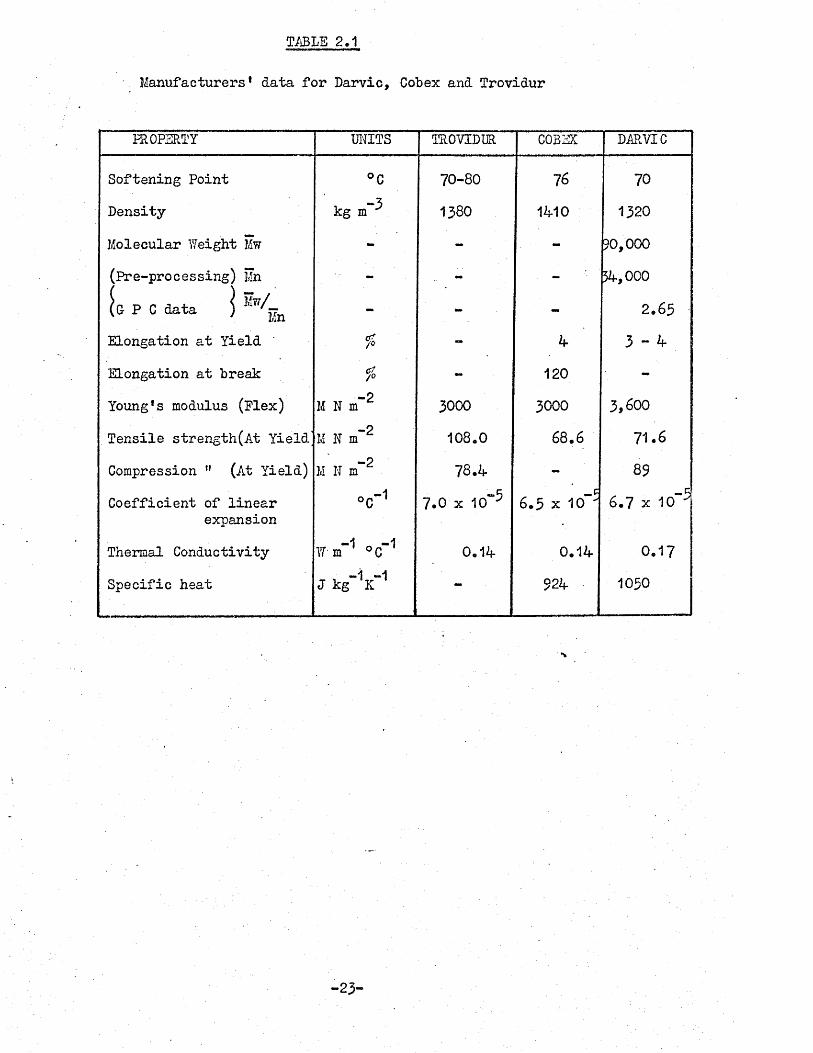
TABLE 2.1

Manufacturers* data for Darvic, Cobex and Trovidur

PROPERTY UNITS TROVIDUR COBEX DARVIC

Softening Point °C 70-80 76 70Density- -3kg m 1380 1410 1320

Molecular Weight Mw - - - 50,000

(pre-processing) Mn [& P C data ] MW/i n a.

54,000

2.65Elongation at Yield /° 4 3 - 4Elongation at break c?7° - 120 -Youngfs modulus (Flex) M N m~ 2 3000 3000 3,600

Tensile strength(At Yield' M N m”2 108.0 68.6 71.6

Compression " (At Yield)Coefficient of linear

expansion

M N m“2

° c ~178.4

7.0 x 10"5 6.5 x 10""89

6 .7 x 10~*

Thermal Conductivity- -1 -1W m °C 0.14 0.14 0.17Specific heat -1 -1J kg K - 924 1050

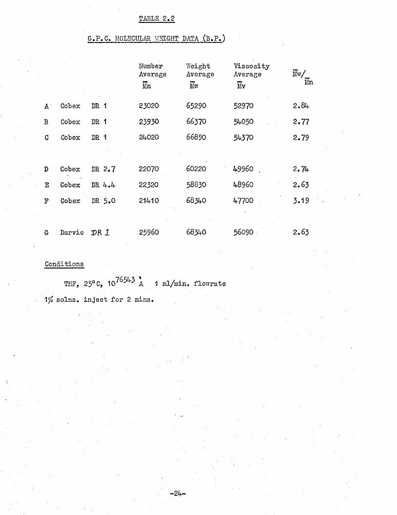
TABLE 2.2

G-.P.C. MOLECULAR WEIGHT DATA (B.P.)

NumberAverage

WeightAverage

ViscosityAverage Mw/_

Mn Kw Mv Mr

A Cobex DR 1 23020 65290 52970 2.84B Cobex DR 1 23930 66370 54050 2.77C Cobex DR 1 24020 66890 54370 2.79

D Cobex DR 2.7 22070 60220 49960 2.74E Cobex DR 4.4 22320 58830 48960 2.63

F Cobex DR 5.0 21410 68340 47700 3.19

G Darvic m l 25960 68340 56090 2.63

Conditions

THF, 25° c, 1 0 ^ 3%A 1 ml/min. flowrate

Vfo solns. inject for 2 mins.

-24-

TABLE 2*3

G.P.C. MOLECULAR. WEIGHT DATA (PSCC)

NumberAverage

WeightAverage

*z*Average 5L/w/

SET AMn

A Cobex DR 1 27320 67800 179700 2.47B ii ii 28070 70220 244350 2.5C ii ii 28350 65800 132600 2.32

D Cobex DR 2.7 27200 67420 155220 2.48E it DR 4*4 28020 66020 157800 2.35F ii DR 5.0 27820 66800 167600 2.40G Darvic

SET B

J)K 1 27250 67670 167600 2.48

A Cobex DR 1 33050 104400 642800 3.16

B ii it 31020 85320 213200 2.75C it it 30250 85970 . 216500 2.86

D Cobex DR 2.7 14650 45576 146200 3.11E tt DR 4.4 27450 • 83570 232700 3.04F n DR 5.0 27500 80920 212800 2.94G Darvic DK X 16900 49800 642800

■ s

2.95

ConditionsTHP, 24°C, 1 ml/min. flow rate, 0*2^ solns* 2 min. injection.

Set A 100-350-A; 700-2000 A; 5 x 105 - 1*3 x 11^ A; 7 x 105 - 5 x 106 A;Set B 700-2000 A; 1.5 x 104 - 5 x IQ21* A; 7 x 105 - 5 x 106A; 5 x 106 - 107A

-25-

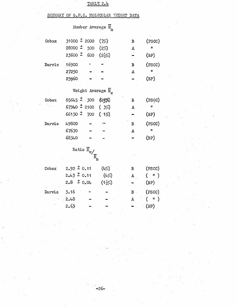
, TABL.B 2.4

SUMMARY OP &.P.C. MOLECULAR WEIG-KT DATA

Number Average M n

Cobex 31000 - 2000 (jfi) B (PSCC)28000 - 300 (2 ) A w23600 i 600 ( & Q - (BP)

Darvic 16900 - B (PSCC)27230 - - A ”23960 - - - (BP)

Weight Average MwCobex 85645 - 300 B (PSCC)

67940 ± 2100 ( 3 $ A "66150 ± 700 (.1$ - (BP)

Darvic 49800 - ~ b (PSCC)67670 A "68340 - - (BP)

Ratio M / w/.

Cobex 2.92-0.11 (kfi) B (PSCC)2.43 - 0.11 (4$ A ( " )2.8 ± 0.04 (l^o) - (BP)

Darvic 3*16 - - B (PSCC)2.48 - - A ( « )2.63 - - - (BP)

-26-

x10

Figure 2,1 G-.P. C. Chromatograms of as-received Cohex sheet.Three samples randomly cut from the sheet.

-t CM ois;oH

-27-

MOLECULAR

WEIGHT

Figure 2.2 G-.P. C. Chromatograms of as-received Darvic and Cobex Sheet

vo

m

oo

CM ooHQ

-28-

Figure 2.3 G-.P. C. Chromatograms of oriented Cobex.Samples with draw ratios of 1, 2.7, 4*0 and 5*0 are shown.

o

-29-

MOLECULAR

7/EIGHT

Figure 2.4(a) G-raph of density of samples of oriented Cobex with excess stabiliser plotted against clarity. The point of on-set of stress-whitening has been arrowed. The draw ratio and the drawing temperature (Tp) have been indicated on the graph.

DensityKgm^

132 0 kAX

130C

j f '

128C

126c

Cobex Fxcess Stabilispr Onset of WhiteningI

DR t*o 0

a :- 1 -

xs- 1 .73 50O : - 2 .3 60X : - 1.1 20

1.1 30

ClearClarity

Opaque

Figure 2.4(b)G-raph of the density of the sample of Cobex plotted as a function of draw ratio.

Cobex Onset of Whitening

DensityKgm"3

1300

1230

Draw Ratio

-30-

Figure 2.5 A typical curve obtained for Darvic using the differential-scanning cgiorimeter cell on the

Du-Pont D.T.A. controller

OXLU

.tI

ooUJ

100Temperature °C

Figure 2.6 A typical curve obtained for Darvic on the thermo­mechanical analyser cell used in conjunction with the Du-Pont D.T.A* temperature controller. The sample was Darvic.draw ratio 1.0.Test direction was the

ProbeDisplace'

ment

+60-<J

Temperature °C

-31-

CHAPTER THREE

EXP3RIM5NTAL TECHNIQUES3.1 Introduotion

In this chapter, details of the equipment used and the experimental methods applied in the preparation and mechanical testing of the oriented PVC samples will he presented. The ultrasonic test method, theory of the method and equipment have been grouped together in section 3*5«

3*2 Equipment

Most of the work was carried out on an electronic recording tensile testing machine; it was an *S! type tensometer, with 2300 kg load capacity, manufactured by Monsanto Tensometer (Slough) (formerly Tensometer (Croydon) Ltd.). It had a specially extended crosshead stroke of 1800 mm, and a continuously variable crosshead speed drive.Drive speed fange was 0,01 mm/minute to 200 mm/minute, produced by two sjoichronous motors coupled by a switching gear box and electronic clutch to the crosshead drive screws. Load ranges gave full scale deflections (f.s.d.) from 2 kg. to 2300 kg. by means of three load cells and electronic switching. Calibration was automatic* and when checked by static weighing, it was found to be within the limits (£ 2%) quoted by the manufacturers (Grade 1A, B.S.I. No.1610 Calibration).Load measurements could be determined to 2 parts in a 1000 from the chart, so that the load values were determined to - 2,2% provided-a suitable f.s.d. range was selected. Ranges could be changed during test, as an electronic tare was used to suppress the grip and sample weights. The chart was run either at a constant ratio to the crosshead, or at a constant speed. It was usually run at constant speed so that the stress relaxation of the sample was recorded after the crosshead had stopped. An event or ‘pip* marker was used to relate positions on the.

load extension curve to events observed on the specimen or when a

-32-

particular frame was exposed while photographing the sample*

.An environmental chamber (hot box), manufactured by Sondes Place Research Laboratories Ltd., was available to fit to the tenso­meter, below the crosshead. The load cell was connected to the samplevia extension rods. The maximum available height of the box was 800 mm. Heating was provided by hot air heated by 3 kW black heat coils and circulated by a high capacity fan; the temperature control was by a Eurotherm thyristor proportional controller; the temperature sensor was a thermocouple monitoring the circulated air. The temperature range of the hot box was -100°C to + 2 7 5 ° The temperature distribution and control over a period of three hours was examined using a Solartron data logging system to record the temperature registered by thermocouples placed at various positions in the chamber. The temperature stability was found to be - 0.1°C and the positional temperature variation was - 1.0°C. Below ambient temperatures were obtained by injecting liquid nitrogen from a thermally pressurised Dewar into the chamber where it vaporised and was dispersed by the fan. The valve was of an on/off type, and tended to stick when ice formed on the valve; this caused the temperature stability at -50°C to be - 3°C.

An optical path through the vertical tensile axis (i.e. throughthe sample) was specially provided, so that visual measurements of the birefringence of the samples could be measured, during the drawing and cooling sequence. Plane polarised light was passed through the aperture in the back wall of the hot box; and analysed using the analyser and an Ehringhaus rotary calcite compensator and binocular viewer, mounted in the head of the Zeiss microscope mounted in front of the hot box (Figure 3*1 )• For room temperature measurements of birefringence, the head was mounted on the Zeiss photopol microscope. The Ehringhaus compensator could be used to determine the retardation ini birefringent

-33“

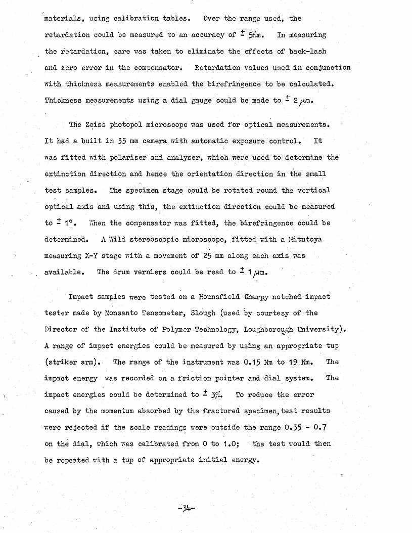
materials, using calibration tables. Over the range used, the retardation could be measured to an accuracy of - 5ftm* In measuring the retardation, care was taken to eliminate the effects of back-lash and zero error in the compensator. Retardation values used in conjunction with thickness measurements enabled the birefringence to be calculated. Thickness measurements using a dial gauge could be made to - 2yum.

The Zeiss photopol microscope was used for optical measurements.It had a built in 35 mm camera with automatic exposure control. Itwas fitted with polariser and analyser, which were used to determine theextinction direction and hence the orientation direction in the smalltest samples. The specimen stage could be rotated round the verticaloptical axis and using this, the extinction direction could be measured

|to - 1°. Y/hen the compensator was fitted, the birefringence could be determined. A YYild stereoscopic microscope, fitted with a Mitutoya measuring X-Y stage with a movement of 25 mm along each axis was available. The drum verniers could be read to - 1 yum.

Impact samples were tested on a Kounsfield Charpy notched impacttester made by Monsanto Tensometer, Slough (used by courtesy of theDirector of the Institute of Polymer Technology, Loughborough University).%A range of impact energies could be measured by using an appropriate tup (striker arm) . The range of the instrument was 0.15 Nm to 19 Nm. The impact energy was recorded on a friction pointer and dial system. The impact energies could be determined to - 3/£* To reduce the error caused by the momentum absorbed by the fractured specimen, test results were rejected if the scale readings were outside the range 0.35 ~ 0*7

on the dial, which was calibrated from 0 to 1.0; the test would then be repeated with a tup of appropriate initial energy.

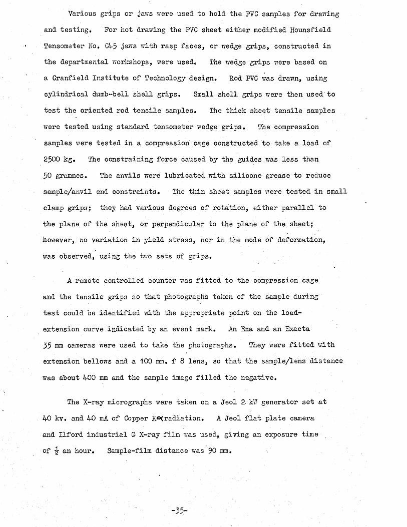
Various grips or jaws were used to hold the PVC samples for drawing and testing. For hot drawing the PVC sheet either modified Hounsfield Tensometer No, C45 jaws with rasp faces, or wedge grips, constructed in the departmental workshops, were used. The wedge grips were based on a Cranfield Institute of Technology design. Rod PVC was drawn, using cylindrical dumb-bell shell grips. Small shell grips were then used to test the oriented rod tensile samples. The thick sheet tensile samples were tested using standard tensometer wedge grips. The compression samples were tested in a compression cage constructed to take a load of 2500 kg. The constraining force caused by the guides was less than 50 grammes. The anvils were lubricated with silicone grease to reduce sample/anvil end constraints. The thin sheet samples were tested in small clamp grips; they had various degrees of rotation, either parallel to the plane of the sheet, or perpendicular to the plane of the sheet; however, no variation in yield stress, nor in the mode of deformation, was observed, using the two sets of grips.

A remote controlled counter was fitted to the compression cage and the tensile grips so that photographs taken of the sample during test could be identified with the appropriate point on the load- extension curve indicated by an event mark. An Sxa and an Fxacta35 mm cameras were used to take the photographs. They were fitted withextension bellows and a 100 mm. f 8 lens, so that the sample/lens distancewas about 400 mm and the sample image filled the negative.

The X-ray micrographs were taken on a Jeol 2 kYT generator set at 40 kv. and 40 mA of Copper K©(radiation. A Jeol flat plate camera and Ilford industrial G X-ray film was used, giving an exposure time of -g- an hour. Sample-film distance was 90 mm.

-35-

3*3 Preparation of oriented material and test samples3.3.1 Drawing of Rod and Sheet PVC

The drawing procedure was essentially the same for all the samples; appropriate grips being used in each case.

Thin sheet (0.3 cun, as-received) Cohex was cut with a knife intorectangular strips 100 mm wide. The gauge length was adjusted togive the required nominal draw ratio, using the maximum availableheight of the hot box, hence the maximum amount of oriented PVC wasobtained. Shaped samples were not necessary for draw ratios lessthan 3.5. For larger draw ratios, shoulders were required to stopthe sample tearing at the grip edge. The side surfaces were polishedwith fine emergy cloth to remove flaws. Thick sheets (5.3 nma) wereprepared in a similar manner, but the blanks were cut on a handsawand were then, polished. The rod samples were turned on a lathe tomake shoulders to fit the Kounsfield shell grips. To reduce thetendency of the thin sheet to slip from the jaws, emery cloth wasplaced between the grip faces and the sample when using the C&-5 grips.For the thick sheets, the wedge grips were necessary because the fixedseparation of the jaws enabled the sheet to slip as it thinned withincreasing extension. For the thick sheets the wedge sheet gripswere very effective because part of the sheet formed a ’’wedge” ofmaterial on the far side of the jaw faces. Samples that slipped

V^sult-eoL inwere not re-used, since to do so would havej^oriented sheets with a non-standard preparation cycle. As the matez-ial pulled out of the jaws during extension, the effective initial gauge length changed, so the sheets were marked with a 5 x 2 mm grid, using an ink stamp. The draw ratio was then determined from grid deformation.

Samples were positioned in the hot box in pre-heated jaws and conditioned at the test temperature, usually 80°C (1 hour for thick

-36-

sheet; 15 minutes for thin sheet). Then the screw.adjuster on the jaws was retightened so that the softened PVC was securely held in the jaws. The crosshead speed of 50 mm per minute was used for a 100 mm gauge length sample, and it was adjusted appropriately for other gauge lengths. The chart was run continuously against a time base. After conditioning, the sample was extended to give the required nominal draw-ratio: the crosshead was then stopped. The sample was held for 10 minutes at the drawing temperature to allow a controlled amount of stress relaxation to occur. The sample was then cooled at constant length, after cooling the sample was removed from the hot box, and the draw ratio and birefringence measured. If the sample was not held at constant length, and allowed to relax: at the drawing temperature, all the extension was recovered.

3.3*2 Characterisation of oriented materialOrientation can be produced in a polymer by many- fabrication

techniques such as extrusion, injection moulding, blow moulding or rolling. The mechanical properties of an oriented polymer will be anisotropic to an extent depending on the degree of molecular alignment. Basically orientation can be introduced by deforming the polymer solid or melt by compression, tension or shear forces. The material used in this work was oriented in a controlled manner by hot drawing sheets of PVC as described in the previous section.

A measure of the degree of orientation could be determined by many different techniques such as draw ratio, x-ray, retraction, nuclear magnetic resonance, or birefringence. Bach method could be used for some specific cases but no method was universal and the measurement was often quite an indirect one. The two methods used in this work were the measurement of draw ratio and birefringence.

-37-

Draw ratio (sometimes referred to as elongation ratio), is defined as the ratio of final length to initial length. This method has been the most widely used technique, as it simply utilizes surface geometry changes. The assumption of affine deformation was made, namely that the surface deformation was the same as the volume deform­ation, and also that no volume change occurred. This technique could be applied to any solid deformation where the initial and final sample dimensions could be compared, e.g. vacuum forming, shear and tensile deformation and rolling. The limitations of this method were that the same draw ratio obtained at different temperatures or strain rates would give different states of orientation. Yield stresses in the draw direction for samples of the same draw ratio, but drawn at different temperatures, have been plotted in figure 3*2. The samples drawn at lower temperatures have higher yield stresses and thus indicate higher molecular alignment. A second limitation was that the initial sample length of a fabricated sheet, might not be that of a completely isotropic polymer. The sheet could be annealed and any retraction noted, but this procedure would not always be practical.

The second method used the optical properties of the polymer molecules. The refractive index or the velocity of light passing through the molecular chains varies and exhibits either a maximum along the axis of the chain and a minimum across the chain axis, or vice versa, depending in detail on the polarisability of the side groups of the molecule. The difference in the refractive indices was called the maximum birefringence of the polymer. In general, an isotropic polymer has a random array of chains and would give zero net birefring­ence. As the orientation was increased, the net birefringence increased. The limitations of this technique were that it could only be used on an optically transparent polymer; and another limitation which would apply

-38-

in the general case but not in the hot drawn sheet was that it gave an average of the value through the sample thickness. Injection moulded samples often have a highly oriented skin surface layer, with a fairly isotropic centre, the birefringence would, ho?;ever, give an average of the two extreme values. The draw ratio and birefringence of the Cobex and Darvic were measured. The non-uniform ends of each drawn sheet were then discarded. The birefringence, being the more funda­mental, was the most useful measurement. The experimental relationship between draw ratio and birefringence for three drawing temperatures of 70°, 80° and 90°C have been plotted in Figure 3*3* The higher values of birefringence for lower drawing temperatures for a given draw ratio can be seen.

The oriented sheets were thought to be transversely isotropic since the contraction-ratio of the width and thickness of the sheet were the same. Further evidence for this was provided by some wide angle x-ray micrographs taken of the oriented PVC and the ultrasonic wave velocities in the oriented PVC. In general, x-rays were not very useful for PVC because of its low crystallinity; however, flat plate camera micrographs showed a broad 'amorphous halo* for the isotropic PVC: micrographs of the oriented PVC were taken along the x and z axes. The micrograph taken along the x axis showed the halo splitting into arcs indicating aligned or oriented 'crystallite* areas: the micrograph along the z axis was similar to the isotropic picture showing that transverse isotropy remained. The micrographs have been shown in figure 3*4*

The ultrasonic measurements also showed that these wave velocities in the xy plane of the drawn sheet were independent of direction and so the polymer sheet was transversely isotropic • Rather than repeat the discussion in detail here, the full discussion can be seen in section 3*5*

“39-

3.3*3 Sample preparationThe uniform section of the drawn sheet was determined by measure­

ment of its draw ratio and birefringence. Samples for testing were then cut from the uniform sections of the sheet or rod3. Thin sheet tensile pieces were stamped out of the sheet, using a Wallace hand press and a dumbbell cutter. Sample gauge length was 6 mm, width 1.5 ioni. extent of the damage to the edges could be seen when samples were examined under polarised light on the Zeiss microscope, Figure 3*5; was about 13/2 of the sample width. The Zeiss microscope was used to measure the angle between the tensile axis of.the sample and the hot draw direction (or axis of orientation). This angle could be determined to - 1° (See figure 3*6). The hot draw direction was identified by finding the extinction direction which could be observed by using crossed polarising filters. Test samples were cut at 15° intervals between }\ = 0° and 50° (figure 3*7a.).

Hod samples were machined into dumbbells on a lathe and small dumbbell shell grips were used to hold the samples during testing. Typically, gauge lengths of 10 mm and diameters of 5nim were used. The ends of the rod compression samples were also machined on the lathe, to provide smooth parallel sides. Sample heights of 6, 8,. 10 mm were used. Silicone grease was used to lubricate the anvil-sample inter­face (Figure 3*7c).

Rectangular bars were first cut from the thick sheet at appropriate angles ^ using a miniature circular saw. Then thick sheet tensile samples were either shaped on a horizontal milling machine, or on a Stanley router; typically the sample was 15 nna long and 3 mm wide.The router was mounted in a sound-proofing box with a horizontal work­table and with a vertical cutting blade. The sheet compression samples were also cut on the miniature saw (Figure 3* 7c). Samples were cut

to give a square section the thickness of the drawn sheet. Sample heights were adjusted to lie ‘between-'the ratio values of thickness/ length 0.5 to 1.0 (kef. 2 Johnson & Mellors). The ends of the samples vrere polished on a metallurgical wet polishing table. Four grades of carborundum paper were used.

Impact bars were prepared by the same method and then notched either -on a milling machine or in a HamsPield notch cutter. Samples were 50 'inm' long, 6 .4 mm wide, and thickness was dependent on the draw ratio. The ultrasonic test pieces were cut as parallelopipeds with sides of 10 mm, 10 mm and the sheet thickness (3-5 mm). The edges of the parallelopipeds were parallel to the x or (1), y or (2) and z or (3) axes. The z or (3) axis was the orientation axis, the x or. (1) was the width of the drawn sheet direction, and the y or (2) axis was the thickness of the sheet direction (Figure 3*13)v

3.4 Mechanical Testing 3*4.1 Tension testing

The dumbbell shaped tensile test pieces were tested mainly at a temperature of 20 - 1°C and at a strain rate of 100/ per minute (10 mm per minute crosshead speed; 10 mm gauge length). The temp­erature was maintained by the hot box running with the cooling attachment fitted, only small adjustments of temperature were required as ambient temperature was nominally 20° C. Care was taken to align samples axially in the grips with respect to the tensile test direction* The samples were extended until a load drop, slope change, or fracture of the test piece was observed on the chart recording of the load extension trace. The event marker was used to identify the point on the load extension curve where the onset of band formation was observed. Thin sheet test pieces tended to slip out of the small grips. This tendency was reduced by glueing emergy cloth to the smooth jaw faces.

-41-

Thick sheet test pieces were tested under similar conditions. The standard Hounsfield wedge jaws were used to hold the samples; slipping was only found to be a problem when testing at a temperature below -30° C, where the additional hardness of the PVC and ice formation, caused difficulties. Sample dimensions were measured before testing and just after the yield point, using a micrometer. Dimensions were measured to 0.005 mm* The thin sheet samples cross-sectional areaof 1 sa. mm or less was determined to about - 3/5* The thick sheetsamples with a cross-sectional area of greater than 4 sq. mm weremeasured to an accuracy of better than - 1/.

3*4.2 Compression testingThe compression samples were tested under the same conditions as

the tensile samples. Compression tests did not suffer from sample slipping problems, nor from fracture before yielding failure. There was one problem: that of the end constraints at the anvil-sample contact surfaces. This was reduced by lubricating with silicone grease and then applying a correction to the measured yield stresses. Samples of three different heights were tested; such that the height to width ratios were between 2.0 and 1.0; samples with ratios greater than 2.0

were liable to buckle. The yield stresses were then plotted against reciprocal length. The unconstrained (or infinite length) yield stress was then obtained by extrapolation to zero reciprocal length (Figure 3.8). (Johnson & Mellors, (2)). Hdward at al. (41) have also reported using a similar technique.

3*4.3 Impact testingThe impact test was the Charpy test, using a Hounsfield instrument.

The sample was supported at both ends but was not clamped. A range of seven tups were available to alter the impact energy. If the sample

—42—

failed to fracture or gave an invalid answer by being outside the dial range 0,35 “ 0.7, a fresh sample was used with a tup of appropriate energy. Dial readings outside the range 0.35 - 0.7 indicated that the fractured sample had absorbed energy, and had dissipated it as momentum rather than in the fracture process. Some tests were made on unnotched samples; but mainly the samples were notched, with a notch radii of 0.23 mm# The sample dimensions were measured and used to normalize the values, as suggested by Vincent (33)* He found that provided the corrections were fairly small, the impact energies were independent of test sample geometry.

3*4.4- Strain measurementsThe method used to measure strain in the sample during test was to

print a grid of dots onto the specimen and measure the spacing of the dots before and during deformation, using photographic negatives of the sample taken at intervals during the test. Sxtensometers could not be used, in general, because of the small size of the test samples. Overall sample dimensions were, however,.measured with a micrometer before and after each test. The photographic method enabled the strain at yield and local strain variations to be determined, whereas an extensometer

• Nwould give a continuous average strain.

35 mm. still photographs were taken at about one second intervals during the testing of a sample. A four digit reference number was

irecorded in each frame, and a corresponding pip mark recorded on the load-extension curve was identified with the same number. The transparent samples with a black grid of dots printed on the surface were difficult to illuminate so as to obtain good contrast. Illum­ination was provided by a 12 volt high wattage lamp that could be focused onto the sample. The grid printing technique developed by Hinton (13) was used. Samples were cut from the sheet and prepared

for testing and then individually printed. Care had to be taken tomount the samples to ensure uniform marking and prevent damage to thesample. The mounting was firm but flexible to allow the metal printingblock and the rigid sample to make good contact. The metal printingblock was a newspaper picture half-tone printing block* a. grid ofdots ■ spaced at 133 to an inch. The block was held in a 7/allacehand press after inking. It was inked with black printer*s ink by ahand roller, - supported by two spacers to ensure uniform inking of theprinting block. The negatives, rather than the prints, were used todetermine the values of strain so that shrinkage of the prints and poordefinition of the prints could be eliminated, Figure 3*9. The negativeswere analysed, using a drum vernier measuring stage mounted on a Y/ild -

+microscope; transmitted light was used. A resolution of -1 j,im could be determined on the vernier;the grain size and diffuse edges of the dots only allowed a repeatability of 9^m. The strains were calculated by measuring the spacings of three groups of dots and averaging over a minimum of three repeated readings. The strains of 0.05 could be determined to £ 0.001.

This system using a still camera only allowed frames to be exposed once every second. At the strain rate used, the strain interval between frames was 0.01. The strain at the yield point could thus be

4.m error by up to - .00;?.

Extensometers could not be fitted to the small samples that had to be cut from the oriented sheet, but it was possible to test a large sample of isotropic Darvic with a strain gauge extensometer fitted to an Instron tensile test machine at Loughborough University. Using the strain gauge, the strain to yield was found to be 4.1 - 0.1 fo strain.By the photographic technique, it was 6 - 1^, (Figure 6.1a & b.). Measurement of sample dimensions after yield for small strains such

-44-

as these would be in error because of the relaxation caused by the large local deformation of the deformation band.

3*5 Ultrasonic Testing 3.5*1 Introduction

The velocities of ultrasonic »/aves propagating in samples of oriented FVC were measured. The elastic constants of the PVC were then derived from the velocity measurements,- The measurements of the ultrasonic wave velocities of the PVC were made, using the equipment at the National Physical Laboratory (by courtesy of Mr, M. F. Markham). Basically, the technique comprised the measurement of -the transit time of an ultrasonic pulse (5 MHz) transmitted through water to a receiver. The Change in transit time (measurable to - 1 ris) was measured when a sample of FVC was placed so that the pulse traversed the sample. The change in velocity with a change in propagation direction was measured and the velocities of the wave through the PVC v/ere calculated. The theory relating the elastic constants and the wave velocity has been outlined belo?/.

3.5*2 Theory of MethodThe theory of elastic wave propagation in anisotropic solids has

been derived by Musgrave (1, 18, 19). For a material that was elastically isotropic in the xy plane, which is the plane perpendicular to the draw direction z, then the stiffness constants for the material are:-

11 C12 C13 0 0 0

CMO

C11 C13 0 0 0

C13 C13 C33 0 0 0

0 0 0 ' ' V 0 0

0 0 0 0 0

0 0 0 0 0 i(c

.45-

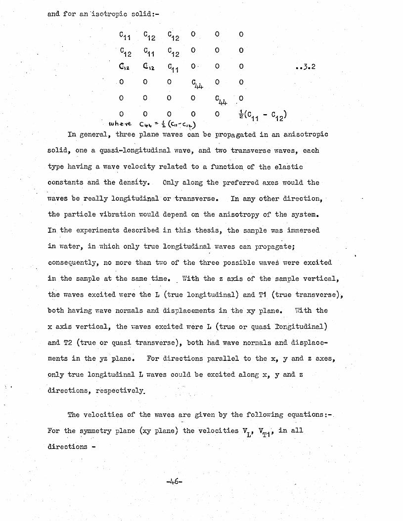
and for an'isotropic solid:

C11 C12 C12 0 0 0

C12 C11 C12 0 0 0C» i C11 0 0 0 ..3.20 0 0 V 0 o0 0 0 0 V•iff * 00 0 0 0 0 *(ci i - V .•£ (c„ - c,z.)

In general, three plane waves can be propagated in an anisotropic solid, one a quasi-longitudinal wave, and two transverse waves, each type having a wave velocity related to a function of the elastic constants and the density. Only along the preferred axes would the waves be really longitudinal or transverse. In any other direction, the particle vibration would depend on the anisotropy of the system.In the experiments described in this thesis, the sample was immersed in water, in which only true longitudinal waves can propagate; consequently, no more than two of the three possible waves were excited in the sample at the same time. Y.rith the z axis of the sample vertical, the waves excited were the L (true longitudinal) and T1 (true transverse), both having wave normals and displacements in the xy plane. Td.th the x axis vertical, the waves excited were L (true or quasi longitudinal) and T2 (true or quasi transverse), both had wave normals and displace­ments in the yz plane. For directions parallel to the x, y and z axes, only true longitudinal L waves could be excited along x, y and z directions, respectively.

The velocities of the waves are given by the following equations :- For the symmetry plane (xy plane) the velocities V^, V^', in all directions -

-46-

where 0 = sample density ; suffices L and T1 are defined in the above text.yz plane with the wave normal at angle R to y axis

P VL2 = i d C33 (C33 - C^) Cos 2 R + P) .. 3.5

P T2 = i & ^33 + + C2,4 “ i ( C33 _ Oos 2 R - P) .. 3.6

P = f [i c33 - i + (U - i c33 - i C^) Cos 2 R.) 2 +

f(C13 + C^) Sin 2 l ) 2j 8 •

For wave normals in the y direction

^ P = C1'1 ~ ° W C11 °44 and thus

e vL2 = °ii . . 3 .8

For wave normals in the z direction P = ~

° 3 3 > and thus

= C33 ..3.9P can he eliminated from 3*5 +3*6 to give

f ( \ 2 + VT22) = i c33 + i c1 + c33 - Cl1) Cos 2R .. 3.10

o 2Thus for measurements in the yz plane, a graph of P (V +.Vrno')\ L T2against Cos 2R should he a straight line. By subtracting 3*6 and

Because of the small size of the sample, difficulty was experienced in obtaining velocity measurements in the x and z directions. Values of the stiffness constants could be obtained without these measurements as follows, was obtained from equation 3*3 and from equation3*4, using the mean values for V^ and V ^ in the xy plane. The slope of the linear plot equation 3*10> namely - J- (C^ - C-j-j)* then enabled

to be determined, and the intercept at R = 0°, (C^ + gave C; »The intercept at R = 90° (C^ + ) also gave C^y The value ofwas obtained from equation 3*i1* T/here direct measurements of velocity along x, y, z axes were obtained, C^, C ^ could be determined from equations 3*3, 3*8, and 3*9; thus various possibilities of checking for self consistency existed.

3.3*3 Ultrasonic equipment' A schematic diagram outlining the essential features of the

ultrasonic tank can be seen in figure 3*16* The axially alignedtransmitting and receiving transducers were mounted in a thermallyinsulated water bath. A 5 MHz ultrasonic wave was generated witha pulse rate of 1 KH • The temperature was accurately maintainedzto **"- 0.1°C by circulating temperature controlled water. This accuracy of temperature control was necessary as the velocity of ultrasonic waves through water varied rapidly with temperature (change of 0.23 metre per second for + 0.1°C at 20°C). The water acted as an accoustic link between the transducers and transmitted only quasi longitudinal waves; ?rater and other fluids do not transmit transverse waves. Measurement of the transit times of the ultrasonic waves were made by introducing calibrated delay into the measurement circuit to bring the signal back to the reference point. Measurements could be made to - 1 nanosecond. The arrival times and sample dimensions were used to calculate the velocities. The pulse form can be seen in figure

- .8-

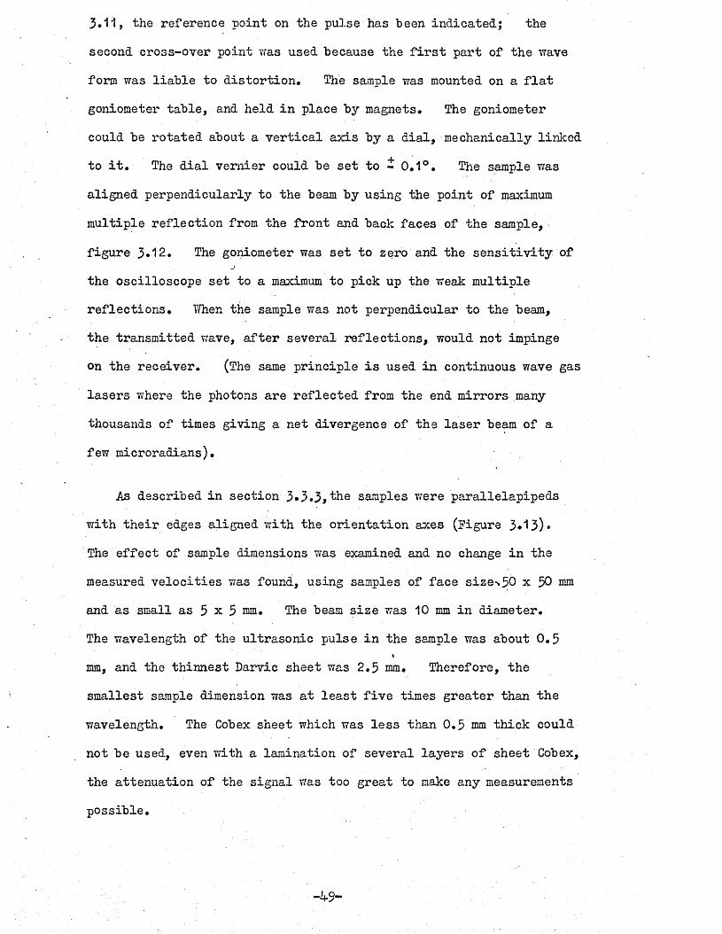
3.11, the reference point on the pulse has been indicated; the second cross-over point was used because the first part of the wave form was liable to distortion. The sample was mounted on a flat goniometer table, and held in place by magnets. The goniometer could be rotated about a vertical axis by a dial, mechanically linked to it. The dial vernier could be set to i 0.1°. The sample was aligned perpendicularly to the beam by using the point of maximum multiple reflection from the front and back faces of the sample, figure 3*12. The goniometer was set to zero and the sensitivity of the oscilloscope set to a maximum to pick up the weak multiple reflections. When the sample was not perpendicular to the beam> the transmitted wave, after several reflections, would not impinge on the receiver. (The same principle is used in continuous wave gas lasers where the photons are reflected from the end mirrors many thousands of times giving a net divergence of the laser beam of a few microradians).

As described in section 3 * 3 . 3 , samples were parallelapipeds with their edges aligned with the orientation axes (Figure 3*13)*The effect of sample dimensions was examined and no change in the measured velocities was found, using samples of face sizesfjO x 50 nrn and as small as 5 x 3 mm. The beam size was 10 mm in diameter.The wavelength of the ultrasonic pulse in the sample was about 0.5

i

mm, and the thinnest Darvic sheet was 2.5 mm. Therefore, the smallest sample dimension was at least five times greater than the wavelength. The Cobex sheet which was less than 0.5 mm thick could not be used, even with a lamination of several layers of sheet Cobex, the attenuation of the signal was too great to make any measurements possible.

-49-

3*5*4 Test procedure, calculation of velocities, and velocity results

The arrival times of.the pulsed wave through the water was measured, the specimen was then mounted and the change in transit time through the sample was recorded. The sample was positioned and then the temperature was allowed to return to 20° C before any measurements ?;ere made. Readings of the transit times were taken at 5° intervals of rotation about a vertical axis. The quasi­longitudinal waves were measurable for angles of incidence over the range 0° - 35° > corresponding to angles of refraction R of 0° - 60°. The quasi-transverse waves were measured over the range 25° - 85° which corresponded to angles of refraction 15° ~ 51 °, :>-A- The transit times were measured for two sample positions, that of the z axis vertical giving particle displacement in the xy plane, and the x axis vertical giving particle displacement in the 2y plane. The arrival time through the water was checked between any repositioning of the sample, and appropriate values used to calculate the velocity through the water.

The velocities of the transverse and longitudinal waves were calculated from the measured changes in transit time between the transmitter and receiver as follows. At normal incidence, the longitudinal wave velocity was given by equation 3*12

where VT = longitudinal wave velocity in the sampleJuVw longitudinal wave velocity in the water

difference in arrival times of wave throughwater and through water and sample

d thickness of sample

-50-

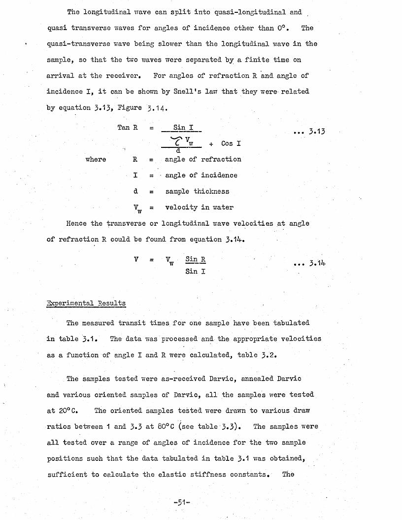
The longitudinal wave can split into quasi-longitudinal and quasi transverse waves for angles of incidence other than 0°. The quasi-transverse wave being slower than the longitudinal wave in the sample, so that the two waves were separated by a finite time on arrival at the receiver* For angles of refraction R and angle of incidence I, it can be shown by Snell*s law that they were- related by equation 3*13> Figure 3.14.

Tan R = Sin I ... 3.13C \ + Cos I

— ~a— —where R = angle of refraction

I = angle of incidenced = sample thickness

= velocity in water Hence the transverse or longitudinal wave velocities at angle

of refraction R could be found from equation 3*1 -*

V = V Sin R • ,,w 111 1 j •••Sin I

Bxperimental Results

The measured transit times for one sample have been tabulated in table 3«i* The data vras processed and the appropriate velocities as a function of angle I and R were calculated, table 3*2*

The samples tested were as-received Darvic, annealed Darvic and various oriented samples of Darvic, all the samples were tested at 20°C* The oriented samples tested were drawn to various draw ratios between 1 and 3*3 at 80°C (see table-3*3)* The samples were all tested over a range of angles of incidence for the two sample positions such that the data tabulated in table 3*1 was obtained, sufficient to calculate the elastic stiffness constants* The

variation of the velocities with angle R for sampleDR 3*3 have been plotted in figure 3*16* The longitudinal velocity change with draw ratio along the z axis has been plotted in Figure 3,17 and tabulated in table 3»3» The anisotropy of the velocity in the plane perpendicular draw to the direction was found to be 0.80 5 and between the z and x axis the maximum anisotropy measured was

The velocities were used to calculate the sample elastic stiffness and compliance constants; the theory given in the previous section was used to determine the stiffness constants and the compliance constants were then found by applying the matrix transformation, the relationship between the constants have been given below in equation 3*15*

S., = C11 + C1233B

2= C11 C33 ~ °1311

m ... 3.15S12 = C132 - C1 2 C33

AB

S13 “ ~C13B . '

V = V ~ S66 = ;i- = .— - J L —

where A = (C^ - C12)

B = ^C11 C33 + C12 C33 " 2 C13 ^The velocities of the longitudinal wave in the x and y direc­

tions were equal within 0.8£c, Table 3*1/ an& so justified the earlier assumption that the drawn sheet was transversely isotropic. It was estimated that random errors in the velocity measurements lead to uncertainties of about ~ 0.4yc in and - 3*Ofo in the values of the

-52-

other constants* The random errors in the density measurements contributed another - 0.7/S to the uncertainties. • The differences between values of elastic constants measured on nominally similar samples were about 3/2* The measured value of annealed samples remained unchanged, indicating that the samples in the as-received state were isotropic. The temperature stability was such that measurements of the velocity through the water over the period oftest of one sample was - 0.1 fo. A graph for one of the samples,

2 2of + V^2 f plotted against cos 2 R for directions in the yz plane has been shown in figure 3*15* The graph which, according to equation (3*10), should be a straight line indicated the internal consistency of the velocity measurements* The stiffness constants obtained from the measurements have been tabulated in table the compliance in table 3*5*

Ultrasonic measurements could not be obtained for the Cobex material because of total attenuation of the signal-in the sample.The attenuation was due to the sample thickness of -J- mm or less being about the same order as the wavelength of the ultrasonic pulse in the PVC (wavelength = 0.3 mm). Being careful to avoid altering the sample orientation, it was attempted to laminate several layers of oriented Cobex together, using TKF as a solvent. It proved impossible to eliminate the effect of the interlayer surfaces.Time did not permit further experimentation to laminate using a heat treatment on the isotropic sheet. Darvic sheet, which was prepared by the manufacturers by lamination of calendered foils under high pressure and temperature, did not show any sign of inter­layer surfaces, by attenuation or multiple reflections within the sample.

-53-

TABLE 3*1

ULTRASONIC PULSE TRANSIT TIMES FOR VARIOUS ANGLES OF INCIDENCE

Oriented PVC D.R. 2.5Temperature 20°CSample Thickness 3*216 mm.Water transit time 76.826 /as

ZY Plane XY PlaneAngle of Longitudinal Shear Longitudinal ShearIncidence

(X)° (T)/*s (T) /as (T) yMS (T)/Us0 76.136 - 76.123 -5 76.121 - 76.122 -

10 76.098 - 76.109 -15 76.021 - 76.086 -20 75.962 - 76.053 77.92525 75.812 77.516 76.006 • 77.950

3° 75.571 77*488 75.938 77.98435 75.263 77*470 75.834 77.01140 - 77.441 - 77.05845 - 77*444 - . 77.14950 - 77*477 - . 77.19355 - 77.526 77.26660 - 77.599 - 77.35065 - 77.689 - 77.46210 ' - 77.790 - 77.56975 - 77.817 - 77.68880 - 78.050 - 77.91685 - 78.343 - -

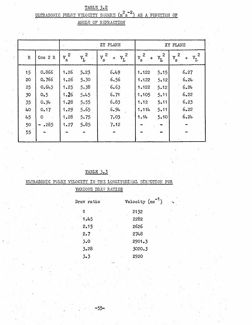
TABLE 3.2ULTRASONIC PULSE VELOCITY SQUARE (m2s~2) AS A FUNCTION OF

ANGLE OF REFRACTION

ZY PLANE XY PLANE

R Cos 2 R

CM

VL22 2

v s + V Vs2 + v 2L2 2

V« +' V TS L

15 0.866 1.26 5.23 6.49 1.1.22 5.15 6.2720 0.766 1.26 5.30 6.56 1.1.22 5.12 6.2425 0.643 1.25 5.38 6.63 1.122 5.12 6.2430 0.5 1.26 5.45 6.71 1.105 5.11 6.2235 0.34 1.28 5.55 6.83 1.12 5.11 6.2340 0.17 1.29 5.65 6.94 1.114 5.11 6.2245 0 1.28 5.75 7.03 1.14 5.10 6 • 2450 - .285 1.27 5.85 7.12 - - -55 mm * **

TABLE 3.3ULTRASONIC PULSE VELOCITY IN THE LONGITUDINAL DIRECTION FOR

VARIOUS DRAN RATIOS—1Velocity (ms )

2132 2282

2626 27482901.33020.3 2920

Draw ratio 11.452.152.73.03.28■3.3

-55-

TABLE 3.4DARVIC 3.5 mm SHEET, DRAW AT 80°CElastic stiffness constants C.measured ultrasonically.Density P = 1390 - 1 kgm~J

-2Stiffness Constants in GNmDraw Ratio Birefringence x 10 c,,11 °12 °13 °33 V

1.00 0.11 6.30 2.77 2.77 6.30 1.801.45 0.78 7.2 6 3.50 3.90 7.62 1.601.75 1.60 7.16 4.16 4.34 9.12 1.682.15 2.01 7.18 4.07 4.79 9.59 1.742.50 2.67 6.95 4.50 4.3 9.75 1.652.70 3.27 6.86 4.46 4.47 10.50 1.753.00 3.45 6.65 3.88 4.43 11.70 1.393.30 3.63 6.68 3.74 4.79 11.85 1.58

TABLE 3*5DARVIC 5.3 mm SHEET, DRAM AT 80°CCompliance constants S.^ calculatedfrom the ultrasonically measured stiffnessconstants C. .. ■ .ij 2 —1Compliance Constants in m (&N)

Draw Ratio Birefringence x 10^ s^ s ^ s ^1.00 0.11 0.217 -0.066 -0.066 0.217 0.5551.45 0.78 0.207 -0.059 -0.076 0.205 0.6251.75 1.60 0.276 -0.097 -0.068 0.173 0.5952.50 2.67 0.269 -0.138 0.058 0.149 O .606

2.70 3.27 0.275 -0.142 -0.057 0.143 0.5713.00 3.45 ... 0.250 -0.111 -0.053 0.125 0.7193.30 3.63 • 0.246 -0.094 -0.062 0.134 0.633

-56-

Figure 3*1 Sketch showing the arrangement for the measurement of birefringence during the hot drawing process in the

environmental chamber

chamberwalls

Extension Rod Sz Jaw

Glass windowlighttube Eyepiece

Polarissr AnalyserI l sampleCompensator

Jaw & Extension RodII I N

-57-

Figure 5»2 Graph of tensile yield stress in the draw direction showing the effect of increasing temperature.

ooON00

0 *p £4 «H -P X CO £

O

CO

-58-

DRAY/

RATIO

Figure 3>3 G-raph showing the effects of orientation and drawing temperature on "birefringence* Plotted points are

experimental data*

o o oCO

oo

CM

0 H1

-59-

Figure '3 A X-ray micrographs showing a) the as-received PVC amporphous halo and b) the splitting of the halo into arcs in the oriented PVC.

Figure 3*5 Photograph showing, by use of crossed polarisers the sample damage due to cutting.

Figure J>.& Diagram defining the angle

Draw direction of the drawn

sheet

sile axis a tensile pie cut at

Ter

Figure 3«7a. (Left) Photograph of strip cut from as-received PVCsheet, 6 mm thick. (Centre) Strip after being oriented by hot stretching. (Right) Dumb-bell tensile and parallel­sided compression test pieces machined from the oriented strip.

- 61-

Figure 3.7b« Sketch of tensile test samples for varioussheet thicknesses.

0=00. 3 & 0.5 mm (thin sheet)

\ r

v .3.0 mm (thick sheet)

5 & 6 mm (thick sheet)

Figure 3.7c Sketch of compression test samples.

L = 8 mm L = 6 mm L = 4 mm

-62-

Figure 3*8 Plot of measured yield stress against reciprocal of compression test-piece length. The corrected yield stress (arrow) was obtained by extrapolation to zero

reciprocal length.

100

YIELDSTRESS

-2MNm

0.150 0.05 0.10 0,20LENGTH “1 mm”1

Figure 3*9 Photograph showing the grid of dots printed on the strain and reference samples. They are mounted

in the compression cage.

-63-

Figure 3.10 Schematic outline of the ultrasonic tank.The sample and transducers are immersed in temperature controlled water.

Transmitter Receiver

<-> RotatingTableElevation

PlanSamnle_ \Rotating

tableTransmitter Receiver

Figure 3*11 Diagram of the ultrasonic pulse waveform. The reference point was taken as the second cross-over; this point was not lost, unlike the initial part of the pulse which was lost because of dispersion effects at different angles.

Figure 3«12 The waveform on the oscilloscope showing the multiplereflection position.

Figure 3*13 Diagram showing the ultrasonic sample related to thex, y and z axes.

Drawdirection

Y (or2)Sheet thick n«-esj

- 65-

Figure 3.1^ Sketch showing the ultrasonic path through the sample.

T - Transverse Wave L - Longitudinal Wave

FromTransmitter

To ReceiverWave Normal •

2 2Figure 3.15 Graph of v^ + v ^ plotted against cos 2R for directionsin the yz plane. V-. and v are the quasilongitudinal and quasi--L 12transverse wave velocities, equations (3.5) ancL (3*6), and R. is the angle between the wave normal and the y axis. According to equation (3.10) this graph should be a straight line.

x10

2 -2 m s

T27.0

6.0- 1.0 0 0.5 1 .0

Cos 2R

- 66-

Figure 3»16« G-raph of longitudinal and transverse velocities plottedagainst angle of refraction R.

(Velocity) Longitudinal

Shearx x

60400 20Angle of refraction R degrees.

Figure 3*17 G-raph of longitudinal velocity plotted against draw ratio.3000

Velocity

ms

2f>00

2100

31 2Draw ratio

-67-

CHAPTER POUR

YI3LDIN& OP ORIENTED POLYVINYL CHLORIDEIntroduction

In the previous chapter, details about the preparation of the drawn sheets of PVC and test samples, cut from the drawn sheets, were presented. Sheets were drawn to different draw ratios, so that a series of sheets with increasing orientation were obtained. Samples were cut from the uniform sections of each sheet, such that the tensile axis of the samples made the required angle ( ^ ) to the molecular chain alignment direction. The degree of orientation was set by the drawing temperature and draw ratio. The degree of orientation was specified using draw ratio and birefringence measure­ments, The oriented PVC samples were then tested in tension and compression, and the stresses at yield were measured. These yield stress results have been reported in this chapter. The results were used to test the predictions of the Hill yield criterion, modified by the inclusion of a 'frozen-in* stress term, that the tensile and compression yield stresses would be different in magnitude.Various properties of the 'frozen-in* stress have also been discussed,

%together with some comments on the possible molecular mechanism for the 'frozen-in' stress.

Tensile samples were prepared from 0.5 mm thick sheets of Cobex. Compression tests could not be made on samples cut from sheets as thin as 0.5 mm, and so PVC with a thicker section had to be obtained. Trovidur PVC was available in rod form, with a diameter of 10mm.This was used for tension and compression tests, but only samples along the draw direction could be prepared from it; also it was only available as a pigmented extrusion. Cobex sheet was not made by BXL as thick sheet, but ICI were able to supply a rigid PVC (Darvic),

-68-

similar to Cobex in properties. The tension and compression samples were prepared from Darvic sheet at various required angles of J\ between 0° and 90°, so that the variation of yield stress with orientation direction was measured experimentally; full experimental details have been given in chapter three.

The true and nominal yield stresses and yield strains were obtained from the fyield point*, on the load-extension curve; the yield point marked the onset of local permanent plastic deformation, usually in the form of a deformation band. The load-extension curve exhibited either a load-drop or a knee at yield. The yield load for this work was defined as the load maximum on the load extension curve, or as the intersection of tangents drawn either side of the knee, which was observed on the load extension curve if no maximum existed, Figure 4.1. Yield stresses were obtained from the yield load by dividing the yield load by either the initial cross- section for nominal stress or the true cross-section for true stress. Hargreaves (8) also used this definition of yield point. The work discussed in this chapter has also been reported elsewhere (Rawson and Rider (38)).

4.2 Yield stress results4.2.1 Tensile yield stresses

The true tensile yield stress of the isotropic as-received Cobex~2was found to be 68.5 MNm- , measured in. the direction that showed a

-3slight positive value of birefringence, A n = 0.11 x 10 ; thisdirection was made the draw direction and designated the Z or 3axis. The perpendicular direction in the plane of the sheet gave

—2a true yield stress value of 60.8 MNm (the X, or 1 axis). The anisotropy was due to the calendering process used to fabricate the

-69-

sheet. Similar anistropy has “been observed in sheets of milled, vulcanised rubber* The Darvic sheet also showed similar aniso-

-3tropy in the as-received sheet* The birefringence was 0*10 x 10 .-2The true yield stresses were 82*5 MNm for the Z axis direction,

and 76*5 MNm for the X axis direction (Table 4*2)

The yield stresses for the series of drawn Cobex sheets were determined; the X = 0° and 90° nominal yield stresses plotted against increasing draw ratio for FVC oriented at the three drawing tempera­tures (70* 80, 90°C) have been shown in Figure if* 2* The measure of anistropy of the nominal tensile yield stresses ((T ) at draw ratio of 3*0 could be seen from the ratio W which was 6*3 drawn at 70°C; 4*5 drawn at 80°C and drawn at 90°C. Some of the samples failed by brittle fracture before any sign of plastic deformation* Details of the fracture behaviour will be discussed in chapter seven* It will be seen from these results that the anisotropy for the same draw ratio was reduced as the drawing temperature was raised. In chapter 3«3«2 it was also seen that the molecular alignment as measured by birefringence for a given draw ratio was less as the drawing temperature increased*

The variation of the nominal tensile yield stress with angle X has been plotted in figure 4*3 and 4*4 for samples drawn at 80°C. Experimental points for draw ratios of 1, 1*5, 1*95* 2*5,.3*0,3*3, 4*5 have been shown* The curves drawn through the experimentalpoints have been drawn as the best fit by eye. The curves crossed

\

the isotropic curve at X = 30 - 2°, showing that the yield stress at X= 30° has. not altered from that of the isotropic value* No minimum value was observed. The yield stress decreased continously with increasing X • The experimental curve for HR = 4* 5 which was stress whitened,did not, however, cross at X = 30°; in

-70-

fact, all the measured values were considerably lower than expected from the progressive change of yield stress with increasing draw ratio. The reason for the lower yield stresses could he connected with the low density of the stress whitened drawn sheet (see section 2.4), as the loss in density occurred by formation of microvoids; thus, the chain mobility could be increased in the whitened sheet and so a smaller stress would be required to produce yielding.

The plastic deformation at yielding occurred in localised deformation bands in both the isotropic and oriented sheets. The bands contained re-oriented material; this was observed as a change in extinction direction when the sample was viewed between crossed polarizing filters. The angles at which the bands formed were measured relative to the sample tensile axis, and the angle iden­tified asXj or by applying the definition given in figure 4.5; Hargreaves (8) also used this definiation of If .

For isotropic samples, the band angles andlQ, were found to be 55-1°• For oriented sheet, the angles X at which the deform­ation bands formed, for angles of \ not equal to 0° departed from

X~1 = 7 2 = 55° • ^he experimental points have been plotted in• *v

figure 4.6 a, b, c, d, for draw ratios of 1.5, 2.0, 2.5 and 3*0« Increasing orientation increased the divergence of IT from 55° for samples with low values of }\ • At high angles of }\ , the valuesof approached the numerical value of the orientation'angle,which meant that the bands were forming nearly parallel to the orientation direction. For samples that failed in fracture, thefracture surface was parallel to the orientation direction. Moredetailed study of the geometry of the deformation bands has not been made in this work, because Hargreaves (8) recently conducted an exten­sive examination of them.

-71-

4.2*2 Tensile and compressive yield stresses in the draw direction

The isotropic Trovidur was tested in both tension and compression* The true compression yield stress was corrected to eliminate, as far as possible, the error introduced by constraints at the anvil surface, caused by frictional contact of the sample ends and the anvils. The anvils were lubricated to reduce this effect as much as possible, and the yield stress was corrected as explained in chapter three: the correction involved extrapolation of the yield stresses from samples of different heights to a sample of unconstrained length.

The true compression yield stress (O') was found to be largercthan the true tensile yield stress (0 .) (table 4.1). The isotropic Darvic samples also gave the seme result (table 4.2). Duckett et al. (30) and Bauwens (48) have both reported similar results. Duckett et al. (30) worked on PP, and measured the ratio of compression to tensile yield stresses. Their ratio was slightly greater than one (the value could not be accurately determined from the published graph in their paper). Bauwens (48) worked on PVC and found the ratio of compression to tensile yield stresses to be 1.3. 3auwens explained the effect as being a result of the compressibility of the polymer and hence that the yield stresses were dependent on hydrostatic pressure. Rabinowitz et al. (45) have published results of extension work on the dependence of torsional stresses of FMMA on hydrostatic pressure. A marked dependence was found.

The oriented Trovidur was tested in tension and compression at various draw ratios; Figure 4 .7 and Table 4.1. The true compression yield stress in the draw direction slowly decreased with increasing orientation, giving a maximum anisotropy of 20% for the draw ratios

-72-

tested. The true tensile yield stress increased rapidly with drawratio such that by a draw ratio of 2.0 the tensile stress exceededthe compression yield stress, and at a draw ratio of 2.5, the ratioof tensile to compression yield stress was 1.6 (C / CT; = 0.6)c

Duckett et al. (30) have independently, reported similar results for oriented PP in which they noted the change of tensile yield: stress from being less than the compression yield stress to being greater than the compression yield stress at a draw ratio of 2.0.

For some metals, the tensile yield stress has been found to be greater than the compression yield stress. The explanation for this has been attributed to a residual stress due to grain boundaries as the yield stresses have been found to be equal for measurements on single crystals. The effect was called the Bauschinger effect. For oriented polymers, the term ’frozen-in* stress has been used to explain the non-equality of the tensile and compression yield stresses. The frozen-in* stress has been attributed to frozen-in retraction stress caused by extending and aligning the polymer chains, which try to return to a random configuration of higher entropy (Hargreaves (8), Bridle et al. (22), Brown et al. (6)).

The variation of the yield stresses of isotropic and oriented FVC, for the draw direction, with temperature and strain rate, were also investigated. The isotropic PVC was tested at a strain rate of 100 c per minute, and the true tensile and compression yield stresses were measured over the temperature range -40°C to +60°C, Figure 4.8. At all temperatures,- the compression yield stress was greater than the tensile yield stress. The full lines in the graph were drawn to indicate that the yield stresses decreased linearly with rising temperature, apart from an apparently anomalously low value of the compression stress at 0°C. For the purpose of later

-73-

calculations, compression yield stresses at OaC and 60°C were obtained by linear interpolation and extrapolation.

Oriented PVC with a draw ratio of 2.5 was used for the yieldstress tests at strain rates of 100/b per minute and 1 . per minute,over the temperature range of -40°C to +80°C. The plotted pointsin figures 4.9 and 4.10 show the measured true tensile and compressionyield stresses where the tensile yield stress exceeded the compressionyield stress for both and lOOfo strain rates. The full lines werenot theoretical, but show the yield stresses decreased linearly untilthe glass transition temperature (T ) of 67°C was approached, indicated

Sur*by a vertical broken line, the drawing temperature of 80°C was also

indicated by a vertical broken line. The yield stresses of the oriented sheet were non-linear as the Tg was approached. It was difficult to measure these yield stresses near Tg because the samples were- placed into a preheated hot box, and then allowed to attain equilibrium temperature before they were tested. Consequently, the heating rate was not controlled and any change of dimensions by the release of the internal stress was difficult to measure. The yield point was difficult to determine because the material was near the transition from a glass to a rubber-like state. To try to obtain further information about the behaviour near Tg, the oriented PVC was examined in the thermo-mechanical probe cell (IMA) and differential scanning calorimeter (DSC) of the Dupont thermal analysing equipment. In these cells sensitive measurements could be made at a controlled heating rate. The yield stress values could, however, not be obtained, only dimension expansion (thermal expansion and any stress relieved expansion) and specific heat changes could be measured together with the softening point tempera­ture. This has been discussed in section 4.4*3*

-74*

4*2.3 Compressive yield stresses

True compression yield stresses as a function of angle (A)were’obtained from tests on oriented sheets of Darvic. Darvic wasused for the various reasons given earlier. Experimental datagiving the true'compression yield stresses (CT ) as a function of ^has been plotted in figure 4.11. The data was obtained from sheetdrawn at 80°C, to various draw ratios. The anisotropy of thecompression yield stresses was quite low compared with that of thetensile yield stress. ' For compression tests the maximum yieldstress anisotropy occurred between the 0° and \ = 45° values.The ratio CT _/ CT , c = 1*30, whereas, the same draw ratio (DR = 3) c,uthe maximum tensile anisotropy 01 _/01T,90 = 4.5* The compressionyield stress variation with (A) showed a minimum at 45° > the = 0°and 90° yield stresses were approximately equal. In figure 4.12,the compression and tensile yield stresses for FVC (Darvic) withthe same draw ratio (DR = 2.5) have been plotted on the same axis.

4.2.4 Drawing and retraction stressesThe load-extension curve recorded during drawing (figure 4.23)

showed a load increase until the crosshead stopped. The stress—2at this point was called the drawing stress (0ffi 'MNm~ ). After the

crosshead stopped the load decreased with time while held atconstant length; on cooling, the stress relaxation was eventuallycounteracted by thermal contraction stresses at which point the

—2recorded load increased. The relaxed stress (CT Mv7m ) was calculated from the load recorded .just before the sample was removed from the jaws, after the sample had been cooled at constant length. The sample retained its extended configuration on being released from the ja?fs, after being cooled to room tempera­ture. On reheating the sample to above Tg the polymer contracted

to recover its original dimension, unless it was constrained in thetensometer jaws. It was observed that the ratio, for drawing at70°C.(T = 60fb CT and for drawing at 90° C, (T = 80% CT ,■*,r * m ° 9 r: m andthat:- 0;(90°C) = <T(70»C). Penny (55) also noted the increasedpercentage stress relaxation for lower drawing temperatures in PS,and he separated the drawing stress into two components, and relatedthe first component, a rapid relaxation which was a function oftemperature, to a bond-bending relaxation, and the second componentto the orientation process.

Birefringence measured for the PVC during drawing increased monotonically while the crosshead was moving. For a drawing temperature of 70°C, the birefringence stopped increasing when the crosshead stopped and remained constant while the load relaxed at constant length and temperature. For 90°C drawing temperature, a small decrease in birefringence (not more than 5/9 observed, and ak120°C a further 5/o decrease was measured. On allowing the polymer to contract, the birefringence returned to within of the starting value, as did the draw ratio. This behaviour would tend to confirm Penny’s model of a two-component stress relaxa­tion. The bond-bending component increases as the temperature was lowered.

Penny (55), working at the Monsanto Chemical Company, has also reported some stress recovery experiments in which the oriented samples of PS were held at constant length and then rapidly heated by powerful radiant heaters. He reported recovery of up to 80% of the maximum drawing stress (CT ) as a stress pulse recorded on a load cell as the PS passed through its Tg. The percentage recovery stresses were very dependent-on the strain rate of drawing, the drawing temperature and the polymer molecular weight.

From these observations, it v/ould appear that the drawing stress and retraction stresses could be equal if the stress relaxed component was allowed for. If the drawing stress had two components; one a molecular aligning component which gave rise to the birefring­ence and a second bond-distortion component, then the bond distortion component could relax without affecting the orientation induced birefringence.

These stresses were measured at or above Tg, with the polymer in a rubber-like state. On cooling to ambient temperature, where the PVC was in a glassy state, various changes occurred, including a reduction in free volume and formation of van der Waals forces, which locked in the orientation stress, leaving the material in a state of unstable equilibrium.Compared to the isotropic polymer, the degree of order due to the orientation could cause a re-'arrange- ment of the free-volume and hence modify the arrangement of van der Y/aals type forces. The effect of these stresses below Tg has been discussed in the next section.

if.3 Discussion of yield stress results 4.3*1 frozen-in* stress

The uniaxially oriented P.V.C. sheet is stable in size at room temperature. However, on heating the polymer to a temperature exceeding the glass transition temperature, the polymer sheet will shrink in the draw direction and expand in the thickness and width directions. The.extended molecular chains are fstablef in the room temperature condition, but which, demonstratably, have an associated strain and stress acting to contract or compress the polymer. This ’stress* at temperatures below Tg has been called the ’frozen-in* stress (a ), in this thesis.

- 77-

Below Tg, the free volume associated with each molecular segment has reduced to such an extent that the molecular backbone segments cannot rotate sufficiently to release the strain, or the stress, and return to the coiled configuration of an isotropic polymer. The oriented polymer has an extended zig-zag chain configuration produced by the drawing process. So below Tg the stress and strain could be thought of as being locked in by the large increase in mechanical or ’thermal crosslinks’ caused by the reduction of the free volume.On the macroscopic scale the polymer is in equilibrium. Yielding of the polymer under uniaxial tension or compression would then occur at a point when the free volume had increased to a critical value, allowing molecular segmental movement. W.Whitney and R. D. Andrews (61) have experimentally measured 0.3/S increase in plastic relative volume (or free volume) in polyvinyl formal at yield in uniaxial compression of the isotropic polymer.

On a molecular scale, this model could be visualized as an extended spring held by wax. Vihen the wax is solid each individual section of the spring is held in place by the opposing force of the wax. If the wax melts, then the spring is free to contract. Neglecting the detailed mechanism, the effect of the ’frozen-in’ stress at yield would be allowed to act by local instantaneous melting of the wax, thus freeing the ’frozen-in1 stress.

The general details of the tensile and compressive yield stress variations can be partly explained by the concept of a ’frozen-in’ stress using this free volume spring and wax model.In the draw direction at yield the ’frozen-in* stress acts to compress the polymer so that in the tensile case the ’frozen-in* stress opposes yield and so the tensile yield stress has to increase in magnitude. In the compression case the ’frozen-in’

-78-.

stress assists yield and so the compression yield stress decreases.

Since yielding involves a gross rearrangement of the molecular segments it is not unreasonable to expect that the ’'frozen-in* stress could be released to act at the yield point or possibly progressively up to the yield point.

In the next section a mathematically based yield criterion, using the concept of ’frozen-in* stress, has been discussed.

4.3*2 Hill yield criterion modified by *frozen-in* stressPreviously Hargreaves (8) 555 and Rider and Hargreaves (10) *,

working on the yield behaviour of oriented PVC, found Hill’s anisotropic yield criterion to be useful in predicting the tensile yield stress variation of oriented PVC in the plane of drawn sheet, equation 4.1. The criterion 7?as put forward by Hill (3) as a form of the Von Ilises criterion applicable to anisotropic materials equation 4.1. The axes 1, 2, 3 have been taken along the principal axes of anisotropy. CT and^were the tensile and shear stress components H, F, G, N, L and M were parameters characterising the state of- the material, which had to be determined experimentally

form of equation 4.2. Transverse isotropy about axis 3; is assumed because of the isotropy of the transverse direction contractions during drawing, and hence G = F.

H (0* - ^22 + "^^22 ”* ^33) ~ +

2 N + 2 I ^ 223 + 2 M = 1 • • •. 4.1

Rider and Hargreaves (10) used this criterion expressed in the

2 2 G Cos A + (G + H) Sin*" A + 2 (M - G) Sin2 A Cos2 Aj = 1... 4.2

* In references- 87To739« The symmetry axis was the x axis, hence equivalent Kill parameters were then F, H, and N respectively.

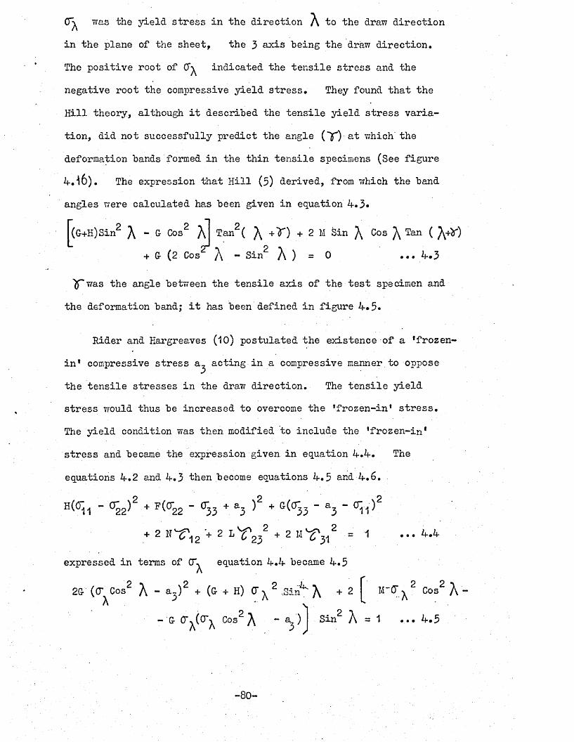
CT was the yield stress in the direction A to the draw direction in the plane of the sheet, the 3 axis being the draw direction. The positive root of CT indicated the tensile stress and the negative root the compressive yield stress. They found that the Hill theory, although it described the tensile yield stress varia­tion, did not successfully predict the angle (T) at which' the deformation bands formed in the thin tensile specimens (See figure 4.16). The expression that Hill (3) derived, from which the band angles were calculated has been given in equation 4.3*

Tan ( A *r) + 2 M Sin A Cos A an ( A + « + & (2 Cos A " Sin2 A ) = 0 ... 4.3

TP was the angle between the tensile axis of the test specimen and the deformation band; it has been defined in figure 4.5*

Rider and Hargreaves (10) postulated the existence of a frozen- in* compressive stress a^ acting in a compressive manner to oppose the tensile stresses in the draw direction. The tensile yield stress would thus be increased to overcome the 'frozen-in* stress.The yield condition was then modified to include the 'frozen-in* stress and became the expression given in equation 4.4. The equations 4.2 and 4.3 then become equations 4.3 and 4.6.

H<Si " <r22)2 + *& 2 2 - S3 + a3 )2 + G(S3 - a3 " Si)'+ 2 + 2 L^23 + 2 ^ '^ '3 1 = ^ *** ^^

expressed in terms of C e q u a t i o n 4.4 became 4.3

2G- (0* Cos2 A - a3)2 + (& + H) CT 2 J3in^ A + 2 I Cos* A ~X

2 . 2

- & Cos2 A - ap • 2 A = 1 ... 4 .3Sin

-80-

f(G + H)(T Sin2 }\ - G(Oj Cos27r a^)j Tan2( J\ + V ) +a;0\Sin2 X Cos2 A Tan ( ]\ + ) + (2G-)(O^Cos2 A ~ a^) -

G- CT^ Sin2 A = 0 ... 4.6

Hider and Hargreaves then found that using the modified criterion, both the tensile yield stress and hand angle data measured experi­mentally could he fitted hy the predicted variation. They took the value of a^ to he that which gave the hest agreement between experimental and theoretical values of the hand angles.

Similar work was done on PET by Brown et al. (6) and Bridle et al. (22), who both independently measured the shear stress variations in the plane of the oriented sheet in addition to tensile yield stresses and hand angle data. They also included a ’frozen- in* stress in the Hill yield criterion to obtain a reasonable description of the experimental shear test data with that predicted t>y the theory.

The experimental tensile yield stress and band angle data measured in course of the present work on oriented PVC reported earlier in this chapter were used to test the theory. In figures 4.6, 4.1.5 2-nd. 4 .16, both the experimental points and the calculated curves for the tensile yield stress variation and the band angle variation with angle A have been plotted. The full lines in appropriate graphs were calculated from the modified theory (equations 4.5 and 4.6) and the broken lines were calculated from the Hill theory (equations 4.2 and 4.3). The agreement of the modified Kill theory with the experimental results can be seen to be quite good. The variation of the parameters G-, H, M and a^ with increasing draw ratio for drawing temperatures of 70°, 80° have been plotted in figures 4.17 and 4.18; a^ was determined by band angle fitting for curve figures 4.6 & 15 “ 18.

-81-

The existence of a ’frozen-in* stress had thus been postulated by several groups of investigators and shown to be a necessary term to be included in a theoretical description of the yielding; however, the determination of ’frozen-in* stress from the band angle data was rather indirect. If equation 4.2 was examined, it could be seen that two values of yield stress would be obtained of equal magnitude and opposite sign; this meant that the Hill criterion predicted that the tensile and compressive yield stresses were equal. Examination of the modified criterion equation if.5 showed that the tensile and compressive yield stresses would not in general be equal in magni­tude, Measurements of the yield stresses in tension and compression, such as have been described in previous sections of this chapter, could thus provide a further justification for the inclusion of ’frozen-in1 stress term a, in the proposed yield criterion for oriented polymers

j

equation 4.5. The most suitable data for this purpose was the tensile and compression yield stresses as a function of angle ^ , shown by the plotted points in figure 4.12. The point at issue was whether the data could be fitted by the Hill criterion which did not contain ay and if not, then whether they could be fitted by equation 4.4, which did. An examination of figure 4,12 showed that the Hill criterion was not adequate. If the roots of equation 4.1- were plotted as positive numbers as in figure 4.12, the Hill criterion gave rise to only one curve. By suitable choice of parameters H, G-, M, it was possible to make this line fit either the tensile data or the compression data, but not both with one set of parameter values.

However, when a^ was included in the yield criterion, then the non-zero value of a, in equation 4.S ensures the positive and

j

negative roots of the equation were different in magnitude as well as in sign. Furthermore, by suitably choosing one set of values .

' . . -82- ■■■■■■'

of ay G-, H, M, the measured values of the tensile and compressive yield stress were well fitted hy equation 4*5, as was shown by the two lines in figure 4.12. It was the case, of course, that because there were four unknown parameters, the fitting procedure ensured that the lines could be made to pass through four measured points. But in comparison between the equations 4.2 and 4.5 as yield criteria, the results showed that the addition of a^ was justified.

Thus a *frozen-inf stress had now been introduced for three independent cases, each of which satisfied the other. The next topic to be discussed in the following section is the investigation of the properties of the *frozen-in* stress and the complication of the hydrostatic pressure effect, which was observed in the non-equality of the isotropic PVC tensile and compressive yield stresses.

4.3*3 Properties of frozen-in1 stress

According to equation 4.5 a^ could be determined simply by- measuring the tensile and compressive yield stresses in the draw direction along which the 3 axes have been taken. So putting

}\ = 0° in equation 4.5, it can be shown that

aj = i (| crt | - I <ro I ) .. . w

(T and d denote the magnitudes of the tensile and compressive *c cyield stresses in that direction. The sign convention used here was that a positive value of a^ indicated a *frozen-in* compressive stress in the z direction, i.e. one which, when brought into play, opposed the applied tensile stress and assisted an applied compressive stress in the 3 direction. Rider and Hargreaves (10) postulated

-83-

that the frozen-in1 stress arose from the extension of the molecular chains beyond their equilibrium length in the drawing process. It was therefore anticipated that a^ would be positive in the drawn sheets and zero in the as-received materials, provided that it was unoriented.

Figures if. 9 and 4.10 show that in the oriented sheet |CTj.| > |(Tc Jand that a^ was positive over the whole temperature range at a

—1 , — 1strain rate of 100^ min and over most of the range at 1^ min(the apparent fall to zero of a^ has been discussed in section 4.2.2.),? The results, therefore, indicated a compressive stress in the orientation direction as expected.

Figure 4.8 on the other hand showed that in the as-receivedsheet PVC | l c| ax^s*“3 direction, apparentlyindicating a tensile froz en-in’stress in the as-received sheet at all temperatures examined. Furthermore, table 4.2 recorded that

I °t I < te I in the axis-1 direction also; whereas as a single tensile ’frozen-in1 stress along axis-3 would make |oj.| y |^|along axis-1. It would be possible to seek an explanation in terms of some other distribution of ’frozen-in* stress in the as-received sheet, e.g., by postulating tensile ’frozen-in*stresses in the direction of axis-1 and axis-2, or a compressivestress in the direction perpendicular to the plane of the sheet.As against this, the dimensions of the sheet did not change detectably.on heating to 100°C, well above the tg, in contrast to the hot drawn sheet, which contracted appreciably in the hot draw direction on reheating to 80°C.

It was assumed, therefore, that the as-received sheet was free

from ’frozen-in' stress and the results were thus interpreted as being due to an effect already reported by a number of authors, namely, that the yield behaviour of isotropic polymers was affected by hydrostatic , (mean normal) stress (CT ).o

cr = ^ (C[j + Og + 01) ... 4.8

where 0 , , 0^ , were the three principal stresses.Nadai (42) proposed one such criterion, namely,

(01 ■ °2 )2 + (<r2 - o p 2 + (cr3 - ffj )2 = 2 (3 CQ (T - c p 2 ... 4.9

It has been used by several authors for polymers, with 0 CQ <Cland ^ 0. Bauwens (48) in particular found that this criterionaccounted satisfactorily for the experimental results he obtainedfrom tension-torsion tests on PVC tubes. The criterion predicteda higher yield stress in simple compression than in simple tension..Bauwens found the ratio to be 1.3 at 23°C, this could be comparedto the value of 1.2 shown in table 4.2 obtained at 20°C, and a

-1strain rate of 100^ min • He cited this result as proof of the influence of hydrostatic stress on the yielding behaviour of isotrooic PVC.

« = 1 + C— — 3 ... 4.10

% i 1 - co

It was assumed that equation 4.9 was applicable to the as- received sheet and accounted through equation 4.10 for J O' •j

being greater than ] CTj. | • In view of the size of the mean normalstress effect, it ought not to be neglected in the hot drawn sheet,i.e. a^ calculated from equation 4.7 v/ould be considerably less thana, calculated from the expression that contained the mean normal 3

-85-

stress effect. It was proposed, therefore, to alter equation 4.4 to include a hydrostatic stress term as follows :

- ‘W 2 + " °33 + a3)2 + e(0 3 “ a3 " ^ )2 +2 1 ^ 122 + 2 L ^ 223 + 2 M ^ 2 =

|c(aj1 +0^2 + < 3 .-a3)-lJ ...4.11

Applying this for the simple uniaxial case, the expression "becomes equation 4.12 and putting G- = F

°33 “ a3 = [°o (033 " a3 ‘ (2 <*)"*] 2 •••where CQ = C (2,6) 2. It could "be then shown that

- i ( K l - K l ) + ( | < r t I + | < r | ) ...4.13a

where | 0 | and J O’ | were the magnitudes of the tensile and compressive yield stresses in the 3-<3.irection. In the as-received material, for which it was postulated that a = 0 equation-4.13 became:-

„ . Kl- l°viir« I* i % I

Equation 4.14 was another form of equation 4.10. Comparison of equations 4.13 and 4.7 revealed the effect of the inclusion of the mean normal stress coefficient Cq on the magnitude of ay

Equation 4.13 showed that the determination of a^ from j (5 | and j CT | T7as not possible without knowledge of CQ and that an

attempt to measure CQ from | 0^ | and ) CT | v/ould be in error if a^ 7/as not zero in the as-received'sheet, which was particularly likely if the material was prepared by extrusion.

For want of sufficient information to overcome this difficulty

-86-

in the present work, two assumptions have been made. Firstly, as already stated, it was assumed that a^ = 0 in the as-received sheet, thus enabling CQ to be calculated from equation 4.14. Secondly it was assumed that the value of CQ so found was applicable to the oriented sheet at the same temperature, thus enabling a^ to be obtained from equation 4 .13* Ihe values of CQ have been given in table 4.4, and the values of a, have been plotted in figures 4.19

j

and 20 against test temperature, and draw ratio. The calculations have not been extended to the top end of the temperature range because of the apparent Tg change.discussed in the next section, where the frozen-in* stress with respect to drawing stress has been discussed. It was found that the term containing CQ in equation 4.13 amounted to half the computed value of a ^

As regards the variation of a^ with temperature, Figure.4.19 showed that a^ increased slightly with increasing temperature: the rate of rise could not be accurately determined because of experimental error. If, as suggested by Rider and Hargreaves (10), the 'frozen-in* stress had a rubber-like nature, it might be expected that a^ would be directly proportional to the absolute temperature. This hypothesis was not inconsistent with the present results.

As regards the variation of.ay with strain rate, figure 4.19 this appeared to be clearly established by the results, the value of a* for per minute rate being approximately two-thirds that

jfor the 100^ per minute strain rate. A dependence on strain rate suggested a viscoelastic process in v/hich case insensitivity of a^ to temperature was surprising when set against the strain rate dependence. The apparent dependence on strain rate may, however, be at least partly due to using the'.C value obtained for the 100fo per minute strain rate and calculating a^ for per minute strain

-87-

rate, with it. Time did not permit measuring CQ for per minute strain rate.

By introducing the CQ term into the yield criterion, equation4.11, the value of a^ has been shown to vary considerably.Consequently, the values of the other parameters calculated fromthe equation 4*11, expressed in terms of (F would have changedaccordingly. The values of the parameters G-, H, M, have beencalculated for C = 0 and 0.0125, and have been tabulated in o ■table 4.5* The yield stress variations in the plane of the sheet predicted by the two sets of data have been plotted in figures 4.13 and 4.14. Thus, it could be seen that the hydrostatic pressure modification to the criterion gives a similar yield stress and band angle variation as the criterion modified only by the *frozen-in* stress term. So the yield criterion modified by both frozen-in1 stress and hydrostatic pressure could predict the observed changeof CT c ^ j J at J\ = 0° for very low draw ratios and the change with increasing ratio to | (Fj. | > | cr | at A = 0°» in addition to the prediction of the yield stress and band angle variations in the plane of the drawn sheet.

4*3*4. Strain yield criteriaMany yield criteria have been suggested for isotropic polymers,

but only a few for anisotropic polymers. The anisotropic treat­ment by Hill of the Von Mises criterion was discussed in the previous sections, where it was found to be necessary to introduce two extra terms: one to account for the isotropic compression yield stress being numerically greater than the tensile yield stress, and secondly, for an oriented polymer, the tensile yield in the draw direction being greater than the compression yield stress; these two effects were presumed to be due to the mean normal stress

-88-

(hydrostatic stress) and a compressive frozen-in* stress, respec­tively.

Two other yield criteria will now he considered; a strain formulation of the von Hises criterion; equation 4.15> and a total strain energy criterion, equation 4.16. These criteria can relate the yield stress and Young*s modulus or the elastic compliances.

tr \2 r \2 / 7 / r ^ 2 2\ 2- q) + ( 62 + + | + «5 +£(5) - k

••• 4.15

i OT £ . = W ... 4.16 1^-1Equation 4.16 could also he expressed in terms of a Young*smodulus. (S^ ) in the stress direction, equation 4.17.

i0^ = (2 17 E )2 ... 4.17

The notation used ahove is the so-called contracted notation,suffixes 1, 2, and 3 referring to the tensile stresses and strains, (which are not in general the princip.al stresses and straihs) 4, 5 and 6 referring to the shear stresses and strains and are equal to the engineering shear strains and they are twice the magnitude of the corresponding tensor shear strains. Summation from i = 1 to 6 is denoted hy the repeated dummy suffix i.

For the isotropic case these criteria and the Hill criterion (see section 4.5.1) could he shown to he identical, apart from the critical constants K, W.

Rohertson (28) suggested that the strain criterion (Equation 4.15) was directly applicable to the anisotropic case; the strain criterion could then he formulated in terms of stress hy application of Hooke*s law equations.

£. = S. . CT. i.j. having values 1-6 ..418a. o

-89- ■

thus providing a direct connection between the yield stresses and elastic compliance. The anisotropy came through the anisotropy . of the elastic compliance constants only* For the transversely isotropic symmetry, the criterion was expressed thus:-

Both equations 4*19> 4*20 were of the same form as the. Hill theory discussed earlier

The Hill theory involved three arbitrary constants; the straincriterion, one arbitrary constant and the five elastic constants; and the total strain energy one arbitrary constant and four elastic constants. Thus, the strain formulations had least adjustable constants and were a better test of the theory. One limitation was the assumption that Hooke*s law held up to the yield point; this assumption was not implicit in the Hill criterion.

It is postulated that K and “57 are independent of the degree of orientation. The variation in (J with degree of orientation arising from changes in S-,j •

The total strainj criterion (equation 4.17) could also beexpressed in a similar form:-

1(2 W)2 .. ...4.204.20

If K, VI were taken to be independent of the stress system, then changing the signs of all the stress components does not effect the numerical values of the stress components causing yield, in particular, uniaxial tensile and compressive yield stresses would he numerically equal. It was seen earlier, how­ever, that this was not true experimentally. So, adopting the same procedures as previously, the hydrostatic or mean normal stress effect could he introduced in an analogous manner to that used in the Hill criterion, that would he making K or VI a function of the dilatation;for’ K this would give:-

k = k, - k2 ( f 1 + e 2 + f3 ) ...4.22

The *fro2en-in* stress could he represented in all cases inthe manner already adopted, namely, hy replacing 0^ hy 0^ - e.yThe introduction of these extra terms as with the Hill theorycomplicates the general case consideration. So, as with the Hilltheory, the consideration has heen restricted to the orientationdirection, J\ =0°. The strain criterion then gives

K 1

°T \= 0 - 2 2(S33 - S13) + K2 (2 S13 + s33)+ a3 ... 4.23

V : -a1

3X= 0 22 (S33 - S13) - K2 (2 S13 + S33) ....4.24

.Adding 4.23 and 4.24 gives2 2 K,2 ( l ° r l X= 0 + k h = o ) =33 13 1 --C. ..4.23

Using the value of Co = 0.097 and Qo = 2 ' H S3*-S„)2assuming Co « 1, then equation 4.23 reduces to:-

If there were no hydrostatic effect and no 'frozen-in* stress then K~ = 0: K, = K and a, = 0 and equations 4.23 and 4.24 would.2 1 j

he equal, giving:-

o t c X= o^T2 2 K ... 4.27S33" S13

So, for unisocial stressing in the orientation direction, the terms describing the hydrostatic and internal stress could he omitted and the terms 'yield stress' interpreted as the mean of the magnitudes of tensile and compressive yield stress. This treat­ment could also he applied to the strain energy criterion, and the Hill criterion, such that :-

(7 o q 233

± ± 2 W2 E 2 = 1

*33Total Strain Energy criterion ,# • « h** 2o

cr = (2 G)"2 Hill criterion ... 4.29

<To K Strain criterion ..4.30

where I CT - 2 T >F O&

b o ... 4.31

and E is the Young's modulus in the orientation direction o

Hookean elasticity has heen assumed in the application of equation 4.18. In fact, polymers are viscoelastic, so that frequency of the measurement must he considered. Furthermore, experience suggests that the stress-strain curve may not he strictly linear up to the yield point. Also the definition of the yield point has to he considered. The ultrasonic measurements of elastic constants were made at very high frequencies and very

small amplitudes compared with the yield stress measurements* It is not known what allowance should he made for these differences* Wright et al. (21) make a similar comment for their observed differences in -ultrasonic and ‘static* modulus measurements. Some work at the Rubber and Plastics Research Association on this frequency effect is in progress at present. Insufficient progress in the present work in the time available has been ajshieved to clarify this point further experimentally. The effect of ^frozen- in 1 stress on the ultrasonic measurements is open to question. It had been thought by Rider and Hargreaves that it only acted near the yield stress.

Equations 4-.28 and 4.30 predicts how the mean yield stress in the orientation direction could vary with elastic constants as the degree of orientation is increased, while K and W remain constant.

In order to attempt a test, the tensile yield stress 'ratios from the smoothed curve in figure 6.9 were used. The values read off were multiplied by the tensile yield stresses of unoriented Vybak at the birefringences at which the elastic constants had been measured. The value of the ratio of compressivfe.to tensile yield stress in the unoriented material was 1.2 (see section 4 .2.2) and so the mean yield stress in the orientations direction at the appropriate birefringence were calculated .S^ 2 and (S^ “ ^ 3) 2

were each plotted against the mean yield stress and also, for comparisons, the tensile yield stress in figures 4.21 a & b and

4.22 a &b^ t<r ^-28 A -*30.

All plots could be regarded as linear, but in no case could the line be thought to pass through the origin as required by the proportional relationship of equations 4.28 and 30, but because of

“93~

the uncertainties referred to above, and the comparatively small range of change covered, the test is not very critical; it should be noted that if the tensile yield stress varies linearly with (S^ ) 2* as figure 4*21 indicates, it cannot vary linearly with Young's modulus in the way the empirical equations 6.2 to 6.4 indicate, Figure 6.10 and 6.11. (in the orientation direction

30 = s33 "1>-

Further experimentation is required to obtain tensile and compression yield stress on samples from the same material, together with the ultrasonic measurements and if possible increase the orientation range so as to give a large range of values. It would also be useful to obtain on the same material low frequency modulus measurements in both tension and compression. To do this would require thick and thin sheet produced from the same material; as tensile fracture occurs in the thick sheet required for the compression tests, thus thin sheet was required for the tensile tests. Such material was difficult to obtain commercially.

4.3*5 'Frozen-in* stress related to Tg and drawing stressIn previous sections the determination of 'frozen-in' stress

from the tensile and compression yield stresses, and the dependence of 'frozen-in* stress on temperature and strain rate were discussed. Rider and Hargreaves (10) suggested that *frozen-in' stress was rubber-like,in nature and they linked its value to the drawing stress. Other authors, Bridle et al. (22) Binnock and Ward (53)> Bueche (51 )> and Penny (55)j related the retraction stress, released on reheating to above Tg, to the ’frozen-in' stress; in each case only partial recovery of the drawing stress was achieved.

In considering the nature of the ‘frozen-in* stress, the start­ing point must he the initial hypothesis that this stress was introduced during and as a result of the drawing at elevated temperatures and subsequently frozen-in by cooling.. One question to be resolved then would be: could the ‘frozen-in* stress be related to a well defined feature in the drawing cycle, such as the load maximum recorded during drawing? If so, was it the same stress that was recovered by reheating the oriented polymer above Tg, or was the *frozen-in* stress measured by yielding at ambient tempera­ture only indirectly related to the drawing conditions at tempera­tures above Tg?

Hargreaves (8) and Rider and Hargreaves (10) suggested that the*frozen-in* stress was equal to- the drawing stress, e.g. Figure4.20 and table 4.3 shows agreement at low draw ratios for a^calculated with C = 0. It must be remembered, however, that o 7their ‘frozen-in* stress was determined without allowing for the magnitude of the differences of the isotropic tensile and compression yield stresses, the effect of hydrostatic stress (equation 4.7)*If their ‘frozen-in* stress was recalculated, the value has to be increased by Co 0, (equation 4.30 ^here OJ was the tensile yield stress for \ =0°. Rearranging equation 4.13 gives:-

a, = a (1 - Co) + Co 01 a + Co 01 ... 4.313 xx ' ■ T xx T

where Co =0.1 and a denotes the value of internal stress usedxxby Hargreaves - | CT | j

This correction would roughly double Hargreaves value of *frozen-in* stress, e.g. table 4.1. As it was also seen in the previous section, the Co 0^ term amounted to about 50% of the value of ay

which was roughly double the drawing stress. Thus the apparent

equality of the drawing and *frozen-in* stresses has now been lost, any relationship that did exist must be a complicated one, tied up with the change of state from a rubber to a glass,

Tg measurements were made on the TMA, using oriented PVC. The apparent Tg for PVC draw ratio of 3*9 was found to be 61°C, about 6°C lower than the as-received PVC value. These tests were made in the thickness direction 7/hich would expand at Tg, to eliminate an early probe penetration due to dimensional changes. A second test on the same sample, after it had been annealed, shov ed the original Tg = 67°C. The large change in apparent Tg of the oriented PVC would indicate that the ffrozen-in' stress was causing the orientation to be released at a lower temperature than the true Tg. (DSC measurements of Tg were inconclusive). The yield stress results at a strain rate of 100% per minute, figure A.9 and 4,10, confirm this lower release of 'frozen-in* stress.The tests at 1^ per minute did not show so obvious a change, which could indicate that the polymer was in a state of unstable equilibrium requiring a threshold mechanical or thermal input of energy to release the „*frozen-in* stress.

A model for the oriented polymer^discussed earlier, ■ an extended spring embedded in wax representing the extended zig-zag molecular chain, the 'frozen-in' stress being due to-the difference between extending the chain and collapsing it, the spring being held extended by thermal crosslinks(the wax). Tensile extension could then occur by chain segment rotation round the single carbon- carbon bond, until the trans position was reached, the process being restricted by the thermal entanglements. Compression would occur by rotation of segments into the gauche position, such that the zig-zag chain collapsed, this would be a less energetic process.

-96-

The nature of these non-chemical crosslinks or thermal entangle-

postulated by several authors. Stafford (56) gave a value of 10 > crystallinity for normally polymerised: PVC, determined by x-ray studies, rising to as much as 2f?/o for PVC specially polymerized at low temperatures. Density studies also confirmed the x-ray

r

crystallinity measurements (dray 59). Harrison, Morgan and Park (57) and Walter (58) postulated the idea of crystallite cross- linking; unfortunately, little or no work has been reported on oriented PVC giving the degree of crystallinity or its distribution, and so the experimentally measured Crosslink density1, or number of monomer units between ‘crosslinks* cannot be quoted.

If, as Hider and Hargreaves (10) suggested, the ‘frozen-in* stress was a rubber-like stress; and so assuming that the rubber elasticity theory (Treloar 17)> equation 4.32, could be applied, then a value could be calculated for the ‘crosslink density*.

raents could be due to regions of micro-crystallinity that have been

<r = Rr K T (c<2 - 1 ) 4.32

and fly- ** lip 4.33%

hence Me = N 0^Nv

4.34

• • • 4.33

where :--2CT = stress in the strained direction (Nm )

= Draw ratioMe = Molecular weight between crosslinksM = Molecular weight of PVC monomer unit pvc

Boltzmann*s constant = 1.38 x 10Avogadro*s number = 6.02 x 10'

-97-

Density = 1390 (kg mNumber of chain length between crosslinks Number of monomer units between crosslinks

Putting appropriate values into equation 4.32, using data from figure 4.18 :-c< = 2.3; (F = 28 x 10/fogives:-

Ylv ss 1.42 x 1027 m*”

hence Me cs; 630 and R — 10

Pinnock and Ward (53) working with PET measured the shrinkage stress of spun fibres at various temperatures around Tg. They applied rubber elasticity theory to their results and calculated T4v ~ 10 m and Yl = 13*3 and 23*4 for the two molecular weight polymers they used.

So for these two oriented thermoplastic systems, PET and PVC, rubber elasticity theory applied to ‘frozen-in1 stresses measured by two different techniques gave similar values of thermal entangle­ments. Stress-strain measurements made by Bueche (51) on irradia-

26 -3tion crosslinked polydimethysilaxane gave Rv ~ 10 m , showingthat the theory was applicable for this order of crosslink density.

Hawardet al. (52) in their model of PVC, using springs and dashpots, obtained a statistical number of units between cross­links of 6, again around the same order of magnitude.

To summarise, it would seem possible to envisage a model of the oriented polymer containing extended chains crosslinked by micro-crystallite regions and mechanical entanglements, the ’frozen-in* stress arising from the strained network of a rubber­like nature being locked in by free volume loss below Tg

-98- '

e =U;'v =u =

TABLE 4.1.

TRUE YIELD STRESSES FOR TROVIDUR HOD PVC DRAY,II AT 85°C

Draw Ratio ■ M N nf2 4Tension Compression a3 a3 HotDrav.’ingStress

1 54.0 70.4 - -8 -2 84.8 66.8 19 9 12.2

2,5 100.0 63.6 29 18 14.53 (Stress whitened) 95.7(11*0^) 58.3 29(39*) 18(29; 16.7

* Extrapolated non-stress whitened value./ Using Co = 013 0 Using Co = 0

TABLE 4.2

Compressive and Tensile Yield stresses U and CT andI C I bthe ratio | OV | / | 0^ | in directions parallel to Axes 3 and 1 in the as-received sheet Darvic. V

l<T II 0 1 1 °"c / k i

CM1! MNnf2

Axis 3 98.0 82.3 1 .2

Axis 1 88.2 76.5 1-.2

-99-

TABLE 4.3, ‘FROZEN-IN* STRESS (a^) DETERMINED FROM CURVE FITTING, AND THE FINAL MAXIMUM DRAWING STRESS

FOR COBEX DRAWING.

Temperature = 70°C

Draw Ratio $^ 5 drawing stress maximum

MNm ^1.0 - -1.5 5.0 7.01.95 15.0 14.32.6 35.0 35.03.0 50.0 45.03.5 70.0 52.7

* Co = 0

TABLE 4.4VALDES OF C RELATING TO STRAIN RATE OF 100£ min“1 AND TO oTHE TEMPERATURE I INDICATED, CALCULATED FROM EQUATION 4.14 FOR

THE AS-RECEIVED SHEET

Temperature °C Co-40 0.0480 0.074a20 0.09740 0.16

- 60 0.213b

(a) using interpolated value of compression yield stress (O’* )c(b) using extrapolated value of compression yield stress (O’)c

-100-

TABLE 4.5

VALUES OF THE MODIFIED ANISOTROPIC HILL' CRITERION PARAMETERS FOR C = 0 and 0.0125o

Units C = 0 0 C = 0.0125 0

& in W 2 4.4 x 10 5 4.5 x 10 **H n 1.0 x 10“* 1.5 x 10“^M it 2 x 10"* 2 . x 10 ■

-2a3 MNm 20 35

-101-

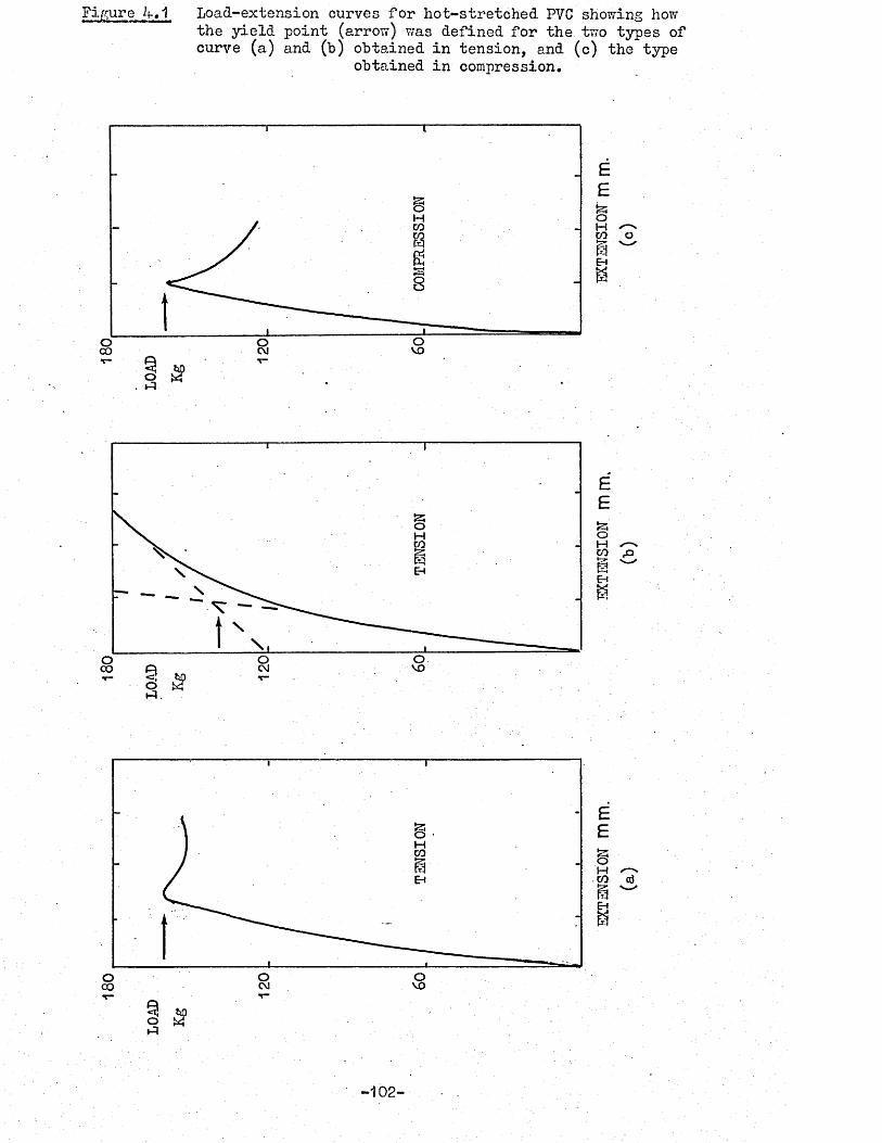
Figure if.j Load-extension curves for hot-stretched PVC showing how the yield point (arrow) was defined for the two types of curve (a) and (b) obtained in tension, and (c) the type

obtained in compression.

coEH

VOCOo

o

COo

EE£5oHCO0EHK-

oCO

oCO oCM ovo

E£oHco n}£1

o 3

-102-

Figure 4.2. Tensile yield stresses for ^ = 0° and 90°, plotted against draw ratio. A family of curves was obtained for drawing temperatures (T ) (70, 80, 90)°C.

200

NominalYieldStress

MNnf2

150

100

1 2 4-3 5Draw Ratio

-103-

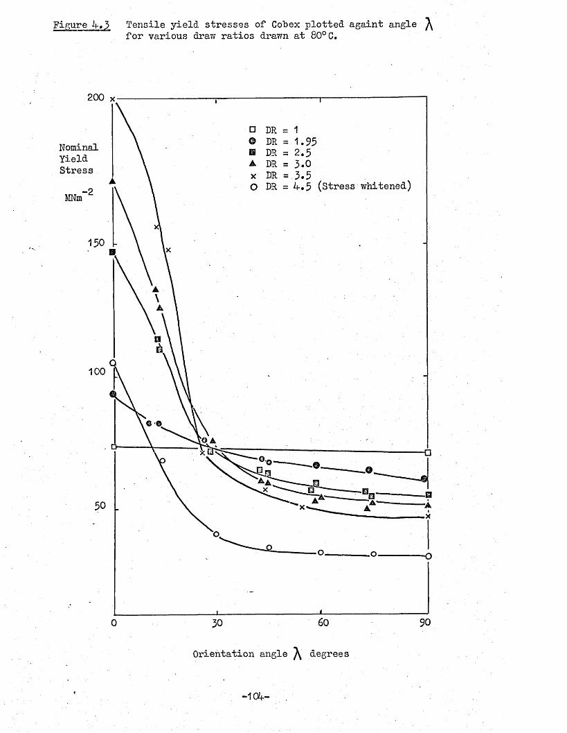
Figure 4.3 Tensile yield stresses of Cobex plotted againt angle ^for various draw ratios drawn at 80°C.

200 x

DR =.1.95 DR = 2.5 DR = 3.0 DR = 3.5DR■= 4.5 (Stress whitened)

NominalYieldStress

-2M m

150

100

60 900

Orientation angle ^ degrees

-104-

'igure k-tb- Nominal yield stresses plotted against draw ratio forvarious angles \ .

200

NominalYieldStress

150

100

1 2Draw Ratio

-105-

Figure A-»5a, Diagram illustrating the definitions of type 1 and type 2 deformation bands, and showing the sense in which and an( ^ are raeasure<3-*

Direction of type 2 band\

\\\

Sampletensileaxis

\

Figure U-.5b. Photograph shows # and bands illuminated by ’ polarised light and viewed with cross polarisers.

Direction of type 1 band//

Drawing

direction

(extinctiondirection)

-106-

Figure 4.6 Experimental values of Y plotted against ^ for various draw ratios. Material was Cobex drawn at 80°C>curves calculated by Hill theory using best fit determination of

ON

o x

VO

inco oN"V

in O inxx

crv

■5— O

o aP> cd

O

-107-

Orientation

Angle

Degree

Figure 4.7 Tensile and compression yield stress of Trovidur in the draw direction.

Onset of whitening

100

NominalYieldStress

Comoressionx

20

Draw Ratio

-108-

Figure 4.8 As-received PVC sheet: variation of tensile (x) and compressive (o) y .eld stress with temperature measured at a strain rate of 100^ min in the axis-1 direction, Tg and drawing temperaturesare indicated by a vertical solid and broken lines respectively,

X’TensionosCompression.• £ = 100^ min**

200YieldStress

150

100

40Temperature °C

Figure 4.9 Hot-stretched PVC sheet: variation of tensile (x) and compressive_j[o)' yield stress with temperature measured at a-strain rate of 100^ min in the hot-stretch direction. The vertical broken line indicates the hot-stretching temperature. The solid line indicatesTg (67°c)

X^Tension OsCompression k - I00?b min*"

200YieldStress

MNm

100

50

0Tg 800

Temperature °C

-105-\

Figure 4-.10 Hot-stretched PVC sheet: variation of tensile (x) and compressive^ (o) yield stress with temperature measured at a strain rate of l o min” in the hot-stretch direction. The vertical broken line indicates the hot-stretching temperature, Tg is indicated by the solid

verticalXs Tension o--compressio: £ = 1 fo min

200YieldStress

150M m

100

50

40Temperature °C

line i 67° C.

Figure 4,11 Measured compression yield stresses of Darvic plotted against angle ^ for various draw ratios.

100Yield I Stress X

M m

OR = 2.5 DR = 3.3

Orientation angle degrees

- 110-

Figure 4*12 Hot-stretched PVC sheet: variation of tensile and compression yield stress magnitudes with orientation angle ^ , the angle between the test-piece axis and the hot-stretch direction, measured at 20°C and a strain rate of 100j£ min : (X,o) experimental tensile and compressive yield stresses, respectively; (— -) tensile (t) and compressive (c) curves obtained from eq. (^5)with a single set of values for ay H, G-, and M*

cr\

o

H 0)<d h•H -P tO

03a>oUtiO0)

rHbQ

o•H-P-P£CD•HUO

-111-

Figure A-.13 Theoretical curves of tensile and compression yield stresses plotted against modified Hill criterion.

^ ; with Cq = 0, calculated from the

o\

o

<o

o

o

Xoo o

toto1-4 0> 0 k •H -P H CO

CMI6S

-112-

Orientation

Angle

A degrees-

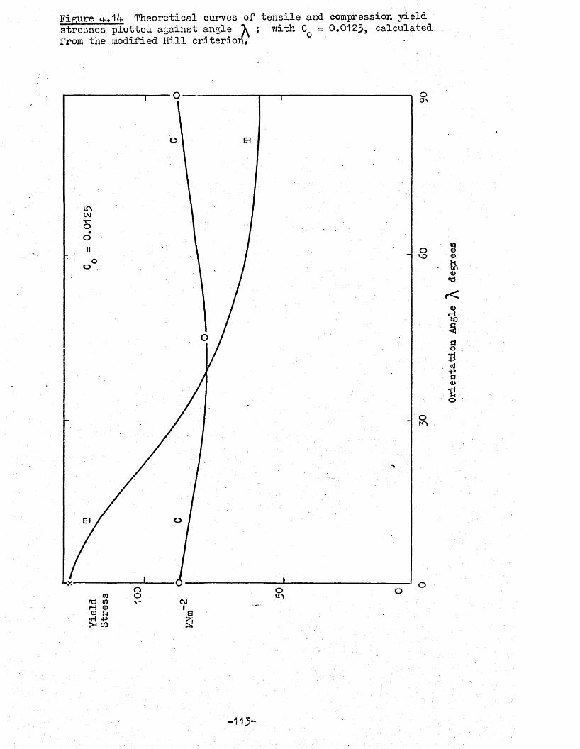
Yield

Stress

Figure ^.14 Theoretical curves of tensile and compression yield stresses plotted against angle ; with CQ = 0.0125, calculated from the modified Hill criterion.

a\

o

CM

o

o

V

-113-

Orientation

Angle

degrees

Figure 4.15 Experimental tensile yield stresses for Cobex plotted against angle ^ ; the curve has been calculated from the modified Hill criterion, a, was determined by band angle fitting. Drawing temperature was 70°C.

150

TrueTensileYieldStressMNnf2

100

\ o

50without a

060 900 30

Orientation Angle (degrees)

-114-

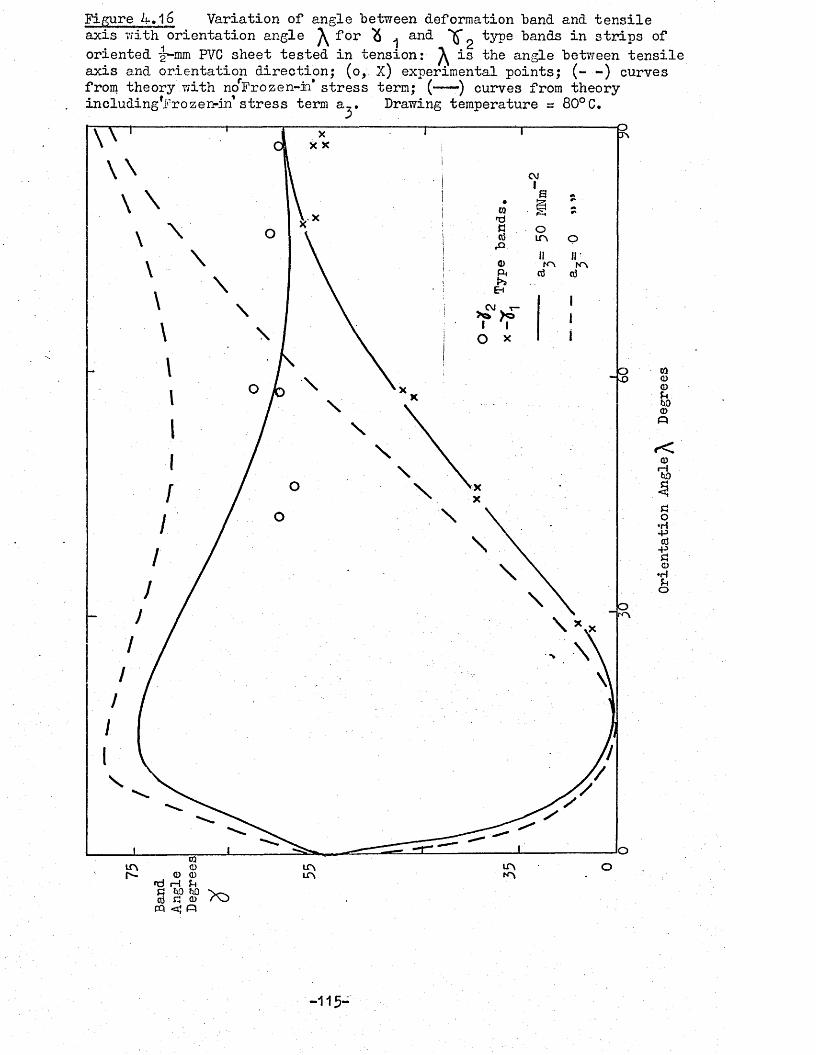
Figure 4.16 Variation of angle between deformation band and tensile axis with orientation angle ^ for "8 and type bands in strips oforiented -J-mm PVC sheet tested in tension: ^ is the angle between tensile axis and orientation direction; (o, X) experimental points; (- -) curvesfrom theory with no Frozen-in* stress term; (---) curves from theoryincluding^rozen-in* stress term a^. Drawing temperature = 80° C.

CM

in

inn

caooubOO<=»

CD r—1bD

o•H•P•P C5 CD •HUO

-115-

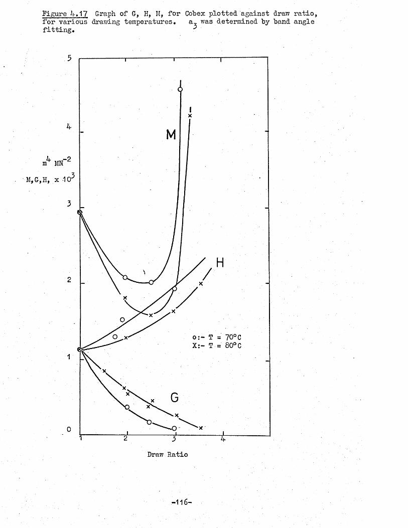
Figure 4.17 Graph of G, H, M, for Cobex plotted against draw ratio, for various drawing temperatures. a, was determined by band angle fitting.

5

,3M, G, H, x A Or

3

2

o:- T = 70°C X:- T = 80°C

1

0

Draw Ratio

-116-

Figure 4.18 Graph of frozen-in*stress, a, for Cobex plotted against draw ratio, for various drawing temperatures. a, was determined by band angle fitting C = 0. ^

80

M m " 2'Frozen-in*Stress COBEX

40

X-T = 70°C o-T = 80°C

0.1 2 3 4

Draw RatioFigure 4.19 Hot-stretched Darvic sheet: values of the 'Frozen-in’stress term a^ as a function of temperature measured at strain rates of100Jc min (A ) and 1 min ( □ )

40

A= 100^ min □ = 1 fc min

-2

10

Temperature °C

-117

Figure 4.20. Values of the ‘Frozen-in1 stress term, a, and maximum drawing stress as a function of draw ratio, for Cobex^rawn at 70°C

100 COBSXM m.Stress

O-Frozen-in stress x-Drawing stress

Draw Ratio

-118-

Figure 4 .21a. (S^)~2 plotted against mean yield stress.

3.0

(GNm -)

2.0

1.0

1202Mean Yield Stress M m

Figure 4,211), ( 33) 2 plotted against tensile yield stress

3.0

120Tensile Yield Stress MNnT2

-119-

Figure 4.22a (S^ “ ^ 3) 2 plotted against mean yield stress.

3.0

2.0

12040-2Mean Yield Stress MNm

1Figure 4.22b (S,^ - S^) 2 plotted against mean yield stress.

3.0

i32

402Tensile Yield Stress MNm

-120-

Figure 4*23* Load-extension curve obtained during the hot dravdng and cooling process* 0m, load maximum and Or, load minimum have been indicated*

200

150

LoadKg.

100

12Time Minutes

-121-

CHAPTER FITS

ULTRASONIC HLASTIC CONSTANTS

5.1 IntroductionIn chapter four the results from various tensile and

compression tests on bulk FTC were reported. The parameters, which described the anisotropy at yield, were derived by applying the modified Hill criterion. These parameters did not have any clearly defined relationship with any fundamental material constants. The experiments, .moreover, required a large number of samples of a particular material, and so consumed a large amount of material; the sample being either permanently deformed by plastic flow or fracture. The possible application of that form of test for routine quality control, especially for examination of small articles was limited by these experimental constraints. The tests did, nevertheless, provide useful information about the behaviour of oriented FTC that will be of use in design and fabrication technology where orientation could be accidently introduced.

• ■*An alternative approach to obtaining information about the

mechanical anisotropy of oriented FTC near yield was indicated by Hargreaves (8) who suggested that the tensile modulus of oriented polymers was simply related to the tensile yield stress; this being the case, the characterisation and prediction of the mechanical behaviour near yield could be simply undertaken by using a ‘non­destructive test method, that of’ measurement of the modulus of the polymer. The method chosen for this work was an ultrasonic method utilising the relationship between the elastic constants and the moduli of the material and the ultrasonic wave velocity in the

material. This method required only one small test sample.-122- ’ '

Also recent developments in the field of ultrasonic wave generators and transducers for transmitting and receiving of ultrasonic waves had started the present interest in the field of ultrasonics as a non-destructive test tool, in the general area of flaw and crack detection in metals and ceramics.

The elastic constants and moduli are fundamental properties of elastic materials, and so care had to he taken in the use of these constants in the description of the properties of viscoelastic polymers. It has been found, however, by Ward (47) and. Wright et al. (21) that for glassy polymers, such as rigid PVC, PS and FMMA, these were useful experimentally determinable constants.

In the present work, the experimental values of the velocities of propagation of the ultrasonic waves in the oriented PVC have been measured. The values were also used to calculate the elastic stiffness and compliance constants, which fully describe the anisotropy of the PVC. The experimental details and the theory of the method have been described in chapter three, together with the details of the calculation of the constants. This work has also been reported elsewhere (Rawson and Rider (44)).

5.2 Measured ultrasonic elastic constantsIn table and 5*2, the elastic stiffness and compliance

constants of the transversely isotropic PVC have been listed. The constants were calculated by applying the elastic wave theory derived by Musgrave (1) to the measured ultrasonic wave velocities propagating in various directions in the oriented PVC. ' The con­stants have been plotted in figures 5*3 and 5*4 as a function of birefringence and in figures 5*1 and 5*2 as a function of increasing draw ratio.

-123-

The change of ultrasonic elastic constants (C.y) with increasing orientation could be thus summarised as follows: C ^ (direction 3 was the draw direction and hence the preferred alignment direction of the molecules) rose v/ith increasing orient­ation, its value increased by about 95fc: j , however, showed littleor no change, at most a fall of 10%: C^, all rose initially,

and then dropped slightly and remained level. The maximum changes were about 13% for C^, 60% for and 70% for

The experimental uncertainties of these values as mentioned in chapter three were about £ 1,3/° in the constant and 3*7% in the other constants; the differences between the elastic constants measured on samples nominally similar was about 3*0%, which was within the estimated uncertainties of the experimental measurements.

The compliance constants (S^) in general had a greater uncertainty because each was calculated using a combination of the Ch *s. The uncertainties were consequently as much as 10%, except for S; j , which was simply the reciprocal of CA V The over­all change in compliance constants has been plotted in figures 5*2 and 5*4: decreased by about 30%: showed no significantchange, a possible small rise of 11%: S^, fell initially and then rose to a maximum at a draw ratio.of 2.5, decreasing vrith further increases in draw ratios. Maximum change of S12 was about 110^, and was 30%: showed a small total decrease of 20%after an initial rise.

5.3 DiscussionThe values of the ultrasonic elastic constants of oriented FVC

reported in section 5*2 were measured, using a transmitter technique developed at the National Physical Laboratories by Markham (20).

-124-

Wight, vftiite, Faraday and Treloar (21) have also reported measure­ments of the ultrasonic elastic contents of two other oriented polymers, PS and H.IMA. They developed a technique involving the reflection of the ultrasonic waves at the liquid/polymer surface.They determined the critical angle for the transverse and longitu­dinal waves, by monitoring the reflected beam intensity which changed characteristically at the critical angle. From the critical angle data, the wave velocity in the material was determined, and by using Musgrave’s analysis of the theory of wave propagation in anisotropic media, the elastic constants were calculated. It was outside the scope of this work to directly compare the two techniques, which Y/ould involve repeating measurements on the same samples on the two pieces of equipment, preferably by the same operator. The relative merits of the methods could then be examined in detail; it would appear, however, that the errors in the two methods were comparable about £ 3*7/o for most of the constants.

The materials tested by bright et al. (21) were PS and BSIA oriented by extension to a fixed draw ratio, using different drawing temperatures. Their results for PS showed no change in the constants, and less than 10^ increase for C^,and a similar decrease for over the range of orientations tested (Birefringence A n = 0 — 14 x 10*” ). The EMMA results showed larger monotonic changes with increasing orientation (Birefringence range 0 — - 16 x 10~^). The elastic constant increased by 35%; the and constants increased by less than 3%i the and decreased by less than 10%.These changes were much the same as those of the PVC; however, the degree of orientation of the three polymers could be quite different. Since values for the maximum birefringence of PVC and PMMA have been reported in the literature, and using the

-125-

concept of a fully oriented polymer having the net birefringenceof a single molecular unit, a normalised birefringence max)could be used as the abscissa in replotting the elastic constants,as a function of orientation. The experimental variation of drawratio and birefringence has been plotted in figure 3*6 and figure

(c =Sfl,W w ).' shows the data plotted in'this form^ The value ofAn max

for RJMA used was 4.3 x 10 (Kashiwagi, 26) and for PVC-A n max = 5.5 x 10 3. This value was obtained from the TTardtheory calculations table 3.4. The PVC drawn to draw ratio of3 (Figure 5*'0 could thus be seen to be much more highly orientedthan, the EMMA used by vTright et al., on this basis of- comparison.The increase in the C,7 constants of PVC and BSMA at^n/ h33 / A n max= 0,36 T/ere now about 130/£ and 140^, respectively. It was thus seen that the elastic constants of FMMA and PVC behaved in a similar manner with increasing orientation over the range available for comparison, A value of A n ^or PS was not available and soUlclXthe PS could not be replotted in this form.

The measured values of the elastic constants have been seen to vary with increasing orientation; a simple model was considered to explain the observed variations. The oriented PVC was envisaged with the molecules partially extended as planar zig-zag chains.This could then be analogous to a ,two-phase material, one phase, the extended molecules, and the other, the random molecules. An aggregate two-phase model originally proposed by Kuhn and Grtln (9) and, more- recently, successfully applied by Yfard (47) and Gupta and Ward (46) to polyethylene was then used to analyse the oriented PVC results. Kashiwagi et al. (26) have also applied this model to the results of bright et al. (21) on RIMA and P3.

-126-

The model assumed a two-phase material, a non-active matrix containing transversely isotropic units, having five independent

elastic constants = C11U’ c12 > C33U’ V and five.associated compliance constants S. .U. The units could be related to the extended molecular chains, and the non-active matrix the random coiled molecules; these considerations were not, however, discussed . in detail at this stage. It was assumed that in the isotropic polymer, the units had a random distribution of orient­ation. As the sample was oriented, the deformation caused theunits to rotate and become aligned. The polymer observed elastic

uconstants were obtained- by averaging the unit constants orC. ,u. Two methods of averaging were used, that of averaging the 10stiffness constants C. .u (Voigt average) and the second was3-0determined by averaging.the compliance constants S..U (Reuss average) and the corresponding stiffness constants were then calcu­lated, using the relationship between C^'s and ft-7).also assigned each unit a value of birefringence of An , and • • . max’hence by averaging the contributions of each unit, the material birefringence could be calculated. Ward*s expression for the averaged constants could be written:-

S. . = S. .U + A?, .x Sin^ 0 + B a. Sin2 8 ... 5.1•3-0 3.J (3-0) (3.0)

C. . = C. .U + aT. Sin^ 0 + bT. Sin2 0 ... 5.23.J ij (3-0) (3-o)

A n = An (1 “ o sin2 ® ) ••• 5*3max x 2 7R R v vwhere A ^ . y B^j-; an< ^(ij) are *unc^ ons °**

S..U and C..U in table 5*5*3-0 3-0

0 is the angle between the symmetry axis of the unit and the draw direction (3).

-127-

. 4 2Sin © and Sin © were explicit expressions in terms of the draw ratio derived by v/ard (47) on the assumptions that individual unit rotated affinaly without change in properties, that the drawing strain was transversely isotropic and that no change in volume occurred during drawing. The numerical values of these expressions evaluated by Ward (47) were used in' determining the material constants and unit constants. In table 5*6 the values of the expressions obtained by Ward have been listed.

The unit elastic constants were determined by fitting the theoretical expressions for the Voigt and Reuss averages of elastic constants and the birefringence at one particular draw ratio; not at unity where only three independent constants exist. The theoretical expressions were then used to calculate the birefringence and elastic constants at other draw ratios, including unity for comparison with the experimental values,

The curves plotted in figures 5*9 and 5*6 were theoreticalcurves fitted at a draw ratio of 3*3* the curves for the stiffnessconstant being obtained from equation 5*1, (the Reuss average).The unit values of S^, and the corresponding values of andA n have been tabulated in table 5*4 Voigt average,maxequation 5*2, gave the curves plotted in figures 5*7 and 3*8.The 'fitting points were draw ratios of 3*3 and 1.45 respectively.In each of the graphs 5*6 to 5*9, the lines indicate theoretical calculations and the plotting symbols indicate experimentally measured values.

It can be seen from the graphs 5*7> 3*8, •5*9* that the' Voigt average gave a distinctly worse agreement of theory and experiment

-128-

than the Reuss average. The Voigt average fitted at DR 3*3 was, however, considerably better than the curves fitted to DR 1.45*The improvement of the Reuss average over the Voigt average can be clearly seen in the agreement at low draw ratios. The theory does not, however, accurately describe the undrawn values of the elastic constant. The C,, = C,, values were 15% and the C„0 = C.,11 33 12 13values .were k-5% over estimated by the model. Apart from theundrawn case the experiment and theory were within 10% and inmany cases within 5/*

The theoretical case for the An was bound to fit not only atthe fitting point (DR = 3*3) but also at draw ratio of unity,since it was independent of the value of A n • Figure 3*6 * ■ max .shows that the theory also over-estimated the experimental valuesover the lower range of draw ratios. The value of^n = 5*5 x 10 ^. max

- Vwas not very different from the value of 7*2 x 10- found by Rider and. Hargreaves (7) for another type of PVC Vybak PVR 294 (Bakelite Ltd.) drawn at room temperature.

Considering the simple nature of the model from which other results were calculated, the theoretical values 7/ere in quite good agreement with the experimental ones•

For the undrawn PVC, the model over-estimated the values of the constants; a reason for this could be the initial assumption that the units moved by affine rotation was not valid at low draw ratios. For the transition from coiled to particularly extended configuration, it could be thought that the number of segments contributing increased; there being no segments contri­buting when randomly coiled and they only contributed when partially extended. As the'draw ratio increased, the percentage of created

129-

units would then rapidly fall, and the affine rotation process

would then predominate. The effect of temperature on the efficiency of drawing to align the molecules "by this model would "be assumed to "be constant. However, as the drawing temperature was increased, the molecular alignment was less for a given draw ratio, as was seen in the birefringence change with draw ratio, graph; figure 3*13* Also this effect can be seen in the yield stresses at 0? showing the values at the same draw ratio, and various drawing temperatures, figure 4.2. This process of chain slippage was possible because of the lack of chemical crosslinks. The thermal crosslinks of entanglements were reduced with increasing temperature as the molecules became more mobile.The fit of the theory would thus presumably become worse as chain slippage increased; any stress induced crystallization occurring would give an effect masking the slipping process. No measure­ments of elastic constants were available for this material drawn at higher temperatures to check these suggestions.

Kashiwagi et al. (26) have applied V/ard*s model to the PMMAresults of -i/right et al. (21), discussed earlier. The differingdegrees of orientation in the RIMA were produced by drawing to thesame extension at different temperatures. It was therefore not

4 ' 2possible to obtain values of Sin 0 and Sin 0 from the draw ratio.Kashiwagi et al. obtained these values from measurements of theproton-magnetic resonance second moment. They were then able tofind a value for A n from equation 5,3• They extrapolatedmaxlinearly from the measured values of the elastic*constants to thebirefringence value equal to^n , and took the extrapolated valuesmaxas the elastic constants of the unit C. .U. They were then able toij Jcalculate the Voigt and Reuss averages of the elastic constants for

-13C-

the whole range of orientations from the theory, and they found that the measured values lay between the two, as would be expected from the theory.

The aggregate model had thus been able to predict the general variation of the ultrasonic elastic constants of three polymers.The intention which led to the determination of the ultrasonic elastic constants was to examine the relationship of the yield stress with the ultrasonic modulus. The calculation of the modulus and the discussion of such a relationship has been made in chapter six.

-131-

TABLE 5.1 PAR.VIC 5.5 mm SHEET. DRAW AT 80°CElastic stiffness constants C.

measured ultrasonically.+ -5Density P = 1390-1kgm

-2Stiffness Constants in G-Nm Draw Ratio Birefringence x 10^ C^ ^12 ^13 ^33 ^44

1.00 0.11 6.30 2.77 .2.77 6.30 1.80 1.43 0.78 7.26 3.50 3.90 7.62 1.601.75 1.60 7.16 4.16 4.34 9.12 1.682.15 2.01 7.18 4.07 4.79 9.59 1.742.50 2.67 6.95 4.50 4.3 9.75 1.652.70 3.27 6.86 4.46 4.47 10.50 1.753.00 3.45 6.65 3.88 4.43 11.70 1.393.30 3.63 6.68 3.74 4.79 11.85 1.58

TABLE 5.2DARVIC 5.5 mm SHEET, DRAwN AT 80°CConroliance constants S. . calculatedi Jfrom the ultrasonically measured stiffnessconstants C..■ iJ.

N 2 —1Compliance Constants in m (ON)

Draw Ratio Birefringence x 10^ 11 ^12 ^13 ^33 **441.00 0.11 0.217 -0.066 -0.066 0.217 0.5551.45 0.78 0.207 -0.059

VOr-o•01 0.209 0.6251.75 1.60 0.276 -0.097 -0.068 0.173 0.5952.50 2.67 0.269 -0.138 -0.058 0.149 0.6062.70 3.27 0.275 -0.142 -0.057 0.143 0.5713.00 - 3.45 - 0.250 -0.111 -0.053 0.125 0.7193.30 . 3.63 0.246 -0.094 -0.062 0.134 0.633

r132-

TABLE 5.3

Values of C..U used to fit experimentalZL Jdata, for a draw ratio of :1;»45 & 3*3»

Voigt average

ij 11 12 13 33 44 DR

C. .u GHm-2 7.9 2.7 3.3 10.6 0.2 3.33-J

C. .u " 6.2 3.4 4.7 14.0 1.3 1.453-0

TABLE 5.4

Values of C ^ , and A n max used tofit the experimental data at a draw ratio

of 3*3 B.euss average.

ij 11 12 13 33 44

S. .u m2(GH)"1 0.25 -0.10 -0.044 0.072 0.663-0

C± u W 2 6.6 3.8 6.3 21.6 1.47

= 5.5 x 10-3max

-133-

EXPRESSIONS FOR AND COEFFICIENTS

FOR EQUATION (5.2)

c ■ a* bT...'ij (ij) (ij)

C11a- r u 8 Co

C121 n U 8 0

C13 -i C u * 0

C33 c u0

C44 -4 c u 0where C u = Cj . u

u u u13 + 44 “ 11

C13u r u12, U p u'11 + 12 ". U r* U13 ” 33 +

- C12U - 4C13U +2C33U-10V U)

EXPRESSIONS F (H A ( i j ) ARDB( i j ) IN EQUATION (5 .1 )

S. . .R _RIJ ( i j ) ( i j )

S113 Q u8 So S13 + ^ S44 - s u

11

CMv-CO 1 o u

8 Soq «'■ _ O U .

13 12

S13- f s u * 0

± (o * . q U 2 iS1 t + S12 - 3 S13U + S' U - ‘33

S33r. USo 2 (^ 1 3 U “ S33U 2 44 }

3CO - 2 S u 0 3 S 11U - S i 2U - 4 S13U + 2 s u - 33

. £q U2^44

where <5 u _ c USo ~ 11 + S33U “ 2 S13* ~ S fU

-134-

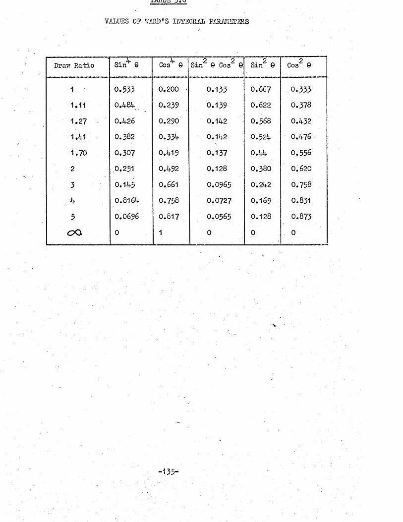
VALUES OF YARD'S INTEGRAL PARAMETERS

Draw Ratio ' IT--------Sin 9 ~ 4 Cos 9 Sin2 9 Cos2 9 Sin2 9 Cos2 9

1 0.533 0 .200 0 .133 0.667 0 .333

1.11 0 .484 0 .239 0.139 0.622 0.378

1 .27 0 .426 0.290 0.142 0.568 0.432

1.41 0.382 0.334 0.142 0.524 0 .476

1 .70 0 .307 0.419 0 .137 0 .4 4 0 .556

2 0.251 0.492 0.128 0.380 0.6203 0.145 0.661 0.0965 0.242 0.758

4 0.8164 0.758 0.0727 0.169 0.831

5 0.0696 0.817 0.0565 0.128 0.873

O Q 0 1 0 0 0

-135-

Figure 5.1 Plot of the experimentally measured ultrasonic elastic constants (C..) of oriented PVC against draw ratioIJ

a-0

GNm

12

8-2

4 -o

0

Draw RatioFigure 5*2 Plot of the experimentally measured ultrasonic elastic compliances (S..) of oriented PVC against draw ratio.

0.7

0.5

0.25

0.15

0.0,

Draw Ratio

-136-

meaaux-tju values or u. . p-Lovcea against; Dirernngence.

12

■2G-Nm

O O-

3Birefringence x 10

Figure 5*4 Measured values of S. . plotted against birefringence.

0.700.50

Q.20m GN

0.10

Birefringence x 10'

-137-

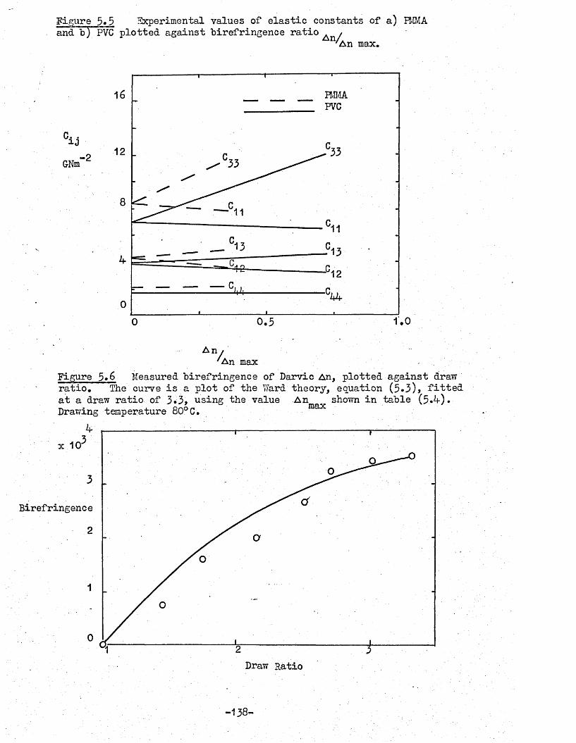
Figure 5.5 Experimental values of elastic constants of a) FMMA and b) PVC plotted against birefringence ratio . /

'An max.

cuG-Nm-2

16 FMMAPVC

12

8

4

01.00.50

An /'An max

Figure 5.6 Measured birefringence of Darvic An, plotted against draw ratio. The curve is a plot of the T/ard theory, equation (5*3)> fitted at a draw ratio of 3*3, using the value A n mov shown in table (5*4). Drawing temperature 80°C. max

4x 10-

3 .

Birefringence2

Draw Ratio

-138-

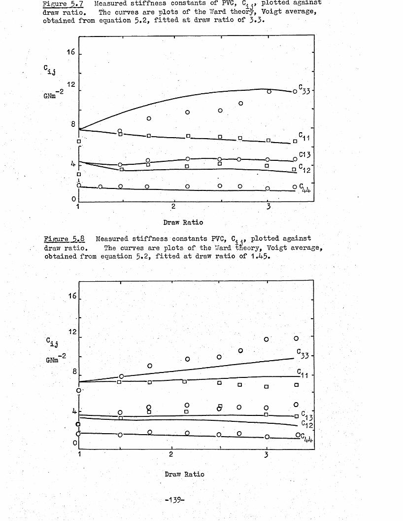
Figure 5.7 Measured stiffness constants of PVC, C.., plotted against draw ratio* The curves are plots of the Ward theory, Voigt average, obtained from equation 5.2, fitted at draw ratio of 3*3-

C. .iO

GNm-2

16

12

8

C134

0

Draw Ratio48 Measured stiffness constants FVC, C. plotted against

draw ratio. The curves are plots of the Ward theory, Voigt average, obtained from equation 5*2, fitted at draw ratio of 1.45.

12

GNm

1 2

Draw Ratio

-139-

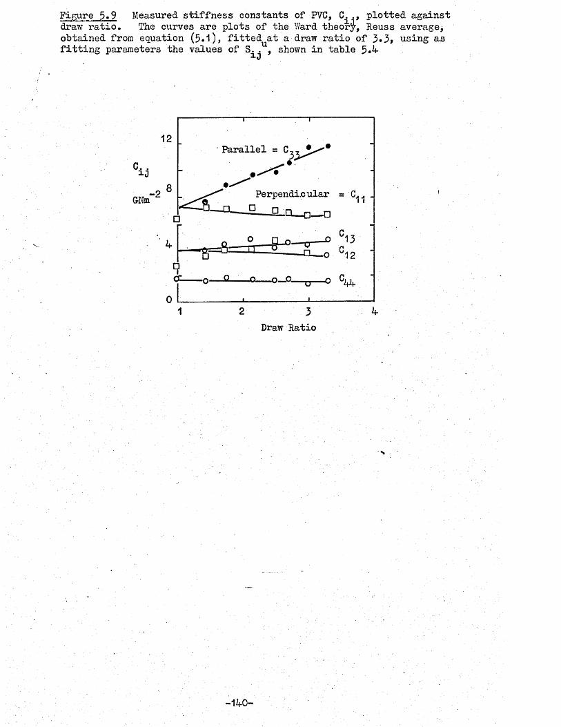
Figure 5 .9 Measured stiffness constants of PVC, C.plotted against draw ratio. The curves are plots of the Ward theor -, Reuss average, obtained from equation (5.1), fitted at a draw ratio of 3*3, using as fitting parameters the values of S. . , shown in table 5*4-

12• Parallel =

8 Perpendi.c ular 11 -

i— a

031 2

Draw Ratio

-140-

CHAPTER SIX

A CORRELATION BETWEEN YOUNG-*S MODULUS WITH YIELD STRESS IN ORIENTED POLYVINYL CHLORIDE

6.1 Introduction

Hargreaves (8), Robertson (28), Vincent (11) Allison and Ward (34), Bridle et al. (22) suggested that there was a correlation between the change in tensile yield stress and Young*s modulus which occurred when some thermoplastic was oriented. The existence of such a correlation will be discussed for oriented PVC.

Elastic constants and yield stress data for oriented PVC was reported in earlier chapters. The ultrasonic modulus was.obtained from the elastic constants, using the relationship given in section 6.3* In the present work, consideration has been given not only to the tensile yield stress, but also to the compression yield stress. The modulus was obtained from measurements at 5 'MHz'by an ultrasonic method, rather than from the load extension curve. However, some results obtained from the load-extension curve have been used for the sake of completeness, but the significance of these results was reduced by the errors involved in their determ­ination. This work has been discussed elsewhere (Rawson and Rider (39)).

6.2 Strain from load-extension curvesIn chapter four, the yield stress was discussed; the stress

was applied by straining the sample, resulting in an applied stress so both strain and stress should be considered when physical pro­perties are measured. Strains in the small samples of PVC were more difficult to measure accurately than the stress, because the small size of the sample prevented the attachment of strain gauges

-141-

or transducers. The various techniques used to measure the strain were given in chapter three.

The manufacturers* data for Darvic gave the strain to yield as 3 - 4/2. For Cobex the tensile strain to yield was given as k-%.

The strain to yield determined by the photographic technique gave an overall strain yield for oriented FVC (DR = 2.0, 2.7> 3*3) for both tensile and compression tests to be between 4 and Qfo (Figure 6.1a & b). The isotropic value for the compression yield strain by this technique was 6%, Because of the intervals at which photographs were obtained (1$ strain intervals), each measure­ment gave up to - ^% error. Other errors occurring as a result of extracting the data from the load extension curves, and from gauge length changes because of slipping from the grips amounted to about another £ to 1 An extensometer was able to be used on a few tensile samples of isotropic Darvic which had increased gauge length. This method gave a strain to yield of 4*1 - 0.1 2 .

A possible angular dependence of.strain was detected, indicating that the tensile strain at 45° was a minimum, and the compression strain was a maximum, figures 6.1a & b; the degree of orientation did not show any appreciable change in strain values.

Values of strain to yield taken directly from the load exten­sion curves, however, gave a mean tensile strain to yield of 6 - 2/2

|and the compression strain of 8 - 2.5/4 values greater than recorded by the photographic technique. The addition errors due to machine/ chart couplings, unknown gauge lengths, etc., meant that these values could only be used as an indication of the magnitude of the strain. Both values were higher than those determined from the photographs and unexpectedly the compression value was greater than

-142-

the tensile value. Since the compression test results give no gauge length or grip slipping errors, the compression strain might have been expected to be near to the photographic values.The machine coupling error at low speeds could of course account for this discrepancy.

To resolve further the strain variations with degree of orientation and angle of orientation in the sample, a micro form of extensometer could be developed. A direct reading optical non-contact test method v/ould be the most easily used system for use on this form of miniature sample held between anvils, which prohibit use of existing mechanical extensometers.

Because of the errors involved in the strain measurements off the load-extension curves the modulus values calculated from the curves have not been fully quoted. Some modulus ratio values have been used in section 6.4 since systematic errors due to the tenso- meter etc should have been eliminated. s

6.3 Ultrasonic modulusYoungfs modulus can be expressed in terms of the five

compliance constants for a transversely isotropic elastic^ material (Nye (43)), equation 6.1)

_l_ = S ^ S i n ^ t S33Cos^^+ (S^ + 2 S., ) Sin2 Xcos2 A ... 6.1E Xwhere E^was the

Using this expression, the modulus variation for the oriented FVC was calculated. Figure 6.2 ..showed the calculated ultrasonic modulus for several draw ratios. The general variation of the modulus was seen to be similar to that of the tensile yield stress, see chapter four (figure 4*3)* Figure 6.3 showed the change of modulus with increasing birefringence for y\= 0° and 90°• These

. -143- ■

Young*s modulus at an angle Xto the draw ratio.

-5values refer to measurements made at a strain of 10 (0.001^) anda frequency of 5 MKz* The strains of the moduli obtained from the

—2tensometer load-extension curves were of the order of 10 .(1.0$) •Thomas, Fleet, Meyer and Abraham (12) reported measurements of ultrasonic moduli and tensile *static! moduli of PP. The static moduli were measured at a strain of 0.1 and 1.0fo. They showedthat the extrapolation of the tensile moduli to very small strains gave up to 200fo increase in the modulus value, approximately that of their ultrasonic values. They suggested that the ultrasonic and static moduli would differ because of an effective temperature shift of the measurements caused by the frequency changes. They concluded that quantitative prediction of large strain moduli from the ultrasonic-moduli could not be made in detail, because of viscoelastic considerations. Other authors have reported similar changes in moduli. Wright et al. (21), in their measurements on FMMA, found about a 100?$ increase for the ultrasonic measured values over the *static* ones. The general increase in 2^ -®oq>both cases were similar. Reynolds (23,24) reported ultrasonic and static moduli of carbon fibre composites (50?c loading of fibre).He found the magnitude of the moduli by the two methods to be the

10 -? in vsame - 2 x 10 lift at J\= 0°; and 1 x 10 Nm 90°, thusdemonstrating the self-consistency of the method for non-time- dependent materials. The shapes of the curves showed some distinct differences. The static curve was concave in shape; his ultrasonic curve was convex. So that 45°, a 50/o variation was measured.

6*^ Correlation between Young*s modulus and yield stressIn the previous section, the Young*s modulus variation with

increasing orientation and orientation angle 7/as discussed. A similarity between ultrasonic, moduli and the tensile yield stress

; . . -144-

was observed (figures 4.3 and 6.2). The extent to which any correlation existed will be discussed in this section.

To use all available data on oriented PVC, a normalising .procedure was adopted, namely, by using birefringence as a measure 'of orientation, and by dividing the yield stresses and moduli by the value obtained for the appropriate grade of unoriented PVC, giving a quantity referred to as the yield stress ratio, or modulus ratio.Data for Cob ex, Darvic and Vybak (Vybak measurements were made by E. Hargreaves on PVC, similar to Cobex, made by BXL) have been presented in this form in figures 6.4 - 6.11'.

The similarity of the ultrasonic modulus ratio and the tensileyield stress ratio curves was quite distinct. No such similarityexists between the ultrasonic modulus ratio and compression yield

•47stress ratio curves, figures 6.4^and 6.8^>6 Only one set of data was obtained by the ultrasonic method, that being some average of tensile and compression mode of vibration, either side of zero strain.

The close similarity in behaviour between Young’s modulus and tensile yield stress could be clearly seen in figure 6.10 in which the tensile yield stress ratio was plotted against the modulus ratio, using the smoothed values read from the curves in figures 6.4 and 6.5, for ^ = 0° and 90°, for the same set of birefringencevalues and from the curves in figures 6.8 and 6.9 for intermediate

*v + -3 ■values of. /\ for a birefringence of 3*6 - 1 x 10 J. All thepoints lay close to a common straight line. Similarly, in figure 6.11 the results for the static measurements have been plotted using data from the load extension curves. Both the tensile and compression points could be represented by straight lines. The large scatter was probably due to the larger errors in the static

moduli

These experimental results could be written:

E0.85 I X I -2.45 ... 6.2

Eu us

1.40 f EX —0*4- • • • 6*3

“3.2 f X V +2.2f5 ... 6.4-

where CT , (f and Ev were the yield stress, of the oriented A u APVC at angle ^ ; the yield stress of the as-received FVC and the Young’s modulus at angle , respectively* The subscripts us; t; and c; indicated the ultrasonic, tensile and compression equations*

Thus a close correlation between the ultrasonic Young’s* Nmodulus ratio and yield stress ratios could be seen* In addition, the static moduli showed a similar correlation for both the tensile and compression measurements* Since an equation of the same f o m could be found for each of these three cases; this may form the basis of a method of determining the tensile yield stress of oriented FVC (and perhaps other thermoplastics) from the ultrasonic elastic constant measurements, which could be advantageous in some circumstances* The precautions required to ensure accurate results because of the variations outlined above could cause many difficulties*

-146-

Figure 6.1a. Measured values of tensile strain at yield for variousdraw ratios plotted against angle ^ , calculated from photographs.

StrainTension

Orientation Angle ^ DegreesFigure 6.1b Measured values of compression strain at yield for various draw ratios plotted against , calculated from photographs.

8

Strain

Compression

DR = 2.7 DR = 2 DR = 1

Orientation Angle Degrees

Figure 6.2 Measured ultrasonic small strain Young*s modulusplotted against angle \ •

DR = 3.3 DR = 2.7 DR = 1.93 DR = 1.0

Young*s Modulus

GfrmA

Orientation Angle Degrees

Figure 6.3 Measured ultrasonic small strain Young*s modulus plotted against birefringence.

Young*s Modulus

2G-Nm

,3Birefringence /x 10'

-148-

Figure 6.4- Variation with degree of orientation, indicated by birefringence, of the ratio of the ultrasonically determined Young’s modulus of orientated PVC to that of the unoriented material, for directions parallel to 0° (□ ), and at right angles to V= 90° (■'), the orientation direction. The material was Darvic oriented by drawing at 80°C to the residual birefringence shown.

Young’sModulusRatio

1 2 , 3 4Birefringence x 10

Figure 6.5 -Variation with degree of orientation, indicated by birefringence, of the ratio of the tensile yield stress of oriented PVC to that of the unoriented material, for directions parallel to,*(A = °°) and at right-angles to,( 90°), the orientation direction. The materials, orienting draw temperature and direction are indicated as follows:

“ ' -2.5TensileYieldStressRatio

1.5

Material . Draw Temperature

(°c)Symbol

A= o° A= 90°Darvic 80 □ HCobex 80 O . •Vybak 71 V ▼Vybak 90 A A

0.5ice x 10

Figure 6.6 Variation v/ith direction of the ratio of the compressive yield stress of oriented PVC to that of the unoriented material. This example is Darvic oriented by drawing at 80°C to a residual birefring­ence of 3*63 x 10

2.0Compressive Yield Stress Ratio

Orientation -Angle Degrees

Figure 6.7 Variation vdth degree of orientation, indicated by birefringence, of the ratio of the compressive yield stress of oriented PVC to that of the unoriented material, for directions parallel to \ = 0° ".(□), and at right angles to \ = 90° (■), the orientation.'direction. The material was Darvic oriented by drawing at 80°C to the residual birefringence shown.

2.5,

CompressiveYieldStressRatio

■0.50 1 if2

Birefringence x 10'3

-150-

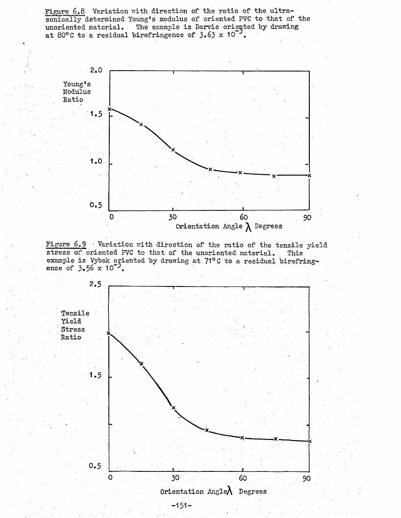
Figure 6.8 Variation with direction of the ratio of the ultra- sonically determined Young's modulus of oriented PVC to that of the unoriented material. The example is Darvic oriented by drawing at 80°C to a residual birefringence of 3.63 x 10 .

2.0Young'sModulusRatio

1.0

0.5600 30 90

Orientation Angle Degrees

Figure 6.9 ’ Variation with direction of the ratio of the tensile yieldstress of oriented PVC to that of the unoriented material. This example is Vybak oriented by drawing at 71 °C to a residual birefring-onf>o n-P ^ -v ACT**

2.5

TensileYieldStressRatio

1.5

0.5

Orientation AngleA Degrees -151-

Figure 6.10 Tensile yield stress ratio plotted against ultrasonicallydetermined Young’s modulus ratio. Source of date: for a range ofdirections, birefringence 3.6 x 10 , Figures 6.8 and 6.3; O, for arange of birefringence, parallel to the orientation direction, upper curves of Figures 6.k- and 6.5; • , for a range of birefringence, atright-angles to the orientation direction, lower curves of Figures 6.k- and 6.5.

o

co

o

CM

-152-

Figure 6.11 Large strain tensile and compression yield stress ratioplotted against Youngls modulus ratio.

co

o o COoo

CMCO0 8CO P8

■153:

CHAPTER SEVEN

FRACTURE-OF ORIENTED POLYVINYL CHLORIDE

7*1 Introduction

The fracture of oriented PVC was not the primary interest of this investigation; however, the failure hy fracture rather than hy yielding of some samples at room temperature was observed. Fracture of the thick sheet oriented tensile samples was the predominant failure process. . So, some investigation of the brittle-ductile transition in oriented PVC was made insofar as it affected the yielding behaviour. To complement the tensile tests and obtain fracture in samples cut at all angles of orientation, Charpy impact tests were made on the oriented PVC,

The ductile-brittle transition in isotropic polymers is a well known phenomenon and has been extensively examined by Vincent (11,33) and Andrews (37)# As the transition temperature is strain rate dependent for a tensile test (time scale of 1 sec,), the brittle temperature is about -80° C (Vincent 3), and for a notched impact test IS (4) (time scale of 10"^ sec.) it is about 20°C. The transition is also dependent on the notch radius.

7.2 Tensile fractureBoth the thin Cobex sheet and the thick Darvic sheet in the

as-received or isotropic state yielded when tested in tension at room temperature. The thick isotropic Darvic sheet was also tested in tension at temperatures as low as -60° C and all the samples tested yielded. The oriented PVC sheet, however, exhibited some tensile fracture behaviour. The thick sheet samples showed the greater tendency to fracture.

-13+-

For thin sheet oriented samples with the orientation direction at ]\=90° to the tensile axis, fracture was observed along the orientation direction, for samples drawn at 80°C with draw ratio greater than 3*5* Stress whitened samples of draw ratio 3.7 and greater, yielded. Samples drawn at 9.0° C fractured for orientations greater than 2.5, figure 7*1*

For samples tested with the orientation direction at ^ = 0°, drawn at 80°C, fracture occurred if the draw ratio exceeded 2.3.The samples fractured w'ith the surface perpendicular to the tensile axis and the chain alignment direction, near the one side of the sample, a step in the fracture surface was observed, see figure 7*2. The stress whitened samples also failed in the same manner with yielding. Sheet oriented at 90°C tested at ^ = 0° had a tendency to split with cracks propagating along the molecular alignment direction for draw ratios up to 3*0; for larger draw ratios, the samples split into several sections and gave a fibrous fracture surface, figure 7*3* ^he orientation as measured by birefringence (see chapter A) was less than samples drawn at 80° C with a' draw ratio of 2.3. These longitudinal cracks were sometimes observed

fbin samples which had been drawn at 90°Cj high draw ratios. N The stress whitening did not occur for samples drawn at 90°C. Samples tested at angles other than \ - 0° and 90° and drawn at 80° C and 90°C yielded when tested in tension.

Thick oriented Darvic sheet samples, drawn at 80°C, showed a greater tendency to fracture. The samples tested for ^=90° all fractured except for draw ratio 1.7* For draw ratios greater than 1.7 only the samples with orientation at angles of ^ less than30° yielded and for draw ratio greater than 2.5 all the samples fractured. The fracture surface was smooth and parallel to the

-155-

molecular alignment direction. Samples fracturing at ^ = 0° were fibrous and tough. Figure 7*4 shows the yield fracture transition. Samples with draw ratio of 2.6 were tested at tempera­tures of 20, 30, 40, 50, 60°C. The yield fracture transition moved to higher angles and all the samples yielded when tested at 50° C; the degree of orientation of the samples was probably affected at that temperature. Samples cut with 0° with various geometries were tested at 20° C to see if the fracture failure could be suppressed, but all the samples fractured.

7.2.1. DiscussionThe observed features of the tensile fracture of oriented PVC

samples with ^ = 9 0 ° would be consistent with the ideas of .Vincent (3, 11, 33) shown schematically in figure 7«5- The graph shows the change of yield stress and fracture stress of anisotropic polymer with temperature near the transition temperature. The failure mechanism that Operated at a given temperature was that which required the lower stress. The oriented polymer has aligned molecules such that the number of strong carbon-carbon bonds of the molecular back­bone per-unit area increase in the axial direction and hence leaves a decreased number of bonds per unit area in the transverse direction. The fracture process which involves creating new surface area consequently requires less energy to operate for }\= 90° as the orientation increases; but the fracture stress in the orientation direction = 0° increases rapidly as the number of back bone carbon-carbon bonds which had to be broken increased. The yield process involves molecular rearrangement in a given volume and so depends on movements in all directions. In the transverse direction, the anisotropy was not so marked.

-156-

So the sample of oriented PVC could fracture at ^ =90°.The transition back to yielding of the stress whitened PVC could be due to the increased microvoid content allowing the molecules greater freedom of movement and thus lower the yield stress below the fracture stress. Hargreaves had suggested that the stress- whitening had been caused by chain scission. This would not appear valid since the GPC measurements showed no indication of change in molecular weight with either drawing or stress whitening.

The fracture of samples with orientation angles ^between 0° and 90°, which was observed only in the thick sheet samples could be explained by either the additional constraint of the thick sheet, or by a plastic zone concept used by Mills (29). The material in the thick sheet sample would be constrained, both laterally and trans­versely, whereas in the thin sheet the lateral constraint would be less, thus altering the stress required to reorient the molecules which occurs at the yielding point. The additional stress required to overcome the constraint in thethick sheet could raise the yield stress above the fracture stress.

Similarly, at 0° for the thin sheet, the tensile stress was required to increase the degree of orientation, rather than just re-orient the molecules and so the yield stress could increase above the fracture stress. llhy the thick sheet samples ^ = 0° yielded rather than fractured, however, could not be explained on this basis, since the thin sheet samples fractured.

Mills (29) has used a plastic- zone size concept such that the transition from ductile behaviour could be due to the transition from plain strain to plain stress, when the zone lengthexceeded the sheet thickness. For isotropic F\TC the zone length

exceeded the sheet thickness. For isotropic FVC the zone length was 3 mm. Changes in zone size, with orientation could explain the fracture-yield transitions. No work has yet been done to measure zone sizes in oriented polymers.

7.3 Impact FractureThe tensile tests on the Darvic thick sheet samples tested at

room temperature gave either yield or fracture failure, depending on the direction of the tensile axis with respect to the molecular alignment direction, and the degree of orientation. So to obtain a measure of the anisotropy of the fracture strengths between = 0° and 90°, either fracture test had to be conducted at low temperatures or the strain rate increased. It was found convenient to use impact tests at room temperature for this purpose (i.e. increased strain rate). Curtis (15) suggested that impact tests - relatemore directly to the actual state of the oriented polymer because under impact conditions deformations involve little or no re-orient­ation or drawing.

Another form of fracture test, the cleavage test was found to be unsuitable for oriented polymers when tested at other than 0°, where the crack propagated along the. fibre axis (Curtis (15) &ncL' Miller (4)). For other directions a crack could not be propagated.

The notched, isotropic test pieces fractured giving a typicalcurved glassy fracture surface. The impact strength IS (i) was

-20.1 Jm . The unnotched isotropic test pieces absorbed the full energy of the largest tup. (1.9 Jm ) without visible .damage.By reducing the cross-sectional width from 5 mm to 2mm, the sample then bent and yielded as a result of the impact, figure 7*6.

-158- .

The oriented PVC showed considerable anisotropy in impact strength and in fracture behaviour; three types of fracture surface were observed (figure 7«6): glassy, saw tooth and fibrillar* The samples with the orientation direction which ran along the length of the sample have been designated = 0° samples, and those with the orientation direction perpendicular to the length of the sample ^ = 90°, figure 7*7*

The oriented samples with ^=0° tested unnotched were again tough* They bent and yielded at the impact of the tup (cross- section width 3mm). The notched samples fractured. Two types of fracture surface were observed* For the samples with DR = 2.1, the fracture surface was glassy in texture, the crack ran from the notch and then forked and diverged across the sample, near the face opposite the notch, the cracks reversed direction and then met the sample face. For the more highty- oriented sample DR = 2.6, the fracture was fibrillar* A photograph of each type of failure can be seen in figure 7*6. The impact strengths increased considerably

mmO -with orientation. DR = 1 IS (i) was 0.1 Jm ; DR 2.1 IS (J) was0.3 Jm"2, and for DR 2.6 IS (i) was 0.7 Jm"2.

The oriented samples with ^ = 90° all fractured whethernotched or unnotched. The unnotched samples fractured into threepieces with the fracture surfaces running parallel to the molecularalignment direction. The notched samples fractured with the singlecrack propagating from the notch also along the preferred orientationdirection, figure 7*8. The impact strengths of samples 10 mm wide

-2were all about 0.075 Jm .

For angles between ^ = 0 ° and 90°, the fracture surfaces of both notched and unnotched samples were parallel to the chain

-159-

alignment direction# The notched samples had only one crack, the unnotched samples fractured into three pieces# The impact strengths as a function of angle ^have been plotted in figures 7.9a and b#

7-3.1 DiscussionThe notched impact behaviour of oriented PVC at ^ = 0 ° and

90° was similar to that reported by Curtis (15). He reported theanisotropy of impact strength (IS) for oriented BiMA and PS, measuredlongitudinally and transversely ( 0° and 90°) with increasing

%

orientation. The maximum ratio of (IS) /(lS)Qr. for PS and PMMA0 yO

were about 6.5. The ratio measured for oriented PVC was found to be 7.0 (figure 7*9b), which would indicate a higher degree of molecular alignment as found by the birefringence ratio values in chapter five. Curtis also noted that the transverse ( ^ = 90°) impact strength initially fell slowly with increasing orientation, and then was uniform. The longitudinal ( 0°) impact strengthrose rapidly with increasing orientation over the range he tested.The limited tests reported here on oriented PVC showed a similar variation.

Curtis (15) also reported the fracture surface change for j\=0° samples. He noted in both FKMA- and PS the change from glassy to sawtooth, and then bifurcating cracks, similar to those seen in PVC. He did not report a fibrillar fracture for the impact fracture sample. The PVC drawn to draw ratio of 2.6 gave many bifurcating cracks, giving a fibrillar fracture surface; this indicated the higher degree of molecular orientation in the PVC than in the PS and PI,IMA used by Curtis. This conclusion was also drawn from the ultrasonic elastic constant measurements chapter five.

*•160~

The graph of impact strength plotted against angle ^(figures 7.9a & b) shov/ed a rapid decrease.in strength of the oriented PVC, for low values of ; the rapid decrease was believed to be due to the low energy required to propagate a crack along the molecular chain axis direction, which for ^greater than 15° would result in fracture into two pieces. For ^less than 15°} another fracture mode was observed, that of a fibrillar nature, since a single crack would not cause the sample to split into two pieces, further energy had to be absorbed to dissipate the tup energy.

The samples tested at other than = 0° all fractured along the chain alignment direction. The impact strength values demon­strated that this direction was the weakest, and so the most favoured path for crack propagation; it would also explain the difficulties of propagation of cracks in the cleavage test other than along the chain alignment direction found by Miller(A), and Curtis (15)V" Only at low .angles of ^ near = 0° does the path along the chain alignment direction not separate the sample into two pieces.

For highly oriented samples the crack propagated easily between the chains towards both ends of the sample, and so the energy of the tup would not be dissipated by one crack, the sample fibrillates with multiple cracks. At low orientations, the crack required all the available energy in propagating one crack. At lower orientations still, the crack propagation stopped when the strain was insufficient to cause further propagation out­wards and since the sample was still under stress, the cracks then propagated towards the stress concentration, which resulted in a characteristic sawtooth fracture, also observed by Curtis.

The transition of the PVC from tough to "brittle, when oriented must he noted as an additional factor to the normal notch sensit­ivity of PVC, and can he explained along the lines indicated ahove, where the weakness of the polymer parallel to the chains would he over-riding factor in fracture.

-162-

Figure 7»1 Photograph of a fractured tensile sample of Cohex90°: DR = 3.5

Figure 1.2 Photograph of fractured tensile sample of Cohex A = 0°: DR = 2.3

-163-

Figure 7«3 Photograph of a tensile sample of Cobex showinglongitudinal fibrillar cracks, - 0°

Figure 7»4 Yield and fracture stress showing the transition from ductile to brittle behaviour as a function of test temperature (T) and angle \ .

= Fracture = Yield

80 T=20

StressMNof2

T=50

T=6040

Oriented FVC DR = 2.0

0

Orientation /ingle \ Degrees

Figure 7*3 Tensile yield stress and fracture stress plotted against temperature. (after Vincent (3)). The dotted line

indicates the fracture stress; the solid line the yield stress. The active process is that requiring the least energy. The transition temperature is indicated by an arrow.

200TransitionTemperature FVCStress

KNnf2Fracture

100

Yield

0150-150 -100 -50 300 100

Temperature °C

Figure ~J,6 Photograph of oriented PVC impact samples showing glassy, sawtooth and fibrillar failures of notched impact samples. Unnotched samples yielded.

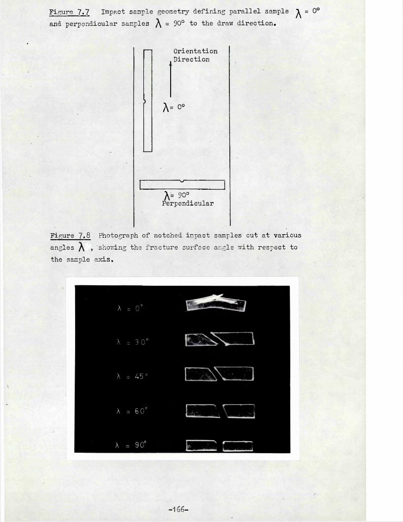
Figure 7.7 Impact sample geometry defining parallel sample ^ = 0° and perpendicular samples ^ = 90° to the draw direction.

Orientation Direction

A = ° °

A= 90°Perpendicular

Figure 7*8 Photograph of notched impact samples cut at various angles , 'showing the fracture surface angle with respect to the sample axis.

Figure 7* 9a. Graph of unnotched impact strengths plotted againstangle \ .

Yielded ©,

0,6J)R-1 ;~X = Bent no fracture

o = Fracture X 6 0'ImpactEnergy

0.3

600 30 50Orientation Angle ^ Degrees

Figure 7.9b. Graph of notched impact strengths plotted againstangle ^ .

ImpactEnergyJ m-3L

o - DR = 2.10.6 -DR = 2.7

600 30

Orientation Angle ^ Degrees

90

CHAPTER EIGHT

SUMMARY AND SUGGESTIONS FOR FURTHER WORK

8.1 Summary

The more important results which have been presented in thisthesis can be summarised as follows:-

1. The magnitude of the compression yield stresses exceeded the magnitude of the tensile yield stresses of the as-received isotropic PVC, over the temperature range -40 -* + 60°C. The ratio of the compressive to tensile yield stresses was 1.2. The non-equality was attributed to the effect of hydrostatic pressure.

2. The effect of increasing orientation on the yield stresses measured in the draw direction was to cause the tensile yield stress to increase rapidly with increasing draw ratio, and since the compressive yield stress was more or less constant, the ratio of the compression to tensile yield stress fell, to

• give values as low as 0,5. The change in yield stress was thought to be due to a *frozen-in* stress in the polymer introduced by hot drawing; the 'frozen-in* stress effect increasing with orientation and exceeding the hydrostatic pressure effect, except at very low Orientations.

3. The variation of the compression yield stress'with ^was■ measured and found to be small with a possible minimum at ^ = 4-5° ; unlike the tensile "yield stress which showed a

-y 7 _ „ minimum at ^ =90° and could show as much as 400% difference between the 0° and 90° yield stresses.

-168-

The Von Mises-Hill yield criterion modified by the ffrozen- in* stress and hydrostatic pressure terms was found to successfully account for the tensile and compression yield

Ud.T'.'J.tion sstress^, both for isotropic and oriented PVC; the angle of formation Of) of the deformation bands could also be predicted. Two strain formulations of the basic Vonrtises criterion with the two correction terms also showed some promise as yield criteria.

The ffrozen-inf stress and its effect on the tensile and compressive yield stresses T/ere esqplained by use of a two phase model of an extended spring held in wax. Release of the ^rozen-in* stress was simulated by the wax softening and melting and allowing the spring to contract.

The elastic constants, compliances and modulus for oriented PVC were measured, using a pulsed ultrasonic transmitting technique. The results showed the same general trends as the results reported in the literature for other materials. A method of comparing degree of orientation of different polymers by plotting

was found useful. The variation of the elastic^ max

constants and the birefringence could be explained by a two- phase aggregate model used previously by Ward for polyethylene.

The influence of orientation on the fracture and impact behaviour, was quite marked, in general weakening along the molecular alignment direction and toughening across the molecules.Fracture surfaces tended to run parallel to the molecules. The oriented PVC had a yield fracture transition at room temper­ature, whereas the isotropic PVC remains ductile to about -50°C. Drawing temperature had some effect on brittleness; it was

observed that drawing at 90°C the PVC was brittle at lower birefringence than PVC drawn at 80°C.

8, The thermal properties were found to be anisotropic in the oriented PVC, and the Tg was reduced by up to 6°C in the highly oriented polymer.

8.2 Future work

The following suggestions are made for possible future linesof investigation:-

1) Determination of the tensile and compression yield stresses on the same oriented material.

2) Determine the effect of hydrostatic pressure on the yield stress, to give further data to check the hydrastatic term in the Kill criterion.

3) Make further measurements of the strain at yield in theoriented PVC so that the modulus and yield stress relation­ship and the strain yield criterion can be probed further.

. k n4) Examine the effect of orientation on the thermal properties,particularly the Tg and the release of *frozen-in* stress with heating. Dielectric or radio frequency heating could be a method of rapidly raising the temperature to above Tg, uniformly through the thickness of a sample, and so minimise the stress decay with slowly increasing temperature that occurs with conductive heating.

5) Further work needs to be done on the relationship betweenfracture properties of oriented PVC and the degree anddirection of orientation. Further use of impact tests would

... ■ , \ • give much useful information.

-170- .

ACKN0Y/L3D&2J5ENTS

I would like to thank -

My supervisor, Dr, J. G. Rider, for suggesting this project, and for his constant guidance and interest throughout the period of this research.

The Ministry of Technology for providing financial support.

The Director of the National Physical Laboratories, and Mr. M. F. Markham for use of their ultrasonic test facilities.

The Director of the Institute of Polymer Technology, Loughborough University, for use.of various research facilities.

Mrs. G. Smith for writing and operating the computer programmes.

Dr. S. Hargreaves and other colleagues at Surrey and Loughborough for many helpful discussions.

Dr. L. E. Miller, Dr. M. Gilbert, and my parents for constant encouragement and for reading the draft of this thesis.

-171-

REFERENCES

1. Musgrave, M.J.P., Crystal Acoustics (San Francisco, etc.:Holden-Day, 1970)

2. Johnson, W. and Mellor, P.B., Plasticity for MechanicalEngineers (D. Van Nostrand Co.Ltd., London, 1962).

3. Vincent, P.I. Polymer, 13, 558-560 (1972).4. Miller, L.3., Puttick, L.C., and Rider, J.G-. J. Poly Sci.C .

33, 13-22 (1971).5. Hill, R., The mathematical theory of plasticity, (Oxford

University Press, London, 1950)6. Brown, N., Duckett, R. A., and Ward, I.M. Phil. Mag. 18,

483 (1968).7. Rider, J.C., and Hargreaves, E., J. Phy. D. Appl. Phy. 3

993-1008 (1970).8. Hargreaves, E., Ph.D. Thesis, University of Surrey, (1970).9. Kuhn, Yf., and Griin, F., Kolloidz.schr., 101, 248, (t$!+2\.10. Rider, J.C., and Hargreaves, E. J. Poly. Sci. A.2, 7,

828 (1969).11. Vincent, P.I., the Encyclopaedia of Polymer Science and

Technology, (John 77iley, New York, 1967, 7, 292).12. Thomas, K., Meyer, D.E., Fleet, E.C., and Abraham, M. ■

J. Phy. D. Appl. Phy. i6, 1336-1361, (1973).13. Hinton, T. Private Communication.14. Evans, J.M. Rapra Bulletin, Nov.1^72 (334-341)15. Curtis, J.W., J. Phy. D., Appl. Phy. 3, 1413-1422, (1970).16. Brundru, J., and Immergat,E.;Polymer Handbook, V/iley Interscience

(19a).

17. Treloar, L.R.G., The Physics of Rubber Elasticity,(Oxford at the Clarendon Press, 1958.)

18. Musgrave, M.J.P., Proc. Phy. Soc., A226, 339 (1954).

-172- .

19* Musgrave, M.J.P., Proc. Phy, Soc., A226, 306 (195 -)20. Markham, M.F., Composites, 1, 145-149, ( i 970)21 . . Wright, H., Faraday, G.S.M., White, E.F.T., and Treloar, L.R.G.

J. Phys. D: Appl. Phys. 4, 2002-2014 (1971j•22. Bridle, C., Buckley, A., and Scanlon, J., J. Mat. Sci., 1_8,

1151 (1967).23. Reynolds, W.N., International Conf. on Carbon Fibres,

London, Paper .No. 52 (1971).24. Reynolds, 7/.N., Plastics and Polymers, 1£, 155-157, (1969).25. Jaeger, J. C., Elasticity, Fracture and Flow, Methuen*s

Monograph, (1954).26. Koshiwagi, M., Folkes, M.J., and Y/ard, I.M., Polymer, 12,

697-710, (1971).27. Horsley, R., Inst. Phy. Conference, Buxton, 1972.28. Robertson, R.E., General Electric Research Laboratories,

Schenectady, New York, 1964, Report No.64-RL-(3580 c).

29. Mills, N., Yield, deformation and fracture conference,Cambridge, 1973*

-30. Duckett, R.A., Yfard, I.M., and Zihlief, A.M., J. Mat. Sci.,7, 480, (1970).

31. Raumann, G., and Saunders, D.W., Proc. Phy. Soc., 77,1028-37, (1961).

32. Kaumann, 0., J. Appl. Phy., 14, 795r798, (1963).33. Vincent, P.I. Impact tests and service performance of

thermoplastics (Plastics Institute, 1971).34. -Allison, S.W., and Ward, I.M., Brit. J. Appl. Phy., 18,

1151, (1967).35. Diniwell, A.E., Project report, Physics Dept., University of

Surrey, (1971).

: -173- ' :

36. Patterson, P.M., Project report, Physics Dept., University ofSurrey, 1972.

37. Andrews, E.H., Fracture in Polymers, Oliver & Boyd, (1968).38. Rawson, F.F., and Rider, J.G., J. Poly. Sci. (c), 33,

87-99, (1971).39* Rawson, F.F., and Rider, J.G., Polymer, 13, (107-110) (1974)40. Rider, J.G., Min. Tec. Report AT/1004/04/NPL, (1972).41. Hawaii, R.N,, Murphy, B.M., and White, E.F.T., J. Poly. .Sci.,

A-2, 9, 801-814, (1971).42. Nadai A., Theory of Flow and Fracture of Solids, Vol. 1,

2nd Ed. McGraw-Hill, New York, 1930.43* Nye, J.F., Physical Properties of Crystals (Oxford:

Claren<3-on Press, 1957).44. Rawson, F.F., and Rider, J.G., J. Phy. D: Appl. Phy., 25,

41-49, (1974).45. Rabinowitz, S., Ward, I.M., and Perry, S.3.C., J. Mat. Sci.

5, 29-39., (1970).46. Gupta,V.3., & Ward, I.M.J., Macromol. Sci. (phy.), B1 (2)

373-400 (1967).47* Ward, I.M., Proc. Phys. Soc. 80, 1176—1188 (1962)• 'V '48. Bauwens, J. C., J. Polymer Sci., A-2, 8, 893 (l970).49. Bauwens - Crowet, J., Bauwens, J.C., Homes, G., J.Mat. Sci.

7, 176-183 (1972).50. Moore, J.C., J. Poly. Sci., A-2, 3, 835-843 (1984).51. Bueche, A.M., J. Poly. Sci., 1_9, 297-306 (1958).52. Haward, R.N., and Thackery, G-., Proc. Roy. Soc., A.302

453 (1988).53* Pinnock, P.R., Ward, I.M., Trans. Faraday Soc., 62, 1308

(1962).54. Ward, I,M., Mechanical properties of solid polymers.

John Wiley, (1971).-174-

55* Penny, M.T., M.Sc. Thesis, Loughborough University, 1971 J56. Stafford., T. G., RAPRA Tec. Review 66, (l972^57. Harrison, M.A., Morgan, P.H., and Park U.S., Br. Poly. J.

8, (1971), p 154. ;58. Walter, A. T. J.. Poly. Soi., 1J5, 954),P 207.59. Gray, A. Private communication.60. Treloar, L.R.G., Introduction to Polymer Science,

Wykeham Science Services, (1970).61. Whitney, W., Andrews, R.D., J. Poly. Sci., 16. 1967^P 2981.

-175-