Degree project in

Solid Mechanics

Second level, 30.0 HEC

Stockholm, Sweden 2011

Thibaud Denoyelle

Mechanical properties of

materials made of

nano-cellulose

2

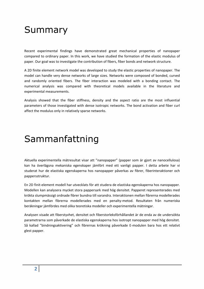
Summary

Recent experimental findings have demonstrated great mechanical properties of nanopaper

compared to ordinary paper. In this work, we have studied the formation of the elastic modulus of

paper. Our goal was to investigate the contribution of fibers, fiber bonds and network structure.

A 2D finite element network model was developed to study the elastic properties of nanopaper. The

model can handle very dense networks of large sizes. Networks were composed of bonded, curved

and randomly oriented fibers. The fiber interaction was modeled with a bonding contact. The

numerical analysis was compared with theoretical models available in the literature and

experimental measurements.

Analysis showed that the fiber stiffness, density and the aspect ratio are the most influential

parameters of those investigated with dense isotropic networks. The bond activation and fiber curl

affect the modulus only in relatively sparse networks.

Sammanfattning

Aktuella experimentella mätresultat visar att ”nanopapper” (papper som är gjort av nanocellulosa)

kan ha överlägsna mekaniska egenskaper jämfört med ett vanligt papper. I detta arbete har vi

studerat hur de elastiska egenskaperna hos nanopapper påverkas av fibrer, fiberinteraktioner och

pappersstruktur.

En 2D finit-element modell har utvecklats för att studera de elastiska egenskaperna hos nanopapper.

Modellen kan analysera mycket stora pappersark med hög densitet. Papperet representerades med

krökta slumpmässigt ordnade fibrer bundna till varandra. Interaktionen mellan fibrerna modellerades

kontakten mellan fibrerna modellerades med en penalty-metod. Resultaten från numeriska

beräkningar jämfördes med olika teoretiska modeller och experimentella mätningar.

Analysen visade att fiberstyvhet, densitet och fiberstorleksförhållandet är de enda av de undersökta

parametrarna som påverkade de elastiska egenskaperna hos isotropt nanopapper med hög densitet.

Så kallad ”bindningsaktivering” och fibrernas krökning påverkade E-modulen bara hos ett relativt

glest papper.

3

Acknowledgement

The work presented in this master thesis has been carried out at the Department of Solid Mechanics

and the Wallenberg Wood Science Center (WWSC), Royal Institute of Technology (KTH), Stockholm

between August 2010 and January 2011. They are gratefully acknowledged for their support.

First of all, I would like to express my sincere gratitude to my supervisor Professor Artem Kulachenko

for giving me the opportunity to take part of his project. I am deeply thankful for your precious

advises and excellent guidance through this project but also for your kindness and good relationships

further the work time.

Further thanks to Prof. Lars Berglund for his interesting comments and discussions all the way along

the project.

Mr. Sylvain Galland, Mrs. Elina Mabasa Bergström and Mrs. Michaela Salajkova are gratefully

acknowledged for their help in the laboratory. I really appreciate your help and the time you spent

during the experimental part of my project.

I am also thankful to all the people and friends who took part to this “Swedish adventure”. First of all,

many thank to people who help me to finalize this project. I also would like to thank you all my

friends for making this experience enjoyable and their contribution to a stimulating environment.

4

Table of Contents

1. General introduction ........................................................................................................................... 6

2. Paper: from the cellulose fiber to a simple sheet ............................................................................... 8

2.1 The cellulose: the main component of paper ............................................................................... 8

2.1.1 Structure of cellulose ............................................................................................................. 8

2.1.2 Mechanical properties of the cellulose .................................................................................. 9

2.2 The paper making process ........................................................................................................... 10

2.2.1 The pulping process .............................................................................................................. 10

2.2.2 How to make a sheet of paper? ........................................................................................... 11

2.3 Mechanical properties of paper .................................................................................................. 12

2.3.1 Different ways to obtain cellulose fiber ............................................................................... 13

2.3.2 Structural imperfections ....................................................................................................... 14

3. Theoretical network models ............................................................................................................. 17

3.1 The Cox model ............................................................................................................................. 17

3.2 The Shear-lag model .................................................................................................................... 18

3.3 The effective medium model ...................................................................................................... 19

3.4 A comparison with experimental results .................................................................................... 20

3.4.1 The experimental results ...................................................................................................... 20

3.4.2 Comparing the results .......................................................................................................... 21

4. The finite element model .................................................................................................................. 24

4.1 The network ................................................................................................................................ 24

4.1.1 The fibers .............................................................................................................................. 24

4.1.2 Geometry of the network ..................................................................................................... 27

4.2 The boundary conditions ............................................................................................................. 29

4.3 Convergence ................................................................................................................................ 30

4.3.1 The meshing convergence .................................................................................................... 30

4.3.2 The size convergence ........................................................................................................... 31

5. The Results ........................................................................................................................................ 33

5.1 An homogeneous network .......................................................................................................... 33

5.2 Effect of the density .................................................................................................................... 34

5.3 Dimensions of the fibers ............................................................................................................. 35

5

5.4 Influence of curled fibers and bonds ........................................................................................... 37

5.4.1 The influence of the bonds ................................................................................................... 37

5.4.2 Influence of curled fibers ..................................................................................................... 42

6. Experimental section ......................................................................................................................... 47

6.1 How to obtain NFC films? ............................................................................................................ 47

6.2 The experiments .......................................................................................................................... 49

6.2.1 The density and dimensions of the sample. ......................................................................... 49

6.2.2 The elastic modulus .............................................................................................................. 50

6.2.3 Fibers’ aspect ratio ............................................................................................................... 51

6.3 Experimental results .................................................................................................................... 52

6.3.1 The density ........................................................................................................................... 53

6.3.2 The dimensions of the fibers ................................................................................................ 54

6.3.3 The elastic modulus .............................................................................................................. 55

7. Concluding remarks ........................................................................................................................... 58

7.1 Summary and conclusion ............................................................................................................ 58

7.2 Future work ................................................................................................................................. 59

Bibliography ........................................................................................................................................... 60

Table of panels ...................................................................................................................................... 62

Table of figures ...................................................................................................................................... 63

A: Derivation of the Cox relation ........................................................................................................... 66

B: Derivation of the Shear-lag relation .................................................................................................. 68

C: Derivation of the Poissonian model formula .................................................................................... 70

D: Preparing a sample ........................................................................................................................... 72

6

1. General introduction

Nowadays, the world population is reaching seven billions of humans and, according to the current

projections, the population is expected to reach 10.5 billion in 2050. The rapid increase of the human

population during the 20th century accompanying with a rise in usage of fossil fuels are both

responsible for the increasing cost of crude oil and ecological threats such as global warning and

pollution.

In this economical and ecological context, renewable and biodegradable materials have been

receiving, for several years, more and more attention from the scientific community. Indeed, many

material systems found in nature exhibit combinations of properties not currently found in synthetic

systems.

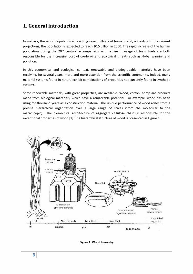
Some renewable materials, with great properties, are available. Wood, cotton, hemp are products

made from biological materials, which have a remarkable potential. For example, wood has been

using for thousand years as a construction material. The unique performance of wood arises from a

precise hierarchical organization over a large range of scales (from the molecular to the

macroscopic). The hierarchical architecture of aggregate cellulose chains is responsible for the

exceptional properties of wood [1]. The hierarchical structure of wood is presented in Figure 1.

Figure 1: Wood hierarchy

7

Wood exhibits great mechanical properties, mainly due to cellulose polymer chains. Crystalline

cellulose is the reinforcing constituent component of wood cells. It is also one of the most abundant

biopolymers on earth with a total quantity of approximately 1011 tons [2]. Due to its abundance, high

strength and stiffness, low weight and biodegradability, the industrial use of cellulose is widespread

in the present age, mainly for making paper and board. All the different steps to produce ordinary

paper from wood are presented in Figure 2. The type of fibers used for these applications are

microfibril cellulose fibers. Due to the presence of hemicellulose, amorphous cellulose and defects

induce by the extraction process, the mechanical properties of the microfibrils are very low

compared to pure crystalline cellulose.

Using the same hierarchical structures existing in wood is a way to have products with higher

biomechanical features. Since recently, it has become quite easy to produce nanofibrilated cellulose

(NFC) in laboratory scale. The smaller dimensions, a higher crystallinity and a large surface area of

NFC compare to microfibril open new ways to use cellulose-based materials.

Despite major advantages of nano-cellulose such as its nontoxicity [3], broad availability and great

mechanical properties, its use is r to niche applications. Its moisture sensitivity, its incompatibility

with oleophilic polymers and the high energy consumption needed to produce NFC prevent them to

compete with other mass products such as ordinary paper or plastic. However, NFC has been already

used for several purposes such as polymer reinforcement [4] or antimicrobial films [5].

Little has been reported about the use of NFC in paper applications but recent experiments have

shown the great mechanical properties of nanopaper compared to ordinary paper [6,7], the

motivation of this thesis is to estimate the potential of pure NFC films. Our goal was to investigate

the contribution of fibers and network structure and how it changes as the scale of raw material

shifts from mm-micro level (fibers in conventional paper) to micro-nano level (cellulose nanofibrils in

nanopaper).

Figure 2: The paper making process

8

2. Paper: from the cellulose fiber to a simple sheet

Paper is a thin material mainly used for printing and packaging. It is obtained by pressing together

moist cellulose fiber and then drying them into flexible sheets. Even if some components are added,

cellulose fibers can be considered as the only constitutive element of paper.

2.1 The cellulose: the main component of paper

As mentioned before, cellulose is probably one of the most ubiquitous and abundant polymers on

the earth. It is a dominant reinforcing phase in plant structures (See Table 1).

Table 1: Amount of cellulose in some common plants

Plant % of cellulose fibers (volume)

Cotton 82.7 Jute 64.4

Lin 64.1

Ramie 68.6

Sisal

65.8

Wood 40-45

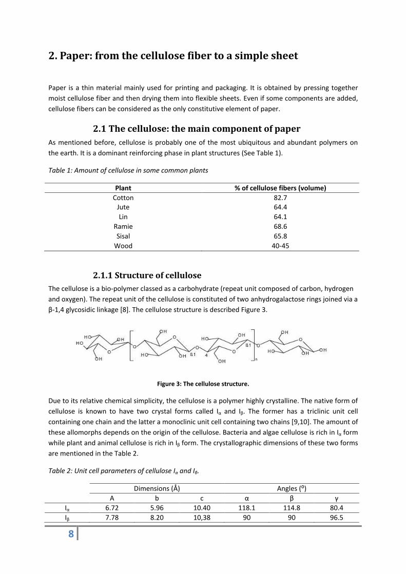
2.1.1 Structure of cellulose

The cellulose is a bio-polymer classed as a carbohydrate (repeat unit composed of carbon, hydrogen

and oxygen). The repeat unit of the cellulose is constituted of two anhydrogalactose rings joined via a

β-1,4 glycosidic linkage [8]. The cellulose structure is described Figure 3.

Figure 3: The cellulose structure.

Due to its relative chemical simplicity, the cellulose is a polymer highly crystalline. The native form of

cellulose is known to have two crystal forms called Iα and Iβ. The former has a triclinic unit cell

containing one chain and the latter a monoclinic unit cell containing two chains [9,10]. The amount of

these allomorphs depends on the origin of the cellulose. Bacteria and algae cellulose is rich in Iα form

while plant and animal cellulose is rich in Iβ form. The crystallographic dimensions of these two forms

are mentioned in the Table 2.

Table 2: Unit cell parameters of cellulose Iα and Iβ.

Dimensions (Å) Angles (:)

A b c α β γ

Iα 6.72 5.96 10.40 118.1 114.8 80.4

Iβ 7.78 8.20 10,38 90 90 96.5

9

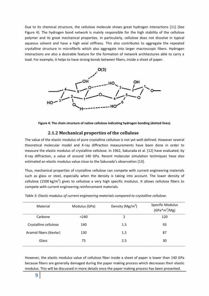
Due to its chemical structure, the cellulose molecule shows great hydrogen interactions [11] (See

Figure 4). The hydrogen bond network is mainly responsible for the high stability of the cellulose

polymer and its great mechanical properties. In particularly, cellulose does not dissolve in typical

aqueous solvent and have a high axial stiffness. This also contributes to aggregate the repeated

crystalline structure in microfibrils which also aggregate into larger macroscopic fibers. Hydrogen

interactions are also a desirable feature for the formation of network architectures able to carry a

load. For example, it helps to have strong bonds between fibers, inside a sheet of paper.

Figure 4: The chain structure of native cellulose indicating hydrogen bonding (dotted lines).

2.1.2 Mechanical properties of the cellulose

The value of the elastic modulus of pure crystalline cellulose is not yet well-defined. However several

theoretical molecular model and X-ray diffraction measurements have been done in order to

measure the elastic modulus of crystalline cellulose. In 1962, Sakurada et al. [12] have evaluated, by

X-ray diffraction, a value of around 140 GPa. Recent molecular simulation techniques have also

estimated an elastic modulus value close to the Sakurada’s observation [13].

Thus, mechanical properties of crystalline cellulose can compete with current engineering materials

such as glass or steel, especially when the density is taking into account. The lower density of

cellulose (1500 kg/m3) gives to cellulose a very high specific modulus. It allows cellulose fibers to

compete with current engineering reinforcement materials.

Table 3: Elastic modulus of current engineering materials compared to crystalline cellulose.

Material Modulus (GPa) Density (Mg/m3) Specific Modulus

(GPa*m3/Mg)

Carbone >240 2 120

Crystalline cellulose 140 1.5 93

Aramid fibers (Kevlar) 130 1.5 87

Glass 75 2.5 30

However, the elastic modulus value of cellulose fiber inside a sheet of paper is lower than 140 GPa

because fibers are generally damaged during the paper making process which decreases their elastic

modulus. This will be discussed in more details once the paper making process has been presented.

10

2.2 The paper making process

The paper making process is very old (according to historians, Chinese people already use it in AD

105) but the manufacture of paper became an industrial reality at the beginning of the 19th. Since

only the cellulose is needed to obtain a paper, the first step (in most cases), is to extract cellulose

from the wood.

The structure of wood consists on a thin primary wall and three secondary layers (S1, S2, and S3)

[14]. Each layer is composed of cellulose fibers, a bio polymer, mainly crystalline, surrounded by an

amorphous matrix of hemicellulose and lignin [15]. The cellulose is the major component in wood

with a volumetric content ranging from 40% to 45%. As for the hemicellulose and the lignin, each of

them represents, approximately, 30% of the total volume. Due to the low mechanical properties of

the lignin and the hemicellulose, these are the cellulose fibers which give wood its great mechanical

behavior. Figure 5 and 6 present the arrangement of cellulose fibers.

Figure 5: A single wood fiber with the arrangement

of the cellulose in the different layers.

Figure 6: Schematic arrangement of the cellulose

fiber inside a layer.

2.2.1 The pulping process

The first step is to separate the other materials from the cellulose to obtain a substance called wood

pulp. This process is called “pulping”. There are several pulping processes but only two are widely

used. There are:

the mechanical process;

the chemical process.

In the mechanical process, the logs are grinding with a moisture content of 45-50% to separate the

cellulose fibers from the rest. Mechanical pulping is very efficient and can convert 90% of the wood

into pulp but this pulp contains most of the constituents of the wood. Generally, chemicals aid the

mechanical grinding.

11

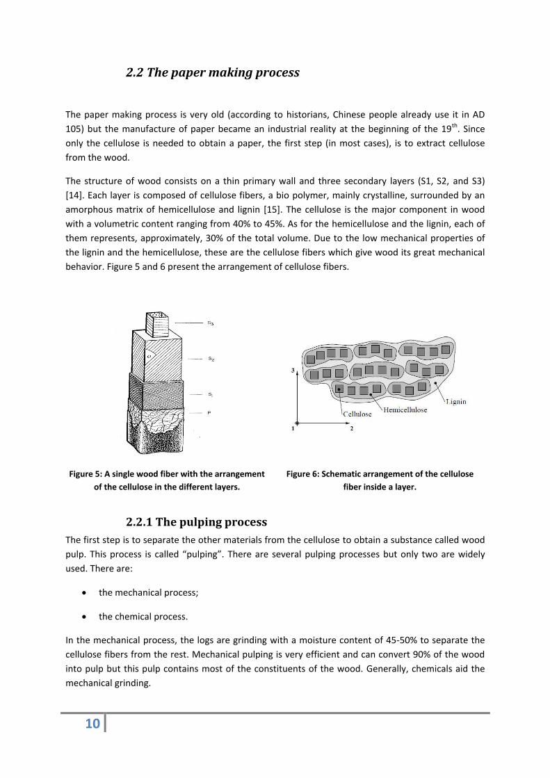
In the chemical process, chemicals, heat and pressure are used to dissolve the lignin and to free the

cellulose fibers from the matrix. The process, also called the “Kraft process”, removes sugars and

approximately 95% of the lignin in the final product. The “Kraft" process is presented Figure 7.

Figure 7: Action of sodium hydroxide and sodium sulfite to break down the lignin (”Kraft" process).

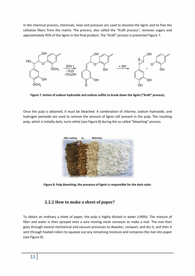
Once the pulp is obtained, it must be bleached. A combination of chlorine, sodium hydroxide, and

hydrogen peroxide are used to remove the amount of lignin still present in the pulp. The resulting

pulp, which is initially dark, turns white (see Figure 8) during the so called “bleaching” process.

Figure 8: Pulp bleaching; the presence of lignin is responsible for the dark color.

2.2.2 How to make a sheet of paper?

To obtain an ordinary a sheet of paper, the pulp is highly diluted in water (≈99%). The mixture of

fiber and water is then sprayed onto a wire moving mesh conveyor to make a mat. The mat then

goes through several mechanical and vacuum processes to dewater, compact, and dry it, and then it

sent through heated rollers to squeeze out any remaining moisture and compress the mat into paper

(see Figure 9).

12

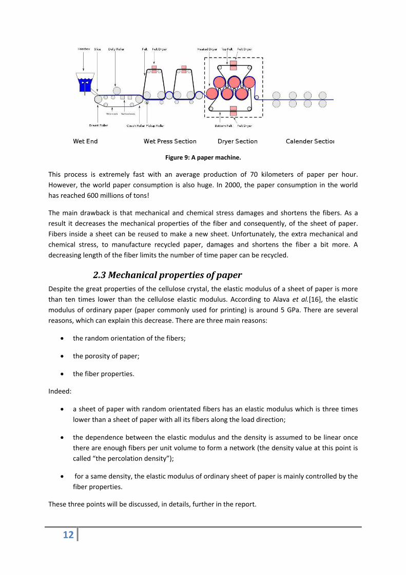
Figure 9: A paper machine.

This process is extremely fast with an average production of 70 kilometers of paper per hour.

However, the world paper consumption is also huge. In 2000, the paper consumption in the world

has reached 600 millions of tons!

The main drawback is that mechanical and chemical stress damages and shortens the fibers. As a

result it decreases the mechanical properties of the fiber and consequently, of the sheet of paper.

Fibers inside a sheet can be reused to make a new sheet. Unfortunately, the extra mechanical and

chemical stress, to manufacture recycled paper, damages and shortens the fiber a bit more. A

decreasing length of the fiber limits the number of time paper can be recycled.

2.3 Mechanical properties of paper

Despite the great properties of the cellulose crystal, the elastic modulus of a sheet of paper is more

than ten times lower than the cellulose elastic modulus. According to Alava et al.[16], the elastic

modulus of ordinary paper (paper commonly used for printing) is around 5 GPa. There are several

reasons, which can explain this decrease. There are three main reasons:

the random orientation of the fibers;

the porosity of paper;

the fiber properties.

Indeed:

a sheet of paper with random orientated fibers has an elastic modulus which is three times

lower than a sheet of paper with all its fibers along the load direction;

the dependence between the elastic modulus and the density is assumed to be linear once

there are enough fibers per unit volume to form a network (the density value at this point is

called “the percolation density”);

for a same density, the elastic modulus of ordinary sheet of paper is mainly controlled by the

fiber properties.

These three points will be discussed, in details, further in the report.

13

2.3.1 Different ways to obtain cellulose fiber

With the cellulose fibers extracting from wood, depending on the pulping process, various

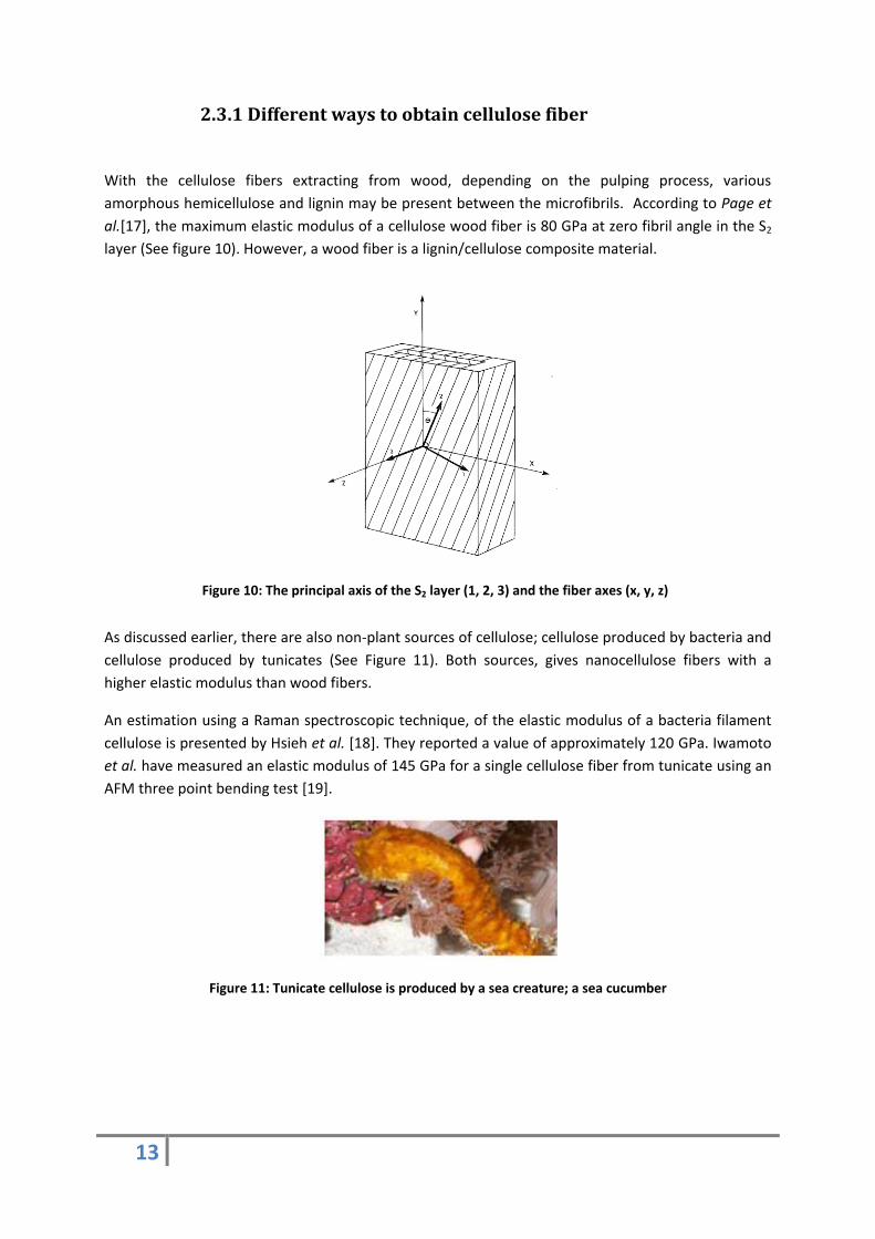
amorphous hemicellulose and lignin may be present between the microfibrils. According to Page et

al.[17], the maximum elastic modulus of a cellulose wood fiber is 80 GPa at zero fibril angle in the S2

layer (See figure 10). However, a wood fiber is a lignin/cellulose composite material.

Figure 10: The principal axis of the S2 layer (1, 2, 3) and the fiber axes (x, y, z)

As discussed earlier, there are also non-plant sources of cellulose; cellulose produced by bacteria and

cellulose produced by tunicates (See Figure 11). Both sources, gives nanocellulose fibers with a

higher elastic modulus than wood fibers.

An estimation using a Raman spectroscopic technique, of the elastic modulus of a bacteria filament

cellulose is presented by Hsieh et al. [18]. They reported a value of approximately 120 GPa. Iwamoto

et al. have measured an elastic modulus of 145 GPa for a single cellulose fiber from tunicate using an

AFM three point bending test [19].

Figure 11: Tunicate cellulose is produced by a sea creature; a sea cucumber

14

Thus, different sources of cellulose fibers provide different elastic modulus values. Regarding the

mechanical properties of the sheet of paper, non-plant cellulose fibers have also the advantages to

be “ready to use”. That means that fibers are obtained directly and can be used directly to

manufacture a sheet of paper. Consequently, such fibers are, more or less, free of damages contrary

to cellulose fibers extract from wood. Structural imperfections and damages are induced into the

cellulose wood fibers during the papermaking process.

2.3.2 Structural imperfections

The S2-layer holds the fibers together in the wood material. This layer is removed, partly or completely, during the papermaking process. Unfortunately, the fiber structure may also suffer several mechanical damages. Several imperfections are induced in the fibers during the papermaking process. Suspension flow and drainage on the wire create curl, twist, dislocations and pressing undulations in the sheet [16]. The impact of these various states on the fiber elastic modulus has been well described by Page and Seth [20-21].

2.3.2.1 The fiber length

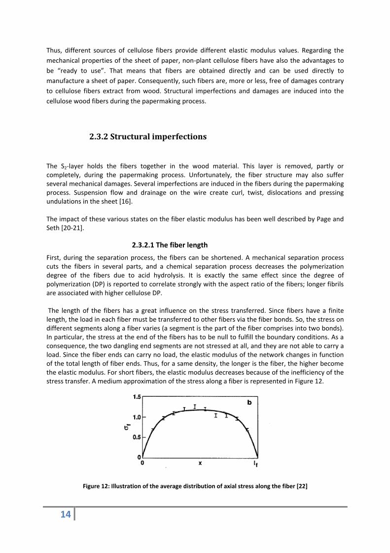
First, during the separation process, the fibers can be shortened. A mechanical separation process cuts the fibers in several parts, and a chemical separation process decreases the polymerization degree of the fibers due to acid hydrolysis. It is exactly the same effect since the degree of polymerization (DP) is reported to correlate strongly with the aspect ratio of the fibers; longer fibrils are associated with higher cellulose DP. The length of the fibers has a great influence on the stress transferred. Since fibers have a finite length, the load in each fiber must be transferred to other fibers via the fiber bonds. So, the stress on different segments along a fiber varies (a segment is the part of the fiber comprises into two bonds). In particular, the stress at the end of the fibers has to be null to fulfill the boundary conditions. As a consequence, the two dangling end segments are not stressed at all, and they are not able to carry a load. Since the fiber ends can carry no load, the elastic modulus of the network changes in function of the total length of fiber ends. Thus, for a same density, the longer is the fiber, the higher become the elastic modulus. For short fibers, the elastic modulus decreases because of the inefficiency of the stress transfer. A medium approximation of the stress along a fiber is represented in Figure 12.

Figure 12: Illustration of the average distribution of axial stress along the fiber [22]

15

2.3.2.2 Effects of dislocations, curls, crimps, kinks…

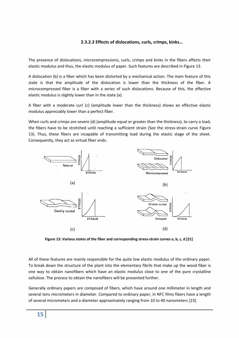
The presence of dislocations, microcompressions, curls, crimps and kinks in the fibers affects their

elastic modulus and thus, the elastic modulus of paper. Such features are described in Figure 13.

A dislocation (b) is a fiber which has been distorted by a mechanical action. The main feature of this

state is that the amplitude of the dislocation is lower than the thickness of the fiber. A

microcompressed fiber is a fiber with a series of such dislocations. Because of this, the effective

elastic modulus is slightly lower than in the state (a).

A fiber with a moderate curl (c) (amplitude lower than the thickness) shows an effective elastic

modulus appreciably lower than a perfect fiber.

When curls and crimps are severe (d) (amplitude equal or greater than the thickness), to carry a load,

the fibers have to be stretched until reaching a sufficient strain (See the stress-strain curve Figure

13). Thus, these fibers are incapable of transmitting load during the elastic stage of the sheet.

Consequently, they act as virtual fiber ends.

(a)

(b)

(c)

(d)

Figure 13: Various states of the fiber and corresponding stress-strain curves a, b, c, d [21]

All of these features are mainly responsible for the quite low elastic modulus of the ordinary paper.

To break down the structure of the plant into the elementary fibrils that make up the wood fiber is

one way to obtain nanofibers which have an elastic modulus close to one of the pure crystalline

cellulose. The process to obtain the nanofibers will be presented further.

Generally ordinary papers are composed of fibers, which have around one millimeter in length and

several tens micrometers in diameter. Compared to ordinary paper, in NFC films fibers have a length

of several micrometers and a diameter approximately ranging from 10 to 40 nanometers [23].

16

In addition to a higher aspect ratio, NFC fibers are also less damaged than ordinary fibers. Indeed, a

smaller size induces smaller defects. Thus, recent measurement [6,7] have shown a remarkably high

elastic modulus of NFC films. They reported values ranging from 10 to 17 GPa. This is several times

higher than the elastic modulus of printing paper. They also reported a tensile strength of nanopaper

2.5 times higher than ordinary paper.

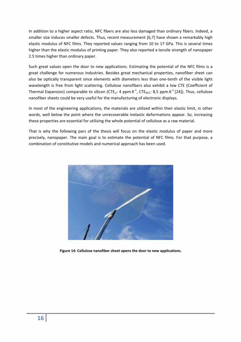
Such great values open the door to new applications. Estimating the potential of the NFC films is a

great challenge for numerous industries. Besides great mechanical properties, nanofiber sheet can

also be optically transparent since elements with diameters less than one-tenth of the visible light

wavelength is free from light scattering. Cellulose nanofibers also exhibit a low CTE (Coefficient of

Thermal Expansion) comparable to silicon (CTEsi: 4 ppm.K-1, CTENFC: 8,5 ppm.K-1 [24]). Thus, cellulose

nanofiber sheets could be very useful for the manufacturing of electronic displays.

In most of the engineering applications, the materials are utilized within their elastic limit, in other

words, well below the point where the unrecoverable inelastic deformations appear. So, increasing

these properties are essential for utilizing the whole potential of cellulose as a raw material.

That is why the following pars of the thesis will focus on the elastic modulus of paper and more

precisely, nanopaper. The main goal is to estimate the potential of NFC films. For that purpose, a

combination of constitutive models and numerical approach has been used.

Figure 14: Cellulose nanofiber sheet opens the door to new applications.

17

3. Theoretical network models

The elastic properties of paper originate primarily from a network of fibers. The stiffness of paper

depends on a number of factors, such as fiber orientation, fiber stiffness and network

interconnectivity (also expressed through density).

Numerous authors have dealt with the problem of elastic modulus of paper. Mathematical equations

have been derived from theoretical consideration of the deformation of a bonded random fibrous

network. Generally, these equations have not been tested adequately by experimental work and the

assumptions, on which the theories are based, are quite simple.

Moreover, predictions of theoretical models are always higher for ordinary paper, since it is

impossible to quantify how damage the fibers are and the proportion of each type of defects (curling,

crimping, etc.). As mentioned previously, such defects are mainly responsible for the low elastic

modulus of printing paper. Now, by decreasing the size of the fibers, we also decrease the size of the

defects which can occur on the fibers (the so-called “scale effect”). This effect is responsible for the

higher mechanical properties of glass fibers compare to bulk glass. So, if we assume that the

nanofibers are free of damages due to a smaller size, the predictions of some theoretical models

should fit better the experimental results.

To compare experimental results and theoretical models, the experimental results of Henriksson et

al. and Syverud et al. [6,7] have been used. Concerning the theoretical models, three network

models based on physical reasoning have been used:

the Cox model;

the Shear-lag model;

the Poissonian model.

Since a sheet of paper, because of a very small thickness (below 100 μm), is closed to a planar mat of

fibers, all of these models are two dimensional.

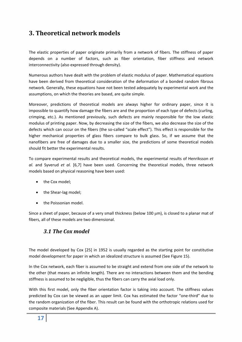
3.1 The Cox model

The model developed by Cox [25] in 1952 is usually regarded as the starting point for constitutive

model development for paper in which an idealized structure is assumed (See Figure 15).

In the Cox network, each fiber is assumed to be straight and extend from one side of the network to

the other (that means an infinite length). There are no interactions between them and the bending

stiffness is assumed to be negligible, thus the fibers can carry the axial load only.

With this first model, only the fiber orientation factor is taking into account. The stiffness values

predicted by Cox can be viewed as an upper limit. Cox has estimated the factor “one-third” due to

the random organization of the fiber. This result can be found with the orthotropic relations used for

composite materials (See Appendix A).

18

Figure 15: A Cox network

For a sheet of paper with a random organization, the upper limit is:

fs EE 3

1 (1)

Where Es and Ef are respectively the elastic modulus of the sheet of paper and the fibers.

Then, a factor has been introduced, by Cox, to take account of the network coverage (the equivalent

of the density in 2D). This factor is the cross section of the fiber (Af) multiply by the length of fiber (q)

per unit area (fiber length is unity) in 2D.

When it comes to three dimensional networks, the factor to take account of the density is the ratio

between the density of the sheet and the density of the fiber in 3D. Thus, the formula becomes [26]:

f

s

fffs EGPaEqAEmNE

3

1)(

3

1)/( (2)

Cox also recognized that in practice, fibers have a finite length, and load is transferred from fiber to

fiber. Thus, Cox introduced the effect of short fibers comparing to infinite fibers in a model called the

Shear-lag theory.

3.2 The Shear-lag model

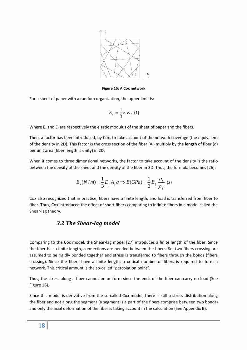
Comparing to the Cox model, the Shear-lag model [27] introduces a finite length of the fiber. Since

the fiber has a finite length, connections are needed between the fibers. So, two fibers crossing are

assumed to be rigidly bonded together and stress is transferred to fibers through the bonds (fibers

crossing). Since the fibers have a finite length, a critical number of fibers is required to form a

network. This critical amount is the so-called “percolation point”.

Thus, the stress along a fiber cannot be uniform since the ends of the fiber can carry no load (See

Figure 16).

Since this model is derivative from the so-called Cox model, there is still a stress distribution along

the fiber and not along the segment (a segment is a part of the fibers comprise between two bonds)

and only the axial deformation of the fiber is taking account in the calculation (See Appendix B).

19

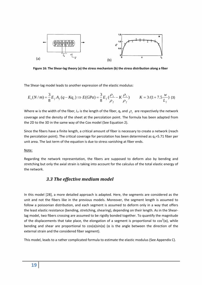
(a) (b)

Figure 16: The Shear-lag theory (a) the stress mechanism (b) the stress distribution along a fiber

The Shear-lag model leads to another expression of the elastic modulus:

)(8

3)()(

8

3)/(

f

c

f

s

fcffs KEGPaEKqqAEmNE

)5.71/(3

fL

wK (3)

Where w is the width of the fiber, LF is the length of the fiber, qc and c are respectively the network

coverage and the density of the sheet at the percolation point. The formula has been adapted from

the 2D to the 3D in the same way of the Cox model (See Equation 2).

Since the fibers have a finite length, a critical amount of fiber is necessary to create a network (reach

the percolation point). The critical coverage for percolation has been determined as qc=5.71 fiber per

unit area. The last term of the equation is due to stress vanishing at fiber ends.

Note:

Regarding the network representation, the fibers are supposed to deform also by bending and

stretching but only the axial strain is taking into account for the calculus of the total elastic energy of

the network.

3.3 The effective medium model

In this model [28], a more detailed approach is adapted. Here, the segments are considered as the

unit and not the fibers like in the previous models. Moreover, the segment length is assumed to

follow a poissonian distribution, and each segment is assumed to deform only in a way that offers

the least elastic resistance (bending, stretching, shearing), depending on their length. As in the Shear-

lag model, two fibers crossing are assumed to be rigidly bonded together. To quantify the magnitude

of the displacements that take place, the elongation of a segment is proportional to cos2(α), while

bending and shear are proportional to cos(α)sin(α) (α is the angle between the direction of the

external strain and the considered fiber segment).

This model, leads to a rather complicated formula to estimate the elastic modulus (See Appendix C).

20

)1)()1(2

13())((

2

8)/( 1

22

zz

ff

f

s ezEz

e

L

qw

L

qwEmNE

(4)

Where

1

1 )( dxxezE zx and fc Lqlz 2 and q represent the number of fiber per unit area

(fiber length is still the unit).

In the model, the bending stiffness modulus is assumed to be 34 lEw , the shear modulus stiffness

lEw 122 and the elongation stiffness modulus lEw2 .

It is also assumed that a segment deforms only by bending if the bending modulus is smaller than

both the shear and the elongation modulus. That mean to have a segment length greater than

)1(2 wlc .

Note:

The average segment length is qLL fmean 2 .

3.4 A comparison with experimental results

In order to investigate the validity of each model, a comparison was made between the theoretical

predictions from the different models stated above and the experimental results obtained by

Henriksson et al. [6] and Syverud et al. [7].

3.4.1 The experimental results

The different samples used by Henriksson and Syverud were made according to the same

preparation process, except for the drying step. The wood-cellulose nanopaper films were prepared

by vacuum filtration of nanoFibrillar Cellulose (NFC) suspension and then dried. If Syverud et al. have

prepared their films by free drying at room temperature, Henriksson et al. dried their films at 55:C at

about 10 kPa applied pressure.

During the drying process, the fibers shrink. According to Salminen et al. [29], the longitudinal and

transversal drying shrinkage potential ( // and ) of the fiber are, respectively, 2% and 20%.

According to a majority of scientists, the drying stress increases the elastic modulus of single fibers

and thus the elastic modulus of the sheet. The drying stress prevents the fiber from buckling and

numerous segments become activated. That means, segments are straightened and ready to carry a

load.

21

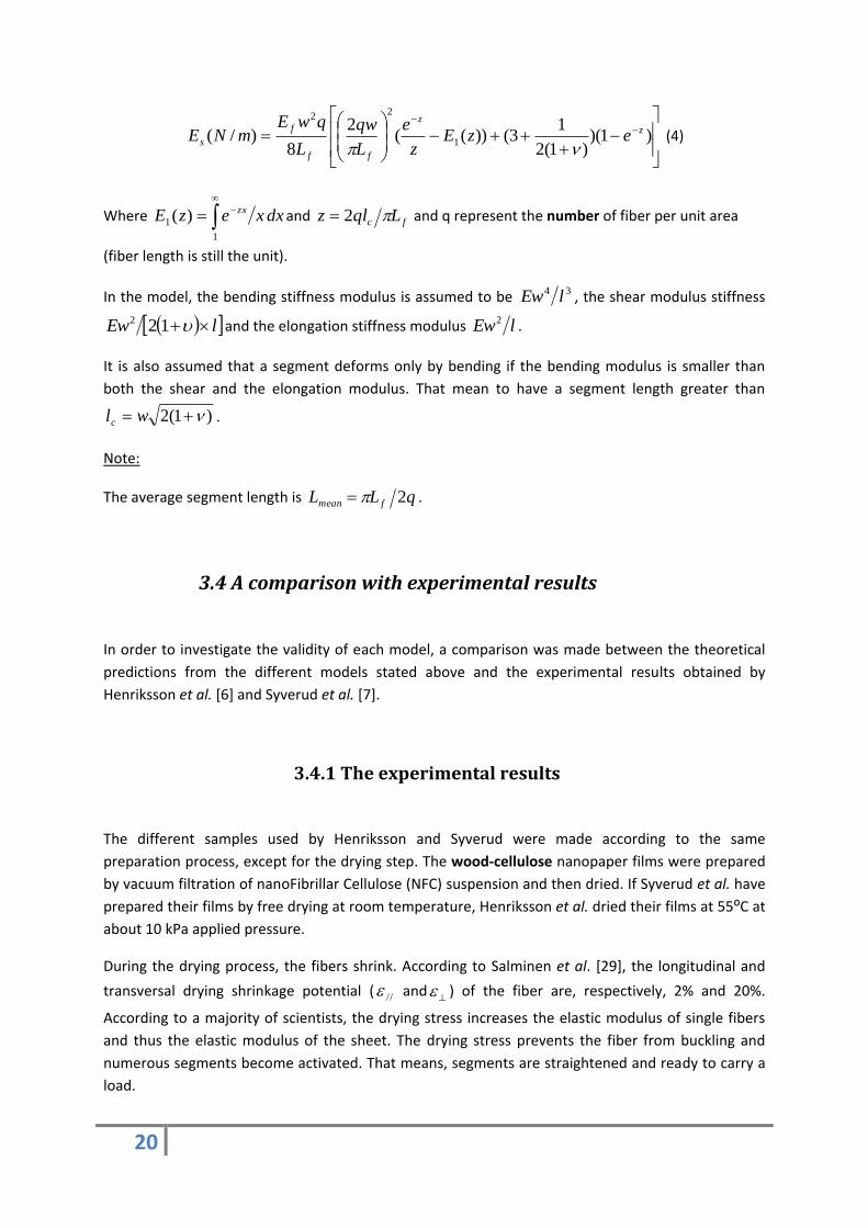
So, normally, the results from Henriksson et al. should be higher than the ones obtained by Severud

et al. Surprisingly, this is not the case. The experimental results are presented in Figure 17.

Figure 17: Comparison of the experimental results.

For the same porosity, the elastic modulus value of Severud et al. can be three times higher than

those obtained by Berglung et al. Thus, it clearly appears that we will be not able to find a theoretical

model which can describe these experimental results. Indeed, none of the theoretical models

predict the influence of drying and the dimensions of the fibers are missing in the article from

Severud et al..

Note:

With the results obtained by Henriksson, we can notice interesting result points (Indicate by 1, 2,

and 3). One can see that two sheets of paper have the same porosity but a different elastic modulus.

There are also two films with the same elastic modulus but having a different density.

In the two cases, the average polymerization degree (DP) of the fiber is different. The higher is the

DP, the longer is the fiber. The points 1, 2 and 3 correspond respectively to a DP of 800, 580 and

1100. Thus, the dimensions of the fibers have an influence of the elastic properties of our network.

3.4.2 Comparing the results

Although, there is a large difference between the results, we can still try to see which models fit the

results best.

For that purpose, we made some assumptions for the calculations. We assumed that the elastic

modulus of all the fiber inside the sheet has an elastic modulus equal to 80 GPa, a length equal to 5

μm and a width and thickness both equal to 50 nm. These are quite common values in the literature.

The elastic modulus of 80 GPa is in the lower part of values available for cellulose nanofibers while

the length of the fibers can be considered as a high assumption.

1 2

3

22

We also assumed to have a square cross section. Thus, it is possible to have a relationship between q

and in the Poissonian model. For a square beam, we have:

f

f

f

s

ffff

ffs

w

L

tLw

tLq

2

(5)

Where q is the number of fiber per unit area, s the density of the sheet and f the density of the

fiber. Lf, wf and tf are respectively the length, width and thickness of the fiber.

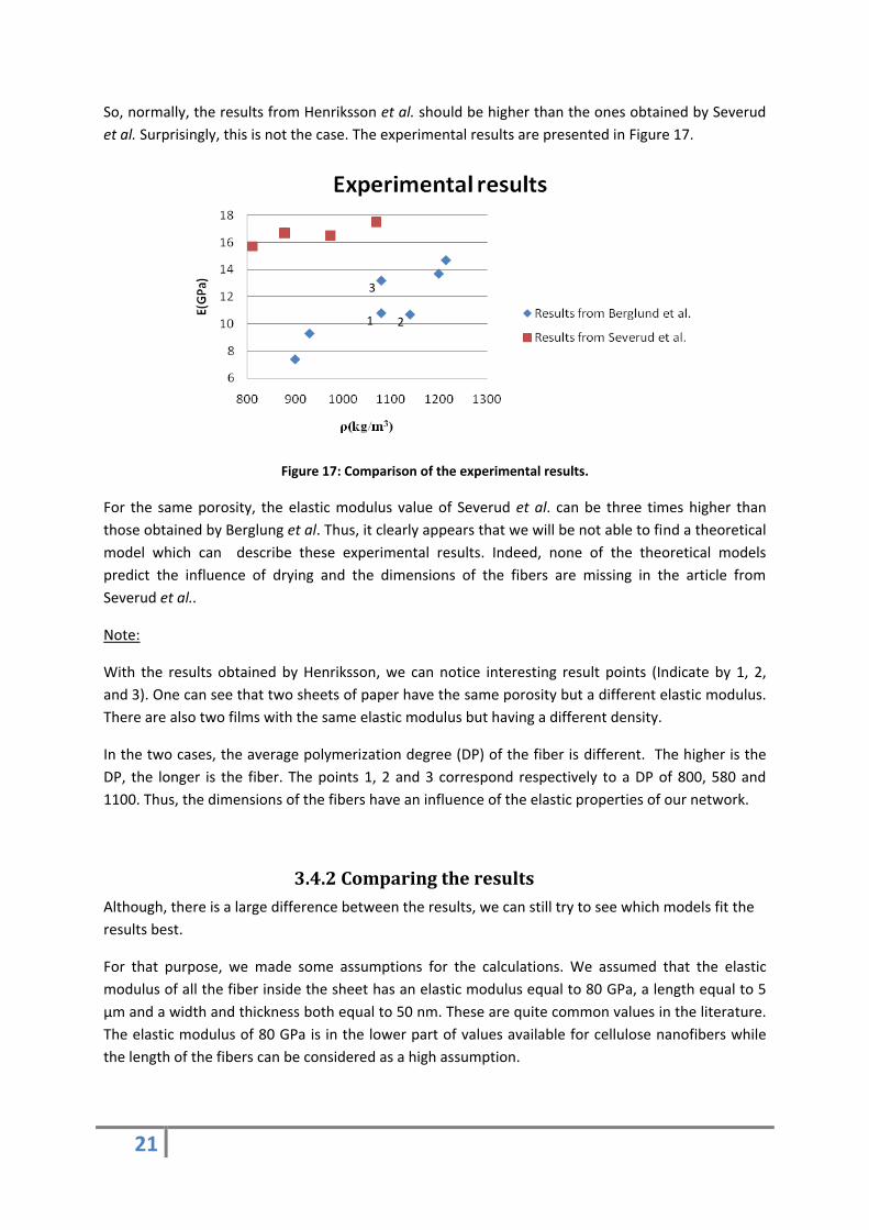
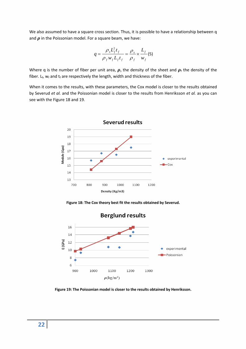
When it comes to the results, with these parameters, the Cox model is closer to the results obtained

by Severud et al. and the Poissonian model is closer to the results from Henriksson et al. as you can

see with the Figure 18 and 19.

Figure 18: The Cox theory best fit the results obtained by Severud.

Figure 19: The Poissonian model is closer to the results obtained by Henriksson.

23

With the results, it clearly appears that a model assessment is impossible. It is impossible to know,

with a great accuracy, the fibers’ elastic modulus, length and width inside the sheet of paper.

Moreover, these theories are unable to describe the eventual presence of fiber defects.

Furthermore, the deviation of the different experimental results can be explained by the difficulty of

these measurements. Since a sheet of paper has a very small thickness, it is impossible to know with

a great accuracy the cross section of the sheet. As a consequence, it is quite complicated to obtain a

precise elastic modulus value. Measuring the density of paper is also a formidable task and thus

experimental verification of any model based on density is difficult. However, in modeling the density

of a sheet of paper is known with a great accuracy.

The experimental results from Henriksson predict also a dependence between the elastic modulus

value of the network and the ratio between the length and the width of the fibers. Only the Shear-lag

model captures such a behavior. Our calculations with the Poissonian model are insensitive to the

ratio. That is why this model will be no longer mentioned in the thesis.

However, having a great accurate estimation of fiber elastic modulus, length and width can be done

with modeling.

With modeling, we will still not be able to predict experimental results since it is impossible know the

properties of the fibers inside a sheet. However, a model is the only way to see how a single

parameter can affect the elastic properties of a fiber network. It shows how the network behaves in

function of the different parameters. It is very useful to find which parameters are really important

to obtain a nanopaper with high mechanical properties.

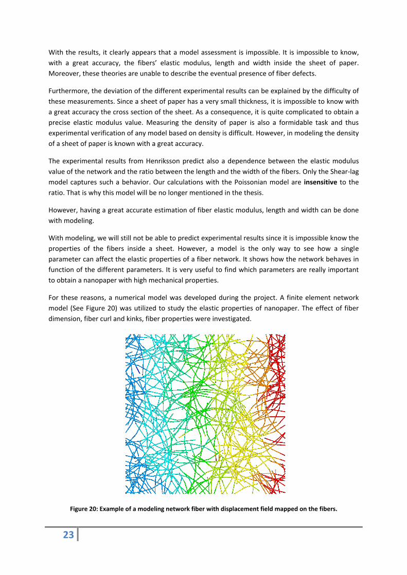
For these reasons, a numerical model was developed during the project. A finite element network

model (See Figure 20) was utilized to study the elastic properties of nanopaper. The effect of fiber

dimension, fiber curl and kinks, fiber properties were investigated.

Figure 20: Example of a modeling network fiber with displacement field mapped on the fibers.

24

4. The finite element model

The model, developed during the thesis, is a two dimensional network model using three

dimensional fibers. All the degrees of freedom out of the plane (Uz, Rotx, Roty) are constrained. The

network is two dimensional due to the layered structure of NFC film (See Figure 56 and [6]). Indeed,

only the elastic properties of one layer are needed to have the elastic properties of the film.

The model is an extension of Heyden’s work *26]. One of the limitations of the previous model is the

inability to consider dense networks. Before, the fibers had to share the nodes in the points of

contacts. Unfortunately, increasing the density required very dense mesh to meet this condition.

Previously, a high density network led to numerical problems. At high density, it was possible to find

two fiber segments overlapping; something impossible to handle with Ansys. We solved this

limitation by using a bonded contact formulation to describe the bonds between the fibers. Fibers

are, now, connected in both translational and rotational degrees of freedom in the points of contacts

but do not share a node.

4.1 The network

In this part, we will describe how we proceed to create the network and how we introduced some

defects inside. We will only focus on the geometrical aspect of the network generation.

4.1.1 The fibers

We will start, first, by the basic component of a sheet of paper; the cellulose fiber. We will present

how we designed the fibers and how we curled them.

4.1.1.1 The geometry

Figure 21: Type of beam used in the model.

The geometry of the fibers is presented in Figure 21. We chose to describe the fibers with square

beam for two reasons. The first one is to have a direct conversion between a two-dimensional

density (our network) and a three-dimensional density (the reality), as defined previously (See

“Comparing the results” p.21). The other advantage to have a square beam is to decrease the

computation time compared to cylindrical beams. Since a beam is a line element, it is only meshed

along the line. So, the cross-section does not affect the number of degrees of freedom. However, the

integration, to visualize the stresses on the deformed shape, is done for the volume and one needs

more integration points to represent a smooth circle compare to a rectangle.

25

We also considered to have an isotropic material with an elastic modulus (Ef) and a Poison ratio (ʋf).

Thus, the shear modulus of the fiber is given directly by )1(2 f

f

f

EG

.

In our network, the classical Euler-Bernoulli’s beam theory is always satisfied. That means 10f

f

W

L.

These fibers are meshed with the 3-node Timoshenko beam elements because these elements are

able to handle a large range of the aspect ratio, and they are free from shear-locking [30].

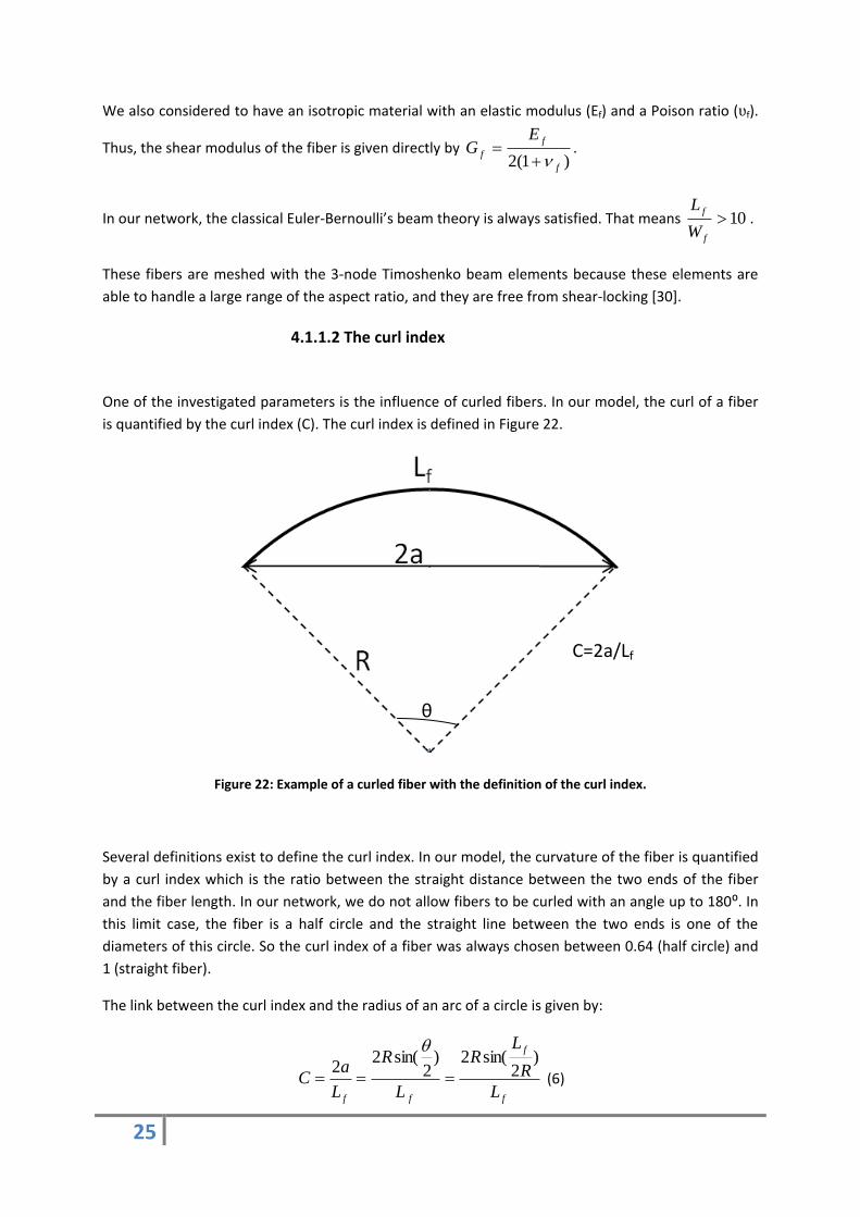
4.1.1.2 The curl index

One of the investigated parameters is the influence of curled fibers. In our model, the curl of a fiber

is quantified by the curl index (C). The curl index is defined in Figure 22.

Figure 22: Example of a curled fiber with the definition of the curl index.

Several definitions exist to define the curl index. In our model, the curvature of the fiber is quantified

by a curl index which is the ratio between the straight distance between the two ends of the fiber

and the fiber length. In our network, we do not allow fibers to be curled with an angle up to 180:. In

this limit case, the fiber is a half circle and the straight line between the two ends is one of the

diameters of this circle. So the curl index of a fiber was always chosen between 0.64 (half circle) and

1 (straight fiber).

The link between the curl index and the radius of an arc of a circle is given by:

f

f

ff L

R

LR

L

R

L

aC

)2

sin(2)2

sin(22

(6)

C=2a/Lf

θ

26

The mathematical relation (5) allows us to design curled fibers in Ansys. Indeed, the radius of

curvature was needed to draw curled fibers. Since the length is known for each fiber, the radius of

curvature can be calculated with the help of the previous relation. Unfortunately, it is impossible to

solve this equation analytically. Different radius values can return the same curl index due to the

periodicity of the sinus function. That is why, we use a graphical representation to determine the

radius of curvature.

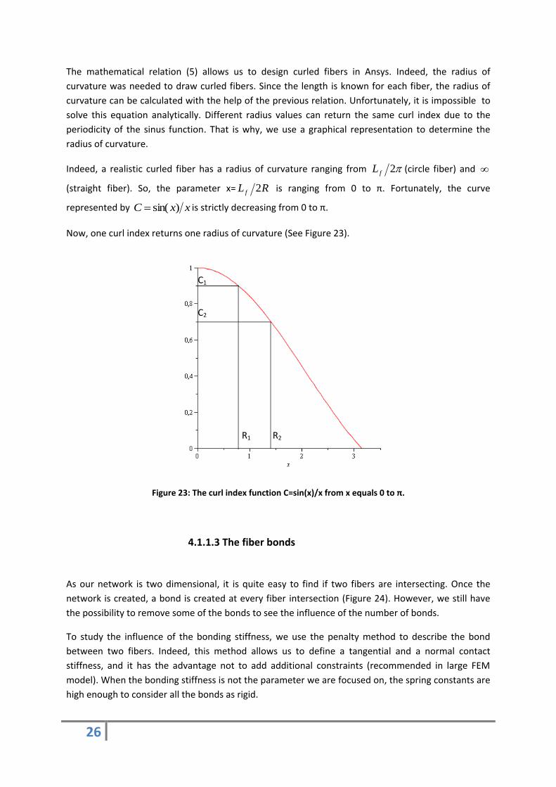
Indeed, a realistic curled fiber has a radius of curvature ranging from 2fL (circle fiber) and

(straight fiber). So, the parameter x= RL f 2 is ranging from 0 to π. Fortunately, the curve

represented by xxC )sin( is strictly decreasing from 0 to π.

Now, one curl index returns one radius of curvature (See Figure 23).

Figure 23: The curl index function C=sin(x)/x from x equals 0 to π.

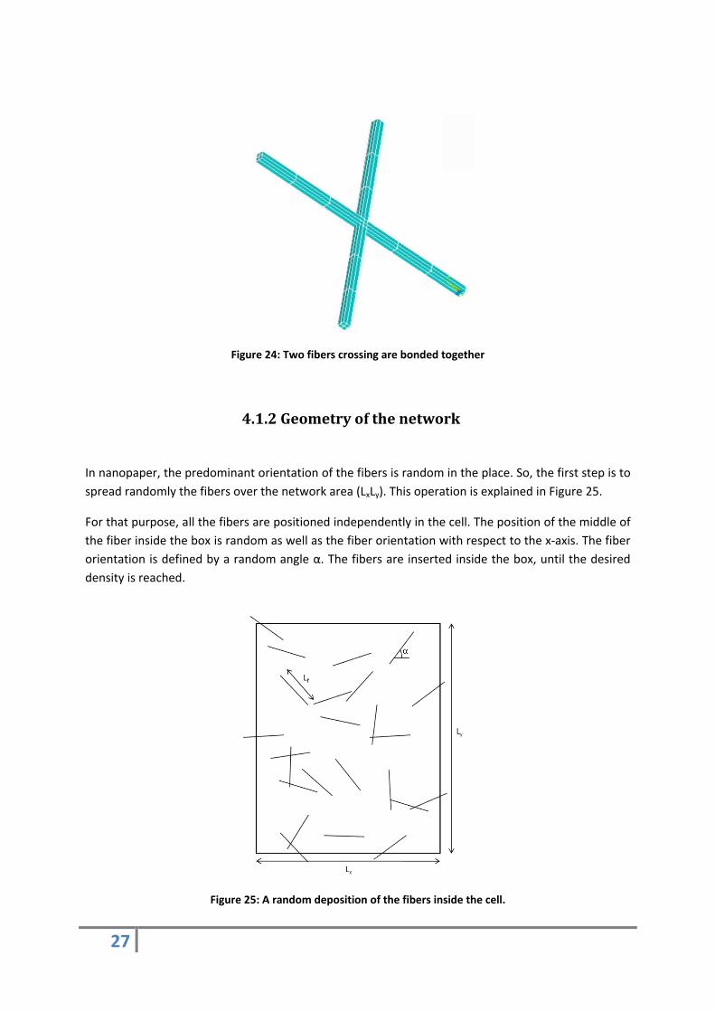
4.1.1.3 The fiber bonds

As our network is two dimensional, it is quite easy to find if two fibers are intersecting. Once the

network is created, a bond is created at every fiber intersection (Figure 24). However, we still have

the possibility to remove some of the bonds to see the influence of the number of bonds.

To study the influence of the bonding stiffness, we use the penalty method to describe the bond

between two fibers. Indeed, this method allows us to define a tangential and a normal contact

stiffness, and it has the advantage not to add additional constraints (recommended in large FEM

model). When the bonding stiffness is not the parameter we are focused on, the spring constants are

high enough to consider all the bonds as rigid.

C1

R1

C2

R2

27

Figure 24: Two fibers crossing are bonded together

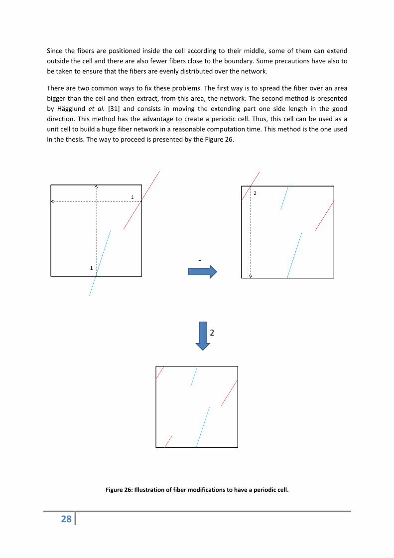
4.1.2 Geometry of the network

In nanopaper, the predominant orientation of the fibers is random in the place. So, the first step is to

spread randomly the fibers over the network area (LxLy). This operation is explained in Figure 25.

For that purpose, all the fibers are positioned independently in the cell. The position of the middle of

the fiber inside the box is random as well as the fiber orientation with respect to the x-axis. The fiber

orientation is defined by a random angle α. The fibers are inserted inside the box, until the desired

density is reached.

Figure 25: A random deposition of the fibers inside the cell.

28

Since the fibers are positioned inside the cell according to their middle, some of them can extend

outside the cell and there are also fewer fibers close to the boundary. Some precautions have also to

be taken to ensure that the fibers are evenly distributed over the network.

There are two common ways to fix these problems. The first way is to spread the fiber over an area

bigger than the cell and then extract, from this area, the network. The second method is presented

by Hägglund et al. [31] and consists in moving the extending part one side length in the good

direction. This method has the advantage to create a periodic cell. Thus, this cell can be used as a

unit cell to build a huge fiber network in a reasonable computation time. This method is the one used

in the thesis. The way to proceed is presented by the Figure 26.

Figure 26: Illustration of fiber modifications to have a periodic cell.

2

1

29

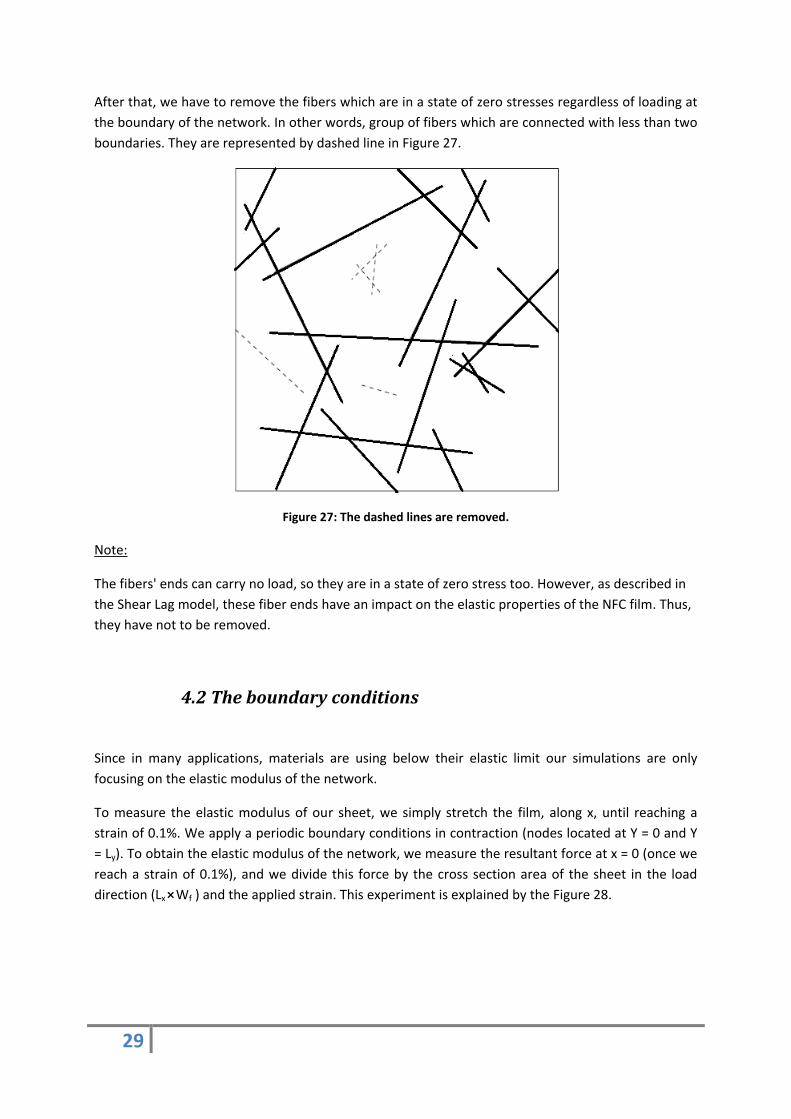
After that, we have to remove the fibers which are in a state of zero stresses regardless of loading at

the boundary of the network. In other words, group of fibers which are connected with less than two

boundaries. They are represented by dashed line in Figure 27.

Figure 27: The dashed lines are removed.

Note:

The fibers' ends can carry no load, so they are in a state of zero stress too. However, as described in

the Shear Lag model, these fiber ends have an impact on the elastic properties of the NFC film. Thus,

they have not to be removed.

4.2 The boundary conditions

Since in many applications, materials are using below their elastic limit our simulations are only

focusing on the elastic modulus of the network.

To measure the elastic modulus of our sheet, we simply stretch the film, along x, until reaching a

strain of 0.1%. We apply a periodic boundary conditions in contraction (nodes located at Y = 0 and Y

= Ly). To obtain the elastic modulus of the network, we measure the resultant force at x = 0 (once we

reach a strain of 0.1%), and we divide this force by the cross section area of the sheet in the load

direction (Lx⨯Wf ) and the applied strain. This experiment is explained by the Figure 28.

30

Figure 28: Boundary conditions applied to the network.

4.3 Convergence

Before starting the analysis of the results, we have to take care about the convergence of our results

(a stable elastic modulus value). In your case two different situations have to be taken into account,

the number of elements per fibers (also called “the meshing convergence”) and the size of the

network (also called the “geometrical convergence”).

4.3.1 The meshing convergence

In all numerical analyses, when comes to mesh the system, there is always a dilemma between the

precision of the results and the computation time. If a FEM analysis is done correctly, a finer mesh

will return more precise results (in some simple cases, it will return the same results), but it will also

increase the computation time. The dilemma is to have an acceptable precision in a reasonable time.

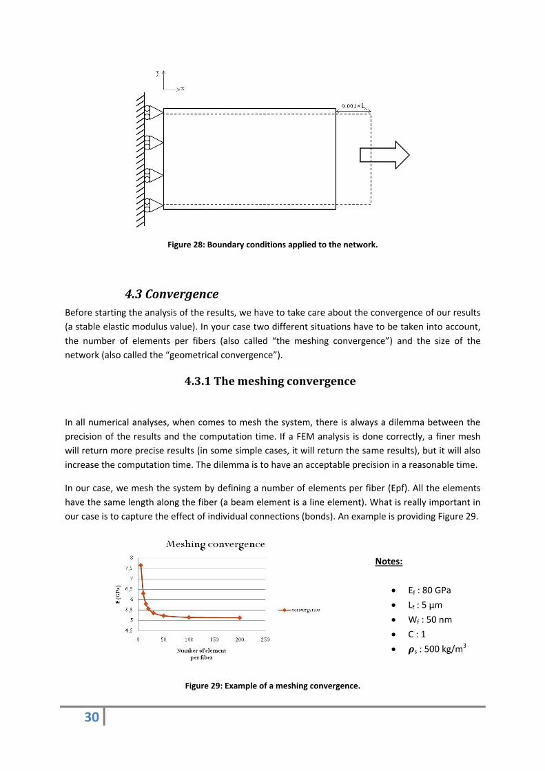
In our case, we mesh the system by defining a number of elements per fiber (Epf). All the elements

have the same length along the fiber (a beam element is a line element). What is really important in

our case is to capture the effect of individual connections (bonds). An example is providing Figure 29.

Notes:

Ef : 80 GPa

Lf : 5 μm

Wf : 50 nm

C : 1

s : 500 kg/m3

Figure 29: Example of a meshing convergence.

31

In the example below, at least 30 elements per fiber are necessary to have a relative error on the

elastic modulus value lower than 5%. However, the numbers of elements per fiber have to increase

when the density increased or when the ratio between the length and the width of the fiber increase

(for the same network). Indeed, in both cases, the number of contact (bonds) per fiber increases,

thus a finer mesh is required to capture the effect of each connection.

Unfortunately, a higher density or a higher ratio increases the number of fiber inside the network.

Thus the number of elements inside the network increases without changing the number of element

per fiber. To avoid memory problem and very long time computation, the number of density per

fiber is kept, most of the time, at 50 elements per fiber.

4.3.2 The size convergence

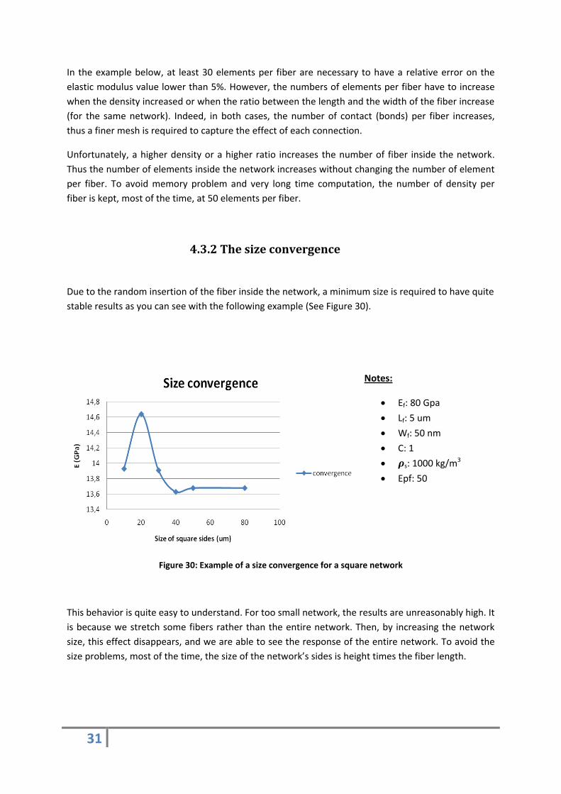
Due to the random insertion of the fiber inside the network, a minimum size is required to have quite

stable results as you can see with the following example (See Figure 30).

Notes:

Ef: 80 Gpa

Lf: 5 um

Wf: 50 nm

C: 1

s: 1000 kg/m3

Epf: 50

Figure 30: Example of a size convergence for a square network

This behavior is quite easy to understand. For too small network, the results are unreasonably high. It

is because we stretch some fibers rather than the entire network. Then, by increasing the network

size, this effect disappears, and we are able to see the response of the entire network. To avoid the

size problems, most of the time, the size of the network’s sides is height times the fiber length.

32

The meshing convergence combined with the size convergence can lead to a network with more than

5 800 000 elements (34 millions degree of freedom). This ability to compute such a dense network is

a great advance of our model. The previous models were unable to compute such network due to

numerical problems such as elements overlapping and memory problems. We are now able to study

the effect of very dense network, which is closer to experimental measurements (See “The

experimental results” p.52 and Figure 31).

Figure 31: Picture of a Bacteria cellulose sheet; a very dense network.

33

5. The Results

With our model, we tried to understand the effects of several parameters on the global stiffness of

the network. As mentioned previously, only the elastic properties were investigated since most of

the industrial applications required materials working below the plastic regime. This chapter will

present all our observations and results.

5.1 An homogeneous network

A fiber network is a quite complex system. The mean field theory (MFT) is often used to solve

mechanical problems dealing with fiber network. The main idea of MFT is to assume that the

interaction of one constituent (on the global system) is the average interaction of its neighboring

constituents. This reduces any multi-body problem into an effective one-body problem. Thus, the

behavior of the system can be obtained at a relatively low cost. All the theoretical models assumed

that this theory is available in case of fiber networks.

However, the mean field theory can be only applied in case of a homogenous system.

By mapping the displacement field (see Figure 32) and the equivalent stress field (see Figure 33) over

the fibers, one can see that the mean field theory can be well applied to this particular type of

structure. Indeed, we obtained continuous displacement field and, thus, a homogenous stress field.

Notes:

Ef: 80 Gpa

Lf: 5 um

Wf: 50 nm

C: random

s: 1000 kg/m3

Epf: 50

Figure 32: A homogeneous displacement field.

34

Notes:

Ef: 80 Gpa

Lf: 5 um

Wf: 50 nm

C: random

s: 1000 kg/m3

Epf: 50

Figure 33: A homogeneous stress field.

5.2 Effect of the density

All the previous theoretical models and empirical observations assume a linear dependence between

the density of a network and the elastic modulus of the network. Our model shows exactly this

behavior (See Figure 34). This good agreement between our model and the previous study shows the

reliability of our model.

So, one of the first things to increase the elastic modulus of the paper is to increase the density of

the sheet. However, scientists are now able to produce nanopaper with very high density (porosity

lower than 20%). Thus the density is not the main point to focus on to increase the elastic properties.

So, why are the predictions so high compare to the experimental results?

Notes:

Ef: 80 Gpa

Lf: 5 um

Wf: 50 nm

C: 1

Epf: 50

Figure 34: The influence of the density on the elastic modulus of a fiber network

35

5.3 Dimensions of the fibers

According to the results obtained by Marielle Henriksson et al., we supposed an influence of the

dimensions of the fibers on the global elastic properties of the cellulose fibers' network.

The Shear-lag theory also shows a strong dependence between the dimensions of the fibers (more

precisely the ratio between the length and the width) and the elastic modulus since the K constant

and the percolation density will change function of the ratio (See Equation 3).

The simulations are in accordance to the Shear-lag theory, is that only the ratio of the fiber length to

the width is important. However, this ratio has a strong effect on the elastic modulus (See Figure 35).

By multiplying the ratio (length to the width) by two (from 100 to 200), our model shows an increase

of approximately 3 GPa.

This dependence can be explained by the total length of fiber ends. The lower is the ratio of the fiber

length to the width, the larger is the total length of fiber ends. Since the fiber ends can carry no load,

by increasing the total length of fiber ends, the elastic modulus of the network decrease. This is

responsible for the influence of the ratio.

Notes:

Ef: 80 Gpa

C: 1

Epf: 50

Figure 35: The influence of the density on the elastic modulus of a fiber network

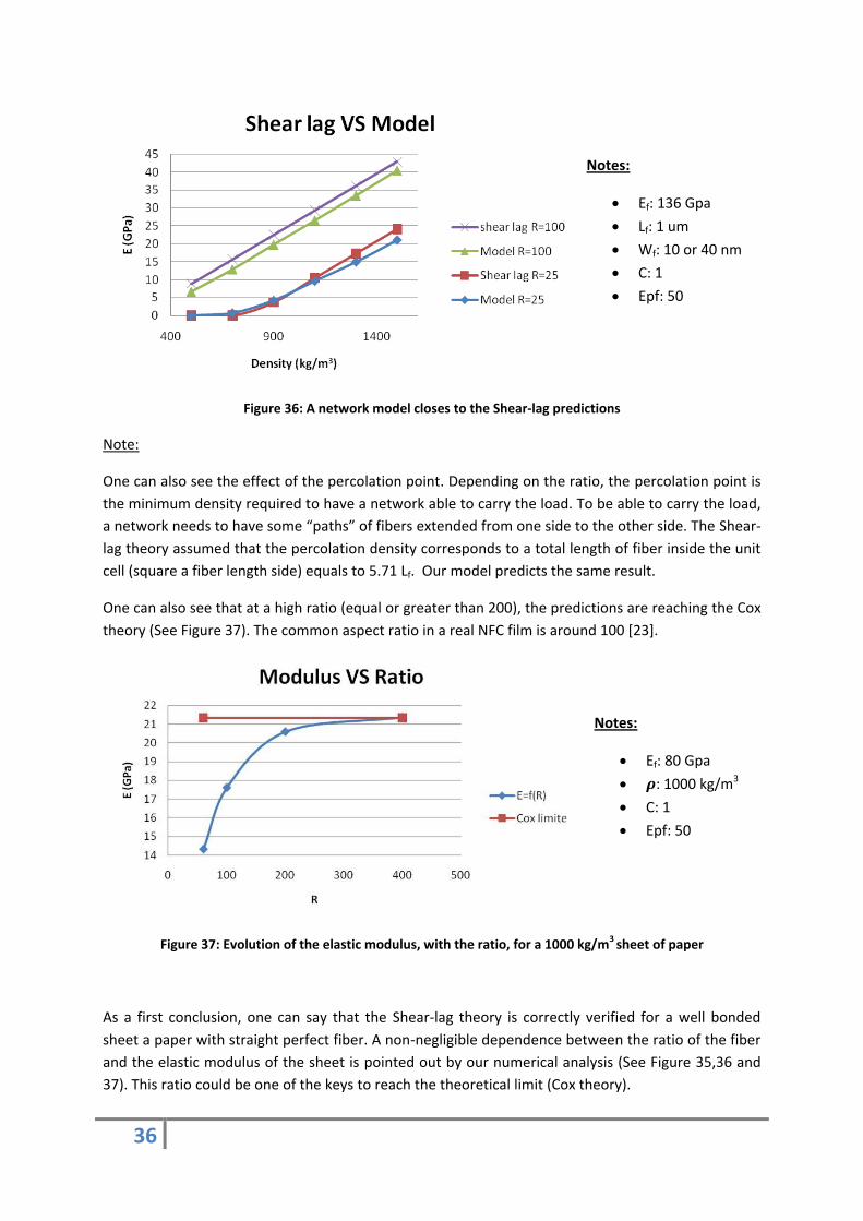
As enounced previously, the Shear-lag theory predicts an influence of the ratio of the fiber length to

the fiber width (See “The Shear-lag model” p.18). So, we compared the theoretical results with our

model. The numerical results we obtained for two “Shear-lag” networks (a network with straight

fibers rigidly bonded together), having fibers with a different aspect ratio, were close to the

theoretical predictions (See Figure 36).

There is still a slight difference in the modulus value. There are several reasons which can explain the

lower values of our model. In our model, the fibers are allowed to deform into bending deformation

and the poisson contraction of the fibers is taken into account. Of course, this is not the case in the

Shear-lag theory. This theory assumes also that the fibers are the unit of the network and the

calculus are based on a stress variation along the fiber. In reality, the basic unit of the network is the

segment between two fiber bonds.

36

Notes:

Ef: 136 Gpa

Lf: 1 um

Wf: 10 or 40 nm

C: 1

Epf: 50

Figure 36: A network model closes to the Shear-lag predictions

Note:

One can also see the effect of the percolation point. Depending on the ratio, the percolation point is

the minimum density required to have a network able to carry the load. To be able to carry the load,

a network needs to have some “paths” of fibers extended from one side to the other side. The Shear-

lag theory assumed that the percolation density corresponds to a total length of fiber inside the unit

cell (square a fiber length side) equals to 5.71 Lf. Our model predicts the same result.

One can also see that at a high ratio (equal or greater than 200), the predictions are reaching the Cox

theory (See Figure 37). The common aspect ratio in a real NFC film is around 100 [23].

Notes:

Ef: 80 Gpa

: 1000 kg/m3

C: 1

Epf: 50

Figure 37: Evolution of the elastic modulus, with the ratio, for a 1000 kg/m3 sheet of paper

As a first conclusion, one can say that the Shear-lag theory is correctly verified for a well bonded

sheet a paper with straight perfect fiber. A non-negligible dependence between the ratio of the fiber

and the elastic modulus of the sheet is pointed out by our numerical analysis (See Figure 35,36 and

37). This ratio could be one of the keys to reach the theoretical limit (Cox theory).

37

5.4 Influence of curled fibers and bonds

In some ways, the model is quite far from the reality. First of all, inside a sheet of paper (ordinary

paper and nanopaper), the fibers’ network is three dimensional. The fibers may not be rigidly bonded

as we assumed in our previous experiment, and they cannot be considered as straight. In this part,

we will add more realistic parameters to our model and see the influence of them on the elastic

modulus.

5.4.1 The influence of the bonds

The influence of the bonds can be separated into two different parameters: the bond activation and

the bond contact stiffness. A bond is active when two fibers crossing each other are physically or

chemically linked together (a stress transfer is able between the two fibers). On the contrary, a fiber

bond is non active when there is no interaction between two fibers crossing.

The bond activation was investigated because, in our two dimensional model, an active bond is

created when two fibers are crossing in the plan. However, in a real NFC film, the network is three

dimensional. Thus, two fibers crossing in the plan (x, y) may be separate by a non-negligible distance

along the z-axis, preventing them to form a bond. Moreover, in NFC films, the presence of water

creates strong hydrogen interactions between the fibers. These interactions are mainly responsible

for the bonds’ activation (formation of hydrogen bonds). However, a lack of hydrogen interactions

due to a lack of water or the use of a non polar solvent can prevent the formation of some bonds.

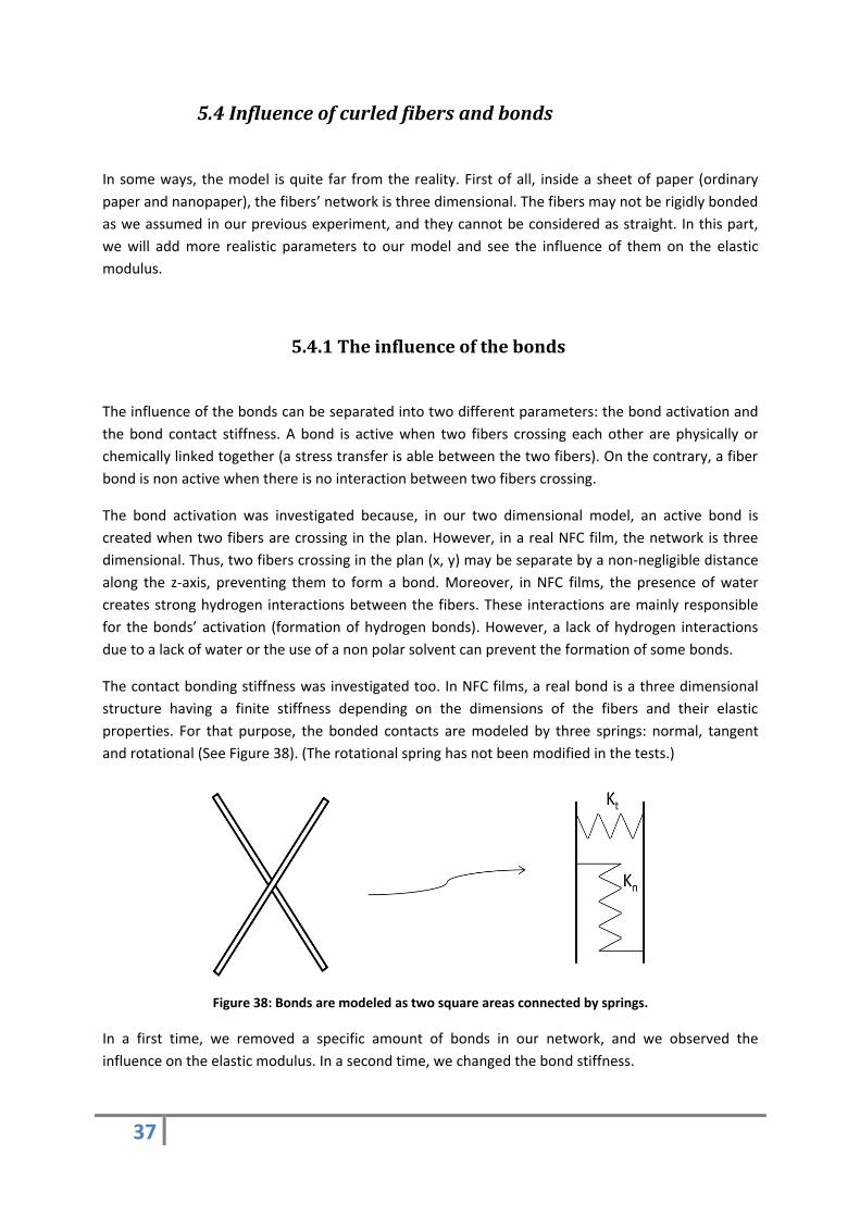
The contact bonding stiffness was investigated too. In NFC films, a real bond is a three dimensional

structure having a finite stiffness depending on the dimensions of the fibers and their elastic

properties. For that purpose, the bonded contacts are modeled by three springs: normal, tangent

and rotational (See Figure 38). (The rotational spring has not been modified in the tests.)

Figure 38: Bonds are modeled as two square areas connected by springs.

In a first time, we removed a specific amount of bonds in our network, and we observed the

influence on the elastic modulus. In a second time, we changed the bond stiffness.

38

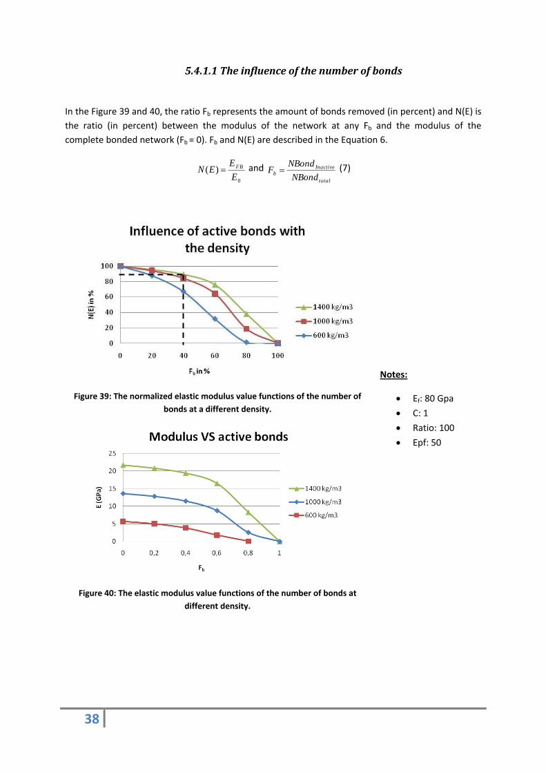
5.4.1.1 The influence of the number of bonds

In the Figure 39 and 40, the ratio Fb represents the amount of bonds removed (in percent) and N(E) is

the ratio (in percent) between the modulus of the network at any Fb and the modulus of the

complete bonded network (Fb = 0). Fb and N(E) are described in the Equation 6.

0

)(E

EEN FB and

total

Inactive

bNBond

NBondF (7)

Figure 39: The normalized elastic modulus value functions of the number of

bonds at a different density.

Notes:

Ef: 80 Gpa

C: 1

Ratio: 100

Epf: 50

Figure 40: The elastic modulus value functions of the number of bonds at

different density.

39

With the Figure 39 and 40, it appears that the modulus of the network is quite stable in the range of

density usually measured for cellulose nanopaper (around 1200 kg/m3 [6]). Indeed, to decrease the

elastic modulus of the network by 10%, at least 40% of the bonds has to be removed. However, the

bond’s activation influences the stiffness of sparser network (around 600 kg/m3).

According to these measurements and our results, the number of bonds to remove, to reduce the

elastic modulus by 10% is too large to be realistic. Thus, the number of bond (or bond activation) is

not a parameter which can explain the large difference between the experimental measurements

and the theoretical values predicted by Cox.

5.4.1.2 The influence of bonding stiffness

The phenomenon of fiber-fiber interaction is composed by several mechanisms acting together. For

example, kinked fibers can honk onto each other. Other phenomenons such as fiber-to-fiber friction

and hydrogen interactions have to be taken into account too. So, in a real sheet of nanopaper, fiber

to fiber interaction is a complex phenomenon. That is why, it is quite impossible to know,

experimentally, the real bonding stiffness value. We estimated the bonding stiffness in a real

nanopaper to be only dependent on the elastic properties of the fibers and the dimensions of the

bonds. It leads us to:

(8)

However, cellulose nanofibers are not isotropic and exhibit a transversal elastic modulus around

20 GPa [32]. Since, the bond stiffness is dependent on the transversal elastic properties of the fiber,

we divided the previous stiffness (See Equation 8) by ten to get more realistic. In other words, we

assumed to have a transversal modulus of the fibers equal to Ef/10. Indeed, Ef represents the normal

elastic modulus of the fibers and is around 140 GPa.

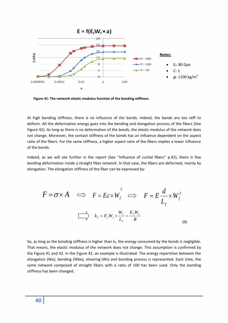
At the next step, several elastic modulus measurements are done on our network with a different

bonding stiffness and different ratio of fiber. The obtained results are presented in Figure 41 where

the elastic modulus of the network is represented function of the bonding stiffness.

AF 2

fWEF 2

f

f

WW

dEF

fftn WEkk

40

Figure 41: The network elastic modulus function of the bonding stiffness.

Notes:

Ef: 80 Gpa

C: 1

: 1100 kg/m3

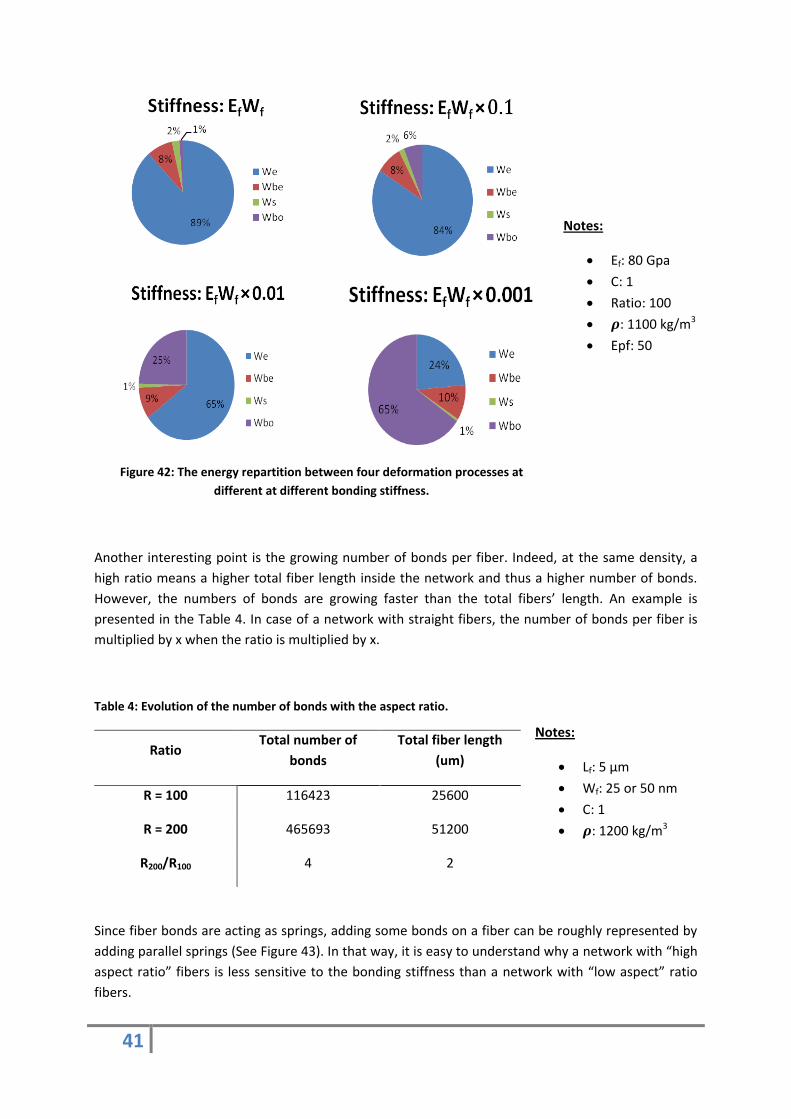
At high bonding stiffness, there is no influence of the bonds. Indeed, the bonds are too stiff to

deform. All the deformation energy goes into the bending and elongation process of the fibers (See

Figure 42). As long as there is no deformation of the bonds, the elastic modulus of the network does

not change. Moreover, the contact stiffness of the bonds has an influence dependent on the aspect

ratio of the fibers. For the same stiffness, a higher aspect ratio of the fibers implies a lower influence

of the bonds.

Indeed, as we will see further in the report (See “Influence of curled fibers” p.42), there is few

bending deformation inside a straight fiber network. In that case, the fibers are deformed, mainly by

elongation. The elongation stiffness of the fiber can be expressed by:

(9)

So, as long as the bonding stiffness is higher than kf, the energy consumed by the bonds is negligible.

That means, the elastic modulus of the network does not change. This assumption is confirmed by

the Figure 41 and 42. In the Figure 42, an example is illustrated. The energy repartition between the

elongation (We), bending (Wbe), shearing (Ws) and bonding process is represented. Each time, the

same network composed of straight fibers with a ratio of 100 has been used. Only the bonding

stiffness has been changed.

AF 2

fWEF 2

f

f

WL

dEF

R

WE

L

WWEk

ff

f

f

fff

41

Notes:

Ef: 80 Gpa

C: 1

Ratio: 100

: 1100 kg/m3

Epf: 50

Figure 42: The energy repartition between four deformation processes at

different at different bonding stiffness.

Another interesting point is the growing number of bonds per fiber. Indeed, at the same density, a

high ratio means a higher total fiber length inside the network and thus a higher number of bonds.

However, the numbers of bonds are growing faster than the total fibers’ length. An example is

presented in the Table 4. In case of a network with straight fibers, the number of bonds per fiber is

multiplied by x when the ratio is multiplied by x.

Table 4: Evolution of the number of bonds with the aspect ratio.

Ratio Total number of

bonds

Total fiber length

(um)

R = 100 116423 25600

R = 200 465693 51200

R200/R100 4 2

Notes:

Lf: 5 μm

Wf: 25 or 50 nm

C: 1

: 1200 kg/m3

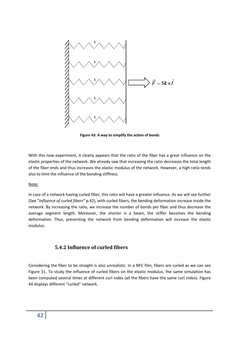
Since fiber bonds are acting as springs, adding some bonds on a fiber can be roughly represented by

adding parallel springs (See Figure 43). In that way, it is easy to understand why a network with “high

aspect ratio” fibers is less sensitive to the bonding stiffness than a network with “low aspect” ratio

fibers.

42

Figure 43: A way to simplify the action of bonds

With this new experiment, it clearly appears that the ratio of the fiber has a great influence on the

elastic properties of the network. We already saw that increasing the ratio decreases the total length

of the fiber ends and thus increases the elastic modulus of the network. However, a high ratio tends

also to limit the influence of the bonding stiffness.

Note:

In case of a network having curled fiber, this ratio will have a greater influence. As we will see further

(See ”Influence of curled fibers” p.42), with curled fibers, the bending deformation increase inside the

network. By increasing the ratio, we increase the number of bonds per fiber and thus decrease the

average segment length. Moreover, the shorter is a beam, the stiffer becomes the bending

deformation. Thus, preventing the network from bending deformation will increase the elastic

modulus.

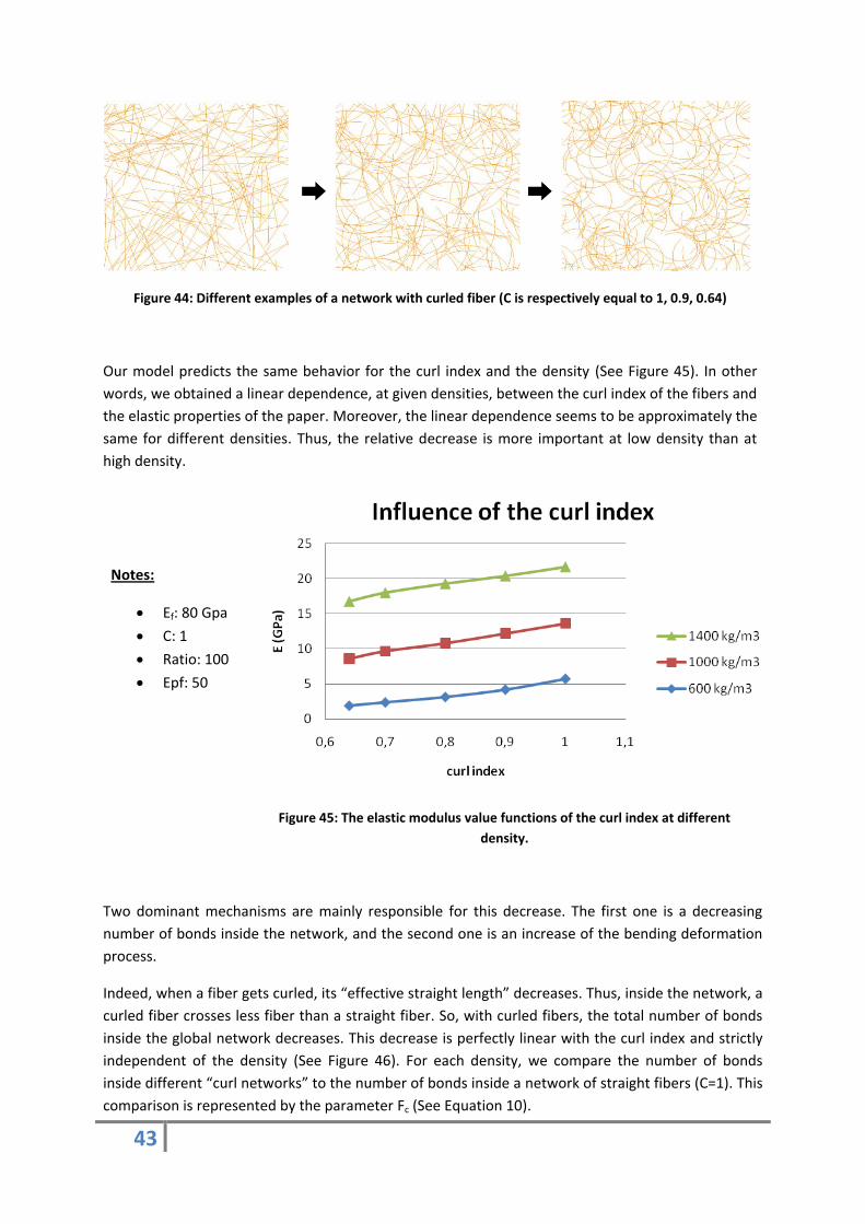
5.4.2 Influence of curled fibers

Considering the fiber to be straight is also unrealistic. In a NFC film, fibers are curled as we can see

Figure 31. To study the influence of curled fibers on the elastic modulus, the same simulation has

been computed several times at different curl index (all the fibers have the same curl index). Figure

44 displays different “curled” network.

43

Figure 44: Different examples of a network with curled fiber (C is respectively equal to 1, 0.9, 0.64)

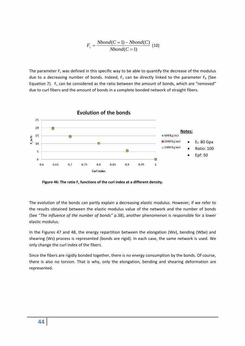
Our model predicts the same behavior for the curl index and the density (See Figure 45). In other

words, we obtained a linear dependence, at given densities, between the curl index of the fibers and

the elastic properties of the paper. Moreover, the linear dependence seems to be approximately the

same for different densities. Thus, the relative decrease is more important at low density than at

high density.

Notes:

Ef: 80 Gpa

C: 1

Ratio: 100

Epf: 50

Figure 45: The elastic modulus value functions of the curl index at different

density.

Two dominant mechanisms are mainly responsible for this decrease. The first one is a decreasing

number of bonds inside the network, and the second one is an increase of the bending deformation

process.

Indeed, when a fiber gets curled, its “effective straight length” decreases. Thus, inside the network, a

curled fiber crosses less fiber than a straight fiber. So, with curled fibers, the total number of bonds

inside the global network decreases. This decrease is perfectly linear with the curl index and strictly

independent of the density (See Figure 46). For each density, we compare the number of bonds

inside different “curl networks” to the number of bonds inside a network of straight fibers (C=1). This

comparison is represented by the parameter Fc (See Equation 10).

44

)1(

)()1(

CNbond

CNbondCNbondFc (10)

The parameter Fc was defined in this specific way to be able to quantify the decrease of the modulus

due to a decreasing number of bonds. Indeed, Fc can be directly linked to the parameter Fb (See

Equation 7). Fc can be considered as the ratio between the amount of bonds, which are “removed”

due to curl fibers and the amount of bonds in a complete bonded network of straight fibers.

Figure 46: The ratio Fc functions of the curl index at a different density.

Notes:

Ef: 80 Gpa

Ratio: 100

Epf: 50

The evolution of the bonds can partly explain a decreasing elastic modulus. However, if we refer to

the results obtained between the elastic modulus value of the network and the number of bonds

(See “The influence of the number of bonds” p.38), another phenomenon is responsible for a lower

elastic modulus.

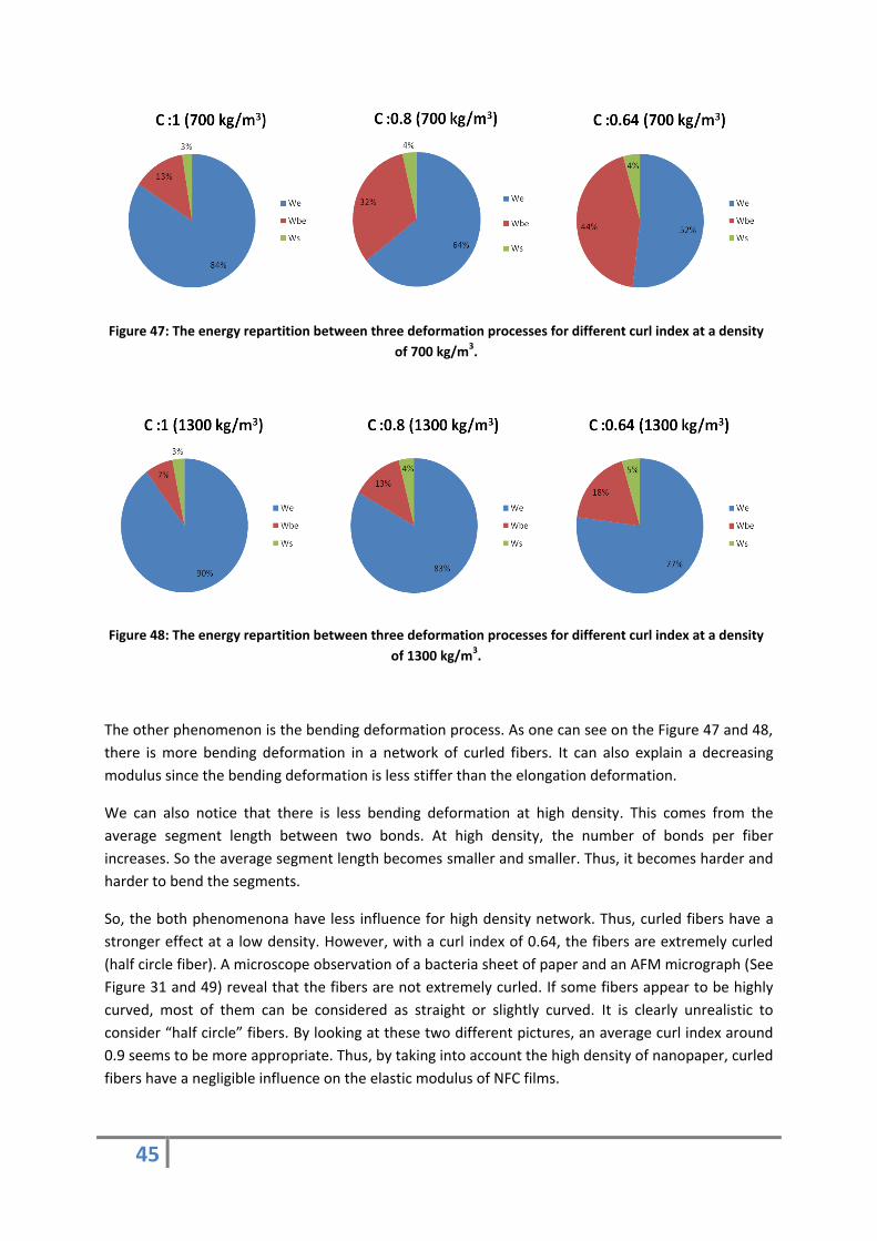
In the Figures 47 and 48, the energy repartition between the elongation (We), bending (Wbe) and

shearing (Ws) process is represented (bonds are rigid). In each case, the same network is used. We

only change the curl index of the fibers.

Since the fibers are rigidly bonded together, there is no energy consumption by the bonds. Of course,

there is also no torsion. That is why, only the elongation, bending and shearing deformation are

represented.

45

Figure 47: The energy repartition between three deformation processes for different curl index at a density

of 700 kg/m3.

Figure 48: The energy repartition between three deformation processes for different curl index at a density

of 1300 kg/m3.

The other phenomenon is the bending deformation process. As one can see on the Figure 47 and 48,

there is more bending deformation in a network of curled fibers. It can also explain a decreasing

modulus since the bending deformation is less stiffer than the elongation deformation.

We can also notice that there is less bending deformation at high density. This comes from the

average segment length between two bonds. At high density, the number of bonds per fiber

increases. So the average segment length becomes smaller and smaller. Thus, it becomes harder and

harder to bend the segments.

So, the both phenomenona have less influence for high density network. Thus, curled fibers have a

stronger effect at a low density. However, with a curl index of 0.64, the fibers are extremely curled

(half circle fiber). A microscope observation of a bacteria sheet of paper and an AFM micrograph (See

Figure 31 and 49) reveal that the fibers are not extremely curled. If some fibers appear to be highly

curved, most of them can be considered as straight or slightly curved. It is clearly unrealistic to

consider “half circle” fibers. By looking at these two different pictures, an average curl index around

0.9 seems to be more appropriate. Thus, by taking into account the high density of nanopaper, curled

fibers have a negligible influence on the elastic modulus of NFC films.

46

Figure 49: AFM micrograph of a “wood cellulose” nanopaper.

However, the bonding stiffness can decrease dramatically the global elastic modulus of the network,

and its effect seems to be directly linked to the ratio of the fiber. Unfortunately, the “bond

mechanism” is a quite complex phenomenon, not very well understand. Thus, it seems quite difficult

to estimate the real bonding stiffness inside a NFC film. However, our simulations show another

time, the great influence of the ratio of the fibers. Contrary to the other parameters such as the curl

fibers and the bond activation, the aspect ratio of the fibers shows a great influence on the elastic

properties of the network.

47

6. Experimental section

At the end of the project, several experiments were done to compare the simulations and the reality.

These experiments were focused on the ratio of the fibers and the elastic modulus of the NFC films,

since the ratio is the parameters with the strongest influence in our numerical model. For that

purpose, two NFC films with different fibers were manufactured. Their respective elastic properties

were investigated using tensile tests, and a scanning electron microscope (SEM) was used to observe

the nanofibrils. Several mechanical tests on a common printing paper have been performed too.

Due to a lack of time, this experimental analysis cannot be considered as complete, but it gives

interesting results and valuable information to do the experiments in good conditions.

6.1 How to obtain NFC films?

As developed before, two different ways exist to obtain NFC. The first one is to break down the plant

structure, and the second one is to use a raw material that already has these structural forms.

Indeed, the cellulose produced by bacteria and tunicates are already in a form a non-woven network

composed by NFC. The big advantages of these methods are to produce ready to use cellulose fiber

networks with non-damaged fibers. The main drawback is the manufacturing time. Unfortunately,

manufacturing a NFC film with bacteria takes approximately four weeks. Due to supplier problems,

we used NFC extracted from wood to product our films.

To obtain NFC from wood, the pulp (See “The pulping process” p.10) has to undergo intensive

mechanical treatments. The manufacture is generally performed by refining and high pressure

homogenizing process steps. The dilute fiber suspension is forced through a gap between a rotor and

a stator disk. Here, the fibers are subjected to repeated high shear stress (See Figure 50). This

process leads to the nanofibrillation of the fibers. This step of the process was done at the company

Innventia, Stockholm, Sweden.

Figure 50: Obtaining NFC with wood pulp.

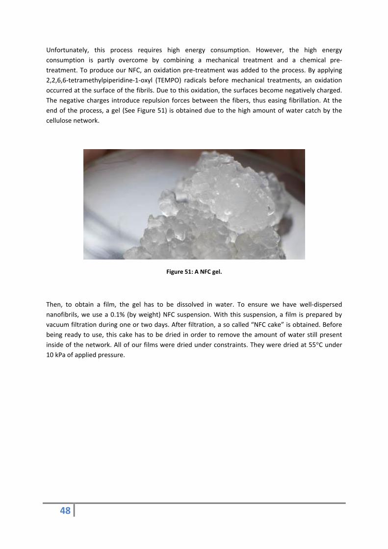
48

Unfortunately, this process requires high energy consumption. However, the high energy

consumption is partly overcome by combining a mechanical treatment and a chemical pre-

treatment. To produce our NFC, an oxidation pre-treatment was added to the process. By applying

2,2,6,6-tetramethylpiperidine-1-oxyl (TEMPO) radicals before mechanical treatments, an oxidation

occurred at the surface of the fibrils. Due to this oxidation, the surfaces become negatively charged.

The negative charges introduce repulsion forces between the fibers, thus easing fibrillation. At the

end of the process, a gel (See Figure 51) is obtained due to the high amount of water catch by the

cellulose network.

Figure 51: A NFC gel.

Then, to obtain a film, the gel has to be dissolved in water. To ensure we have well-dispersed

nanofibrils, we use a 0.1% (by weight) NFC suspension. With this suspension, a film is prepared by

vacuum filtration during one or two days. After filtration, a so called “NFC cake” is obtained. Before

being ready to use, this cake has to be dried in order to remove the amount of water still present

inside of the network. All of our films were dried under constraints. They were dried at 55°C under

10 kPa of applied pressure.

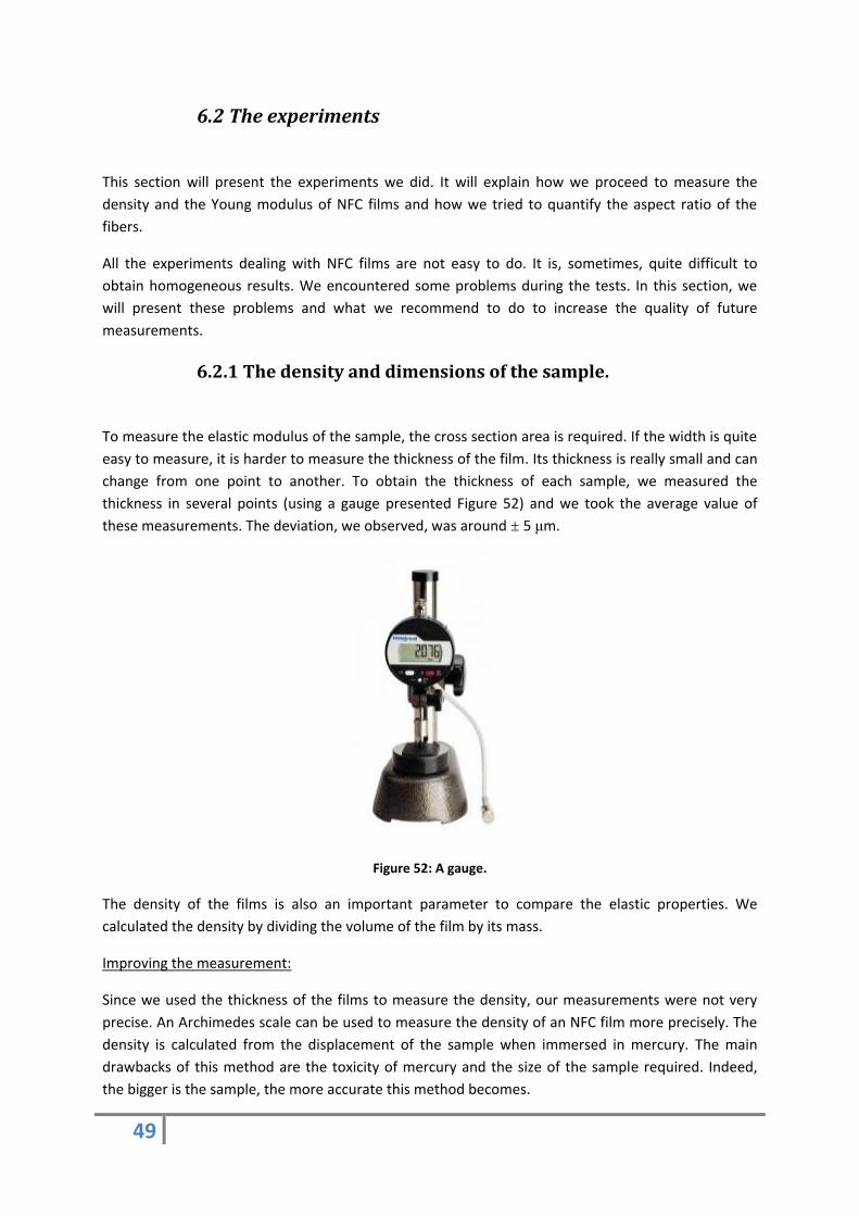
49

6.2 The experiments

This section will present the experiments we did. It will explain how we proceed to measure the

density and the Young modulus of NFC films and how we tried to quantify the aspect ratio of the

fibers.

All the experiments dealing with NFC films are not easy to do. It is, sometimes, quite difficult to

obtain homogeneous results. We encountered some problems during the tests. In this section, we

will present these problems and what we recommend to do to increase the quality of future

measurements.

6.2.1 The density and dimensions of the sample.

To measure the elastic modulus of the sample, the cross section area is required. If the width is quite

easy to measure, it is harder to measure the thickness of the film. Its thickness is really small and can

change from one point to another. To obtain the thickness of each sample, we measured the

thickness in several points (using a gauge presented Figure 52) and we took the average value of

these measurements. The deviation, we observed, was around ± 5 μm.

Figure 52: A gauge.

The density of the films is also an important parameter to compare the elastic properties. We

calculated the density by dividing the volume of the film by its mass.

Improving the measurement:

Since we used the thickness of the films to measure the density, our measurements were not very

precise. An Archimedes scale can be used to measure the density of an NFC film more precisely. The

density is calculated from the displacement of the sample when immersed in mercury. The main

drawbacks of this method are the toxicity of mercury and the size of the sample required. Indeed,

the bigger is the sample, the more accurate this method becomes.

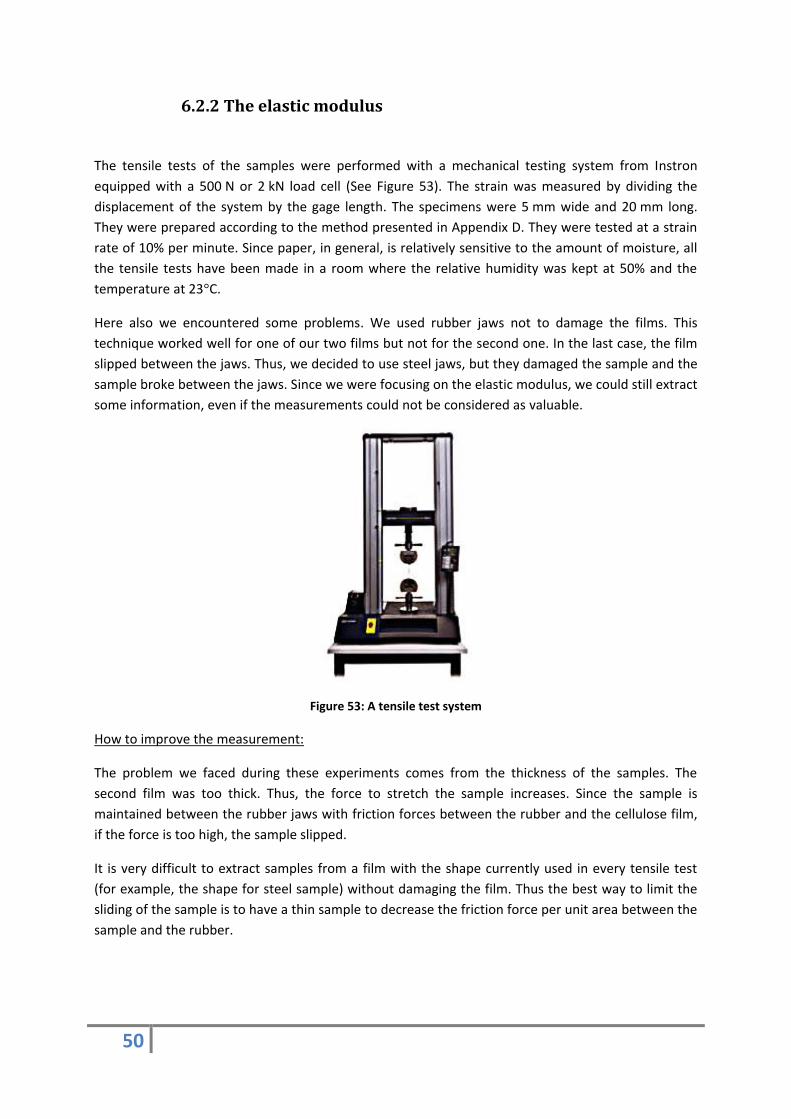
50

6.2.2 The elastic modulus

The tensile tests of the samples were performed with a mechanical testing system from Instron

equipped with a 500 N or 2 kN load cell (See Figure 53). The strain was measured by dividing the

displacement of the system by the gage length. The specimens were 5 mm wide and 20 mm long.

They were prepared according to the method presented in Appendix D. They were tested at a strain

rate of 10% per minute. Since paper, in general, is relatively sensitive to the amount of moisture, all

the tensile tests have been made in a room where the relative humidity was kept at 50% and the

temperature at 23°C.

Here also we encountered some problems. We used rubber jaws not to damage the films. This

technique worked well for one of our two films but not for the second one. In the last case, the film

slipped between the jaws. Thus, we decided to use steel jaws, but they damaged the sample and the

sample broke between the jaws. Since we were focusing on the elastic modulus, we could still extract

some information, even if the measurements could not be considered as valuable.

Figure 53: A tensile test system

How to improve the measurement:

The problem we faced during these experiments comes from the thickness of the samples. The

second film was too thick. Thus, the force to stretch the sample increases. Since the sample is

maintained between the rubber jaws with friction forces between the rubber and the cellulose film,

if the force is too high, the sample slipped.

It is very difficult to extract samples from a film with the shape currently used in every tensile test

(for example, the shape for steel sample) without damaging the film. Thus the best way to limit the

sliding of the sample is to have a thin sample to decrease the friction force per unit area between the

sample and the rubber.

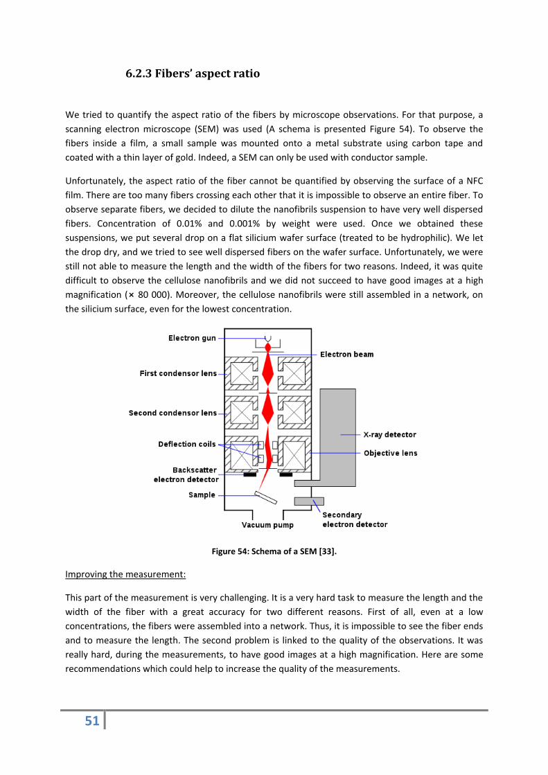
51

6.2.3 Fibers’ aspect ratio

We tried to quantify the aspect ratio of the fibers by microscope observations. For that purpose, a

scanning electron microscope (SEM) was used (A schema is presented Figure 54). To observe the

fibers inside a film, a small sample was mounted onto a metal substrate using carbon tape and

coated with a thin layer of gold. Indeed, a SEM can only be used with conductor sample.

Unfortunately, the aspect ratio of the fiber cannot be quantified by observing the surface of a NFC

film. There are too many fibers crossing each other that it is impossible to observe an entire fiber. To

observe separate fibers, we decided to dilute the nanofibrils suspension to have very well dispersed

fibers. Concentration of 0.01% and 0.001% by weight were used. Once we obtained these

suspensions, we put several drop on a flat silicium wafer surface (treated to be hydrophilic). We let

the drop dry, and we tried to see well dispersed fibers on the wafer surface. Unfortunately, we were

still not able to measure the length and the width of the fibers for two reasons. Indeed, it was quite

difficult to observe the cellulose nanofibrils and we did not succeed to have good images at a high

magnification (⨯ 80 000). Moreover, the cellulose nanofibrils were still assembled in a network, on

the silicium surface, even for the lowest concentration.

Figure 54: Schema of a SEM [33].

Improving the measurement:

This part of the measurement is very challenging. It is a very hard task to measure the length and the

width of the fiber with a great accuracy for two different reasons. First of all, even at a low

concentrations, the fibers were assembled into a network. Thus, it is impossible to see the fiber ends

and to measure the length. The second problem is linked to the quality of the observations. It was

really hard, during the measurements, to have good images at a high magnification. Here are some

recommendations which could help to increase the quality of the measurements.

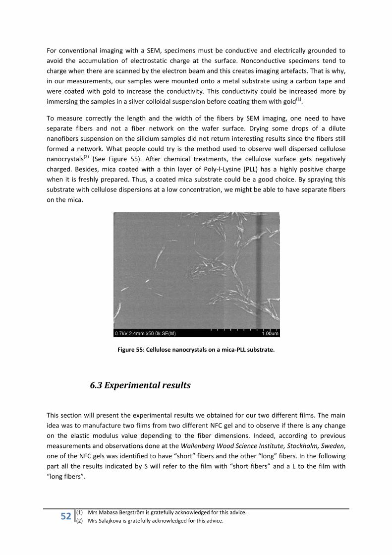
52

For conventional imaging with a SEM, specimens must be conductive and electrically grounded to

avoid the accumulation of electrostatic charge at the surface. Nonconductive specimens tend to

charge when there are scanned by the electron beam and this creates imaging artefacts. That is why,

in our measurements, our samples were mounted onto a metal substrate using a carbon tape and

were coated with gold to increase the conductivity. This conductivity could be increased more by

immersing the samples in a silver colloidal suspension before coating them with gold(1).

To measure correctly the length and the width of the fibers by SEM imaging, one need to have

separate fibers and not a fiber network on the wafer surface. Drying some drops of a dilute

nanofibers suspension on the silicium samples did not return interesting results since the fibers still

formed a network. What people could try is the method used to observe well dispersed cellulose

nanocrystals(2) (See Figure 55). After chemical treatments, the cellulose surface gets negatively

charged. Besides, mica coated with a thin layer of Poly-l-Lysine (PLL) has a highly positive charge

when it is freshly prepared. Thus, a coated mica substrate could be a good choice. By spraying this

substrate with cellulose dispersions at a low concentration, we might be able to have separate fibers

on the mica.

Figure 55: Cellulose nanocrystals on a mica-PLL substrate.

6.3 Experimental results

This section will present the experimental results we obtained for our two different films. The main

idea was to manufacture two films from two different NFC gel and to observe if there is any change

on the elastic modulus value depending to the fiber dimensions. Indeed, according to previous

measurements and observations done at the Wallenberg Wood Science Institute, Stockholm, Sweden,

one of the NFC gels was identified to have “short” fibers and the other “long” fibers. In the following

part all the results indicated by S will refer to the film with “short fibers” and a L to the film with

“long fibers”.

(1) Mrs Mabasa Bergström is gratefully acknowledged for this advice.

(2) Mrs Salajkova is gratefully acknowledged for this advice.

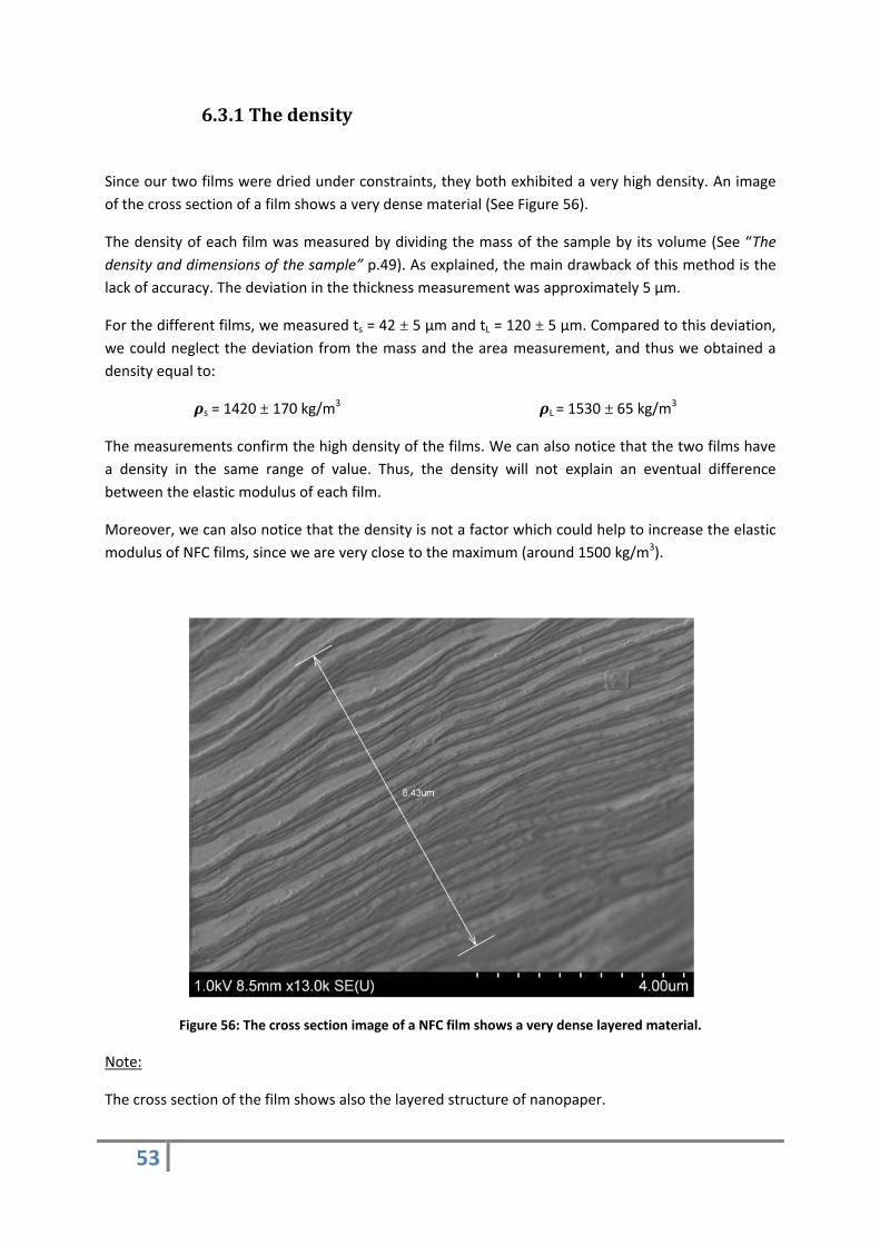
53

6.3.1 The density

Since our two films were dried under constraints, they both exhibited a very high density. An image

of the cross section of a film shows a very dense material (See Figure 56).

The density of each film was measured by dividing the mass of the sample by its volume (See “The

density and dimensions of the sample” p.49). As explained, the main drawback of this method is the

lack of accuracy. The deviation in the thickness measurement was approximately 5 μm.

For the different films, we measured ts = 42 ± 5 μm and tL = 120 ± 5 μm. Compared to this deviation,

we could neglect the deviation from the mass and the area measurement, and thus we obtained a

density equal to:

s = 1420 ± 170 kg/m3 L = 1530 ± 65 kg/m3

The measurements confirm the high density of the films. We can also notice that the two films have

a density in the same range of value. Thus, the density will not explain an eventual difference

between the elastic modulus of each film.

Moreover, we can also notice that the density is not a factor which could help to increase the elastic

modulus of NFC films, since we are very close to the maximum (around 1500 kg/m3).

Figure 56: The cross section image of a NFC film shows a very dense layered material.

Note:

The cross section of the film shows also the layered structure of nanopaper.

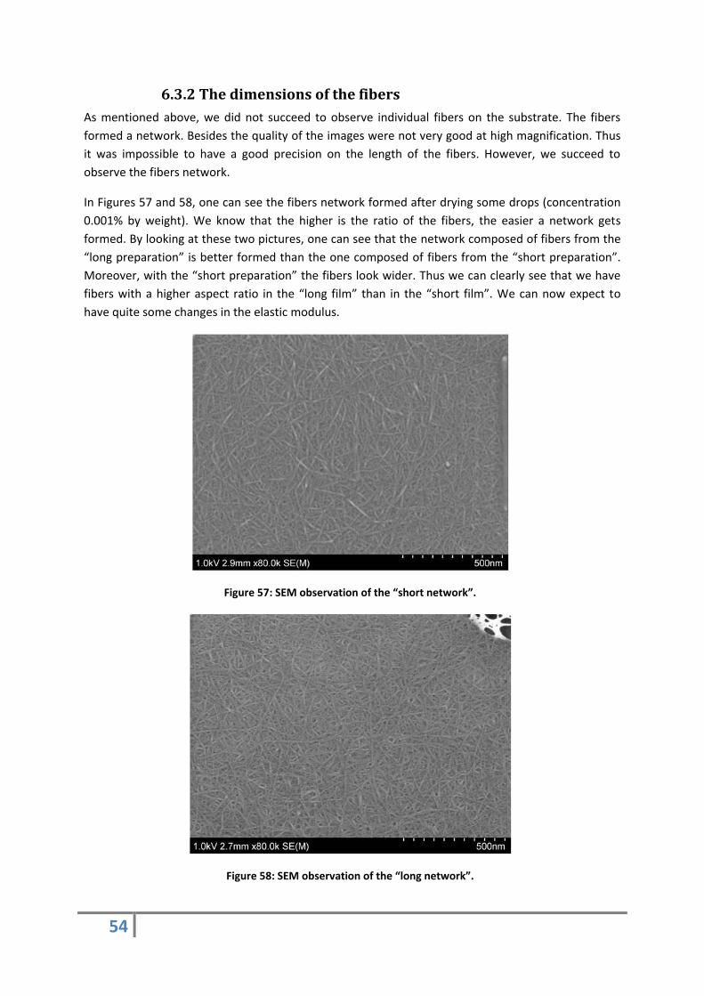
54

6.3.2 The dimensions of the fibers

As mentioned above, we did not succeed to observe individual fibers on the substrate. The fibers

formed a network. Besides the quality of the images were not very good at high magnification. Thus

it was impossible to have a good precision on the length of the fibers. However, we succeed to

observe the fibers network.

In Figures 57 and 58, one can see the fibers network formed after drying some drops (concentration

0.001% by weight). We know that the higher is the ratio of the fibers, the easier a network gets

formed. By looking at these two pictures, one can see that the network composed of fibers from the

“long preparation” is better formed than the one composed of fibers from the “short preparation”.

Moreover, with the “short preparation” the fibers look wider. Thus we can clearly see that we have

fibers with a higher aspect ratio in the “long film” than in the “short film”. We can now expect to

have quite some changes in the elastic modulus.

Figure 57: SEM observation of the “short network”.

Figure 58: SEM observation of the “long network”.

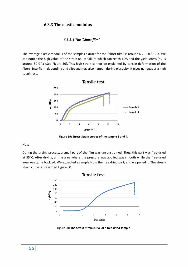
55

6.3.3 The elastic modulus

6.3.3.1 The “short film”

The average elastic modulus of the samples extract for the “short film” is around 6.7 ± 0.5 GPa. We

can notice the high value of the strain (εf) at failure which can reach 10% and the yield stress (σy) is

around 80 GPa (See Figure 59). This high strain cannot be explained by tensile deformation of the

fibers. Interfibril debonding and slippage may also happen during plasticity. It gives nanopaper a high

toughness.

Figure 59: Stress-Strain curves of the sample 3 and 4.

Note:

During the drying process, a small part of the film was unconstrained. Thus, this part was free-dried

at 55°C. After drying, all the area where the pressure was applied was smooth while the free-dried

area was quite buckled. We extracted a sample from the free dried part, and we pulled it. The stress-

strain curve is presented Figure 60.

Figure 60: The Stress-Strain curve of a free dried sample

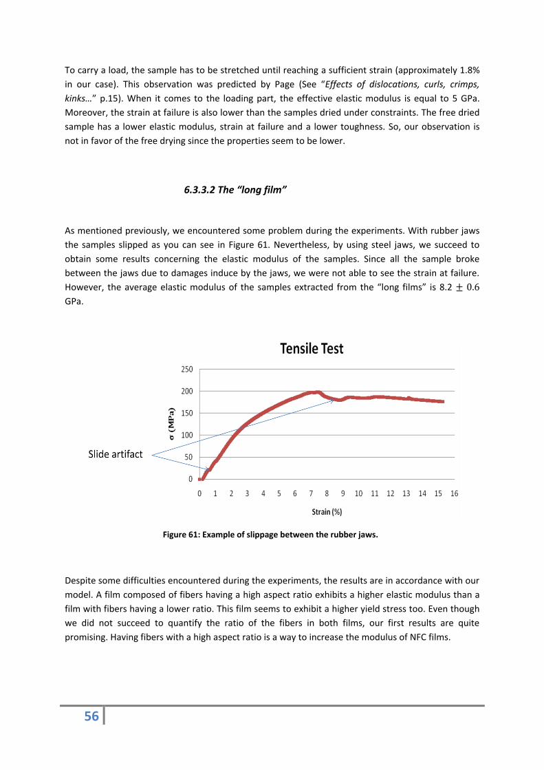
56

To carry a load, the sample has to be stretched until reaching a sufficient strain (approximately 1.8%

in our case). This observation was predicted by Page (See “Effects of dislocations, curls, crimps,

kinks…” p.15). When it comes to the loading part, the effective elastic modulus is equal to 5 GPa.

Moreover, the strain at failure is also lower than the samples dried under constraints. The free dried

sample has a lower elastic modulus, strain at failure and a lower toughness. So, our observation is

not in favor of the free drying since the properties seem to be lower.

6.3.3.2 The “long film”

As mentioned previously, we encountered some problem during the experiments. With rubber jaws

the samples slipped as you can see in Figure 61. Nevertheless, by using steel jaws, we succeed to

obtain some results concerning the elastic modulus of the samples. Since all the sample broke

between the jaws due to damages induce by the jaws, we were not able to see the strain at failure.

However, the average elastic modulus of the samples extracted from the “long films” is 8.2 ± 0.6

GPa.

Figure 61: Example of slippage between the rubber jaws.

Despite some difficulties encountered during the experiments, the results are in accordance with our

model. A film composed of fibers having a high aspect ratio exhibits a higher elastic modulus than a

film with fibers having a lower ratio. This film seems to exhibit a higher yield stress too. Even though

we did not succeed to quantify the ratio of the fibers in both films, our first results are quite

promising. Having fibers with a high aspect ratio is a way to increase the modulus of NFC films.

57

6.3.3.3 NFC Film versus Ordinary Paper.

Some mechanical tests were also done on ordinary paper (printing paper). Our goal was to compare

the mechanical properties of our NFC films versus a standard sheet of paper.

In the plan, while our NFC films have isotropic properties due to the random organization of the

fibers, ordinary paper exhibits different mechanical properties in the plane. Due to the way of

building a paperboard, most of the fibers in commercial paperboard are orientated in the machine

direction (further named MD), which thereby is the stiffest direction. The cross direction (CD) refers

to the cross machine or transverse direction. This is the weakest direction in the plane. This is

illustrated Figure 62.

Figure 62: Paper directions (MD=machine direction, CD= cross machine direction, ZD= normal direction).

Thus, several mechanical tests were done along the CD and MD directions. The different average

results are presented in the Table 5.

Table 5: Mechanical properties of ordinary paper.

Directions MD CD

E (GPa) 2.5 ± 0.2 1.15 ± 0.05

εf (%) 5 ± 0.7 7.5 ± 0.5

σy (Mpa) 25 ± 5 10 ± 2

Regarding the results, one can see a large difference between the mechanical properties of our NFC

films and those of printing paper. The NFC films are stiffer and show a higher total strain. The elastic

modulus is multiplied by 3-4 and the yield stress is increased by a factor greater than 3. It confirms

the great reinforcement potential of cellulose nanofibrils.

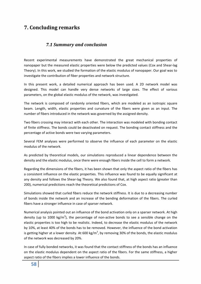
58

7. Concluding remarks

7.1 Summary and conclusion

Recent experimental measurements have demonstrated the great mechanical properties of

nanopaper but the measured elastic properties were below the predicted values (Cox and Shear-lag

Theory). In this work, we studied the formation of the elastic modulus of nanopaper. Our goal was to

investigate the contribution of fiber properties and network structure.

In this present work, a detailed numerical approach has been used. A 2D network model was

designed. This model can handle very dense networks of large sizes. The effect of various

parameters, on the global elastic modulus of the network, was investigated.

The network is composed of randomly oriented fibers, which are modeled as an isotropic square

beam. Length, width, elastic properties and curvature of the fibers were given as an input. The

number of fibers introduced in the network was governed by the assigned density.

Two fibers crossing may interact with each other. The interaction was modeled with bonding contact

of finite stiffness. The bonds could be deactivated on request. The bonding contact stiffness and the

percentage of active bonds were two varying parameters.

Several FEM analyses were performed to observe the influence of each parameter on the elastic

modulus of the network.

As predicted by theoretical models, our simulations reproduced a linear dependence between the

density and the elastic modulus, once there were enough fibers inside the cell to form a network.

Regarding the dimensions of the fibers, it has been shown that only the aspect ratio of the fibers has

a consistent influence on the elastic properties. This influence was found to be equally significant at

any density and follows the Shear-lag Theory. We also found that, at high aspect ratio (greater than

200), numerical predictions reach the theoretical predictions of Cox.

Simulations showed that curled fibers reduce the network stiffness. It is due to a decreasing number

of bonds inside the network and an increase of the bending deformation of the fibers. The curled

fibers have a stronger influence in case of sparser network.

Numerical analysis pointed out an influence of the bond activation only on a sparser network. At high

density (up to 1000 kg/m3), the percentage of non-active bonds to see a sensible change on the

elastic properties is too high to be realistic. Indeed, to decrease the elastic modulus of the network

by 10%, at least 40% of the bonds has to be removed. However, the influence of the bond activation

is getting higher at a lower density. At 600 kg/m3, by removing 30% of the bonds, the elastic modulus

of the network was decreased by 20%.

In case of fully bonded networks, it was found that the contact stiffness of the bonds has an influence

on the elastic modulus dependent on the aspect ratio of the fibers. For the same stiffness, a higher

aspect ratio of the fibers implies a lower influence of the bonds.

59

Simulations showed that the influence of the curled fibers and the bond activation is negligible

compare to the influence of the aspect ratio of the fibers in the range of densities and curl index

values observed in real NFC films.

However, the aspect ratio of the fibers is an important parameter to focus on to increase the elastic

modulus of NFC film. The influence of the aspect ratio was confirmed by experimental

measurements. However, it was impossible to quantify with a great accuracy this parameter inside a

real NFC film. For now, it is speculated to be around 100.

7.2 Future work

Our model showed a good agreement between both theoretical models and experimental

measurements. It motivates an improvement of the network into a more realistic one. Implementing

a 3D structure of the network and a 3D geometry of the bonds could help to understand the

influence of the out-of-plane properties on the elastic modulus of NFC films. A better knowledge of

the properties of the fibers could also improve the model. Investigating the effect of the moisture

and the shrinkage, induce during the drying process, on the properties of nanofibrils could help to

predict the mechanical behavior of NFC films better.

At the same time, further experimental measurements could be done to quantify the aspect ratio of

the fibers.

60

Bibliography

[1] Committee on Synthetic Hierarchical Structures, Commission on Engineering and Technical Systems ,National Research Council. Hierarchical Structures in Biology as a Guide for New Materials Technology. United states: National Academies Press, 1994, 144 p. ISBN-10: 0309046386

[2] Zimmermann T, Bordeanu N, Strub E. Properties of nanofibrillated cellulose from different raw materials and its reinforcement potential. Carbohydrate Polymers, 2010, n. 79, pp. 1086-1093

[3] Anderson R.L., Owens J.W., Timms C.W. The toxicity of purified cellulose in studies with laboratory animals. Cancer Letters, 1992, vol 63, n. 2, pp. 83-92

[4] El Hadjy Babacar LY. Nouveaux matériaux composites thermoformables à base de fibres de cellulose. Grenoble : Institut national polytechnique de Grenoble, 2008, 218 p.

[5] Andresen M., Stenstad P., Møretrø T., Langstrud S., Syverud K., Johansson L-S., Stenius P. Nonleaching antimicrobial films prepared from surface-modified microfibrillated cellulose. Biomacromolecules, 2007, vol 8, pp. 2149-2155

[6] Henriksson M., Berglund L., Isaksson P. et al. Cellulose Nanopaper of High Toughness. Biomacromolecules, 2008, vol 9, n. 6, pp. 1579-1585.

[7] Syverud K, Stenius P. Strength and barrier properties of NFC films. Cellulose, 2009, n. 16, pp.75-85

[8] Berglund L., Eichhorn S.J., Dufresne A. et al. Review: current international research into cellulose nanofibres and nanocomposites. Journal of Materials Science, 2010, n. 45, 33p.

[9] Nishiyama Y., Chanzy H., Langan P. Crystal Structure and Hydrogen Bonding System in Cellulose Iβ from Synchrotron X-ray and Neutron Fiber Diffraction. American Chemical Society, 2002, vol 124, n. 31, 9 p.

[10] Nishiyama Y., Sugiyama J., Chanzy H., Langan P. Crystal Structure and Hydrogen Bonding System in Cellulose Iα from Synchrotron X-ray and Neutron Fiber Diffraction. American Chemical Society, 2003, vol 125, n. 47, 7 p.

[11] Kong K., Eichhorn S.J. The influence of hydrogen bonding on the deformation micromechanics of cellulose fibers. Journal of Macromolecular Sciences, 2005, n. 44, pp. 1123-1136

[12] Sachurada I, Nukushina Y, Ito T. Experimental Determination of the Elastic Modulus of Crystalline Regions in Oriented Polymere. Journal of Polymer Science, 1962, vol 52, pp. 651-660

[13] Tanaka F, Iwata T. Estimation of the elastic modulus of cellulose crystal by molecular mechanics simulation. Cellulose, 2006, vol 13, pp. 509-517

[14] Page D.H., El-Hosseiny F. The mechanical properties of single wood pulp fibres: theories of strength. Fibre Science and Technology, 1975, n. 8, 10 p.

[15] Persson K. Micromechanical modeling of wood and fibre properties. Lund : Lund university, 2000, 213 p.

[16] Alava M., Niskanen K. The physics of paper. Report on Progress in physics, 2006, vol.69, 54 p.

61

[17] Page D.H., El-Hosseiny F., Lancaster A.P.S. Elastic modulus of single wood pulp fibers. Tappi, 1977, vol.60, pp. 114-117

[18] Hsieh Y.C., Yano H., Eichhorn S.J. An estimation of the Young’s modulus of bacterial cellulose filaments. Cellulose, 2008, vol.15, pp. 507-513

[19] Iwamoto S., Kai W., Isogai A., Iwata T. Elastic Modulus of Single Cellulose Microfibrils from Tunicate Measured by Atomic Force Microscopy.Biomacromolecules, 2009, vol.10, pp.2571-2576

[20] Page D.H., Seth R.S. The elastic modulus of paper, II. The importance of fiber modulus, bonding and fiber length. Tappi, 1980, vol.63, n.6, pp. 113-116

[21] Page D.H., Seth R.S. The elastic modulus of paper, III. The effects of dislocations, microcompressions, curl, crimps, and kinks. Tappi, 1980, vol.63, n.10, pp. 99-102

[22] Aström J., Saarinen S., Niskanen K., Kurkijärvi J. Microscopic mechanics of fiber networks. Journal of Applied Physics, 1994, vol.75, n.5, pp 2383-2392

[23] Siro I., Plackett D. Microfibrillated cellulose and new composite materials: a review. Cellulose, 2010, vol.17, pp. 459-494

[24] Nakagaito A.N., Nogi M., Yano H. Displays fromTransparent Films of Natural Nanofibers. MRS Bulletin, 2010, vol. 35, pp. 214-218.

[25] Cox H.L. The elasticity and strength of paper and other fibrous materials. British Journal of Applied Physics, 1952, vol.3, 9 p.

[26] Heyden S. Network modeling for the evaluation of mechanical properties of cellulose fiber fluff. Lund: Lund university, 2000, 209 p.

[27] Aström J., Saarinen S., Niskanen K., Kurkijärvi J. Microscopic mechanics of fiber networks. Journal of Applied Physic, 1994, vol.75, n.5, pp. 2383-2392

[28] Aström J.A, Mäkinen J.P., Alava M.J., Timonen J. Elasticity of Poissonian fiber networks. The American physical society, 2000, vol.61, n.5, pp. 5550-5556

[29] Salminen L.J., Alava M.J., Heyden S., Gustafsson P.J., Niskanen K.J. Simulation of network shrinkage. Nordic Pulp and Paper Research Journal, vol.17, n.2, 6 p.

[30] Mukherjee S., Prathap G. Analysis of delayed convergence in the three noded Timoshenko beam

element using the function space approach.Research report. Bangalore, India: CSIR Centre for

Mathematical Modelling and Computer Simulation, 2001, 32 p.

[31] Hägglund R., Isaksson P. Structural effects on deformation and fracture of random fiber networks

and consequences on continuum models. International Journal of Solids and Structures., 2009, n. 46,

pp. 2320-2329

[32] Lahiji R.R., Xu X., Reifenberger R., Raman A., Rudie A., Moon R.J. Atomic Force Microscopy

Characterization of Cellulose Nanocrystals. Langmuir, 2010, vol.26, n.6, pp. 4480-4488

[33] Wikipedia. Scanning electron microscope [on line]. Available at

<http://en.wikipedia.org/wiki/Scanning_electron_microscope> (24/01/2011)

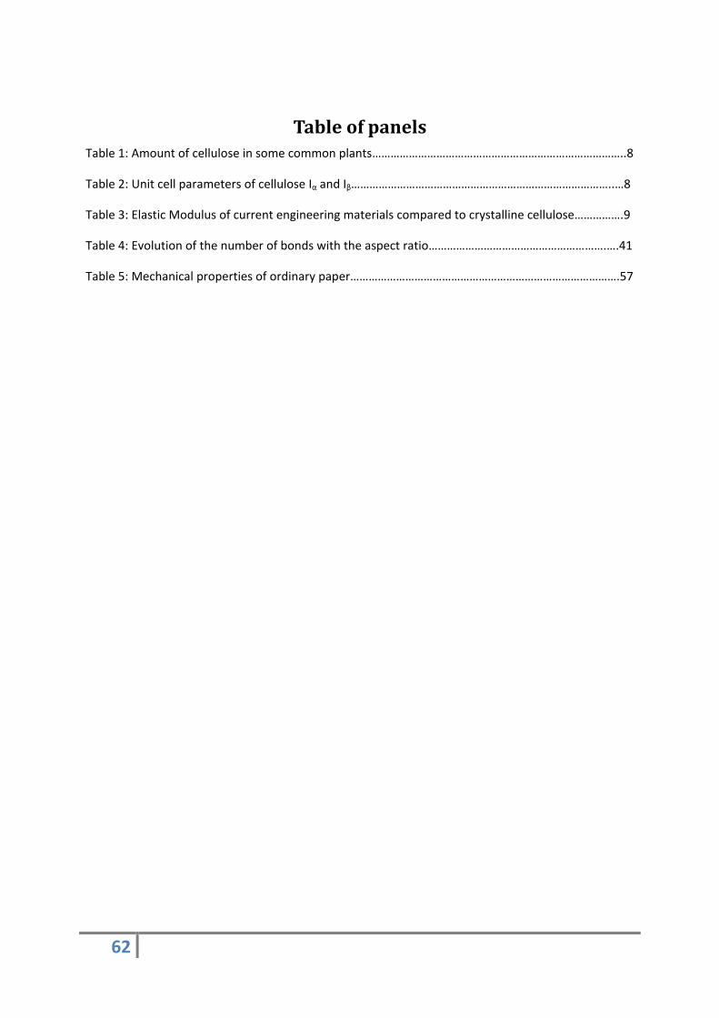
62

Table of panels Table 1: Amount of cellulose in some common plants………………………………………………………………………..8

Table 2: Unit cell parameters of cellulose Iα and Iβ…………………………………………………………………………..…8

Table 3: Elastic Modulus of current engineering materials compared to crystalline cellulose…………….9

Table 4: Evolution of the number of bonds with the aspect ratio………………………………………………….….41

Table 5: Mechanical properties of ordinary paper…………………………………………………………………………….57

63

Table of figures

Figure 1: Wood hierarchy ........................................................................................................................ 6

Figure 2: The paper making process ........................................................................................................ 7

Figure 3: The cellulose structure. ............................................................................................................ 8

Figure 4: The chain structure of native cellulose indicating hydrogen bonding (dotted lines). ............. 9

Figure 5: A single wood fiber with the arrangement of the cellulose in the different layers. .............. 10

Figure 6: Schematic arrangement of the cellulosic fiber inside a layer. ............................................... 10

Figure 7: Action of sodium hydroxide and sodium sulfite to break down the lignin (”kraft” process). 11

Figure 8: Pulp bleaching; the presence of lignin is responsible for the dark color. .............................. 11

Figure 9: A paper machine. ................................................................................................................... 12

Figure 10: The principal axis of the S2 layer (1, 2, 3) and the fiber axes (x, y, z) ................................... 13

Figure 11: Tunicate cellulose is produced by a sea creature; a sea cucumber ..................................... 13

Figure 12: Illustration of the average distribution of axial stress along the fiber [22] ......................... 14

Figure 13: Various states of the fiber and corresponding stress-strain curves a, b, c, d [21] ............... 15

Figure 14: Cellulose nanofiber sheet open the door to new applications ............................................ 16

Figure 15: A Cox network ...................................................................................................................... 18

Figure 16: The Shear-lag theory (a) the stress mechanism (b) the stress distribution along a fiber .... 19

Figure 17: Comparison of the experimental results. ............................................................................. 21

Figure 18: The Cox theory best fit the results obtained by Severud ..................................................... 22

Figure 19: The Poissonian model is closer to the results obtained by Henriksson. .............................. 22

Figure 20: Example of a modeling network fiber with displacement field mapped on the fibers. ....... 23

Figure 21: Type of beam used in the model .......................................................................................... 24

Figure 22: Example of a curled fiber with the definition of the curl index. .......................................... 25

Figure 23: The curl index function C=sin(x)/x from x equals 0 to π. ..................................................... 26

Figure 24: Two fibers crossing are bonded together ............................................................................ 27

Figure 25: A random deposition of the fibers inside the cell. ............................................................... 27

Figure 26: Illustration of fiber modifications to have a periodic cell. ................................................... 28

64

Figure 27: The dashed lines are removed. ............................................................................................ 29

Figure 28: Boundary conditions applied to the network. ..................................................................... 30

Figure 29: Example of a meshing convergence ..................................................................................... 30

Figure 30: Example of a size convergence for a square network .......................................................... 31

Figure 31: Picture of a Bacteria cellulose sheet; a very dense network! .............................................. 32

Figure 32: A homogeneous displacement field. .................................................................................... 33

Figure 33: A homogeneous stress field. ................................................................................................ 34

Figure 34: The influence of the density on the elastic modulus of a fiber network ............................. 34

Figure 35: The influence of the density on the elastic modulus of a fiber network ............................. 35

Figure 36: A network model closes to the Shear-lag predictions ......................................................... 36

Figure 37: Evolution of the elastic modulus, with the ratio, for a 1000 kg/m3 sheet of paper ............. 36

Figure 38: Bonds are modeled as two square areas connected by springs. ......................................... 37

Figure 39: The normalized elastic modulus value functions of the number of bonds at different

density. .................................................................................................................................................. 38

Figure 40: The elastic modulus value functions of the number of bonds at different density. ............ 38

Figure 41: The network elastic modulus function of the bonding stiffness. ......................................... 40

Figure 42: The energy repartition between four deformation processes at different at different

bonding stiffness. .................................................................................................................................. 41

Figure 43: A way to simplify the action of bonds .................................................................................. 42

Figure 44: Different examples of a network with curled fiber (C is respectively equal to 1, 0.9, 0.64) 43

Figure 45: The elastic modulus value functions of the curl index at different density. ........................ 43

Figure 46: The ratio Fc functions of the curl index at different density. ............................................... 44

Figure 47: The energy repartition between three deformation processes for different curl index at a

density of 700 kg/m3. ............................................................................................................................ 45

Figure 48: The energy repartition between three deformation processes for different curl index at a

density of 1300 kg/m3. .......................................................................................................................... 45

Figure 49: AFM micrograph of a “wood cellulose” nanopaper. ............................................................ 46

Figure 50: Obtaining NFC with wood pulp. ........................................................................................... 47

Figure 51: A NFC gel. ............................................................................................................................. 48

65

Figure 52: A gauge. ................................................................................................................................ 49

Figure 53: A tensile test system ............................................................................................................ 50

Figure 54: Schema of a SEM [33]. .......................................................................................................... 51

Figure 55: Cellulose nanocrystals on a mica-PLL substrate. .................................................................. 52

Figure 56: The cross section image of a NFC film shows a very dense material ................................... 53

Figure 57: SEM observation of the “short network”. ............................................................................ 54

Figure 58: SEM observation of the “long network”. ............................................................................. 54

Figure 59: Stress-Strain curves of the sample 3 and 4. ......................................................................... 55

Figure 60: The Stress-Strain curve of a free dried sample .................................................................... 55

Figure 61: Example of slippage between the rubber jaws. ................................................................... 56

Figure 62: Paper directions (MD=machine direction, CD= cross machine direction, ZD= normal

direction). .............................................................................................................................................. 57

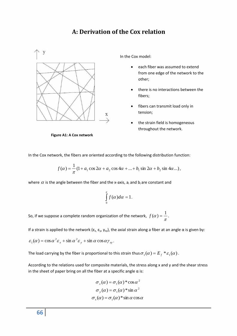
66

A: Derivation of the Cox relation

In the Cox model:

each fiber was assumed to extend

from one edge of the network to the

other;

there is no interactions between the

fibers;

fibers can transmit load only in

tension;

the strain field is homogeneous

throughout the network.

Figure A1: A Cox network

In the Cox network, the fibers are oriented according to the following distribution function:

...)4sin2sin...4cos2cos1(1

)( 2121

bbaaf ,

where is the angle between the fiber and the x-axis, ai and bi are constant and

0

1)( df .

So, if we suppose a complete random organization of the network, .1

)(

f

If a strain is applied to the network (εx, εy, γxy), the axial strain along a fiber at an angle α is given by:

xyyx cossinsincos)( 22

1 .

The load carrying by the fiber is proportional to this strain thus )(*)( 11 fE .

According to the relations used for composite materials, the stress along x and y and the shear stress

in the sheet of paper bring on all the fiber at a specific angle α is:

2

1 cos*)()( x

2

1 sin*)()( y

cossin*)()( 1s

67

So, to have the total stress, we need to multiply the last equations by )(f and integrate over π.

After calculus, we obtain:

yxx EfEf 8

1

8

3

yxy EfEf 8

3

8

1

ss Ef8

1

So finally we obtain C11= C22 = Ef8

3, C12= C66 = Ef

8

1and C16 = C26 =0.

Thus we obtain S11=S22=Ef

3, S12 =

Ef

1, S66 =

Ef

8and S16 =S26=0.

Even if the assumptions of the Cox-model are quite simple, it first found the upper limit for a sheet of

paper having random oriented fibers.

That is to say EfEs3

1 , where Es is the elastic modulus of the sheet and EF the elastic modulus of

the fiber.

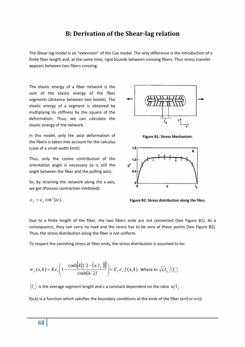
68

B: Derivation of the Shear-lag relation

The Shear-lag model is an “extension” of the Cox model. The only difference is the introduction of a

finite fiber length and, at the same time, rigid bounds between crossing fibers. Thus stress transfer

appears between two fibers crossing.

The elastic energy of a fiber network is the

sum of the elastic energy of the fiber

segments (distance between two bonds). The

elastic energy of a segment is obtained by

multiplying its stiffness by the square of the

deformation. Thus, we can calculate the

elastic energy of the network.

In this model, only the axial deformation of

the fibers is taken into account for the calculus

(case of a small width limit).

Thus, only the cosine contribution of the

orientation angle is necessary (α is still the

angle between the fiber and the pulling axis).

So, by straining the network along the x-axis,

we get (Poisson contraction inhibited):

)(cos 2 xf

Figure B1: Stress Mechanism.

Figure B2: Stress distribution along the fib rs.

Due to a finite length of the fiber, the two fibers ends are not connected (See Figure B1). As a

consequence, they can carry no load and the stress has to be zero at these points (See Figure B2).

Thus, the stress distribution along the fiber is not uniform.

To respect the vanishing stress at fiber ends, the stress distribution is assumed to be:

),(2cosh

21cosh1),( kxfE

k

lxkEkx xf

f

xf

Where k=

sf llc

sl is the average segment length and c a constant dependent on the ratio flw .

f(x,k) is a function which satisfies the boundary conditions at the ends of the fiber (x=0 or x=lf).

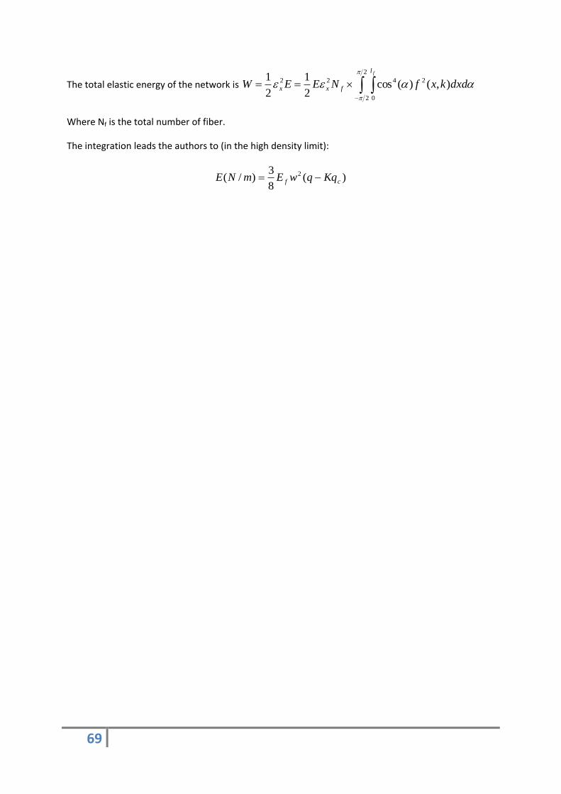
69

The total elastic energy of the network is

2

2 0

2422 ),()(cos2

1

2

1

fl

fxx dxdkxfNEEW

Where Nf is the total number of fiber.

The integration leads the authors to (in the high density limit):

)(8

3)/( 2

cf KqqwEmNE

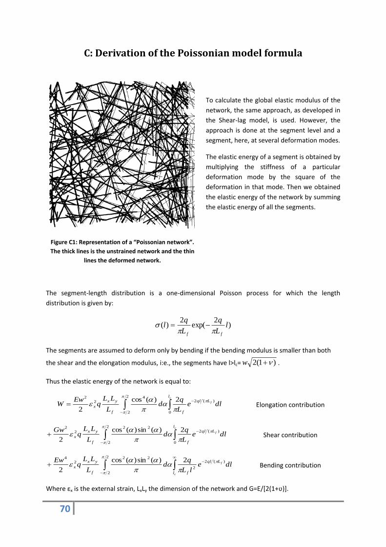
70

C: Derivation of the Poissonian model formula

To calculate the global elastic modulus of the

network, the same approach, as developed in

the Shear-lag model, is used. However, the

approach is done at the segment level and a

segment, here, at several deformation modes.

The elastic energy of a segment is obtained by

multiplying the stiffness of a particular

deformation mode by the square of the

deformation in that mode. Then we obtained

the elastic energy of the network by summing

the elastic energy of all the segments.

Figure C1: Representation of a “Poissonian network”.

The thick lines is the unstrained network and the thin

lines the deformed network.

The segment-length distribution is a one-dimensional Poisson process for which the length

distribution is given by:

)2

exp(2

)( lL

q

L

ql

ff

The segments are assumed to deform only by bending if the bending modulus is smaller than both

the shear and the elongation modulus, i:e., the segments have l>lc= )1(2 w .

Thus the elastic energy of the network is equal to:

2

2 0

)(́24

22 2)(cos

2

c

f

l

Lql

ff

yx

x dleL

qd

L

LLq

EwW Elongation contribution

2

2 0

)(́222

22 2)(sin)(cos

2

c

f

l

Lql

ff

yx

x dleL

qd

L

LLq

Gw Shear contribution

2

2

)(́2

2

222

4 2)(sin)(cos

2

c

f

l

Lql

ff

yx

x dlelL

qd

L

LLq

Ew Bending contribution

Where εx is the external strain, LxLy the dimension of the network and G=E/[2(1+ʋ)].

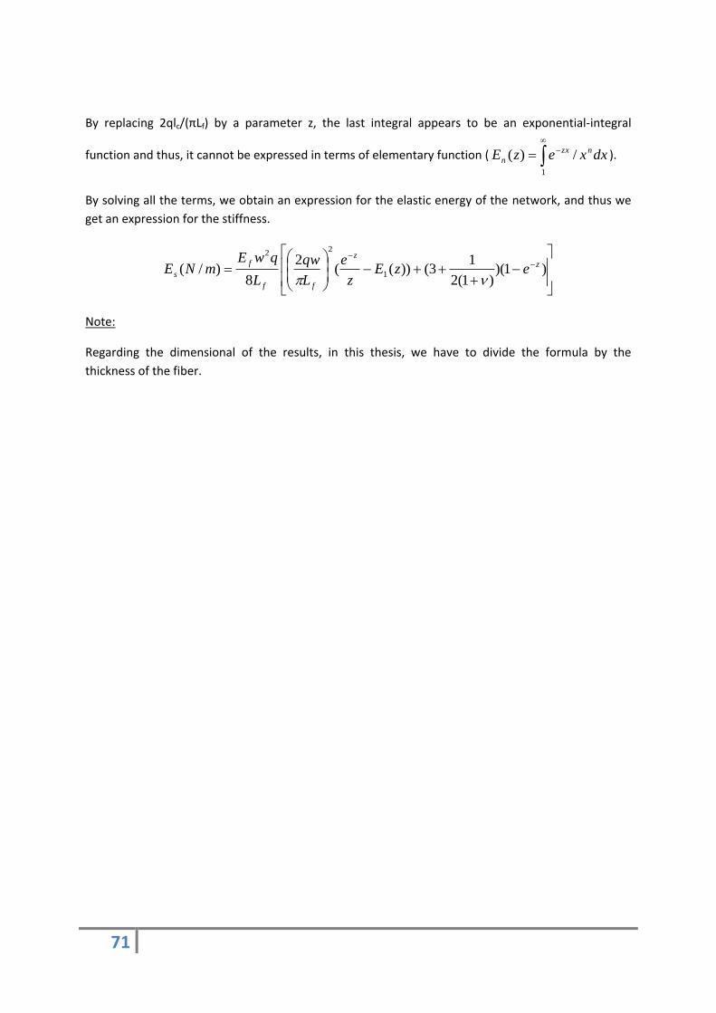
71

By replacing 2qlc/(πLf) by a parameter z, the last integral appears to be an exponential-integral

function and thus, it cannot be expressed in terms of elementary function (

1

/)( dxxezE nzx

n ).

By solving all the terms, we obtain an expression for the elastic energy of the network, and thus we

get an expression for the stiffness.

)1)()1(2

13())((

2

8)/( 1

22

zz

ff

f

s ezEz

e

L

qw

L

qwEmNE

Note:

Regarding the dimensional of the results, in this thesis, we have to divide the formula by the

thickness of the fiber.

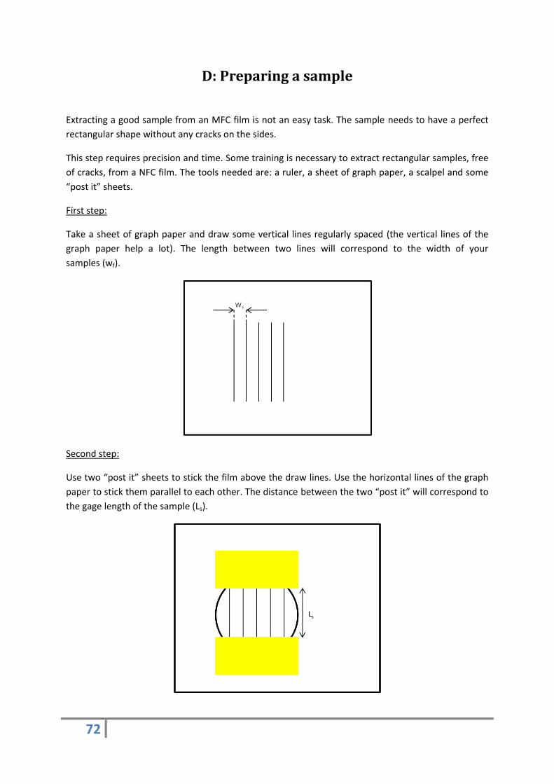
72

D: Preparing a sample

Extracting a good sample from an MFC film is not an easy task. The sample needs to have a perfect

rectangular shape without any cracks on the sides.

This step requires precision and time. Some training is necessary to extract rectangular samples, free

of cracks, from a NFC film. The tools needed are: a ruler, a sheet of graph paper, a scalpel and some

“post it” sheets.

First step:

Take a sheet of graph paper and draw some vertical lines regularly spaced (the vertical lines of the

graph paper help a lot). The length between two lines will correspond to the width of your

samples (wf).

Second step:

Use two “post it” sheets to stick the film above the draw lines. Use the horizontal lines of the graph

paper to stick them parallel to each other. The distance between the two “post it” will correspond to

the gage length of the sample (Ls).

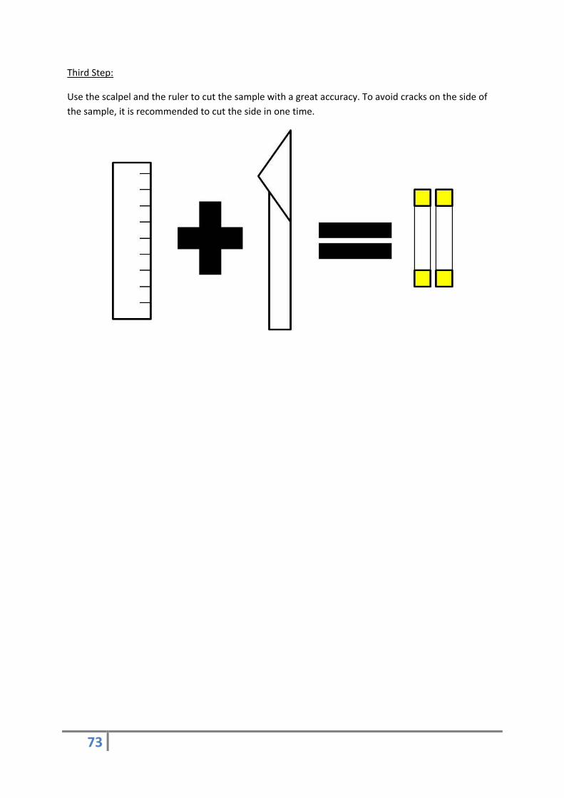
73

Third Step:

Use the scalpel and the ruler to cut the sample with a great accuracy. To avoid cracks on the side of

the sample, it is recommended to cut the side in one time.

74