Mechanical Instabilities of Soft Materials:Creases, Wrinkles, Folds, and Ridges

The Harvard community has made thisarticle openly available. Please share howthis access benefits you. Your story matters

Citation Jin, Lihua. 2014. Mechanical Instabilities of Soft Materials: Creases,Wrinkles, Folds, and Ridges. Doctoral dissertation, HarvardUniversity.

Citable link http://nrs.harvard.edu/urn-3:HUL.InstRepos:13064983

Terms of Use This article was downloaded from Harvard University’s DASHrepository, and is made available under the terms and conditionsapplicable to Other Posted Material, as set forth at http://nrs.harvard.edu/urn-3:HUL.InstRepos:dash.current.terms-of-use#LAA

Mechanical Instabilities of Soft Materials:

Creases, Wrinkles, Folds, and Ridges

A dissertation presented

by

Lihua Jin

to

The School of Engineering and Applied Sciences

in partial fulfillment of the requirements

for the degree of

Doctor of Philosophy

in the subject of

Engineering Sciences

Harvard University

Cambridge, Massachusetts

August, 2014

© 2014 – Lihua Jin

All rights reserved

iii

Thesis Advisor Author

Zhigang Suo Lihua Jin

Mechanical Instabilities of Soft Materials:

Creases, Wrinkles, Folds, and Ridges

Abstract

Subject to a sufficiently large compression, materials may undergo mechanical

instabilities of various types. When the material is homogeneous, creases set in. When the

material is a bilayer consisting of a stiff thin film on a thick compliant substrate, wrinkles set

in. Creases are localized self-contact regions with large strain deviating from the smooth

state, while wrinkles are undulations finite in space with infinitesimal strain deviating from

the smooth state. After the formation of wrinkles, if the compression further increases,

wrinkles double their period and form localized folds. If the substrate is subject to a

sufficiently large pre-tension, wrinkles transit to ridges. This thesis explores different types

of mechanical instabilities: creases, wrinkles, folds, and ridges.

We start with studying creases in different materials. Soft tissues growing under

constraint often form creases. We adopt the model of growth that factors the deformation

gradient into a growth tensor and an elastic deformation tensor, and show that the critical

conditions for the onset of creases take a remarkably simple form. We then perform

simulations to explore creases in strain-stiffening materials. For a solid that stiffens steeply

at large strains, as the compression increases, the surface is initially smooth, then forms

creases, and finally becomes smooth again. For a solid that stiffens steeply at small strains,

iv

creases never form for all levels of compression. In order to better control the formation and

disappearance of creases, we design a soft elastic bilayer with same moduli of the film and

substrate but the substrate pre-compressed, and show that the bilayer can snap between the

flat and creased states reproducibly with tunable hysteresis in a large strain range. We also

show that an interface between two soft materials can form creases under compression.

We then investigate the critical conditions for the onset of wrinkles and creases in

bilayers with arbitrary thicknesses and moduli of the two layers, and show several new types

of bifurcation behavior when the film and substrate have comparable moduli and thicknesses.

We study the effect of substrate pre-stretch on post-wrinkling bifurcations, and show that

pre-tension stabilizes wrinkles while pre-compression destabilizes wrinkles. When the

pre-compression is sufficiently large, ‘chaotic’ morphologies emerge. When the pre-tension is

sufficiently large, we realize ridge localizations and networks under an equi-biaxial

compression, and study the mechanics of ridge formation and propagation.

v

Table of Contents

Title Page …………………………………………………………………………………………….……………………i

Copyright Page ……………………………………………………………………………………………………….ii

Abstract ……………………………………………………………………………………………….…………………iii

Table of Contents ………………………………………………………………….…………..……………………..v

Acknowledgements …………………………………………………………………………….………………….x

Chapter 1 Introduction …………………………………………………………………………………………..1

1.1 Mechanical instabilities ….……………………………………………………………….…….……….1

1.2 Wrinkles and linear perturbation analysis ….……………………………………………………2

1.3 Creases ….……………………………………………………………………………………………………4

1.4 Folds and ridges ……………………………………………………………………………………………6

1.5 Outline of this thesis ………………………………………………………………………………………8

Chapter 2 Creases in soft tissues generated by growth …………………………………..…10

2.1 Introduction …………………...……………………………………………………………….………...10

2.2 Growth model ………………….…………………………………………………………..…………....12

2.3 Critical condition for the initiation of creases due to growth ……………………....14

2.4 Tissue growing in a rigid shell ……………………………………………………………………….15

2.5 Tissue growing outside a rigid core ……………………………….………………………………18

2.6 Number of deep creases …………………………………………………………………………….…21

2.7 Summary …………………………………………………………………………………………………..23

Chapter 3 Smoothening creases on surfaces of strain-stiffening materials ……24

vi

3.1 Introduction ………………….…………………………………………………………………………..24

3.2 Strain-stiffening materials …………………………..……………………………………………...27

3.3 Creases ……………….……………………………………………………………………………………..30

3.4 Wrinkles …………………….…………………………………………………………………………….…35

3.4.1 Two states with small difference in deformation gradient and pressure ……35

3.4.2 Represent general solutions using functions of complex variables ………………36

3.4.3 Critical condition for the onset of wrinkles ………………………………………………39

3.5 Summary ………………….…………………………………………………………………………….…42

Chapter 4 Controlled formation and disappearance of creases ………………………44

4.1 Introduction ……………………….…………………………………………………………………….…44

4.2 Subcritical creases ……………………………………………………………………………………..45

4.3 Methods ………………………………………………………………………………………………………49

4.3.1 Sample preparation ………………………………………………………………………………49

4.3.2 Measurement of viscoelastic properties ……………………………………………………50

4.3.3 Optical and confocal microscope imaging …………………………………………………51

4.3.4 Numerical analysis …………………………………………………………………………………51

4.4 Results ………………………………………………..………………………………………………………53

4.5 Summary …………………………………………..………………………………………………………62

Chapter 5 Creases on the interface between two soft materials …………………….….64

5.1 Introduction …………………..………………………………………………………………………….64

5.2 Analysis and simulations …………………………………………………..………………………..66

5.2.1 Interfacial creases under applied strain ……………………………………………………66

vii

5.2.2 Interfacial creases under both applied strain and pre-strains ……………………74

5.3 Linear perturbation analysis for the onset of interfacial wrinkles ……………………78

5.4 Experimental results …………………………………………………………………………………….81

5.5 Experimental methods …..……………………………………………………………………………83

5.5.1 Experiment with hydrogels confined in a glass slit ……………………………………83

5.5.2 Experiment with thin layers of gels on a glass substrate ……………………………84

5.6 Summary ……………………………………………………………………………………………………86

Chapter 6 The formation of wrinkles or creases in bilayers ……………..……….……..87

6.1 Introduction …………………….………………………………………………………………………….87

6.2 Linear perturbation analysis for wrinkles ………....……………………………………………90

6.2.1 Governing equations and their incremental forms ……………………………………90

6.2.2 Eigenvalue problem ………………………………………………………………………………92

6.2.3 Critical condition for the onset of wrinkles ………………………………………………95

6.3 Subcritical and supercritical creases ….…………………………………………………………99

6.4 Diagram of wrinkles and creases ………………………………..………………………………103

6.5 Summary ………………………………………………………………………….….………………….107

Chapter 7 Role of substrate pre-stretch in post-wrinkling bifurcations …………109

7.1 Introduction ………………….………………………………………………………………………….109

7.2 Methods ……………………………………………………………………………………………………112

7.2.1 Experimental setup ………………………………………………………………………………112

7.2.2 Experimental details ………………………………………………………………………………113

7.2.3 Finite element simulations ……………………………………………………………………115

viii

7.3 Results ………………………………………………………………………………………………………116

7.3.1 Effect of substrate pre-stretch on period doubling ……………………………………116

7.3.2 Chaotic period multiplication under large substrate pre-compression ………121

7.4 Summary ………………………………………………………………………………..………………..131

Chapter 8 Ridge localizations and networks under equi-biaxial loading ……….133

8.1 Introduction …………………..……………...…………………………………………………………133

8.2 Experimental results ....................................................…….....................................135

8.3 Finite element simulations .....................………………………………….....………………142

8.4 Summary ……………………………………………………………………………………………………147

Chapter 9 Mechanics of ridge formation and propagation ……………………….…….149

9.1 Introduction ………………….…..………………………………………………………………………149

9.2 Formation and propagation of ridges ……………........………………………………………151

9.2.1 Static force-displacement method …………………………………………………………153

9.2.2 Pseudo-dynamic loading-unloading method ……………………………………………158

9.2.3 Verification of the two methods ……………………………………………………………163

9.3 Deformation mechanism and geometry of ridges …………………………………………165

9.4 Summary ……………………………………………………………………………………………………172

Chapter 10 Conclusions ......................……......………………………………………………..………174

Bibliography …………………………………………………………………………………………………………178

Appendix ………………………………………………………………………………………………………………205

Appendix A Supporting information for Chapter 3 ……………….……………………………205

A.1 Implementation of the Gent material in ABAQUS ………………………………………205

ix

A.2 Tangent moduli C and matrices A , Q and L of the Gent materials ……206

Appendix B Explicit expression of matrix A in Chapter 6 ……………………………208

Appendix C Supporting information for Chapter 8 ………………………………………………209

C.1 Methods …………………………………………………………………………………………………209

C.2 Supplementary figures ……………………………………………………………………………211

x

Acknowledgements

First and foremost, I would like to bring my heartiest gratitude to my PhD advisor

Professor Zhigang Suo. Zhigang is such an enthusiastic scientist, encouraging mentor and

enlightening teacher. I first met Zhigang at Tongji University in 2008 when I was still a

master student back in China. Zhigang’s talk was extremely illuminative so that I

immediately had the desire to pursue my PhD with him at Harvard. Luckily I was admitted.

In the past five years, I learned from Zhigang in every of our meetings. He has tremendous

knowledge in mechanics, but can express things in the simplest ways. His incredible

inspiration and constant supports keep me making progress. I enjoy taking Zhigang’s courses

and love reading his class notes. He always has the magic to make the classes full of fun and

infect everybody in the classroom with the excitement, but at the same time, gives us deep

understandings and insight to the problems. Zhigang sets the best role model in my research

career.

I am also deeply grateful to Professor Ryan Hayward at University of Massachusetts

Amherst. Most part of my thesis is based on a close collaboration with his group. We have

kept regular Skype meetings in the past three years. His group works on the experimental

side of the projects, and I work on theories. Their beautiful experimental results keep

inspiring new theories and understandings. When our theories predict new phenomena, they

can quickly design experiments and produce the observations. Although as an

experimentalist, Ryan thinks deeper than theoreticians and understands all the details of the

projects. His critical questions in the meetings are always helpful to improve the theories.

xi

I have had the great honor to work with Professor John Hutchinson during my PhD. I

was the teaching fellow in one of his classes, wrote several papers with him, and took a

research class from him, in which we discussed Koiter’s post-buckling analysis. John is one of

the most celebrated scholars in the field of mechanics. Although he has been retired, he can

not stop working on mechanics. John is always supportive and inspiring. His pet phrase is

‘Jesus, how interesting’. I can not imagine how many young researchers he has encouraged in

his career for longer than five decades. I want to express my gratitude and respect to

Professor John Hutchinson.

I also want to thank my committee members, Professor James Rice, Professor Katia

Bertoldi, Professor Lakshminarayanan Mahadevan and Professor Shmuel Rubinstein, for

their suggestions and comments to my research. Jim is another of the most celebrated

scholars in mechanics. It is fabulous for me to read his achievements more than 45 years ago

in textbooks, but at the same time, to knock at his door and discuss with him face to face. Jim

is a devoting teacher. He teaches subjects widely from mathematics to fluid dynamics, from

solid mechanics to geophysics. I was amazed in his classes how things become equally simple

to him as long as they can be described by equations. Katia is an expert on finite element

analysis, and I learned a lot from her class on the finite element method. Most part of my

thesis was done based on the finite element analysis. Therefore, whenever I got frustrated by

the divergence of my simulations, I turned to Katia. Katia is always helpful on improving my

skills of finite element analysis. Maha is the person who created the field of crease instability,

which sets the stage of most of my thesis work. Maha is such a knowledgeable scientist, and

he works on almost everything. His critical questions and comments in talks and seminars

xii

always inspire me to think and to better understand. I thank Shmuel for allowing and guiding

me to do experiments in his lab. He is an encouraging teacher, and I enjoyed all the

discussions with him.

I am grateful to Professor Noel Holbrook and Doctor Fulton Rockwell for leading me

to the new field of plants. I started to discuss with them in my first year in the United States.

My English was not good enough, not to mention English terminology of plants. They were so

kind and patient to go through the basic concepts and phenomena in plants with me, and

introduced me to interesting mechanics problems in plants. I fell in love with plants then,

and will keep an eye on those problems in the future.

I am thankful to my other collaborators. Lots of ideas were brought together and

achievements were realized through the interactions with them. They are Dr. Dayong Chen

(who did the experiments in Chapter 4 and 5) and Anesia Auguste (who did the experiments

in Chapter 7) at Umass Amherst; Dr. Atsushi Takei (who did the experiments in Chapter 8) at

University of Tokyo; Dr. Jia Liu, Prof. Bozhi Tian, Prof. Charles Lieber, Dr. Ramses Martinez,

Prof. George Whitesides, Prof. Adam Abate, Lloyd Han, Prof. David Weitz., Prof. Shengqiang

Cai, Jiawei Yang, Dr. Pengfei Wang, Dr. Jiangshui Huang, Prof. David Clarke, Dian Yang,

Rajiv Desai, Prof Neel Joshi, and Prof. David Mooney at Harvard.

I have also had chances to interact with a number of other distinguished professors at

Harvard and took their classes. I want to thank Prof. Joost Vlassak, Prof. Michael Brenner,

Prof. Frans Spaepen, and Prof. Joanna Aizenberg. They are always kind and open, and

welcome questions. I would also like to thank SEAS academic computing office for their help

on computation softwares.

xiii

It is joyful to work with people in Zhigang’s group. I want to thank all those great

friends: Prof. Nanshu Lu, Prof. Xuanhe Zhao, Dr. Yuhang Hu, Prof. Kejie Zhao, Dr. Matt

Pharr, Prof. Jeong-Yun Sun, Prof. Jian Zhu, Prof. Rui Huang, Prof. Tiefeng Li, Dr. Christoph

Keplinger, Prof. Keith Choon Chiang Foo, Dr. Laurance Brassart, Prof. Adrian Koh, Dr.

Tongqing Lu, Prof. Ronghou Xia, Widusha Illeperuma, Qihan Liu, Jianyu Li, Chao Chen,

Ruobing Bai, Philipp Rothemund, Yecheng Wang, Jianguo Li, Weiss Francois, Zhengjin

Wang, Jingda Tang, Liwu Liu, Huiming Wang and Xin Lan.

I also got lots of helps on finite element analysis from people in Katia’s group. I would

like to thank Prof. Jongmin Shim, Dr. Sung Hoon Kang, Sicong Shan, Jia Liu, Pai Wang and

Sahab Babaee.

I also want to extend my gratitude to other folks in SEAS and friends: Dr. Olga

Dudchenko, Dr. Zhiyan Wei, Dr. Xi Yao, Dr. Hongyan Yuan, Dr. Laura Adams, Dr. Liheng Cai,

Dr. Xinfeng Quan, Dr. Evan Hohlfeld, Omer Gottesman, especially my office mates, Miriam

Huntley, Michael Chemama, Dr. Elizabeth Chen, and my roommates, Jingyi Yu, Yingjun Liu.

Finally, I would bring my deepest gratitude to my parents. They have given me

unconditional love, deep care, constant supports and tremendous understandings. Without

those, I can never go so far on my own.

1

Chapter 1

Introduction

1.1 Mechanical instabilities

Mechanical instabilities are ubiquitous in nature and daily life [1-4]. Instabilities can

form due to various loadings, such as compression, constrained swelling or differential

growth. When the loading is small, the surface of the material keeps smooth. However, when

the loading reaches a critical value, the smooth state loses stability, and the total energy of

the material is minimized by forming instability patterns. Figure 1.1 shows instabilities in a

(a) brain, (b) plant and (c) curtain.

Figure 1.1 Instabilities are ubiquitous in nature and daily life. They are observed in a (a) brain [3],

(b) plant [1], and (c) curtain [2].

In the engineering field, mechanical instabilities used to be thought as modes of

failure, for example, buckling of undersea pipes [5], MEMS [6], and composite materials [7].

However, now people exploit the variety applications of mechanical instabilities [8-12].

Especially, the elastic character of soft materials makes it possible to repeatedly cycle

(a)

(c) (b)

2

between the smooth state and the instability patterns. People use instabilities to fabricate

stretchable electronics [13-18] and microfluidics [19-21], measure material properties [14,

22-26], self-assemble particles [27, 28], align cells [29, 30], reversibly tune adhesion [31-33],

wettability [34-37], friction [38], surface chemistry [39] and optical properties [37, 40-43].

Mechanical instabilities play significant roles in biological systems [44-49], for

example in fingerprint formation [50], embryo invagination [51], gut development [52-55],

brain morphogenesis [56-58], tumor growth [59] and mucus folding [60-63]. The

morphology of viruses [64], plants [65-72] is also related to mechanical instabilities

generated by differential growth or differential swelling.

This thesis studies different types of mechanical instabilities in soft materials: creases,

wrinkles, folds and ridges. Soft materials are usually much more stretchable than stiff

materials, which makes it possible to access new modes of instabilities. Creases [73], folds

[74] and ridges [75] are highly nonlinear modes of instabilities, and they were all identified

in the last several years. The following sections provide an introduction to the different types

of instabilities.

1.2 Wrinkles and linear perturbation analysis

When a bilayer structure with a stiff thin film on a compliant thick substrate is

compressed to a critical load, wrinkles set in to release stress (Figure 1.2). Wrinkles form

periodically in a finite space (Figure 1.2a). The wavelength of wrinkles is determined by a

balance between the deformation of the substrate, which favors short wavelengths, and the

3

bending of the film, which favors long wavelengths [76-79]. When the loading is uniaxial,

parallel wrinkles form perpendicular to the compression direction (Figure 1.2b) [80]. When

the loading is biaxial, complex modes of wrinkles, such as herringbone (Figure 1.2c),

checkerboard and hexagonal, are observed [81-86]. People also studied wrinkles formed

under tensile stretching [87-90], shearing [91, 92] and bending [93, 94].

Figure 1.2 Wrinkle instability. (a) A schematic of wrinkles. (b) Top view of parallel wrinkles formed

under a uniaxial compression [80]. (c) Top view of herringbone mode of wrinkles formed under an

equi-biaxial compression [82]. (d) Cross-section view of parallel wrinkles [95].

Wrinkles have infinitesimal strain deviating from the smooth state and the

cross-sections of wrinkles form smooth undulation (Figure 1.2d). Therefore, a linear

perturbation analysis can be used to predict the critical loading condition and wavelength of

wrinkles [75, 85, 96-99]. A linear perturbation analysis formulates an incremental boundary

value problem with the flat state as a reference, and the onset of wrinkles corresponds to the

existence of a non-trivial solution to the incremental boundary value problem, which is an

eigenvalue problem. Biot used this method to study the surface instability of a hyperelastic

half space [97] and interfacial instability of two hyperelastic half spaces [100]. Modeling both

the film and substrate as linear elastic materials, and considering the thin film as a von

Karman plate under the assumption that the film thickness is much smaller than the

compliant substrate

stiff film (a)

(c) (b)

(d)

4

wavelength of wrinkles, people further developed nonlinear theories of wrinkles [76-79,

101-104], which can not only predict the initiation of wrinkles, but also growth of wrinkles

under small strains.

1.3 Creases

Using a linear perturbation analysis on a semi-infinite neo-Hookean material in

compression, Biot predicted five decades ago that the free surface of an elastomeric half

space would become unstable to the formation of sinusoidal waves upon a critical strain of

0.46 under plane strain condition [97]. However, Biot’s prediction was challenged by

experimental results. Gent and Cho bent a rubber block and observed sharp creases on the

surface at a critical strain of 0.35 [105].

Hohlfeld [73] and Hohlfeld and Mahadevan [106] showed that Biot’s solution and

creases are two distinct instabilities. Biot linearized the boundary value problem around a

state of finite homogeneous deformation, and his solution corresponds to a smooth, wavy

surface (i.e., wrinkles) of small strain relative to the homogeneous state. By contrast, a crease

is a localized, self-contact region of large strain relative to the homogeneous state (Figure

1.3). A crease has a sharp tip, and the cross-section of a crease (Figure 1.3d) looks very

different from that of a wrinkle (Figure 1.2d). Hohlfeld [73] and Hohlfeld and Mahadevan

[106] simulated creases numerically, and found creases set in at a critical strain of 0.354,

which agrees well with the experimental observation of Gent and Cho [105]. The critical

strain for the onset of creases has since been obtained by several other approaches of

numerical analysis [107-111].

5

Figure 1.3 Crease instability. (a) Crease of Liangfen, a starch gel, due to bending [107]. (b) Creases of

rising dough due to the constraint of the bowl [108]. (c) Creases of a swelling gel due to the constraint

of the substrate [112]. (d) Cross-section view of creases [113].

No evidence exists that Biot’s smoothly wavy surfaces have ever been observed

experimentally on homogeneous elastic blocks under compression. Creases, however, have

been observed routinely on elastic blocks compressed by various means, including

mechanical forces [99, 105, 113-116], constrained swelling [112, 117-129], temperature change

[39], electric fields [130-135], and light [136]. Creases have been studied in soft tissues [48,

58, 60]. Creases have been related to the Schallamach waves arising during the frictional

sliding of a rubber against a rigid surface [137], and to the osmotic collapse of a water-filled

cavity in a hydrogel [108].

Surface energy adds a barrier to the nucleation of creases, and makes nucleation

defect-sensitive [119, 138]. When the loading is an electric field, either creases or wrinkles

may form depending on the value of the elastocapillary number [132]. For a layer of finite

(a)

(c) (d)

(b)

6

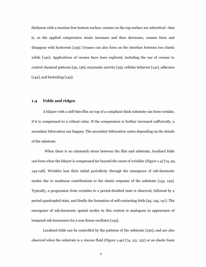
thickness with a traction-free bottom surface, creases on the top surface are subcritical—that

is, as the applied compressive strain increases and then decreases, creases form and

disappear with hysteresis [139]. Creases can also form on the interface between two elastic

solids [140]. Applications of creases have been explored, including the use of creases to

control chemical patterns [39, 136], enzymatic activity [39], cellular behavior [141], adhesion

[142], and biofouling [143].

1.4 Folds and ridges

A bilayer with a stiff thin film on top of a compliant thick substrate can form wrinkle,

if it is compressed to a critical value. If the compression is further increased sufficiently, a

secondary bifurcation can happen. The secondary bifurcation varies depending on the details

of the substrate.

When there is no mismatch stress between the film and substrate, localized folds

can form when the bilayer is compressed far beyond the onset of wrinkles (Figure 1.4) [74, 95,

144-148]. Wrinkles lose their initial periodicity through the emergence of sub-harmonic

modes due to nonlinear contributions to the elastic response of the substrate [145, 149].

Typically, a progression from wrinkles to a period-doubled state is observed, followed by a

period-quadrupled state, and finally the formation of self-contacting folds [95, 145, 147]. The

emergence of sub-harmonic spatial modes in this context is analogous to appearance of

temporal sub-harmonics for a non-linear oscillator [145].

Localized folds can be controlled by the patterns of the substrate [150], and are also

observed when the substrate is a viscous fluid (Figure 1.4a) [74, 151, 152] or an elastic foam

7

[153]. Theoretical studies on fold instability were conducted analytically [74, 145, 149, 154]

and numerically [75, 95]. Geometric patterns in biological interfaces are often far from

idealized sinusoidal wrinkles, but more look like folds. Examples include thread filaments

used by mussel shellfish to adhere to rocks, inner arterial wall and lung surfactants [144].

Figure 1.4 Fold instability. (a) Progression of the folds with increase of strain from top to bottom

when the substrate is a viscous liquid [74, 147]. (b) Progression of the folds with increase of strain

from top to bottom when the substrate is an elastic solid [147].

However, if the substrate is highly pre-stretched, localized ridge instability, instead of

fold, forms as the secondary bifurcation [75, 99, 155-157]. One in every several wrinkles

grows to large amplitude to form ridges, and leave the neighboring wrinkles flattened (Figure

1.5). Although both folds and ridges are localized, their morphologies look very different.

Folds grow inwards and fold up the surface, while ridges grow outwards and lift up the

surface (Figure 1.5). If the substrate is not pre-stretched, folds form as a secondary

bifurcation from wrinkles [145]; if the substrate is pre-tensioned mildly, wrinkles can sustain

larger compression without a secondary bifurcation and form a shape with high aspect ratio

[158]; if the pre-tension is large enough, ridges form at a relatively small compressive strain

[75, 99, 155-157]. All these various behavior can be explained by the highly nonlinear

elasticity of the substrate [155]. A pre-tension of the substrate favors the occurrence of

outward deflections of the surface, while a pre-compression favors inward deflections [155].

(a) (b)

8

Ridge instability was first observed and predicted by a numerical simulation [75], and

then was realized in experiments [99, 155-157]. Large aspect ratio of the ridge instability

facilitates its applications in reversible wettability tuning and stem cells alignment [156].

Figure 1.5 Ridge instability. (a) Simulation result showing the cross-section view of a secondary

bifurcation from wrinkles to ridges [75]. (b) Experimental results showing the top view of ridges [156].

1.5 Outline of this thesis

This thesis studies the different types of mechanical instabilities: creases, wrinkles,

folds, and ridges. In Chapter 2, we model growth in soft tissues and study creases generated

by growth analytically and numerically. In Chapter 3, we perform numerical simulations to

examine initiation and evolution of creases in strain-stiffening materials. In Chapter 4, we

design a soft elastic bilayer to better control the formation and disappearance of creases

based on a joint experimental and theoretical study. In Chapter 5, we perform simulations

and experiments to show that an interface between two soft materials can form creases

under compression. In Chapter 6, we investigate the critical conditions for the formation of

wrinkles and creases in bilayers with arbitrary thicknesses and moduli of the two layers. In

Chapter 7, we explore the effect of pre-stretch in the substrate on the post-wrinkling

bifurcations in bilayers experimentally and theoretically. In Chapter 8, we experimentally

realize the ridge localizations and networks by incremental release of the equi-biaxial

(a) (b)

9

pre-stretch in the substrate with a microfluidic device, and theoretically simulate ridges and

obtain the critical conditions for the formation of ridges. In Chapter 9, we perform numerical

simulations to analyze the mechanics of ridge formation and propagation. Chapter 10

provides conclusions of this thesis.

10

Chapter 2

Creases in soft tissues generated by growth

2.1 Introduction

Soft tissues often grow under constraint. For example, many tubular organs—arteries,

airways, esophagi and intestines—grow under the constraint of a stiffer tissue, the smooth

muscle [62, 159]. Some tumors grow under the constraint of necrotic cores [160]. Even in the

absence of any stiff tissues, soft tissues develop internal constraint when the growth is

inhomogeneous [161]. Constrained growth can cause the soft tissues to undulate and fold.

These mechanical instabilities have physiological and pathological consequences [50, 51, 60,

65, 160, 162, 163]. When the smooth muscle of airways shortens, the mucosa folds and

obstructs the airways; the amount of obstruction increases in asthma due to the thickening

of the airway walls [162, 163]. Buckling can enable the invagination of embryos [51], and the

primordial development of sunflowers [65]. Fingerprint patterns can result from the

buckling of the layer of basal cells of the fetal epidermis [50]. The shape of a tumor can

indicate its type [160].

Figure 2.1 illustrates several ubiquitous patterns of instability. For a soft material

covered with a stiff thin layer, compression beyond a critical level leads to wrinkles [81].

Further compression will turn some of the wrinkles into folds [74, 95]. For a soft material

not covered with a stiff layer, however, compression beyond a critical level leads to creases,

without forming wrinkles first [106-109, 112, 113, 164]. While the wrinkles keep the surface

11

of the material locally smooth, the folds and creases cause the surface to self-contact. The tip

of a fold remains open due to the bending rigidity of the stiff layer, but the tip of a crease is

sharp.

Figure 2.1 Schematic illustrations of three ubiquitous patterns of mechanical instability.

The onset of wrinkles corresponds to superposing a field of strain infinitesimal in

amplitude, but finite in space. By contrast, the onset of creases corresponds to superposing a

field of strain finite in amplitude, but infinitesimal in space. Consequently, the critical

condition for the onset of wrinkles can be determined by a classical linear perturbation

analysis, while the critical condition for the onset of creases cannot. Several recent papers

have studied creases in soft materials caused by external forces [106-109, 113, 164].

This chapter studies creases in tissues undergoing constrained growth. We show that

the critical conditions for the onset of the growth-induced creases take a remarkably simple

form. The critical conditions are illustrated with tubes of tissues growing either inside a rigid

shell or outside a rigid core. Furthermore, deep creases in a tube are simulated by using the

finite-element method, and the number of creases is estimated by minimizing the free

energy.

12

2.2 Growth model

As illustrated in Figure 2.2, we adopt a well-known model of growth [165]. A tissue is

taken to be stress-free before the growth. An unconstrained and homogeneous growth

changes the size of the tissue, but does not induce any stress. The stress-free growth is

characterized by a growth tensor, G, which maps any vector in the tissue in the stress-free

state to a vector in the tissue after the growth by a stretch and a rotation. To model the

constrained and inhomogeneous growth, we think of the tissue as many small elements, and

name each element by its coordinate X when the tissue is in the stress-free state. The growth

of the element is characterized by a growth tensor ( )XG , which may vary from one element

to another. If only the stress-free growth tensor were considered, the neighboring elements

would not fit together after the growth, but would have gaps or overlaps [166]. This

incompatible, stress-free state after the growth is illustrated in Figure. 2.2 To make the

elements compatible with one another, and to satisfy the constraint imposed by surrounding

stiff tissues, each element deforms, which is characterized by a deformation tensor, ( )XA .

The multiplication of the growth tensor and the deformation tensor gives the deformation

gradient [165]:

AGF = . (2.1)

As illustrated in Figure. 2.2, ( )XG maps the tissue from the stress-free state before the

growth to the stress-free state after the growth, ( )XA maps the tissue from the stress-free

state after the growth to the stressed state after the growth, and the deformation gradient

( )XF maps the tissue from the stress-free state before the growth to the stressed state after

the growth. While both ( )XG and ( )XA may be incompatible, their multiplication ( )XF

13

is compatible [166, 167].

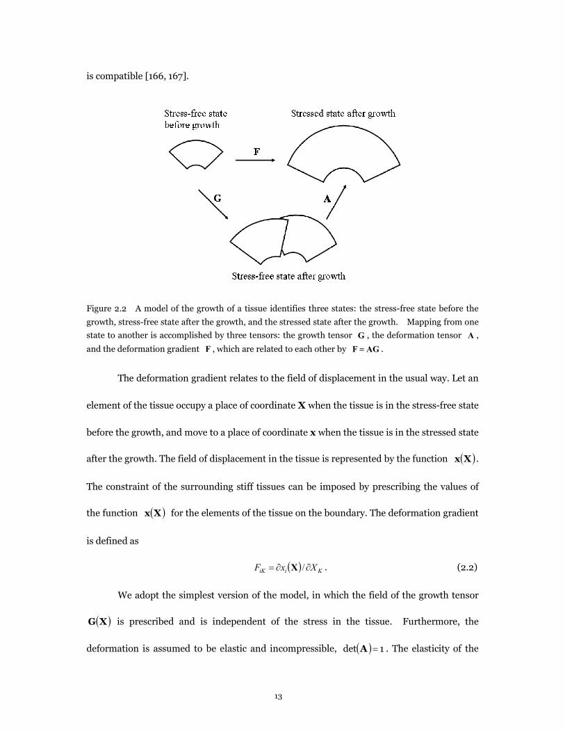
Figure 2.2 A model of the growth of a tissue identifies three states: the stress-free state before the

growth, stress-free state after the growth, and the stressed state after the growth. Mapping from one

state to another is accomplished by three tensors: the growth tensor G , the deformation tensor A ,

and the deformation gradient F , which are related to each other by AGF = .

The deformation gradient relates to the field of displacement in the usual way. Let an

element of the tissue occupy a place of coordinate X when the tissue is in the stress-free state

before the growth, and move to a place of coordinate x when the tissue is in the stressed state

after the growth. The field of displacement in the tissue is represented by the function ( )Xx .

The constraint of the surrounding stiff tissues can be imposed by prescribing the values of

the function ( )Xx for the elements of the tissue on the boundary. The deformation gradient

is defined as

( ) KiiK XxF ¶¶= /X . (2.2)

We adopt the simplest version of the model, in which the field of the growth tensor

( )XG is prescribed and is independent of the stress in the tissue. Furthermore, the

deformation is assumed to be elastic and incompressible, ( ) 1det =A . The elasticity of the

14

tissue is assumed to be neo-Hookean and isotropic, so that the elastic energy of the tissue is

( ) ( ) -=P dVT GAA det32

trm

, (2.3)

where m is the shear modulus. The integral extends over the volume of the tissue in the

stress-free state before the growth, and ( )Gdet is the volume after the growth divided by

that before the growth. If the body is subject to mechanical forces, the potential energy of the

forces need be added to (2.3). The total free energy is minimized subject to the constraint

( ) 1det =A and the boundary conditions of ( )Xx .

2.3 Critical condition for the initiation of creases due to growth

Before creases set in, the surface of the tissue is smooth, and every element on the

surface is in a well-defined state of strain. When the state of strain of an element reaches a

critical condition, a crease sets in at this element—that is, the onset of each crease is

autonomous [106-108]. For a neo-Hookean material subject to external forces, the critical

conditions for the onset of creases have been calculated for general states of strain [107]. We

now apply these conditions to tissues growing under constraint. Within the model of growth

illustrated in Figure 2.2, the stress is developed in going from the stress-free state after the

growth to the stressed state after the growth. Consequently, the critical conditions for the

onset of creases obtained in [107] should be applied to the elastic deformation tensor ( )XA .

For an element X on the surface of the tissue, the three eigenvalues of AA T are

denoted by 2

3

2

2

2

1 ,, aaa —that is, 321 ,, aaa are the principal elastic stretches. The surface of

the tissue is assumed to be traction free, so that the direction normal to the surface is a

principal direction of the stress tensor and, for a material of isotropic elasticity, is also a

15

principal direction of the elastic deformation tensor. The other two principal directions are

tangential to the surface of the tissue. We label the direction normal to the surface as

direction 3, and the other two principal directions as directions 1 and 2. The critical

condition for the onset of a crease normal to direction 1 is

4.2/ 13 =aa , (2.4)

while the critical condition for the onset of a crease normal to direction 2 is

4.2/ 23 =aa . (2.5)

The value 4.2 was obtained for the incompressible neo-Hookean material by finite element

calculation in [107], in which the critical condition for the onset of crease is defined as the

condition when the elastic energy of creased state equals the smooth state. Creases will form

first in the direction with the lower value in 1a and 2a . If 21 aa = , creases may form in any

direction inside the surface.

2.4 Tissue growing in a rigid shell

We next illustrate the critical conditions with examples. Figure 2.3 shows a tube of a

tissue growing in a rigid shell. In the stress-free state before the growth, the tube is of radii A

and B. In the stressed state after the growth, the tube is of radii a and B. The rigid shell

constrains the growth, and the soft tissue is perfectly bonded to the rigid shell, so that after

the growth the outer radius and the length of the tube remain unchanged. Since the length of

the tube is large compared to the radii, we assume that the tissue deforms under the

plane-strain conditions. The growth tensor is assumed to be of the form ],,[diag zr ggg =G ,

where zr ggg ,, are the growth ratios in the radial, circumferential, and longitudinal

16

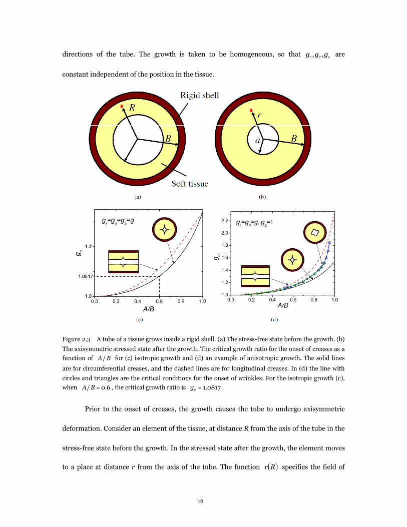
directions of the tube. The growth is taken to be homogeneous, so that zr ggg ,, are

constant independent of the position in the tissue.

Figure 2.3 A tube of a tissue grows inside a rigid shell. (a) The stress-free state before the growth. (b)

The axisymmetric stressed state after the growth. The critical growth ratio for the onset of creases as a

function of BA/ for (c) isotropic growth and (d) an example of anisotropic growth. The solid lines

are for circumferential creases, and the dashed lines are for longitudinal creases. In (d) the line with

circles and triangles are the critical conditions for the onset of wrinkles. For the isotropic growth (c),

when 6.0=/ BA , the critical growth ratio is 0817.1=cg .

Prior to the onset of creases, the growth causes the tube to undergo axisymmetric

deformation. Consider an element of the tissue, at distance R from the axis of the tube in the

stress-free state before the growth. In the stressed state after the growth, the element moves

to a place at distance r from the axis of the tube. The function ( )Rr specifies the field of

17

displacement. Because the elastic deformation is taken to be incompressible, the increase in

the volume of the tube is entirely due to the growth. Consider an annulus between the radii B

and R in the stress-free state before the growth, and between the radii B and r in the stressed

state after the growth. The growth increases the volume of the annulus by factor zr ggg , so

that

( )2222 RBgggrB zr -=- . (2.6)

This expression specifies the field of displacement, the function ( )Rr . To prevent the tissue

from interpenetrating after the growth, we require that 0>a . Inserting this condition into

(6), we obtain that ( )222 ABgggB zr -> . The deformation gradient takes the form

zr lll ,,diag=F , with the principal stretches being ll /zrr ggg= , Rr /=l , and 1=zl .

The elastic deformation tensor takes the form zr aaa ,,diag=A , with the principal

elastic stretches being rrr g/la = , la g/= , zzz g/la = .

Following (2.4) and (2.5), the critical condition for the onset of circumferential

creases is 4.2/ =aar at the surface of the tube AR = , or

4.212

2

2

22

=

--

A

Bggg

A

Bgg zrz . (2.7)

The critical condition for the onset of longitudinal creases is 4.2/ =zr aa at the surface of

the tube AR = , or

4.212

2

2

22

=

--

A

Bggg

A

Bgg zrz . (2.8)

In the limit 0/ ®BA , any growth 1>zr ggg will cause very large compressive

elastic strain at the inner surface of the tube, so that the critical condition for the onset of

creases is 1=zr ggg . In the limit 1/ ®BA , the tube behaves like a flat layer constrained by

18

a rigid substrate, so that the critical condition for the onset of the circumferential creases is

4.22 =zgg , and the critical condition for the onset of the longitudinal creases is 4.22 =zgg .

For isotropic growth, gggg zr === , Figure. 2.3c plots the critical growth ratio cg

for the onset of creases as a function of BA/ . The solid curve represents the critical

condition for the onset of circumferential creases, and the dashed curve represents the

critical condition for the onset of longitudinal creases. For both types of creases, 1=cg in

the limit 0/ →BA , and 3 4.2=cg in the limit 1/ →BA . Between the two limits, the

growth ratio needed to initiate the circumferential creases is less than that needed to initiate

the longitudinal creases.

As an example of anisotropic growth, consider the growth ratios gggr == and

1=zg . Figure 2.3d plots the critical growth ratio cg for the onset of creases as a function of

BA/ . In the limit 1/ →BA , 4.2=cg for the onset of the circumferential creases and

4.2=cg for the onset of the longitudinal creases. In this example, the growth needed to

initiate the circumferential creases is less than that needed to initiate the longitudinal

creases. Also included in Figure 2.3d are the critical conditions for the onset of

circumferential wrinkles obtained by the linear perturbation analysis (circles from [159] and

triangles from [168]). A comparison of these results in Figure 2.3d indicates that the

circumferential creases will set in, rather than the circumferential wrinkles.

2.5 Tissue growing outside a rigid core

19

Figure 2.4 A tube of a tissue grows outside a rigid core. (a) The stress-free state before the growth.

(b) The axisymmetric stressed state after the growth. The critical growth ratio for the onset of creases

as a function of BA/ for (c) isotropic growth and (d) an example of anisotropic growth. The solid

lines are for circumferential creases, and the dashed lines are for longitudinal creases.

Figure 2.4 illustrates a tube of a tissue growing outside a rigid core. The tube is of

radii A and B in the stress-free state before the growth, and is of radii A and b in the

stressed state after the growth. Prior to the onset of creases, the growth causes axisymmetric

deformation in the tube. The field of deformation ( )Rr is determined by

( )2222 ARgggAr zr -=- . (2.9)

The critical condition for the onset of circumferential creases on the outer surface of the tube

20

is

4.212

2

2

22

=

--

B

Aggg

B

Agg zrz . (2.10)

The critical condition for the onset of longitudinal creases on the outer surface of the tube is

4.212

2

2

22

=

--

B

Aggg

B

Agg zrz . (2.11)

In the limit 0/ ®BA , the rigid core becomes a thin needle, and the critical conditions for

the onset of the circumferential and longitudinal creases become 4.2=rgg and

4.23

=rz ggg . In the limit 1/ ®BA , the tube behaves like a flat layer constrained by a

rigid substrate, which has been discussed above.

For the isotropic growth gggg zr === , Figure 2.4c plots the critical level of growth

cg for the onset of creases as a function of BA/ . The critical condition for the onset of

circumferential creases can only be satisfied when 12/7/ >BA . Below this value, the rigid

core does not provide sufficient constraint to cause circumferential creases on the outer

surface of the tube. At all values of BA/ , longitudinal creases will set in before

circumferential creases. By contrast, in the case of anisotropic growth, gggg zr =,1== ,

circumferential creases can form in the entire range of BA/ , and can form before

longitudinal creases, Figure 2.4d. In [122], the swelling of a gel under constraint was studied

in the similar geometry. When the core is much stiffer than the swelling gel, sharp creases

were observed in the gel. The linear perturbation analysis in [122] assumed infinitesimal

strains from the smooth state, and corresponds to an analysis of wrinkling. By contrast, our

analysis based on the result of nonlinear finite element method allows large strains from the

smooth state, and corresponds to creases.

21

2.6 Number of deep creases

Because the state of strain is invariant everywhere on the surface of the tube under

the axisymmetric deformation, every point on the surface reaches the critical condition to

initiate a crease simultaneously. Consequently, the condition for the onset of creases does

not determine the number of creases in a tube. In order to determine the number of creases,

we go beyond the initiation of the creases and analyze deep creases. The analysis is carried

out by using the commercial finite-element software ABAQUS, in which the growth of soft

tissues can be simulated by thermal expansion. Plane strain conditions are assumed.

Symmetry is assumed such that if the number of creases is N , we only need to simulate one

part of the tube within angle N/ . Following [113], we prescribe the nucleus of a crease by

placing a defect, a quarter of a circle with small radius, on the surface of the tube. To

eliminate the effect of the defect, its size is made much smaller than the thickness of the tube.

At the same time, to resolve the field close to the defect, the size of the elements close to the

defect is made much smaller than the size of the defect. The surface of the tube is allowed to

self-contact.

As an example, consider a tube of a tissue growing inside a rigid shell, with

6.0/ =BA . The growth is taken to be isotropic, and the elasticity neo-Hookean. The

finite-element calculation determines the free energy per unit thickness of the tube as a

function of the growth ratio, )(gP . The free energy per thickness of the axisymmetric

deformation without creases can be calculated analytically, according to (2.3):

( ) ( ) ( )( )

ù

é--++

+--=P 2223

2

222332

0 312log12

ABggA

BBAggB

gm. (2.12)

Figure 2.5 shows the ratio 0/PP as a function of the growth ratio g for several cases of

22

prescribed numbers of defects. When g is small, 1/ 0 =PP , and the defects do not cause

the surface to self-contact and become creased. Beyond a critical value 085.1=cg , however,

0/PP < 1, and the defects cause the surface to self-contact and become creased. This

critical value is consistent with the analytical prediction for the onset of creases 0817.1=cg

as shown in Figure 2.3c. Right after the initiation, individual creases do not interact, so that

more creases can release more energy. With the further growth, the creases deepen and

interact with one another. As shown in Figure 2.5, the energy in the tube with seven creases

is lowest when 1033.1<g . After that the tube with six creases has the lowest energy until

1291.1=g , and then the tube with five creases has the lowest energy. Figure 2.6 shows the

creased states of the tube with different prescribed numbers of creases at different growth

ratios. The color indicates the value of the von Mises stress.

Figure 2.5 For a tube of a tissue growing inside a rigid shell, the ratio of the elastic energy of the

creased state to that of the axisymmetric state, 0/PP , is plotted as a function of the growth ratio, g .

The inset enlarges the squared region.

23

Figure 2.6 Deep creases develop from the surface of a tube of a tissue growing inside a rigid shell.

Different numbers of creases are prescribed. The color indicates the level of the von Mises stress.

2.7 Summary

In summary, we obtain the critical conditions for the onset of creases caused by

constrained growth. The critical conditions are illustrated with tubes of soft tissues growing

under the constraint of either rigid outer shells or rigid inner cores. By comparing with the

critical conditions for the onset of wrinkles, we show that creases are preferred type of

instability. Deep creases are simulated by using the finite-element method. The number of

deep creases in a tube may be determined by minimizing the free energy.

24

Chapter 3

Smoothening creases on surfaces of strain-stiffening

materials

3.1 Introduction

Biot analyzed an elastic block compressed under the plane strain conditions (Figure

3.1a, b), and predicted that the flat surface of the block was unstable when the compression

reached a critical strain of 0.46 [97]. This theoretical prediction remained unchallenged until

Gent and Cho noted its disagreement with their experimental finding that the surface formed

creases at a critical strain of 0.35 [105]. Hohlfeld and Mahadevan showed that Biot’s solution

and creases are two distinct instabilities, and that creases set in at a critical strain of 0.35 [73,

106]. Biot linearized the boundary-value problem around a state of finite homogeneous

deformation, and his solution corresponds to a smooth, wavy surface (i.e., wrinkles) of small

strain relative to the homogeneous state (Figure 3.1c). By contrast, a crease is a localized,

self-contact region of large strain relative to the homogeneous state (Figure 3.1d). The critical

strain for the onset of creases has since been obtained by several other approaches of

numerical analysis [107-111]. Furthermore, Hohlfeld mapped the onset of a crease to the

coexistence of two scale-invariant states [169]. A post-bifurcation analysis of Cao and

Hutchinson showed that Biot’s solution is unstable [164].

25

Figure 3.1 (a) In the stress-free state, a block of elastic material is of width W and height H. Under

compression the material may deform in several ways. (b) The block undergoes homogeneous

compression. (c) The surface forms wrinkles. (d) The surface forms a crease of crease depth L. The

applied strain e is defined by the compressive displacement divided by the initial width of the block.

No evidence exists that Biot’s smoothly wavy surfaces have ever been observed

experimentally on homogeneous elastic blocks under compression. Creases, however, have

been observed routinely on elastic blocks [39, 99, 105, 112-118, 120-128, 130-136]. Creases

have been studied in soft tissues [48, 58, 60]. Creases have been related to the Schallamach

waves arising during the frictional sliding of a rubber against a rigid surface [137], and to the

osmotic collapse of a water-filled cavity in a hydrogel [108]. Creases can also form on the

interface between two elastic solids [140]. Applications of creases have been explored,

including the use of creases to remove control chemical patterns [39, 136], enzymatic activity

[39], cellular behavior [141], adhesion [142], and biofouling [143].

Although wrinkles have never been observed experimentally on large homogeneous

elastic blocks under compression, many factors affect the behavior of creases, and may even

26

promote the formation of wrinkles. Surface energy adds a barrier to the nucleation of creases,

and makes nucleation defect-sensitive [119, 138]. When the loading is an electric field,

wrinkles may form when the elastocapillary effect is strong enough [132]. For a layer of finite

thickness with a traction-free bottom surface, creases on the top surface are subcritical—that

is, as the applied compressive strain increases and then decreases, creases form and

disappear with hysteresis [139]. For a stiff film on a soft substrate under compression, the

film forms periodic wrinkles at a small strain [81]. As the strain increases, the wrinkles

double their period, and ultimately lead to deep folds [74]. When the film and the substrate

have comparable moduli, the transitions between creases, wrinkles and folds become

complex [99, 170]. Complex behavior also occurs in a solid of gradient modulus [171, 172].

If the substrate is pre-compressed, creases are subcritical, and form and disappear with

hysteresis [173].

Biot’s original analysis, as well as much of the subsequent theoretical work,

represents the elastic solid by the neo-Hookean model. This model describes elastomers of

long polymer chains well, but is inadequate when materials stiffen steeply. A soft biological

tissue, for example, is usually a composite of a compliant matrix and stiff fibers [174]. When

the tissue is under a small strain, the matrix carries much of the load, but the fibers are not

tight, so that the tissue is soft. As the strain increases, the fibers gradually tighten and rotate

to the loading direction, so that the tissue stiffens steeply. As another example, an elastomer

is a three-dimensional network of long and flexible polymer chains [175]. When the

elastomer is under no stress, the chains undergo thermal motion and coil. When the

elastomer is subject to moderate strains, the chains uncoil and the stress-strain relation of

27

the elastomer is well represented by the neo-Hookean model, which is derived under the

assumption of Gaussian chains. When the chains become nearly straight, however, they no

longer obey the Gaussian statistics, and the stress-strain curve rises steeply and deviates

significantly from the neo-Hookean model. Destrade et al. analyzed the onset of wrinkles on

the surface of a bending block [94]. They showed that when the material stiffens at a

relatively small strain, the critical strain for the onset of wrinkles differs significantly from

that of a neo-Hookean material. These authors, however, did not consider the formation of

creases.

In this chapter, we represent a strain-stiffening material by using the Gent model

[176], and study the initiation and development of creases by using a finite element method.

For a solid that stiffens at large strains, as the compression increases, the surface is initially

smooth, then forms creases, and finally becomes smooth again. For a solid that stiffens at

small strains, creases will never form and the surface remains smooth for all levels of

compression. We also study the condition for the onset of wrinkles by using linear

perturbation. If a strain-stiffening material does become unstable under compression, we

find that creases—rather than wrinkles—will form.

3.2 Strain-stiffening materials

We list the equations that govern the boundary-value problems of finite elasticity

[177]. A body deforms in space from the stress-free state to a current state. In the body, a

material particle is at spatial location X in the stress-free state, and is at spatial location x in

the current state. The function ( )Xx describes the deformation of the body from the

28

stress-free state to the current state. The deformation gradient is

( )

K

iiK

X

xF

¶

¶=

X. (3.1)

Let iKs be the nominal stress. The balance of forces requires that

¶s

iK

¶XK

=0. (3.2)

The balance of forces also requires that

iKiK TNs = , (3.3)

where KN is the unit vector normal to a small flat region in the body in the stress-free state,

and Ti

is the nominal traction (i.e., the force applied on the region in the current state

divided by the area of the region in the stress-free state).

The body is made of an elastic material, taken to be incompressible,

det F( ) = 1 . (3.4)

The density of the Helmholtz free energy is a function of the deformation gradient, F( ) .

The equation of state is

siK=¶ F( )¶F

iK

-PHiK

, (3.5)

where T-= FH , and P is a hydrostatic pressure to be determined by the boundary-value

problem. When the material undergoes a rigid-body rotation, the free energy is invariant, so

that depends on F through the Green deformation tensor FT F . This dependence,

together with (3.5), implies the balance of moments acting on any small part of the body,

siK

FjK= s

jKF

iK.

Following Gent [176], we model strain-stiffening materials by using the free energy

function

29

--=

lim

1lim 1log

2 J

JJ

m . (3.6)

The Gent model represents the magnitude of deformation by a single scalar, J1= F

iKF

iK-3.

The model has two material parameters, m and limJ . In the limit of small deformation,

0/ lim1 ®JJ , the Gent model recovers the neo-Hookean model 2/1Jm = , with m being

the shear modulus. In the limit of large deformation, 1/ lim1 ®JJ , the free energy diverges

and the stress-strain curve turns vertical. The parameter limJ represents the limiting

deformation. The stress-strain relation of the Gent materials is

iKiKiK HFJJ

s P--

=lim1 /1

m. (3.7)

For a block in a state of homogeneous, plane-strain deformation, when the width

changes by a factor of l , the height changes by a factor of l-1, and the deformation gradient

is

F =

l 0 0

0 1 0

0 0 l-1

é

ù

. (3.8)

The nominal stress in the direction of compression is

lim

22

3

/)2(1

)(

Js

-+-

-=

-

-

ll

llm. (3.9)

In obtaining (3.9), we have used the traction-free boundary condition 033 =s , which gives

( )lim222 /)2(1 J-+-=P -- llml . Define the compressive strain by e = 1-l . For a given value

of limJ , the stress-strain curve turns vertical at a limiting strain lime (Figure 3.2a). The

limiting strain increases with limJ (Figure 3.2b).

30

Figure 3.2 The Gent model characterizes a strain-stiffening material with two parameters: m and

limJ . (a) The compressive stress-strain curve for a Gent material with 5.4=limJ . A unit cube is

compressed under the plane strain condition, with the width changing by a factor of l , the height

changing by a factor of 1-l . The compressive strain is defined by le -1= , and the stress s is

normalized by m . The stress-strain curve turns vertical at the limiting strain lime . (b) The limiting

strain lime increases with limJ .

3.3 Creases

We study the initiation and development of creases by using the finite element

software ABAQUS. We implement the Gent model by writing a user-defined subroutine

UMAT (Appendix A.1). We assume that surface of the solid forms a periodic array of creases,

and one period of the solid is a block of width W and height H in the stress-free state (Figure

3.1a). The width W of the block is assumed to be 3.5 times of the height H of the block, a ratio

that is representative of experimental observations [113]. Taking advantage of the symmetry

of a crease, we only simulate one half of the block. We fix the horizontal position of the

mid-plane of the block, compress the block under the plane strain conditions by prescribing

horizontal displacement on the edge of the block, and fix the vertical position of the bottom

plane of the block (Figure 3.1d). To break the translational symmetry, we place a quarter of a

31

small circle on the surface as a defect. The size of the defect is much smaller than the length

scale of the problem, H . In the vicinity of the defect, we resolve the field by using meshes

much smaller than the size of the defect.

Our calculation shows that, as the applied compressive strain increases, the surface is

initially flat, then forms a crease, and finally becomes flat again. This surprising sequence of

development is understood by inspecting the distribution of deformation in the block at

several values of the applied compressive strain (Figure 3.3). Here the particular sequence is

calculated using a Gent material with 5.4lim =J . The colors correspond to the values of the

scalar measure of deformation, J1. Recall that the free energy density is a monotonic

function of J1. At 351.0=e , the surface of the block is flat and the deformation in the block

is homogeneous (Figure 3.3a). A crease initiates at the critical strain 396.0=e . After the

crease sets in, the deformation becomes inhomogeneous. The formation of the crease

reduces deformation in a T-shaped region close to the surface and in the region underneath

the tip of the crease (Figure 3.3b). However, in a wing-shaped regions on the two sides near

the tip of the crease (in green), the deformation exceeds the applied deformation. The two

effects—the reduced deformation in the T-shaped region and the increased deformation in

the wing-shaped region—compete. The combination of these two effects guarantees that the

total energy of the creased state is lower than the flat state. Self-contact of the surface starts

to form when the crease initiates, and the crease first grows deeper as the applied strain e

increases. However, the wing-shaped region also grows larger (Figure 3.3c). Due to the

strain-stiffening effect, the energy penalty in the wing-shaped region may increase faster

than the energy reduction in the T-shaped region. When 498.0=e , the crease depth is

32

maximal (Figure 3.3c). With the further increase of e , the penalty of forming a deep crease

is so high that the crease starts to smoothen instead. When 556.0=e , both the crease depth

and penalty region become smaller (Figure 3.3d). When 579.0=e , the surface becomes

nearly flat again, and the value of J1 in the whole block of material is close to limJ (Figure

3.3e). Interestingly, similar smoothening and disappearance of ridge instability was also

predicted in strain-stiffening Arruda-Boyce materials with a small stretch limit [155].

Figure 3.3 As the applied strain e increases, the surface is initially flat, then forms a crease, and

finally becomes flat again. The calculation is carried out with a Gent material of 54.=limJ . (a)-(e)

correspond to states at increasing levels of applied strain. The colors represent the scalar measure of

the deformation, 1J .

33

Figure 3.4 The normalized crease depth HL / as a function of the applied strain e . When

∞→limJ , the Gent model recovers the neo-Hookean model, and the crease initiates when e reaches

around 0.354. With the decrease of limJ , the critical strain for the onset of the crease increases, and

the crease disappears when the applied strain is large enough. When limJ is below about 3.1, no

crease forms at any strain.

We plot the bifurcation diagram by using the applied strain e as the control variable,

and the normalized crease depth HL / as a proxy for the state of the block (Figure 3.4). For

a Gent material of 5.4lim =J , the crease depth first grows larger as the strain e increases.

The crease depth reaches the maximal at the strain of e =0.498. With further increase of the

strain e , the crease depth starts to decrease, and the crease is smoothened. At strain

579.0=e , the crease depth becomes zero again, and the crease disappears. The dependence

of the normalized crease depth HL / on strain e for other limJ is also plotted in Figure

3.4. For large values of limJ , the limiting stretches are large, so that the mesh near the tip of

the crease distorts severely. The computation remains stable to a larger applied strain as we

refine the mesh further, but the computation will be extremely expensive to reach the

disappearance of the creases. Therefore, we only included the results that show the clear

growth and smoothening of creases. When ¥®limJ , the material recovers the

34

neo-Hookean material. The crease depth HL / is zero until a crease sets in at strain around

0.354. Then the crease depth HL / monotonically increases with e . For finite limJ , the

creases always smoothen at some finite strain. With the decrease of limJ , the critical strain

for the onset of crease increases. At the same time, the strain for the disappearance of crease

decreases with the decrease of limJ . When 1.3lim J , creases are completely suppressed.

The conditions for the onset and disappearance of creases depend on the value of

limJ (Figure 3.5). The lower part of the curve corresponds to the strain for the initiation of

the crease, and the upper part of the curve corresponds to the strain for the disappearance of

the crease. No crease forms when 1.3lim J . Creases can only form in the region enclosed by

the curve. The window of strain for the existence of creases decreases with the decreases of

limJ .

Figure 3.5 The critical strains for the initiation and disappearance of a crease as a function of limJ .

The circles represent the results of finite element simulations. Also plotted are the critical conditions

for the formation of wrinkles predicted by a linear perturbation analysis.

35

3.4 Wrinkles

When a body of a Gent material is compressed, will the flat surface of the body form

wrinkles instead of creases? To answer this question, we determine the critical condition for

the onset of wrinkles, and compare the condition with that for the onset of creases. We

perturb the homogeneous state with a field of small, inhomogeneous strain. We look for the

condition under which the homogeneous deformation bifurcates into the inhomogeneous

state. This bifurcation corresponds to the onset of wrinkles (Figure 3.1c). The

inhomogeneous field is governed by linear partial differential equations. Their general

solutions under the plane strain conditions can be represented by functions of complex

variables [178]. We solve the field using a method of functions of a single complex variable

[179]. The Stroh formalism has been used to perform linear perturbation analysis by many

authors [94, 127, 180].

3.4.1 Two states with small difference in deformation gradient and pressure

For a body made of an incompressible material, specified by a free energy function

F( ) and a set of boundary conditions, we ask if the body can be in two distinct states. A

standard method to answer this question exists if the difference between the two states is

restricted to be small in deformation gradient and pressure. Represent one state by functions

x0 X( ) and P0 X( ) , and the other state by functions x X( ) and P X( ) . Define the

difference of the two fields by the functions

x = x X( ) -x0 X( ) , (3.10)

36

P=P X( ) -P0 X( ) . (3.11)

Similarly write the difference in deformation gradient, stress and traction as F =F-F0 ,

s = s-s0 and T =T -T0 .

The two states both satisfy (3.1)-(3.5), giving the equations that govern the difference

between the two states:

( )

K

iiK

X

xF

¶

¶=

X~~, (3.12)

¶s

iKX( )

¶XK

=0, (3.13)

iKiK TNs~~ = , (3.14)

0~0 =iKiK FH , (3.15)

( ) P-=~~~ 00

iKjLiKjLiK HFCs F , (3.16)

where H0 = F0( )-T

, and the fourth order tensor of tangent moduli is

CiKjL

F0( ) =¶2 F( )¶F

iK¶F

jL

é

ù

F=F0

+PHiL

0 HjK

0 . (3.17)

In obtaining (3.15)-(3.17), we have assumed that the differences in the deformation gradient

and in the pressure between the two states are small enough to allow the Taylor expansion

around the state F0 and P0 . This assumption is valid when the other state represented by

x X( ) and P X( ) corresponds to wrinkles, but not creases. Given the state represented by

x0 X( ) and P0 X( ) , (3.12)-(3.17) define a boundary-value problem that governs the

incremental state x X( ) and P X( ).

3.4.2 Represent general solutions using functions of complex variables

37

We further assume that the state represented by x0 X( ) and P0 X( ) is a

homogeneous deformation, so that iKjLC is a tensor of the same value for all material

particles in the body. A combination of (3.12), (3.13) and (3.16) gives that

( ) ( )

0~~

02

=¶

P¶-

¶¶

¶

KiK

KL

jiKjL

XH

XX

xC

XX. (3.18)

A combination of (3.12) and (3.15) gives that

( )

0~

0 =¶

¶

K

iiK

X

xH

X. (3.19)

Equations (3.18) and (3.19) are linear, homogeneous, constant-coefficient, partial differential

equations that govern the incremental deformation ( )Xx~ and incremental pressure ( )XP~

.

In the stress-free state, the body fills a half space below the plane X3=0. Because

the incremental field is governed by linear equations, wrinkles of arbitrary shape can be

represented by a linear superposition of Fourier components. Each Fourier component

correspond to a field invariant in a direction lying in the X1, X

2( ) . We make this direction

coincide with the axis X2

. Consequently, the state is represented by functions of two

variables, x X1, X

3( ) and P X1, X

3( ) .

We now adopt the method of Stroh [178] to obtain the general solution to equations

(3.18) and (3.19). Write both x X1, X

3( ) and P X1, X

3( ) in terms of a function of a single

variable:

x X1, X

3( ) = Af z( ) , (3.20)

P X1, X

3( ) =Q ¢f z( ) . (3.21)

Here 31 pXXz += , f z( ) is an analytical function, and ¢f z( ) = df z( ) / dz . The quantities p,

Q and Aj are determined as follows.

38

Substituting (3.20) and (3.21) into (3.18) and (3.19), we obtain that

Ci1 j1+ p C

i1 j3+C

i 3 j1( ) + p2Ci3 j 3( ) A

j- H

i1

0 + pHi 3

0( )Q =0, (3.22)

( ) 003

01 =+ jjj ApHH . (3.23)

These are four linear, homogeneous algebraic equations for 321 ,, AAA and Q ,

corresponding to an eigenvalue problem. Non-trivial solution exists if and only if

0det =Μ , (3.24)

where

( ) ,332

133111 jijijijiij CpCCpCM +++=

,0 , , 440

3014

03

014 =+=--= MpHHMpHHM jjjiii (3.25)

with 3 ,2 ,1=i and 3 ,2 ,1=j .

Although M is a four-by-four matrix, we note that det M is a sixth-order polynomial

of p . A real-valued p would correspond to body waves and spread the incremental field in

the entire body. Here we look for surface waves, and assume that all roots of (3.24) are

complex-valued p. Because the coefficients of the sixth-order polynomial are real-valued, the

six roots of the polynomials form three complex conjugates. We label the three roots with

positive imaginary part by pa

(a = 1, 2, 3 ), and their complex conjugates by ap . We label

the corresponding quantities solved from the eigenvalue problem by ( )aaaa QAAA ,,, 321 and

A1a

, A2a

, A3a

,Qa( ) . For each value of a , the quantities A

1a, A

2a, A

3a,Q

a( ) can be normalized

by an arbitrary complex number.

Let za= X

1+ p

aX

3, and f

1z

1( ) , f2

z2( ), f

3z

3( ) be three arbitrary analytical functions.

The functions x X1, X

3( ) and P X1, X

3( ) are real-valued. The general solution to (3.18) and

(3.19) is a linear superposition of the three analytical functions:

39

xi= A

iafa

za( )

a=1

3

å + Aia

fa

za( )

a=1

3

å , (3.26)

P= Qa

f 'a

za( )

a=1

3

å + Qa

f 'a

za( )

a=1

3

å . (3.27)

We use the Greek letter a for the summation over a non-tensor suffix and explicitly

indicate the summation.

Substituting (3.26) and (3.27) into the equation of state (3.16), we obtain the

incremental nominal stress iKs~ :

si3= L

iaf 'a

za( )

a=1

3

å + Lia

f 'a

za( )

a=1

3

å , (3.28)

si1= - L

iapa

f 'a

za( )

a=1

3

å - Lia

pa

f 'a

za( )

a=1

3

å , (3.29)

where

( ) aaaa QHACpCL ijjijii 33313 -+= . (3.30)

For the incompressible Gent material, the tangent moduli iKjLC and the components

of the matrices aiA , aQ and aiL are given in Appendix A.2.

3.4.3 Critical condition for the onset of wrinkles

The Stroh representation involves three complex variables. We now derive the critical

condition for the onset of wrinkles using the method of a single complex variable [179]. Let z

be a complex variable of the form 31 qXXz += , with q being an arbitrary complex number

with a positive imaginary part. Observe that at the surface of the body, 03 =X , the complex

variable z coincides with z1, z2 and z3 defined above. Write

( ) ( ) ( ) ( ) Tzfzfzfz 321 ,,=f . (3.31)

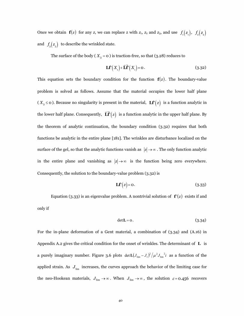
40

Once we obtain ( )zf for any z, we can replace z with z1, z2 and z3, and use f1

z1( ) , f

2z

2( )

and f3

z3( ) to describe the wrinkled state.

The surface of the body ( 03 =X ) is traction-free, so that (3.28) reduces to

L ¢f X1( ) +L ¢f X

1( ) =0 . (3.32)

This equation sets the boundary condition for the function ( )zf . The boundary-value

problem is solved as follows. Assume that the material occupies the lower half plane

( 03 X ). Because no singularity is present in the material, L ¢f z( ) is a function analytic in

the lower half plane. Consequently, L ¢f z( ) is a function analytic in the upper half plane. By

the theorem of analytic continuation, the boundary condition (3.32) requires that both

functions be analytic in the entire plane [181]. The wrinkles are disturbance localized on the

surface of the gel, so that the analytic functions vanish as ¥®z . The only function analytic

in the entire plane and vanishing as ¥®z is the function being zero everywhere.

Consequently, the solution to the boundary-value problem (3.32) is

L ¢f z( ) =0. (3.33)

Equation (3.33) is an eigenvalue problem. A nontrivial solution of ( )z'f exists if and

only if

0det =L . (3.34)

For the in-plane deformation of a Gent material, a combination of (3.34) and (A.16) in

Appendix A.2 gives the critical condition for the onset of wrinkles. The determinant of L is

a purely imaginary number. Figure 3.6 plots ( ) iJJJ2

lim22

1limdet m-L as a function of the

applied strain. As Jlim

increases, the curves approach the behavior of the limiting case for

the neo-Hookean materials, ¥®limJ . When ¥®limJ , the solution e =0.456 recovers

41

the Biot condition for the onset of wrinkles in a neo-Hookean material. When limJ > 169.8 ,

there are two admissible solutions. When limJ = 169.8 , equation (3.34) has a unique

solution 580.0=e . When limJ < 169.8 , equation (3.34) has no solution, i.e. no wrinkles are

predicted by the linear perturbation method.

Figure 3.6 The critical strains for wrinkles are determined by 0=det L . Plotted here are

( ) iJJJ 2limlimdet 22

1 m-L as a function of the applied strain e for different values of limJ . When

∞→limJ , the solution 4560.=e recovers the Biot condition for the onset of wrinkles in a

neo-Hookean material. When 1698.>limJ , Ldet becomes zero at two values of the applied strain.

When 1698.=limJ , 0=det L has a single solution 5800.=e . When 1698.<limJ , ( )Ldet cannot

reach zero at any applied strain.

The critical conditions for the formation of wrinkles obtained by the linear

perturbation analysis are compared with those of creases (Figure 3.5). As Jlim

decreases,

the branch of smaller strains increases, but the branch of larger strains decreases. Observe

that creases always form at a smaller strain than wrinkles. Thus, neither branch of wrinkles

can be realized. Creases, rather than wrinkles, should be observed in the Gent materials.

Once the critical strain is determined by (3.34), the eigenvector is

42

ù

é

-=

ù

é

13113

1

/

1

LLe

e. (3.35)

Consequently, the field of the wrinkled state is determined by f1¢ z

1( ) =w z1( ) and

f3¢ z

3( ) = - L11

/ L13( )w z

3( ) , where ( )zw is an arbitrary scalar-valued function.

3.5 Summary

In this chapter, we study the initiation and development of creases in

strain-stiffening materials. As a result, strain-stiffening effect raises the critical strain for

crease initiation and smoothens creases when the compressive strain is large enough. When

the strain-stiffening effect is strong enough, creases can be completely suppressed. As a

comparison, we also study the initiation of wrinkles in strain-stiffening materials by the

linear perturbation method under Stroh formalism. The classical Stroh formalism is

extended for incompressible materials. Our calculations show that creases always form at a

lower strain than wrinkles, and should be observed.

The stretchability of soft tissues varies with age, pathology, humidity, as well as the

type of tissues. Tendons and ligaments can be uniaxially stretched to a strain of around 15%

[182], cartilage 120% [182], skins 110% [183], and aorta 100% [182]. These values

correspond to Jlim=0.06, 75.2 , 36.2 and 00.2 , respectively. These small values of J

lim

suggests that strain-stiffening effect can play a significant role to suppress the formation of

creasing in these soft tissues.

For polymers, the limiting stretch can be estimated as n , with n being the

number of monomers between two crosslinkers. The value of n can be as small as several or

43

as large as thousands, and limJ can be correspondingly tuned by changing the crosslink

density. The value of limJ can also be tuned by mixing polymers of different kinds. It is

hoped that our theoretical prediction of the smoothening and suppressing of creases can

soon be demonstrated experimentally.

44

Chapter 4

Controlled formation and disappearance of creases

4.1 Introduction

While elastic instabilities, such as buckling of a column or wrinkling of a sheet, have

long been regarded as modes of failure in architectural structures [184], electromechanical

systems [6], and composite materials [7], they have increasingly been exploited for a variety

of applications [13, 20, 22, 27, 28, 81, 185-187]. An example of recent interest is the

formation of surface creases when a soft elastic material is compressed beyond a critical

value [106, 107, 112, 138]. Creases may look superficially like cracks, since both correspond

to sharp, singular features. A significant difference, however, can be readily appreciated and

will have practical implications. While repeated opening and closing of cracks often leads to

fatigue and catastrophic failure, the elastic character of creases makes it possible to cycle a

soft material repeatedly between flat and creased states without inducing damage.

The formation of creases corresponds to a pronounced change of state, reminiscent of

a phase transition. This change of state has recently been used to connect diverse stimuli to

multiple functions. Crease-inducing stimuli include temperature [39], light [136] and electric

fields [134, 188]. Functions enabled by the formation of creases include the control of

chemical patterns [39, 136], enzymatic activity [39], cellular behavior [141], and adhesion

[142]. Each of these applications depends on how creases form and disappear. For a planar

surface under in-plane compression, the creasing instability is supercritical, where creases

45

appear and disappear at the same critical strain, with no hysteresis [107]. In practice,

however, surface tension provides a small energy barrier against creasing, thus leading to

nucleation and growth of shallow, but finite-depth, creases at small over-strains beyond the

critical value [138]. It is tantalizing to imagine devices that exploit snapping creases, in a way

analogous to other snap-through instability used to trigger giant deformation between

bistable states [186, 187]. Unfortunately, the challenges associated with controlling this

barrier, and the related presence of adhesion within the self-contacting creases [138], have

led to widely varying degrees of hysteresis in different material systems [105, 114, 119-121]

complicating the application of creases.

In this chapter, we describe a strategy to create bistable flat and creased states, and to

switch between the two states repeatedly, with hysteresis, at reproducible strains. We

pre-compress a thick substrate, and then attach a thin film on top of the substrate. When we

further compress the substrate-film bilayer, the difference in compression between the two

layers defines an elastic energy barrier that separates the flat state from a state with deep

creases that penetrate into the substrate. We use a combination of experiments and

calculations to show that this approach yields well-defined bistable states, connected by a

snap-through instability. The strains at which the creases form and disappear are tunable

over a large range, through the pre-compression of the substrate and the relative thickness of

the film.

4.2 Subcritical creases

The formation of creases can be either a supercritical or subcritical bifurcation. We

46

sketch the bifurcation diagrams using the applied strain e as the control parameter, and

the depth of crease d as an indicator of state (Figure 4.1). The depth of a crease d is defined

as the distance between the uppermost point on the free surface and the bottom of the

self-contacting region. For each type of bifurcation, a compressed solid has two branches of

equilibrium states: the flat and the creased states. In the bifurcation diagram, the branch of

flat states corresponds to the horizontal axis d = 0, while the branch of creased states

corresponds to a curve with d > 0. In the supercritical bifurcation, the creased branch is a

monotonic function. When e exceeds a critical value eC

, the flat surface forms creases. The

depth of the creases d is infinitesimal initially, and then increases gradually as e increases.

When e is reduced, the creases disappear at the same critical strain eC

, with no hysteresis.

By contrast, in the subcritical bifurcation, the creased branch is not a monotonic function.

When the applied compressive strain exceeds the strain eF

, the flat state becomes unstable,

but no creased state of small depth exists; rather, the flat surface snaps forward to a state

with creases of finite depth dF

. When the applied compressive strain is reduced, the depth

of the creases decreases gradually initially and then, at a finite depth dB

and strain eB

, the

creased surface snaps backward to the flat state. That is, the switching between the flat and

the creased state is hysteretic.

We can also describe the subcritical bifurcation by sketching the change in elastic

energy E to form creases as a function of the depth of the creases d (Figure 4.1c). A

minimum energy corresponds to a stable equilibrium state, and a maximum energy

corresponds to an unstable equilibrium state. The shape of the energy landscape depends on

the applied compressive strain e . At a very small strain, Bee < , creases of any depth raise

47

the energy, and the flat state is stable. At a very large strain, Fee > , the flat state is unstable,

and a creased state is stable. At an intermediate strain, FB eee << , the energy landscape has

two local minima, one corresponding to a flat state, and the other to a creased state. Between

the snap-forward strain eF

and the snap-backward strain eB

lies the Maxwell strain eM

,

at which the two energy minima are equal. The flat state has a lower energy than the

creased state when MB eee << , and the opposite is true when FM eee << .

Figure 4.1 Supercritical and subcritical creases. Bifurcation diagrams for (a) supercritical and (b)

subcritical creases. (c) Energy landscape corresponding to the subcritical bifurcation diagram.

48

Figure 4.2 Experimental setup. A mounting layer is stretched to length 0L , and a substrate of

undeformed thickness sH is attached over the mounting layer. The mounting layer is partially

relaxed to length L, and a film of undeformed thickness fH is attached over the substrate. The

mounting layer is further relaxed to length l.

We design a system capable of tunable hysteresis of creases by using a multilayer

setup (Figure 4.2). We stretch a mounting layer to a length L0, and attach a substrate of

undeformed thickness m 200m=sH . We then partially relax the mounting layer to a length

L , which compresses the substrate to a pre-strain e0= 1-L / L

0. On the pre-strained

substrate we attach a film of undeformed thickness m 4 m=fH . When we relax the

mounting layer to a length l, the film is under a compressive strain of e = 1- l / L . Both the

film and substrate are poly (dimethyl siloxane) (PDMS; Sylgard 184, Dow Corning)

elastomers of the same composition (40 : 1 base : crosslinker by weight), and thus possess

identical elastic properties in the undeformed state (shear modulus G = 16 kPa). The

mounting layer is a much stiffer and thicker PDMS slab ( G = 260 kPa), which keeps the

bottom boundary of the substrate nearly planar while enabling the application of large

compressive strains. All experiments are conducted with the surface submerged under an

aqueous solution containing 0.5 mg/mL 3-[hydro(polyethyleneoxy) propyl]

heptamethyltrisiloxane (Gelest), which greatly reduces both surface tension (to ~ 0.8 mN/m)

and self-adhesion [138], minimizing the importance of these effects compared to elasticity.

49

As a result, the hysteresis arises predominantly from the elastic barrier due to the differential

strain between the thin film and substrate, rather than the small residual surface energy and

adhesion in the self-contacting region.

4.3 Methods

We use a combination of experiments and simulations to realize and study the

subcritical creases, and demonstrate its controllable hysteresis.

4.3.1 Sample preparation

All experiments are performed on bilayers supported on a pre-stretched elastic

‘mounting layer’. The film layer and substrate layer consist of Sylgard 184 (Dow Corning)

PDMS, while the mounting layer is prepared using a custom PDMS formulation from Gelest

Inc. The mounting layer is prepared by first thoroughly mixing part A containing 99.997%

fumed silica reinforced vinyl terminated PDMS (DMS-V31S15, Gelest Inc.) and 0.003%

platinum catalyst (SIP6831.2) and part B containing 90% vinyl terminated PDMS

(DMS-V31) and 10% trimethylsiloxy terminated methylhydrosiloxane-dimethylsiloxane

copolymer (HMS-301) by a weight ratio 3 to 1. The mixture is then degassed, spread onto a

silicon wafer, and cured at 120 °C for 8 h to yield a PDMS film with a thickness of ~1-1.2 mm.

This PDMS film is then cut into 0.8 cm× 2 cm slabs and the shear modulus is determined by

tensile experiments to be 260 kPa. This custom formulation of PDMS provides larger

accessible pre-stretch in the mounting layer (up to 250%) without fracture, while

maintaining a modulus substantially above that of the substrate and film. The substrate layer

50

is prepared by spin coating degassed Sylgard 184 40:1 (by weight) base : crosslinker mixture

onto a polystyrene support at 360 rpm for 120 s. After being cured at 70 °C for 1 h, the

substrate layer is bonded to the mounting layer by spinning coating an adhesive layer of

uncured 40:1 PDMS at 1200 rpm for 120 s and subsequently crosslinking this layer at 70 °C

for 8 h prior to releasing pre-stretch in the mounting layer. Combining the pre-cured film

with the adhesive layer gives rise to the substrate layer with an initial thickness of ~200 µm.

Then the polystyrene is detached and the PDMS substrate layer is put under uniaxial

compression ( 0e ) by partially releasing pre-stretch. The top film is a Sylgard 184 40:1 PDMS

film with a thickness of ~4 µm by spinning at 7000 rpm for 120 s. The top film is first

partially cured at 70 °C for 15 min and then attached to the pre-compressed substrate;

bonding between the layers is achieved by subsequently fully curing the film at 70 °C for 8 h.

The lateral dimensions of the sample are at least 50 times as large as the combined thickness

of the film and substrate, and thus in the central region of the film (where all measurements

are conducted), the stress within each layer should be nearly uniform along the thickness

direction.

4.3.2 Measurement of viscoelastic properties

To measure the viscoelastic properties of our samples, compression stress relaxation

experiments are conducted on Sylgard 184 40:1 PDMS cylinders with 12.5 mm in diameter

and 15 mm in height molded in a syringe by fully curing at 70 °C for 8 h. The compression

stress relaxation experiments are performed on an Instron 5800 compression test machine

with 50 N loading cell by first loading the cylinder to a compressive strain of 0.45 with a

51

strain rate 0.05 min-1, and then tracking the compressive stress relaxation over 1 h while

holding at this strain. Fitting the stress relaxation curve with exponential decay function

gives rise to the characteristic viscoelastic time s 1100= .

4.3.3 Optical and confocal microscope imaging

Over the strains of interest ( 480420 .. -=e for loading and 350480 .. -=e for

unloading), deformation is performed slowly by applying an incremental changes in strain of

~0.01 every 30 min, while the formation/disappearance of creases is monitored in situ using

an upright optical microscope (Zeiss Axiotech Vario) in bright field reflection mode.

Mechanical perturbation is performed with the sample held at a fixed strain by gently poking

the surface with a rounded glass micropipette prepared by pulling a heated glass pipette until

break and then forging the tip with a torch.

For laser scanning confocal microscopy (Zeiss 510 META), the top film is labeled by

incorporating a small amount of fluorescent monomer (4.5 µg fluorescein-o-acrylate per 1 g

PDMS). The sample surface is immersed in a refractive index matched fluid of 72% by weight

glycerol and 28% water [138].

4.3.4 Numerical analysis

We use finite-element software ABAQUS to simulate snapping creases in a bilayer

film-substrate structure subject to uniform external compression with the substrate under

pre-strain. Both the film and the substrate are modeled as incompressible neo-Hookean

materials. We write a user-defined material subroutine UMAT for the substrate to include

52

the pre-strains in the free energy function. In order to break the translational symmetry, a

small defect (10-4 times the total thickness sf HH + in size) is prescribed on the surface,

and a crease will form on the position of the defect when the critical strain is reached. To

eliminate the effect of the defect, its size is set much smaller than the thickness of the film. At

the same time, to resolve the field close to the defect, the size of the elements close to the

defect is made much smaller than the size of the defect. The spacing of the creases is

prescribed as 2.5 times of the total thickness of the film and substrate, which is similar to the

experimental observations. Symmetry is assumed so that only half of a crease is simulated.

Riks method based on arclength continuation is used to solve the boundary value problem so

that not only the stable solutions, but also the unstable solutions can be captured. After the

onset of a crease, the crease tip folds up and forms self-contact. The combination of the Riks

method and contact makes the convergence of the simulation hard. A thick layer with

extremely low shear modulus (1/100 of the film and substrate shear modulus) is added on

the top of the film to prevent self-contact. The top boundary of the extremely compliant layer

is constrained to be flat so that instability cannot form there, but can only form on the

interface between the film and the extremely compliant layer. As shown in [140], when the

modulus of the top layer is much smaller than that of the film and substrate, the result of the

interfacial crease asymptotically approaches that of a surface crease. In order to realize the

uniaxial compression condition as in the experiment by a 2D simulation, we model an

axisymmetric ring under uniaxial compression parallel to the symmetry axis. The radius of

the ring has to be much larger than its thickness so that the curvature of the ring can be

neglected. Element type CAX8H is used.

53

4.4 Results

We use reflected light optical microscopy to obtain top-view images in situ while

relaxing the mounting layer (Figure 4.3a). The substrate is under pre-strain e0=0.15. When

the film is compressed, the flat surface snaps forward into the state of deep creases at a strain

of eF=0.45. Notably, the value of snap-forward strain e

F is very close to the anticipated

value of 0.44, i.e., the critical strain for creasing of the film, since the barrier due to surface

tension here is very low, and hence even small defects are sufficient to enable creases to

nucleate. As compressive strain is further increased, additional deep creases nucleate and

grow on the surface, eventually packing into a quasi-periodic array, as seen in Figure 4.3a,

panel iii. The tendency of creases to adopt an average spacing proportional to the layer

thickness, but without well-defined periodicity, is well known [113], and results from the

difficulty of sliding creases laterally across the surface to adjust the crease locations initially

defined by the nucleation and growth process. Once the quasi-periodic array is established,

further compression causes the crease spacing to be reduced in an affine manner, i.e., such

that the spacing between creases follows ))(( ea -+ 1sf HH . Here, we measure a value of a

that ranges from 1.9-2.8 between neighboring creases. Thus, we adopt a typical value of

52.=a for the numerical simulations. When the compressive strain is reduced below the

snap-backward strain, the surface becomes flat again. No scars or other visible signs of the

creases remain.

54

Figure 4.3 Hysteresis of creases. The substrate is pre-compressed by a strain of 1500 .=e , and the

film-substrate bilayer is then subjected to an additional compressive strain e . (a) Optical microscopy

images show that (i) the surface is flat at 0=e , (ii) snaps into creases at 450.=e , (iii) forms an

array of creases at larger compressive strains, and (iv) becomes flat at 360.=e . (b) Normalized

crease depth as a function of the strain applied to the bilayer. The lines are predictions from the finite

element method, with the solid line being the stable solution and the dashed line the unstable solution.

The dots are experimental results, with the solid dots being on the snap-forward path and the open

dots on the snap-backward path. The inset shows the confocal cross-section at a strain of 460.=e .

(c) Cross-sections (with only the top 2/3 simulation volume shown) generated from finite element

simulation showing the distribution of normalized true stress in the compression direction ( G/112 )

at three different strains: right before snap-forward (a ), right after snap-forward ( ), and right

before snap-backward ( g ), as indicated in (b) with star symbols.

We use finite-element software ABAQUS to simulate the formation of creases. To

construct the entire branch of ceased states, namely, both the stable and unstable

equilibrium states, we use the Riks method of arclength continuation [189]. Due to the

combination of the Riks method and issues associated with self-contact, the simulation often

does not converge. To enable these calculations, we therefore place a much softer material on

top of the film, which prevents surface self-contact and facilitates convergence of the

simulation. As the modulus of this top layer is made much smaller than that of the film and

substrate, the result will asymptotically approach that for a free surface [140]. As an example,

55

we present the bifurcation diagram for the case e0=0.15 and ( ) 020./ =+ fsf HHH

(Figure 4.3b) obtained using this method. Also shown are cross-sections with the contour

plots of the normalized true stress in the compression direction generated from the

simulation (Figure 4.3c). The snap-forward strain is set by the condition to form a crease in

the film, which should be the same as the critical strain for a crease to form in a

homogeneous material under uniaxial compression, eF=0.44

[107]. The result calculated

here,eF=0.46 , is slightly higher than this value, reflecting the small influence of the soft

material placed above the film. We focus on the case that the film is much thinner than the

substrate, sf HH << . The equilibrium depth of this crease will be set by the substrate

thickness—that is Fd is a fraction of sH . Over some intermediate range of strains, two

(meta-)stable states exist, one corresponding to a flat surface ( d =0), and the other to a deep

crease. In this regime, the film remains below the critical strain for creasing, and hence a

shallow crease with d <<Hf raises the elastic energy, while the substrate is above the

critical strain, and hence a deeper crease that penetrates into the substrate with d >>Hf

can lower the elastic energy.

To provide a detailed comparison with these predictions, we use laser scanning

confocal microscopy (LSCM) to characterize the cross-sections of the samples. The film is

stained with fluorescein [138], and the deep crease is clearly visible (Figure 4.3b inset).

Experiments show that upon loading (solid symbols) the surface remains flat until a strain of

450.=e before forming creases. Just beyond this point, a normalized crease depth of

360.)/( =+ fsF HHd is measured, clearly indicating that the creases extend a distance many

times the film thickness into the substrate. These values are in good agreement with

56

numerical predictions. As mentioned above, the snap-forward strain eF

obtained by the

finite element simulations is around 0.46, which is slightly above the anticipated value of

0.44, due to the addition of the extremely compliant layer to help the numerical convergence.

The snap-forward strain 450.=Fe observed in experiments also represents a slight

overestimate due to the small remaining barrier from surface tension.

Upon subsequently reducing the strain (open symbols), the creases become shallower,

reaching a limiting depth of )(. sfB HHd += 120

before undergoing a discontinuous

snap-through transition back to the flat state at value of eB=0.38 . The experimental results

and numerics show good agreement, although the measured values of eB

are slightly lower

than the predictions. In the simulations, the snap back strain eB

is slightly overestimated

due to the soft layer placed above the film. We also suspect that the experimental value of

eB

may be reduced slightly due to a small amount of adhesion of the surface within the

self-contacting region. Nevertheless, bistability between flat and creased states, and a

well-defined window of hysteresis are clearly developed by applying a compressive pre-strain

to a soft substrate underlying a soft film.

Our experimental measurements show that the snap-forward and snap-backward

strains are reproducible (Figure 4.4). The measured values of eF

and eB

remain

unchanged over several cycles within the precision of our measurements, once again

indicating that no permanent scarring or damage to the material has occurred. The inset

images in Figure 4.4 show the first cycle (a and b) and the third cycle (c and d) switching

between creased states and flat states. During the third cycle, the sample is left creased

(image c) for 2-3 days prior to snapping back at the same strain, indicating that even

57

long-term aging does not damage the material. However, the creases do form at the same

locations during each cycle, presumably due to the heterogeneities in the film that

consistently serve as nucleation sites [119].

Figure 4.4 Switching between flat and creased states. The sample is switched between flat and

creased states by cyclically increasing and decreasing the strain. The dots are experimental data. The

dashed lines are the snap-forward strain Fe and snap-backward strain Be calculated using the

finite element method. The optical images show the surface in four states.

Figure 4.5 In the strain range of FM eee << , flat surface is metastable against mechanical

perturbation. (a) When the substrate is subject to a pre-strain of 1500 .=e

and the bilayer is subject

to an additional compressive strain of 420.=e , between the Maxwell strain and the snap-forward

strain, the flat surface is metastable. (b) A gentle poke overcomes the energy barrier and (c) the flat

surface locally snaps into a deep crease. (d) The deep crease propagates at both ends and crosses the

entire surface of the sample over time.

58

Figure 4.6 The zero-speed strain and the Maxwell strain. (a) The speed at which an isolated crease

propagates or retracts is measured experimentally as a function of the applied strain. The interpolated

zero-speed strain is 00503970 .. ±=e , which is close to the Maxwell strain 4020.=Me calculated

using the finite element method (indicated by the red open circle). (b) The energy difference between

creased and flat states as a function of the applied strain is calculated using the finite element analysis.

The Maxwell strain is the strain where creased state has the same energy as flat state (indicated by the

red open circle).

When the applied strain lies between the Maxwell strain eM

and the snap-forward

strain eF

, the flat state is metastable against the formation of creases, and hence it should be

possible to mechanically perturb the surface to overcome the elastic energy barrier and drive

the formation of a deep crease. Figure 4.5 shows just this behavior on the surface of a bilayer

with 1500 .=e and 420.=e gently poked with a glass micropipette. Initially, a crease

59

forms rapidly, and only in the vicinity of the perturbation. However, since the crease is lower

in energy than the flat state, this localized crease spreads laterally, or “channels”, slowly from

both ends over time. While this local snapping is fast, propagation of the short deep crease is

slow. On the contrary, if the applied strain is below eB

, the flat surface is the global energy

minimum and should be stable against perturbations. For bilayer with 1500 .=e and

370.=e , while poking with a glass micropipette induces formation of a transient crease,

the flat state is quickly recovered.

This behavior allows us to experimentally determine the Maxwell strain, where the

crease propagation speed should vanish, which is otherwise difficult to measure. As in Figure

4.5, an isolated crease is formed first by poking the surface of a sample compressed to

eM<e <e

F. The compressive strain is then reduced stepwise and the crease propagation

velocity characterized at each step. As plotted in Figure 4.6a, the growth velocity decreases as

the applied strain is lowered, due to the reduction in the driving force for growth (i.e., the

difference in elastic energy between the flat and creased states), just as in channeling of

cracks [190]. When the strain is reduced to the Maxwell strain, the crease ceases to

propagate, and ultimately begins to retract from both ends with further decreases in strain.

In Figure 4.6b, we plot the normalized energy difference between the creased state and the

flat stated obtained by simulations. The shallow crease solution always has higher energy

than the flat state, while the deep crease solution has energy lower than the flat state when

the strain is higher than the Maxwell strain. The predicted Maxwell strain, defined as the

strain when the flat state and the deep creased state have the same elastic energy, is denoted

by red open circles in Figure 4.6a and 4.6b. When e0=0.15 and 02.0)/( =+ sff HHH , the

60

Maxwell strain is predicted as 4020.=Me , while the measured value is eM=0.397 ±0.005,

very close to the prediction. However, we note that the predicted Maxwell strain is for

periodic creases, while the measured Maxwell strain is for an isolated crease, thus the two

should not agree perfectly. While the kinetics of crease channeling remain under study, we

Figure 4.7 Tunable hysteresis of creases. (a) Snap-forward and snap-backward strains as a function

of pre-strain for different thickness ratios. The black dotted line indicates the relationship

( ) )( 00 1 eeee --= FB between snap-forward strain Fe and snap-backward strain Be , expected in the

limit of vanishing film thickness. (b) Snap-forward and snap-backward crease depths as a function of

pre-strain for different thickness ratios. Dashed lines (snap-forward) and solid lines (snap-backward)

are calculated using the finite element method. The black solid symbols (squares for snap-forward and

circles for snap-backward) are experimental results for thickness ratio ( ) 020.=+ sff HHH , in good

agreement with numerical results.

61

note that the slow propagation speeds of 0.54 mm/s to -0.14 mm/s (Figure 4.6a), likely reflect

the viscoelastic relaxation of material elements near the front of the propagating crease, in a

similar fashion as for propagating cracks [191].

We use finite element simulations to characterize how the hysteresis of creases

depends on the level of pre-strain and the thickness ratio of the film and substrate (Figure

4.7). The snap-forward strain eF

has no dependence on either quantity, as it is simply

determined by the stability of the film against forming a shallow crease. In contrast, the

snap-backward strain eB

increases with Hf

Hf+H

s( ) but decreases with e0. Snapping

back is determined by the difference between the energy reduction in the substrate and the

energy increase in the film in the deep creased state with respect to the flat state. When the

pre-strain e0 is larger, the energy reduction in the substrate in the deep creased state is

bigger and hence the snap-backward strain Be is lower. When 0e is smaller, the

snap-backward strain gets closer to the snap-forward strain Fe and converges to Fe when

00 =e . In the limit of vanishing film thickness, the snap back strain Be should correspond

to the point where the strain in the substrate drops to the critical strain for creasing. This

would lead to the relationship ( ) )( 00 1 eee --= εFB , as plotted in Figure 4.7a (black dotted

line). When the thickness ratio Hf

Hf+H

s( ) is larger, the energy increase in the film in

the deep creased state is bigger and the snap back strain is higher. The snap-forward depth

dF

is primarily set by the thickness and strain of the substrate. Hence, dF

is almost

independent of the film thickness but increases with the pre-strain 0e . However, the snap

back depth dB

increases with the film thickness, for similar reasons as the effect on Be

described above. The snap back depth dB

also increases with the pre-strain 0e , since the

62

depth of the crease increases with the strain in the substrate. With the decrease of 0e , dF

gets closer to dB

. Finally both converge to 0 when 00 =e , and the instability becomes

supercritical with no hysteresis. In the current study, we only consider pre-strains 200 .≤e ,

because larger pre-strains yield wrinkles at strain smaller than eF

. However, we note that

reducing the modulus of the film below that of the substrate allows the pre-strain 0e to be

tuned over a larger range. We also include in Figure 4.7 the corresponding experimental

results for the thickness ratio studied, Hf

Hf+H

s( ) =0.02 , which show rather good

agreement with numerical results. These results provide detailed guidelines for fine-tuning

both the extent of the hysteresis window in strain, as well as the amplitudes of both the

snap-in and snap-out transitions.

4.5 Summary

In this chapter, we have described a robust method for controlling the hysteretic

behavior of surface creases through application of compressive pre-strain to the substrate of

a soft bilayer. Over a well-defined range of strain, the system shows kinetic bistability

between flat and deep creased states with snap-through transitions between these states at

either extreme. Surfaces can be repeatedly snapped forward and backward between these

states with little variation, and in good agreement with the predictions from numerical

analysis. We anticipate that the greatly improved control over hysteresis, and the

demonstration of bistability over a substantial range of strain will open new opportunities

for applications of creases in sensors and responsive surfaces. This experimental system of a

bilayer supported on a pre-stretched foundation provides great freedom to independently

63

tune the modulus, thickness and pre-stretch/compression of both the substrate and film

layers. While the current study has concerned only a very small range of parameter space

with small values of ( )sff HHH + , identical material properties for the film and substrate,

and a narrow range of 0e , we anticipate that the same approach will enable detailed studies

of the rich landscape of behaviors in other regimes.

64

Chapter 5

Creases on the interface between two soft materials

5.1 Introduction

Bonded materials with dissimilar properties are ubiquitous. They exist in composite

materials [192], geological strata [193, 194], electronic devices [195], biological tissues [44,

196] and soft actuators [197]. In many cases, stresses arise due to differences in thermal

expansion [198-200], chemical reactions [201], growth [44, 52], swelling [118], or

mechanical pre-strains [202]. Such mismatches may cause buckling instabilities [7, 192, 200,

203], which can reduce the strength of structures [7, 192, 200, 203] and lead to debonding of

the interfaces [198, 199, 204].

Interfacial instability has long been regarded as a bifurcation from a state of flat

interface [7, 192, 200, 203]. For example, Biot [100, 205] studied two elastic materials

compressed along a direction parallel to the interface. He predicted that the interface forms

wrinkles at a critical compression, similar to the formation of wrinkles on the free surface of

a soft solid [97]. These wrinkles have dynamic analogs: Stoneley waves on the interface

between two materials [100, 206-208], and Rayleigh waves on the surface of a homogeneous

material [208-210]. Wrinkles, however, have not been observed on surfaces of homogeneous

elastic materials under compression; rather, creases have been observed [105, 112-114, 118].

A recent theory shows that surface wrinkles and surface creases are two types of instability,

and the critical strain for the onset of surface wrinkles is higher than that for the onset of

65

surface creases [106]. Notably, these phenomena occur at rather large compressive strains.

While hard elastic materials generally cannot be loaded to such large strains without fracture,

soft materials such as gels and elastomers can easily be compressed to the point of

instability.

Motivated by this recent understanding, in this chapter we reconsider the stability of

the interface between two soft materials. Our theory and experiment show an analogous

localized, large-strain instability, which we call interfacial creases (Figure 5.1). Wrinkles and

creases are two types of bifurcation from the state of flat interface. While wrinkles bifurcate

by a deformation nonlocal in space and infinitesimal in amplitude, creases bifurcate by a

deformation local in space and large in amplitude. In this regard, the wrinkling instability is

of the same type as buckling of columns and plates, while the creasing instability is

reminiscent of cracking, cavitation, shear banding, and phase transformation. Upon

initiation, an interfacial crease corresponds to a field scaled by a single length scale. The

critical strain is independent of this length scale and is scale-free. We calculate the critical

conditions for the onset of the interfacial creases and find that, just like their surface

counterparts, interfacial creases always form at lower compression than interfacial wrinkles.

We show that interfacial creases are V-shaped. The presence of two materials prevents the

interface from self-contact, but the tip of an interfacial crease is singular. Because the

interface does not enter self-contact, the analysis of interfacial creases is simplified

compared to that of surface creases. We demonstrate the existence of interfacial creases by

experiments with hydrogels. By using differential swelling of two types of gels, we can form

interfacial creases and surface creases independently.

66

Figure 5.1 Materials A and B are bonded to each other along a flat interface. Subject to a compressive

strain, the interface may either remain flat (a), or form creases (b).

5.2 Analysis and simulations

5.2.1 Interfacial creases under applied strain

We study the initiation of interfacial creases by comparing two states of equilibrium

subject to the same applied strain (Figure 5.1). In the state of flat interface, the field in either

material is homogeneous, and the elastic energy of the state is denoted by 0U . In the creased

state, one point of the interface is prescribed with a downward displacement L, and the

elastic energy of the state is denoted U. The magnitude of the displacement L is arbitrary, so

long as it is much smaller than any other length in the boundary-value problem (e.g., the

thickness and width of the block used in computation). Once L is prescribed, the creased

state is determined by a boundary-value problem of large deformation. The two states of

equilibrium differ by a deformation of large amplitude, but the difference is localized in a

small region scaled by the length L. The two materials are taken to be incompressible and

neo-Hookean, with shear moduli GA

and GB

. We begin with the case that pre-strains are

absent, and the block is compressed to reduce its width under plane strain conditions. The

applied strain e is defined as the reduction in the width of the block divided by the width of

A

B

(a) (b)

A

B

L

67

the block in the undeformed state. Dimensional considerations dictate that the energy of the

creased state should differ from that of the flat state by

( )ABB GGfLGUU /,20 e=- . (5.1)

As indicated, the dimensionless number f is a function of the applied strain and the ratio of

the shear moduli. The scaling relation (5.1) generalizes the result for surface creases [107].

Without loss of generality, we assume that GA<G

B. We expect that interfacial

creases form by growing into the stiffer material (B). In the absence of applied strain, the

energy of the state of flat interface vanishes, but the energy of the creased state is positive, so

that the state of flat interface is stable. When a sufficiently large compressive strain is applied,

the crease elongates the interface, so that the crease reduces energy in material B, but

increases energy in material A. Because GA<G

B, the crease can reduce the total elastic

energy in the two materials. For a fixed ratio GB

/GA, the function f e,G

B/G

A( ) decreases

monotonically with the applied strain e . An interfacial crease sets in when the creased state

has the same energy as the flat state, namely,

f e,G

B/G

A( ) =0. (5.2)

This condition gives the critical strain for the onset of interfacial crease, ec, as a function of

the modulus ratio, GB

/GA

.

The critical condition (5.2) for the onset of interfacial crease is independent of any

length scale. This scale-free behavior results from two considerations. First, the prescribed

displacement L is assumed to be small compared to other lengths in the boundary-value

problem, such as the thickness and width of the block used in the calculation. The flat state

differs from the creased state by a deformation localized within a region scaled with L.

68

Consequently, only the length L enters (5.1), and no length appears in the critical condition

(2). Second, the theory of elasticity does not have any material-defined length scale. The

situation would be different if we accounted for the interfacial tension g between the two

materials. The interfacial tension, together with the elastic modulus G, would provide a

length scale, the elastocapillary length g /G . This length scale can vary across many orders

of magnitude depending on the material system, but typical values for elastomer/elastomer

interfaces are g ~ 1 – 10 mN/m and G ~ 100 kPa, while for gel/gel interfaces they are g ~

0.1 – 1 mN/m and G ~ 10 kPa, in both cases yielding g /G ~ 10 – 100 nm. Incorporating

interfacial tension will cause the tip of an interfacial crease to be rounded on a length scale of

g /G , rather than being infinitely sharp. Interfacial tension would also provide a barrier

against the initiation of interfacial creases, just as in the case of surface creases, thus

requiring the application of a small amount of overstrain to drive crease nucleation [138].

For simplicity, however, we ignore here the effects of interfacial tension and consider only

elastic contributions, which is appropriate for understanding fully formed creases for

samples much thicker than g /G .

In the above description, the creased state is determined by a boundary-value

problem of large deformation, and the prescribed displacement L specifies the length scale.

This particular way of specifying a length scale, however, does not affect the critical strain for

the onset of the crease. Upon initiation, the creased state is scaled by one length,

independent of how the length is specified.

We use the finite element software ABAQUS to solve the boundary-value problem of

the creased state, from the reference state of flat interface to the current state of a prescribed

69

displacement L (Figure 5.2). Analysis of this type has also been used in our previous work on

surface creases [107]. Due to symmetry, only half of a crease is simulated. The materials

deform under plane-strain conditions, and element type CPE4H is used. Compare the

creased state and the flat state subject to the same applied strain e . Their energy difference

0UU - is plotted as a function of the applied strain e for a fixed value of the modulus ratio

5=AB GG / . When e <0.512, the state of flat interface has a lower elastic energy than the

creased state. When e >0.512, the state of flat interface has a higher elastic energy than the

creased state. The strain ec=0.512 is identified as the critical condition for the onset of the

interfacial crease.

Figure 5.2 The energy difference between the creased state U and the flat state 0U plotted as a

function of the applied strain e for a fixed value of the modulus ratio 5=AB GG / . When 5120.=e ,

the energy of the creased state is equal to the energy of the flat state, and 5120.=e is identified as

the critical condition for the onset of the interfacial crease.

We use another finite element method to simulate the growth of an interfacial crease

(Figure 5.3). In the reference state, two materials A and B are bonded with a flat interface

(Figure 5.3a). We make use of the symmetry condition, and only simulate the right half of a

crease. After a crease initiates, its growth does depend on the size of the block used in the

calculation. Here the two materials in the reference state have the same thickness H, and the

70

lateral size of the simulation box (corresponding to half of the spacing between creases) is set

to be W =H , close to what is observed in our experiments. To seed the crease, a small

defect is prescribed on the left end of the interface. The size of the defect is much smaller

than the thickness of either material, but is large compared to the size of the surrounding

mesh. An image of a region in the vicinity of the defect, with depth D and angle a , is shown

in Figure 5.3b. In the current state, a horizontal displacement is applied on the boundary on

the right (Figure 5.3c). The top and bottom boundaries are constrained to remain planar, so

that they cannot form surface creases. The boundary on the left is a plane of mirror

symmetry. The two materials are compressed in the horizontal direction and expand in the

vertical direction, while the depth of the crease, L, evolves as a function of the applied

displacement.

The depth of the crease is plotted as a function of the applied strain (Figure 5.4). The

depth of the crease remains nearly zero below the critical strain, and begins to grow when the

applied strain is beyond the critical value about 5120.=ce . The crease is seeded with defects

of different depths D and angles a . Meshes with different size are used as well: mesh 1 uses

18 elements along the defect; mesh 2 uses 36 elements along the defect. So long as a defect is

small compared to the thickness of each material, but large compared to the size of

surrounding mesh, the depth and the angle of the defect and the mesh size have a negligible

effect on the critical strain for the onset of the crease and subsequent growth of the crease.

71

Figure 5.3 Finite element model. (a) In the reference state, two materials A and B are bonded with a

flat interface. A small defect is prescribed on the left end of the interface. (b) An image of a region in

the vicinity of the defect, with depth D and angle a . (c) In the current state, the two materials are

compressed in the horizontal direction and expand in the vertical direction, while the depth of the

crease, L, evolves as a function of the applied displacement.

Figure 5.4 The depth of the crease is plotted as a function of the applied strain. The crease is seeded

with defects of different depths D and angles a . Mesh 1 uses 18 elements along the defect, and mesh

2 uses 36 elements along the defect.

The elastic energy is a function of the applied strain (Figure 5.5). Let 0U be the

eL

(c) Current state (b) Close-up of defect

a D

(a) Reference state

A

B

H

W

defect

H

72

energy in the two materials in the state of flat interface, and FU be the energy in the two

materials calculated by using the finite element method of simulating crease growth. When

the applied strain 5120.<e , the interface remains flat, and the total elastic energy is the

same as that in the two materials in the state of flat interface 0UU F / = 1. When 5120.>e ,

a crease forms, reducing the total elastic energy below that in the two materials in the state of

flat interface, 0UU F / < 1. Consequently, we identify 5120.=e as the critical strain for

the onset of creases, which is consistent with the result by the method of prescribing a length

scale (Figure 5.2). After an interfacial crease forms, the elastic energy of the bottom material

UB

decreases while the elastic energy of the top material UA

increases. Since the bottom

material is stiffer than the top material, the decrease in elastic energy of the bottom material

is larger than the increase in the energy of the top material. Consequently, the interfacial

crease reduces the total energy FU .

Figure 5.5 Energy in both materials, FU , energy in material A, AU , and energy in material B, BU

are plotted as functions of the applied strain. Each energy is normalized by the energy in the two

materials in the state of flat interface, 0U .

73

Figure 5.6 Interfacial creases under applied strain. (a) The critical strain for the onset of creases as a

function of the ratio of the shear modulus, AB GG / . Also plotted is the critical strain for the onset of

wrinkles. (b) The depth of a crease as a function of the applied strain for several values of AB GG / .

(c) Shapes of creased interfaces at applied strain 550.=e , for several values of the modulus ratio.

Similarly, we can simulate the initiation and growth of interfacial creases for other

modulus ratios. As expected, the critical strain for the onset of interfacial crease decreases as

the modulus ratio GB

/GA increases (Figure 5.6a). In the limit G

B/G

A®¥ , the critical

(b)

(c)

(a)

74

strain for the onset of an interfacial crease recovers that of a surface crease, ec=0.354 [106,

107]. In the limit GB

/GA® 1 , the two materials are elastically homogeneous, and an

interfacial crease will not form under any compressive strain, so that ec® 1. Also plotted in

Figure 5.6a is the critical strain for the onset of interfacial wrinkles. While the onset of

interfacial creases is determined by a boundary-value problem of large deformation, the

onset of interfacial wrinkles is determined by a boundary-value problem of infinitesimal

deformation superimposed on a known large deformation [100, 205]; see Section 5.3 for

more details. For any value of modulus ratio, the interfacial crease sets in at a critical strain

lower than the interfacial wrinkles.

Figure 5.6b shows the evolution of interfacial crease depth with the applied strain for

different modulus ratios. The limit GB

/GA®¥ corresponds to a surface crease. At a lower

value of GB

/GA, material A retards the onset of the crease, and the interfacial crease is

shallower than the surface crease under the same applied strain. The calculated shapes of the

creased interfaces are V-shaped (Figure 5.6c). Under the same strain 550.=e , the

interfacial crease is deeper for a larger value of GB

/GA

, and asymptotically approaches the

shape of a surface crease with self-contact as ¥®AB GG / .

5.2.2 Interfacial creases under both applied strain and pre-strains

We next study interfacial creases under both pre-strains and applied strains (Figure

5.7). Prior to bonding, material B is subject to pre-stretches l1

pre and l2

pre , while material A

is undeformed (Figure 5.7a, b). The pre-stretches are defined as the current length divided by

the original length, with subscripts 1 and 2 indicating the coordinate directions in the plane

75

of the interface. After bonding, both materials are subject to applied stretches l1 and l

2,

which can be controlled independently of the pre-stretches l1

pre and l2

pre (Figure 5.7c).

Both materials are taken to be incompressible, l1

prel2

prel3

pre = 1 and l1l

2l

3= 1 .

Figure 5.7 Two materials with bonding on the interface under both pre-strains and applied strains.

(a) In the unbonded state, both materials are stress-free. (b) In the bonded state, material B is subject

to pre-stretches pre1l , pre

2l and pre3l , and material A is stress-free. (c) In the loaded state, the

bilayer is subject to applied stretches 1l , 2l and 3l .

For the same reason stated above, the energy in the creased state differs from that in

the flat state by U -U0=G

BL2 f , but f now depends on five dimensionless parameters:

ABprepre GG / , , , , 2121 llll . A further analysis, however, indicates that the critical condition for

the onset of interfacial creases depends on three combined parameters:

022121 =

pre

ABprepre GGf lllll /,, . (5.3)

This result is obtained as follows.

In analyzing creases, we assume that the materials deform under the generalized

plane strain conditions (Figure 5.7c). The deformation gradient is invariant with respect to

axis 2 and takes the form

BpreL11l

BpreL22l

BpreL33l

AL1

AL2AL3

(a) Unbonded state (c) Loaded state (b) Bonded state

BpreL333ll

AL1

AL2

AL3

A

BL1

BL2

BL3

B BpreL111ll

BpreL222ll

AL22l AL33l

AL11l

76

ù

é

=

3331

2

1311

0

00

0

FF

FF

lF . (5.4)

The free energy density of material A is

WA=

GA

2F

iKF

iK+

GA

2l

2

2 . (5.5)

Each repeated index implies a sum over 1 and 3. Consider an intermediate state in which

material A is stretched along the three axes by l2

-1/2 ,l2,l

2

-1/2( ) . Using this intermediate state

as a new reference state, the deformation gradient in the plane of axes 1 and 3 is F̂iK= l

2

1/2FiK

.

Rewrite the free energy density as

WA=

GA

2l2

F̂iK

F̂iK+

GA

2l

2

2 . (5.6)

The free energy density in material B is

WB=

GB

2F

iKF

Ka

preFiL

FLa

pre +G

B

2l

2l

2

pre( )2

. (5.7)

Write F̂Ka

pre = l2

pre( )1/2

FKa

pre , so that

WB=

GB

2l2l

2

preF̂

iKF̂

Ka

preF̂iL

F̂La

pre +G

B

2l

2l

2

pre( )2

. (5.8)

Because 2l and pre2l are prescribed constants, the last terms in (5.6) and (5.8) do not

contribute to the energy difference between the creased state and the flat state. The first

terms in (5.6) and (5.8) describe the energy change from the intermediate states to the

current states, with plane strain deformation F̂iK

in material A and plane strain

deformation and pre-stretches preKiK FF a

ˆˆ in material B. Consequently, the deformation under

generalized plane strain conditions correspond to the deformation under plane strain

conditions, with the effective shear moduli 2/ lAG and preBG 22/ ll for the two materials.

Thus we show that the critical condition for the onset of creases depends on three

77

dimensionless parameters: preAB

prepre GG 22121 lllll /,, . This result generalizes the critical

condition for the onset of surface creases [107]. The same conclusion holds for the critical

condition for the onset of wrinkles. Similar combinations of parameters have been identified

in an independent analysis of wrinkles in film-substrate structures [170].

The critical condition for the onset of interfacial creases is calculated using finite

element method. We write a user-defined material subroutine UMAT to include the

pre-stretches in the free energy function. For a given value of GB

/GAl

2

pre , the critical

condition is represented by a curve in the plane spanned by parameters l1l

2 and

l1

pre l2

pre

(Figure 5.8a). Below the curve interfacial creases form, and above the curve

interfacial creases do not form. The condition for the onset of surface creases corresponds to

the limit GB

/GAl

2

pre ®¥. The critical condition for the onset of wrinkles is plotted in a

similar diagram (Figure 5.8b); see Section 5.3 for details. For a given value of GB

/GAl

2

pre ,

the curve for interfacial creases always lies above the one for interfacial wrinkles. This result

predicts that interfacial creases will form, rather than interfacial wrinkles.

Figure 5.8 (a) The critical condition for the onset of interfacial creases. (b) The critical condition for

the onset of interfacial wrinkles.

(b) (a)

78

5.3 Linear perturbation analysis for the onset of interfacial wrinkles

We calculate the critical condition for the onset of interfacial wrinkles by using the

small-perturbation method described by Biot [100, 205]. Additional results are obtained

here to account for pre-stretches. The analysis relies on the theory of finite deformation of an

elastic body. The reference state is taken to be the bonded state, where the bottom material is

pre-stretched, while the top material is undeformed (Figure 5.7b). Label a material particle

in the body by its coordinate X when the body is in the reference state. In the deformed state,

the material particle moves to a place of coordinate x. The function x X( ) describes the

deformation of the body. The deformation gradient is

FiK=¶x

iX( )

¶XK

. (5.9)

The nominal stress siK

satisfies the conditions of equilibrium

¶s

iK

¶XK

=0. (5.10)

The interface between materials A and B coincides with the plane X3=0 . Across the

interface, both the displacement and traction are continuous:

xi

A = xi

B, (5.11)

si3

A = si3

B . (5.12)

Each material is characterized by the Helmholtz free energy as a function of the

deformation gradient, W F( ) . The nominal stress relates to the deformation gradient by

siK=¶W F( )¶F

iK

. (5.13)

The materials are taken to be incompressible:

79

det F( ) = 1 . (5.14)

The materials are described by the neo-Hookean model. For material A, the free energy is

WA

F( ) =G

A

2F

iKF

iK- det F-1( )P, (5.15)

where P is the Lagrange multiplier used to enforce incompressibility. In general the

Lagrange multiplier is inhomogeneous, and should be solved as a part of the problem. The

material model (5.13) becomes

siK

A =GAF

iK-PH

iK, (5.16)

where H =F-T . In the reference state (Figure 5.7b), material B is pre-stretched to a

homogeneous state with deformation gradient:

F pre =

l1

pre 0 0

0 l2

pre 0

0 0 l3

pre

é

ù

. (5.17)

The material B is also taken to be incompressible, detF pre = l1

prel2

prel3

pre = 1 . For material B,

the net deformation gradient between the current state and the undeformed state is FiK

FKa

pre ,

and the free energy is

WB=

GB

2F

iKF

Ka

preFiL

FLa

pre - detF-1( )P . (5.18)

The material model (5.13) becomes

iKiLpre

Lpre

KBBiK HFFFGs P-= aa . (5.19)

We next perturb from the state of finite deformation (Figure 5.7c), of displacement

( )X0ix , deformation gradient ( )X0

iKF and nominal stress ( )X0iKs . In particular, the

deformation gradient of this state is prescribed by the applied stretches:

ù

é

=

3

2

1

0

00

00

00

l

l

l

F . (5.20)

80

The corresponding field of displacement is XFx 00= . This state of finite deformation is then

perturbed by a state of infinitesimal deformation x X( ) . We write the perturbed state as

( ) ( )XxXxx ~0 += . The other fields are similarly perturbed. Both state ( )Xx0 and the state

( ) ( )XxXx ~0 + satisfy the same governing equations (5.9)-(5.19). Equations (5.9)-(5.12)

reduce to equations for the fields of perturbation:

FiK=¶ x

iX( )

¶XK

, (5.21)

0~

=¶

¶

K

iK

X

s, (5.22)

Bi

Ai xx ~~ = , (5.23)

Bi

Ai ss 33

~~ = . (5.24)

The condition of incompressibility (5.14) is perturbed as

0~0 =iKiK FH , (5.25)

where T

FH-

= 00 . Expanding (5.16) in the Taylor series at 0F and keeping only the linear

term, we obtain that

( ) P-P+=~~~ 0000

iKjLjKiLKLijAA

iK HFHHGs . (5.26)

Similarly perturbing (5.19), we obtain that

( ) P-P+=~~~ 0000

iKjLjKiLijpre

Lpre

KBB

iK HFHHFFGs aa . (5.27)

Inserting (5.21), (5.26) and (5.27) into (5.22), we obtain that

( ) ( ) ( )0

~~0

2

000 =¶

P¶-

¶¶

¶P+

K

iK

LK

j

jKiLKLijAX

HXX

xHHG

XX , (5.28)

( ) ( ) ( )0

~~0

2

000 =¶

P¶-

¶¶

¶P+

K

iK

LK

j

jKiLijpre

Lpre

KBX

HXX

xHHFFG

XXaa , (5.29)

for material A and B respectively. For a given field ( )X0ix , (5.25), (5.28), and (5.29) define a

81

set of linear, homogeneous partial differential equations for the fields of perturbation,

xi

X( ) and P X( ). The displacement and the traction are continuous across the interface.

Consequently, the fields of perturbation xi

X( ) and P X( ) are governed by an eigenvalue

problem. The characteristic equation of this eigenvalue problem defines the critical condition

for the onset of wrinkles. Following an analysis similar to that of Biot [100, 205], we obtain

the critical condition for the onset of interfacial wrinkles:

.011

1111

2

11

33

1

32

33

11

3

12

11

33

1

32

=

ù

é

--

--

ù

é

++

+

ù

é

++

+

pre

pre

B

Apre

pre

pre

B

Apre

pre

pre

B

Apre

G

G

G

G

G

G

ll

ll

l

ll

ll

ll

l

ll

ll

ll

l

ll

(5.30)

This condition is plotted in Figure 5.8b. When l1

pre = l2

pre = l3

pre = 1 , the condition recovers

Biot’s solution [100, 205], and is plotted in Figure 5.6a.

5.4 Experimental results

We perform experiments to show the existence of interfacial creases. In one

experiment, two hydrogels are confined between glass slides (Figure 5.9). The two gels are

bonded to each other, but are not bonded to the glass slides. The colored gel is stiffer than

the colorless gel. The former has a polymer network containing fixed charges, while the latter

has an uncharged network (Figure 5.9a). After preparation, the two gels are nearly

stress-free, and the interface is flat (Figure 5.9b). When placed in water and allowed to swell,

the charged gel is subject to compressive stress due to its inability to expand laterally,

leading to the formation of interfacial creases (Figure 5.9c). The uncharged gel swells

negligibly, so that the top surface does not form surface creases.

82

Figure 5.9 Creases formed on the interface between two hydrogels. (a) A schematic of the

experimental setup. Confined in a 1 mm thick glass slit are two gels, one with a charged network and

the other with unchanged network. The gels are bonded to each other, but are not bonded to the glass.

(b) After the preparation, the two hydrogels are relatively dry and stress-free, and the interface is flat.

(c) When soaked in water, the charged gel swells much more than the uncharged gel, so that creases

form on the interface between the two gels, but not on the free surface of the uncharged gel.

A second experiment is performed to compare interfacial creases and surface creases

(Figure 5.10). A charged gel of thickness H2 = 6 – 8 mm is attached on a glass substrate. A

portion of the gel is then covered with an uncharged gel of thickness H1 = 76 mm (Figure

5.10a). When immersed in a phosphate buffered saline solution containing 274 mM sodium

chloride, both gels swell slightly and generate in-plane equi-biaxial compressive stresses, but

the compression is insufficient to cause either surface or interfacial creases. Deionized water

is then added drop by drop to reduce the concentration of the saline solution, so that the

charged gel swells more and the uncharged gel swells negligibly (as characterized by

fluorescence confocal microscopy). When the swelling ratio of the charged gel reaches

H2¢ H

2=2.4±0.1 , the uncovered portion of the charged gel forms surface creases, while the

interface between the two gels remains flat (Figure 5.10b, d). This critical swelling ratio for

the onset of surface creases is in good agreement with previous reports [112]. When the

swelling ratio is increased to ¢¢H2

H2= 3.3±0.1 , the covered region of the gel forms interfacial

creases (Figure 5.10c, e). At the same degree of swelling, the interfacial creases are shallower

than surface creases, as shown by the cross-sectional confocal images in the insets of Figure

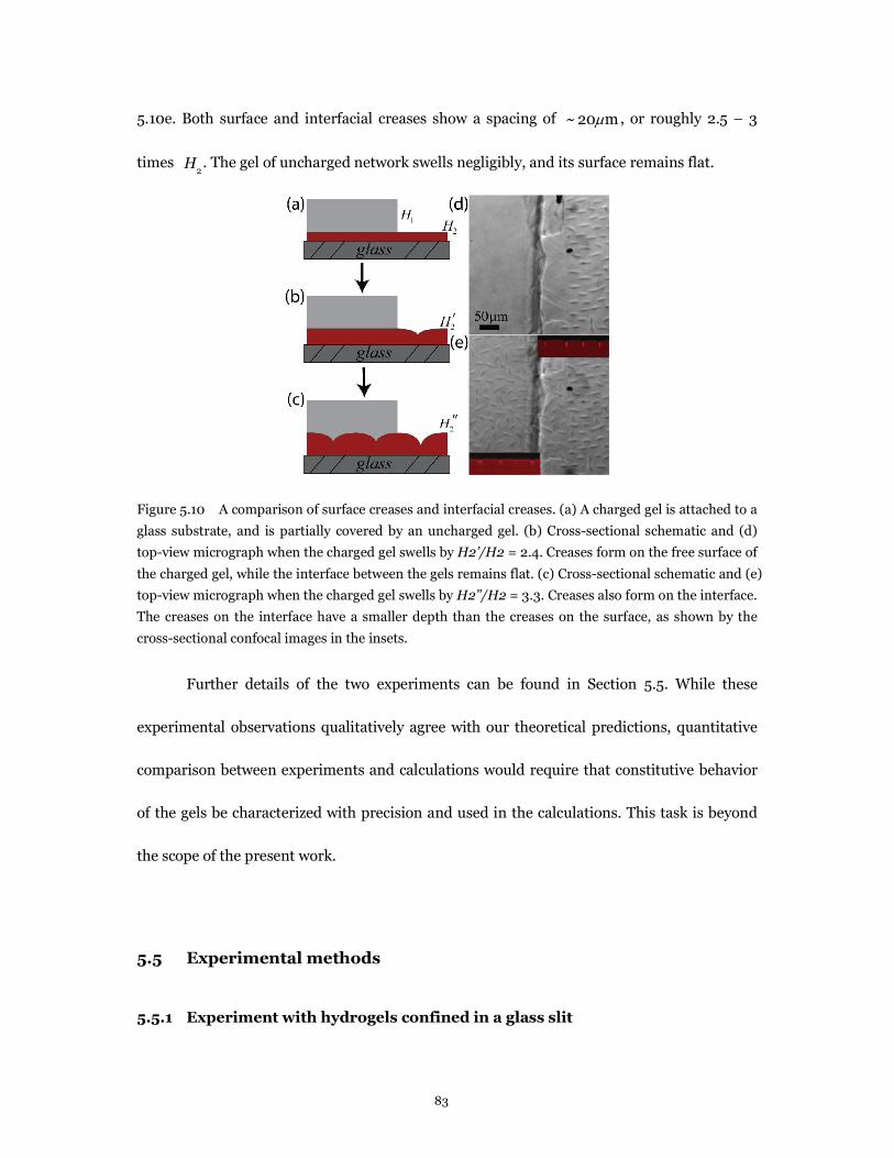
83

5.10e. Both surface and interfacial creases show a spacing of ~ 20mm , or roughly 2.5 – 3

times H2. The gel of uncharged network swells negligibly, and its surface remains flat.

Figure 5.10 A comparison of surface creases and interfacial creases. (a) A charged gel is attached to a

glass substrate, and is partially covered by an uncharged gel. (b) Cross-sectional schematic and (d)

top-view micrograph when the charged gel swells by H2’/H2 = 2.4. Creases form on the free surface of

the charged gel, while the interface between the gels remains flat. (c) Cross-sectional schematic and (e)

top-view micrograph when the charged gel swells by H2’’/H2 = 3.3. Creases also form on the interface.

The creases on the interface have a smaller depth than the creases on the surface, as shown by the

cross-sectional confocal images in the insets.

Further details of the two experiments can be found in Section 5.5. While these

experimental observations qualitatively agree with our theoretical predictions, quantitative

comparison between experiments and calculations would require that constitutive behavior

of the gels be characterized with precision and used in the calculations. This task is beyond

the scope of the present work.

5.5 Experimental methods

5.5.1 Experiment with hydrogels confined in a glass slit

84

A glass slit, thickness 1 mm and width 28 mm, is constructed by gluing glass slides

together (Figure 5.9). The inner surfaces of the slit are treated with trimethylchlorosilane to

reduce adhesion of the gels to the glass surfaces. A charged gel layer is first prepared by

loading the slit with an aqueous pre-gel solution containing 700 mM N-isopropyl-acrylamide,

660 mM sodium acrylate and 45 mM N,N’-methylenebisacrylamide. Gelation is initiated by

adding 1 µL of 10% w/w ammonium persulfate aqueous solution as the initiator and 0.3 µL

N,N,N’,N’-tetramethylenediamine as the catalyst into 200 µL of freshly degassed pre-gel

solution immediately prior to loading the chamber. To stain the charged gel, a small amount

(3.2×10-5 mmol) of a Rhodamine B-labeled methacrylate is incorporated into the 200 µL

pre-gel solution. Next, a softer uncharged gel is prepared on top of the charged gel using the

same procedure as above, but with a pre-gel solution containing 701 mM acrylamide and 19

mM N,N’-methylenebisacrylamide. Some interpenetration of the second gel into the existing

charged gel does occur, and helps to bond the materials together, but based on the relatively

rapid speed of gelation (~ 20 min), this length-scale is small compared to the ~ 1 cm

dimensions of the gels. The contrast in modulus between the gels is not known, but based

simply on the relative crosslinker concentrations, the charged gel should be at least ~

2.4-fold stiffer than the uncharged gel [211]. Following gelation, this confined gel sample is

soaked in deionized water for 3 weeks to reach swelling equilibrium, and the shape of the

interface is recorded using a digital camera.

5.5.2 Experiment with thin layers of gels on a glass substrate

This experiment uses a photo-crosslinkable poly(N-isopropylacrylamide-co-sodium

85

acrylate-co-acrylamidobenzophenone) polymer described in previous reports [112, 212]. A

glass cover slip substrate is pretreated with [3-(methacryloxy)-propyl]trichlorosilane to

provide covalently anchoring, and then a copolymer film is solution cast from chloroform to

yield a film thickness of mH m862 -= , followed by crosslinking by exposure to 365 nm UV

light. A much softer uncharged gel is next formed by loading a freshly prepared de-gassed

aqueous pre-gel solution (containing 701 mM acrylamide and 19 mM

N,N’-methylenebisacrylamide; prepared as above) between the substrate-attached

photo-crosslinked polymer film and a clean cover slip, and allowing 20 min for

polymerization to proceed. The uncharged gel film thickness mH m761 = is defined using

Kapton 300HN films (DuPont) as spacers. To prevent swelling of the photo-crosslinked

poly(N-isopropylacrylamide) film by the pre-gel solution, the neutral gel is formed at 70 °C.

Following polymerization, the cell is cooled to room temperature and the glass slides are

separated. The surface-attached gel bilayer is then transferred to a phosphate buffered saline

swelling solution containing 274 mM sodium chloride. Deionized water is then added

drop-wise to dilute the swelling solution and thus increase the swelling ratio of the charged

gel, while the formation of creases is monitored in situ using either an upright optical

microscope (Zeiss Axiotech Vario) in reflected-light differential interference contrast mode

or a laser scanning confocal fluorescence microscope (Zeiss). Based on a previous report, we

estimate the Young’s modulus of the uncharged gel to be ~ 5 kPa [213], while that of the

charged gel is estimated to be several hundred kPa based on the density of

photo-crosslinking groups in the copolymer.

86

5.6 Summary

We present calculations and experiments to show that an interface between two soft

materials under compression can form creases. A creased state deviates from a state of flat

interface by a deformation large in amplitude and local in space. The critical condition for

the onset of interfacial creases is scale-free. This critical condition is calculated in terms of

elastic moduli, pre-stretches and applied stretches by allowing deviation from a flat state

with a large deformation. By contrast, a wrinkled state deviates from a state of flat interface

by a deformation infinitesimal in amplitude and nonlocal in space. The critical condition for

the onset of interfacial wrinkles is calculated by a small-perturbation method. In all cases

studied, the critical conditions for the onset of interfacial creases are reached before those for

the onset of interfacial wrinkles.

87

Chapter 6

The formation of wrinkles or creases in bilayers

6.1 Introduction

Soft materials, such as elastomers, gels and living tissues, are often under

compression due to forces, swelling, and growth. When the compression exceeds some

critical strain, the soft materials undergo elastic instability, forming, e.g., wrinkles and

creases [3, 10, 12]. Elastic instability of various kinds has been used in engineering to

fabricate stretchable electronics [13], measure material properties [22], tune adhesion [31,

32], change wettability [35], and control surface chemistry [39]. Wrinkles and creases also

provide forms and functions in nature, such as formation of fingerprints [50], invagination

of embryos [51], development of guts [52], folding of brains [56-58] and morphogenesis of

viruses [64] and plants [65-72].

Wrinkles and creases are two distinct types of instability [106]. Wrinkles deviate from

the flat state by a field of infinitesimal strain in a finite region, whereas a crease deviates

from the flat state by a field of large strain in an infinitesimal region (Figure 6.1). To

determine the critical strain for the onset of wrinkles, a field of infinitesimal strain is

superimposed upon the flat state [78, 85, 97, 103]. This superimposed field linearizes the

field equations around the flat state of finite deformation, leading to an eigenvalue problem.

By contrast, the critical strain for the onset of a crease cannot be determined by linearization

around the flat state, but can be determined by allowing the surface to form a localized

88

region of self-contact.

Engineering systems and living tissues often involve layered materials of dissimilar

elastic moduli [52, 56, 57, 214-216]. Several special cases have been well studied. For a stiff

thin film on a compliant thick substrate, the critical strain for the onset of wrinkles is smaller

than that for the onset of creases, and wrinkles are observed in experiments [3, 10, 12, 76, 81].

For a homogeneous material, the critical strain for the onset of wrinkles is larger than that

for the onset of creases, and creases are observed in experiments [105-107, 112-114, 118, 127,

130]. For layered materials of comparable thicknesses and moduli, the critical strain for the

onset of wrinkles can be either smaller or larger than that for the onset of creases [99, 122,

170-172]. It is tempting to expect a layered material to form wrinkles if the critical strain for

the onset of wrinkles is smaller than that for the onset of creases, or vice versa.

This expectation turns out to be wrong. In many cases, the bifurcation points

themselves do not predict the behavior of a layered material. Rather, we need to construct

bifurcation diagrams. We illustrate our findings using bilayers of dissimilar materials (Figure

6.1). Even for a bilayer with a critical strain for the onset of wrinkles much lower than that

for the onset of creases, we find that a subcritical crease exits near the critical strain for the

onset of wrinkles. We show that such a subcritical bifurcation can lead to channeling creases

and snapping creases, at strains much below that for the onset of creases in a homogeneous

material.

We analyze the critical conditions for the onset of wrinkles in bilayers by using the

linear perturbation method (Section 6.2). We simulate the initiation and growth of creases

by using the finite element method (Section 6.3). In particular, we use the Riks method to

89

simulate subcritical creases. We construct a plane using the ratio of the elastic moduli and

the ratio of thicknesses as coordinates. In this plane, the conditions of equal critical strains

for the onset of wrinkles and creases form a curve. The curve, however, as mentioned above,

does not demarcate whether wrinkles or creases will form. Rather, we show that bilayers of

moduli and thicknesses near this boundary can have complex bifurcation diagrams, leading

to, for example, bilayers to form creases even when the critical strain for the onset of

wrinkles is much lower than that for the onset of creases (Section 6.4).

Figure 6.1 A bilayer subject to compression may form wrinkles or creases. (a) A bilayer in the

undeformed state. The surface of the film is set as 02 =X , and the axis of 2X goes towards the

substrate. (b) The bilayer subject to homogeneous compression. (c) The formation of wrinkles with

wavelength wrinklel . (d) The formation of creases with spacing creasel .

90

6.2 Linear perturbation analysis for wrinkles

Consider a bilayer of a film and a substrate, with thicknesses fH and sH in the

undeformed state (Figure 6.1a). The two materials are taken to be neo-Hookean, with shear

moduli fG and sG . Perfect bonding between the film and substrate is assumed. The

bilayer is subject to homogeneous compression. The top of the film is traction-free. The

bottom of the substrate is fixed in vertical direction, and is traction-free in horizontal

direction (Figure 6.1b).

6.2.1 Governing equations and their incremental forms

Here we formulate the governing equations and their incremental forms of a bilayer

subject to an applied compression. Choose the stress-free state before compression as the

reference, and name every material particle by its coordinate X in the reference state. After

the deformation, each particle X moves to the current position )(Xx . The deformation

gradient is defined as

( )

K

iiK

X

xF

¶

¶=

X. (6.1)

We model both layers of the bilayer structure as the incompressible neo-Hookean material

with the free energy function

( ) ( )1det2

--= FF iKiK FFG

W , (6.2)

where G is the shear modulus, and ( )X is the Lagrange multiplier to enforce the

constraint of incompressibility 1det =F . The nominal stress ( ) iKiK FWs ¶¶= /F can be

calculated as

91

iKiKiK HGFs -= , (6.3)

where TFH -= . In equilibrium, the nominal stress satisfies that

0=¶

¶

K

iK

X

s, (6.4)

inside the body. The boundary conditions are

0=KiK Ns , (6.5)

on the free surface of the film 02 =X with KN the normal direction of the surface in the

reference state, and

01 =KK Ns and 22 Xx = , (6.6)

on the bottom of the substrate sf hhX +=2 . On the interface of the film and substrate

fhX =2 , the continuity of the displacement and traction needs to be satisfied

( ) 0=- KsiK

fiK Nss and s

if

i xx = , (6.7)

where the superscripts f and s represent film and substrate respectively.

The above governing equations are perturbed in the current state with the

independent variable x , the coordinate in the current state. The displacement associated

with the perturbation is written as ( ) ( )Xxxu = , and the perturbation of the deformation

gradient becomes [108, 217]

( ) ( )iKjK

j

iij FH

x

uL =

¶

¶=

xx . (6.8)

The condition of incompressibility becomes [108, 217]

0=iiL . (6.9)

Write the stress-stretch relation (6.3) and the equilibrium equation (6.4) in the incremental

forms, and we get [108, 217]

92

ijjiippKjKjKiK LLFGFFs -+= , (6.10)

0=¶

¶

j

jKiK

x

Fs. (6.11)

The boundary conditions (6.5) and (6.6) in the incremental form are

0=jjKiK nFs ,

01 =jjKK nFs and 02 =u , (6.12)

with jn the normal direction of the surface in the current state, and the continuity

condition (6.7) becomes

( ) 0=- jsjK

siK

fjK

fiK nFsFs and s

if

i uu = . (6.13)

Governing equations (6.9-6.11), together with the boundary conditions (6.12) and (6.13)

constitute an incremental boundary value problem.

6.2.2 Eigenvalue problem

The onset of wrinkles corresponds to the existence of a non-trivial solution to the

incremental boundary value problem, which is an eigenvalue problem.

Before the formation of wrinkles, the bilayer is subject to uniform compression in

direction 1, with the deformation gradient 3311 ,/1,diag llll=F in both the film and

substrate, where the incompressibility has been imposed. The deformation in direction 3, 3l ,

is determined by the boundary condition in direction 3. For example, for a plane strain

condition 13 =l , while for a uniaxial compression 13 /1 ll = . Wrinkles are assumed to

form parallel to direction 3 at a critical compression, as shown in the Figure 6.1b, with 3l

intact. Separated solutions exist for the incremental boundary value problem with the

93

perturbation in the following form

( )( )( )

=

=

=

,cos

,cos

,sin

123

1222

1211

kxxf

kxxfu

kxxfu

(6.14)

where if ( )3,2,1=i are three unknown functions, and k is the wave number in the current

state, which relates the wave number in the reference state K by 1/lKk = .

Insert equation (6.14) into the equilibrium equation (6.11) and the incompressibility

condition (6.9), with using the stress-stretch relation (6.10). Three ordinary differential

equations are obtained for the three unknown functions ( )2xfi ( )3,2,1=i . Eliminate 1f and

3f , and we get a single equation for 2f

( ) 022

14)2(

222

32

12

1)4(

22

32

1 =++-----

fkfkf llllll , (6.15)

where )(2

if means the ith derivative of 2f with respect to 2x . The general solution to (6.15)

is

( ) 32

1232

122222

llll kxi

kxi

kxi

kxi

i eDeCeBeAxf -- +++= , (6.16)

where sfi ,= corresponds to the solution in the film and substrate, and iA , iB , iC and

iD are eight unknown constants. if1 and if3 can be calculated correspondingly

( )

( ) ( )( ).,

22

32

1232

1222

2

1

2

3

2

123

3

2

13

2

121

kxi

kxii

i

kxi

kxi

kxi

kxi

i

eBeAkGxf

eDeCeBeAxf

---

--

--=

+-+-=

lll

llll llll

(6.17)

The eight boundary conditions (6.12) and (6.13) are

022 =fK

fK Fs and 021 =f

KfK Fs at 02 =x ,

sK

sK

fK

fK FsFs 2222 = , s

KsK

fK

fK FsFs 2121 = , sf uu 11 = and sf uu 22 = at 312 / llfHx = , (6.18)

021 =sK

sK Fs and 02 =

su at ( ) 312 / llsf HHx += .

Inserting (6.16) and (6.17) into the eight boundary conditions, we obtain eight linear

algebraic equations for the eight unknown constants.

94

0] , , , , , , ,[ =Tssssffff DCBADCBAA , (6.19)

where the 88 matrix A can be written as a function of dimensionless parameters

sf GG / , fs HH / , fKH , 1l and 3l , ( )31,,,/,/ llffssf KHHHGGAA = . The detailed

expression of A is given in Appendix B.

The existence of the a non-trivial solution to the incremental boundary value problem

requires

0det =Α , (6.20)

which gives the critical stretch cll =1 for wrinkle initiation under certain sf GG / , fs HH / ,

fKH and a given state of strain 3l . By maximizing cl with respect to different modes

fKH , we find the mode which happens first mK and the maximal critical stretch ml . The

corresponding critical strain and minimal strain are defined as cc le -=1 and mm le -=1

respectively. The maximal stretch ml and minimal strain me only depend on the modulus

ratio sf GG / , thickness ratio fs HH / and the state of strain 3l .

We further notice that for an arbitrary constant 3l , if we replace the variable 1l by

31 / ll in the function ( )31,,,/,/ llffssf KHHHGGAA = , equation (6.20) recovers the one

under plane strain condition. This means under a generalized plane strain condition with an

arbitrary 3l , the critical stretch, and thus the maximal stretch, relates to the ones of plane

strain condition PEcl and PE

ml by

cPEc lll 3= and m

PEm lll 3= , (6.21)

and mK is independent on 3l , although mmm Kk l/= depends on 3l . Relation similar to

(6.21) was also pointed out in [107, 140, 170].

95

6.2.3 Critical condition for the onset of wrinkles

Here the results of the critical strain and wavelength for the onset of wrinkles under

different modulus ratios and thickness ratios are presented. As an example, we show the

results of the uniaxial compression condition, and the critical condition of wrinkle formation

under an arbitrary strain condition can be converted by (6.21).

The critical strain ce always decreases first and then increases as the nominal

wavelength wrinkleL normalized by fH increases, with KLwrinkle /2= (Figure 6.2).

Bending the film penalizes the modes with short wavelengths, while stretching the substrate

penalizes the modes with long wavelengths. Thus, wrinkles with intermediate wavelength

can form under the lowest strain, me . When the film is very stiff and thin, like the case

where a thin metal film is on the top of a thick polymeric substrate, me can be smaller than

1%. In general, me increases with the decrease of the modulus ratio sf GG / or the thickness

ratio fs HH / .

Figure 6.2 The critical strain ce for the onset of wrinkles as a function of the wavelength for several

ratios of shear moduli and thicknesses. For each curve, the critical strain reaches a minimum for

wrinkles of certain wavelength.

96

For a fixed thickness ratio fs HH / , the minimal critical strain me monotonically

decreases with the increase of the modulus ratio sf GG / (Figure 6.3a). When 1/ =sf GG ,

the bilayer becomes one layer and me reaches the Biot strain under the uniaxial

compression condition 0.556 [97]. When the film is much stiffer and thinner than the

substrate, a nonlinear theory modeling both the film and substrate as linear elastic materials

and the film as a von Karman plate can predict the critical strain and wavelength of wrinkles

reasonably well [76-78, 85, 102, 103]. The critical strains obtained by the nonlinear theory

for 1000/ =fs HH are plotted with blue circles for comparison [77]. When sf GG / is large,

for instance 1000/ =sf GG , the minimal critical strain me for the nonlinear theory overlaps

with the result for neo-Hookean material, because when fs HH / and sf GG / are both

large, the critical strain is smaller than 1% and linear elasticity is applicable. When sf GG /

is small, for instance 2/ =sf GG , the assumption of linear elasticity overestimates me for

around 0.05. Under a fixed thickness ratio fs HH / , normalized nominal wavelength

fmwrinkle HL / mostly increases with modulus ratio sf GG / (Figure 6.3b). However, when

2.0/ =fs HH , at around 10/ =sf GG , fmwrinkle HL / increases, decreases and then increases

again with sf GG / . This is due to two competing factors: with the increase of sf GG / , larger

current wavelength becomes more energetically preferential, while the minimal strain me

decreases. Therefore, the nominal wavelength as the ratio of the current wavelength to the

maximal stretch shows non-monotonic dependence on sf GG / . Under fixed sf GG / , me

decreases with fs HH / (Figure 6.3c), since it is easier to bend a thinner film and the

wrinkling configuration is preferential under lower strain. However, the nominal wavelength

fmwrinkle HL / is smaller for smaller fs HH / (Figure 6.3d), since a thin substrate strongly

97

suppresses wrinkles with long wavelength. When fs HH / is large enough, both me and

fmwrinkle HL / reach a plateau, and do not vary with the further increase of fs HH / , which

represents the limiting case of a thin film on a thick substrate.

Figure 6.3 The minimal critical strain me and its corresponding wavelength fmwrinkle hL / depend

on the ratios of moduli and thicknesses. The solid curves are obtained when both materials are

modeled as neo-Hookean solids. The circles correspond to approximate solutions when both materials

are modeled as linearly elastic solids, and the film is modeled as a von Karman plate [77].

Figure 6.4a and b show the contour plot of me and fmwrinkle HL / in the plane with

the axes of fs HH / and sf GG / . The minimal strains depend on whether the structure

deforms under the uniaxial stress conditions or the plane strain conditions. In Figure 6.4a,

98

Unime is the minimal strain under uniaxial compression condition, while PE

me is the

corresponding value under plane strain condition. When both fs HH / and sf GG / are

larger, me is smaller. The line marked by ‘ 44.0=Unime , 35.0=PE

me ’ represents the conditions

when the critical strain for the onset of creases coincides with that of wrinkles. Above this

boundary of equal critical strain (shown in pink), the onset of wrinkles is under a strain

smaller than the onset of creases. Below this boundary (shown in purple), the onset of

wrinkles is under a strain larger than the onset of creases. In Figure 6.4b, the nominal

wavelengths fmwrinkle HL / are independent of the type of deformation. When both fs HH /

and sf GG / are larger, fmwrinkle HL / is larger.

Figure 6.4 The critical conditions for the onset of wrinkles represented in the plane with the axes of

sf GG / and fs HH / . (a) The contour plots of the minimal critical strain under the uniaxial stress

conditions or the plane strain conditions. The curve marked by ‘ 440.=Unime , 350.=PE

me ’ represents

the conditions when the critical strain for the onset of creases coincides with that of the onset of

wrinkles. Above this curve (shown in pink), the critical strain for the onset of wrinkles is smaller than

that of creases. Below this curve (shown in purple), the critical strain for the onset of wrinkles is

larger than that of creases. (b) The corresponding nominal wavelengths are independent of the type of

deformation.

99

6.3 Subcritical and supercritical creases

We know in a homogeneous material, creases are supercritical if they form under

purely elasticity and the bottom of the material is kept flat. However, creases become

subcritical, if surface energy is large enough [138] or the material is free-standing [139].

Moreover, a bilayer with same moduli of the film and substrate but substrate

pre-compressed can also form subcritical creases [173]. In this section, we use finite element

method to study the initiation and growth of creases in a bilayer. We find that in a bilayer,

creases could be either supercritical or subcritical.

The commercial finite element software ABAQUS is utilized to simulate creases. We

implement both the film and substrate as incompressible neo-Hookean materials. We

assume creases form periodically, and the spacing between two neighboring creases is two

times the total thickness of the film and substrate, which is similar to experimental

observations [113, 173]. Reflection symmetry of creases is assumed so that we only simulate

half of a crease and the simulation box has the size of )()( fsfs HHHH ++ . Symmetry

condition is prescribed on the left boundary, and the other three boundary conditions are

applied as sketched in Figure 6.1b. We simulate plane strain compression of the bilayer.

Element type CPE4H is used. In order to break the translational symmetry of the surface, a

small defect (size as small as 310- of the film thickness) is prescribed at the top left corner.

The defect is small enough so that its effect on the critical strain is eliminated. On the other

hand, to resolve the field close to the defect, mesh size close to the defect is made much

smaller than the defect size. In order to simulate subcritical creases, static Riks method is

implemented to solve the boundary value problem [189]. After the initiation of a crease, the

100

crease tip folds up and forms self-contact. Because the combination of contact and Riks

method makes the convergence difficult, a thick layer with extremely low shear modulus

(1/200 of the film shear modulus) is added on the top of the film to prevent self-contact [173].

The top of the extremely compliant layer is confined to be flat so that instability only

happens on the interface between the film and the compliant layer. As shown in [140], the

interfacial crease asymptotically approaches the surface crease when the modulus of the

compliant layer is much smaller than that of the film.

We simulate creases in bilayer structures for different ratios of moduli and

thicknesses. We find the creases can be subcritical or supercritical (Figure 6.5a).

Supercritical creases tend to form in a bilayer with thicker and more compliant film, while

subcritical creases tend to form in a bilayer with thinner and stiffer film.

Figure 6.5b is a bifurcation diagram of a supercritical crease, where the applied strain

represents the loading parameter, and the depth of the crease (defined in Figure 6.1d)

represents the state of the system. The flat state becomes unstable and creases initiate at

strain 0.35 under plane strain condition and 0.44 under uniaxial condition. With further

increase of strain, the crease gradually grows deeper (Figure 6.5b). The pink curve marked

by 05.1/ =sf GG in Figure 6.5d, and the pink curve marked by 2.0/ =fs HH in Figure 6.5e

show typical dependence of crease depth as a function of strain for supercritical creases.

Here because of the existence of the extremely compliant layer, the snapping forward strain

Fe is increased slightly to around 0.36.

101

Figure 6.5 The formation of creases in bilayers of various ratios of moduli and thicknesses. (a) Below

the solid curve, the critical strain for the onset of wrinkles is larger than that of creases. Creases in a

bilayer can be subcritical or supercritical. (b) Bifurcation diagram of a supercritical crease, where the

applied strain represents the loading parameter, and the depth of the crease represents the state of the

system. (c) Bifurcation diagram of a subcritical crease. (d) and (e) Calculated bifurcation diagrams for

bilayers of some ratios of moduli and thicknesses.

102

Figure 6.5c is a bifurcation diagram of a subcritical crease. When the strain is smaller

than the snapping backward strain Be , the flat state with 0=d is the only solution to the

boundary value problem. When the strain is larger than the snapping forward strain Fe , the

crease state with a finite depth is the only solution to the boundary value problem. When the

strain is in between the snapping forward and snapping backward strains FB eee << , both

the flat state and the deep crease state are the solutions to the boundary value problem, and

can co-exist. Figure 6.5d and e show the dependence of crease depth on external strain for

subcritical creases under plain strain condition. The snapping backward strain Be varies

with fs HH / and sf GG / , while the snapping forward strain Fe is a constant. The

snapping forward happens when the critical strain of crease initiation is satisfied on the top

of the film. Since the deformation in a bilayer structure is homogeneous before the initiation

of creases, the snapping forward strain is 0.35 under plane strain condition and 0.44 under

uniaxial condition.

When 2/ =fs HH , creases are supercritical if sf GG / is small enough (Figure 6.5d).

With the increase of sf GG / the snapping backward strain decreases, and therefore the

hysteresis increases. The snapping forward and backward depths ( Fd and Bd as defined in

Figure 6.5c) also increases with sf GG / . When 4.1/ =sf GG , the depth-strain curve varies

dramatically with fs HH / (Figure 6.5e). When 2.0/ =fs HH , the curve is monotonic, and

the crease is supercritical. With the increase of fs HH / , creases become subcritical, and the

hysteresis increases. However, the crease snapping forward and backward depths

normalized by the total thickness fs HH + , ( )fs HHd + , increases and then decreases with

the increase of fs HH / . We can see that creases tend to be more subcritical when the

103

substrate is more compliant and thicker. When ¥®sf GG / , the bilayer approaches the

limit of a free standing homogeneous material [139].

6.4 Diagram of wrinkles and creases

In this section, we construct a diagram of different bifurcation behavior (Figure 6.6).

By comparing the critical strains for the onset of wrinkles and creases, we find a boundary of

equal critical strain (Figure 6.4a, Figure 6.5a and the middle black line in Figure 6.6). Since

the critical condition of crease initiation (for supercritical creases) or snapping forward (for

subcritical creases) under different loading conditions satisfies the same relation as the

critical condition of wrinkle initiation, equation (6.21) [107], this phase boundary is

independent of loading condition. From the phase diagram, we can see that creases tend to

set in for more compliant and thicker films. Especially, when 65.1/ <sf GG , creases always

form earlier than wrinkles, no matter how large the thickness fs HH / ratio is. This was also

predicted in [99] when the authors studied instability in a bilayer with infinite substrate, and

this condition is close to the critical condition when wrinkles in a bilayer structure become

unstable [170]. When fs HH / reaches around 10, with the further increase of fs HH / , the

phase boundary keeps flat, which means the thin film limit is reached. It is tempting to

expect that the boundary demarcates regions in which wrinkles or creases form.

104

Figure 6.6 On the plane of the axes sf GG / and fs HH / , approximate regions are marked for

various types of bifurcation behavior.

However, we found remarkably rich bifurcation behavior. On the left of equal critical

strain curve (shown in purple in Figure 6.4a), we further find a boundary of two different

bifurcation behavior, the left curve in Figure 6.6, on the left of which creases are supercritical

(type A), while on the right of which creases are subcritical (type B). As a result, supercritical

creases tend to form for thicker and more compliant films, while subcritical creases tend to

form for thinner and stiffer films. Figure 6.7a shows simulation result of a type A bifurcation

for 4.1/ =sf GG and 2.0/ =fs HH , where the applied strain e represents the loading

parameter, and the total elastic energy U normalized by the total elastic energy for the flat

state 0U , 0/UU , represents the state of the system. The red flat line 1/ 0 =UU represents

the flat state. For a supercritical crease, U becomes smaller than 0U after the formation of

the crease (blue curve in Figure 6.7a). The minimal strain for the initiation of wrinkles me

(represented by the green diamond in Figure 6.7a) is higher than the critical strain for the

105

Figure 6.7 Several types of bifurcation diagrams for bilayers of various ratios of moduli and

thicknesses. (a) Critical strain for the onset of creases is smaller than that for the onset of wrinkles,

and creases are supercritical. (b) Critical strain for the onset of creases is smaller than that for the

onset of wrinkles, and creases are subcritical. (c) Critical strain for the onset of wrinkles is smaller

than that for the onset of creases, but larger than the Maxwell strain Maxe . Supercritical wrinkles

form, and then snap into creases. Or subcritical creases form from the flat state. (d) Critical strain for

the onset of wrinkles is smaller than the Maxwell strain Maxe . Supercritical wrinkles form.

106

initiation of creases. Figure 6.7b shows a type B bifurcation for 4.1/ =sf GG and

2/ =fs HH . Similarly, the red line 1/ 0 =UU represents the flat state. The blue curve

represents the solution of a crease. For a subcritical crease, the Maxwell strain Maxe is

defined as the critical strain when the energy of the deep crease state is the same as the flat

state. When a flat surface is loaded without perturbations to strain FMax eee << , the surface

can still keep flat, but creases can channel through from the edge of the sample. Similarly,

when a sample with deep creases is unloaded without perturbations to strain MaxB eee << ,

deep creases can still exist, but they can shrink by channeling from the edge. The green

diamond represents the critical condition for the initiation of wrinkles, which is also higher

than the snapping forward strain Fe .

When the minimal strain for the initiation of wrinkles me is smaller than the

snapping forward strain of the subcritical creases Fe , but larger than the Maxwell strain

Maxe , FmMax eee << , the energy bifurcation diagram for 5.2/ =sf GG and 49/ =fs HH is

shown in Figure 6.7c as an example (type C in Figure 6.6). The red line 1/ 0 =UU represents

the flat state. The green line existing between strains me and Fe represents the solution of

wrinkles. The blue line represents the solution of creases. When the sample is subject a

critical compression, we expect the formation of channeling creases if channeling is allowed

through the boundary. However, if channeling is eliminated, we expect to see simultaneous

wrinkles. Those wrinkles can further channel to creases with perturbations, or snap to

creases with further increase of the strain. This explains why in [99] the authors observed

creases experimentally under higher sf GG / than predicted by their theory, which only

considers supercritical creases. The blue diamond represents the critical strain for the

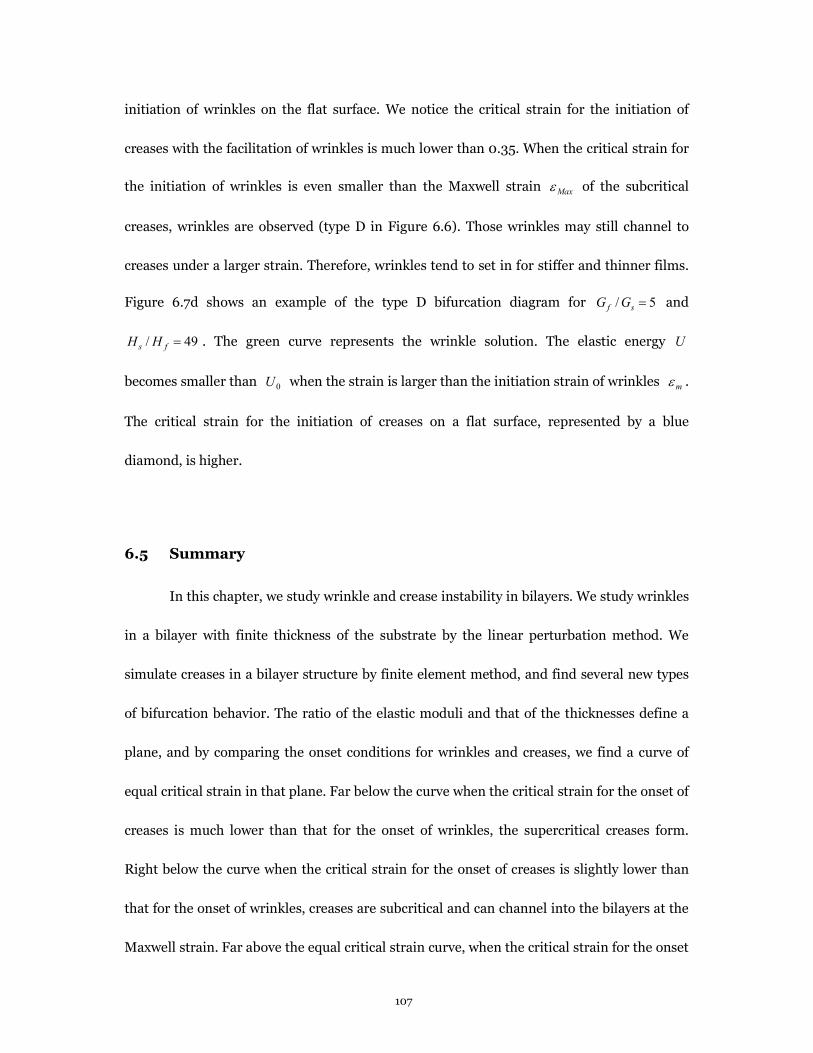
107

initiation of wrinkles on the flat surface. We notice the critical strain for the initiation of

creases with the facilitation of wrinkles is much lower than 0.35. When the critical strain for

the initiation of wrinkles is even smaller than the Maxwell strain Maxe of the subcritical

creases, wrinkles are observed (type D in Figure 6.6). Those wrinkles may still channel to

creases under a larger strain. Therefore, wrinkles tend to set in for stiffer and thinner films.

Figure 6.7d shows an example of the type D bifurcation diagram for 5/ =sf GG and

49/ =fs HH . The green curve represents the wrinkle solution. The elastic energy U

becomes smaller than 0U when the strain is larger than the initiation strain of wrinkles me .

The critical strain for the initiation of creases on a flat surface, represented by a blue

diamond, is higher.

6.5 Summary

In this chapter, we study wrinkle and crease instability in bilayers. We study wrinkles

in a bilayer with finite thickness of the substrate by the linear perturbation method. We

simulate creases in a bilayer structure by finite element method, and find several new types

of bifurcation behavior. The ratio of the elastic moduli and that of the thicknesses define a

plane, and by comparing the onset conditions for wrinkles and creases, we find a curve of

equal critical strain in that plane. Far below the curve when the critical strain for the onset of

creases is much lower than that for the onset of wrinkles, the supercritical creases form.

Right below the curve when the critical strain for the onset of creases is slightly lower than

that for the onset of wrinkles, creases are subcritical and can channel into the bilayers at the

Maxwell strain. Far above the equal critical strain curve, when the critical strain for the onset

108

of wrinkles is much lower than that for the onset of creases, wrinkles form. Right above the

curve, even when the critical strain for the onset of creases is higher than that for the onset of

wrinkles, subcritical creases can still channel at the Maxwell strain, which could be much

lower than the critical strain for the onset of creases in a homogeneous material, as long as

the Maxwell strain is lower than the critical strain for the initiation of wrinkles. When the

Maxwell strain is higher than the critical strain for the initiation of wrinkles, wrinkles form

first, but a further compression causes the strain at the troughs of the wrinkles to be high

enough to initiate creases, and wrinkles transit to creases subcritically.

109

Chapter 7

Role of substrate pre-stretch in post-wrinkling

bifurcations

7.1 Introduction

Wrinkles form when a thin stiff film supported on a soft substrate is compressed

beyond a critical strain. When the compression is slightly above the critical strain, the

wrinkles are periodic. The wavelength of the wrinkles is determined by a balance between

the deformation of the substrate, which favors short wavelengths, and the bending of the

film, which favors long wavelengths [10, 76]. By controlling the onset and evolution of

wrinkles in a number of different material systems, researchers have demonstrated a wide

range of applications. These include the fabrication of materials with changeable wetting

[34-37], adhesive [8, 31, 32], and optical properties [37, 40, 41], the measurement of

mechanical characteristics [14, 22-26] of thin films and soft substrates, and the use of

wrinkles as templates for self-assembly [27-29], in microfluidic [19-21], photovoltaic [16-18]

and flexible electronic devices [13-15, 218], and for alignment of cultured cells [29, 30, 219].

When compressed sufficiently far beyond the onset of wrinkling, however, new

deformation modes may appear, with characteristics that depend sensitively on the details of

the substrate response [147]. For a thin elastic film supported on a viscous substrate,

wrinkles lose their periodicity and transition to localized folds once the displacement applied

approaches one third of the initial wrinkling wavelength [74, 151]. The transition to localized

110

deformation may even lead to the fracture of the film [220]. For an elastomeric foundation,

wrinkles lose their initial periodicity through the emergence of sub-harmonic modes due to

nonlinear contributions to the elastic response of the substrate [82, 149]. Typically, a

progression from wrinkles to a period-doubled state is observed, followed by a

period-quadrupled state, and finally the formation of self-contacting folds [95, 145, 147]. The

emergence of sub-harmonic spatial modes in this context is analogous to appearance of

temporal sub-harmonics for a non-linear oscillator [145].

In light of the key role played by the substrate in driving post-wrinkling bifurcations,

it follows that this behavior should be highly sensitive to the state of the substrate, for

example the presence of a compressive or tensile pre-stress. In spite of this expectation,

however, only a limited number of studies along these lines have been conducted. In

particular, Hutchinson and co-workers have predicted the emergence of localized ridges as a

different type of post-wrinkling bifurcation for large substrate pre-tension from numerical

modeling [75, 155]. The application of in-plane pre-tension causes a softening of the outward

deflection of the substrate relative to the inward deflection and hence promotes the

formation of ridges. Conversely, the application of in plane pre-compression stiffens outward

deflection of the substrate relative to inward, favoring the formation of folds. While a few

experiments have indicated the emergence of ridges [155-157] or other modes of strain

localization [99] with pre-tension, the level of agreement with theory remains unclear.

Further, there has been little work focused on the case of substrate pre-compression. Thus,

there remains much to understand about how post-wrinkling behavior depends on substrate

pre-stretch.

111

The critical importance of a pre-stretched substrate is demonstrated by the simple

experimental result shown in Figure 7.1. Using an approach that will be described in detail

below, a soft elastomeric substrate is subjected to: (a) a tensile pre-stretch, (b) no pre-stretch,

or (c) a compressive pre-stretch, prior to formation of the stiff skin. At the same applied

nominal film strain, the resulting morphologies vary dramatically. With substrate

pre-tension, the surface remains uniformly wrinkled; with no pre-strain, it shows the clear

emergence of a sub-harmonic (period-doubled) mode; and with pre-compression, it shows a

highly irregular ‘chaotic’ pattern. The aim of the study in this chapter is to establish, through

a combination of experiments and simulations, how substrate pre-stretch alters the onset

and evolution of post-wrinkling modes as well as to understand the chaotic emergence of

different sub-harmonic modes by adopting a general method to study symmetry breaking

from a periodic structure.

Figure 7.1 Optical profilometry is used to characterize the surface profiles of films at similar nominal

strains εf on substrates with varying amounts of pre-stretch λ0. (a) At εf = 0.16 and λ0 = 1.3, uniform

wrinkles are observed. (b) At εf = 0.17 and λ0 = 1.0, period doubling has just begun to emerge. (c) At εf

= 0.15 and λ0 = 0.7, ‘chaotic’ post-wrinkling is found.

112

7.2 Methods

7.2.1 Experimental setup

Our experiments rely on an elastic trilayer system modified from a recently described

approach (Figure 7.2) [173]. A 400-mm-thick soft (shear modulus ms = 12.5 kPa)

poly(dimethylsiloxane) (PDMS) substrate is attached to a 1-mm-thick stiffer (m= 260 kPa)

PDMS mounting layer that has been uniaxially stretched to an initial length L0. This bilayer

is then partially released, or stretched further, to a new length L, placing the substrate under

a pre-stretch λ0 = L/L0. The importance of the mounting layer is that it allows for the

substrate to be loaded under pre-compression without undergoing macroscopic buckling.

Next, the surface is exposed to UV/ozone, which converts the top layer of the PDMS

substrate into a gradient-modulus silicate film with an effective film thickness of 3-8 mm that

shows excellent adhesion to the substrate [221]. We consider the film to be stress free at this

point, although we note the possibility for a slight residual stress due to mismatches in

thermal expansion and/or oxidation-induced changes in volume. A subsequent partial

release of the mounting layer to length l now places the bilayer under compression, which we

characterize in terms of the nominal strain applied to the film εf = (L-l)/L. The subsequent

wrinkling and post-wrinkling behavior of the surface as a function of applied strain is then

characterized by in situ optical profilometry. Using a defect in the wrinkling pattern as a

point of reference, we track the same region while increasing the compressive strain in the

film.

113

Figure 7.2 A schematic of the experimental procedure. An elastomeric substrate is attached to a

pre-stretched mounting layer, deformed to λo, and exposed to UV/O3 to form a stiff film layer. The stiff

film is compressed with strain εf by partially releasing the mounting layer.

7.2.2 Experimental details

A trilayer system was used to independently vary the compression applied to the

substrate and the silicate film. A silica reinforced vinyl-terminated polydimethylsiloxane

(PDMS) mounting layer (DMS-V31S15, Gelest Inc.) with a shear modulus 260 kPa and

thickness 1 mm was uniaxially pre-stretched on a stretcher. A pre-cured substrate with

thickness of approximately 400 mm composed of a PDMS elastomer (Sylgard 184, Dow

Corning) with a 50:1 weight ratio of base to crosslinker (shear modulus 12.5 kPa based on

dynamic mechanical analysis) was attached to the pre-stretched mounting layer using a thin

(2-5 mm thick) layer of uncured PDMS with the same composition as the substrate. This

bilayer assembly was placed in an oven at 60 ºC for 4 h to bond the layers, and then allowed

to cool to room temperature over 30 min before deforming the mounting layer to put the

substrate under a pre-stretch λ0. The substrate was left at λ0 for 30 min before being placed

114

in a UV/O3 cleaner for 25 min to convert the surface of the PDMS substrate into a stiffer

oxide layer. For each sample, we determined the amplitudes and spacings between at least

seven neighboring wrinkles from optical profilometry. The oxide films were found to have

effective thicknesses of 3-8 mm and shear moduli of 620 kPa – 3.8 MPa as determined by

fitting the dependence of the wrinkle amplitude and wavelength on film strain for samples

with no substrate pre-stretch via the classical buckling equations as described by Stafford

and co-workers [22, 23]. For any given sample, the respective uncertainties in these

quantities were less than 0.6 mm and 50 kPa; the large ranges determined for different

samples therefore presumably reflect slight differences in sample position within the UV/O3

cleaner. However, as the film modulus is larger than the substrate modulus by a factor of 50

– 300, this variation should not play a significant role in the observed behavior.

Compression was applied to the trilayer by relaxing the pre-stretch of the mounting layer.

Optical profilometry (Zygo NewView 7300) was used for in-situ characterization of

the height profiles of the sample surfaces using MetroPro 8.3.2 software. The 5x and 10x

lenses were utilized as well as the stitch application to characterize a large area of the sample.

At high film strains only the data points from the crest and trough could be imaged due to

the steep angles of the surface; a spline was used to fill in the missing segments of the surface

profiles in Figure 7.1 and Figure 7.6. Laser scanning confocal fluorescence microscopy (Zeiss

LSM 510 Meta) was used to characterize the shape of the wrinkles. Fluorescent labeling of

the substrate was accomplished by adding 4.5 mg of fluorescein-o-acrylate in 1,4-dioxane per

1 g of PDMS prior to curing. During imaging, a refractive index matching fluid consisting of

72% glycerol and 28% water (weight percent) was used along with a 25x variable immersion

115

lens. Several two-dimensional frames were taken and manually stitched together by aligning

peaks and troughs of the wrinkles to cover a larger area of the sample.

7.2.3 Finite element simulations

The commercial finite element software ABAQUS was used to computationally study

the effect of pre-stretch on post-wrinkling bifurcations. The substrate was uniaxially

pre-stretched and then the film-substrate bilayer compressed under plane strain. Both the

film and substrate were modeled as incompressible neo-Hookean materials, and the free

energy of neo-Hookean material with a pre-stretch was implemented by a user-defined

subroutine UMAT. For all the simulations except Figure 7.3, the modulus ratio of the film to

substrate was set to 50, and the thickness ratio of the bilayer to the film was chosen as 50,

both of which roughly match the experimental conditions. To break the symmetry of the

surface during compression, the first and second eigenmodes obtained by a linear

perturbation step were introduced as initial imperfections with very small amplitudes

(roughly 1/2000 times the film thickness).

We call the wrinkle wavelength lw. When we simulate the critical strain for period

doubling (Figures 7.3 and 7.5), the simulation sample length is chosen as lw. To understand

chaotic period multiplication (Figures 7.8-7.13), we calculate the energy of different periodic

states: wrinkling with the initial periodicity, period doubling, tripling and quadrupling. To

realize these different periodicities, we simulate samples with lengths lw/2, lw, 3lw/2 and 2lw

respectively. Symmetry condition is added on one boundary and uniform strain is applied on

the other boundary. Static method is used for all the simulations.

116

7.3 Results

7.3.1 Effect of substrate pre-stretch on period doubling

We plot measured amplitudes for several different levels of pre-strain (l0 = 0.7 – 1.2)

in Figure 7.3 (black triangles). The amplitude associated with a given feature on the surface

is defined as half of the average out-of-plane displacement between a given ‘trough’ and its

two neighboring ‘crests’. For each sample, at least seven features are measured. The critical

strain for wrinkling varied for different samples between 0.03-0.05, while the wrinkle

wavelength was lw = 100 – 160 mm. This degree of variability is apparently due to slight

differences in the position of the sample relative to the UV light source during oxidation.

Using the approach of Stafford and co-workers [22], the effective thicknesses of the silicate

layers are estimated for each sample with no substrate pre-stretch as hf = 3 – 8 mm, with

shear moduli of mf = 620 kPa – 3.8 MPa, corresponding to modulus mismatch values (mf/ms)

of 50 – 300. These large ranges in effective film thickness and modulus are the result of

variations between different samples. However, as shown by Cao and Hutchinson, the

modulus mismatch does not affect the critical strain for post-wrinkling bifurcations if the

mismatch is above 10 [75].

In the wrinkle regime, the amplitudes are nearly homogeneous, as can be seen from

the small amount of scatter in Figure 7.3 (standard deviations in wrinkle amplitudes are

typically less than 1 mm), and grow with increasing strain. However, at a sufficiently large

value of εf, a post-wrinkling bifurcation is observed in which some wrinkles grow in

amplitude while their neighbors shrink. As seen in Figure 7.3a-c, pre-stretches from l0 =

1.0 – 1.2 show a clean bifurcation corresponding to a period doubled state, as shown by Brau

117

et al. for the case of l0 = 1 [145]. We denote the strain at which this first post-wrinkling

bifurcation is observed as εpw, identified in practice as the point at which the standard

deviation of wrinkle amplitudes show a dramatic increase. For the case of l0 = 1, we verified

that the period doubling bifurcation showed no apparent hysteresis from initial loading, to

unloading, and subsequent reloading (Figure 7.4), suggesting that plastic deformation plays

little if any role in this process.

Figure 7.3 Bifurcation curves of the wrinkle amplitude as a function of film strain for substrates

pre-stretched to l0 = (a) 1.2, (b) 1.1, (c) 1.0, (d) 0.9, (e) 0.8 and (f) 0.7. The experimental data (black

triangles) reveal a gradual shift of the bifurcation point as well as an increase in distribution of

amplitudes past epw with a decrease in l0. Simulations (red lines) show good agreement with the

experimental data.

For λ0 = 1 (Figure 7.3c), we measure a value of εpw = 0.18, which is in good agreement

with the values reported by Brau et al. of 0.17 - 0.20 for a true bilayer system [145]. When the

substrate is under slight pre-tension, the period-doubled bifurcation shifts to higher strains

but remains otherwise qualitatively similar; at λ0 = 1.2 we measure εpw = 0.23 for the sample

characterized in Figure 7.3a and at λ0 = 1.1 we measure εpw = 0.22 for the sample in Figure

7.3b. Under slight pre-compression the bifurcation occurs at lower film strain; at λ0 = 0.9

118

and λ0 = 0.8 (Figure 7.3d-e), we find εpw = 0.11 and εpw = 0.10, respectively. While a clear

bifurcation into a bimodal collection of larger and smaller amplitudes can still be seen in this

case, consistent with period doubling, the spread in amplitudes for each population is larger

than for λ0 = 1 and λ0 = 1.2.

Figure 7.4 (a) Bifurcation curves for l0 = 1.0 show no detectable hysteresis from the first loading

cycle to unloading and subsequent reloading. Optical profilometry images of the surface (b) during the

first loading at a film strain of 0.24, and (c) during the second loading at a film strain of 0.23.

This non-uniformity becomes dramatically more pronounced for a film on a substrate

with a larger pre-compression, λ0 = 0.7 (Figure 7.3f). In this case, a clean bifurcation is lost,

replaced instead by the emergence of a broad spread of amplitudes at a strain of εpw = 0.06,

which is only slightly above the critical strain for wrinkling, εw = 0.04. The transition from

regular wrinkles to irregular, or ‘chaotic’, structures occur over such a small range of strain

that when plotted on the same scale as the other samples in Figure 7.3a-e, the distinction

between wrinkling and post-wrinkling is completely obscured; however, the inset to Figure

7.3f shows that indeed a narrow range of regular wrinkling can be discerned.

To better understand these effects, we model the system using the commercial finite

element software ABAQUS. Both the film and substrate are taken to be incompressible

119

neo-Hookean materials. For a ratio of the film to substrate modulus of only 50 – 300, as

studied here, the maximum strain in the film can be as large as ~ 0.20 in our simulations.

Thus, it is necessary to use a non-linear hyperelastic model for both the film and substrate.

However, as the range of strains is still modest, the neo-Hookean model should provide a

reasonable description of both materials. The substrate is uniaxially pre-stretched while the

film/substrate bilayer is subsequently compressed under plane strain, which is similar to the

condition in the experiments. To simulate the period doubled state, we choose a unit cell of

width lw, the wrinkle wavelength. Symmetry is maintained across one boundary and uniform

strain is applied on the other boundary. A small amplitude initial imperfection is introduced

to break the translational symmetry of the surface. More details about the simulations of the

period doubled state will be discussed below. When compressive strain is incrementally

applied, the surface initially remains flat and then forms wrinkles after a critical strain. With

further increase in strain, the wrinkle amplitude grows but the nominal wavelength does not

change. After a second critical strain, wrinkles lose their original periodicity through a

supercritical period-doubling bifurcation. We record the second critical strain as εpw.

In Figure 7.3, we plot the simulation results for wrinkle amplitudes with different

substrate pre-stretches as red lines. From the experimentally measured wrinkle wavelength,

and the dependence of wrinkle amplitude on strain, we estimate the film thickness by fitting

the classical buckling equations [22], as before. For the effective film modulus, however, we

make use of the theoretical prediction that takes into account substrate pre-stretch and

assumes infinite substrate thickness [75]. The modulus ratios of the film to substrate

estimated in this fashion are (a) 120, (b) 200, (c) 50, (d) 130, (e) 225 and (f) 35, while the

120

film thickness are (a) 5.8 mm, (b) 6.0 mm, (c) 8.0 mm, (d) 6.6 mm, (e) 5.5 mm and (f) 7.8 mm.

In the simulations, we choose a modulus ratio to match the experimental value for each plot.

The ratio of the total thickness to the film thickness is fixed at a representative value 50 in all

cases, since the ratio has no effect on the wrinkling and post-wrinkling as long as the

substrate is much thicker than the film, and can be treated as infinite. As seen in Figure 7.3,

the simulations generally agree well with the experimental results, in terms of both the

location of the post-wrinkling bifurcation and the subsequent evolution of amplitudes. The

agreement of the cases with pre-tension in the substrate is slightly better than with

pre-compression. A possible reason is the competition between different post-wrinkling

bifurcation modes, which clearly influences the behavior at large pre-compression, as we

discuss further below.

Figure 7.5 shows the dependence of εpw on λ0, obtained from finite element

simulations and experiments on at least 3 different samples at each λ 0. In this simulation

and the remainder of the chapter, the ratio of the film modulus to substrate modulus is fixed

as 50, since εpw is almost independent of the modulus ratio as long as the modulus ratio is

larger than 10 [75]. The ratio of the total thickness to the film thickness is also fixed as 50,

which is large enough for the thickness of the substrate to be considered as infinite. When

there is no pre-stretch in the substrate, εpw is calculated to be around 0.18, which matches

the experimental value of 0.18 ± 0.02. A monotonic increase in εpw with λ0 is seen:

pre-compression in the substrate decreases εpw, while pre-tension increases εpw. Under

pre-tension, e.g. λ0 = 1.2, the finite element result of εpw = 0.26 agrees well with that from

experiments (0.27 ± 0.07). Under pre-compression, e.g. at λ0 = 0.7, the respective

121

experimental and simulation results of εpw = 0.05 ± 0.02 and 0.06 are again in agreement.

Overall, the simulations in Figures 7.3 and 7.5 show almost quantitative agreement with

experimental data, and the qualitative trend of εpw monotonically and strongly increasing

with λ0 over this range of substrate pre-stretch is clear in both cases.

Figure 7.5 The critical film strain for post-wrinkling bifurcation epw is plotted against the substrate

pre-stretch l0. The solid line represents finite element results and the solid symbols represent

experimental results, with the error bars corresponding to minimum/maximum values for at least 3

samples. As pre-stretch increases, the film strain required for post-wrinkling bifurcation increases.

7.3.2 Chaotic period multiplication under large substrate pre-compression

We next consider the irregularity of amplitudes observed during post-wrinkling

bifurcation for substrates under pre-compression. In Figure 7.6, we compare in detail the

evolution of surface topography with increasing film strain for samples with λ0 = 1.0 and 0.7.

Color maps of the surface profiles are shown over large areas of the sample (Figure 7.6a-c,

e-g), along with line profiles (Figure 7.6d, h) at the locations indicated. The profiles are taken

at nearly the same position on each sample, and plotted with an x-axis normalized by (1- ef)

to vertically align each crest and trough so that its evolution with film strain can be easily

observed.

122

Figure 7.6 The surface profile of a sample with pre-stretch 1.0 at film strains of (a) 0.083, (b) 0.16, (c)

0.23. (d) One-dimensional profiles at the locations indicated by the solid lines in (a-c). The surface

profile of a sample with pre-stretch 0.7 at film strains of (e) 0.045, (f) 0.063 and (g) 0.11. (h)

One-dimensional profiles at the locations indicated by the solid lines in (e-g).

With no pre-stretch, the sample evolves from the wrinkled state (green trace in

Figure 7.6d) at ef = 0.083 to a period-doubled state at ef = 0.16 (blue trace) and a

period-quadrupled state at ef = 0.23 (red trace). The amplitudes evolve in a fairly regular

fashion across the entire sample, except in regions close to a defect in the wrinkling pattern

(i.e., as seen to the lower left of Figures 7.6a-c and correspondingly to the left side of the

traces in Figure 7.6d).

With a pre-compression of λ0 = 0.7, however, dramatically different behavior is

observed. A regular wrinkle pattern is first observed, as seen for ef = 0.045 (Figure 7.6e,

green trace in Figure 7.6h), but rapidly evolves into a set of deep features with irregular

spacing by ef = 0.11 (Figure 7.6g, red trace in Figure 7.6h). Examination of the behavior at

intermediate strains, e.g. at ef = 0.063 suggests that this pattern emerges through the

competition between multiple different sub-harmonic modes with periodicities of 2, 3, and 4

times the fundamental wrinkle mode. In other words, some regions show behavior locally

123

characteristic of period doubling (two troughs that grow in depth separated by one that

becomes more shallow), while others show characteristics of period tripling (deep troughs

separated by two shallow troughs) and quadrupling (separation by three shallow troughs).

Figure 7.7 Laser scanning confocal fluorescence cross-sections of compressed bilayers with substrate

pre-compression of l0 = (a) 1.0, (b) 0.9, and (c) 0.7, showing the emergence of post-wrinkling modes

with increasing nominal film compression ef.

Similar behavior can be observed by using laser scanning confocal fluorescence

microscopy to characterize samples with fluorescently labeled substrates. With no substrate

pre-stretch (Figure 7.7a), regular wrinkles first develop at ef = 0.04, then grow in amplitude

before period doubling takes place at ef = 0.17. When the substrate is under a small amount

of pre-compression, λ0 = 0.9 (Figure 7.7b), wrinkles first give way to a shallow period

doubled state at ef = 0.14, and by ef = 0.17, the sample is well past the onset of period

doubling, with the amplitude of the diminishing wrinkles approaching zero. By ef = 0.22, the

bilayer with λ0 = 0.9 has already transitioned to the period quadrupled state; whereas for λ0

124

= 1.0, the sample remains in the period doubled state even at a slightly higher film strain of

0.24. With larger pre-compression, λ0 = 0.7 (Figure 7.7c), wrinkles form but are soon

followed by a ‘chaotic’ surface pattern with shallow regions of the period doubled, period

tripled and period quadrupled states. Interestingly, this behavior shows variability across the

transverse direction of the sample, as seen in Figure 7.6g. We suspect this behavior arises

because different regions of the sample spontaneously break the symmetry of the wrinkle

pattern in different ways, leading to the presence of ‘domain boundaries’ where one set of

deep features meets another, mismatched set. However, further study is required to better

understand this process.

Figure 7.8 Various post-wrinkling bifurcations obtained by finite element simulation. (a) Wrinkles

maintaining the initial periodicity. (b) Period doubling. (c) Low-energy tripling. (d) High-energy

tripling. (e) Period quadrupling. The film strain is εf =0.11 and the substrate pre-stretch is l0 =0.7.

The emergence of such chaotic behavior can be anticipated based on the analogy to

the nonlinear oscillator [145, 222-224], which is well-known to show chaotic behaviors in

certain regimes. However, to provide a better understanding of the driving force in the

current system, we use finite element methods to compare the energies of the different

sub-harmonic modes. To enable such comparisons at equivalent levels of compression, we

employ simulation cells with several different sizes, boundary conditions, and initial

125

imperfections, to enforce different symmetries on the post-wrinkled states. For example,

Figure 7.8 shows simulated surface height profiles for different modes at a constant film

strain of εf = 0.11 and pre-stretch of l0 = 0.7: wrinkling that maintains the initial periodicity

(Figure 7.8a), period doubling (Figure 7.8b), low-energy tripling (Figure 7.8c), high-energy

tripling (Figure 7.8d) and period quadrupling (Figure 7.8e).

To enforce the initial wrinkle period to be conserved throughout the application of

the strain, as in Figure 7.8a, we simulate a unit cell with half the nominal wrinkle wavelength

lw/2. One boundary of the unit cell is chosen at a trough of the wrinkles and the other is

chosen at the neighboring peak. We apply reflection symmetry on one boundary and uniform

strain on the other boundary, so that both boundaries are kept flat. The corresponding

energy per wavelength lw is calculated and called U1.

To study the bifurcation from a periodic wrinkled state to a period-doubled state

(Figure 7.8b), we use a unit cell of width lw. We can position the boundaries of the unit cell in

two ways: at the troughs of two neighboring wrinkles (Figure 7.9b), or at the peaks (Figure

7.9c). The simulations start with a nearly flat surface with small amplitude (1/2000 times the

film thickness) prescribed imperfections, shown in Figure 7.9b and c greatly magnified in

amplitude for visual clarity. In both cases, symmetry condition is applied on one boundary

and uniform strain is applied on the other boundary. Our simulations indicate that the first

choice of boundaries (Figure 7.9b) leads to period-doubling at the critical strain εpw, and we

call the energy per wavelength lw of this configuration U2. By contrast, for the second choice

of boundaries, the system retains the initial wrinkle periodicity and does not undergo period

doubling.

126

Figure 7.9 Simulating bifurcation from a periodic wrinkled state to a period-doubled state. (a) The

wrinkled state with period lw. The finite element simulations use unit cells of width lw of two types.

(b) A unit cell with boundaries at the troughs of neighboring wrinkles bifurcates into the

period-doubled state at a critical strain εpw. (c) The other type of unit cell with boundaries at the peaks

of neighboring wrinkles remains in the periodic wrinkled state and does not bifurcate. The

simulations start with a nearly flat surface with prescribed imperfections shown in (b) and (c). For

visual clarity, the amplitude of the imperfections has been greatly magnified.

To study the bifurcation to a period-tripled state (Figure 7.8c and d), we use a unit cell

of width 3lw/2, which allows for period-tripling but prevents period-doubling. There is only one

choice for placing the boundaries of the unit cell, with one boundary at a trough and the other

boundary at a peak of the wrinkles (Figure 7.10a). Again, we apply symmetry condition and

uniform strain to the two boundaries. The period-tripled state can lead to two modes (Figure

7.8c and d), which are selected through the initially prescribed small amplitude imperfections,

as shown in Figure 7.10b and c. In one mode of period tripling, of the three neighboring

troughs, one becomes deeper and the other two become shallower (Figure 7.8c and 7.10b). In

the other mode of period tripling, of the neighboring troughs, one becomes shallower and the

other two become deeper (Figure 7.8d and 7.10c). We call the energy per wavelength lw of both

modes U3 . Figure 7.10d plots the difference in the energies between the two tripling modes and

the doubling mode, U3-U2, as a function of the film strain for a pre-stretch of l0 =0.7. We

127

normalize the energies by mslwhf, where hf is the thickness of the film. The mode in Figure

7.10b has a lower energy than the mode in Figure 7.10c, and thus for the remainder of the

chapter, we only consider the former, lower energy, mode of period tripling. Remarkably, this

low-energy tripling mode has a lower energy than the period-doubling mode at sufficiently

large film strains—a point to which we will return below.

Figure 7.10 Simulating bifurcation from a periodic wrinkled state to a period-tripled state. (a) The

wrinkled state with period lw. The finite element simulation uses a unit cell of width 3lw/2, with one

boundary at a trough and the other boundary at a peak. This unit cell leads to two modes of period

tripling. (b) In one mode, of the three neighboring troughs, one becomes deeper and the other two

become shallower. (c) In the other mode, one becomes shallower and the other two become deeper.

The simulations start with a nearly flat surface with prescribed imperfections shown in (b) and (c),

where the amplitude has been greatly magnified. (d) The difference in the energies of the tripling and

doubling modes, U3-U2, as a function of the film strain. The pre-stretch is l0 =0.7. The mode in (b) has

a lower energy than the mode in (c). Furthermore, the mode in (b) has a lower energy than the

period-doubled state beyond a critical film strain, but the mode in (c) always has a higher energy than

the period-doubled state.

128

To study the bifurcation to a period quadrupled state (Figure 7.8e), we use a unit cell of

width 2lw, which allows both period doubling and quadrupling. Similar to period doubling, we

can choose the boundaries of the unit cell in two ways: at two troughs (Figure 7.11b) or at two

peaks (Figure 7.11c). Moreover, similar to period tripling, there can be more than one mode of

the period-quadrupled states even when the boundary of the unit cell is chosen. Here, we will

not go into details regarding these different modes, but instead focus on the mode of

quadrupling corresponding to that observed in experiments (Figure 7.8e), which is selected by

the prescribed imperfections shown in Figure 7.11b. In this case the system first undergoes

period doubling, followed by period quadrupling, and we denote the energy per wavelength lw

as U4.

Figure 7.11 Simulating bifurcation from a periodic wrinkled state to a period-quadrupled state. (a)

The wrinkled state with period lw. (b) The finite element simulation uses a unit cell of width 2lw, with

boundaries at two troughs of the wrinkles. With the initial prescribed imperfections shown in (b),

magnified in amplitude for clarity, the system undergoes period quadrupling at a critical strain after

period doubling. (c) If the boundaries are chosen at the peaks of the wrinkles, period quadrupling

cannot happen.

129

Figure 7.12 The normalized energy of the period-doubled state U2, tripled state U3, and quadrupled

state U4 relative to the energy of the periodic wrinkled state U1. The pre-stretch in the substrate is (a)

λ0 = 1.0, (b) λ0 = 1.2, (c) λ0 = 0.85 and (d) λ0 = 0.7. The inset in (d) shows a magnification of the region

of ef = 0.06 - 0.13.

In Figure 7.12a-d, we plot the normalized energy by which each of the configurations

U2, U3, U4 differ from the wrinkled state U1, as a function of the applied strain ef. When a

given curve falls below 0, the corresponding type of period multiplication is energetically

favorable, with the lowest energy curve representing the ground state. As seen in Figure

7.12a for no pre-stretch, the system remains in the wrinkled state and thus all of the curves

stay at an energy of 0, until a strain of ef = 0.19. Beyond this point, the curves for U2 and U4

become negative, corresponding to the period-doubled state. At a strain of ef = 0.25, the

130

curve for U4 becomes lower in energy than U2, corresponding to the period-quadrupled state.

Over this range of strain, the energy U3 remains above both U2 and U4, and thus period

tripling is energetically disfavored. These findings are in excellent agreement with our

experiments at λ0 = 1.0, as well as previous work, showing clean period doubling and period

quadrupling bifurcations [95, 145, 147].

The pre-tensioned substrate stabilizes both the wrinkled and period-doubled states,

as seen in Figure 7.12b for λ0 = 1.2. Here, the onset of period doubling is delayed until ef =

0.25, while over the range of strain studied (up to ef = 0.32) period quadrupling is not

observed at all, and U3 remains well above U2. The simulation results show excellent

agreement with our experimental findings that period doubling is shifted to higher strains

when there is pre-tension in the substrate and no period quadrupling is observed over the

range of ef studied.

In contrast, the pre-compressed substrate de-stabilizes both the wrinkled and

period-doubled states compared to the period-tripled and quadrupled states (Figure 7.12c

and d). As seen in Figure 7.12c for λ0= 0.85, the curve for U2 falls below zero at a strain of

0.13, only slightly before U3 does, at 0.15. The period-tripled state U3 then falls below U2 and

U4 at a strain of 0.18. As seen in Figure 7.12d for λ0= 0.7, the curves for U2 and U3 fall below

zero at very similar strains (ef = 0.07 – 0.08). The period-quadrupled state U4 falls below U2

at only slightly higher strain (ef = 0.10), and remains very close to U3 for larger strains.

Because period doubling, tripling and quadrupling all happen at strains close to the

formation of wrinkles, wrinkles are still very shallow, and the energies of each of these

subharmonic modes in the range of ef = 0.07 – 0.10 are very close to each other. The inset of

131

Figure 7.12d magnifies the energies in this region of strain.

We further illustrate the effect of pre-stretch by plotting the difference between U3

and U2 for several values of λ0 (Figure 7.13). The pre-compressed substrate greatly reduces

the energy difference between the period-tripled state and the period-doubled state.

Presumably, this similarity in energy means that the presence of defects or even slight spatial

variations in material properties would lead to local biases in favor of a given sub-harmonic

mode, thus yielding a globally chaotic behavior. The prediction from the simulation is

qualitatively in very good agreement with our experimental observations.

Figure 7.13 The difference in energy between the period-tripled state U3 and the period-doubled

state U2 for different values of the substrate pre-stretch λ0.

7.4 Summary

Our study reveals the strong effect of substrate pre-stretch on post-wrinkling

bifurcations. Pre-stretch shifts the critical strain for period doubling: modest amounts of

pre-tension are found to stabilize wrinkles to higher strains, while modest pre-compression

promotes the emergence of sub-harmonic modes at lower strains. For large substrate

132

pre-compression, a new type of spatially chaotic behavior is found. A newly developed

computational approach allows for the study of symmetry breaking from a periodic structure

by the emergence of different sub-harmonic modes through the prescription of different

simulation cell sizes, initial imperfections, and boundary conditions. The computational

results reveal that energies of the different subharmonic modes become similar when the

substrate is pre-compressed, thus eliminating the preference for a clean sequence of period

doubling and quadrupling bifurcations. We anticipate that substrate pre-stretch will be an

important parameter in future efforts to control the morphologies of wrinkled and

post-wrinkled surfaces.

133

Chapter 8

Ridge localizations and networks under equi-biaxial

loading

8.1 Introduction

The intriguing buckling patterns exhibited by bilayer systems composed of a thin stiff

film bonded to a thick elastomeric substrate have been studied extensively in recent years

both experimentally and theoretically. Under compression, the film is constrained by the

substrate and buckles with a wavelength that is usually large compared to the film thickness

yet small compared to substrate thickness. The most common patterns observed are the

sinusoidal wrinkle mode when compression in one direction is dominant [22], and the

herringbone mode [82, 86] and the labyrinth mode [81, 82, 86] under states of equi-biaxial

compression.

This chapter is part of the ongoing research effort in the soft materials community to

produce and manipulate specific buckling patterns [99, 156]. Most of the previous work has

focused on buckling patters of bilayer systems under small compression. Recent work,

however, has demonstrated that large compression of a bilayer system can engender other

surface patterns such as period-doubling [145] and folding [74, 146], opening the way for the

creation of a wider array of surface patterns. These post-wrinkling modes involve the large

strain behavior of the substrate and geometrical nonlinearity of the films in an essential way.

The focus of this chapter is on the post-wrinkling modes discovered most recently,

134

the ridge localization mode. While folds and creases protrude into the substrate, the ridge is

a large amplitude localization that pushes out from the substrate. This mode should be

characterized as localization because the large amplitude of the ridge is fed by flattening the

nearby wrinkle undulations resulting in ridges that are separated from each other by

expanses of relatively flat film. Thus, a distinct feature of the transition from wrinkles to

ridges is the abrupt increase of spacing from crest to crest. The ridge localization was

predicted to occur [75], and has been observed experimentally [99, 148, 155, 156], only when

a relatively large pre-stretch is imposed on the elastomeric substrate prior to film attachment.

Controlled incremental release of the pre-stretch of the thick substrate then imposes

compression on the film which drives buckling. The large substrate pre-stretch favors the

formation of the ridge mode [75]. The buckling pattern reported in this chapter consists of

localized ridge lines separated by relatively flat patches of film. Exploitation of high

pre-stretch produces these new high aspect convex structures which have potential for

expanding the range of surface morphologies for applications such as smart adhesion [32],

hydrophobic surfaces [15, 34, 35], and templates for micro-patterning [225].

This chapter features a method for applying equi-biaxial pre-stretch and release and

thereby complements recent related work on ridge formation which has primarily been

limited to uniaxial or plane strain pre-stretch [75, 99, 148, 155]. The present chapter also

highlights the underlying characteristics and nature of ridges, including emergence and

evolution aspects, which are still unclear due to the highly non-linear behavior of the system

caused by high pre-stretch. For the system and approach employed here delamination [99,

226, 227] and cracking [90] of the thin film, which often accompany wrinkling instabilities,

135

have been avoided.

The transition to the ridge buckling morphology is studied in a bilayer system

comprised of a thin stiff film attached to a relatively thick compliant substrate. The substrate

is subject to a large equi-biaxial pre-stretch prior to film attachment and then the bilayer is

incrementally unloaded producing equi-biaxial compression in the film. The experiments are

carried out using a specially designed micro-fluidic loading system. The system enables

equi-biaxial pre-stretch and incremental compression simply by changing pressure inside

the micro-fluidic chamber as used in [228], while more conventional loading systems [86,

156] require well-synchronized control of mechanical stretchers. Because mechanical

stretchers are not employed, our method can simultaneously handle several systems at the

scale of 1cm within the film deposition cavity, whose space is often limited. Using this system,

we clearly captured transitions from wrinkles to localized ridges and formation of a ridge

network surrounding flattened regions. In particular, the experiments reveal the evolution of

the ridge structure which involves propagation of individual ridges to form a network. The

influence on the geometry of the ridge is explored by varying the pre-stretch and the

thickness of the thin film. Further, finite element simulations have been carried out to obtain

conditions for localized ridge formation and propagation. Unlike sinusoidal or herringbone

wrinkles, the ridge is a finite amplitude mode, and the wrinkle to ridge transition is

subcritical as described more fully in conjunction with the simulations. As the pre-stretch is

released, once a ridge forms, it grows and saturates to a height comparable to its width.

8.2 Experimental results

136

Figure 8.1a illustrates the method of preparing the highly pre-stretched substrate. A

chamber capped by a flat layer of the elastomeric substrate material, Polydimethylesiloxane

(PDMS), is formed. The substrate layer is then stretched by filling the chamber with oil. With

the pressure inside the chamber held constant, an organic polymer material, Parylene-C, is

deposited on the surface to form the film. Prior to deformation the PDMS substrate layer has

a thickness in the range, 50=sh mm to 300 mm and a shear modulus, 33.0~sm MPa. The

Parylene film (thickness fh from 85 nm to 1.3 mm thick, shear modulus 58.0~fm GPa) is

stress-free as deposited. The stress-strain curves of PDMS and Parylene are given in

Appendix Figure C.1, and the detail of the fabrication is available in Appendix C.1. The

equi-biaxial pre-stretch 0l attained in the central region of the substrate is defined as the

ratio of the length after stretch L to the original length 0L , 00 / LL=l . An equi-biaxial

compressive strain, e , is exerted on the film in the central region when oil is released

incrementally from the chamber. The compressive strain is defined as Ll /1-=e where the

current length is l .

Compared methods such as thermal expansion [81] and swelling [82, 83, 229, 230]

for inducing equi-biaxial strain, the present method can induce pre-stretch greater than 1.5

and the magnitude of the pre-stretch can be readily adjusted by controlling the pressure

inside the chamber. The thickness of the substrate is selected to be at least 50 times that of

the film, and the film is about 2000 times stiffer than the substrate. The radius of the

chamber is 2 mm, and the effect on the instability due to the curvature of the chamber is

considered to be negligible (discussed in Appendix C.1).

137

Figures 8.1 (a) Schematic illustration showing the preparation of the highly pre-stretched bilayer

system using micro-fluidics. (b) Image of the experimental setup: Compressive strain is applied by

reducing the oil inside the chamber and a ridge structure emerges on the surface. (c) SEM image of

the ridge structure: the localized convex structure is observed concomitantly with a flattening of the

neighboring film surface.

Figures 8.1b and c show the typical morphology of the surface with ridges. Figure

8.1b shows an overview of an experimental setup taken by a microscope at point in the

release process where ridges have formed with the chamber still substantially inflated.

Figure 8.1c shows an image of Scanning Electron Microscopy of a surface of another sample.

This figure reveals localized ridges separated by extensive unbuckled regions. Unlike a

typical wrinkle or herringbone buckling pattern [82, 86] which fills the entire surface of the

film, a ridge is localized with extensive regions on both sides of the ridge being almost flat.

Furthermore, unlike creases and folds [74, 146] which protrude into the substrate, ridges

push upward from the substrate. These and other aspects of the ridge mode will be discussed

138

in further detail later in the chapter.

The scale of the ridges depends on the film thickness fh . In Figure 8.1b, with

1~fh mm, the width of the ridges is ~50 mm, while in Figure 8.1c, with fh ~100 nm, the

width of the ridges is ~5 mm. In neither of these cases has the Parylene thin film delaminated

from the PDMS substrate (a cross-sectional view is available in Appendix Figure C.2). The

pre-stretch and compressive strain in the central region are estimated by measuring the

height of the chamber at each stage of inflation or deflation, and the non-uniformity of the

pre-stretch of the system is considered to be negligible; see Appendix Figure C.3 for more

details.

An overview description of one experiment is now presented. As the equi-biaxial

compression in the film is increased by slowly releasing oil from chamber, wrinkles first form

and then, with further compression, wrinkles give way to ridges as seen in Figure 8.2. In this

experiment, 100=fh nm, 50=sh mm and the substrate has been pre-stretched to

59.10 =l . For this system, dimpled wrinkles, reflecting the equi-biaxial compressive stress

experienced by the film, cover the surface at 0.05e (Figures 8.2a and b). As the

compressive strain experienced by the film is further increased the dimples become more

like wrinkles (Figures 8.2c) and then, by 066.0=e , the transition to ridge-like features is

evident (Figures 8.2d and e). At 066.0=e , ridges are observed to advance flattening

neighboring regions under conditions when no oil is released from the chamber such that the

overall compression in the system is nominally fixed (Figure 8.2f). As will be shown later, the

critical compressive strain for ridge formation is only slightly above that for the wrinkle

pattern, and in the present study it has not been possible to experimentally resolve the

139

difference between the two critical strains.

Figure 8.2 Wrinkle to ridge transition. (a) In its initial state the surface of the chamber is flat. (b)

With compressive strain, the dimpled wrinkle pattern is engendered on the surface. (c) With increase

of the compressive strain, the dimpled wrinkle pattern transforms into the wrinkle pattern. (d) With

further compression, some peaks of the wrinkles increase their height and ridges are nucleated. (e, f)

Under essentially the same applied compression, ridges can propagate and flatten neighboring

surfaces.

Further experimental details on the development and evolution of a ridge network

are presented in Figure 8.3. For this experiment, the substrate is pre-stretched to a larger

value, 85.10 =l , enhancing ridge formation and the ensuing ridge network. In this case,

85=fh nm and 50=sh mm. As shown in Figure 8.3a, unconnected ridges are first formed

with wrinkles appearing perpendicular to the ridges. With the increase of compression, new

ridges nucleate and propagate perpendicularly to existing ones until they become blocked by

a pre-existing ridge (Figure 8.3b and c). A network of ridges is created; the few wrinkles still

present illustrate clearly the distinction between wrinkles and ridges. With the further

increase of compression, the network grows denser (Figure 8.3d and e) until there is no

space for new ridges to be nucleated and the network saturates (Figure 8.3f). The evolution

seen here for the ridge pattern is similar to the evolution of folds in a compressive bilayer

140

without pre-stretch reported in [146].

Figure 8.3 The formation of the ridge network: (a) In compression, unconnected ridges first appear.

(b-c) With the further increase of the compression, new ridges nucleate perpendicular to the existing

ridges. As marked with the dashed circles, wrinkled regions emerge before ridge nucleation and

become flattened after the formation of the ridge. (d-e) With even further increase of the compression,

the network grows denser, and (f) finally is completely packed. (g) Phase diagram of wrinkle/ridge

mode. Ridge structure appears with the pre-stretch 410 .>l . (h) Relationship between stiff film

thickness and width of the ridge. Fitting curve is fhw 34= . Relationship between height/width ratio

wA / of a ridge and stiff film thickness fh is embedded.

The dependence of the geometry of the ridge and the threshold pre-stretch lc

required for the formation of a ridge has been measured by systems with seven different

141

thicknesses of the Parylene film ranging from 85=fh nm (with 50=sh mm) to

3.1=fh mm (with 300=sh mm). For a given pre-stretch, 0l , the compressive strain e is

increased by release of the pre-stretch and the surface of the bilayer is carefully examined to

see the buckling patterns that emerge and, in particular, whether ridges form. The phase

diagram of wrinkle/ridge is plotted in Figure 8.3g. The threshold pre-stretch is

approximately 4.1=cl for ridge formation—that is, for smaller pre-stretches ridges are not

observed and for larger pre-stretches they are observed. The threshold appears to be

independent of the thickness of the stiff film, consistent with what is expected on

dimensional grounds for thick substrates. For cases in which ridges are formed, the width w

and the height A of the ridges (as defined in the inset of Figure 8.3h) are also measured

and plotted in Figure 8.3h. The measurements presented in the Figure 8.3h have been taken

for cases in Figure 8.3g in which the pre-stretch 0l is between 1.4 and 1.6. The width w is

proportional to the film thickness fh , and for the stiffness ratio of the present

film/substrate system the experimental results are fitted by 34 fw h= . If one imagines a

ridge to be the localization of a single wrinkle, one would expect the ridge width w to be the

same order as the wavelength of the wrinkle wl . In [75], the wavelength of a wrinkled linear

elastic film on a neo-Hookean substrate subject to an equi-biaxial pre-stretch 0l is

( )( ) 31300 1322

/)( lmlm += sffw hl . With 1750/ =sf mm and 5.10 =l , one finds fw hl 46= ,

which is on the same order as the experimentally measured wavelength in Figure 8.3h. In all

of these cases, the ratio of the ridge height A to its width w , wA / (inset of Figure 8.3h)

is significantly larger than the amplitude/wavelength ratio of the conventional wrinkle at

these compressive strains, i.e., ~ 0.1.

142

8.3 Finite element simulations

Numerical simulations employing the commercial finite element software, ABAQUS,

have been carried out to study and quantify the conditions for ridge formation. These

simulations go well beyond the initial plane strain studies [75], where ridges were first

discovered theoretically. In addition to systematically exploring the effect of equi-biaxial

pre-stretch on ridge formation, we have investigated the mechanics by which the ridges

propagate. Simulation details can be found in Appendix C.1, and details on the mechanics of

ridge formation and propagation can be found in Chapter 9.

To break the translational symmetry of the flat surface and initiate wrinkles, a very

small initial imperfection in the form of a slight surface waviness is introduced. The

formation of wrinkles and ridges is simulated under a generalized plane strain condition in

the 1-2 plane (as defined in Figure 8.4a) with an equi-biaxial pre-stretch 0l in the substrate

and the subsequent equi-biaxial compressive strain e applied to both film and substrate. In

keeping with generalized plane strain, the overall strains in the 1-3 directions are equi-biaxial,

but the displacements caused by the wrinkles or by ridges relative to the equi-biaxial flat

state are subject to the constraint of plane strain. The plane strain constraint limits wrinkling

and ridging to one-dimensional entities—the dimple mode seen in Figure 8.2 and the 2D

ridge pattern in Figure 8.3 are excluded. Nevertheless, the essence of ridge formation is

captured within the constraint adopted. Both film and substrate are modeled as

incompressible neo-Hookean materials. Ridges grow at the expense of neighboring wrinkles

and, therefore, to simulate ridge localization the width of the computational model must be

at least several times the wrinkle wavelength. In the present simulation, this width is

143

10 wL l . By making use of symmetry, only half of this length is simulated, and as shown in

Figure 8.4a, the symmetric condition is set at the left boundary.

Figure 8.4 Finite element simulation results. (a) is a simulation result showing wrinkles under

equi-biaxial strain 0110.=e and pre-stretch 610 .=l in the substrate. (b) is a simulation result

showing the large amplitude ridge state under the same loading condition as (a). In (a) and (b), the

blue color shows the thin film and the yellow brown color shows the substrate. The -F curves are

obtained for various fixed strains for equi-biaxial pre-stretch (c) 210 .=l , (d) 410 .=l , and (e)

610 .=l with 2000=sf mm / and 50=+ fsf hhh /)( .

When e reaches a critical strain denoted by we , wrinkles start to form in the

1-direction with wavelength wl . The computed values of we and wl are in close agreement

with predictions of the classical bifurcation results for wrinkling [75]. As the applied

144

compression is further increased, the wrinkle amplitudes increase but the nominal wrinkle

wavelength does not change.

We have found that the wrinkle to ridge transition is unstable (subcritical in the

language of bifurcation theory) such that a wrinkle snaps dynamically to a ridge with a much

larger amplitude. Conventional quasi-static simulations fail for such phenomena and special

numerical techniques are required, such as the arc-length method [173, 189] or dynamic

simulations. We have developed the following quasi-static technique to probe for the

existence of a ridge and found it to be systematic and reliable. As depicted in Figure 8.4a,

under the fixed overall strain e , an additional vertical displacement is imposed on the

peak of the wrinkle at the left boundary. The associated reaction force ( )F is computed.

The system remains stable when the additional vertical displacement is prescribed, and

this allows large displacement equilibrium states to be discovered wherever 0F = . If a state

with 0F = is found when is non-zero, then that state can exist (without an external

force) at the strain e although it may be stable or unstable. An example of this state is

shown in Figure 8.4b. The ridge seen in Figure 8.4b (at 0F = ) is clearly a localized mode in

sense that the amplitudes of the wrinkles neighboring it have diminished significantly.

Figures 8.4c-e show the -F relation under different fixed strains e for three

pre-stretches, 2.10 =l , 1.4, and 1.6, in the substrate. The shear modulus ratio of the film to

the substrate sf mm / has been taken to be 2000, slightly larger than that of the

experimental system for simplicity, and the thickness ratio of the bilayer to the film is set to

be 50 so that the substrate can be considered much thicker than the film. When 2.10 =l , the

critical condition for wrinkle initiation is approximately 0.0022we . As shown in Figure

145

8.4c, when the strain e is fixed at 0.016, F sharply increases with and F does not

become zero. In fact, for all of the fixed strains e , from 0.016 to 0.022, the -F curves

almost overlap. The behavior for a larger pre-stretch, 6.10 =l , is dramatically different. For

small applied compression, 008.0=e , F increases monotonically with (Figure 8.4e).

However, for larger e , the -F curves become non-monotonic: F increases, decreases

and then increases again with . Above a critical value of e , the -F curve intersects

the -axis at three points: the origin, which represents the wrinkle state; the middle point,

which represents an unstable medium amplitude ridge; and the point on the right, which

represents a stable large amplitude ridge. This plot clearly shows the large amplitude nature

of ridges. Figure 8.4a shows the simulation result of wrinkles for 011.0=e when 6.10 =l .

Figure 8.4b shows the simulation result for the stable large amplitude ridge for the same

strain and pre-stretch (as indicated by a circle in Figure 8.4e). The additional film length

needed to form the ridge is obtained by flattening neighboring wrinkles, and it is this feature

which gives rise to localization. At the intermediate pre-stretch, 4.10 =l , the -F relation

is strongly nonlinear. However, even at 0.03e = (not shown in Figure 8.4d), F does not

become zero at non-zero . To conclude, our simulations suggest that the threshold value of

pre-stretch for ridges to form is slightly larger than 4.10 =l . This is in general agreement

with the experimental observations reported in Figure 8.3g.

Additional simulations have been performed to show the evolution of the ridges by a

pseudo-dynamic simulation (Figure 8.5). Again, an initial imperfection consisting of a slight

waviness is introduced to trigger the initiation of the wrinkles. The bilayer is loaded

equi-biaxially with an equi-biaxial pre-stretch 6.10 =l in the substrate. The modulus ratio

146

and thickness ratio are the same as Figure 8.4.

0141.0=e 1587.0=e

0205.0=e 1940.0=e

0597.0=e

1163.0=e

1289.0=e

Figure 8.5 Evolution of the morphology of the film-substrate bilayer at different equi-biaxial strains

e revealing the progression to wrinkles and then to ridges. The color bar represents the normalized

vertical displacement )/( sf hhU +2 . The parameters used in the simulation are as followings:

610 .=l , 2000=sf mm / , and 50=+ fsf hhh /)( .

With a gradual compression increase, well defined wrinkles first form. When the

compression e increases to about 0.0185, a ridge initiates and snaps to a state with finite

amplitude. As noted earlier, the ridge forms at the expense of neighboring wrinkles. The

ridge quickly grows to a saturated height when e reaches around 0.0205. With the further

increase of compression, more ridges form. However, the height of previously formed ridges

changes relatively little with increasing compression consistent with the notion of a saturated

height. For 1163.0=e , the ratio of the height of the ridges to the film thickness predicted for

)(2 sf hhU +

147

this system is around / 24fA h = , and the ratio of the width of the ridges to the nominal film

thickness is around / 29fw h = , such that 83.0/ =wA . These characteristic length scales of

the ridges and the evolution of their behavior predicted by simulations are in reasonable

general agreement with the experiments. The experimental measured width to film thickness

ratio in Figure 8.3h is about 15% higher than the prediction. While the theoretical height to

thickness ratio is within the range of the experimental results in Figure 8.3h, the

experimental measurements display considerably more variation. In part, this can be

explained by the fact that there is some dependence of the ridge amplitude on the applied

strain after it is formed. In addition, there may be some influence of the finite thickness of

the substrate on wA / , which is not accounted for in the numerical simulations, because the

height of the ridge is comparable to the substrate thickness in the experiment. The main

discrepancy between simulation and experiment is the critical strain for the initiation of

wrinkles and ridges—simulations predict somewhat lower critical strains than those

measured experimentally. In previous work [231], residual stress in Parylene film has been

noted. For the present system, the residual tensile strain in the Parylene film on PDMS

substrate has been measured as ~1% (Appendix Figure C.4). The applied compression e

has to overcome any residual tensile strain in the film, and it is believed that this accounts

for the discrepancy mentioned above.

8.4 Summary

To summarize, the evolution of the buckling patterns of bilayer film-substrate

systems has been studied for systems having a large equi-biaxial pre-stretch in the substrate.

148

A micro-fluidics chamber has been designed for carrying out the experiments. The

pre-stretch in the substrate is tuned by varying the volume of the oil in the PDMS chamber,

and the compressive strain is applied to the bilayer system by diminishing the volume of oil.

Transitions from wrinkles to ridges and the formation and evolution of ridge networks are

clearly captured. Ridges are a highly localized deformation mode resulting in flattening of

the film in its vicinity. Details of ridge formation and geometry have been studied by varying

the pre-stretch and the thickness of the thin film. Finite element simulations have been

carried out to reveal the highly nonlinear character of ridges and to quantify conditions for

their formation. The wrinkle to ridge transition is unstable, or subcritical, and the ridge

amplitudes are much larger than those of the wrinkles. The simulations qualitatively capture

the experimental results in all respects and reproduce most aspects quantitatively with

reasonable success. The ability of the present system to attain high pre-stretch enriches the

scope for exploring surface instability patterns of bilayer systems. The ridge mode has higher

aspect ratios than the wrinkle mode and a ridge network consists of isolated patches of flat

surface surrounded by ridges. It is hoped that our method will open a new way to create and

improve the properties of functional surfaces, such as hydrophobicity, adhesion and

micro-patterning.

149

Chapter 9

Mechanics of ridge formation and propagation

9.1 Introduction

When a stiff thin film supported by a compliant thick substrate is compressed to a

critical strain, the flat surface loses stability and forms periodic wrinkles [81, 96]. Instead of

considering wrinkles as a failure mode and suppress them, people have creatively developed

various applications of wrinkles, such as fabricating stretchable electronics [13], measuring

mechanical properties [22], assembling particles [27, 28], changing optical properties [37,

40], and tuning surface adhesion and wettability [31, 32, 34, 35]. The reversibility of elastic

deformations is widely appreciated, so that in all those applications people can repeatedly

cycle between the flat and the wrinkle states. People also studied different morphology of

wrinkles, such as sinusoidal, herringbone, checkerboard and hexagonal modes [81, 82, 85],

under different loading conditions, such as uniaxial and biaxial compression [83], and try to

control the deterministic order of wrinkles [84, 86].

After the formation of wrinkles, if the compressive strain is further increased

sufficiently, new bifurcation modes can happen: wrinkles double their periodicity and finally

form localized folds [74, 95, 145-147, 151]. It turns out that post-wrinkling bifurcations highly

depend on the stress state of the substrate [232]. If the substrate is subject to a tensile

pre-stretch, wrinkles are stabilized and the period doubles at a lower strain [158, 232].

Therefore, wrinkles can grow to a high aspect ratio [158]. If the substrate is subject to a mild

150

pre-compression, wrinkles are destabilized and the period doubles at a lower strain [232]. If

the substrate is subject to a large pre-compression of around 0.3 strain, the wrinkle period

multiplies chaotically [232].

It is further found that if the substrate is subject to a sufficiently large pre-tension, a

different mode of post-wrinkling bifurcation, localized ridge mode, happens [75, 99, 155-157].

One in every several wrinkles grows to large amplitude to form ridges, and leave the

neighboring wrinkles flattened. Although both folds and ridges are localized, their

morphologies look very different. Folds grow inwards and fold up the surface, while ridges

grow outwards and life up the surface. The various post-wrinkling behaviors can be explained

by the highly nonlinear elasticity of the substrate [155]. A pre-tension of the substrate favors

the occurrence of outward deflections of the surface, while a pre-compression favors inward

deflections [155]. Ridge instability was first found and predicted by a numerical simulation

[75], and then was observed in experiments [99, 155-157]. Large aspect ratio of the ridge

instability facilitates its applications in reversible wettability tuning and cells alignment

[156].

Another localized surface instability that has been widely studied is crease [73, 106].

When a homogeneous soft material is compressed to a critical value, creases, instead of

wrinkles, form on the surface [105, 112-114, 118]. A crease folds up the surface and forms

self-contact with a sharp tip. While wrinkles have infinitesimal strain deviating from the flat

state, creases have finite strain deviating from the flat state [73, 106]. Creases are

supercritical (stable bifurcation) if they form under purely elasticity and the bottom of the

material is kept flat [107]. However, creases become subcritical (unstable bifurcation), if

151

surface energy is large enough [138] or the bottom of the material has a stress-free boundary

[139]. Moreover, a bilayer with same modulus of the film and substrate but substrate

pre-compressed can also form subcritical creases [173]. Subcritical creases can propagate

perpendicular to the loading direction, or called channel, under a fixed strain [138, 173].

It has been shown that the wrinkle to ridge transition is also subcritical—that is the

transition is unstable and wrinkles dynamically snap to ridges [157]. However, the detailed

mechanics of the formation and propagation of ridges has not been studied. In this chapter,

we use the finite element method to study the formation, propagation, hysteresis and

geometry of ridges. To simulate the unstable wrinkle to ridge transition, we develop two

numerical ways: static force-displacement method and pseudo-dynamic loading-unloading

method. We carefully analyze the distributions of strain and energy density of ridges and

wrinkles in order to understand the deformation mechanism of ridges.

9.2 Formation and propagation of ridges

We study the formation and propagation of ridges in a film/substrate bilayer. In the

undeformed state, the substrate (represented by green color) has a length 0L , and the film

(represented by red color) has a length L (Figure 9.1a). The substrate is pre-stretched to

length L , with the pre-stretch defined as 00 LL=l , and bonded together with the

stress-free film (Figure 9.1b). In the bonded state, the thicknesses of the film and substrate

are fh and sh respectively. Then the bilayer is compressed together to the current length

l , with the strain defined as ( ) LlL -=e (Figure 9.1c). Both the film and substrate are

152

considered as incompressible neo-Hookean materials, with modulus fm and sm

respectively (Figure 9.1a).

Figure 9.1 A film/substrate bilayer in different states. (a) In the undeformed state, the film has a

length 0L and modulus fm , while the substrate has a length L and modulus sm . (b) In the

bonded state, the substrate is pre-stretched to length L , with pre-stretch 0l , and bonded with the

stress-free film. (c) In the deformed state, both the film and substrate are compressed together to

strain e . (d) A simulation result of wrinkles at the snapping backward strain of ridges be . (e) A

simulation result of a localized ridge at the snapping forward strain fe . The green color represents

the substrate, while the red color represents the film.

When the compressive strain e is small, the surface is flat and both the film and

substrate are subject to a homogeneous deformation. When e reaches a critical value we ,

153

wrinkles set in (Figure 9.1d). If 0l is a sufficiently large tensile stretch, with the further

increase of e , ridges set in when e is sufficiently large (Figure 9.1e). The wrinkle to ridge

transition is an unstable transition, with wrinkles snapping into ridges. Special numerical

techniques are usually needed to simulate those subcritical transitions, and here we develop

two ways to simulate ridges.

9.2.1 Static force-displacement method

We use finite element software ABAQUS to simulate the formation and growth of

ridges. Here we consider a plane strain pre-stretch and plane strain compression. We first

carry out a linear perturbation analysis to identify the critical strain of wrinkle initiation we

and the critical wavelength wl . We then simulate a static process of compression, with the

critical wrinkle mode obtained by the linear perturbation times a very small amplitude factor

(0.01 of the film thickness) introduced as the imperfection to break the translational

symmetry of the sample. Wrinkles form when the sample is compressed to strain we . With

the further increase of the strain, the amplitude of wrinkles become larger, but the number of

wrinkles does not change. Under the fixed strain wee > , an additional vertical displacement

is added on a peak of wrinkles, and the reaction force F and the total elastic energy of

the sample W are computed as a function of (Figure 9.2a).

154

Figure 9.2 The computation results by using the static force-displacement method. (a) A schematic

of the method. A film/substrate bilayer is subject to a strain wee > , and wrinkles form. Under the

fixed strain e , an additional vertical displacement is added on the peak of a wrinkle, and the

reaction force F and the total elastic energy of the sample W are computed. (b) The reaction force

F as a function of the vertical displacement with pre-stretch 20 =l under different fixed

strains e . (c) The elastic energy subtracting the elastic energy of the wrinkled state wUW - as a

function of the vertical displacement with the same pre-stretch and strains as (b).

In order to simulate the localization or a ridge, the sample length L has to be

several times of the wrinkle wavelength wl . As an example, here we choose wlL 9= . We

assume the symmetry of a ridge, so that we only need to simulate half of it. As shown in

Figure 9.2a, the reflection symmetry boundary condition is added to the left boundary and

the displacement is added on the left most peak. Uniform horizontal displacement is

155

added on the right boundary, and no vertical displacement is allowed on the bottom

boundary (Figure 9.1c). Here we set the thickness ratio as 200=+ fsf hhh /)( . As long as the

thickness of the substrate is much larger than that of the film, and much larger than the

amplitude of the ridge, the thickness ratio does not affect the critical condition for the

formation of wrinkles and ridges. Both the film and substrate are modeled as incompressible

neo-Hookean material. The pre-stretch of the substrate is implemented in a user-defined

material subroutine UMAT. As an example, here we choose 1000=sf mm / , and the critical

strain for wrinkle initiation is around 00930.=we .

Figure 9.2b plots the reaction force F normalized by fsLhm as a function of the

vertical displacement normalized by fh with pre-stretch 20 =l under different fixed

strains e . When e is small, the -F curve is monotonic, and F is only zero when

is zero. With the increase of e , the -F curve starts to be non-monotonic. When e is

larger than a critical value, F reaches zero at a finite . If a state with zero F is found

when is non-zero, that state can exist (without an external force) at the strain e , which

means an equilibrium solution, although the state may be stable or unstable. With the

further increase of e , the -F curve has three intersections with the -axis. The

intersection in the origin means the solution of the wrinkle state, the right most intersection

means the solution of the stable ridge state with a large amplitude, and the intersection in

between means the unstable ridge with a intermediate amplitude.

Figure 9.2c plots the dependence of the elastic energy W subtracting the elastic

energy of the wrinkle state wU , normalized by fsLhm , as a function of the vertical

displacement normalized by fh with the same pre-stretch and strains as Figure 9.2b.

156

When e is small, the -F curve is monotonic in Figure 9.2b, and the wrinkle state with

zero is the only energy minimum in Figure 9.2c. With the increase of e , there starts to

be another energy minimum at a non-zero . The three intersections of a -F curve with

the -axis in Figure 9.2b correspond to the two energy minima and one energy maximum

in Figure 9.2c. Especially, when 02450.=e , the two energy minima have the same value,

and this strain is defined as the Maxwell strain Maxe . When Maxee > , the energy of the ridge

state with a large amplitude is smaller than that of the wrinkle state.

Figure 9.3 Vertical displacement V of the ridge peak, subtracting the vertical displacement of the

homogeneous deformation 0V , for all the equilibrium states as a function of e .

In Figure 9.3, we plot the vertical displacement V of the ridge peak (top left corner

of the sample), subtracting the vertical displacement of the homogeneous deformation 0V ,

for all the equilibrium states as a function of e obtained by the computations described in

Figure 9.2. When wee < , 00 =-VV and the surface keeps flat. When bw eee << , with be

the snapping backward strain of ridges, wrinkles form and the wrinkle state is the only

157

equilibrium state. When fb eee << , with fe the snapping forward strain of ridges, there

are three equilibrium states, which are the wrinkle state and the stable ridge state with a

large amplitude (shown by the solid lines), and the unstable ridge state with an intermediate

amplitude (shown by the dashed line). When fee > , the ridge state with large amplitude

becomes the only equilibrium state. The snapping forward and backward strains obtained by

the simulations are 0400.=fe and 0230.=be respectively.

In Figure 9.4a, we plot the elastic energy U of the stable equilibrium states

subtracting the elastic energy of the flat state 0U as a function of e . The wrinkle state is

represented by the blue line and the ridge state is represented by the red line. When wee < ,

0UU = . When wee > , the wrinkle state has an elastic energy lower than the flat state. When

bee > , the ridge solution starts to exist, and its energy is also lower than the flat state.

However, the energy difference between the wrinkle and ridge states is small compared to

their difference from the flat state. To further demonstrate the energy difference between the

wrinkle state and the ridge state, in Figure 9.4b, we plot the energy subtraction of the ridge

and wrinkle states wr UU - as a function of e . The ridge state has a higher energy than the

wrinkle state 0>- wr UU when the strain is lower than the Maxwell condition Maxee < ,

while the ridge state has a lower energy 0<- wr UU when Maxee > .

So far, we have obtained all the equilibrium solutions under different given strains e ,

and have known their energetics and stability. In experiments, we expect to see the

formation of wrinkles supercritically at strain we . With the further increase of the strain to

Maxee > , the energy of the ridge state is lower than that of the wrinkle state. We expect

ridges nucleate at the edge of the sample, and propagate — that is wrinkles transit to ridges

158

by channeling. If channeling is eliminated and the surface of the sample has few defects, we

expect wrinkles can exist until the strain fee = , and then dynamically snap to ridges.

Figure 9.4 (a) Elastic energy U of the stable equilibrium states subtracting the elastic energy of the

flat state 0U as a function of e . The wrinkle state is represented by the blue line and the ridge state

is represented by the red line. (b) Energy difference between the ridge state and the wrinkle states

wr UU - . At the Maxwell strain Maxe , the ridge state and the wrinkle state have the same energy

wr UU = .

9.2.2 Pseudo-dynamic loading-unloading method

159

Next, we use a pseudo-dynamic loading-unloading method to study the wrinkle to

ridge transition. We take the same sample size and boundary conditions as the static

force-displacement method. Similar to the static method, a linear perturbation analysis is

done first and then the critical wrinkle mode is introduced as imperfection of the

compression simulation. In the pseudo-dynamic method, we still run a static step but allow

numerical stabilization, which can capture the snap through processes between the wrinkle

state and the ridge state. The damping factor is set as 0.0002.

Figure 9.5 The vertical displacements V of the peaks of the ridge and its neighboring wrinkle as a

function of strain e . The blue line represents loading while the red line represents unloading, with

arrows showing the direction of the paths. During the loading, wrinkles snap to a ridge, and therefore

the two displacements bifurcate, at the snapping forward strain fe . During the unloading, the ridge

snaps back to wrinkles, and therefore the two displacements converge to the same value, at the

snapping backward strain be .

The sample with pre-stretch 20 =l is first compressed to a strain larger than the

snapping forward strain fee > , and then unloaded to the bonded state. The vertical

displacements V of the peaks of the ridge and its neighboring wrinkle are recorded in

160

Figure 9.5 as a function of strain e . The blue lines represent loading while the red lines

represent unloading, with arrows showing the direction of the paths. During the loading, the

sample keeps flat under strain wee < , and forms wrinkles under strain fw eee << . The

vertical displacements of the peak of the ridge and its neighboring wrinkle coincide before

strain reaches fe . At the snapping forward strain fe , wrinkles become dynamically

unstable, and snap to a localized ridge, with the original period broken. The snapping

process is represented by dashed lines. The e-V curve bifurcate: V of the ridge peak

snaps to a large value, while V of the neighboring wrinkle peak snaps to a small value,

which means the formation of a large amplitude ridge with the neighboring wrinkles

flattened. With the further increase of the strain, V of the ridge peak keeps increasing,

while V of the neighboring wrinkle peak keeps decreasing. During the unloading, when

fee > , the unloading curves overlap the loading curve. However, the sample still stays in the

ridge state when fee < until the snapping backward strain be . At the snapping backward

strain be , the ridge state snaps back to the wrinkle state. A large hysteresis between strains

fe and be is created during loading and unloading. Afterwards, the unloading curves of

the two displacements overlap, and coincide with the loading curves. All the equilibrium

solutions obtained by the pseudo-dynamic method show good agreement with the static

method. The snapping forward strain and the snapping backward strain obtained by this

method are 03610.=fe and 02120.=fe respectively, which are close to the values

obtained by the static method. The main reason of the discrepancy could be the numerical

damping of the pseudo-dynamic method. Figure 9.1d shows the simulation result of the

wrinkle state at be . Figure 9.1e shows the simulation result of the ridge state at fe . Only top

161

one-fourth of the samples are shown, and the bottom parts undergo a homogeneous

deformation.

We further exam the energetics of the loading and unloading processes. We calculate

the elastic energies the loading and unloading processes, and their difference ULL UU - as a

function of strain e is plotted in Figure 9.6a. When bee < or fee > , the loading and

unloading follow the same deformation path, and therefore their energies coincide

0=- ULL UU . However, when fb eee << , there is hysteresis between the loading and

unloading. The loading curve represents the wrinkle state, while the unloading curve

represents the ridge state. Therefore, the energy difference between the loading and

unloading in strain fb eee << is essentially the energy difference between the wrinkle and

ridge states. The values obtained by this method are close to the ones obtained by the static

method. We can obtain the Maxwell condition by checking the point when ULL UU -

reaches zero in strain fb eee << . Figure 9.6b further amplifies the region close to the

Maxwell condition, illustrated by a square in Figure 9.6a. The Maxwell strain obtained by

this method is 02220.=Maxe , which is close to the value obtained by the static method.

When Maxee < , the wrinkle state has a lower energy, while when Maxee > , the ridge state

has a lower energy. Figure 9.6c shows the simulation result of the ridge state at the Maxwell

condition Maxe . Only top one-fourth of the sample is shown, and bottom part undergoes a

homogeneous deformation.

162

Figure 9.6 (a) The elastic energy difference between the loading and unloading states ULL UU - as

a function of strain e . When fb eee << , this is essentially the energy difference between the wrinkle

state and the ridge state. The Maxwell condition is defined by the point when ULL UU - reaches zero

in strain fb eee << . (b) The amplification of the region close to the Maxwell condition of (a). (c)

Simulation result of the ridge state at the Maxwell condition Maxe .

163

The pseudo-dynamic loading-unloading method can reproduce all the stable

equilibrium solutions obtained by the static force-displacement method. Although, the

introduction of the numerical dissipation in the pseudo-dynamic method may slightly affect

the critical conditions of ridges, the pseudo-dynamic method is more efficient. In order to

obtain all be , fe and Maxe of a wrinkle to ridge transition, only one simulation is needed

by the pseudo-dynamic method, while multiple simulations are needed by the static method.

Therefore, all the results we present in Section 9.3 will be based on the pseudo-dynamic

method.

9.2.3 Verification of the two methods

We verify the two simulation methods here by tuning the parameters of simulations.

In all the simulations above, we assume the spacing of ridges is 9 times of the wrinkle

wavelength wlL 9= . In Figure 9.7a, we change the spacing of ridges for the case with

1000=sf mm / , 200=+ fsf hhh /)( and 20 =l . and see how this affects the critical

condition of ridges. The Maxwell strain Maxe decreases with the increase of the ridge

spacing for both the static and pseudo-dynamic methods. However, the decrease goes more

slowly when the spacing is larger, and we expect a plateau of Maxe will be reached when the

spacing is sufficiently large. When the ratio of ridge spacing to wrinkle wavelength increases

from 6 to 9, Maxe decreases for more than 0.5%. However, when the ratio of ridge spacing

to wrinkle wavelength increases from 9 to 18, Maxe decreases for less than 0.5%. Therefore,

in considering the balance between the efficiency and accuracy, we think wlL 9= is a

reasonable choice of the ridge spacing, and we will also do so for the results below.

164

Figure 9.7 (a) Effect of the ridge spacing in the simulations on the Maxwell strain Maxe . (b) Effect of

the imperfection size on the snapping forward strain fe , the Maxwell strain Maxe and the

snapping backward strain be in pseudo-dynamic method.

In Figure 9.7b, we study the effect of the size of imperfection on the critical

conditions of ridges obtained by the pseudo-dynamic method. It is well known that unstable

bifurcations are highly sensitive to imperfections [233, 234]. In the pseudo-dynamic

simulations, since we have to guarantee that the left most half period of wrinkle forms a half

165

ridge so that we only need to simulate half of the sample, besides the critical wrinkle mode

(first eigenmode), we also add the second eigenmode as the initial imperfection to break the

periodicity of wrinkles. We take the following form of the initial imperfection:

2 mode/1 mode + 2 , with the amplitude of the first eigenmode. Figure 9.7b shows

that the snapping forward strain fe decreases dramatically with , while the Maxwell

strain Maxe and the snapping backward strain be only slightly increase with . All the

results obtained by the pseudo-dynamic method elsewhere are based on 45 -= eh f/ . For

the simulations by the static method, we do not expect this effect, because the system always

remains stable when we add the vertical displacement .

9.3 Deformation mechanism and geometry of ridges

In this section, we carefully analyze the strain and energy density distributions in the

wrinkle and ridge states in order to understand the deformation mechanism and geometry of

ridges. We also study the effect of pre-stretch on the critical conditions of wrinkle and ridge

formation.

In Figure 9.8, we plot the elastic energy differences between the loading and

unloading ULL UU - in the film and substrate respectively in the strain range fb eee << ,

where the wrinkle and ridge states can coexist, for the case with 1000=sf mm / ,

200=+ fsf hhh /)( and 20 =l . The energy difference ULL UU - is essentially the energy

difference between the wrinkle state and the ridge state. The sum of these two energy

differences is the total energy difference of the whole sample shown in Figure 9.6a. In this

strain range, the elastic energy of the film is always higher in the wrinkle state than the ridge

166

state, while the elastic energy of the substrate is higher in the wrinkle state when the strain is

high, but is lower in the wrinkle state when the strain is low. Therefore, at strain fee = , by

forming a ridge, the elastic energies of both the film and substrate decrease.

Figure 9.8 The elastic energy differences between the loading and unloading ULL UU - in the film

and substrate in the strain range fb eee << , with 1000=sf mm / , 200=+ fsf hhh /)( and 20 =l .

Now we take a closer look at the strain and energy distributions in the substrate

(Figure 9.9) and film (Figure 9.10). Figure 9.9a and b show respectively the distribution of

the elastic energy density and the logarithmic strain in the compression direction 11e in

the substrate at strain 03610.== fee for the ridge state with 1000=sf mm / ,

200=+ fsf hhh /)( and 20 =l . Far away from the ridge peak, the sample sustains a

homogeneous deformation. Therefore the blue-green color in the far field in Figure 9.9a

represents the energy level of a homogeneous deformation of the substrate under the

pre-stretch and the external strain. Similarly, the brown-yellow color in the far field in Figure

9.9b represents the homogeneous logarithmic strain level in the substrate. Since the

167

substrate is highly pre-stretched in the bonded state, the far field is subject to a large tensile

strain. However, due to the formation of the ridge, 11e dramatically decreases in the region

below the ridge peak, represented by yellow, green and blue colors (Figure 9.9b). In the blue

region, 11e even has a large negative value. Therefore, as shown in Figure 9.9a, the elastic

energy density in a dumbbell-shaped region below the ridge peak, represented by blue colors,

is much smaller than the value in the far field. As a penalty, the energy density in a

wing-shaped region, represented by red, yellow and green colors, is higher than the far field.

All the elements of the mesh have a square shape in the bonded state. We can see from the

shape of the elements that the top of the substrate close to the wing-shaped region is highly

sheared in order to accommodate the ridged shape of the film. As a comparison, Figure 9.9c

shows the distribution of the elastic energy density in the substrate for the wrinkle state

under the same strain fee = . The energy is lower in the peaks of the wrinkles, while higher

in the troughs of the wrinkles. The energy maximum in the wrinkle state is lower than the

ridge state, but the energy minimum in the wrinkle state is much higher than the ridge state.

Due to the high non-linearity of the neo-Hookean model under large pre-stretch, the

localized ridge mode reduces the total energy from the wrinkle state.

168

Figure 9.9 The distribution of (a) elastic energy density and (b) logarithmic strain in the

compression direction 11e in the substrate at strain 03610.== fee for the ridge state with

1000=sf mm / , 200=+ fsf hhh /)( and 20 =l . (c) The distribution of elastic energy density in

the substrate for the wrinkle state at the same strain and pre-stretch as (a).

169

Figure 9.10a and b show the distributions of the maximal principal logarithmic strain

maxe in the film in the ridge and wrinkle states respectively at strain fee = . For an

incompressible neo-Hookean material under a plane strain loading, maxe monotonically

increases with . Similar to the situation in the substrate (Figure 9.9), the maximal value of

maxe in the ridge state is higher than the wrinkle state, while the minimal value of maxe in

the ridge state is lower than the wrinkle state. By forming a localized ridge, although the peak

of the ridge has a much higher maxe than the peak of the wrinkles, the other parts are flatten

in the ridge state and have lower maxe . The total elastic energy in the film reduces by forming

a ridge.

Figure 9.10 The distributions of the maximal principal logarithmic strain maxe in the film in the (a)

ridge state and (b) wrinkle state at strain 03610.== fee with 1000=sf mm / , 200=+ fsf hhh /)(

and 20 =l .

We further check the ridge state at strain fee >= 0450. , where a stable wrinkle state

no longer exists (Figure 9.11). The ridge has a larger height and smaller width, as defined in

170

Figure 9.1e, compared to the ridge state at strain 03610.== fee (Figure 9.9a and b). This

shape change makes the maximal compressive logarithmic strain 11e in the substrate even

larger (more negative) (Figure 9.11b). The maximal energy density becomes smaller than the

one at strain fee = , while the minimal energy density becomes slightly larger (Figure 9.11a).

Figure 9.11 The distributions of (a) elastic energy density and (b) logarithmic strain in the

compression direction 11e in the substrate at strain 0450.=e for the ridge state with

1000=sf mm / , 200=+ fsf hhh /)( and 20 =l .

Figure 9.12 plots the width B and height A of the ridge, as defined in Figure 9.1e,

as a function of strain e . For the condition 1000=sf mm / , 200=+ fsf hhh /)( and 20 =l ,

171

the critical wrinkle wavelength is fw hl 333.= . The width of the ridge is comparable to the

wrinkle wavelength. The height of the ridge is smaller than the width, but still much larger

than the thickness of the film. With the increase of strain e , the height increases, to

accommodate which, the width decreases. When the strain e is large, the width and height

of the ridge are on the same order of magnitude. Therefore, the ridge has large amplitude, in

contrast to shallow wrinkles.

Figure 9.12 The width B and height A of the ridge as a function of strain e . With the increase of

e , the height increases, to accommodate which, the width decreases.

Figure 9.13 studies the effect of pre-stretch 0l on the critical conditions of ridges

and wrinkles (Figure 9.13a), and the width and height of ridges (Figure 9.13b). As shown in

Figure 9.13a, the critical strain for the initiation of wrinkles we increases slightly with the

increase of 0l . The snapping backward strain be and the Maxwell strain Maxe of ridges

slightly decreases with 0l , while the snapping forward strain fe dramatically decreases

with 0l . Therefore, the hysteresis size decreases with 0l . As shown in Figure 9.13b, the

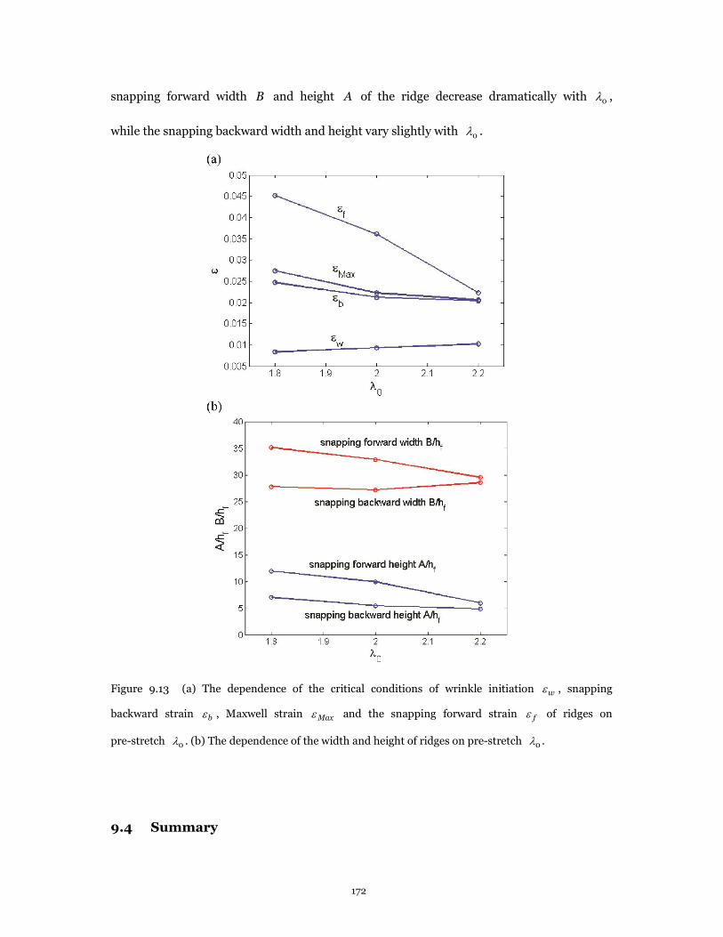
172

snapping forward width B and height A of the ridge decrease dramatically with 0l ,

while the snapping backward width and height vary slightly with 0l .

Figure 9.13 (a) The dependence of the critical conditions of wrinkle initiation we , snapping

backward strain be , Maxwell strain Maxe and the snapping forward strain fe of ridges on

pre-stretch 0l . (b) The dependence of the width and height of ridges on pre-stretch 0l .

9.4 Summary

173

In this chapter, we study the mechanics of the formation and propagation of localized

ridge instability by finite element analysis. Subject to a critical compression, a film/substrate

bilayer with substrate under high tensile pre-stretch forms wrinkles first. With the further

increase of the compression, wrinkles can transit to localized ridges by lifting up the peaks in

every several wrinkles. The wrinkle to ridge transition is subcritical — that is unstable, and

wrinkles dynamically snap to ridges. We develop two numerical ways to study ridges: static

force-displacement method and pseudo-dynamic loading-unloading method. We can obtain

all the stable equilibrium solutions to the boundary value problem under different given

strain by both methods. Therefore, we can find the snapping backward strain be , the

Maxwell strain Maxe and the snapping forward strain fe of ridges. We further analyze the

strain and energy distributions of the wrinkle and ridge states in order to understand the

deformation mechanism of ridges. We find that under a sufficiently large strain the ridge

state reduced the energy in both the film and substrate compared to the wrinkle state. Ridges

have a high aspect ratio, which facilitates their applications in reversible control of

wettability and adhesion.

174

Chapter 10

Conclusions

Mechanical instabilities are ubiquitous in nature and daily life. In the engineering

field, mechanical instabilities were thought to be failure modes of materials, but now people

start to develop various creative applications of mechanical instabilities. Moreover, because

of the high stretchability of soft materials, new types of highly nonlinear instabilities were

realized.

Motivated by this emerging field, this thesis has explored different types of

mechanical instabilities: creases, wrinkles, folds, and ridges. This thesis has studied

mechanical instabilities in materials with different properties and structures, proposed

understandings of the deformation mechanisms of different types of mechanical instabilities,

designed structures to realize a better control of the formation and disappearance of

mechanical instabilities, and shown new types of mechanical instabilities.

We started with studying creases in homogeneous materials. We first studied creases

in soft tissues generated by constrained growth. We adopted the model of growth that factors

the deformation gradient into a growth tensor and an elastic deformation tensor, and

showed that the critical conditions for the onset of creases take a remarkably simple form.

The critical conditions were illustrated with tubes of tissues growing either inside a rigid

shell or outside a rigid core. Furthermore, deep creases in a tube of tissues were simulated by

using the finite element method, and the number of creases in the tube was estimated by

minimizing the free energy. We then studied creases in strain-stiffening materials by the

175

finite element method. We found that for a solid that stiffens steeply at large strains, as the

compression increases, the surface is initially smooth, then forms creases, and finally

becomes smooth again. For a solid that stiffens steeply at small strains, creases never form

and the surface remains smooth for all levels of compression. We also obtained the critical

conditions for the formation of wrinkles in strain-stiffening materials by a linear

perturbation method. When the surface does become unstable, we find that creases always

set in at a lower compression than wrinkles. Our findings may shed light in developing

crease-resistant materials.

Since the conditions for the formation and disappearance of creases had so far been

poorly controlled, we then designed a soft elastic bilayer, with similar moduli of the two

layers but the substrate pre-compressed, and showed that it can snap between the flat and

creased states repeatedly, with hysteresis. The strains at which the creases form and

disappear are highly reproducible, and are tunable over a large range, through variations in

the level of pre-compression applied to the substrate and the thickness ratio of the two layers.

We conducted both numerical simulations and experiments, and showed that they agree very

well with each other. The introduction of bistable flat and creased states and hysteretic

switching is an important step to enable applications of crease instability.

Next we showed that an interface between two soft materials under compression can

form creases, a type of bifurcation distinct from wrinkles. While creases bifurcate from a

state of flat interface by a deformation localized in space and large in amplitude, wrinkles

bifurcate from a state of flat interface by a deformation nonlocal in space and infinitesimal in

amplitude. The interfacial creases set in at a lower critical compression than interfacial

176

wrinkles, but higher than surface creases. The condition for the onset of interfacial creases is

scale-free, and was calculated in terms of elastic moduli, pre-strains and applied strains. Our

experimental observations verified the theoretical predictions.

Then we studied the formation of wrinkles or creases in bilayers. We constructed a

diagram of the formation of wrinkles and creases in a bilayer, and found several new types of

bifurcation behavior when the moduli and the thicknesses of the film and substrate are

comparable. We studied initiation of wrinkles by the linear perturbation method and

initiation and growth of creases by the finite element method. We found creases tend to set

in for more compliant and thicker films, while wrinkles tend to set in for stiffer and thinner

films. When the modulus ratio of the film to substrate is smaller than a critical value 1.65,

creases always form earlier than wrinkles. When the film and substrate have comparable

moduli, creases could be subcritical or supercritical. Creases can also form from wrinkles by

channeling at a much lower strain than the critical strain for the onset of creases in a

homogeneous material.

We further studied the post-wrinkling bifurcations. We demonstrated that

pre-stretched substrates not only show substantial shifts in the critical strain for the onset of

post-wrinkling bifurcations, but also exhibit qualitatively different post-wrinkled states. In

particular, we reported on the stabilization of wrinkles in films on pre-tensioned substrates

and the emergence of ‘chaotic’ morphologies in films on pre-compressed substrates.

When the pre-stretch in the substrate is a sufficiently large tensile stretch, we

demonstrated a different type of post-wrinkling bifurcation, localized ridges. The evolution

of ridge localizations and networks was realized by incremental release of a large equi-biaxial

177

substrate pre-stretch in a microfluidic device. We found the wrinkle to ridge transition is

subcritical. Ridges only form when the equi-biaxial pre-stretch is larger than 1.4. We further

studied the mechanics of ridge formation and propagation. We developed two numerical

ways to study ridges: static force-displacement method and pseudo-dynamic

loading-unloading method, both of which allow us to find all the stable equilibrium solutions

to the boundary value problem under different given strains, including the flat, wrinkle and

ridge states. We obtained the snapping forward strain, snapping backward strain, and

Maxwell strain of wrinkle to ridge transitions. We found the formation of a localized ridge

can reduce the energy in both the film and substrate compared to the wrinkle state by

protruding the surface out and releasing the pre-tension in the substrate.

Mechanical instability in soft materials is an emerging field. It is hoped that this

thesis provides insight into the fundamental understanding of the different types of

instability modes and contributes to the new applications of mechanical instabilities.

178

Bibliography

[1] E. Sharon, M. Marder, H. L. Swinney, Leaves, flowers and garbage bags: Making waves,

American Scientist, 2004, 92 (3): 254-261.

[2] H. Vandeparre, M. Pineirua, F. Brau, B. Roman, J. Bico, C. Gay, W. Z. Bao, C. N. Lau, P.

M. Reis, P. Damman, Wrinkling hierarchy in constrained thin sheets from suspended

graphene to curtains, Physical Review Letters, 2011, 106 (22): 224301.

[3] B. Li, Y. P. Cao, X. Q. Feng, H. J. Gao, Mechanics of morphological instabilities and

surface wrinkling in soft materials: A review, Soft Matter, 2012, 8 (21): 5728-5745.

[4] H. Vandeparre, S. Gabriele, F. Brau, C. Gay, K. K. Parker, P. Damman, Hierarchical

wrinkling patterns, Soft Matter, 2010, 6 (22): 5751-5756.

[5] E. Chater, J. W. Hutchinson, On the propagation of bulges and buckles, Journal of

Applied Mechanics-Transactions of the ASME, 1984, 51 (2): 269-277.

[6] S. Krylov, B. R. Ilic, D. Schreiber, S. Seretensky, H. Craighead, The pull-in behavior of

electrostatically actuated bistable microstructures, Journal of Micromechanics and

Microengineering, 2008, 18 (5): 055026.

[7] Y. Hu, A. Hiltner, E. Baer, Buckling in elastomer/plastic/elastomer 3-layer films,

Polymer Composites, 2004, 25 (6): 653-661.

[8] S. Yang, K. Khare, P. C. Lin, Harnessing surface wrinkle patterns in soft matter,

Advanced Functional Materials, 2010, 20 (16): 2550-2564.

[9] C. M. Chen, S. Yang, Wrinkling instabilities in polymer films and their applications,

Polymer International, 2012, 61 (7): 1041-1047.

179

[10] J. Genzer, J. Groenewold, Soft matter with hard skin: From skin wrinkles to

templating and material characterization, Soft Matter, 2006, 2 (4): 310-323.

[11] E. P. Chan, A. J. Crosby, Fabricating microlens arrays by surface wrinkling, Advanced

Materials, 2006, 18 (24): 3238-3242.

[12] X. Chen, J. Yin, Buckling patterns of thin films on curved compliant substrates with

applications to morphogenesis and three-dimensional micro-fabrication, Soft Matter,

2010, 6 (22): 5667-5680.

[13] D. Y. Khang, H. Q. Jiang, Y. Huang, J. A. Rogers, A stretchable form of single-crystal

silicon for high-performance electronics on rubber substrates, Science, 2006, 311

(5758): 208-212.

[14] D. Y. Khang, J. A. Rogers, H. H. Lee, Mechanical buckling: Mechanics, metrology, and

stretchable electronics, Advanced Functional Materials, 2009, 19 (10): 1526-1536.

[15] S. Lee, S. Kim, T. T. Kim, Y. Kim, M. Choi, S. H. Lee, J. Y. Kim, B. Min, Reversibly

stretchable and tunable terahertz metamaterials with wrinkled layouts, Advanced

Materials, 2012, 24 (26): 3491-3497.

[16] D. J. Lipomi, B. C. K. Tee, M. Vosgueritchian, Z. N. Bao, Stretchable organic solar cells,

Advanced Materials, 2011, 23 (15): 1771-1775.

[17] M. S. White, M. Kaltenbrunner, E. D. Glowacki, K. Gutnichenko, G. Kettlgruber, I.

Graz, S. Aazou, C. Ulbricht, D. A. M. Egbe, M. C. Miron, Z. Major, M. C. Scharber, T.

Sekitani, T. Someya, S. Bauer, N. S. Sariciftci, Ultrathin, highly flexible and stretchable

pleds, Nature Photonics, 2013, 7 (10): 811-816.

[18] J. B. Kim, P. Kim, N. C. Pegard, S. J. Oh, C. R. Kagan, J. W. Fleischer, H. A. Stone, Y. L.

180

Loo, Wrinkles and deep folds as photonic structures in photovoltaics, Nature Photonics,

2012, 6 (5): 327-332.

[19] Y. F. Mei, D. J. Thurmer, F. Cavallo, S. Kiravittaya, O. G. Schmidt, Semiconductor

sub-micro-/nanochannel networks by deterministic layer wrinkling, Advanced

Materials, 2007, 19 (16): 2124-2128.

[20] S. Chung, J. H. Lee, M. W. Moon, J. Han, R. D. Kamm, Non-lithographic wrinkle

nanochannels for protein preconcentration, Advanced Materials, 2008, 20 (16):

3011-3016.

[21] K. Khare, J. H. Zhou, S. Yang, Tunable open-channel microfluidics on soft

poly(dimethylsiloxane) (PDMS) substrates with sinusoidal grooves, Langmuir, 2009,

25 (21): 12794-12799.

[22] C. M. Stafford, C. Harrison, K. L. Beers, A. Karim, E. J. Amis, M. R. Vanlandingham, H.

C. Kim, W. Volksen, R. D. Miller, E. E. Simonyi, A buckling-based metrology for

measuring the elastic moduli of polymeric thin films, Nature Materials, 2004, 3 (8):

545-550.

[23] J. Y. Chung, A. J. Nolte, C. M. Stafford, Surface wrinkling: A versatile platform for

measuring thin-film properties, Advanced Materials, 2011, 23 (3): 349-368.

[24] E. A. Wilder, S. Guo, S. Lin-Gibson, M. J. Fasolka, C. M. Stafford, Measuring the

modulus of soft polymer networks via a buckling-based metrology, Macromolecules,

2006, 39 (12): 4138-4143.

[25] J. Huang, M. Juszkiewicz, W. H. de Jeu, E. Cerda, T. Emrick, N. Menon, T. P. Russell,

Capillary wrinkling of floating thin polymer films, Science, 2007, 317 (5838): 650-653.

181

[26] J. A. Howarter, C. M. Stafford, Instabilities as a measurement tool for soft materials,

Soft Matter, 2010, 6 (22): 5661-5666.

[27] C. H. Lu, H. Mohwald, A. Fery, A lithography-free method for directed colloidal crystal

assembly based on wrinkling, Soft Matter, 2007, 3 (12): 1530-1536.

[28] A. Schweikart, A. Fery, Controlled wrinkling as a novel method for the fabrication of

patterned surfaces, Microchimica Acta, 2009, 165 (3-4): 249-263.

[29] A. Chen, D. K. Lieu, L. Freschauf, V. Lew, H. Sharma, J. X. Wang, D. Nguyen, I.

Karakikes, R. J. Hajjar, A. Gopinathan, E. Botvinick, C. C. Fowlkes, R. A. Li, M. Khine,

Shrink-film configurable multiscale wrinkles for functional alignment of human

embryonic stem cells and their cardiac derivatives, Advanced Materials, 2011, 23 (48):

5785-5791.

[30] M. Guvendiren, J. A. Burdick, Stem cell response to spatially and temporally displayed

and reversible surface topography, Advanced Healthcare Materials, 2013, 2 (1):

155-164.

[31] P. C. Lin, S. Vajpayee, A. Jagota, C. Y. Hui, S. Yang, Mechanically tunable dry adhesive

from wrinkled elastomers, Soft Matter, 2008, 4 (9): 1830-1835.

[32] E. P. Chan, E. J. Smith, R. C. Hayward, A. J. Crosby, Surface wrinkles for smart

adhesion, Advanced Materials, 2008, 20 (4): 711-716.

[33] Y. Rahmawan, C.-M. Chen, S. Yang, Recent advances in wrinkle-based dry adhesion,

Soft Matter, 2014, 10 (28): 5028–5039.

[34] J. Y. Chung, J. P. Youngblood, C. M. Stafford, Anisotropic wetting on tunable

micro-wrinkled surfaces, Soft Matter, 2007, 3 (9): 1163-1169.

182

[35] P. C. Lin, S. Yang, Mechanically switchable wetting on wrinkled elastomers with

dual-scale roughness, Soft Matter, 2009, 5 (5): 1011-1018.

[36] D. Y. Xia, L. M. Johnson, G. P. Lopez, Anisotropic wetting surfaces with

one-dimesional and directional structures: Fabrication approaches, wetting properties

and potential applications, Advanced Materials, 2012, 24 (10): 1287-1302.

[37] S. G. Lee, D. Y. Lee, H. S. Lim, D. H. Lee, S. Lee, K. Cho, Switchable transparency and

wetting of elastomeric smart windows, Advanced Materials, 2010, 22 (44): 5013-5017.

[38] C. J. Rand, A. J. Crosby, Friction of soft elastomeric wrinkled surfaces, Journal of

Applied Physics, 2009, 106 (6): 064913.

[39] J. Kim, J. Yoon, R. C. Hayward, Dynamic display of biomolecular patterns through an

elastic creasing instability of stimuli-responsive hydrogels, Nature Materials, 2010, 9

(2): 159-164.

[40] P. Kim, Y. H. Hu, J. Alvarenga, M. Kolle, Z. G. Suo, J. Aizenberg, Rational design of

mechano-responsive optical materials by fine tuning the evolution of strain-dependent

wrinkling patterns, Advanced Optical Materials, 2013, 1 (5): 381-388.

[41] E. Lee, M. L. Zhang, Y. Cho, Y. Cui, J. Van der Spiegel, N. Engheta, S. Yang, Tilted

pillars on wrinkled elastomers as a reversibly tunable optical window, Advanced

Materials, 2014, 26 (24): 4127-4133.

[42] B. Kolaric, H. Vandeparre, S. Desprez, R. A. L. Vallee, P. Damman, In situ tuning the

optical properties of a cavity by wrinkling, Applied Physics Letters, 2010, 96 (4):

043119.

[43] D. P. Holmes, A. J. Crosby, Snapping surfaces, Advanced Materials, 2007, 19 (21):

183

3589-3593.

[44] M. Basan, J. F. Joanny, J. Prost, T. Risler, Undulation instability of epithelial tissues,

Physical Review Letters, 2011, 106 (15): 158101.

[45] B. Li, F. Jia, Y. P. Cao, X. Q. Feng, H. J. Gao, Surface wrinkling patterns on a core-shell

soft sphere, Physical Review Letters, 2011, 106 (23): 234301.

[46] A. Goriely, R. Vandiver, On the mechanical stability of growing arteries, IMA Journal

of Applied Mathematics, 2010, 75 (4): 549-570.

[47] Y. Forterre, J. M. Skotheim, J. Dumais, L. Mahadevan, How the venus flytrap snaps,

Nature, 2005, 433 (7024): 421-425.

[48] L. Jin, S. Cai, Z. Suo, Creases in soft tissues generated by growth, Europhysics Letters,

2011, 95 (6): 64002.

[49] M. A. Wyczalkowski, Z. Chen, B. A. Filas, V. D. Varner, L. A. Taber, Computational

models for mechanics of morphogenesis, Birth Defects Research Part C-Embryo

Today-Reviews, 2012, 96 (2): 132-152.

[50] M. Kucken, A. C. Newell, A model for fingerprint formation, Europhysics Letters,

2004, 68 (1): 141-146.

[51] L. Pauchard, Y. Couder, Invagination during the collapse of an inhomogeneous

spheroidal shell, Europhysics Letters, 2004, 66 (5): 667-673.

[52] T. Savin, N. A. Kurpios, A. E. Shyer, P. Florescu, H. Y. Liang, L. Mahadevan, C. J.

Tabin, On the growth and form of the gut, Nature, 2011, 476 (7358): 57-62.

[53] E. Hannezo, J. Prost, J. F. Joanny, Instabilities of monolayered epithelia: Shape and

structure of villi and crypts, Physical Review Letters, 2011, 107 (7): 078104.

184

[54] A. E. Shyer, T. Tallinen, N. L. Nerurkar, Z. Y. Wei, E. S. Gil, D. L. Kaplan, C. J. Tabin, L.

Mahadevan, Villification: How the gut gets its villi, Science, 2013, 342 (6155): 212-218.

[55] M. Ben Amar, F. Jia, Anisotropic growth shapes intestinal tissues during

embryogenesis, Proceedings of the National Academy of Sciences of the United States

of America, 2013, 110 (26): 10525-10530.

[56] D. P. Richman, R. M. Stewart, J. W. Hutchinson, V. S. Caviness, Mechanical model of

brain convolutional development, Science, 1975, 189 (4196): 18-21.

[57] S. Budday, C. Raybaud, E. Kuhl, A mechanical model predicts morphological

abnormalities in the developing human brain, Scientific reports, 2014, 4 5644.

[58] P. V. Bayly, L. A. Taber, C. D. Kroenke, Mechanical forces in cerebral cortical folding:

A review of measurements and models, Journal of the Mechanical Behavior of

Biomedical Materials, 2014, 29 568-581.

[59] M. Ben Amar, C. Chatelain, P. Ciarletta, Contour instabilities in early tumor growth

models, Physical Review Letters, 2011, 106 (14): 148101.

[60] W. Yang, T. C. Fung, K. S. Chian, C. K. Chong, Instability of the two-layered

thick-walled esophageal model under the external pressure and circular outer

boundary condition, Journal of Biomechanics, 2007, 40 (3): 481-490.

[61] B. Li, Y. P. Cao, X. Q. Feng, S. W. Yu, Mucosal wrinkling in animal antra induced by

volumetric growth, Applied Physics Letters, 2011, 98 (15): 153701.

[62] B. Li, Y. P. Cao, X. Q. Feng, H. J. Gao, Surface wrinkling of mucosa induced by

volumetric growth: Theory, simulation and experiment, Journal of the Mechanics and

Physics of Solids, 2011, 59 (4): 758-774.

185

[63] D. E. Moulton, A. Goriely, Possible role of differential growth in airway wall

remodeling in asthma, Journal of Applied Physiology, 2011, 110 (4): 1003-1012.

[64] J. Lidmar, L. Mirny, D. R. Nelson, Virus shapes and buckling transitions in spherical

shells, Physical Review E, 2003, 68 (5): 051910.

[65] J. Dumais, C. R. Steele, New evidence for the role of mechanical forces in the shoot

apical meristem, Journal of Plant Growth Regulation, 2000, 19 (1): 7-18.

[66] H. Y. Liang, L. Mahadevan, The shape of a long leaf, Proceedings of the National

Academy of Sciences of the United States of America, 2009, 106 (52): 22049-22054.

[67] H. Y. Liang, L. Mahadevan, Growth, geometry, and mechanics of a blooming lily,

Proceedings of the National Academy of Sciences of the United States of America,

2011, 108 (14): 5516-5521.

[68] S. Armon, E. Efrati, R. Kupferman, E. Sharon, Geometry and mechanics in the

opening of chiral seed pods, Science, 2011, 333 (6050): 1726-1730.

[69] P. D. Shipman, A. C. Newell, Phyllotactic patterns on plants, Physical Review Letters,

2004, 92 (16): 168102.

[70] J. Dervaux, M. Ben Amar, Morphogenesis of growing soft tissues, Physical Review

Letters, 2008, 101 (6): 068101.

[71] E. Katifori, S. Alben, E. Cerda, D. R. Nelson, J. Dumais, Foldable structures and the

natural design of pollen grains, Proceedings of the National Academy of Sciences of

the United States of America, 2010, 107 (17): 7635-7639.

[72] J. Yin, Z. X. Cao, C. R. Li, I. Sheinman, X. Chen, Stress-driven buckling patterns in

spheroidal core/shell structures, Proceedings of the National Academy of Sciences of

186

the United States of America, 2008, 105 (49): 19132-19135.

[73] E. Hohlfeld, Creasing, post-bifurcations and the spontaneous breakdown of scale

invariance, PhD thesis, Harvard University, Cambridge, MA, 2008.

[74] L. Pocivavsek, R. Dellsy, A. Kern, S. Johnson, B. H. Lin, K. Y. C. Lee, E. Cerda, Stress

and fold localization in thin elastic membranes, Science, 2008, 320 (5878): 912-916.

[75] Y. P. Cao, J. W. Hutchinson, Wrinkling phenomena in neo-hookean film/substrate

bilayers, Journal of Applied Mechanics-Transactions of the ASME, 2012, 79 (3):

031019.

[76] E. Cerda, L. Mahadevan, Geometry and physics of wrinkling, Physical Review Letters,

2003, 90 (7): 074302.

[77] Z. Y. Huang, W. Hong, Z. Suo, Nonlinear analyses of wrinkles in a film bonded to a

compliant substrate, Journal of the Mechanics and Physics of Solids, 2005, 53 (9):

2101-2118.

[78] X. Chen, J. W. Hutchinson, Herringbone buckling patterns of compressed thin films

on compliant substrates, Journal of Applied Mechanics-Transactions of the ASME,

2004, 71 (5): 597-603.

[79] K. D. Danov, P. A. Kralchevsky, S. D. Stoyanov, Elastic langmuir layers and

membranes subjected to unidirectional compression: Wrinkling and collapse,

Langmuir, 2010, 26 (1): 143-155.

[80] K. Efimenko, M. Rackaitis, E. Manias, A. Vaziri, L. Mahadevan, J. Genzer, Nested

self-similar wrinkling patterns in skins, Nature Materials, 2005, 4 (4): 293-297.

[81] N. Bowden, S. Brittain, A. G. Evans, J. W. Hutchinson, G. M. Whitesides, Spontaneous

187

formation of ordered structures in thin films of metals supported on an elastomeric

polymer, Nature, 1998, 393 (6681): 146-149.

[82] S. Cai, D. Breid, A. J. Crosby, Z. Suo, J. W. Hutchinson, Periodic patterns and energy

states of buckled films on compliant substrates, Journal of the Mechanics and Physics

of Solids, 2011, 59 (5): 1094-1114.

[83] D. Breid, A. J. Crosby, Effect of stress state on wrinkle morphology, Soft Matter, 2011,

7 (9): 4490-4496.

[84] J. Yin, J. L. Yague, D. Eggenspieler, K. K. Gleason, M. C. Boyce, Deterministic order in

surface micro-topologies through sequential wrinkling, Advanced Materials, 2012, 24

(40): 5441-5446.

[85] B. Audoly, A. Boudaoud, Buckling of a stiff film bound to a compliant substrate - Part I:

Formulation, linear stability of cylindrical patterns, secondary bifurcations, Journal of

the Mechanics and Physics of Solids, 2008, 56 (7): 2401-2421.

[86] P.-C. Lin, S. Yang, Spontaneous formation of one-dimensional ripples in transit to

highly ordered two-dimensional herringbone structures through sequential and

unequal biaxial mechanical stretching, Applied Physics Letters, 2007, 90 (24): 241903.

[87] E. Cerda, K. Ravi-Chandar, L. Mahadevan, Thin films - wrinkling of an elastic sheet

under tension, Nature, 2002, 419 (6907): 579-580.

[88] A. Takei, F. Brau, B. Roman, J. Bico, Stretch-induced wrinkles in reinforced

membranes: From out-of-plane to in-plane structures, Europhysics Letters, 2011, 96

(6): 64001.

[89] V. Nayyar, K. Ravi-Chandar, R. Huang, Stretch-induced stress patterns and wrinkles

188

in hyperelastic thin sheets, International Journal of Solids and Structures, 2011, 48

(25-26): 3471-3483.

[90] A. L. Volynskii, S. Bazhenov, O. V. Lebedeva, N. F. Bakeev, Mechanical buckling

instability of thin coatings deposited on soft polymer substrates, Journal of Materials

Science, 2000, 35 (3): 547-554.

[91] Y. W. Wong, S. Pellegrino, Wrinkled membranes Part I: Experiments, Journal of

Mechanics of Materials and Structures, 2006, 1 (1): 3-25.

[92] P. Ciarletta, M. Destrade, A. L. Gower, Shear instability in skin tissue, Quarterly

Journal of Mechanics and Applied Mathematics, 2013, 66 (2): 273-288.

[93] M. Destrade, M. D. Gilchrist, J. A. Motherway, J. G. Murphy, Bimodular rubber

buckles early in bending, Mechanics of Materials, 2010, 42 (4): 469-476.

[94] M. Destrade, A. N. Annaidh, C. D. Coman, Bending instabilities of soft biological

tissues, International Journal of Solids and Structures, 2009, 46 (25-26): 4322-4330.

[95] J. Y. Sun, S. M. Xia, M. W. Moon, K. H. Oh, K. S. Kim, Folding wrinkles of a thin stiff

layer on a soft substrate, Proceedings of the Royal Society A-Mathematical Physical

and Engineering Sciences, 2012, 468 (2140): 932-953.

[96] J. L. Nowinski, Surface instability of a half-space under high two-dimensional

compression, Journal of the Franklin Institute, 1969, 288 (5): 367-376.

[97] M. A. Biot, Surface instability of rubber in compression, Applied Scientific Research,

1963, 12 168-182.

[98] M. A. Biot, Mechanics of incremental deformations, John Wiley & Sons, New York,

1965.

189

[99] Q. M. Wang, X. H. Zhao, Phase diagrams of instabilities in compressed film-substrate

systems, Journal of Applied Mechanics-Transactions of the ASME, 2013, 81 (5):

051004.

[100] M. A. Biot, Interfacial instability in finite elsticity under initial stress, Proceedings of

the Royal Society A-Mathematical Physical and Engineering Sciences, 1963, 273

(1352): 340-344.

[101] J. Groenewold, Wrinkling of plates coupled with soft elastic media, Physica A, 2001,

298 (1-2): 32-45.

[102] H. Q. Jiang, D. Y. Khang, J. Z. Song, Y. G. Sun, Y. G. Huang, J. A. Rogers, Finite

deformation mechanics in buckled thin films on compliant supports, Proceedings of

the National Academy of Sciences of the United States of America, 2007, 104 (40):

15607-15612.

[103] J. Song, H. Jiang, Z. J. Liu, D. Y. Khang, Y. Huang, J. A. Rogers, C. Lu, C. G. Koh,

Buckling of a stiff thin film on a compliant substrate in large deformation,

International Journal of Solids and Structures, 2008, 45 (10): 3107-3121.

[104] B. Li, S. Q. Huang, X. Q. Feng, Buckling and postbuckling of a compressed thin film

bonded on a soft elastic layer: A three-dimensional analysis, Archive of Applied

Mechanics, 2010, 80 (2): 175-188.

[105] A. N. Gent, I. S. Cho, Surface instabilities in compressed or bent rubber blocks,

Rubber Chemistry and Technology, 1999, 72 (2): 253-262.

[106] E. Hohlfeld, L. Mahadevan, Unfolding the sulcus, Physical Review Letters, 2011, 106

(10): 105702.

190

[107] W. Hong, X. H. Zhao, Z. G. Suo, Formation of creases on the surfaces of elastomers

and gels, Applied Physics Letters, 2009, 95 (11): 111901.

[108] S. Q. Cai, K. Bertoldi, H. M. Wang, Z. G. Suo, Osmotic collapse of a void in an

elastomer: Breathing, buckling and creasing, Soft Matter, 2010, 6 (22): 5770-5777.

[109] W. H. Wong, T. F. Guo, Y. W. Zhang, L. Cheng, Surface instability maps for soft

materials, Soft Matter, 2010, 6 (22): 5743-5750.

[110] T. Tallinen, J. S. Biggins, L. Mahadevan, Surface sulci in squeezed soft solids,

Physical Review Letters, 2013, 110 (2): 024302.

[111] W. Hong, F. Gao, Crease instability on the surface of a solid, in: X. Chen (Ed.)

Mechanical self-assembly, Springer, New York, 2013, 111-130.

[112] V. Trujillo, J. Kim, R. C. Hayward, Creasing instability of surface-attached hydrogels,

Soft Matter, 2008, 4 (3): 564-569.

[113] S. Q. Cai, D. Y. Chen, Z. G. Suo, R. C. Hayward, Creasing instability of elastomer films,

Soft Matter, 2012, 8 (5): 1301-1304.

[114] A. Ghatak, A. L. Das, Kink instability of a highly deformable elastic cylinder, Physical

Review Letters, 2007, 99 (7): 076101.

[115] S. Mora, M. Abkarian, H. Tabuteau, Y. Pomeau, Surface instability of soft solids under

strain, Soft Matter, 2011, 7 (22): 10612-10619.

[116] B. Xu, D. Chen, R. C. Hayward, Mechanically gated electrical switches by creasing of

patterned metal/elastomer bilayer films, Advanced Materials, 2014, 26 (25):

4381-4385.

[117] T. Tanaka, Kinetics of phase transition in polymer gels, Physica A, 1986, 140 (1-2):

191

261-268.

[118] T. Tanaka, S. T. Sun, Y. Hirokawa, S. Katayama, J. Kucera, Y. Hirose, T. Amiya,

Mechanical instability of gels at the phase transition, Nature, 1987, 325 (6107):

796-798.

[119] J. Yoon, J. Kim, R. C. Hayward, Nucleation, growth, and hysteresis of surface creases

on swelled polymer gels, Soft Matter, 2010, 6 (22): 5807-5816.

[120] M. Guvendiren, J. A. Burdick, S. Yang, Solvent induced transition from wrinkles to

creases in thin film gels with depth-wise crosslinking gradients, Soft Matter, 2010, 6

(22): 5795-5801.

[121] O. Ortiz, A. Vidyasagar, J. Wang, R. Toomey, Surface instabilities in ultrathin,

cross-linked poly(n-isopropylacrylamide) coatings, Langmuir, 2010, 26 (22):

17489-17494.

[122] J. Dervaux, Y. Couder, M. A. Guedeau-Boudeville, M. Ben Amar, Shape transition in

artificial tumors: From smooth buckles to singular creases, Physical Review Letters,

2011, 107 (1): 018103.

[123] J. Dervaux, M. Ben Amar, Mechanical instabilities of gels, Annual Review of

Condensed Matter Physics, 2012, 3 311-332.

[124] M. Arifuzzaman, Z. L. Wu, T. Kurokawa, A. Kakugo, J. P. Gong, Swelling-induced

long-range ordered structure formation in polyelectrolyte hydrogel, Soft Matter, 2012,

8 (31): 8060-8066.

[125] W. Barros, E. N. de Azevedo, M. Engelsberg, Surface pattern formation in a swelling

gel, Soft Matter, 2012, 8 (32): 8511-8516.

192

[126] A. Pandey, D. P. Holmes, Swelling-induced deformations: A materials-defined

transition from macroscale to microscale deformations, Soft Matter, 2013, 9 (23):

5524-5528.

[127] F. Weiss, S. Cai, Y. Hu, M. K. Kang, R. Huang, Z. Suo, Creases and wrinkles on the

surface of a swollen gel, Journal of Applied Physics, 2013, 114 073507.

[128] N. Zalachas, S. Q. Cai, Z. G. Suo, Y. Lapusta, Crease in a ring of a pH-sensitive

hydrogel swelling under constraint, International Journal of Solids and Structures,

2013, 50 (6): 920-927.

[129] J. Kim, Morphological analysis of crease patterns formed on surface-attached

hydrogel with a gradient in thickness, Journal of Applied Polymer Science, 2014, 131

(13): 40482.

[130] Q. M. Wang, L. Zhang, X. H. Zhao, Creasing to cratering instability in polymers

under ultrahigh electric fields, Physical Review Letters, 2011, 106 (11): 118301.

[131] Q. M. Wang, X. F. Niu, Q. B. Pei, M. D. Dickey, X. H. Zhao, Electromechanical

instabilities of thermoplastics: Theory and in situ observation, Applied Physics Letters,

2012, 101 (14): 141911.

[132] Q. M. Wang, X. H. Zhao, Creasing-wrinkling transition in elastomer films under

electric fields, Physical Review E, 2013, 88 (4): 042403.

[133] H. S. Park, Q. M. Wang, X. H. Zhao, P. A. Klein, Electromechanical instability on

dielectric polymer surface: Modeling and experiment, Computer Methods in Applied

Mechanics and Engineering, 2013, 260 40-49.

[134] B. Xu, R. C. Hayward, Low-voltage switching of crease patterns on hydrogel surfaces,

193

Advanced Materials, 2013, 25 (39): 5555-5559.

[135] Q. Wang, D. Robinson, X. Zhao, On-demand hierarchical patterning with electric

fields, Applied Physics Letters, 2014, 104 (23): 231605.

[136] J. Yoon, P. Bian, J. Kim, T. J. McCarthy, R. C. Hayward, Local switching of chemical

patterns through light-triggered unfolding of creased hydrogel surfaces, Angewandte

Chemie-international Edition, 2012, 51 (29): 7146-7149.

[137] P. Gabriel, Y. Fukahori, A. G. Thomas, J. J. C. Busfield, FEA modeling of schallamach

waves, Rubber Chemistry and Technology, 2010, 83 (4): 358-367.

[138] D. Y. Chen, S. Q. Cai, Z. G. Suo, R. C. Hayward, Surface energy as a barrier to

creasing of elastomer films: An elastic analogy to classical nucleation, Physical Review

Letters, 2012, 109 (3): 038001.

[139] E. Hohlfeld, L. Mahadevan, Scale and nature of sulcification patterns, Physical

Review Letters, 2012, 109 (2): 025701.

[140] L. Jin, D. Chen, R. C. Hayward, Z. Suo, Creases on the interface between two soft

materials, Soft Matter, 2014, 10 (2): 303-311.

[141] K. Saha, J. Kim, E. Irwin, J. Yoon, F. Momin, V. Trujillo, D. V. Schaffer, K. E. Healy, R.

C. Hayward, Surface creasing instability of soft polyacrylamide cell culture substrates,

Biophysical Journal, 2010, 99 (12): 94-96.

[142] E. P. Chan, J. M. Karp, R. S. Langer, A "self-pinning" adhesive based on responsive

surface wrinkles, Journal of Polymer Science Part B-Polymer Physics, 2011, 49 (1):

40-44.

[143] P. Shivapooja, Q. Wang, B. Orihuela, D. Rittschof, G. P. Lopez, X. Zhao, Bioinspired

194

surfaces with dynamic topography for active control of biofouling, Advanced Materials,

2013, 25 (10): 1430-1434.

[144] L. Pocivavsek, B. Leahy, N. Holten-Andersen, B. Lin, K. Y. C. Lee, E. Cerda,

Geometric tools for complex interfaces: From lung surfactant to the mussel byssus, Soft

Matter, 2009, 5 (10): 1963-1968.

[145] F. Brau, H. Vandeparre, A. Sabbah, C. Poulard, A. Boudaoud, P. Damman,

Multiple-length-scale elastic instability mimics parametric resonance of nonlinear

oscillators, Nature Physics, 2011, 7 (1): 56-60.

[146] P. Kim, M. Abkarian, H. A. Stone, Hierarchical folding of elastic membranes under

biaxial compressive stress, Nature Materials, 2011, 10 (12): 952-957.

[147] F. Brau, P. Damman, H. Diamant, T. A. Witten, Wrinkle to fold transition: Influence

of the substrate response, Soft Matter, 2013, 9 (34): 8177-8186.

[148] Y. Ebata, A. B. Croll, A. J. Crosby, Wrinkling and strain localizations in polymer thin

films, Soft Matter, 2012, 8 (35): 9086-9091.

[149] B. Audoly, Localized buckling of a floating elastica, Physical Review E, 2011, 84 (1):

011605.

[150] A. B. Croll, A. J. Crosby, Pattern driven stress localization in thin diblock copolymer

films, Macromolecules, 2012, 45 (9): 4001-4006.

[151] D. P. Holmes, A. J. Crosby, Draping films: A wrinkle to fold transition, Physical

Review Letters, 2010, 105 (3): 038303.

[152] B. D. Leahy, L. Pocivavsek, M. Meron, K. L. Lam, D. Salas, P. J. Viccaro, K. Y. C. Lee,

B. Lin, Geometric stability and elastic response of a supported nanoparticle film,

195

Physical Review Letters, 2010, 105 (5): 058301.

[153] P. M. Reis, F. Corson, A. Boudaoud, B. Roman, Localization through surface folding

in solid foams under compression, Physical Review Letters, 2009, 103 (4): 045501.

[154] H. Diamant, T. A. Witten, Compression induced folding of a sheet: An integrable

system, Physical Review Letters, 2011, 107 (16): 164302.

[155] J. Zang, X. Zhao, Y. Cao, J. W. Hutchinson, Localized ridge wrinkling of stiff films on

compliant substrates, Journal of the Mechanics and Physics of Solids, 2012, 60 (7):

1265-1279.

[156] C. Cao, H. F. Chan, J. Zang, K. W. Leong, X. Zhao, Harnessing localized ridges for

high-aspect-ratio hierarchical patterns with dynamic tunability and multifunctionality,

Advanced Materials, 2014, 26 (11): 1763-1770.

[157] A. Takei, L. Jin, J. W. Hutchinson, H. Fujita, Ridge localizations and networks in thin

films compressed by the incremental release of a large equi-biaxial pre-stretch in the

substrate, Advanced Materials, 2014, 26 (24): 4061-4067.

[158] Y. C. Chen, A. J. Crosby, High aspect ratio wrinkles via substrate prestretch,

Advanced Materials, 2014, 26 (32): 5626-5631.

[159] B. Li, Y.-P. Cao, X.-Q. Feng, Growth and surface folding of esophageal mucosa: A

biomechanical model, Journal of Biomechanics, 2011, 44 (1): 182-188.

[160] J. Dervaux, M. Ben Amar, Buckling condensation in constrained growth, Journal of

the Mechanics and Physics of Solids, 2011, 59 (3): 538-560.

[161] M. Ben Amar, A. Goriely, Growth and instability in elastic tissues, Journal of the

Mechanics and Physics of Solids, 2005, 53 (10): 2284-2319.

196

[162] B. R. Wiggs, C. A. Hrousis, J. M. Drazen, R. D. Kamm, On the mechanism of mucosal

folding in normal and asthmatic airways, Journal of Applied Physiology, 1997, 83 (6):

1814-1821.

[163] C. A. Hrousis, B. J. R. Wiggs, J. M. Drazen, D. M. Parks, R. D. Kamm, Mucosal

folding in biologic vessels, Journal of Biomechanical Engineering-Transactions of the

ASME, 2002, 124 (4): 334-341.

[164] Y. P. Cao, J. W. Hutchinson, From wrinkles to creases in elastomers: The instability

and imperfection-sensitivity of wrinkling, Proceedings of the Royal Society

A-Mathematical Physical and Engineering Sciences, 2012, 468 (2137): 94-115.

[165] E. K. Rodriguez, A. Hoger, A. D. McCulloch, Stress-dependent finite growth in soft

elastic tissues, Journal of Biomechanics, 1994, 27 (4): 455-467.

[166] R. Skalak, S. Zargaryan, R. K. Jain, P. A. Netti, A. Hoger, Compatibility and the

genesis of residual stress by volumetric growth, Journal of Mathematical Biology,

1996, 34 (8): 889-914.

[167] R. Skalak, Growth as a finite displacement field, in: D.E. Carlson, R.T. Shield (Eds.)

Proceedings of the IUTAM Symposium on Finite Elasticity, Martinus Nijhoff

Publishers, Lehigh University, 1980: 347-355.

[168] D. E. Moulton, A. Goriely, Circumferential buckling instability of a growing

cylindrical tube, Journal of the Mechanics and Physics of Solids, 2011, 59 (3): 525-537.

[169] E. Hohlfeld, Coexistence of scale-invariant states in incompressible elastomers,

Physical Review Letters, 2013, 111 (18): 185701.

[170] J. W. Hutchinson, The role of nonlinear substrate elasticity in the wrinkling of thin

197

films, Philosophical Transactions of the Royal Society A-Mathematical Physical and

Engineering Sciences, 2013, 371 (1993): 20120422.

[171] M. Z. Diab, T. Zhang, R. K. Zhao, H. J. Gao, K. S. Kim, Ruga mechanics of creasing:

From instantaneous to setback creases, Proceedings of the Royal Society

A-Mathematical Physical and Engineering Sciences, 2013, 469 (2157): 20120753.

[172] Z. G. Wu, N. Bouklas, R. Huang, Swell-induced surface instability of hydrogel layers

with material properties varying in thickness direction, International Journal of Solids

and Structures, 2013, 50 (3-4): 578-587.

[173] D. Chen, L. Jin, Z. Suo, R. C. Hayward, Controlled formation and disappearance of

creases, Materials Horizons, 2014, 1 (2): 207-213.

[174] Y. C. Fung, Biomechanics: Material properties of living tissues, Springer, New York

1993.

[175] L. R. G. Treloar, The physics of rubber elasticity (third edition), Clarendon Press,

Oxford, 1975.

[176] A. N. Gent, A new constitutive relation for rubber, Rubber Chemistry and

Technology, 1996, 69 (1): 59-61.

[177] G. A. Holzapfel, Nonlinear solid mechancs: A continuum approach for engineering,

John Wiley & Sons, Chichester, 2000.

[178] A. N. Stroh, Dislocations and cracks in anisotropic elasticity, Philosophical Magazine,

1958, 3 (30): 625-646.

[179] Z. G. Suo, Singularities interfaces and cracks in dissimilar anistropic media,

Proceedings of the Royal Society A-Mathematical Physical and Engineering Sciences,

198

1990, 427 (1873): 331-358.

[180] Z. Suo, M. Ortiz, A. Needleman, Stability of solids with interfaces, Journal of the

Mechanics and Physics of Solids, 1992, 40 (3): 613-640.

[181] G. F. Carrier, M. Krook, C. E. Pearson, Functions of a complex variable: Theory and

technique, Hod Books, Ithaca, 1983.

[182] G. A. Holzapfel, Biomechanics of soft tissue, in: J. Lemaitre (Ed.), The handbook of

materials behavior models, Volume III, Multiphysics behaviors, Academic Press,

Boston, 2001: 1049-1063.

[183] M. G. Dunn, F. H. Silver, D. A. Swann, Mechanical analysis of hypertrophic scar

tissue: Structural basis for apparent increased rigidity, Journal of Investigative

Dermatology, 1985, 84 (1): 9-13.

[184] Y.-L. Pi, M. Bradford, B. Uy, In-plane stability of arches, International Journal of

Solids and Structures, 2002, 39 (1): 105-125.

[185] P. Yang, R. M. Baker, J. H. Henderson, P. T. Mather, In vitro wrinkle formation via

shape memory dynamically aligns adherent cells, Soft Matter, 2013, 9 (18): 4705-4714.

[186] H. Lee, C. Xia, N. X. Fang, First jump of microgel; actuation speed enhancement by

elastic instability, Soft Matter, 2010, 6 (18): 43424345.

[187] C. Keplinger, T. Li, R. Baumgartner, Z. Suo, S. Bauer, Harnessing snap-through

instability in soft dielectrics to achieve giant voltage-triggered deformation, Soft Matter,

2012, 8 (2): 285-288.

[188] Q. Wang, M. Tahir, J. Zang, X. Zhao, Dynamic electrostatic lithography: Multiscale

on-demand patterning on large-area curved surfaces, Advanced Materials, 2012, 24

199

(15): 1947-1951.

[189] E. Riks, The application of newton's method to the problem of elastic stability,

Journal of Applied Mechanics-Transactions of the ASME, 1972, 39 (4): 1060-1065.

[190] J. He, G. H. Xu, Z. Suo, Experimental determination of crack driving forces in

integrated structures, AIP Conference Proceedings, 2004, 741 (1): 3-14.

[191] A. N. Gent, Adhesion and strength of viscoelastic solids. Is there a relationship

between adhesion and bulk properties, Langmuir, 1996, 12 (19): 4492-4496.

[192] C. Mueller, A. Gorius, S. Nazarenko, A. Hiltner, E. Baer, Single fiber microbuckling in

a model composite, Journal of Composite Materials, 1996, 30 (17): 1912-1921.

[193] G. B. Brietzke, A. Cochard, H. Igel, Importance of bimaterial interfaces for

earthquake dynamics and strong ground motion, Geophysical Journal International,

2009, 178 (2): 921-938.

[194] A. N. Guz, V. N. Chekhov, Problems of folding in the earth's stratified crust,

International Applied Mechanics, 2007, 43 (2): 127-159.

[195] Y. G. Sun, J. A. Rogers, Inorganic semiconductors for flexible electronics, Advanced

Materials, 2007, 19 (15): 1897-1916.

[196] P. B. Noble, A. R. West, R. A. McLaughlin, J. J. Armstrong, S. Becker, P. K. McFawn,

J. P. Williamson, P. R. Eastwood, D. R. Hillman, D. D. Sampson, H. W. Mitchell,

Airway narrowing assessed by anatomical optical coherence tomography in vitro:

Dynamic airway wall morphology and function, Journal of Applied Physiology, 2010,

108 (2): 401-411.

[197] I. Tokarev, S. Minko, Stimuli-responsive hydrogel thin films, Soft Matter, 2009, 5 (3):

200

511-524.

[198] J. S. Wang, A. G. Evans, Effects of strain cycling on buckling, cracking and spalling of

a thermally grown alumina on a nickel-based bond coat, Acta Materialia, 1999, 47 (2):

699-710.

[199] D. R. Mumm, A. G. Evans, I. T. Spitsberg, Characterization of a cyclic displacement

instability for a thermally grown oxide in a thermal barrier system, Acta Materialia,

2001, 49 (12): 2329-2340.

[200] S. H. Im, R. Huang, Ratcheting-induced wrinkling of an elastic film on a metal layer

under cyclic temperatures, Acta Materialia, 2004, 52 (12): 3707-3719.

[201] K. J. Zhao, M. Pharr, Q. Wan, W. L. Wang, E. Kaxiras, J. J. Vlassak, Z. G. Suo,

Concurrent reaction and plasticity during initial lithiation of crystalline silicon in

lithium-ion batteries, Journal of the Electrochemical Society, 2012, 159 (3):

A238-A243.

[202] J. S. Huang, J. Liu, B. Kroll, K. Bertoldi, D. R. Clarke, Spontaneous and deterministic

three-dimensional curling of pre-strained elastomeric bi-strips, Soft Matter, 2012, 8

(23): 6291-6300.

[203] M. I. Darby, V. N. Kanellopoulos, Theory of fiber buckling in carbon-fiber

reinforced-plastics, Journal of Physics D-Applied Physics, 1987, 20 (3): 298-302.

[204] S. R. Choi, J. W. Hutchinson, A. G. Evans, Delamination of multilayer thermal

barrier coatings, Mechanics of Materials, 1999, 31 (7): 431-447.

[205] M. A. Biot, Continuum theory of stability of embedded layer in finite elasticity under

initial stress, Quarterly Journal of Mechanics and Applied Mathematics, 1964, 17 (1):

201

17-22.

[206] R. Stoneley, Elastic waves at the surface of separation of two solids, Proceedings of

the Royal Society A-Mathematical Physical and Engineering Sciences, 1924, 106 (738):

416-428.

[207] D. M. Barnett, J. Lothe, S. D. Gavazza, M. J. P. Musgrave, Considerations of the

existence of interfacial (stoneley) waves in bonded anisotropic elastic half-spaces,

Proceedings of the Royal Society A-Mathematical Physical and Engineering Sciences,

1985, 402 (1822): 153-166.

[208] D. M. Barnett, Bulk, surface, and interfacial waves in anisotropic linear elastic solids,

International Journal of Solids and Structures, 2000, 37 (1-2): 45-54.

[209] L. Rayleigh, On waves propagated along the plane surfaces of an elastic solid,

Proceedings of the London Mathematical Society, 1885, 1 (1): 4-11.

[210] K. Worden, Rayleigh and lamb waves - basic principles, Strain, 2001, 37 (4): 167-172.

[211] S. P. Obukhov, M. Rubinstein, R. H. Colby, Network modulus and superelasticity,

Macromolecules, 1994, 27 (12): 3191-3198.

[212] J. Kim, J. A. Hanna, M. Byun, C. D. Santangelo, R. C. Hayward, Designing responsive

buckled surfaces by halftone gel lithography, Science, 2012, 335 (6073): 1201-1205.

[213] E. Sultan, A. Boudaoud, The buckling of a swollen thin gel layer bound to a compliant

substrate, Journal of Applied Mechanics-Transactions of the ASME, 2008, 75 (5):

051002.

[214] D. H. Kim, N. S. Lu, R. Ma, Y. S. Kim, R. H. Kim, S. D. Wang, J. Wu, S. M. Won, H.

Tao, A. Islam, K. J. Yu, T. I. Kim, R. Chowdhury, M. Ying, L. Z. Xu, M. Li, H. J. Chung,

202

H. Keum, M. McCormick, P. Liu, Y. W. Zhang, F. G. Omenetto, Y. G. Huang, T.

Coleman, J. A. Rogers, Epidermal electronics, Science, 2011, 333 (6044): 838-843.

[215] C. Keplinger, J. Y. Sun, C. C. Foo, P. Rothemund, G. M. Whitesides, Z. G. Suo,

Stretchable, transparent, ionic conductors, Science, 2013, 341 (6149): 984-987.

[216] M. Kolle, A. Lethbridge, M. Kreysing, J. J. Baumberg, J. Aizenberg, P. Vukusic,

Bio-inspired band-gap tunable elastic optical multilayer fibers, Advanced Materials,

2013, 25 (15): 2239-2245.

[217] R. W. Ogden, Non-linear elastic deformation, Dover Publications, New York, 1997.

[218] J. A. Rogers, T. Someya, Y. Huang, Materials and mechanics for stretchable

electronics, Science, 2010, 327 (5973): 1603-1607.

[219] K. Anselme, P. Davidson, A. M. Popa, M. Giazzon, M. Liley, L. Ploux, The interaction

of cells and bacteria with surfaces structured at the nanometre scale, Acta

Biomaterialia, 2010, 6 (10): 3824-3846.

[220] R. Huang, H. Yin, J. Liang, J. C. Sturm, K. D. Hobart, Z. Suo, Mechanics of relaxing

SiGe islands on a viscous glass, Acta Mechanica Sinica, 2002, 18 (5): 441-456.

[221] J. Song, D. Tranchida, G. J. Vancso, Contact mechanics of uv/ozone-treated PDMS by

AFM and JKR testing: Mechanical performance from nano- to micrometer length

scales, Macromolecules, 2008, 41 (18): 6757-6762.

[222] R. M. May, Simple mathematical-models with very complicated dynamics, Nature,

1976, 261 (5560): 459-467.

[223] J. Testa, J. Pérez, C. Jeffries, Evidence for universal chaotic behavior of a driven

nonlinear oscillator, Physical Review Letters, 1982, 48 (11): 714-717.

203

[224] R. C. Hilborn, Chaos and nonlinear dynamics: An introduction for scientists and

engineers, Oxford university press, Oxford, 2000.

[225] C. Badre, J. P. Chapel, S. Yang, Selective dry and reversible transfer-printing of

nanoparticles on top of PDMS wrinkles, Soft Matter, 2011, 7 (21): 9886-9889.

[226] D. Vella, J. Bico, A. Boudaoud, B. Roman, P. M. Reis, The macroscopic delamination

of thin films from elastic substrates, Proceedings of the National Academy of Sciences

of the United States of America, 2009, 106 (27): 10901-10906.

[227] J. Zang, S. Ryu, N. Pugno, Q. Wang, Q. Tu, M. J. Buehler, X. Zhao, Multifunctionality

and control of the crumpling and unfolding of large-area graphene, Nature Materials,

2013, 12 (4): 321-325.

[228] M. Staykova, D. P. Holmes, C. Read, H. A. Stone, Mechanics of surface area

regulation in cells examined with confined lipid membranes, Proceedings of the

National Academy of Sciences of the United States of America, 2011, 108 (22):

9084-9088.

[229] M. Guvendiren, S. Yang, J. A. Burdick, Swelling induced surface patterns in

hydrogels with gradient crosslinking density, Advanced Functional Materials, 2009, 19

(19): 3038-3045.

[230] D. Breid, A. J. Crosby, Curvature-controlled wrinkle morphologies, Soft Matter, 2013,

9 (13): 3624-3630.

[231] S. Dabral, J. Vanetten, X. Zhang, C. Apblett, G. R. Yang, P. Ficalora, J. F. McDonald,

Stress in thermally annealed parylene films, Journal of Electronic Materials, 1992, 21

(10): 989-994.

204

[232] A. Auguste, L. Jin, Z. Suo, R. C. Hayward, The role of substrate pre-stretch in

post-wrinkling bifurcations, Soft Matter, 2014, 10 (34): 6520-6529.

[233] B. Budiansky, J. W. Hutchinson, Dynamic buckling of imperfection-sensitive

structures, in: H. Gortler (Ed.) Proceedings of the Eleventh International Congress of

Applied Mechanics, Springer-Verlag, Munich, Germany, 1964: 637-651.

[234] A. M. A. van der Heijden, W. T. Koiter's elastic stability of solids and structures,

Cambridge University Press, New York, 2009.

[235] P. Wang, J. M. Shim, K. Bertoldi, Effects of geometric and material nonlinearities on

tunable band gaps and low-frequency directionality of phononic crystals, Physical

Review B, 2013, 88 (1): 014304.

[236] W. Wilson, An explanation for the onset of mechanically induced cartilage damage,

PhD thesis, Technische Universiteit Eindhoven, Eindhoven, 2005.

[237] G. G. Stoney, The tension of metallic films deposited by electrolysis, Proceedings of

the Royal Society A-Mathematical Physical and Engineering Sciences, 1909, 82 (553):

172-175.

[238] X. Feng, Y. Huang, A. Rosakis, On the Stoney formula for a thin film/substrate

system with nonuniform substrate thickness, Journal of Applied Mechanics, 2007, 74

(6): 1276-1281.

205

Appendix

Appendix A Supporting information for Chapter 3

A.1 Implementation of the Gent material in ABAQUS

We implement the Gent model in the finite element software ABAQUS by writing a

user-defined material subroutine, UMAT. We use a compressible form of the Gent free

energy density [235]

( ) ( )2limlim

1lim 1

2log1log

2-

-+-

--= J

J

KJ

J

JJ

mm

m , (A.1)

where ( )Fdet=J and the parameter K is the bulk modulus. The last two terms in (A.1) is

the energy density related to a volume change, and they are non-zero when 1J . The

incompressible Gent material (3.6) can be recovered in the limit, K /m®¥ .

In the user subroutine UMAT, the Cauchy stress tensor σ , defined as T

JF

Fσ

¶

¶=

1,

is implemented as

( ) ijjKiKijJ

JJ

KFF

JJ

Jσ

mmm

--

-+

-=

-

12

2/1 limlim1

1

. (A.2)

The fourth order Jacobian tensor D is defined as

( ) ( ) 2mKnKnKmKijmnij HδFHδFJDJσ += , (A.3)

which can be calculated as [236]

mKnK

ijnKijijmn F

δF

δσHσD

+= . (A.4)

For a Gent material, it can be derived that

206

( )( )

./1

2

/1

2

/1

lim1

1

lim

2lim1

11lim

lim1

1

nKjLiLij

nKjLiLiKjnjKinnK

ij

HFFJJ

J

JJKJ

FFFJJ

JJFF

JJ

J

δF

δσ

--

+

-+

-++

-=

-

---

m

mm

m

m

(A.5)

Substituting (A.2) and (A.5) into (A.4), we can calculate the Jacobian tensor.

In the ABAQUS subroutine UMAT, we need to implement the Cauchy stress tensor

(A.2), the Jacobian tensor (A.4), and the free energy density (A.1). The UMAT checks how far

the state is from the limiting stretch for every material particle in every increment to ensure

that the state stays within the limit J1= J

lim. We implement this requirement in the UMAT

as follows. The calculation is conducted incrementally. After the UMAT finishes the

calculation at a given increment, if 311lim -<- eJJ , the UMAT abandons the original

increment, and attempts the calculation again with an increment half of the original one.

Then the UMAT checks the criterion 311lim -<- eJJ again. The UMAT attempts to satisfy

the criterion 311lim -<- eJJ for a maximal times, say 5 times; if not, the UMAT aborts the

simulation.

A.2 Tangent moduli C and matrices A , Q and L of the Gent materials

When the material is specified as an incompressible Gent material with free energy as

shown in (3.6), according to (3.17), we obtain the tensor of tangent moduli:

( )

0000

2lim1

1lim

lim1 /1

2

/1jKiLjLiKKLijiKjL HHFF

JJ

J

JJC P+

-+

-=

-m

m. (A.6)

The field of finite deformation before perturbation is under a homogeneous plane strain

condition, and the principal stretches are in the directions coinciding with 21 , XX and 3X .

Consequently, ( )10 ,1 , -= lldiagF , ( )ll ,1 ,10 -= diagH . The hydrostatic pressure 0P is

207

determined by the boundary condition 033 =s , and according to (3.7), we get

( )lim120 /1/ JJ-=P -ml . The tangent moduli reduce to the following nonzero elements:

( )

( )2lim1

1lim

2

lim1

4

1111/1

2

/1

1

JJ

J

JJC

-+

-

+=

-- mllm,

( )( )2lim1

1lim

lim1

2

2222/1

2

/1

1

JJ

J

JJC

-+

-

+=

-- mlm,

( )2lim1

1lim

2

lim1

3333/1

2

/1

2

JJ

J

JJC

-+

-=

--mlm, (A.7)

lim1

232332323131131321211212/1 JJ

CCCCCC-

======m

, (A.8)

( )2lim1

1lim

22111122/1

2

JJ

JCC

-==

-ml,

( )2lim1

1lim

33111133/1

2

JJ

JCC

-==

-m,

( )2lim1

1lim

1

33222233/1

2

JJ

JCC

-==

--ml, (A.9)

lim1

3

12212112/1 JJ

CC-

==-ml

, lim1

2

13313113/1 JJ

CC-

==-ml

,

lim1

1

23323223/1 JJ

CC-

==-ml

. (A.10)

Next we substitute (A.7)-(A.10) to the Stroh formalism. The complex numbers 1p and 3p

are determined by (3.24), which is specialized to

( ) 02242 =++ -lll pgp , (A.11)

where

( ) ( ) 2244

1lim

22 -- ++-+-

= lllllJJ

g . (A.12)

The two roots with positive imaginary part of the above equation are

( ) ( )

2

2

12

4

l

ll -+=

ggip ,

( ) ( )2

2

32

4

l

ll --=

ggip . (A.13)

The components of the matrices aiA , aQ and aiL for the in-plane deformation are

111 pA = , 313 pA = , 231

--= lA , 233

--= lA ; (A.14)

208

( ) ( )

ù

é-

-++

-= -22

1lim

21

lim1

11

21

/1ll

ml

JJp

JJ

pQ ,

( ) ( )

ù

é-

-++

-= -22

1lim

23

lim1

33

21

/1ll

ml

JJp

JJ

pQ ; (A.15)

( )421

lim111

/1--

-= l

mp

JJL , ( )42

3lim1

13/1

---

= lm

pJJ

L ,

( )( )21

22

lim1

131

/1pg

JJ

pL lll

m++

--= - , ( )( )2

322

lim1

333

/1pg

JJ

pL lll

m++

--= - . (A.16)

Appendix B Explicit expression of matrix A in Chapter 6

Here we give the explicit expression of the 88 matrix A defined in (6.19).

l l l- -= +A 2 2 211 1 1 3 , l l l- -= - -A 2 2 2

12 1 1 3 , /l=A13 32 , /l= -A14 32 ,

= = = =A A A A15 16 17 18 0 . (B.1)

= =A A21 22 2 , l l= = +A A 4 223 24 1 31 , = = = =A A A A25 26 27 28 0 . (B.2)

( ) ( )//

l ll l l- -= + fKH

f sA e G G2

1 32 2 231 1 1 3 , ( ) ( )/

/l l

l l l-- -= - + fKH

f sA e G G2

1 32 2 232 1 1 3 ,

( )/ l= fKH

f sA e G G33 32 , ( )/ l-

= - fKH

f sA e G G34 32 , ( ) ( )/ l ll l l- -= - +

fKHA e

21 32 2 2

35 1 1 3 ,

( ) ( )/ l ll l l

-- -= + fKHA e

21 32 2 2

36 1 1 3 , /l= - fKHA e37 32 , /l

-= fKH

A e38 32 . (B.3)

( )/

/l l

= fKH

f sA e G G2

1 3

41 2 , ( )/

/l l-

= fKH

f sA e G G2

1 3

42 2 , ( ) /l l= + fKH

f sA e G G4 243 1 31 ,

( ) /l l-

= + fKH

f sA e G G4 244 1 31 ,

( )/ l l= - fKH

A e2

1 3

45 2 , ( )/ l l-

= - fKHA e

21 3

46 2 ,

( )l l= - + fKHA e4 2

47 1 31 , ( )l l-

= - + fKHA e4 2

48 1 31 . (B.4)

( )/

=l l

= - - fKHA A e

21 3

51 55 , ( )/

=l l-

= - fKHA A e

21 3

52 56 ,

l l= - = - fKHA A e 2

53 57 1 3 , l l-

= - = fKHA A e 2

54 58 1 3 . (B.5)

( )/ l l

= - = fKHA A e

21 3

61 65 , ( )/ l l-

= - =fKH

A A e2

1 3

62 66 ,

= - = fKHA A e63 67 ,

-= - = fKH

A A e64 68 . (B.6)

209

= = = =A A A A71 72 73 74 0 , ( ) ( )/ l l+

= f sK H HA e

21 3

75 2 , ( ) ( )/ l l- +

= f sK H HA e

21 3

76 2 ,

( ) ( )l l+

= + f sK H HA e4 2

77 1 31 , ( ) ( )l l- +

= + f sK H HA e4 2

78 1 31 . (B.7)

= = = =A A A A81 82 83 84 0 , ( ) ( )/ l l+

= f sK H HA e

21 3

85 , ( ) ( )/ l l- +

=f sK H H

A e2

1 3

86 ,

( )+= f sK H H

A e87 , ( )- += f sK H H

A e88 . (B.8)

Appendix C Supporting information for Chapter 8

C.1 Methods

PDMS chamber fabrication: 50 mm or 300 mm thick PDMS (Dow corning, Sylgard

184) substrate is spin coated on a glass substrate and cured for 2 hours at 75 C. A PDMS

micro-fluidics structure is also prepared using a silicon mold which has a concave circular

part with a 2 mm diameter and holes for an inlet and outlet. The two components are bonded

by applying oxygen plasma (20 W, 100 sccm, 20 Pa, 30 second) to both surfaces. The

crosslinker/base ratio of PDMS is 1:10, and its shear modulus is 0.33 MPa. The PDMS

chamber is inflated by filling Silicone oil (Shinetsu, HI-VAC-F-4), which is degassed for at

least 2 hours before film deposition. The Parylene membrane is then deposited on the

surface with a lab coater (Speciality Coating Systems, PDS2010). The shear modulus of

Parylene is ~0.58 GPa. Because it is difficult to measure the thickness of the film deposited

on the hemispherical PDMS substrate, a glass substrate is also put into the deposition

chamber and the Parylene layer is simultaneously deposited on the glass substrate under

identical conditions. The thickness of the Parylene layer, fh , is measured using the film on

the glass substrate with a stylus profiler (KLA Tencor, D-120). The pre-stretch 0l in the

210

central region of the substrate is estimated from the shape of the inflated chamber. The

relation between the pre-stretch 0l and the shape is calculated using the commercial

software, ABAQUS (See, Appendix Figure C.3). The initial height of the chamber in the

experiments in Figure 8.2 and 8.3 is 1.71 mm and 2.02 mm, which corresponds to the

pre-stretches 59.10 =l and 1.85 in the central region of the bilayer.

Ridge geometry: In the experiment in Figure 8.3h, the geometry of the ridge is

measured by the same laser profiler used for Figure 8.3a-f. The measured thicknesses of the

Parylene film are 85nm, 250nm, 380nm, 450nm, 700nm, 870nm and 1.3 mm. For the

sample with the 1.3 mm film, the thickness of the PDMS substrate is 300 mm; for all the other

samples, the thickness of the substrate is 50 mm. According to [82], if the Poisson's ratios of

the both materials are identical, the effect of the radius of curvature of the chamber, R ,

on wrinkling is quantified by the following dimensionless parameter

322 312 /)/)(/( sff Rh mm-= . In the present experimental set up, the maximum value of

is ~ 0.1 at 3.1=fh mm, 5.0= and 0.2=R mm. Here, R is considered to be of the

same order of the radius of the chamber. This small value implies that curvature of

surface of the bilayer has essentially no effect on the wrinkling and ridging behavior.

Finite element simulations: The finite element software, ABAQUS, was used to study

the formation and growth of ridges. For both simulations shown in Figures 8.4 and 8.5, a

linear perturbation simulation is first carried out to identify the critical strain of wrinkle

initiation we and the critical wavelength wl . Then, the critical wrinkle mode with

wavelength wl times a very small amplitude factor (0.0001 of the total thickness of the film

and substrate) is introduced as the initial imperfection to break the translational symmetry

211

for the simulations in Figure 8.4 and 8.5. Both the film and substrate are modeled as

incompressible neo-Hookean materials, with shear modulus ratio of the film to substrate,

2000/ =sf mm , and thickness ratio of the bilayer to film 50/)( =+ fsf hhh . In Figures 8.4 and

8.5, the equi-biaxial compression of the bilayer structure is simulated beginning with an

equi-biaxial pre-stretch in the substrate. The formation of wrinkles and/or ridges is

simulated under generalized plane strain, such that in any increment of loading, a 2D plane

strain computation is made (in 1-2 plane as defined in Figure 8.4a) with invariance in the

3-direction. Overall equi-biaxial compression in the 1- and 3-direction is achieved

incrementally in each loading step with the aid of a user-defined material subroutine. With

an increment of the applied compressive strain e in the 1-direction, the compression in the

3-direction is programmed to coincide with that in 1-direction. Equi-biaxial pre-stretch is

also implemented in the user-defined material subroutine. In Figure 8.4, the length of the

simulation region is 250/ =fhL for all pre-stretches, 2.10 =l , 1.4, and 1.6. In Figure 8.5,

the length of the simulation region is 500/ =fhL . In Figure 8.4, the method which

prescribes the vertical displacement at the ridge peak was used, as described above. For

Figure 8.5, a pseudo-dynamic simulation method with numerical stabilization was employed

to capture the snap-through process from wrinkles to ridges, with the damping factor set as

0.0002. In addition, a structured mesh technique was used.

C.2 Supplementary figures

Figure C.1 Stress-strain curves of PDMS and Parylene

212

Stress-strain curves of PDMS (Figure C.1a) and Parylene (Figure C.1b) were measured with a

force gauge (Instron, Instron 5865), which prescribes displacement and measures load. A

PDMS strip with a width of 10 mm and a thickness of 300 mm and a length of 30 mm was

used to obtain the stress-strain curve of PDMS. To obtain the stress-strain curve of Parylene,

a Parylene film of 2.4 mm thickness was deposited on the PDMS strip, and then the

stress-strain curve of the Parylene/PDMS bilayer system was measured. By using the bilayer

system, plastic necking and cracking of the Parylene film can be avoided. By subtracting the

contribution of the PDMS stiffness from the strain-stress curve of the bilayer system, the

stress-strain curve of Parylene was obtained. From the curves, the Young's modulus of PDMS

sE and Parylene fE are 1 MPa and 1.75 GPa, respectively. Considering both materials to

be incompressible (Poisson's ratio = 0.5), one finds the shear moduli of PDMS sm and

Parylene fm to be 0.33 MPa and 0.58 GPa, respectively.

Figure C.2 Cross-sectional view

Liquid PDMS is filled in PDMS chamber, then Parylene film (~800 nm thick) is deposited on

the surface. After the deposition, the liquid PDMS is slightly removed to induce the

compressive strain. We leave the sample for 1 day at room temperature for solidification of

213

the liquid PDMS, and the sample is cut with a razor. The cross-section is observed with SEM.

The Parylene film is not delaminated from the PDMS substrate, and the height and the width

of the ridge is on the same order. The cross-section of Parylene film is highlighted with red

line in the right image.

Figure C.3 Pre-stretch and compressive strain estimation by finite element simulations

We use the finite element software, ABAQUS, to relate the pre-stretch 0l , compressive

applied strain e in the central region of the substrate to the PDMS chamber height, which is

measured in the experiment. An axisymmetric simulation of a PDMS substrate with thickness

mm50 and radius mm2 under pressure inflation is run to calculate the relation of the stretch

l in the middle of the chamber as a function of the height H (Figure C.3a). In the

experiment of Figure 8.2, the height of the chamber before the deposition of Parylene film is

0H =1.71 mm, which corresponds to the pre-stretch 0l =1.59. The shape of the chamber and

vertical displacement 2U is shown in Figure C.3c. During the deflation of the PDMS

chamber, the thickness of the Parylene is so small that it does not contribute significantly to

the bending stiffness and the shape of the chamber. Therefore, the film is not accounted for in

the simulation. The compressive strain e is ( ) ( ) 0/1 lle HH -= , and the H-e relation is

shown in Figure C.3b. The chamber height in Figure 8.2a-d is 1.71 mm, 1.60 mm, 1.58 mm

and 1.57 mm, which corresponds to e = 0, 0.052, 0.061 and 0.066 respectively. In the

214

experiment of Figure 8.3h, the initial height of the PDMS chamber is set to be between 1.5

mm and 1.7 mm, which corresponds to the pre-stretch 0l between 1.43 and 1.58. The central

regions of the membrane in which wrinkles and ridges are measured typically have a radius of

100 mm for Figure 8.2 and Figure 8.3a-f and of 500 mm for Figure 8.3g and h. Within these

regions there are less than 0.2% and 2.3 % variation in pre-stretch respectively due to the

geometry of the chamber. Thus, the non-uniformity of the pre-stretch is considered to be

negligible. The distribution of the pre-stretch 0l obtained by ABAQUS is presented in

Figure C.3d.

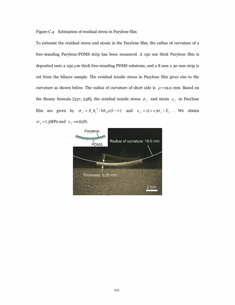
215

Figure C.4 Estimation of residual stress in Parylene film

To estimate the residual stress and strain in the Parylene film, the radius of curvature of a

free-standing Parylene/PDMS strip has been measured. A 150 nm thick Parylene film is

deposited onto a 250 mm thick free-standing PDMS substrate, and a 8 mm x 30 mm strip is

cut from the bilayer sample. The residual tensile stress in Parylene film gives rise to the

curvature as shown below. The radius of curvature of short side is =19.0 mm. Based on

the Stoney formula [237, 238], the residual tensile stress f and strain fe in Parylene

film are given by )1(6/2 -= fssf hhE and fff E/)1( e += . We obtain

f =7.3MPa and fe =0.63%.