Mechanical Characteristic Analysis of Buried Drainage ...
36
Prime Archives in Engineering 1 www.videleaf.com Book Chapter Mechanical Characteristic Analysis of Buried Drainage Pipes after Polymer Grouting Trenchless Rehabilitation Ren Wang 1,2,3 *, Jian-guo Xu 1,2,3 and Zhi-hao Chen 1,2,3 1 School of Water Conservancy Sci. & Eng. Institute of Underground Engineering, Zhengzhou University, China 2 National Local Joint Engineering Laboratory of Major Infrastructure Testing and Rehabilitation Technology, China 3 Collaborative Innovation Center of Water Conservancy and Transportation Infrastructure Safety, China *Corresponding Author: Ren Wang, School of Water Conservancy Sci. & Eng. Institute of Underground Engineering, Zhengzhou University, Zhengzhou 450001, China Published June 09, 2021 This Book Chapter is a republication of an article published by Ren Wang, et al. at Advances in Civil Engineering in February 2021. (Jian-guo Xu, Zhi-hao Chen, Ren Wang. Mechanical Characteristic Analysis of Buried Drainage Pipes after Polymer Grouting Trenchless Rehabilitation. Advances in Civil Engineering. Volume 2021, Article ID 6679412, 14 pages. https://doi.org/10.1155/2021/6679412) How to cite this book chapter: Ren Wang, Jian-guo Xu, Zhi- hao Chen. Mechanical Characteristic Analysis of Buried Drainage Pipes after Polymer Grouting Trenchless Rehabilitation. In: Mohamed Ali Hajjaji, editor. Prime Archives in Engineering. Hyderabad, India: Vide Leaf. 2021. © The Author(s) 2021. This article is distributed under the terms of the Creative Commons Attribution 4.0 International License(http://creativecommons.org/licenses/by/4.0/), which
Transcript of Mechanical Characteristic Analysis of Buried Drainage ...

Prime Archives in Engineering
1 www.videleaf.com
Book Chapter
Mechanical Characteristic Analysis of
Buried Drainage Pipes after Polymer
Grouting Trenchless Rehabilitation Ren Wang
1,2,3*, Jian-guo Xu
1,2,3 and Zhi-hao Chen
1,2,3
1School of Water Conservancy Sci. & Eng. Institute of
Underground Engineering, Zhengzhou University, China 2National Local Joint Engineering Laboratory of Major
Infrastructure Testing and Rehabilitation Technology, China 3Collaborative Innovation Center of Water Conservancy and
Transportation Infrastructure Safety, China
*Corresponding Author: Ren Wang, School of Water Conservancy Sci. & Eng. Institute of Underground Engineering,
Zhengzhou University, Zhengzhou 450001, China
Published June 09, 2021
This Book Chapter is a republication of an article published by
Ren Wang, et al. at Advances in Civil Engineering in February 2021. (Jian-guo Xu, Zhi-hao Chen, Ren Wang. Mechanical
Characteristic Analysis of Buried Drainage Pipes after Polymer
Grouting Trenchless Rehabilitation. Advances in Civil Engineering. Volume 2021, Article ID 6679412, 14 pages.
https://doi.org/10.1155/2021/6679412)
How to cite this book chapter: Ren Wang, Jian-guo Xu, Zhi-hao Chen. Mechanical Characteristic Analysis of Buried
Drainage Pipes after Polymer Grouting Trenchless
Rehabilitation. In: Mohamed Ali Hajjaji, editor. Prime Archives in Engineering. Hyderabad, India: Vide Leaf. 2021.
© The Author(s) 2021. This article is distributed under the terms
of the Creative Commons Attribution 4.0 International License(http://creativecommons.org/licenses/by/4.0/), which
Prime Archives in Engineering
2 www.videleaf.com
permits unrestricted use, distribution, and reproduction in any
medium, provided the original work is properly cited.
Data Availability: The data and code used in this study cannot
be shared at this time as the data also form a part of an ongoing
study.
Conflicts of Interest: The authors declare that they have no
conflicts of interest.
Acknowledgements: For financial support of this work we
gratefully acknowledge and thank the National Key R&D Program of China (2016YFC0401608), the National Natural
Science Foundation of China (No.52079128), the Scientific and
Technological Research Program of Henan province
(No.182102210013, 212102310289), and the Program for Innovative Research Team (in Science and Technology) in
University of Henan Province (No. 18IRTSTHN007). We also
acknowledge Top Edit LLC for the linguistic.
Abstract The application of Polymer grouting in underground pipeline rehabilitation is increasing gradually. The leakage and
subsidence of buried pipelines could be repaired by polymer
grouting technology. In order to analysis the calculation theory
of the pipeline repairing process, the Winkler model and the Vlazov model of the pipe-soil-polymer interaction based on the
elastoplastic theory is established, the calculation formulas of the
pipe-soil interaction under polymer grouting is derived and the MATLAB calculation program based on the transfer matrix
method is compiled. Then the calculated values are compared
with the pipeline experimental values, and the influence of
different factors on the internal force and deformation of the polymer-repaired pipeline under different work conditions is
discussed. The results show that the values and trends of the pipe
deformation and circumferential bending moment calculated by the models are consistent with the experimental results, and the
results obtained by the Vlazov model are closer to the
experimental values. In addition, the void at the bottom of the
Prime Archives in Engineering
3 www.videleaf.com
pipeline has a large impact on the mechanical properties of the
pipeline. However, polymer grouting can repair disengaged pipelines effectively and restore their mechanical properties. The
proposed methods and calculation results are valuable for
pipeline polymer repairing analysis and pipeline void repairing
design.
Introduction
The urban drainage network used for discharging urban foul water and rainwater is very important for modern cities.
However, most of the municipal drainage pipelines in China
were established before the 1980s. As the service life is
approaching, the pipelines are seriously aging, and they often have accidents such as disengagement, subsidence, corrosion and
leakage. These pipelines cannot work properly, which leads to
undesirable consequences, such as ground collapse and groundwater contamination [1]. The traditional way of repairing
drainage pipelines is mainly overall excavation and then
performing partial repairing or replacing the pipes. This method is expensive and has a serious impact on urban roads and
surrounding residents. Polymer grouting technology is an
effective trenchless rehabilitation technology for pipelines. It
uses a self-expanding anhydrous reactive polymer material that expands and solidifies rapidly after reaction. The polymer
grouting material is injected into the leaking area of the pipeline
to fill the void outside the pipe and lift the settlement pipe (see Figures 1 and 2). At present, the technology has successfully
reinforced and repaired various underground pipelines [2, 3].

Prime Archives in Engineering
4 www.videleaf.com
Figure 1: Polymer grouting fills the void outside the pipe.
Figure 2: Polymer grouting lifts the settlement pipe.
For the mechanical properties of polymer-repaired pipelines,
researchers often use finite element analysis software for
simulation or experimental exploration. But the research on the pipe calculation theory and methods after pipeline repair is not
enough. For example, Xu [4] used ABAQUS to simulate and
calculate the stress of polymer-repaired pipelines. The results showed that the maximum tensile and compression stress of the
pipes and the maximum vertical and horizontal displacements of
the pipes decreased significantly after polymer grouting. Li [5]
conducted a finite element analysis on the mechanical properties of repaired pipelines under vehicle loads, and the results showed
that the stress and deformation of the disengaged pipes repaired
by polymer restored to normal levels. Wang [6] conducted the field full-scale test was carried out for corrosion pipes with three
different pipe bedding states under different vehicle axle loads,

Prime Archives in Engineering
5 www.videleaf.com
then according to the field test, the refined three-dimensional
finite element models of corroded drainage pipes with dense, void and polymer repaired pipe beddings were established,
respectively, and the reliability of the test results was verified.
Zhang [7] used finite element analysis software to analyse the
effect of expansion and diffusion of polymer on pipe stress and strain, and the effect of polymer grouting repair on pipe stress
and displacement. By comparing the simulation values with the
experimental values, that can be matched the trends to prove the correctness and rationality of the numerical simulation values.
Wang [8] conducted a full-scale experiment on polymer-repaired
pipelines under impact loads and vehicle loads. The results showed that polymer grouting can effectively repair the void
pipeline and even restore its mechanical properties to normal
levels.
The buried pipes will deform because of overlaying soil and
ground loads. Then, the left and right sidewalls of the pipe will
squeeze the soil, which will cause the elastic resistance of soil to the pipeline and restrict pipe deformation and compensate for
pipe rigidity. Therefore, when we study the calculation and
analysis methods of buried pipes, the medium around the pipeline must be taken as a part of the pipe, and the pipe-soil
interaction must be considered. Many research results have been
done in this area. For example, Kjartanson [9] took the pipe as a
series of beam elements, and took the backfill soil around the pipe as a nonlinear material. Base on this, a finite element
analysis method for the pipe-soil interaction of buried pipes was
proposed. Lee [10] used finite element models to reflect the soil characteristics, backfill and in-situ conditions, and selected soil
models to measure the deflection of buried prestressed concrete
cylinder pipes. Base on this and considering the pipe-soil
interaction, a horizontal deflection equation of the underground pipeline was proposed. Jung [11] used the Mohr-Coulomb (MC)
yield surface for peak strength to constrain soil deformation
under strain and maximum uplift conditions, and the finite element model of pipe-soil interaction in granular soil is
established. Burkov [12] presents the model and analysis of the
stress-strain state of the soil-pipe interaction system, then analyzes the stress-strain state of the pipeline using the ANSYS.
Prime Archives in Engineering
6 www.videleaf.com
The calculation results show that the stress-strain state of the
pipeline depends on the depth of its location. Ke [13] used the Pasternak model to simulate the pipe-soil interaction and
calculated the vertical displacement of the soil which caused by
building a shield tunnel under the pipeline. The results showed
the vertical displacement of the pipeline by 15.3% due to the shear force in the soil. Based on the Winkler foundation beam
theory, Wang and Yao [14] gave the pipe-soil interaction model
of buried steel pipes and the calculation formulas of the deflection and internal force of buried steel pipes. According to
the measured results of buried pipeline stress characteristics, Liu
and Yang [15] established a pipe-soil interaction analysis combination model and presented a method of determining the
model parameters. The literature mostly focuses on the pipe-soil
interaction, but for the polymer-repaired pipeline, the pipe-soil-
polymer interaction should be considered. Therefore, a Winkler model and a Vlazov model considering the pipe-soil-polymer
interaction are proposed based on the elastoplastic theory. Using
the transfer matrix method, the MATLAB calculation program is compiled. By comparing the stress and deformation
characteristics before and after polymer grouting repairing for
underground pipeline to the experimental values, the accuracy and rationality of the Winkler model and Vlazov model are
discussed. Finally, the Vlazov model is used to calculate the
stress and deformation characteristics of the pipeline after
polymer grouting repairing.
Model of Pipe-Soil-Polymer Interaction
Analysis Winkler Model of Pipe-Soil-Polymer Interaction Winker proposes the idealized model of soil media. It assumes
that the displacement at any point on the soil surface medium is
proportional to the stress acting on that point, and is independent of the stress acting on other points [16]. The equation is as
follows:
),(),( yxkyxq (1)
Prime Archives in Engineering
7 www.videleaf.com
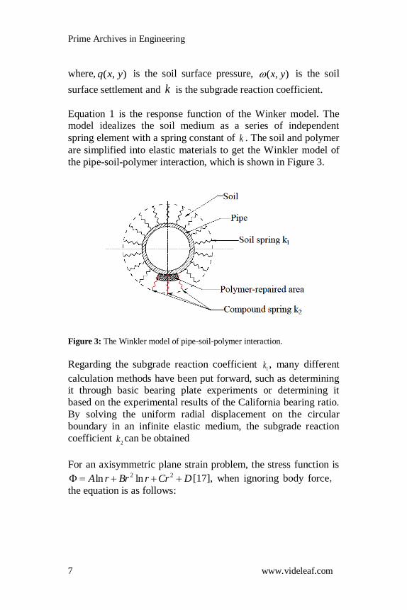
where, ),( yxq is the soil surface pressure, ),( yx is the soil
surface settlement and k is the subgrade reaction coefficient.
Equation 1 is the response function of the Winker model. The model idealizes the soil medium as a series of independent
spring element with a spring constant of k . The soil and polymer
are simplified into elastic materials to get the Winkler model of
the pipe-soil-polymer interaction, which is shown in Figure 3.
Figure 3: The Winkler model of pipe-soil-polymer interaction.
Regarding the subgrade reaction coefficient 1k , many different
calculation methods have been put forward, such as determining it through basic bearing plate experiments or determining it
based on the experimental results of the California bearing ratio.
By solving the uniform radial displacement on the circular
boundary in an infinite elastic medium, the subgrade reaction
coefficient 2k can be obtained
For an axisymmetric plane strain problem, the stress function is
DCrrBrrA 22 lnln [17], when ignoring body force,the equation is as follows:
Prime Archives in Engineering
8 www.videleaf.com
0
2)ln23(
2)ln21(1
22
2
2
r
r
CrBr
A
r
CrBr
A
rr
(2)
In Equation 2, is the stress coefficient, A , B ,C and D are the
coefficients, r is the radius. r and
are the radial stress and
tangential stress, respectively.
By the displacement single value property,the coefficient
=0B ,and at infinity from the origin, the stresses
0 r from the Saint Venant's Principle, thus =0C .
Substitute =0B and =0C into Equation 2 to simplify and the
equation is as follows:
22
2
2
1
r
A
r
r
A
rrr
(3)
Substitute Equation 3 into Hooke's plane strain law, the equation
can be described as
2
s
2
21
)1()(
1
)1()(
1
rE
A
E
rE
A
E
s
ssrr
g
g
gr
g
r
(4)
where 1r and
2r are the strain of the polymer layer and soil
layer, respectively. gE and
g are the elastic modulus and
Poisson ratio of polymer, respectively. sE and
s are the elastic
modulus and Poisson ratio of soil, respectively. The uniform
Prime Archives in Engineering
9 www.videleaf.com
radial displacement on the circular boundary is calculated by the
following equation:
drdruDR
r
DR
R
r
21 (5)
where D is the polymer layer thickness.
Substitute Equation 4 into the Equation 5 to get the radial
displacement:
RE
A
EEDR
Au
g
ggs)1(11
gs
(6)
With the elastic parameters k defined in the Winker model and
Equations. 3 and 6, the subgrade reaction coefficient of the
polymer layer is:
g
g
g
g
s
s
r
E
R
EEDR
Ruk
)1(11
1
22
(7)
Vlazov Model of Pipe-Soil-Polymer Interaction Because the Winkler model has inherent defects in describing
the continuity of natural soil, it is suitable for the case where the
foundation soil (compression layer) is thin. The more the compression layer is thick, the greater error will become. To
make up for the defects of the Winkler model, researchers get a
new two-parameter model by introducing constraints in the
elastic continuous medium model or simplifying certain assumptions of displacement distribution and stress [16]. The
Vlazov model is one of them and it is based on variational
calculus. The model formula by introducing some displacement constraints to simplify the basic equations of the isotropy linear
Prime Archives in Engineering
10 www.videleaf.com
elasticity continuous medium model and the equation is as
follows:
),(),(),( 2 yxTyxKyxq (8)
where ),( yxq is the soil surface pressure, ),( yx is the soil
surface settlement, 2 is the Laplace operator, K is the
measure of soil deformation under compression stress, T is the
measure of soil unit transitivity.
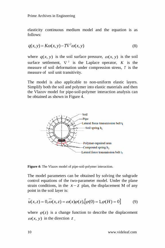
The model is also applicable to non-uniform elastic layers.
Simplify both the soil and polymer into elastic materials and then
the Vlazov model for pipe-soil-polymer interaction analysis can be obtained as shown in Figure 4.
Figure 4: The Vlazov model of pipe-soil-polymer interaction.
The model parameters can be obtained by solving the subgrade
control equations of the two-parameter model. Under the plane
strain conditions, in the zx plan, the displacement M of any
point in the soil layer is:
0)(,1)0(),()(),(,0),( Hzxzxzxu (9)
where )(z is a change function to describe the displacement
),( yx in the direction z .
Prime Archives in Engineering
11 www.videleaf.com
Based on the relationship between the stress and strain under the
plane strain conditions, the equation is as follows:
)()()1(2
)()(1
)()()1(2
)()(1
2
22
2
2
22
1
11
2
1
11
zxE
zxE
zxE
zxE
xz
z
xz
z
(10)
where )1/(2
1 ggEE , )1/(1 gg )1/(2
2 ssEE ,
)1/(2 ss , gE and g are the elastic modulus and the
Poisson ratio of polymer, respectively, sE and s are the elastic
modulus and the Poisson ratio of soil, respectively.
According to Lagrange virtual work principle, the virtual
displacement is 0u , )(z . The virtual work done
by the external force is:
dxdzzx
bdxdxzx
bdxxbqU
H
H
xz
H
xze
)()()0()(
1
1
2
0
1
(11)
The virtual work done by the internal force is:
dxdzzbdxdzzbU
H
H
z
H
zi )()(
1
1
2
0
1 (12)
Substituting Equation 10 into
0 ie UU ,the equation can
be described as:
2
2 )(2)()(
dx
xdTxKxq
(13)
where
Prime Archives in Engineering
12 www.videleaf.com
H
H
H
dzzE
dzzE
K
1
1
2
2
2
2
0
2
2
1
1 )]([1
)]([1
,
dzzE
dzzE
T
H
H
H
)1(4
)1(4
1
1
2
2
2
0
2
1
1
(
)(
)
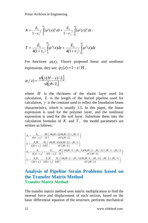
For functions )(z , Vlazov proposed linear and nonlinear
expressions, they are:
Hzz /1)(1 ,
Lhsh
LzHshz
/
/)()2
( .
where H is the thickness of the elastic layer used for
calculation, L is the length of the buried pipeline used for
calculation, is the constant used to reflect the foundation beam
characteristics, which is usually 1.5. In this paper, the linear
expression is used for the polymer layer, and the nonlinear expression is used for the soil layer. Substitute them into the
calculation formulas of K and T , the model parameters are
written as follows:
)/(
//)//()//(
2
3
)1(12)1(12
)/(
//)//()//(
2)1()1(
)/(
/)/()/(
2
3
)1(12
)/(
/)/()/(
2)1(
2
111
2
2
1
112
2
111
2
2
2
2
11
12
2
2
21
22
2
21
LHsh
LHLHLHLHchLHLHsh
H
L
v
HE
v
HET
LHsh
LHLHLHLHchLHLHsh
L
H
vH
E
vH
EK
LHsh
LHLHchLHsh
H
L
v
HET
LHsh
LHLHchLHsh
L
H
vH
EK
Analysis of Pipeline Strain Problems based on
the Transfer Matrix Method Transfer Matrix Method
The transfer matrix method uses matrix multiplication to find the internal force and displacement of each section, based on the
basic differential equation of the structure, performs mechanical

Prime Archives in Engineering
13 www.videleaf.com
analysis of the structure [18]. Because of using simple matrix
multiplication, it is suitable for calculations using computer programming. Compared with the finite element method, the
transfer matrix method prevents the overall stiffness matrix from
being too large,which makes it difficult to solve large linear
systems [19]. At the same time, it does not need to select a suitable soil constitutive model and set up contact elements,
which will make calculation simply. Therefore, this method has
simple calculations. The calculation process can be expressed by the following formula:
0121 SUUUUS iii (14)
where 0S is the initial situation vector, iS is the end situation
vector, 1U , 2U iU , 1iU is the transfer matrix of each part.
Description of the Pipeline Calculation Model Due to the existence of the pipe joints, the pipeline structure is
discontinuous. It is difficult to theoretically consider the
interaction of each pipe section and joints. In view of the problems studied in this article, it is necessary and feasible to
simplify the model by ignoring some secondary factors. At the
non-joints, we simulate the pipeline as a horizontally homogeneous circular ring and a longitudinal continuous
cylinder. Then we assume that the length of pipeline is long
enough and the external load is evenly distributed along the axial
direction of the pipe. Therefore, the calculation of pipeline stress and deformation can be regarded as a plane strain problem. At
the joints, according to the longitudinal equivalent continuity
model proposed by Shiba Yukio [20-21], the connection effect of joints and pipe section can be considered by equivalent stiffness,
then calculated according to the above method. In the paper, to
simplify the calculation, we only consider the pipe at the non-joints. The load acting on the pipeline is considered to be
symmetrical, so only half of the pipeline is calculated and
analyzed. As shown in Figure 5, a unit length pipeline is chosen.
the wall thickness and radius of the pipeline are t and R ,
respectively. Half of the pipeline is divided into n units. At the
Prime Archives in Engineering
14 www.videleaf.com
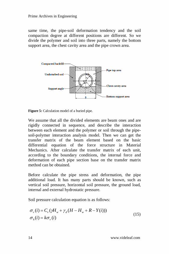
same time, the pipe-soil deformation tendency and the soil
compaction degree at different positions are different. So we divide the polymer and soil into three parts, namely the bottom
support area, the chest cavity area and the pipe crown area.
Figure 5: Calculation model of a buried pipe.
We assume that all the divided elements are beam ones and are rigidly connected in sequence, and describe the interaction
between each element and the polymer or soil through the pipe-
soil-polymer interaction analysis model. Then we can get the transfer matrix of the beam element based on the basic
differential equation of the force structure in Material
Mechanics. After calculate the transfer matrix of each unit,
according to the boundary conditions, the internal force and deformation of each pipe section base on the transfer matrix
method can be obtained.
Before calculate the pipe stress and deformation, the pipe
additional load. It has many parts should be known, such as
vertical soil pressure, horizontal soil pressure, the ground load, internal and external hydrostatic pressure.
Soil pressure calculation equation is as follows:
)()(
)))((()(
iki
iYRHHHCi
h
wdw
(15)
Prime Archives in Engineering
15 www.videleaf.com
Where: )(i and )(ih are vertical soil pressure and
horizontal soil pressure, H and wH are pipe depth and
groundwater level depth, and d are dry soil bulk density and
saturated soil bulk density, R is pipe radius, )(iY is Y
coordinate at node i , k is lateral pressure coefficient of soil
pressure. C is soil pressure concentration factor, in this paper,
which determined based on Liu's research results [22].
The ground load is the general term for all loads acting on the gr
ound. It mainly includes traffic load and building load, the pipe p
ressure caused by the ground load can be calculated according to the Bousinesq [17] formula. Hydrostatic pressure calculation equ
ation is as follows:
))((
))((
iYR
iYRHH
wwi
wwwo
(16)
Where, wo and wi are external and internal hydrostatic
pressure, w is water bulk density.
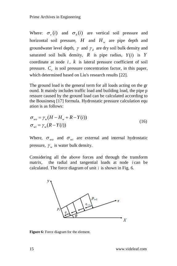
Considering all the above forces and through the transform
matrix, the radial and tangential loads at node i can be
calculated. The force diagram of unit i is shown in Fig. 6.
Figure 6: Force diagram for the element.

Prime Archives in Engineering
16 www.videleaf.com
In Figure 6, ip and iq are the radial and tangential loads at node
i , respectively. 1ip and 1iq are the radial and tangential loads
at node 1i , respectively. l is the length of unit i . is the
angle between unit i and X axis in the overall coordinate
system.
Under the action of additional force, assume that the tangential
displacement at node i of unit i is iu , the radial displacement is
iv , the rotation angle is i , the bending moment is iM , the
axial force is iN , and the shear force is iT . The interaction
between unit i and the polymer or soil is described by the pipe-
soil-polymer interaction analysis Vlazov model. Then in the local coordinate, according to equilibrium conditions and
physical equations, the formulas for calculation are as follows:
dx
dv
EI
M
dx
vd
ES
N
dx
du
Tdx
dM
l
xq
l
xq
dx
dN
l
xp
l
xp
dx
xydTyK
dx
dT
ii
ii
2
2
1
12
2
1
1)(
2
(17)
where, K and T are Vlazov model parameters, E is pipe
elastic modulus, S is inertia moment of pipe section, I is cross-
sectional area of pipe element.
By solving the above Equation 17, and with the boundary
conditions: iuu , i , i , iMM , iNN , iTT

Prime Archives in Engineering
17 www.videleaf.com
when 0x , and 1 iuu , 1 i , 1 i , 1 iMM ,
1 iNN , 1 iTT when lx , the formula for calculation is
as follows:
iiii SUS ][ 1,1 (18)
where 1,,,,, ,iiiiiii TNMuS is the matrix of the
internal force and displacement at node i , ][ 1, iiU is the transfer
matrix of 77 , 1 1 1 1 1 1 1, , , , , 1i i i i i i iS u M N T , is the
matrix of the internal force and displacement at node 1i .
The transfer matrix, internal force and displacement matrix are all belong to the local coordinate. When calculating the internal
force and displacement of each element, the transfer matrix
needs to be converted into global coordinates. Through the
coordinate transform matrix R, we can transform Equation 18 into global coordinates as shown in the following equation:
iiii SUS ][ 1,1 (19)
where 1
1,1, ][][
RURU iiii is the transfer matrix of unit i ,
iS and 1iS are the matrices of the internal forces and
displacements at node i and node 1i in the global coordinate,
respectively. R is the coordinate transform matrix of unit i .
With the transfer matrix of each unit, the following equation by
substituting it into Equation 14 can be written as follwes:
12,13,2,11, ]][[]][[ SUUUUS nnnnn (20)
where 1S and nS are the matrices of the internal forces and
displacements at node 1 and node n .

Prime Archives in Engineering
18 www.videleaf.com
Since the load is symmetrical, according to the constraints of
boundary conditions, 1u = 1 = 1T =0, nu = n = nT =0 at node 1
and node n , 111 NM ,, and nnn NM ,, can be calculated
with Equation 20.
Then taking node 1 as a known quantity and substituting it into
Equation 21, the internal force and displacement of any node
can be calculated and the Equation is as follows:
12,13,2,11, ]][[]][[ SUUUUS iiiii (21)
After calculating the displacement of each node, the
corresponding contact pressure of each element can be determined. Combining the soil elastoplastic deformation law
and the pipe deformation, a part of the contact pressure is limited
to meet the plasticity conditions of the soil and the iterative calculation is used to meet all the boundary conditions and
deformation criteria.
Program Implementation
According to the above calculation process, MATLAB is used to compile the pipeline stress calculation program. The calculation
flowchart is as follows:

Prime Archives in Engineering
19 www.videleaf.com
Enter basic parameters: pipeline parameters, soil
parameters, external loads, etc
Calculate the load acting on
pipeline
Calculate pipe-soil-polymer
interaction model parameters
Calculate the transfer matrix of
each unit according to formula
Find internal force and displacement of the initial node
according to boundary conditions
Find internal force and displacement of each node one
by one according to treating initial point as a known
point
Whether the contact pressure of each
element meets soil elastic-plastic
deformation rule
Modify the contact pressure
to meet soil plastic condition
Output result: internal force and
displacement of each node
Recalculate the load acting
on pipeline
Y
N
Figure 7: Flow chart of the pipeline stress calculation program.
Experimental Description and Data Processing The experiments are carried out in a relatively open outdoor
area. A relatively flat place is selected. The experimental pits,
the length, width and depth of which are 8 m, 2.3 m and 2.3 m, respectively, are excavated using small equipment. Due to over-
excavation and soil disturbance at the bottom of the pit, the
undisturbed soil at the bottom is layered and compacted to a
depth of 0.36 m below the bottom of the pit before laying the pipeline. Three complete tube sections and two half-tube
sections are selected, which are connected through bell and
spigot joints (rubber rings are used as seals to prevent leakage). The effective length is 8 m. After the pipe is in place, the trench
is backfilled with several layers of loose soil, and the thickness
of each layer is about 0.2 m. The soil is then compacted by a small rammer. Then perform a normal, empty, polymer repair

Prime Archives in Engineering
20 www.videleaf.com
condition test on the same pipeline. At void area, when the
pipeline has no leakage and the sinking pipe section is raised to the design elevation after polymer repair, we think buried
drainage pipes can work properly.
The test pipe failure criteria based on GB/T 50332 (2002) [23], each pipe segment having a nominal inner diameter of 700 mm,
wall thickness of 70 mm, and an effective length of 2000 mm.
The strength of the concrete used for pipe making was C30, and the standard value of its compressive strength was 30 MPa. The
internal and external strains of the pipe under load are measured
by attaching strain gauges to the inner and outer walls of the pipe. During the tests, the mechanical responses of the pipe to
the loads are small, far from reaching the ultimate strength of the
material. Therefore, the pipeline can be considered to be still in
its elastic phase during the tests. The performance parameters of the pipeline, soil and polymer involved in the experiments are
shown in Table 1. The experimental pipeline cross-section and
the field experimental diagram are shown in Figure 8.
Table 1: Performance parameters of the pipeline, soil and polymer used in the experiment.
Material Density
/
Kg·m-3
Elastic modulus
E / MPa
Poisson ratio
Cohesive force C /
kPa
Internal friction angle
/
Dilatancy
angle /
Pipe 2400 30000 0.3 — — —
Soil 1980 60 0.3 40 30 0
Polymer 240 20 0.2 — — —

Prime Archives in Engineering
21 www.videleaf.com
Figure 8: Sectional view of the experimental pipeline and the pictures of the field experiment: (a) plan view, (b) north-south section view (through the cross-section of the pipeline), (c) east-west section view (unit: meter), (d) and (e) are pictures of the field experiment.
The experimental data should be processed to better compare the
experimental value with the calculation result of the model. The relationship between the pipe bending moment and the strain of
the inner and outer pipe walls is described as follows [24]:
hEIM outin
(22)
where M is the pipe bending moment, E is the pipe elastic
modulus, I is the moment of inertia, in and out are the
internal and external pipe strain, respectively and h is the pipe
thickness.
In the pipeline design, the ability of a pipeline to withstand
external loads is defined by the pipe stiffness, which is related to
the geometry and material of pipes. At the same time, in ASTM D 2412-11[25], the pipe stiffness is also defined as: the ratio of
the load that causes a certain percentage of pipe deformation
(5%) to the pipe inner diameter deformation along the load direction. Therefore, the pipe radial deformation can be
calculated by

Prime Archives in Engineering
22 www.videleaf.com
PS
Fy (23)
where y is the pipe radial deformation, F is the pipe radial
stress and PS is the pipe stiffness.
Comparing Model Calculation Results with
Experimental Results According to the experiment, the static load acting pipe section
is taken as the calculation pipeline, and different pipe-soil-
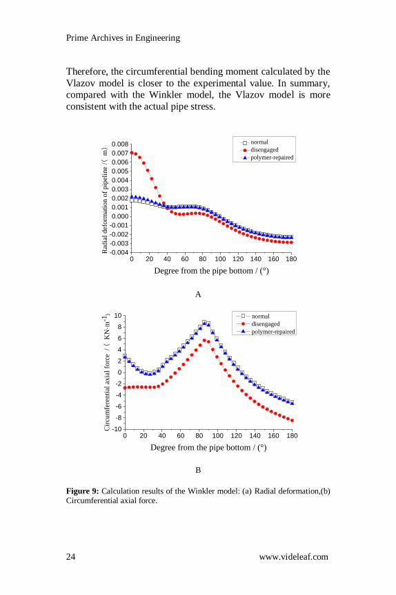
polymer interaction models are used for simulation. The calculation results are shown in Figure 9 and Figure 10. Figure 9
presents the radial deformation and circumferential axial force
calculated by the Winkler model under normal, disengaged and
polymer-repaired conditions. Figure 10 presents the results calculated by the Vlazov model. It can be seen from Figure 9 and
Figure 10 that the radial deformation of the pipe after polymer
repair is slightly larger than the normal value, and the circumferential axial force is basically the same as the normal
value. The maximum radial deformation difference under normal
and polymer-repaired appears at bottom of the pipe and it is 0.4 mm in Figure 9a and 1 mm in Figure 10a. The deformation and
mechanical properties of pipes after polymer grouting can be
restored to normal levels. Under disengaged conditions, the
radial deformation at the bottom and the circumferential axial force at the crown will increase significantly. Compared with the
normal situation, the radial deformation at the bottom increases
by 3.9 times (see Figure 9a) and 5.3 times (see Figure 10a), and the circumferential axial force at the crown increases by 1.6
times (see Figure 9b) and 2.0 times (see Figure 10b),
respectively. It shows that the bottom void has a great influence
on the mechanical properties of the pipe. At the same time, as shown in Figure 9 and Figure 10, the radial deformation of the
entire pipe will increase in a disengaged state, because the lack
of soil at the bottom can change the pipe constraints. Therefore, the pipe deformation will increase when a load is applied.

Prime Archives in Engineering
23 www.videleaf.com
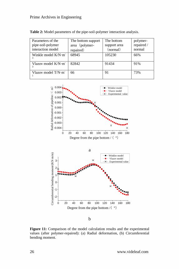
Figure 11 presents the comparison of the radial deformation and
the circumferential bending moment calculated by different analysis models with the experimental values. Table 2 lists the
parameters of the pipe-soil-polymer interaction analysis model
under normal and polymer repair conditions. Table 3 lists the
sample point data of the experiment. As shown in Table 2, the coefficient of the subgrade reaction after polymer repair
calculated by the Winkler model is 66% of the normal value, and
that calculated by the Vlazov model is 91% of the normal value. It shows that the results calculated by the Vlazov model are
closer to normal. As shown in Figure 11, the radial deformation
and the circumferential bending moment calculated by the models are basically consistent with the experimental values, and
the maximum radial deformation difference is 2 mm compared
with the experimental values. The small error indicates that the
calculation method is reliable. The calculation result of the Vlazov model is obviously larger than that of the Winkler model.
This is because the Vlazov model increases the soil lateral force
transmission so that the load transferability of the soil medium is more reasonable than that of the Winkler model. But compared
with the experimental value, the model calculation will have a
certain error. This is because in the calculation, we assume that the soil is an elastic body, but the soil is not completely elastic.
On the other hand, we assume that the polymer repair area is the
same length as the pipeline in the longitudinal direction, but the
length of the polymer repair area will be relatively short in the engineering practical projects.
As shown in Figure 11a, the radial deformation calculated by the Vlazov model is close to the experimental value. Except for the
pipe crown, the calculation error is between 2% and 25%. At the
45° haunch, the model calculation result is closest to the
experimental value. The calculation error of the Winkler model is relatively large, which is between 9% and 55%. As shown in
Figure 11b, regarding the calculation of the circumferential
bending moment, the errors between the calculation results of the Winkler model and experimental values are 35%, 21% and 12%
at the bottom, spring line and crown, respectively. The errors
between the calculation results of the Vlazov model and the experimental values are 18%, 16% and 11%, respectively.
Prime Archives in Engineering
24 www.videleaf.com
Therefore, the circumferential bending moment calculated by the
Vlazov model is closer to the experimental value. In summary, compared with the Winkler model, the Vlazov model is more
consistent with the actual pipe stress.
0 20 40 60 80 100 120 140 160 180-0.004
-0.003
-0.002
-0.001
0.000
0.001
0.002
0.003
0.004
0.005
0.006
0.007
0.008
Rad
ial
def
orm
atio
n o
f pip
elin
e /(
m)
Degree from the pipe bottom / (°)
normal
disengaged
polymer-repaired
A
0 20 40 60 80 100 120 140 160 180-10
-8
-6
-4
-2
0
2
4
6
8
10
Cir
cum
fere
nti
al a
xia
l fo
rce
/ (
KN
·m-1
)
Degree from the pipe bottom / (°)
normal
disengaged
polymer-repaired
B
Figure 9: Calculation results of the Winkler model: (a) Radial deformation,(b) Circumferential axial force.

Prime Archives in Engineering
25 www.videleaf.com
0 20 40 60 80 100 120 140 160 180-0.008
-0.006
-0.004
-0.002
0.000
0.002
0.004
0.006
0.008
0.010
0.012
0.014
0.016
Rad
ial
def
orm
atio
n o
f pip
elin
e /(
m)
Degree from the pipe bottom / (°)
normal
disengaged
polymer-repaired
a
0 20 40 60 80 100 120 140 160 180-14
-12
-10
-8
-6
-4
-2
0
2
4
6
8
10
Cir
cum
fere
nti
al a
xia
l fo
rce
/ (K
N·m
-1)
Degree from the pipe bottom / (°)
normal
disengeged
polymer-repaired
B
Figure 10: Calculation results of the Vlazov model: (a) Radial deformation,(b)
Circumferential axial force.
Prime Archives in Engineering
26 www.videleaf.com
Table 2: Model parameters of the pipe-soil-polymer interaction analysis.
Parameters of the pipe-soil-polymer
interaction model
The bottom support
area(polymer-
repaired)
The bottom support area
(normal)
polymer-repaired /
normal
Winkle model K/N·m-
3 68945 105230 66%
Vlazov model K/N·m-
3 82842 91434 91%
Vlazov model T/N·m-
1
66 91 73%
0 20 40 60 80 100 120 140 160 180
-0.004
-0.003
-0.002
-0.001
0.000
0.001
0.002
0.003
0.004
Rad
ial
def
orm
atio
n o
f p
ipel
ine
/ (
m)
Degree from the pipe bottom / ( °)
Winkler model
Vlazov model
Experimental value
a
0 20 40 60 80 100 120 140 160 180
-2
-1
0
1
2
3
Cir
cum
fere
nti
al b
end
ing
mo
men
t/(K
N·m
/m)
Degree from the pipe bottom /( °)
Winkler model
Vlazov model
Experimental value
b
Figure 11: Comparison of the model calculation results and the experimental values (after polymer-repaired): (a) Radial deformation, (b) Circumferential bending moment.

Prime Archives in Engineering
27 www.videleaf.com
Table 3: The sample point data of the experiment
Sample point(degree from the pipe bottom) /°
Internal pipe strain/
External pipe strain/
Pipe radial stress/ kPa
0 4.868 1.503 63.201
45 5.174 3.842 76.324
90 5.203 0.701 50.504
135 -6.012 -4.507 -100.761
180 -6.678 -3.958 -135.723
Influence of Different Factors on the Internal
Force and Deformation of Pipelines after
Polymer Repair
The internal force and deformation of a buried pipeline are
affected by many factors, such as the depth, diameter and
material of the pipeline, the ground load and the nature of surrounding filler. The pipe-soil-polymer interaction simulated
by the Vlazov model is more in line with the actual situation. So
the Vlazov model is used to calculate the pipeline after repaired with polymer grouting under different working conditions to
explore the influence of different factors on the internal force
and deformation after repair.
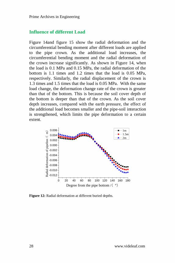
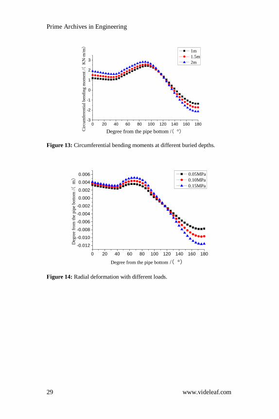
Influence of Soil Cover Depth Figure 12 and figure 13 show the radial deformation and the
circumferential bending moment after polymer-repair when the
soil cover depth is 1 m, 1.5 m and 2 m, respectively. At different cover depths, the radial deformation and bending moment
change trends are consistent. As the cover depth increases, its
value will increase significantly. This is because the overburden
pressure of the pipe will increase as the cover depth increases, which will result in increased stress and deformation. In Figure
12, as different coordinate systems are used, although the bottom
deformation is positive and the crown is negative, both are downward and the deformation at the crown is greater than that
at the bottom. As shown in Figure 13, the maximum value of the
circumferential bending moment appears at the spring line.
Prime Archives in Engineering
28 www.videleaf.com
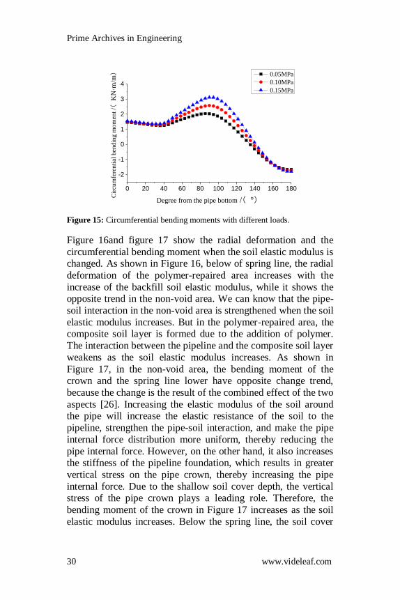
Influence of different Load
Figure 14and figure 15 show the radial deformation and the
circumferential bending moment after different loads are applied
to the pipe crown. As the additional load increases, the circumferential bending moment and the radial deformation of
the crown increase significantly. As shown in Figure 14, when
the load is 0.1 MPa and 0.15 MPa, the radial deformation of the bottom is 1.1 times and 1.2 times that the load is 0.05 MPa,
respectively. Similarly, the radial displacement of the crown is
1.3 times and 1.5 times that the load is 0.05 MPa. With the same
load change, the deformation change rate of the crown is greater than that of the bottom. This is because the soil cover depth of
the bottom is deeper than that of the crown. As the soil cover
depth increases, compared with the earth pressure, the effect of the additional load becomes smaller and the pipe-soil interaction
is strengthened, which limits the pipe deformation to a certain
extent.
0 20 40 60 80 100 120 140 160 180
-0.012
-0.010
-0.008
-0.006
-0.004
-0.002
0.000
0.002
0.004
0.006
Rad
ial
def
orm
atio
n o
f p
ipel
ine
/(m)
Degree from the pipe bottom /( °)
1m
1.5m
2m
Figure 12: Radial deformation at different buried depths.
Prime Archives in Engineering
29 www.videleaf.com
0 20 40 60 80 100 120 140 160 180-3
-2
-1
0
1
2
3
Cir
cum
fere
nti
al b
endin
g m
om
ent
/(K
N·m
/m)
Degree from the pipe bottom /( °)
1m
1.5m
2m
Figure 13: Circumferential bending moments at different buried depths.
0 20 40 60 80 100 120 140 160 180
-0.012
-0.010
-0.008
-0.006
-0.004
-0.002
0.000
0.002
0.004
0.006
Deg
ree
from
the
pip
e bott
om
/(
m)
Degree from the pipe bottom /( °)
0.05MPa
0.10MPa
0.15MPa
Figure 14: Radial deformation with different loads.
Prime Archives in Engineering
30 www.videleaf.com
0 20 40 60 80 100 120 140 160 180
-2
-1
0
1
2
3
4
Cir
cum
fere
nti
al b
end
ing
mo
men
t /(
KN
·m/m)
Degree from the pipe bottom /( °)
0.05MPa
0.10MPa
0.15MPa
Figure 15: Circumferential bending moments with different loads.
Figure 16and figure 17 show the radial deformation and the
circumferential bending moment when the soil elastic modulus is changed. As shown in Figure 16, below of spring line, the radial
deformation of the polymer-repaired area increases with the
increase of the backfill soil elastic modulus, while it shows the opposite trend in the non-void area. We can know that the pipe-
soil interaction in the non-void area is strengthened when the soil
elastic modulus increases. But in the polymer-repaired area, the composite soil layer is formed due to the addition of polymer.
The interaction between the pipeline and the composite soil layer
weakens as the soil elastic modulus increases. As shown in
Figure 17, in the non-void area, the bending moment of the crown and the spring line lower have opposite change trend,
because the change is the result of the combined effect of the two
aspects [26]. Increasing the elastic modulus of the soil around the pipe will increase the elastic resistance of the soil to the
pipeline, strengthen the pipe-soil interaction, and make the pipe
internal force distribution more uniform, thereby reducing the
pipe internal force. However, on the other hand, it also increases the stiffness of the pipeline foundation, which results in greater
vertical stress on the pipe crown, thereby increasing the pipe
internal force. Due to the shallow soil cover depth, the vertical stress of the pipe crown plays a leading role. Therefore, the
bending moment of the crown in Figure 17 increases as the soil
elastic modulus increases. Below the spring line, the soil cover

Prime Archives in Engineering
31 www.videleaf.com
depth is thick and the pipe-soil interaction plays a dominant role.
Therefore, the bending moment is reduced accordingly.
Influence of different Pipe Thickness Figure 18and figure19 show the radial deformation and the
circumferential bending moment when the pipe thickness is
changed. The circumferential bending moment increases as the thickness of the pipe wall increases, and the radial deformation
shows the opposite trend. This is because the wall thickness of
the pipelines with the same diameter is different, so the bending stiffness is also different. With the thickness increasing of the
pipe, the pipe section stiffness increased, resulting in the
reduction of the radial deformation. And the stiffness increasing
will also reduce the deformation coordination ability between the pipe and the soil and increase the vertical stress of the pipe
crown, thereby increasing the stress distribution around the pipe,
so the bending moment will also increase.
0 20 40 60 80 100 120 140 160 180
-0.012
-0.010
-0.008
-0.006
-0.004
-0.002
0.000
0.002
0.004
0.006
Rad
ial
def
orm
atio
n o
f p
ipel
ine
/(m)
Degree from the pipe bottom /( °)
40Mpa
60Mpa
80Mpa
Figure 16: Radial deformation at different soil elastic modulus

Prime Archives in Engineering
32 www.videleaf.com
0 20 40 60 80 100 120 140 160 180
-2
-1
0
1
2
3
Cir
cum
fere
nti
al b
endin
g m
om
ent /(
KN
·m/m)
Degree from the pipe bottom /( °)
40Mpa
60Mpa
80Mpa
Figure 17: Circumferential bending moments at different soil elastic modulus
0 20 40 60 80 100 120 140 160 180
-0.010
-0.008
-0.006
-0.004
-0.002
0.000
0.002
0.004
0.006
Rad
ial
def
orm
atio
n o
f p
ipel
ine
/(m)
Degree from the pipe bottom /( °)
12mm
24mm
36mm
Figure 18: Radial deformation with different pipe thickness
0 20 40 60 80 100 120 140 160 180
-4
-2
0
2
4
6
Cir
cum
fere
nti
al b
endin
g m
om
ent
/(K
N·m
/m)
Degree from the pipe bottom /( °)
12mm
24mm
36mm
Figure 19: Circumferential bending moments with different pipe thickness

Prime Archives in Engineering
33 www.videleaf.com
Conclusions In order to analyze the stress and deformation characteristics of the underground pipeline after polymer repair, the Winkler
model and the Vlazov model are be presented by considering the
pipe-soil-polymer interaction based on the elastoplastic theory
and the MATLAB calculation program is compiled based on the transfer matrix method. By comparing the stress and the
deformation characteristics of the underground pipeline before
and after polymer grouting repairing, and making use of experimental results, the accuracy and rationality of the Winkler
model and the Vlazov model are discussed. Finally, the Vlazov
model is chosen to study the pipe deformation characteristics after repair. The working conditions include the pipeline depth,
load concentration, backfill soil elastic modulus and pipeline
wall thickness, etc. The conclusions are drawn in the following.
The radial deformation and the circumferential bending
moment calculated by the Winkler model and the Vlazov
model considering the pipe-soil-polymer interaction are
consistent with experimental results, which verifies the accuracy and rationality of the models. The calculation
results of the Vlazov model are closer to the experimental
results.
The void has a great influence on the overall mechanical
properties of pipelines. The void area at the bottom
significantly increases the radial deformation and the axial
internal force of the pipeline. However, after the polymer
grouting repair, the radial deformation and the axial internal force are close to a normal pipeline, which indicates that the
polymer grouting can repair the pipeline effectively.
With the soil cover depth increases, the radial deformation
and bending moment increase significantly. This is because the overburden pressure of the pipeline will increase with the
soil cover depth, resulting in an increase of the stress and
deformation.
The radial deformation of the pipeline decreases as the
backfill soil elastic modulus increases. With the increase of
the backfill soil elastic modulus around the pipeline, the
pipe-soil interaction is also strengthened, which is beneficial
Prime Archives in Engineering
34 www.videleaf.com
to the development of the soil medium supporting effect. It is
beneficial to the stress of the entire pipe.
The circumferential bending moment increases as the
thickness of the pipe wall increases, while the trend of the
radial deformation is the opposite. An increase in the
thickness of the pipe wall increases the pipe section stiffness,
resulting in a reduction of the pipe radial deformation.
Polymer grouting is an effective trenchless repair technology
for pipelines. It uses a self-expanding anhydrous reactive
polymer material that expands and solidifies rapidly after
reaction. The polymer grouting material is injected into the leaking area of the pipeline to fill the void outside the pipe
and lift the settlement pipe. At present, the technology has
successfully reinforced and repaired various underground pipelines. This study provides a theoretical reference for the
design and construction of pipeline polymer repairs.
References 1. MB Lin. Health inspection and analysis of sewer system in
an area of Fuzhou city. China Water & Waste water. 2014;
30: 96-98. 2. M Shi, F Wang, J Luo. Compressive strength of polymer
grouting material at different temperatures. Journal of
Wuhan University of Technology-Materials Science Edition. 2010; 25: 962-965.
3. Y Tang, BQ Li, XN Xiao. Application of polymer grouting
technology for urban sewage pipeline rehabilitation. Water
Purification Technology. 2015; 34: 90-93. 4. JG Xu, HM Hu, YH Zhong. Numerical analysis on
underground pipe settlement and vacancy repairing with
polymer injection. Chinese Journal of Underground Space and Engineering. 2017; 13: 1165-1172.
5. B Li, HY Fang, FM Wang. Analysis of the mechanical
characteristics of disengaging drainage pipe before and after
polymer repairing. Journal of Zhengzhou University (Engineering Edition). 2019; 40: 62-66.
6. FM Wang, B Li, HY Fang. Experimental and numerical
study on polymer grouting repair of underground pipeline with void and corrosion diseases. Hazard Control in

Prime Archives in Engineering
35 www.videleaf.com
Tunnelling and Underground Engineering. 2019; 1: 1-8.
7. QQ Zhang. Numerical simulation of repairing by polymer grouting for drainage pipeline voids, MS Thesis, Zhengzhou
University. Zhengzhou, China. 2019.
8. Ren Wang, Fuming Wang, Jianguo Xu, Yanhui Zhong,
Shikun Li. Full-scale experimental study of the dynamic performance of buried drainage pipes under polymer
grouting trenchless rehabilitation. Ocean Engineering. 2019;
181: 121-133. 9. Kjartanson BH, Heilers GA, Lohnes RA, Klaiber FW. Soil-
structure interaction analysis of longitudinal uplift of
culverts. Journal of Geotechnical and Geoenvironmental Engineering. 1998; 124: 128-139.
10. Y Lee, MQ Feng, ET Lee. Deflection of buried prestressed
concrete cylinder pipe with soil-pipe interaction. KSCE
Journal of Civil Engineering. 2014; 18: 2191-2195. 11. JK Jung, DR Thomas, NA Olson. Uplift soil-pipe interaction
in granular soil. Canadian Geotechnical Journal. 2013; 50:
744-753. 12. Burkov Petr, Vladimirovich Matvienko, V Burkov, V
Burkova, Svetlana Petrovna. Evaluation of soil-pipe
interaction of underwater pielines in soft soils. АРКТИКА И ЕЕ ОСВОЕНИЕ. 2016; 589-593.
13. WH Ke, LX Guan, DH Liu. Study on the soil-pipeline
interaction induced by tunneling. Rock and Soil Mechanics.
2020; 41: 1-9. 14. XL Wang, AL Yao. Deflection and internal force analysis of
buried steel pipelines in partial hanging. Engineering
Mechanics. 2008; 25: 218-222. 15. QL Liu, M Yang. Analytical model and parameters
determination of interaction between buried pipe and soil.
Rock and Soil Mechanics. 2004; 25: 56-59.
16. Selvadural AP S. Elastic analysis of soil-foundation interaction. Beijing: China Railway Press. 1984.
17. ZL Xu. Elasticity. Beijing: Higher Education Press. 2016.
18. QT Liu. Material mechanics. Beijing: Machinery Industry Press. 2003.
19. QT Liu, GR Ni. Transfer Matrix Method in Structural
Analysis. Beijing: China Railway Press. 1997. 20. S Yukio, K Kazuhiko, O Naomi, K Takashi. An Evaluation
Prime Archives in Engineering
36 www.videleaf.com
Method of Longitudinal Stiffness of Shield Tunnel Linings
for Application to Seismic Response Analyses. Proceedings of the Japan Society of Civil Engineers. 1988; 319 -327.
21. S Yukio, K Kazuhiko, O Naomi, K Takashi. Evaluation
Procedure for Stress Developed in Shield Tunnel Based on
Seismic Deformation Method. Proceedings of the Japan Society of Civil Engineers. 1989; 385-394.
22. QL Liu, M Yang. Study of vertical soil pressure on buried
pipeline. Rock and Soil Mechanics. 2001; 22: 214-218. 23. Burkov Petr, Vladimirovich Matvienko, V Burkov, V
Burkova, Svetlana Petrovna. Evaluation of soil-pipe
interaction of underwater pielines in soft soils. АРКТИКА И ЕЕ ОСВОЕНИЕ. 2016; 589-593.
24. GR Lay, RWI Brachman. Full-scale physical testing of a
buried reinforced concrete pipe under axle load. Canadian
Geotechnical Journal. 2014; 51: 394-408. 25. ASTM D2412-11. Standard test method for determination of
external loading characteristics of plastic pipe by parallel-
plate loading. USA: ASTM. 2018. 26. ZM Wang. Study on mechanical behaviors of buried
pipelines under traffic loads, PhD Thesis, Zhejiang
University. Zhejiang, China. 2006.