MECHANICAL ANALYSIS OF A NONBRIDGING EXTERNAL FIXATION DEVICE · A NONBRIDGING EXTERNAL FIXATION...

Division of Solid Mechanics

ISRN LUTFD2/TFHF--03/5101--SE (1-63)

MECHANICAL ANALYSIS OF

A NONBRIDGING EXTERNAL FIXATION DEVICE

Master’s Dissertation by

Hans Johansson and Fredrik Waldemarsson

Copyright © 2003 by Div. of Solid Mechanics, Hans Johansson and Fredrik Waldemarsson

For information, address:

Division of Solid Mechanics, Lund University, Box 118, SE-221 00 Lund, Sweden. Homepage: http://www.solid.lth.se

Paul

Anteckning

Accepted angett av Paul

I

Preface This report “Mechanical analysis of a nonbridging external fixation device” has been done to fulfill the requirements for a master’s thesis in Mechanical Engineering at Lund Institute of Technology. This work has been done at the Division of Solid Mechanics in cooperation with the Biomechanical laboratory at Lund University Hospital. We would thank our supervisors Dr Ingrid Svensson at the Division of Solid Mechanics and Dr Mark Thompson at the Biomechanical laboratory for their guidance and support through the work. Furthermore we would like to thank Dr Magnus Tägil and the inventor Dr Carl-Göran Hagert for helping us understand the medical issues of this project. And last but not least Zivorad Zivkovic for helping with the experimental set up. Finally thank you to everyone that has helped and supported us during this project. Lund, May 2003 Hans Johansson & Fredrik Waldemarsson

II

Abstract The aim of this study is to evaluate the safety and efficacy of a distal radial nonbridging external fixation device. The device uses an interference fit between Kirchner-wires transfixing the bone fragments and an external ultra high molecular weight polyethylene plate to maintain fracture reduction. There are two requirements for the fixation device that must be met during loads of daily living if the device should be suitable for clinical use.

• The maximum allowed displacement of bone fragments during healing is 2 mm. • No permanent deformation of the fixation device is allowed.

To see if the requirements were met loads in the distal radius during daily living were estimated. Mechanical tests and FE-analysis have been carried out to investigate the strength of the interference fit and the displacements of the fixated bone fragments due to the loads of daily living. Mechanical tests were done in three perpendicular directions. Our results indicate that for the device in the present design requirements are not fulfilled. Even if our results are overestimations we believe that the displacements are to large and permanent deformations occur.

III

1. Introduction .......................................................................................................................... 1

1.1 Background ...................................................................................................................... 1 1.2 The fixation device........................................................................................................... 1 1.3 Project specification......................................................................................................... 1 1.4 Methodology .................................................................................................................... 2 1.5 Limitations ....................................................................................................................... 2

2 Medical issues related to this thesis ..................................................................................... 3 2.1 Planes, directions and motions......................................................................................... 3 2.2 Bones of the forearm........................................................................................................ 5

2.2.1 Radius........................................................................................................................ 5 2.2.2 Ulna........................................................................................................................... 5

2.3 Muscles............................................................................................................................. 7 2.4 The distal radius fracture.................................................................................................. 9

3 General view of distal radius fracture fixation methods ................................................. 10 3.1 Cast................................................................................................................................. 10 3.2 External fixation devices................................................................................................ 10 3.3 Internal fixation.............................................................................................................. 11 3.4 Percutaneous Pinning..................................................................................................... 12

4 Loads .................................................................................................................................... 13 4.1 Pull out ........................................................................................................................... 13

4.1.2 Estimation of needed pullout strength..................................................................... 14 4.2 Loads for testing of the whole device............................................................................ 15

4.2.1 Lateral direction ...................................................................................................... 15 4.2.1.1 Optimization..................................................................................................... 16

4.2.2 Axial ........................................................................................................................ 17 4.2.3 Palmer/dorsal direction ........................................................................................... 17

5 Methods ................................................................................................................................ 18 5.1 Pullout strength .............................................................................................................. 18

5.1.1 Preparing the test specimen..................................................................................... 19 5.1.2 The cyclic loading................................................................................................... 19 5.1.3 Pullout tests............................................................................................................. 20

5.2 Testing of the whole device ........................................................................................... 20 5.2.1 Preparing the test specimens................................................................................... 20 5.2.2 Testing in the lateral direction................................................................................. 20 5.2.2 Testing in the Palmer/dorsal direction .................................................................... 21 5.2.3 Testing in the axial direction................................................................................... 22

5.3 Finite element analysis................................................................................................... 22 5.3.1 Creating the FE-model ............................................................................................ 23 5.3.2 The contact problem................................................................................................ 24 5.3.3 Mechanical properties............................................................................................. 24 5.3.4 Boundary conditions ............................................................................................... 25 5.3.5 Loading.................................................................................................................... 25

5.3.5.1 Axial load case................................................................................................. 25 5.3.5.2 Brachioradialis load case.................................................................................. 25 5.3.5.3 Palmer/Dorsal load case................................................................................... 25

6 Constitutive model for UHMWPE..................................................................................... 26 6.1 Testing the material ........................................................................................................ 26 6.2 Creating the constitutive material model ....................................................................... 26 6.3 Creep test data................................................................................................................ 27

IV

7 Fracture healing .................................................................................................................. 28 7.1 Primary healing .............................................................................................................. 28 7.2 Secondary healing .......................................................................................................... 28

7.2.1 The first stage.......................................................................................................... 28 7.2.2 The second stage..................................................................................................... 29 7.2.3 The third stage......................................................................................................... 29 7.2.4 The fourth stage....................................................................................................... 30

7.3 Fracture healing model ................................................................................................... 30 8 Results & Discussion ........................................................................................................... 32

8.1 Pullout test...................................................................................................................... 32 8.1.2 Pullout immediately after introduction ................................................................... 32 8.1.3 Pullout strength after 5 weeks storage..................................................................... 33 8.1.4 Pullout strength after 5 weeks and cyclic loading................................................... 34 8.1.5 Discussion ............................................................................................................... 35

8.2 Mechanical testing of the whole device......................................................................... 36 8.2.1 Lateral direction ...................................................................................................... 36

8.2.1.1 Discussion ........................................................................................................ 39 8.2.2 Palmer/dorsal direction ........................................................................................... 40

8.2.2.1 Discussion ........................................................................................................ 43 8.2.3 Axial direction......................................................................................................... 44

8.2.3.1 Discussion ........................................................................................................ 46 8.2.4 Brachioradialis direction ......................................................................................... 47

8.2.4.1 Discussion ........................................................................................................ 47 8.3 Finite element analysis................................................................................................... 47

8.3.1 Axial loading........................................................................................................... 48 8.3.2 Palmer/Dorsal load case.......................................................................................... 49 8.3.3 Brachioradialis force.............................................................................................. 50 8.3.4 Axial load case with springs to simulate healing.................................................... 51

9 Conclusion............................................................................................................................ 52 References ............................................................................................................................... 53 Appendix A ............................................................................................................................. 55 Appendix B.............................................................................................................................. 58

1

1. Introduction This essay is a master’s thesis, giving 20 credits, it is the final assignment of our education, the mechanical engineering program at Lund Institute of Technology. The work has been done at the Division of Solid Mechanics at Lund Institute of Technology in cooperation with the Department of Orthopaedics and the Biomechanics lab at Lund University Hospital. We have during the winter 02/03 and spring 03 performed an evaluation of a new nonbridging device for external fixation of distal radial fractures.

1.1 Background Fractures of the distal radius account for one sixth of all fractures at emergency departments in Sweden [35]. When treating these fractures the most critical aspect is to return the bony fragments to their normal positions and maintain them positioned during the healing period (about 5 weeks). If the fragments are too much displaced, there is an increased risk of joint disease (osteoarthrosis) and disability of the wrist. One way to treat distal radial fractures is to use external fixation. The use of external fixation means an external device with pins or screws that pass through the skin and fixates the bone fragments.

1.2 The fixation device The device evaluated in this thesis was invented by Dr Carl-Göran Hagert. He wants to fixate the fracture from the radial side of the forearm. The main reason of this placing is the elbow flexor muscle Brachioradialis. The distal tendon of the Brachioradialis is inserted into the lateral side of the styloid process of the radius (see chapter 2. Medical issues related to this thesis), which makes it in this case, a muscle that affects the bone fragments in a bad way. The fixation device consists of a ultra high molecular weight polyethylene plate that fixates six K-wires (made of stainless steel ISO 5832-1) who pass through the bone and fixates the bone fragments. Since the fixation device is nonbridging (i.e. it does not pass the wrist joint), the patient can still move the wrist joint and does not lose as much mobility and strength. The device is a straight-forward construction, which makes it very competitive in an economic aspect.

1.3 Project specification The main goal with this project has been to ensure that the device will function appropriately and safely. In order to do that we had to estimate the forces acting on the fixation device in daily living and perform suitable tests. We have also tested fixation plates of different thickness. There are two requirements for the fixation device that must be met during loads of daily living if the device should be clinically used:

• The maximum allowed displacement of bone fragments during healing is 2 mm. • No permanent deformation of the fixation device is allowed (except in the contact

between the wires and the plate).

2

1.4 Methodology The authors have tried to gain as much input data as possible from literature but when no satisfying data were available we have had to estimate it through tests, calculations and qualified assumptions. Using estimations of the load conditions in the fractured distal radius, we then performed three types of tests:

• Pull out tests of wires in Ultra High Molecular Weight Polyethylene (UHMWPE) interference fit holes.

• Stiffness tests of the whole device under expected loading conditions. • Simulations with the Finite Element Method (FEM) using Abaqus and Hypermesh

software. An evaluation has then been done of the test results.

1.5 Limitations This project has been limited to only investigate the stiffness of the device and the strength of the interference fits between the pins and the UHMWPE. However, there is also a risk of pin loosening in the bone when external fixation devices are used. But since bone is a very complex material and this project is designed to last for 20 weeks, the problem of estimating the forces needed for pin loosening has not been considered.

3

2 Medical issues related to this thesis The language that is used in biomechanical articles is different from what engineering students are used to. Since this thesis is done in collaboration with the Biomechanical Laboratory, Lund University Hospital, we tried to adopt this language. In this chapter we are going to explain some basic terms. We have focused on the directions, bones and names on muscles that are important for the thesis.

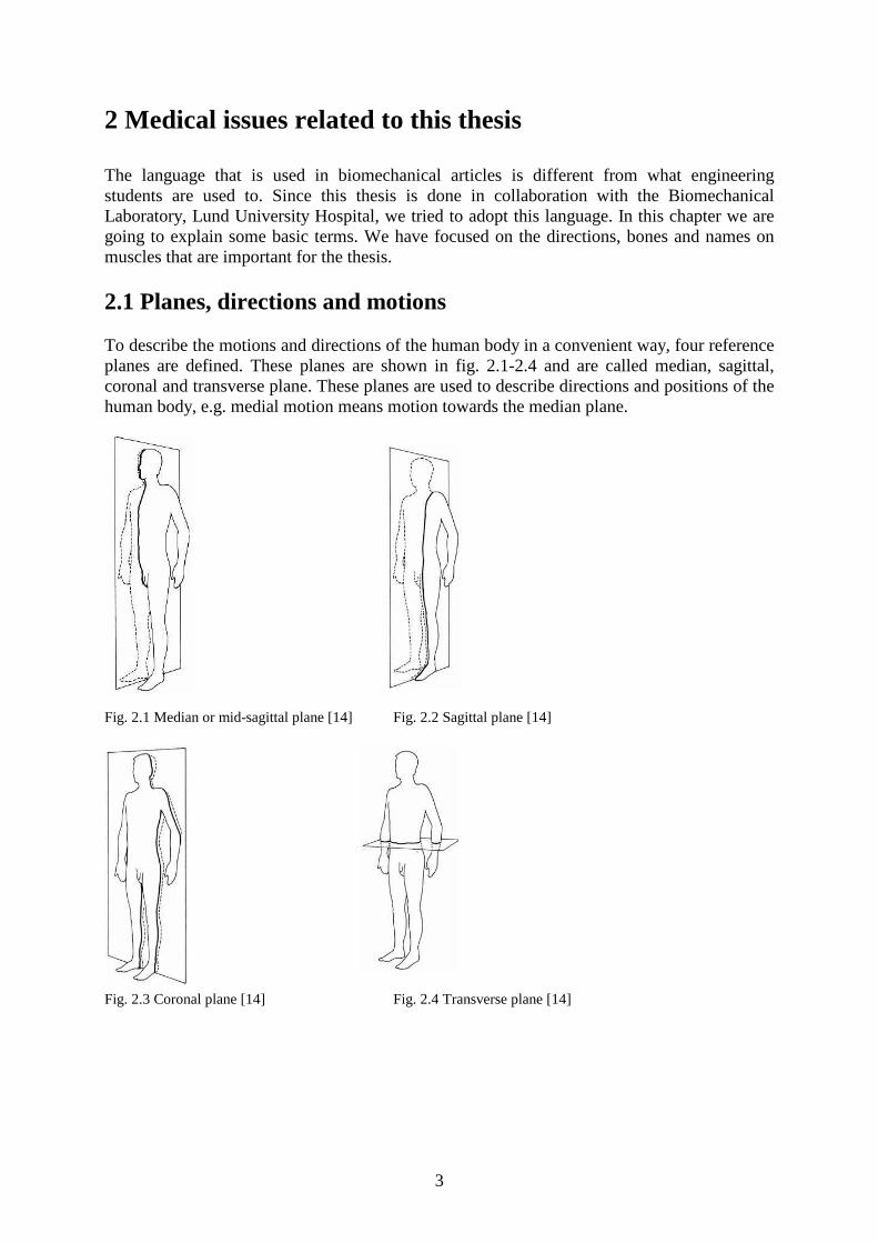
2.1 Planes, directions and motions To describe the motions and directions of the human body in a convenient way, four reference planes are defined. These planes are shown in fig. 2.1-2.4 and are called median, sagittal, coronal and transverse plane. These planes are used to describe directions and positions of the human body, e.g. medial motion means motion towards the median plane.

Fig. 2.1 Median or mid-sagittal plane [14] Fig. 2.2 Sagittal plane [14]

Fig. 2.3 Coronal plane [14] Fig. 2.4 Transverse plane [14]

4

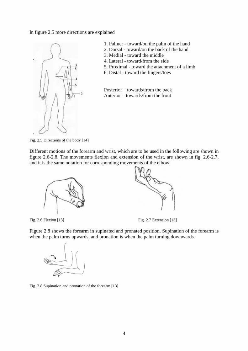
In figure 2.5 more directions are explained 1. Palmer - toward/on the palm of the hand 2. Dorsal - toward/on the back of the hand 3. Medial - toward the middle 4. Lateral - toward/from the side 5. Proximal - toward the attachment of a limb 6. Distal - toward the fingers/toes

Posterior – towards/from the back Anterior – towards/from the front

Fig. 2.5 Directions of the body [14] Different motions of the forearm and wrist, which are to be used in the following are shown in figure 2.6-2.8. The movements flexion and extension of the wrist, are shown in fig. 2.6-2.7, and it is the same notation for corresponding movements of the elbow.

Fig. 2.6 Flexion [13] Fig. 2.7 Extension [13] Figure 2.8 shows the forearm in supinated and pronated position. Supination of the forearm is when the palm turns upwards, and pronation is when the palm turning downwards.

�

Fig. 2.8 Supination and pronation of the forearm [13]

5

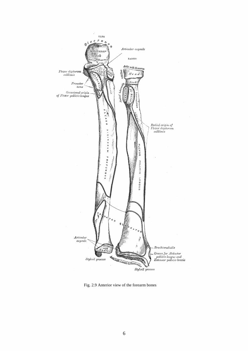
2.2 Bones of the forearm 2.2.1 Radius Radius is one of the two bones in the forearm. It is situated on the lateral side of the ulna, thumb side of the forearm. It is a long bone, prismatic in form and slightly curved longitudinally. It has a long body and two extremities. The proximal end, i.e. upper end, of the bone is small, and forms a small part of the elbow joint, but the distal end is large and forms the major part of the wrist joint. The distal part of the radius has two articular surfaces. One is the contact zone between the radius and the ulna, i.e. ulnar notch of the radius, and the other is the joint towards the hand. On the lateral side there is an outgrowth, the styloid process, which the tendon of the Brachioradialis, is attached to. 2.2.2 Ulna The second bone of the forearm, ulna, is a long bone parallel to the radius. Its proximal end forms a large part of the elbow-joint. But the distal end is very small and articulates with radius. It is excluded from the wrist-joint by an articular disk.

6

Fig. 2.9 Anterior view of the forearm bones

7

2.3 Muscles This section is a short presentation of the muscles that we have used when we estimated the forces for our testing. We have focused on the origin and the insertion of the muscles and their tasks. Brachioradialis is the most superficial muscle of the radial side of the forearm. The origin of the muscle is the proximal 2/3 of lateral supracondyle ridge of humerus (bone of the upper arm), and then it is inserted into the lateral side of the styloid process of the radius. This muscle is one of the major flexors of the forearm, it also supinates and pronates the forearm.

Fig. 2.10 Dorsal view of the right forearm, Brachioradialis [15]

The Flexor carpi ulnaris (FCU) lies along the ulnar side of the forearm. It has two heads, humeral and ulnar. The humeral head is attached in the medial epicondyle of the humerus and the ulnar head is attached in the medial margin of the olecranon and from the upper two-thirds of the dorsal border of the ulna. The muscle ends in a tendon, which is inserted into the pisiform bone, and is prolonged from this to the hamate and fifth metacarpal bones (bones of the middle hand). The Flexor carpi ulnaris flexes the wrist and adducts the hand.

Fig. 2.11 Palmer view of the forearm [15] The Flexor carpi radialis (FCR) arises from the medial epicondyle of the humerus. The tendon is inserted into the base of the second metacarpal bone, and sends a slip to the base of the third metacarpal bone. This muscle flexes the wrist and abducts the hand.

Lateral supracondyle ridge

Styloid process

8

The Extensor carpi ulnaris (ECU) lies on the ulnar side of the forearm. The origin of the muscle is in the lateral epicondyle of the humerus and from the dorsal border of the ulna, and it is attached at the ulnar side of the base of the fifth metacarpal bone. It extends and adducts the hand at the wrist joint.

Extensor carpi radialis longus (ECRL) arises from the lower third of the lateral supracondylar ridge of the humerus. It is inserted into the dorsal surface of the base of the second metacarpal bone, on its radial side. This muscle extends and abducts the hand at the wrist joint.

Fig. 2.12 Dorsal view,

Extensor carpi ulnaris [15] The origin of the Extensor carpi radialis brevis (ECRB) is at the lateral epicondyle of the humerus and is inserted into the dorsal surface of the base of the third metacarpal bone on its radial side. It extends and abducts the hand at the wrist joint.

Fig. 2.13 Dorsal view, Extensor carpi radialis longus [15]

Fig. 2.14 Dorsal view Extensor carpi radialis brevis [15]

9

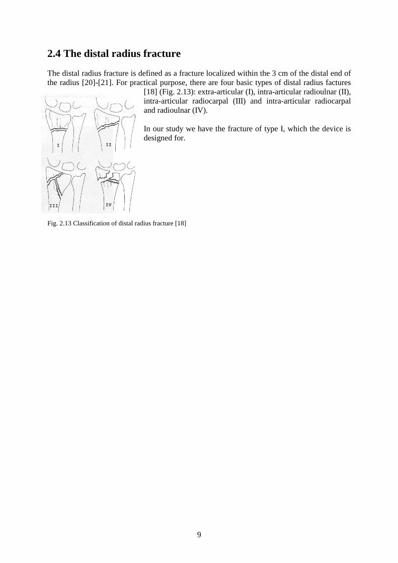
2.4 The distal radius fracture The distal radius fracture is defined as a fracture localized within the 3 cm of the distal end of the radius [20]-[21]. For practical purpose, there are four basic types of distal radius factures

[18] (Fig. 2.13): extra-articular (I), intra-articular radioulnar (II), intra-articular radiocarpal (III) and intra-articular radiocarpal and radioulnar (IV). In our study we have the fracture of type I, which the device is designed for.

Fig. 2.13 Classification of distal radius fracture [18]

10

3 General view of distal radius fracture fixation methods In the following chapter we will give you a short general view of some of the methods that are in use to fixate distal radius fractures. During the work, we have learnt that different methods are used for different types of fractures, and that there is no single best way to manage all fractures. But the basic principles are still the same:

• reduction of displaced fractures • maintenance of reduction during healing • restoration of hand and wrist function.

3.1 Cast With this method the surgeon returns the bones to their original place, and immobilizes the distal radius with a cast. This method of treating fractures of the distal radius is the most common one among stable fractures. Unstable fractures will often lose reduction in the cast and will slip back to the pre-reduction position. Complications such as joint stiffness and severe loss of muscle strength may appear after the removal of the cast.

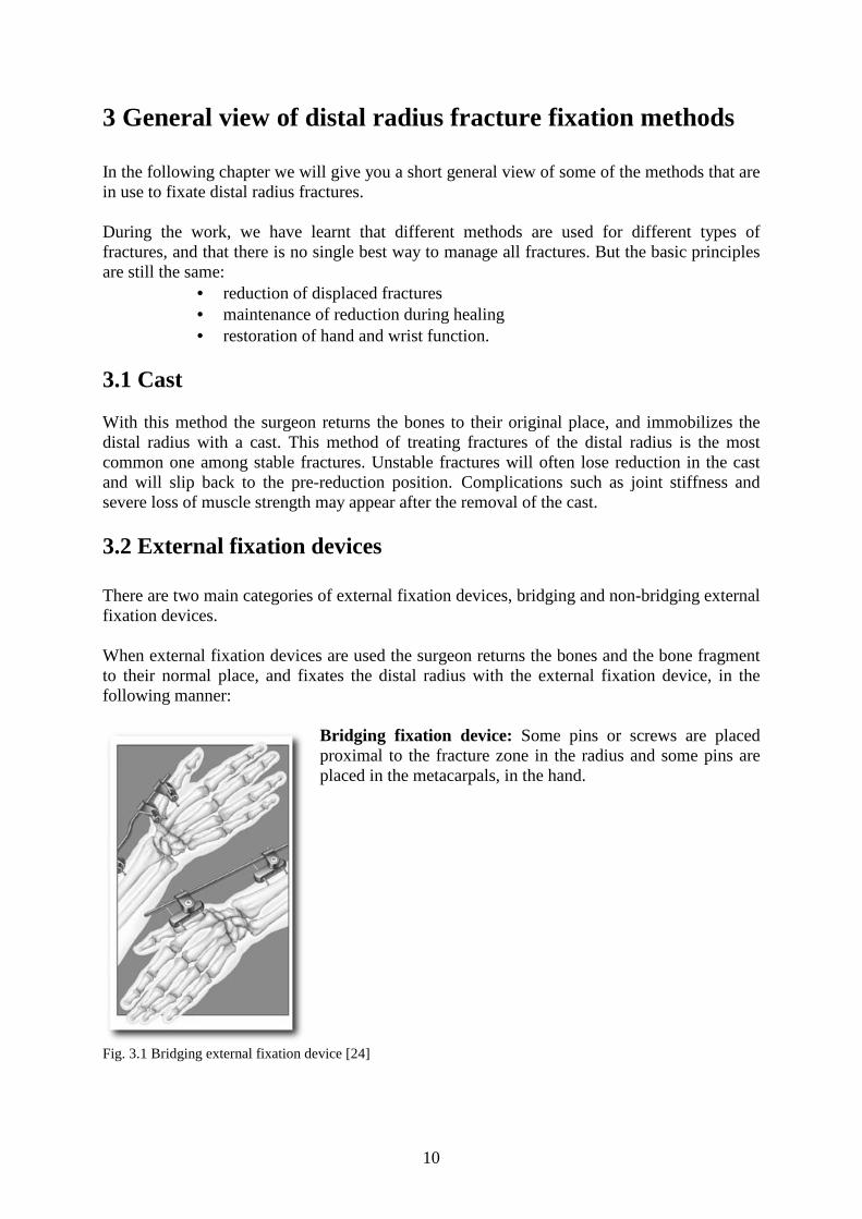
3.2 External fixation devices There are two main categories of external fixation devices, bridging and non-bridging external fixation devices. When external fixation devices are used the surgeon returns the bones and the bone fragment to their normal place, and fixates the distal radius with the external fixation device, in the following manner:

Bridging fixation device: Some pins or screws are placed proximal to the fracture zone in the radius and some pins are placed in the metacarpals, in the hand.

Fig. 3.1 Bridging external fixation device [24]

11

There are also bridging fixation devices including a joint, allowing early wrist motion to prevent prolonged immobilization. Hypothetically these devices are therefore better suited for intra-articular fractures than the classical external fixation devices [6]. In practice these methods have been unsuccessful due to the difficulties in reproduction of the complex kinematics of the carpus.

Fig. 3.2 Bridging external fixation device [25] Non-bridging fixation device: Some pins or screws are placed proximal to the fracture zone in the radius and some pins/screws are placed in the distal part of the radius and in the bony fragments of the fracture. With the non-bridging fixation device the wrist is allowed early wrist motion, to avoid joint stiffness.

Fig. 3.3 The non-bridging fixation device studied in this thesis, attached to two pieces of wood. With the external fixation device there is a risk that the tissue gets infected by the pins, i.e. pin track infection. There is also a risk of pin loosening if you fixate the bone with pins i.e. the pins loosen from the bone.

3.3 Internal fixation An internal fixation device placed through limited incisions on the posterior surface of the radius. It is placed across the fracture site and secured by screws to the radius and metacarpal. This eliminates the need for percutaneous pins. However, there is still no properly designed

12

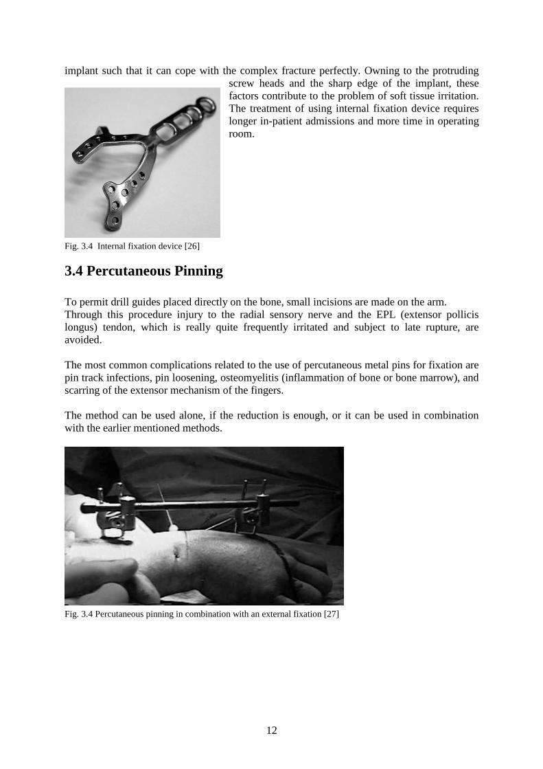
implant such that it can cope with the complex fracture perfectly. Owning to the protruding screw heads and the sharp edge of the implant, these factors contribute to the problem of soft tissue irritation. The treatment of using internal fixation device requires longer in-patient admissions and more time in operating room.

Fig. 3.4 Internal fixation device [26]

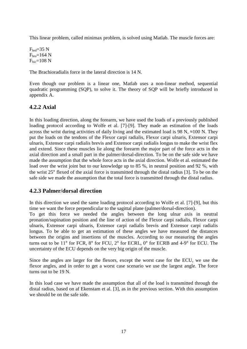
3.4 Percutaneous Pinning To permit drill guides placed directly on the bone, small incisions are made on the arm. Through this procedure injury to the radial sensory nerve and the EPL (extensor pollicis longus) tendon, which is really quite frequently irritated and subject to late rupture, are avoided. The most common complications related to the use of percutaneous metal pins for fixation are pin track infections, pin loosening, osteomyelitis (inflammation of bone or bone marrow), and scarring of the extensor mechanism of the fingers. The method can be used alone, if the reduction is enough, or it can be used in combination with the earlier mentioned methods.

Fig. 3.4 Percutaneous pinning in combination with an external fixation [27]

13

4 Loads Since the forearm is a very complex construction it is difficult to estimate the forces that the distal radius fixation device is exposed to. The loading of the fixator are estimated through qualified assumptions and calculations that will be stated in this chapter. The loading should be kept quite small, considering the radius has a fracture, and the normal reaction of the patient is not using the arm as much as usual because of the pain.

4.1 Pull out The cyclic loads that was applied on the Kirschner-wires (K-wires), described in chapter 5, are estimated through comparisons with the forces that one wire is exposed to in the arm during light activities of daily living. We came up with two different forces, based on the following facts. When a force in the wrist joint is transmitted through the forearm is, to our knowledge, up to 85 %, in neutral position and 92 % with the wrist 25° flexed, of the force transmitted through the distal radius [3]. But to be on the safe side we made the assumption that the total force is transmitted through the distal radius. The human hand corresponds to 0.006*body mass [1], and the mean body mass for a male in Sweden during the years 98-00 is 80.9 kg[2]. We used a body mass of 90 kg to get some margin and then the mass of the hand is 0.54 kg. The hand effects the distal radius with a force of 5.3 N and this force is divided into the three K-wires. Dividing this on the three K-wires will get a very small force (1.77 N). Movement of the hand exposes the K-wires to a larger force, due to acceleration, that we estimated to be approximately 5 N. The larger force in the cyclic loading is calculated from gripping and lifting a 0.4 kg glass of water, with the friction coefficient is approximated to 0.2 [37], the grip force turns out to be:

Ngmg

102.02

4,0

2≈

⋅=

µ (4.1)

Due to the lifting of the glass we get some acceleration. In order to compensate for this we double the force. According to Putnam et al. [4], 2.6 N is transmitted through the distal radius for every 1.0 N of grip force, this is when the arm is in neutral supination/pronation position. The force in the distal radius is then 52 N in our case, and the force in a K-wire is ≈20 N. The numbers of cycles we have chosen for the cyclic loading are 5000 cycles for the 5 N amplitude and 1000 cycles for the 20 N amplitude. If these cycles are summarized over the whole healing period (5 weeks) they turn out to give: 143 cycles/day (=6.0 cycles/hour) for the 5 N load and 29 cycles/day (=1.2 cycles/hour) for the 20 N load. This is our own estimations and we think they are a good approximation of the daily life of a recovering patient.

14

4.1.2 Estimation of needed pullout strength In this section a rough estimation of the forces the interference fit will have to withstand is performed. This is done with a very simple calculation of a rigid body. A moment equilibrium around wire 1:s insertion in the bone and a vertical equilibrium equation, gives us: Flat⋅80-Fw2⋅15-Fw3⋅30=0 (4.1) Flat- Fw1- Fw2- Fw3=0 (4.2) This problem is indeterminate, so a reduction was done. To be sure that we are on the safe side, we used the placement of wire2 for Fw2 and Fw3. Then eq. (4.1) will be: Flat⋅80-2⋅Fw2,3⋅15=0 (4.3) With the Flat presented in section 4.2.1, i.e. 14 N, Fw2.3 becomes 38 N and eq. (4.2) gives us Fw1=62 N. Fig. 4.1 Sketch of the lateral load case The axial loading case may give a worse case for the interference fit. The interference fit of angled wire in the distal bone fragment may have to withstand even larger forces, since our load in the axial direction, presented in section 4.2.2, is greater, 100 N. If you assume that the axial force is divided equal between the three wires in the distal bone fragment, the force the angled interference fit have to withstand is: (100/3)/sin(30)=67 N.

Flat

80

65

50

w1 w2 w3

(mm)

15

4.2 Loads for testing of the whole device Here we have used three load cases, as described in chapter 5: lateral-, axial- and palmer/dorsal direction. 4.2.1 Lateral direction The distal tendon of the Brachioradialis is inserted into the lateral side of the radius in the styloid process [5]. If there is a distal radius fracture the effect of Brachioradialis is critical. The Brachioradialis is one of the three major contributors to flexing the forearm, the other two are Biceps brachii and Brachialis. To estimate the force in the Brachioradialis we used a loading case, where the hand is exposed to a 20 N force with the arm flexed 90° and the forearm in neutral pronation/supination. Muscle PCSA (m2) r (m) θ (deg) Brachialis (bra) 4.6⋅104 0.034 80.3° Biceps brachii (bic) 7.0⋅104 0.046 68.7° Brachioradialis (brd) 1.5⋅104 0.075 23.0° PCSA=physiological cross section area, muscle volume/fiber length r=flexion-extension moment arm θ=angle between muscle force vector and long ulnar axis sagittal plane Fa=Force corresponding to mass of the arm. Fh= Force corresponding to mass of the hand. W=Force in the hand. J=Joint forces in the elbow.

400

150

Fh+W Fa

Fbrd

Fbic Fbra

Jy

Jx

Fig. 4.2 Free body diagram of a forearm in 90° flexion. The elbow at the left and hand at the right

θ

16

As earlier we used a body mass of 90 kg and the anthropometry information is collected from [1]. The moment equilibrium equation turns out:

0)(4.0)(20)(4.0)/(006.0)(90)(15.0)/(023.0)(90

)()(075.0)()(046.0)()(034.022 =⋅−⋅⋅−⋅⋅−

−⋅+⋅+⋅

mNmsmgkgmsmgkg

NFmNFmNFm brdbicbra

165.13075.0046.0034.0 =⋅+⋅+⋅ brdbicbra FFF (4.2)

This is a statically indeterminate problem and there are two widely used approaches to get a unique solution: reduction or optimization. Reduction methods seek to reduce the number of unknowns to equal the number of equations. In our case we use optimization. 4.2.1.1 Optimization We have chosen to do our optimization method according to An et al. [23]. This method uses that the endurance of the muscle system depends on each individual supporting muscle, the muscle that has the least endurance will be the key element for the system. And the assumption that muscle endurance is inversely proportional to the muscle stress. In addition to this an inequality condition was introduced, eq. (4.4) where the left side is the stress on the muscle and the right side is the upper bound for all of the muscle stresses. The result from this method has been compared with EMG data, by An et al. [23], and they match well. The problem may now be stated as:

Minimize σ Subject to:

�=

=n

iii FrM

1

(4.3)

σ≤i

i

PSCA

F (4.4)

To solve this problem we assume that Fi/PSCA i will be equal to σ. And we rewrite the problem as: Minimize (max Fi/PSCA i)

Subject to:

�=

=n

iii FrM

1

17

This linear problem, called minimax problem, is solved using Matlab. The muscle forces are: Fbrd=35 N Fbra=164 N Fbic=108 N The Brachioradialis force in the lateral direction is 14 N. Even though our problem is a linear one, Matlab uses a non-linear method, sequential quadratic programming (SQP), to solve it. The theory of SQP will be briefly introduced in appendix A. 4.2.2 Axial In this loading direction, along the forearm, we have used the loads of a previously published loading protocol according to Wolfe et al. [7]-[9]. They made an estimation of the loads across the wrist during activities of daily living and the estimated load is 98 N, ≈100 N. They put the loads on the tendons of the Flexor carpi radialis, Flexor carpi ulnaris, Extensor carpi ulnaris, Extensor carpi radialis brevis and Extensor carpi radialis longus to make the wrist flex and extend. Since these muscles lie along the forearm the major part of the force acts in the axial direction and a small part in the palmer/dorsal-direction. To be on the safe side we have made the assumption that the whole force acts in the axial direction. Wolfe et al. estimated the load over the wrist joint but to our knowledge up to 85 %, in neutral position and 92 %, with the wrist 25° flexed of the axial force is transmitted through the distal radius [3]. To be on the safe side we made the assumption that the total force is transmitted through the distal radius. 4.2.3 Palmer/dorsal direction In this direction we used the same loading protocol according to Wolfe et al. [7]-[9], but this time we want the force perpendicular to the sagittal plane (palmer/dorsal-direction). To get this force we needed the angles between the long ulnar axis in neutral pronation/supination position and the line of action of the Flexor carpi radialis, Flexor carpi ulnaris, Extensor carpi ulnaris, Extensor carpi radialis brevis and Extensor carpi radialis longus. To be able to get an estimation of these angles we have measured the distances between the origins and insertions of the muscles. According to our measuring the angles turns out to be 11° for FCR, 8° for FCU, 2° for ECRL, 0° for ECRB and 4-9° for ECU. The uncertainty of the ECU depends on the very big origin of the muscle. Since the angles are larger for the flexors, except the worst case for the ECU, we use the flexor angles, and in order to get a worst case scenario we use the largest angle. The force turns out to be 19 N. In this load case we have made the assumption that all of the load is transmitted through the distal radius, based on af Ekenstam et al. [3], as in the previous section. With this assumption we should be on the safe side.

18

5 Methods In all our tests wood, i.e. oak, has been used to simulate bone. We made up a few specifications for the test specimen together with our supervisors at Lund University Hospital.

• The distance between the wood pieces and the plate should be 10 mm. • The gap between the wood pieces should be 10 mm [19]. • The wood pieces should be aligned [19]. • The proximal end of the radius should be fully constrained [19].

The wood pieces used in the tests had a cross section of 20x20 mm, but the results has been recalculated to a bone analog with a cross section of 15x15 mm, since this is recommended by ASTM F 1541-01 [19]. In addition to the specifications we decided that the distance between the fracture surface and vertical K-wires should be 17 mm (fig. 5.1). This means that the distance between the fracture surface and the radial styloid process (see fig. 2.9) is approximately 20 mm, which is a distance that are commonly used to simulate distal radius fractures [7]-[9], [16]. According to [19] the bending stiffness of the bone analog should be 100 times the compression stiffness of the test specimen, and oak fulfills this criterion.

Fig. 5.1 Sketch of a specimen for tests of the whole device.

5.1 Pullout strength The main issue of the pullout tests was to decide the thickness needed to be sure that no sliding occurs in the contact between the plate and the wire. We tested four different thickness: 2, 3, 4 and 8 mm. The tests were interesting for this application but the designer was also interested in the tests in order to use this fixation method for other fractures (bones in the fingers for example) in the future. We did the pullout tests in three different manners:

• immediately after introduction of the wires. • after 5 weeks, i.e. healing time, storage at room temperature. • after 5 weeks storage at room temperature and cyclic loading perpendicular to the

wire. 5000 load cycles at 5 N and 1000 load cycles at 20 N all performed at 1 Hz. Four specimen of each thickness were used for each manner. Since this is a friction problem there are two different of pullout forces, one static and one dynamic. We are interested in the static pullout force, Fs, which is the maximum force applied before the equilibrium is violated. When the static pullout force is overcome, sliding occurs and then the dynamic pullout force, Fd, is the force needed for sliding to continue.

10 17

10

19

5.1.1 Preparing the test specimen The wires were pushed through the 1 mm holes. Since there is only axial loading to the wires in load case one we reused those wires after cleaning them with alcohol. We were careful not to touch the wires with our hands since grease from the fingers can decrease the pullout strength. 5.1.2 The cyclic loading The cyclic loading was performed with an Instron 8511 (with MTS controller) and a 500 N load cell. The load was applied at a 25 mm distance, in the axial direction of the wire, from the center of the plate. We had to use a special fixation of the device in order to apply the load.

Fig. 5.3 Cyclic loading of the test specimen

Fig.5.2 Typical pullout test

Fs

Fd

F

U

20

5.1.3 Pullout tests The pullout tests were performed the same way for the three different groups of specimen. The plate was fixated while an axial displacement controlled load was applied to the wire. The displacement rate in the pullout tests was 5 mm/min. The tests were performed using a Instron testing machine. The pullout tests of the cyclic loaded specimen were performed within 24 hours after the cyclic load was applied to avoid time effects.

5.2 Testing of the whole device The goal with testing of the whole device is to see if the displacement of the bone fragment is larger then 2 mm and if there is any permanent deformation of the device. Three tests were done, the device were loaded in three perpendicular directions, lateral, palmer/dorsal and axial. These tests were done with five specimens in each direction. 5.2.1 Preparing the test specimens The K-wires were driven through 1 mm holes, in the UHMWPE-plates, and into the bone analog, i.e. oak, with a drilling machine, this causes wearing of the contact surface on the UHMWPE-plate. 5.2.2 Testing in the lateral direction These tests were performed as a cantilever-bending test, which is the recommended [19] when you have a fixation system that is not symmetric over the fracture. The test specimen was rigidly anchored in the proximal end and unconstrained in the distal end, according to ASTM F1541-00 [19]. The displacements were measured in two directions, because of the symmetry of the fixation device, and then the total displacement was calculated. The displacements were measured in axial and lateral direction. The displacements were measured with resistive displacement sensors, see fig 5.4. Because of the measuring equipment used in the testing, it is not the exactly the same point on the bone analog that is measured during the testing. But the measuring equipment was placed, on the distal part, in such manner that when the fixation device was fully loaded the measuring point was the one that had the largest displacement. The loading in this direction should have been put on the styloid process, were Brachioradialis is inserted, but because of the measuring equipment this was not possible. To solve this, the loading point was moved in the distal direction. A hole was drilled in the bone analog 35 mm from the distal fracture surface, which is approximately 20-25 mm in the distal direction from the insertion of Brachioradialis. A wire with a ball in the end was used to pull the distal part of the bone analog, this was done at a speed of 0.5 mm/min. The insertion of Brachioradialis has a very small lever for bending moment around the K-wires in the distal bone, and our force has greater lever. This makes this a much worse case.

21

Fig. 5.4 Testing in the lateral direction

5.2.2 Testing in the Palmer/dorsal direction The testing of the device in the palmer/dorsal direction was also done as a cantilever bending test, with the proximal end rigidly anchored and the distal end unconstrained. Because there is no symmetry in this direction we measured the displacements in all of the three directions. The displacements were measured with resistive displacement sensors, see fig 5.5. The device was loaded in the same manner as in the lateral direction, pulled by the testing machine with a wire and a ball in a speed of 0.5 mm/min. The load was applied were the Flexor carpi radialis is inserted, which according to our measuring is 60 mm from the distal fracture surface.

Fig. 5.5 Testing in the palmer/dorsal direction

22

5.2.3 Testing in the axial direction Testing the device in the axial direction was done with the proximal end fully constrained and the load was put on the distal end. The load was applied with a rounded tip in the center of the distal end of the distal bone analog, the same loading speed as earlier, i.e. 0.5 mm/min, was used. The axial displacement was measured in the distal fracture surface with a resistive displacement sensor. The displacement in the lateral direction was calculated, this was possible since the loading speed and the loading time was known for the point were the load was applied. Loading the device in this manner is not ideal, because the rounded tip that the load was applied with slipped a little bit, approximately 1 mm in the lateral direction, on the distal surface. The fully constrained proximal end does not correspond with reality, but the displacements will be greatest on the distal side of the fracture. And this makes the measuring of the displacements much easier. The distal part of the bone analog was 35 mm, this is done so that the load in the axial and lateral direction is applied in the same point, in order to try to simulate the force of Brachioradialis.

Fig 5.6 Loaded in the axial direction

5.3 Finite element analysis It was not possible to apply the Brachioradialis force in the right place using the available testing equipment, so we had to use FE-analysis. In addition to this FEA made it possible to simulate fracture healing. In order to compare the results from the mechanical testing the loading in the axial and palmer/dorsal direction was analyzed. These analysis’s makes it easier to apply the load at the right place and it makes the measuring of the displacements much more simple.

23

5.3.1 Creating the FE-model The 3D-model was created in Pro Engineer and exported to Hypermesh. The fixation device was modeled almost as it looks in reality except that the plate has constant thickness in the model. We strongly feel that the difference of the thickness between reality and model has a minor importance since it appears in parts of the plate that does not contribute much to the stiffness of the whole device. By doing this simplification we are able to improve mesh quality. Since every human radius has individual design and in order to get a better mesh, the bone model is simpler than in reality. Another reason for the simple bone model is that we are not interested in bone stresses and with this change we get a lower time cost for the analysis. The bone model has a square shaped cross section with a thickness of 15 mm. There is a widening of the cross section in the distal part, this is a result from early attempts to make the bone model look more like reality. The widening does not matter for the results. The model was meshed using Hypermesh software, and the mesh was created with eight node hexagon elements. The load and boundary conditions as well as the contact surfaces between the plate and the wires were defined in Hypermesh. Since the project was limited to not analyze the contact between the wires and the bone we modeled this contact as easy as possible and tied the nodes together.

Fig. 5.7 The mesh used in the axial, brachioradialis and axial-healing load cases.

24

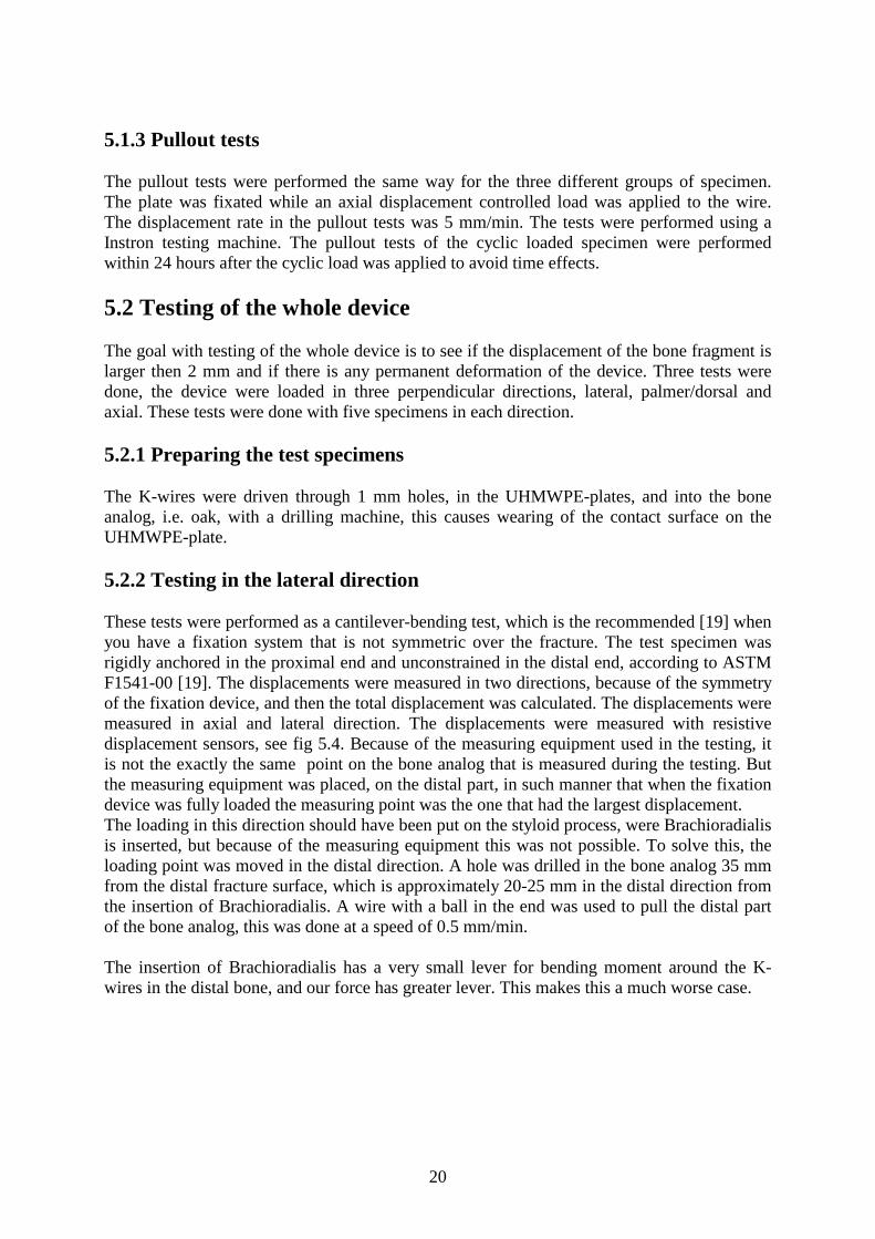
Fig. 5.8 The mesh used in the Palmar/dorsal load case. 5.3.2 The contact problem The contact surfaces between the pins and the fixation plate were defined in Hypermesh. The wire surfaces are defined as master surfaces and the plate surfaces are defined as slave surfaces. This means that the nodes on the plate surfaces cannot penetrate the wire surfaces but the wire surfaces can, in principle, penetrate the plate surfaces. The choice of which surface to be the master surface is done according to the ABAQUS user manuals. There it is recommended to choose the stiffer body as the master surface. Since the wire and the plate are in contact in the beginning of the simulation and since there is a big over closure, we had to solve the contact problem before we could apply any other loads. The contact problem was solved with the automatic “shrink” fit method in ABAQUS, which shrinks the slave surface onto the master surface using a default amplitude curve, a linear ramp to zero. To account for the relative motion of surfaces in the contact simulation small-sliding formulation were used. The small-sliding formulation assumes that the surfaces may undergo arbitrary large rotations but that a slave node will interact with the same area of the master surface throughout the analysis [36]. The reason to use small-sliding contact is that it is less expensive computationally than finite-sliding contact. 5.3.3 Mechanical properties We have been unable to find the material properties for stainless steel [ISO 5832-1] so we have chosen a typical value for stainless steel. The coefficient of friction used in the contact between the wires and the plate is 0.1 [31]. Steel Bone UHMWPE Youngs' modulus (GPa) 220 17 Poissons' ratio 0.3 0.4 0.45 Table 5.1 Material properties. [12],[32],[33] Youngs’ modulus for UHMWPE is presented in chapter 6.

25

5.3.4 Boundary conditions The degrees of freedom of the nodes on the proximal end of the radius that correspond to all translations were locked. 5.3.5 Loading All loads used in the FE-simulation are presented and motivated in chapter 4. The directions are shown in fig 5.7, direction 1 is palmer/dorsal, direction 2 is axial and direction 3 is radial. The displacements were measured on the distal fracture surface. In all cases except for the palmer/dorsal load case the displacements are measured in the middle node of the fracture edge on the radial side and the fracture edge on the ulnar side. This is enough to describe the displacement of the fracture surface since the loads and the structure are symmetric. In the palmer /dorsal load case the bone fragment is twisting and therefore not symmetric, the largest displacements will be on the palmer/dorsal fracture edges. 5.3.5.1 Axial load case The first load case was to apply an axial 100 N load. The load was applied as a distributed load on the distal surface of the radius, 20 mm from the distal fracture surface. 5.3.5.2 Brachioradialis load case The second load case were the Brachioradialis muscle, the force was applied between the fracture and the pins in the distal bone fragment. It is placed in the middle of the radial side of the fragment, 12 mm from the fracture surface (i.e. at the first node proximal to the middle K-wire). 5.3.5.3 Palmer/Dorsal load case The force was applied 60 mm from the fracture surface in the palmer dorsal direction. It was distributed over the central cross section in palmer/dorsal direction.

26

6 Constitutive model for UHMWPE We did the judgment that the best way to describe was to use a hyperelastic material model, which is a non-linear elastic model, for the instant behavior and a viscoelastic model for the time dependent behavior.

6.1 Testing the material In the ABAQUS manuals there are several tests described to perform in order to get the data needed to calibrate a hyper-elastic material model. It is preferred to do as many as possible of these different types of test but because of the difficulties of performing some tests and the test equipment available, we were only able to do one type of test. We also had to do one test to get data to the viscoelastic model. In order to get data for the material behavior we performed:

• uniaxial tension test • creep test

Both the uniaxial test and the creep test were performed on test specimen designed as described in standard SS 112116. The uniaxial test was displacement controlled and done at the speed of 200 mm/min to avoid time dependent effects. This strain rate is the maximum speed of the test equipment that we used. We did four identical tests with four specimens to be sure that the test data was representative for the material. Maybe it would have been interesting to do a uniaxial test at a lower speed to compare and see the time dependent effects but, as mentioned earlier, we had a limited number of test specimen. The creep test was performed with constant load of the test specimen during 24 hours. We did the test at three different load levels. The size of the load was determined after some simple calculations in order to estimate the stress in the middle part of the plate when it is applied to a fractured radius. The first load level was below, the second just about and the third over.

6.2 Creating the constitutive material model We tried to calibrate the predefined hyper-elastic material forms that are available in ABAQUS to our test data but we could not get a good fit. Because of the large deformations around the holes, a good fit both for small and for large deformations in tension and compression was necessary. Instead of using a hyper-elastic model we did the choice to use an elastic-plastic model. We defined a two-step linear plasticity using a “classical metal plasticity model” , which enabled a good fit. Since we do not have any test data for unloading we modelled it as perfect plasticity which means that no hardening occurs. Perfect plasticity is the default option in ABAQUS. The hardening behavior is not interesting, in these analyses, since no unloading will be performed.

27

Fig. 6.1 UHMWPE material model. Youngs modulus= 502 MPa First step plastic starts 19.2 MPa and after 0.05 plastic strain perfect plasticity starts at 24 MPa.

6.3 Creep test data Creep tests of the UHMWPE were performed since it tends to creep, but the results were not used in our analysis. Since only static analyses were performed, where viscoelastic effects are not considered, no creep test data were used in the analyses. We did not feel confident that the results would describe the behavior in the large plastic strain zones around the holes since the stress levels in the tests where predictions of the bending stresses of the plate. The results from the creep test are presented in Appendix B.

*=test data -=material model

28

7 Fracture healing Fracture healing involves tissue generation inside and in the surroundings of the site of the injury.

Fig 7.1. Intact bone. [10]

7.1 Primary healing Healing begins as undifferentiated mesenchymal cells migrate from the surroundings and produce initial connective tissue around the fracture site, forming an initial stabilizing callus [10]. This is called primary healing and occurs in cases of extreme stability and negligible gap size [10].

7.2 Secondary healing In most cases, which involve moderate gap size and stability, healing occur by so called secondary fracture healing [10]. During this healing process, the localized differentiation of the mesenchymal cells into cartilage and bone forming cells, lead to the production of cartilage and bone in the callus, in successful healing the initial connective tissue and cartilage are eventually replaced by bone [10]. Secondary healing is generally divided into four stages (I) inflammation, (II) callus differentiation, (III) ossification and (IV) remodeling. 7.2.1 The first stage Inflammation occurs immediately after bone rupture, when blood quickly fills the space of the fracture gap. Platelets and thromboic factors produce a connective fibrin tissue matrix.

29

Fig, 7.2. Inflammation. [10] 7.2.2 The second stage Blood cells migrate to the fracture site and promote the formation of a matrix, substrate necessary for the migration of mesenchymal cells. Mesenchymal cells originate from surrounding tissues. These cells replace the fibrin matrix by a new connective matrix and form the initial callus. The second stage proceeds with the formation of cartilage and bone, within the first 24 hours [10], along the bone mesenchymal cells differentiate into osteblasts which begin to synthesize bone.

Fig. 7.3. Callus differentiation. [10] 7.2.3 The third stage In the interior of the initial callus and adjacent to the bone, at approximately day 7, mesenchymal cells differentiate into chondrocytes which synthesize cartilage. At 10-12 days post-fracture, ossification of the cartilage callus begins, a process known as endochondral ossification [10]. This is the beginning of the third healing stage that ends at the point of bone formation. Endochondral ossification continues until all cartilage has been replaced by bone and an entirely bony bridge closes the fracture gap [10].

30

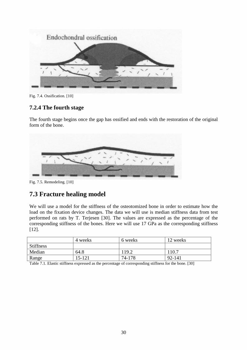
Fig. 7.4. Ossification. [10] 7.2.4 The fourth stage The fourth stage begins once the gap has ossified and ends with the restoration of the original form of the bone.

Fig. 7.5. Remodeling. [10]

7.3 Fracture healing model We will use a model for the stiffness of the osteotomized bone in order to estimate how the load on the fixation device changes. The data we will use is median stiffness data from test performed on rats by T. Terjesen [30]. The values are expressed as the percentage of the corresponding stiffness of the bones. Here we will use 17 GPa as the corresponding stiffness [12]. 4 weeks 6 weeks 12 weeks Stiffness Median 64.8 119.2 110.7 Range 15-121 74-178 92-141 Table 7.1. Elastic stiffness expressed as the percentage of corresponding stiffness for the bone. [30]

31

Fig. 7.6. The stiffness plotted from the data presented in table 7.1

The model will be used as springs in the FE analysis, we will use four symmetrically placed springs fixed to the fracture surfaces. The total spring constant Ks will be calculated as Ks=F/dL=E*A/L (7.1) Where E=Young’s modulus for median of the stiffness data, A=the area of the fracture surface and L=the initial fracture gap in the FE model. The spring constant will then be divided into four and applied to each spring. This is a simplification of reality and it will only prevent displacement in axial direction and we will only use it on the axial load case. The fixation device is removed five weeks after it is applied so it is only the first five weeks that we are interested in. Since measurements of the stiffness was performed in the fourth, sixth and twelfth week, we decided to use the results from the fourth week. The median stiffness in week four are 64.8 % of corresponding value of control bones. So Young’s modulus as 17 GPa, the fracture area as 176.7 mm2 and the fracture gap as 7.75 mm (7.1) give us Ks ≈251 kN/mm. Then we divide Ks on four springs and get 62.8 kN/mm.

32

8 Results & Discussion 8.1 Pullout test 8.1.2 Pullout immediately after introduction

2 mm 3 mm 4 mm 8 mm Test Force (N) Force (N) Force (N) Force (N)

1 31 38 47 108 2 25 42 55 114 3 27 41 47 100 4 45 46 87

Mean value 27.67 41.5 48.75 102.25 Standard dev. 3.06 2.89 4.19 11.67

Table 8.1. Pullout test results immediately after introduction of the pins (K-wires).

Fig. 8.1. Pullout strength, immediately after introduction of the pins (K-wires), plotted against thickness of the plate.

Since the results from the tests are pretty close to each other for the specimens of the same thickness the authors feel sure that four tests are enough to get good results. Another argument for this statement is the almost linear plot.

33

8.1.3 Pullout strength after 5 weeks storage

2 mm 3 mm 4 mm 8 mm Test Force (N) Force (N) Force (N) Force (N)

1 20 30 46 87 2 28 27 38 103 3 29 35 45 106 4 26 28 41 96

Mean value 25.75 30 42.5 98 Standard dev. 4.03 3.56 3.70 8.45

Table 8.2. Pullout test results 5 weeks after introduction of the pins (K-wires).

2 mm 3 mm 4 mm 8 mm Force (N) -1.92 -11.5 -6.25 -4.25

% -6.93% -27.71% -12.82% -4.16% Table 8.3. Change in pullout strength after five weeks storage.

Fig. 8.2. Pullout strength 5 weeks after introduction of the pins.

The change in grip strength after five weeks is not that considerable except for the 3 mm plates. The authors have no easy explanation for the difference in behavior between the 3 mm specimen and the other specimen. There has not been any special treatment of the 3 mm specimen.

34

8.1.4 Pullout strength after 5 weeks and cyclic loading

2 mm 3 mm 4 mm 8 mm Test Force Force Force Force

1 24 28 37 84 2 10 25 44 88 3 23 27 35 97 4 26 27 90

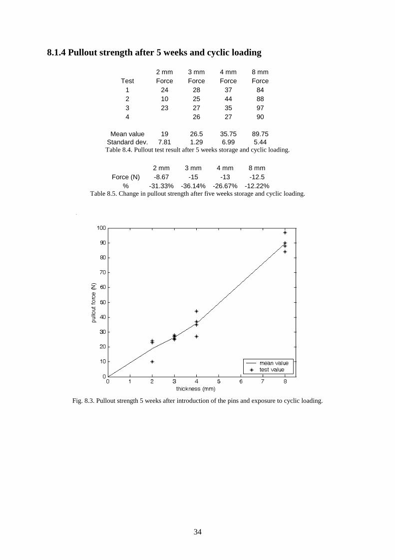
Mean value 19 26.5 35.75 89.75 Standard dev. 7.81 1.29 6.99 5.44 Table 8.4. Pullout test result after 5 weeks storage and cyclic loading.

2 mm 3 mm 4 mm 8 mm

Force (N) -8.67 -15 -13 -12.5 % -31.33% -36.14% -26.67% -12.22%

Table 8.5. Change in pullout strength after five weeks storage and cyclic loading.

Fig. 8.3. Pullout strength 5 weeks after introduction of the pins and exposure to cyclic loading.

35

Fig. 8.4. Mean values of pullout tests. Data 1 is from tests performed immediately after introduction. Data 2 is from tests performed five weeks after introduction. Data 3 is from tests performed five weeks after introduction and exposure to cyclic loading.

From these results one can see that the thicker specimen is better suited to withstand cyclic loading. This is probably due to the larger contact area of the interference fit. 8.1.5 Discussion Friction force depends linear on three parameters: coefficient of friction, pressure and contact area. The only parameter that changes here is the contact area, which changes linear with thickness, since plates of different thickness are investigated. Ff=pAµ where A=2πrt So the result where the pullout strength turns out as a linear function of thickness was not surprising. The difference in pullout strength between group one, two and three is not very large. We did some tests with wires that we had touched with our fingers and the grip strength is in average 36 % lower. We do not know how much of the contact surfaces that was greased and the change in the strength of the grip differ between the wires, but we think that the difference in grip strength shows the importance of clean wires. Since the K-wires were pushed through the UHMWPE-plates and not drilled through it, there is a lower amount of wear of the plates here. This might create a slight overestimation of the pullout strength.

36

8.2 Mechanical testing of the whole device All the results, except permanent deformations, are recalculated to a 15x15 mm bone analog. The permanent deformations are measured on the edge of bone analog, cross section 20x20 mm, this means that these are a little bit overestimated, but it still shows if there are permanent deformations or not. 8.2.1 Lateral direction

Fig. 8.5 Result from lateral test 1

Permanent deformation after unloading the fixation device: 0.48 mm (on the 20x20 mm bone analog)

___ Force ___ Displacement

37







38







39

Fig. 8.10 Mean displacement

Force (N) 4 8 12 14 Displacement (mm) 0.30 0.72 1.25 1.52 Standard dev. (mm) 0.0138 0.0793 0.166 0.218 Table 8.6 Distribution of displacements Mean permanent deformation: 0.43 mm (SD=0.228 mm) (on the 20x20 mm bone analog) 8.2.1.1 Discussion By looking at the test results from the testing in the lateral direction one can see that there are some jumps in the curves from test 1, 3 and 4. This is due to sliding between the K-wires and the UHMWPE-plate. This occurred on the proximal side of the fracture. Sliding first occurred at the most distal K-wire in the proximal bone analog (wire 3). But this loading case does not really correspond with reality, because we applied our force more distal then what the force of the muscle Brachioradialis does in real life. In lateral test 3 slipping occurs at 11.15 N, which is less than the load we estimated for daily living, but we have to consider that the moment arm is longer than in reality. To get an estimation of the force the interference fit have to withstand, the rigid body model in section 4.2.1 is used. In worst case, moment around wire 1 (see fig. 4.1), the moment arm in our tests will be approximately 133% of the moment arm in reality. If we use the 11.15 N that slipping occurred at to calculate the force that the interference fit have to withstand, eq. (4.2)-(4.3) it turns out to be Fw2,3=29.7 N and Fw1=48.3 N. The force where sliding occurs in the lateral testing should not be a problem according to our pullout tests. This is probably due to the difference in methods used when the K-wires are inserted in the plates. If we only consider the moment, which is the main contribution to the pullout force, and not the shear force, we can recalculate the force needed to withstand in our point of loading. The force to get the same moment around wire 1 (fig. 4.1) in our point of loading as one get when

40

14 N is applied on the insert of Brachioradialis is 14/1.33=10.5 N, which is smaller then the force where sliding occurs. The permanent deformation is considerably larger when sliding has occurred, which is not surprising. This is a reminder of how important it is that no sliding may occur. When loading the fixation device in this way bending occurs in three positions: the proximal K-wires, the fixation plate and the distal K-wires. In the first two positions we think that our tests is rather close to the reality, but a little bit overestimated. In the third position where bending occurs our way of loading the fixation device gives a bad estimation. This is due to the moment arm, which is to long and on the wrong side of the distal K-wires. The total displacements of the bone analog are larger in our tests then they will be in reality. The point were the load was applied in our tests was the closest to reality with the equipment used. 8.2.2 Palmer/dorsal direction

Fig. 8.11 Result from palmer/dorsal test 1



41







42







43

Fig 8.16 Mean displacement

Force (N) 5 10 15 19 Displacement (mm) 0.49 1.13 1.84 2.50 Standard dev. (mm) 0.0455 0.0722 0.157 0.207 Table 8.7 Distribution of displacements Mean permanent deformation: 0.40 mm (SD=0.187 mm) (on the 20x20 mm bone analog) 8.2.2.1 Discussion In this load case no sliding occurs, this is not surprising considering the direction of the load. Comparing the permanent deformation to the tests of the previous load case were no sliding occur, the permanent deformation in this case is rather large. Due to the lack of symmetry we expected displacements in three directions, but the displacement in lateral direction was very small.

44

8.2.3 Axial direction When performing the first test in the axial loading direction, the displacement sensor used to measure axial displacement of the fracture surface was damaged. That is why there only are four results shown.

Fig. 8.17 Result from axial test 2





45








46

Fig. 8.21 Mean displacement

Force (N) 25 50 75 100 Displacement (mm) 1.46 2.50 4.01 6.14 Standard dev. (mm) 0.312 0.362 0.541 0.460 Table 8.8 Distribution of displacements Mean permanent deformation: 0.69 mm (SD=0.147 mm) (on the 20x20 mm bone analog) 8.2.3.1 Discussion By looking at the test results from the testing in the axial direction one can see that there are sliding in test 2, 4 and 5. This occurred on the angled K-wire on the distal side of the fracture. Due to our testing equipment the measuring of permanent deformation in lateral direction was not possible. So the permanent deformation shown in this section is only in axial direction. Of course, the total displacement are larger but the axial displacement shows that there are permanent deformations. However, if permanent axial displacement is large, so will also the total displacement turn out to be large. On test 3 and 4 something happens with the force at approximately 25 N, we have no explanation for this phenomenon. This does not seem to affect the rest of the curve, so we do not think it is of great importance for the evaluation.

47

8.2.4 Brachioradialis direction

Fig. 8.22 Displacement due to Brachioradialis

8.2.4.1 Discussion In this section we have tried to estimate the displacement caused by Brachioradialis, by superposing the displacements caused by the forces in axial and lateral directions. The errors from the lateral testing gives an underestimation of the displacement, since the displacements of the lateral testing are in the wrong direction, due to the moment arm. The displacements from the lateral tests and the axial tests act against each other, this is not the case in reality.

8.3 Finite element analysis The loads vary linear from 0 to maximum load over a time step from one to two in these plots. This is because ABAQUS applies the load in time steps. Step 1 (0-1) is the contact analysis, this is to get an initial equilibrium in the interference fit and do not create any considerable displacements and therefore are not plotted. When comparing contact analysis to reality, This step corresponds to inserting the K-wires into the UHMWPE-plate. Step two (1-2) is when the loads apply and the corresponding displacements are shown below. The unit for the displacement magnitude is mm.

48

8.3.1 Axial loading

Fig. 8.23 Total displacement of fracture edge nodes plotted against time.

Fig 8.24 Displacement of fracture edge nodes in axial direction. The results from the axial load analysis give a total displacement of 6.2 mm on the ulna side of the fracture and 3.0 mm on the radial side (fig. 8.23). If one compare this result with the results from the mechanical testing (fig. 8.21), where the displacement was 6.14 mm, one can see that displacements are almost the same. This is a little bit surprising since sliding occurs in the mechanical test. The reason why sliding occurs in the mechanical tests and not in the FE-analysis is probably because of the wearing of the plate while inserting the K-wires. There is also a difference in length of the cross section edges which gives a 2.5 mm extra moment arm (20 mm instead of 17.5 mm). The length of the distal bone analog is 15 mm longer in the

49

mechanical testing then it is in the FE-analysis, this gives an small difference of the displacements compared with reality. The axial displacement is shown alone so one can compare with the simulated healing (fig. 8.28). 8.3.2 Palmer/Dorsal load case

Fig. 8.25 Total displacement of the fracture edge nodes in the palmer/dorsal load case.

The maximum displacement when the palmer/dorsal force is applied to the fixation device is 1.6 mm on the ulnar side and 1.1 mm on the radial side. The displacement in this analysis is smaller then the displacements in the mechanical tests (2.50 mm in mechanical tests).

50

8.3.3 Brachioradialis force

Fig. 8.26 Total displacement of the fracture edge nodes in the brd load case.

The maximum displacement when the Brachioradialis force is applied to the fixation device is 1.3 mm on the ulnar side and 0.79 mm on the radial side. This displacement is larger then the one we got by superposing the mechanical tests, this is not surprising since that the displacements in the mechanical tests are underestimated (see section 8.2.4.1). The main difference between the FE-analysis and the mechanical tests is that the force is put on the correct place for the Brachioradialis muscle in the FE-analysis.

51

8.3.4 Axial load case with springs to simulate healing

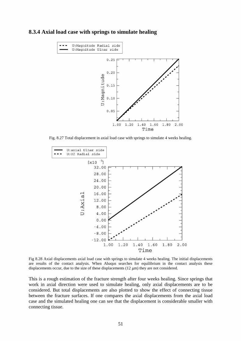
Fig. 8.27 Total displacement in axial load case with springs to simulate 4 weeks healing.

Fig 8.28 Axial displacements axial load case with springs to simulate 4 weeks healing. The initial displacements are results of the contact analysis. When Abaqus searches for equilibrium in the contact analysis these displacements occur, due to the size of these displacements (12 � m) they are not considered.

This is a rough estimation of the fracture strength after four weeks healing. Since springs that work in axial direction were used to simulate healing, only axial displacements are to be considered. But total displacements are also plotted to show the effect of connecting tissue between the fracture surfaces. If one compares the axial displacements from the axial load case and the simulated healing one can see that the displacement is considerable smaller with connecting tissue.

52

9 Conclusion With our load estimation in mind and the fact that the healing fracture can handle more and more load during the healing period, we do not think that creep effects or fatigue in the contact will be a problem during the healing process. Our load estimations and the results from the pullout tests indicate that the 8 mm specimens are likely to perform well in daily living. But the sliding in the lateral load case indicate that sliding occur at a lower load and we think this is due to wear while inserting the K-wires. When inserting the wires into the bone one should try to minimize the drilling, in order to minimize the wear of the UHMWPE-plate, since the wear is depending on the wear distance [22]. One way might be to push the K-wires through the holes as far as possible before drilling. Another way to increase the pullout strength might be to chose a different material for the fixation plate, since the UHMWPE-plate has a low yield strength and low coefficient of friction. If this is done the contact pressure will be increased, both this and the higher coefficient of friction would increase the pullout strength. The advantage with the UHMWPE is that it has a high wear resistance. The mechanical tests and the FE-analysis indicates that the fixation device will not be able to meet the requirements specified in section 1.3, i.e. to maintain reduction of the fracture during the healing period and no permanent deformations. In the estimation of the axial and the palmer/dorsal loads we overestimated the loads, since we made the simplification that everything was transmitted through the distal radius. But even if we take this in mind that 85 % of the force is transmitted through the distal radius, with the hand in neutral position [3], the load in the axial direction will cause to large displacements. The FE-analysis strengthens this conclusion. The testing in palmer/dorsal direction might meet the requirements, due to the overestimation of the force. We think that the fixation device will be able to fulfil the elastic requirements when loaded by Brachioradialis, based on the FE-analysis and mechanical testing in lateral direction. The mechanical tests show that there are permanent deformations after unloading the fixation device. One critical point of the design of the fixation device is the placing of the distal K-wires, it has a low bending stiffness if loaded in the axial and lateral direction. This bending stiffness would increase if they were not inserted in the bone on a line perpendicular to the axial direction, but this may not be possible considering medical issues. The stiffness of the device would also increase with increased diameter of the K-wires.

53

References [1] http://engineering.cua.edu/biomedical/courses/be398/com.html, 2003-01-20 [2] http://www.scb.se/statistik/le0101/le0101%5Fviktolangd.asp, 2002-12-03 [3] af Ekenstam FW, Palmer AK, Glisson RR. The load on the radius and ulna in different positions of the wrist and forearm. Acta Orthopaedica Scandinavia, 55:363-365, 1984. [4] Putnam MD, Meyer NJ, Nelson EW, Gesensway D, Lewis JL, Distal radial metaphyseal forces in an extrinsic grip model: Implications for postfracture rehabilitation. Journal of hand surgery, 25A:469-475, 2000 [5] http://www.bartleby.com/107/125.html, 2003-02-05 [6] van Dijk JP, Laudy FGJ. Dynamic external fixation versus non-operative treatment of severe distal radial fractures. Injury, Vol 27: 57-61, 1996 [7] Wolfe SW, Swigart CR, Grauer J, Slade JF, Panjabi MM, Augmented external fixation of distal radius fracture: A biomechanical study. Journal of hand surgery, 23A:127-134, 1998 [8] Wolfe SW, Lorenze MD, Austin G, Swigart CR, Panjabi MM, Load-displacement behaviour in a distal radius fracture model. Journal of bone and joint surgery, 81A:53-59, 1999 [9] Higgins TF, Dodds SD, Wolfe SW, A biomechanical analysis of fixation of intra-articular distal radial fractures with calcium-phosphate bone cement, Journal of bone and joint surgery, 84A:1579-1586, 2002 [10] Bailon-Plaza, A. & van der Meulen, M.C.H. (2001). A mathematical framework to study the effects of growth factor influences on fracture healing. J. theor. Biol. 212, 191-209 [11] Claes, L.E. & Heigele C.A. (1999). Magnitudes of local stress and strain along bony surfaces predict the course and type of fracture healing. J. Biomechanics 32, 255-266 [12] Fung, Y.C. (1993) second edition, Biomechanics: Mechanical properties of living tissues, Springer-Verlag New York [13] http://www.sportsmed.buffalo.edu/info/navicular2.html, 2003-04-06 [14] http://www.sci.port.ac.uk/rad/anatomy/, 2003-04-06 [15] http://www.rad.washington.edu/atlas/brachioradialis.html, 2003-04-07 [16] Dodds SD, Cornelissen S, Jossan S, Wolfe SW, A biomechanical comparison of fragment-specific fixation and augmented external fixation for intra-articular distal radius fractures. Journal of hand surgery, 27A:953-964, 2002 [17] Sobotta J. Atlas of human anatomy, volume 1, Head , neck, upper limb. Urban & Fisher, Munich, 13th English edition, 2001 [18] Gausepohl T, Pennig D, Mader K, Principles of external fixation and supplementary techniquesin distal radius fractures. Injury, 31:56-70,2000 [19] ASTM F1541-00 Standard specification and test methods for external skeletal fixation devices [20] Bacorn RW, Kurtzke JF, Colles’ fracture: A study of two thousand cases from the New York state workman’s compensation board. Journal of bone and joint surgery, 35:643, 1953 [21] Boyd LG, Home JG, The outcome of fractures of the distal radius in young adults. Injury, 19:97, 1988 [22] Jacobson B. Maskinelement Tribologi AK, Lund 1999 [23] An KN, Kwak BM, Chao EY, Morrey, Determination of muscle and joint forces: A new technique to solve the indeterminate problem. Journal of biomechanical engineering, vol 106: 364-367, 1984 [24] http://ortho.smith-nephew.com/ca_en/Category.asp?NodeId=355, 2003-05-18 [25] http://www.davidlnelson.md/distalradius.htm, 2003-05-18 [26] http://www.hku.hk/ortho/ortho/newsletter/newsletter03/6.html, 2003-05-18 [27] http://www.hwbf.org/ota/bfc/trum2/exp.htm, 2003-05-18

54

[28] ABAQUS /Standard user’s manual, vol I, version 6.3, Hibbitt, Karlsson & Sorensen, Inc 2002 [29] ABAQUS /Standard user’s manual, vol II, version 6.3, Hibbitt, Karlsson & Sorensen, Inc 2002 [30] Terjesen T. Fracture healing and stress-protection after metal plate fixation and external fixation. Publication from the University of Trondheim, Faculty of Medicine, Department of Ortopaedic Surgery, Trondheim University Hospital, Trondheim. 1984 [31] http://www.goodfellow.com/csp/active/static/A/ET30.HTML, 2003-05-18 [32] Otto JK, Callaghan JJ, Brown TD. Contact mechanics influences on interface mobility of a rotating platform total knee. 2001 Bioengineering Conference. ASME 2001. BED-Vol. 50: 779-780, 2001 [33] Sundström B, editor. Handbok och formelsamling I hållfasthetslära. Instutitionen för hållfasthetslära KTH. 1998 [35] Kopylov P. Injectable calcium phosphate bone substitute in distal radial fractures. PhD thesis, Dept Orthopaedics, Lund University Hospital. [36] ABAQUS /Standard user’s manual, vol III, version 6.3, Hibbitt, Karlsson & Sorensen, Inc 2002 [37] Bodelind B, Persson A. Hållfasthets och materialtabeller, Akademiförlaget, Göteborg 1999

55

Appendix A

Optimization theory At each major iteration of the SQP method a quadratic programming (QP) problem is solved of the form where Ai refers to the ith row of the m-by-n matrix A.

minimize dcHdddq TT +=2

1)( (A.1)

subject to Aid=bi i=1,…,me Aid≤bi i=me+1,…,m The method used is an active set strategy (also known as projection method), which has been modified for linear programming (LP). The solution procedure involves two phases: the first phase involves the calculation of a feasible point (if one exists), the second phase involves the generation of an iterative sequence of feasible points that converge to the solution. In this method an active set is maintained,

kA , which is the active constraints (i.e. which are on the constraint boundaries) at the

solution point.

kA is updated at each iteration, k, and this is used to form a basis for a search direction kd̂ .

Equality constraints always remain in the active set, kA . The notation for the variable, kd̂ , is

used here to distinguish it from kd in the major iterations of the SQP method. The search

direction, kd̂ , is calculated and minimizes the objective function while remaining on any

active constraint boundaries. The feasible subspace for kd̂ is formed from a basis, kZ whose

columns are orthogonal to the estimate of the active set kA (i.e. 0=kkZA ). Thus a search

direction, which is formed from a linear summation of any combination of the columns of

kZ , is guaranteed to remain on the boundaries of the active constraints. The matrix kZ is

formed from the last m-l columns of the QR (orthogonal-triangular) decomposition of the matrix T

KA , where l is the number of active constraints and l<m. That is, kZ is given by

Zk=Q[:,l+1:m] (A.2) where

��

��

�=

0

RTK

T AQ

Having found kZ , a new search direction kd̂ is sought that minimizes q(d) where kd̂ is in the

null space of the active constraints, that is, kd̂ is a linear combination of the columns of

Zk: kd̂ =Zkp for some vector p.

Then if we view our quadratic as a function of p by substituting kd̂ , we have

56

pZcpHZZppq kT

kTk

T +=2

1)( (A.3)

Differentiating this with respect to p yields

cZpHZZpq Tkk

Tk +=∇ )( (A.4)

∇q(p) is referred to as the projected gradient of the quadratic function because it is the gradient projected in the subspace defined by kZ . The term k

Tk HZZ is called the projected

Hessian. Assuming that the Hessian matrix H is positive definite (which is the case in this implementation of SQP), then the minimum of the function q(p) on the subspace defined by

kZ occurs when ∇q(p)=0, which is the solution of the system of linear equations

cZpHZZ T

kkTk −= (A.5)

A step is then taken of the form

kkk dxx ˆ1 α+=+ where pZd T

kk =ˆ (A.6)

At each iteration, because of the quadratic nature of the objective function, there are only two choices of step length αααα. A step of unity along kd̂ is the exact step to the minimum of the

function restricted to the null space of kA . If such a step can be taken, without violation of the

constraints, then this is the solution to QP (eq. 5.6). Otherwise, the step along kd̂ to the

nearest constraint is less than unity and a new constraint is included in the active set at the next iterate. The distance to the constraint boundaries in any direction kd̂ is given by

�

�� −−

=ki

iki

i dA

bxAˆ

(minα (i=1,…,m) (A.7)

which is defined for constraints not in the active set, and where the direction kd̂ is towards

the constraint boundary Ai kd̂ >0, i=1,…,m.

When n independent are include in the active set, without location of the minimum, Lagrange multipliers, λλλλk are calculated that satisfy the nonsingular set of linear equations AT

kλλλλk =c (A.8) If all elements of λλλλk are positive, xk is the optimal solution of QP (eq. 5.6). However, if any component of λλλλk is negative, and it does not correspond to an equality constraint, then the corresponding element is deleted from the active set and a new iterate is sought. The algorithm requires a feasible point to start. If the current point from the SQP method is not feasible, then a point can be found by solving the LP problem minimize γγγγ (A.9) Aix=bi i=1,…,me

Aix-γγγγ≤≤≤≤bi i=me+1,…,m

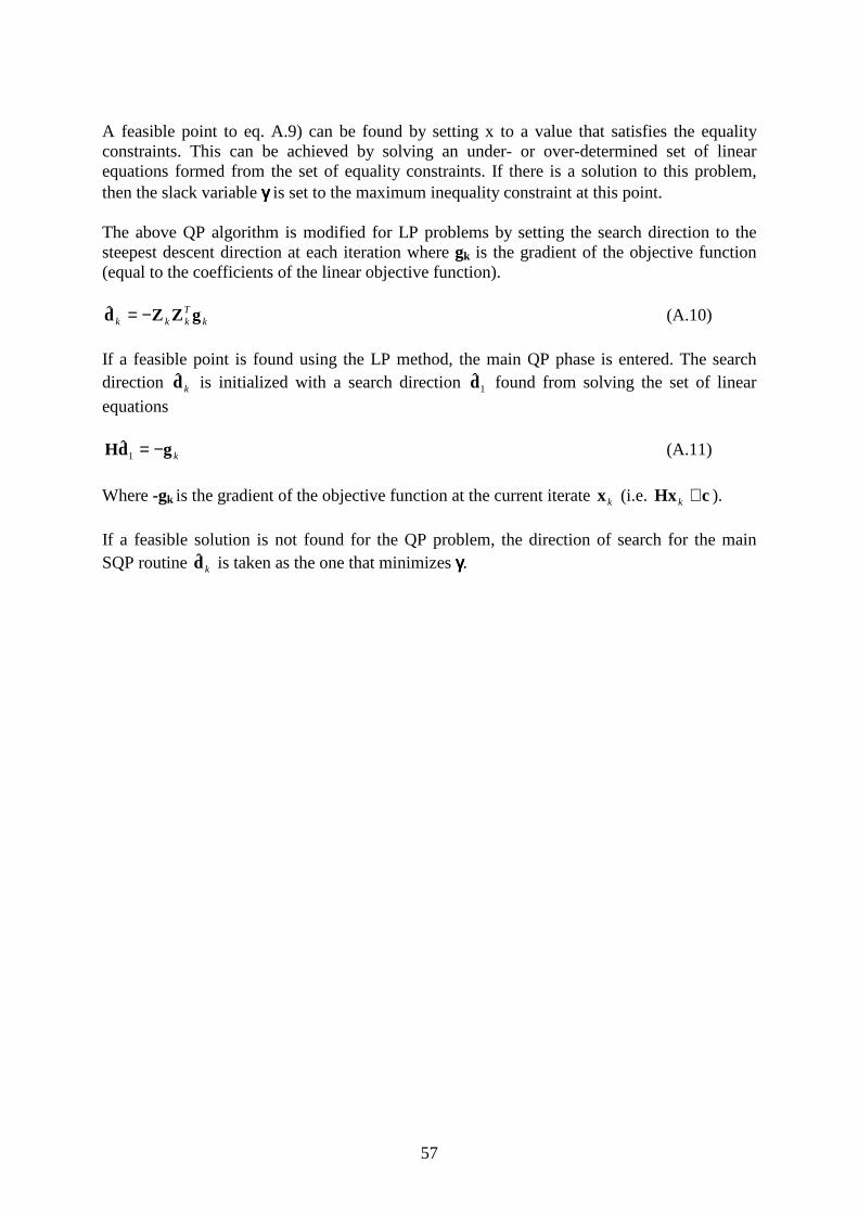
57

A feasible point to eq. A.9) can be found by setting x to a value that satisfies the equality constraints. This can be achieved by solving an under- or over-determined set of linear equations formed from the set of equality constraints. If there is a solution to this problem, then the slack variable γγγγ is set to the maximum inequality constraint at this point. The above QP algorithm is modified for LP problems by setting the search direction to the steepest descent direction at each iteration where gk is the gradient of the objective function (equal to the coefficients of the linear objective function).

kTkkk gZZd −=ˆ (A.10)

If a feasible point is found using the LP method, the main QP phase is entered. The search direction kd̂ is initialized with a search direction 1d̂ found from solving the set of linear

equations

kgdH −=1ˆ (A.11)

Where -gk is the gradient of the objective function at the current iterate kx (i.e. cHx +k ).

If a feasible solution is not found for the QP problem, the direction of search for the main SQP routine kd̂ is taken as the one that minimizes γγγγ.

58

Appendix B Creep test data Viscoelastic behavior is desbribed by creep compliance J(t) J(t) = strain developed in a creep test when loaded by a unit stress and relaxation modulus G(t) G(t) = stress developed in a relaxation test when loaded by a unit strain. Creep test data is given to Abaqus as the normalized shear and bulk compliances of the material. Js(t) = G0Js(t) and jk(t) = K0JK(t) (B.1) where Js(t) = 1/G(t) is the shear compliance, G0 =G(t = 0) is the instantaneous shear modulus, JK(t) = 1/K(t) is the bulk compliance and K0 = K(t = 0) is the instantaneous bulk modulus [abaqus standard users manual II]. This means that we have to transform the uniaxial creep test data into shear and bulk data.

Fig. B1. Creep test results. The creep modulus at an arbitrary time is

)()( 0

AAT t

tEεσ

= (B.2)

ε

59

Basic solid mechanics gives us the relation

GK

KGE

+=

3

9 (B.3)

If we assume that K is constant and E = E(t), B3 gives us

)(9

)(3)(

tEK

KtEtG

T

T

−= (B.4)

With B1, B2 and B4 we get the shear compliance

0

0

0

0 9

)(9

)()(

εσεσ

εε

−

−=

K

tK

ttj s (B.5)

The bulk modulus can be determined with uniaxial test data as

ν63−= E

K (B.6)

The creep test data are converted to relaxation data by Abaqus through the integral

� =−t

sR tdsstjsg0

)()( (B.7)

The normalized shear modulus gR(t) then is used in a non-linear least square fit to determine

the Prony series parameters P

ig−

and Giτ in the Prony series expansion

�=

−−

−−=N

i

ttP

iR

Giegtg

1

/ )1(1)( (B.8)

controlling the stress relaxation in the material[29].

MECHANICAL ANALYSIS OF A NONBRIDGING EXTERNAL FIXATION DEVICE · A NONBRIDGING EXTERNAL FIXATION...

Documents

Transcript of MECHANICAL ANALYSIS OF A NONBRIDGING EXTERNAL FIXATION DEVICE · A NONBRIDGING EXTERNAL FIXATION...