Measuring the Mutual Fund Industry Risk Management and...

Publisher: Asian Economic and Social Society ISSN: 2225-4226 Volume 3 No. 4 April 2013.

Measuring the Mutual Fund Industry Risk

Management and Performance Sustainability - Quantile

Regression Model

Joe-Ming Lee (Department of Banking and Finance, Tamkang

University, New Taipei City, Taiwan, ROC)

Citation: Joe-Ming Lee (2013). Measuring the Mutual Fund Industry Risk Management and

Performance Sustainability - Quantile Regression Model. Journal of Asian Business Strategy, Vol.

3, No. 4, pp. 59-68.

Measuring the Mutual Fund Industry ...

59

Author(s)

Joe-Ming Lee Department of Banking and Finance, Tamkang University,

New Taipei City, Taiwan, ROC

Measuring the Mutual Fund Industry Risk

Management and Performance Sustainability -

Quantile Regression Model

Abstract

We apply the Quantile Regression Model to observe the rank

correlation between bond fund performance and asset,

volatility, management fee, Sharpe index and show that fund

performance between volatility as a negative significant

relationship, implied extreme values have been generated risk

coefficient and fund performance change relations. The

extreme value of the display the risk coefficient fund

performance has changed the relationship, show that enhance

the risk coefficient, resulting in lower fund performance, tells

us that the mutual fund industry pursuit of short-term fund

performance through operating the transition risks lever, but

cannot afford a long-term test of the market. Finally, we

recommend that the mutual fund industry needs to strengthen

risk management professional and pursuit of performance

Sustainability.

Keywords: Equity fund, PSTR model, volatility, fund performance

Introduction

In light of the events of the past few years, the

environment in which mutual fund operate has

become significantly more “risk conscious”

and the question of what constitutes effective

“risk management” has become a key focus for

regulators, legislators and academics. Not

surprisingly, therefore, mutual fund seeks to

understand better their role in the risk

management process.

“Risk” is inherent in the investment

management business. In particular,

investment managers cannot invest their

clients’ funds and hope to earn a positive

return without taking some measure of risk. In

addition, in managing their businesses,

investment managers a wide variety of risks,

ranging from compliance-oriented risks to

reputational risks to risks to the systems they

use to run their businesses and beyond.

Because risk is at the core of the investment

management business, how investment

managers choose what risks to take and how

they monitor and manage those risks is

fundamental to their – and their clients’ –

success.

The Forum recognizes that the diversity among

funds and fund families and the constantly

evolving universe of risks in the market make

it impossible to develop a “one-size-fits-all”

approach to risk governance. Consequently,

directors should consider fund size, the assets

and number of funds in the fund family, the

Journal of Asian Business Strategy, 3(4): 59-68

60

structure of management and service

arrangements and fees, and the nature of fund

investment objectives and strategies, among

other factors, to determine whether and to what

extent particular principles are applicable and

appropriate.

In Taiwan, mutual funds are important

investment products. In particular, bond funds

are the largest types of mutual funds that the

managers of funds offer investors the

advantages of diversification and professional

assessment for risk on bonds and stocks

investment.

However, bond funds focus on pursuing short-

term high returns and increasing their scale by

investing in structured products with poor

liquidity. The problem arises when bond funds

allow clients to redeem and take their proceeds

the next day, engendering a liquidity

divergence between the bond funds’ own

assets and those offered to clients and

increasing the funds’ liquidity risks.

Although the local regulation for strengthening

bond fund management outlined major

management issues, the scarce liquidity

resulting from large holdings of structured

notes still triggered significant redemptions

upon Union Investment Trust and Tai-Yu

Investment Trust in Taiwan in July 2004. In

order to avoid risk, Taiwan’s Financial

Supervisory Commission (FSC) decided to

carry out a bond segregation policy before the

end of 2006. The system split up bond funds

into fixed income bond funds and quasi money

market bond funds.

Most studies in the bond fund literature focus

on funds’ performances, credit quality, and

value at risk (VaR). Some previous research

studies such as Blake, et al. (1993) used linear

and non-linear models to examine bond funds’

performances. Elton et al. (1995) first

developed and tested the relative pricing

models (based on the Arbitrage Pricing

Theory, or APT) to explain the expected

returns and performance of bond funds. These

two research studies concluded that active

funds do not outperform passive benchmarks.

Detzler (1999) evaluated the performance of

active global bond mutual funds and found no

support of superior fund performance net of

expenses against a wide range of benchmarks.

Some papers used Capital Asset Pricing Model

(CAPM) to evaluate the performance of bond

funds. Such as Gallagher and Jarnecic (2002)

who examined the investment performance of

active Australian bond funds and the impact of

investor fund flows on portfolio returns. Their

paper evaluated the performance of actively

managed Australian bond funds, using both

unconditional and conditional performance

evaluation techniques, and assessed the impact

of flow on retail bond fund performances.

Only Morey and O’Neal (2006) examined the

portfolio credit quality holding and daily return

patterns for bond mutual funds. They found

that bond funds on average hold significantly


61

more government bonds during disclosure than

during non-disclosure. Chen et al. (2010)

considered nine common factors and measured

the timing ability and performance of bond

mutual funds. They concluded that timing

ability generates non-linearity in fund returns

as a function of common factors, but there are

several non-timing-related sources of non-

linearity.

As mentioned above, we aim to look into the

effectiveness of mutual fund industry risk

management in Taiwan. Hence, the study

empirically investigates the effect of the risk

management through the ratio test, volatility

test, and Quantile Regression Model.

The remainder of the paper is organized as

follows. Section 2 takes a brief review of the

copula function. Section 3 provides our

empirical results. Section 4 is conclusion and

remarks.

Brief Review of the Quantile Regression

Model

We follow Shu et al. (2002) and use the panel

data model to estimate the mutual fund

performance, where the dependent variable is

monthly inflows, outflows, or net inflows of

each fund. To explain the relation between

fund performance relations, we use several

important variables as independent variables,

include, fund size (Asset), management fee

ratio (Fee), standard deviation of fund returns

(Volatility) and the Sharpe_ratio. The

regression model is as follows

Fund_Performancei,t = β0 + β1Asseti,t +

β2Feei,t+ β3Volatilityi,t+ β4Sharpe_indexi,t+ei,t

(1)

As with any mean-based procedure, the

ordinary regression model is sensitive to

outliers. Although outliers are occasionally

simply miscoded data, at other times missing

variables lead to extreme values for the error

terms. An obvious example in the case of

house price models is remodelling, which is

likely to produce an extremely high value for

the error terms when it is not observed in the

data set. The “quality” variable may also be

the source of outliers, Koenker and Bassett

(1978) originally proposed the quantile

regression approach.

Unlike ordinary least squares, the target for

quantile regression estimates is a parameter

that is specified before estimation. Let q

represent the target quantile. Also, let eit be the

residual implied by the econometric model.

Quantile parameter estimates are the

coefficients that minimize the following

objective function:

0 0

)1(22it ite e

itit eqeq (2)

At the median, q = 0.5, which implies that

equal weight is given to positive and negative


62

residuals. At the 90th

percentile, 2q = 1.8 and

2(1-q) = 0.2, which implies that more weight is

given to positive residuals – observations with

high values for the dependent variable, given

the values of the explanatory variables. This

result differs from ordinary least squares, in

which the sum of the residuals equals zero and

otherwise there is no constraint on the number

of positive residuals.

Each of these studies presents estimated

equations with the general form

qiuqi uxy . Quantile effects have a

straightforward missing variables inter-

pretation that follows directly from the hedonic

and repeat sales price index estimators.

Empirical Result Analysis

The dataset consists of bond funds that were

issued in Taiwan. For the purpose of

comparison, the sample period for the study

covers ten years, from January 2001 to June

2010. Table 1 presents a total of 32 bond

funds’ name, their trading code, and their

initiation date. The data were obtained from

the Taiwan Economic Journal (TEJ) database.

Table 1: Basic descriptions of the bond funds

Code Name of Bond Fund Initiation

Date Code Name of Bond Fund

Initiation

Date

UI02 Union Bond 1999/9/30 DF02 The Forever Bond Fund 1996/10/15

TR02 Manulife Wan Li

Bond Fund 1999/9/9 JF78

JF (Taiwan) First Bond

Fund 1996/10/15

BR02 Primasia Paoyen

Bond 1999/9/7 TS06 Shinkong Chi-Shin Fund 1996/9/3

TC18 IBT 1699 Bond Fund 1999/6/7 FP07 Fubon Chi-Hsiang Bond

Fund 1996/6/14

CP12 PCA Well Pool Fund 1998/12/23 CA02 Capital Safe Income

Bond Fund 1996/5/18

AP02 Manulife Wan Li

Bond Fund 1998/11/5 ML04

Prudential Financial

Bond Fund 1996/5/17

DS02 Truswell Bond Fund 1998/10/28 YC03 Hua Nan Phoenix Bond

Fund 1996/2/6

AI03 PineBridge Taiwan

Giant Fund 1998/9/7 CS03

Invesco ROC Bond

Fund 1995/11/9

TC02 IBT Ta-Chong Bond

Fund 1998/6/22 CI08

HSBC NTD Money

Management Fund 1995/11/2

GC02 SinoPac Bond Fund 1998/6/19 IC27 ING Taiwan Bond Fund 1995/10/21

FH02 Fuh-Hwa Bond Fund 1998/5/28 KY02 Polaris De-Li Bond

Fund 1995/9/21

JS02 Jih Sun Bond Fund 1997/10/3 PS04 UPAMC James Bond

Fund 1995/6/16

NC10 NITC Taiwan Bond

Fund 1997/3/7 JF75 JF Taiwan Bond 1995/6/15

YT08 Yuanta Wan-Tai

Bond Fund 1997/2/19 NC06 NITC Bond 1994/4/12


63

TI03 TIIM Bond Fund 1997/2/13 TS01 ShinKong High Yield 1994/1/31

CI10 HSBC NTD Money

Management Fund 2 1996/10/17 0008

ING Taiwan Income

Fund 1991/12/6

Note: The code represents the bond fund’s trading code, respectively.

As described above, this article investigates

the effect of a bond segregation policy in

Taiwan. The dataset hence consists of bond

funds that were issued in Taiwan. For the

purpose of comparison, the sample period for

the study covers ten years, from January 2001

to June 2010, total of 32 bond funds. The data

were obtained from the Taiwan Economic

Journal (TEJ) database.

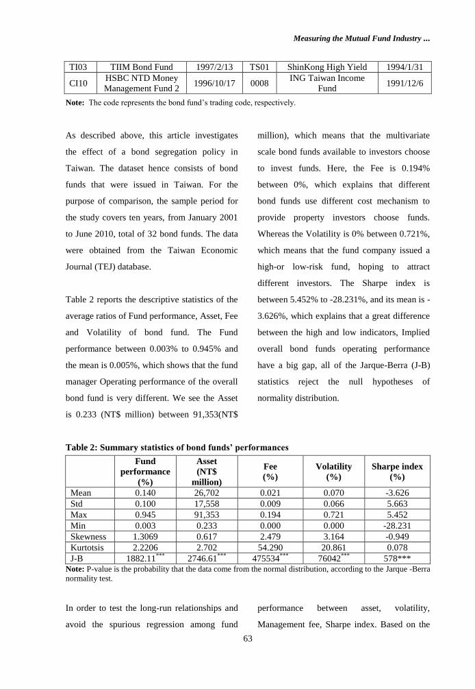
Table 2 reports the descriptive statistics of the

average ratios of Fund performance, Asset, Fee

and Volatility of bond fund. The Fund

performance between 0.003% to 0.945% and

the mean is 0.005%, which shows that the fund

manager Operating performance of the overall

bond fund is very different. We see the Asset

is 0.233 (NT$ million) between 91,353(NT$

million), which means that the multivariate

scale bond funds available to investors choose

to invest funds. Here, the Fee is 0.194%

between 0%, which explains that different

bond funds use different cost mechanism to

provide property investors choose funds.

Whereas the Volatility is 0% between 0.721%,

which means that the fund company issued a

high-or low-risk fund, hoping to attract

different investors. The Sharpe index is

between 5.452% to -28.231%, and its mean is -

3.626%, which explains that a great difference

between the high and low indicators, Implied

overall bond funds operating performance

have a big gap, all of the Jarque-Berra (J-B)

statistics reject the null hypotheses of

normality distribution.

Table 2: Summary statistics of bond funds’ performances

Fund

performance

(%)

Asset

(NT$

million)

Fee

(%)

Volatility

(%)

Sharpe index

(%)

Mean 0.140 26,702 0.021 0.070 -3.626

Std 0.100 17,558 0.009 0.066 5.663

Max 0.945 91,353 0.194 0.721 5.452

Min 0.003 0.233 0.000 0.000 -28.231

Skewness 1.3069 0.617 2.479 3.164 -0.949

Kurtotsis 2.2206 2.702 54.290 20.861 0.078

J-B 1882.11***

2746.61***

475534***

76042***

578*** Note: P-value is the probability that the data come from the normal distribution, according to the Jarque -Berra

normality test.

In order to test the long-run relationships and

avoid the spurious regression among fund

performance between asset, volatility,

Management fee, Sharpe index. Based on the


64

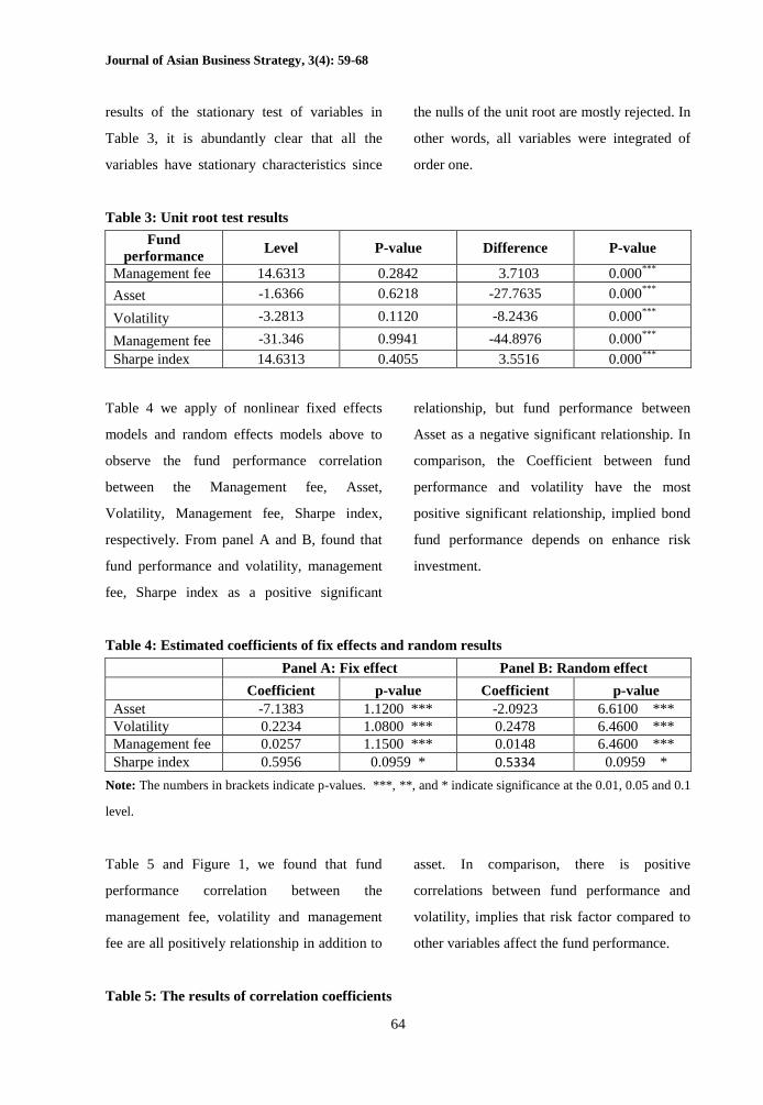
results of the stationary test of variables in

Table 3, it is abundantly clear that all the

variables have stationary characteristics since

the nulls of the unit root are mostly rejected. In

other words, all variables were integrated of

order one.

Table 3: Unit root test results

Fund

performance Level P-value Difference P-value

Management fee 14.6313 0.2842 3.7103 0.000***

Asset -1.6366 0.6218 -27.7635 0.000***

Volatility -3.2813 0.1120 -8.2436 0.000***

Management fee -31.346 0.9941 -44.8976 0.000***

Sharpe index 14.6313 0.4055 3.5516 0.000***

Table 4 we apply of nonlinear fixed effects

models and random effects models above to

observe the fund performance correlation

between the Management fee, Asset,

Volatility, Management fee, Sharpe index,

respectively. From panel A and B, found that

fund performance and volatility, management

fee, Sharpe index as a positive significant

relationship, but fund performance between

Asset as a negative significant relationship. In

comparison, the Coefficient between fund

performance and volatility have the most

positive significant relationship, implied bond

fund performance depends on enhance risk

investment.

Table 4: Estimated coefficients of fix effects and random results

Panel A: Fix effect Panel B: Random effect

Coefficient p-value Coefficient p-value

Asset -7.1383 1.1200 *** -2.0923 6.6100 ***

Volatility 0.2234 1.0800 *** 0.2478 6.4600 ***

Management fee 0.0257 1.1500 *** 0.0148 6.4600 ***

Sharpe index 0.5956 0.0959 * 0.5334 0.0959 *

Note: The numbers in brackets indicate p-values. ***, **, and * indicate significance at the 0.01, 0.05 and 0.1

level.

Table 5 and Figure 1, we found that fund

performance correlation between the

management fee, volatility and management

fee are all positively relationship in addition to

asset. In comparison, there is positive

correlations between fund performance and

volatility, implies that risk factor compared to

other variables affect the fund performance.

Table 5: The results of correlation coefficients


65

Fund

performance Asset std

Sharp

Index

Management

fee

1.0000 -0.2330 0.2564 0.1719 0.0543 Fund

performance

1.0000 -0.0604 0.3613 0.0036 asset

1.0000 0.2676 -0.0107 std

1.0000 0.0943 Sharpe Index

1.0000 management_fee

Figure 1: Fund performance versus volatility _all of bond funds

Table 6 reports a series of data can often

contain a structural break, due to a change in

policy or sudden shock to the economy. In

order to test for a structural break, we use the

Chow test, this is Chow’ first test (the second

test relates to predictions). The model in effect

uses an F-test to determine whether a single

regression is more efficient than two separate

regressions involving splitting the data into

two sub-samples.

We applied Chow test to formally test the

structural change of fund performance during

the period from January 2001 to June 2010.

The results of chow test show that the trend of

volatility of management fee significantly

existed structure-break which peak on

December 2005. It represents significant at 5%

significance level through Chow test on Table

6. Especially bond funds necessary for the

segregation policy was completed in

December 2005, a great shock result in bond

funds, fund changes in the market, because

investors fear generated for bond funds lost

confidence.

0

0.1

0.2

0.3

0.4

0.5

0.6

0.7

0.8

0.9

1

1 3 5 7 9 11 13 15 17 19 21 23 25 27 29

time series by group

Fund_performanc

Volatility


66

Table 6: The results of chow test

Chow statistics Breakpoint:2005/12 P-value

F(5, 110) 57.7918 0.0000***

F(9, 110) 422.2407 0.0000***

Note: *** denotes significant at the 1% significance level.

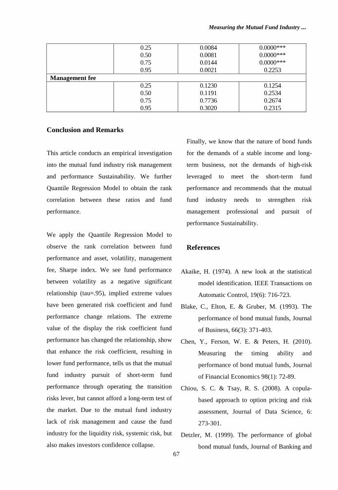
Table 7 we also apply the Quantile Regression

Model to observe the rank correlation between

fund performance and asset, volatility,

management fee, Sharpe index. We see the

fund performance and asset as a negative

significant relationship, volatility, fund

performance and volatility, Sharpe index as a

positive significant relationship (tau = 0.05,

0.25 0.50 0.75), but fund performance between

volatility as a negative significant relationship

(tau = 0.95), implied extreme values have been

generated risk coefficient and fund

performance change relations.

The extreme value of the display the risk

coefficient fund performance has changed the

relationship, said to enhance the risk

coefficient, resulting in lower fund

performance, tells us that the mutual fund

industry operating the transition risks lever, the

pursuit of short-term fund performance, but

cannot afford a long-term test of the market.

Due to the mutual fund industry and cause the

fund industry for the lack of risk management

of liquidity risk, systemic risk, but also makes

investors confidence collapse. We know that

the nature of bond funds for the demands of a

stable income and long-term business, not the

demands of high-risk leveraged to meet the

short-term fund performance, therefore, the

mutual fund industry needs to strengthen risk

management professional.

Table 7: Quantile regression model results

tau = 0.25, 0.50, 0.75, 0.95

Tau Coefficient P-value

Asset

0.25

0.50

0.75

0.95

-1.9051

-3.6469

-3.7863

-2.3510

0.0000***

0.0000***

0.0000***

0.0000*** Volatility

0.25

0.50

0.75

0.95

0.4413

0.5749

0.3378

-0.3393

0.0000***

0.0000***

0.0000***

0.0000***

Sharpe Index


67

0.25

0.50

0.75

0.95

0.0084

0.0081

0.0144

0.0021

0.0000***

0.0000***

0.0000***

0.2253

Management fee

0.25

0.50

0.75

0.95

0.1230

0.1191

0.7736

0.3020

0.1254

0.2534

0.2674

0.2315

Conclusion and Remarks

This article conducts an empirical investigation

into the mutual fund industry risk management

and performance Sustainability. We further

Quantile Regression Model to obtain the rank

correlation between these ratios and fund

performance.

We apply the Quantile Regression Model to

observe the rank correlation between fund

performance and asset, volatility, management

fee, Sharpe index. We see fund performance

between volatility as a negative significant

relationship (tau=.95), implied extreme values

have been generated risk coefficient and fund

performance change relations. The extreme

value of the display the risk coefficient fund

performance has changed the relationship, show

that enhance the risk coefficient, resulting in

lower fund performance, tells us that the mutual

fund industry pursuit of short-term fund

performance through operating the transition

risks lever, but cannot afford a long-term test of

the market. Due to the mutual fund industry

lack of risk management and cause the fund

industry for the liquidity risk, systemic risk, but

also makes investors confidence collapse.

Finally, we know that the nature of bond funds

for the demands of a stable income and long-

term business, not the demands of high-risk

leveraged to meet the short-term fund

performance and recommends that the mutual

fund industry needs to strengthen risk

management professional and pursuit of

performance Sustainability.

References

Akaike, H. (1974). A new look at the statistical

model identification. IEEE Transactions on

Automatic Control, 19(6): 716-723.

Blake, C., Elton, E. & Gruber, M. (1993). The

performance of bond mutual funds, Journal

of Business, 66(3): 371-403.

Chen, Y., Ferson, W. E. & Peters, H. (2010).

Measuring the timing ability and

performance of bond mutual funds, Journal

of Financial Economics 98(1): 72-89.

Chiou, S. C. & Tsay, R. S. (2008). A copula-

based approach to option pricing and risk

assessment, Journal of Data Science, 6:

273-301.

Detzler, M. (1999). The performance of global

bond mutual funds, Journal of Banking and


68

Finance, 23, 1195-1217.

Elton, E. J., Gruber, M. J. & Blake, C. R. (1995).

Fundamental economic variables, expected

returns, and bond fund performance,

Journal of Finance, 50(4): 1229-1256.

Gallagher, D. R. & Jarnecic, E. (2002). The

Performance of active Australian bond

funds, Australian Journal of Management,

27(2): 163-185.

Hsu, C. C., Tseng, C. P. & Wang, Y. H. (2008).

Dynamic hedging with futures: a copula-

based GARCH model. Journal of Futures

Markets, 28: 1095-1116.

Hu, L. (2006). Dependence patterns across

financial markets: a mixed copula

approach. Applied Financial Economics,

16(10): 717-729.

Hull, J. (2010). Risk management and financial

institutions, 2nd Edition, Pearson Prentice

Hall.

Joe, H. (1997). Multivariate models and

dependence concepts, London: Chapman &

Hall.

Junker, M., Szimayer, A. & Wagner, N. (2006).

Nonlinear term structure dependence:

copula functions, empirics, and risk

implications. Journal of Banking and

Finance, 30: 1171-1199.

Koenker, Roger & Gilbert, W. Bassett (1978).

Regression Quantiles, Econometrica, 46:

33-50.

Morey, M. R. & Neal, E. S. (2006). Window

dressing in bond mutual funds. Journal of

Financial Research, 29(3): 325-347.

Manner, H. & Reznikova, O. (2009). Time-

varying copulas: a survey, Universite

catholique de Louvain, Institut de

statistique, Mark, W. R., James, D. P.,

Paul, A. P. & Fran, X. (2001). Selecting a

bond mutual fund: just keep it simple.

Journal of Financial Planning, 14(4): 44-

49.

Nelsen, R. B. (2006). Introduction to copulas,

Springer Verlag, New York. 2nd Edition.

Palmon, O. & Jeffrey, P. (1991). Inflation

uncertainty, real interest rate uncertainty

and the liquidity premium on government

bonds. The Financial Review, 26: 459-477.

Palaro, H. P. & Hotta, L. K. (2006). Using

conditional copula to estimate value at risk,

Journal of Data Science, 4: 93-115.

Rodriguez, J. C. (2007). Measuring financial

contagion: a copula approach. Journal of

Empirical Finance, 14(3): 401-423.

Schwarz, G. (1978). Estimating the dimension of

a model. Annals of Statistics, 6: 461-464.

Shu, P. G., Yeh, Y. H. & Yamada, T. (2002). The

behavior of Taiwan mutual fund

investors—performance and fund flows.

Pacific-Basin Finance Journal, 10: 583–

600.

Sklar, A. (1959). Fonctions de repartition a n

dimensions et leurs marges.

Measuring the Mutual Fund Industry Risk Management and...

Documents

Transcript of Measuring the Mutual Fund Industry Risk Management and...