MEASURING THE EFFECTS OF MOBILITY ON REACTIVE … · MEASURING THE EFFECTS OF MOBILITY ON REACTIVE...

Helsinki University of Technology Laboratory for Theoretical Computer Science

Research Reports 91

Teknillisen korkeakoulun tietojenkasittelyteorian laboratorion tutkimusraportti 91

Espoo 2004 HUT-TCS-A91

MEASURING THE EFFECTS OF MOBILITY ON REACTIVE AD

HOC ROUTING PROTOCOLS

Mikko Sarela

AB TEKNILLINEN KORKEAKOULUTEKNISKA HÖGSKOLANHELSINKI UNIVERSITY OF TECHNOLOGYTECHNISCHE UNIVERSITÄT HELSINKIUNIVERSITE DE TECHNOLOGIE D’HELSINKI

Helsinki University of Technology Laboratory for Theoretical Computer Science

Research Reports 91

Teknillisen korkeakoulun tietojenkasittelyteorian laboratorion tutkimusraportti 91

Espoo 2004 HUT-TCS-A91

MEASURING THE EFFECTS OF MOBILITY ON REACTIVE AD

HOC ROUTING PROTOCOLS

Mikko Sarela

Helsinki University of Technology

Department of Computer Science and Engineering

Laboratory for Theoretical Computer Science

Teknillinen korkeakoulu

Tietotekniikan osasto

Tietojenkasittelyteorian laboratorio

Distribution:

Helsinki University of Technology

Laboratory for Theoretical Computer Science

P.O.Box 5400

FIN-02015 HUT

Tel. +358-0-451 1

Fax. +358-0-451 3369

E-mail: [email protected]

©c Mikko Sarela

ISBN 951-22-7145-1

ISSN 1457-7615

Multiprint Oy

Helsinki 2004

ABSTRACT: Ad hoc networks can operate without fixed infrastructure andcan survive rapid changes in the network topology. They can be studiedformally as graphs in which the set of edges varies in time.

The main method for testing ad hoc networks is simulation. Choosing mo-bility model that describes the movements of the nodes in statistical terms isone of the most important choices of simulation parameters. This is becausethe location of nodes determines whether any pair of nodes has a direct com-munication link and the location of each node is determined by movement.

These links are used for creating routes between nodes that are not ad-jacent. When a link that is part of a route goes down, the route has to berebuilt, which causes delays, packet loss and routing protocol overhead inthe network. This report proposes that the route life time can be used as anindicator of the effects of mobility for reactive ad hoc routing. A method forestimating the route life time distribution for shortest routes between randomnodes is also proposed.

The simulations do not correspond with the predictions of the model. Thismeans that the model is lacking some critical aspect. Further research isrequired to understand the factors that affect reactive ad hoc routing protocolperformance.

KEYWORDS: ad hoc network, routing, mobility management, mobility model,simulation

Contents

1 Introduction 1

2 Mobile Ad Hoc Networking 32.1 Ad Hoc Routing Protocols . . . . . . . . . . . . . . . . . . . 3

AODV . . . . . . . . . . . . . . . . . . . . . . . . . . . . . . 3DSR . . . . . . . . . . . . . . . . . . . . . . . . . . . . . . . 4

2.2 Modeling Ad Hoc Networks . . . . . . . . . . . . . . . . . . 4

2.3 Simulation . . . . . . . . . . . . . . . . . . . . . . . . . . . 42.4 Mobility Models . . . . . . . . . . . . . . . . . . . . . . . . 42.5 Problem Statement . . . . . . . . . . . . . . . . . . . . . . . 5

3 Design Criteria 63.1 Clarity . . . . . . . . . . . . . . . . . . . . . . . . . . . . . . 63.2 Predictivity . . . . . . . . . . . . . . . . . . . . . . . . . . . 63.3 Consistence . . . . . . . . . . . . . . . . . . . . . . . . . . . 6

4 Previous Work 74.1 Graph Theory . . . . . . . . . . . . . . . . . . . . . . . . . . 74.2 Suggested Models for Effects of Mobility on Ad Hoc Routing 7

Early Models on the Effects of Mobility . . . . . . . . . . . . 8Effects of Mobility Come to Focus . . . . . . . . . . . . . . . 8Mobility Analysis Matures . . . . . . . . . . . . . . . . . . . 9

Summary . . . . . . . . . . . . . . . . . . . . . . . . . . . . 114.3 Mobility Models . . . . . . . . . . . . . . . . . . . . . . . . 114.4 Other Mobility Models . . . . . . . . . . . . . . . . . . . . . 14

Entity Models . . . . . . . . . . . . . . . . . . . . . . . . . . 14Group Mobility Models . . . . . . . . . . . . . . . . . . . . 17Individually Simulated Mobility Model . . . . . . . . . . . . 18

4.5 Simulators . . . . . . . . . . . . . . . . . . . . . . . . . . . . 18

5 Measuring Mobility 205.1 Dynamic Networks . . . . . . . . . . . . . . . . . . . . . . . 205.2 Distance Distribution . . . . . . . . . . . . . . . . . . . . . . 205.3 Measuring Remaining Link Life Time Distribution . . . . . . 215.4 Route Life Time Distribution (rlt) . . . . . . . . . . . . . . . 21

Average Route Life Time . . . . . . . . . . . . . . . . . . . . 22Percentile of Route Life Time . . . . . . . . . . . . . . . . . 22

Percentage of Routes Valid After t Seconds . . . . . . . . . . 22Proposed Variant . . . . . . . . . . . . . . . . . . . . . . . . 23

6 Simulations 246.1 Finding Route Life Time Distribution . . . . . . . . . . . . . 256.2 Simulation Results for Testing Hypothesis . . . . . . . . . . . 25

Mobility Pattern . . . . . . . . . . . . . . . . . . . . . . . . . 26

7 Simulation Results 27

iv CONTENTS

8 Analysis 338.1 Simulation Analysis . . . . . . . . . . . . . . . . . . . . . . . 33

Distance Distribution . . . . . . . . . . . . . . . . . . . . . . 33Link Life Time Distribution . . . . . . . . . . . . . . . . . . 34Route Life Time Distribution . . . . . . . . . . . . . . . . . 34

8.2 Criterion Analysis . . . . . . . . . . . . . . . . . . . . . . . . 35Clarity . . . . . . . . . . . . . . . . . . . . . . . . . . . . . . 35Predictivity . . . . . . . . . . . . . . . . . . . . . . . . . . . 35Consistency . . . . . . . . . . . . . . . . . . . . . . . . . . . 36

8.3 Summary . . . . . . . . . . . . . . . . . . . . . . . . . . . . 38

9 Conclusions 41

Acknowledgements 43

References 47

A Distance Distribution 48

B Link Life Time Distribution 51

C Route Life Time Distribution Distribution 56

CONTENTS v

List of Figures

1 Random walk mobility pattern . . . . . . . . . . . . . . . . . 122 Random direction mobility pattern . . . . . . . . . . . . . . . 123 Gauss-Markov mobility pattern . . . . . . . . . . . . . . . . . 134 Random waypoint mobility pattern . . . . . . . . . . . . . . . 145 Boundless simulation area mobility pattern . . . . . . . . . . 156 Probabilistic version of random walk mobility pattern . . . . . 167 The link lifetime distribution for Random Walk in Scenarios

1, 2,3 and 3 . . . . . . . . . . . . . . . . . . . . . . . . . . . 278 The link lifetime distribution for Random Direction in Sce-

narios 1, 2, and 3 . . . . . . . . . . . . . . . . . . . . . . . . 289 The link lifetime distribution for Gauss-Markov in Scenarios

1, 2, and 3 . . . . . . . . . . . . . . . . . . . . . . . . . . . . 2910 The route lifetime distribution for Random Walk in Scenar-

ios 1, 2, and 3 . . . . . . . . . . . . . . . . . . . . . . . . . . 3011 The route lifetime distribution for Random Direction in Sce-

narios 1, 2, and 3 . . . . . . . . . . . . . . . . . . . . . . . . 3112 The route lifetime distribution for Gauss-Markov in Scenar-

ios 1, 2, and 3 . . . . . . . . . . . . . . . . . . . . . . . . . . 3113 The link lifetime distribution for Random Walk in Scenario 1 5114 The link lifetime distribution for Random Walk in Scenario 2 5115 The link lifetime distribution for Random Walk in Scenario 3 5216 The link lifetime distribution for Random Direction in Sce-

nario 1 . . . . . . . . . . . . . . . . . . . . . . . . . . . . . . 5217 The link lifetime distribution for Random Direction in Sce-

nario 2 . . . . . . . . . . . . . . . . . . . . . . . . . . . . . . 5318 The link lifetime distribution for Random Direction in Sce-

nario 3 . . . . . . . . . . . . . . . . . . . . . . . . . . . . . . 5319 The link lifetime distribution for Gauss-Markov in Scenario 1 5420 The link lifetime distribution for Gauss-Markov in Scenario 2 5421 The link lifetime distribution for Gauss-Markov in Scenario 3 5522 The route lifetime distribution for Random Walk in Scenario 1 5623 The route lifetime distribution for Random Walk in Scenario 2 5624 The route lifetime distribution for Random Walk in Scenario 3 5725 The route lifetime distribution for Random Direction in Sce-

nario 1 . . . . . . . . . . . . . . . . . . . . . . . . . . . . . . 5726 The route lifetime distribution for Random Direction in Sce-

nario 2 . . . . . . . . . . . . . . . . . . . . . . . . . . . . . . 5827 The route lifetime distribution for Random Direction in Sce-

nario 3 . . . . . . . . . . . . . . . . . . . . . . . . . . . . . . 5828 The route lifetime distribution for Gauss-Markov in Scenario 1 5929 The route lifetime distribution for Gauss-Markov in Scenario 2 5930 The route lifetime distribution for Gauss-Markov in Scenario 3 60

vi LIST OF FIGURES

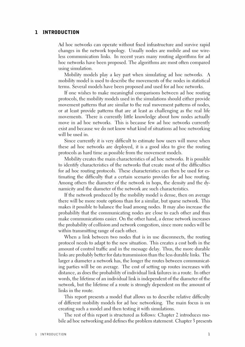
1 INTRODUCTION

Ad hoc networks can operate without fixed infrastructure and survive rapidchanges in the network topology. Usually nodes are mobile and use wire-less communication links. In recent years many routing algorithms for adhoc networks have been proposed. The algorithms are most often comparedusing simulation.

Mobility models play a key part when simulating ad hoc networks. Amobility model is used to describe the movements of the nodes in statisticalterms. Several models have been proposed and used for ad hoc networks.

If one wishes to make meaningful comparisons between ad hoc routingprotocols, the mobility models used in the simulations should either providemovement patterns that are similar to the real movement patterns of nodes,or at least provide patterns that are at least as challenging as the real lifemovements. There is currently little knowledge about how nodes actuallymove in ad hoc networks. This is because few ad hoc networks currentlyexist and because we do not know what kind of situations ad hoc networkingwill be used in.

Since currently it is very difficult to estimate how users will move whenthese ad hoc networks are deployed, it is a good idea to give the routingprotocols as hard time as possible from the movement models.

Mobility creates the main characteristics of ad hoc networks. It is possibleto identify characteristics of the networks that create most of the difficultiesfor ad hoc routing protocols. These characteristics can then be used for es-timating the difficulty that a certain scenario provides for ad hoc routing.Among others the diameter of the network in hops, the density and the dy-namicity and the diameter of the network are such characteristics.

If the network produced by the mobility model is dense, then on averagethere will be more route options than for a similar, but sparse network. Thismakes it possible to balance the load among nodes. It may also increase theprobability that the communicating nodes are close to each other and thusmake communications easier. On the other hand, a dense network increasesthe probability of collision and network congestion, since more nodes will bewithin transmitting range of each other.

When a link between two nodes that is in use disconnects, the routingprotocol needs to adapt to the new situation. This creates a cost both in theamount of control traffic and in the message delay. Thus, the more durablelinks are probably better for data transmission than the less durable links. Thelarger a diameter a network has, the longer the routes between communicat-ing parties will be on average. The cost of setting up routes increases withdistance, as does the probability of individual link failures in a route. In otherwords, the lifetime of an individual link is independent of the diameter of thenetwork, but the lifetime of a route is strongly dependent on the amount oflinks in the route.

This report presents a model that allows us to describe relative difficultyof different mobility models for ad hoc networking. The main focus is oncreating such a model and then testing it with simulations.

The rest of this report is structured as follows: Chapter 2 introduces mo-bile ad hoc networking and defines the problem statement. Chapter 3 presents

1 INTRODUCTION 1

the criteria that the given model will be tested against. Most relevant previ-ous work on this field is explained in Chapter 4. The proposed model isexplained in Chapter 5. Chapter 6 explains the simulations done to test themodel and Chapter 7 contains the simulation results. Chapter 8 containsthe analysis of the proposed model. Chapter 9 concludes the report andgives ideas for future work on subject.

2 1 INTRODUCTION

2 MOBILE AD HOC NETWORKING

Traditionally communication networks have been static, or nearly static. Whencomputing devices became smaller and portable, need for solving mobilityproblems arouse. There are multiple different solutions that enable individ-ual nodes to change their location in the network, but the main paradigm ofstatic network infrastructure still remains.

However, there are many communication problems that prohibit the ex-istence of static infrastructure. The most researched such areas have beenmilitary communications and disaster recovery. To solve these problems, anew dynamic network structure paradigm, ad hoc networks was created [29].

An ad hoc network consists of nodes that communicate with each otherwithout the help of pre-existing infrastructure. The links between the nodesmay change and the network adapts rapidly to the new situation. The chang-ing network topology is usually due to mobile nodes using wireless links, butthe techniques that solve the problems are not limited to such an arrange-ment.

The first problem in dynamic networks is delivering the information to itsrecipient. There are many different ad hoc routing protocols that tackle thisproblem (e.g. [7, 10, 12, 17, 20, 22, 25, 28, 30, 37, 39, 40, 41, 42, 46]).

2.1 Ad Hoc Routing Protocols

Ad hoc routing protocols can be divided into categories based on how theyoperate. Some protocols maintain topology information all the time [42]and some quickly find out the topology, information, or route to destination,only when that information is needed, i.e. on-demand [28, 41]. These arecalled proactive and reactive protocols, respectively. Some protocols con-sider all nodes equal and flat topology [28, 41, 42], where as some protocolsuse clusters or more complicated hierarchies to manage to dynamic network[10, 22, 25, 30, 40].

AODV

AODV [41] is the Ad-hoc On-Demand Distance Vector routing protocol.It is reactive by its nature and AODV nodes gather information relevant torouting from their surroundings only when it is needed.

When a node wishes to communicate to another, it broadcasts a route re-quest (RREQ). This request is flooded throughout the network until a nodewith a valid route to the destination is found. Flooding means that the initia-tor and each node that receives it broadcasts the packet to all its neighbors,ensuring the message is received by all reachable nodes.The node with valid route to the destination then sends a route reply (RREP)back to the original sender using the route through which it received theRREQ. Each node stores information about the RREQ into its routing table.This information is stored only for a short period of time, unless the nodebecomes part of the route between the source and the destination.

2 MOBILE AD HOC NETWORKING 3

DSR

DSR [28] is a dynamic source routing protocol. As its name says, it usessource routing principle. That is, when a node sends a packet to anothernode, it attaches to the packet the exact route with which the packet must beforwarded.

If the sender does not know the exact route to the recipient, it will discoverthe route using a route discovery protocol. A packet requesting a route to thedestination is flooded through out the network. The first receiver to know aroute will send back a message with the full route to the destination.

2.2 Modeling Ad Hoc Networks

There are three different ways to model networks: formal analysis, real lifemeasurements and simulation. The dynamic nature of ad hoc networksmakes them hard to study by formal analysis.

Some formal techniques that have been used in static networks includePetri nets, stochastic processes, queuing theory, and graph theory. None ofthese is especially well suited to studying dynamic networks.

Since ad hoc networks are still mainly a research subject, most scenariosthey will be used in are still unknown. For those scenarios that are known,e.g. military networks, extreme uncertainties and dynamicity are expected.Thus use of real life measurements is currently almost impossible and cer-tainly costly. The commonly used alternative is study the behavior of theprotocols in a simulated environment.

2.3 Simulation

The purpose of simulation is to create an artificial environment, usually acomputer program, that captures the essential characteristics of the phenom-ena that is begin studied. Using simulations is cheap, which makes it eco-nomically viable possible to create a statistically significant amount of testruns. For these reasons simulation is a much used tool for comparing ad hocrouting protocols.

There are several network simulators that can be used for studying mobilead hoc networks. [1, 2, 19, 38]

Ad hoc network researchers face the problem of not knowing how nodeswill operate in real life situations, especially, how they will move. In order tocreate meaningful simulation results, good understanding of mobility and itseffects on ad hoc routing is required.

2.4 Mobility Models

Mobility models are used to describe the movements of nodes statistically.Each model gives an algorithm that is used to randomize the movement ofnodes. Mobility pattern is the actual set of movements that result from apply-ing the mobility model to one, or more nodes. The models are divided intotwo categories, the entity mobility models and the group mobility models.

Entity mobility model gives a statistical movement description of a singlenode. This model can then be used to generate movements of several nodes

4 2 MOBILE AD HOC NETWORKING

by running the corresponding algorithm that generates the mobility patternseveral times. Section 4.3 describes several models in more detail.

Group mobility model randomizes the movement of nodes such that themovement of nodes in the same group are correlated. One typical way ofaccomplishing this is to have a group center for each group, which movesand then allow the node positions to vary around that point.

2.5 Problem Statement

The main objective of this report is to design an experimental method for ex-plaining the most significant impacts of mobility in wireless ad hoc networksthat use reactive routing protocols.

This work evaluates existing entity mobility models, namely random walk,random direction and Gauss-Markov. Existing reactive ad hoc routing proto-cols, i.e. AODV and DSR are used to verify the results.

2 MOBILE AD HOC NETWORKING 5

3 DESIGN CRITERIA

This section presents the criteria that the proposed method for explaining im-pact of mobility should meet. The proposed method must be in the form ofparameters that can be easily measured from the simulations. These param-eters should characterize the effects of mobility on reactive ad hoc routing.

3.1 Clarity

The proposed method will suggest a small number of mobility parametersthat constitute the most significant impact on reactive routing. These must besuch that a human can easily understand them and that a computer programcan be used for ranking different scenarios according to their relative effectof reactive ad hoc routing.

This means that the number of significant parameters must be small andif multiple characteristics are suggested, a way to norm these into one singlemust be presented.

3.2 Predictivity

The proposed method must provide predictions on simulation results andsimulation results done with actual reactive routing protocols must verifythem. These predictions will take the form that mobility model A with cer-tain mobility parameters will be harder, or easier for ad hoc routing thanmobility model B with certain parameters.

Two measurements, average packet throughput and packet overhead willbe used for measuring the hardness.

3.3 Consistence

The parameters that are found must have small variation from one simulationto another. This will be verified by comparing two sets of simulations withsame mobility parameters.

6 3 DESIGN CRITERIA

4 PREVIOUS WORK

There are two main problems for comparing the efficiency of ad hoc networkrouting protocols via simulation. We do not know how actual users moveand we do not know the communication patterns that users will effect on thenetwork.

Much research has been done to understand mobility in structured net-works, such as GSM networks. There are several different mobility modelsfor GSM networks and the effects of mobility has been analyzed in detail[4, 21, 23, 35, 36, 43, 44]. Zonoozi et al [51] have a good survey of existingmobility models and their analysis for GSM networks.

Unfortunately these models and analysis are not suitable for ad hoc net-works. GSM networks are based on cellular model, i.e. the physical geo-graphical area is divided into cells and each cell is dominated by one basestation. The problem in GSM networks is to understand how mobile nodesmove between these cells. This makes it accurate enough to use flow models,i.e. merely model the movement of nodes from each cell to its neighbours.

On the other hand, in ad hoc networks the connectivity is based on mo-bile nodes connecting to each other. This means that the distance betweeneach pair of nodes has to be known. Thus, the locations and movements ofnodes have to be modeled more precisely than those in GSM networks, forexample.

The rest of this chapter is organized as follows. First part will introducethe graph theoretic definitions required for the rest of the report. The nextpart explains how the effects of mobility on ad hoc networking have beenmeasured and quantified in earlier research. After that the most relevant mo-bility models and network simulators for ad hoc network simulation studiesare described.

4.1 Graph Theory

This report models ad hoc networks as graphs, where each link between anypair of nodes either exists or does not exist at any given moment of time. Thebasic definitions for graphs come from Diestel [15].

Graph is a pair of finite sets G = (V, E) that satisfies E ⊆ V × V .A pair (A, B) ∈ E is called a link.Path from A to B is a non-empty graph P = (V, E) such that V =

{x1, . . . , xk} and E = {(x1, x2); (x2, x3); . . . ; (xk−1, xk)} and x1 = A andxk = B. The length of the path is k − 1 and is denoted by |PA,B|.

The distance D between two nodes A ∈ V and B ∈ V for graph G is:(1) D = ∞ if no path exists between the nodes.

(2) D = min(|PA,B|, for all paths from A to B)

There are many algorithms for finding the shortest path between twonodes in a graph [11, 16].

4.2 Suggested Models for Effects of Mobility on Ad Hoc Routing

Interest in the effects of mobility on ad hoc networks has grown in the pastfew years. This section presents previous attempts to characterize the effects

4 PREVIOUS WORK 7

of mobility on ad hoc routing.

Early Models on the Effects of MobilityUntil late 90s little effort was put into understanding the effects of mobilityon ad hoc networking. The focus was clearly on creating new kinds of rout-ing protocols and comparing them. Less thought was put into understandinghow mobility affects routing. This is quite understandable, since it was moreimportant to be able to propose protocols with new qualities and better per-formance for different scenarios.

Broch et al [7] suggested that mobility could be characterized using thelength of time that nodes stay stationary between periods of movement. Thisapproach works quite well, when nodes spend most of their time still andmove only rarely. Unfortunately most models and scenarios do not consist ofnodes sitting around doing nothing most of the time. Thus this characteriza-tion fails to depict the true nature of mobility.

Camp [8] proposes average speed of the nodes for representing their mo-bility.

These models do not show an accurate picture, because they considerthe speeds of the nodes relative to the surroundings and not relative to othernodes. Thus the model fails to depict correctly the amount of dynamicitycaused by moving nodes.

Effects of Mobility Come to FocusAs ad hoc networks research has started to mature, interest in the effects ofmobility has risen. Some researchers started analyzing and creating bettermodels to study effects of mobility. Several papers which had emphasis onanalysis of mobility were written.

Larsson et. al [33] proposed a model of mobility for characterizing move-ment in ad hoc networks. The idea is to calculate a mobility metric calledmobility to characterize the difficulties that mobility creates for ad hoc rout-ing. Mobility measures the change in average distance (Ax) from one nodeto all other nodes between successive simulation time steps (∆t). This isthen averaged over the whole simulation time (T ) and all nodes. Equation 1shows the average mobility for one node through the simulation. The mobil-ity metric they propose is the average of this over all nodes.

Mx =

∑T−∆tt=0 |(Ax(t) − Ax(t + ∆t))

T − ∆t(1)

Johansson et. al [27] refined the model developed in [33]. Their model cal-culates the following metric. For each moment the relative velocity betweentwo nodes x and y is v(x, y, t). The mobility metric for the pair of nodes isthe absolute relative speed (v(x, y, t)) averaged over the simulation time (T )as shown in Equation 2. The mobility metric over the whole simulation isthe average of this over all node pairs.

Mxy =1

T

∫ T

0|v(x, y, t)| dt (2)

Their purpose was to show that this metric, which describes the velocity ofthe nodes relative to each other, is linearly correlated with amount of link

8 4 PREVIOUS WORK

changes. Kwak has proposed another model, which describes the amount oflink changes in terms of relative movement velocity [31, 32].

These proposals still suggest a single mobility metric, which should beable to quantify the effects of mobility on all different ad hoc routing proto-cols. For example reactive ad hoc routing is dependent on the life time ofthe used route, whereas proactive routing protocols are dependent on the lifetime of each individual link. This is because in reactive ad hoc routing, evena single failed link in a route causes packets to be dropped, or delayed andmuch extra overhead to restore the route. Similarly each link changes causespacket overhead in the network that is trying to adjust to the new situation.

Turgut et al [50] proposed that the expected lifetime of the route is theimportant metric. He also proposed that the lifetime of a route can be es-timated with the minimum of the expected lifetimes for all the hops. Thelatter claim doesn’t hold as shown in Chapter 5.

Mobility Analysis Matures

Currently, mobility research on ad hoc networks focuses in understandingdifferent parts of ad hoc routing protocols and the way these parts are af-fected by mobility. For example one can define a flooding building block.Flooding means that a packet is propagated from the sender to all receiversthat are within the radius of flooding. This method is commonly used in re-active routing protocols for finding a route to destination.This enables one to study the behavior of each generic building block indifferent mobility schemes and find out how and why mobility affects theperformance of the building block in question. For example one can studythe building block, e.g. flooding protocol in different mobility schemes andthen conclude that the analysis is valid for any protocol that uses flooding.This method was suggested by Bai et al [18]

Bai et al [3] also suggested several metrics for analyzing how mobility af-fects routing protocol performance. The studied metrics were divided intotwo different groups: Mobility metrics and connectivity graph metrics. Amongothers, average degree of spatial dependence and average relative speed, andaverage number of link changes and average link duration and average pathavailability were defined.Degree of spatial dependence for two nodes is defined as the cosine of theangle between their velocities multiplied by their speed ratio. Average spatialdependence is the average of the pairwise spatial dependence over all nodesthat are within a certain predetermined range. The relative speed RS of two

nodes i and j at time t is RS(i, j, t) =|→

Vi(t) −→

Vj(t)|

In the study they measured spatial dependence and average relative speedwith different range values to find out which range values could differentiatedifferent mobility scenarios they studied. In both the range value of twicethe transmission range could differentiate the scenarios clearly. The researchgroup also found indication that average relative speed metric is correlatedwith maximum velocity of the nodes.The average number of link changes did not seem to have an effect on simu-lation results [3]. This is easy to explain, since high number of link changes

4 PREVIOUS WORK 9

can either come from the scenario having a high amount of relatively stablelinks, or a relatively low amount of links with low lifetime. Since the metriccannot distinguish between those two situations, it does not provide usefulinformation.Bai et al [3] also notice that average link duration has a strong correlationwith routing protocol performance, which has been shown in previous stud-ies.They did not find average path availability to be a good metric. Average pathavailability describes the portion of time that a path is available from a cer-tain node to another averaged over all node pairs. This may be because theyused simulations in which it was rare for a node to be disconnected from anetwork.

Sadagopan et al [47] studied the probability density functions of link andpath lifetime. They define link lifetime to be the time that a link is con-tinuously up from the point of time when it becomes into existence to thepoint of time, when it dies. Their definition of path lifetime for path P =n1, n2, . . . , nk at time t is the longest continuous time interval during whichall k − 1 links exists. Thus path lifetime is constrained by the life time of thelink with shortest lifetime in the path.

In the same paper, the authors also suggest that the throughput of DSR[28] is dependent only on the portion of time used to transfer data and thetime used to repair broken paths. The overhead is dependent only on theaverage path duration, fraction of requests replied by first hop neighbors andnumber of nodes. The study proposed following equations:throughput = (1 − trepair

DP)r

overhead = TDP

(p · 1 + (1 − p)N), where

• N is the total number of nodes

• T is the total simulation time

• trepair is the time spent to repair a broken path each time

• DP is the average path duration

• r is the data rate, which is assumed to be constant

• p is the fraction of requests answered by first hop neighbors

In other words, the maximum throughput of the network cannnot be higherthan a certain percentage of the data rate in which the percentage is the frac-tion of time a valid route between two communicating parties exists. How-ever, this only applies to real time traffic. For non-real time traffic, the datarate r needs to be replaced with maximum bandwidth of the network.The overhead metric calculates the expected amount of control messages re-quired to keep one connection up for the duration of the simulation. Thefraction T

DPexpresses the expected amount of path breakages and the latter

portion of the equation the expected amount of control messages required torepair the path. The simulation results show high correlation for the averagepath duration and throughput and overhead (> 0.9) for Random Waypoint,Freeway and Manhattan mobility models, but not for Reference Point Group

10 4 PREVIOUS WORK

Mobility model. These models are described in Section 4.3.

Summary

In past few years, several different metrics have been proposed in order toquantify the effects of mobility on ad hoc networking. This is an ongoingwork just getting started. The metrics that currently seem most profitable arelink life time and route life time distributions.

It also seems clear that no one metric that can accurately describe theeffect of mobility on all ad hoc networks.

The building block approach [3, 18, 47] is the best framework that cur-rently exists to understand the effects of mobility on ad hoc networking.

4.3 Mobility Models

Ad hoc mobility models are used to describe the movements of nodes statis-tically. Each model gives an algorithm that is used to randomize the move-ment of nodes. The models are divided into two categories, entity mobilitymodels and group mobility models [13]. The entity mobility models ran-domize the movements of each individual node. The group mobility modelshave groups of nodes that stay close to each other and then randomize themovement of the group. The node positions also vary randomly around thegroup reference point.

This report examines only entity models, mainly because currently theyare most often used in simulations for ad hoc routing protocol comparisons.They are also chosen, because the mobility patterns they produce are simplerto analyze and thus provide a better starting point for the research.

This section presents the entity mobility models used in this report.

Random Walk Random walk is a simple mobility model. Each node movesin a straight line for a predetermined time t. The direction is picked at ran-dom from uniform distribution between 0 and 2π and the speed is randomlychosen from uniform distribution between Speedmin and Speedmax. Thenode then moves for a time t and then picks another direction and speedat random. The simulation parameters for random walk mobility models areshown in Table 1.

Table 1: Simulation Parameters for random walk

Speedmin Minimum SpeedSpeedmax Maximum Speedt Duration between changes of speed and direction

Random walk is a memoryless mobility model. It assumes that the behav-ior of the node does not depend in any way from its past history. Randomwalk is often referred to as brownian motion.

Figure 1 shows an example of one node moving in a 300 m × 300 m areausing random walk mobility model. As can be seen from the picture the node

4 PREVIOUS WORK 11

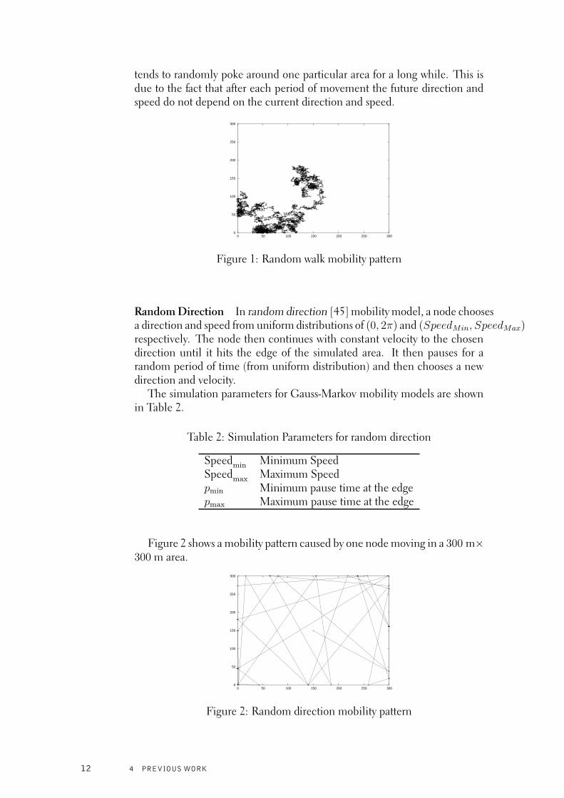
tends to randomly poke around one particular area for a long while. This isdue to the fact that after each period of movement the future direction andspeed do not depend on the current direction and speed.

0

50

100

150

200

250

300

0 50 100 150 200 250 300

Figure 1: Random walk mobility pattern

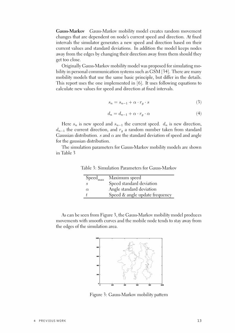
Random Direction In random direction [45] mobility model, a node choosesa direction and speed from uniform distributions of (0, 2π) and (SpeedMin, SpeedMax)respectively. The node then continues with constant velocity to the chosendirection until it hits the edge of the simulated area. It then pauses for arandom period of time (from uniform distribution) and then chooses a newdirection and velocity.

The simulation parameters for Gauss-Markov mobility models are shownin Table 2.

Table 2: Simulation Parameters for random direction

Speedmin Minimum SpeedSpeedmax Maximum Speedpmin Minimum pause time at the edgepmax Maximum pause time at the edge

Figure 2 shows a mobility pattern caused by one node moving in a 300 m×300 m area.

0

50

100

150

200

250

300

0 50 100 150 200 250 300

Figure 2: Random direction mobility pattern

12 4 PREVIOUS WORK

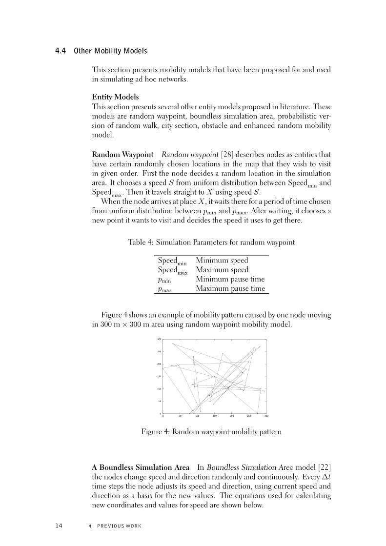
Gauss-Markov Gauss-Markov mobility model creates random movementchanges that are dependent on node’s current speed and direction. At fixedintervals the simulator generates a new speed and direction based on theircurrent values and standard deviations. In addition the model keeps nodesaway from the edges by changing their direction away from them should theyget too close.

Originally Gauss-Markov mobility model was proposed for simulating mo-bility in personal communication systems such as GSM [34]. There are manymobility models that use the same basic principle, but differ in the details.This report uses the one implemented in [6]. It uses following equations tocalculate new values for speed and direction at fixed intervals.

sn = sn−1 + α · rg · s (3)

dn = dn−1 + α · rg · α (4)

Here sn is new speed and sn−1 the current speed. dn is new direction,dn−1 the current direction, and rg a random number taken from standardGaussian distribution. s and α are the standard deviation of speed and anglefor the gaussian distribution.

The simulation parameters for Gauss-Markov mobility models are shownin Table 3

Table 3: Simulation Parameters for Gauss-Markov

Speedmax Maximum speeds Speed standard deviationα Angle standard deviationt Speed & angle update frequency

As can be seen from Figure 3, the Gauss-Markov mobility model producesmovements with smooth curves and the mobile node tends to stay away fromthe edges of the simulation area.

0

200

400

600

800

1000

0 200 400 600 800 1000 0

200

400

600

800

1000

0 200 400 600 800 1000 0

200

400

600

800

1000

0 200 400 600 800 1000

Figure 3: Gauss-Markov mobility pattern

4 PREVIOUS WORK 13

4.4 Other Mobility Models

This section presents mobility models that have been proposed for and usedin simulating ad hoc networks.

Entity ModelsThis section presents several other entity models proposed in literature. Thesemodels are random waypoint, boundless simulation area, probabilistic ver-sion of random walk, city section, obstacle and enhanced random mobilitymodel.

Random Waypoint Random waypoint [28] describes nodes as entities thathave certain randomly chosen locations in the map that they wish to visitin given order. First the node decides a random location in the simulationarea. It chooses a speed S from uniform distribution between Speedmin andSpeedmax. Then it travels straight to X using speed S.

When the node arrives at place X , it waits there for a period of time chosenfrom uniform distribution between pmin and pmax. After waiting, it chooses anew point it wants to visit and decides the speed it uses to get there.

Table 4: Simulation Parameters for random waypoint

Speedmin Minimum speedSpeedmax Maximum speedpmin Minimum pause timepmax Maximum pause time

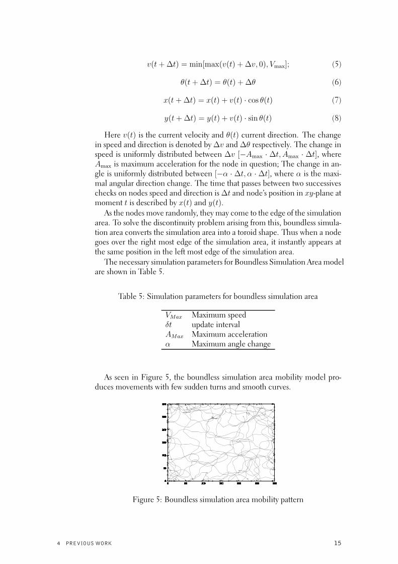
Figure 4 shows an example of mobility pattern caused by one node movingin 300 m × 300 m area using random waypoint mobility model.

0

50

100

150

200

250

300

0 50 100 150 200 250 300

Figure 4: Random waypoint mobility pattern

A Boundless Simulation Area In Boundless Simulation Area model [22]the nodes change speed and direction randomly and continuously. Every ∆ttime steps the node adjusts its speed and direction, using current speed anddirection as a basis for the new values. The equations used for calculatingnew coordinates and values for speed are shown below.

14 4 PREVIOUS WORK

v(t + ∆t) = min[max(v(t) + ∆v, 0), Vmax]; (5)

θ(t + ∆t) = θ(t) + ∆θ (6)

x(t + ∆t) = x(t) + v(t) · cos θ(t) (7)

y(t + ∆t) = y(t) + v(t) · sin θ(t) (8)

Here v(t) is the current velocity and θ(t) current direction. The changein speed and direction is denoted by ∆v and ∆θ respectively. The change inspeed is uniformly distributed between ∆v [−Amax · ∆t, Amax · ∆t], whereAmax is maximum acceleration for the node in question; The change in an-gle is uniformly distributed between [−α · ∆t, α · ∆t], where α is the maxi-mal angular direction change. The time that passes between two successiveschecks on nodes speed and direction is ∆t and node’s position in xy-plane atmoment t is described by x(t) and y(t).

As the nodes move randomly, they may come to the edge of the simulationarea. To solve the discontinuity problem arising from this, boundless simula-tion area converts the simulation area into a toroid shape. Thus when a nodegoes over the right most edge of the simulation area, it instantly appears atthe same position in the left most edge of the simulation area.

The necessary simulation parameters for Boundless Simulation Area modelare shown in Table 5.

Table 5: Simulation parameters for boundless simulation area

VMax Maximum speedδt update intervalAMax Maximum accelerationα Maximum angle change

As seen in Figure 5, the boundless simulation area mobility model pro-duces movements with few sudden turns and smooth curves.

0

50

100

150

200

250

300

0 50 100 150 200 250 300 0

50

100

150

200

250

300

0 50 100 150 200 250 300 0

50

100

150

200

250

300

0 50 100 150 200 250 300 0

50

100

150

200

250

300

0 50 100 150 200 250 300 0

50

100

150

200

250

300

0 50 100 150 200 250 300 0

50

100

150

200

250

300

0 50 100 150 200 250 300 0

50

100

150

200

250

300

0 50 100 150 200 250 300 0

50

100

150

200

250

300

0 50 100 150 200 250 300 0

50

100

150

200

250

300

0 50 100 150 200 250 300 0

50

100

150

200

250

300

0 50 100 150 200 250 300 0

50

100

150

200

250

300

0 50 100 150 200 250 300 0

50

100

150

200

250

300

0 50 100 150 200 250 300 0

50

100

150

200

250

300

0 50 100 150 200 250 300 0

50

100

150

200

250

300

0 50 100 150 200 250 300 0

50

100

150

200

250

300

0 50 100 150 200 250 300 0

50

100

150

200

250

300

0 50 100 150 200 250 300 0

50

100

150

200

250

300

0 50 100 150 200 250 300 0

50

100

150

200

250

300

0 50 100 150 200 250 300 0

50

100

150

200

250

300

0 50 100 150 200 250 300 0

50

100

150

200

250

300

0 50 100 150 200 250 300 0

50

100

150

200

250

300

0 50 100 150 200 250 300 0

50

100

150

200

250

300

0 50 100 150 200 250 300 0

50

100

150

200

250

300

0 50 100 150 200 250 300 0

50

100

150

200

250

300

0 50 100 150 200 250 300 0

50

100

150

200

250

300

0 50 100 150 200 250 300 0

50

100

150

200

250

300

0 50 100 150 200 250 300 0

50

100

150

200

250

300

0 50 100 150 200 250 300 0

50

100

150

200

250

300

0 50 100 150 200 250 300 0

50

100

150

200

250

300

0 50 100 150 200 250 300 0

50

100

150

200

250

300

0 50 100 150 200 250 300 0

50

100

150

200

250

300

0 50 100 150 200 250 300 0

50

100

150

200

250

300

0 50 100 150 200 250 300 0

50

100

150

200

250

300

0 50 100 150 200 250 300 0

50

100

150

200

250

300

0 50 100 150 200 250 300 0

50

100

150

200

250

300

0 50 100 150 200 250 300 0

50

100

150

200

250

300

0 50 100 150 200 250 300 0

50

100

150

200

250

300

0 50 100 150 200 250 300 0

50

100

150

200

250

300

0 50 100 150 200 250 300 0

50

100

150

200

250

300

0 50 100 150 200 250 300 0

50

100

150

200

250

300

0 50 100 150 200 250 300 0

50

100

150

200

250

300

0 50 100 150 200 250 300 0

50

100

150

200

250

300

0 50 100 150 200 250 300 0

50

100

150

200

250

300

0 50 100 150 200 250 300 0

50

100

150

200

250

300

0 50 100 150 200 250 300 0

50

100

150

200

250

300

0 50 100 150 200 250 300 0

50

100

150

200

250

300

0 50 100 150 200 250 300 0

50

100

150

200

250

300

0 50 100 150 200 250 300 0

50

100

150

200

250

300

0 50 100 150 200 250 300 0

50

100

150

200

250

300

0 50 100 150 200 250 300 0

50

100

150

200

250

300

0 50 100 150 200 250 300 0

50

100

150

200

250

300

0 50 100 150 200 250 300 0

50

100

150

200

250

300

0 50 100 150 200 250 300 0

50

100

150

200

250

300

0 50 100 150 200 250 300 0

50

100

150

200

250

300

0 50 100 150 200 250 300 0

50

100

150

200

250

300

0 50 100 150 200 250 300 0

50

100

150

200

250

300

0 50 100 150 200 250 300 0

50

100

150

200

250

300

0 50 100 150 200 250 300 0

50

100

150

200

250

300

0 50 100 150 200 250 300 0

50

100

150

200

250

300

0 50 100 150 200 250 300 0

50

100

150

200

250

300

0 50 100 150 200 250 300 0

50

100

150

200

250

300

0 50 100 150 200 250 300 0

50

100

150

200

250

300

0 50 100 150 200 250 300 0

50

100

150

200

250

300

0 50 100 150 200 250 300 0

50

100

150

200

250

300

0 50 100 150 200 250 300 0

50

100

150

200

250

300

0 50 100 150 200 250 300 0

50

100

150

200

250

300

0 50 100 150 200 250 300 0

50

100

150

200

250

300

0 50 100 150 200 250 300 0

50

100

150

200

250

300

0 50 100 150 200 250 300 0

50

100

150

200

250

300

0 50 100 150 200 250 300 0

50

100

150

200

250

300

0 50 100 150 200 250 300 0

50

100

150

200

250

300

0 50 100 150 200 250 300 0

50

100

150

200

250

300

0 50 100 150 200 250 300 0

50

100

150

200

250

300

0 50 100 150 200 250 300 0

50

100

150

200

250

300

0 50 100 150 200 250 300 0

50

100

150

200

250

300

0 50 100 150 200 250 300 0

50

100

150

200

250

300

0 50 100 150 200 250 300 0

50

100

150

200

250

300

0 50 100 150 200 250 300 0

50

100

150

200

250

300

0 50 100 150 200 250 300 0

50

100

150

200

250

300

0 50 100 150 200 250 300 0

50

100

150

200

250

300

0 50 100 150 200 250 300 0

50

100

150

200

250

300

0 50 100 150 200 250 300 0

50

100

150

200

250

300

0 50 100 150 200 250 300 0

50

100

150

200

250

300

0 50 100 150 200 250 300 0

50

100

150

200

250

300

0 50 100 150 200 250 300 0

50

100

150

200

250

300

0 50 100 150 200 250 300 0

50

100

150

200

250

300

0 50 100 150 200 250 300 0

50

100

150

200

250

300

0 50 100 150 200 250 300 0

50

100

150

200

250

300

0 50 100 150 200 250 300 0

50

100

150

200

250

300

0 50 100 150 200 250 300 0

50

100

150

200

250

300

0 50 100 150 200 250 300 0

50

100

150

200

250

300

0 50 100 150 200 250 300 0

50

100

150

200

250

300

0 50 100 150 200 250 300 0

50

100

150

200

250

300

0 50 100 150 200 250 300 0

50

100

150

200

250

300

0 50 100 150 200 250 300 0

50

100

150

200

250

300

0 50 100 150 200 250 300 0

50

100

150

200

250

300

0 50 100 150 200 250 300 0

50

100

150

200

250

300

0 50 100 150 200 250 300 0

50

100

150

200

250

300

0 50 100 150 200 250 300 0

50

100

150

200

250

300

0 50 100 150 200 250 300 0

50

100

150

200

250

300

0 50 100 150 200 250 300 0

50

100

150

200

250

300

0 50 100 150 200 250 300 0

50

100

150

200

250

300

0 50 100 150 200 250 300 0

50

100

150

200

250

300

0 50 100 150 200 250 300 0

50

100

150

200

250

300

0 50 100 150 200 250 300 0

50

100

150

200

250

300

0 50 100 150 200 250 300 0

50

100

150

200

250

300

0 50 100 150 200 250 300 0

50

100

150

200

250

300

0 50 100 150 200 250 300 0

50

100

150

200

250

300

0 50 100 150 200 250 300 0

50

100

150

200

250

300

0 50 100 150 200 250 300 0

50

100

150

200

250

300

0 50 100 150 200 250 300 0

50

100

150

200

250

300

0 50 100 150 200 250 300 0

50

100

150

200

250

300

0 50 100 150 200 250 300 0

50

100

150

200

250

300

0 50 100 150 200 250 300 0

50

100

150

200

250

300

0 50 100 150 200 250 300 0

50

100

150

200

250

300

0 50 100 150 200 250 300 0

50

100

150

200

250

300

0 50 100 150 200 250 300 0

50

100

150

200

250

300

0 50 100 150 200 250 300 0

50

100

150

200

250

300

0 50 100 150 200 250 300 0

50

100

150

200

250

300

0 50 100 150 200 250 300 0

50

100

150

200

250

300

0 50 100 150 200 250 300 0

50

100

150

200

250

300

0 50 100 150 200 250 300 0

50

100

150

200

250

300

0 50 100 150 200 250 300 0

50

100

150

200

250

300

0 50 100 150 200 250 300 0

50

100

150

200

250

300

0 50 100 150 200 250 300 0

50

100

150

200

250

300

0 50 100 150 200 250 300 0

50

100

150

200

250

300

0 50 100 150 200 250 300 0

50

100

150

200

250

300

0 50 100 150 200 250 300 0

50

100

150

200

250

300

0 50 100 150 200 250 300 0

50

100

150

200

250

300

0 50 100 150 200 250 300 0

50

100

150

200

250

300

0 50 100 150 200 250 300 0

50

100

150

200

250

300

0 50 100 150 200 250 300 0

50

100

150

200

250

300

0 50 100 150 200 250 300 0

50

100

150

200

250

300

0 50 100 150 200 250 300 0

50

100

150

200

250

300

0 50 100 150 200 250 300 0

50

100

150

200

250

300

0 50 100 150 200 250 300 0

50

100

150

200

250

300

0 50 100 150 200 250 300 0

50

100

150

200

250

300

0 50 100 150 200 250 300 0

50

100

150

200

250

300

0 50 100 150 200 250 300 0

50

100

150

200

250

300

0 50 100 150 200 250 300 0

50

100

150

200

250

300

0 50 100 150 200 250 300 0

50

100

150

200

250

300

0 50 100 150 200 250 300 0

50

100

150

200

250

300

0 50 100 150 200 250 300 0

50

100

150

200

250

300

0 50 100 150 200 250 300 0

50

100

150

200

250

300

0 50 100 150 200 250 300 0

50

100

150

200

250

300

0 50 100 150 200 250 300 0

50

100

150

200

250

300

0 50 100 150 200 250 300 0

50

100

150

200

250

300

0 50 100 150 200 250 300 0

50

100

150

200

250

300

0 50 100 150 200 250 300 0

50

100

150

200

250

300

0 50 100 150 200 250 300 0

50

100

150

200

250

300

0 50 100 150 200 250 300 0

50

100

150

200

250

300

0 50 100 150 200 250 300 0

50

100

150

200

250

300

0 50 100 150 200 250 300 0

50

100

150

200

250

300

0 50 100 150 200 250 300 0

50

100

150

200

250

300

0 50 100 150 200 250 300 0

50

100

150

200

250

300

0 50 100 150 200 250 300 0

50

100

150

200

250

300

0 50 100 150 200 250 300 0

50

100

150

200

250

300

0 50 100 150 200 250 300 0

50

100

150

200

250

300

0 50 100 150 200 250 300 0

50

100

150

200

250

300

0 50 100 150 200 250 300 0

50

100

150

200

250

300

0 50 100 150 200 250 300 0

50

100

150

200

250

300

0 50 100 150 200 250 300 0

50

100

150

200

250

300

0 50 100 150 200 250 300 0

50

100

150

200

250

300

0 50 100 150 200 250 300 0

50

100

150

200

250

300

0 50 100 150 200 250 300 0

50

100

150

200

250

300

0 50 100 150 200 250 300 0

50

100

150

200

250

300

0 50 100 150 200 250 300 0

50

100

150

200

250

300

0 50 100 150 200 250 300 0

50

100

150

200

250

300

0 50 100 150 200 250 300 0

50

100

150

200

250

300

0 50 100 150 200 250 300 0

50

100

150

200

250

300

0 50 100 150 200 250 300 0

50

100

150

200

250

300

0 50 100 150 200 250 300 0

50

100

150

200

250

300

0 50 100 150 200 250 300 0

50

100

150

200

250

300

0 50 100 150 200 250 300 0

50

100

150

200

250

300

0 50 100 150 200 250 300 0

50

100

150

200

250

300

0 50 100 150 200 250 300 0

50

100

150

200

250

300

0 50 100 150 200 250 300 0

50

100

150

200

250

300

0 50 100 150 200 250 300 0

50

100

150

200

250

300

0 50 100 150 200 250 300 0

50

100

150

200

250

300

0 50 100 150 200 250 300 0

50

100

150

200

250

300

0 50 100 150 200 250 300 0

50

100

150

200

250

300

0 50 100 150 200 250 300 0

50

100

150

200

250

300

0 50 100 150 200 250 300 0

50

100

150

200

250

300

0 50 100 150 200 250 300 0

50

100

150

200

250

300

0 50 100 150 200 250 300 0

50

100

150

200

250

300

0 50 100 150 200 250 300 0

50

100

150

200

250

300

0 50 100 150 200 250 300 0

50

100

150

200

250

300

0 50 100 150 200 250 300 0

50

100

150

200

250

300

0 50 100 150 200 250 300 0

50

100

150

200

250

300

0 50 100 150 200 250 300 0

50

100

150

200

250

300

0 50 100 150 200 250 300 0

50

100

150

200

250

300

0 50 100 150 200 250 300 0

50

100

150

200

250

300

0 50 100 150 200 250 300 0

50

100

150

200

250

300

0 50 100 150 200 250 300 0

50

100

150

200

250

300

0 50 100 150 200 250 300 0

50

100

150

200

250

300

0 50 100 150 200 250 300 0

50

100

150

200

250

300

0 50 100 150 200 250 300 0

50

100

150

200

250

300

0 50 100 150 200 250 300 0

50

100

150

200

250

300

0 50 100 150 200 250 300 0

50

100

150

200

250

300

0 50 100 150 200 250 300 0

50

100

150

200

250

300

0 50 100 150 200 250 300 0

50

100

150

200

250

300

0 50 100 150 200 250 300 0

50

100

150

200

250

300

0 50 100 150 200 250 300 0

50

100

150

200

250

300

0 50 100 150 200 250 300 0

50

100

150

200

250

300

0 50 100 150 200 250 300 0

50

100

150

200

250

300

0 50 100 150 200 250 300 0

50

100

150

200

250

300

0 50 100 150 200 250 300 0

50

100

150

200

250

300

0 50 100 150 200 250 300 0

50

100

150

200

250

300

0 50 100 150 200 250 300 0

50

100

150

200

250

300

0 50 100 150 200 250 300 0

50

100

150

200

250

300

0 50 100 150 200 250 300 0

50

100

150

200

250

300

0 50 100 150 200 250 300 0

50

100

150

200

250

300

0 50 100 150 200 250 300 0

50

100

150

200

250

300

0 50 100 150 200 250 300 0

50

100

150

200

250

300

0 50 100 150 200 250 300 0

50

100

150

200

250

300

0 50 100 150 200 250 300 0

50

100

150

200

250

300

0 50 100 150 200 250 300 0

50

100

150

200

250

300

0 50 100 150 200 250 300 0

50

100

150

200

250

300

0 50 100 150 200 250 300 0

50

100

150

200

250

300

0 50 100 150 200 250 300 0

50

100

150

200

250

300

0 50 100 150 200 250 300 0

50

100

150

200

250

300

0 50 100 150 200 250 300 0

50

100

150

200

250

300

0 50 100 150 200 250 300 0

50

100

150

200

250

300

0 50 100 150 200 250 300 0

50

100

150

200

250

300

0 50 100 150 200 250 300 0

50

100

150

200

250

300

0 50 100 150 200 250 300 0

50

100

150

200

250

300

0 50 100 150 200 250 300 0

50

100

150

200

250

300

0 50 100 150 200 250 300 0

50

100

150

200

250

300

0 50 100 150 200 250 300 0

50

100

150

200

250

300

0 50 100 150 200 250 300 0

50

100

150

200

250

300

0 50 100 150 200 250 300 0

50

100

150

200

250

300

0 50 100 150 200 250 300 0

50

100

150

200

250

300

0 50 100 150 200 250 300 0

50

100

150

200

250

300

0 50 100 150 200 250 300 0

50

100

150

200

250

300

0 50 100 150 200 250 300

Figure 5: Boundless simulation area mobility pattern

4 PREVIOUS WORK 15

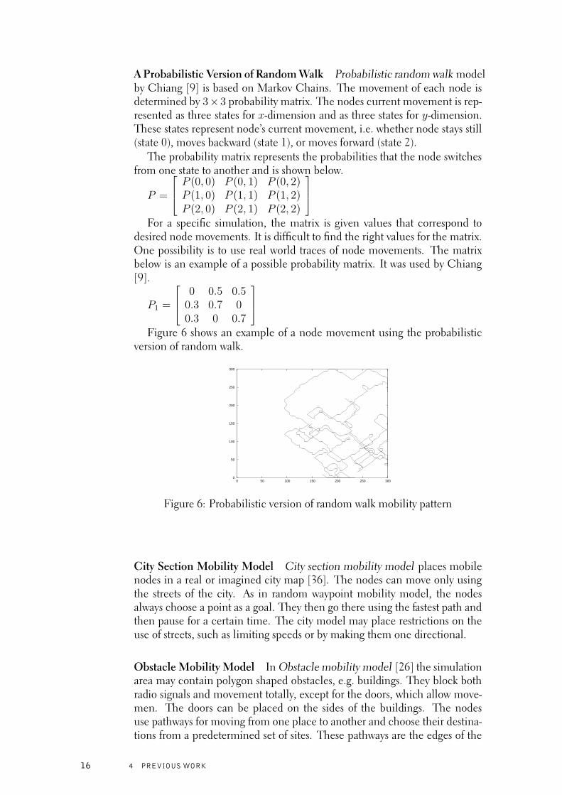
A Probabilistic Version of Random Walk Probabilistic random walk modelby Chiang [9] is based on Markov Chains. The movement of each node isdetermined by 3× 3 probability matrix. The nodes current movement is rep-resented as three states for x-dimension and as three states for y-dimension.These states represent node’s current movement, i.e. whether node stays still(state 0), moves backward (state 1), or moves forward (state 2).

The probability matrix represents the probabilities that the node switchesfrom one state to another and is shown below.

P =

P (0, 0) P (0, 1) P (0, 2)P (1, 0) P (1, 1) P (1, 2)P (2, 0) P (2, 1) P (2, 2)

For a specific simulation, the matrix is given values that correspond todesired node movements. It is difficult to find the right values for the matrix.One possibility is to use real world traces of node movements. The matrixbelow is an example of a possible probability matrix. It was used by Chiang[9].

P1 =

0 0.5 0.50.3 0.7 00.3 0 0.7

Figure 6 shows an example of a node movement using the probabilisticversion of random walk.

0

50

100

150

200

250

300

0 50 100 150 200 250 300

Figure 6: Probabilistic version of random walk mobility pattern

City Section Mobility Model City section mobility model places mobilenodes in a real or imagined city map [36]. The nodes can move only usingthe streets of the city. As in random waypoint mobility model, the nodesalways choose a point as a goal. They then go there using the fastest path andthen pause for a certain time. The city model may place restrictions on theuse of streets, such as limiting speeds or by making them one directional.

Obstacle Mobility Model In Obstacle mobility model [26] the simulationarea may contain polygon shaped obstacles, e.g. buildings. They block bothradio signals and movement totally, except for the doors, which allow move-men. The doors can be placed on the sides of the buildings. The nodesuse pathways for moving from one place to another and choose their destina-tions from a predetermined set of sites. These pathways are the edges of the

16 4 PREVIOUS WORK

Voronoi-diagram [14] over the simulation area using the corners of obstaclesas dividing points.

Voronoi-diagram partitions a plane into cells using a set of dividing pointson the plane. The partition is such that each cell contains exactly one of thesedividing points. In addition at each point on the plane, the closest dividingpoint is in the same cell as the point itself. In other words, the edges betweencells consist of those points in which the distance to the closest location pointsis the same.

When a node chooses a destination, it first travels directly to an edge onthe Voronoid graph, and then uses the shortest proute to the destination suchthat it stays on the edges of the graph.

Table 6 shows the simulation parameters for the obstacle mobility model.

Table 6: Simulation parameters for obstacle model

V Speed distributiondi The destination sitesp Pause time distribution

Smooth Mobility Model In smooth mobility model [5] a node choosesa direction and then starts accelerating to change its velocity to the chosendirection. The node also chooses a certain amount of time that it will travelto that direction before it chooses a new direction. Both of these decisionsare controlled by stochastic processes.

This creates movements that is smooth and more realistic, because reallife acceleration capabilities are taken into account.

Group Mobility Models

This section presents group models proposed in literature. These models arepursue, nomadic community, column and reference point group mobilitymodel (RPGM).

Pursue Mobility Model Pursue mobility model [48] describes a group ofnodes that are trying to catch a runaway node. Each node tries to move asclose to the runaway nodes current position as possible. The position updatesare done using the following equation, where P (x, y, t) describes the nodesposition at time t. R is a random vector, which controls how well the nodesare capable of following their prey and D is a vector toward the runaway node.The vector D is between Dmin and Dmax specified as simulation parametersand such that without the random vector, the node would end up as close tothe runaway nodes location as possible.

P (x, y, t + ∆t) = P (x, y, t) + D + R

Nomadic Community Mobility Model Nomadic community model [48]represents a group of people moving from one location to another. This is

4 PREVIOUS WORK 17

simulated so that each group has a reference point that moves toward thegroup destination. Each member of the group roams around the group ref-erence point using an entity mobility model (e.g. random walk). When thereference point is updated, all nodes start travel to the area defined by thenew reference point and then start wandering again.

Column Mobility Model In column mobility model [48], each node hasa certain place in a column just as one might have in a search/rescue oper-ation. The column moves forward at a constant speed. The new referencepoint for a node can be calculated using newReferencePoint = oldReferencePoint+advanceVector equation. Each node is allowed to move randomly around itsreference point. This node movement is accomplished using some entitymobility model, such as random walk.

Reference Point Group Mobility Model Reference point group mobilitymodel (RPGM) [24] separates the motion of the group and the motion ofeach node in the group. Each group has a motion vector Vgi

. Each nodeis assigned a reference point with relation to the group reference point. Amovement of a node is done so that first the reference point of the node istransferred using the group motion vector and then the node’s position israndomly varied around the reference point. The random vector that is usedfor varying the position is uniformly distributed between 0 and 360 degreeand between 0 and certain predefined length.

Individually Simulated Mobility Model

The individually simulated mobility model cannot be categorized as entitymobility model, nor as group mobility model.

In individually simulated mobility model [49] each node has a decisionsystem that makes decisions about movements. This system consists of threecomponents: the perception component, the behavioral component andthe movement component. The perception component provides informa-tion about the immediate surroundings of the node. The behavioral modelchooses what actions the node should make based on the perception infor-mation and the movement component executes these actions.

The behavioral model is built with four rules: Group centering, collisionavoidance, velocity matching and inertia. Each of these rules takes its priority(between 0 and 1) as simulation parameter. Group centering means thatnodes want to be at the center of the group that they can percept; collisionavoidance means that nodes want to avoid getting too close to other nodes;velocity matching means that nodes wish to match their velocity with thosein their immediate surroundings and inertia tells how fast they can changetheir velocity vector.

These potentially conflicting desires are combined by using a weightedsum over acceleration requests provided by each rule.

4.5 Simulators

Network Simulator 2 (NS2) [38] is a discrete event simulator targeted at net-working research. It includes support for both wireless networking and wired

18 4 PREVIOUS WORK

networking. It is implemented combining C++ and TCL, so that scriptingdifferent networking scenarios with TCL is easy while adding new protocolsand features to the underlying simulator is efficient using compiled C++code. In addition to this, NS2 is widely used in ad hoc networks research.Thus using NS2 makes the results more comparable to other work done inthe field. These factors made NS2 an ideal choice for this work.

The code providing Random Walk and Random Direction mobility wasprovided by Camp et al [8]. The code providing Gauss-Markov mobility wasprovided by BonnMotion group [6].

There are other network simulators that support ad hoc networking tosome degree, e.g. PARSEC [1] and Glomosim [19].

4 PREVIOUS WORK 19

5 MEASURING MOBILITY

Routing in ad hoc networks is harder than in traditional networks. This ismainly due to the fact that in traditional networks links between nodes donot change, or change very slowly in time. Thus key difference betweenthese types of networks is the dynamicity of links and the lack of specificinfrastructure designed to handle network control.

Route life time distribution is an important metric for understanding theeffects of mobility on reactive ad hoc routing [47, 50]. This Chapter proposesan experimental method for measuring the route lifetime distribution.

5.1 Dynamic Networks

A dynamic network can be considered as a set of graphs that is ordered bytime. This discussion considers a discrete time in which ∆t is the smallesttime step. From here on, the this set of graphs is referred just as a graph. Ifthere is a possibility of a confusion between this and ordinary graphs, theywill be referred as a dynamic and an ordinary graphs.

A graph can be expressed as

G[t] = (V, E[t])

Let (A, B)[t] = 1 denote that a link between A and B exists in G[t], i.e. alink exists at time t. Similarly let (A, B)[t] = 0 denote that no link between Aand B exists in G[t]. If ∀t, t0 ≤ t ≤ t1 (A, B)[t] = 1 and (A, B)[t1+∆t] = 0,then the remaining life link time (llt) of the link between A and B at time t0is llt = t1 − t0.

llt is thus the time that link is continuously up from a given moment to itsdestruction. This concept is used, because when ad hoc routes are formed,the links that are used for it are those that are available at the particular timeof forming the link.

5.2 Distance Distribution

The distance distribution for an ordinary graph describes the discrete prob-ability distribution for the distance of randomly chosen pair of nodes. Thedistance of a pair of nodes is defined in Section 4.1.

The distance distribution can be calculated by calculating the number ofnode pairs N(i) within distance i, i = 1, 2, 3, . . .. The probability distribution

P (i) is then P (i) = N(i)n·(n−1)

2

, where n is the number of nodes. The distance

distribution of a set of k graphs is the average of their respective distancedistributions.

The distance distribution of an ad hoc network for a given mobility modelwith certain parameters can be measured with simulation. The formula isfollowing:

Run n simulations with given mobility model and parameters.Choose a moment between (t, tmax) and measure the distance distribu-

tion at that point. The initial spatial distribution of nodes does not necessar-ily resemble the distribution that the mobility model produces. Because of

20 5 MEASURING MOBILITY

this t � 0 is required in order to let the spatial distribution resemble thatproduced by the model rather than the initial distribution.

Calculate the distribution using these samples and scale it to have theprobabilities sum to 1.

5.3 Measuring Remaining Link Life Time Distribution

The llt distribution describes the probability distribution of the remaininglife time of a randomly chosen link at given time t.

To find the llt probability distribution, n simulations are run. A certainmoment is chosen from uniform distribution between (t1, t2), where t1 � 0and t2 � tmax. The former is a requirement, because the initial spatialdistribution may not resemble one created by the mobility model and thelatter, because the chosen time should be such that no link lasts until theend of the simulation. If some links last from the chosen time point till theend of the simulation, then the estimate of llt will be too small.llt will then be calculated for each link that exists.

The distribution that we get is the distribution of remaining link lifetimesfor those links that exist at certain moment. It is not the life time distributionfor randomly chosen link at the time of its birth. This is chosen, because alllinks in a route are chosen at a particular moment.

5.4 Route Life Time Distribution (rlt)

This report proposes that the life time distribution of the shortest route (routelife time distribution rlt) between two random nodes is a good metrics forthe impact of mobility for ad hoc routing. The model assumes that the lltdistributions of links in this route are independent of each other and thatthe distribution is the same as the llt distribution produced by the mobilitymodel. This assumption is not valid, since the two links that a node partic-ipates in within a route are dependent on each other. Still, it should be agood enough approximation.

The life time distribution of a route between two random nodes can becalculated, if the distance distribution of nodes and life time distribution oflinks is known. These can be measured from simulation samples. The routelife time distribution is calculated as follows.

Measure the distance distribution and link life time distribution from thesamples.

1. Let P (p1, . . . , pn) be a discrete distance distribution, where pi denotesthe probability that the distance between two random nodes in a graphis i. This can be measured from simulation samples.

2. Let f be a continuous density such that∫ ba f = P (a ≤ X ≤ b) denotes

the probability that the remaining link life time is between a and b.Then F (t) =

∫

t −∞tf is the cumulative link life time distribution.

3. The remaining life time distribution of a given route can be calculatedin following manner. It is assumed that the lifetime of each link in aroute is randomly selected from the given density function.

5 MEASURING MOBILITY 21

4. Let

G(t) = 1 − F (t) (9)

be the probability that at time t the link has not yet broken. Then theprobability that none of i random links has yet broken is G(t)i.

Thus the cumulative random distribution that the route is still valid t sec-onds after creation is thus

F(t) = Σni=1PiG(t)i (10)

The rlt distribution F describes how long communications between twonodes will continue before the route has to be renewed.

Eventually we will want to compare rlt distributions from different mobil-ity models and judge their relative difficulty for reactive ad hoc routing foreach other.

The ranking system has to meet the following criterion:If ∀t FA(t) ≤ FBt then A must be ranked more difficult mobility than B.

There are three obvious ways of ranking the distributions and each has itsproblems. These are average route life time; median, or any given percentileof route life time; and measuring what percentage of routes are still valid aftert seconds.

Average Route Life Time

Under ordinary circumstances average route life time measurement gives agood understanding of how long on average a route will last. However, if themobility model produces some links that live forever, as some group mobilitymodels do, then the rlt distribution will contain a non-zero portion of routeswith infinite lifetime.

Non-zero portion of routes with infinite lifetime automatically raise the ex-pected route life time to infinity. Thus average route life time measurementfails to convey important information about relative hardness of different rltdistributions.

Percentile of Route Life Time

Choosing a certain percentile to represent the difficulties posed by the mo-bility is another possibility. The question is, which percentile would be rep-resentative for ranking different rlt distributions.

The problem of using any pre-determined percentile is that it lumps to-gether many different scenarios in which rlt of the given percentile is zero.This is possible, because the rlt distribution includes in itself those communi-cation attempts that happen between nodes that are disconnected from eachother.

Percentage of Routes Valid After t Seconds

Another possibility is to measure what portion of routes is still valid after a pre-determined time. This means that meaningful comparisons cannot be madebased on this criteria, if a very small, or big portion of the routes survive tothe given time limit.

22 5 MEASURING MOBILITY

Proposed VariantI propose that median of rlt should be used, when that median is greater thanzero. If the median is zero, then the percentage of routes with a lifetime atleast one seconds should be used.

This approach has the good qualities of median of rlt and still gives ameaningful basis for comparison on those cases, where more than 50% ofroutes last less than 1 second.

5 MEASURING MOBILITY 23

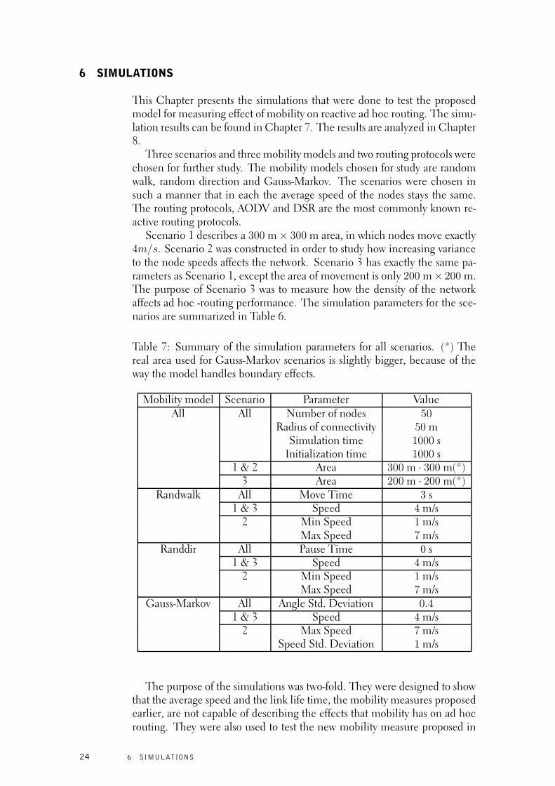
6 SIMULATIONS

This Chapter presents the simulations that were done to test the proposedmodel for measuring effect of mobility on reactive ad hoc routing. The simu-lation results can be found in Chapter 7. The results are analyzed in Chapter8.

Three scenarios and three mobility models and two routing protocols werechosen for further study. The mobility models chosen for study are randomwalk, random direction and Gauss-Markov. The scenarios were chosen insuch a manner that in each the average speed of the nodes stays the same.The routing protocols, AODV and DSR are the most commonly known re-active routing protocols.

Scenario 1 describes a 300 m × 300 m area, in which nodes move exactly4m/s. Scenario 2 was constructed in order to study how increasing varianceto the node speeds affects the network. Scenario 3 has exactly the same pa-rameters as Scenario 1, except the area of movement is only 200 m× 200 m.The purpose of Scenario 3 was to measure how the density of the networkaffects ad hoc -routing performance. The simulation parameters for the sce-narios are summarized in Table 6.

Table 7: Summary of the simulation parameters for all scenarios. (*) Thereal area used for Gauss-Markov scenarios is slightly bigger, because of theway the model handles boundary effects.

Mobility model Scenario Parameter ValueAll All Number of nodes 50

Radius of connectivity 50 mSimulation time 1000 s

Initialization time 1000 s1 & 2 Area 300 m · 300 m(*)

3 Area 200 m · 200 m(*)Randwalk All Move Time 3 s

1 & 3 Speed 4 m/s2 Min Speed 1 m/s

Max Speed 7 m/sRanddir All Pause Time 0 s

1 & 3 Speed 4 m/s2 Min Speed 1 m/s

Max Speed 7 m/sGauss-Markov All Angle Std. Deviation 0.4

1 & 3 Speed 4 m/s2 Max Speed 7 m/s

Speed Std. Deviation 1 m/s

The purpose of the simulations was two-fold. They were designed to showthat the average speed and the link life time, the mobility measures proposedearlier, are not capable of describing the effects that mobility has on ad hocrouting. They were also used to test the new mobility measure proposed in

24 6 SIMULATIONS

this report.The simulations were done in two phases.The first part of the simulations measured the route life time (rlt) for each

mobility model for each scenario. Using these measurements these 9 differ-ent scenarios will be ranked by the relative difficulty they pose for reactive adhoc routing.

The second part of the simulations used the same scenarios and same mo-bility models. The purpose of these simulations was to measure the perfor-mance of two routing protocols, AODV and DSR. The basis of performancemeasurements is from Broch et al. [7] and Johansson et al. [27]. If the modelproposed in this report is correct, then the performance results should reflectthe ranking from the first set of simulations.

6.1 Finding Route Life Time Distribution

Three mobility models, random walk, random direction and Gauss-Markov,were sampled to find their route life time (rlt) distribution for different pa-rameter values. Each model was simulated 1000 times for each scenario.The rlt distribution is used to predict the difficulty each scenario presents toad hoc routing. The method for estimating rlt is described in Chapter 5.

Table 9 shows the distance distribution created by Random Walk in Sce-narios 1 and 2 and 3. The results are organized such that each column showsthe whole distance distribution for one scenario and each row shows the prob-ability that two nodes are at a certain distance. For example value 1.1% inrow 10 and column 2 indicates the probability that the distance between twonodes is 10 in Scenario 2.

Similarly, tables 10 and 11 show the distance distribution results for Sce-narios 1 and 2 and 3 with Random Direction and Gauss-Markov.

The llt distributions were measured as defined in Section 5.3. Figure 7shows the llt distribution for random walk in Scenarios 1, 2 and 3. A point(t, p) in the graph expresses the probability that a randomly selected linksurvives at least t seconds from the moment the observation is started.Similarly 8 and 9 show the llt distribution for random direction and Gauss-Markov mobility models for each scenario.

The rlt distributions were calculated from these measurements. Figure10 shows the rlt results for random walk in Scenarios 1, 2 and 3. The distri-bution shown is the F distribution defined in Equation 10. A point (t, p) inthe graph expresses the probability that the shortest path between randomlyselected pair of nodes survives at least t seconds from the moment the obser-vation is started.

Similarly 11 and 12 show the rlt distribution for random direction andGauss-Markov mobility models for each scenario.

6.2 Simulation Results for Testing Hypothesis

This section provides the description and results of the simulations for testingthe hypothesis. The hypothesis is that those mobility models with certainparameters that were rated more difficult in previous chapter will produce

6 SIMULATIONS 25

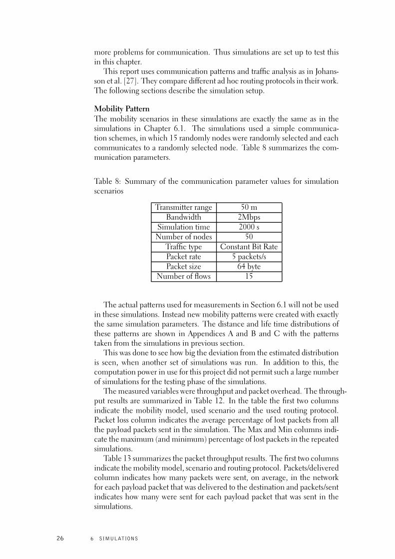
more problems for communication. Thus simulations are set up to test thisin this chapter.

This report uses communication patterns and traffic analysis as in Johans-son et al. [27]. They compare different ad hoc routing protocols in their work.The following sections describe the simulation setup.

Mobility PatternThe mobility scenarios in these simulations are exactly the same as in thesimulations in Chapter 6.1. The simulations used a simple communica-tion schemes, in which 15 randomly nodes were randomly selected and eachcommunicates to a randomly selected node. Table 8 summarizes the com-munication parameters.

Table 8: Summary of the communication parameter values for simulationscenarios

Transmitter range 50 mBandwidth 2Mbps

Simulation time 2000 sNumber of nodes 50

Traffic type Constant Bit RatePacket rate 5 packets/sPacket size 64 byte

Number of flows 15

The actual patterns used for measurements in Section 6.1 will not be usedin these simulations. Instead new mobility patterns were created with exactlythe same simulation parameters. The distance and life time distributions ofthese patterns are shown in Appendices A and B and C with the patternstaken from the simulations in previous section.

This was done to see how big the deviation from the estimated distributionis seen, when another set of simulations was run. In addition to this, thecomputation power in use for this project did not permit such a large numberof simulations for the testing phase of the simulations.

The measured variables were throughput and packet overhead. The through-put results are summarized in Table 12. In the table the first two columnsindicate the mobility model, used scenario and the used routing protocol.Packet loss column indicates the average percentage of lost packets from allthe payload packets sent in the simulation. The Max and Min columns indi-cate the maximum (and minimum) percentage of lost packets in the repeatedsimulations.

Table 13 summarizes the packet throughput results. The first two columnsindicate the mobility model, scenario and routing protocol. Packets/deliveredcolumn indicates how many packets were sent, on average, in the networkfor each payload packet that was delivered to the destination and packets/sentindicates how many were sent for each payload packet that was sent in thesimulations.

26 6 SIMULATIONS

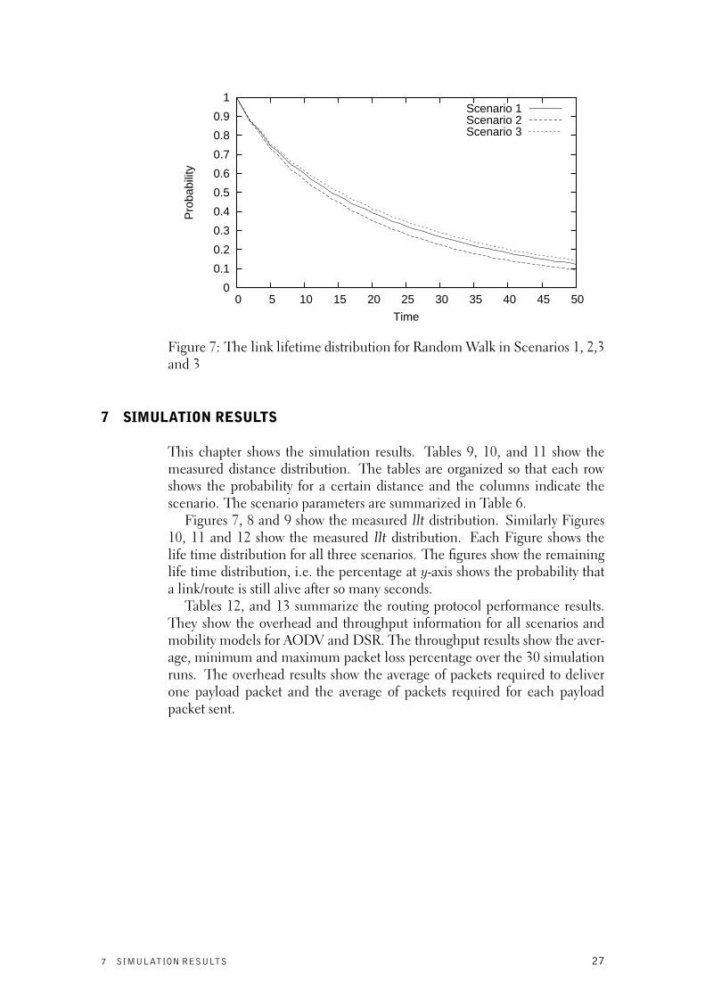
0

0.1

0.2

0.3

0.4

0.5

0.6

0.7

0.8

0.9

1

0 5 10 15 20 25 30 35 40 45 50

Pro

babi

lity

Time

Scenario 1Scenario 2Scenario 3

Figure 7: The link lifetime distribution for Random Walk in Scenarios 1, 2,3and 3

7 SIMULATION RESULTS

This chapter shows the simulation results. Tables 9, 10, and 11 show themeasured distance distribution. The tables are organized so that each rowshows the probability for a certain distance and the columns indicate thescenario. The scenario parameters are summarized in Table 6.

Figures 7, 8 and 9 show the measured llt distribution. Similarly Figures10, 11 and 12 show the measured llt distribution. Each Figure shows thelife time distribution for all three scenarios. The figures show the remaininglife time distribution, i.e. the percentage at y-axis shows the probability thata link/route is still alive after so many seconds.

Tables 12, and 13 summarize the routing protocol performance results.They show the overhead and throughput information for all scenarios andmobility models for AODV and DSR. The throughput results show the aver-age, minimum and maximum packet loss percentage over the 30 simulationruns. The overhead results show the average of packets required to deliverone payload packet and the average of packets required for each payloadpacket sent.

7 SIMULATION RESULTS 27

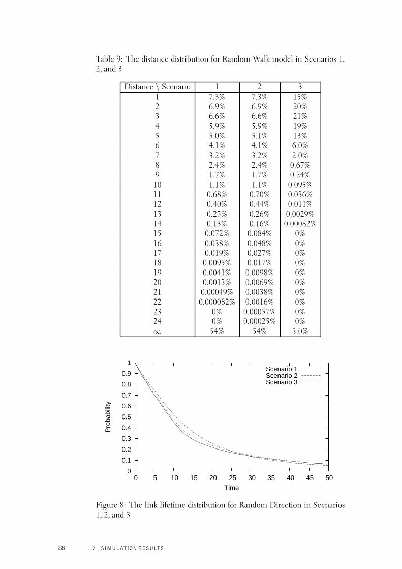
Table 9: The distance distribution for Random Walk model in Scenarios 1,2, and 3

Distance \ Scenario 1 2 31 7.3% 7.3% 15%2 6.9% 6.9% 20%3 6.6% 6.6% 21%4 5.9% 5.9% 19%5 5.0% 5.1% 13%6 4.1% 4.1% 6.0%7 3.2% 3.2% 2.0%8 2.4% 2.4% 0.67%9 1.7% 1.7% 0.24%

10 1.1% 1.1% 0.095%11 0.68% 0.70% 0.036%12 0.40% 0.44% 0.011%13 0.23% 0.26% 0.0029%14 0.13% 0.16% 0.00082%15 0.072% 0.084% 0%16 0.038% 0.048% 0%17 0.019% 0.027% 0%18 0.0095% 0.017% 0%19 0.0041% 0.0098% 0%20 0.0013% 0.0069% 0%21 0.00049% 0.0038% 0%22 0.000082% 0.0016% 0%23 0% 0.00057% 0%24 0% 0.00025% 0%∞ 54% 54% 3.0%

0

0.1

0.2

0.3

0.4

0.5

0.6

0.7

0.8

0.9

1

0 5 10 15 20 25 30 35 40 45 50

Pro

babi

lity

Time


Figure 8: The link lifetime distribution for Random Direction in Scenarios1, 2, and 3

28 7 SIMULATION RESULTS

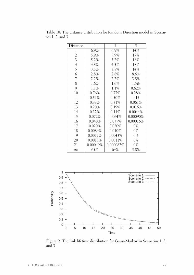
Table 10: The distance distribution for Random Direction model in Scenar-ios 1, 2, and 3

Distance 1 2 31 6.9% 6.9% 14%2 5.9% 5.9% 17%3 5.2% 5.2% 18%4 4.3% 4.3% 18%5 3.5% 3.5% 14%6 2.8% 2.8% 8.6%7 2.2% 2.2% 3.8%8 1.6% 1.6% 1.5&9 1.1% 1.1% 0.62%

10 0.76% 0.77% 0.28%11 0.51% 0.50% 0.1312 0.33% 0.31% 0.061%13 0.20% 0.19% 0.016%14 0.12% 0.11% 0.0044%15 0.072% 0.064% 0.00090%16 0.040% 0.037% 0.00016%17 0.020% 0.020% 0%18 0.0084% 0.010% 0%19 0.0055% 0.0043% 0%20 0.0015% 0.0011% 0%21 0.00049% 0.000082% 0%∞ 65% 64% 3.8%

0

0.1

0.2

0.3

0.4

0.5

0.6

0.7

0.8

0.9

1

0 5 10 15 20 25 30 35 40 45 50

Pro

babi

lity

Time


Figure 9: The link lifetime distribution for Gauss-Markov in Scenarios 1, 2,and 3


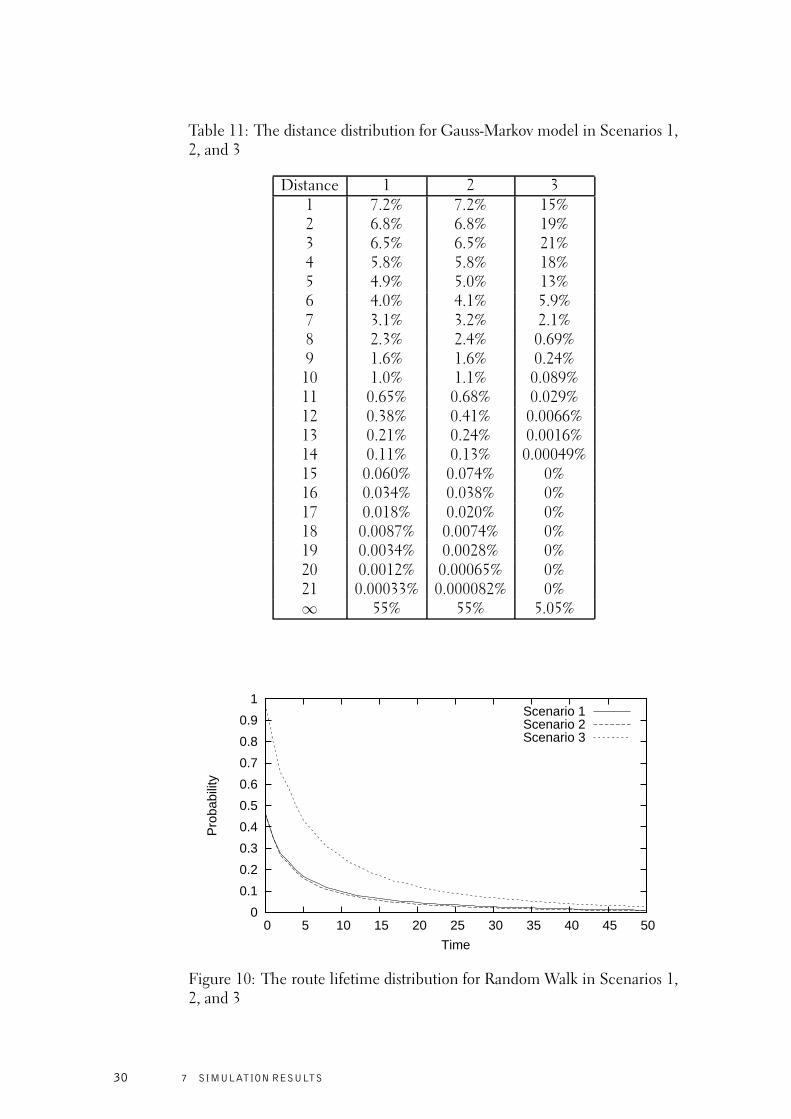
Table 11: The distance distribution for Gauss-Markov model in Scenarios 1,2, and 3

Distance 1 2 31 7.2% 7.2% 15%2 6.8% 6.8% 19%3 6.5% 6.5% 21%4 5.8% 5.8% 18%5 4.9% 5.0% 13%6 4.0% 4.1% 5.9%7 3.1% 3.2% 2.1%8 2.3% 2.4% 0.69%9 1.6% 1.6% 0.24%

10 1.0% 1.1% 0.089%11 0.65% 0.68% 0.029%12 0.38% 0.41% 0.0066%13 0.21% 0.24% 0.0016%14 0.11% 0.13% 0.00049%15 0.060% 0.074% 0%16 0.034% 0.038% 0%17 0.018% 0.020% 0%18 0.0087% 0.0074% 0%19 0.0034% 0.0028% 0%20 0.0012% 0.00065% 0%21 0.00033% 0.000082% 0%∞ 55% 55% 5.05%

0

0.1

0.2

0.3

0.4

0.5

0.6

0.7

0.8

0.9

1

0 5 10 15 20 25 30 35 40 45 50

Pro

babi

lity

Time


Figure 10: The route lifetime distribution for Random Walk in Scenarios 1,2, and 3


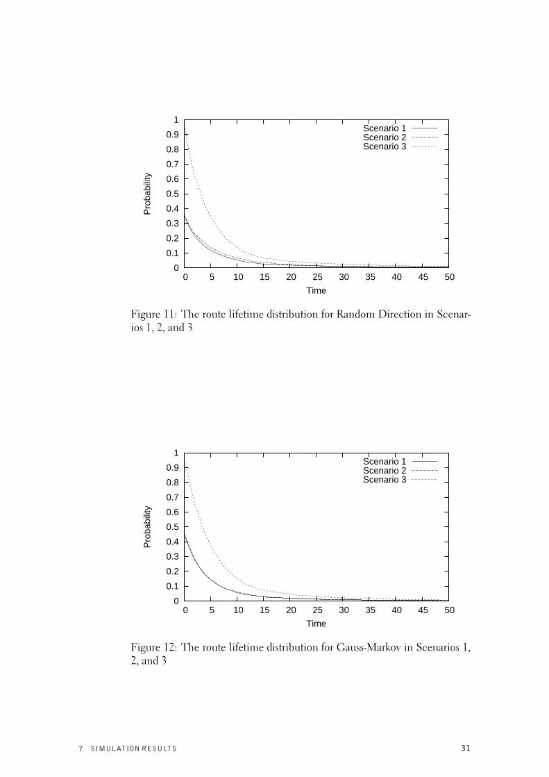
0

0.1

0.2

0.3

0.4

0.5

0.6

0.7

0.8

0.9

1

0 5 10 15 20 25 30 35 40 45 50

Pro

babi

lity

Time


Figure 11: The route lifetime distribution for Random Direction in Scenar-ios 1, 2, and 3

0

0.1

0.2

0.3

0.4

0.5

0.6

0.7

0.8

0.9

1

0 5 10 15 20 25 30 35 40 45 50

Pro

babi

lity

Time


Figure 12: The route lifetime distribution for Gauss-Markov in Scenarios 1,2, and 3


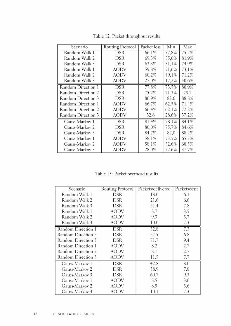
Table 12: Packet throughput results

Scenario Routing Protocol Packet loss Min MaxRandom Walk 1 DSR 66,1% 57,8% 75,2%Random Walk 2 DSR 69,3% 55,6% 81,9%Random Walk 3 DSR 63,3% 51,1% 74,9%Random Walk 1 AODV 59,8% 51,6% 73,1%Random Walk 2 AODV 60,2% 49,1% 71,2%Random Walk 3 AODV 27,0% 17,2% 50,6%

Random Direction 1 DSR 77.8% 73.5% 80.9%Random Direction 2 DSR 75.2% 71.3% 78.7Random Direction 3 DSR 86.9% 83.6 88.8%Random Direction 1 AODV 66.7% 62.5% 71.4%Random Direction 2 AODV 66.4% 62.1% 72.2%Random Direction 3 AODV 32.6 28.6% 37.2%

Gauss-Markov 1 DSR 81.4% 78.1% 84.1%Gauss-Markov 2 DSR 80,0% 75.7% 84.6%Gauss-Markov 3 DSR 84.7% 82,0 88.2%Gauss-Markov 1 AODV 58.1% 53.5% 65.3%Gauss-Markov 2 AODV 58.1% 52.6% 68.5%Gauss-Markov 3 AODV 28.0% 22.6% 37.7%

Table 13: Packet overhead results

Scenario Routing Protocol Packets/delivered Packets/sentRandom Walk 1 DSR 18.0 6.1Random Walk 2 DSR 21.6 6.6Random Walk 3 DSR 21.4 7.8Random Walk 1 AODV 8.7 3.5Random Walk 2 AODV 9.3 3.7Random Walk 3 AODV 10.0 7.3

Random Direction 1 DSR 32.8 7.3Random Direction 2 DSR 27.5 6.8Random Direction 3 DSR 71.7 9.4Random Direction 1 AODV 8.2 2.7Random Direction 2 AODV 8.1 2.7Random Direction 3 AODV 11.5 7.7

Gauss-Markov 1 DSR 42.8 8.0Gauss-Markov 2 DSR 38.9 7.8Gauss-Markov 3 DSR 60.7 9.3Gauss-Markov 1 AODV 8.5 3.6Gauss-Markov 2 AODV 8.5 3.6Gauss-Markov 3 AODV 10.1 7.3


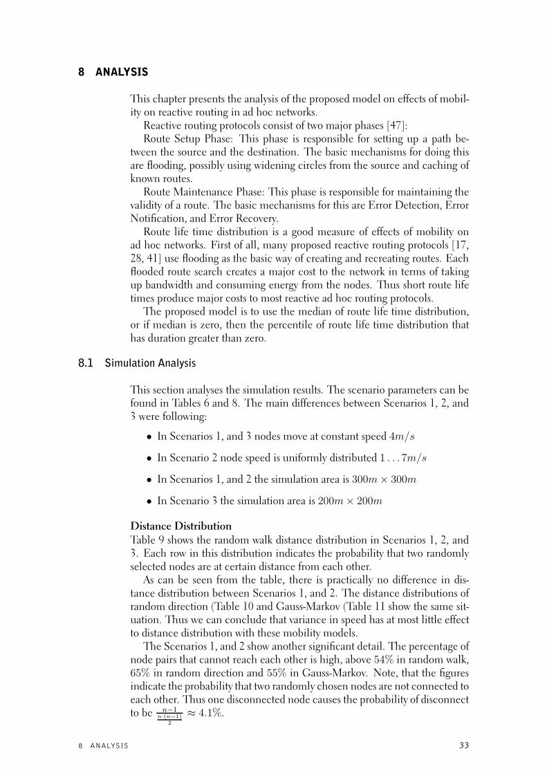
8 ANALYSIS

This chapter presents the analysis of the proposed model on effects of mobil-ity on reactive routing in ad hoc networks.

Reactive routing protocols consist of two major phases [47]:Route Setup Phase: This phase is responsible for setting up a path be-

tween the source and the destination. The basic mechanisms for doing thisare flooding, possibly using widening circles from the source and caching ofknown routes.

Route Maintenance Phase: This phase is responsible for maintaining thevalidity of a route. The basic mechanisms for this are Error Detection, ErrorNotification, and Error Recovery.

Route life time distribution is a good measure of effects of mobility onad hoc networks. First of all, many proposed reactive routing protocols [17,28, 41] use flooding as the basic way of creating and recreating routes. Eachflooded route search creates a major cost to the network in terms of takingup bandwidth and consuming energy from the nodes. Thus short route lifetimes produce major costs to most reactive ad hoc routing protocols.

The proposed model is to use the median of route life time distribution,or if median is zero, then the percentile of route life time distribution thathas duration greater than zero.

8.1 Simulation Analysis

This section analyses the simulation results. The scenario parameters can befound in Tables 6 and 8. The main differences between Scenarios 1, 2, and3 were following:

• In Scenarios 1, and 3 nodes move at constant speed 4m/s

• In Scenario 2 node speed is uniformly distributed 1 . . . 7m/s

• In Scenarios 1, and 2 the simulation area is 300m × 300m

• In Scenario 3 the simulation area is 200m × 200m

Distance DistributionTable 9 shows the random walk distance distribution in Scenarios 1, 2, and3. Each row in this distribution indicates the probability that two randomlyselected nodes are at certain distance from each other.

As can be seen from the table, there is practically no difference in dis-tance distribution between Scenarios 1, and 2. The distance distributions ofrandom direction (Table 10 and Gauss-Markov (Table 11 show the same sit-uation. Thus we can conclude that variance in speed has at most little effectto distance distribution with these mobility models.

The Scenarios 1, and 2 show another significant detail. The percentage ofnode pairs that cannot reach each other is high, above 54% in random walk,65% in random direction and 55% in Gauss-Markov. Note, that the figuresindicate the probability that two randomly chosen nodes are not connected toeach other. Thus one disconnected node causes the probability of disconnectto be n−1

n·(n−1)2

≈ 4.1%.

8 ANALYSIS 33

The probabilities in the distance distribution table for infinite distancemean that around 16 (Random Walk and Random Direction) to 21 (Gauss-Markov) nodes are unreachable from the biggest connected network. Onthe other hand, in Scenario 3 the percentage of node pairs that cannot reacheach other is between 3% (random walk and random direction) and 5%(Gauss-Markov). These percentages mean that on average in the Scenario3 one disconnected node existed.

The difference in distance distribution differs greatly in the Scenario 3,because in it the nodes are packet inside a much smaller area. The size dif-ference was exaggerated a little to make the difference in this respect clear.The reason for this is that many proposed models of how mobility affects re-active routing performance concentrate on metrics that do not take this intoaccount. The purpose of these scenarios was to clearly show the differencethat the density of the network presents.

Link Life Time Distribution

The llt distributions for random walk, random direction, and Gauss-Markovare shown in Figures 7, 8, and 9. The figures show the probability (in y-axis) that a randomly chosen link survives at least a certain time (in x-axis)for Scenarios 1, 2, and 3. Thus, the distribution is an inverted cumulativeprobability distribution of the probability that the link breaks before a givenmoment read from the x-axis.

The llt distribution is estimated using Equation 9.The results show that in random walk the link lifetimes are longest in

Scenario 3 and shortest in Scenario 2.For the random direction the results are mixed, i.e. Scenario 1 has the

lowest probability of links with life time at least in the middle range (10+seconds). It also has a tie with Scenario 3 of the probability over links withlong lifetimes (40+ seconds). On the other hand, Scenario 2 has the largestprobability of links with lifetime between 5 and 25 seconds.

The Gauss-Markov results show little difference, if any, between the threescenarios. It would seem that Scenario 1 produces slightly shorter link life-times than the other two scenarios.

Route Life Time Distribution

The rlt distributions for random walk, random direction, and Gauss-Markovare shown in Figures 10, 11, and 12. The figures show the probability (in y-axis) that the shortest route between two randomly chosen nodes survives atleast a certain time (in x-axis) for Scenarios 1, 2, and 3. Thus, the distributionis an inverted cumulative probability distribution of the probability that therout breaks before a given moment read from the x-axis.

The rlt distribution is estimated using Equation 10.The rlt distribution results for all three mobility models show that the

Scenario 3 has significantly larger route lifetimes than Scenarios 1, and 2and that Scenarios 1, and 2 are virtually indistinguishable. The reason forthe Scenario 3 producing the best route lifetimes is due to the fact that nodestend to be closer to each other in Scenario 3 than in Scenarios 1 and 2. Wecan conclude that in these scenarios the distance distribution dominates theresults.

34 8 ANALYSIS

8.2 Criterion Analysis

The purpose of this section is to examine how the model compares with theproposed criteria, i.e. clarity, predictivity and consistency.

Clarity

Intuitively, the lifetime of a route has a great effect to the reactive routingprotocols, because re-establishing a route takes time and also because it con-sumes resources such as network bandwidth and node energy.

Global flooding mechanism is such that every node broadcasts a givenpacket once, so that all connected nodes are certain to receive it. It is easyto understand that route breakages have a tremendous effect on network per-formance for a routing protocol using a basic flooding mechanism to repairroutes.

Since this is the case, most routing protocols also try to limit the amountof global flooding they do. AODV first searches the node from a distanceof 1, 3, 5, and 7 in that order and only after these have failed uses globalflooding. DSR has a mechanism for repairing routes locally. Still, both doresort to flooding protocol to discover and repair routes.

This means that the effects caused by the proposed metric are both intu-itive and easy to understand.

The model consists of two different parts, which are distance distributionand link life time distribution. They are combined to get the route life timedistribution. A human observer can look at rlt distributions (see Figures 10,11 and 12) and get a basic understanding of how mobility will affect routingprotocol performance. If more detailed analysis of the reasons for perfor-mance differences is needed, the observer may study the llt and distancedistributions (see Tables 9, 10 and 11 and Figures 7, 7, 9).

Different scenarios can also be compared using the median value of therlt distribution. This allows comparisons of different scenarios to be doneautomatically.

Predictivity

The given model gives predictions about how different mobility scenarioswill affect reactive routing protocol performance. Table 14 shows the rank-ings and rlt values for the studied scenarios. The scenario parameters aresummarized in Table 6.

The average packet loss and overhead results are reported in Tables 12 and13. The relative predicted and actual rankings are summarized in Table 15and 16. As can be seen from the tables, the throughput rankings of AODVare in line with the predictions, but the overhead rankings of AODV and therankings for DSR show no similarity between the predicted rankings and theresults from actual simulations.

One should especially note that with each mobility model, the Scenario3 should produce the best performance. But instead in DSR Gauss-Markovand random direction produce worst results in both throughput and over-head.

This means that the model does not predict results accurately. The analy-sis of the factors that affect the results in these unanticipated ways is left out

8 ANALYSIS 35

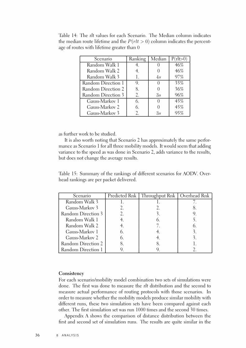
Table 14: The rlt values for each Scenario. The Median column indicatesthe median route lifetime and the P (rlt > 0) column indicates the percent-age of routes with lifetime greater than 0

Scenario Ranking Median P(rlt>0)Random Walk 1 4. 0 46%Random Walk 2 4. 0 46%Random Walk 3 1. 4s 97%

Random Direction 1 9. 0 35%Random Direction 2 8. 0 36%Random Direction 3 2. 3s 96%

Gauss-Markov 1 6. 0 45%Gauss-Markov 2 6. 0 45%Gauss-Markov 3 2. 3s 95%

as further work to be studied.It is also worth noting that Scenario 2 has approximately the same perfor-

mance as Scenario 1 for all three mobility models. It would seem that addingvariance to the speed as was done in Scenario 2, adds variance to the results,but does not change the average results.

Table 15: Summary of the rankings of different scenarios for AODV. Over-head rankings are per packet delivered.

Scenario Predicted Rnk Throughput Rnk Overhead RnkRandom Walk 3 1. 1. 7.Gauss-Markov 3 2. 2. 8.

Random Direction 3 2. 3. 9.Random Walk 1 4. 6. 5.Random Walk 2 4. 7. 6.Gauss-Markov 1 6. 4. 3.Gauss-Markov 2 6. 4. 3.

Random Direction 2 8. 8. 1.Random Direction 1 9. 9. 2.

Consistency

For each scenario/mobility model combination two sets of simulations weredone. The first was done to measure the rlt distribution and the second tomeasure actual performance of routing protocols with those scenarios. Inorder to measure whether the mobility models produce similar mobility withdifferent runs, these two simulation sets have been compared against eachother. The first simulation set was run 1000 times and the second 30 times.

Appendix A shows the comparison of distance distribution between thefirst and second set of simulation runs. The results are quite similar in the

36 8 ANALYSIS

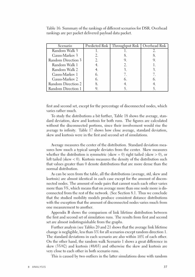
Table 16: Summary of the rankings of different scenarios for DSR. Overheadrankings are per packet delivered payload data packet.

Scenario Predicted Rnk Throughput Rnk Overhead RnkRandom Walk 3 1. 1. 2.Gauss-Markov 3 2. 8. 8.

Random Direction 3 2. 9. 9.Random Walk 1 4. 2. 1.Random Walk 2 4. 3. 3.Gauss-Markov 1 6. 7. 7.Gauss-Markov 2 6. 6. 6.

Random Direction 2 8. 4. 4.Random Direction 1 9. 5. 5.

first and second set, except for the percentage of disconnected nodes, whichvaries rather much.

To study the distributions a bit further, Table 18 shows the average, stan-dard deviation, skew and kurtosis for both runs. The figures are calculatedwithout the disconnected portions, since their involvement would rise theaverage to infinity. Table 17 shows how close average, standard deviation,skew and kurtosis were in the first and second set of simulations.

Average measures the center of the distribution. Standard deviation mea-sures how much a typical sample deviates from the center. Skew measureswhether the distribution is symmetric (skew = 0) right tailed (skew > 0), orleft tailed (skew < 0). Kurtosis measures the density of the distribution suchthat values greater than 0 denote distributions that are more dense than thenormal distribution.

As can be seen from the table, all the distributions (average, std, skew andkurtosis) are almost identical in each case except for the amount of discon-nected nodes. The amount of node pairs that cannot reach each other variesmore than 5%, which means that on average more than one node more is dis-connected from the rest of the network. (See Section 8.1. Thus we concludethat the studied mobility models produce consistent distance distributionswith the exception that the amount of disconnected nodes varies much fromone measurement to another.

Appendix B shows the comparison of link lifetime distribution betweenthe first and second set of simulation runs. The results from first and secondset are almost indistinguishable from the graphs.

Further analysis (see Tables 20 and 21 shows that the average link lifetimechange is negligible, less than 5% for all scenarios except random direction 1.The standard deviations in each scenario are also within 10% of each other.On the other hand, the random walk Scenario 1 shows a great difference inskew (35/42) and kurtosis (48/65) and otherwise the skew and kurtosis arevery close to each other in both scenario runs.

This is caused by two outliers in the latter simulations done with random

8 ANALYSIS 37

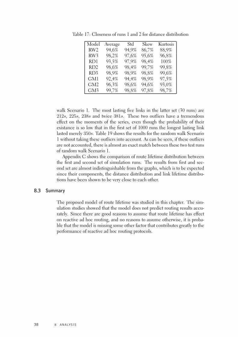
Table 17: Closeness of runs 1 and 2 for distance distribution

Model Average Std Skew KurtosisRW2 94,6% 94,9% 86,7% 88,9%RW3 98,2% 97,6% 95,6% 96,8%RD1 93,5% 97,9% 98,4% 100%RD2 98,6% 98,4% 99,7% 99,8%RD3 98,9% 98,9% 98,8% 99,6%GM1 92,4% 94,4% 98,9% 97,5%GM2 96,3% 98,6% 94,6% 93,0%GM3 99,7% 98,8% 97,8% 98,7%

walk Scenario 1. The most lasting five links in the latter set (30 runs) are212s, 225s, 238s and twice 381s. These two outliers have a tremendouseffect on the moments of the series, even though the probability of theirexistance is so low that in the first set of 1000 runs the longest lasting linklasted merely 350s. Table 19 shows the results for the random walk Scenario1 without taking these outliers into account. As can be seen, if these outliersare not accounted, there is almost an exact match between these two test runsof random walk Scenario 1.

Appendix C shows the comparison of route lifetime distribution betweenthe first and second set of simulation runs. The results from first and sec-ond set are almost indistinguishable from the graphs, which is to be expectedsince their components, the distance distribution and link lifetime distribu-tions have been shown to be very close to each other.

8.3 Summary

The proposed model of route lifetime was studied in this chapter. The sim-ulation studies showed that the model does not predict routing results accu-rately. Since there are good reasons to assume that route lifetime has effecton reactive ad hoc routing, and no reasons to assume otherwise, it is proba-ble that the model is missing some other factor that contributes greatly to theperformance of reactive ad hoc routing protocols.

38 8 ANALYSIS

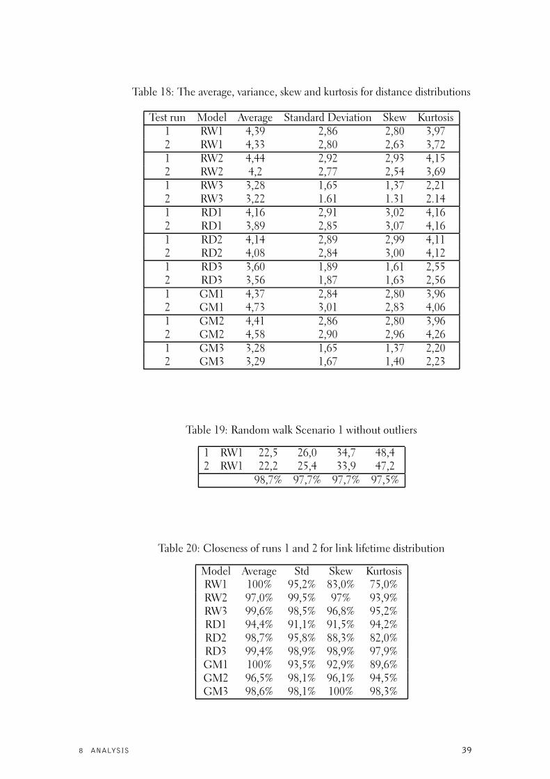
Table 18: The average, variance, skew and kurtosis for distance distributions

Test run Model Average Standard Deviation Skew Kurtosis1 RW1 4,39 2,86 2,80 3,972 RW1 4,33 2,80 2,63 3,721 RW2 4,44 2,92 2,93 4,152 RW2 4,2 2,77 2,54 3,691 RW3 3,28 1,65 1,37 2,212 RW3 3,22 1.61 1.31 2.141 RD1 4,16 2,91 3,02 4,162 RD1 3,89 2,85 3,07 4,161 RD2 4,14 2,89 2,99 4,112 RD2 4,08 2,84 3,00 4,121 RD3 3,60 1,89 1,61 2,552 RD3 3,56 1,87 1,63 2,561 GM1 4,37 2,84 2,80 3,962 GM1 4,73 3,01 2,83 4,061 GM2 4,41 2,86 2,80 3,962 GM2 4,58 2,90 2,96 4,261 GM3 3,28 1,65 1,37 2,202 GM3 3,29 1,67 1,40 2,23

Table 19: Random walk Scenario 1 without outliers

1 RW1 22,5 26,0 34,7 48,42 RW1 22,2 25,4 33,9 47,2

98,7% 97,7% 97,7% 97,5%

Table 20: Closeness of runs 1 and 2 for link lifetime distribution

Model Average Std Skew KurtosisRW1 100% 95,2% 83,0% 75,0%RW2 97,0% 99,5% 97% 93,9%RW3 99,6% 98,5% 96,8% 95,2%RD1 94,4% 91,1% 91,5% 94,2%RD2 98,7% 95,8% 88,3% 82,0%RD3 99,4% 98,9% 98,9% 97,9%GM1 100% 93,5% 92,9% 89,6%GM2 96,5% 98,1% 96,1% 94,5%GM3 98,6% 98,1% 100% 98,3%

8 ANALYSIS 39

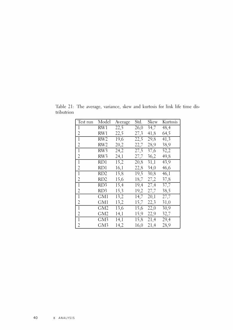
Table 21: The average, variance, skew and kurtosis for link life time dis-tributrion

Test run Model Average Std. Skew Kurtosis1 RW1 22,5 26,0 34,7 48,42 RW1 22,5 27,3 41,8 64,51 RW2 19,6 22,5 29,8 41,32 RW2 20,2 22,7 28,9 38,91 RW3 24,2 27,5 37,6 52,22 RW3 24,1 27,7 36,2 49,81 RD1 15,2 20,8 31,1 43,92 RD1 16,1 22,8 34,0 46,61 RD2 15,8 19,5 30,8 46,12 RD2 15,6 18,7 27,2 37,81 RD3 15,4 19,4 27,4 37,72 RD3 15,3 19,2 27,7 38,51 GM1 13,2 14,7 20,1 27,72 GM1 13,2 15,7 22,3 31,01 GM2 13,6 15,6 22,0 30,92 GM2 14,1 15,9 22,9 32,71 GM3 14,1 15,8 21,4 29,42 GM3 14,2 16,0 21,4 28,9

40 8 ANALYSIS

9 CONCLUSIONS

This report proposed a method for measuring the effects of mobility on re-active ad hoc routing protocols. The proposed method is to measure theexpected route life time distribution a given scenario produces.

The simulation results show that route life time distribution alone is nota good measure for problems that mobility causes to reactive ad hoc rout-ing (See Tables 14, 15 and 16). However, intuitively it should be a majorcontributor to the performance of reactive routing. This means that thereare probably other, yet unknown, variables that have a major effect on theperformance of reactive routing protocols.

The effect that is especially of notice is that DSR performed worse whenthe network was more dense, which is directly against the predictions of theproposed model. Some possible explanations for this are that collisions be-come more common, especially if no good collision prevention algorithm isin use, and network congestion caused by the large size of radio radius com-pared to simulation area. Further work on this is required to fully understandthe effects that affect protocol performance.

From these results we can predict that routing in networks with large di-ameter and dynamic links is very difficult - the route life time goes downexponentially to the number of links.

If the route lifetime distribution does have a major effect on reactive adhoc routing, it also means bad news for those who wish to use as short linksas possible to conserve energy. This is because one of the key methods forconserving node energy is to use less energy for transmissions. This, however,has two effects. First it raises the diameter of the network, and secondly makesit more likely for the existing links to have short lifetimes.

Further work is required to study the effects in more detail and to getbetter idea of how much differences in velocity and graph diameter affect therouting protocol performance.

One should also note that link life time distribution seems like a goodmetric for the effects of mobility to proactive ad hoc routing. This is becauseeach link failure creates a surge of network activity, since proactive protocolsspread the information about changed topology throughout the network.

It also suggests that for large networks with relatively stable links, proactiverouting gives better performance. Especially if link changes are mostly local.

This analysis also suggests another possibility for routing in ad hoc net-works. When distances between nodes are long, it may be a better idea toanchor the route only for certain points, or areas in the network betweensource and destination - such as clusters. This might enable the routing pro-tocol to abstract away part of the mobility that is merely local in scope.

9 CONCLUSIONS 41

ACKNOWLEDGEMENTS

This report is a reprint of my Master’s Thesis. In the course of this thesis,I have received tremendous amount of support and assistance from manypeople. I would like to express my gratitude to all those who have helpedme in this task. I want to thank my supervisor Professor Hannu H. Kari foralways having time to discuss my ideas on the subject and all the valuableadvice he has given me and my advisor Catharina Candolin who has givenme valuable input on my work. Maarit, Satu, and Tommi I wish to thank youfor your assistance.

I wish to express my gratitude to all parties that have made this thesis possi-ble by funding this research. This thesis has been funded by 007, VHO, andSamoyed projects. I am grateful for Finnish Defence Forces, TEKES andEricsson. I am especially in a debt of gratitude to Professor Pekka Orponenand Mervi Ranta for providing me with funding through past year.

42 9 CONCLUSIONS

REFERENCES

[1] A. Alwan, R. Bagrodia, N. Bambos, M. Gerla, L. Kleinrock, J. Short,and J. Villasenor. Adaptive mobile multimedia network. IEEE PersonalCommunications, 4, June 1997.

[2] R. Bagrodia and W. Liao. Maisie: A language for design of efficientdiscrete event simulation computer networks. IEEE Transactions onSoftware Engineering, April 1994.

[3] F. Bai, N. Sadagopan, and A. Helmy. Important: A framework to sys-tematically analyze the impact of mobility on performance of routingprotocols for adhoc networks. In The 22nd Annual Joint Conferenceof the IEEE Computer and Communications Societies (INFOCOM),June 2003.

[4] A. Bar-Noy, I. Kessler, and M. Sidi. Mobile users: To update or not toupdate. In Networking for Global Communications. 13th ProceedingsIEEE (INFOCOM), pages 570–576, June 1994.

[5] C. Bettstetter. Smooth is better than smart: A random mobility modelfor simulation of wireless networks. In 4th ACM Workshop on Mod-eling, Analysis and Simulation of Wireless and Mobile Systems, pages19–27, July 2001.

[6] Mobility scenario tool. See URL:http://www.cs.uni-bonn.de/IV/BonnMotion/.

[7] J. Broch, D. Maltz, D. Johnson, Y. Hu, and J. Jetcheva. A performancecomparison of multi-hop wireless ad hoc network routing protocols. In4th Annual ACM/IEEE International Conference on Mobile Comput-ing and Networking (Mobicom), pages 25–30, Dallas Texas, October1998.

[8] T. Camp, J. Boleng, and V. Davies. A survey of mobility models for adhoc network research. Wireless Communication and Mobile Comput-ing (WCMC): Special issue on Mobile Ad Hoc Networking: Research,Trends and Applications, 2:483-502, 2002.

[9] C. Chiang. Wireless network multicasting. PhD’s Thesis, University ofCalifornia, Los Angeles, 1998.

[10] C. Chiang, H. Wu, W. Liu, and M. Gerla. Routing in clustered multi-hop, mobile wireless networks with fading channel. In IEEE SingaporeInternational Conference on Networks (SICON’97), pages 197–211,April 1997.

[11] T. Cormen, C. Leiserson, and R. Rivest. Introduction to Algorithms.The MIT Electrical Engineering and Computer Science Series, 1st edi-tion, pages 514-559, 1990.

REFERENCES 43

[12] B. Dahill, K. Sanzgiri, B. Levine, E. Belding-Royer, and C. Shields. Asecure routing protocol for ad hoc networks. In International Confer-ence on Network Protocols (ICNP), November 2002.

[13] V. Davies. Evaluating mobility models within an ad hoc network. Mas-ter’s Thesis, Colorado School of Mines, 2000.

[14] M. de Berg, M. van Kreveld, M. Overmars, and O. Schwarzkopf. Com-putational Geometry: Algorithms and Applications. Springer Verlag,2000.

[15] R. Diestel. Graph Theory. Springer-Verlag, New York, USA, February2000.

[16] E. Dijkstra. A note on two problems in connexion with graphs. Nu-merische Mathematik, 1:269–271, 1959.

[17] R. Dube, C.D. Rais, K. Wang, and S.K. Tripathi. Signal stability-basedadaptive routing (ssa) for ad hoc mobile networks. IEEE Personal Com-munications, 4:36–45, February 1997.

[18] F.Bai, N. Sadagopan, and A. Helmy. Brics: A building-block approachfor analyzing routing protocols in ad hoc networks - a case study ofreactive routing protocols. In IEEE International Conference on Com-munications (ICC), June 2004.

[19] Global mobile information systems library glomosim.See URL: http://pcl.cs.ucla.edu/projects/glomosim/.

[20] C. Gui and P. Mohapatra. A self-healing and optimizing routing tech-nique for ad hoc networks. In ACM International Symposium on Mo-bile Ad Hoc Networking and Computing (MOBIHOC), 2003.

[21] R. Guérin. Channel occupancy time distribution in a cellular radiosystem. IEEE Transactions on Vehicular Technology, 36:89–99, August1987.

[22] Z. Haas. A new routing protocol for reconfigurable wireless net-works. In IEEE International Conference on Universal Communica-tions (ICUPC), pages 562–565, October 1997.

[23] D. Hong and S. Rappaport. Traffic model and performance analysisfor cellular mobile radio telephone systems with prioritized and non-prioritized handoff procedures. IEEE Transactions on Vehicular Tech-nology, VT-35:79–92, August 1986.

[24] X. Hong, M. Gerla, G. Pei, and C. Chiang. Group mobility modelfor ad hoc wireless networks. In 2nd ACM International Workshop onModeling and Simulation of Wireless and Mobile Systems (MSWiM),pages 53–60, August 1999.

[25] A. Iwata, C. Chiang, G. Pei, M. Gerla, and T. Chen. Scalable routingstrategies for ad hoc wireless networks. IEEE Journal on Selected Areasof Communications, 17:1369–1379, August 1999.

44 REFERENCES

[26] A. Jardosh, E. Belding-Royer, K. Almeroth, and S. Suri. Towards re-alistic mobility models for mobile ad hoc networks. In 9th annual in-ternational conference on Mobile computing and networking, pages217–229, September 2003.

[27] P. Johansson, T. Larsson, N. Hedman, B. Mielczarek, andM. Degermark. Scenario-based performance analysis of routing pro-tocols for mobile ad-hoc networks. In 5th Annual ACM/IEEE Interna-tional Conference on Mobile Computing and Networking (Mobicom),pages 195–206, Seattle Washington, August 1999.

[28] D. Johnson and D. Maltz. Dynamic source routing in ad hoc wirelessnetworks. In Mobile Computing, pages 153–181. Kluwer AcademicPublishers, 1996.

[29] R. Kahn, S. Gronemeyer, J. Burchfiel, and R. Kunzelman. Advancesin packet radio technology. Proceedings of the IEEE, 66, November1978.

[30] P. Krishna, N. H. Vaidya, M. Chatterjee, and D .K. Pradhan. A cluster-based approach for routing in dynamic networks. ACM SIGCOMMComputer Communication Review, pages 49–65, April 1997.

[31] B. Kwak, N. Song, and L. Miller. A canonical measure of mobility formobile ad hoc networks. In IEEE Military Communications Confer-ence (MILCOM), October 2003.

[32] B. Kwak, N. Song, and L. Miller. A mobility measure for ad-hoc net-works. IEEE Communications Letters, 7:379–381, August 2003.

[33] T. Larsson and N. Hedman. Routing protocols in wireless ad-hoc net-works - a simulation study. Master’s Thesis, Luleå Tekniska Universitet,1998.

[34] B. Liang and Z. Haas. Predictive distance-based mobility manage-ment for PCS networks. In Joint Conference of the IEEE Computerand Communications Societies, pages 1377–1384. INFOCOM, March1999.

[35] Yi-Bing Lin. Modeling techniques for large-scale PCS networks. IEEECommunications Magazine, 35:102–115, February 1997.

[36] J. Markoulidakis, G. Lyberopoulos, D. Tsirkas, and E. Sykas. Mobil-ity modeling in third-generation mobile telecommunications systems.IEEE Personal Communications, 4:41–56, August 1997.

[37] S. Murthy and J. Garcia-Luna-Aceves. An efficient routing protocol forwireless networks. Mobile Networks and Applications, 1(2):183–197,October 1996.

[38] The network simulator - ns-2.See URL: http://www.isi.edu/nsnam/ns/, 2002.

REFERENCES 45

[39] V. Park and M. Corson. A highly adaptive distributed routing algorithmfor mobile wireless networks. In Sixteenth Annual Joint Conference ofthe IEEE Computer and Communications Societies (INFOCOM’97)(3), pages 1405–1413, April 1997.

[40] G. Pei, M. Gerla, X. Hong, and C. Chiang. A wireless hierarchicalrouting protocol with group mobility. In Wireless Communications andNetworking Conference (IEEE WCNC’99), pages 1538-1542, Septem-ber 1999.

[41] C. Perkins. Ad-hoc on-demand distance vector routing. In Sec-ond IEEE Workshop on Mobile Computing Systems and Applications(WMCSA ’99), pages 90-100, February 1999.

[42] C. Perkins and P. Bhagwat. Highly dynamic destination-sequenceddistance-vector routing (dsdv) for mobile computers. In ACM SIG-COMM Conference on Communications Architectures, Protocols andApplications, pages 234–244, August 1994.

[43] E. Del Re, R. Fantacci, and G. Giambene. Handover and dynamicchannel allocation techniques in mobile cellular networks. IEEETransactions in Vehicular Technology, 44:229–237, May 1995.

[44] C. Rosee and R. Yaters. Location uncertainty in mobile networks: Atheoretical framcework. IEEE Communications Magazine, 35:94–101,February 1997.

[45] E. Royer, P. Melliar-Smith, and L. Moser. An analysis of optimum nodedensity for ad hoc mobile networks. In IEEE International Conferenceon Communications (ICC), 2001.

[46] E. Royer and C. Toh. A review of current routing protocols for ad hocmobile wireless networks. IEEE Personal Communications, pages 46–55, April 1999.

[47] N. Sadagopan, F. Bai, B. Krishnamachari, and A. Helmy. Paths: Analy-sis of path duration statistics and their impact on reactive manet routingprotocols. In 4th ACM international symposium on Mobile ad hoc net-working & computing, pages 245–256. ACM Press, June 2003.

[48] M. Sanchez. Mobility models.See URL: http://www.disca.upv.es/misan/mobmodel.htm, 2001.

[49] D. Tan, S. Zhou, J. Ho, J. Mehta, and H. Tanabe. Design and eval-uation of an individually simulated mobility model in wireless ad hocnetworks. In Communication Networks and Distributed Systems Mod-eling and Simulation Conference 2002, San Antonio, TX, 2002.

[50] D. Turgut, S. Das, and M. Chatterjee. Longevity of routes in mobilead hoc networks. In Vehicular Technology Conference Volume 4, 6-9,pages 2833–2837. Spring. IEEE VTS 53rd, May 2001.

46 REFERENCES

[51] M. Zonoosi and P. Dassanayake. User mobility modeling and char-acterisation of mobility patterns. IEEE Journal on Selected Areas inCommunications, 15:1239–1252, September 1997.

REFERENCES 47

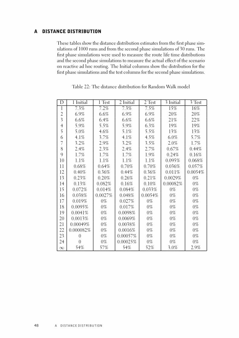
A DISTANCE DISTRIBUTION

These tables show the distance distribution estimates from the first phase sim-ulations of 1000 runs and from the second phase simulations of 30 runs. Thefirst phase simulations were used to measure the route life time distributionsand the second phase simulations to measure the actual effect of the scenarioon reactive ad hoc routing. The Initial columns show the distribution for thefirst phase simulations and the test columns for the second phase simulations.

Table 22: The distance distribution for Random Walk model

D 1 Initial 1 Test 2 Initial 2 Test 3 Initial 3 Test1 7.3% 7.2% 7.3% 7.5% 15% 16%2 6.9% 6.6% 6.9% 6.9% 20% 20%3 6.6% 6.4% 6.6% 6.6% 21% 22%4 5.9% 5.5% 5.9% 6.3% 19% 19%5 5.0% 4.6% 5.1% 5.5% 13% 13%6 4.1% 3.7% 4.1% 4.5% 6.0% 5.7%7 3.2% 2.9% 3.2% 3.5% 2.0% 1.7%8 2.4% 2.3% 2.4% 2.7% 0.67% 0.44%9 1.7% 1.7% 1.7% 1.9% 0.24% 0.16%

10 1.1% 1.1% 1.1% 1.1% 0.095% 0.068%11 0.68% 0.64% 0.70% 0.70% 0.036% 0.057%12 0.40% 0.36% 0.44% 0.36% 0.011% 0.0054%13 0.23% 0.20% 0.26% 0.21% 0.0029% 0%14 0.13% 0.082% 0.16% 0.10% 0.00082% 0%15 0.072% 0.014% 0.084% 0.033% 0% 0%16 0.038% 0.0027% 0.048% 0.0054% 0% 0%17 0.019% 0% 0.027% 0% 0% 0%18 0.0095% 0% 0.017% 0% 0% 0%19 0.0041% 0% 0.0098% 0% 0% 0%20 0.0013% 0% 0.0069% 0% 0% 0%21 0.00049% 0% 0.0038% 0% 0% 0%22 0.000082% 0% 0.0016% 0% 0% 0%23 0 0% 0.00057% 0% 0% 0%24 0 0% 0.00025% 0% 0% 0%∞ 54% 57% 54% 52% 3.0% 2.9%

48 A DISTANCE DISTRIBUTION

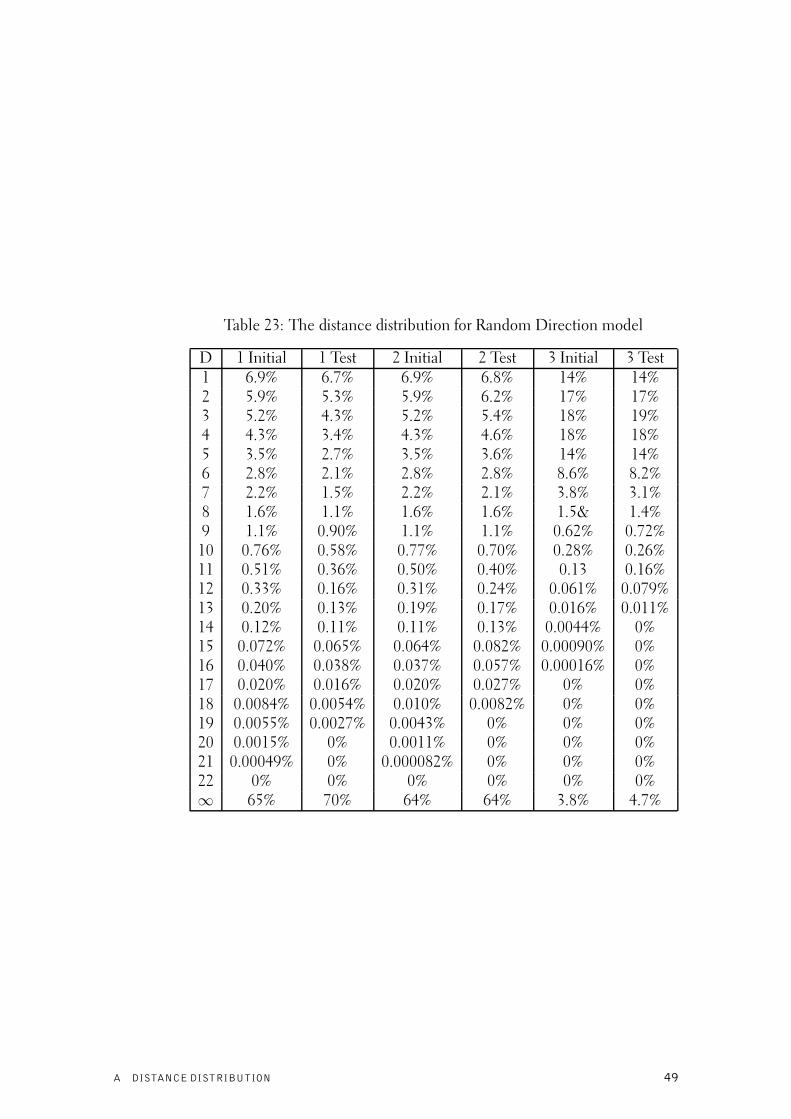
Table 23: The distance distribution for Random Direction model

D 1 Initial 1 Test 2 Initial 2 Test 3 Initial 3 Test1 6.9% 6.7% 6.9% 6.8% 14% 14%2 5.9% 5.3% 5.9% 6.2% 17% 17%3 5.2% 4.3% 5.2% 5.4% 18% 19%4 4.3% 3.4% 4.3% 4.6% 18% 18%5 3.5% 2.7% 3.5% 3.6% 14% 14%6 2.8% 2.1% 2.8% 2.8% 8.6% 8.2%7 2.2% 1.5% 2.2% 2.1% 3.8% 3.1%8 1.6% 1.1% 1.6% 1.6% 1.5& 1.4%9 1.1% 0.90% 1.1% 1.1% 0.62% 0.72%

10 0.76% 0.58% 0.77% 0.70% 0.28% 0.26%11 0.51% 0.36% 0.50% 0.40% 0.13 0.16%12 0.33% 0.16% 0.31% 0.24% 0.061% 0.079%13 0.20% 0.13% 0.19% 0.17% 0.016% 0.011%14 0.12% 0.11% 0.11% 0.13% 0.0044% 0%15 0.072% 0.065% 0.064% 0.082% 0.00090% 0%16 0.040% 0.038% 0.037% 0.057% 0.00016% 0%17 0.020% 0.016% 0.020% 0.027% 0% 0%18 0.0084% 0.0054% 0.010% 0.0082% 0% 0%19 0.0055% 0.0027% 0.0043% 0% 0% 0%20 0.0015% 0% 0.0011% 0% 0% 0%21 0.00049% 0% 0.000082% 0% 0% 0%22 0% 0% 0% 0% 0% 0%∞ 65% 70% 64% 64% 3.8% 4.7%

A DISTANCE DISTRIBUTION 49

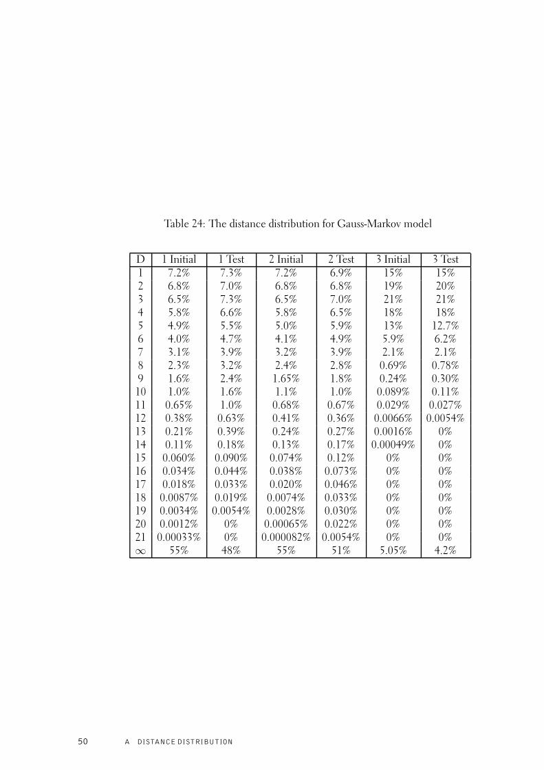
Table 24: The distance distribution for Gauss-Markov model

D 1 Initial 1 Test 2 Initial 2 Test 3 Initial 3 Test1 7.2% 7.3% 7.2% 6.9% 15% 15%2 6.8% 7.0% 6.8% 6.8% 19% 20%3 6.5% 7.3% 6.5% 7.0% 21% 21%4 5.8% 6.6% 5.8% 6.5% 18% 18%5 4.9% 5.5% 5.0% 5.9% 13% 12.7%6 4.0% 4.7% 4.1% 4.9% 5.9% 6.2%7 3.1% 3.9% 3.2% 3.9% 2.1% 2.1%8 2.3% 3.2% 2.4% 2.8% 0.69% 0.78%9 1.6% 2.4% 1.65% 1.8% 0.24% 0.30%

10 1.0% 1.6% 1.1% 1.0% 0.089% 0.11%11 0.65% 1.0% 0.68% 0.67% 0.029% 0.027%12 0.38% 0.63% 0.41% 0.36% 0.0066% 0.0054%13 0.21% 0.39% 0.24% 0.27% 0.0016% 0%14 0.11% 0.18% 0.13% 0.17% 0.00049% 0%15 0.060% 0.090% 0.074% 0.12% 0% 0%16 0.034% 0.044% 0.038% 0.073% 0% 0%17 0.018% 0.033% 0.020% 0.046% 0% 0%18 0.0087% 0.019% 0.0074% 0.033% 0% 0%19 0.0034% 0.0054% 0.0028% 0.030% 0% 0%20 0.0012% 0% 0.00065% 0.022% 0% 0%21 0.00033% 0% 0.000082% 0.0054% 0% 0%∞ 55% 48% 55% 51% 5.05% 4.2%

50 A DISTANCE DISTRIBUTION

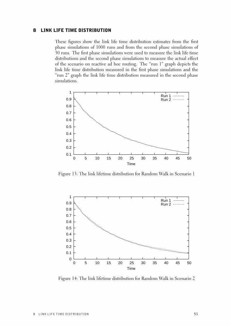
B LINK LIFE TIME DISTRIBUTION

These figures show the link life time distribution estimates from the firstphase simulations of 1000 runs and from the second phase simulations of30 runs. The first phase simulations were used to measure the link life timedistributions and the second phase simulations to measure the actual effectof the scenario on reactive ad hoc routing. The “run 1” graph depicts thelink life time distribution measured in the first phase simulations and the“run 2” graph the link life time distribution measured in the second phasesimulations.

0.1

0.2

0.3

0.4

0.5

0.6

0.7

0.8

0.9

1

0 5 10 15 20 25 30 35 40 45 50

Time

Run 1Run 2

Figure 13: The link lifetime distribution for Random Walk in Scenario 1

0

0.1

0.2

0.3

0.4

0.5

0.6

0.7

0.8

0.9

1

0 5 10 15 20 25 30 35 40 45 50

Time

Run 1Run 2


B LINK LIFE TIME DISTRIBUTION 51

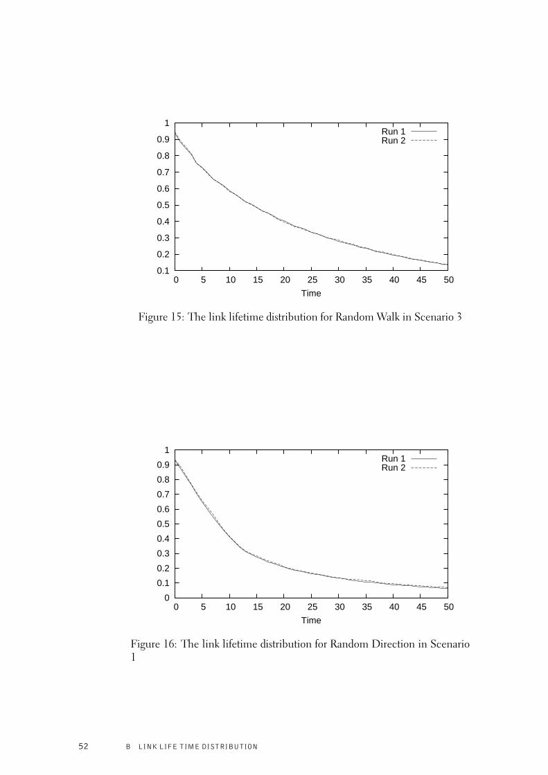
0.1

0.2

0.3

0.4

0.5

0.6

0.7

0.8

0.9

1

0 5 10 15 20 25 30 35 40 45 50

Time

Run 1Run 2


0

0.1

0.2

0.3

0.4

0.5

0.6

0.7

0.8

0.9

1

0 5 10 15 20 25 30 35 40 45 50

Time

Run 1Run 2

Figure 16: The link lifetime distribution for Random Direction in Scenario1

52 B LINK LIFE TIME DISTRIBUTION

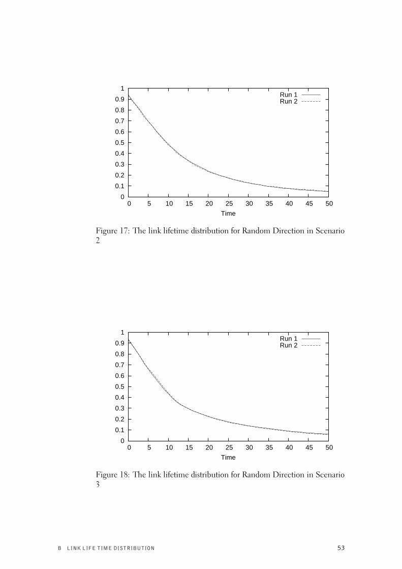
0

0.1

0.2

0.3

0.4

0.5

0.6

0.7

0.8

0.9

1

0 5 10 15 20 25 30 35 40 45 50

Time

Run 1Run 2


0

0.1

0.2

0.3

0.4

0.5

0.6

0.7

0.8

0.9

1

0 5 10 15 20 25 30 35 40 45 50

Time

Run 1Run 2



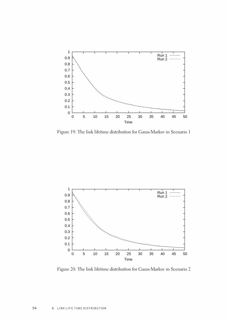
0

0.1

0.2

0.3

0.4

0.5

0.6

0.7

0.8

0.9

1

0 5 10 15 20 25 30 35 40 45 50

Time

Run 1Run 2

Figure 19: The link lifetime distribution for Gauss-Markov in Scenario 1

0

0.1

0.2

0.3

0.4

0.5

0.6

0.7

0.8

0.9

1

0 5 10 15 20 25 30 35 40 45 50

Time

Run 1Run 2


54 B LINK LIFE TIME DISTRIBUTION

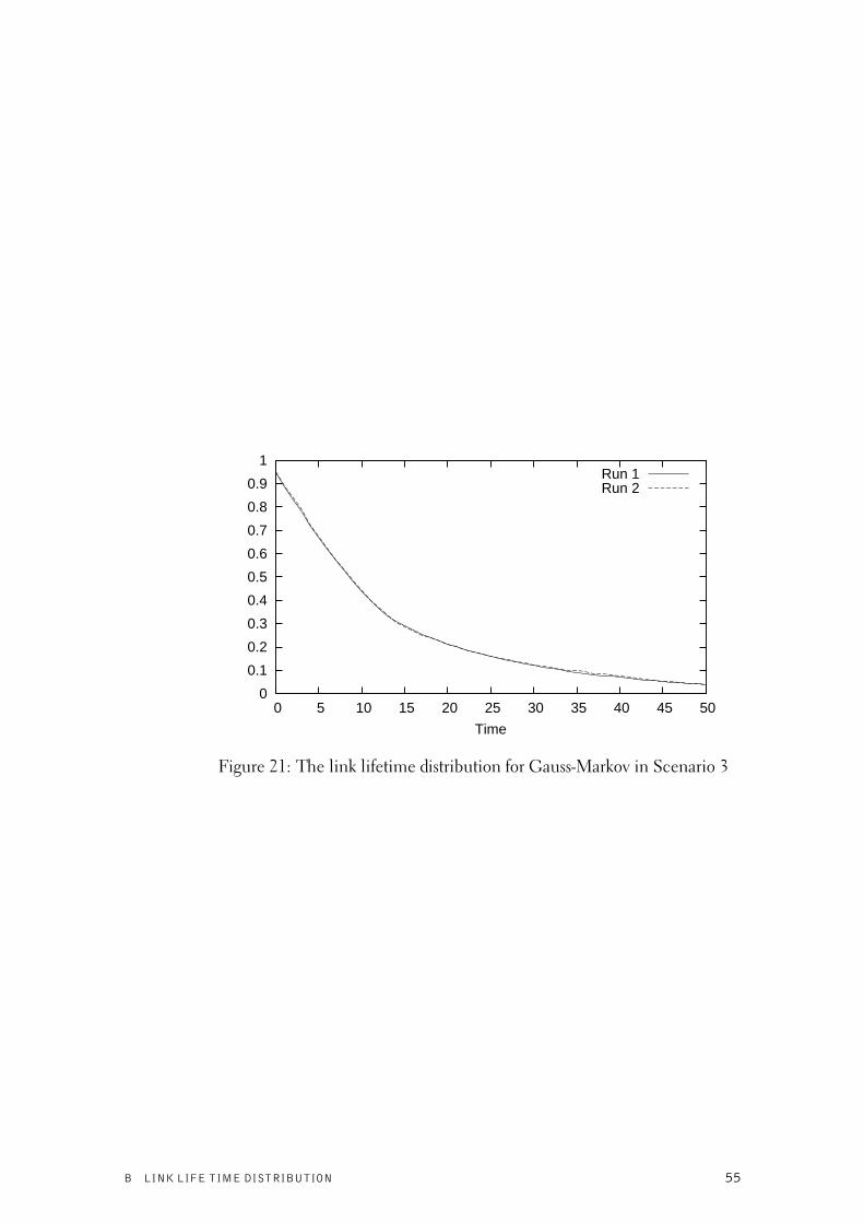
0

0.1

0.2

0.3

0.4

0.5

0.6

0.7

0.8

0.9

1

0 5 10 15 20 25 30 35 40 45 50

Time

Run 1Run 2



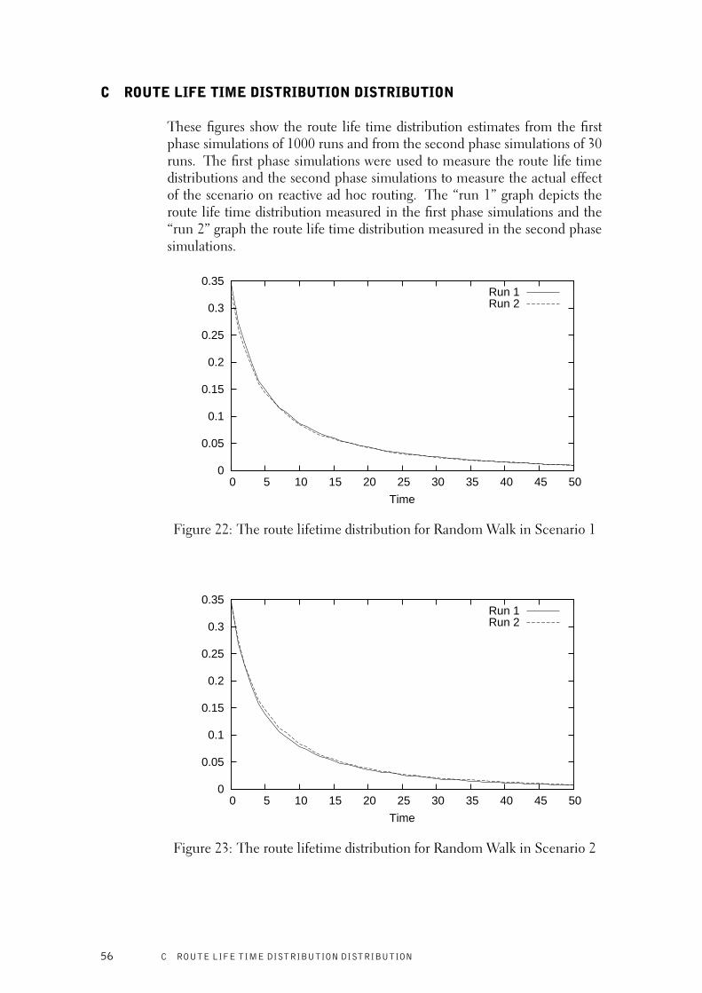
C ROUTE LIFE TIME DISTRIBUTION DISTRIBUTION

These figures show the route life time distribution estimates from the firstphase simulations of 1000 runs and from the second phase simulations of 30runs. The first phase simulations were used to measure the route life timedistributions and the second phase simulations to measure the actual effectof the scenario on reactive ad hoc routing. The “run 1” graph depicts theroute life time distribution measured in the first phase simulations and the“run 2” graph the route life time distribution measured in the second phasesimulations.

0

0.05

0.1

0.15

0.2

0.25

0.3

0.35

0 5 10 15 20 25 30 35 40 45 50

Time

Run 1Run 2

Figure 22: The route lifetime distribution for Random Walk in Scenario 1

0

0.05

0.1

0.15

0.2

0.25

0.3

0.35

0 5 10 15 20 25 30 35 40 45 50

Time

Run 1Run 2


56 C ROUTE LIFE TIME DISTRIBUTION DISTRIBUTION

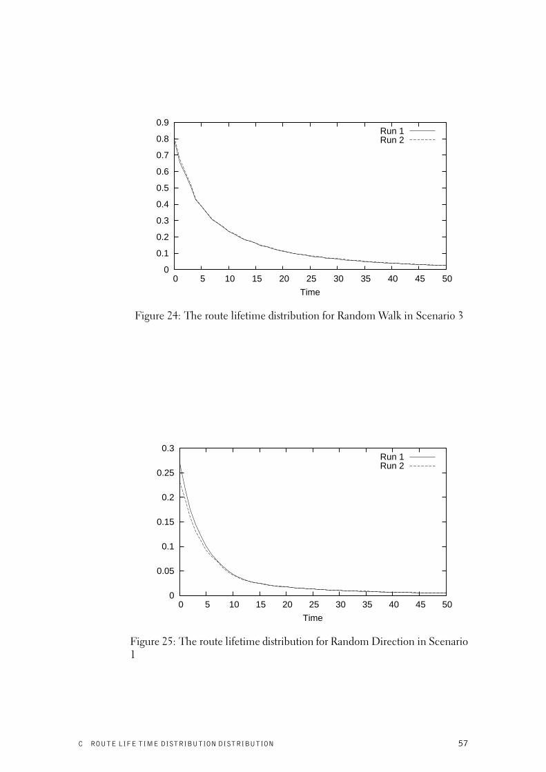
0

0.1

0.2

0.3

0.4

0.5

0.6

0.7

0.8

0.9

0 5 10 15 20 25 30 35 40 45 50

Time

Run 1Run 2


0

0.05

0.1

0.15

0.2

0.25

0.3

0 5 10 15 20 25 30 35 40 45 50

Time

Run 1Run 2

Figure 25: The route lifetime distribution for Random Direction in Scenario1

C ROUTE LIFE TIME DISTRIBUTION DISTRIBUTION 57

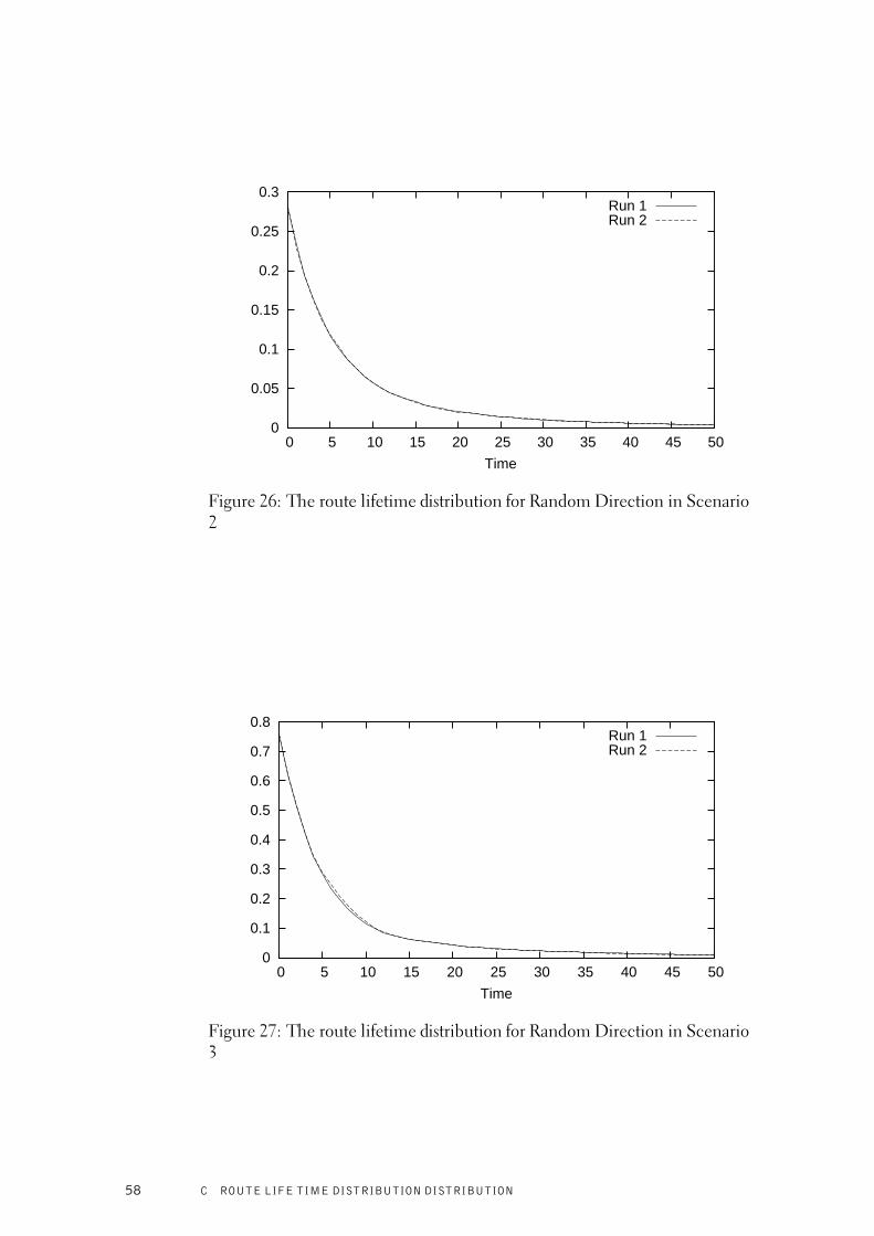
0

0.05

0.1

0.15

0.2

0.25

0.3

0 5 10 15 20 25 30 35 40 45 50

Time

Run 1Run 2


0

0.1

0.2

0.3

0.4

0.5

0.6

0.7

0.8

0 5 10 15 20 25 30 35 40 45 50

Time

Run 1Run 2



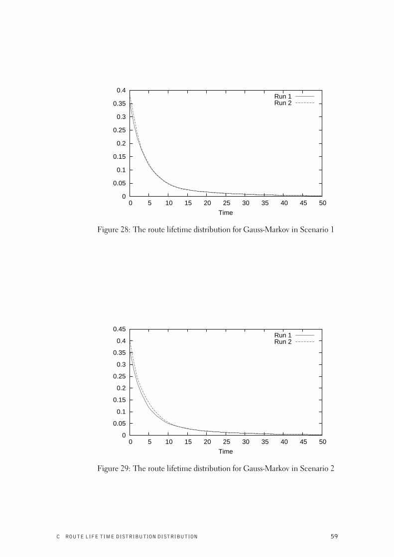
0

0.05

0.1

0.15

0.2

0.25

0.3

0.35

0.4

0 5 10 15 20 25 30 35 40 45 50

Time

Run 1Run 2

Figure 28: The route lifetime distribution for Gauss-Markov in Scenario 1

0

0.05

0.1

0.15

0.2

0.25

0.3

0.35

0.4

0.45

0 5 10 15 20 25 30 35 40 45 50

Time

Run 1Run 2


C ROUTE LIFE TIME DISTRIBUTION DISTRIBUTION 59

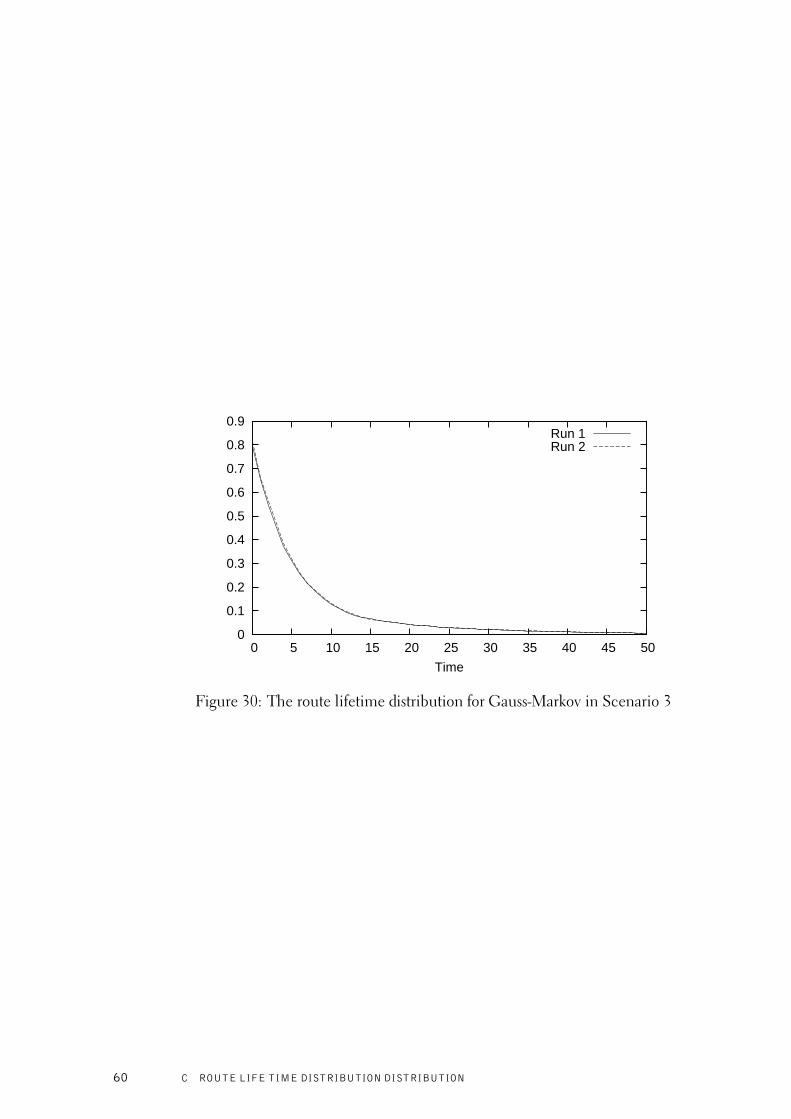
0

0.1

0.2

0.3

0.4

0.5

0.6

0.7

0.8

0.9

0 5 10 15 20 25 30 35 40 45 50

Time

Run 1Run 2



HELSINKI UNIVERSITY OF TECHNOLOGY LABORATORY FOR THEORETICAL COMPUTER SCIENCE

RESEARCH REPORTS

HUT-TCS-A78 Petteri Kaski

A Census of Steiner Triple Systems and Some Related Combinatorial Objects. June 2003.

HUT-TCS-A79 Heikki Tauriainen

Nested Emptiness Search for Generalized Buchi Automata. July 2003.

HUT-TCS-A80 Tommi Junttila

On the Symmetry Reduction Method for Petri Nets and Similar Formalisms.

September 2003.

HUT-TCS-A81 Marko Makela

Efficient Computer-Aided Verification of Parallel and Distributed Software Systems.

November 2003.

HUT-TCS-A82 Tomi Janhunen

Translatability and Intranslatability Results for Certain Classes of Logic Programs.

November 2003.

HUT-TCS-A83 Heikki Tauriainen

On Translating Linear Temporal Logic into Alternating and Nondeterministic Automata.

December 2003.

HUT-TCS-A84 Johan Wallen

On the Differential and Linear Properties of Addition. December 2003.

HUT-TCS-A85 Emilia Oikarinen

Testing the Equivalence of Disjunctive Logic Programs. December 2003.

HUT-TCS-A86 Tommi Syrjanen

Logic Programming with Cardinality Constraints. December 2003.

HUT-TCS-A87 Harri Haanpaa, Patric R. J. Ostergard

Sets in Abelian Groups with Distinct Sums of Pairs. February 2004.

HUT-TCS-A88 Harri Haanpaa

Minimum Sum and Difference Covers of Abelian Groups. February 2004.

HUT-TCS-A89 Harri Haanpaa

Constructing Certain Combinatorial Structures by Computational Methods. February 2004.

HUT-TCS-A90 Matti Jarvisalo

Proof Complexity of Cut-Based Tableaux for Boolean Circuit Satisfiability Checking.

March 2004.

HUT-TCS-A91 Mikko Sarela

Measuring the Effects of Mobility on Reactive Ad Hoc Routing Protocols. May 2004.

ISBN 951-22-7145-1

ISSN 1457-7615

MEASURING THE EFFECTS OF MOBILITY ON REACTIVE … · MEASURING THE EFFECTS OF MOBILITY ON REACTIVE...

Documents

Transcript of MEASURING THE EFFECTS OF MOBILITY ON REACTIVE … · MEASURING THE EFFECTS OF MOBILITY ON REACTIVE...