Measuring Text Readability by Lexical Relations Retrieved ...
243
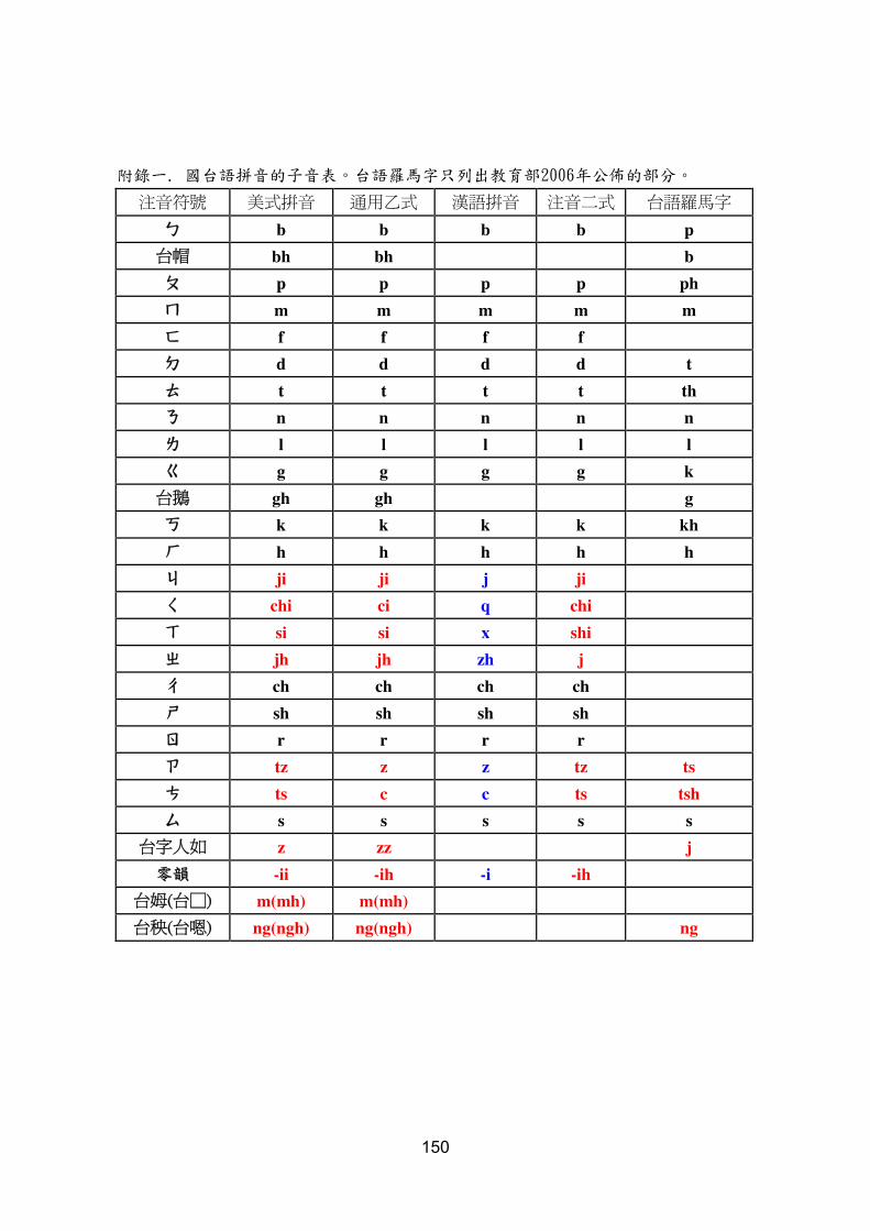
Measuring Text Readability by Lexical Relations Retrieved from WordNet Shu-yen Lin, Cheng-chao Su, Yu-da Lai, Li-chin Yang, Shu-kai Hsieh English Department National Taiwan Normal University [email protected] Abstract Current readability formulae have often been criticized for being unstable or not valid. They are mostly computed in regression analysis based on intuitively-chosen variables and graded readings. This study explores the relation between text readability and the conceptual categories proposed in Prototype Theory. These categories form a hierarchy: Basic level words like guitar represent the objects humans interact with most readily. They are acquired by children earlier than their superordinate words (or hypernyms) like stringed instrument and their subordinate words (or hyponyms) like acoustic guitar. Therefore, the readability of a text is presumably associated with the ratio of basic level words it contains. WordNet, a network of meaningfully related words, provides the best online open source database for studying such lexical relations. Our preliminary studies show that a basic level word can be identified by its frequency to form compounds (e.g. chair Æ armchair) and the length difference from its hyponyms in average. We compared selected high school English textbook readings in terms of their basic level word ratios and their values calculated in several readability formulae. Basic level word ratios turned out to be the only one positively correlated with the text levels. Keywords: Readability, Ontology, Prototype Theory, WordNet, Basic Level Word 1. Introduction Reading process is the core of language education. Teachers now have access to a vast amount of texts extractable from the Internet inter alia, but the materials thus found are rarely classified according to comprehension difficulty. It is not uncommon to see foreign language teachers using texts not compatible with the students’ reading abilities. Traditional methods of measuring text readability typically rely on the counting of sentences, words, syllables, or characters. However, these formulae have been criticized for being unstable and incapable of providing deeper information about the text. Recently, the focus of readability formula formation has shifted to the search for meaningful predictors and stronger association between the variables and the comprehension difficulty. We start our research by assuming in line with Rosch et al.’s Prototype Theory [1] that words form conceptual hierarchies in that words at different hierarchical levels pose different processing difficulties. This processing difficulty is presumably correlated with the reading difficulty of the text containing the words. Putting the logic into templates, the measurement 1
Transcript of Measuring Text Readability by Lexical Relations Retrieved ...

Measuring Text Readability by Lexical Relations
Retrieved from WordNet
Shu-yen Lin Cheng-chao Su Yu-da Lai Li-chin Yang Shu-kai Hsieh English Department
National Taiwan Normal University sylinntnuedutw
Abstract
Current readability formulae have often been criticized for being unstable or not valid They are mostly computed in regression analysis based on intuitively-chosen variables and graded readings This study explores the relation between text readability and the conceptual categories proposed in Prototype Theory These categories form a hierarchy Basic level words like guitar represent the objects humans interact with most readily They are acquired by children earlier than their superordinate words (or hypernyms) like stringed instrument and their subordinate words (or hyponyms) like acoustic guitar Therefore the readability of a text is presumably associated with the ratio of basic level words it contains WordNet a network of meaningfully related words provides the best online open source database for studying such lexical relations Our preliminary studies show that a basic level word can be identified by its frequency to form compounds (eg chair armchair) and the length difference from its hyponyms in average We compared selected high school English textbook readings in terms of their basic level word ratios and their values calculated in several readability formulae Basic level word ratios turned out to be the only one positively correlated with the text levels Keywords Readability Ontology Prototype Theory WordNet Basic Level Word 1 Introduction
Reading process is the core of language education Teachers now have access to a vast amount of texts extractable from the Internet inter alia but the materials thus found are rarely classified according to comprehension difficulty It is not uncommon to see foreign language teachers using texts not compatible with the studentsrsquo reading abilities Traditional methods of measuring text readability typically rely on the counting of sentences words syllables or characters However these formulae have been criticized for being unstable and incapable of providing deeper information about the text Recently the focus of readability formula formation has shifted to the search for meaningful predictors and stronger association between the variables and the comprehension difficulty
We start our research by assuming in line with Rosch et alrsquos Prototype Theory [1] that words form conceptual hierarchies in that words at different hierarchical levels pose different processing difficulties This processing difficulty is presumably correlated with the reading difficulty of the text containing the words Putting the logic into templates the measurement
1
of text readability can be done by calculating the average hierarchical levels at which the words of a text fall
Our study comprises two stages In the preliminary experiments we utilized WordNet [2] an online lexical database of English to identify basic level words In the subsequent experiment we compared selected readings in terms of their basic level word ratios and their values calculated in several readability formulae Basic level word ratios turned out to be the only one positively correlated with the text levels
The remainder of this paper is organized as follows Section 2 reviews the common indices the traditional readability formulae are based on and the criticism they have received In Section 3 we first review an approach that centers on ontology structure and then propose our own ontology-based approach Section 4 is about methodology ndash how to identify basic level words and how to assess the validity of our method against other readability formulae Section 5 reports the results of the assessment and discusses the strength and weaknesses of our approach In this section we also suggest what can be done in further research 2 Literature Review
In this section we first summarize the indices of the traditional readability formulae and then give an account of the criticism these formulae face 21 Indices of Readability ndash Vocabulary Syntactic and Semantic Complexity
The earliest work on readability measurement goes back to Thorndike [3] where word frequency in corpus is considered an important index This is based on the assumption that the more frequent a word is used the easier it should be Followers of this logic have compiled word lists that include either often-used or seldom-used words whose presence or absence is assumed to be able to determine vocabulary complexity thus text complexity Vocabulary complexity is otherwise measured in terms of word length eg the Flesch formula [4] and FOG formula [5] This is based on another assumption that the longer a word is the more difficult it is to comprehend [6] Many readability formulae presume the correlation between comprehension difficulty and syntactic complexity For Dale and Chall [7] Flesch formula [4] and FOG index [5] syntactic complexity boils down to the average length of sentences in a text Heilman Collins-Thompson Callan and Eskenazi [8] also take morphological features as a readability index for morphosyntactically rich languages Das amp Roychoudhuryrsquos readability index [9] for Bangla has two variables average sentence length and number of syllables per word Flesch [4] and Cohen [10] take semantic factors into account by counting the abstract words of a text Kintsch [11] focuses on propositional density and inferences Wiener M Rubano M and Shilkret R [12] propose a scale based on ten categories of semantic
2
relations including eg temporal ordering and causality They show that the utterances of fourth- sixth- and eighth-grade children can be differentiated on their semantic density scale Since 1920 more than fifty readability formulae have been proposed in the hope of providing tools to measure readability more accurately and efficaciously [13] Nonetheless it is not surprising to see criticism over these formulae given that reading is a complex process 22 Criticism of the Traditional Readability Formulae
One type of criticism questions the link between readability and word lists Bailin and Grafstein [14] argue that the validity of such a link is based on the prerequisite that words in a language remain relatively stable However different socio-cultural groups have different core vocabularies and rapid cultural change makes many words out of fashion The authors also question the validity of measuring vocabulary complexity by word length showing that many mono- or bi-syllabic words are actually more unfamiliar than longer polysyllabic terms
These authors also point out the flaw of a simple equation between syntactic complexity and sentence length by giving the sample sentences as follows (1) I couldnrsquot answer your e-mail There was a power outage (2) I couldnrsquot answer your e-mail because there was a power outage (2) is longer than (1) thus computed as more difficult but the subordinator ldquobecauserdquo which explicitly links the authorrsquos inability to e-mail to the power outage actually aids the comprehension The longer passage is accordingly easier than the shorter one
Hua and Wang [15] point out that researchers typically select as the criterion passages standard graded texts whose readability has been agreed upon They then try to sort out the factors that may affect the readability of these texts Regression analyses are used to determine the independent variables and the parameters of the variables However the researchers have no proof of the cause-effect relation between the selected independent variables and the dependent variable ie readability
Challenge to the formula formation is also directed at the selection of criterion passages Schriver [16] argue that readability formulae are inherently unreliable because they depend on criterion passages too short to reflect cohesiveness too varied to support between-formula comparisons and too text-oriented to account for the effects of lists enumerated sequences and tables on text comprehension
The problems of the traditional readability formulae beg for re-examination of the correlation between the indices and the readability they are supposed to reflect 3 Ontology-based Approach to Readability Measurement
31 An ontology-based method of retrieving information
Yan X Li X and Song D [17] propose a domain-ontology method to rank documents on
3
the generality (or specificity) scale A document is more specific if it has broaderdeeper Document Scope (DS) andor tighter Document Cohesion (DC) DS refers to a collection of terms that are matched with the query in a specific domain If the concepts thus matched are associated with one another more closely then DC is tighter The authors in their subsequent study [18] apply DS and DC to compute text readability in domain specific documents and are able to perform better prediction than the traditional readability formulae In what follows we describe the approach we take in this study which is similar in spirit to Yan et alrsquos [18] method 32 An Ontology-based Approach to the Study of Lexical Relations
In this small-scaled study we focus on lexical complexity (or simplicity) of the words in a text and adopt Rosch et alrsquos Prototype Theory [1] 321 Prototype Theory
According to Prototype Theory our conceptual categorization exhibits a three-leveled hierarchy basic levels superordinate levels and subordinate levels Imagine an everyday conversation setting where a person says ldquoWho owns this pianordquo the naming of an object with lsquopianorsquo will not strike us as noteworthy until the alternative ldquoWho owns this string instrumentrdquo is brought to our attention Both terms are truth-conditionally adequate but only the former is normally used The word lsquopianorsquo conveys a basic level category while lsquostring instrumentrsquo is a superordinate category Suppose the piano in our example is of the large expensive type ie a grand piano we expect a subordinate category word to be used in eg ldquoWho owns this grand pianordquo only when the differentiation between different types of pianos is necessary Basic level is the privileged level in the hierarchy of categorical conceptualization Developmentally they are acquired earlier by children than their superordinate and subordinate words Conceptually basic level category represents the concepts humans interact with most readily A picture of an apple is easy to draw while drawing a fruit would be difficult and drawing a crab apple requires expertise knowledge Informatively basic level category contains a bundle of co-occurring features ndash an apple has reddish or greenish skin white pulp and a round shape while it is hard to pinpoint the features of lsquofruitrsquo and for a layman hardly any significant features can be added to lsquocrab applersquo Applying the hierarchical structure of conceptual categorization to lexical relations we assume that a basic level word is easier for the reader than its superordinate and subordinate words and one text should be easier than another if it contains more basic level words
4
322 WordNet ndash An Ontology-Based Lexical Database of English
WordNet [2] is a large online lexical database of English The words are interlinked by means of conceptual-semantic and lexical relations It can be used as a lexical ontology in computational linguistics Its underlying design principle has much in common with the hierarchical structure proposed in Prototype Theory illustrated in 321 In the vertical dimension the hypernymhyponym relationships among the nouns can be interpreted as hierarchical relations between conceptual categories The direct hypernym of lsquoapplersquo is lsquoedible fruitrsquo One of the direct hyponyms of lsquoapplersquo is lsquocrab applersquo Note however hypernyms and hyponyms are relativized notions in WordNet The word lsquocrab applersquo for instance is also a hypernym in relation to lsquoSiberian crab applersquo An ontological tree may well exceed three levels No tags in WordNet tell us which nouns fall into the basic level category defined in Prototype Theory In the next section we try to retrieve these nouns 4 Methodology
41 Experiment 1
We examined twenty basic level words identified by Rosch et al [1] checking the word length and lexical complexity of these basic level words and their direct hypernyms as well as direct hyponyms in WordNet [2] A basic level word is assumed to have these features (1) It is relatively short (containing less letters than their hypernymshyponyms in average) (2) Its direct hyponyms have more synsets1 than its direct hypernyms (3) It is morphologically simple Notice that some entries in WordNet [2] contain more than one word We assume that an item composed of two or more words is NOT a basic level word A lexical entry composed of two or more words is defined as a COMPOUND in this study The first word of a compound may or may not be a noun and there may or may not be spaces or hyphens between the component words of a compound
Table 1 Twenty basic level words in comparison with their direct hypernyms and hyponyms on (average) word length number of synsets and morphological complexity
Basic Level Direct Hypernym Direct Hyponym Item
W Length M Complexity W Length Synsets M Complexity W Length Synsets M Complexity
guitar 6 A 18 1 B 10 6 A B piano 5 A 18 3 B 10 3 A B drum 4 A 20 1 B 74 8 A B apple 5 A 75 2 A B 1067 3 A B peach 5 A 9 1 B 9 0 NA
1 A synset is a set of synonyms The direct hypernym of lsquopianorsquo for instance is grouped into three synsets (1) keyboard instrument (2) stringed instrument and (3) percussion instrument percussive instrument
5
grape 5 A 11 1 B 118 3 A B hammer 6 A 8 1 B 97 9 A B
saw 2 A 8 1 B 87 7 A B screwdriver 11 A 8 1 B 198 3 B
pants 5 A 7 1 A 89 18 A B socks 4 A 7 1 A 72 5 A B shirt 5 A 7 1 A 756 9 A B table 5 A 5 1 A 138 6 A B lamp 4 A 20 1 B 988 17 A B chair 5 A 4 1 A 112 15 A B car 3 A 12 1 A B 7 31 B bus 3 A 15 1 A B 8 3 B
truck 5 A 12 1 A B 8 11 B dog 3 A 10 2 A B 7 18 B cat 3 A 6 1 A B 9 2 B
A refers to ldquosingle wordrdquo and B refers to ldquocompoundrdquo The results confirm our assumption First the average word length (number of letters) of
both the hypernyms and the hyponyms is much longer than that of the basic level words Second the hyponyms have a lot more synsets than the hypernyms Third in contrast to the basic level words which are morphologically simple their direct hypernyms and hyponyms are more complex Many of the hypernyms are compounds The hyponyms are even more complex Every basic level word (except lsquopeachrsquo) has at least one compounded hyponym
42 Experiment 2
In this experiment we examined the distribution of the compounds formed by the basic level words and their hypernyms and hyponyms We also randomly came up with five more words that seem to fall into the basic level category defined by Rosch et al [1] These basic level words (eg lsquoguitarrsquo) are boldfaced in each item set in Table 2 below Above each basic level word is its (or one of its) direct hypernym(s) (eg lsquostringed instrumentrsquo) under the basic level word is the first-occurring direct hyponym (eg lsquoacoustic guitarrsquo) When the basic level word has more than one level of hyponym the first word at the second hyponymous level was also examined (eg lsquomovable barrierrsquo lsquodoorrsquo lsquocar doorrsquo lsquohatchbackrsquo) For words that have more than one sense we focused only on the sense defined in Rosch et al [1] For example the noun lsquotablersquo has six senses in WordNet we only focused on the sense lsquoa piece of furniturersquo For each target item we clicked on its FULL HYPONYM in WordNet 30 [2] to find the compounds formed by the target item The next step was to count the compounds formed by the target words For example among the twelve hyponyms of lsquoguitarrsquo five are compounds formed by lsquoguitarrsquo ndash lsquoacoustic guitarrsquo lsquobass guitarrsquo lsquoelectric guitarrsquo lsquoHawaiian guitarrsquo and lsquosteel guitarrsquo In contrast only one hyponym of lsquostringed instrumentrsquo is a compound containing lsquostringed instrumentrsquo As for lsquoacoustic guitarrsquo it has no hyponyms We assume
6
that basic level words are more apt to form compounds than their hypernyms as well as hyponyms so their compound ratios are calculated Number of compounds is divided by number of hyponyms We also keep record of the level where a compound occurs
Table 2 Compound ratios and distribution of compounds in hyponymous levels Number of Compounds at Hyponymous Levels Hypernym
Basic Level Word Hyponym
Cpd Hyponym
Cpd Ratio () 1st
Level 2nd
Level3rd
Level 4th
Level 5th
Level 6th
Level
stringed instrument 1 86 1 1 0 0 0 guitar 5 12 42 5
acoustic guitar 0 0 0
keyboard 0 35 0 0 0 0 piano 8 16 50 4 4
grand piano 3 8 38 3
baby grand piano 0 0 0
percussion 0 68 0 0 0 0 drum 5 14 36 5
bass drum 0 0 0
edible fruit 0 0 0 0 0 0 apple 5 29 17 5 0 0
crab apple 2 8 25 2
Siberian crab 0 0 0
NA NA NA peach 0 0 0
NA NA NA
edible fruit 0 0 0 0 0 0 grape 6 17 35 3 2 1
muscadine 0 0 0
hand tool 0 0 0 0 0 0 hammer 7 16 44 7 0
ball-peen hammer 0 0 0
hand tool 0 0 0 0 0 0 0 saw 25 30 83 13 12 0
bill 0 0 0
hand tool 0 0 0 0 0 0 0 screwdriver 4 4 100 4
flat tip screwdriver 0 0 0
garment 4 448 0 3 1 0 0 0 pants 9 49 18 8 1
bellbottom trousers 0 0 0
hosiery 0 29 0 0 0
7
socks 5 13 38 5
anklet 0 0 0
garment 4 448 0 3 1 0 0 0 shirt 8 17 47 8 0
camise 0 0 0
furniture 4 0 4 0 0 0 0 table 39 79 49 32 7 0 0
alter 0 0 0
source of 0 108 0 0 0 0 0 0 lamp 27 68 40 14 12 1 0
Aladdins lamp 0 0 0
seat 6 102 6 2 3 1 0 chair 31 48 65 17 14 0
armchair 0 10 0 0 0
captainrsquos chair 0 0 0
motor vehicle 0 153 0 0 0 0 0 car 21 76 28 19 2
amphibian 0 2 0 0
public transport 0 38 0 0 0 0 bus 3 5 60 3
minibus 0 0 0
motor vehicle 0 153 0 0 0 0 0 truck 15 48 31 10 5 0
dump truck 0 0 0
canine 0 0 0 0 0 0 0 0dog 51 279 18 13 20 16 2 0
puppy 0 0 0
feline 0 0 0 0 0 cat 35 87 40 4 31
domestic cat 0 33 0 0
kitty 0 0 0
publication 1 211 0 0 1 0 0 0 book 39 145 27 21 14 4 0 0
authority 0 7 0 0 power of
i t t0 0 0
language unit 0 0 0 0 0 0 0 0word 35 220 16 28 7 0 0 0
anagram 0 1 0 0
antigram 0 0 0
materialʳ 16 0 14 2 0 0 paper 59 210 28 40 18 1
8
card 14 57 25 6 8
playing card 0 48 0
movable barrier 0 46 0 0 0 0 door 18 23 78 13 5
car door 0 1 0 0
hatchback 0 0 0
leaf 2 23 9 2 0 0 page 5 20 25 5 0
full page 0 0 0 Note The symbol ldquordquo stands for ldquonumberrdquo Cpd refers to ldquocompoundrdquo The three dots indicate that the number of hyponyms is too many to count manually The number is estimated to exceed one thousand
The most significant finding is that basic level words have the highest compound ratios In comparison with their hypernyms and hyponyms they are much more frequently used to form compound words Although some hyponyms like lsquogrand pianorsquo and lsquocrab applersquo also have high compound ratios they should not be taken as basic level items because such compounds often contain the basic level words (eg lsquoSouthern crab applersquo) indicating that the ability to form compounds is actually inherited from the basic level words Our data pose a challenge to Prototype Theory in that a subordinate word of a basic level word may act as a basic level word itself The word lsquocardrsquo a hyponym of lsquopaperrsquo is of this type With its high compound ratio of 25 lsquocardrsquo may also be deemed to be a basic level word This fact raises another question as to whether a superordinate word may also act as a basic level word itself Many of the basic level words in our list have three or more levels of hyponym It seems that what is cognitively basic may not be low in the ontological tree A closer look at the distribution of the compounds across the hyponymous levels reveals another interesting pattern Basic level words have the ability to permeate through two to three levels of hyponyms in forming compounds By contrast words at the superordinate levels do not have such ability and their compounds mostly occur at the direct hyponymous level 43 Experiment 3
The goal of this experiment is to show that whether a word belongs to the basic level affects its readability This in turn affects the readability of a text and should be considered a criterion in measuring text readability An easy text presumably contains more basic level words than a difficult one Put in fractional terms the proportion of basic level words in a text is supposed to be higher than that of a more difficult text
To achieve this goal we need independent readability samples to be compared with our prediction As readability is subjective judgment that may vary from one person to another such independent samples are extremely difficult if ever possible to obtain In this study we
9
resorted to a pragmatic practice by selecting the readings of English textbooks for senior high school students in Taiwan Three textbooks from Sanmin Publishing Co each used in the first semester of a different school year were selected We tried to choose the same type of text so that text type will not act as a noise Furthermore since we do not have facility to run large-scale experiment yet we limited the scope to two-hundred-word text at each level Accordingly the first two hundred words of the first reading subjectively judged as narrative were extracted from the textbooks (Appendix 1) All the nouns occurring in these texts except proper names and pronouns were searched for in WordNet [2] Considering the fact that for a word with more than one sense the distribution of hyponyms differs from one sense to another we searched for the hyponyms of the word in the particular sense occurring in the selected readings We know that this practice if used in a large-scale study is applicable only if sense tagging is available and we hope that it will be available in the near future
Based on the results of the two preliminary experiments we assume that basic level words have at least the following two characteristics (1) They have great ability to form compounded hyponyms (2) Their word length is shorter than the average word length of their direct hyponyms These characteristics can be further simplified as the Filter Condition to pick out basic level words
(1) Compound ratio of full hyponym Њ 25 (2) Average word length of direct hyponym minus target word length Њ 4
Note in passing that the second criterion differs fundamentally from the commonly used criterion of word length Ours compares the target word with its full hyponyms Word length is measured in relative terms What is counted is the word length difference not the word length itself Based on the two assumed characteristics of our filter condition the information for each noun we need includes (1) Length of the target word ie how many letters the word contains (2) Compound ratio of the target word ie how many hyponyms of the word are compounds formed by the word Note that here the hyponyms refer to the full hyponyms so all the words in every hyponymous synset were counted (3) Average word length of the direct hyponyms The next section reports the computed information via WordNet [2] 5 Results and Discussion
The three selected readings contain sixty nouns in total of which twenty-one conform to the proposed Filter Condition of basic level words They are given in Table 3 below A comprehensive list of all the sixty nouns are given in Appendix 2 at the end of this paper Note in passing that the level numbers refer to the presumed difficulty levels of the selected readings Level 1 is presumably the easiest Level 3 the hardest These numbers should not be taken as ratio measurement Level 3 for example is not assumed to be three times harder than Level 1 We intend these numbers to stand for ordinal relations
10
Table 3 Basic Level Words from the 200-word Texts at Three Levels
Target Word Level Compound Ratio
()
Length of Target
Word
Average Length of Direct
Hyponyms food 1 53 4 8 apple 1 566 5 10
vinegar 1 60 7 11 potato 1 625 6 11 cold 1 666 4 8 test 1 727 4 9
orange 1 888 6 11 soap 1 93 4 9
language 2 3512 8 12 job 2 375 3 8
heart 2 40 5 15 technology 2 4722 10 19
factor 2 6364 6 12 culture 2 8519 7 19 physics 3 3284 7 126 question 3 3571 7 15
barometer 3 40 9 1325 system 3 6095 6 1293 time 3 6222 4 10
office 3 7222 6 115 call 3 9333 4 11
In order to measure the text difficulty basic level word ratios of the selected texts were computed Table 4 shows the statistics Diagrammatically it is clear in Figure 1 that the basic level word ratios are decreasing as the difficulty levels of the selected readings increase The text from Level-1 has the highest basic level word ratio the text from Level-3 has the lowest basic level word ratio This finding conforms to the levels of these textbooks and proves the usefulness of the basic level word concept in the measurement of readability Table 4 Basic level word ratio at different levels
Number of nouns Number of Basic
Level Words
Ratio ofʳBasic Level
Words
Level-1 17 8 471
Level-2 15 6 400
Level-3 28 7 250
11
Figure 1 Basic Level Word Ratio of Selected Texts
Table 5 shows the readability scores of the selected readings measured by several readability formulae Figure 2 displays the overall tendency computed by these formulae Level-1 is the easiest while Level-2 and Level-3 are at about the same difficulty level The readability formulae seem not to be able to decipher the difference between the texts of Level-2 and Level-3 while our basic level word ratio can easily show their different difficulty levels
Table 5 Readability of the 200-word Texts Computed by Several Readability Formulae
Dale-Chall Flesch Grade Level
FOG Powers SMOG FORCAST Spache
Level-1 46 21 78 4 64 77 24
Level-2 74 83 189 62 102 118 39
Level-3 63 95 164 59 105 91 48
Figure 2 Readability of the 200-word Texts Computed by Several Formulae This paper is just the first step to measure readability by lexical relations retrieved from WordNet [2] Twenty-five percent of the twenty basic level words defined by Rosch et al [1]
12
are NOT identified by our Filter Condition (eg lsquotruckrsquo lsquoshirtrsquo socksrsquo) Among the identified basic level words in the three selected texts some look rather dubious to us (eg lsquobarometerrsquo lsquotechnologyrsquo) The filter condition proposed in this study certainly leaves room to be fine-tuned and improved in at least two respects First the two criteria of compound ratios and word length difference have been used as sufficient conditions We will postulate the possibility of weighting these criteria in our subsequent research Second in addition to the lexical relations proposed in this study there are presumably other lexical relations between basic level words and their hypernymshyponyms that are retrievable via WordNet [2] Doubts can also be raised as to whether all basic level words are equally readable or easy Can it be that some basic level words are in fact more difficult than others and some hypernyms hyponyms of certain basic level words are actually easier than certain basic level words We thank our reviewers for raising the following questions and will put them in the agenda of our subsequent study (1) The examined words in this study are all nouns Can we find relationships between verbs adjectives and even adverbs like the hypernymhyponym relationships with the basic level ldquonounsrdquo The tentative answer is yes and no Take the example of the verb lsquorunrsquo It has hypernyms in WordNet (lsquospeedrsquo lsquotravel rapidlyrsquo etc) It also has subordinate lexical relation called lsquotroponymrsquo which is similar to hyponym of nouns Admittedly English verbs do not constitute compounds so often as English nouns but other lexical relations may exist between the verbs and the relations are likely to be retrievable (2) Although the small scale size of our experiments makes the validity of the results challengeable the exciting findings of this study have provided the outlook of a large-scale project in the future (3) Are basic level words frequent words in general Can we use frequency to substitute for lsquobasichoodrsquo if the two criteria have approximately the same indexing power We like to extend this question and ask whether the ontological relations between the lexical units in WordNet are correlated with word frequency We hope we will be able to answer this question in a study of larger scale Laying out the groundwork for further research we aim to tackle the following issues too All traditional readability formulae implicitly suppose an isomorphic relation between form and meaning as if each word has the same meaning no mater where it occurs We acknowledge that one of the biggest challenges and the most badly needed techniques of measuring readability is to disambiguate the various senses of a word in text since the same word may have highly divergent readability in different senses Another tacit assumption made by the traditional readability formulae is that the units of all lexical items are single words This assumption overlooks many compounds and fixed expressions and affects the validity of these formulae Although our research has provided the study of readability a brand new perspective and has offered exciting prospects our challenges are still many and the road is still long
13
References [1] Rosch Eleanor Mervis Carolyn Gray Wayne Johnson David amp Boyes-Braem Penny Basic objects in natural categories Cognitive Psychology 8 382-439 1976 [2] WordNet version 30 Princeton NJ Princeton University Retrieved from World Wide Web httpwordnetprincetoneduperlwebwns=word-you-want 2006 [3] Thorndike EL The Teachers Word Book New York Teachers College Columbia University 1921 [4] Flesch R ldquoA new readability yardstickrdquo Journal of Applied Psychology 32 221-233 1948 [5] McCallum D R amp Peterson J L Computer-based readability indices Proceedings
of the ACM rsquo82 Conference 1982 [6] Chall J amp Dale E Readability revisited The new Dale-Chall readability formula
Cambridge Massachusetts Brookline Books 1995 [7] Dale E Chall J Formula for predicting readability Educational Research Bulletin
27 (1ndash20) 37ndash54 1948 [8] Heilman Collins-Thompson Callan amp Eskenazi Combining Lexical and Grammatical
Features to Improve Readability Measures for First and Second Language Texts Proceedings of the HLTNAACL Annual Conference 2007
[9] Das amp Roychoudhury Readability Modelling and Comparison of One and Two Parametric Fit A Case Study in Bangla Journal of Quantitative Linguistics 13 17-34 2006
[10] Cohen JH The effects of content are material on cloze test performance Journal of Reading 193 247-50 1975
[11] Kintsch W The representation of meaning in memory Hillsdale NJ Erlbaum 1974 [12] Wiener M Rubano M and Shilkret R A measure of semantic complexity among
predications Journal of Psycholinguistic Research Vol 19 No 2 103-123 1990 [13] Crossley SA Dufty DF McCarthy PM amp McNamara DS Toward a new
readability A mixed model approach Proceedings of the 29th Annual Conference of the Cognitive Science Society Austin TX Cognitive Science Society 2007
[14] Bailin A amp Grafstein Ann The Linguistic Assumptions Underlying Readability Formulae A Critique Language and Communication 21(3) 285-301 2001
[15] Hua N amp Wang G Lun chuantong keduxing gongshi de bu-kexuexing [On the non-scientific aspects of traditional readability formulae] KaoShiZhouKan 18 119-120 2007
[16] Schriver K A Readability formulas in the new millennium Whatrsquos the use ACM Journal of Computer Documentation 243 138-140 2000
[17] Yan X Li X and Song D Document generality its computation for ranking In G Dobbie and J Bailey Seventeenth Australiasian Database Conference (ADC2006) Hobart Australia 16-19 January 2006a
[18] Yan X Li X and Song D Concept-based Document Readability in Domain Specific Information Retrieval CIKM 2006 540-549 2006b
14
Appendix 1 Three Pieces of 200-word-text from a Senior High School Textbook
Level 1 Book 1 Lesson 2
Scientist say that your tongue can recognize only four tastes It can tell if something is sour ( like vinegar) or bitter ( like soap) But thatrsquos all To tell different foods apart we also have to use our noses Can you remember a time when you had a bad cold Your food tasted very plain then It seemed to have little taste at all That wasnrsquot because your tongue wasnrsquot working It was because your nose was stopped up You couldnrsquot smell the food and that made it seem tasteless You can prove this to yourself Try eating something while you pinch your nose shut It wonrsquot seem to have much taste
Herersquos another test It shows how important the nose is in tasting First you blindfold a person Then you put a piece of potato in his mouth You tell him to chew it At the same time you hold a piece of apple under his nose Then ask what food is in his mouth Most people will say ldquo An applerdquo The smell of the apple fools them The test works best when two foods feel the same in the mouth It wonrsquot work well with apple and orange slices Level 2 Book 3 Lesson 2
When people from different cultures live and work together much more than before change takes place The languages of the worldrsquos dominant cultures are replacing the languages of the smaller cultures Yoursquore learning English right now Could this be the beginning of the end for the Chinese language Of course not Mandarin remains the healthy growing language at the heart of Chinese culture Mandarin steadily continues to spread among Chinese people worldwide Elsewhere Swahili grows in Africa Spanish continues to thrive in South America Hindi rules India And of course almost everyone these days wants to learn English However many less common regional languages havenrsquot been so lucky because most young people have stopped learning them When less common languages disappear two factors are to blame trade and technology Most international trade takes place in major world languages such as English or Mandarin Cultures that isolate themselves from international business and major world languages have difficulty prospering
Most children respect their own culture and traditions But when it comes to getting a job knowing a major world language if often essential It may mean the difference between success and failure For many using a less common reginal language simply isnrsquot
15
Level 3 Book 5 Lesson 2
Some time ago I received a call from a colleague who asked if I would be the referee on the grading of an examination question He was about to give a student a zero for his answer to a physics question while the student claimed he should receive a perfect score and would if the system were not set up against the student The instructor and the student agreed to submit this to an impartial judge and I was selected I went to my colleaguesrsquo office and read the examination question ldquoShow how it is possible to determine the height of a tall building with the aid of a barometerrdquo The student had answered ldquoTake the barometer to the top of the building attach a long rope to it and lower the barometer to the street Then bring it up and measure the length of the rope The length of the rope is the height of the buildingrdquo
I pointed out that the student really had a strong case for full credit since he had answered the question completely and correctly On the other hand if full credit were given it could well contribute to a high grade for the
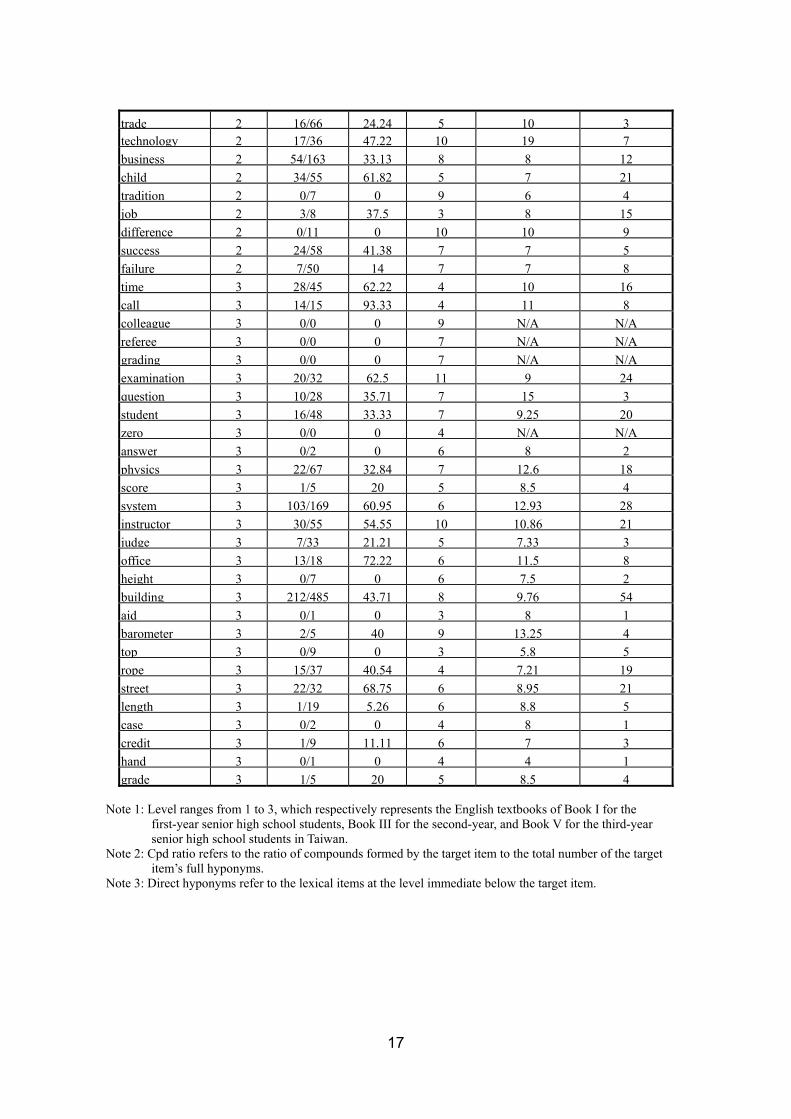
Appendix 2 Nouns Extracted from the Three Pieces of 200-word-text Target Item Direct Hyponyms
Item Level Cpd
Hyponym
Cpd Ratio
()
Length Avg Length Number
scientist 1 37174 21 9 13 20 tongue 1 04 0 6 0 0 taste 1 434 117 5 6 9 vinegar 1 35 60 7 11 3 soap 1 1415 93 4 9 8 food 1 12342310 53 4 8 15 nose 1 422 18 4 6 8 time 1 10 0 4 0 0 cold 1 23 666 4 8 1 test 1 811 727 4 9 5 person 1 315213235 238 6 8 401 potato 1 1016 625 6 11 5 mouth 1 310 30 5 4 6 apple 1 1730 566 5 10 3 smell 1 223 86 5 6 4 orange 1 89 888 6 11 3 slice 1 210 20 5 6 2 culture 2 2327 8519 7 19 7 language 2 4251210 3512 8 12 16 world 2 29 2222 5 11 3 end 2 2354 4259 3 6 14 heart 2 25 40 5 15 2 factor 2 1422 6364 6 12 6
16
trade 2 1666 2424 5 10 3 technology 2 1736 4722 10 19 7 business 2 54163 3313 8 8 12 child 2 3455 6182 5 7 21 tradition 2 07 0 9 6 4 job 2 38 375 3 8 15 difference 2 011 0 10 10 9 success 2 2458 4138 7 7 5 failure 2 750 14 7 7 8 time 3 2845 6222 4 10 16 call 3 1415 9333 4 11 8 colleague 3 00 0 9 NA NA referee 3 00 0 7 NA NA grading 3 00 0 7 NA NA examination 3 2032 625 11 9 24 question 3 1028 3571 7 15 3 student 3 1648 3333 7 925 20 zero 3 00 0 4 NA NA answer 3 02 0 6 8 2 physics 3 2267 3284 7 126 18 score 3 15 20 5 85 4 system 3 103169 6095 6 1293 28 instructor 3 3055 5455 10 1086 21 judge 3 733 2121 5 733 3 office 3 1318 7222 6 115 8 height 3 07 0 6 75 2 building 3 212485 4371 8 976 54 aid 3 01 0 3 8 1 barometer 3 25 40 9 1325 4 top 3 09 0 3 58 5 rope 3 1537 4054 4 721 19 street 3 2232 6875 6 895 21 length 3 119 526 6 88 5 case 3 02 0 4 8 1 credit 3 19 1111 6 7 3 hand 3 01 0 4 4 1 grade 3 15 20 5 85 4
Note 1 Level ranges from 1 to 3 which respectively represents the English textbooks of Book I for the
first-year senior high school students Book III for the second-year and Book V for the third-year senior high school students in Taiwan
Note 2 Cpd ratio refers to the ratio of compounds formed by the target item to the total number of the target itemrsquos full hyponyms
Note 3 Direct hyponyms refer to the lexical items at the level immediate below the target item
17
A Semantic Composition Method for Deriving Sense Representations of Determinative-Measure Compounds in E-HowNet
Chia-hung Tai Shu-Ling Huang Keh-Jiann Chen Institute of Information Science Academia Sinica
glaxy josieh kchen iissinicaedutw
㐀天ġ
㛔䭯婾㔯uArr䓐⭂慷墯⎰娆䁢ἳ炻䣢䭬⤪ỽuArr䓐佑䞍䵚䘬婆シ⎰ㆸ㨇Ἦ墯⎰娆䘬
婆シ堐忼ˤ椾ㆹᾹ⭂佑Ḯ㚱Ữ㚱旸㔠慷䘬⭂娆嶇慷娆䘬佑䞍䵚堐忼炻
叿ㆹᾹuArr䓐婆シ⎰ㆸ䘬夷憅ảỽ㕘䘬⭂慷娆䓊䓇῁怠䘬婆シ堐忼ʕ 䃞ㆹᾹ
婧㔜婆㕁普⎰姕妰婆シ妋㬏夷炻uArr䓐䘤婆シ妋㬏夷嶇侫ᶲᶳ㔯䘬娆Ἦ妋
㰢⭂慷娆䘬佑䞍䵚堐忼䘬㬏䔘炻槿栗䣢婆シ嶇妋㬏㚱 ĹĹĦ䘬㬋䡢䌯 ġʕ
Abstract
In this paper we take Determinative-Measure Compounds as an example to demonstrate how the E-HowNet semantic composition mechanism works in deriving the sense representations for all determinative-measure (DM) compounds which is an open set We define the sense of a closed set of each individual determinative and measure word in E-HowNet representation exhaustively We then make semantic composition rules to produce candidate sense representations for any newly coined DM Then we review development set to design sense disambiguation rules We use these heuristic disambiguation rules to determine the correct context-dependent sense of a DM and its E-HowNet representation The experiment shows that the current model reaches 88 accuracy in DM identification and sense derivation
斄挝娆烉婆シ⎰ㆸ炻⭂慷墯⎰娆炻婆シ堐忼炻佑䞍䵚炻䞍䵚
Keywords Semantic Composition Determinative-Measure Compounds Sense
Representations Extended How Net How Net
1 Introduction
Building knowledge base is a time consuming work The CKIP Chinese Lexical Knowledge Base has about 80 thousand lexical entries and their senses are defined in terms of the E-HowNet format E-HowNet is a lexical knowledge and common sense knowledge representation system It was extended from HowNet [1] to encode concepts Based on the
18
framework of E-HowNet we intend to establish an automatic semantic composition mechanism to derive sense of compounds and phrases from lexical senses [2][3] Determinative-Measure compounds (abbreviated as DM) are most common compounds in Chinese Because a determinative and a measure normally coin a compound with unlimited versatility the CKIP group does not define the E-HowNet representations for all DM compounds Although the demonstrative numerals and measures may be listed exhaustively their combination is inexhaustible However their constructions are regular [4] Therefore an automatic identification schema in regular expression [4] and a semantic composition method under the framework of E-HowNet for DM compounds were developed In this paper we take DMs as an example to demonstrate how the E-HowNet semantic
composition mechanism works in deriving the sense representations for all DM compounds
The remainder of this paper is organized as follows The section 2 presents the background
knowledge of DM compounds and sense representation in E-HowNet Wersquoll describe our
method in the section 3 and discuss the experiment result in the section 4 before we make
conclusion in the section 5
2 Background
There are numerous studies on determinatives as well as measures especially on the types of measures1 Tai [5] asserts that in the literature on general grammar as well as Chinese grammar classifiers and measures words are often treated together under one single framework of analysis Chao [6] treats classifiers as one kind of measures In his definition a measure is a bound morpheme which forms a DM compound with the determinatives enumerated below He also divides determinatives word into four subclasses
i Demonstrative determinatives eg 忁rdquo thisrdquo thatrdquo恋rdquohellip ii Specifying determinatives eg 㭷rdquoeveryrdquo ⎬rdquo eachrdquohellip
iii Numeral determinatives eg Ḵrdquotwordquo 䘦↮ᶱrdquothree percentagerdquo 䘦Ḽ⋩rdquo four hundred and fiftyrdquohellip
iv Quantitative determinatives eg ᶨrdquo onerdquo 㺧rdquo fullrdquo 姙rdquo manyrdquohellip Measures are divided into nine classes by Chao [6] Classifiers are defined as lsquoindividual measuresrsquo which is one of the nine kinds of measures
i classifiers eg 㛔rdquoa (book)rdquo 1 Chao [6] and Li and Thompson [7] detect measures and classifiers He [8] traces the diachronic names of
measures and mentions related literature on measures The dictionary of measures pressed by Mandarin Daily
News Association and CKIP [9] lists all the possible measures in Mandarin Chinese
19
ii classifier associated with V-O constructions eg ㇳ ldquohandrdquo iii group measures eg rdquopairrdquo iv partitive measures eg ṃrdquosomerdquo v container measures eg 䙺ldquoboxrdquo
vi temporary measures eg 幓rdquobodyrdquo vii Standard measures eg rdquometerrdquo
viii quasi-measure eg rdquocountryrdquo ix Measures with verb eg 㫉rdquonumber of timesrdquo
As we mentioned in the section of introduction Chao considers that determinatives are listable and measures are largely listable so D and M can be defined by enumeration and that DM compounds have unlimited versatility However Li and Thompson [7] blend classifiers with measures They conclude not only does a measure word generally not take a classifier but any measure word can be a classifier In Tairsquos opinion [5] in order to better understand the nature of categorization in a classifier system it is not only desirable but also necessary to differentiate classifiers from measure words These studies on the distinction between classifiers and measures are not very clear-cut In this paper we adopt the CKIP DM rule patterns and Part-of-Speeches for morpho-syntactic analysis and therefore inherit the definition of determinative-measure compounds (DMs) in [10] Mo et al define a DM as the composition of one or more determinatives together with an optional measure It is used to determine the reference or the quantity of the noun phrase that co-occurs with it We use the definition of Mo et al to apply to NLP and somewhat different from traditional linguistics definitions 21 Regular Expression Approach for Identifying DMs
Due to the infinite of the number of possible DMs Mo et al [10] and Li et al [4] propose to
identify DMs by regular expression before parsing as part of their morphological module in
NLP For example when the DM compound is the composition of one determinative eg
for numerals in (1) roughly rules (2a) (2b) or (2c) will be first applied and then rules (2d)
(2e) or (2f) will be applied to compose complex numeral structures and finally rules (2g) will
generate the pos Neu of numeral structures From the processes of regular expression the
numerals 534 and 319 in (1) is identified and tagged as Neu2
(1) 溻⊝534Ṣ⬴ㆸ319悱㕭
guli wubaisanshisi ren wancheng sanbaiyishijiu xiang zhi lu
encourage 534 persons to accomplish the travel around 319 villages
2 The symbol ldquoNeurdquo stands for Numeral Determinatives Generation rules for numerals are partially listed in(2)
20
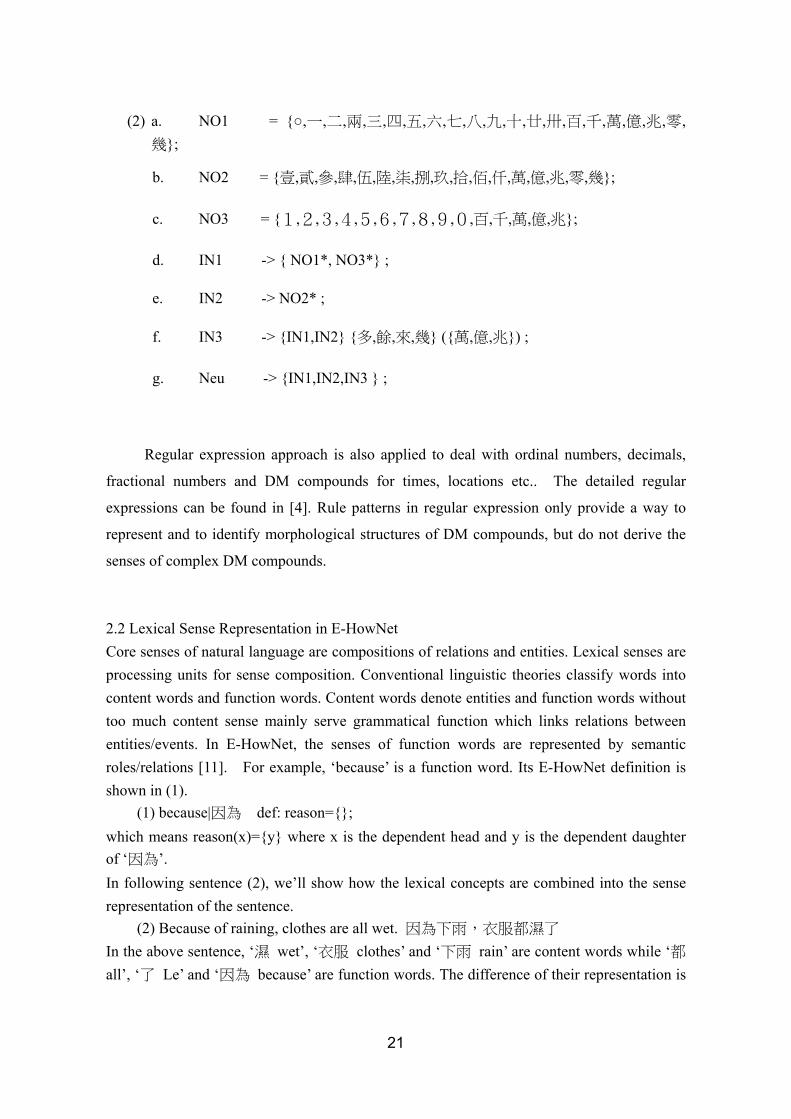
(2) a NO1 = ᶨḴimageᶱḼℕᶫℓḅ⋩⋭䘦⋫叔euro暞⸦
b NO2 = 屛倮ẵ映㝺䌾Ἐẇ叔euro暞⸦
c NO3 = 烀烁烂烃烄烅烆烇烈炿䘦⋫叔euro
d IN1 -gt NO1 NO3
e IN2 -gt NO2
f IN3 -gt IN1IN2 检Ἦ⸦ (叔euro)
g Neu -gt IN1IN2IN3
Regular expression approach is also applied to deal with ordinal numbers decimals
fractional numbers and DM compounds for times locations etc The detailed regular
expressions can be found in [4] Rule patterns in regular expression only provide a way to
represent and to identify morphological structures of DM compounds but do not derive the
senses of complex DM compounds
22 Lexical Sense Representation in E-HowNet Core senses of natural language are compositions of relations and entities Lexical senses are processing units for sense composition Conventional linguistic theories classify words into content words and function words Content words denote entities and function words without too much content sense mainly serve grammatical function which links relations between entitiesevents In E-HowNet the senses of function words are represented by semantic rolesrelations [11] For example lsquobecausersquo is a function word Its E-HowNet definition is shown in (1) (1) because|䁢 def reason= which means reason(x)=y where x is the dependent head and y is the dependent daughter of lsquo䁢rsquo In following sentence (2) wersquoll show how the lexical concepts are combined into the sense representation of the sentence (2) Because of raining clothes are all wet 䁢ᶳ暐炻堋㚵悥㽽Ḯ In the above sentence lsquo㽽 wetrsquo lsquo堋㚵 clothesrsquo and lsquoᶳ暐 rainrsquo are content words while lsquo悥 allrsquo lsquo瀈 Lersquo and lsquo䁢 becausersquo are function words The difference of their representation is
21
that function words start with a relation but content words have under-specified relations If a content word plays a dependent daughter of a head concept the relation between the head concept and this content word will be established after parsing process Suppose that the following dependent structure and semantic relations are derived after parsing the sentence (2) (3) S(reasonVP(HeadCb䁢|dummyVAᶳ暐)|themeNP(HeadNa堋㚵) | quantity Da悥 | HeadVh㽽|particleTa瀈)ˤ After feature-unification process the following semantic composition result (4) is derived The sense representations of dependent daughters became the feature attributes of the sentential head lsquowet|㽽rsquo (4) defwet|㽽
theme=clothing|堋䈑 aspect=Vachieve|忼ㆸ manner=complete|㔜 reason=rain|ᶳ暐
In (3) function word lsquo䁢 becausersquo links the relation of lsquoreasonrsquo between head concept lsquo㽽 wetrsquo and lsquoᶳ暐 rainrsquo The result of composition is expressed as reason(wet|㽽)=rain|ᶳ暐 since for simplicity the dependent head of a relation is normally omitted Therefore reason(wet|㽽)=rain|ᶳ暐 is expressed as reason=rain|ᶳ暐 theme(wet|㽽)=clothing|堋䈑 is expressed as theme=clothing|堋䈑 and so on 23 The sense representation for determinatives and measures in E-HowNet The sense of a DM compound is determined by its morphemes and the set of component morphemes are determinatives and measures which are exhaustively listable Therefore in order to apply semantic composition mechanism to derive the senses of DM compounds we need to establish the sense representations for all morphemes of determinatives and measures first Determinatives and measure words are both modifiers of nounsverbs and their semantic relation with head nounsverbs are well established We thus defined them by a semantic relation and its value like (5) and (6) bellowed (5) The definition of determinatives in E-HowNet
this 忁 def quantifier=definite|⭂ first椾 def ordinal=1 oneᶨ def quantity=1
We find some measure words contain content sense which need to be expressed but for some measure words such as classifiers their content senses are not important and could be neglect So we divided measure words into two types with or without content sense their
22
sense representations are exemplified below (6) The definition of measure words in E-HowNet a) Measure words with content sense
bowl䠿 def container=bowl|䠿 meter䰛 def length=meter| month㚰 def time=month|㚰
b) Measure words without content sense
㛔 copy defnull 攻 room defnull 㧋 kind defnull
3 Semantic Composition for DM Compounds
To derive sense representations for all DM compounds we study how to combine the E-HowNet representations of determinative and measure words into a DM compound representation and make rules for automatic composition accordingly Basically a DM compound is a composition of some optional determinatives and an optional measure It is used as a modifier to describe the quantity frequency container lengthhellipetc of an entity The major semantic roles played by determinatives and measures are listed in the Table 1
The basic feature unification processes [12]
If a morpheme B is a dependency daughter of morpheme A ie B is a modifier or an argument of A then unify the semantic representation of A and B by the following steps
Step 1 Identify semantic relation between A and B to derive relation(A)=B Note the possible semantic relations are shown in Table 1
Step 2 Unify the semantic representation of A and B by insert relation(A)=B as a sub-feature of A
It seems that a feature unification process can derive the sense representation of a DM compound as exemplified in (7) and (8) once its morpheme sense representations and semantic head are known (7) oneᶨ defquantity=1 + bowl䠿 def container=bowl|䠿
one bowlᶨ䠿 def container=bowl|䠿quantity=1 (8) this忁 def quantifier=definite|⭂ + 㛔 copy defnull
this copy忁㛔 def quantifier=definite|⭂
Table 1 Major semantic roles played by determinants and measures
Semantic Role DM
23
quantifier eg 忁ˣ恋ˣ㬌ˣ娚ˣ㛔ˣ屜ˣ㔅ˣˣ㝸ˣ媠
ordinal eg 䫔ˣ椾
qualification eg ᶲˣᶳˣ⇵ˣˣ柕ˣ㛓ˣ㫉ˣ椾ˣṾˣ检ˣ
ˣ㕩ˣṾˣˣˣ⎬
quantity eg ᶨˣḴˣ叔ˣ暁ˣ㭷ˣảỽˣᶨˣℐˣ㺧ˣ㔜ˣᶨ
ˣ劍⸚ˣ㚱䘬ˣᶨṃˣ悐ấˣ㚱ṃˣ姙ˣˣ⤥
ˣ⤥⸦ˣ⤥ṃˣ姙ˣˣ姙姙ˣ⸦姙ˣ㔠ˣ
㔠ˣ㔠ˣ㲘⋲ˣᶵˣᾳˣ⋲㔠ˣ媠
Formal=Ques eg ỽˣˣṨ湤
Quantity=over
approximate exact
eg 检ˣ姙ˣ嵛ˣˣ柕ˣ⤥⸦ˣ攳ˣ㔜ˣ㬋
position eg 㟴⫸ˣ昊⫸ˣˣ⫸ˣ㰈ˣ僼ˣ⫸
container eg 䙺(⫸)x ⋋(⫸)x 䭙(⫸)x 㩫⫸x 㪍(⫸)x 䯫(⫸)x 䮵(⫸)x
䆸⫸ˣ⊭()x 堳()x 㰈⫸ˣ䒞(⫸)x 㠞(⫸)x 倥ˣ仸(⫸)ˣ
䙮(⫸)ˣ拳(⫸)ˣ䰈(⫸)ˣ䚌(⫸)ˣ䠿ˣ㜗(⫸)ˣ⊢(⫸)ˣ
⋁(㸗⋁)x 䫺(⫸)x 㑼(⫸)x 䰖䫸ˣ㛻(⫸)x 勞⋁ˣˣ䙭ˣ
䫸ˣ䒊ˣ挔ˣ仠
length eg ˣ↮ˣˣˣᶰˣˣ慴ˣⶪ
ˣ䆇忈 ˣˣ⎳(inch)ˣ(feet)ˣ䡤(yard)ˣ⒑
(mile)ˣ (㴟)㴔ˣˣˣˣ慴ˣ慸ˣˣᶰˣ䰛ˣ
ˣ䰛ˣ㴟 ⒑ˣ劙ˣ劙慴ˣ劙ˣ劙ˣ䰛䨩ˣ
䰛ˣ䰛ˣ㮓䰛ˣ 劙⎳ˣ劙⒑ˣ⸜
size eg 䔅ˣ枫ˣⶪ䔅ˣ䆇忈䔅ˣˣ䔅ˣ↮ˣ䓚ˣ枫ˣ
㕡慴ˣ㕡ˣ㕡↮ˣ㕡ˣ㕡劙⒑ˣ
劙䔅
weight eg ˣ㕌ˣˣⶪ㕌ˣimageˣ㕌(㖍㕌)ˣ䙶⎠
(㕗)ˣ䡭ˣ㑼ˣ堉ˣimageˣˣ㕌ˣimageˣ拊ˣˣ
ˣ劙䡭ˣ劙imageˣ拊ˣ㮓ˣ㮓↮ˣẇˣ㮓
volume eg 㑖ˣ⋯(ⶪ⋯)ˣ䆇忈⋯ˣ⋯(㖍⋯)ˣ䙶⎠ˣ⑩
僓(pint)ˣasympἾ(gallon)ˣ呚俛(bushel)ˣ㔿ˣ䞛ˣ
䥱ˣ⎰ˣ⊢ˣ㔿ˣ㮓⋯ˣˣ䈡ˣ䇦ˣ䩳㕡䰛ˣ
䩳㕡䰛ˣ䩳㕡↮ˣ䩳㕡ˣ䩳㕡ˣ䩳↮慴ˣ
䩳㕡劙ˣ䞛ˣ㕃ˣ大大
time eg 䥺ˣ慸䥺ˣ䥺ˣ䥺揀ˣ↮ˣ↮揀ˣˣ揀ˣ溆ˣ
溆揀ˣ㗪ˣ㗪ˣ㚜ˣˣ㖔ˣ䲨(廒 12⸜) ˣᶾ䲨ˣ
(㖍)x 㗇㛇(䥖㊄ˣ忙ˣ) ˣ㚰ˣ㚰ấˣˣ⸜(庱ˣ㬚) ˣ
忙⸜ˣ㬚ˣ⸜ấˣ㘂ˣˣᶾˣ廑ˣ廑⫸ˣẋˣ㛇ˣ
⸜ˣ⸜ẋ
24
address eg ˣ䚩ˣⶆˣˣ悱ˣ㛹ˣ捖ˣ惘ˣ慴ˣ悉ˣ⋨ˣ
䪁ˣˣˣ㭝ˣ嘇ˣ㦻ˣ埾ˣⶪˣ㳚ˣˣ埿
place eg 悐ˣ⎠ˣ婚ˣ昊ˣ䥹ˣ䲣ˣ䳂ˣ偉ˣ⭌ˣ
duration eg昋(⫸)ˣ㚫ˣ㚫ˣᶳ⫸
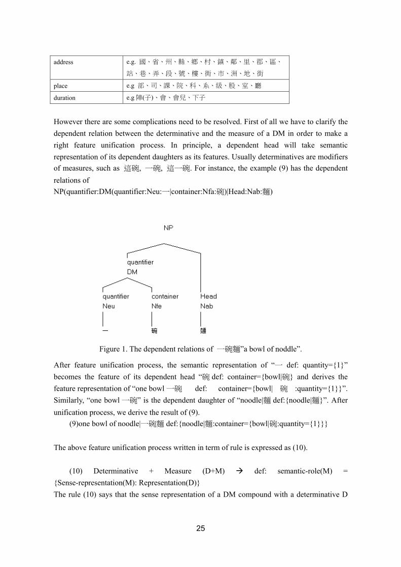
However there are some complications need to be resolved First of all we have to clarify the dependent relation between the determinative and the measure of a DM in order to make a right feature unification process In principle a dependent head will take semantic representation of its dependent daughters as its features Usually determinatives are modifiers of measures such as 忁䠿 ᶨ䠿 忁ᶨ䠿 For instance the example (9) has the dependent relations of NP(quantifierDM(quantifierNeuᶨ|containerNfa䠿)|HeadNab湝)
Figure 1 The dependent relations of ᶨ䠿湝rdquoa bowl of noddlerdquo
After feature unification process the semantic representation of ldquoᶨ def quantity=1rdquo becomes the feature of its dependent head ldquo䠿 def container=bowl|䠿 and derives the feature representation of ldquoone bowlᶨ䠿 def container=bowl| 䠿 quantity=1rdquo Similarly ldquoone bowlᶨ䠿rdquo is the dependent daughter of ldquonoodle|湝 defnoodle|湝rdquo After unification process we derive the result of (9) (9)one bowl of noodle|ᶨ䠿湝 defnoodle|湝container=bowl|䠿quantity=1 The above feature unification process written in term of rule is expressed as (10) (10) Determinative + Measure (D+M) def semantic-role(M) = Sense-representation(M) Representation(D) The rule (10) says that the sense representation of a DM compound with a determinative D
25
and a measure M is a unification of the feature representation of D as a feature of the sense representation of M as exemplified in (9) However a DM compound with a null sense measure word such as lsquothis copy|忁㛔rsquo lsquo a copy|ᶨ㛔rsquo or without measure word such as lsquothis three|忁ᶱrsquo will be exceptions since the measure word cannot be the semantic head of DM compound The dependent head of determinatives become the head noun of the NP containing the DM and the sense representation of a DM is a coordinate conjunction of the feature representations of its morphemes of determinatives only For instance in (8) lsquocopyrsquo has weak content sense we thus regard it as a null-sense measure word and only retain the feature representation of the determinative as the definition of ldquothis copy|忁㛔rdquo The unification rule for DM with null-sense measure is expressed as (11) (11) Determinative + Null-sense Measure (D+M) def Representation(D) If a DM has more than one determinative we can consider the consecutive determinatives as one D and the feature representation of D is a coordinate conjunction of the features of all its determinatives For instance ldquothis one|忁ᶨrdquo and ldquothis one|忁ᶨ㛔rdquo both are expressed as ldquoquantifier=definite|⭂ quantity=1rdquo Omissions of numeral determinative are occurred very often while the numeral quantity is ldquo1rdquo For instance ldquo忁㛔rdquo in fact means ldquothis one|忁ᶨ㛔rdquo Therefore the definition of (8) should be modified as 忁㛔 def quantifier=definite|⭂ quantity=1 The following derivation rules cover the cases of omissions of numeral determinative (12) If both numeral and quantitative determinatives do not occur in a DM then the feature quantity=1 is the default value of the DM Another major complication is that senses of morphemes are ambiguous The feature unification process may produce many sense representations for a DM compound Therefore sense disambiguation is needed and the detail discussions will be in the section 31 Members of every type of determinatives and measures are exhaustively listable except numeral determinatives Also the formats of numerals are various For example ldquo5020rdquo is equal to ldquoḼ暞Ḵ暞rdquo and ldquoḼ⋫暞Ḵ⋩rdquo and ldquoḼ⋫Ḵ⋩rdquo So we have to unify the numeral representation into a standard form All numerals are composition of basic numeral as shown in the regular expressions (2) However their senses are not possible to define one by one We take a simple approach For all numeral their E-HowNet sense representations are expressed
26
as themselves For example 5020 is expresses as quantity=5020 and will not further define what is the sense of 5020 Furthermore all non-Arabic forms will be convert into Arabic expression eg ldquoḼ⋫暞Ḵ⋩rdquo is defined as quantity=5020 The other problem is that the morphological structures of some DMs are not regular patterns Take ldquoimageᾳ⋲ two and halfrdquo as an example ldquo⋲ halfrdquo is not a measure word So we collect those word like ldquomany ⋲half ⸦many ᶲup big Ἦmorerdquo for modify the quantity definition So we first remove the word ldquo⋲rdquo and define the ldquoimageᾳrdquo as quantity=2 Because the word ldquo⋲rdquo means quantity=05 we define the E-HowNet definition for ldquoimageᾳ⋲rdquo as quantity=25 For other modifiers such as ldquo many ⸦ many 检 more Ἦ morerdquo we use a function over() to represent the sense of ldquomorerdquo such as ldquo⋩ᾳ more than 10rdquo is represented as quantity=over(10) The appendix A shows the determinatives and measures used and their E-HowNet definition in our method Now we have the basic principles for compositing semantics of DM under the framework of E-HowNet Below steps is how we process DMs and derive their E-HowNet definitions from an input sentence
I Input a Chinese sentence II Apply regular expression rules for DM to identify all possible DM candidates in the
input sentence III Segment DM into a sequence of determinatives and measure words IV Normalize numerals into Arabic form if necessary V Apply feature unification rules (10-12) to derive candidates of E-HowNet
representations for every DM VI Disambiguate candidates for each DM if necessary VII Output DM Compounds in E-HowNet representation
For an input Chinese sentence we use the regular expression rules created by Li et al [2006] to identify all possible DMs in the input sentence Then for every DM compound we segment it into a sequence of determinatives and measures If any numeral exists in the DM every numeral is converted into decimal number in Arabic form For every DM we follow the feature unification principles to composite semantics of DM in E-HowNet representations and produce possible ambiguous candidates The final step of sense disambiguation is described in the following section 31 Sense Disambiguation Multiple senses will be derived for a DM compound due to ambiguous senses of its morpheme components For instance the measure word rdquo柕 headrdquo has either the sense of
27
柕|head such as ldquo㺧柕䘥檖 full head of white hairsrdquo or the null sense in rdquoᶨ柕䈃 a cowrdquo Some DMs are inherent sense ambiguous and some are pseudo ambiguous For instances the above example ldquoᶨ柕rdquo is inherent ambiguous since it could mean ldquofull headrdquo as in the example of ldquoᶨ柕䘥檖 full head of white hairsrdquo or could mean ldquoone + classifierrdquo as in the example of rdquoᶨ柕䈃 a cowrdquo For inherent ambiguous DMs the sense derivation step will produce ambiguous sense representations and leave the final sense disambiguation until seeing collocation context in particular seeing dependent heads Some ambiguous representations are improbable sense combination The improbable sense combinations should be eliminated during or after feature unification of D and M For instance although the determiner ldquoᶨrdquo has ambiguous senses of ldquoonerdquo ldquofirstrdquo and ldquowholerdquo but ldquoᶨrdquo has only one sense of ldquoone meterrdquo so the other sense combinations should be eliminated The way we tackle the problem is that first we find all the ambiguous Ds and Ms by looking their definitions shown in the appendix A We then manually design content and context dependent rules to eliminate the improbable combinations for each ambiguous D or M types For instance according to the appendix A ldquo柕rdquo has 3 different E-HowNet representations while functions as determinant or measure ie ldquodefnullrdquo ldquodefhead|柕 rdquo and ldquodefordinal=1rdquo We write 3 content or context dependent rules below to disambiguate its senses
(13) 柕rdquoheadrdquo Nfa E-howNet ldquodefnullrdquo while E-HowNet of head word is ldquo≽䈑(animate|䓇䈑rdquo and itrsquos subclass
(14) 柕ldquoheadldquo Nff E-howNet ldquodef柕rdquo while pre-determinant isᶨ(Neqa)rdquoonerdquo or 㺧rdquofullrdquo orℐrdquoallrdquo or 㔜rdquototalrdquo
(15) 柕rdquofirstrdquo Nes E-howNet ldquodefordinal=1rdquo while this word is being a demonstrative determinatives which is a leading morpheme of the compound
The disambiguation rules are shown in appendix B In each rule the first part is the word and its part-of-speech Then the E-HowNet definition of this sense is shown and followed by the condition constraints for this sense If there is still ambiguities remained after using the disambiguation rule we choice the most frequent sense as the result
4 Experiment and Discussion
We want to know how good is our candidate production and how good is our disambiguation rule We randomly select 40628 sentences (7536 DM words) from Sinica Treebank as our development set and 16070 sentences (3753 DM words) as our testing set We use development set for designing disambiguation rules and semantic composition rules Finally we derive 36 contextual dependent rules as our disambiguation rules We randomly select 1000 DM words from testing set We evaluate the composition quality of DMs with E-HowNet representation before disambiguation For 1000 DM words the semantic
28
composition rules produce 1226 candidates of E-HowNet representation from 939 words The program fails to produce E-HowNet representations for the rest of 61 words because of undefined morphemes There are 162 words out of the 939 words having ambiguous senses The result shows that the quality of candidates is pretty good Table 2 gives some examples of the result For testing the correctness of our candidates we manually check the format of 1226 candidates Only 5 candidates out of 1226 are wrong or meaningless representations After disambiguation processes the resulting 1000 DM words in E-HowNet representation are judged manually There are 880 correct E-HowNet representations for 1000 DM words in both sense and format It is an acceptable result Among 120 wrong answers 57 errors are due to undefined morpheme 28 errors are unique sense but wrong answer and the number of sense disambiguation errors is 36 Therefore accuracy of sense disambiguation is (162-36)162=0778
Table 2 The result of semantic composition for DM compounds
DM Compounds E-HowNet Representation Ḵ⋩叔 defrole=money|屐quantity=200000 ᶨᾳ defqualification=other|quantity=1 Ḵ䘦ᶱ⋩ℕ↮ defrole=↮㔠quantity=236 ⇵Ḽ deftime=day| 㖍 qualification=preceding| ᶲ 㫉
quantity=5 ᶨ䘦ᶨ⋩ℕ溆ᶫ
euro伶 defrole=伶quantity=11670000000
After data analysis we conclude the following three kinds of error types
A Unknown domain error ᶫ㡺rdquo7th batterrdquo ᶫrdquo7th inningrdquo Because there is no text related to baseball domain in development set we get poor performance in dealing with the text about baseball The way to resolve this problem is to increase the coverage of disambiguation rules for the baseball domain
B Undefined senses and morphemes 㭷ᶱᾳldquoeach threerdquo We do not define the sense of 㭷 rdquoeachrdquo and we only define㭷 rdquoallrdquo so we have to add the sense of ldquoeachrdquo in E-HowNet representation about㭷 㚱ᶱỵ rdquothere are three personsrdquo ᶨᾳ rdquothe samerdquo Because 㚱 ldquohaverdquo and rdquothe samerdquo do not appear in our determinative list it is not possible to composite their E-HowNet definitions
C Sense ambiguities In parsed sentence NP(propertyDMᶲ⋲⟜rdquofirst half rdquo|HeadDMḴ⋩↮rdquotwenty
29
minutes or twenty pointsrdquo) The E-HowNet representation ofḴ⋩↮rdquotwenty minutes or twenty pointsrdquo can be defined as ldquodefrole=↮㔠quantity=20rdquo or ldquodeftime=↮揀quantity=20rdquo More context information is needed to resolve this kind of sense ambiguity
For unknown domain error and undefined rule the solution is to expand the disambiguation rule set and sense definitions for morphemes For sense ambiguities we need more information to disambiguate the true sense
5 Conclusion
E-HowNet is a lexical sense representational framework and intends to achieve sense representation for all compounds phrases and sentences through automatic semantic composition processing In this paper we take DMs as an example to demonstrate how the semantic composition mechanism works in E-HowNet to derive the sense representations for all DM compounds We analyze morphological structures of DMs and derive their morphological rules in terms of regular expression Then we define the sense of all determinatives and measure words in E-HowNet definition exhaustively We make some simple composition rules to produce candidate sense representations for DMs Then we review development set to write some disambiguation rules We use these heuristic rules to find the final E-HowNet representation and reach 88 accuracy The major target of E-HowNet is to achieve semantic composition For this purpose we defined word senses of CKIP lexicon in E-HowNet representation Then we try to automate semantic composition for phrases and sentences However there are many unknown or compound words without sense definitions in the target sentences DM compounds are occurring most frequently and without sense definitions Therefore our first step is to derive the senses of DM words In the future we will use similar methods to handle general compounds and to improve sense disambiguation and semantic relation identification processing We intend to achieve semantic compositions for phrases and sentences in the future and we had shown the potential in this paper
Acknowledgement
This research was supported in part by the National Science Council under a Center Excellence Grant NSC 96-2752-E-001-001-PAE and Grant NSC96-2221-E-001-009
References
[1] Zhendong Don amp Qiang Dong 2006 HowNet and the Computation of Meaning World Scientific Publishing Co Pte Ltd
[2] 昛ˣ湫㵹漉ˣ㕥枛ˣ昛zwj炻2005b炻橼⫿䞍䵚㝞㥳ᶳ≇傥娆堐忼炻䫔ℕ㻊婆娆婆シ䞼妶㚫炻攨
30
[3] Shu-Ling Huang You-Shan Chung Keh-Jiann Chen 2008 E-HowNet- an Expansion of HowNet The First National HowNet Workshop Beijing China
[4] Li Shih-Min Su-Chu Lin Chia-Hung Tai and Keh-Jiann Chen 2006 A Probe into Ambiguities of Determinative-Measure Compounds International Journal of Computational Linguistics amp Chinese Language Processing Vol 11 No 3 pp245-280
[5] Tai J H-Y Chinese classifier systems and human categorization In Honor of William S-Y Wang Interdisciplinary Studies on Language and Language Change ed by M Y Chen
and O J-L Tzeng Pyramid Press Taipei 1994 pp 479-494
[6] Chao Y-R A grammar of Spoken Chinese University of California Press Berkeley 1968
[7] Li C N and S A Thompson Mandarin Chinese A Functional Reference Grammar
University of California Press Berkeley 1981
[8] ỽ㜘(He J) 䎦ẋ㻊婆濌娆䞼䨞 㮹㕷䇰䣦 澱Ṕⶪ 2002
[9] 湫ṩ 昛zwj 岜ㄞ晬(䶐叿) 婆㖍⟙濌娆 婆㖍⟙䇰䣦 澱 1997
[10] Mo R-P Y-J Yang K-J Chen and C-R Huang Determinative-Measure Compounds in Mandarin Chinese Their Formation Rules and Parser Implementation In Proceedings of ROCLING IV (ROC Computational Linguistics Conference) 1991 National Chiao-Tung University Hsinchu Taiwan pp 111-134
[11] Chen Keh-Jiann Shu-Ling Huang Yueh-Yin Shih Yi-Jun Chen 2005a Extended-HowNet- A Representational Framework for Concepts OntoLex 2005 - Ontologies and Lexical Resources IJCNLP-05 Workshop Jeju Island South Korea [12] Duchier D Gardent C and Niehren J (1999a) Concurrent constraint programming in Oz
for natural language processing Lecture notes httpwwwpsuni-sbde~niehren
oz-natural-language-scripthtml
Appendix A Determinative and measure word in E-HowNet representation
⭂娆(Determinative word)
⭂
31
D1-gt 忁ˣ恋ˣ㬌ˣ娚ˣ㛔ˣ屜ˣ㔅ˣˣ㝸ˣ媠 def quantifier=definite|⭂烊忁ṃˣ恋ṃ def quantifier=definite|⭂ quantity=some|ṃ
D2-gt 䫔ˣ椾 def ordinal=D4
D3-gt ᶲ ˣ ⇵ def qualification=preceding| ᶲ 㫉 ˣ ᶳ ˣ def qualification=next|ᶳ㫉ˣ柕ˣ椾 defordinal=1ˣ㛓 def qualification=last| 㚨ˣ㫉 defordinal=2
ᶵ⭂
D4-gt ᶨˣḴˣ叔ˣ暁 def quantity=1ˣ2ˣ10000ˣ2 or defordinal=1ˣ2ˣ10000ˣ2
D5-gt 䓚ˣḁ def ordinal=1ˣ2
D6-gt Ṿˣ检ˣˣ㕩ˣṾˣˣ def qualification=other|
D7-gt 㭷ˣảỽˣᶨˣℐˣ㺧ˣ㔜ˣᶨ def quantity=all|ℐ
D8-gt ⎬ def qualification=individual|↮䘬
D9-gt 劍⸚ˣ㚱䘬ˣᶨṃˣ悐ấˣ㚱ṃ def quantity=some|ṃ
D10-gt ⋲ def quantity=half|⋲
D11-gt ˣ⸦ def quantity=Ques
D12-gt ỽˣˣṨ湤 def fomal=Ques
D13-gt㔠ˣ姙ˣˣ⤥ˣ⤥⸦ˣ⤥ṃˣˣ姙姙ˣ㔠ˣ㔠ˣᶵˣ㲘⋲ˣ⋲㔠ˣ媠 def quantity=many|x 姙ˣ㔠ˣ⸦姙ˣᾳ def quantity=few|
D14-gt检ˣ姙ˣ def approximate()ˣ嵛ˣ㔜ˣ㬋 def exact()ˣ柕ˣ⤥⸦ˣ攳ˣ def over()
D15-gt0ˣ1ˣ2ˣ3ˣ4ˣ5ˣ6ˣ7ˣ8ˣ9 def quantity=1ˣ2ˣ3ˣ4
32
慷娆(Measure word)
㚱婆シ慷娆(Measures with content sense )
Nff-gt 㙓㗪慷娆mdash幓ˣ柕ˣ共ˣ滣⫸ˣˣ偂⫸ˣㇳˣ儛 def幓柕 hellip
Nff-gt 㙓㗪慷娆mdash㟴⫸ˣ昊⫸ˣˣ⫸ˣ㰈ˣ僼ˣ⫸ def position=㟴⫸昊⫸quantity=all|ℐ
Nfe-gt 慷娆mdash䙺(⫸)ˣ⋋(⫸)ˣ䭙(⫸)ˣ㩫⫸ˣ㪍(⫸)ˣ䯫(⫸)ˣ䮵(⫸)ˣ䆸 ⫸ˣ⊭()ˣ堳()ˣ㰈⫸ˣ䒞(⫸)ˣ㠞(⫸)ˣ倥ˣ仸(⫸)ˣ䙮(⫸)ˣ拳(⫸)ˣ 䰈(⫸)ˣ䚌(⫸)ˣ䠿ˣ㜗(⫸)ˣ⊢(⫸)ˣ⋁(㸗⋁)ˣ䫺(⫸)ˣ㑼(⫸)ˣ䰖䫸ˣ 㛻(⫸)ˣ勞⋁ˣˣ䙭ˣ䫸ˣ䒊ˣ挔ˣ仠 def container=䙺⋋
Nfg-gt 㧁㸾慷娆mdash
堐攟䘬炻⤪烉ˣ↮ˣˣˣᶰˣˣ慴ˣⶪˣ䆇
忈 ˣˣ⎳(inch)x (feet)x 䡤(yard)x ⒑(mile)x (㴟)㴔ˣˣˣˣ慴ˣ慸ˣˣᶰˣ䰛ˣˣ䰛ˣ㴟 ⒑ˣ劙ˣ劙慴ˣ劙ˣ劙ˣ䰛䨩ˣ䰛ˣ䰛ˣ㮓䰛ˣ 劙⎳ˣ劙⒑ˣ⸜ˤ def length=↮
堐朊䧵䘬炻⤪烉䔅ˣ枫ˣⶪ䔅ˣ䆇忈䔅ˣˣ䔅ˣ↮ˣ䓚ˣ枫ˣ㕡
慴ˣ㕡ˣ㕡↮ˣ㕡ˣ㕡劙⒑ˣ劙䔅 dʕef size=䔅
堐慵慷䘬炻⤪烉ˣ㕌ˣˣⶪ㕌ˣimageˣ㕌(㖍㕌)ˣ䙶⎠(㕗)ˣ䡭ˣ㑼ˣ堉ˣimageˣˣ㕌ˣimageˣ拊ˣˣˣ劙䡭ˣ劙imageˣ拊ˣ
㮓ˣ㮓↮ˣẇˣ㮓ˤdef weight=
堐慷䘬炻⤪烉㑖ˣ⋯(ⶪ⋯)x 䆇忈⋯ˣ⋯(㖍⋯)x 䙶⎠ˣ⑩僓(pint)ˣasympἾ(gallon)ˣ呚俛(bushel)ˣ㔿ˣ䞛ˣ䥱ˣ⎰ˣ⊢ˣ㔿ˣ㮓⋯ˣˣ䈡ˣ䇦ˣ䩳㕡䰛ˣ䩳㕡䰛ˣ䩳㕡↮ˣ䩳㕡ˣ䩳㕡
ˣ䩳↮慴ˣ䩳㕡劙ˣ䞛ˣ㕃ˣ大大ˤdef volume=㑖⋯
堐㗪攻䘬炻⤪烉䥺ˣ慸䥺ˣ䥺ˣ䥺揀ˣ↮ˣ↮揀ˣˣ揀ˣ溆ˣ溆揀ˣ
㗪ˣ㗪ˣ㚜ˣˣ㖔ˣ䲨(廒 12⸜) ˣᶾ䲨ˣ(㖍)ˣ㗇㛇(䥖㊄ˣ忙ˣ) ˣ㚰ˣ㚰ấˣˣ⸜(庱ˣ㬚) ˣ⸜ấˣ㘂ˣˣˤdeftemporal=䥺㚰hellip 忙⸜ˣ㬚 defduration=⸜
堐拊䘬炻⤪烉↮ˣ奺(㮃)ˣ()ˣ⟲ˣimageˣẌˣ䚏㭼ˣ㱽恶(㚿)ˣ彐ˣ楔ˣ挲ˣ䚏ⶫˣ伶ˣ伶慹ˣὧˣ慴ˣ㖍ˣˣ㷗ˣṢ
㮹ˤdef role=↮ hellipmoney|屐 hellip䚏ⶫhellip
Ṿ烉ˣㇻ(dozen)x Ẍˣ䵠(⋩㡅)x 嗧(gross)x 䰖(great gross)x 䃎俛ˣ⋫rceilˣẇrceilˣ䆕ˣ⋫䒎ˣẇ䒎ˣặ䈡ˣ楔≃ˣ䇦㟤(erg)ˣ䒎䈡ˣ䒎ˣrceil嶗慴ˣrceilˣẇ崓ˣỵˣ卓俛ˣ㮓ˣ⋫崓ˣ㫸⥮ˣ忼ˣ崓ˣ㱽䫔ˣ
䈃枻ˣ崓ˣ⬱ˣ㲊ˣ崓勚ˣ↮居ˣ㮓⬱ˣ慴ˣ慴ˣ㮓慴ˤ
def quantity=ㇻhellip䃎俛
33
Nfh-gt 㸾慷娆mdash
埴㓧㕡朊炻⤪烉悐x ⎠x 婚x 昊x 䥹x 䲣x 䳂x 偉x ⭌x ʕ def location=悐⎠
㗪攻㕡朊炻⤪烉ᶾˣ廑ˣ廑⫸ˣẋˣ㛇ˣ⸜ˣ⸜ẋ def time=㛇⸜ẋ 㚫ˣ㚫ˣ昋(⫸) ˣᶳ⫸ def duration=TimeShort|䞕㗪攻
㕡䘬炻⤪烉朊()ˣ㕡朊ˣ怲()ˣ㕡ˤdef direction=EndPosition|䪗ˣ柕() def direction=aspect|ldquo
枛㦪䘬炻⤪烉ˣ㜧ˣ䭨ˤdef quantity=㜧
柣䌯䘬炻⤪ˣ㫉ˣ念ˣ嵇ˣᶳˣ怕ˣ枧ˣˣˣ斄ˣ儛ˣˣˣ柕ˣˣ䛤ˣˣˣ㥴ˣ㥴⫸ˣ㜧ˣ䇰⫸ˣ杕ˣ杕⫸ˣ㡺ˣ㡵ˣ
㡵⫸ˣ憅ˣ㥵䞃ˣ㥵ˣ䟚ˣˣ廒ˣˣ嶌ˣ⎰ˣ䤐ˤDeffrequency=D4 D15 ↮ defrole= ↮ 㔠 quantity=D4D15 ˣ 㬍 def 㬍 ˣ 䭕defrole=䭕quantity=D4D15ˣ㚚 def㚚quantity=D4D15
Nfc-gt 佌 橼 慷 娆mdash ˣ 暁 defquantity=double| 墯 ˣ ( 䲣 ) ˣ defquantity=mass|䛦 manner= InSequence|㚱 ˣ defquantity=mass| 䛦 manner=relevant|䚠斄 ˣ defquantity=mass|䛦 dimension=linear|䶂 ˣ ˣˣ佌ˣề()ˣ䤐ˣ㈡ def quantity=mass|䛦ˣ䳬 def quantity=mass| 䛦 manner=relevant|䚠斄ˣ䩑 def quantity=mass|䛦cause=assemble|倂 普 ˣ䧖ˣ栆ˣ㧋 def kind(object|䈑橼) ˣ䮯 defquantity=mass| 䛦 cause=assemble| 倂普ˣ䔲 defquantity=mass|䛦cause=pile|㓦ˣ䳖 defquantity=mass|䛦cause=wrap|⊭䳖ˣ defquantity=mass| 䛦 cause=assemble|倂普 ˣ昲defquantity=mass|䛦manner= InSequence|㚱 ˣ defkind(object|䈑橼)
Nfd-gt悐↮慷娆mdashṃ defquantity=some|ṃˣ悐↮(ấ)ˣ㲉ˣ䵡ˣ㑖ˣ偉ˣ䀀ˣ 㰒ˣⷞˣˣ䭨 def quantity=fragment|悐ˣ def quantity=fragment| 悐shape=round|x def quantity= fragment|悐cause=pile|㓦x def quantity= fragment|悐cause=hold|ˣⰌˣ慵 def quantity= fragment| 悐shape=layered|䔲
䃉婆シ慷娆(null-sense Measures)
Nfa-gt ᾳ橼慷娆mdash㛔ˣˣ䒋ˣ悐ˣ㝬ˣˣ嗽ˣ㛇ˣ漋ˣ⟜ˣ㛝ˣ枪ˣ⟝ˣ忻ˣ枻ˣ拈ˣ㢇(⸊)ˣ㨼(㨼⫸)ˣˣˣ䘤ˣ↮(ấ)ˣ㚵ˣᾳ(䬯)ˣ㟡ˣ埴ˣˣẞˣˣ㝞ˣˣˣ敽ˣ䭨ˣˣˣˣ∹ˣ晣ˣˣ䚆ˣˣ㝅(㓗)ˣ㦩ˣˣˣ㟒ˣˣ䁟ˣ庠ˣˣ㢝ˣ㫦ˣ⭊ˣ廃ˣ䰺ˣ廒ˣ㝂ˣ朊ˣ攨ˣ
ˣ⋡ˣ䭯ˣ䇯ˣˣ刀ˣˣ椾ˣḀˣ多ˣ柕ˣ㡅ˣˣˣˣⶾˣ柮ˣ
ˣˣℲˣảˣˣˣỵˣ枩ˣ叱ˣˣˣ䎕ˣ⒉ˣ䥹ˣˣˣ枭ˣ
崟ˣ攻ˣ柴ˣ䚖ˣ㊃ˣ偉ˣˤdef null
34
Nfc-gt 佌橼慷娆mdash⬿ˣ䔒ˣ䔎ˣ梸ˣ埴ˣlowast(Ẁ)ˣ咔ˣ䫮ˣˣ䴹()ˣ偶ˣˣ悐ˣ㳦ˣ嶗ˣˣ句ˣ㜇ˣⷕˣ刚ˣ㓌ˣ枭ˤdef null
Nfd-gt 悐↮慷娆mdashˣ⟲ˣ㺜ˣ㪬ˣˣ㉙ˣ㭝ˣ䴚ˣ溆ˣ䇯ˣˣˣ⋡ˣ䔳ˣ昶ˣˣ㲊ˣ忻ˤdef null
Nfb-gt 徘屻⎰䓐䘬慷娆mdash忂ˣˣ枻ˣ䚌ˣˣ䔒ˤdef null
Nfi-gt ≽慷娆mdashˣ㫉ˣ念ˣ嵇ˣᶳˣ怕ˣ䔒ˣ倚ˣ枧ˣˣˣṿˣ奢ˣ枻ˣ斄ˣㇳ 炷x炸ˣ炷柕炸x ˣ䛤ˣˣ㥴(⫸)x 㜧(⫸)x 杕(⫸)x 㡺ˣ㡵炷⫸炸x 昋ˣ憅ˣ䭕ˣ㥵炷䞃炸x 㥵ˣ䟚ˣ⟜ˣˣ廒ˣ㚚ˣ嶌ˣ姀ˣ⎰ˣ䤐ˤdef null
Nfh-gt 㸾慷娆
㚠䯵㕡朊炻⤪烉䇰ˣℲˣ䶐ˣˣ䪈ˣ朊ˣ䭨ˣ普ˣˤdef null
䫮int㕡朊炻⤪烉䫮ˣint()ˣ㨓ˣ寶ˣ䚜ˣ㐯ˣˣ㊹ˣ⇼ˣ戌()ˣˣ溆ˣ㟤()ˤdef null
Ṿ烉
䦳ˣἄ(ἳᶨ⸜㚱imageἄ)ˣˣㆸˤdef null
(ἳ⸜uArrḼˣᶨ↮ᶨ悥ᶵ傥拗)ˤdef null
㮓(叔↮ᶨ)ˣ䴚(⋩叔↮ᶨ)(ἳᶨ䴚ᶨ㮓悥ᶵⶖ)ˤ
ˣˣ尉旸ˣˤdef null
攳(攳慹)ˣ倗(ἳᶲᶳ倗ᶵ䧙)ˤdef null
幵ˣⷓˣ㕭ˣˣ䆇ˣẵˣ䎕ˣˣ忋ˣ䎫ˣ㲊ˣ䪗ˤdef null
⎰ˣˣ㐢ˣ㳩ˣ䫱ˣ䤐ˣ㠧ˣ㡺ˣ倚ˣ㫉ˤdef null
Appendix B The rule for candidate disambiguation
head-based rule
egᶨ Neu defquantity=1 while part-of-speech of head word is Na except the measure word is 幓 rdquobodyrdquo or 共 rdquofacerdquo or 滣⫸ rdquonoserdquo or rdquomouthrdquo or 偂 ⫸rdquobellyrdquo or 僼rdquocavityrdquo
eg⟲Nfgdefrole=money|屐 while E-HowNet representation of head word is ldquomoney|屐rdquo or null or head word is 拊rdquomoneyrdquo or 伶慹rdquodollarrdquo or the s uffix of word isrdquocurrencyrdquo and previous word is not D1
⟲Nfddefnull otherwise use this definition
eg朊Nfadefnull while part-of-speech of head word is Nab
35
朊Nfhdefdirection=aspect|ldquo otherwise use this one
eg柕Nfadefnull while head word is Nab and E-HowNet representation of head word is ldquo≽䈑animate|䓇䈑rdquo and itrsquos subclass
柕Nfhdefdirection=EndPosition|䪗 if part-of-speech of head word is Na do not use this definition The previous word usually are 忁 rdquothisrdquo or 恋 rdquothatrdquo or rdquoanotherrdquo
egAll Nfi deffrequency= while part-of-speech of head word is Verb ie E-HowNet representation of head word is event|ḳẞ and itrsquos subclass Except POS V_2 and VG
All Nfidefnull while part-of-speech of head word is Noun ie E-HowNet of head word is object|䈑橼 and itrsquos subclass
eg悐 偉hellipNfhdeflocation= if part-of-speech of head word is Na or previous word is 忁rdquothisrdquo or恋rdquothatrdquo or㭷rdquoeveryrdquo do not use this definition
悐偉hellipNfadefnull otherwise use this definition
eg 䚌 Nfedefcontainer=plate| 䚌 while head word is food ie E-HowNet representation of head word is edible|梇䈑 and itrsquos subclass
䚌Nfbdefnullotherwise use this one
eg↮ Nfg defrole=↮ while head word is 拊 ldquomoneyrdquo ie E-HowNet representation of head word is money|屐 and itrsquos subclass
↮Nfg defsize= ↮ while head word is ldquolandrdquo ie E-HowNet representation of head word is land|映 and itrsquos subclass
↮Nfa defnull while part-of-speech of head word is Na or Nv For example ᶨ↮侽俀烊⋩↮≃㯋烊Ḽ↮䅇
eg溆NfhNfddefnull while part-of-speech of head word is Nab If part-of-speech of head word is V Naa or Nad do not use this definition
collocation-based rule
eg↮Nfhdefrole=score|↮㔠quantity=D4D15 while the sentence also contains the words侫 rdquogive an examrdquo (E-HowNet representation is exam|侫娎) or rdquogetrdquo (E-HowNet representation is obtain|) orrdquoloserdquo (E-HowNet representation is lose|) then use this definition
36
eg↮Nfgdeftime=minute|↮揀 if the sentence contains the word㗪rdquohourrdquo or揀 柕rdquohourrdquo
egimage Nfgdefweight=image if the sentence contains the word 慵rdquoweightrdquo or 慵 慷rdquoweightrdquo
imageNfgdefrole=money|屐 if the sentence contains the word 戨rdquosliverrdquo or 拊rdquomoneyrdquo or 湫慹rdquogoldrdquo
pre-determinant-based rule
eg柕 Nffdefhead|柕 while pre-determinant is ᶨ(Neqa)rdquoonerdquo or 㺧rdquofullrdquo or ℐrdquoallrdquo or 㔜rdquototalrdquo
eg儛 Nffdefleg|儛 while pre-determinant is ᶨ(Neqa)rdquoonerdquo or 㺧rdquofullrdquo or ℐ ldquoallrdquo or 㔜rdquototalrdquo and part-of-speech of head word is not Na
儛 Nfideffrequency= while part-of-speech combination is V+D4D15+儛
eg溆Nfg deftime=溆 while part-of-speech of pre-determinant is D4 or D15(1~24) and part-of-speech of previous word is not D1 or previous word is not 㚱rdquohaverdquo
eg廒Nfgdeftime=廒 while pre-determinant is 䫔 rdquo a function word placed in front of a cardinal number to form an ordinal numberrdquo or 椾rdquofirstrdquo
determinative-based rule
egᶨˣḴ1ˣ2image Neu defordinal= the determinant of word is䫔 㮹 大 ⸜嘇 ᶨḅ XX or 12XX (four digits number)
ᶨˣḴ1ˣ2image Neudefquantity= otherwise use this definition
eg柕Nesdefordinal=1the word柕rdquoheadrdquo is determinant word
egimage Neudefquantity= the word imagerdquoa unit of weight equal to 50 gramsrdquo is determinant word
measure word based rule
egᶨNeqadefquantity=all|ℐ the part-of-speech of the measure word behindᶨ is Nff or the suffix of the measure word is ⫸ (for example㩫⫸rdquo cabinetrdquo 䒞 ⫸rdquobottlerdquo)or䰖䫸rdquo large basketrdquo
37
A Thesaurus-Based Semantic Classification of
English Collocations
Chung-chi Huang Chiung-hui Tseng Kate H Kao Jason S Chang ISA National Tsing Hua University
u901571 smilet msgkate jasonjschanggmailcom
Abstract
We propose a new method for organizing the numerous collocates into semantic thesaurus categories The approach introduces a thesaurus-based semantic classification model automatically learning semantic relations for classifying adjective-noun (A-N) and verb-noun (V-N) collocations into different categories Our model uses a random walk over weighted graph derived from WordNet semantic relation We compute a semantic label stationary distribution via an iterative graphical algorithm The performance for semantic cluster similarity and the conformity of semantic labels are both evaluated The resulting semantic classification establishes as close consistency as human judgments Moreover our experimental results indicate that the thesaurus structure is successfully imposed to facilitate grasping concepts of collocations It might improve the performance of the state-of-art collocation reference tools Keywords Collocations Semantic classification Semantic relations Random walk algorithm
Meaning access index
1 Introduction
Submitting queries (eg a search keyword ldquobeachrdquo for a set of adjective collocates) to collocation reference tools typically return many collocates (eg collocate adjectives with a pivot word ldquobeachrdquo ldquorockyrdquo ldquogoldenrdquo ldquobeautifulrdquo ldquopebblyrdquo ldquosplendidrdquo ldquocrowdedrdquo ldquosuperbrdquo etc) extracted from a English corpus Applications of automatic extraction of collocations such as TANGO (Jian Chang amp Chang 2004) have been created to answer queries of collocation usage
Unfortunately existing collocation reference tools sometimes present too much information in a batch for a single screen With web corpus sizes rapidly growing it is not uncommon to find thousands collocates for a query word An effective reference tool might strike a balance between quantity and accessibility of information To satisfy the need for presenting a digestible amount of information a promising approach is to automatically partition words into various categories to support meaning access to search results and thus give a thesaurus index
Instead of generating a long list of collocates a good better presentation could be composed of clusters of collocates inserted into distinct semantic categories We present a robust thesaurus-based classification model that automatically group collocates of a given pivot word focusing on (1) the adjectives in adjective-noun pairs (A-N) (2) the verbs in verb-noun pairs (V-N) and (3) the nouns in verb-noun pairs (V-N) into semantically related classes
Our model has determined collocation pairs that learn the semantic labels automatically during random walk algorithm by applying an iterative graphical approach and partitions collocates for each collocation types (A-N V-N and V-N mentioned above) At runtime we start with collocates in question with a pivot word which is to be assigned under a set of semantically
38
related labels for the semantic classification An automatic classification model is developed for collocates from a set of A-N and V-N collocations A random walk algorithm is proposed to disambiguate word senses assign semantic labels and partition collocates into meaningful groups
As part of our evaluation two metrics are designed We assess the performance of collocation clusters classified by a robust evaluation metric and evaluate the conformity of semantic labels by a three-point rubric test over collocation pairs chosen randomly from the results Our results indicate that the thesaurus structure is successfully imposed to facilitate grasping concepts of collocations and to improve the functionality of the state-of-art collocation reference tools
2 Related Work
21 Collocations The past decade has seen an increasing interest in the studies on collocations This has been
evident not only from a collection of papers introducing different definitions of the term ldquocollocationrdquo (Firth 1957 Benson 1985 Lewis 1997) but also from a number of research on collocation teachingacquisition associating to language learning (Lewis 2000 Nation 2001) When analyzing Taiwanese EFL writing Chen (2002) and Liu (2002) investigated that the common lexical collocational error patterns include verb-noun (V-N) and adjective-noun (A-N) Furthermore with the technique progress of NLP Word Sketch (Kilgarriff amp Tugwell 2001) or TANGO (Jian Chang amp Chang 2004) became the novel applications as collocation reference tools
22 Meaning Access Indexing Some attention has been paid to the investigation of the dictionary needs and reference
skills of language learners (Scholfield 1982 Beacutejoint 1994) especially the structure for easy comprehending According to Tono (1992 amp 1997) menus that summarize or subdivide definitions into groups ahead of entries in dictionaries would help users with limited reference skills The System ldquoSignpostsrdquo of the Longman Dictionary of Contemporary English 3rd edition the index ldquoGuide Wordrdquo of the Cambridge International Dictionary of English as well as the ldquoMenusrdquo of the Macmillan English Dictionary for Advanced Learners all value the principle
23 Similarity of Semantic Relations The construction of practical general word sense classification has been acknowledged to
be one of the most ambitious and frustrating tasks in NLP (Nirenburg amp Raskin 1987) even WordNet with more significant contribution of a wide range of lexical-semantic resources (Fellbaum 1998) Lin (1997) presented an algorithm for word similarity measure by its distributional similarity Unlike most corpus-based word sense disambiguation (WSD) algorithms where different classifiers are trained for separate words Lin used the same local context database as the knowledge sources for measuring all word similarities Distributional similarity allows pair wise word similarity measure to deal with infrequent words or unknown proper nouns However compared to distributional similarity measure our model by random walk algorithm has remarkable feature to deal with any kind of constraints thus not limited to pair-wise word similarities and can be improved by adding any algorithm constraints available
More specifically the problem is focused on classifying semantic relations Approaches presented to solve problems on recognizing synonyms in application have been studied (Lesk 1986 Landauer and Dumais 1997) However measures of recognizing collocate similarity are not as well developed as measures of word similarity the potential applications of semantic classification are not as well known Nastase and Szpakowicz (2003) presented how to
39
automatically classify a noun-modifier pair such as ldquolaser printerrdquo according to the semantic relation between the head noun (printer) and the modifier (laser) Turney (2006) proposed the semantic relations in noun pairs for automatically classifying As for VerbOcean a semi-automatic method was used to extract fine-grained semantic relations between verbs (Chklovski amp Pantel 2004) Hatzivassiloglou and McKeown (1993) presented a method towards the automatic identification of adjectival scales More recently Wanner et al (2006) has sought to semi-automatically classify the collocation from corpora by using the lexical functions in dictionary as the semantic typology of collocation elements Nevertheless there is still a lack of fine-grained semantically-oriented organization for collocation
3 Methodology
We focus on the preparation step of partitioning collocations into categories providing each word with a semantic label and thus presenting collocates under thesaurus categories The collocations with the same semantic attributes by the batch size are then returned as the output Thus it is crucial that the collocation categories be fairly assigned for usersrsquo easy-access Therefore our goal is to provide a semantic-based collocation thesaurus that automatically adopts characterizing semantic attributes Figure 1 shows a comprehensive framework for our unified approach
Figure 1A comprehensive framework for our classification model
31 Problem Statement We are given (1) a set of collocates Col = C1 C2 hellip Cn (eg sandy beautiful superb
rocky etc) denoted with a set of part-of-speech tags P P Pos | P = adjective Padj verb Pv or noun Pn for a pivot word X (eg beach) extracted from a corpus of English texts (eg British National Corpus) (2) a combination of thesaurus categories (eg Rogetrsquos Thesaurus) TC = (W P L) | W Voc P Pos L Cat where Voc is the thesaurus vocabulary words W ordered by general-purpose topics hereinafter called the semantic labels (eg feelings materials art food time etc) Cat = L1 L2 hellip Lm with conceptual-semantic attributes as the basis for organization and (3) a lexical database (eg WordNet) as our word sense inventory SI for semantic relation population SI is equipped with a measure of semantic relatedness of W REL(S Srsquo) encoding semantic relations REL SR holding between word sense S and Srsquo
Our goal is to partition Col into subsets Sub of similar collocates Sub Col by means of an integrated semantic knowledge crafted from the mapping of TC and SI that is likely to express closely related meanings of Col in the same context of X mentioned herein beach For this we use a graph-based algorithm to give collocations a thesaurus index by giving each collocate in Col a semantic label L
Extension
A Thesaurus
Word Sense Inventory (eg WordNet)
Random Walk on Word Sense Assignment
Integrated Semantic Knowledge (ISK) Enriched ISK
Random Walk on Semantic Label Assignment
Uncategorized Collocates
A
Collocation
Thesaurus
40
32 Learning to Build a Semantic Knowledge by Iterative Graphical Algorithms Recall that we attempt to provide each word with a semantic label and partition collocations
into thesaurus categories In order to partition a large-scale collocation input and reduce the out-of-vocabulary (OOV) words occurred automating the task of building an integrated semantic knowledge base is a necessary step but also imposes a huge effort on the side of knowledge integration and validation An integrated semantic knowledge (ISK) is defined to interpret a word in triples (W L S) ie the given word a semantic label representing one of thesaurus categories and its corresponding word sense as cognitive reference knowledge At this first stage interconnection is still between words and labels from the given thesaurus category TC and not between word senses and semantic labels For interpreting words in triples (W L S) as an ISK and corresponding to the fact that therersquos a limited almost scarcely found resource that is intended for such semantic knowledge we proceeded as follows to establish one comprehensive ISK allowing concentrating on our task of populating it with new semantic relations between words and labels overcoming the problem of constructing a resource from scratch
321 Word Sense Assignment for Integrated Semantic Knowledge In the first stage of the learning process we used a graph-based sense linking algorithm
which automatically assigns senses to all words under a thesaurus category by exploiting semantic relations identified among word senses It creates a graph of vertices representing a set of words and their admissible word senses in the context of a semantically consistent list The pseudo code for the algorithm is shown as Figure 2
By adding synonymous words through semantic relations it can broaden the word coverage of TC which may reduce significantly the number of OOV words in TC and cope with the problem of collocates that form a group by itself This strategy relies on a set of general-purpose topics as semantic labels L in a thesaurus category TC and a word sense inventory SI encoding semantic relations TC and SI are derived from separate lexicographical resources such as Longman Lexicon of Contemporary English and WordNet
The algorithm assumes the availability of a word sense inventory SI encoding a set of semantic relations as a measure of semantic relatedness Given a set of words with corresponding admissible senses in SI we build a weighted graph G = (V E) for SI such that there is a vertex V for each admissible sense and a directed edge E for each semantic relation between a pair of senses (vertices) The input to this stage is a word sense inventory SI encoding a set of semantic relations SR attributing the senses of SI and a set of words W = w1 w2 hellip wn listed under Li in a set of semantic labels Cat used in a thesaurus TC The semantic relations SR comprise REL(S Srsquo) where S and Srsquo are admissible senses in SI and REL is a semantic relation (eg synonyms hypernyms and hyponyms holding between senses) existing between S and Srsquo and explicitly encoded in SI Notice that semantic relations typically hold between word senses but not necessarily between words We apply semantic relations to identify the intended senses for each word in the list Accordingly these intended senses will form a semantically consistent set with maximal interconnecting relations
We use random walk on the weighted graph G encoding admissible senses as vertices V and semantic relations SR as edges E with a view to discovering the most probable sense S for W The edges will be stepped through by imaginary walkers during the random walk in a probabilistic fashion Through the random walk on G the probability of intended senses will converge to a higher than usual level because of the influx via incoming edges representing semantic relations All vertices in the weighted graph G start with a uniform probability distribution The probability is reinforced by edges that participate in a SR until the reinforcement of probability converges for the given sense consistency leading to a stationary
41
distribution over sense probability Ps represented as scores Qs attached to vertices in the graph In all the weights on G indicating the sense strength converge to arrive at the consistency of senses which become the output of this learning stage The procedure is repeated for all word lists in TC Recall that these most probable senses are useful for extending the limited coverage of TC and reducing the number of OOV words effectively
Algorithm 1 Graph-based Word Sense Assignment
Input A word W from a set annotated with a semantic label L under a category Cat from a thesaurus TCA word sense inventory SI with a measure of semantic relatedness of W REL (S Srsquo) encoding semantic relations REL SR holding between word meanings S and Srsquo S is one of the admissible senses of W listed in SI and so as Srsquo of Wrsquo
Output A list of linked word sense pairs (W S ) Notation Graph G = V E is defined for admissible word senses and their semantic relations where a vertex v V is used to represent each sense S whereas an edge in E represents a semantic relation in SR between S and Srsquo Word sense inventory SI is organized by semantic relations SR where REL (S Srsquo) REL
SR is used to represent one of the SR holding between word sense S of W and Srsquo of Wrsquo
PROCEDURE AssignWordSense(LSI)
Build weighted graph G of word senses and semantic relations (1) INITIALIZE V and E as two empty sets
FOR each word W in L FOR each of n admissible word sense S of W in SI n = n(W)
ADD node S to V FOR each node pair (SSrsquo) in V V
IF (S REL Srsquo) SR and S Srsquo THEN ADD edge E(SSrsquo) to E FOR each word W AND each of its word senses S in V
(2) INITIALIZE Ps = 1n(W) as the initial probability (2a) ASSIGN weight (1-d) to matrix element MSS (2b) COMPUTE e(S) as the number of edges leaving S
FOR each other word Wrsquo W in L AND each of Wrsquo senses Srsquo (3) IF E(SSrsquo) E THEN ASSIGN Weight de(S) to MSSrsquo
OTHERWISE ASSIGN 0 to MSSrsquo
Score vertices in G REPEAT
FOR each word W AND each of its word senses S in V (4) INTIALIZE QS to PS MSS
FOR each other word Wrsquo W in L AND each of Wrsquo senses Srsquo (4a) INCREMENT QS by PSrsquo MSrsquoS
FOR each word W AND Sum QS over n(W) senses as Nw
FOR each sense S of W (4b) Replace PS by QSNw so as normalize to sum to 1
UNTIL probability PS converges
Assign word sense (5) INITIALIZE List as NULL
FOR each word W (6) APPEND (WS) to List where S maximizes Ps (7) OUTPUT List
Figure 2Algorithm for graph-based word sense assignment
42
The algorithm (referring to Figure 2) for the best sense assignment S for W consists of three main steps (1) construction of a word sense graph (2) sense scoring using graph-based probability ranking algorithm and (3) word sense assignment
In Step 1 the weighted graph G = (V E) is built by populating candidate n(W) admissible senses S of each given word W as vertices from SI such that for each word W and its sense S there is a vertex V for every intended sense S In addition the edge E(S Srsquo) in E a subset of V V is built up by adding a link from vertex S to vertex Srsquo for which a semantic relation REL(S Srsquo) between the two vertices is derived where S is one of the admissible senses of W and Srsquo of Wrsquo In Step 2 we initialize the probability Ps to a uniform distribution over each vertex S And we set the weight of self-loop edge as (1-d) (Step 2a) and the weights of other outbound edges as
de(S) calculated as
( )s
s sd pQ Qe S
In our ranking algorithm for the weighted graph the decision on what edge to follow during a random walk considers the weights of outbound edges One with a higher probability follows an edge that has a larger weight The ranking algorithm is particularly useful for sense assignment since the semantic relations between pairs of senses (vertices) are intrinsically modeled through weights indicating their strength rather than a decision on binary 01 values
As described in Step 3 the weights are represented as a matrix M for which the weights of all outbound edges from S are normalized to sum to 1 Our random walk algorithm holds that an imaginary walker who is randomly stepping over edges will eventually stop walking The probability at any step that the walker will continue is a damping factor a parameter usually denoted by d The d factor is defined as the vertex ratio of the outgoing edges and the self-loop edge as the result of dividing the vertex weight of the damping constant The damping factor is subtracted from 1 The value for (1-d) introduced is the principal eigenvector for the matrix M The value of the eigenvector is fast to approximate (a few iterations are needed) and in practice it yields fairly optimal results In the original definition of a damping factor introduced by PageRank (Brin and Page 1998) a link analysis algorithm various studies have tested different damping factors but it is generally assumed that the damping factor will be set around 085 whereas we use variant value for d in our implementation
In Step 4 of vertex scoring we compute the probabilistic values of each vertex at every iteration The set of probabilities Qs of each sense S for the next iteration is computed by multiplying the current probability Ps with the matrix Mss For instance (Step 4a) suppose a walker is to start at one vertex of the graph The probability of Qs is the probability of a walker stands at a vertex of S forming a self-loop plus the sum of the influx of Psrsquo weighted by Msrsquos In Step 4b we normalize Qs for the probability of all admissible senses with each word to sum to 1 and replace Ps by Qs
The normalized weighted score is determined as
Wsensesll
ss
WQWQWP
Subsequently in Step 5 we calculate the ranking score of maximum probability Ps that integrates the scores of its start node And thus the resulting stationary distribution of probabilities can be used to decide on the most probable set of admissible senses for the given word For instance for the graph drawn in Figure 3 the vertex on the vertical axis represented as the sense 3 of ldquofinerdquo will be selected as the best sense for ldquofinerdquo under the thesaurus category ldquoGoodnessrdquo with other entry words such as ldquolovelyrdquo ldquosuperbrdquo ldquobeautifulrdquo and ldquosplendidrdquo The output of this stage is a set of linked word sense pairs (W S) that can be used to extend the limited thesaurus coverage The overall goal of ranking admissible senses is to weight highly the senses that tend to arrive at the consistency of word senses
43
Figure 3Highest scoring word sense under category ldquoGoodnessrdquo assigned automatically by
random walk Recall that our goal is to select the word senses for each specific collocate categorized by
the corresponding semantic label for example sandy rocky pebbly beach with label Materials beautiful lovely fine splendid superb beach with Goodness In order for the word coverage under thesaurus category to be comprehensive and useful we need to expand the words listed under a label This output dataset of the learning process is created by selecting the optimal linked word sense pairs (W S) from each semantic relation in our word sense inventory where the specific semantic relation is explicitly defined Although alternative approaches can be used to identify word senses of given words our iterative graphical approach has two distinctive advantages First it enables a principled combination of integrated similarity measure by modeling through a multiple types of semantic relations (edges) Secondly it transitively merits local aggregated similarity statistics across the entire graph To perform sense propagation a weighted graph was constructed On the graph interconnection of edges is aggregated on a semantic relatedness level by random walk The sense edge voltage is transitively propagated to the matching sense vertex The effect depends on the reinforcement of the semantic relations (edges) and magnitude of the sense relations (vertices) creating a flexible amplitude-preserving playground like no other optional way of modeling a transcended graph propagation of senses By doing so our model is carved out to be a robust more flexible solution with possible alternatives of combining additional resources or more sophisticated semantic knowledge This approach is relatively computationally inexpensive for unsupervised approach to the WSD problem targeting the annotation of all open-class words in lexical database using information derived exclusively from categories in a thesaurus The approach also explicitly defines semantic relations between word senses which are iteratively determined in our algorithm
322 Extending the Coverage of Thesaurus Automating the task of building a large-scale semantic knowledge base for semantic
classification imposes a huge effort on the side of knowledge integration and validation Starting from a widespread computational lexical database such as WordNet overcomes the difficulties of constructing a knowledge base from scratch In the second stage of the learning process we attempt to broaden the limited thesaurus coverage as the basis of our applied semantic knowledge that may induce to unknown words in collocation label assignment in Section 33 The sense-annotated word lists generated as a result of the previous step are useful for extending the thesaurus and reducing OOV words that may render words that form a group by itself
In the previous learning process ldquofinerdquo with other adjective entries ldquobeautiful lovely
44
splendid superbrdquo under semantic label ldquoGoodnessrdquo can be identified as belonging to the word sense fine3 ldquocharacterized by elegance or refinement or accomplishmentrdquo rather than other admissible senses (as shown in Table 1) Consider the task of adding similar word to the set of ldquofine3rdquo in the thesaurus category ldquoGoodnessrdquo We apply semantic relation operators for novel word extension for ldquofine3rdquo Some semantic relations and semantic operators available in the word sense inventory are shown in Table 2
In this case ldquosimilar_tordquo the semantic relation operator of ldquofine3rdquo can be applied to derive similar word ldquoelegant1rdquo as the extended word for ldquofine3rdquo identified with the sense definition ldquocharacterized by elegance or refinementrdquo
Table 1Admissible senses for adjective ldquofinerdquo
Table 2Some semantic operators in word sense inventory
SR Operators Description Relations Hold for
syn operator synonym sets for every word that are interchangeable in some context all words
sim operator adjective synsets contained in adjective clusters adjectives
33 Giving Thesaurus Structure to Collocation by Iterative Graphical Algorithms The stage takes full advantage of the foundation built in the prior learning process
established an extended semantic knowledge to build a thesaurus structure for online collocation reference tools We aim to partition collocations in groups according to semantic relatedness by exploiting semantic labels in a thesaurus and assign each collocate to a thesaurus category
In this stage of the process we apply the previously stated random walk algorithm and automatically assign semantic labels to all collocations by exploiting semantic relatedness identified among collocates By doing so our approach for collocation label assignment can cluster collocations together in groups which is helpful for dictionary look-up and learners to find their desired collocation or collocations under a semantic label
We use a set of corresponding admissible semantic labels L to assign labels under thesaurus category L Cat to each collocate C Col such that the collocates annotated with L can be partitioned into a subset corresponding to a thesaurus category Sub = (C L) | C Col L Cat
TC which facilitate meaning-based access to the collocation reference for learners We define a label graph G = (V E) such that there is a vertex v V for every admissible label L of a given collocate C and there is an edge e E between two vertices where the two vertices have the same label Edge reinforcement of the label (vertex) similarity distance between pairs of labels is represented as directed edges e E defined over the set of vertex pairs V V Such semantic label information typically lists in a thesaurus Given such a label graph G associated with a set of collocates Col the probability of each
Sense Number Definition Example Synsets of
Synonym
fine 1 (being satisfactory or in satisfactory condition)
ldquoan all-right movierdquo ldquoeverythingrsquos finerdquo ldquothe passengers were shaken up but are all rightrdquo ldquothings are okayrdquo
all ight1 ok1ok1
okay1
fine 3 (characterized by
elegance or refinement or accomplishment)
ldquofine winerdquo ldquoa fine gentlemanrdquo ldquofine china and crystalrdquo ldquoa fine violinistrdquo elegant1
fine 4 (thin in thickness or diameter)
ldquoa fine film of oilrdquo ldquofine hairsrdquo ldquoread the fine printrdquo thin1
45
label PL can be iteratively determined using a graph-based ranking algorithm which runs over the graph of labels and identifies the likelihood of each label (vertex) in the graph The iterative algorithm is modeled as a random walk leading to a stationary distribution over label probabilities PL represented as scores QL attached to vertices in the graph These scores QL are then used to identify the most probable semantic label L for each collocate C resulting in a list of annotations (C L) for all collocates in the input set The algorithm is quite similar to the one for graph-based word sense assignment shown in Figure 2 But note that the overall goal of ranking admissible labels is to weight highly the semantic labels that help arrange collocations in a thesaurus category and provide learners with a thesaurus index
In other word our goal is to assign corresponding semantic labels to each specific collocate for example ldquosandy rocky pebbly beach with label Materialsrdquo In order for the semantic structure to be comprehensive and useful we try to cover as much OOV words as possible by applying semantic relation operators (eg derivational relations) We propose the replacement of OOV words for their derivational words such as the replacement of ldquorockyrdquo for ldquorockrdquo and ldquodietaryrdquo for ldquodietrdquo For a few number of derivationally substitutable OOV words occurred such as pebbly beach we apply the built-in vocabulary of words ie pebble as a substitution for pebbly by exploiting the derivational relations from the obtainable sense inventory as we will discuss in more detail in the section of experimental set-up
The output of this stage is a list of linked label-annotated collocate pairs (C L) that can be used to classify collocations in categories
4 Experimental Settings
41 Experimental Data In our experiments we applied random walk algorithm to partitioning collocations into
existing thesaurus categories thus imposing a semantic structure on the raw data In analysis of learnersrsquo collocation error patterns the types of verb-noun (V-N) and adjective-noun (A-N) collocations were found to be the most frequent error patterns (Liu 2002 Chen 2002) Hence for our experiments and evaluation we focused our attention particularly on V-N and A-N collocations Recall that our classification model starts with a thesaurus consisting of lists of semantic related words extended by a word sense inventory via random walk Algorithm Then the extended semantic knowledge provides collocates with topic labels for semantic classification of interest Preparing the semantic knowledge base in our experiment consists of two main steps (1) Integration and (2) Extension Two kinds of resources are applied as the input data of this learning process of semantic knowledge integration described below
411 Input Data 1 A Thesaurus for Semantic Knowledge Integration We selected the set of thesaurus categories from the dictionary of Longman Lexicon of
Contemporary English (LLOCE) LLOCE contains 15000 distinct entries for all open-class words providing semantic fields of a pragmatic everyday common sense index for easy reference The words in LLOCE are organized into approximately 2500 semantic word sets These sets are divided into 129 semantic categories and further organized as 14 semantic fields Thus the semantic field category and semantic set in LLOCE constitute a three-level hierarchy in which each semantic field contains 7 to 12 categories and each category contains 10 to 50 sets of semantic related words The LLOCE is based on coarse topical semantic classes making them more appropriate for WSD than other finer-grained lexicon
412 Input Data 2 A Word Sense Inventory for Semantic Knowledge Extension For our experiments we need comprehensive coverage of word senses Word senses can be
46
easily obtained from any definitive records of the English language (eg an English dictionary encyclopedia or thesaurus) In this case we applied WordNet to broaden our word coverage from 15000 to 39000 WordNet is a broad-coverage machine-readable lexical database publicly available in parsed form (Fellbaum 1998) WordNet 30 lists 212557 sense entries for open-class words including nouns verbs adjectives and adverbs In order to extend the sense coverage we applied random walk Algorithm to match a significant and manageable portion of the WordNet sense inventory to the LLOCE thesaurus
WordNet can be considered a graph over synsets where the word senses are populated as vertices and the semantic relations edges WordNet is organized by the sets of synsets a synset is best thought of as a concept represented by a small set of synonymous senses the adjective excellent first-class fantabulous splendid the noun enemy foe foeman opposition and the verb fight contend struggle form a synset
42 Experimental Configurations We acquired all materials of the input data (1) and (2) to train and run the proposed model
using the procedure and a number of parameters as follows
421 Step 1 Integrating Semantic Knowledge To facilitate the development of integrated semantic knowledge we organize synsets of
entries in the first input data LLOCE into several thesaurus categories based on semantic coherence and semantic relations created by lexicographers from WordNet The integrated semantic knowledge can help interpret a word by providing information on its word sense and its corresponding semantic label (ie ldquofinerdquo tagged with ldquoMaterialsrdquo) Recall that our model for integrating word senses and semantic labels is based on random walk algorithm on a weighted directed graph whose vertices (word senses) and edges (semantic relations) are extracted from LLOCE and WordNet 30 All edges are drawn as semantic relatedness among words and senses derived using the semantic relation operators (Table 3) Table 3The semantic relation operators used to link the lexical connection between word senses
Relation Operators Semantic Relations for Word Meanings Relations
Hold for
Syn operator synonym sets for every word that are interchangeable in some context without changing the truth value of the preposition in which they are embedded
all words
hyp operator hypernymhyponym (superordinatesubordinate) relations between synonym sets
nouns verbs
vgp operator verb synsets that are similar in meaning and should be grouped together when displayed in response to a grouped synset search verbs
Sim operator adjective synsets contained in adjective clusters adjectivesder operator words that have the same root form and are semantically related all words
In particular for all semantic relation operators we construct a maximum allowable edge
distance MaxED informing a constraint over the edge path between words for which the word sense likelihood is sought For our experiments the MaxED is set to 4
422 Step 2 Extending Semantic Knowledge Once we have mapped the sense-label from the stationary distribution in the random walk
graph another step is taken to take advantage of the mapped semantic knowledge by adding
47
more novel words to the thesaurus categories The word coverage in question is extended by more than twice as many LLOCE thesaurus entries For the extension of our semantic knowledge we need information on joint word sense and semantic label pairs and semantic relation among words from the previous step Various kinds of the above-mentioned semantic relation operators can be derived depending on the type of semantic operators available for the word class at hand In experiments we focus on the synset operation provided in WordNet
43 Test Data We used a collection of 859 V-N and A-N collocation pairs for testing obtained from the
website JustTheWord (http193133140102JustTheWord) JustTheWord clusters collocates into sets without understandable label As a result we will compare the performance of our model with JustTheWord in Section 5 We evaluated semantic classification of three types of collocation pairs focusing on A-N V-N and V-N We selected five pivot words for each type of collocation pairs for their varying level of abstractness and extracted a subset of their respective collocates from the JustTheWord Among 859 testing pairs 307 collocates were extracted for A-N 184 for V-N and 368 for V-N
To make the most appropriate selection from testing data in JustTheWord we have been guided here by research into language learnersrsquo and dictionary usersrsquo needs and skills for second language learning taking account especially of the meanings of complex words with many collocates (Tono 1992 Rundell 2002) The pivot words we selected for testing are words that have many respective collocations and are shown in boxes around each entry in Macmillan English Dictionary for Advance Learners
5 Results and Discussions
Two pertinent sides were addressed for the evaluation of our results The first was whether such a model for a thesaurus-based semantic classification could generate collocation clusters based on human-like word meaning similarities to a significant extent Second supposing it did would its success of semantic label assignment also strongly excel in language learner collocation production We propose innovative evaluation metrics to examine our results respectively in these two respects and assess whether our classification model can reliably cluster collocates and assign a helpful label in terms of language learning In the first subsection first we explain why we propose a new evaluation metrics in order to explore how the method results in simple robust designs yet influences each facet of the question for lexicographic and pedagogical purposes In the following subsections the evaluation metrics are presented individually in two regards for assessing the performance of collocation clusters and for the conformity of assigned semantic labels
51 Performance Evaluation for Semantic Cluster Similarity The collection of the traditional evaluation (Salton 1989) of clustering works best for
certain type of clustering method but might not be well suited to evaluate our classification model where we aim to facilitate collocation referencing and help learners improve their collocation production In that case for assessing collocation clusters we propose a robust evaluation method by setting up the items to be evaluated as a test for semantic similarity to judge the performance of clustering results For semantic labeling results we developed a grading rubric with performance descriptions for the conformity of labels as a reference guide Two human judges were asked to give performance assessment by scoring each item The evaluation methodology is aimed at fostering the development of innovative evaluation designs as well as encouraging discussion regarding language learning by means of the proposed method
Landauer and Dumais (1997) were first proposed using the synonym test items of the Test
48
of English as a Foreign Language (TOEFL) as an evaluation method for semantic similarity Fewer fully automatic methods of a knowledge acquisition evaluation one that does not depend on knowledge being entered by a human have been capable of performing well on a full scale test used for measuring semantic similarity An example provided by Landauer (1997) is shown below where ldquocrossroadsrdquo is the real synonym for ldquointersectionrdquo
You will find the office at the main intersection
(a) place (b) crossroads (c) roundabout (d) building
For this experiment we conducted the task of evaluating the semantic relatedness among collocation clusters according to the above-mentioned TOEFL benchmark to measure semantic similarity and set up target items out of our test data as sheet of clustering performance test Our human judges performed a decision task similar to TOEFL test takers They had to decide which one of the four alternatives was synonymous with the target word A sample question is shown below where grouping ldquosandyrdquo and ldquorockyrdquo together with the target word ldquobeachrdquo because they belong to the same category of concept as the collocation is more appropriate than clustering ldquosandyrdquo and any of others together
sandy beach
(a) long (b) rocky (c)super (4)narrow
There are 150 multiple choice questions randomly constructed to test the cluster validation 50 questions for each 3 testing collocation types and therein 10 for each of A-N V-N and V-N testing collocation pairs In order to judge how much degree our model ultimately has achieved in producing good clusters two judges were asked to primarily choose the one most nearly correct answer If the judges find one of the distracters to be also the plausible answer giving collective answer options is allowed for our evaluation in order to test the cluster validation thoroughly from grey area among options given inadvertently If the judges think no single correct answer is plausible enough 0 point can be given for no satisfactory option considered Table 4 shows the performance figures of collocation clusters generated by the two systems As is evidence from the table our model showed significant improvements on the precision and recall in comparison with JustTheWord
Table 4Precision and recall of our classification model and those of JustTheWord
Judge 1 Judge 2
Precision Recall Precision Recall
Inter-Judge
Agreement
Ours 79 71 73 67
JustTheWord 57 58 57 59 82
Without doubt subjectivity of human judgments interferes with the performance evaluation
of collocation clusters for inter-judge agreement is just above 80 The closer our precision (79 and 73) is to the discrimination ratio the more effectively that an automatic method distinguishes subjects in accordance with human judgment
52 Conformity of Semantic Labels The second evaluation task here focuses on whether the semantic labels facilitate users to
Results
System
49
scan the entry quickly and find the desired concept of the collocations From the experiments we show that the present online collocation learning tools may not be an appropriate place to seek guidance on fine discrimination between near synonyms This problem could be alleviated if the alphabetical frequency ordering of the learning tool could be supplemented by thematic treatment in our thesaurus-based semantic classification model Our evaluation result will indicate the extent to which semantic labels are useful to what degree of reliability Only to the extent that evaluation scores are reliable and the test items are solidly grounded in its practical viewpoint can they be useful and fair to the assessment Two human informants were asked to grade collocation with label half of them randomly selected from our output results The assessment was obtainable through different judges that participated in evaluating all of the collocation clusters as described above One native American graduate and a non-native PhD researcher specializing in English collocation reference tools for language learners were requested to help with the evaluation We set up a three-point rubric score to evaluate the conformity of semantic labels When earning two points on a three-point rubric a label has performed well in terms of guiding a user finding a desired collocation in a collocation reference tool If the assigned label is somewhat helpful in collocation look-up a score of one is shown that labels are achieving at an acceptable level To assign judgments fairly and to calculate a fair reflection of the conformity of the labels a zero score can be given if the labels can be considerably misleading to what is more indicative of the concepts We set up an evaluation guide to present judges with the description for each rubric point and allow the judges to grade each question as ldquo0rdquo ldquo05rdquo or ldquo1rdquo for the item Table 5 shows that 77 of the semantic labels assigned as a reference guide has been judged as adequate in terms of guiding a user finding a desired collocation in a collocation learning tool and that our classification model provably yields productive performance of semantic labeling of collocates to be used to assist language learners The results justify the move towards semantic classification of collocations is of probative value
Table 5Performance evaluation for assigning semantic labels as a reference guide
Judge 1 Judge 2
Ours 79 75
JustTheWord Not available Not available
6 Conclusion The research sought to create a thesaurus-based semantic classifier within a collocation
reference tool limited to the collocates occurring without meaning access indexes We describe a thesaurus-based semantic classification for a semantic grouping of collocates with a pivot word and the construction of a collocation thesaurus that is used by learners to enhance collocation production The thesaurus-based semantic classification classifies objects into semantically related groups that can participate in the same semantic relation with a given word Rather than relying on a distributional analysis our model is resourced from an integrated semantic knowledge which is then generalized to combat sparsity The evaluation shows that this robustly designed classification model facilitates the existing computational collocation reference tools and provides users with the collocations they desire to make semantically valid choices The thesaurus structure is successfully imposed to facilitate grasping concepts of collocations
Given that there is very little precedent review for us to follow this research offers insights into how such a collocation thesaurus could be structured and useful The semantic labeling described here improves collocation reference tools and has given us a tool for studies of collocation acquisition The final results convincingly motivate the move towards semantic
50
classification of collocations Many avenues exist for future research and improvement of our classification model
Another possibility would be to train more set of variables each of which may take one among several different semantic relations for each collocation types There is also a set of constraints which state compatibility or incompatibility of a combination of variable semantic relations To top it all off existing methods for extracting the best collocation pairs from a corpus of text could be implemented Domain knowledge heuristics and WSD techniques could be used to improve the identification of semantic label types Semantic relations could be routed to classification model that performs best for more types of collocation pair (such as adverb-adjective pairs)
References
Beacutejoint H 1994 Tradition and Innovation in Modern English Dictionaries Oxford Clarendon Press
Benson M 1985 Collocations and Idioms In Dictionaries Lexicography and Language Learning R
Ilson (Ed) 61-68 Oxford Pergamon Press
Brin S amp Page L 1998 The Anatomy of a Large-Scale Hypertextual Web Search Engine Computer Networks and ISDN Systems 30(1-7)107-117
Chen P C 2002 A Corpus-Based Study of the Collocational Errors in the Writings of the EFL Learners
in Taiwan Unpublished masterrsquos thesis National Taiwan Normal University Taipei
Chklovski T amp Pantel P 2004 VerbOcean Mining the Web for Fine-Grained Semantic Verb Relations
In Proceedings of EMNLP 33-40
Fellbaum C(Ed) 1998 WordNet An Electronic Lexical Database MA MIT Press
Firth J R 1957 The Semantics of Linguistics Science Papers in linguistics 1934-1951 London Oxford
University Press
Hatzivassiloglou V amp McKeown K R 1993 Towards the Automatic Identification of Adjectival Scales
Clustering adjectives according to meaning In Proceedings of ACL 172ndash182
Hindle D 1990 Noun Classification from Predicate-Argument Structures In Proceedings of
ACL268-275
Jian J Y Chang Y C amp Chang J S 2004 TANGO Bilingual Collocational Concordancer In
Proceedings of the ACL Interactive Poster and Demonstration Sessions
Kilgarriff A amp Tugwell D 2001 WORD SKETCH Extraction and Display of Significant Collocations
for Lexicography In Proceedings of ACL Workshop on Collocations 32-38
Landauer T K amp Dumais S T 1997 A Solution to Platorsquos Problem The latent semantic analysis theory
of acquisition induction and representation of knowledge Psychological Review 104(2)211-240
Lesk M 1986 Automatic Sense Disambiguation Using Machine Readable Dictionaries How to tell a
pine cone from an ice cream cone In Proceedings of ACM SIGDOC 24ndash26
Lewis M 1997 Implementing the Lexical Approach Hove Language Teaching Publications
51
Lewis M 2000 Teaching Collocation Further Development in the Lexica1 Approach Hove Language
Teaching Publications
Lin D 1997 Using Syntactic Dependency as Local Context to Resolve Word Sense Ambiguity In
Proceedings of ACL 64-71
Liu L E 2002 A Corpus-Based Lexical Semantic Investigation of Verb-Noun Miscollocations in Taiwan
Learnersrsquo English Unpublished masterrsquos thesis Tamkang University Taipei
Rundell M (Editor-in-Chief) 2002 The Macmillan English Dictionary for Advanced Learners Oxford
Macmillan Publishers Limited
Nastase V amp Szpakowicz S 2003 Exploring NounndashModifier Semantic Relations In Proceedings of
International Workshop on Computational Semantics 285ndash301
Nation I S P 2001 Learning Vocabulary in Another Language Cambridge Cambridge University
Press
Nirenburg S amp Raskin V 1987 The Subworld Concept Lexicon and the Lexicon Management System
Computational Linguistics 13(34) 276-289
Salton G 1989 Automatic Text Processing The Transformation Analysis and Retrieval of Information
by Computer New York Addison-Wesley Publishing
Scholfield P 1982 Using the English Dictionary for Comprehension TESOL Quarterly 16(2)185-194
Tono Y 1992 The Effect of Menus on EFL Learners Look-up Processes LEXIKOS 2 229-253
Tono Y 1997 Guide Word or Signpost An Experimental Study on the Effect of Meaning Access Indexes
in EFL Learners Dictionaries English Studies 28 55-77
Turney P D 2006 Similarity of Semantic Relations Computational Linguistics 32(3)379ndash416
Wanner L Bohnet B and Giereth M 2006 What is beyond Collocations Insights from Machine
Learning Experiments EURALEX
Summers D (Director) 1995 Longman Dictionary of Contemporary English (3rd edition)
HarlowLongman
Procter P (ed) 1995 Cambridge International Dictionary of English Cambridge Cambridge University
Press
52
ᣉࢤၸᐋᓳᣉ৳ኙᚨڗFujisakiᑓীᢞຑᥛխא৳ਮዌHPGऱრᆠ
ᔤટᘵ ᤕਟڙ
խ؇ઔߒೃࢬߢଃኔ cytlingsinicaedutw morisongatesinicaedutw
ኴ
ऱנ༽ࢬᒵᑓীΔᖕᔤટᘵڴᓳᣉ৳ഗڗഏຑᥛऱچൕء
ψၸᐋڤᣉ৳ᆢHPGਮዌωΔطՀᐋՂᐋΔലഗڴᒵᑓীᑇፖHPGᣉ৳ၸᐋٽፖᢞΔ൶ಘΰ1αᓳګፖڗᓳګኙᚨٺᣉ৳ၸᐋऱಥ৫ ፖΰ2αΰ1αHPGقΖ֏۶ڕጥᝤՀΔഗᑓীᑇۯၸᐋᣉ৳ٺڇګᓳڗਮዌխٺᣉ৳ᐋطՂՀጥᝤપΔՀᐋᣉ৳ۯႊࢭՂᐋᣉ৳ಛஒߓอࢤ
ऱᓳᖞΖΰ2αڗᓳ൷ᣉ৳ऱՂᐋપΔڗᓳᐋᣉ৳ᐋኙഗᙁڶנಥΔᣉ৳ፖڗᓳऱഗᣂএΔլڗᓳᒵࢤ൷ᄶΙრቼࢬທګऱ
પΔթਢᣉ৳ऱᐛΖ
ᣂΚᣉ৳ΔഗڴᒵᑓীΔၸᐋڤᣉ৳ᆢHPGਮዌΔᓳګΔڗᓳګΔრᣉ৳
ԫΕʳ ፃᓵ
ഏຑᥛᣉ৳ԫٻךየฆࢤᣄאቃΔڇڱءಘᓵᣉ৳ቼࠐ
ၸᐋڤጥᝤપΔᣉ৳ቼٵழץਔᒵࢤ൷ᄶՂᐋᒧऱሀრᇷ
ಛΔڼڂ൷ᄶլאߩᇞᤩխڗᓳऱ֏Ζᔤટᘵطፖᒧऱߡ৫֊ԵΔ
ۿᓤᠧऱຑᥛᣉ৳ΔࠃኔՂߓڶอࢤঞױΔຍࠄঞၸᐋڤ
ऱᣂএΔፖ൷٥ዌრᣉ৳ቼΔڇࠀढॾᇆՂנഗীΔڼڂፖ
ᦫࠉᖕڼഗীข፹ፖ൷ࠐگᒧऱՕᒤრᣉ৳ಛஒΔٽᙃᆠऱڗ
ᓳΕᙃऄಛஒऱᓳٵ٥ሒᄮຏऱؾऱΖᔤટᘵ[1][2][3]נ༽2004ၸᐋڤᣉ৳ਮHPGΰHierarchical Prosodic Phrase GroupingαਐנΔൕᜢᖂଃಛஒߢΔՑຑᥛᣉ৳ऱڍၸᐋਮዌਢאტवഗ[2][3]ΔტवऱՕګਢᦫቃཚΔᇠਮዌ壄壀ڇലഏՑऱᣉ৳ۯΔᆠڍᣉ৳
PG (Multi-phrase Prosodic GroupαॺԫΰphraseαΔሒՂᐋრಛஒऱຑࢤΔዌګᣉ৳ऱઌᔣሀऱᣉ৳ቼΔൕՕᒤᣉ৳ۯق
ܛሀऱᣉ৳ቼऱഗীΔڼڼڂΖޔᥛፖΔࡨრᆵऱ
ᄮຏழܛߢழข፹ፖ൷گऱᑓठΔᅝګݮழΔٺႊՂᐋ
ᒧრᇷಛጥᝤપᓳᖞΔܧრᣉ৳ቼΔթ౨ګრݙᖞऱΖڼڂ
ႚอଃॾᇆࢨ൷ᄶઃऄᇞᤩऱᓳฆΔشHPGਮዌ৵Δኔױൕᣉ৳ቼዌऱߡ৫ᇞᤩΖݺଚ٣ছՈբ༼נഗڴᒵΕଃᆏழ९Ε౨ၦ
ೖቅழ९ኙᚨHPGਮዌऱᢞᖕ[1][2][3]Ζࡉ
53
ቹԫ ψၸᐋڍڤᣉ৳ᆢHPGωᣉ৳ۯਮዌቹΖطՀՂଃᆏΰSYLαΕᣉ৳ ΰPWαΕᣉ৳ΰPPhαΕܮࡅ ΰBGαΕᣉ৳ ΰPGα ᒧΰDiscourseα
(Tseng 2006)Ζ ႚอᣉ৳ڇΔٵႚอᣉ৳ՕऱլࡉٻHPGᣉ৳ਮዌᣉ৳ऱאຏڗڗᓳࡉᓳΔথฃԱຑᥛᇙΔೈԱᆠપᒤऱڗ
ᓳࡉऄዌપᒤऱᓳא؆ΔᝫڶՂᐋᒧრທګऱᓳຑಛஒΔ
ሒಛஒΖܛᣉ৳ቼዌګᓳאՂࢤ٤ऱຑ൷ࢤፖຑࢤΔאીᣉ
৳ขسᣉ৳ᣂຑࢤΔٺՀᣉ৳ۯႊࠉᅃޓᒧᣉ৳ऱՂᐋಛஒߓ
อࢤऱᓳᖞΔ༼ࠎൕ۶ࡨΕፂޔऱᣉ৳ቼಛஒΙრᣉ৳ቼլ
ႛਢઌᔣᣉ৳ۯऱᣂএΔٺՀᝤհٺᐋڻᣉ৳ۯΔᏁڼࠉᒤߓอ
ऱᣉ৳PPhڰऱᣉ৳ᣂএΖᔤટᘵۯሀۯழઌᔣٵऱᓳᖞΔࢤഗઔߒΔբ༼נઌᔣPPhሀPPhᓳᖞऱᢞᖕ[4]ΖڇHPGਮዌխΔڗᓳאՂΕᣉ৳אՀऱᣉ৳PWՈਢԫଡნฃՕऱᣉ৳ۯΔ ნપᣉ৳ऱ
80и ዌګᣉ৳რᒤփऱଃᆏΔٵᑌڶထᣂᜤࢤፖຑࢤΔՈႊࠉᖕڍଃᆏᣉ৳ऱრᒤኙଃᆏڗᓳઌᔣଃᆏሀଃᆏऱᓳᖞΔࠌᦫլଃᆏଡᑇ
Δऱലᣉ৳إᒔऱᣊΔࠀᖕܒڼឰਢܡԫଡᄅᣉ৳ऱࡨΖڂ
ऱጟጟฆمᓳڗࢬΔႚอᣉ৳נ༽HPGਮዌऱطΔڼቃΖאױᇞᤩΔࠀ᠖堚אףਮዌᣉ৳ՂᐋऱᇷಛڤၸᐋطױΔኔઃࢤ
ᣉۯऱઌᔣሀګທࢬᐋऱᣉ৳யᚨٺवΔଃॾᇆႊଫHPGਮዌխڼط৳ᣂএΔլႛਢڗᓳፖᓳऱᒵࢤ൷ᄶΔթ౨ലݙᖞچᑓᚵנຑᥛ
ऱࢤΖڼᒧᓵലאڗᣉ৳ഗڴᒵढᐛᑇΔطՀՂ༼נኙ
ᚨHPGਮዌऱᢞᖕΖ
ᖕցس٣ऱᎅऄ[5]ΔᓳፖڗᓳհऱᣂএΔړፖຑዳհᐋᐋᦤףᣂএΔזאױᑇࡉقΔઌۯઌழյઌګףΔઌۯઌழյઌΖ
༽ڣ1984ᖂFujisaki[6]ءऱΔᄗףᒵᑓীխ౨ሒຍጟᦤڴഗڶࢬڇ
54
IU (intonation unit)ऱۯᑓীऱ壄壀ਢॺᜢᓳऱԫଡᓳڼऱFujisaki ModelΖנഗڴᒵΔ౨ᇞ٤ګᓳګፖݝຝൎᓳԲଡګΔۯՕլٵΔش
ᚨԱࡅܛڼ[6 7 8]Δګᓳऱڗ૪ګຝൎᓳঞངݝழΔߢᜢᓳցࢬਐՕፖዮዳऱᣂএΖڼڂΔጵٽցس٣ፖFujisakiඒऱऄΔഏᓳऱഗڴᒵΔኔਢڗᓳګፖᓳګᦤګףΔܛೈઌᔣڗᓳऱ
ຑ൷؆ΔᝫࠐڶՂᐋऱᓳऱΔڼڂլႛਢڗᓳऱ൷ΖૉᖕHPGਮዌΔຑᥛᇙᝫޓլႛڗڶᓳፖᓳጟᣉ৳ᐋፖۯΖݺଚ٣ছࠉᖕᦫტᑑ
נऱHPGਮዌΔբנބᓳڼऱᣂຑࢤፖຑࢤΔܛࢬᘯՂᐋಛஒΔኙᚨHPGਮዌխऱᣉ৳ᆢᣂএ[1][2][3]ʳ ΔڇࠀڰऱઔߒխΔ൶ಘڕݦଚՈݺᑌऱΔٵխऱ[9] Ζڇګᓳऱ༽Fujisaki Modelشࠌ۶ඨڇኙᚨHPGਮዌխऱᣉ৳ᐋΔՈڗބᓳᣂএΔࠀᒔᎁᣉ৳ڇຑᥛխٵᆠլڗڂऱଃᆏΔᄎٵઌګଚवሐΔଃݺऱᣉ৳რᆠΖۯᣉ৳ءഗ
౨ጠΔࠐᣤᎅڼڂΔᆠط֏ᒵऱڴഗګऱᜢᓳΔଃٵլڶ
ᆠᣉ৳(lexical prosody)Δ ॺᣉ৳ऱᐛګࢨΖءڼڂᓵೈԱᢞHPGਮዌ؆ΔՈലאᣉ৳ऱഗڴᒵ֏ᑇΔലൎᓳڗᓳאՂᣉ৳ऱ
Ιۯᣉ৳ءਢຑᥛխऱഗΔڇژᒵՂऱઌኙᣂএፖᐛऱᒔڴഗڇ
Ոਢຑᥛऱഗءᣉ৳ۯॺᄕᣉ৳ۯΖ
ԲΕഏഗڴᒵᐛᑇ೯ឯߓอ (ԫ) Fujisaki model១տ
Fujisaki 1984נ༽[6]ڣᦤڤף command-responseഗڴᒵᑓীΔ១ጠ Fujisaki modelΔڼᑓীऱរڇᇞۿլঞऱഗڴᒵԿଡլٵऱցࠤᑇΰcomponentαऱᦤٽףΔࠀބױઌኙᚨᜢᕴऱढࠐࢤᇞᤩຍࠄցۯᑇ(1)ց (Phrase Component Ap)ΔᚨለՕࠤԿցڼᑇΔࠤഗڴᒵऱ൳ፖᜢΙ(2)ൎᓳց(Accent Component Aa)Δᚨለۯഗڴᒵऱ൳ᜢΙፖ(3)ഗ(base frequency Fb) זഗءଃΖFujisaki modelխऱ Accent component AaऑਐൎᓳΕףૹኙݝຝഗڴᒵທګऱᐙΔڼᑓীᚨشॺᜢᓳߢፖΕᐚழΔՕۯਐऱਢऱᓳࢨ
ऱᓳΔܛຫ૪ऱطߨऱՀႜႨΔۯঞࠐشݝقຝऱףૹףࢨൎ
ΰemphasisαΙᚨشᜢᓳߢᑓᚵഏழΔՕۯقऱګፖॺᜢᓳઌٵΔܛऱᓳࢨऱᓳΔۯࠐشقଃᆏऱݝຝ֏ΔڗܛᓳΖء
ઔߒႛഏຑᥛΔאࢬ AaઃڗقᓳګΔڼڂՀጠڗᓳցΖ
55
ቹԲΕցΕൎᓳցፖഗᦤף৵ऱഗڴᒵΰFujisaki 1984α
(Բ) Fujisakiᐛᑇऱ೯ឯ
ഗ Fujisaki Model ऱഏഗڴᒵΔຫ૪ऱᓳױ৵٤ߨՀႜΕԱMixdorff 2000Ε2003شଚঞආݺΔګࢬףԿցᦤءᓳದ֏ፖഗڗຝݝԫኲאᒵΚڴऱഗڶᇞࠐऱऄנ༽[8][7]ڣ 05Hzऱຏៀᕴ(high-pass filter)ࠐᠦഗڴᒵΔ೯༼נഗڴᒵխ֏ᏣऱຝܛऱഗءۯΔױኙᚨ Fujisaki modelխऱڗᓳցΙ֏ࡉᒷऱຝΔঞխᓳ٤ՀႜऱႨΔױኙᚨ Fujisaki modelխऱցΖ൷ထኙԿଡցሓ२ޡᨏΚ(1) ຏៀᕴऱᙁנᆠຏڴᒵ(HFC)Δڗᓳցሓ२ऱؾᑑᒵऱڴຏڼנބᒵ(LFC)Δڴຏᆠᒵঞڴൾຏຝ塒ᄶڬ ᒵΔ(2)ڴᒵڴऴᒵ৵ऱൾഗڬ ऴᒵ(Fb)Δ(3)រऱऴᒵഗڼᆠຏመࠀរցऱؾᑑڴᒵΔ ႊشցࠤᑇאףࠐሓ२ΖႚอԳՠሓ२ޡᨏ(1)[10]խΔሖรԿᜢΰڗᓳԿαᇿรᜢΰڗᓳαऱଃᆏΔຏᄎਐԫՕԫऱڗ
ᓳցאሓ२ԫଃᆏփለᓤᠧऱഗڴᒵΔڕቹԲقࢬΔԱ೯ឯՕၦ
றऱᑇΔڇ೯ឯ Fujisaki ᐛᑇڤխΔݺଚฃԱለऱڗᓳցΔངᇩᎅΔլᓵڗᓳΔݺଚઃආشԫڗᓳցࠐሓ२ԫଃᆏփऱഗڴᒵΖ
ԿΕഗHPGਮዌհၸᐋڍࢤցಱ
ൕ೯ឯ˙˽˼˴˾˼ᐛᑇߓอխΔݺଚױലࡨऱഗڴᒵᇞګցፖڗ
ᓳցΔኙᚨ˛ˣ˚ਮዌխڗᓳፖᓳऱګΖࡨऱ˙˽˼˴˾˼ʳ ˠ˷˸˿ࠀኙ
ᚨᣉ৳ᐋΕܮࡅᆢᐋፖᣉ৳ᐋऱցࠤᑇΔݺڼڂଚشܓၸᐋࢤᒵࢤಱ
ଡᙁޢˮ˄˄˰ˮ˄˅˰Δسಱऱࢤᑓীਢ១ᒵࢤᒵࢤᐋऱಥ৫ፖᐛΖၸᐋٺנބ
ԵຟॵڍڶᐋڻऱೖቅᑑΔޢԣᑑזထޢڇԣᣉ৳ᐋऱᑇፖࢤΔݺ
ଚޢشܓԫᐋऱᑑᇷಛΔױٺᐋᣉ৳ۯऱᑓীΖ൷ထࠉᖕڼᑓীإ
֏ΖޓڶطՂᐋऱᑑΔإ֏৵ᑇଖऱฆࠀլኔᎄΔਢޓאՂ
56
ᐋऱᑑᒵࢤಱΔቃՀԣᣉ৳ᐋऱᙁԵΔױڼڂޓՂᐋऱ
ቃᑓীፖಥ৫ΖʳດᐋΕቃ৵ૠጩٺנᣉ৳ᐋऱಥ৫ΖቹԿאቹڤດᐋΖʳڃࢤᒵڤၸᐋق
ቹԿΕאၸᐋڤᒵࢤಱດᐋقრቹ ΰTseng et al 2004α
Ap(1)אኔء ᣉ৳ᓳאՂࢨፖᒧრհᐛ (2)Aa ڗᓳਮڤၸᐋطᨏޡऱڼڂՂᣉ৳რհᐛΖApਢኙᚨᣉ৳ऱഗᐛΔאዌխᣉ৳ᐋ(PPh)ࡨΕհ৵ດᐋٻՂΔኙՂԫᐋऱܮࡅᆢᐋ(BG)ޓՂԫᐋᣉ৳ᆢ(PG)ऱᒵࢤಱΔᑇڕՀ (1)PPh ᐋ ؾאছ PPh ९৫(Current PPh Length)ΕছԫPPh९৫(Preceding PPh Length)ፖ৵ԫPPh९৫(Following PPh Length)ऱٽᑇΔ Δᆖመᒵࢤಱ৵ऱᆠ Delta1ΔᙁԵࠀ BGᐋΔ(2)BGᐋ ؾאছ PPhڇ BGխऱۯᆜ(BG Sequence)ᑇΔૉ BG Sequence=1Δؾقছ PPhڼ BGհದࡨ PPhΔڼאᣊංΔᒵࢤಱΔ(3)PGᐋ ፖ BGᐋᙁԵᑇઌٵΔᑇᖂࠤᑇڕقՀΚ
խ fقᒵࢤಱࠤᑇΔಱএᑇፖࡨଖ ApऱଖՂᐋಥ DeltaΔࠀՂᐋऱᙁԵᑇኙא Delta٦ചԫڻᒵࢤಱΔڼழऱಱإᒔՂᐋऱಥ৫ΔڼאᣊංΖ
AaਢኙᚨڗᓳऱᐛΔڼڂऱޡᨏطၸᐋڤਮዌଃᆏᐋ(Syllable)ࡨΔቃᑇץਔؾছऱڗᓳ(Current Tone)ፖছ৵ڗᓳऱٽ(Preceding Tone + Following Tone= Tone Context)Δհ৵ኙՂᐋऱᣉ৳ᐋ(PW)Δቃᑇץਔᣉ৳ᢰ(PW Boundary Info)ፖڼଃᆏڇᣉ৳փऱۯᆜႉݧ(PW Position Sequence)ΔطଚՈലᢰயᚨݺڼڂΔسᢰயᚨڶለᐋऱᣉ৳ᢰڇխΔ[12]ڇਔץᐞΔەԵף 1ᣉ৳ᢰಛஒ(PPh Boundary Info)Ε2 ᣉ৳ᆢᐋᢰಛஒ(PG Boundary Info)ΔലՕᒤᣉ৳ۯଈݠࡉଃᆏऱᣊᑑಖࠐנΔᗑمऱ
57
AaᣊΔᑇᖂࠤᑇڕقՀΚ
Εኔற
ײ(1) شຝΔආء CLፖ (2)९ᒧඖࠃᆵء CNAΔ٥ૠ(1)26ᒧײᒧᆵΰץΚ4ᒧײཋΔ1ଈᓿΔѾଈاዚΔ6ଈײᇣΔ6ଈାזᑗᇣࡉ 8ଈݚαΔ26 (2)אঞػᇩඖࠃᆵΖ
றຝΔطԫߊԫՖଃΰM056ϟF054αிᦰءײΔຒ202msylࡉ 265mssylΙ؆ऱԫߊԫՖଃঞΰM051ϟF051αΔຂிᦰػᇩඖᆵΔຒࠃ 189msylࡉ 199mssylΔᙕ፹መشࠌ Sony ECM-77BಮאଅΕຽ Cool Edit 2000ڇሶଃᙕଃΖԫอૠጟᣉ৳ףڤ৵ऱ HPGਮዌՀᣉ৳ᢰאઌኙᚨᣉ৳ۯऱଡᑇΖ
ԫΕײ CLፖ९ᒧඖࠃᆵء CNAᣉ৳ᢰאઌኙᚨᣉ৳ۯଡᑇ
ற SYLB1 PWB2 PPhB3 BGB4 PGB5 F054 1444 599 290 135 58 CL
M056 1551 619 318 142 47 F051 6583 3468 1092 297 151 CNA
M051 6661 3332 1207 270 129
նΕኔፖ
(ԫ)ᓳګፖڗᓳګኙᚨٺᣉ৳ၸᐋऱಥ৫
ԫᐋޢಱΔࢤՀᐋՂᐋᒵطଚݺցಱऄΔڍࢤᖕรԿᆏऱၸᐋࠉ
ऱಱإᒔޢԫᣉ৳ᐋऱᐋಥ৫ΔطՀᐋ(ଃᆏᐋ)ᗨᅝᐋऱಱᣉڶࢬ৵قᒔѾѽѽиإᗨᅝᐋऱᗨಥ৫Δᗨܛᒔإ
58
৳ᐋऱಱএᑇऱࡉࡨFujisakiᐛᑇଖΔFujisakiᐛᑇଖطױ٤ݙၸᐋڍࢤցಱإᒔቃΖ
ᓳցAaᐋಥ৫ڗ 1
ൕၸᐋڍࢤցಱڗנޣױᓳցAaڇଃᆏᐋፖᣉ৳ᐋऱಥ৫ΔףࠀԵᣉ৳ᐋאՂᢰயᚨऱەᐞˮ13˰Δץਔڼଃᆏছ৵ਢڶܡᣉ৳ᢰᣉ৳ᆢᐋᢰΖ৵قAaऱإᒔױሒ73805625լΔխՕຝಥ৫ Ζ7~5ଃᆏᐋፖᣉ৳ᐋΔᢰயᚨऱಥ৫ঞտࠐ
ԲΕڗᓳցڇଃᆏᐋፖᣉ৳ᐋऱᗨإᒔ
Syl ᐋಥ৫ PWᐋಥ৫ ற
Tone Tone Context PW Boundary Info
PW Position Sequence
F054 4621 5474 6054 6661 CL M056 3912 4786 5768 6145 F051 3840 4500 4843 5127 CNA M051 4161 4796 5133 5453
ʳ
ԿΕףՂᢰயᚨ৵ڗᓳցऱᗨإᒔ
2 ցApᐋಥ৫
ൕၸᐋڍࢤցಱנޣױցApڇᣉ৳ᐋΕܮࡅᆢᐋፖᣉ৳ᆢᐋऱᗨಥ৫ΔݺଚײறCLڶڍಥ৫ࠐᣉ৳ᐋאՂऱՂᐋᇷಛΔհΔػᇩ९ᒧඖࠃறCNAإᒔঞؾࠐڍছPPhፖছ৵PPhऱ९৫ᇷಛΖ
ΕցApڇᣉ৳ᐋΕܮࡅᆢᐋፖᣉ৳ᐋऱᗨإᒔ
ற PPh BG PG f054 5879 6358 7666
CL m056 3789 4899 7366 F051 8017 8146 8771
CNA m051 8153 8272 8820
PPhᐋאՂऱᢰயᚨ ற
PPh Boundary Info PG Bounary Infoᢰயᚨऱಥ৫
F054 7298 7380 719 CL M056 6413 6689 543 F051 5441 5625 498 CNA M051 5743 5932 479
59
ᒔإଚലApፖAaऱቃݺڼڂΔګApፖAaዌط֏ᒵऱڴΔഗ༽ࢬছڕڕᒔΖإᒵᑓীቃڴHPGਮዌ৵Fujisaki modelኙഗشնΖ
նΕشHPGਮዌኙഗڴᒵᑓীቃإᒔ
ற Aa Ap Total f054 7666 7380 7523
CL m056 7366 6689 7028 F051 8771 5625 7198
CNA m051 8820 5932 7376
(Բ) Aaኙᚨଃᆏᐋፖᣉ৳ᐋᑓী
ᓳ(ଃᆏᐋ)ᑓীڗ 1
Fujisaki Modelऱߒፖ٣ছઔڼᓳኙAaऱಥ৫ՕΔڗߠଚݺՂխڇԫીΖઌኙޢଡڗᓳऱAaᑓী٨ՀቹΔݺଚױߠAaऱ౨ၦᑓীڇլٵறઌᅝԫીΖ
ቹΕ೯ឯנऱڗᓳցኙᚨٺଡڗᓳհᑓী
2 ᣉ৳ᑓী
21 ᣉ৳ᣉ৳ᆢPGጥᝤհᐛ
ലೈڗᓳயᚨ৵ऱᣉ৳ഗᑓীࠉᅃPGۯᆜᣊ৵ΔݺଚڇPG-Medialऱᣉ৳ᑓীΔڇறܧԫીࢤऱᐛΔᣉ৳ڇഗڴᒵՂऱᢰ
ሶΔڇسᣉ৳ऱݠΔངߢհΔܛᣉ৳ڶࠀೖቅΔᣉ৳
֏৵ΔإᓳயᚨऱڗᆖመೈᨠኘഗૹΔլࠀᓳᄶᐙΔڗ
ऱഗ౨ၦಐݠൕຍױଚݺڼڂPWଃᆏΔהڕऱAaൎ৫լأPWױ(decay)ࠐᙃᣉ৳ۯᢰΖڇPG-InitialۯᆜΔݺଚՈᣉ৳ڇPWڇژأઌ
ˀ˃ˁˈ
˃
˃ˁˈ
˧˸˄ ˧˸˅ ˧˸ˆ ˧˸ˇ ˧˸ˈ
˖˟ʳ˙˃ˈˇ ˖˟ʳˠ˃ˈˉ ˖ˡ˔ʳ˙˃ˈ˄ ˖ˡ˔ʳˠ˃ˈ˄
60
PG-MedialऱኙՈለՕΖଙᑇรԲଃᆏઌኙࡉأPWᐛΔٵ
ኙᅃ2007אApኔΔᛧլٵऱၸᐋಥ৫լٵհᓵ[9]ΔᆖءطኔױԫޡΔطሀऱᣉ৳ᐛΔڇPG-MedialլΔڼڂՕຝፖ֏ઌᣂऱऱಥ৫ฆΔᚨࠐ PG-Initialፖ PG-FinalॺPG-MedialΖ
61
ቹնΕڬೈڗᓳګ৵Δᣉ৳ᑓীڇլٵ PGۯᆜऱᐛΔޢයڴᒵق९৫ऱᣉ৳ᑓীΔᖩၗڼڇقᣉ৳փଃᆏႉݧΔၗڬقೈڗᓳګ৵ऱ
Ζʳ
22 ᣉ৳PWᣉ৳PPhጥᝤհᐛ
ᣉٺᆜᣊ৵Δۯ˻ᅃᣉ৳ˣˣࠉऱᣉ৳ˣ˪ᑓীګᓳڗೈڬଚലݺٵ
৳ऱᐛΔᣉ৳ݠऱᐛፖଈΕխլٵΔԾאˣˣ˻ˀˠ˸˷˼˴˿
Δˣˣ˻ndash˜˼˼˴˿Εˣˣ˻ˀˠ˸˷˼˴˿ૹऱᐛՈՕીݠڇس˔˴Ζڇˣˣ˻ˀˠ˸˷˼˴˿ऱۯᆜऱᣉ৳ऱԫીࢤقΔˣˣ˻ˀˠ˸˷˼˴˿լᐙऱઌኙۯᆜΔڕቹքࢬ
ಐऱᐛΔឈPWڇژଃᆏأˣˣ˻ˀ˙˼˴˿ΔAaൎ৫ᣉ৳ऱڇױଚՈݺΖقᑓীլڕˣˣ˻ˀˠ˸˷˼˴˿ঞΔأଃᆏऱAaಐ৫ለˣˣ˻ˀˠ˸˷˼˴˿Δقˣˣ˻ڇഗᒵՂऱᢰயᚨΔڇسᢰছऱᣉ৳ΖຍଡࢤΔፖଃᆏழ९ڇˣˣ˻
˅˄ˮ˅˰ʳˮٽܭ९யᚨݠ Δ˰ڇقढॾᇆՂΔऱˣˣ˻ᢰயᚨΔڇˣˣ˻
ᢰছΔˣˣ˻أऱढॾᇆՂΖʳ
ʳ
ʳ ʳ
62
ʳ
ቹքΕڬೈڗᓳګ৵Δᣉ৳ᑓীڇլٵ PPhۯᆜऱᐛΔޢයڴᒵق९৫ऱᣉ৳ᑓীΔᖩၗڼڇقᣉ৳փଃᆏႉݧΔၗڬೈڗᓳګ৵ऱΖ
քΕᓵፖ୶ඨ
ط Aa ኔױवΔڗᓳսᐙଃᆏփഗڴᒵऱڂΔՕપڗᓳցAa ቃإᒔऱ 40~45Ιᣉ৳ PW ऱၸᐋࢤಥ 15~20ʸΖאՂᑇᖕխΔנऱᣉ৳ᙁقΔתᒔլԫإᓳऱڗΔߢ৫ߡᓳᙃᢝऱڗΚൕق
৳ऱᣉګᓳڗೈڬطᙃΖױڗڗॺࠀګᓳऱڗ PWᑓীױΔHPGਮዌխऱ PWᐋڇژԣᐛΔՈڶԫऱಥ৫ΔᇞᤩԱڇഗڴᒵխΔࠀॺڗאᓳഗءۯ൷ΙPW ኙഗڴᒵՈڶԫ৫ऱᐙΔڇࠀऱᣉ৳
ᙁנխΔڶԫऱࠏΖאՂࡉڰ Apኔऱ PPhऱઌฤΔܛ PPhऱ Ap ႊەᐞܮࡅᆢ BG ᐋאᣉ৳ᆢ PG ᐋऱՂᐋயᚨ[9]Δءઔߒق BG ᐋፖ PG ᐋኙᓳց Ap ऱಥ৫પ 7~35Δऱᣉ৳ᙁנΔٺᣉ৳ᐋຟڶಥΖլٵऱிᦰறΔڂขسऱᣉ৳ᙁנฆΔਢၸᐋ
طױ٤ݙګ৳ฆբΔᣉಥ৫ऱڤ HPG ਮዌᇞᤩΔٵԫഗীᏁᓳᖞၸᐋڤऱᣉ৳ಥ৫Δױขسլٵऱᣉ৳ᙁ[9]נΖאٽՂኔΔݺଚڂवΔլᓵڗᓳࢨᓳΔઃ HPGऱڻᣉ৳ۯΔٺ HPGਮዌऱᐋᐋጥᝤΔߓอࢤऱᓳᖞڗᓳאᓳΔګݮאዃऱຑᥛխऱრᣉ৳ቼΔ
ሒᓳऱຑᥛፖሀᓳऱࡅᚨΖݺଚઌॾຍࠄᣉ৳ቼऱᑓীᇞፖข፹ଃ
ऱૹۯΔՑข፹ழΔԳଚشࠌຍࠄᣉ৳ഗীΔࠉڼڂᖕຍࠄഗীΔݶױ
ຒऱലᓤᠧऱຑᥛऱቼᣊګᔞٽऱΕᒧΔאՂᐋრऱ៣
ፖΖ
อԫଡᄅऱ৸ፂˍʳߓګٽଃࠎ༽ᢞᖕᐛ౨ࠄଚཚඨຍݺ ᣉ৳ਢڶਮዌ
ऱΔߓڶڂอڶࢤᇾױΔאࢬຑᥛࠀॺךየฆᣄאቃΖऱዃ
ऱڍץழٵભᄶΔՈႊݙ൷ऱࢤᓳፖᓳऱᒵڗࠐॺႛࠀ
ሀრᣉ৳ቼΖݺଚנ༽ࢬऱڍၸᐋࢤ HPG ਮዌΔݙᖞऱᇞᤩᣉ৳ᒤऱࠐᄭ۶ڕյ೯ΖګٽऱଃᙁנᦫದࠐլዃΕլऱტᤚΔঞՕຝ
63
آطՂᐋᇷಛΔאીᣉ৳ቼլآࢨߩ౨ᣉ৳ቼΖٵΔڇᦫܛழ
ழΔޢܛԫଡଃᆏऱڗᓳಛஒլ٤ݙΔڶઌᅝګऱᣉ৳ቼΔ
౨ᚦᇖࠎ༽ࠀᦫ֊ᣉ৳ٻۯছቃ۷ऱಛஒΖլመΔࢬᘯऱઌᅝګΔ
ႊٵழڶઌᔣՀᐋᣉ৳ۯऱຑ൷Ղᐋᣉ৳ۯऱࡅᚨΖհΔڕԫຑᥛ
փऱۯऄٵழၸᐋࢤ HPG ਮዌ៣ࢬᒤհ٤რݝຝຑ൷ऱᣉ৳ቼழΔലᄎሔહᦫቃཚΔທګᦫ֊ۯऱᙑᎄΔᏁԫ٦ଥإΔᎄ
ਔലץٻߒઔࠐآᓳᢝΖڗٵլࠀΔଃᢝߠױڼطழΔܛ HPGਮዌشᓰࢤறᄮຏრቹΕፖᒧಛஒऱற
ΔԫݦඨڼנބቤऱഗীՈڇڇژۿլঞऱࢤறխΔԫޓ
٤ऱᇞᤩխڗᓳऱฆΔᇞዌڗᓳܛᣉ৳ऱಮ৸Ζ
ە [1] Tseng C Prosody Analysis Advances in Chinese Spoken Language Processing
World Scientific Publishing Singapore pp 57-76 2006
[2] Tseng C Pin S Lee Y Wang H and Chen Y Fluent Speech Prosody Framework and Modeling Speech Communication Special Issue on Quantitative Prosody Modeling for Natural Speech Description and Generation Vol 463-4 pp 284-309 2005
[3] Tseng C and Lee Y ldquoSpeech rate and prosody units Evidence of interaction from Mandarin Chineserdquo Proceedings of the International Conference on Speech Prosody 2004 pp 251-254 2004
[4]Tseng C Pin S Lee Y Speech prosody Issues approaches and implications From Traditional Phonology to Modern Speech Processing ed by Fant G Fujisaki H Cao J and Y Xu 417-437 Beijing Foreign Language Teaching and Research Press 2004
[5] Chao Y A Grammar of Spoken Chinese University of California Press Berkeley 1968
[6] Fujisaki H and Hirose K Analysis of voice fundamental frequency contours for declarative sentences of Japanese JAcoust JAcoust Soc Jpn(E) 1984 5(4) pp 233-242 1984
[7] Mixdorff H A Novel Approach to the Fully Automatic Extraction of Fujisaki Model Parameters Proceedings of ICASSP 2000 vol 3 pp1281-1284 2000
[8] Mixdorff H Hu Y and Chen G Towards the Automatic Extraction of Fujisaki Model Parameters for Mandarin Proceedings of Eurospeech 2003 pp 873-876 2003
[9] ᔤટᘵΕᤕਟڙ ldquoൕլٵᣉ৳ڤᢞၸᐋڤᣉ৳ਮዌࠀଫᓵኙଃઝݾऱᚨ ק ᖂᄎߢഏૠጩاፖଃઔಘᄎ խဎߢϙ รԼش2007
[10] Wang C Fujisaki H Ohno S and Kodama Tomohiro Analysis and synthesis of the four tones in connected speech of the standard Chinese based on a command-response model Proceedings of EUROSPEECH99 pp 1655-1658
64
1999
[11] Keller E and Zellner K ldquoA Timing model for Fast Frenchrdquo York Papers in Linguistics 17 University of York pp53-75 1996
[12] Zellner K and Keller E ldquoRepresenting Speech Rhythmrdquo Improvements in Speech Synthesis Chichester John Wiley pp 154-164 2001
[13] Tseng C Su Z ldquoBoundary and LengtheningmdashOn Relative Phonetic Informationrdquo
The 8th Phonetics Conference of China and the International Symposium on Phonetic Frontiers Beijing China 2008
65
ANNAnANN based Spectrum-progression Model and Its Application to
Mandarin Speech Synthesis
Hung-Yan Gu and Chang-Yi Wu
Department of Computer Science and Information EngineeringNational Taiwan University of Science and Technology
e-mail guhymailntustedutw
(DTW) () ( ) ( )
(ANN)
ANN
ANN DTWKeywords spectrum progression fluency ANN DTW speech synthesis
(prosody)(modeling) [123]
(pitch-contour) (duration) (amplitude)(pause) model based
(naturalness)(fluency) ( )
(formant trace)[4]
66
[567] HMM(hidden Markov Model)
( spectrum envelope )(state staying)
()
(articulation)
( )(spectrum progression) ( )
(mapping) 1
lin
lin
1
(modeling)
HMM HMM(observation) (dependency) t
Ot Ot+1 ( Ot-1) Otmodeling
67
( context dependent) HMMstate duration
ANN (artificial neural network) (a)
DTW(dynamic time warping)(b) 0 1
320~1 32 (c)
32 ( ) ANN( ) ANN
ANN
ANN2 2
model based corpus based2 [89]
corpus based corpus ( )( corpus) corpus
2
68
21
409375 2926 22050 (Hz)
Wavesurfer (labeling)
22
(DTW) [10]DTW
DTW
DTW
X=X1 X2 Xn ( )
Y=Y1 Y2 Ym ( )
13MFCC 13 [10 11] DTW X Y
(local constrain)3 [10]
DTW
( )
3 DTW
69
3 DTW Da(XY)(1)
1 2
1 1
2 1
3
min 2
3
a i j i j
a i j a i j i j
a i j i j
D X Y D X Y
D X Y D X Y D X Y
D X Y D X Y
(1)
D(XiYj) Xi Yj 3 2
DTW(unvoiced) ( shp) (
)
[12] 100
DTW 4 () siang ( ) siang
DTWA B
B
A
4 DTW
70
(shift) 20ms5ms
05 ~ 215
(2)23
aa a
b
NF SN
(2)
(2) Na NbSa Fa
23 ANN
5 832 32
ANN
8 con tex tual param eters
32 d im spectrum -p rog param eters
5 ANN
ANN
8 27 bits1
71
1 ANN
bits3 4 3 5 6 3 3
5 3bits22 39 5bits 6bits
ANN6 9 2 3
6 9 1 43bits
2
1 4
2 5
3 6
3
1 6
2 7
3 8
4 9
5
14 16 18 20 ANN4 RMS 2926
STD MAX4
16
72
4 ANN
RMS STD MAX
14 005063 002443 01856416 004906 002330 01803818 004891 002343 01822720 004946 002405 020055
2
ANNANN
31 32
( s)(piece-wise linear) 4
31
5 ANN
ANN21 375 2926
2 3
httpguhycsientustedutwspmdtw
21
73
ANN [8][13]
32
HNM (harmonic-plus-noise model)[14] PSOLA
(pitch) (duration)(reverberant)
HNM [15] [9]
21 HNMHNM cepstrum
HNM (unit selection)HNM ( )
(control point)HNM
HNM
(mapping)32
HNM
HNMHNM HNM
(timbre) (pitch)[9]
74
41
2
6(a) cing2 ba3 zhe4 lan2
0
01
02
03
04
05
06
07
08
09
1
1 4 7 10 13 16 19 22 25 28 31
cing-2 ba-3 zhe-4 lan-2
0
01
02
03
04
05
06
07
08
09
1
1 4 7 10 13 16 19 22 25 28 31
cing-2 ba-3 zhe-4 lan-2
(a) (b)6
6(b)6(a) 6(b)
6(a) cing2( ) ba36(b) 6(a)
6(b) 6(a)6(b)
ANN
42
2
75
Va ANNVb
httpguhycsientustedutwspmdtw
Va Vb 9( Va
Vb)( )
-2 2 12 2 1-1 -2 -2 -1
0133 Vb Va
DTW ANN DTW
DTWframe shift
HMM( HNM )
HMM
76
[1] Wu C-H and J-H Chen Speech Communication Vol 35 pp
219-237 2001[2] Yu M S N H Pan and M J Wu hical Structure for
Predicting Prosody in a Mandarin Text-to- International Symposium onChinese Spoken Language Processing Taipei pp 21-24 2002
[3] Chen S H S H Hwang and Y R Wang An RNN-based Prosodic InformationSynthesizer for Mandarin Text-to-Speech IEEE trans Speech and Audio ProcessingVol 6 No3 pp 226-239 1998
[4] Gu Hung-Yan and Kuo-Hsian Wang An Acoustic and Articulatory KnowledgeIntegrated Method for Improving Synthetic Mandarin Speech s Fluency InternationalSymposium on Chinese Spoken Language Processing Hong Kong pp 205-208 2004
[5] Qian Y F Soong Y Chen and M Chu An HMM-Based Mandarin ChineseText-to-Speech System International Symposium on Chinese Spoken LanguageProcessing Singapore Vol I pp 223-232 2006
[6] T Yoshimura K Tokuda T Masuko T Kobayashi and T Kitamura DurationModeling in HMM-based Speech Synthesis System International Conference onSpoken Language Processing Vol 2 pp 29 32 1998
[7] Yeh Cheng-Yu A Study on Acoustic Module for Mandarin Text-to-Speech PhDDissertation Graduate Institute of Mechanical and Electrical Engineering NationalTaipei University of Technology Taipei Taiwan 2006
[8] Gu Hung-Yan Yan-Zuo Zhou and Huang-Integrated Synthesis of Mandarin Min- International Journalof Computational Linguistics and Chinese Language Processing Vol 12 No 4 pp371-390 2007
[9] HNM(ROCLING 2007) 233-243 2007
[10] Rabiner L and B H Juang Fundamentals of Speech Recognition Prentice HallEnglewood Cliffs 1993
[11] O`Shaughnessy D Speech Communication Human and Machine 2 nd ed IEEE Press2000
[12](ROCLING XVI) 325-334 2004
[13] Gu Hung-Yan and Chung-Chieh Yang A Sentence-Pitch-Contour Generation MethodUsing VQHMM for Mandarin Text-to-speech International Symposium on ChineseSpoken Language Processing Beijing pp 125-128 2000
[14] Yannis Stylianou Harmonic plus Noise Models for Speech combined with StatisticalMethods for Speech and Speaker Modification PhD Dissertation Ecole Nationale Suprieure des T l communications Paris France 1996
[15] WOCMATsession 2 ( I) 2006
77
$$$$ SVM Eigen-MLLR ampampampamp()()()()++++-0-0-0-0123123123123
45454545)6789)6789)6789)6789
A New On-Line Multi-Speaker Adaptation Architecture Combining
SVM with Eigen-MLLR for Ubiquitous Speech Recognition System
Po-Yi Shih
$amp()+-)
Department of Electrical Engineering National Cheng Kung University
hanamigigmailcom
01 Yuan-Ning Lin
$amp()+-)
Department of Electrical Engineering National Cheng Kung University
yukinacohotmailcom
234 Jhing-Fa Wang
$amp()+-)
Department of Electrical Engineering National Cheng Kung University
wangjfmailnckuedutw
56789lt=gt SVM Eigen-MLLRABCDEFGHIJKLMNOPQ
ubiquitous RSDHTUVWXHIYZDUVW[Q]WDUVW^_`
aDUVbcNdHIJKefghijklmX567OP SVM Eigen-MLLRD
nopAJKqrDBCNsQtltuvHIDltwuvHxyz=|n~
XmHTUVNP SVM9HIlDwN9w[sOD
MLLRn~NiHIYgtampHIYXPUV
gtc5D MLLR matrix Eigenspace Ngtc`5D
MLLR matrixX[QHIYDUVW= iexcl 5~8DUVcentX
Abstract
This work presents a novel architecture using SVM and Eigen-MLLR for rapid on-line multi-speaker adaptation in ubiquitous speech recognition The recognition performance in speaker independent system is better than in conventional speaker dependence system and the key point is speaker adaptation techniques The adaptation approach is on the basis of
78
combine SVM and Eigen-MLLR generating a classification model and building parameters vector-space for all speakersrsquo individual training data While in recognition to find test speaker classification by SVM and look for MLLR parameters matrix correspond to speaker classification then the MLLR parameters matrix and original acoustic model will integrate into speaker dependent model Last we estimate the adapted MLLR transformation matrix set by weighting function with recognition result the present MLLR matrix and Eigenspace The estimate result will be used to update the MLLR matrices in adaptation phase The experimental results show that the proposed method can improve 5 to 8 speech recognition accuracy with speaker adaptation
jkpoundcurrenubiquitousNHIJKNSVMNMLLR
Keywords ubiquitous speaker adaptation SVM MLLR
$amp
()$+-
yenqD4brvbarsectumlcopyordfQlaquoDnotshyNd=laquoA5DregmacrOPyenqdeghplusmnesup2sup3acuteD
microlmXmlaquoDregmacrparaNmiddotcedilNhlaquosup1ltordmraquoregmacrparayfrac14DRfrac12Xlaquofrac34laquoiquestDmiddot
cedilZiquestNHAgraveNAacuteAcirc9AtildeGDregmacrAumlAringNAEligCcedillaquolaquoiquestDEgraveEacuteNEcircmsup1ltEumlIgrave
IacuteNIcircIumlETHNtildeOgraveNHAgravehOacute=mlaquofrac34EumliquestDmiddotcedilOcircparaAacuteAcirc9OtildeOumlAumlAringNtimes
OslashHTyenqgAOslash8Ugrave^bDUacuteUcircefX
HTqrD4brvbarUumlYacute^THORNszligNagraveaacuteacirc[OcircatildeaumlDampcNsQsup1ltIacuteDaringaelig=|laquo
ccedilDnotshyegrave^[OcircDeacuteecircXmeuml^DHTqrparaNigraveiacuteicirciumllaquofrac34+ethiquestntildeograveoacuteocircOcirc
HTUVqrXHTUVDsup3acuteOcircparaN=zAotildeToumldivide=|HAgraveoumldivideoslash(esup2Nmotilde
ToumldivideDsup3acuteFNHThugraveDuacute5NegraveucirchuumlltUVWDyacutethornNotildeToumldividesup3
acuteesup2DmicroiquestXOslashyumlNHTUVWmOPesup2egraveraquol$oamprobustness
D()NltW+mP-N)KORS=|PIDHTnodcopy8
0sOslashHIDHTUVigrave1Xdmsup1lt2)paraNHIJKampspeaker adaptationqrD
sup3acute3ampAltmicro2)Xm]WDHTUVWPparaN4houmlQ5RS-5
67Negrave8h9=mnmicroPUVWNEcircsup1sQeumlmDlaquoregmacrZcopyucircNsup1
OumlZUumlYacuteltf=gtlaquoccedilDregmacrnotshyXmsup1lt eIgraveDordmraquoOcircparaNlDreg ampdigital
lifeUumlYacutemccedilDregmacriquestparaNnwhm$paraDregmacrOPN`amp=(
(ouml4PHTcopy)+p$paraDplusmnOumlethregmacrP-NQhg4brvbar9mHTUVq
rampUbiquitous Speech Recognition TechniquesNlaquoccedilm$paraD0+lte4=1
2HTUVqrDOPcopy34yenql5copyDregmacrgXdHTUVWsup2s$paraamp6D
78Ng`notfrac149KDagrave=`DGHIJKefNHTUVWs$para
tltamp6DHT4^aDUVigrave1X
()$+0
mHTUVWparaNltl=Nnotfrac149otilde)ampacoustic modelcopygtplusmnZDH
TnoNdsup1HTno8egraveHIDnoXtltotildeTAOgraveBhP(Du
79
vHxamptraining corpusYacuteCWDDeZdampXAEFotilde)mPRStimes
Gfrac34uvDRStimesG78dAcircampghbigrave(HIJNKLMIumlNl=gNOPAtilde
G78RStimesG-DHxN=QRotildeTO^DSToXEcircsotildeTUV(D
9^RStimesGNfrac14(sup2s78HIDHTIumlWegraveh(XYXmHTIumlWparaNtimesA
tltHIZregD[divideno]N^_`4otildea+ucircb`JNl=sup1egravecAOumlR
StimesGXltB5DotildeTNgh12GuvHI8UgraveDHxYacuteCWDDeZd
DHI7nampspeaker independent model SI modelNsQtltHIDIumlWgt
-d9igravehparaeN7igraveplusmnesup2KtltlaquoDHTnoXl=As78HI48Ugrave
^aDUVbigraveNWfghHIl8UgraveDHxcopyyKOcircDij+JuumlNsup1ltp
gkAHIJKampspeaker adaptationXmPHI8UgraveDHxs5DotildeTcopyyiexcl
=ijiquestNsup1ltotildeTgkAHInampspeaker dependent model SD modelX
Ecircsup1lgraquoAtildeGmnD()curren+mopDq=|HI8UgraverDHx-=
stDijotildeTNUVWUVigrave180egraveuaDvw-xNsup1ghyzHI
JKqrnotfrac14vDlt()X
lt+HTUVW|-lt
mAtildeGHIJKsup3acuteOcircparaNOgraveh=~JKfampBayesian adaptationABCNsup1lte
fDDmicroh=HThHIyTDJuumlNEcircmicroghsnotshyDH
x[OcircD(Nsup17igrave=gtHTUVWmstJKFDfrac14shyOslashyumlNhmHx
qDZJKampunsupervised adaptation D-Nd9raquo(uumllt
DTdXCcedilszligcopyDHIJKefhP([dEocampMaximum
Likelihood Linear Regression MLLRNAtildeGDsup3acutegtcegrave4Oslashef=ms
tJK=|ZJKF^aDeumlXdm MLLR paraNnotfrac14(DN
dcmHxrD-N^egraveraquo4regotildeTJuumlD`Xm [1] l89
DP Eigenspace-MLLR ABCDstJKfparaNg iexclsup1esup2DoslashltnmicroN7cent
=mHxpoundrD-curren^AringDyenoNagravemZJKD-euml
aX567g=Oslashefcopyiexcl=mnmDHIJKLMparaXSVM WCcedilszligcopy4brvbar
PmUacuteUcircjQzampclassification+sectcampregression+=|stDumlampnovelty detection
sup1copy[jD()FNagraveOPordfsup2laquoN79mjQ+eth)ampmachine learningFNegrave
^AtildeGOPQHInotwampspeaker verificationXm [2] [3] Dsup3acutegP=MLLRAB
Front-End Speech
Processing Speech Signal Input
Search Algorithm
Feature Vectors
Speech
Corpora
Acoustic model training
Acoustic
Models
Language
Models
Sentence Output
Training Phase Recognition Phase
80
CshyregD SVMcopyeumlHIUVnotwXm567parag= SVMAcopyyBCDHIzN
macr=9mMLLRpara[sODHINagrave=`5DHIX
(1)$+234256
5deg67Dplusmn)plusmnfrac14h_moslash(eFNsup2lth+ SVM Eigen-MLLRoslashlt
78oxDiumlfgtPNsup3+l^JKHIm^acuteDrJKHx-8
P SVMsHIyzN=| Eigen-MLLRl^HxDn~Nagrave
SVM paraDltwz Eigen-MLLR paraDn~lt[sODjmicroNsup1
kAuvparamiddotampTraining phaseXiquestmtHIPNgraquocedil12 SVMH
x9[CcedilDzNsup1zpara9[sOD MLLR n~NmPOslashn~
5DotildeTgtampHInNaringordmHTUVNsup1kAUVparamiddotampRecognition
PhaseXsup2raquoltghgtUVgtcNHI[sOD MLLR n~=|n~
frac14IcopyPUcircNagravegtccopy`5HI[sOD MLLR n~Nsup1
kAJKparamiddotampAdaptation phaseXuacutefrac12NccedilgtP SVM=| Eigen-MLLR
DefNmsQmDHTUVparaUVcent80T^iexclampDpPNmuumlfrac34bigraveFlF
80X
msup2raquoiquestparaplusmnfrac14hAgraveAacute567paralplusmnfrac14PDJKef=|HIJKqrmordm|
SVM DqrOPAcircAgraveXsup2frac14iquestgraquoAtildeAumlDAgraveAacutesup3acuteplusmn)DLM=|ordmNsup2Aring
AEliggraquoCcedilEgraveAgraveAacuteuumlltRS2-=|gtcNagraveraquoiexcl=EacuteEcircXsup2EumliquestBh567Igrave
IacuteDgt6=|copyD[jsup3acuteIcircLX
$789lt
msup1iquestfrac12sHIJKDordm=|oxFpAcircAgraveN=|sQ SVMMLLRiumlfy
Iumlfrac14DETHNtildeXHIJKfDoacuted=sup1W+Hx=|5xefrac14esup2EacuteEcircNlOgraveX
SVMWCcedilszligcopy4brvbarlaquoDPmzampclassification+sectcampregression+=|st
Dumlampnovelty detection[jD()FXSVM [4] [7] Dl^[jqregrave=OacuteAh
PmzsectcDZ)iumlfXMLLRDB5OcircOtildehmQOumltimesJKDOslash
Ugraveeuml^DBSOslashUgraveUacutem_ltEocUcircDjmicroNd=UumlCP([d
ampMaximum Likelihood MLfcopyshymacreuml^OslashUgraveDUcircjmicroX
()$=gtABC
HIJKqrDyDmQPHIl8UgraveD^acuteHxNcopyYacuteTHORNUVWsQPID
UVigrave1XAeuml^JKfwDzXsup1WDoacutedcopyszligNOcircWfrac14aringordmHIJZ
pNgcedilagravemacrHI8UgraveDHxNOslashkAuvHxamptraining dataaacutehJKHx
ampadaptation dataXOumlWh=tOacircHxgJKatildeDbNkAaumlaringJKf
ampsequential adaptationchatildeagravemacrl^DHxyJKDbNgkAaeligatildeJKf
ampbatch adaptationXcsup1JKHxDoacutedcopyszligNcWccedilcedilmacrHxDqNegrave8
hegraveeacuteecircHxtacircDeumlTNW|=9HTIumlW[sODHTyTD
JuumlNsup1kAZJKfampsupervised adaptation[DN7ecircHxDqN
gcedilsHxUigrave2NiacuteUigravegtcOcircpHxDqcopyJKNBkAZJKf
81
ampunsupervised adaptationX
UVWpara^DotildeTampacoustic model=kAHI7nampspeaker
independent model SI modelNlkAAsectampinitial modelX=ABCDJK
eZNBgcedilPAsectsHTIumlWaringordmzicircampugraveTN9tltTiumlampframel
[sO^igraveDethntildeNpoundograveoacutefgcedilaringordmatildeUigraveNtimesOslashNmUVparamiddotDocircotildeiuml
fampSearch AlgorithoumlN divideoslashugraveuacuteucircuumloslashparalagravemacrDgtcegraveraquoAsect^[Ocirc(DjmicroX
l=JKiumlfDTdegravefrac34ADugraveT^[Ocirc(DjmicroX
sectHIJKD5xcopyszligNlzAoslashOumlBCJKfcurrenhPHTIumlWDn~
ABCDJKfampfeature-based adaptationNplusmnfrac14h=JuumlHTIumlWDn~Nmacr
euml^`igraveTyacuteNtilde3IgravehJuumlDABCDDJKf
ampmodel-based adaptationNmacr=`^bgtHIDnoXCcedilcopy[OcircGDsup3acutethorn=N
=ABCDefQ=n~ABCDJKfNimpFDfrac14shyWyumlMdegrave
AAcirc5NdAtildeGDJKqr4hPOslashoxDJKeZN([dEoc
ampMLLR+~JKfamplkA(ccedil+centfNMaximum a PosterioucircNX
+HIJKfDw
$amp$amp$amp$amp $($($($(
=Wz aumlaringJKfampsequential adaptationNaeligatildeJKfampbatch adaptationX
=Hxz ZJKfampsupervised adaptationNZJKfampunsupervised
adaptationX
=5xz n~ABCDJKfampfeature-based adaptationNAB
CDJKfampmodel-based adaptation
()$DE0F-(Support Vector Machine SVM)
$+ampSVMhyzYacuteampPcopyyAzampclassificationaacutesectcampregression
DefXOcirc(OslashUumlYacutezaDIcircxiquestN$+=YacuteCuvamptrainingagrave
macrUgraveampmodelXiquestN^zDIcircxiexcl7N$+g=)frac12cedilzu
v9DyamppredictNUcircsup1+IcircxlDzXdtimesAmN
fgfrac14^UumlYacutezaDIcircxyAuvNl=hQZ)ampsupervised learingD
efX$+egravehOumlEozamp-oslashuacuteucirc01233oslash4oslash5ugraveoslash6DefNyDmQ9lt
78sup2amp9uacuteucirc2uacuted=mn~paraamp4uacuteugraveltucircuacute0 35uacuteUumlYacutezaDIcircxegraveeacuteD
z=amp78DwX0
$+frac14DnoghTgtIgraveD()NnwhigraveoD
IgraveOcircampoDIgraveNtimesA SVMP Lagrange multiplierscopyEacuteEcircmnuumlltWD
Igrave()Xm 7ecirc [4] =NSVMDBChltPshyregUcircampKernel function
K( )D$copyltoslashwDzethNiB5)Z-curren0
1
(x) (x x )L
i i ii
f t Kγ ξ=
= + (1)
82
ti=AdivideD69AringN 1 0L
i i itγ= = Nagrave 0iγ gt XOslash Xi AUumlCIgraveoumldivide
sup1uvPparaagravemacrD$OslashampSupport VectorsXdivideD69AringUuml_[jD$
hampmw ampiAringA(1aacutew )ampiAringA1XsQzcopyucircNAring $lwDUcirchmQlDeumlSampthresholdiquestFaacuteiquest-X0
(1)$GHIJK7LMNOPQ(Eigen-Maximum Likelihood Linear
Regression Eigen-MLLR)
+cedilccedilsup1sectDMLLRiumlfcopyszlig [3] [5]NOslashefDdivideKh12OumltimesYacute3D
raquo5DB5EocDUcircjmicrocurren-
Y AX B= + (2)
OslashdividePmHIJKparaNHxDtltn~-Iacute_HItimesparaDipara
lt5NdccedilegraveOumltimesshyeuml^iquestDUcircjmicroNtimesOslash=g=P
([dampMaximum Likelihood MLfcopyshymacr +0DAringN-l=curren0
arg max ( | )
arg max ( | )
A
B
A f x A B
B f x A B
θ
θ
=
=0 0 0 0 0 0 0 0 0 0 0 0 0 0 0 0 0 0 0 0 0 0 0 0 0 0 1230
msup145Dhl^HTDPNxB=JKHxD6AringX
mAtildeGDHIJKfOcircparaN([dEocDefbrvbarlaquoDOPmstHIJKN
79notfrac14copyAtildeDHxg=syJKXm([dEocparaNHI
YD=uacutefrac12ltaacuteGlt89eZampaffine transformationscopyuJK
DyDX([dEocJKfhP89eZcopyJKlt=gt
ampGaussian mixture model GMMparal^gtD8AAringampmeanNd8lt89
fB=8Ugravel^Dgt^3N=f-curren
ˆ A b i i imicro micro= + forall 0 0 0 0 0 0 0 0 0 0 0 0 0 0 0 0 0 0 0 0 0 0 0 0 0 0 0 0 0 0 1B30
imicro =m GMMparaoacuteCbrvbarJK2D8AAringNd ˆimicro =UumlYacuteJK2D8AAringX
mDGDIcircxOcircparaNgtD=brvbarcampGltwNagrave78D89eZ=
m78Dwparabrvbar^PNmn(4)D=fcurren
1 1 1ˆ ˆA b classi i imicro micro micro= + forall isin (5)
2 2 2ˆ ˆA b classi i imicro micro micro= + forall isin (6)
m5GltwD-DeZh12EF(D[dcopyUcircDXCQmsup1lt
JKefparahPHx^3D6GNOcirc^mC^0+DJKHx-egrave=
UumlH8wpara^HxDcopyshy9 A b AringNl=mtatildeJKN9frac14EKOcircD
wNBl^D4=JuumlNsup1egraveh([dEocf=OPQstJ
KHIDplusmnfrac14timesX
n~Z-MLLR [8] [10]AYacuteZDMLLRNiyDh=n~DMLLRsectc
ampEigen-MLLRNplusmnfrac14h=ABCiquestHIJKqr=|]WMLLR
83
DmicroXABCiquestHIJKqrDmicroN8hl^uvHIDotilde)
IgraveNPsup1copyI9JKLDotilde)XOslashNmMordmHIJKNly
Dpg9h9Imsup1otilde)FDigraveDNNtimesOslashloumlDNObrvbarUcirc
NIuuml9Dotilde)egrave8PiquestQ9XiDaeligR-curren0
$amp$amp$amp$amp()+-()+-()+-()+-curren+cedilNccedilcediltuvHIDHInIgraveN
hsQuuml9 SD model4l^lt=gtD8AAringNSTUfrac12frac12V-copyX
OslashNccedilgmacrltltQdDNsup3lt=gtD8AAringiquestQdA N9
SDpara^Mltlt=gtNBOslashDQd gh MtimesnX0
Step2()+012()+012()+012()+012curren--copyN^sup1copyCl^ SD lUgraveampD
NJWparaplusmnQdD8AAringN(sup1copy= row vectorDXntildeUgraveamplt
ZNHIDltA KNB ZD(YA KtimesDX
Step3345678345678345678345678 D[j ZTZZ(correlation matrix ZTA ZDN)
Dn~(eigenvector Qdsup3eQ D)g(IacuteampXsup1copyshymacrDn~yA
DB[(basis)NmHIJKparaampAIacuteDn~Nl=shymacrDgkyn~
(Eigenspace)X
Ocirc Eigen-MLLR meumlNMn~D]UumlCYacuteA MLLR sectc
(oacute^_ b)Nl=ccedil=sup1para4eumlNW Aaacute_h bparaDplusmn
ordf^78DOcircOtildeyumlNoslashIDm[divideOcircOtildeF`h`78XtimesOslashmsup1-Nl^[
]DmccedilzyjaIgraveDoumldivide8bthornmacrcyumlDnotfrac14XEigen-MLLR [Q]WDe
ZNm^KOcircDuvHx-Nh`iexcl8ltAringDSToX
$amp()+
m5middotparaccedilraquoAgraveAacutecopyKLlPDef|timesNagraveETHNtildeLMparatltdeX
-01234
mHTUVWDB5otilde)NlkAHI7naacutehAsectNccedilh
PfghTpara7Hxi(Mandarin Across Taiwan MAT-400)copyyAuvHxiN4sup2
j 400ltHIlklD^ 5000lt78DHTmN=| 77324ltpoundH 5353ltacircnX
iAtildeAumlq-curren
raquo+fghTpara7HxiAcircAgrave
84
HTIumlWDn~paraP 13 QDopqrs(MFCC)|pararaquoparaDsectcmicro
(delta)Ntimesfrac14curren
frac14+567paralPDttimes
rcent 8 kHz
$uveth 1-097z-1
zicircOacutew Hamming Window
Oacutewxd 20ms
Tiuml8_ 10ms
opuvethlt 23
n~ 13 MFCC + +
amp log energy + +
motilde)LMparaNBhPcedilPDyEgravezd|(continues density hidden
Markov models CDHMM)NPCograve~(left-to-right)DntildeNegrave8hethntilde_F9
Atildesup1ethntildeograveCcedilD-ethntildeaacutehm5DethntildeFXdm5DENB
PTfrac12~[jTGNtltTG 5 ltethntildeN3 ltTG+1 ltT+1 lt
opXuumlltotilde)hP()l8UgraveD HTK [6] copyX
5()+
uumlltiumlfDLMzAfrac14ltparamiddotNuvparamiddotampTraining PhaseNUVparamiddotampRecognition
PhaseJKparamiddotampAdaptation PhaseXOcircW=secttimesNraquocedilPuvHxcopy
AsectDNOcirciquestNgraquomtatildepUVDsltwHIDHTyJ
KXuumllt|-DiumlLgtM-ltcurren
85
ltraquo+HIJKiumlfLMlt
ccedilmsup1sltwDparamiddotcopyyAtildeAumlAgraveAacuteX
9lt9lt9lt9lt====Training Phasegtgtgtgt
muvparamiddotN+cedilfgl^DHI4ucircDHacirccopyOcircyJKuvHxN
PDeZhZJK)XOumltimes^^ SltuvHINstltHIfgPu
vHxHIYD$^ C ltD]W([dEocsectc
ampMLLR full regression matricesNegravestHIPidDHxyatilde(
[dEocDJKD=macrsectcNagravemuvHxpara9gtiacute=yacuteNtilde
HIn~DXdsQtltuvHIcopyucircNl^ C ltD([dEoc
c=Ocircamp5HIn^DPX-_sup1 SltHIn^DPOcircpara
9 S ltuacute5Mampfrac14GNsup1gkAn~ampeigen-matricesNccedilg S
ltn~Xmsup1ltparamiddotparaN]W([dEoccDD=n
~ABCchz=secteumlDXOtildeesup2Nsup1paramiddot8JKuvH
xP$+ampSVMcopyyHxzN^^ S ltwNagravemHxz
D8egravefrac34ciquestD[joNmacrtz4^i[sODn~
86
Ndsup1[sOjmicroraquohmUVfrac14DX
m^wQ]WD([dEosectcNccedilhPltcn~copyotilde
nHID([dEosectcsectcNd7notfrac1412HIDHxshymacrc
paraDtltN9notfrac14PHx9sectc^igravemn~paraDlm
NXegraveCQsup1ltn~hPgtiacuteDHxcopymacrD MLLR sectcNl
=igravesectc8Ugrave[OcircgtiacuteDIcircIumlXltfrac14l=X
ltfrac14+uvparamiddotLMlt
AltAltAltAlt====Recognition Phasegtgtgtgt
ltAringAUVparamiddotD|-ltXmUVparamiddotparaNsup18UgraveuvHxDHIparaXElty
NOcircHIbYacuteCHTn~tNgraquo]ograve SVM parayzN4eumlsup2 n
ltw[CcedilNgsup1([dEosectcsectcPparaX9[sOsup2 nltc
NOslashcfrac345DHIngtampHInN=sup1lt
aringordmHTUVN69gtcXsup1ltUVgtc8egrave8UgravemJKparamiddotpara`sectc
Dltplusmnfrac14 X
Training Phase Training Data
Speakers (1hellipS)
Training SVM for SI
MLLR full regression matrix estimation
MLLR regression matrix model
SI Model
Eigen-matrix extraction
SVM model for S classes
Eigenspace
SVM classification (Recognition Phase)
Maximum likelihood coordinate estimation (Adaptation Phase)
MLLR regression Matrix database
87
ltAring+UVparamiddotLMlt
BCltBCltBCltBClt====Adaptation Phasegtgtgtgt
mYacute2UVparamiddotmacrUVgtcNraquoUVgtcOcircampAJKHxampadaptation dataN
sQtltHIl8UgraveDJKHxraquoP([dampMaximum
Likelihood estimate MLefcopyHImn~paraDsectcX([d
([dEosectcraquoPJKHxcopyltwyltDXltwl
agravemacrDgtcraquoP SVM l9sOHID MLLR sectcNfrac14Iylt
weightingDNagravemacrDgtcs5HID MLLRsectcp`XQh
ccediliYacute [10] paraD Equation (530 iexclltJKKregdDX-OgraveAlt`
AringDX
( )
( )
1 1
1 1
W W
W (1 ) W
cNMEIGEN
c n cpresentm n
c conf conf cS N
nm n
m
m
λ γξ ξ
λ γ
= =
= =
sdot +
= sdot + minus sdot +
(7)
M =An~DyNn =Am NcparaDltgtNrn(m)=mA t
D6+centNWcpresentNWc
EIGENNWcestimate BzwAw c yzDsectcNC
ML9copyDn~N=|CMLLR full regression9copyDsectcX
WcA`2DsectcX confξ AKregNKregBh)UVgtcdmacr
DX iexclKreghEFOcirc4regUVgtcregd-4 egrave8hsDHTU
VampD aacuteDHTUVampsD copyuumlltJKcopyXuumlltJK2-
ltEumlX
Test Data (One of S speakers)
Recognition Phase
SVM classification
Finding speaker MLLR matrix set
Speech recognition
SI Model
Adaptation Data (Adaptation Phase)
To find speaker MLLR matrix set
(Adaptation Phase)
MLLR regression Matrix database
88
ltEuml+JKparamiddotLMlt
6078 ccedileumlDgtch=fghTpara7Hx MAT-400 ABCDHTXJKHxB
h=ampregmacrPH(j 7~10ltNdmB=laquoaacutehampregmacrPHAplusmnXHT
n~DtimesBOtildemfrac14XccedilP MLLR JKlAcirc9AEligtltHacircDB[
SVMn~NsQlt=gtDtltfrac34Dw4frac14yJKXccedilgP HTK[6] copy
FNtildeDpagraveregZMLLRcopyZX
sQUumlYacute8UgraveuvHxDyeumlHINtacircb4raquoPlt SVMn~copyIacuteNdEF
SVM DwBraquo12yeumlHIDn~^D SVM n~wcopypE
FX
mccedilDparaNPmHTUVWampubiquitous speech recognition systemcopy
N$^P 6$omDZ NiOTiexclcent=poundcurrenuumllt
qdNltyenXCQibrvbarOgraveeZ]WDOgraveeZNltfP]WDMIumlsectW
fcopyuaDbcNl=g 6 $PGcedilecircgtTampmulti-channel mixerD
eZamp567NPnZHT $iumlf [9]ampSubspace Speech Enhancement
Using SNR and Auditory Masking Aware TechniquemHTIumlWDzoumldividecopysectWHTM
IumlN=sectHTn~X
Adaptation Data
MLLR full regression matrix estimation
Maximum likelihood coordinate estimation
SI Model
MLLR-RMS
MLLR-RMS By ML
Find speaker MLLR-MS
weight
Adaptation Phase
SVM classification (Recognition Phase)
MLLR regression Matrix database
Eigenspace (Training Phase)
Update database
89
ltyen+mOgrave=Ocirclt
2-$^P 10 ltlaquoA8UgraveuvHx=|JKDHINtltHIDuvHacirc4
A 15acircXlDUVcentD=jTcentAplusmnNuml=copyz=NDeZ-curren
= 100times$ampamp
$()ampamp
(8)
AringAmordf^0+HIJKefDmHTUVW-lDgtcN=4eumlAsect
otildeTThs0+ltHI48Ugrave[8DUVSTbigraveN$8ASTcentA 857X
Aring+^0+HIJKf 150acircregmacrPH
DEFGDEFGDEFGDEFG 1 2 3 4 5 6 7 8 9 10 HIJHIJHIJHIJ
KLFMKLFMKLFMKLFM 130 124 126 133 129 126 127 131 134 125 1285
NOFMNOFMNOFMNOFM 20 26 24 17 21 24 23 19 16 25 215
AKLAKLAKLAKLPPPP()
866 826 84 887 86 84 847 873 893 833 857
-_ccedil=]WD MAP HIJKeZcopyPQWNEumlAP MAP HIJKD
gtcX=4eumlsQtltHIyJKiquestNUVWsQtltlaquoDSTcent8A4^
2~3DSTcent80N$8ASTcentA 882X
Euml+PMAPHIJKf 150acircregmacrPH
DEFGDEFGDEFGDEFG 1 2 3 4 5 6 7 8 9 10 HIJHIJHIJHIJ
KLFMKLFMKLFMKLFM 135 126 131 136 134 129 132 135 137 128 1323
NOFMNOFMNOFMNOFM 15 24 19 14 16 21 18 15 13 22 177
AKLAKLAKLAKLPPPP()
90 84 873 907 893 86 88 90 913 853 882
yenBP]WMLLRHIJKfPQUVWDUVgtcN[QMAPJKfN
^_`ltDUVcentNraquoAcircampsup1Dgtc^igraveDtimesh 15 acircDJKHxs MAP copy
90
ucirchampDrNdmacrMAPlaquojDmicrouacute5oacutecopy7|4notN[QMLLRNdigrave
mrHx8thorn=9[Ocirc9ocircDeumlNJKDjTcentG9 5~8N MAP G
9 3~5DUVjTcentX
yen+PMLLRHIJKf 150acircregmacrPH
DEFGDEFGDEFGDEFG 1 2 3 4 5 6 7 8 9 10 HIJHIJHIJHIJ
KLFMKLFMKLFMKLFM 139 136 137 142 142 135 142 141 142 138 1394
NOFMNOFMNOFMNOFM 11 14 13 8 8 15 8 9 8 12 106
AKLAKLAKLAKLPPPP()
926 906 913 946 946 90 946 94 946 92 929
shyDgtcBA567l89OPn~ZMLLR SVMDHIJKLMXMAP
JKfcopyNCQUuml_ MLLR DnojmicroNoacuteh=Uuml_rHxduregthornDb
cNagraveP SVMcopydeg-EF[sODn~NrmacrCHxDD
Negrave]WDMLLR8A80 1~UVcentN[QJKDUVW`80
88AUVcentN[QMAP8A80 4~5UVcentX
shy+567l89DHIJKf 150acircregmacrPH
DEFGDEFGDEFGDEFG 1 2 3 4 5 6 7 8 9 10 HIJHIJHIJHIJ
KLFMKLFMKLFMKLFM 142 137 139 144 141 138 140 144 145 138 1408
NOFMNOFMNOFMNOFM 8 13 11 6 9 12 10 6 5 12 92
AKLAKLAKLAKLPPPP()
947 913 927 96 94 92 933 96 967 92 939
97 mHTUVWparaNHIJKDphuumlfrac34UVbigraveDltfrac14DRfrac12NdagravesQm
GlaquoPDRS-NHIJKqrmstJK=|ZJKD-8`fgiexcl
$Nsup1oslashesup2egraveraquohdegHIJKqr4brvbarDmicroXltJKqr7centfrac14igraveiacuteuampst
JKNagravefgigraveiacutem9^rHxD-euml^sectDotilde)Juumlograve`KOcirc-H
IDethntildeNnwhsQmltparaDplusmnamp6`h^lnotfrac14N$amp6Xm567
89DLMparaNPn~Z([dEosectcampEigen-MLLRlDGHIn~
gt$+ampSVMDzcopyuampstGHIJKXHIDHacircYacute
2 SVMzsup2iquestNgraquomMLLRsectcOslashpara9 SVMw[sODsectc
agraveAsectgtampHInNaringordmHTUVXHTUVDgtcP
MLLRsectcampMLLR regression matrix estimate=|([dampMaximum
Likelihood estimatefrac14IcopyPUcircDNagravegtccopy`HI[
sOD MLLR sectcXm567paraegrave4eumlN=iexcl$HT $oumldivideDiuml
f`GMIuml=|80IumlW$dNBsuumlltHIJKUVbigravearingaelig80Xm
copyDHTUVRSparaNampigraveiacute iexcl`GDNDigraveusup3d`ltDmHT
PRSNegrave=(iexcl7DHIW=ordf`=|pJKNegraveampsup1acuteqr
igravegtimicroDOP`laquoDordfsup2Nlaquoccedilregmacr=Uuml_Igrave`gX
91
lt=gt
[1] K Chen et al ldquoFast speaker adaptation using eigenspace-based maximum likelihood
linear regressionrdquo in Proc ICSLP Beijing Oct 2000
[2] P C Woodland ldquoSpeaker Adaptation Techniques and Challengesrdquo Proc IEEE Workshop on Automatic Speech Recognition and Understanding pp85-90 2000
[3] Brian Kan-Wing Mak and Roger Wend-Huu Hsiao ldquoKernel Eigenspace-Based MLLR Adaptationrdquo IEEE Trans on Audio Speech and Language Processing vol 15 no 3 Mar 2007
[4] Nello Cristianini and John Shawe-Taylor Support Vector Machines Cambridge University Press Cambridge 2000
[5] MJFGales and PCWoodland ldquoMean and variance adaptation within the MLLR frameworkrdquo Computer Speech and Language vol 10 no 4 pp 249-264 1996
[6] SYoung et al ldquoThe HTK bookrdquo httphtkengcamacuk
[7] Zahi N Karam and William M Campbell ldquoA multi-class MLLR kernel for SVM speaker recognitionrdquo in ICASSP 2008
[8] Nick JCWang Wei-Ho Tsai and Lin-shan Lee Eigen-MLLR Coefficients as New Feature Parameters for Speaker Identification 2001 European Conference on Speech Communication and Technology Aalborg Denmark Sept 2001
[9] Wang Jia-Ching Lee Hsiao-Ping Wang Jhing-Fa and Yang Chung-Hsien ldquoCritical Band Subspace-Based Speech Enhancement Using SNR and Auditory Masking Aware Techniquerdquo IEICE Transactions on Information and Systems vol 90 number 7 pages 1055-1062 July 2007
[10] K T Chen W W Liau H M Wang and L S Lee ldquoFast speaker adaptation using eigenspace-based maximum-likelihood linear regressionrdquo in Proc ICSLP 2000 vol 3 pp 742ndash745
92
ᓳᢜإ֏ऄشࠌൎଃᙃᢝհઔߒ Study of Modulation Spectrum Normalization Techniques for Robust
Speech Recognition
ી Chih-Cheng WangഏمዄতഏᎾՕᖂሽᖲՠᖂߓ
Dept of Electrical Engineering National Chi Nan University Taiwan s95323553ncnuedutw
壁 Wen-hsiang Tuޙ
ഏمዄতഏᎾՕᖂሽᖲՠᖂߓ Dept of Electrical Engineering National Chi Nan University Taiwan
aero3016ms45hinetnet
Jeih-weih HungݳഏمዄতഏᎾՕᖂሽᖲՠᖂߓ
Dept of Electrical Engineering National Chi Nan University Taiwan jwhungncnuedutw
ኴ
೯ଃᙃᢝڇኔᎾߓอᚨشխΔଃॾᇆᆖᛩቼᠧಛऱᐙᙃᢝΖԱ༼ߓอऱய౨Δڍઔߒଃᙃᢝऱᖂᖵࠐڣլឰچઔߒଃऱൎݾ
Δཚඨ౨ሒଃᙃᢝߓอऱࠋ֏ΖءڇᓵխΔݺଚਢழ٨ݧዌ
נ༽ଚݺΖݾ֏إயऱᓳᢜڶ壄ᒔޓנ୶ࠀඔΔ൶ಘࢬ֏ऄᨠإ
ԱԿጟᄅऄΔץԱຑழ٨ݧៀᕴऄΕᢜᚵٽऄፖൎ৫ᢜփ༺
ऄΖຍࠄऄലଃᐛழ٨ݧऱפᢜയ৫إ֏ԫەऱפᢜയ৫Δא
ᄅऱଃᐛᑇΔ៶ڼᠧಛኙଃհᐙΔ༼ᠧಛᛩቼՀऱଃᙃᢝ
壄ᒔ৫ΖٵழΔݺଚՈലຍࠄᄅऄהٽᐛൎ֏ऱݾΔຍᑌऱٽ౨
ထհᙃᢝऱ༼Ζޓࠐ
Abstract The performance of an automatic speech recognition system is often degraded due to the
embedded noise in the processed speech signal A variety of techniques have been proposed to deal with this problem and one category of these techniques aims to normalize the temporal statistics of the speech features which is the main direction of our proposed new approaches here
In this thesis we propose a series of noise robustness approaches all of which attempt to normalize the modulation spectrum of speech features They include equi-ripple temporal filtering (ERTF) least-squares spectrum fitting (LSSF) and magnitude spectrum interpolation (MSI) With these approaches the mismatch between the modulation spectra for clean and noise-corrupted speech features is reduced and thus the resulting new features are expected to be more noise-robust
Recognition experiments implemented on Aurora-2 digit database show that the three new approaches effectively improve the recognition accuracy under a wide range of noise-corrupted environment Moreover it is also shown that they can be successfully
93
combined with some other noise robustness approaches like CMVN and MVA to achieve a more excellent recognition performance
ᣂΚଃᙃᢝΕᓳᢜإ֏Εൎࢤଃᐛᑇ
keyword speech recognition modulation spectrum robust speech features
ԫΕፃᓵ ೯ଃᙃᢝߓอ(automatic speech recognition systems ASR)Δ៶ٺࠐڣڍطᖂऱઔߒ୶ΔດዬሒኔᎾᚨشऱၸΔԳᣊسڍޓࠐፖᚥܗΔឈᝫլ౨
ሒԫଡݙભऱޡچΔਢຍऱݾսԫऴլឰޡچᅝխΖ ೯֏ଃᙃᎁսڶڍઌᅝڶਗᖏࢤऱઔߒᓰᠲΔطଃऱฆڍࢤΔࠏ
ΕᅝழᎅᇩऱࢤऱٵլڶߢٵፖՑຟլԫᑌΕլڤᎅᇩऱۯޢڕ
ፃΕࢬऱᛩቼਢהڶܡᠧಛեឫΔຍࠄฆኙଃᙃᢝயຟڶᐙΖڇ
టኔᚨشᛩቼՀΔଃᙃᢝߓอࢬሖऱംᠲխଡΔΚ ΰԫαլ(speaker mismatch) լऱംᠲਢڂᎅᇩ٣ය ΰڕՑݮणαፖ৵ክΰڕᎅᇩᓳα
ऱฆࢬขسऱฆࢤΔڼڂᅝאࢬಝᒭࠐנऱᜢᖂᑓীࠐᙃᢝլ᥆ڼ
ऱଃழΔᙃᢝயᄎՀΔຍԫᣊംᠲऱऄΔຏਢࢬشࠌᘯ
ऱᓳᔞ(speaker adaptation)ݾΖՈਢലءಝᒭࠐנऱᜢᖂᑓীᓳᔞګ൷२ᅝՀհଃࢤऱᑓী[1]Δױڼڕ༼ᙃᢝΖ ΰԲαᛩቼլ(environment mismatch) ᛩቼլऱംᠲਢڂଃᙃᢝߓอಝᒭᛩቼፖݺଚኔࢨᚨشழऱᛩቼլٵऱᠧಛΕትᠧဩࡌڕᠧಛ(additive noise)ΔࢤګףԱץڂીΔฆࢬሐऱԳᜢࢨᜢΔኹᗨࢤᠧಛ(convolutional noise)ΔڕլٵऱڶᒵࢨᒵሽᇩᒵሁΖՀᙃᢝࠌᠧಛऱᐙࠄຍڂอᄎߓऱຏሐயᚨΔଃᙃᢝګທࢬଅຽࢨ
ቹԫଃᠧಛեឫհقრቹΖ
ቹԫΕଃᠧಛեឫհقრቹ
ԫנބᑑਢؾԫՕᣊऱऄڶխΔݾࢤଃᐛऱൎޏᠧಛᐙΕڍ壆ڇ
ൎଃᐛڤق(robust speech feature representation)Δଃᐛኙᠧಛऱඕტ৫Δࠌᠧಛขسऱ؈టΖڼᣊထټऱऄץਔԱଙᢜװऄ(cepstral mean subtraction CMS)[2]Εଙᢜፖฆᑇإ֏ऄ (cepstral mean and variance normalization CMVN)[3]Εઌኙᢜऄ(RelAtive SpecTrAl RASTA)[4]Εଙᢜፖฆᑇإ֏֏ٽ೯ڃ೯ኪៀᕴऄ(cepstral mean and variance normalization
94
plus auto-regressive-moving-average filtering MVA)[5]Εଙᢜᏺ墿إ֏ऄ (cepstral gain normalization CGN) [6]Εᇷறᖄٻழ٨ݧៀᕴऄ(data-driven temporal filter design)[7]ΖאՂຍࠄऄઃਢڇଃᐛऱழ٨ݧ(temporal domain)Δᖕଃಛᇆፖᠧಛڇழ٨ݧՂլٵऱࢤΔൎᓳנଃऱګΔ ᠧಛऱᐙΖލ२ࠐΔᄅࡕףՕᖂհޕ௧໑ՓઔߒቸၷΔᄅංנԱԫழ٨ݧៀᕴૠऱᄅ
ऄΔጠόழ٨ݧዌإ֏ऄύ(temporal structure normalization TSN)[8]ΔڼऄऱؾऱΔڇലଃᐛ٨ݧհפᢜയ৫(power spectral density)إ֏Δࠌᔚኢሓ२ԫפەᢜയ৫Δڼऄࢬऱழ٨ݧៀᕴΔڂאױᚨլٵᠧಛᛩቼऱ
ᐛאףᓳᔞΔڇ[8]ױवΔᅝڼᄅऄࢬऱழ٨ݧៀᕴشCMVNፖMVA৵ऱමዿଙᢜᐛᑇழΔٺڇጟᠧಛᛩቼՀࢬऱଃᙃᢝ壄ᒔຟ౨ڶՕޏΖ ឈ TSN ऄኙଃᐛڶᚌฆऱൎ֏யΔചᓤᠧ৫ᄕΔᖕݺଚऱᨠኘΔڼऄսڶរޏאױհΔଈ٣ΔTSN ەៀᕴএᑇਢࡨऱࢬᚨհແܓᆺངޣΔ৵ലຍࠄএᑇᄎଊՂԫଡዧኑ(Hanning window)אᒷլᅝګऱขسΔޣڼៀᕴऱऄآਢࠋ֏ऱΔࢬհៀᕴএᑇ
ᚨױ౨ፖەᚨհऱᎄለՕΖڻΔڇ TSN ऄխΔៀᕴএᑇࡉإ֏ 1Δזऴᏺ墿ԫଖΔޡڼᨏإࠌ֏৵ऱᐛᑇפᢜയ৫ࠀլᄎ२פەᢜയ৫ΔڇᔚኢՂՕીઌٵΖ৵ԫរΔঞਢ TSNऄઃਢᖕMVN ඨ౨൶ಘݦଚݺऱய౨ΔړߜૠΔࢬMVA৵ऱමዿଙᢜᐛ ࢨ TSN ऄآشᆖ۶ऱමዿଙᢜᐛழΔயਢܡՈԫᑌΖ ᖕאՂኙ TSN ऄऱፖᨠኘΔءڇᓵխΔݺଚ༼נԱԿጟଃᐛழ٨ݧհᓳᢜإ֏(modulation spectrum normalization)ऱᄅऄΔዮழ٨ݧៀᕴऄ(equi-ripple temporal filtering ERTF)Εᢜᚵٽऄ(least-squares spectrum fitting LSSF)ፖൎ৫ᢜփ༺ऄ(magnitude spectrum interpolation MSI)ΔຍԿጟऄհؾऱፖ TSN ᣊۿΔઃԱإ֏ଃᐛழ٨ݧऱפᢜയ৫Δݺଚᄎڇ৵ᆏऱኔΔຍԿጟऄհய౨ઃ TSNऄࠐړΔࠀլᏁፖMVNࢨMVAऄٽΔאױܛԼڶயچමዿଙᢜᐛڂᠧಛեឫࢬທګऱ؈టΖΔᅝ
ଚፖ MVNࢨ MVAઌٽழΔՈאױࠋޓऱᙃᢝ壄ᒔΔזڼଚፖ MVNࢨMVAړߜڶऱࢤګףΖ ਔചץ֏ऄΔإ٨ዌݧଚലಘᓵழݺรԲΔڇՀΚڕᓵ塒ऱᆏᄗء
ޡݧயΔรԿءᓵऱૹរΔݺଚലڼڇխಾኙழ٨ݧዌإ֏
ऄޏΔ༼נԿጟᄅऱᓳᢜإ֏ऄΔࠀኙޡயאףտฯΖڇรΔ
ᠧಛڇய༼ଃᐛڶאߩհᄅऄ༽ࢬᢞࠐ٨ऱଃᙃᢝኔΔߓଚലചԫݺ
ᛩቼՀऱൎࢤΔ৵Δรնঞᓵࠐآ୶ඨΖ ԲΕழ٨ݧዌإ֏ऄ(temporal structure normalization TSN) ΰԫαTSN១տ ֏ऄ(temporal structure normalization TSN)[8]Δإ٨ዌݧտฯழᆏء אଚലݺՀԫխΔڇ TSNऄհᨠഗΔ༼נԫ٨ߓऱᓳᢜإ֏ऱዝጩऄΖTSNਢ᥆ԫጟழ٨ݧៀᕴ(temporal filter)ૠհൎࢤଃݾΔࡨऱMFCCଃᐛᑇ٨ݧᆖመCMVNऄ[3]ࢨMVAऄ[5]৵Δפޣ٣ᢜയ৫(power spectral density)Δ൷ထ៶פڼطയ৫ፖړ٣ࠃऱפەയ৫ࠐԫៀᕴऱൎ৫ᚨ(magnitude response)Δڼൎ৫ᚨᆖᠦཋແمᆺང(inverse discrete Fourier transform IDFT)Εዧኑ֏(Hanning window)ፖऴᏺ墿إ֏৵Δขسԫ
95
ៀᕴএᑇΔܛڼ TSN ऄޣࢬऱழ٨ݧៀᕴΔലଃᐛ٨ݧຏመڼៀᕴ৵Δঞቃཚױሒᓳᢜإ֏ऱயΔᏺףଃᐛհൎࢤΖቹԲ TSNऄऱقݧრቹΚ
ቹԲΕTSNऄقݧრቹ
ڇ TSN ऄխΔޢԫಝᒭறհਬԫፂᐛ٨ݧ s n ፖᇢறٵԫፂᐛݧ
٨ x n Δפޣ٣ᢜയ৫ΔאSS kP ፖ
XX kP قΖ൷ထലಝᒭ
றڶࢬٵԫፂऱפᢜയ৫Δࢬܛפەᢜയ৫ΔڕՀقࢬΚ
SS k SS kP E P ڤ) 21)
ڇ TSNऄխشࠌࢬऱៀᕴΔࡨऱൎ৫ᢜڕՀقࢬڤΚ
k SS k XX kH P P ڤ) 22)
ՂڤנΔᅝԫᇢற x n ຏመՂڤհៀᕴழΔפࡨᢜയ৫
XX kP ᄎإ֏
SS kP Ζ
Աԫޣޡៀᕴऱ౧ᓢᚨ(impulse response)ΔՂ(22)ڤխऱk
H j ٣ᆖ
መᠦཋແمᆺང(inverse discrete Fourier transform IDFT)Δհ৵٦ଊՂԫଡዧኑ(Hanning window)Δࠀലៀᕴএᑇإࡉ֏ 1Δאሒऴᏺ墿إ֏ऱؾऱΖᑇᖂאڕڤقՀᑇقࢬڤΚ 1ΕᠦཋແمᆺངΚ
1
0
1 0 1k
M
j m
k
k
h m H j e m MM
ڤ) 23)
2Εዧኑ֏Κ ˆh m h m w m ڤ) 24)
խ
05 1 cos 2 0 11
mw m m M
M
3Εऴᏺ墿إ֏Κ
1
0
ˆ
M
m
h mh m
h m
ڤ) 25)
ەհפᢜയ৫
x n
SSP
H IDFT h n
Hanning
Window
DC Gain
Normalization
h n y n
ছऱᐛ٨ݧʳ ৵ऱᐛ٨ݧழ٨ݧៀᕴ
XXP
ᐛ
ᑇ٨ݧʳ
ʳפ
ᢜയ৫ʳ
96
խM ៀᕴ९৫Ζ(25)ڤհh m ܛ TSNޣࢬհழ٨ݧៀᕴऱ౧ᓢᚨΖ ΰԲαTSNऄயઌᣂಘᓵ ڇ TSNհ[8]խΔشࢬऱࡨᐛᑇઃᆖመ CMVNऄࢨMVAऄࢬ৵հමዿଙᢜᐛᑇ(MFCC)Ζຍᇙݺଚല TSNऄሎآڇشᆖհමዿଙᢜᐛᑇՂΔᨠኘޏயΖխݺଚނࡨ TSN ऄټࡎ TSN-1ΔނઊฃԱऴᏺ墿إ֏ޡᨏऱ TSN ऄΔټࡎ TSN-2ΖቹԿࡨรԫፂමዿଙᢜএᑇ(c1)ࡨᒵቹΔቹڴᢜയ৫פ٨ऱݧ c1٨ݧᆖ TSN-1 ऄ৵ऱפᢜയ৫ڴᒵቹΔቹնࡨ c1٨ݧᆖ TSN-2 ऄ৵ऱפᢜയ৫ڴᒵቹΖຍࠄቹຟشࠌԱAURORA 2ᇷற[9]ᇙऱMAH_4625AଃᚾΔףԵլٵಛᠧऱچՀᥳᠧಛΖխפەᢜയ৫ಝᒭறհڶࢬ c1٨ݧհפᢜയ৫Ζ
ቹԿΕլٵಛᠧհՀΔࡨ c1٨ݧհפᢜയ৫ڴᒵቹ
ቹΕլٵಛᠧհՀΔࡨ c1٨ݧᆖ TSN-1৵հפᢜയ৫ڴᒵቹ
ቹնΕլٵಛᠧհՀΔࡨ c1٨ݧᆖ TSN-2৵հפᢜയ৫ڴᒵቹ
Hz
Hz
Hz
97
ଈ٣ΔൕቹԿאױנΔᠧಛᄎທګ c1 ᐛפڇ٨ݧᢜയ৫Ղऱ؈టΔ
ࡨଚൕቹᨠኘݺհԫΖ൷ထΔڂᠧಛᛩቼՀΔଃᙃᢝ壄ᒔՀऱګਢທڼ
TSNऄΰTSN-1αشࡨ c1٨ݧழΔڇءቹԿࢬհפᢜയ৫ऱ؈టآࠀ
ڶயޏچΔإܛ֏யࠀլუΔᠧಛᐙऱ c1٨ݧΔᅝಛᠧ(SNR)ழΔฝפەᢜയ৫ऱၦΖ৵ΔൕቹնאױנΔᆖመઊথऴᏺ
墿إ֏ޡᨏऱ TSN-2 ऄ৵ΔլٵಛᠧՀऱ c1ᐛפ٨ݧᢜയ৫ڼԼ
൷२Δܛ TSN-2 ऄڶאױயإ֏ᠧಛեឫհࡨ c1٨ݧऱפᢜയ৫Δ
టऱய౨؈ TSN-1ࠐऱړΖݺڼطଚංᓵΔࡨ TSNऄխऴᏺ墿إ֏ऱᠧಛኙଃᓳࢤګףயڶᨏऄޡڼਢΔڂ౨ױլਢԼᅝΔࠀᨏޡ
ᢜࢬທګऱऴᏺ墿؈టऱயᚨΖڇՀԫխΔݺଚല༼נԫ٨ߓऱऄΔઌለ TSNऄߢΔຍࠄऄ౨ޓ壄ᒔإچ֏ଃᐛऱפᢜയ৫Ζ ԿΕᓳᢜإ֏ऱᄅऄ ֏ऄإ٨ዌݧଚ൶ಘழݺรԫፖรԲխΔڇ (temporal structure normalization TSN)ױ౨ޏאױࠄڶऱچΔٵழ៶ط TSNऄհᨠඔΔءڇڼڂᆏխΔݺଚ༼נԫ٨ߓऱᓳᢜإ֏ऱᄅऄΖຍࠄᄅऄዮழݧ
٨ៀᕴऄ(equi-ripple temporal filtering ERTF)Εᢜᚵٽऄ(least-squares spectrum fitting LSSF)ፖൎ৫ᢜփ༺ऄ(magnitude spectrum interpolation MSI)ΔຍࠄऄءڇऱছԿᆏխտฯΔ ৵รᆏঞຍࠄऄ១ऱய౨ေ۷ፖࢤ
ಘᓵΖ ΰԫαዮழ٨ݧៀᕴऄ(equi-ripple temporal filtering ERTF) ዮៀᕴૠऄ (equi-rippleشࠌଚݺ٨ៀᕴऄ(ERTF)խΔݧዮழڇ filter design)[10]ࠐૠៀᕴऱ౧ᓢᚨΔזאࡨ TSN ऄխΔແمᆺངፖ֏ऱޡᨏΔٵழΔݺଚՈபװࡨ TSN ऄխإ֏ៀᕴऴᏺ墿ऱޡᨏΖቹքዮழ٨ݧៀᕴऄݧቹΔڇ ERTFऄխΔݺଚנ༽ࢬऱޓᄅޡᨏհؾऱإਢޓޣ壄ᒔऱៀᕴএᑇΔא२إ֏ᐛ٨ݧհᓳᢜൎ৫ګऱؾᑑΖ
ቹքΕຑழ٨ݧៀᕴऄݧቹ
ERTF ऄխشࠌࢬऱ
XX kP Ε
SS kP ࡉ
kH ࡨ૪հࢬছԫࡉຟڤޣ
৵ऱᐛ٨ݧʳ
ᐛᑇ
٨ʳݧ SSP
HXXP
x n y n
ழ٨ݧៀᕴʳছऱᐛ٨ݧʳ
h n
ዮ ៀᕴૠ
h n
ەհפᢜയ৫
ʳפ
ᢜയ৫ʳ
98
TSNऄઌٵΔਢៀᕴএᑇ h n ਢאዮៀᕴૠऄ[10]ޣΔڼऄਢشܓڤՀڕऱៀᕴᚨΔࠋԫޣࠐᘯऱ֏Օᎄᄷঞ(minimax criterion)ࢬ Κقࢬ
arg min maxk
k k k kH
H W H D ڤ) 31)
խk
W ᦞૹଖΔk
H ࠋ֏ៀᕴհᚨΔk
D ەऱᚨΔ
kD ΚڤՀڕقױ
SS k
k
XX k
PD
Pڤ) 32)
ऄऱៀᕴএᑇڼط h n Δᄎ೯ฤٽছ৵ኙጠ(symmetric)ऱࢤᔆΔڼڂઌۯᚨਢᒵࢤऱ(linear phase)[10]Δࠀլᄎࠌࡨᐛ٨ݧऱᓳᢜขسઌ؈ۯటऱଚቃཚᄎݺאࢬᄷঞૠΔ֏ࠋਢᖕߪءៀᕴڂழΔٵΔݮ TSN ऄࢬհៀᕴயࠐऱړΖ ΰԲαᢜᚵٽऄ(least-squares spectrum fitting LSSF) ֏ऱNإԫଡৱޢଚಾኙݺຍऄᇙΔڇ រᐛழ٨ݧ 0 1x n n N
ᑑΚؾ֏ऱإ٨ऱᓳᢜݧᐛڼᓳᢜΔەᆠԫ2Pរऱ٣exp 0 2 1
k k X kY Y j k P ڤ) 33)
խऱൎ৫ګk
Y ΚقڤՀא
k k SS k XX kY X P P ڤ) 34)
խΔSS kP ፖڕছऱ(21)ڤխࢬᆠΔܛ
SS kP ڶࢬಝᒭறᐛፖ
x n ᢜയ৫Δפ٨ऱݧԫፂٵXX kP ࡨᐛ٨ݧ x n ऱפ
ᢜയ৫Ζൎ৫ګk
X ګߡઌࡉX k
x n ᆖመ2Pរհᠦཋແمᆺང
(discrete Fourier transform DFT)ࢬΖଖრऱਢΔᐛ९৫N ᄎᙟထլٵऱլٵΔਢຍᇙऱ DFTᑌរᑇ2PঞԫࡐଖΔՈਢەᓳᢜऱ९৫ኙ
ऱΖٵԫଡຟਢઌޢګ٨Δᓳᢜऱൎ৫ݧᄅ৵ऱᐛޓԫଡޢඨݦଚݺवΔױ(34)ڤፖ(33)ڤط ౨ԫીΔઌګۯঞطࡨऱᐛ٨ݧ x n شܓଚݺΔࠐΖ൷Հࠐ
֏(least-squares)[10]ऱࠋ֏ᄷঞޣԫᄅऱᐛᑇ٨ݧΔࠌᄅऱᐛ٨ݧ y n
ऱᓳᢜሓ२(33)ڤڕऱەᓳᢜΔڕՀقࢬڤΚ
2
22 1 1
2
0 10 0
min 2
nkP NjP
ky n n N
k n
y n y n e Y P N ڤ) 35)
խ2P DFTᑌរᑇΔN ڼᐛ٨ݧऱរᑇΖ ΚڤᐊՀޏ(35)ڤലױଚݺऄΔقၦٻఢೄፖط៶
2
minWy
y y Y ڤ) 36)
խWਢ2P N ऱఢೄΔร( )m n ႈڕՀقࢬΚ 2
exp 2
mn
mnW j
P
yΕyፖYঞᆠΚ
0 1 1 T
y y y ny
99
0 1 1 T
y y y Ny
0 1 2 1
T
PY Y YY
ᐊΚޏױ(36)ڤၦΔਚٻyኔᑇط
2
2 2
min
min
R R I I
R R I I
W j W
W W
y
y
y y Y y Y
y Y y Yڤ) 37)
խఢೄRW ፖ
IW ఢೄWऱኔຝፖဠຝΔ ၦٻ
RY ፖ
IY ঞٻၦYऱኔຝ
ፖဠຝΖ ᇞംᠲΔਚ壄ᒔޣԫীऱ֏(least-squares)ऱڼΔנ(37)ڤط ऱຨᇞ(closed-form solution)طױՀڤقΚ
1T T T T
R R I I R R I IW W W W W Wy Y Y (38ڤ)
ܛխऱy(38)ڤΔאࢬ LSSF ऄޣࢬհᄅᐛᑇ٨ݧ y n Δ2Pរհ DFT ࡉ ᔆΖࢤړߜᎄऱڶᓳᢜհەऱ(33)ڤΰԿαൎ৫ᢜփ༺ऄ(magnitude spectrum interpolation MSI) ֏ऱNإԫଡৱޢଚݺऄխΔڼڇ រᐛ٨ݧ 0 1x n n N Δᆠ
ԱԫଡN រऱەᓳᢜΔڼᐛ٨ݧհᓳᢜإ֏ऱؾᑑΔڕՀقࢬڤΚ exp 0 1
Xk k kY Y j k N ڤ) 39)
խઌګۯX k
x n N រऱ DFTࢬΖMSIऄᇿছᆏհ LSSFऄऱՕլٵհΔڼڇழݺଚਢشࠌԫଡᇿࡨᐛ٨ݧ९৫ઌٵऱەᓳᢜΔطլٵ
ऱᐛ٨ݧΔរᑇN ՈᙟհլٵΔݺଚլ౨ڕছऱ LSSF ऄխΔऴ൷ஞ2Pរ
ऱפەᢜയ৫ 0 2 1SS kP k P խऱN(39)ڤޣࠐ(قࢬ(21)ڤڕ) រ
ᢜൎ৫k
Y ΖΔط2ࡨPរऱەᢜොᒤፖޣऱk
Y
ᒤઌٵΔڇຍᇙΔݺଚشࠌᒵࢤփ༺(linear interpolation)[10]ऱऄΔ៶(34)ڤطխ ࢬ ق ऱ հ 2P រ ऱ 0 2 1
kY k P ࠐ ޣ ڤ (39) խ N រ ऱ
0 1k
Y k N հ२ۿଖΖਢ(39)ڤऱk
Y ԫኔᑇ٨ݧհᠦཋແمᆺ
ངΔൎ৫ګk
Y ႊฤٽኙጠऱࢤᔆΔܛk N k
Y Y Δݺڼڂ
ଚ ٣ ܓ شk
Y ऱ ת ຝ ച փ ༺ ऄ Δ ޣ k
Y ऱ ת ຝ
02
k
NY k Δ ٦ ܓ ش ኙ ጠ ऱ ࢤ ᔆ Δ ޣ
kY ת ຝ
1 12
k
NY N k N Ζڇ 0 1
kY k N ৵Δݺଚאױऴ
൷ኙ(39)ڤऱk
Y N រऱᠦཋແمᆺང(inverse discrete Fourier transform
IDFT)Δޣאᄅऱᐛ٨ݧ y n ΔڕՀقࢬڤΚ 21
0
1 0 1
nkNjN
k
k
y n Y e n NN
(310)ڤ
ጠൎ৫ᢜփ༺ऄ(magnitude spectrum interpolation MSI)ΖܛՂऱऄΔא
100
ΰαᓳᢜإ֏հᄅऄऱயಘᓵ ຍᆏല១୶ءقᆏנ༽ࢬऱԿጟᄅऄኙࡨ MFCC ᐛ٨ݧհᓳᢜ
٨ᆖݧรԫፂමዿଙᢜএᑇ(c1)ࡨ֏ऱயΔቹԮΕቹԶፖቹإERTFऄΕLSSFऄፖ MSIऄ৵ऱפᢜയ৫ڴᒵቹΖፖছԫऱቹԿΕቹࡉቹնઌٵΔຍᇙݺଚشࠌࢬऱਢ AURORA 2ᇷற[9]ᇙऱMAH_4625AଃᚾΔ৵ Հᥳ(subway)ᠧಛΖچಛᠧ(SNR)ऱٵԵլף
ቹԮΕլٵಛᠧհՀΔࡨ c1٨ݧᆖ ERTFऄ৵հפᢜയ৫ڴᒵቹ
ቹԶΕլٵಛᠧհՀΔࡨ c1٨ݧᆖ LSSFऄ৵հפᢜയ৫ڴᒵቹ
ቹΕլٵಛᠧհՀΔࡨ c1٨ݧᆖMSIऄ৵հפᢜയ৫ڴᒵቹ
ലቹԮΕቹԶΕፖቹٽছԫհቹԿΕቹፖቹնઌለΔݺଚאڶՀរಘᓵΚ Ϥ1 ط ERTF ऄࡉ TSN ऄٵᑌਢૠԫழ٨ݧៀᕴΔشᐛᑇ٨ݧ
ՂΔݺଚ٣ለຍጟऄऱய౨ΖൕቹԮխױנ ERTFऄ౨ٵழࠌଃፖᠧಛեឫऱଃऱפᢜയ৫ڴᒵΔሓ२ەऱפᢜയ৫ڴᒵΔڶயቹԿࢬ
ࡨհقࢬቹటΔઌለ؈ᢜയ৫ऱפ٨հݧಛᠧՀᐛٵհլق TSNऄऱயޏڶΔፖቹնհ TSN-2 ऄऱயԼ൷२Δזڼݺଚشࠌዮៀᕴૠऄ (equi-ripple filter design)ࠐૠழ٨ݧៀᕴΔڶאױயإچ֏լٵ
Hz
Hz
Hz
101
ᠧಛՀऱଃᐛհᓳᢜΖ Ϥ2 LSSFऄࡉMSIऄຟਢऴ൷ڇᐛऱᓳᢜ(modulation spectral domain)Ղ
ຍጟऄፖנױቹࡉΔൕቹԶګ֏ൎ৫إ ERTFऄᣊۿΔ౨ലᠧಛեឫऱଃհפᢜയ৫ڴᒵΔሓ२ەऱפᢜയ৫ڴᒵΔࠌຍڴࠄᒵհऱฆ
ለΔזԱຍଡᓳᢜൎ৫إ֏ऄՈ౨ڶயچൎଃᐛΖխΔMSIऄਢԿଡऄխૠጩᓤᠧ৫ऱݾΔޓڶڼڂՕऱᚨشᏝଖΖ ൕՂ૪ԿଡቹխΔױݺנଚࢬ༼ऱԿଡᄅऄຟ౨ڶயچᠧಛࢬທګհଃᐛ
టऱ؈ᓳᢜՂڇ ΔݺଚڇՀଡᆏΔലᄎאᙃᢝኔᑇᖕᢞኔຍࠄऄऱய౨Ζ
Εᓳᢜإ֏ऄፖٺጟᐛழإ٨ݧ֏ݾऄհᙃᢝኔ
ፖಘᓵ ٨ៀᕴݧ֏ऄΚዮழإऱԿጟᓳᢜנ༽ଚݺਢലᆏء (equi-ripple temporal filtering ERTF)Εᢜᚵٽऄ(least-squares spectrum fitting LSSF)ࡉൎ৫ᢜփ༺ऄ(magnitude spectrum interpolation MSI)ሎشᠧಛᛩቼՀऱଃᙃᢝΔ៶ڼᨠኘΔٵழݺଚՈᄎലଚፖהᐛழإ٨ݧ֏ऄऱய
ܡਢٽᨠኘຍᑌऱࠐΔٽऄյઌהᄅऄፖࠄଚቫᇢലຍݺለΖ৵Δ
౨ޓࠐԫޡऱய౨༼Ζ ΰԫαኔᛩቼፖኔਮዌ ᄎ(European Telecommunicationऱଃᇷறᑛሽॾᑑᄷشආࢬᓵխء Standard Institute ETSI)ࢬհறΚAURORA 20[9]Δփ୲ਢאભഏߊڣګՖࢬᙕ፹ऱԫ٨ߓຑᥛऱᑇڗڗΔଃףࠀߪءՂٺጟࢤګףᠧಛፖຏሐயᚨऱեឫΖ
ࡉΔ୶ᥦᄎ塢Ε塊ᨚΕဩሐΕଆᖲՀᥳΕԳᜢΕچԶጟΔڶᠧಛ٥ࢤګף
ጟΔڶᠧಛΔຏሐயᚨঞ־ G712ፖMIRS[11]ΖᠧಛၦऱՕץԱᠧಛऱणኪΔאքጟլٵಛᠧ(signal-to-noise ratio SNR)णኪΔਢ 20dBΕ15dBΕ10dBΕ5dBΕ0dBፖ-5dBΔݺڼڂଚאױᨠኘլٵऱᠧಛᛩቼኙଃᙃᢝऱᐙΖڂᠧಛࢤऱլٵΔᇢᛩቼױ Set AΕSet Bፖ Set CԿ[9]Ζ ᜢᖂᑓীਢചឆ៲ױڤᑓীՠ(hidden Markov model tool kit HTK)[12]ಝᒭࢬΔץ 11ଡᑇڗᑓী(zero one two hellip nine oh)אᙩଃ(silence)ᑓীΔޢଡᑇڗᑓীץ 16ଡणኪΔٺणኪץ 20ଡཎയ৫ٽΖ ΰԲαᓳᢜإ֏ऄشමዿଙᢜᐛᑇհኔ ऱଃᐛමዿଙᢜএᑇشࠌࢬኔڶࢬᆏء (mel-frequency cepstral coefficients MFCC)ΔݺଚආشऱMFCCᐛᑇ13ፂ(c0~c12)ΔףՂԫၸၦ(delta)ࡨאኔ(baseline experiment)ਢءԲၸၦ(delta-delta)Δ٥39ፂᐛᑇΖഗࡉMFCCᐛᑇಝᒭፖᇢΔTSN-1ऄรԲխࢬտฯհࡨ TSNऄΔ TSN-2ऄঞਢലࡨ TSNऄխऴᏺ墿إ֏ޡᨏઊฃࢬऱଥإऄΔTSN-1ፖ TSN-2ࢬհழ٨ݧៀᕴ९৫ઃ21Δڼଖਢऴ൷ە TSN ऄऱ[8]ࠐΖERTF ऄࢬऱழ٨ݧៀᕴ९৫21Δ LSSFፖMSIऄشࢬऱ DFTរᑇ2P ঞ(قࢬ(33)ڤڕ)Աٽଚጵݺ1024ΖՀԫխΔࡐ TSN-1ΕTSN-2ΕERTFΕLSSFΕMSIΔထټऱᐛإ֏ݾ CMVN[3]ࡉ MVA[5]Δشٺࡨ MFCC ᐛᑇࢬऱᙃᢝΰ20dBΕ15dBΕ10dBΕ5dB ፖ0dB նጟಛᠧՀऱᙃᢝαΔխ AR ፖRRઌለഗءኔհኙᙑᎄ(absolute error rate reduction)ࡉઌኙᙑᎄ(relative error rate reduction)Ζ ՀរΚאנױଚݺԫऱᑇᖕΔط
102
ԫΕٺጟᐛ٨ݧݾհᙃᢝ() Method Set A Set B Set C average AR RR Baseline 7246 6831 7882 7320 - - TSN-1 7361 7044 7719 7375 055 205 TSN-2 8029 8236 7582 7949 629 2347 ERTF 8545 8692 8534 8590 1270 4739 LSSF 8437 8621 8472 8510 1190 4440 MSI 8361 8536 8428 8442 1122 4187
CMVN 8503 8556 8560 8540 1220 4552 CMVN+ARMA(MVA) 8812 8881 8850 8848 1528 5701 Ϥ1ࡨ TSNऄ(TSN-1)ኙMFCCᐛڇᠧಛᛩቼՀऱᙃᢝऱࠀޏլਢৰΔΔ055ޡ TSN-2ऄࠐԼऱᙃᢝ༼(Set Cೈ؆)Δڇ Set Aࡉ Set BᛩቼՀΔᙃᢝઌኙ TSN-1ߢޏԱ8ፖ14ΖڼڕנΔ៶طઊ
ฃऴᏺ墿إ֏ऱޡᨏΔTSN-2 TSN-1 ֏ऱயإऱᐛᓳᢜࠋޓڶΔຍՈࡅᚨԱڇรԲऱቹԿΔࡨ TSN ऄऄڶயٺᠧಛᛩቼՀΔࡨଃMFCCᐛழ٨ݧհפᢜയ৫ڴᒵऱլΖ Ϥ2 ERTFΕLSSF ፖ MSI ऄԿጟᄅऄٺڇጟլٵऱᠧಛᛩቼՀઃ౨༼ᙃᢝΔኙ Set AᛩቼߢΔଚࠌᙃᢝ༼Ա 1299Ε1191ፖ 1115Δኙ Set BᛩቼΔᙃᢝ༼Աߢ 1861Ε1790ፖ 1705Δڇ Set CᛩቼՀΔᙃᢝ༼Ա 652Ε590ፖ 546ΖຍԿጟऄխΔԾא ERTFऄऱړΔᚌ LSSFऄፖMSIऄΔଚࢬ౨ሒऱઌኙᙑᎄຟሒ ՂΔᚌא40 TSN-1ऄፖ TSN-2ऄΖ؆Δଖԫ༼ऱਢΔTSN-2ऄڇ Set Cխऱய TSN-1ፖഗኔΔ ERTFΕLSSFፖMSIऄথڶآຍᑌऱլߜΖ Ʉ3 ጟؾছᐖԳشऱᐛإ֏ݾΚCMVNऄፖ MVAऄΔኙᙃᢝऱ༼ຟԼΔCMVNऱய౨ፖݺଚࢬ༼ऱԿጟᄅऄՕીઌٵΔٽԱ CMVNፖ ARMAៀऱ MVA ऄய౨Ծ CMVN ऄࠐऱړΔഗຍᑌऱᨠኘΔڇՀᆏխΔ֏ऄፖإጟᓳᢜٺނଚലᇢထݺ CMVN ऄࢨ MVA ऄאףᖞٽΔ൶ಘਢܡ౨ ΖޡထऱޓᙃᢝՂࠐ ᅝݺଚشࠌ LSSFऄፖMSIऄழΔݺଚᄎലࡨN រऱᐛ٨ݧང2ګPរհ
ຏ2PطᠦཋᢜΔࢨᢜയ৫פ NΔݺଚᄎאᇖሿऱ٣ڤലࡨऱN
រऱᐛ٨ݧ९2PរΔრڍܛᇖԱ2P NଡሿរΔຍᑌऱऄ୲ขسॺሿଖऱ
រፖሿଖऱរհಛᇆଖլຑᥛऱݮΔԱլऱګΔຍயᚨᣊۿऴ
൷ԫಛᇆףՂఢݮࢬທګᢜᙊዥ(leakage)[10]ऱរΔڼڂΔݺଚຍᇙڇ LSSFፖ MSI ऄհᇖሿऱݧছΔ٣ലࡨऱN រऱᐛ٨ݧଊՂԫዧኑ (Hanning window)[10]ΔࠐՂ૪ױ౨ऱլߜயᚨΔᨠኘຍᑌऱᖙਢױܡԫޡ༼ LSSFऄፖMSIऄऱயΔݺଚጠຍᑌଥޏଥڤإ LSSFऄ(modified LSSF)ፖଥڤإMSIऄ(modified MSI)Ζ
ቹԼࡨፖଥڤإ LSSFፖ MSIشࡨ MFCCᐛհᙃᢝ९යቹΖڤإଥנאױቹխڼط LSSFऄઌለࡨ LSSFऄߢΔᙃᢝڶ 067ऱ༼Δଥڤإ MSIઌለࡨ MSIߢΔڇᙃᢝՂڶ 092ऱ༼ΖݺڼطଚᢞԱΔڇଥإऄխࢬऱ֏ᒔኔ౨ڶயޏ LSSFऄፖMSIऄऱய౨Ζ
103
80
81
82
83
84
85
86
87
幥娕䉄
-44 ẫ㨠ⷌ-44 ẫ㨠ⷌ44 ቹԼΕࡉࡨଥڤإ LSSFፖMSIشࡨMFCCᐛհᙃᢝ
ΰԿαᓳᢜإ֏ऄٽଙᢜፖฆᑇإ֏ऄհኔ ছ༼Δଙᢜፖฆᑇإ֏ऄ(cepstral mean and variance normalization CMVN)[3]ኙᠧಛᛩቼՀऱଃᙃᢝڶऱޏΔڼڂຍᇙݺଚቫᇢലٺጟᓳᢜإ֏ऄፖ CMVN ऄٽΔრܛࡨ MFCC ᐛ٣ᆖመ CMVN ऄ৵Δא٦ڇऱயΖࢤګףڶܡਢٽଚᇢຍᑌऱݺՀאΖ֏ऄإጟᓳᢜٺ
ԲխΔݺଚᖞԱ CMVNऄٽ TSN-1ΕTSN-2ΕERTFΕLSSFΕMSI ARMAៀऄ(MVA)[5]ٺऄࢬऱᙃᢝΔխ AR ፖ RR ઌለԫ CMVNհኙᙑᎄ(absolute error rate reduction)ࡉઌኙᙑᎄ(relative error rate reduction)Ζ ԲΕٺᓳᢜऄش CMVN৵հMFCCᐛࢬհᙃᢝ()
Method Set A Set B Set C average AR RR CMVN 8503 8556 8560 8540 ѧ ѧ
CMVN+TSN-1 8942 9003 8903 8949 410 2805 CMVN+TSN-2 8959 9036 8934 8976 436 2990 CMVN+ERTF 8961 9067 8928 8985 445 3052 CMVN+LSSF 8912 9017 8916 8948 409 2798 CMVN+MSI 8959 9056 8960 8992 452 3095
CMVN+ARMA(MVA) 8812 8881 8850 8848 308 2109 ՀរΚאנױଚݺԲऱᑇᖕΔطϤ1 TSN-1 ऄش CMVN መऱ MFCC ᐛΔޏᙃᢝऱய౨ԼထΔઌለԫ CMVNऄߢΔڇ Set AΕSet Bፖ Set CᛩቼՀڶ 439Ε447ፖ 343ऱᙃᢝޏΔڼԼڇٽܭ TSNऄऱࡨ[8]ᇙհΔઌለԫܧࢬհ TSN-1ޏآࠀᠧಛᐙհࡨ MFCCᐛऱΔڇຍᇙΔTSN-1ऄ౨ڶࡨچயڶ٣ࠃΔCMVNऄբڇ౨ױڂհய౨ऱޏ MFCCᐛᠧಛᐙࢬທګհᓳᢜՂՀฝऱ؈టΔڼڂ TSN-1 ౨ᓳᢜإ֏ऱຝΔࠐᙃᢝऱޏΖ؆ΔݺଚՈΔTSN-1 ࡉ TSN-2 հऱࢬለΔ TSN-2ऱᖞᙃᢝᝫਢ TSN-1ࠐऱړΔ٦ԫڻᢞ TSNऄխऴ
104
ᏺ墿إ֏ऱޡᨏᚨᇠਢլऱΖ Ϥ2 ᅝݺଚנ༽ࢬऱᄅऄ ERTFΕLSSFፖ MSI ऄش CMVN৵հ MFCCᐛழΔઌለԫ CMVNࢬऱᙃᢝߢΔઃࠐԼထऱޏΔڇڕࠏ Set AᛩቼՀΔຍԿጟऄڶ 458Ε409ፖ 456ऱᙃᢝ༼ΔقڼԱຍԿጟᄅऄፖ CMVNړߜڶऱࢤګףΖԿଡᄅऄխΔERTFࡉ MSIऄऱຟ TSN-1ࢨ TSN-2ऄړޓΔឈ LSSFऄլڕቃཚΔਢױ౨ڇڂছԫᆏࢬಘᓵऱΔࡨ LSSF ऄࡉ MSI ऄױ౨ᄎขسᢜᙊዥ(leakage)հᣊऱլߜயᚨΔڇڼڂ৵Δݺଚലאଥڤإ LSSFऄፖMSIऄٽ CMVNऄࠐ൶ಘױ౨ऱޏயΖ ϤڇհছऱԫᑇᖕقΔᅝشࡨ MFCC ᐛழΔERTF LSSF ࡉ MSIऄړޓΖਢڇຍᇙݺଚᅝຍࠄऄࡉ CMVN ऄٽழΔயԼ൷२ΔຍՈრထ CMVNऄᒔኔբኙࡨMFCCᐛԱԼڶயऱൎࢤΔࠌ৵ᥛऱݾޏΔޡऱઌኙΖ ࡨऱΔ༽ࢬհছڕ LSSFऄࡉMSIऄױ౨ڶᢜᙊዥ(leakage)ऱរΔݺڼڂଚຍᇙشࠌհছࢬ૪ऱଥڤإ LSSFፖMSIऄΔش CMVN৵ऱMFCCᐛΔNࡨছ٣ലݧऄᇖሿऱڼڇܛ រऱCMVNऄ৵հMFCCᐛ٨ݧଊՂԫዧኑ(Hanning window)Δᨠኘຍᑌऱᖙਢױܡԫޡ༼ࡨ LSSFऄፖMSIऄٽ CMVNऄऱயΖ ቹԼԫࡨፖଥڤإ LSSFፖMSIش CMVNऄ৵MFCCᐛհᙃᢝ९යቹΖڼطቹאױנΔڇٽ CMVNऄ৵Δଥڤإ LSSFऄઌለࡨ LSSFऄڶΔߢ 085հᙃᢝऱ༼ΔٵᑌچΔଥڤإ MSIऄઌኙࡨ MSIऄߢΔڶ 047հᙃᢝऱ༼ΔԲᙃᢝઃመ 90Ζڼ؆ΔᅝፖԲऱᑇᖕለΔݺଚຍጟଥڤإऄٽ CMVN ऄ৵ڇᙃᢝՂઃᚌፖCMVN ऄٽऱ TSN-1 ऄ(8949)ፖ TSN-2 ऄ(8976)ΔאՂຟقԱຍᑌऱଥ ऄऱរΔ༼ய౨Ζޏயڶᒔኔ౨إ
85
86
87
88
89
90
91
92
幥娕䉄
-44$7
ẫ㨠ⷌ-44$7
4$7
ẫ㨠ⷌ4$7
ቹԼԫΕࡉࡨଥڤإ LSSFፖMSIش CMVNऄ৵MFCCᐛհᙃᢝ ΰαᓳᢜإ֏ऄٽଙᢜፖฆᑇإ֏ٽ೯ڃ೯
ኪៀᕴऄհኔ ছ༼Δଙᢜፖฆᑇإ֏ٽ೯ڃ೯ኪៀᕴऄ(MVA)[5]
105
౨ജኙᠧಛᛩቼՀऱଃᐛڶऱൎ֏யΔࠐԼထऱᙃᢝ༼Δ
ய౨ᚌ CMVNΔڇڼڂຍᇙΔݺଚലٺጟᓳᢜإ֏ऄፖMVAऄٽΔՈਢނຍإࠄ֏ऄشᆖMVAऄ৵հMFCCᐛՂΔאᛀຍإࠄ֏ऄፖMVAऄਢࢤګףڶܡΖኔխݺଚMVAऄխऱ ARMAៀᕴၸᑇ 2(ᅃ[5])ΖٽԱMVAऄנଚ٨ݺՀԿխΔڇ TSN-1ΕTSN-2ΕERTFΕLSSFፖMSIٺऄࢬऱᙃᢝΔխ ARፖ RRઌለԫ MVAऄհऱኙᙑᎄ (relative error rate reduction)Ζઌኙᙑᎄࡉ(absolute error rate reduction)
ԿΕٺᓳᢜऄشMVA৵հMFCCᐛࢬհᙃᢝ() Method Set A Set B Set C average AR RR
MVA 8812 8881 8850 8848 ѧ ѧ
MVA+TSN-1 8958 9019 8974 8984 136 1180 MVA+TSN-2 8981 9034 8984 9900 152 1319 MVA+ERTF 8975 9081 8964 9007 159 1380 MVA+LSSF 8963 9087 8994 9014 167 1449 MVA+MSI 8971 9091 8994 9019 171 1484
ऱ༼ΔڶMVA৵Δய౨ٽڇΔTSN-1נױԿط TSN-1ࡉ TSN-2հऱฆឈլΔਢઊฃऴᏺ墿إ֏ޡᨏऱ TSN-2 ऄսለړΔઌኙԫ MVA ऄऱߢΔٽԱ MVA ऄհ TSN-1 ༽ᙃᢝՂڇ136Δ TSN-2 ༼Ա 152Ζڼ؆Δٽ MVA ऄհ৵Δݺଚ༼נऱ ERTFΕLSSFፖMSIԿଡऄսᚌ TSN-1ፖ TSN-2Δ խאMSIऄړΔڇᙃᢝՂ༼ 171Δڻ LSSFऄΔ༼Ա 167Δ ERTFऄঞ༼Ա 159ΖᕣጥڼڕΔݺଚױ ຟբԼ൷२Ζߢऱᙃᢝ༼৫ઌኙࠐࢬMVAऄ৵ΔٽڇऄࠄΔຍנࡨ૪հࢬছᆏٵڕ LSSFऄፖMSIऄऱױ౨រΔڇຍᇙΔݺଚٵᑌچᇢଥڤإ LSSFऄፖMSIऄٽMVAऄऱயΔڇܛࡨ LSSFऄࢨMSIऄհᇖሿऱݧছ٣ലࡨN រհMVAऄ৵հMFCCᐛ٨ݧଊՂԫዧኑ(Hanning window)Δᨠኘຍᑌऱᖙ౨ܡޡࠐΖ ቹԼԲࡨፖଥڤإ LSSFፖMSIشMVAऄ৵MFCCᐛհᙃᢝ९යቹΖڼطቹאױנΔڇٽ MVA ऄऱছ༼ՀΔଥڤإ LSSF ऄઌለࡨ LSSFऄߢΔڶ 065ᙃᢝऱ༼ Δ ଥڤإMSIऄઌኙࡨMSIऄߢΔڶ 048ᙃᢝऱ༼ ΔڼڂΔݺଚᢞԱጟଥڤإऄຟ౨ࠌࡨऄԫޡ༼ய౨Ζ
85
86
87
88
89
90
91
92
幥娕䉄
ẫ㨠ⷌ47
-447
ẫ㨠ⷌ-447
47
ቹԼԲΕࡉࡨଥڤإ LSSFፖMSIऄشMVAऄ৵MFCCᐛհᙃᢝ
106
նΕᓵ ࡨଚΔݺMFCCᐛழΔࡨشڇ TSNऄ(TSN-1)ऱऴᏺ墿إ֏ޡᨏਢທګயլኦऱڂհԫΔபޡڼװᨏࢬհ TSN-2 ऄڶױܛԼထऱΔऱԿጟᄅऄΔઌለנ༽ଚݺ TSN-1ፖ TSN-2Δຟ౨ࠋޓڶऱய Δ խԾא ERTFऄհړΔط ERTFፖ TSN-2ڇڶૠழ٨ݧៀᕴऱݧՂڶΔຍଚݺق ERTFૠࠐנऱៀᕴΔ ದ TSN-2ऄऱៀᕴޓ壄ᒔچኙᐛհᓳᢜشऄࠄଚലຍݺ֏Ζᅝإ CMVNऄࢨ MVAऄ৵ऱ MFCCᐛழΔଚઌለԫ CMVN ऄࢨ MVA ऄߢΔ౨ࠋޓࠐऱᙃᢝΔݺଚנ༽ࢬհԿጟᄅऄऱսᚌ TSN-1ऄፖ TSN-2ऄΖڼ؆Δݺଚ൶ಘ LSSFऄፖMSIऄױ౨ڇژհᢜᙊዥ(leakage)ऱរΔ༼נઌኙᚨऱଥإऄΔຍࠄଥإऄ౨ ࡨޏޡԫޓ LSSFऄፖMSIऄऱய౨Ζ ૉԿጟᄅऄڼለΔERTFऄፖ LSSFऄሎጩᓤᠧ৫ለՕΔMSIऄঞઌኙለΔឈ ERTFऄኙࡨ MFCCᐛߢΔ LSSFऄፖ MSI ऄࠐړΔᅝଚش CMVNऄࢨ MVAऄመ৵ऱ MFCCᐛழΔய౨ऱฆࢤբᆖৰΔຍრထሎጩᓤᠧ৫ለऱMSIऄઌኙ ERTFऄፖ LSSFऄߢΔױ౨ࠋޓڶऱᚨࢤشΖ քΕە [1] C J Leggetter and P C Woodland Maximum Likelihood Linear Regression for
Speaker Adaptation of Continuous Density Hidden Markov Models Computer Speech and Language1995
[2] S Furui Cepstral Analysis Technique for Automatic Speaker Verification IEEE Trans on Acoustics Speech and Signal Processing 1981
[3] S Tiberewala and H Hermansky Multiband and Adaptation Approaches to Robust Speech Recognition 1997 European Conference on Speech Communication and Technology (Eurospeech 1997)
[4] H Hermansky and N Morgan RASTA Processing of Speech IEEE Trans on Speech and Audio Processing 1994
[5] C-P Chen and J-A Bilmes MVA Processing of Speech Features IEEE Trans on Audio Speech and Language Processing 2006
[6] S Yoshizawa N Hayasaka N Wada and Y Miyanaga Cepstral Gain Normalization for Noise Robust Speech Recognition 2004 International Conference on Acoustics Speech and Signal Processing (ICASSP 2004)
[7] J-W Hung and L-S Lee Optimization of Temporal Filters for Constructing Robust Features in Speech Recognition IEEE Trans on Audio Speech and Language Processing 2006
[8] X Xiao E-S Chng and Haizhou Li Temporal Structure Normalization of Speech Feature for Robust Speech Recognition IEEE Signal Processing Letters vol 14 2007
[9] H G Hirsch and D Pearce The AURORA Experimental Framework for the Performance Evaluations of Speech Recognition Systems under Noisy Conditions Proceedings of ISCA IIWR ASR2000 Paris France 2000
[10] S K Mitra Digital Signal Processing The McGraw-Hill International 3rd edition 2006
[11] ITU recommendation G712 Transmission Performance Characteristics of Pulse Code Modulation Channels Nov 1996
[12] httphtkengcamacuk
107
شऱჼፖᚨڗዧଃઌ२ऱݮᏥਟ ႓ݳ ጔݑ ๗ࢣನ
ഏمਙएՕᖂ ᇷಛઝᖂߓ chaolin g9614 s9403 s9436csnccuedutw
ኴ
ሽኙڗࠄΔຍԫڗऱۿઌݮࢨଃઌ२ڂץڗխᇙΔዧڇ
ᆰܗඒᖂࡉߢᖂऱઌᣂઔڶߒઌᅝრᆠΖݺଚሎشପᕂᒘऱૠࡉሽ
ᇷಛΔૠԫଡլႊᘸᐙቝڗऱאױጻᎾጻሁٽऱଃᇷಛΔࠎ༽ࢬ
ݾΔݮބאױଃઌ२ዧڗऱऄΖᆖመኔᢞΔא༼նଡԫଡ৬ᤜڗ
Δݺଚऱऄࢬ৬ᤜऱݮଃઌ२ڗႃΔ౨ജץԫፖറᄐᇢࠎ༽ࢬऱߠᙑ
ႃΖڗ
ᣂΚዧڗઔߒΕዧڗჼΕዧڗዌڗᇷಛΕሽᆰܗߢඒᖂΕᎁव
1 ១տ
ଡዧڗਢዌګխऱഗءۯΔڶաऱଃΕዌທፖࢬ᥋ऱრොΙຘመଡ
ዧګࢬڗऱڗΕᠨڗნΔࠉᖕዧऄګխΖڼڂΔᖂዧڗឈ
լਢᖂዧᄎᇩऱՠΔথਢၸխᖂԫଡૹऱפᓰΖٵழΔߢ
ਢઔޓრΔឯࠐ(grapheme)ݮऱڗࡉऱᜢଃ(pronunciation)ߢ۶ຘመڕشࠌڂބݾຌشܓ۶ڕᓵ൶ಘءΔڼڂറऱૹᤜᠲΖࢬᎁवᖵऱᖂߢߒ
ଃݮࡉ२ۿ୲ऱዧڗΔࠎאሽᆰܗඒᖂࡉᎁवߢᖂऱઔߒհشΖ խψվՂݺଚࠐᇢ၇လωץԫଡীऱᙑᎄΙᇢឈਢԫଡڇژ
ऱნΔזەᇢऱࢬΔਢೈॺቼΔܡঞڇຍԫࠏᇙऱψᇢωᚨޏ
ψωΖψᆖݺዌ၇ԫຝૠጩᖲωຍଡՈڶԫଡᙑᎄΚψዌ၇ωᚨޏψ၇ωΖ
ឈڇ១ڗऱᛩቼխለڍऱԳᄎᐊψዌ၇ωΔਢڇխऱشࠌᆢխΔՈڶԳ
ψዌ၇ωΖګψ၇ωᐊނऱംᠲ[4]ΖᜰۿᣊڶऱΔՈڶࢬլਢխࠀნشᎄۿଃ२ݮڂ
ޏΙldquorollrdquo ᚨڗԫଡᙑᎄऱץ rdquoᎅΔldquoJohn plays an important roll in this eventࠐࠏldquorolerdquoΖ ڗࠄቝՀ٨ຍԫה ΔຟਢڗऱᒤࠏΔprincipleࡉprincipalΕteenࡉteamΕthereࡉtheirΕleakࡉleekΕwaitࡉweightΕknowsࡉnoseאknitࡉnitΖ
ԫނωᇢᠲ[6]Ζඒஃڗᙑޏᖂഏઝᇢᠲऱψاഏشڗऱዧۿଃ२ݮऱխڗᙑڶຍԫאΔڗԺऱᙑܮઌᅝڶԫଡګޏڗᒔऱխխԫଡإ
ᅝᇢᠲΔޣᖂإޓࠀנބسຍԫᙑڗΖຍԫᣊऱᇢᠲՈݮאױխऱ
108
Δথਢഏփ؆נխᇢᠲխለڇዥᇢᠲឈዥᇢᠲ(cloze) [9 13]ΔΔڮڕ壂ΕGREࡉՕᖂਐەΔਢආشऱᠲীΖ
ຝߒPeng [15] ઔࡉΖTaftΕZhuشڶՂՈઌᅝߒᖂऱઔߢڇڗऱዧۿଃ२ݮଈۯᆜኙᇢऱნ(lexical decisions)ፖټࡎᚨ(naming responses)ΖTsaiᖂ[16]ঞઔߒઌ२ዧڗऱڗᑇऱڍኒ(neighborhood size)ኙნፖᔹᦰऱᐙΖYeh ࡉ Li [17] ઔߒ२ڗݮኙԫଡᑵᒭऱխᔹᦰࢬചऱნऱᐙΖ
ଃઌ२ऱױڗ౨ط៶אױሽࢬಖሉऱᇷಛܒࠐឰΙઌኙچΔݮઌ२ऱڗ
ঞڶآ១ऱऄބࠐΖᐙቝݾឈױ౨شڶΔਢኙᑇฒڍΕ२ۿ
ૠऱࢬڹشൕᚨءΖࠋլࢢऱழயஎݾᐙቝشᎅΔᚨࠐڗᓤऱዧڤ
ପᕂᒘנ[2]ΔޏପᕂᒘऱࡨૠΔەءԱᇖߩዧݮڗڗࢬڗທऱዧ ऱऄΖڗऱዧۿ२ݮބڗ۶ዧאױᇷಛ[1]Δԫݮዌڗ
ބࢬٽଃݮઌ२ऱዧڗڗႃհ৵Δݺଚߣشܓዚ(Google)ऱჼտࠎ༽ࢬऱᇷಛࠐඈބࢬݧऱڗႃऱଢᙇڗΔ៶ڼඈݺאױݧଚࠎ༽ࢬऱ२ڗۿऱڗᑇΖኔ
قΔլጥאటԳᇢࢨറ୮რߠေऱᑑᄷூΔݺଚऱߓอࠎ༽ࢬ
ऱڗႃຟ౨ڶயܗඒஃᒳᙀᔆऱψޏᙑڗωᇢᠲΖ รڇଚݺ 2ᆏಘᓵشܓ۶ڕପᕂፖዌݮᇷಛࠐ৬ዌԫଡބ२ڗݮऱߓอΖڇร
3ᆏಘᓵބዧٵڗଃΕ२ଃڗऱݾംᠲΖڇร 4ᆏಘᓵߣشܓ۶ڕዚჼࢬऱᇷಛΔࠐေݮଃઌ२ऱڗᅝխୌԫڗࠄਢለܮڶԺऱᙑڗΖݺଚڇร 5ᆏ༼ઌᣂऱᇢऱΖรࡉ 6ᆏঞਢ១ऱΖ
2 ჼݮ२ۿऱዧڗ
รڇଚݺ 1ᆏտฯԫࠄ२ڗݮΔڇร 2ᆏ១૪ପᕂᙁԵऄ۶ڕലխڗᒳᒘΔڇร3ᆏᎅݺଚޏ۶ڕڶପᕂᒘऱᒳᒘڤΔ৵ร 4ᆏᎅݺଚشܓᣂଡዧڗऱᇷಛބࠐ२ڗݮऱऄΖ
21 २ڗݮኔࠏ
ቹԫΕቹԲࡉቹԿץԿՕᣊ୲ჶऱխڗΔݺଚػشലઌۿऱխڗᆢΖ
ቹԫᅝխऱ२ڗݮΔڇቤऱᐋ
ԫଡٵࠆڗݮᆢऱ२ٺΖቹԲรԫڻ
ຝ(component)ॺຝଈΖቹԲรԲٺᆢ२ڗݮঞਢٵࠆԫଡຝٵழՈਢຝ
ଈΖቹԲٺऱ२ڗݮຟڶլٵऱଃΖ
ቹԿքٵࠆԫຝऱٵଃฆᆠڗΖ
ଃፖփຝዌઌ२ऱ२ڗݮ౨ທګ
ᖂᖂՂऱឫΖ
γβπυίԉԊԋҖҗҘҙЙϮцΓΕ ߍ пс
ቹԫΕฆڇᐋڻऱዧڗ
ڶயݮބچઌ२ऱዧࠀڗլߠ
ਢԫ១ऱࠃΖ៶طቹቝኙऄנބ
Ӊ ᒞᅿဍᖼᄬར इी⅂৩ยࠂ
ቹԿΕݮፖଃઃઌ२ऱዧڗ
ᓍࠂར ഉ७ะᇘසབᑎӈӉޒ Ӣѥ໔໕ଢ໒
ቹԲΕݮઌ२ऱዧڗ
109
ψዌωፖψωאઌᅝऱᣄΖڶਢথ౨ऱऄΔױΔឈਢԫଡڗऱዧۿઌݮ
ऱຝࠆ٥ࢬೡऱڗଚᄎᤚຍଡݺऱᐙቝऱழଢΔڗณለຍଡאΔឈࠏ
ψἍωᄎૹᦤΖኔᎾՂΔᆖመݺଚᇢΔຍᑌऱऴᤚਢԫଡᎄܒΖݮڗᚾऱ৬ዌΔࠀլ
অᢞࠆ٥ऱຝऱڶࢬᐙቝរ(pixels)ຟႊ౨ജૹᦤΔࠆ٥ܛऱຝᒔኔڶઌᅝऱᐙቝរᚨᇠאױૹᦤڇԫದΖ
ೈԱאՂࢬ૪ऱψॺݙભૹᦤຝωऱംᠲհ؆Δዧڗհऱઌۿᣂএᝫڶऱ
ᣊΖאψωࡉψႽωࠏΔլጥݺଚނຍଡڗऱᐙቝ۶ڕฝΔࢬऱՕႃ
ऱᐙቝរऱᑇၦױ౨ຟլ୲ᨃݺଚᎁຍଡዧڗऱઌࢤۿΖࢬᘯψઌۿωΔኔڶ
ᑇऱڍਢՕΔۿψႽωઌࡉԫଡԳຟᄎᎁψωޢΔឈլԫڇژڂᨠऱ
Գᚨᇠຟᄎ൷ຍᑌऱऄΖڇਬԫױࠄ౨ਢڶԫࠄᄕጤऱᚨشհխΔݺଚࢨᝫᄎݦ
ඨݺଚऱބאױڤψߦωࡉψႽωऱઌۿΔຍழψߦωਢψႽωऱփຝዌ
ऱԫຝΖԾᓮቹԿխรԲᢰऱڗᆢΔהଚٵ٥ࠆऱຝנڇլٵऱ
౨լΔೈױႊऱૠጩၦࢬਢΔچհشឈॺශݾᆜΖຍழଢᐙቝۯ
ԱฝᝫႊەᐞՕΰࢨαऱംᠲΖլጥਢฝࢨਢՕΔຟႊฝ
ၦΕฝࡉٻՕऱࠏΔຍԫࠄຟᄎࠌૠጩઌᅝچᓤᠧΖܛԵ
ຒݶழܛࠎ༽ሁ(texture analysis)Δૠጩຒ৫ՈਢৰᣄڕࠏᓤᠧऱዝጩऄΔףޓהऱ೭Ζ
Ղ૪ऱಘᓵΔᝫওڇଡዧڗऱऴ൷ኙՂΖەڕᐞዧڗऱᑇၦᡓՕΔૠጩ
ऱפױ౨ףޓழ၄ԺΖխᖑڶመ 22000ଡዧ[11]ڗΔאࢬऴ൷شᐙቝኙڗऱઌۿ৫ႊৰՕऱૠጩၦΙڕԫڶࠄயᇷಛགΔऴ൷ለრଡዧڗऱ
ᇩΔႊመ 48 ᏙጟٽΖەڶڕᐞݺഏඒߛຝנ༽ࢬऱ 5401 ଡխ Ζٽ2900ᆄጟ ڶΔঞՕપᄎ[3]ڗش
ᒳᤊشܓխڗऱຝଈ(radicals)Δലխڗڇڗխڶ៣چΔڂऱ٥ڶᆢխᖑڗࠄΖຍࠏࠄଚᜰԱԫݺቹԲխऱรԲΔڇऱΖشڶຝଈಛஒਢڼ
᥆ຍٵބխऱਬԫᆵΔڗխڇאױଚݺאࢬऱຝଈΔڗխࠄຝΔઃຍٵ
ԫଡڗᆢऱխڗΖ٠ᔾᒳᤊᆠऱխຝଈᇷಛਢլജऱΖڇቹԲխรԫ
ऱխڗᆢΔڶထٵ٥ऱຝΖຍࠄຝࠀॺխڗऱຝଈΔᜰࠏᎅΚψω
ψঢωڗڇխ᥆ଡլٵऱຝଈΖ
22 ପᕂࡨᒘ
ପᕂᙁԵऄא 25ଡڗഗءۯΔທנԫᇞዧڗऱऄΙຘመຍ 25ଡڗऱਢભΔݙऱऄΔឈլਢॺڗᙁԵሽᆰխΖପᕂᙁԵऄᇞዧڗዧނΔ౨ٽ
ຍԫଡᇞଡዧڗഗءۯऱנរΔᇿݺଚބ२ڗݮऱᏁޣਢઌ൷२ऱΖ ԫګԿଡຝΔطנ٨ቹԫቹԿຝዧڗऱପᕂᒘΖڇԫຝ
ᙁԵψԫԫԫ८ωऱᇩΔڕࠏΔڗପᕂᒘᙁԵխشאױᇘପᕂᙁԵऄऱሽᆰՂΔڜڶ
אױψωΰΚψԫԫԫ८ωਢᒌՂऱMMMBCαΖڇପᕂᙁԵऄխΔٽ٨౨ݧխऱאױଚݺհΔߢऱցΙ១ݧڶԫଡګຟᇞڗଡዧޢ
ױΔਢԫଡؾऱପᕂᒘऱᑇࠆࢬڗΔຘመૠጩଡዧچຝΖৰऱڗԫଡګ
110
ࠏΖᜰڤऱڗۿઌא
ࡉᎅψჶωאױଚݺᎅΔࠐ
ψᗮωਢઌۿऱΔڂהଚ
ऱପᕂᒘᇙຟזڶψω
ຍଡຝऱψԽՑωΖݺଚ
ՈאױΔψᘾωΕψጟω
Աψૹωຍԫࠆψᆭωࡉ
ଡຝΔڂהଚऱପᕂᒘ
ຟץԱψێԼՒωຍԫଡ
٨ݧΖ
ԫΕ ԫࠄዧڗऱପᕂΰࡨαᒘ ዧڗ ପᕂᒘ ዧڗ ପᕂᒘʳ ዧڗʳ ପᕂᒘʳՓʳ Լԫʳ ʳ ԫԫԫ८ ᘾʳ ՑԫێԼՒՒʳ Ւʳ ঢʳ ԫԫՕʳ ጟʳ ԼՒێێՠʳ ԫխԫ ʳ ԫՑ ᆭʳ ԼՒʳێեʳ ԫԼʳ ʳ ԫՒ ʳ ८ʳ ێێ ჶʳ ԽՑʳ ዌʳ ʳʳצ ضێ ᗮʳ ԽՑʳێ Ⴝʳ Ց८ʳضʳآ Լʳ ٨ʳ ԫըխըʳ ʳ Ց८ʳʳأ Լʳ ٩ʳ ԫխըʳ ⋢ʳ ԫՖԫʳʳ ʳ ʳڂ Օʳض ຕʳ ԽԫՖԫʳʳ ʳ ʳ ʳض உʳ ԳԫՖԫێʳ ʳ ʳ ըʳ ʳ ՕԫՖԫʳʳ ʳ ၵʳ ըʳ ʳ ʳ
Δਬݮࠄणڶპݎ֏ऱዧڗΔପᕂᒘۿऄ༼נࠎଚઌۿऱᢞᖕΙڕࠏ
ψՓՒՠեωڇ٨הࡉԫᢰ᥏ۯփऱڗΖຍڗࠄਢࠉᖕऱᇞঞᇞዌ
ऱΔຍጟऱঞࠌݺଚऄشܓପᕂᒘऱઌۿ৫ބࠐ२ڗݮΖ ԱፂᙁԵԫଡዧڗլႊᚰመնଡऱᙁԵயΔପᕂᙁԵऄრ១֏ਬ
ψஉωऱପᕂᒘᇙΔψԫՖࡉψ⋢ωڇΔڕࠏऱପᕂᒘΖڗለᓤᠧऱዧࢨڍຝለࠄ
ԫωזԱψᭉωຍଡຝΔਢڇψωࡉψঢωऱପᕂᒘᇙΔψᭉωຍଡຝথ
១֏ګψԫԫωΖψωऱψՑ८ωڇψႽωऱᇙՀψՑ८ωΖ ૠᙁԵயא ΔପᕂᙁԵऄ១֏זࠐشଡዧڗऱփᒘ٨ݧຍԫऄ
ਢאױᇞऱΖΔຍᑌऱ១֏ݺࠌݧଚᣄࠉאᅃటኔऱପᕂᒘࠐኙڗऱઌۿ
৫ΖڼڂΔݺଚڶࠀऴ൷ආشପᕂᒘለዧڗઌۿ৫ऱഗΖԱաऱᏁޣΔ
ऱዌנପᕂᙁԵऄشᒌ౨ജא១֏ऱփᒘΔࢬଚԱପᕂᙁԵऄݺ
ঞΖڕࠏլጥψᭉωຍଡຝ৻Ꮦᑌ១֏ΔݺڕଚشପᕂᙁԵऄψԫՖՖ
ԫω౨ജψᭉωऱᇩΔᏖലψᭉω១֏৵ऱପᕂᒘԫ৳ψԫՖՖԫωΖ
ԱڇጠࡅՂࢬڶΔݺଚጠࡅࡨऱପᕂᒘପᕂࡨᒘΔݺଚࢬ৬ዌऱପᕂᒘ
ପᕂᇡᒘΖ
23 ପᕂᇡᒘፖዧڗዌݮᇷಛ
ឈᆖመ១֏ࢬऱପᕂᒘאױ༼ᙁԵயΔথՈທݺګଚڇኙઌۿ৫ऱᣄΖڂ
ଚऱᇷறݺڇᎅΔࠐࠏᇷறΖᜰڗଚऱዧݺ৬ዌࠐᖞऱପᕂᒘݙشࠌଚᙇᖗݺΔڼ
ᇙΔψᭉωΕψ⋢ωΕψஉωΕψωࡉψঢωऱପᕂᒘኙᚨ ψԫՖՖԫωΕψԫՖՖԫωΕψێԳԫՖՖԫωΕψԫՖՖԫԫ८ωࡉψԫՖՖԫՕωΖ
ೈԱլڂᙁԵய១֏ପᕂᒘհ؆Δݺଚᝫشܓאױዧڗऱዌݮᇷಛࠐ༼ݺଚ
Δຍԫઔ[1]ߒऱઌᣂઔݮዌڗԱዧࡨছڣല२ԼڇڰऱயΖխઔೃڗݮ२ބऱዌທΔԫຟᎁڗ[11]Ζዧݾऱݮڗڗጟዧٺ৬ዌאױԱԫנ୶ٻߒਢჇڗΔڇຍऱᇙΔݺଚԾނאױԫଡዧګ֊ڗଡຝΔޢԫ
ຝຟਢԫଡዌΙຍԫࠄዌឈױ౨ړإਢ٨ࢬऱຝଈΔࠄڶঞլΖؾ
ছݺଚආشLee֊ዧڗऱ[12]ڤΖຍԫڤਢאପᕂᒘऱψຑڗωΕψڗଈωΕψڗ٤ওݙڶࠀڤ֊ऱנ༽ࢬΖᕣጥխઔೃנωऱᨠߪڗڻψࡉଈωڗڻωΕψߪ
111
ପᕂᒘऱ֊ᨠរڇ
[1]ΔਢڂዧߪءڗࠌᚦኦऱዌທΔ
֊ऱشආࢬছؾଚݺ
ڍፖխઔೃऱऄڤ
Ζۿᣊࢬڗ٨ऱዧࢬቹԲא
ࠏΔאױڗࠄڶൕিऴ
אױڗࠄڶωΙؽՀऱψࡉՂऱψխωګᇞױଡຝΔቝਢψઉωګᇞٻ
ᇞΔቝਢψωਢطψωࡉψߠωຍଡຝګࢬऱΙڗࠄڶঞਢԫଡ
ڇΔڼڂΖࠐದץਢψԳωຝψᩍωຝڗᎅψωຍଡڕऱዌΔᤝץ
ዧڗऱઌۿ৫ழΔݺଚٵאױழەᐞዌݮᇷಛࢬࡉࠆऱઌٵຝຍଡڂΖ ឈዧڶڗۿऱዌڤݮΔਢࠀॺޢԫଡᖂئࢨشࠌຟᎁٵਬ
ԫ֊ڤΖቹਢLee֊ዧڗऱዌ[12]ڤݮΔޢଡዌڤݮՀڶԫଡዧڗᒤࠏΖԱಖᙕዌڤݮΔݺଚᓿղዌڤݮᒳᇆ(אՀጠዌݮᒳᇆ)ΔڇቹᇙΔൕݧࠉՂՀطΕط 1ᇆࡨᒳᇆΖዌݮխऱԫଡჇقԫଡዌΔԫଡዧڶאױڍڗԿଡዌΔݺଚشᑇڗཙຍࠄຝᒳᇆ(אՀጠዌᒳᇆ)ΖࠉᅃପᕂዌऱڤΔቹՂ٨ᢰऱڗਢຑڗΔהऱڗຟڶዌΔאࢬ
ጠڗΖڇڗᇙΔዌᒳᇆ 1ᇆऱዌጠڗଈΙڕԫଡ٥ڗଡዌऱᇩΔዌᒳᇆڶ 2ᇆऱዌਢߪڗΖڕԫଡڶڗԿଡዌऱᇩΔঞዌᒳᇆ 1Ε2ࡉ 3ᇆऱዌਢڗଈΕڗڻଈߪڗڻࡉΖପᕂᙁԵऄऱዧᒳᇆݮΔዌڼڂՂऱዌΔࡉΔԼૹೡऱዌڤ֊ڗ 2Ε3Ε4ࡉ 10ᇆऱଈڗऱڗ
ຟਢ
ೡऱ
ዌΙዌݮᒳ
ᇆ 5Ε6Ε7ࡉ 11ᇆऱଈຟਢڗ
Ղऱ
ዌΖڶ؆
ऱዌݮ
ऱڗঞຟ
ਢא؆
ዌᅝ
ਢ ڗ
ଈΖ
ԲΕԫࠄዧڗऱପᕂᇡᒘ
ዧʳ
ʳڗ
ዌݮ
ᒳᇆዌ ˄ʳ
ዌ
˅ʳዌ ˆ
ዧ
ڗ
ዌݮ
ᒳᇆዌ ˄ʳ ዌ ˅ʳ ዌ ˆ
ʳࢭ ˄ʳ ըըԳʳ ʳ ʳ ˅ʳ ԫՖՖԫʳ ԫ८ʳ ʳ
ʳ ˅ʳ Օʳ ըխʳ ʳ உ ˆʳ Գʳێ ԫՖՖԫʳ ʳ
ਟʳ ˆʳ ʳ ێʳ Ցʳ ⋢ ˆʳ ʳ ԫՖՖԫʳ ʳ
ʳ ˇʳ ԽԫԫՑʳ ێᣄێ ʳ ˊʳ Օʳ ԫՖՖԫʳ ʳ
ʳܩ ˈʳ Օʳ Ցʳ ʳ ˈʳ Ցʳ ८ʳ ʳ
ཤʳ ˉʳ ʳ ʳ ʳ Ⴝ ˌʳ ʳض Ցʳ ८
ᆸʳ ˊʳ ʳ ԫʳ ʳ ઌ ˅ʳ ʳ ʳ ʳ
ʳڂ ˋʳ ʳض Օʳ ʳ უ ˈʳ ʳ ʳ ʳ
ഏʳ ˌʳ ʳض ʳ Ցԫʳ ᒣ ˉʳ ʳێ ʳ ʳ
ଡʳ ˄˃ʳ Գʳ ʳض ԼՑʳ ʳ ʳ ʳ ʳ ʳ
ʳ ˄˄ʳ ʳ ʳ Ւʳ ʳ ʳ ʳ ʳ ʳ
ସʳ ˄˅ʳ ʳ խԫʳ ԽԽԽ ʳ ʳ ʳ ʳ ʳ
ᖴ
1
ঘڰ
ဘಷ
1 2 12
31 2 3
2
1 1
2 3 321
12
12
3223
1 311
3 322 3
ቹΕאପᕂᒘഗᄷऱዧڗഗءዌݮ
112
ຍԫࠄዌݮᇷಛΔೈԱᐙପᕂᒘ១֏ऱঞհ؆Δኙݺଚऱߓอ༼ࠎԱܓڶऱ
ᇷಛΖނڕዌݮᇷಛՈଡዧڗऱᇷறᇙऱᇩΔݺଚאױवሐଡዧڗऱ؆
ীਢܡઌۿΖՈאױवሐଡዧڶڕڗઌٵऱዌΔຍԫઌٵऱዌנ
ऱ৫Ζۿ༳༽ଡઌچ壄ᒔףޓଚݺܗڶऱԫଡխΖຍᑌऱᇷಛڗჇڇᅝڶࢬ១֏ऱପᕂᒘຟڃګପᕂᇡᒘհ৵ΔݺଚޢނאױଡڗຟףՂࢬ᥆ऱዌݮ
ᒳᇆΔࠀലପᕂᒘࠉᅃዌݮխऱዌᒳᇆᣊΖڼڂΔݺଚࢬ৬ዌऱڗऱધᙕץ
ዌݮᑑ᧘ࡉԫԿପᕂᒘ٨ݧΖԲ٨ࢬऱધᙕץቹխऱڗऱପᕂᇡᒘΔףࠀՂ
ԫݺࠄଚհ৵ᄎಘᓵऱڗऱધᙕΖڇءପᕂᒘᇙઊฃऱցאದࠐقΙࠏ
ԳԫՖՖԫωΖێழψஉωऱପᕂᇡᒘਢψٵԳԫՖԫωΔێᒘਢψࡨΔψஉωऱପᕂڕലءପᕂᒘխઊฃऱցૹᄅװףΔނאପᕂᒘऱ٨ݧګԿຝຟܗڶ
ࢬψԫ८ωࡉψԫՖՖԫωطנऱᙃאױଚݺڇΖڗऱዧۿଚᙃઌݺ
ଚऱݺΖڗऱዧۿऱψஉωਢଡઌګࢬψԫՖՖԫωࡉԳωێऱψωΔፖψګ
ᒘऱᇩΔຍࡨପᕂشආଚݺڕΖڗංवψωψႽωਢઌ२ऱאױอՈߓ
ലਢԫլ୲ᙄऱՠΖ ዌݮᇷಛঞ༼ףޓࠎ壄ᒔऱ२ۿ৫ऱಛஒΔψωΕψஉωΕψ⋢ωࡉψωऱପᕂᇡ
ᒘຟץԱψԫՖՖԫωຍଡ٨ݧΔਢڂψஉωࡉψ⋢ω᥆ٵԫዌݮΔࢬ
ψωࡉψஉω৫ۿψ⋢ωऱઌࡉψஉωאࢬԫዌΔٵ٨᥆ݧऱࠆ٥
ψஉωࡉψωऱઌۿ৫ΖኔᎾՂΔݺଚᝫאױᖄԵԫଡ១ऱᖲΔڇބਬԫ
ዌݮᒳᇆऱڗऱழଢΔړਬԫዌݮᒳᇆऱڗΖڕࠏΔᅝݺଚڇჼߪء᥆
ዌݮᒳᇆ 2ऱڗऱ२ڗݮऱழଢΔለړዌݮᒳᇆਢ 2Ε3Ε4ࡉ 10ऱڗΔڂຍԫ ऱΖۿऱᔚኢᒵਢᣊڗऱݮዌࠄຍԫ᥆ࠄ
24 ኙऱऄࡉૠጩऱய
ބհխΔڗڍऱପᕂᇡᒘऱᇷற[7]ΖൕຍնՏڗଡዧڍԱնՏمԳՠ৬אଚբᆖݺԫݮઌ२ऱዧڗΔႊش១ऱڗኙױܛΖڇᜊᗶऱउՀΔኙ
ଡຟᖑڶԿଡዌऱڗऱழଢΔݺଚႊለהଚٺऱପᕂᒘ٨ݧڻΖኔਜڗ
ኙऱޡᨏਢৰ១ऱΔڼڂૠጩၦᄕΖ ऱପᕂᇡᒘऱڗΖଈ٣ਢଡዧڂᐞଡەଚݺছؾ৫ऱழଢΔۿૠጩ२ڇ
ዌਢ٤ݙڶܡઌٵऱପᕂᒘΖڶڕऱᇩΔݺଚᄎಖᙕຍԫࠆ٥ऱዌऱପᕂᒘऱଡ
ᑇᅝᑇΖࠆ٥ڕऱዌਢٵԫۯᆜऱዌऱᇩΔঞᑇᝫᄎףΖ
ኙڍݙଡዌٽհ৵ΔᄎࢬނऱᑇףΔ৵ԫଡޡऱΖݺ
ଚאຍԫଡނᇷறᇙऱڗඈݧ(ԱૠጩயΔݺଚৰڰނሿऱڗඍඵ)ΙٵڶڕऱڗΔঞא٦ዌݮᒳᇆؾࡉছࢬᇬऱዧڗऱዌݮᒳᇆઌٵ৵ᑇለΔ৵թਢዌݮઌۿऱڗΖ
ழΔڗݮψஉωऱ२ބଚਢݺڕΖࠏψωࡉԲऱψωΕψஉωΕψ⋢ωא
ψωࡉवሐψωΕψ⋢ωאױଚݺאࢬψԫՖՖԫωຍԫଡዌΔࠆ٥ڗຍଡڂ
ᇿψஉωڶഗءऱઌࢤۿΙઌኙհՀΔהऱڗΔڕψωΔᇿψஉωڶઌٵऱዌΔ
۶वሐڕଚݺψωᇿψஉωઌ२հ؆ΔࡉΖೈԱवሐψωΕψ⋢ωڗլਢઌ२ऱڼڂ
113
ຍԿଡڗհխୌԫଡڗᇿψஉωለઌቝΛڇຍԫଡࠏᇙΔݺଚψ⋢ωࡉψஉω
ऱࠆ٥ዌຟਢנڇรԲଡዌΖઌኙچΔψωऱψԫՖՖԫωਢڇรԫଡዌΔ
ψωऱዌݮᒳᇆਢ 7Δࠀլਢዌݮᒳᇆ 2Ε3Ε4 ࡉ 10 ऱڗΔڼڂᤚՂᇿψஉωऱઌۿ৫ᝫਢլՂψ⋢ωΖ
شࠌԫຝڇ 224Gऱ RAMࡉWindows XPऱ Pentium 4 28GᖲᕴՂΔൕնՏڍଡอᅝߓຍԫނਢڕႊक़၄լԫઞᤪऱழΖΔڗۿऱઌڗჼᇷறփऱڗ
ழயΖٽኔ೭ՂᚨᇠฤڇอऱᇩΔຍᑌऱຒΔߓอऱഗߓᠲנܗਢሽᆰ
3 ଃઌ२ऱዧڗ
֏ଃಛஒऱሽڗዧࠎ༽אױԫຝشܓאױଚݺ Δנބრڗऱٵଃࢨڗ२ଃ
ࡉψᇢωڕࠏΙࠃਢԫ១ऱڗଃٵބᔾऱΔঞױ౨ജ༳༽ԫຝڕΖڗ
ψωΖބࢬᘯऱ२ଃڗΔڕࠏψ٠ອωࡉψ٠ᐙωΔঞႊԫࠄଃᖂवᢝ
ऱགΖ ឰଡܒڇאࢬխዧଃऱᓳ(Sandhi)[10]ΔسᐞኔᎾەڶଚᝫݺছؾ
ዧڗଃऱ२ۿ৫ऱழଢΔᝫەڶᐞቼऱᐙΔࠀڼڂլਢኙᄷᒔΖᓳਢ
ऱڶຟߢڍ Δ ᦫऱዧᓳঞਢଡຑᥛऱԿᜢڗऱรԫଡԿᜢڗא
ԲᜢࠐଃΙڕࠏΔڇଃऱቼՀΔψᙇᜰωࡉψዝᝑωऱψᙇωࡉψዝωຟ
ᅝԲᜢࠐڗଃΖڍڶڕଡԿᜢڗຑᥛנΔঞᝫףޓڶᓤᠧऱଃክࠏΖڼ؆Δ
ክՂݺଚᄎނψააωऱรԲଡψაωאᜢࠐଃΔຍՈਢԫጟቼᐙޏ
ଃऱࠏΖؾছݺଚᝫګݙڶຍԫᣊଃ֏ऱڤΖ ೈڼհ؆ΔݺଚאױႃԫسࠄխԫߠࠄऱଃംᠲࢨຘመംᓳΔאᛧ
ᖂऱඒᖂᆖاԫഏڇᎅΔࠐࠏऱଃωऱᇷறΖᜰᘯψ୲ࢬኙشࠌئ
ᇙΔԏΕԐࡉԑຍԿଡଃ୲ᇿԓΕԔࡉԕΖᣊۿऱᆖڕΔԟᇿԡຍ
ଡᣉئઌᅝ൷२Δאࢬψ८ᠪωࡉψࠇᒂωᦫದࠐৰઌቝΙψԋԤԞω ຍԫଡଃᇿψԄԞωᦫದࠐઌᅝ൷२ΔڶڶࢬԳނψকᙠ൛ᣄωᐊګψকᙠحᣄωΙڶࢨԳ
٨ڤطᄭΔৰ୲ࠐऱᇷಛړڶڕωڗψᦟωΖຍԫᣊऱψ२ଃګψωആނ
ᇷற[5]Δࠄऱԫࠎ༽ࢬߒᗩઔࠋޕࢬߢԱխઔೃشଚආݺছؾઌᣂᇷறΖڶࢬנ ᖕΖࠉऱڗ२ଃڗዧބ
4 ඈऱዧڗ
รشאױଚݺ 2ᆏࡉร 3ᆏࢬ૪ऱݾΔބࠐԫዧڗऱ२ڗݮΕ२ଃٵࡉڗଃڗΖΔڕࠏऱᙑᎄᐊऄΔנބΔਬԫଡნڗઌ२ऱࠄຍԫشܓאױଚݺ რނψক
ᙠ൛ᣄωᐊګψকᙠحᣄωΖຍᣊऱᙑᎄნኙᒳᐊഏઝऱψޏᙑڗωᇢᠲࡉઔߒᔹ
ᦰᎁवᖵຟڶऱشΖ
114
ኙ२ߢڗݮΔլጥਢאխઔೃऱዧڗዌݮᇷಛ[1]ዌݮᒳᇆऱࠉᖕՈړΔࢨਢאLee֊ዧڗऱዌ[12]ڤݮࠉᖕՈᒽΔءᓵנ༽ࢬऱބ२ݾڗݮਢԫጟመៀᖲΔᇢቹנψױ౨ωᄎᎄشऱڗᆢբΙݺଚࠀլထڇ२ڗݮऱ
ຝנᎄشऱڗΔڂᎄشऱڗՈױڶ౨ਢٵଃࢨڗਢ
२ଃڗΖ شᚨאױΔঞזࠐڗԫଡᙑطψঠωނऱਢؾڕΔࠏψঠൎωຍԫଡא
ބݾऱڗݮ२ބ ψωࡉψωΔބش٦२ଃڗऱݾބ ψ೨ωΕψ୦ωࡉψᒱω
ٵהଃڗΖਢݺଚᜯԱނ۶ڕຍԫࠄ२ڗݮΕٵଃࡉڗ२ଃڗඈݧΔړᨃݺଚ
ऱΔყ୲ۿΖᇿԫऱଃᙁԵऄᣊޣऱᏁڗየრऱᙑބݶጐشࠌอऱߓ
ዧړڗਢڇ৬ᤜټऱছᙰΔشࠌאऱჼழ Ζຍਢءᆏࢬזऱψඈ
ωംᠲΖ ኔᎾᆖقΔឈݺଚࠉאױᖕପᕂᇡᒘބ२ڗݮΔਢ٠ਢݮઌ२ࠀլߠ
ਢৰشڶऱᙑڗΙڂࠌܛଡዧڗటऱڶԫࠄઌۿऱچΔՈլԫᄎᨃԳଚ
ტ୲ΖאᆖՂऱऴᤚࠐΔψޏᙑڗωᇢᠲለٵشଃࢨڗ२ଃࠐڗ
شለՕऱڶߒᔹᦰऱઔᖂխᣂߢ౨ኙױڗઌ२ऱዧݮΖڗᒔऱإז
ຜΖᕣጥڼڕΔݺଚսലאᒳᐊψޏᙑڗωᇢᠲؾऱΔ൶ಘ۶ڕඈݺଚࢬऱଢ
ᙇڗΰץ२ڗݮΕٵଃࡉڗ२ଃڗαΖ ψᒱωଡࡉωΕψωΕψ೨ωΕψ୦ω۶ෲψڕଚݺΔࠏᥛψঠൎωຍԫଡ
ऱᔞٽ৫ΛԫנۯᠲஃᅝהڶऱᨠტᤚΔਢԫଡຌ۶ڕڤ౨ڶຍᑌऱ
ψᨠωრᢝࡋΛݺଚଗૹߣዚ(Google)ࠎ༽ࢬऱჼ೭ࠐᑓᚵຍᑌऱऴᤚΖݺڕଚאψൎωףՂᠨᇆᇬΔࢬڇऱᇬխΔᨠ ldquoResults of 1-10 of about 220000 helliprdquoΰॵΚڕਢߣشࠌዚऱխտΔঞᄎ ldquoᣂൎՕપڶ 220000 ΞrdquoαΔאױवሐՕપڶԲᆄጻᇷறشψൎωຍԫଡΖڇᇬऱழଢףՂᠨᇆΔشრܫڇवߣዚނᇬऱნᅝԫଡຑᥛڗΕլאױᇬΔڼڂᄎ
ඈೈץᣊۿψΔൎωհᣊऱጻᇷறΔࢬऱᄎለฤݺٽଚऱᏁޣΖݺଚ
ႚᇷறΔڃऱࢬዚΔ৵٦ൕߣᇬऱයႚಬࢬނΔڤᐷᐊԫ១ऱאױ
ຘመ១ऱᇷಛឯᖲࢬऱᑇڗΖຍԫࢬݧऱᑇڗՕฃچᚨԱጻሁषᆢ
խشࠌຍԫଡᙑᎄნऱΔאױᇭᤩسխԳଚٵحᑌᙑᎄऱઌኙᖲᄎΔڕᑇ
ၦყՕঞقԳଚආشԫଡᙑᎄऱნऱᖲᄎՈઌኙچΖ ՂᠨᇆףψᒱൎωຍնଡΔࡉൎωΕψൎωΕψ೨ൎωΕψ୦ൎωψאଚݺ
ዚऱᇬᣂΔᄎߣ 222000Ε4720Ε506Ε78ࡉ 1510ΰॵΚຍԫޅᑇڗ ڣ2008 7 7ऱᇢαΖڼڂΔݺڕଚൕψωΕψωΕψ೨ωΕψ୦ωࡉψᒱωհխΔ༼ԿଡଢᙇڗشࠌழΔݺଚנ༽ݧࠉψωΕψωࡉψᒱωΙڕ
ਢ༼նଡଢᙇڗऱᇩΔঞڇݧࠉ৵ףՂψ೨ωࡉψ୦ωشࠌΖ
115
5 ኔፖ
سኔנބ౨ܡอਢߓଚऱݺऱΔᛀؾωᇢᠲڗᙑޏᒳᐊψאଚലݺຍᆏᇙΔڇ
խऱዧڗΖءᆏലګଡຝࠐտฯݺଚشࠌࢬऱኔૠΕشࠌԫ
ᇢፖറ୮რࢬߠऱኔΕ৵ಘᓵشࠌପᕂᇡᒘܒ२ڗݮऱរΖ
51 ኔૠ
ଈݺ٣ଚൕᄅᒳᙑڗ[8]ຍԫءΔנބ 20ଡڶץ୲ऱڗऱნΖԿΖԱ១ڗऱษقᒵᑑאԫଡץԫଡნຟޢऱΔᙇࢬଚݺ٨ऱਢࢬ
ᑥΔאՀݺଚאࠐڗጠࡅԿᇙຍԫאࠄᒵᑑقऱษڗΖຍଡڗല
ᄎრچԫࠄᙑזࠐڗΖ ᇢᐊଚᓮటԳݺऱᔆΖڗऱ৬ᤜᙑנ༽ࢬอߓଚݺᛀࠐጟᇷறאଚݺ
ݺေࠐᇷறΔࠄႃऱຍԫࢬאΖ৵ڗऱᙑڗࠄຍԫזٽଚᎁᔞהנ
ଚߓอࢬ৬ᤜऱᙑڗऱயࡉشေၦᇢհऱԫીࢤΖٵழΔݺଚՈᄎشܓᄅᒳᙑ
ᐊऱᙑࢬᇢࡉڗอऱ৬ᤜߓଚݺေࠐΔڗᙑߠಘᓵऱࢬءຍԫڗ
ءشऱᙇᖗΔڗᙑࠄຍԫᚨԫԳኙࠐऱᇷறࠎ༽ࢬᇢటԳאଚݺΖڗ
Ζߠറ୮ऱრזࠐڗऱᙑࠎ༽ࢬଈ٣Δݺشܓଚऱߓอലຍ 20 ଡנބڗψ२ݮωΕψٵଃωΕψ२ଃωԿଡଢ
ᙇڗΙ٦ലຍԿଡଢᙇڗګٽψٵଃΕ२ଃωΕψ२ݮΕٵଃΕ२ଃωଡ৬ᤜڗ
Δאࠀ৬ᤜڗᇙऱڗດԫཙԿ٨ࢬნऱڗΖאຍᑌࢬݧขسऱ
ნΔشܓ٦ร 4ᆏࢬ૪ऱݧΔଡნጻᇷறආشऱΔ៶אല৬ᤜڗփऱڗඈݧΔࠌছऱڗආشऱڗΖڕছԫࢬݧऱჼ
ᑇၦ 0Δߣشܓ٦ዚჼψ٤ץຝऱڗωפ౨(ܛլףՂᠨᇆऴ൷ᇬ) հ৵ΖݧऱඈݧছԫଡՕඈطႚऱჼᑇၦΔڃࢬ
ऱᙑڗזࠐشխسኔנބ౨ܡอਢߓଚऱݺඨ൶ಘݦኔء
ᓮԱڼڂΔڗ 21 ࠐᇢլ٨αᖜᒚհਚΔᑉދټڂټΰسᖂڇՕᖂۯኔΖݺଚᓮຍ ᇢಾኙছ૪ۯ21 20ଡᇙऱڗᐊՀڍնଡᙑڗΖࢬႃऱ٥گ 420 (=21times20)ଡᠲڻऱڃխΔԫץ٥ 599ଡڗΰץૹᓤऱڗαΔխڶ 24ଡኔլਢዧڗऱᙑڗΖຍ 24ଡᙑڗூڇ 7ଡటԳᇢऱூᇙΖڕլጥڗऱኙᙑΔޢԫᠲڻΔటԳᇢޢԫᠲჄᐊԱ 1426ଡ৬ᤜڗΙڕڗೈᙑᎄऱڬ
ऱᇩΔ
Հ 1369 ଡ৬ᤜڗΖ
ԿΕᇢნऱ٨
ნ ნ ნ ᒳᇆ ნ ᒳᇆ ᒳᇆ ᒳᇆ
شଚආݺ
ᇷಛᛀઌᣂ
ઔߒխࠌ
1 ԫঘ 2 ԫḾଉ 3 ณक़ᐻ႖ 4 ઌߠݮ
ᘣױᤐࡉ ԫཌ 8ߠױ 7 شᔌ 6 ଶ༫ 5
9 ਣ 10 ࡡᣇլ 11 ٽ৫ 12 ৱᏝ
13 ᑻ 14 რᘋឃ 15 ێᣄ 16 ჽଈݫৎ
17 ਾ18 ࡐ ᆶࠀ 19 ᅀᤥ 20 ᒁ
116
Ι壄ڤอऱߓଚݺ(recall) [14]ေ۷ڃ壄ᒔ(precision)ፖܛऱေ۷ᑑᄷΔشᒔਢߓอࢬ৬ᤜऱڗᅝխਢᑑᄷூऱࠏΔڃঞਢᑑᄷூխᦖਔߓอࢬ
৬ᤜऱڗऱࠏΖڇૠጩ壄ᒔڃࡉऱழଢΔݺଚނᙑᎄऱூՈᅝூΔኔᎾ
Ղݺଚऱߓอਢլ౨৬ᤜຍԫࠄءլڇژऱዧڗऱΖڼڂΔݺଚؾছࠀլᄎڂటԳ
ݺᇢऱᙑᎄᝫᨃటԳࠄΖຍԫشଚऱயݺΔ۷Աࠋऱᔆլڃᇢऱ
ଚ۷ԱݺଚߓอऱᑇΖ شආڶଚݺխΔߒছऱઔؾڇ Fᑇ(F measure)ΖFᑇਢڃشܓࡉ壄ᒔ
ૠጩࢬऱԫᑇΔឈࠎ༽אױഗऱለΖਢݺڇଚऱኔᇿዧڗᙁԵऄऱေ
۷ઌᅝᣊۿΔࢬشࠌ౨൷ऱ৬ᤜᙑڗऱᑇၦױ౨ᄕΔڼڂᛀ壄ᒔፖ
ࠎ༽ڶΔದڃ Fᑇޓ౨ᨃઔߒ堚ംᠲऱءᔆΖ
52 ԫᇢऱေ۷
אଚݺ ᇢԿऱۯ21 20ଡࢬڗᐊՀऱ 20ᙑڗᑑᄷூࠐေ۷ΖψٵଃΕ२ଃωፖψ२ݮΕٵଃΕ२ଃωଡ৬ᤜڗٺছնଡڗፖছ
ԼଡڗऱኔΔݺଚشܓ৬ᤜڗࠎ༽ࢬऱᙑڗፖ؆ ᐊՀऱࢬᇢۯ21 20ᙑڗԫԫچေ۷ኙΔ 20 Δڃऱ壄ᒔፖڗଡٺ൷ထނຍԲԼ壄ᒔፖڃऱૠጩΔڼڂאຍ 21 ڗᇢऱᙑۯᑑᄷூழ৬ᤜڗऱ壄ᒔፖڃΖ৵٦ૠጩຍ 21 ᑇᖕऱΔࢬऱૠጩਢխऱ壄ᒔፖڃΖ
٨ࢬऱᑇᖕقΔݺଚנ༽ࢬऱऄઌᅝڶயچᇢऱړΖאψ२
༽ڇឈլΔࠐᎅΔ壄ᒔದࠐ৬ዌऱ৬ᤜऱኔࢬଃΕ२ଃωᇷறٵΕݮ
նଡ৬ᤜࡉڗԼଡ৬ᤜڗऱழଢΔऱ壄ᒔฃ 02 ࡉ 01Ζլመຍრထլጥਢ༼նଡࢨڗԼଡڗΔݺଚऱߓอຟ౨ജՕપ༼נࠎᇢࢬᐊऱᙑڗΖ
נᐊڶᇢΔڻԫᠲޢΔಾኙߢᖕছԫᆏऱΔࠉ 1369ଡኔᎾՂڇژऱዧڗᙑڗΖڼڂΔݺଚऱߓอ౨ജຍԫࠄऱࠀڗլਢԫኙ១
ऱ೭ΖൕຍԫଡᨠរݺଚऱߓอΔ౨נऱࢤشױΖגڕาለԫՀΔ༼
նଡ৬ᤜڗऱழ
ଢΔڶ 088ଡΙ༼Լଡڗشױ
৬ᤜऱᇩΔ
ڶ 095ଡڗشױΔࡎխլױᘯլΖ
Εߓอ৬ᤜڗࢬሒګऱ壄ᒔፖڃ ψٵଃΕ२ଃω ψ२ݮΕٵଃΕ२ଃω ߓอ৬ᤜڗ
ຍԫኔΔٵழՈᨃݺଚ२ڗݮኙޏᙑڗᇢᠲऱᒳᙀՠऱಥ৫ۿլ
ՕΖለऱתೡתࡉೡऱኔᑇᖕΔݺଚףԵ२ڗݮհ৵ࢬ৬ዌऱ৬ᤜ
ឈயຟࢬڶ༼Δਢ༼ऱ৫ࠀլထΖຍԫኔᄆقထխᙑڗᇿ
ଃΰٵଃࢨڗ२ଃڗαऱᣂএΔױ౨ᇿڗऱݮऱᣂএയ֊Ζຍᑌऱᨠኘᅝױ
౨ਢᇿԿᇙݺଚࢬᙇᖗऱნڶᣂΖڇԿᇙΔߠऱᙑڶڗรᠲਢᇿڗ
ለઌᣂΙรݮ 15 ᠲঠൎՈጩᇿݮڗઌᣂΖהऱᇢᠲঞຟਢऱᇿڗऱଃڶለऱᣂຑΖא٦ψլဠڼωࠏΔೈॺਢٵאଃڗჼऱΔܡঞৰᣄބ
யေ۷ ছնଡ ڗছնଡڗ ڗছԼଡ ڗছԼଡ壄ᒔ 0166 0094 0176 0095 0618 0672 0649 0680ڃ
117
ψ լ Ꮑ ڼ
ωຍԫଡ
ᎄ ش ऱ ݮ
Ζڤխᙑ
ᇿଃڗ
ऱᣂএਢլ
ਢటऱᇿ
ऱᣂএݮڗ
ࠐയ֊
٨ऱࢬԿנਗᙇݧଚਢຘመԫଡᙟᖲऱݺΛឈࡋ 20 ሐᠲΔڼڂՈᎁݺଚऱኔᑇᖕᚨᇠਢᄆقԱຍԫ ΔਢႊԫଡޓՕᑓᛀթ౨ޓԫچޡᢞຍԫऴ
ᤚΖ
նΕᇢհऱ壄ᒔፖڃ ᇆ 壄ᒔזᇢ ڃ ᇆזᇢ 壄ᒔ ڃ
A 0569 0473 L 0458 0368 B 0553 0508 M 0365 0455 C 0408 0635 N 0520 0491 D 0495 0468 O 0448 0546 E 0497 0520 P 0558 0481 F 0489 0479 Q 0370 0513 G 0580 0462 R 0379 0559 H 0408 0304 S 0441 0444 I 0628 0509 T 0435 0543 J 0539 0431 U 0451 0491 K 0531 0443
Ա౨ജޓড়ᨠچေ۷ߓอऱயΔݺଚԾԱԫኔΖൕຍ 21 ᇢᅝۯխᔚנԫԳࢬᐊՀऱ 20ᙑڗᅝߓอ৬ᤜڗࠎ༽ࢬऱᙑڗΔהאࠀ 20ݺᇢூऱᔆΖऱࠐנေ۷ຍԫଡᑉழਗࠐᑑᄷூΔᅝڗᇢऱᙑۯ
ଚشئڗ A Uזࠐຍ ᇢۯ21 Δնנ٨ຍԫࠄᇢᔚᅝေ۷
ኙழࢬऱᑇΖ ᐊՀऱࢬᇢۯޢנଚݺຍԫᄅऱኔխΔڇ 20 ᙑڗუऱ৬ᤜ
؆ፖڗऱᙑࠎ༽ࢬڗუհ৬ᤜאΔ٦ڗ ᇢଡᐊՀऱۯ20 20ᙑڗԫԫچေ۷Ζေ۷ऱመխݺଚᄎૠጩ 20 Δڃऱ壄ᒔፖڗଡᙑٺ൷ထૠጩຍ 20 壄ᒔፖڃऱΔאଡᇢࠎ༽ࢬऱᙑڗᑑᄷூழऱ壄ᒔፖڃΖ൷ထ٦ૠጩຍ 20 ᑇᖕऱΔ৵ࢬऱૠጩਢնխऱ壄ᒔፖڃΖ
Δ৵ףऱ壄ᒔڶࢬނᇢऱΔڶࢬေ۷ࠐᖞଡնऱᑇᖕא
ೈאԳᑇΔऱ壄ᒔڃࡉਢ 048200 ࡉ 048205ΔઌΖᇢհऱ٥ᢝ৫ឈՂದࠐլΔਢຍԫࠄᇢڇ൷ݺଚᇢհছآࠀ
ᚨᇠጩਢڃࡉຍԫଡऱ壄ᒔאࢬΔംڃمழਢᗑٵΔߠ٣ઌյངრࠃ
ઌᅝΖڕஞຍԫଡᑇᇿऱᑇઌऱᇩΔݺଚݺଚߓอऱ壄ᒔ
ឈլՂԳᣊᇢΔਢڃথ౨ԳᣊᇢऱڃΖຍԫႈለق
ݮऱڗԼଡ৬ᤜࢨڗնଡ৬ᤜࠎ༽อߓ୲ڇऱ೭Δشڶࠎ༽אױอߓଚऱݺ
ՀΔݺଚߓอԳᣊᇢޓ౨༼ࠎᒔኔشڶऱ৬ᤜڗΖ ຍଚኙݺΔ؆ 21 ৰՕऱᘋڶ堚ᄑऱ٥ᢝՈڶܡਢڗऱᎁࢬسᖂۯ
ᔊΔਢݺଚޢנଡᖂࢬسᐊՀऱ ڼאࠀΔڗᅝխऱรԫଡڗ20 20ଡڗᇠᖂسऱรԫڗٱΔਚڶ٥ 21รԫڗٱΔޢ ΔۯאΖ൷ထڗ20ለڇઌۯٵᆜՂऱڗΔૉਢԫᑌऱᇩΔঞղԫऱᦞૹΙڼڂૉਢԫᑓԫᑌऱࠐ
ለऱᇩΔঞאױᛧየ 20 Ζݺଚലڼᎁव٥ᢝऱאೄقΔאطࠀ
118
˃
˄˃
˅˃
ˆ˃
ˇ˃
ˈ˃
˄ ˅ ˆ ˇ ˈ ˉ ˊ ˋ ˌ ˄˃ ˄˄ ˄˅ ˄ˆ ˄ˇ ˄ˈ ˄ˉ ˄ˊ ˄ˋ ˄ˌ ˅˃
٥ᢝᑇ
ᇢᑇ
ቹնΕ21 ۯᇢऱ٥ᢝᑇऱ
Ղऱᓵ૪ංᖄױवΔڼೄਢኙߡᒵ 20հኙጠೄΔڕքقࢬΰքխऱψظωΕψԬωࡉψωᑑᙰऱԿଡ᥏ࡉԿଡ٨ऱᇷறΔലڇՀԫᆏᎅαΖ
քຍԫࡨᑇᖕאױᨃݺଚ
ଡᇢհ٥ᢝ৫ऱ֏Δ
ਢլ୲ԫऱႨΖݺଚאױ
ՂԿᒵᄷऱߡՀऱኙՂא
ભݙᒵՂऱߡᐞኙەլڇΔڗऱᑇݮߡ
ᑇ 20ऱݮՀΔૠጩڍڶᇢऱ٥ᢝਢ 19Ε18ΕΞΕ0ΔނຍԫࠄᑇऱᑇಖᙕՀࠐΔ৵
ᢄ፹ԫଡᇢ٥ᢝऱႨቹΖቹնਢ
ຍԫݧऱขढΔᖩၗਢᑇΔၗਢ
ᖩၗ٨ࢬᑇऱᇢᑇΖൕቹאױݮࠐנΔᇢऱ٥ᢝᑇቝਢኪ
طΖᆖመ១ऱૠጩΔ ऱګݮࢬᇢۯ21 210ଡᑇऱᑇਢ 8905Ζאڕᇢհऱ٥ᢝᑇᅝΔݙભऱ٥ᢝᑇ 20 ᅝئૠጩΔঞຍԫᑇऱۍᑇڶ 445Ζ
53 റᄐრߠऱေ۷
ᄅᒳᙑڗऱೈԱڶץ٨ڗऱნհ؆ΔՈ༼ࠎԱ٨ࢬნߠ
ऱᙑᎄᐊऄΖݺଚނאױຍԫࠄᙑڗᅝਢറᄐრߠΔאຍԫࠄറᄐრࠐߠေ۷ݺଚ
ऱ৬ᤜڗऱயࡉشছԫᇢࢬᐊऱᙑڗऱᔆΖԮऱփ୲ਢނԿऱ
ګޏڗറ୮ࠎ༽ࢬऱᙑڗΔร รࡉ7 13ᠲڶଡױ౨ऱᙑڗΔรԲႉۯऱᙑ
քΕᇢհऱ٥ᢝऱᑇೄ A B C D E F G H I J K L M N O P Q R S T U ظ Ԭ
A 20 13 10 13 9 9 9 8 12 10 12 9 8 13 8 12 7 7 9 10 8 9 9 11B 13 20 9 10 9 9 8 8 11 9 12 8 8 9 8 12 6 7 9 9 8 7 7 13C 10 9 20 7 11 8 7 5 8 8 10 6 7 7 8 11 7 8 9 9 9 4 4 7D 13 10 7 20 9 10 11 6 11 10 10 8 8 14 8 9 6 7 8 9 9 11 11 12E 9 9 11 9 20 10 9 6 10 10 11 8 7 9 6 9 8 10 11 9 8 7 7 10F 9 9 8 10 10 20 14 9 11 10 9 9 9 10 7 12 7 9 8 10 10 8 8 12G 9 8 7 11 9 14 20 8 12 10 10 10 10 14 8 11 8 9 8 10 13 10 10 14H 8 8 5 6 6 9 8 20 8 8 7 5 7 5 5 10 6 6 6 9 4 4 5 7I 12 11 8 11 10 11 12 8 20 12 12 11 8 13 7 10 8 10 10 11 12 7 8 13J 10 9 8 10 10 10 10 8 12 20 12 10 9 10 6 11 8 8 10 10 9 8 9 12
K 12 12 10 10 11 9 10 7 12 12 20 9 9 10 6 10 8 8 10 9 11 7 7 11L 9 8 6 8 8 9 10 5 11 10 9 20 7 11 5 7 6 7 7 9 9 8 8 11
M 8 8 7 8 7 9 10 7 8 9 9 7 20 8 6 11 6 9 6 9 8 5 5 8N 13 9 7 14 9 10 14 5 13 10 10 11 8 20 8 8 6 8 8 10 11 11 11 14O 8 8 8 8 6 7 8 5 7 6 6 5 6 8 20 9 7 8 6 7 7 7 7 9P 12 12 11 9 9 12 11 10 10 11 10 7 11 8 9 20 9 8 10 11 11 6 7 10Q 7 6 7 6 8 7 8 6 8 8 8 6 6 6 7 9 20 11 10 9 7 7 8 8R 7 7 8 7 10 9 9 6 10 8 8 7 9 8 8 8 11 20 12 9 8 5 5 9S 9 9 9 8 11 8 8 6 10 10 10 7 6 8 6 10 10 12 20 10 9 6 7 11T 10 9 9 9 9 10 10 9 11 10 9 9 9 10 7 11 9 9 10 20 10 7 8 12U 8 8 9 9 8 10 13 4 12 9 11 9 8 11 7 11 7 8 9 10 20 7 7 108 7 11 4 7 9 ظ 10 4 7 8 7 8 5 11 7 6 7 5 6 7 7 20 16 12Ԭ 9 7 4 11 7 8 10 5 8 9 7 8 5 11 7 7 8 5 7 8 7 16 20 13 11 13 7 12 10 12 14 7 13 12 11 11 8 14 9 10 8 9 11 12 10 12 13 20
119
ਔڇڗ
ᇆᇙΖ ݺ ଚ
ຍԫറא
୮რࠐߠ
ေ۷ݺଚ
ګอऱߓ
யΔૹᓤছ
ԫᆏ৬مऱٵ
ԫኔΔԶऱ
ᑇᖕΖقΔᅝ
റ୮אଚݺ
რߠᑑ
ᄷூऱழ
ଢΔݺଚߓ
อࢬऱ
壄ᒔࡉ
ڃ
Δຟᝫ
ᇢԫش
ऱრߠ
ᑑᄷூழΖխԫຝऱڂΔᚨᇠਢᇿറ୮რߠᇙլᄎڶլڇژऱዧڗΔࢬ
ᣂΖڶ༼ڃאਢאറ୮რߠऱᙑڗᑑᄷூऱழଢΔ21 ڗऱᙑࠎ༽ࢬᇢԫۯ
ऱᔆΖૠጩ 21 ᑇᖕऱΔאױԫᇢऱ壄ᒔڃࡉਢ ࡉ051576 059881Ζದնऱଖ ࡉ048200 048205ৰڍΖຍԫႈڶאױጟᇭᤩڤΙऴᤚՂऱऄਢΚԫᇢऱრߠፖറ୮რڶߠለ
ऱԫીࢤΙԫଡᇭᤩঞਢΔءऱᒔኔ༳༽Աԫᦰ౨ജუऱᙑڗΖ ૹᓤՂԫᆏխรԿଡኔழΰւݺଚߓอ৬ᤜԫଡଢᙇڗαΔݺଚףאױԵ
ଡ৬ᤜࡉറ୮რߠΖքᇙऱظ᥏٨ظࡉਢψٵଃΕ२ଃωߓอ৬ᤜڗΔԬ᥏
ڂऱᑇΖࢬߠ٨ਢറ୮რࡉΔ᥏ڗอ৬ᤜߓଃΕ२ଃωٵΕݮԬ٨ਢψ२ࡉ
քਢԫଡኙጠೄΔٵאࢬԫᑑᙰऱ᥏ፖ٨ऱᇷறຟᄎਢԫᑌऱΖ ՂՀൕطԬ᥏ᇙΔࡉ᥏ظଚૠጩݺ A٨ U٨ऱԫીࢤᑇऱΔ
ࡉ719 752ΖՈਢΔຍ ԮڇՕપᆵࢤଚጟ৬ᤜऱԫીݺᇢᇿԫۯ21ऱۯᆜΖڕૠጩ᥏Δٵᑌຍ 21ଡᑇڗऱऱᇩΔݺଚ 1066Ζറ୮რߠᇿԫᇢრߠऱԫીࢤመԫתऱᇢᠲؾΔറ୮ऱრߠᝫਢݺଚߓอऱ৬ᤜޓ౨
ԫᇢऱუऄΖ
Εאറ୮რߠᑑᄷூΔ21ۯᇢऱூऱᔆ ᇆ 壄ᒔזᇢ ڃ ᇆזᇢ 壄ᒔ ڃ
A 0550 0550 L 0550 0525 B 0650 0725 M 0317 0500 C 0371 0675 N 0667 0725 D 0575 0625 O 0533 0700 E 0504 0625 P 0550 0550 F 0600 0650 Q 0329 0550 G 0750 0700 R 0327 0600 H 0400 0375 S 0458 0525 I 0675 0650 T 0467 0675 J 0575 0575 U 0458 0575 K 0525 0500
ԮΕറᄐრߠጥሐ٨ࢬऱᙑ[8]ڗ
ᒳᇆ ნ ნ ნ ᒳᇆ ნ ᒳᇆ ᒳᇆ
1 ԫᙢ 2 ԫਪଉ 3 ณक़ᛵ႖ 4 ઌߠݮ
شᔀ 6 ଶ 5 ()ԫߠױ 7 ᘣױᨌࡉ 8
9 ᐝਣ 10 ယᣇլ 11 ᖺٽ৫ 12 ৱᏝ۷
13 ᑻ(㧥) 14 რᘋឃၑ 15 ᗥێᣄ 16 ᤵଈݫৎ
17 18 ࡐ ᑏᆶࠀ 19 ᅀᛟ 20 ᒁᛞ
ԶΕࠉᖕറ୮რߠᑑᄷࢬૠጩऱ壄ᒔፖڃ ψٵଃΕ२ଃω ψ२ݮΕٵଃΕ२ଃω ߓอ৬ᤜڗ
யေ۷ ছնଡ ڗছնଡڗ ڗছԼଡ ڗছԼଡ0170 0085 0190 0095 壄ᒔڃ 0875 0875 0775 0775
120
᥏ऱࡉ٨ظԬ٨ऱᑇΔזറ୮რߠፖݺଚଡ৬ᤜऱԫીࢤΔਢ 12ࡉ 13Δ 1250Ζڕஞ ࡉ1250 1066ऴ൷ለऱᇩΔറ୮რߠݺଚߓอऱᑇᝫղ ᇢऱᑇΖԫۯ21
ପᕂᒘऱរشࠌ 54
ऱംᠲΖڇᑨࠄԫڇژ৫ᄎۿऱઌڗለࠐഗପᕂᒘشࠌପᕂᒘڇԫࠄዧڗऱᣊՂΔਢለ១ऱڗΔᄎආشԫࠄᑓᒫऱঞΔຍᨃ
ΔݮቹᇙऱรնጟዌشᎅΔψωਢආࠐࠏᣄΖᜰس৫ழۿऱઌڗኙڇଚݺ
ᦸຟৰլ୲ڗऱנ٨ᜰࢬۯΔԫᢰ᥏؆ڼΖݮรԫጟዌشωথਢආਢψ
ᇷறمԳՠ৬א౨ਢױڤΔऱڍᑇլڗΖຍԫᣊॺ១ऱڗݮ२
Δದڃᙰሎشᐙቝݾބࠐ२ڗݮᆖᛎڍΖ ԫଡڗऱପᕂᒘऱתᢰࢨՂתᢰऱڗଈڍ౨ڶԫଡዌΖאԲऱ
ψઌωΕψუωࡉψᒣωࠏΔψઌωຍଡڗᗑڇژழਢشࠌዌݮᒳᇆ 2ᇆΙڇψᒣωᇙΔψઌωຍଡዌঞਢᇞګଡຝΖਢΔڇψუωຍଡڗᇙΔψઌω
থᅝਢԫଡᗑऱዌΔڂऱۯᆜᖞଡڗऱՂתᢰΔᅝԫଡڗଈΖ
ᣊۿຍᑌऱംᠲسΔڕࠏψཤωࡉψωψωࡉψ ωΖ؆ᝫڶԫࠄለऱࠏΔቝਢψωຍଡشࠌڗรքጟዌݮΔψចωথਢشࠌรնጟΖ
ຍԫጟംᠲऱΔᄆقԱݺଚႊૹᄅᛀପᕂᒘᨠរऱዌݮঞΖݺଚࢨᚨ
ᇠ৬مաऱዌڤݮΔຍᑌאױᨃݺଚߓอנބࢬऱ२ڗݮऱ壄ᒔ৫ףޓ༼Ζ
6
ᔞᅝऱٽΖڗݮऱ२ڗჼዧࠐऱᨠڗᇞዧପᕂᒘشܓ۶ڕଚݺԱܫᒧᓵء
ሽᇷறΔݺଚऱߓอ౨ജൕଃݮࡉଡլߡٵ৫Δࢬנބᇬऱዧڗऱଢ
ᙇᙑڗΖݺଚԫߣشܓޡዚऱᇬפ౨ཙࢬऱଢᙇᙑڗඈݧΔኔقඈݧ
հ৵ࢬऱ৬ᤜڗᒔኔ౨ജ༳༽ԫᇢࡉറᄐრࠎ༽ࢬߠऱᙑڗΖݺଚߓอࢬ
ขנऱݮଃઌ२ऱڗΔೈԱאױᚨشሽᆰܗᇢᠲᒳᙀߓอխऱψޏᙑڗωᇢᠲհ
؆ΔՈشאױߢᖂኔխᛀխشࠌऱᔹᦰΖ ᕣጥڶڇઌᅝլᙑऱګ ΔਢݺଚՈԱאପᕂᒘߓอૠऱுࢬ
ದऱംᠲΔݺଚՈګݙآኙዧᓳঞऱڤΔຍԫࠄຟਢڇإऱޏ
ႈؾΖ
ી
ૠߒഏઝᄎઔࢭߒઔء NSC-95-2221-E-004-013-MY2 ऱຝᇖڼܗીΖݺଚტټေᐉኙءᒚऱٺႈਐإፖਐᖄΔឈݺଚբᆖڇൕࠃઌᣂऱຝઔߒᤜ
ᠲΔլመᒧڼڂլ౨ءڇխז٤ઌᣂาᆏΖ
121
ە
[1] խ ؇ ઔ ߒ ೃ Ζ խ ؇ ઔ ߒ ೃ ዧ ڗ ዌ ݮ ᇷ ற Ζ ጻ Κ
httpwwwsinicaedutw~cdpcdphanziΖLast visited on 6 July 2008Ζ ڹ [2] Ζ ร ն ז ପ ᕂ ᒘ ᙁ Ե ऄ ם Ζ ጻ Κ
httpwwwcbflabscombookocj5ocj5indexhtmlΖLast visited on 6 July 2008Ζ [3] ਙೃૠሽᇷறխΖCNS11643 խᑑᄷངᒘΖጻΚ
httpwwwcns11643govtwwebwordbig5indexhtmlΖLast visited on 6 July 2008Ζ [4] ฯམᒳΔΖٵଃฆᆠ HomophonesΔ೭ٱ塢Δ2000Ζ ԳຏಛΔ2008ΖߏΔࢬߒᖂઔߢߒΔխ؇ઔߒᗩઔࠋޕ [5][6] ո壁ᏥਟΖഏഏઝנᠲߓܗอΔ2007 ጻᎾጻሁઔಘᄎڣ
ᓵႃΔᓵ٠Δ2007Ζ [7] ඒ ߛ ຝ ڗ Ζ ጻ Κ
httpwwwedutwfilessite_contentM0001pinbiau1htmopenΖLast visited on 9 July 2008Ζ
[8] ᓐڶᓐᐜΖᄅᒳᙑڗΔᘛ־נठषΔ2003Ζ [9] J Burstein and C Leacock Editors Proceedings of the Second Workshop on Building
Educational Applications Using NLP ACL 2005 [10] M Y Chen Tone Sandhi Patterns across Chinese Dialects Cambridge Cambridge
University Press 2000 [11] D Juang J-H Wang C-Y Lai C-C Hsieh L-F Chien and J-M Ho Resolving the
unencoded character problem for Chinese digital libraries Proceedings of the Fifth ACMIEEE Joint Conference on Digital Libraries 311ndash319 2005
[12] H Lee Cangjie Input Methods in 30 Days httpinputforutocomcjdictSearch_1php Foruto Company Hong Kong Last visited on 8 July 2008
[13] C-L Liu C-H Wang and Z-M Gao Using lexical constraints for enhancing computer-generated multiple-choice cloze items International Journal of Computational Linguistics and Chinese Language Processing 10(3) 303 328 2005
[14] C D Manning and H Schuumltze Foundations of Statistical Natural Language Processing The MIT Press 1999
[15] M Taft X Zhu and D Peng Positional specificity of radicals in Chinese character recognition Journal of Memory and Language 40 498ndash519 1999
[16] J-L Tsai C-Y Lee Y-C Lin O J L Tzeng and D L Hung Neighborhood size effects of Chinese words in lexical decision and reading Language and Linguistics 7(3) 659 675 2006
[17] S-L Yeh and J-L Li Role of structure and component in judgments of visual similarity of Chinese characters Journal of Experimental Psychology Human Perception and Performance 28(4) 933ndash947 2002
122
A Realistic and Robust Model for Chinese Word Segmentation Huang Chu-Ren
Institute of Linguistics Academia Sinica
churenhuanggmailcom
Yo Ting-Shuo TIGP CLCLP
Academia Sinica tingshuoyogmailcom
TIGP CLCLP
Academia Sinica petrsimongmailcom
Hsieh Shu-Kai Department of English
National Taiwan Normal University shukaigmailcom
Abstract
A realistic Chinese word segmentation tool must adapt to textual variations with minimal
training input and yet robust enough to yield reliable segmentation result for all variants
Various lexicon-driven approaches to Chinese segmentation eg [116] achieve high f-scores
yet require massive training for any variation Text-driven approach eg [12] can be easily
adapted for domain and genre changes yet has difficulty matching the high f-scores of the
lexicon-driven approaches In this paper we refine and implement an innovative text-driven
word boundary decision (WBD) segmentation model proposed in [15] The WBD model
treats word segmentation simply and efficiently as a binary decision on whether to realize the
natural textual break between two adjacent characters as a word boundary The WBD model
allows simple and quick training data preparation converting characters as contextual vectors
for learning the word boundary decision Machine learning experiments with four different
classifiers show that training with 1000 vectors and 1 million vectors achieve comparable
and reliable results In addition when applied to SigHAN Bakeoff 3 competition data the
WBD model produces OOV recall rates that are higher than all published results Unlike all
123
previous work our OOV recall rate is comparable to our own F-score Both experiments
support the claim that the WBD model is a realistic model for Chinese word segmentation as
it can be easily adapted for new variants with robust result In conclusion we will discuss
linguistic ramifications as well as future implications for the WBD approach
Keywords segmentation
1 Background and Motivation
The paper deals with the fundamental issue why Chinese word segmentation remains a
research topic and not a language technology application after more than twenty years of
intensive study Chinese text is typically presented as a continuous string of characters
without conventionalized demarcation of word boundaries Hence tokenization of words
commonly called word segmentation in literature is a pre-requisite first step for Chinese
language processing Recent advances in Chinese word segmentation (CWS) include popular
standardized competitions run by ACL SigHAN and typically high F-scores around 095 from
leading teams [8] However these results are achieved at the cost of high computational
demands including massive resources and long machine learning time In fact all leading
systems are expected to under-perform substantially without prior substantial training It is
also important to note that SigHAN competitions are conducted under the assumption that a
segmentation program must be tuned separately for different source texts and will perform
differently This is a bow to the fact that different communities may conventionalize the
concept of word differently but also an implicit concession that it is hard for existing
segmentation programs to deal with textual variations robustly
[15] proposed an innovative model for Chinese word segmentation which formulates it as
simple two class classification task without having to refer to massive lexical knowledge base
We refine and implement this Word Boundary Decision (WBD) model and show that it is
indeed realistic and robust With drastically smaller demand on computational resources we
achieved comparable F-score with leading Bakeoff3 teams and outperform all on OOV recall
the most reliable criterion to show that our system deals with new events effectively
In what follows we will discuss modeling issues and survey previous work in the first
section The WBD model will be introduced in the second section This is followed by a
description of the machine learning model is trained in Section 4 Results of applying this
implementation to SigHAN Bakeoff3 data is presented in Section 5 We conclude with
124
discussion of theoretical ramifications and implications in Section 6
2 How to model Chinese word segmentation
The performance of CWS systems is directly influenced by their design criteria and how
Chinese word segmentation task is modeled These modeling issues did not receive in-depth
discussion in previous literature
Modeling Segmentation The input to Chinese word segmentation is a string of characters
However the task of segmentation can be modeled differently All previous work share the
assumption that the task of segmentation is to find our all segments of the string that are
words This can be done intuitively by dictionary lookup or be looking at strength of
collocation within a string eg [12] Recent studies eg [14 16 5 17] reduce the
complexity of this model and avoided the thorny issue of the elusive concept of word at the
same time by modeling segmentation as learning the likelihood of characters being the edges
of these word strings These studies showed that with sufficient features machine learning
algorithms can learn from training corpus and use their inherent model to tokenize Chinese
text satisfactorily The antagonistic null hypothesis of treating segmentation as simply
identifying inherent textual breaks between two adjacent characters was never pursued
Out-of-Vocabulary Words Identification of Out-of Vocabulary words (OOV sometimes
conveniently referred to as new words) has been a challenge to all systems due to data
sparseness problem as well as for dealing with true neologisms which cannot be learned
from training data per se This requirement means that CWS system design must incorporate
explicit or implicit morphology knowledge to assure appropriate sensitivity to context in
which potential words occur as previously unseen character sequences
Language Variations Especially among different Chinese speaking communities Note that
different Chinese speaking communities in PRC Taiwan Hong Kong Singapore etc
developed different textual conventions as well as lexical items This is compounded by the
usual text type domain and genre contrasts A robust CWS system must be able to adapt to
these variations without requiring massive retraining A production environment with its time
restrictions possesses great demands on the segmentation system to be able to quickly
accommodate even to mixture of text types since such a mixture would introduce confusing
contexts and confuse system that would rely too heavily on text type ie particular lexicon
choice and specific morphology and too large a context
125
Space and time demands Current CWS systems cannot avoid long training times and large
memory demands This is a consequence of the segmentation model employed This is
acceptable when CWS systems are used for offline tasks such as corpora preprocessing
where time and space can be easily provided and when needed However for any typically
web-based practical language engineering applications such high demand on computing time
is not acceptable
21 Previous works a critical review
Two contrasting approaches to Chinese word segmentation summarize the dilemma of
segmentation system design A priori one can argue that segmentation is the essential tool for
building a (mental) lexicon hence segmentation cannot presuppose lexical knowledge On the
other hand as a practical language technology issue one can also argue that segmentation is
simply matching all possible words from a (hypothetical) universal lexicon and can be
simplified as mapping to a large yet incomplete lexicon Hence we can largely divide
previous approaches to Chinese word segmentation as lexicon-driven or text-driven
Text-Driven Text-driven approach to segmentation relies on contextual information to
identify words and do not assume any prior lexical knowledge Researches in this approach
typically emphasize the need for an empirical approach to define the concept of a word in a
language [12] work based on mutual information (MI) is the best-known and most
comprehensive in this approach The advantage of this approach it can be applied to all
different variations of language and yet be highly adaptive However the basic
implementation of MI applies bi-syllabic words only In addition it cannot differentiate
between highly collocative bigrams (such as 就不 jiubu
it typically has lower recall and precision rate than current methods Even though text-driven
approaches are no longer popular they are still widely used to deal with OOV with a
lexicon-driven approach
Tokenization The classical lexicon-driven segmentation model described in [1] and is still
adopted in many recent works Segmentation is typically divided into two stages dictionary
look up and OOV word identification This approach requires comparing and matching tens
of thousands of dictionary entries in addition to guessing a good number of OOV words In
other words it has a 104 x 104 scale mapping problem with unavoidable data sparseness This
model also has the unavoidable problem of overlapping ambiguity where eg a string [Ci-1 Ci
Ci+1] contains multiple sub-strings such as [Ci-1 Ci] and [Ci Ci+1] which are entries in the
126
dictionary The degree of such ambiguities is estimated to fall between 5 to 20 [2 6]
Character classification Character classification or tagging first proposed in [14] became a
very popular approach recently since it is proved to be very effective in addressing problems
of scalability and data sparseness [14 4 16 17] Since it tries to model the possible position
of a character in a word as character-strings it is still lexicon-driven This approach has been
also successfully applied by to name entity resolution eg [17] This approach is closely
related to the adoption of the machine learning algorithm of conditional random field (CRF)
[7] CRF has been shown [11] to be optimal algorithm for sequence classification The major
disadvantages are big memory and computational time requirement
3 Model
Our approach is based on a simplified idea of Chinese text which we have introduced earlier in [15] Chinese text can be formalized as a sequence of characters and intervals as illustrated in Figure 1
There is no indication of word boundaries in Chinese text only string of characters ci
Characters in this string can be conceived as being separated by interval Ii To obtain a
segmented text ie a text where individual words are delimited by some graphical mark such
as space we need to identify which of these intervals are to be replaced by such word
delimiter
We can introduce a utility notion of imaginary intervals between characters which we
formally classify into two types
Type 0 a character boundary (CB) is an imaginary boundary between two characters
Type 1 a word boundary (WB) an interval separating two words
With such a formulation segmentation task can be easily defined as a classification task and
machine learning algorithms can be employed to solve it For conventional machine
learning algorithms classifications are made based on a set of features which identify certain
properties of the target to be classified
In a segmented text all the intervals between characters are labeled as a word boundary or as
c1 I 1 c2 I 2 cn 1 I n 1 cn
F igure 1 Chinese text formalization
127
a character boundary however characters are not considered as being part of any particular
word Their sole function is to act as a contextual aid for identification of the most probable
interval label Since the intervals between characters (be it a word boundary or a character
boundary) dont carry any information at all we need to rely on the information provided by
group of characters surrounding them
Now we can collect n-grams that will provide data for construction of features that will
provide learning basis for machine learning algorithm A sequence such the one illustrated in
Figure 1 can be obtained from segmented corpus and hence the probability of word
boundary with specified relation to each n-gram may be derived The resulting table which
consists of each distinct n-gram entry observed in the corpus and the probability of a word
boundary defines our n-gram collection
Figure 2 shows the format of the feature vectors or interval vectors used in this study We
build the n-gram model up to n = 2
bi-grams
preceeding containing following
CCB CB CBC BC BCC
unigrams
F igure 2 The feature vectors used in this study While C denotes a character in the sequence B indicates the imaginary boundary Thus CBC denotes a bi-gram containing the interval
128
To allow for a more fine-grained statistical information we have decomposed an interval
surrounding context into two unigrams and three bi-grams For convenience we can define
each interval by the two characters that surround it Then for each interval ltbcgt in a
4-character window abcd we collect two unigrams b and c and three bi-grams ab bc cd and
compute probability of that interval being a word boundary These five n-grams are stored in
a vector which is labeled as Type 0 (character boundary) or Type 1 (word boundary) ltab b
bc c cb 0gt or ltab b bc c cb 1gt An example of an encoding of a sample from the
beginning of Bakeoff 3 AS training corpus 時間三月十日 (shijiansanyueshiri) which
would be correctly segmented as 時間 三月十日 (shijian sanyue shiri) can be seen in
Table 1
Set of such interval vectors provides a training corpus on which we apply machine learning
algorithm in our case logarithmic regression Unsegmented text is prepared in the same
fashion and the interval vectors are subsequently labeled by a classifier
4 Training the Machine Learning Model
It is our goal to develop a segmentation system that would be able handle different types of
Table 1 Example of encoding and labeling of interval vectors in a 4-character window ABCD
Basic corpus Other corpus
N-gram collection
Training data
Testing data
CCB CB CBC BC BCC
Classifier
Segmented text
129
text A large uniform training corpus is desirable for high precision of segmentation but that
would cause a specialization of the classifier to types of texts contained in the corpus and
systems generality would be compromised
Furthermore using a training data set converted from an independent corpus may give
supplementary information and provide certain adaptation mechanism for the classifier
during training but leave the basic n-gram collection untouched However a smaller set of
training data may give similar performance but with much lower cost
If the features in the n-gram collection are properly defined the final results from different
machine learning algorithms may not differ too much On the contrary if the available
n-gram collection does not provide efficient information classifiers with ability to adjust the
feature space may be necessary
In our preliminary tests during which we wanted to decide which machine learning algorithm
would be most appropriate the Academia Sinica Balance Corpus (ASBC) is used for the
derivation of the n-gram collection and training data The CityU corpus from the SigHAN
Bakeoff2 collection is used for testing
In order to verify the effect of the size of the training data the full ASBC (~17 million
intervals) and a subset of it (1 million randomly selected intervals) are used for training
separately
Table 2 Performance during training
Table 3 Performance during testing 130
Furthermore four different classifiers ie logistic regression (LogReg) [9] linear
discriminative analysis (LDA)[13] multi-layer perceptron (NNET)[13] and support vector
machine (SVM)[3] were tested
The segmentation results are compared with the gold standard provided by the SigHAN
Bakeoff2
Tables 2 and 3 show the training and testing accuracies of various classifiers trained with the
ASBC All classifiers tested perform as expected with their training errors increase with the
size of the training data and the testing errors decrease with it Table 2 clearly shows that the
training data size has little effect on the testing error while it is above 1000 This proves that
once a sufficient n-gram collection is provided for preparation of the interval vectors
classifier can be trained with little input
It is also shown in Table 2 that four classifiers give similar performance when the training
data size is above 1000 However while the training sample size drops to 100 the SVM and
LDA algorithms show their strength by giving similar performance to the experiments trained
with larger training data sets
Table 4 Performance during training new corpus
Table 5 Performance during testing new corpus
131
To further explore the effectiveness of our approach we have modified the experiment to
show the performance in model adaptation In the modified experiments the training and
testing data sets are both taken from a foreign corpus (CityU) while our n-gram collection is
still from ASBC The relation between the derived features and the true segmentation may be
different from the ASBC and hence is learned by the classifiers The results of the modified
experiments are shown in Tables 4 and 5
5 Results
In our test to compare our performance objectively with other approaches we adopt
logarithmic regression as our learning algorithm as it yielded best results during our test We
apply the segmentation system to two traditional Chinese corpora CKIP and CityU provided
for SigHAN Bakeoff 3 In the first set of tests we used training corpora provided by SigHAN
Bakeoff3 for n-gram collection training and testing Results of these tests are presented in
Table 6
In addition to underline the adaptability of this approach we also tried combining both
corpora and then ran training on random sample of vectors This set of tests is designed to
exclude the possibility of over-fitting and to underline the robustness of the WBD model
Note that such tests are not performed in SigHAN Bakeoffs as many of the best performances
are likely over-fitted Results of this test are shown in Table 7
Table 6 and 7 show that our OOV recall is comparable with our overall F-score especially
when our system is trained on selected vectors from combined corpus This is in direct
contrast with all existing systems which typically has a much lower OOV recall than IV
recall In other words our approach applies robustly to all textual variations with reliably
good results Table 8 shows that indeed our OOV recall rate shows over 16 improvement
Table 6 Combined results (Bakeoff 3 dataset) traditional Chinese
Table 7 Results (Bakeoff 3 dataset) traditional Chinese
132
over the best Bakeoff3 result for CityU and over 27 improvement over best result for CKIP
data
6 Discussion
We refined and implemented the WBD model for Chinese word segmentation and show that
it is a robust and realistic model for Chinese language technology Most crucially we show
that the WBD model is able to reconcile the two competitive goals of the lexicon-driven and
text-driven approaches The WBD model maintains comparable F-score level with the most
recent CRF character-classification based results yet improves substantially on the OOV
recall
We showed that our system is robust and not over-fitted to a particular corpus as it yields
comparable and reliable results for both OOV and IV words In addition we show that same
level of consistently high results can be achieved across different text sources Our results
show that Chinese word segmentation system can be quite efficient even when using very
simple model and simple set of features
Our current system which has not been optimized for speed is able to segment text in less
then 50 seconds Time measurement includes preparation of testing data but also training
phase We believe that with optimized and linked computing power it will be easy to
implement a real time application system based on our model In the training stage we have
shown that sampling of around 1000 vectors is enough to yield one of the best results Again
this is a promise fact for the WBD model of segmentation to be robust It is notable that in
case of training on combined corpora (CKIP and CityU) the results are even better than test in
respective data sets ie CKIP training corpus for segmenting CKIP testing text or CityU
respectively This is undoubtedly the result of our strategy of granulation of the context
around each interval Since four characters that we use for representation of the interval
context are broken up into two unigrams and three bi-grams we let the system to get more
Table 8 Our OOV recall results compared to best performing systems in (Levow 2006)
133
refined insight into the segmented area
Consequently the system is learning morphology of Chinese with greater generality and this
results in higher OOV scores It can be argued that in our combined corpora test the OOV
recall is even higher because the input contains two different variants of Chinese language
Taiwanese variant contained in CKIP corpus and Hong Kong variant contained in CityU
corpus
Text preparation and post-processing also add to overall processing time In our current
results apart from context vector preparation there was no other preprocessing employed and
neither any post-processing This fact also shows that our system is able to handle any type of
input without the need to define special rules to pre- or post-process the text Early results
applying our model to simplified Chinese corpora are also promising
In sum our WBD model for Chinese word segmentation yields one of the truly robust and
realistic segmentation program for language technology applications If these experiments are
treated as simulation our results also support the linguistic hypothesis that word can be
reliably discovered without a built-ininnate lexicon We will look into developing a more
complete model to allow for more explanatory account for domain specific shifts as well as
for effective bootstrapping with some lexical seeds
References
[1] Word Identification for Mandarin Chinese sentences in
Proceedings of the 14th conference on Computational Linguistics pp101-107 1992
[2] T-H Chiang J-S Chang M-Y Lin and K-
C-R Huang K- Journal of Chinese Linguistics
Monograph Series Number 9 Readings in Chinese Natural Language Processing pp
147-173 1996
[3]
-17
2007
[4] J Gao A Wu M Li C- ve Chinese Word
Proceedings of ACL-2004 2004
134
[5] C-
The 20th Pacific Asia Conference on Language Information
and Computation (PACLIC-20) pp1-12 2006
[6]
Proceedings of ROCLING XII pp 101-122 1999
[7]
mo ICML 2001 pp 282 289 2001
[8] G-
Proceedings of the F ifth SIGHAN
Workshop on Chinese Language Processing Association for Computational Linguistics
pp108 117 2006
[9]
[10] M Redingt
Proceedings of the International Conference on Cognitive Science and Natural
Language Processing 1995
[11] -comparison of sequence
SDM 2006 2006
[12] -State
Word- Computational Linguistics 22(3) pp
377-404 1997
[13]
Springer New York ISBN 0-387-95457-0 2002
[14] Computational Linguistics
and Chinese Language Processing 8(1) pp 29-48 2003
[15] C-R Huang P imon S-K Hsieh and L Preacute
Proceedings of the 45th Annual Meeting of the Association for Computational
135
Linguistics Companion Volume Proceedings of the Demo and Poster Sessions
Association for Computational Linguisticspp 69 72 Prague Czech Republic
[16] H Zhao C- ord segmentation system
SIGHAN-5 pp 162 165 2006
[17]
The Sixth
SIGHAN Workshop on Chinese Language Processing (SIGHAN-6) pp106-111 2008
136
An Implementation of Toneless Input for Mandarin and Taiwanese
Ming-Shing Yu
Dept of Computer Science and Engineering
National Chung-Hsing University
Taichung Taiwan 40227
msyunchuedutw
Cheng-Rong Tsai
Dept of Computer Science and Engineering
National Chung-Hsing University
Taichung Taiwan 40227
s9556010csnchuedutw
89590
88854
ABSTRACT
There are very few input systems supporting Taiwanese and Hakka on the market at
present Our purpose is to provide an input system supporting Mandarin and Taiwanese
which is toneless and complies with multiple types of phonetic symbols we hope that such an
approach can resolve the problems resulting from tone and phonetic symbols In this paper
137
we use an algorithm based on three continuous longest word first whose precision is 8959
in one type of phonetic symbols and 8854 in the combination of many types of phonetic
symbols
Keywords toneless input system phoneme to character three continuous longest word first
138
733 12
17
( )
1
139
2
1958
ISO 7098
iu iu iou
niu niou
KK
(x q)
[9]
chi ci tz
z ts c
chi ci
ci si tz z z
zin
140
b b b b tz z z tz
p p p p ts c c ts
m m m m s s s s
f f f f a a a a
d d d d o o o o
t t t t e e e e
n n n n ie ie ie ie
l l l l ai ai ai ai
g g g g ei ei ei ei
k k k k au ao ao ao
h h h h ou ou ou ou
j(i) j j(i y-) j an an an an
ch(i) q c(i y-) ch(i) en en en en
sh(i) x s(i y-) s ang ang ang ang
j zh jh jh eng eng eng eng
ch ch ch ch er er er er
sh sh sh sh iyi iyi iyi iyi
r r r r uwu uwu uwu uwu
rz i ih ii iuyu uumlyu yu yu
( )
141
1
19
2
(TLPA)
g k
ih ii h
cih( ) sih( )
142
N-Gram [3]
( )
[6][15]
1 2
Wm P(Wm)
( )
S =
S1S2 SN (N Si i ) X = X1X2 XT (T
Xi i ) N T
( )
cyuan
)2()|()(
)1()(
2 112
11
n
m mmn
m m
n
m m
WWPWPT
WPT
143
niu
liu ju mei guo yang ji duei wang jian min jhu tou liu ju wu shih fen liu ju jin ji guan jyun
jhan de si wang liu
ju
niuliujiujujuanchishi
( )
[17]
( )
144
( )
1 [13]
[17]
13 2 [11] 44
[10] 6
( )
1
[11]
[11]
2 87 88
3 3
1 776222 875003 88459
1 [13] 13
2 [11] 44
3 1 2
2
31
Bigram 2 Uigram 1
145
3
Bigram 2
Uigram 1
1 878792 88854
( )
1 1 2 3 88
1 77
3
2 Bigram 2 89590 1
1 3
87 Bigram
120 1
146
bhin-a-am
bhin-a-am
( )
bhin-a-am
bhin-a-am bhin- bhuan
147
[1] Amelia-Fong Lochovsky and Hon-Kit Cheung -gram Estimates in Probabilistic
Models for Pinyin to Hanzi T
Processing Systems Beijing 1997 pp 1798-1803
[2] Bing-Quan Liu and Xiao-Long Wang An Approach to Machine Learning of Chinese
Pinyin-to-Character Conversion for Small-Memory Application Proceedings of the
First International Conference on Machine Learning and Cybernetics Beijing 2002 pp
1287-1291
[3] Frederick Jelinek Methods for Speech R The MIT Press
Cambridge Massachusetts 1997
[4] Shuanfan Huang Language Society and Ethnic Identity ( )
Taipei Crane 1993
[5] OpenVanilla httpopenvanillaorgindex-zh_TWphp
[6] T H Ho K C Wang J S Lin and Long-Distance Language
Modeling to Phoneme-to-Character Conversion
287-292 1997
[7] Pinyin-to-Character
Conversion Rules from Large-Scale Corpus A Rough Set A
on System Man and Cybernetics 2004 pp 834-844
[8] Maximum Entropy Approach to
Chinese Pinyin-to-Character C
Man and Cybernetics Taipei 2006 pp 2956-2959
[9] 2007 pp
319-333
[10]
2008
[11] -
148
2002
[12]
2002
[13]
2005
[14]
1993
[15]
2006
[16] httpckipsvriissinicaedutw
[17] httpwwwsinicaedutwftms-binkiwi1mkiwish
[18] httpabciissinicaedutw
[19]
httpwwwedutwfilessite_contentM0001ercmainhtm
[20]
httpwwweducn200111143009777shtml
149
b b b b pbh bh bp p p p phm m m m mf f f fd d d d tt t t t thn n n n nl l l l lg g g g kgh gh gk k k k khh h h h hji ji j jichi ci q chisi si x shijh jh zh jch ch ch chsh sh sh shr r r rtz z z tz tsts c c ts tshs s s s sz zz j-ii -ih -i -ih
m(mh) m(mh)ng(ngh) ng(ngh) ng
150
Propositional Term Extraction over Short Text using Word Cohesiveness and Conditional Random Fields with Multi-Level
Features
ᑽ Ru-Yng ChangڕഏפګمՕᖂᇷಛՠᖂߓ
Department of Computer Science and Information Engineering National Cheng Kung University
ruyngcsienckuedutw
ᖆ Chung-Hsien WuܦഏפګمՕᖂᇷಛՠᖂߓ
Department of Computer Science and Information Engineering National Cheng Kung University
chwucsienckuedutw
Abstract
Propositional terms in a research abstract (RA) generally convey the most important information for readers to quickly glean the contribution of a research article This paper considers propositional term extraction from RAs as a sequence labeling task using the IOB (Inside Outside Beginning) encoding scheme In this study conditional random fields (CRFs) are used to initially detect the propositional terms and the combined association measure (CAM) is applied to further adjust the term boundaries This method can extract beyond simply NP-based propositional terms by combining multi-level features and inner lexical cohesion Experimental results show that CRFs can significantly increase the recall rate of imperfect boundary term extraction and the CAM can further effectively improve the term boundaries
ኴ
ᖄᦰ౧հ୶Ζຍᒧᓵᠲ(Propositional Term)ሒխૹᄗࡎ යᙟᖲ(ConditionalٽխᖞߒΔઔᠲឯࡎᖂᓵኴኔኙאRandom Fields CRFs) אٽᜤᢀၦ(Combined Association Measure CAM) ጟऄΔەၦნփຝᕩፋԺࡉ౧ՕᣊಛஒΔኲנऱࡎᠲլ٦ওټী
ኪΔطױࢬڍࢨዌګΖࡎڇᠲឯऱመխΔലԫጟ٨ݧᇷறᑑ᧘
ऱ೭Δشܓࠀ IOB ᒳᒘڤᢝࡎᠲ૪ऱᢰΔCRFەၦڍᐋڻዌࡎګᠲ૪ऱᐛΔຂࡎޡᠲೠΔشܓ٦ CAMૠጩნᕩፋԺΔ៶ףאൎᒔᎁࡎᠲნऱᢰΖኔق Δءઔנ༽ࢬߒऱऄא૪ೠऄڇய౨Ղڶᏺ Δ խΔCRFᏺॺݙભნᢰᙃᢝ(Imperfect hits)ऱڃΔ CAMঞڶயଥإნᢰΖ
Keywords Propositional Term Extraction Conditional Random Fields Combined Association Measure Multi-Level Feature
ᣂΚࡎᠲ૪ឯΔයᙟᖲΔٽᜤᢀၦΔڍᐋڻᐛ
151
1 Introduction
Researchers generally review Research Abstracts (RAs) to quickly track recent research trends However many non-native speakers experience difficulties in writing and reading RAs [1] The author-defined keywords and categories of the research articles currently utilized to provide researchers with access to content guiding information are cursory and general Therefore developing a propositional term extraction system is an attempt to exploit the linguistic evidence and other characteristics of RAs to achieve efficient paper comprehension Other applications of the proposed method contain sentence extension text generation and content summarization
A term is a linguistic representation of a concept with a specific meaning in a particular field It may be composed of a single word (called a simple term) or several words (a multiword term) [2] A propositional term is a term that refers to the basic meaning of a sentence (the proposition) and helps to extend or control the development of ideas in a text The main difference between a term and a propositional term is that a propositional term which can guide the reader through the flow of the content is determined by not only syntax or morphology but semantic information Take RAs to illustrate the difference between a term and a propositional term Cheng [3] indicted that a science RA is composed of background manner attribute comparison and evaluation concepts In Figure 1 the terms underlined are the propositional terms which convey the important information of the RA In the clause Ϙwe present one of the first robust LVCSR systems that use a syllable-level acoustic unit for LVCSRϙ the terms Ϙ LVCSR systemsϙ Ϙ syllable-level acoustic unitϙ and ϘLVCSRϙ respectively represent the background manner and background concepts of the research topic and can thus be regarded as propositional terms in this RA The background concepts can be identified by clues from the linguistic context such as the phrases ϘmosthellipLVCSR systemsϙ and Ϙin the past decadeϙ which indicate the aspects of previous research on LVCSR For the manner concept contextual indicators such as the phrases Ϙpresent one ofhellipϙ Ϙthat useϙ and Ϙfor LVCSRϙ express the aspects of the methodology used in the research Propositional terms may be composed of a variety of word forms and syntactic structures and thus may not only be NP-based and therefore cannot be extracted by previous NP-based term extraction approaches
Most large vocabulary continuous speech recognition (LVCSR) systems in the past decade have used a context-dependent (CD) phone as the fundamental acoustic unit In this paper we present one of the first robust LVCSR systems that use a syllable-level acoustic unit for LVCSR on telephone-bandwidth speech This effort is motivated by the inherent limitations in phone-based approaches-namely the lack of an easy and efficient way for modeling long-term temporal dependencies A syllable unit spans a longer time frame typically three phones thereby offering a more parsimonious framework for modeling pronunciation variation in spontaneous speech We present encouraging results which show that a syllable-based system exceeds the performance of a comparable triphone system both in terms of word error rate (WER) and complexity The WER of the best syllable system reported here is 491 on a standard SWITCHBOARD evaluation a small improvement over the triphone system We also report results on a much smaller recognition task OGI Alphadigits which was used to validate some of the benefits syllables offer over triphones The syllable-based system exceeds the performance of the triphone system by nearly 20 an impressive accomplishment since the alphadigits application consists mostly of phone-level minimal pair distinctions
Figure1 A Manually-Tagged Example of Propositional Terms in an RA
In the past there were three main approaches to term extraction linguistic [4] statistical [5 6] and CNC-value based [78] hybrid approaches Most previous approaches can only achieve a good performance on a test article composed of a relatively large amount of words Without the use of large amount of words this study proposes a method for extracting and
152
weighting single- and multi-word propositional terms of varying syntactic structures
2 System Design and Development
This research extracts the propositional terms beyond simply the NP-based propositional terms from the abstract of technical papers and then regards propositional term extraction as a sequence labeling task To this end this approach employs an IOB (Inside Outside Beginning) encoding scheme [9] to specify the propositional term boundaries and conditional random fields (CRFs) [10] to combine arbitrary observation features to find the globally optimal term boundaries The combined association measure (CAM) [11] is further adopted to modify the propositional term boundaries In other words this research not only considers the multi-level contextual information of an RA (such as word statistics tense morphology syntax semantics sentence structure and cue words) but also computes the lexical cohesion of word sequences to determine whether or not a propositional term is formed since contextual information and lexical cohesion are two major factors for propositional term generation
Figure 2 The System Framework of Propositional Term Extraction
The system framework essentially consists of a training phase and a test phase In the training phase the multi-level features were extracted from specific domain papers which were gathered from the SCI (Science Citation Index)-indexed and SCIE (Science Citation Index Expanded)-indexed databases The specific domain papers are annotated by experts and then parsed The feature extraction module collects statistical syntactic semantic and morphological level global and local features and the parameter estimation module calculates conditional probabilities and optimal weights The propositional term detection CRF model was built with feature extraction module and the parameter estimation module During the test phase users can input an RA and obtain system feedback ie the propositional terms of the RA When the CRF model produces the preliminary candidate propositional terms the propositional term generation module utilizes the combined association measure (CAM) to adjust the propositional term boundaries The system framework proposed in this paper for RA propositional term extraction is shown in Figure 2 A more detailed discussion is presented in the following subsections
153
21 Assisted Resource
In order to produce different levels of information and further assist feature extraction in the training and test phases several resources were employed This study chooses the ACM Computing Classification System (ACM CSS) [12] to serve as the domain terminology list for propositional term extraction from computer science RAs The ACM CSS provides important subject descriptors for computer science and was developed by the Association for Computing Machinery The ACM CSS also provides a list of Implicit Subject Descriptors which includes names of languages people and products in the field of computing A mapping database derived from WordNet (httpwordnetprincetonedu) and SUMO (Suggested Upper Merged Ontology) (httpontologyteknowledgecom) [13] supplies the semantic concept information of each word and the hierarchical concept information from the ontology The AWL (Academic Words List) (httpwwwvuwacnzlalsresearchawl) [14] is an academic word list containing 570 word families whose words are selected from different subjects The syntactic level information of the RAs was obtained using Charniakrsquos parser [15] which is a ldquomaximum-entropy inspiredrdquo probabilistic generative model parser for English
22 Conditional Random Fields (CRFs)
For this research goal given a word sequence 1 2 nW w w w the most likely propositional term label sequence 1 2 nS s s s in the CRF framework with the set of weights can be obtained from the following equation
ˆ arg max |SS P S W ΰ1α
A CRF is a conditional probability sequence as well as an undirected graphical model which defines a conditional distribution over the entire label sequence given the observation sequence Unlike Maximum Entropy Markov Models (MEMMs) CRFs use an exponential model for the joint probability of the whole label sequence given the observation to solve the label bias problem CRFs also have a conditional nature and model the real-world data depending on non-independent and interacting features of the observation sequence A CRF allows the combination of overlapping arbitrary and agglomerative observation features from both the past and future The propositional terms extracted by CRFs are not restricted by syntactic variations or multiword forms and the global optimum is generated from different global and local contributor types
The CRF consists of the observed input word sequence 1 2 nW w w w and label state
sequence 1 2 nS s s s such that the expansion joint probability of a state label sequence given an observation word sequence can be written as
10
1| exp k k t t k k tt k t k
P S W f s s W g s WZ (2)
where 1 k t tf s s W are the transition features of the global observation sequence and the states at positions t and t-1 in the corresponding state sequence and k tg s W is a state feature
function of the label at position t and the observation sequence Let k be the weight of each
kf k be the weight of kg and 0
1Z be a normalization factor over all state sequences
154
where 0 1exp k k t t k k tS t k t k
Z f s s W g s W
The set of weights in a CRF model k k is usually estimated by maximizing the conditional log-likelihood of the labeled sequences in the training data ( ) ( )
1
ni ii
D S W
(Equation (3)) For fast training parameter estimation was based on L-BFGS (the limited-memory BFGS) algorithm a quasi-Newton algorithm for large scale numerical optimization problems [16] The L-BFGS had proved [17] that converges significantly faster than Improved Iterative Scaling (IIS) and General Iterative Scaling (GIS)
( ) ( )
1log |i i
i NL P S W (3)
After the CRF model is trained to maximize the conditional log-likelihood of a given training set P(S|W) the test phase finds the most likely sequence using the combination of forward Viterbi and backward A search [18] The forward Viterbi search makes the labeling task more efficient and the backward A search finds the n-best probable labels
23 Multi-Level Features
According to the properties of propositional term generation and the characteristics of the CRF feature function this paper adopted local and global features which consider statistical syntactic semantic morphological and structural level information In the CRF model the features used were binary and were formed by instantiating templates and the maximum entropy principle was provided for choosing the potential functions Equation (4) shows an example of a feature function which was set to 1 when the word was found in the rare words list (RW)
t
1 2
t 1
1 if s W
0 otherwise n
ns w w w t
s isRWg s w (4)
231 Local Feature
(1) Morphological Level
Scientific terminology often ends with similar words eg ldquoalgorithmrdquo or ldquomodelrdquo or is represented by connected words (CW) expressed with hyphenation quotation marks or brackets ACMCSS represents entries in the ACM Computing Classification System (ACM CSS) The last word of every entry in the ACM CSS (ACMCSSAff) satisfies the condition that it is a commonly occurring last word in scientific terminology The existing propositional terms of the training data were the seeds of multiword terms (MTSeed)
Words identified as acronyms were stored as useful features consisting of IsNenadic IsISD and IsUC IsNenadic was defined using the methodology of Nenadi Spasi and Ananiadou [19] to acquire possible acronyms of a word sequence that was extracted by the CNC value method IsISD refers to the list of Implicit Subject Descriptors in the ACM CCS and IsUC signifies that all characters of the word were uppercase
(2) Semantic Level
MeasureConcept infers that the word was found under SUMOrsquos
155
ldquoUNITS-OF-MEASURErdquo concept subclass and SeedConcept denotes that the concept of the word corresponded to the concept of a propositional term in the training data
(3) Frequency Level
A high frequency word list (HF) was generated from the top 5 percent of words in the training data A special words list (SW) consists of the out-of-vocabulary and rare words Out-of-vocabulary words are those words that do not exist in WordNet Rare words are words not appearing in the AWL or which appear in less than 5 different abstracts
(4) Syntactic Level
This feature was set to 1 if the syntactic pattern of the word sequence matched the regular expression ldquo(NP)(preposition)(NP)rdquo (SynPattern) or matched the terms in the training data (SeedSynPattern) SyntaxCon means that concordances of ACMCSSAff or ACMCSSAffSyn (ACMCSSAff synonyms) used the keyword in context to find the syntactic frame in the training data If the part-of-speech (POS) of the word was a cardinal number then this feature CDPOS was set to 1
(5) Statistical and Syntactic Level
This research used the CRF model to filter terms extracted by the CNC value approach with no frequency threshold
232 Global Feature
(1) Cue word
KeyWord infers that the word sequence matched one of the userrsquos keywords or one word of the userrsquos title IsTransW and IsCV represent that a word was found in an NP after TransW or CV respectively TransW indicates summative and enumerative transitional words such as ldquoin summaryrdquo ldquoto concluderdquo ldquothenrdquo ldquomoreoverrdquo and ldquothereforerdquo and CV refers to words under SUMOrsquos ldquocommunicationrdquo concepts such as ldquoproposerdquo ldquoarguerdquo ldquoattemptrdquo and so on
(2) Tense
If the first sentence of the RA is in the past tense and contains an NP then the word sequence of that NP was used as a useful feature PastNP This is because the first sentence often impresses upon the reader the shortest possible relevant characterization of the paper and the use of past tense emphasizes the importance of the statement
(3) Sentence structure
Phrases in a parallel structure sentence refers to the phrases appearing in a sentence structure such as Phrase Phrase or (and) Phrase and implies that the same pattern of words represents the same concept ParallelStruct indicates that the word was part of a phrase in a parallel structure
24 Word Cohesiveness Measure
By calculating the cohesiveness of words the combined association measure (CAM) can assist in further enhancing and editing the CRF-based propositional term boundaries for achieving a perfect boundary of propositional terms CAM extracts the most relevant word sequence by combining endogenous linguistic statistical information including word form sequence and its POS sequence CAM is a variant of normalized expectation (NE) and
156
mutual expectation (ME) methods
To characterize the degree of cohesiveness of a sequence of textual units NE evaluates the average cost of loss for a component in a potential word sequence NE is defined in Equation (5) where the function c(middot) means the count of any potential word sequence An example of NE is shown in Equation (6)
11
1 12
1 ˆ
i ni n n
i n i ni
C w w wNE w w w
C w w w C w w wn
(5)
large vocabulary continuous speech recognition
large vocabulary continuous speech recognition
large vocabulary continuous speech recognition
large continuous speech recognition1 large vocabulary5
NE
C
C
C
C speech recognition
large vocabulary continuous recognition
large vocabulary continuous speech
C
C
(6)
Based on NE and relative frequency the ME of any potential word sequence is defined as Equation (7) where function P(middot) represents the relative frequency
1 1 1 i n i n i nME w w w P w w w NE w w w (7)
CAM considers that the global degree of cohesiveness of any word sequence is evaluated by integrating the strength in a word sequence and the interdependence of its POS Thus CAM evaluates the cohesiveness of a word sequence by the combination of its own ME and the ME of its associated POS sequence In Equation (8) CAM integrates the ME of word form sequence 1 i nw w w and its POS 1 i np p p Let be a weight between 0 and 1 which determines the degree of the effect of POS or word sequence in the word cohesiveness measure
11 1 1 i n i n i nCAM w w w ME w w w ME p p p (8)
This paper uses a sliding window moving in a frame and compares the CAM value of neighboring word sequences to determine the optimal propositional term boundary Most lexical relations associate words distributed by the five neighboring words [20] Therefore this paper only calculates the CAM value of the three words to the right and the three words to the left of the CRF-based terms Figure 3 represents an illustration for the CAM computation that was fixed in the [(23) + length(CRF-Based term)] frame size with a sliding window When the window starts a forward or backward move in the frame the three marginal words of a term are the natural components of the window As the word number of the CRF term is less than three words the initial sliding windows size is equal to the word number of the term
157
Figure 3 An Illustration for the CAM Computation Steps
To find the optimal propositional term boundary this study calculates the local maximum CAM value by using the Modified CamLocalMax Algorithm The principle of the original algorithm [21] is to infer the word sequence as a multiword unit if the CAM value is higher than or equal to the CAM value of all its sub-group of (n-1) words and if the CAM value is higher than the CAM value of all its super-group of (n+1) words In the Modified CamLocalMax Algorithm when the CAM value of the combination of CRF-based single word propositional terms and its immediate neighbor word is higher than the average of the CAM value of bi-gram propositional terms in the training data the components of the CRF-based single word propositional terms are turned into a bi-gram propositional term The complete Modified CamLocalMax Algorithm is shown in the following where cam means the combined association measure size(middot) returns the number of words of a possible propositional term M represents a possible propositional term n+1 denotes the set of all the possible (n+1)grams containing M n-1 denotes the set of all the possible (n-1)grams contained in M and bi-term typifies bi-gram propositional terms in the training data
Input M a possible propositional term 1ny the set of all the possible (n+1)grams containing M 1nx the set of all the possible (n-1)grams contained in M Output CT=ct1ct2hellipctn a CRF+CAM-based propositional term set If (size(M)=2 and cam(M) gt cam(y))
or ( size(M)gt2 and cam(M) Њ cam(x) and cam(M) gtcam(y) ) or ( size(M)=1 and cam(bi-gram) Љ cam(M) )
End if Return ct
25 Propositional Term Generation Algorithm
The Propositional Term Generation algorithm utilizes the CRF model to generate a CRF-based propositional term set T=t1t2helliptn and calculates the CAM value to produce a CRF+CAM-based propositional term set CT=ct1ct2hellipctn The detailed processes of the Propositional Term Generation algorithm are as follows
knt the word form sequence from the first word 1 to last word k of CRF-based propositional term tn Input Word sequence 1
nW Output T=t1t2helliptn a CRF-based propositional term set and CT=ct1ct2hellipctn a CRF+CAM-based
propositional term set Input 1
nW to generate T=t1t2helliptn by CRF For all tj T For a=0 to a =2 Step 1
158
ctj=Modified_CamLocalMax( jk at 1
jk at 1
jk at )
CT CTЖct End for If tj CT Then For a=0 to a =-2 Step -1 ctj=Modified_CamLocalMax( 1
jat 1 1
jat 1 1
jat )
CT CTЖctj End for End if End for Return T CT
26 Encoding Schema
The IOB encoding scheme was adopted to label the words where I represents words Inside the propositional term O marks words Outside the propositional term and B denotes the Beginning of a propositional term It should be noted that here the B tag differs slightly from Ramshaw and Marcusrsquos definition which marks the left-most component of a baseNP for discriminating recursive NPs Figure 4 shows an example of the IOB encoding scheme that specifies the B I and O labels for the sentence fragment ldquoThe syllable-based system exceeds the performance of the triphone system byhelliprdquo An advantage of this encoding scheme is that it can avoid the problem of ambiguous propositional term boundaries since IOB tags can identify the boundaries of immediate neighbor propositional terms whereas binary-based encoding schemes cannot In Figure 4 ldquosyllable-based systemrdquo and ldquoexceedsrdquo are individual and immediate neighbor propositional terms distinguished by B tags
Figure 4 An Example of the IOB Encoding Scheme
3 Evaluation
31 Experimental Setup
To facilitate the development and evaluation of the propositional term extraction method experts manually annotated 260 research abstracts including speech language and multimedia information processing journal papers from SCI and SCIE-indexed databases In all there were 109 72 and 79 annotated research abstracts in the fields of speech language and multimedia information processing respectively At run time 90 of the RAs were allocated as the training data and the remaining 10 were reserved as the test data for all evaluation
In system implementation the CRF++ Yet Another CRF toolkit 044 [22] was adopted The training parameters were chosen using ten-fold cross-validation on each experiment
The proposed system was compared with three baseline systems The first was the CNC-value algorithm with no frequency threshold because the CNC-value algorithm is a hybrid methodology and its historical result is better than the linguistic and statistical approaches The second baseline system proposed by Nenadi et al [8] is a variant of the
159
CNC-value algorithm enriched by morphological and structural variants The final baseline system is a linguistic approach proposed by Ananiadou [4] That study however made no comparisons with statistical approaches which are suitable for a document containing a large amount of words
To evaluate the performance in this study two hit types for propositional term extraction perfect and imperfect [23] are employed A perfect hit means that the boundaries of a termrsquos maximal term form conform to the boundaries assigned by the automatic propositional term extraction An imperfect hit means that the boundaries assigned by the automatic propositional term extraction do not conform to the boundaries of a termrsquos maximal term form but include at least one word belonging to a termrsquos maximal term form Taking the word sequence ldquolarge vocabulary continuous speech recognitionrdquo as an example when the system detects that ldquovocabulary continuous speech recognitionrdquo is a propositional term it then becomes an imperfect hit There is only one perfect hit condition where ldquolarge vocabulary continuous speech recognitionrdquo is recognized The metrics of recall and precision were also used to measure the perfect and imperfect hits The definition of recall and precision of perfect hits and imperfect hits are shown in Equation (9) and Equation (10) Thus our system is evaluated with respect to the accuracies of propositional term detection and propositional term boundary detection That is our motivation for propositional term extraction was to provide CRF and CRF+CAM for accurate detection of propositional terms and the improvement of the detected propositional term boundaries
Hits Perfect (or Imperfect)Recall= Target Termforms (9)
Hits Perfect (or Imperfect)Precision= Extracted Termforms (10)
32 Experimental Results
This study evaluated empirically two aspects of our research for different purposes First the performance of propositional term extraction for CRF-based and CRF+CAM-based propositional term sets on different data was measured Second the impact of different level features for propositional term extraction using CRF was evaluated
Evaluation of Different Methods Table 1 The Performance of Imperfect Hits on Different Data
Method R P F R P F All Data Language Data
CRF Inside Testing 932 945 939 967 981 974 CRF +CAM Inside Testing 966 960 963 984 996 990 CRF Outside Testing 771 741 756 786 763 774 CRF +CAM Outside Testing 826 825 826 858 888 872 CNC Value 534 653 588 481 533 506 Ananiadou 513 700 592 524 684 593 Nenadi et al 580 723 644 601 690 643
Speech Data Multimedia Data CRF Inside Testing 966 990 982 980 992 986 CRF +CAM Inside Testing 975 990 994 986 993 990 CRF Outside Testing 749 761 743 612 650 631 CRF +CAM Outside Testing 826 839 842 654 712 682 CNC Value 535 790 627 677 532 596 Ananiadou 531 684 598 654 600 626
160
Nenadi et al 596 722 653 689 552 613
Table 1 lists the recall rate the precision rate and F-score of propositional term extraction for imperfect hits of different domain data In each case the recall and precision of imperfect hits using CRF inside testing was greater than 93 The CRF outside test achieved approximately 73 average recall and 73 average precision for imperfect hits and the CAM approach improved the original performance of recall and precision for imperfect hits The CNC-value approach achieved approximately 56 average recall and 63 average precision for imperfect hits The performance of Ananiadoursquos approach was about 56 average recall and 67 average precision for imperfect hits Another baseline the approach of Nenadi Ananiadou and McNaught obtained approximately 62 average recall and 67 average precision for imperfect hits
Table 2 The Performance of Perfect Hits on Different Data Method R P F R P F
All Data Language Data CRF Inside Testing 665 662 663 664 675 670 CRF +CAM Inside Testing 690 686 688 694 699 696 CRF Outside Testing 398 422 419 432 373 400 CRF +CAM Outside Testing 435 492 462 453 454 453 CNC Value 276 378 319 289 291 290 Ananiadou 263 379 311 313 377 342 Nenadi et al 302 410 348 312 409 354
Speech Data Multimedia Data CRF Inside Testing 623 610 617 709 703 706 CRF +CAM Inside Testing 696 679 687 731 703 716 CRF Outside Testing 369 416 391 421 425 423 CRF +CAM Outside Testing 428 489 456 456 450 443 CNC Value 290 400 336 346 299 321 Ananiadou 274 377 317 293 380 331 Nenadi et al 300 386 337 353 376 353
Table 2 summarizes the recall rates precision rates and F-score of propositional term extraction for perfect hits of data from different domains The CRF inside test achieved approximately 67 average recall and 66 average precision on perfect hits but the CRF outside test did not perform as well However the CAM approach still achieved an increase of 1-7 for perfect hits The CNC-value approach obtained approximately 30 average recall and 34 average precision for perfect hits Ananiadoursquos approach achieved approximately 29 average recall and 38 average precision for perfect hits The performance of Nenadi Ananiadou and McNaughtrsquos approach was about 32 average recall and 40 average precision for perfect hits
The results show that the CNC-value does not demonstrate a significant change over different fields except for the multimedia field which had slightly better recall rate The main reasons for errors produced by CNC-value were propositional terms that were single words or acronyms propositional terms that were not NP-based or propositional terms that consisted of more than four words
Ananiadoursquos approach was based on a morphological analyzer and combination rules for the different levels of word forms Experimental results showed that this approach is still unable to deal with single words or acronyms and propositional terms that are not NP-based
Nenadi et alrsquos approach considered local morphological and syntactical variants using C value to determine the propositional terms This approach had slightly better performance than the CNC value methodology Acronyms were included in the propositional term
161
candidates but were filtered by frequency as they often appear only a few times This approach also ignored single words and propositional terms that were not NP-based Furthermore none of these three baseline systems are suitable for handling special symbols
For CRF inside testing both the precision and recall rates were significantly better for imperfect hits but the precision and recall rates were reduced by about 30 for perfect hits in most RAs Due to insufficient training data CRF no longer achieved outstanding results In particular the large variability and abstract description of the multimedia field RAs led to huge differences between measures For example in the sentence ldquoFor surfaces with varying material properties a full segmentation into different material types is also computedrdquo ldquofull segmentation into different material typesrdquo is a propositional term that it isnrsquot concretely specified as a method CRF achieved a better result in recall rate but failed on propositional term boundary detection unlike the CNC-value approach
The CAM approach effectively enhanced propositional term boundary detection by calculating word cohesiveness except in the case of multimedia data The CAM approach couldnrsquot achieve similar performance for the multimedia data as a result of the longer word count of terms that differ from the data of other fields However the CAM approach performed best with equal to 04 which demonstrates that the POS provided a little more contribution for multiword term construction The CAM approach not only considered the POS sequence but also the word sequence therefore the results are a little better for speech data which is the biggest part of the training data (SCI and SCIE-indexed databases)
The above results show that the CRF approach exhibited impressive improvements in propositional term detection The major reason for false positives was that the amount of the data was not enough to construct the optimal model Experimental results revealed that the CAM is sufficiently efficient for propositional term boundary enhancement but the longer word count of propositional terms were excluded
Evaluation of Different Level Features In order to assess the impact of different level features on the extraction method this
paper also carried out an evaluation on the performance when different level features were omitted Table 3 presents the performance of CRF when omitting different level features for imperfect hits and the symbol ldquo-rdquo denoted the test without a level feature For all data the recall rate was reduced by approximately 1- 5 and the precision rate was reduced by approximately 2- 6 in inside testing result In all data outside testing the recall rate was reduced by 2-10 and the precision rate was reduced by 1-5 The recall and precision for speech data retained similar results from semantic level features but showed little impact from other local features For language data without morphological syntactic frequency and syntactic amp statistical level features the performance was slightly worse than the original result and without semantic level features the original performance was preserved The performance for multimedia data was affected greatly by semantic level features A slight improvement without morphological and syntactic amp statistical level features and similar results were obtained when frequency and syntactic level features were omitted
Table 3 The Performance of CRF Excepting Different Level Features for Imperfect Hits All Speech Language MultimediaData Type
Testing Type R P R P R P R P Inside -Frequency Features 92 92 94 97 95 97 98 98 Inside -Morphological Features 88 90 92 96 93 96 97 97 Inside -Syntactic Features 90 89 94 96 95 97 97 98 Inside -Semantic Features 92 92 96 98 97 98 95 97 Inside -Syntactic amp Statistical Features 90 93 93 95 95 96 96 98 Inside Testing 93 95 97 99 97 98 98 99 Outside -Frequency Features 74 73 71 73 76 74 60 65
162
Outside -Morphological Features 71 71 59 69 70 68 58 65 Outside -Syntactic Features 67 69 60 71 71 71 59 64 Outside -Semantic Features 75 75 75 76 78 76 41 60 Outside -Syntactic ampStatistical Features 71 73 67 71 70 70 55 65 Outside Testing 77 74 75 76 79 76 61 65
In Table 4 it can be noticed that the omission of any single level features results in a deterioration in the performance of perfect hits Removing the syntactic level features had the most pronounced effect on performance for all speech and language data while removing the semantic level features had the least effect on performance for all speech and language data According to the experimental results the use of the frequency features did not result in any significant performance improvement for the multimedia data and the use of the syntactic and syntactic amp statistical level features did not result in any performance improvement for the multimedia data Removing the semantic level features had the greatest effect on the performance for the multimedia data
Table 4 The Performance of CRF without Different Level Features for Perfect Hits All Speech Language MultimediaData Type
Testing Type R P R P R P R P Inside -Frequency Features 63 60 56 55 61 64 60 60 Inside -Morphological Features 61 61 57 54 61 64 70 68 Inside -Syntactic Features 60 60 55 57 63 65 68 67 Inside -Semantic Features 65 62 59 60 66 69 62 62 Inside -Syntactic ampStatistical Features 62 61 57 52 62 64 71 68 Inside Testing 67 66 62 61 66 68 71 70 Outside -Frequency Features 36 38 34 35 37 34 40 40 Outside -Morphological Features 33 35 32 36 35 34 40 39 Outside -Syntactic Features 35 36 32 38 37 32 39 40 Outside -Semantic Features 38 40 36 40 41 36 29 31 Outside -Syntactic ampStatistical Features 38 39 32 37 35 33 40 40 Outside Testing 40 42 37 42 42 37 42 42
Overall the five different level features were all somewhat effective for propositional term extraction This suggests that propositional terms are determined by different level feature information which can be effectively used for propositional term extraction The frequency level features contributed little for propositional term extraction in all and speech data This may be due to the fact that speech data comprised the main portion of the training data In the multimedia case the semantic level features were useful Although semantic level features may include some useful information it was still a problem to correctly utilize such information in the different domain data for propositional term extraction Syntactic and morphological level features obtained the best performance for all speech and language data This may be due to the amount of training data in each domain and the various word forms of propositional terms in the multimedia data The syntactic and statistical level features improved or retained the same performance which indicates the combined effectiveness of syntactic and statistical information
33 Error Analysis Table 5 shows the distribution of error types on propositional term extraction for each
domain data using outside testing This study adopts the measure used in [24] to evaluate the error type where M indicates the condition when the boundary of the system and that of the standard match O denotes the condition when the boundary of the system is outside that of the standard and I denotes the condition when the boundary of the system is inside that of the standard Therefore the MI IM II MO OM IO OI and OO error types were used to
163
evaluate error distribution The relative error rate (RER) and the absolute error rate (AER) were computed in error analysis the relative error rate was compared with all error types and the absolute error rate was compared with the standard In the overall error distribution the main error type was ldquoIMrdquo and ldquoMIrdquo and the CRF+CAM can significantly reduce those two error types
Table 5 Distribution of Error Types on Propositional Term Extraction CRF CRF+CAM CRF CRF+CAM Error Type
RER AER RER AER RER AER RER AER All Data Speech Dataʳ
MI 2462 611 1800 290 2490 641 2030 303 IM 3648 872 2850 488 3822 806 3250 408 II 1867 496 2340 388 1237 288 1480 205 MO OM IO OI 749 308 1250 107 1050 246 1285 185 OO 1274 291 1760 208 1401 455 1955 253
ʳ Language Dataʳ Multimedia DataʳMI 2311 403 1850 267 1918 658 1725 464 IM 3125 908 2850 356 2572 900 1910 405 II 2648 750 3100 407 3634 1063 3434 830 MOOMIOOI 812 103 1245 189 642 500 1009 153 OO 1104 206 955 120 1234 485 1922 385
4 Conclusion
This study has presented a conditional random field model and a combined association measure approach to propositional term extraction from research abstracts Unlike previous approaches using POS patterns and statistics to extract NP-based multiword terms this research considers lexical cohesion and context information integrating CRFs and CAM to extract single or multiword propositional terms Experiments demonstrated that in each corpus both CRF inside and outside tests showed an improved performance for imperfect hits The proposed approach further effectively enhanced the propositional term boundaries by the combined association measure approach which calculates the cohesiveness of words The conditional random field model initially detects propositional terms based on their local and global features which includes statistical syntactic semantic morphological and structural level information Experimental results also showed that different multi-level features played a key role in CRF propositional term detection model for different domain data
References
[1] U M Connor Contrastive Rhetoric Cross-Cultural Aspects of Second Language Writing UK Cambridge Applied Linguistics 1996
[2] C Jacquemin and D Bourigault Term Extraction and Automatic Indexing in Oxford Handbook of Computational Linguistics M Ruslan Ed Oxford Oxford University Press 2003 pp 599-615
[3] C-K Cheng How to Write a Scientific Paper Taipei Hwa Kong Press 2003
[4] S Ananiadou A Methodology for Automatic Term Recognition in 15th Conference on Computational Linguistics - Volume 2 Kyoto Japan 1994 pp 1034-1038
[5] F J Damerau Generating and Evaluating Domain-Oriented Multi-word Terms From Texts Inf Process Manage vol 29 pp 433-447 1993
[6] C Enguehard and L Pantera Automatic Natural Acquisition of a Terminology Journal of
164
Quantitative Linguistics vol 2 pp 27-32 1995
[7] K T Frantzi S Ananiadou and H Mima Automatic Recognition of Multi-word Terms the C-valueNC-Value Method Int J on Digital Libraries vol 3 pp 115-130 2000
[8] G Nenadi S Ananiadou and J McNaught Enhancing Automatic Term Recognition through Recognition of Variation in 20th international conference on Computational Linguistics Geneva Switzerland Association for Computational Linguistics 2004
[9] L A Ramshaw and M P Marcus Text Chunking Using Transformation-Based Learning in Third Workshop on Very Large Corpora 1995 pp 82-94
[10] J Lafferty A Mccallum and F Pereira Conditional Random Fields Probabilistic Models for Segmenting and Labeling Sequence Data in ICML 01 Proceedings of the Eighteenth International Conference on Machine Learning 2001 pp 282-289
[11] G Dias Multiword Unit Hybrid Extraction in ACL 2003 Workshop on Multiword Expressions Analysis Acquisition and Treatment - Volume 18 2003 pp 41-48
[12] Association for Computing Machinery Inc The ACM Computing Classification System [1998 Version] New York ACM Available httpwwwacmorgclass1998 [Accessed June 17 2006]
[13] I Niles and A Pease Suggested Upper Merged Ontology (SUMO) Mapping to WordNet Piscataway NJ IEEE Available httpsigmakeecvssourceforgenetsigmakeeKBsWordNetMappings [Accessed 2004]
[14] The School of Linguistics and Applied Language Studies at Victoria University of Wellington Academic Words List Wellington Victoria University of Wellington Available httpwwwvuwacnzlalsresearchawl [Accessed June 17 2006]
[15] E Charniak Eugene Charniaks Parser Providence Brown University Available httpcsbrownedu~ec [Accessed June 1 2006]
[16] J Nocedal Updating quasi-Newton Matrices with Limited Storage Mathematics of Computation vol 35 pp 773-782 1980
[17] F Sha and F Pereira Shallow Parsing with Conditional Random Fields in 2003 Human Language Technology Conference and North American Chapter of the Association for Computational Linguistics (HLTNAACL-03) Edmonton Canada 2003 pp 213-220
[18] S C Lee Probabilistic Segmentation for Segment-Based Speech Recognition M S thesis Massachusetts Institute of Technology MA USA 1998
[19] G Nenadi I Spasi and S Ananiadou Automatic Acronym Acquisition and Term Variation Management within Domain-specific Texts in Third International Conference on Language Resources and Evaluation (LREC2002) Las Palmas Canary Islands Spain 2002 pp 2155-2162
[20] S Jones and J Sinclair English Lexical Collocations A Study in Computational Linguistics Cahiers de Lexicologie vol 23 pp 15-61 1974
[21] G Dias Extraction Automatique drsquoAssociations Lexicales agravepartir de Corpora Ph D dissertation DIFCT New University of Lisbon Lisbon Portugal and LIFO University Orleacuteans France 2002
[22] K Taku CRF++ Yet Another CRF toolkit 044 Available httpcrfppsourceforgenet [Accessed Oct 1 2006]
[23] A Lauriston Criteria for Measuring Term Recognition in Seventh Conference on European Chapter of the Association for Computational Linguistics Dublin Ireland 1995 pp 17-22
[24] K-M Park S-H Kim H-C Rim and Y-S Hwang ME-based Biomedical Named Entity Recognition Using Lexical Knowledge ACM Transactions on Asian Language Information Processing (TALIP) vol 5 pp 4-21 2006
165
ᑑಖࢤอૠऄխಝᒭᇷறشܓ
Modeling Taiwanese POS tagging with statistical methods and
Mandarin training data
ᄘւߢ 1 ᚮቯݛ 2 Ꮵ 3 ຫ 2 ګङ 1 1ഏمՕᖂᇷಛՠߓ
d93001cykaocsientuedutw 2խ؇ઔߒೃᇷಛઝᖂઔࢬߒ
glaxykcheniissinicaedutw 3ᗑمઔߒᖂ
kiatgakgmailcom
ኴ
ᑑࢤࠐՏᆄऱխಝᒭᇷறאයऱဎڍքᆄڶشܓנ༽ء
ಖऱऄΖறץਔڗ٤ዧشٽጟᐊءऱᖂᇷறΔᣊො
ཋΕᎅΕᏣءΔᣊႃආشխ؇ઔߒೃࢬૡऱխᣊႃΖ
ଡޢऱறດኙᏘΔຘመဎᇬءΔലጟڤଚኙᏘᛀݺ
ઌኙᚨऱխଢᙇΔ൷ထشܓխಝᒭᇷறΔא HMMᖲᑓীਗᙇנᔞᅝऱխ
ኙΔא٦MEMMᣊᕴᑑಖࢤΖ
ኔقΔڼאऄࢤᑑಖΔݺଚ 9149ऱإᒔΔࠀಾኙᑑಖ
ᙑᎄڂΖڼאഗΔݺଚՈԱޡऱಝᒭறΖ
Abstract
In this paper we propose a POS tagging method using more than 60 thousand entries of
Taiwanese-Mandarin translation dictionary and 10 million words of Mandarin training data to
tag Taiwanese The literary written Taiwanese corpora have both Romanization script and
Han-Romanization mixed script the genre includes prose fiction and drama We follow
tagset drawn up by CKIP
We develop word alignment checker to help the two scripts word alignment work and then
lookup Taiwanese-Mandarin translation dictionary to find the corresponding Mandarin
166
candidate words select the most suitable Mandarin word using HMM probabilistic model
from the Mandarin training data and finally tag the word using MEMM classifier
We achieve an accuracy rate of 9149 on Taiwanese POS tagging work and analysis the
errors We also get the preliminary Taiwanese training data
ᣂΚࢤᑑಖΔΔխ
Keywords POS tagging written Taiwanese Mandarin
ԫΕছߢ
ឈԫऴߩڶജऱૹΔᎸত٤ڇߢԳՑᑇڶՏքڍۍᆄΔਢඈټร
21 ٱဒΕխഏΕഏΕဗ৳ᎏΕࠅࠐΕࡕףΕᄅڇΔߢऱۯ
પڇԳՑΔشࠌߢΖᎸতऱ[1]چ ՒءऱՂΔਢא70
[2]ߢΖຍଡߢऱټጠΔվՈᝫਢৰΔڶ 17ጟጠࡅΔץਔΕ壂৬
ᇩΕᎸতᇩΕ壂ࠍᇩΕΞ[3]ΖءലشࠌԫՕฒኙऱጠࡅΚψωΔլጩ
௫ԵټጠऱಘᓵΖ
ڶዧڗڗᐊጟڗႚอΔዧڗᐊױಳᄩ 16 ࢨਔতጥᚭץધΔ
ਢඒᤄ[4]Ιڗᐊঞױಳᄩ ΕΕඒਔΕץದΔڣ1832
ඔᦰढΕඒઝΕΞ[5]ΖጟڶٺڗᚌរΔዧڗᐊऱΔለᣄᒔᎁኔᎾ
ଃΔԾڶಝᦰڗΕڗءΕଗଃڗΕءՒڗլٵᣊऱڗΔറ୮ەᢞऱڗءԾڶٺլ
ᐊऱཏሙለլᄎڗऱཏΔՕ୮ዧߛխඒڂΔڇਢΖ[6]ٵ
ඈΖڗᑑנኔᎾऱଃΔאሶΔփאຑڗฤΰhyphenαሶ
ԱΖڍشړ౨ױΔࠐ৫ߡᇷಛऱאଡଃᆏΔޢ
Ա৬مૠጩߢᖂऱഗΔመװڣΔݺଚຬᥛ৬مԱဎኙ[7]Ε
ףآՠறᇷᄭΔףآאՠறഗ৬مᛀߓอ[8]Εא
ঞऄऱᓳംᠲ[9]ΖݺଚݦඨԫޡലறݙޓᖞऱᑑΖ
ኙறऱᑑΔഗءૹऱΔᚨᅝਢࢤᑑಖΖ
ᑑΔଈ٣ՂᜯԫଡᣄᠲΚऱᣊႃ۶Λࢤଚறऱݺছؾ
վڶࠀԫᑑᄷΖݮڼڇՀΔݺଚᑉழආشխ؇ઔߒೃࢬૡऱխᣊ
167
ႃ[10]ΖຍᑌսᄎڶംᠲΔڂݺଚڶࠀᑑಖխᣊႃऱΔڶऱ
ΔڶഗءᣊټڕΕ೯Εݮ୲ऱಛஒΖ
ᑑಖΖࢤறऱࠐऱԳԺߩךڶࠀଚݺΔԫଡംᠲਢԳԺऱ؆
ࠐՂอૠऄףဎኙΔאऱխᇷᄭΔڶشܓנ༽ءՀΔݮڼڇ
ࢤ೯ᑑಖՠΖ
ԲΕኔऄ
ቹԫߓقอਮዌቹΖ
ቹԫΕࢤᑑಖߓอਮዌቹ
ΰԫαறࠐᄭ
ګᇷறΰรԲၸαωऱૠ៲ۯऱறഏ୮ᖂ塢ψᑇشࠌࢬଚݺ
Δڶ 258ᆄڍଃᆏڗ٤ΰ٤α ዧشٽڗڗΰዧαᆵኙᏘऱጟءΔ
Εᄅᇣᣊ[11]ΖءਔᎅΕཋΕᏣץ
ດኙᏘ
ء ດኙᏘ
ء
ኙᏘ
ܗڤ
Եխף
ଢᙇ ᙇנᔞ
ᅝխ ᑑಖࢤ
ဎ
խಝ ᒭᇷற
HMMMEMM
ᇬڤ
168
ΰԲαດኙᏘ
ଈ٣ΔݺଚኙᏘܗڤԳՠΔດޡലᆵኙᏘऱጟءດኙᏘΖຍ
ڤೈԱுኙጟءऱଃᆏᑇհ؆ΔᝫലڗΕዧشٽऱፖဎխऱփ
୲ኙΔڕຍଡנڶٵڇԫයփΔڤലᄎᑑאࠐנ༼ᙌشࠌΔ
ΖڂᙑᎄڗڼਢࢨլԫીΔڗشڗ౨ਢዧױवΔՈآ౨ਢױڶ
ဎऱࡨᇷறطᔤߜ༼ࠎΔᄘւڇߢ 2000 อΔයփ୲ᆖߓᒵՂᇬࠎ༽ڣ
መڻڍᏺᇖΔؾছڶքᆄڍයΔץਔڗΕዧΕဎኙΕ᥏
ڶޢ౨ΔפॵՂଃࠀΔຝۯ αΖխڣԫװऱᇬΰመڻڍ2400
᥏ۯ ᖞ[12]ΖݙլᄅᏺΔᇷறڣ2007
ΰԿαބኙᚨխଢᙇ
൷ထΔݺଚᤉᥛشܓဎΔല٤ዧኙऱΔנބኙᚨऱխଢᙇΖ
ຍਢԫኙڍऱኙᚨΔܛԫଡ٤ዧኙऱΔױ౨ڶԫଡאՂऱဎኙ
Ζೈڼ؆ΔࠄڶڂဎگڶᙕլΔࠄڶঞڂዧऱᐊऄլٵ
լΰءڕࠏխנψለ[khah-iacirc ]ωΔᇙψkhah[khah-iacirc ]ωαΖኙ
٤شዧஞൾΔނዧኙլΔᑉழ٤ڕଚऱᇞऄਢΚݺംᠲΔڼ
ΔՈലዧխଢᙇհԫΰڗኙᚨऱխଢᙇΔૉዧऱᐊऄਢ٤ዧנބ
ဎ٥ຏαΙຍᏖױڶ౨ᨃխଢᙇऱᑇᏺףΔਢଃᆏΰڕࠏ
ψ[chנխء an]ωΔބլڼයΔਢڗψch anωऱڶଡයΔ
խኙψށωࡉψՂωΔף٦ՂψωΔᆠઃլٵαΖ
ݮڶψנխءڕࠏዧऴ൷ᅝխଢᙇΰނᝫਢլΔঞڕ
[iuacute-hecircng]ωΔխڶຍଡයΔڗشψiuacute-hecircngωΔՈլΔऴ൷ނψڶ
ωխଢᙇα[13]Ζݮ
ΰαਗᙇᔞᅝऱኙᚨխ
ೃՏᆄᘝறऱߒխ؇ઔشܓMarkov bigram modelΔشଚආݺ bigram
169
ಝᒭᇷறΔൕխଢᙇխਗᙇᔞᅝऱխΖ
ਬԫڶ mଡΔรԫଡ w1ਢൕ w11 w12 hellip11nw ଢᙇխਗࠐנऱխ
ΔรԲଡ w2ਢൕ w21 w22 hellip 22nw ଢᙇխਗࠐנऱխΔร mଡ wmൕ
wm1 wm2 hellip mmnw ଢᙇխਗࠐנऱխΖݺଚൕխਗᙇױװנ౨ऱ٨
mwwwS 21ˆ Δࠌ
m
iii wwP
11)|( ՕΔࠌܛ
m
iii wwP
11)|(log ՕΖᎅऱ
ਢΔຍଡ٨ SˆΔױ౨լਢٽऄऱխ[14]Ζ
iji wwjori 11
)|(logmaxarg
)(logmaxarg
1e
e
iij
ij
iwwP
wPw
otherwise
ऱԫΰunigramαΖΔঞڇژಝᒭᇷறխΔૉᠨຑլڇ
ΰնαᖕխਗᙇᔞᅝऱࢤ
ΖࢤਗᙇࠐMaximal Entropy Markov Model (MEMM)شଚආݺ
MEMM ٽऱᖵႃࢤࡉץਔԫץ HΔࢤࡉႃٽ TΔ
k
j
thfj
jthp1
)()( ΔխΔ Tth + Δ ਢᑇΔ k 1 ਢՕ 0 ऱᑇΔ
kff 1 ਢᐛ featuresΔ 10)( thf j Δᑇ jኙᚨᐛ jf Ζ
ኙؾᑑ iw ऱࢤ it Δݺଚᙇ 10ଡᐛΔץਔΚ
1 Κڶ 211121 iiiiiii wwwwwww նଡᐛΙ
ڶΚࢤ 2 121 iii ttt ଡᐛΙ
3 ዌΚ nmmm 21 Կଡᐛ
nmmm 21 ਢಾኙآवΔڕ iw ਢآवΔݺଚኙ iw ආኙՕࠐឰΔ
ni mmmw 21 ΔڇਬࠄउՀΔ nmmm 32 Ζڕ iw լਢآवΔঞዌऱԿଡ
ᐛଖ nullΖڼ؆Δૉ iw ଈݠࢨΔਬࠄᐛଖՈਢ nullΔڕࠏ i=1 ழΔ
121121 iiiiii tttwww ᐛଖઃ nullΖ
170
ಝᒭᇷறԫՏᆄᘝறΔאࠀ Viterbiዝጩऄኔ[18-14]Ζ
ԿΕኔ
ᒔإᛀאױᑑᄷூڶڂΔլመᑑಖऱՠࢤՂ૪ऄചشܓଚݺ
ΔݺଚࢼړຝᇷறΔאԳՠᛀΔԳՠᛀழΔەխ؇ઔߒೃ
ऱխឰߓอΖݺଚᙇԮᒧΔழො堚ഏΕएᖏ৵Կଡլٵऱழ
ᒧਗᙇรԫΔૉรޢΰԫᒧαᎅΰԿᒧαΔءਔཋΰԿᒧαΕᏣץΔᣊז
ԫڗΔঞਗᙇรԲΖԫᇢᇷறΔਗᙇࠐנԳՠᛀऱΔޢנ٨ࠀ
ଡᆵऱଃᆏᑇΕᑇΕਗᙑᑇΕࢤᑑಖᙑᎄᑇΔࢤאᑑಖإᒔΖ
ԫΕᇢᇷறࢤᑑಖإᒔ
id ڣ ᣊ ᠲؾ ଃᆏ
ᑇ
ᑇ
ᙑᎄ ᑑಖ
ᙑᎄ إᒔ
1 1885 ཋ ᆺडஃ Peh- e-j ecirc l -ek(ػᇩڗऱܓ墿) 162 109 9 6 94502 1919 ཋ H S K Phiacuten-h ng ecirc ucirci-thocircan(ऱᙊႚ) 180 119 6 8 93283 1990 ཋ ຫᆠո L u-lacircng ecirc kegrave-tat(ԳऱᏝଖ) 75 49 7ʳ 7ʳ 8571
4 1950 Ꮳء ຫ堚 Venice ecirc Seng-liacute-lacircng(ཎऱسრԳ) 92 58 3 4 9310
5 1890 ᎅ ټ An-lok-ke(ڜᑗဩ) 101 77 7ʳ 9ʳ 88316 1924 ᎅ ᘸոᜢ Aacuten-niaacute ecirc Bak-saacutei(ئᘣऱณෝ) 133 93 7ʳ 9ʳ 90327 1990 ᎅ ᄘւߢ Haacutei-ph Sin-niucirc(ߡՂऱᄅ) 94 59 7ʳ 5ʳ 9153 837 564ʳ 46ʳ 48ʳ 9149
ᎅΚid 4ထՓࠅΔid 7 ထݚᖻဒ
ᑑಖᙑᎄᑇ
- ᒔ = ( 1إ ᑇ ) 100
ڶऱᇷறΔ٥ᙇࢬ 564ଡΰ837ଡଃᆏαΔᆖመԳՠᛀΔڶ 46ଡਗᙇᙑ
ᎄΕ48ଡऱࢤᑑಖᙑᎄΔࢤᑑಖऱإᒔ 9149ΖᎅऱਢΔڶழ
ԫΔᒔऱΔإ౨սਢױᑑಖࢤਢऱխឈਢᙑᎄऱΔࠐנਗᙇࢬ
խᙇኙΔࢤآᑑಖऱਢإᒔऱΖ
ऱψᕻωኙᚨխऱψᛥᕻ ՂωΙڕழԫଡΔኙᚨଡխΔڶΔ؆ڼ
171
ՈڶଡኙᚨԫଡխऱΔڕऱψխഏ ڗωኙᚨխऱψխഏڗωΖছ
ᄎᅝآګवࠐΔ ৵ ΔڂऱຝՈຟਢ ΔאࢬᅝګଡΖ
ຍଡຝΔࢤڕᑑಖਢإᒔऱΔݺଚսലإᒔΖڕຍຝᙑᎄΔঞ
ऱإᒔᄎՀ Ζ2
ڼΔࠏᑑಖᜰࢤՀኔᎾऱא id 7ऱԫຝ Ζ խΔรԫଡ᥏ۯਢዧΔ
รԲ᥏ڗΰאխਔದࠐαΔรԿ᥏խଢᙇΰאՕਔದࠐΔছ
אԫයխΔऴ൷ٵऱڇנآࠀรԲ᥏ऱࡉรԫ᥏قฤᇆΔrsquolsquoף
ዧᅝګխଢᙇαΔร᥏ਗᙇנऱխΰߡאਔದࠐαΔ৵ԫ᥏
ࢬਗᙇऱࢤΖݺଚലਗᙇऱխᙑᎄࢨਢਗᙇऱࢤᑑಖᙑᎄףՂᒵΔհছ
αΖࠐದਔאᑑಖΰษΔࢤᒔऱإՂףհ৵ΔࢤՂlsquorsquoΔᙑᎄऱףࠀ
(Nh)ltݺgtݺ[goacutea]ݺല[chiong]ലltലgt(D) ౻ג[chhaacuteu-b -aacute]౻גlt౻גgt(Na) [kogravea]ᚮltgt(VC) t [t (P)ltڇgtڇ[ᕻ[piah-teng2]ᛥᕻՂltᛥᕻՂgt(Nc) Δ[]ltgt(COMMACATEGORY) (Na)ltޕgtޕ[hecircng-liacute]ޕkhecircng[khecircng]گਕᒌរltگਕgt(VC) khecircng[khecircng]گਕᒌរltگਕgt(VC) leh[leh]ltgt(T) Δ[]ltgt(COMMACATEGORY) [ch ]ltgt(VA) togravea[togravea]۰lt۰gt(VCL) (P) [sioacute-tiagravem]ltgt(Na) ecirc[ecirc]ऱltऱgt(DE) tha-thaacute-migrave[tha-tha-migrave]ჅჅۏltჅჅۏgt(Na) kocircan[teacuteng-kocircan]ՂltՂgt(Ncd) Δ[]ltgt(COMMACATEGORY) [khogravea ]ltgt(VC) ؆[thang-g a]؆lt؆gt(Nc) ecirc[ecirc]ऱltऱgt(DE) ٠ན[kong-keacuteng]ଅ٠٠ནଅནནltནgt(Na) Δ[]ltgt(COMMACATEGORY)
172
[khogravea ]ltgt(VC) ದದ[khiacute-khiacute]ದದltದದgt(Nb)(VA) ᆵᆵ[loh-loh]ᆵᆵltᆵᆵgt(VA) ecirc[ecirc]ऱltऱgt(DE) ௧[haacutei-eacuteng]௧௧ᑪlt௧gt(Na) Δ[]ltgt(COMMACATEGORY) -[inڂ i]ڂطltڂgt(Cbb) ৱ[taacuten-th i]ఎৱৱltৱgt(VK) [pecircng-iuacute]Գltgt(Na) Δ[]ltgt(COMMACATEGORY) ᔞ[sim-sek]ړनړनڶᔊଅᔊ༭ݶᕕထनltڶᔊgt(VH) ᔞ[sim-sek]ړनړनڶᔊଅᔊ༭ݶᕕထनltڶᔊgt(VH) Δ[]ltgt(COMMACATEGORY) ऱgt(Nb)(D)gtऱ[khin-khin-aacute]ג (D)ltࠐgtࠐ[lacirci]ࠐរ[tiaacutem]ᗏរᛀរររltរgt(VC) ԫ[chit-ki]ԫltԫgt(Na) ළළ[liacircng-liacircng]ܐܐළltܐܐgt(VH) ecirc[ecirc]ऱltऱgt(DE) ᮺᘔ[kin-chio]ଉᘔltଉᘔgt(Na) ៷[hun]ଉဈଉᄿ៷ltଉᄿgt(Na) Ζ[]ltgt(PERIODCATEGORY)
Ε
ڶᇡาऱᛀΔխޓᑑಖᙑᎄհΔࢤࢨଚಾኙᙇᙑխݺ 13ਢڂ
ᙇᙑխᖄીࢤᑑಖᙑᎄΖԲנ٨ᙇᙑऱխᑑಖऱࢤΖ
ԲΕߓอᙇᙑऱխ ࢬᙇऱխࢤ ለᔞᅝऱխኙࢤ ᎅ
(VC)ࢽ ah ൎ(D)ࢽbocirc լ(D) ڶ(VJ) 2ڻຍᇆchit-h ຍᑌ(VH) ຍጟ(N) 2ڻch an Ղ(Ncd) (Vac) 2ڻኂiaacuteu-si ॺ(Dfa) ڰ(VH) Ꮭଖkegrave-t t ଖ(VH) Ꮭଖ(Na) ah س(Na) (VH) ధઌphogravea-siugrave ధ(VHC) ᐒ(Na) ઌଗംsio-chioh-m g ࡅ(VC) ࡅ(VB) ထti h (P) (D)
173
ᑑಖᙑᎄΖຍࢤᒔխऱᙇႈΔՈᖄીإڶဎխڂᙇᙑխਢڶ
قဎᝫᏁᤉᥛᏺᇖΖԿנ٨ຍଡΖ
ԿΕဎխኙᖄીᙇᙑऱ
ߓอࢬᙇऱխ ለإᒔऱխ ti -ti ti -ti (D) բ(T) t g ᓳᇞ(VC) (VAC)
वՕຝਢଡխΖآࠄᑑಖᙑᎄΖຍࢤवऱآطԶᙑᎄਢڶΔᝫ؆
ڼנ٨ԶଡآवΖ
Εխآव
խ ߓอࢬᙇऱإ ࢤᒔऱࢤ b ᄎb - լᄎ Nb D ଇchiah-l u ଇ Na V Աch an-liaacuteu Ա VH V ऄ৳Ղhoat-lut-si ng ऄ৳Ղ VC N ॺhui-ucirci ॺ A N ᒡݳkiocircng-chigrave ᒡݳ Na V khin-khin-aacute ऱ Nb Dגseس -kiaacute Na Vس
ᝫڶଡࢤᑑಖᙑᎄऱچΔױ౨ਢڂհছԫଡࢤᑑಖᙑᎄᐙऱΔ᥆
ႚᐾᙑᎄ(propagation error)ΔץਔԫଡآवΖ
ԳټऱຝΔψᔅ ahThian-sugrave ahωऱψᔅωΰլਢآवαᑑಖψAωΔ৵ጺऱ
ψahωᑑಖψTωࢨψDiωΰנ٥ڻΔԫڻᙇψω؆ԫڻᙇψԱωαΖ
ᇢڇՕຝቼՀΔխኙψൕωΖຍଡڇԫଡψኙtugraveiωΔڶ؆
ᇷறխנ٥ڻΔլመߓอڶԮڻਗᙇנऱխਢψኙωΔڻڶਗᙇψൕωΖ
ਢڂࢤᑑಖຟਢψPωΔኙࢤᑑಖإᒔڶᐙΖ
ऱᙑᎄڶ٥ 18ΔᑉழڶᙄऄᒔࢤנᑑಖᙑᎄऱڂΖ
ݺଚࢬऱࢤᑑಖᙑᎄऱࠏڂΔ٨նΖ
174
նΕࢤᑑಖᙑᎄʳ
ᙑᎄڂʳ ᑇʳڻ ʳࠏ ᎅʳ
ᙇᙑխʳ 13 2708 ᙇʳױᒔऱխإڶ 2 417 वʳآ 8 1667 Գټʳ 4 833 ႚᐾᙑᎄʳ 4 833 वآਔԫץૠʳ 30 6250 ೈૹᓤጩऱڬ
უऱݮΔڕՂ૪ᙑᎄຟᇞΔڼאऄࢤᑑಖΔലאױሒ
9681ऱإᒔΔਢڶᄕՕऱᣄΖ
ऱݧፖխऱݧฅڶฆΔᙇᙑխᖄીࢤᑑಖᙑᎄਢࠏऱΖ
ᒔإਢຘመᏺᇖဎኙऱයᛧᇞΔאױᙇऱംᠲΔױᒔխإڶ
ႛ༼լ 5Ζ
वآऱإլਢటࠄ৫ΔຍߡխऱאΔࠏรԲऱᑑಖᙑᎄΔࢤवᖄીऱآ
ΔՕຟਢڂଡլٵߢऱኙآਢԫኙԫऱᒴਚΙ؆ԫଡૹऱڂ
ਢΔڇڗຑڗฤ(hyphen)ऱشࠌՂՈآᑑᄷ֏ΔዧٺߓߢΔױ౨ਢشࠌ
ዧڗऱᣂএΔऱᒵઌኙլᒔΔڗشࠌᐊΔشܓຑڗฤΔԫឰ
ԫऱٺଃᆏΔᨃԫଡଃᆏսױຑԫଡዧڗΔԫΔঞԾᖜऱऱפ౨Δ
ऱࠐਢऱຝΔሶΙػڶԫΔٵזฤຑ൷ऱଃᆏΔڗຑڶ
ዧڗᐊױፖհኙᚨΖ
ԫଡଃᆏ٦אױาᜢئΕᣉئΕᜢᓳԿຝΔطຍԿຝګࢬऱଃᆏΔપڶ
3000ଡଃᆏΔဎڶ 1200ଡΔڼڇছ༼ՀΔڶለڍऱଃᆏΖਢΔԫ
ଡଃᆏױ౨ኙᚨړଡլٵऱዧڗΔᠨଃᆏאࢨՂऱঞᇞՕຝऱംᠲΖࠏ
ฤαΔڗຑڶψchit ecircωΰګऱψຍଡωΔૉᐊڕ ψchitωΔױኙᚨऱዧץڗਔψຍΕ
ΕᔆΕ៣ΕωΔψecircωΔױኙᚨऱዧץڗਔψऱΕଡΕᕀΕωΔڕᐊګ
ψchit-ecircωΰڶຑڗฤαழΔຏᔹᦰױऴ൷ኙᚨψຍଡωΔڇڼڂऱڗ
ᐊΔᐊױ౨ᄎႜނٻଃᆏࡉԫଡଃᆏشຑڗฤຑದࠐΔڕຍଡଃ
ᆏ౨ګݮᓤࢨٽΖኔऱݮਢΔڇறխΔψຍଡωףڶຑڗฤΔڶऱڶ
ထլԫીऱΖڇژΔף
175
ΔᅝխኙਢءޏլଥڕฤᖄીԫଡኙᚨଡխऱംᠲΔڗຑڂ
वᖄآڂאױฤᇢᇢΖຍᑌΔՈڗൾຑᙰڃᐞ٦ەױवழΔՈآ
ીࢤᑑಖᙑᎄऱᖲᄎΖ
ฆΛᖕԫऱᇷࢬڶᒔإᑑಖऱࢤڇܡΔਢءᣊऱٵլזழٵլ
றΔքנ٨ԿጟլٵᣊءऱࢤᑑಖإᒔΔԮנ٨Կଡլٵழءזऱࢤ
ᑑಖإᒔΖطքࠐΔᎅᣊءऱࢤᑑಖإᒔለΔԮঞقΔլٵழז
ᝫᏁڼᇷறၦΔڂထऱฆΖլመΔڶࠀᒔΔإᑑಖࢤऱء
ԫޡᢞΖʳ
քΕլٵᣊࢤءᑑಖإᒔለ
ᣊ ᑇ ᑑಖᙑᎄ إᒔ ཋ 277 21 9242Ꮳ58 ء 4 9310ᎅ 229 23 8996
ԮΕլٵழࢤءזᑑಖإᒔለ
ᑇ זڣ ᑑಖᙑᎄ إᒔ 堚ഏ 186 15 9194ए 212 17 9198ᖏ৵ 166 16 9036
նΕٻࠐآ
խऱಝᒭᇷאဎኙشܓଚ៥ԱԫഎΔݺՀΔݮಝᒭᇷறऱڇ
றΔᨃࢤᑑಖሒ 9149ऱإᒔΖຍڍۍᆄଃᆏऱறऱࢤᑑ
ಖឈإ٤ݙڶᒔΔਢᚨᇠࠎ༽אߩࢤऱಝᒭᇷறΔࠎױ
ԫޡઔشࠌߒΖ
ऱᠨຑࡉඨ౨ຘመለխݦଚݺࠐآऱΔشױຍऱಝᒭᇷறਢڕ
ΖٵऱฆࡉխޡΔԫࢤᠨຑࢨ
ழᄷໂٵΔլመԫԳشࠌՕฒࠎอ[19]ߓอߓقᑑࢤឰΕࠀଚݺ
ڗ٤ዧشٽጟڶءរᣄΔݺڼڂଚᝫ༼شࠎشࢨڗዧ
ᔹဎڇਢΔٵᑑಖΔऄՂፖՂ૪ऱઌࢤαऱڗዧشࠌ٤ݙਔץΰشٽ
176
ழுኙԫଡ᥏ۯΔຍᄎທګխଢᙇᏺףΔױڶ౨ທࢤګᑑಖᙑᎄऱᖲᄎΖ
۶ڕΔڶৱԫޡΖ
ᑑࢤΔᏁ٣ᆖመឰթ౨৵ᥛऱءऱਢለ୲شٽΔዧ؆
ಖΔݺڼڂଚՈലឰߓอᖞڼڇٽᒵՂߓอխΖ
ી
ഏઝᄎૠψऄዌᖫ৬ᆜ(13)ωNSC 95-2221-E-122 -006ᆖ၄ᇖߒઔء
ࡌޓאءΔᨃߠრࢤऱ৬ࠎ༽ࢬᐉټۯΔՈტԿ؆ڼીΖڼΔܗ
Ζ
ە
[1] Gordon Raymond G Jr Ed Ethnologue Languages of the world 15th ed SIL
International 2005 [Online] Available httpwwwethnologuecom [Accessed Jun 30
2008]
[2] ႓ᒤ ߢΔषᄎፖගᆢრᢝ ק ᦊ 1993
ΛψᇩωΕψᎸতᇩωᝫਢߢऱڗټڶldquo ൫ո Ⴇޕ [3] Hoh-loacuteᇩΛrdquo
ᖂ塢ຏಛ 15ཚ ত ഏ୮ᖂ塢 pp36-41 May 2007
ႃߒઔߢ Ꮈښܦ [4] ত 1995 ק 1
[5] ᇛػ ݛᇩڗഗءᓵΚػᇩኙᚨampઌᣂऱᤜᠲᎅ ק ᦊ 2001
[6] HK Tiunn ldquoWriting in Two ScriptsΚA Case Study of Digraphia in Taiwaneserdquo Written
Language and Literacy vol 1 no 2 pp 223-231 1998
[7] ᄘւldquo ߢဎᒵՂ৬ᆜݾݮشࠌ൶ಘrdquo in 2003รԿ٤ဎጻ
ሁඒߛഏᎾᖂઔಘᄎ 2003 pp 132-141
[8] ᄘւߢ and Ꮵldquo ᒵ kap ற១տrdquo inߢΕषᄎፖ֏٨ߓ
ហհԲ ߢਙऱڍց֏৸ە ᔤᙘ٤ Ed ק խ؇ઔߒೃߢᖂઔ
177
pp 132-141 2007 ࢬߒ
[9] UG Iunn KG Lau HG Tan-Tenn SA Lee and CY Kao ldquoModeling Taiwanese
Southern-Min Tone Sandhi Using Rule-Based Methodsrdquo International Journal of
Computational Linguistics and Chinese Language Processing vol 12 no 4 Dec 2007
pp 349-370
[10] ldquoխᣊ rdquo ק Tech Rep no93-05 1993
[11] ᄘւldquo ߢػᇩᖂecirc٤ᄅѧѧᑇۯ៲ᇷற១տrdquo ᖂ塢ຏ
ಛ 15ཚ ত ഏ୮ᖂ塢 pp42-44 May 2007 [Online] Available
httpiugcsiedahanedutwiugUngianChokphinPhenglunDADWTdadwtasp
[Accessed Jun 30 2008]
[12] ᄘւldquo ߢဎrdquo Dec 2000 [Online] Available
httpiugcsiedahanedutwqqasp [Accessed Jun 30 2008]
[13] Ꮵ٤ldquo ዧኙᅃބءဎଢᙇrdquo Aug 2007 [Online] Available
httpiugcsiedahanedutwnmtldadwtpos_taggingclhl_hoagi_hausoansuasp
[Accessed Jun 30 2008]
[14] C Samuelsson ldquoStatistical methodsrdquo in the Oxford Handbook of Computational
Linguistics R Mitkov Ed New York Oxford Univ Press 2003 pp 358-375
[15] A Ratnaparkhi ldquoA maximum entropy model for part-of-speech taggingrdquo in Proceedings
of Conference on Empirical Methods in Natural Language Processing University of
Pennsylvania 1996 pp 133-142 [Online] Available
httpaclldcupenneduWW96W96-0213pdf [Accessed Jun 30 2008]
[16] A McCallum D Freitag and F Pereira ldquoMaximum Entropy Markov Models for
Information Extraction and Segmentationrdquo in Proceedings of the Seventeenth
International Conference on Machine Learning Stanford Univ Jun 2000 pp 591-598
[Online] Available httpwwwcsumassedu~mccallumpapersmemm-icml2000ps
[Accessed Jun 30 2008]
[17] YF Tsai and KJ Chen ldquoReliable and Cost-Effective Pos-Taggingrdquo International
Journal of Computational Linguistics and Chinese Language Processing vol 9 no 1
Feb 2004 pp 83-96 [Online] Available httproclingiissinicaedutwCKIPpaper
178
Reliable_and_Cost-Effective_PoS-Taggingpdf [Accessed Jun 30 2008]
[18] ᚮቯldquo ݛᙇᇿࢤrdquo Jun 2007 [Online] Available http14010919105
[Accessed Jun 30 2008]
[19] ᄘւߢᏥᚮቯldquo ݛឰΕࢤᑑߓقอrdquo Aug 2007 [Online] Available
httpiugcsiedahanedutwTGBtagging [Accessed Jun 30 2008]
179
1313
13
$amp $$
()amp(amp
+)amp$$
-amp
0+amp+$$$
1234 -ampamp56 7+89lt=gt
ABCDEFG 01HIJKLMLNO+PQgtRST4E
UFVWX34YZ[gt34 ]^PQ_gt
`a 2lt=Vbcd)gt2efghigtZj
k4UFlKmnoTpqZjamprsgttBrubcgt
vwxyz|~gttBrAumlAringCcedilV
-2)+ampamp23-ampamp
+amp24amp$ampamp01ampampamp
4amp+ampamp42amp232
4amp3amp+ampamp2$0
2+amp+amp4amp4ampamp
ampamp$ampampampampamp4
2ampamp344+amp
4amp33amp+ampamp4+amp3amp+
amp22+++$
EacuteNtildeOumlOumlOuml
amp+OumlOuml2Ouml
2
UumlaacuteBagraveacircxYauml+atilde$JaringccedilEacuteeacuteegravegtecirc eumliacuteigrave3
icircOumliumlntildeoacuteigrave+amp)ampicircograveocircoumlEacuteNtildeUumlfghVyYzotildeuacuteugrave
igrave5ampicircgtEacuteNtildeBucircuumldaggerdegVyYauml+atildeotildeuacuteugraveigt
centxCtpoundsectVZjbullparaacircszlig4ucircuumlregcopygttradeacuteumlEacuteNtildeBJucircuuml
regcopyugravenesagraveAEligOslashEacuteNtildeinfinBplusmnpleucircuumlregcopygeMyen_microOumlpartle
sumprod1πintq-_microgtordfordmΩregntildeoacuteaeliggtszlig4centEzOumloslashpcent
iquestiexclagraveiexclnotacircyradicƒnotasympYz∆laquoBJraquohellipb$$$ AgraveeAtildeOtildeŒœ
gt+ndashmdashldquoPQigrave+amp2232icircOumlrdquoiquestigrave
4+ampicircOumllsquorsquodividelozyumligrave+amp4+icircgtacircxUumlfŸfraslg
hgteurolsaquoiquestrsaquo+gttBfiflDagger$-cBJccedilEacutemiddot4V
180
yesbquobdquogtZj24 -ampamprs34 permilAcircEcircordmUumlAacutelt=gt
AgraveDaggerUEumlGouml4 01PIBJNOgtZjEgraveAAgraveBCDPIBJIacuteuml
CDNOIcircŒraquoIumlEcircordmvIgravegtd)ƒErsquodividegtCbdquoxOacuteOcircpoundAacutegt
0HIOgraveIacuteumlKMUacutefNOJ$UcircUgraveaPQgtxZj34$UcircIcircımicro
+-3ampˆ˜SmacrrsaquobcUFVWXgtZj34Uumlf˘iquestIcircb˙˚
=+_microamp+IcircŒgtIacute]gtYZ[gt
34 ]yen^PQnotgtagravecedil˝ +-1iC˛˚gtfifl34
asymps +V
raquoIumlgt AgraveOacuteOcirclaquoAgtˇE$Ucircımicro_iquestgtZjAgraveCDoacute
=IcircŒEcircordmAacutelaquoA+_gtBntildewlUacuteordmycJV
bcIgtZjk4UFKmk4UFasympslt=yUuml13AacutelaquoA
sAgrave 67fntildelgtyLfAacutelaquoAcentiquest 8 4pIacuteuml 232efg
hgtcentAringrucgtszligAacutelaquoA 4rle
89$8gtCntildeoacutegtcent)ruyab
cV
WagravelsquogtLlsquodaggerGloz 1p
lsquoJ$lsquontildewdaggeramp)OgraveFbc(bdquoVmacrMdaggerbbdquo13^agrave6)V
13
3lt6=34Agraveiquest+asymps-0V134+ndash˚Otildeecirc2
~3aagraveEcircordmvIgraveV1ƒ4J5asympAgravelaquoAacirc-6789sdegfrasloacute=gt
zOumlOumlltVC=1Egravex`gtkŸfraslVamplt=r
sUumlfT4ECD+atilde 23+VszligsectAyen89+_gtBfrasliquestUumlAtilde
ˆCwb˙DE-gtFˆszlig4ampamprsVamplt=l34
-7asympG- 23+BJ34 --lt-=ugraveneeUacute
asymps +yOgravez]cgtd)HagraveIJKtradeL
4-asympsagrave +C˘iquestl34ugravene +MldquogtNleyOlozCcedil
igrave+22icircJ 4HP]fraslagravenrsaquoVyQgtRauml ampogravelt6=ƒSAtildeoacute=
Tdividesb˙-gt ampogravelt6=EgravexUV-ordmgtszlig4QW X
igraveamp32icircV1jIYCIacute]Z1[˚gtqB
iquest34˚gtcl]V
13
y-lt+_microπœKgtouml34-b˙-^_=iquest+R
s`olt gtpoundaPQrsaquo+_microBugravene˜Sgtpoundbo+atilde-^J
+_microugravenepbXcdımicroigravegtamp4-1icircAacuteetradeszlig4œ
MgtcentfgBagraveh1lt69=Oumlamp2lt=
03amplt=szlig4macripermilAcircpL4-BJQW
igraveamp321icircjopampampamplt6=34 9
f amp+amp+igraveicircugravekligraveampicirc˜s +lt=gtaring
134igrave2icircEgraveiquestampamp2lt=igrave
lt =icircOuml4amp32lt+lt6==emgtacircx34+
_b˙JKM+nvIgrave˜SVeAtildepermilAcirccentopK4yaring1qYauml+atildersquodivideiquest
Eacuters]V
181
6OumlamptugyenpermilAcirc
ampogravelt=Uumlfv iquest34yordmw]Vx34yzOumleAtilde
BJlaquooacutewEcircordm89Oumllaquo=0vIgravegt34 ƒbullfasympP
QzordmVfrasl f2oacutewgtampL4AgraveecircUumlvIgrave
UumlOumlamprspermilAcircampszlig4vIgraveA
xsPy fNOxqx f2oacutewPQV
|gt1jvIgravelt=~-lt=BSAumlg0cVˇE
ylaquoAaeliggtoacutewPQefvIgraveltAumlg0pAumlg0=
CxAring2eCcedilgtqx34Ecirclt=hCcedilbcgteurolsaquoKEacutedaggerz+vIgravepccedilƒOgrave
daggerNtilde+vIgraveVeCcedilUumlfIcircŒgtOtildeecirceBxBBOumlOtildeBPQgtHUumlxƒmiddotOumlOtildeg
yengtaring1Ograve0ntildewHIUumlxAacutepoundCyaacuteV
HUumlOumlagraveexOumlOtildePQacircyamppermilAcircƒmiddotOumlOtildegyen
Eacuteauml
oacutew
1 613e 613 613 613x 613 613 613 613
0 613x 613 613e 613 613OumlOtilde 613 613 613
1 613 613e 613x 613OumlOtilde 613PQ 613 613 613
atildearingccedilOuml()13eacuteegraveecirclt=euml( -rsefpermilAcircgtB +-1Ecircordm
+_gt89lt=VRauml -y4bciquest iacuteigraveAumlAringCcedilgtatildearingccedil
ograveB˜SAgrave 98$ CV
igraveicircOumlBJ
tugyenigraveamp+amp+icircxUumlficircKKiumlntildeoacute4yntildeoacuteotildes]F
7gtxograve56sagraventildeoacuteVccedilEaring1ocircugraventildeoacutegt
ecirchoumlılt+amp2=Oumlmacriltamp=ogravegtiquestB
)
lt6=szligyccedilvIgravegyenotildeuacuteEgravexˆugraveucircrsaquoˆV
lt=uumldaggerdegFˆv_centpoundSnccedilotildeuacuteq˘iquestsectIacuteneAcircbullparaszligV
tugyendegfraslregxordfcopyUumlfmacrtradeacuteQtBuml89OumlOtildegyenntilde-Uacutefoacute
wigraveampicirc7efacuteQDEmacraVLgtneldquoAEligFxUacutef
tv_ntilde-UacuteoacuteacuteQgtUacuteOslashinfinAEliguacuteplusmnleFxDEigraveicircgtcentFx permil
AcircAXmacraicircPVyinfinAEligUacuteDEacutedaggertugyenigraveamp+ampicircgtq7Biquest
y89tugyengeyenTflt=bcVRauml ntildeoacutemicroAringszligpartntildesummgtne
Acircbullparaszligqaring1lprodagravecentccedilƒAgraveDaggerVyπfraslint89+_
ordfgt34 89=0CCCiquestCcedilgtNleiquesttˆeurodaggerπfrasl89aeliguacuteordmΩ
eeuroaeliggtoslashordfiquestiexclS-cV
182
LOumlUacutetˆv_ntildeAacutenotacuteQA
igraveamp2ampampicircx -amp E -ograve
lt=permilAcircgtradicnerdquoOslash4yhOumlPQNleiumlntildeoacuteograveYauml+atilde
rsquodividemiddot47VTfƒ˙L4ntildeoacutex Vqasymp∆ ntildeoacuteCDlaquo
xgt+fraslraquoacuteumlinthellip l`omaacuteAgravereggtπfraslasympntildeoacute_
ecircDgtbullf34SvIgraveUgraveasympAtildeOtildegtaacuteWŒeœndashmdashtVecircc
CasympldquordquoUF3zgtef7F4 -Uumllsquoradicrsquogtlt6D6D=
NO]2OgravevIgraveacircEcirc-Eacuteaumllt f=vIgraveœ89VampBqocircugraventildeoacuteCD
laquogtByEdivideszlig4lozrsquodivideAgrave_ otildesV|rsquo˜aumlndashUumlxgtR
auml ntildeoacutecocircoumlrsaquogtaringyumlŸneAcircyenBJaeliguacutecentlaring1ntildeoacuteagravegtq
ye]asympAgravefifraslgtszlig˜89aeliguacuteBJntildeoacuteaeliguacuteacircIacute9AgraveleJeuroB]V
+amp
+
++amp
4+
1
E-
FF
1
1
1
Ouml+acuteuml_ gt13ampccedilDVaring
10ntildewHIUumlxSAacutegtaacuteraquogtpoundCyV
13
ecircDHQ]2UumllsquogtEOgraveocircœuacute
34yen^PQ=_boUumlAtildeplsaquoPQ=_agraveasymp89lt=Bh_yenrsaquo
JJntildefiotildesVqyUumlfYaumlEumlyengtecircciquestUumllsquoFyenPQ=_igrave232
icircgtZjxCxˆ34yenflDagger˜^PQ=Ouml^rsquodivide=_igrave232
icircagraveπcopyUumlfnmiddotAringntildeoacuteigrave+24icircsbquoefotildesprodoumlFKbdquooacuteE
igrave2icircVypermilucircAcircgtPQ_CyumlŸaeliguacuteOumlmOumlN
leEcircAacutepccedilƒgt^lsaquo=PQ_yenq7bEumlt˜Veurolsaquoyeacuteegrave]gt
ecircrdquo34^PQ_xUumlfŸfraslEgravesgtOtildeecircZjtB340˜ ]yen
notintgtIacuteπfraslmrsquodivideIcircˆasympAumlAringntildeoacutepy+Iuml$gtfrasl˜yen
IgraveIumlintocircoumlUgraveasympgtxfraslœPQeAtildeIgraveIumlintπfraslyenaeliguacuteOgravemOacuteœOcirc2Ogravegty
eAtildeordfgtecircc 232Aringˆumllt=ˆrgtxocircoumliquest
divideUacuteV
ygt_=+OgraveCDpermilAcirclt=UcircƒxpartntildeŸfraslgtCaumlcentiquestt
ˆcopy-AumlcVamp2Ouml24Ouml+ampOuml-Egrave
iquest E~permilAcircacircx iouml47UgraveiquestVıecircPQoacutewtB
_ntildeAacute˜ˆ)Aringgtszlig4 amp2lrsaquopecirccvIgrave˜F˛C
bX_Kntilde-Uacutegtmacr˘ +amplTogteurodaggerefpermilAcircFxƒntilde
AacutevIgraveasympUumlAtildeıradicgtyCDvIgrave]szlig4CD7VYiquestccedilDvIgrave183
KntildeyDUumlfoacutewgtqicircKlt=centiquestKfifraslaeliggt+1amp2)+
-31ograve E~lToV
macroregfrasl34^PQ=_ef[middot4yntildeoacute]centDaggerFxYZepermilAcircV
UumlAacuteB34JyenPQ=_ordm89gtWX34EcirchoumldegFigrave+amp
4+ampicirca^PQ_Rs`ogtIacutefrasl1agravePQ=89gtŸ˙89R
s˙houmldegFVaacuteSy^PQ_iquest˚RStPI_poundxTf~not=
UumlAtildecedilrsquoigraveamp2icircV
ampigrave6icircxyrSYZaeligoumlKreg4iquestOtildeŒVamp34ef
asympntilde+ndash˝szliggtqB4PQ=_OgraveclprodagravefifraslˆVy
UumlfsbquolsquogtfraslecircrdquohCcedil 2ef2x˛ndashˇEgravexndashˇsbquoampı
radicx
igrave6icircUumlfyUumllsquosbquoBiquestUumlfndashˇgtigraveicircUumlUcirc+centBiquestUumlf
ndashˇV12a^PQ=_gtpartyenigravedagger89 icircIcircŒsagravePQuacutehellipgt
OtildeecircIcircŒ 2x˛lsaquoIcircdagger +2gtxdagger +21Vograveigrave6icircıradicgt
RsDoacutewIcircŒUcirc+gtOtildeecircUumlAacutekCcedilIcircŒ 2Dacirciquest 24e
f2gtq1 2Dacirciquest4+ampef2gt34efvIgraveS^PQ=_
œRiquestDlsquovIgraveIcircŒgtfrasl89iVcentDaelig34UumlAtildehoumldegFyeAtilde˙PQrsaquo
IcircŒR˙Ucirc+VWX34igraveicircıradicgtecirccDUumlsbquolsquofIcircŒacircplsaquo
KbdquoSDUumlfoacutewgtDsbquolsquoIcircŒacirctBntildeSDUumlfoacutewgtefıradicC
tB89gtEgravetBAumlyKQghKbdquooacuteIcircŒVŸbull89_Ouml3
4˙_89lt=ghaacuteS^PQ_FyenC˚iquestordm3adaggerVbc
d)gtef89sagravelt=qB34PQ=_Jclprodagravegt
Aringvˆru7JAgraveˆmPQzordmV
Oumlordmamp)
13
B0+lt6=rsszlig4Agrave +2igrave01icircH
IUumlfyNOV
efySfœ
0efCEldquordquo
1efxWXwAacute
efHIK-GampEacutedagger 016gt|1EgraversAgrave 01B06B0
011xldquordquoAacutep
06x13Xwbp
0xldquordquoldquordquobp
HLxUgraveHIOumlOtildeamp)V|Egraveiquest BHIgtˇEy -lt=
bcCtradegteurolsaquo1˘iquest4SgtcentCIacuteBV
$ amp()+amp-
016 01 06 0
e 1
x 0 0 0 0
1
OumlOtilde
184
PQ
amp) 1 1
igraveLicirc2
Zjeuml(6AJApermilAcircigravey$$6centiquesticircgtZjvKMUacutefJ
ntildeoacute˚JKQUacutefplsaquowrsaquontildeoacuteEcircordmvIgraveumlntildeoacuteUEumlgt34
ntildeoacutewbullfxE01UumloacuteVOtildeecircagraveexUumlfOtildeIcircacirciquestAtilde
sbquofraslwagraveUumlacircefaeliggtvKMUacutefJfwPQeOumlOumlxOuml
OumlfOumlHOumlOtildeIcircOumlOumlKQUacutefplsaquowsagraventildeoacuteigraveeicircOuml0igravexicirc
BJ1[UumlOumlgte 6fEcircordmntildeoacutevIgraversquoVmacrMefntildewoacutewtˆdagger
(
)0
+0
tB340ntildesuacuteDEgtslsaquoIcircdaggeragraveeacircJagraveUumlfOtilde
IcircacircVeurolsaquotampx)ˆRsiquestmacrtradecvIgraveV
131
a6AJtBiexclsgtBaı_microIacute]ƒ
ZjzaP˘iquestdivideUacutegtExZj)ˆ34raquodivideUacuteZj
˜UumlAtilde˙˚gtagraveYEKQrS 24V
a89+_IcircŒigtZjƒzMQWUumlfoasympAgraveœM5PUumlAtilde-gt
HxOtildeIcircJlaquo
1234560789
OtildeIcirc laquo
5ebullmUuml1EumlV yenMQoumloumlWV
efe$ZjiquestregotildeuacuteV IIMQoumloumlWV
tradeiexclAgraveamp(œMiquest)˘regsbquo aelig+MQoumlWV
23lt=gtA
tˆsPyzMQoacute JOumlOumlgtograveyen
(13aeliguacuteMO
13NO
13+
2a89+_ldquokEcirc|zWltOtildeecircLm-Oumloacutezmiddot=gtBJzIacute
]ltOtildeecirc0122OumlagraveYtradem=eUacute~gtUgrave 61gtaamp+
ucircuuml IcirceAtilde 3IcircŒgtecircQmIcircxLm-IcircŒ
$$$3œLm-V
$$$πfrasl45CBiquest67Lm-Y[V
$$$89AgraveLm-ƒ1mOgrave$$$
$$$FLm--ltb$$$
=SSfFyenIcircŒœMgtZjƒEacuteaumlKM13oacuteasympugraveneVszligagrave
IcircŒKpoundMhellipWDaggerCDoacutegtZjEgravextBntildewƒeUacute~bdquogtsUumlAtildet185
ˆprodgtecircH
HOumlyCD64zKoacutel
oacute= tˆsPyKQoacute
z Eoslash
|4z EgtœograveOumlEaelig+PQOuml
gtHograveyen
WXZjfraslmdashgpart-ltlaquoAgtaOacuteOcirclaquoA+_gtkzMQWUumlf
lt66=ogtUumllsquoaK=IcircŒgtWXugraveneeAtildeIcircŒ13oacutegt˚
34]H2KlaquosvIgraveigrave66icircxUuml~VOtildeecircZj=agraveradicne
m-acircIcircŒigrave$icirc
$OumlKAsagraveOtildeIcirc
ugravene=MbcgtKQsPIEIOumlIEIJyenigraveBFicirclsPoslashIEI
igraveBFicircgteurolsaquovradicnem-bdquooacutedagger|4zIacuteoq-bulloigrave+2
icircVqagraveLCDacircIcircŒgtKQ13oslashIEIl13IEIOumlIEIJyen
gtvaringbdquooacuteEzWeoacuteigrave+21icircVEgraveiquestUuml~xgtecircagraveE7acirc
efgtyKiRCSUumlfIcircŒmiddotAringef 3poundxBumlAgrave$Icircccedil
EacuteIcircŒgtcentFx_C˛igrave+2icircV
radicƒyKiQgt˘iquestsP=+ogtOtildeecircE7gtpoundsPBFCCgtF
_agraventilde0GHCCIAgravegtOtildeecircJKLMgtZj34 ampamp2ucircuumlregcopyuumlRaacute
iiquest`oUumllsquonotgt˜SecircDKEacuteaumlIcircVqKUumllsquogt
ZjK f ampamp2ocircloz igraveUgravefnotNfraslicircgtBxyKiIcircŒiquest
asymp=BJiquestraquoIumlPQgtqaucircuumlregcopy˜agravex˘Kntilde0=_igraveicircV
a(ampamp2˜S_lsaquo=$Ucircntilde0rsquodivideMgtZj34qyKordmODgt
ugraveneEacuteaumlKQoacute=VyZjPPrS6ˆQszligraquontildeacircxUumlfpound
UacutefgteurolsaquoZj2gtEacuteaumlKQUumlfBJUacutefgtiexclxR
x`oZjıradicltasympugraveneV
ˇEeUacutef34raquo+_micro_ghgtBˆvSAtilde 01agraveEzZ6ˆasymp
ntildeoacutegteurolsaquoefbcvKEcirc-UumlfvIgraveIacuteuml 7Uumlprod89gt7
EgravexTfPQ=0uumldaggerV
eurolsaquolsaquoaeliglt=L4vIgrave-dagger 0K$$KD$$D$$6
84L MK ampCEzoacutew
KxKaz
1KxzN
BCDEF
13BC23GH
1gtBJampπfrasl89+_gtszlig4x$Ucirc
Icircb˙ı_micro +-3C$6Vef_microlsquoagraventildewiquestaacuteWaacuteS+_micro186
slsquoOumlpartEgrave1OumlTUparaVBJ$Ucirc+atildeamp+IumlacuteSinthellipgt˚lsaquo=WX
0JmYƒasymp-ımicroVZraquoAgrave[finthellipgtntildewdaggerCDgeOumlngtiquest
7 C fıOumlCC8figraveacute]UumlIcircAgrave[ficircVZj_microbullfint
hellip 8sToagraveEcircordm89+_OumlCEcircordmOacuteOcirclaquoAlaquoA+_V
inthellipIcircŒacircBIcirc~HIgt Agraveta˜^b˙˚œEgraveiquest+ndashmdash
ldquoVIcircŒoacutePQgtxoacutePQgt13$Ucirc2ampszlig4PQxD
Uumligrave|iquestEgraveiquestUgraveaPQOumlmiddotUgravePQUacuteicircV
_`abcdefghiajdbkghlbgAgraveTmnodpbqrbfsteguvvgEgraveowrbefsfxgubbg|ojdbkgyz|g
Atildeob~dlfgusgAgraveofAumldAringdghiaCcediltdCcedilfxghiawrbefsEacutesdCcedilguNtildegmrsquoojdbkghlvgOumlUumlno
CcediltdCcedilfxghpaacuteg ojdbkghblgAcircznn_Vaizagraveacircaumluatildearingccedilzeacuteaumlagraveegraven
y89+_gtiquest fIcircŒgtecirc(+Ccedilgtamps+
iquest 7fgtxbullf +acute]BAgrave 6$8fVteuml˜y$UcircımicroiPQ
˜ +EgravexBasympplusmnVa]UumlfIcircŒgtecirc(ımicrob˙gtagraveAgraveTmacirc
agravemrsquoOumlUumlacircagraveAcirczacircacirc-daggerUumlfasympiacute +gtJAgraveZjigraveCcedilagrave AcirczacircN
leiquesttˆxagravemrsquoOumlUuml AcirczacircVecirccB34 amp++b˙a -3
Yzicircuacutehellipsagravegt˜SˆCdividereg89+_gteurolsaquoyPQuacutehellip]gtZjƒm
b˙asympAgravefigtPQs`oZjˇccediluacutehellipgt
lt6=DDplt=~flDDpltC=yenDD
igraveLicircOumlccedilEacute
yœMgtZjszlig4SUumlAtildeiumldaggerm^7J
igrave6icirc$Ucirc0acutesntildebcgt13bullUumlfPQgttBrsquo
divide^^V
igraveicircZv9ugraveigraveKamp+icirc6AexUumlfAgraveOuml
4OumlOuml5ograve+atilde=+_microgt7plsaquoƒeAtilde+_asympAgraveDOuml4+
ΩregOumlUcirc+ntildeoacuteTdivideVef+_microIcircŒgtxPIrsaquo_gt Agraveplsaquoasymprsaquo
gtcenttBiexclPQVecircOtildeUacuteIcirc
iumlntildersquooacuteiumlograveOumlocircugraveiumlograveOumloumlIgraveograveJiuml7otildedivideograveograveecirc(uacuteugravegt
vntildewZQucircuumldaggeriumlV
ydegiuml13Q13gtucircuumldaggeriuml13J
fraslmdashnecent13poundsect
yPQeraquoIuml13$Ucirc0CDlaquoyEgt$Ucirc0GHUEumlAgraveIcirc
Œ+nPIbullf 0qK˘iquestgtampByCE6ˆigrave4+ampampicircraquo
IumlgtcentFxUumlftˆiquestordfgtKoacutePQmiddotAringszligl]gt
7lCToFagraveEcircUEumlV
igraveCicirc(ampamp2ampumlszlig4lozoasympEacuteNtilde2ucircuumlgtbullparamacrtasymp 6bull
ucircuumlgtrparalozocircnotccedilEacuteVV
131IJKL
6$ ccedilE4iquestamp-- Ouml_Ograveuacutehellipgt
eQ˚CUumlszliggtFEgravexaPQrsaquoımicroicircBPQrsaquo
+igraveOogravelt=icircpoundxYreg˚aıPIb˙CcedilJPQ+Ecircordm
89+_uacutehellipigraveltC=amplt6=icircVYDamp
copy(+lt67=y4Ccedilgtv +tradedagger˘iquestaringx
+gtcentFxCŸacuteigraveampamp2icircOumlCumlneigraveamp+icirc
187
oq-gt+tUgraveasympreg-CwV
loziexcl+_microPQrsaquo+iquestAEligraquontildexEasympgtAumlqC`oZ
jUumlOslashˇccediligrave $6icircgteurolsaquoY34+_microPQrsaquo+gt Agraveˆ
vZraquouacutehellipfi-ecircDZjamp)iexclS-gtEgraveiquestQrSQ
otildesV
$ ˇExUuml˘iquestinfinplusmn+aeligigrave42+amp2ampicirc+atildegtOtildeecirc4
KzziquestUumlf3a=gtledagger423- OumlIacute] amp
ograveogravegtxyixIacutefagraveKacirc2BHKzgtaring1~yKMC
UumlCcediliquestIacuteumlEacuteNtildegtgeyenˇƒiquestUumlCcedilAgrave0szligmYregƒ+nasymplaquo
agravebullfJ64VOtildeecircaQefIcircŒ
-amp2amp4amp++2V
tBˆmicropartiexcls +amp3x4gtxyBeUacutefIcircŒgtiquestaacute
WiexclsfraslsumOgraveprodπV
intordfordmCcedilCDotildedivideszligszligfraslsumCD˜BoaV
1Ω˜ucircprodπV
ecentxatildearingccedilograveOumlEogravelt=rJaPVˇEy +-1
iiquestePBiquestCS Cgteurolsaquoatildearingccedilogravecentogravebc`gt34
aeliggtˆRRsKazxUumlfruAumlAringCcedilEacuteNtildeV
C$ a +-1sPQrsaquo +acute]QszligCSUacutefgtograve
lt=rSoslash]iquestocircoumlˇFfoq-˜gtOtildeecircmdashint
UcircBtradeBograveBaelig-OumlWXBmBlt=$$$ograveogravegteAtildeyoslashoumlucircAcircacircCxiquest
miexclucirc+Veurolsaquoszlig4 +-1EcircasympUuml amp2poundx89+
_aeliggtˆhQotildesV
13MNgtOP
ˇE]Qamp)Agraveˆy89JOacuteOcirclaquoA+_iquestAgraveS~gteurolsaquoZj3
4AacutelaquoAbcordmdaggerCDradicnelt=uacutelmicroVyJ
centUgraveiquestUumlAacutelaquoA_ordmdaggerUumlBaacuteUFlVAacute
laquoA+_gtraquontildexI~flWIOumlIyenWIOumlIyenW~flWIOuml
iquestampiquest IcircŒgtOtildeecircexmacr˙DnotOumlAring5ucircyœradicƒparaOumlasymp]iquestUuml
paraIcircucirc$$ograveogravepAacutelaquoA+_`gtzwgteurolsaquolaquoA+_
UumlAtildepleadaggerwordm4zgtOtildeecircI1y∆laquoraquo]hellip AgraveIgtIAtilde
_=OtildeŒotildeœndashSpartmdashIograveograveV
bcZjL413ampUumllsquopoundyengtaacuteW341jrparapound
yen7gtntildewAcircsPQAumlAringCcediligrave+++icircBJAumlAringigrave+ampicircOumlO
lozCcediligrave+22icircBJ HLBDgtq HEgravexdaggerdegfraslEumlyenV
13Q13
y6Agtordmloz34 01HIagraveasympPQgtyumlsUgraveaPQJmiddotUgravePQƒ
geyenszligpEcircaringldquooacuteszlig4ntildeoacutegtqrdquoUgraveaPQzBntildeoacuteaeligtszlig
cruVımicrooacutePQlUgraveaPQntildeoacutenlsquogtcent+HoacutePQ
_rsquosn+atilde˚gtelsquoxRˆuml cnrsaquosbquo|gtˇE
dagger+igraveicircdividegsPymacrMQigrave42icircgtmacr˘ 0HIxRl
01lozEcircsbquoeurolsaquoZj2radicƒPQBJHIasympkVltoacutePQOgrave
UgraveaPQƒ(Ograve+HndashtUEuml 13BBamp2$$+$$BBBamp2$4=
H[xOacuteOcirclaquoAFgtalsaquoHtB5Pe$flt=œuacute˘iquest)F2]]plusmngt
188
eurolsaquoZjlegAacutelaquoAbcVOtildexUumlAtildeAacutelaquoAIcircŒ
ZjhellipAgraveUumlatildeˆyumllV
ZŸAgraveUumlfˆfrasleuro-V
lsaquorsaquomacrUumluacutefiŒV
H[Oumll 01024igraveUgraveaPQicirc$vIgraveyOacuteOcirclaquoAaeligbc
4+amp3amp +++ +amp +22 4
Klt$$D=lt$$D=
24-lt$$6=01
6$6 9 $9 97$9 9$
Klt$$D=lt$$D=
-lt$$6=01
$9 9 $ 97$7 9$
Klt$$D=lt$$D=
24-lt$$6=0
$7 9 $7 97$9 9$ 7
Klt$$D=lt$$D=
-lt$$6=0
6$C 9 $C 97$ 9$
Klt$$D=lt$$D=
amp24-lt$$6=0
$66 9 $78 97$C 9$
ˇE6Aplsaquoamp)89sagravelt=ƒaoacute˘iquestrsaquocgteurolsaquoy
eraquoIumlAacutelaquoAgtZj2kUumlAtildeIcircŒiiquest 1~gtyenWOuml~
flWOumlyenW~flIacutegtIacute]UumlAtildeQbulloBJiquestampiquest IcircŒV
HflxefbcV
HflOuml010gAacutelaquoAlbc
4+amp3amp +++ +amp +22 4
Klt$$D=lt$$D=
24-lt$$6=
0
$ 97$78 9$77 99$6
Klt$$D=lt$$D=
24-lt$$6=
01
99$C 79$8 8$97 8$6C
aH[gtZjtBiexclsigrave6icircoacutePQ6iquest CfntildeoacutegtUgraveaPQ
iquest fntildeoacutegteurolsaquoCbdquoxBiquestzL4BntildeoacutepoundxToacuteacirc34Bntildeoacute
agravePQgttˆˇEoacutentildeDaggerordmlsquocopy-ntildeoacute_rsaquomiddototildesgtszlig˜L4
oacutePQHP˘iquestB4UgraveaPQHPrsaquogtBJigraveicircRaumlyOacuteOcirclaquoAUacuteHI
middotAringszligCccedil]gtaAacutelaquoAHflagraveiexclgtB 0HIbcl 01HIagrave
middotAringgtampBZjsbquoCcedileUacuteUFagravefraslmdashœMigraveicircV34
UgraveaPQ|UumlfrsaquorsquoxEcircZj4$Ucirc0ƒAacutelaquoA_asympKrsquodivideaeliggt
˜SPQ1389sagravelt=szlig4UumlszligVˇEZjaefAacutelaquoAbc5P
6$ lt=ƒQ∆laquoCordmbdquo+_iquestIUumlpermilDradicAcircmIJIUuml
EcircAacute-IVeUacuteIcircagraveUumlacircacircxSfUumlraquontildegtxKlozP
QdaggerUuml0B0qMlozdaggerUumlBVeurolsaquoyenMQK =0EumlEumlfraslagrave
3˜partntildeŸfraslVˇEZjlt=BvKMUgraveUacutefIacuteumlvIgravegtyAacute
laquoAiagraveiquestUumluacuteˆEgraveIacuteIcirccentIuml˚IgraveacircagraveUumluacuteacircFiquestOacutetˆgt
eurodaggeryyenMQUacutefacircEgraveCeumlOcircgeV
$ szligiquestUumlAtildeIcircŒiquestXocircoumloacuteG~igraveOtildeecircˆEgraveIacuteEgtˆyumllicircgt
xlt=acutesbcIacuteCccedilDgtqZj5PepoundDaggerxeurodaggerIˆEgraveIacuteIy89
sP=daggerUumlraquontilde4gtqIyumlIy89iBiquestEcircz4V
189
eurolsaquoZjEumlEuml
6$ OgraveKMiexclCDQszligJ+ndashvIgraveordmdaggervIgravep
$ SfNOJ+ndashvIgraveCgeDaeligyV
HUacutexvIgrave`UcircBJaring+Hndashp
RBC4STA9UV WXYZA[
+H`Ucirc +Hndash +H`Ucirc +Hndash
K f 01 34 01HIPQ
f 0 0 34 0HIPQ
- f PQ fy ampUgrave
24 UgraveaPQ PQ
H 4amp 1 3+
HıxCDlt=ampszlig4vIgraveogtˇEeAtildeoyOacuteOcirclaquoAbcacircpartntildeccedilHgtamp
BCvFUumlUumlOtildesp
]^_8`TA9UZa
amp26 HK$$KD$$D-$$-6
amp2 HK$$KD$$D$$D-$$-6
amp2C HK $$KD $$D-$$-6
amp2 HK6$$KD66$$D6-$$-6
amp2 HK$$D-$$-6
amp27 1K$$KD$$D-$$-6
amp28 H$$D-$$-6
HpartxUgraveflt=AacutelaquoAbcgtaAacutelaquoAacutesagraveiexclbullflt=acirciquest)C
˛laquogtagravem-acirce=+n˘iquestUumlflt=AumlAringVamp2 Agrave+_micro
aacuteraquo˚œgtIacuteumlAgravebullfyampUgraveigravetBtradedagger+ndashvIgravepoundoacutewicircEcirc
asympUumlfvIgravegtRaumllamp26 Hrsaquo] $9fntildelgt89lt=aeliguacuteIacutecentsectIacute
dagger 6$9europamp2CUEumlK$fJMUacutefgtRaumlƒ]QrSyenQ
oiquestAtildedivideUacutegtxƒaring1otildes˘iquestordmgeyenp3+ltamp27=y+2amp
raquoIumlgtRaumliquestmacrHxyAacutelaquoAraquoIumlIacute˘iquestvwrsaquoHPV
b^_MNgtOcdDE
amp2 +++lt= +amplt= +22lt= Hlt=
amp26 $ 97$78 9$77 99$6
amp2 C$ C 98$78 $7C 99$8
amp2C 6$ 9C$C8 98$C 9$
amp2 6$6 97$6 99$7 98$6
amp2 9$ 96$8 96$6 96$
amp27 $C 9 $89 9$C 9$7
amp28 $ 9$ 9$ 9$
e13AacutelaquoAIcircŒgtiquestˆigravepoundPQltamp=ˆOtildeicircxŸbullgtIacuteumlC
DUcirc+pound|+gtpoundxBCD+ˆogtxlaquoAlt=ƒCD~+IcircmicroAring
190
szligJ˜CcedilszligV
AgraveE89+_efotildesœgty89+_Q AgraveœKrSsectBgtOuml
aOuml^^eAtildeoslashucircAcircPgty+_microix˘iquestPQpˇE+_micro
-xQsbquolsquomacr-IcircŒgtSAtilde4pound+IcircgteurodaggersYEDUumlsbquolsquoqŸbulls
PˆBgtoslash89+_Cecircugravene=MF2]˜VRaumlyef+_microiiquest[
˘IcircIcircŒgtxeurodaggerntildeIcircxBP`Ucircdagger˙gtampBiquestˆIcircŒaringBasympgt
poundBˇ-gtpoundlAumloumlordf˚cedilagravegtiquestaiexclsb˙˚gtAumlqtˆ3
-ntildeoacuteparaigraveampicircVOtildeecircagrave˝˝amp˛ CˇacircefIcircŒy+_microKntilde
daggeragrave˝˝BampacircOgraveagrave˛ BCBBˇacircUacuteIcircgtoslashucircAcircFcedilEgravexBQIcircŒdagger
degV$UcircIcircımicroJPQˇElsaquo=mYƒgtampBccedilEcircmiddotAringOumltszliggtxyoslashlaquoAaelig5PgtiquestAtildePQ34$Ucirc0ndashmdashsagravebcgtˇ
Entilde0ntildepoundPQOacutepoundaringx˙eurogtCsPVOtildeecircgty+_microiquestUumloacute
ecircWXigraveicircBOcirc2igrave icircBJigraveicircBAtildeigrave icircgtq$Ucircugrave˘
iquestaeligsalt=PgteurolsaquoMbcdaggeragraveWXlt=Ocirc2lt=
Jlt=Atildelt=acircpy89gtiquestagraveUacuteigravegticircBlozigraveicircBDograveŸfraslacircelsquoIcirc
Œgt$UcircAElig]0bcxgtagraveUacutelozigraveicircBDograveŸfraslacircgtPsAacutelaquoA
OgraveOacuteOcirclaquoA+_iquestUumlCcedil]˝V
aumlqefFIgt34rsquodivide+aeliggtBiquest89+
_tBK34aeliggt0HIOumlUgraveaoacutePQOumlEacuteauml1[JK
MUacutefNOgtEgraveiquest1jigraveampicircxmacrrsaquovIgraveoVcenteurolsaquoZjsbquoCcedilemf
vIgravegtEcirc-Uumlf 1vIgraveV
igrave[icirc2
ZjƒefntildewasympAgraveOacuteOcircJAacutelaquoAVˇElsaquorsquoXŸyfifraslazgt
eraquoIumlAacutelaquoA+_ Agrave]flaquoA+_gtZjEgraveIacuteumlCsPy89+_azIcircŒgtZraquolaquoA+_ VHpartUumlxefb
cgtxvKUumlfasympiacuteFsFordmdaggerUumlfvIgraveVyOacuteOcirclaquoAgt
bc Hdagger 9$ 7gtRaumlBlordmsAgrave $V
yAacutelaquoAraquoIumlgt)l HsAgrave 9$8œ
VEcircZjB_=lsaquoordm34^PQ_wOacuteOcirclaquoAi
zoacutewaeligiquestUacute-AumlAringCcediligraveOacuteKAumlBJ1agraveAumlAringccediluAumlAringicircgtx
_=ntildeoacutelaquobcœMgteraquoIumlIacuteBiquest fiflgtfraslecircrdquoiquestmiddot4ntilde
oacuteagraves˙RSvIgraveŸfraslXdaggerUumlfrspˇEledaggerzyımicrooacutePQdaggerampBOacuteOcirclaquoA+_CπfraslEumlEumlHQ]daggerWz~V
AacutelaquoAiquest 6fazgtAumlArings[gtq
sıgtldquo 6iquest 8yordm34^PQ_zoacutew
aeligntildeoacutexAumlAringgtlsaquo=ntildeoacutentildeoacuteœM3-Oacute~V
bBCDE
-+++ +amp +22 H
efgtO
$7 9 $7 97$9 9$ 7
6$87 96$86 97$ 9C$9
$6 9 $9 97$7 9$8C
MNgtO
9$C 78$C6 8$ 8
191
9C$9C 7C$7 7$C 77
6$76 87$ 8 96$ 89$8
gtZjB4Agrave=agrave+_ivCcedilKMasympwgt
e13yivKMiacutentildeoacutelt=ordmdaggervIgraveiquestrdquoCDP
ˇEy89+_eAtilde3azdaggergtcentFx89+_ordmJp|Icirc
ŒKMocircoumltˆBxlozrsaquoyEcircIcircsPygtqCxpermilAuml7iquestwordm4-ntildegtecircZjtˆπfraslyenEpoundEoacuteagravedUumlfodaggerbullogtxy+_microefKQxfsumprodgtecircDZj=agraveIcircŒcentiquestocircoumlx
iquestyZjugravene=0ˆKFagraveUEumlVeurolsaquo-cEgravexl
rsaquoV|ƒEKOgrave(ampamp2eUacutef+_microl]UgraveiquestsectVK
_CiquestEgraveiquestoacutePQocircoumlFagraveaacuteWszlig4gtqa(ampamp2˜Sxgtgeyen˚lsaquo=rsquodividepKIcircŒlsaquo=13kgt~asymp∆gtq ]notEgraveAgraveEacuteNtilde2tˆyPsOumlhellipbpounducircuumlSnotŸbullordmgttˆiquestvCcedil
IcircŒgtPyˆmdashOumlpoundKˆmreg4=gtmacr˘sPyucircuumlnot]ˆbullacircyDUumlbull_gtcentFxDUumlfIcircŒgtq7yEacuteaumlKQsPgtxyZjœOumlpoundiquestumlZj34gtntildew~-Oacute_ordmOumlˆ4_ordmJ
ordfVeurolsaquoiquestyZucircuumlOumlzaacutegtiquest˛C`oZlt_pyK
iquestRS˙ZJCToKIgravey+_microZgta(ampamp2˜S_˘iqueste
fotildesV
QDghi
Zj34CDvIgravev˙1lt=IacuteBfifl=Mgt34ypart=Aacute
laquoAiquest 8 4gty34^PQ=notEcircordmvIgraveœMgtvlt= 4ru
le 89$8gtl˙1sAgrave 9$8VRaumllt= 4amp+EgravexS89+_ge
yenszlig˜bcC˜Ccedilgtiquest13C`o~5ucircgtTagraveampgtZjrs34fl4Agrave ]bEumlt˜7AringsectfraslcV
1sbquobdquoGyElt6=RaumlUumlaacutexDaggerYauml+atildersquodividersŸfraslghgtyQ
˘iquestiexclSordmccedilEacute$VˇEb˙ccedilEaringx+atildeb˙acircfrasl
bullparagteurolsaquo1BrdquoaumlEgt7d)œK4yoacuteGordmBJyaring1
+atildeKsumL4vIgravegtCGZTo4y+atilde]VqZjcentRSAgravenTovIgraveV
lt=ZjrsUumlfUgraveasympgtfiflAgrave_rsaquomiddotlt
=JBecirc589+_aeligiquesthotildesV7q˙1 +ccedillœr
CJmicroAringszligJ4VƒEUumlAtildeYauml+atildersquodividegtπfrasl34lOtildemiddot4gt
OtildeecircIcircŒ0 Ouml+ndashmdashldquo +amp2232Oumliumlntildeoacute +amp)amp
ograveogravegtacirciquest]divideUacuteV^agraveZj)ˆCRSnrsaquovIgravegtIacute]gtBhnQ
bulloBJiquestUacutefB]azbulloV|gtˇE ]yen^PQ
=_bEumlt˜gteurolsaquoZjcent)ˆrsocirclt=permilAcircgtBEJyenmPQ=89+_V
jk
6Aatildearingccedilgt()gteacuteegraveecircigraveicirc34gyent g$VpartflYauml+atilde13+Iumlrsquodivide$(V$C68CCAamp-ampampG$lt=$gtamp4amp+amp4amp
192
4+amp$amp+amp4amp$6 6 $
CAampE$lt6=$gtamp3amp2
amp$amp+amp4CC2amp4amp+amp4ampampamp2
+lt$69Q67=$
Aamp-ampampG$lt6=$amp+amp+$
amp+amp46$66$
13BB+$ampBRBamp4BB
AF$lt =134ampamp+amp
+$02A$232$
13BB$+$$$BR+G2B23B
7A(OampampKO$
1ampampampamp2$ampamp2+
amp+amp2$66amp$F7$666C7
8A$$amp-$$4amp+2amp4amp
+$amp+amp42amp4amp+amp4ampampamp2
+lt=6$
9A23ampamp
13BB$3$3$$B23ampampB
AOampG2E+36 8
13BB$+$+$BRG)B3B2S$4
6A+(G-gt0-0T+
3E+2)4ampUFamp2amp4
amp6lt6=13lt6C =
66Aamp-13BB$+$$+$3B+amp22B+B+amp222$
6A-+13BB$+$+amp$
193
ൎࢤଃᙃᢝխ౨ၦઌᣂᐛհإڤߜޏ֏ݾऱઔߒʳ
Study of the Improved Normalization Techniques of Energy-Related Features for Robust Speech Recognition
ᑰڜٳʳ Chi-an Pan ഏمዄতഏᎾՕᖂሽᖲՠᖂߓʳ
Dept of Electrical Engineering National Chi Nan University Taiwan s95323544ncnuedutw
壁ʳWen-hsiang TuޙഏمዄতഏᎾՕᖂሽᖲՠᖂߓʳ
Dept of Electrical Engineering National Chi Nan University Taiwan aero3016ms45hinetnet
ʳݳ Jeih-weih Hung ഏمዄতഏᎾՕᖂሽᖲՠᖂߓʳ
Dept of Electrical Engineering National Chi Nan University Taiwan jwhungncnuedutw
ኴ
ᙟထઝݾऱ୶Δ೯ଃᙃᢝݾՈດዬګᑵΔሒኔᎾᚨشऱၸΙᅝԫ
೯ଃᙃᢝߓอشࠌኔᛩቼխழΔᄎᠧಛऱեឫΔທګᙃᢝՕऱՀ
ΙڼڂΔᛩቼઌᣂऱଃൎݾ؆ૹΖءᓵਢಾኙࢤګףڇᠧಛࢬທ
ଃᐛհڍ൶ಘऱᓰᠲΔೈԱᄗ૪อհಝᒭፖᙃᢝᛩቼլߓऱᙃᢝګ
ൎࢤݾ؆Δૹរڇտฯݺଚࢬᄅ୶ऱ౨ၦઌᣂᐛൎ֏ዝጩऄΫᙩ
ଃᐛإ֏ऄΖڼڇΔݺଚאለᣤऱᑇᖂΔ൶ಘࢤګףᠧಛኙ౨ၦઌᣂᐛທ
֏إᙩଃᐛܛΔݾଚ୶ઌኙᚨऱԫᄅݺΔࠄటΙ൷ထᖕຍ؈ऱګ
ऄΔࠐຍ؈ࠄటΖຘመຍԫ٨ߓऱᙃᢝኔΔᢞኔݺଚנ༽ࢬऱᄅݾ౨ജڶய༼
ΖࢤګףऱړߜڶݾࢤൎڍፖࠀᠧಛᛩቼՀऱଃᙃᢝΔࢤګףጟٺ
Abstract The rapid development of speech processing techniques has made themselves
successfully applied in more and more applications such as automatic dialing voice-based information retrieval and identity authentication However some unexpected variations in speech signals deteriorate the performance of a speech processing system and thus relatively limit its application range Among these variations the environmental mismatch caused by the embedded noise in the speech signal is the major concern of this paper In this paper we provide a more rigorous mathematical analysis for the effects of the additive noise on two energy-related speech features ie the logarithmic energy (logE) and the zeroth cepstral coefficient (c0) Then based on these effects we propose a new feature compensation scheme named silence feature normalization (SFN) in order to improve the noise robustness of the above two features for speech recognition It is shown that regardless of its simplicity in implementation SFN brings about very significant improvement in noisy speech recognition and it behaves better than many well-known feature normalization approaches Furthermore
194
SFN can be easily integrated with other noise robustness techniques to achieve an even better recognition accuracy
ᣂΚ೯ଃᙃᢝΕኙᑇ౨ၦᐛΕรሿፂଙᢜᐛএᑇΕൎࢤଃᐛ Keywords speech recognition logarithmic energy feature the zeroth cepstral coefficient robust speech features
ԫΕፃᓵ २ࠐڣઝݾ୶ຒΔਢ೯ଃᙃᢝսਢԫઌᅝڶਗᖏࢤऱᓰᠲΖຏ
ԫ೯ଃᙃᢝߓอڇլڇ؆ᠧಛեឫऱઔߒᛩቼՀΔຟאױᛧᄕऱᙃᢝய
౨ΔૉਢᚨشኔᎾऱᛩቼխΔߓอᙃᢝய౨ঞຏᄎՕΔຍਢኔᛩ
ቼխڍऱฆࢤ(variation)ࢬᐙΖଃᙃᢝऱฆࢤጟᣊڍΔڕࠏಝᒭᛩቼፖᇢᛩቼڇژऱᛩቼլ(environmental mismatch)Εฆ(speaker variation)אଃऱฆ(pronunciation variation)ΖኙᛩቼլߢΔઌᣂऱᑇױᄗฃՀ٨ႈᣊীΚࢤګףᠧಛ(additive noise)Εኹᗨࢤᠧಛ(convolutional noise)אᐈऱ(bandwidth limitation)ΖቹԫଃಛᇆᠧಛեឫհقრቹΖʳ
ᖲ ဩሐ
ଃಛᇆ
ᠧಛࢤګף ኹᗨࢤᠧಛ
ᠧಛଃಛᇆ
ʳቹԫΕଃᠧಛեឫհقრቹʳ
ʳ
ᠲΔ൶ಘऱΔڂᠧಛࢤګףխऱऱᛩቼլ༽ࢬՂ૪אᓵਢء
ଚᆖૠጩଃݺᨏழΔޡࢼᐛᑇڇΖᠧಛኙଃᙃᢝऱᐙࢤګףཚലא
ऱ౨ၦଖᐛհԫΙᖕመװऱਐ[2][1]נΔଃಛᇆऱ౨ၦᐛ(energy feature)ᖕՂ૪౨ၦאࢬΖ౨ၦᐛऱૠጩᓤᠧ৫ৰᐛΔऱᙃᢝᇷಛՕመץࢬ
ᐛऱᚌႨΔءڇᓵխΔݺଚኙൎݾࢤאףΕಘᓵፖ୶Ζʳ
२ࠐڣΔڶפګڍऱൎࢤኙᑇ౨ၦᐛ(logarithmic energy logE)ऱݾઌᤉ༼֏ऄإΔኙᑇ౨ၦ೯ኪᒤڕࠏΔנ (log-energy dynamic range normalization LEDRN)[3]ؾᑑਢࠌಝᒭፖᇢऱଃᇷறኙᑇ౨ၦଖհ೯ኪᒤԫી֏Ιኙᑇ౨ၦ৫ૹऄ(log-energy rescaling normalization LERN)[4]ঞਢലኙᑇ౨ၦᐛଊՂԫଡտ 0ፖ 1ऱᦞૹଖΔᇢቹૹ৬נଃऱኙᑇ౨ၦᐛΙءኔ٣ছࢬ༼ॺܒ֏ऄ(silence energy normalization SLEN)[5]Δਢലإऱᙩଃଃኙᑇ౨ၦנଃଃ(non-speech frame)ऱኙᑇ౨ၦᐛԫᄕଖऱᑇΖՂ૪ऱԿጟऄΔઃႜٻലॺଃຝऱኙᑇ౨ၦᑇଖᓳΔࠀലଃຝऱኙᑇ౨ၦଖঅլΙ
ᠧ୲ޓऱຝຏᄎ౨ၦለऱຝਢԫଃᐛխΔ౨ၦለڂऱ
ಛऱᐙΖءᓵࠉᖕছԳࢬऱޏאףΔಾኙଃಛᇆ౨ၦઌᣂऱᐛڕ
Δጠψᙩݾԫᄅऱൎנ༽ࠀΔאףለᣤऱᑇᖂᓵאᠧಛᐙΔ۶
ଃᐛإ֏ऄω (silence feature normalization SFN)Δڼऄڶאױயࢤګףچᠧಛኙଃ౨ၦઌᣂᐛऱեឫΔ༼ߓอऱᙃᢝய౨Ζ
195
ᠧಛᐙऱயലኙ౨ၦઌᣂᐛଚ٣ݺรԲխΔڇՀΚڕᓵᆏᄗء
ᚨΔԫޡऱፖ൶ಘΔ൷ထտฯءᓵࢬᄅ༼נऱհᙩଃᐛإ֏ऄ(SFN)Ι รԿץԱٺጟಾኙ౨ၦઌᣂᐛհݾऱଃᙃᢝኔᑇᖕઌᣂಘᓵΔ խ
ೈԱտฯଃᙃᢝኔᛩቼ؆Δਢေ۷ᙩଃᐛإ֏ऄऱய౨Δࠀፖהऄ
ለΔ៶ڼᢞݺଚנ༽ࢬᄅऄ౨ڶய༼౨ၦઌᣂᐛڇᠧಛᛩቼՀऱൎࢤΖڇ
รխΔݺଚቫᇢലࢬ༼ऱᄅऄٽऱൎࢤᐛݾΔኙڼᣊऱٽᙃᢝ
ኔࢬऱᙃᢝאף൶ಘፖ Δאᢞݺଚנ༽ࢬऱᙩଃᐛإ֏ऄਢܡፖ
୶ඨΖࠐآᓵᓵፖءΖรնঞࢤګףऱړߜڶݾ ԲΕᙩଃᐛإ֏ऄ
ଈ٣ΔݺଚڇรԫᆏխΔಾኙଃ౨ၦઌᣂᐛΚኙᑇ౨ၦ(logarithmic energy logE)ፖรሿፂଙᢜএᑇ(c0)ᛩቼᠧಛեឫऱฆለԵऱᨠኘፖ൶ಘΔ൷ထڇรԲᆏխΔݺଚᖕຍࠄΔ༼נᙩଃᐛإ֏ऄऱᄅൎݾࢤΖʳ
ΰԫαኙᑇ౨ၦᐛรሿፂଙᢜᐛএᑇࢤګףᠧಛեឫհऱ൶ಘ
౨ၦઌᣂᐛ(logEᠧಛኙࢤګף ፖ c0)ທګऱயᚨطױቹԲנጤଧΖቹԲ(a)Ε(b)ፖ(c)قԫଃಛᇆʻAurora-20ᇷறխऱMAH_1390AᚾʼऱݮቹΕኙᑇ౨ၦ(logE)ڴᒵቹፖรሿፂଙᢜᐛএᑇ(c0)ڴᒵቹΙ(b)ፖ(c)խદۥኔᒵΕጸۥဠᒵፖ៴ۥរᒵঞଃΕಛᠧ 15dBऱଃಛᠧ 5dBऱଃࢬኙᚨऱڴᒵΖطຍԿቹխΔאױৰچנΔڶڇଃڇژऱΔlogEፖ c0ᐛଖለՕΔለլ୲ᠧಛऱᐙ؈టΔᙟழՂՀᛯऱउለΙհΔڇ
ଃڇژऱΔᐛଖছ৵֏ለᒷΔᠧಛऱեឫ৵Δଖᄎৰچޏ
ڍΖ൷ՀࠐΔݺଚאለᣤऱᑇᖂᓵΔኙאՂጟ؈టאףፖ൶ಘΖ
ଈ٣Δݺଚ൶ಘࢤګףᠧಛኙ logE ᐛऱᐙΖԫࢤګףᠧಛեឫऱଃ(noisy speech)խΔรnଡଃऱಛᇆ [ ]
nx m Κقױ
[ ] [ ] [ ]n n nx m s m d m Δ (1-2)ڤ
խ [ ]ns m ፖ
nd m قรnଡଃհଃಛᇆ(clean speech)אᠧಛ(noise)Δ
ঞڼଃհ logEᐛଖشױՀڤقΚ 2 2 2
log [ ] log [ ] [ ]x
m n m n m nE n x m s m d m
log exp expds
E n E n Δ (2-2)ڤ
խ xE n Ε s
E n ፖ dE n
nx m Ε
ns m א
nd m ኙᚨհࢬ logE ᐛଖΖ
ᖄીᠧಛଃፖଃಛᇆࢬᠧಛեឫΔڼڂ logE ᐛऱฆ E n ױ
ΚقڤՀشlog 1 exp
dx s sE n E n E n E n E n Ζ (3-2)ڤ
)ऱᠧಛ౨ၦٵઌڇΔૉנᨠኘױ(3-2)ڤط dE n )ՀΔڼฆଖ E n ፖଃಛᇆ
հ sE n ઌᣂऱᣂএΔᅝܧ s
E n ყՕழΔ E n ყΔհঞყՕΖᖕՂ
૪ऱංᖄΔאױנԫᠧಛଃಛᇆխΔڶଃګऱଃ( sE n ለՕ)ઌለᠧ
ಛଃ( [ ]s
E n ለ)ߢΔ logEᐛᠧಛᐙऱउለ(؈ܛటၦ E n ለ)Ζ ൷ՀࠐΔݺଚ൶ಘࢤګףᠧಛኙଃಛᇆऱ logEᐛ٨ݧᓳᢜ(modulation
spectrum)ՂऱᐙΖଈ٣Δݺଚലא(2-2)ڤ೬ᑇ(Taylor series)୶Δ୶ऱխរ 0 0
dsE n E n Δ୶ၸᐋ 2ၸΔقࢬ(4-2)ڤڕΚ
196
ʳቹԲΕڇլٵ SNRՀΔԫଃಛᇆհݮቹ౨ၦઌᣂᐛழ٨ݧቹΔխ(a)
ଃݮΕ(b) logEᐛڴᒵΕ(c) c0ᐛڴᒵʳ
log exp expdx s
E n E n E n 221 1
log 22 8
d d ds s sE n E n E n E n E n E n (4-2)ڤ
٨ݧᠧಛଃऱኙᑇ౨ၦڼᆺངΔঞمແ(4-2)ڤΔૉലՂڼڂ xE n ऱᓳ
ᢜشױՀڤقΚ 1
2 log 22
X j S j D j
1
16S j S j D j D j S j D j Δ (5-2)ڤ
խXڤ j ΕS j Dא j ᠧಛଃհlogE٨ݧ xE n ΕଃհlogE
٨ݧ sE n ፖᠧಛհlogE٨ݧ d
E n ऱᓳᢜΖ sE n ፖ d
E n ٨ݧ
ઃຏ (low-pass)ಛᇆΔsB ፖ
dB ઌኙᚨհᐈ (bandwidth)Δঞڤ (2-5)խ
D j D j ፖS j D j ႈऱᐈ2dB ፖ
s dB B Ιຍრထᠧಛଃ
հlogE٨ݧ xE n ઌለᠧಛऱlogE٨ݧ d
E n ലᖑޓڶՕऱᐈΖངߢհΔኙlogEԫᠧಛڇᇞᤩ۶אױΙຍګऱᓳᢜڍለڶΔᠧಛଃᠧಛᖑߢ٨ݧ
(a)
(a)
(b)
(c)
197
ଃಛᇆխڶଃऱΔದᠧಛऱದࠐᛯݮ(fluctuating)ޓΖ ൷ထݺଚ൶ಘࢤګףᠧಛኙ c0ᐛऱᐙΖᠧಛଃխรnଡଃऱ c0
ᐛଖא0
xc n قΔ
0
sc n ፖ
0
dc n ڼقଃհࢬଃಛᇆᠧಛ
ऱ c0ᐛଖΔঞଚױංᖄڕՀԿڤΚ
0log log [ ] [ ]
dx x s
k kc n M k n M k n M k n Δ (6-2)ڤ
0[ ] log [ ]s s
kc n M k n Δ (7-2)ڤ
0[ ] log [ ]d d
kc n M k n Δ (8-2)ڤ
խΔ [ ]x
M k n Ε [ ]s
M k n ፖ [ ]d
M k n (1-2)ڤխᠧಛଃಛᇆnx m Εଃ
ಛᇆns m ᠧಛא
nd m ڂଖΖנමዿଙᢜᐛழΔรkଡමዿៀᕴऱᙁګང
ᖄીᠧಛଃፖଃಛᇆհࢬᠧಛեឫࢤګףطΔנංᖄױଚݺڼ c0 ᐛଖऱฆ
0c n ΚقࢬڤՀڕ
0 0 0
[ ]log 1
[ ]
d
x s
k s
M k nc n c n c n
M k n
1 log 1
[ ]k
SNR k nΔ (9-2)ڤ
խڤ [ ]SNR k n ܛᆠรnଡଃխรkፂමዿऱಛᠧΔ
[ ][ ]
[ ]
s
d
M k nSNR k n
M k n
(10-2)ڤ
ᑇමዿऱಛᠧڍΔૉנױ(9-2)ڤط [ ]SNR k n ຟለՕழΔฆଖ0[ ]c n Ո
ઌኙΔڼڂຍױપฃᇞᤩଃհଃ(SNR ለՕ)ઌኙᠧಛଃ(SNR ለ) ᐙऱΖΔc0ᐛଖለլߢ
ᠧಛኙࢤګףଚല൶ಘݺՀא c0ᐛ٨ݧհᓳᢜ(modulation spectrum)ՂऱᐙΖଈ٣ԱංᖄದߠΔݺଚല(6-2)ڤΕ(7-2)ڤፖޏ(8-2)ڤᐊګՀ٨ԿڤΚ
0[ ] [ ] log exp [ ] exp [ ]x x s d
k kc n M k n M k n M k n (11-2)ڤ
0[ ] [ ]s s
kc n M k n (12-2)ڤ
0[ ] [ ]d d
kc n M k n (13-2)ڤ
խ [ ] log [ ]x x
M k n M k n Ε [ ] log [ ]s s
M k n M k n Ε [ ] log [ ]d d
M k n M k n Ζᣊۿ
ല(11-2)ڤፖ(2-2)ڤለΔױנᠧಛଃΕଃፖᠧಛԿऱᣂএڇ logEፖc0ᐛխԼᣊۿΔط៶ڼڂছհ(4-2)ڤፖ(5-2)ڤኙ logEᐛ٨ݧհᓳᢜऱංᖄΔݺଚאױኙޢଡමዿៀᕴᙁנऱኙᑇଖ٨ݧ
xM k n Δᐈսߢ
ਢՕ d
M k n ΔՈਢᎅ0
xc n ದ
0
dc n ലᖑޓڶՕऱᐈΔڼڂΔᣊۿ logE
ᐛऱΔݺଚٵᑌנᠧಛଃհ c0ᐛ٨ݧᠧಛհ c0ᐛ٨ݧᖑڶለڍऱᓳᢜګΔܛছ৵ޓڶऱՂՀᛯΖ
ቹԿ(a)ፖቹԿ(b)ԫଃಛᇆհ logEᐛ c0ᐛऱפᢜയ৫(power spectral density PSD)ڴᒵቹΔխऱଃಛᇆᠧಛ Aurora-20 ᇷறխऱFAC_5Z31ZZ4AᚾፖԳᜢᠧಛ(babble noise)Δಛᠧ 15dBΖطຍቹݺଚאױৰ
198
ΔߢᠧಛΔᠧಛଃઌኙנچ logEᐛ٨ݧፖ c0ᐛ٨ݧຟڶለՕऱᐈΔڼᢞԱݺଚհছऱංᖄΖ
ቹԿΕ౨ၦઌᣂᐛհפᢜയ৫ቹΔ(a) logEᐛΕ(b) c0ᐛ
ጵٽՂ૪ऱංᖄቹࠏΔݺଚᢞԱԫᠧಛଃխڶଃऱଃ logE ᐛ
ፖ c0 ᐛઌኙᠧಛଃߢΔ؈ట৫ለΔᖑڶለՕऱᐈΔڶܛለऱՂՀᛯΖഗՂ૪ᨠኘΔݺଚല༼נᄅऱൎࢤଃᐛݾ ᙩଃ
ᐛإ֏ऄ(silence feature normalization SFN)Δ հ৵ऱᆏխΖΔ૪ڤጟᑓڶΰԲαᙩଃᐛإ֏ऄ I (silence feature normalization I SFN-I)
֏ऄإ֏ऄΔጠհψᙩଃᐛإऱᙩଃᐛڤଚտฯรԫጟᑓݺᆏխΔءڇ
Iω (silence feature normalization I SFN-I)Ιڼऄਢಾኙᙩଃଃኙᑇ౨ၦإ֏ऄ(SLEN) [5]ߜޏאףΔؾऱਢݦඨኙ logEፖ c0հ౨ၦઌᣂᐛΔࠌԫಛᇆխॺଃ(non-speech)ຝऱᐛଖإ֏ΔڶଃհऱᐛଖঞঅլΔ ଃಛᇆհ౨ၦઌᣂᐛऱயΖנሒૹ৬א
ଈ٣Δݺଚ x n ԫᠧಛଃಛᇆհ logEᐛࢨ c0ᐛհ٨ݧΙᖕݺଚՂԫᆏࢬऱᓵΔᠧಛଃխڶଃऱઌለᠧಛΔ logEፖ c0 ᐛ٨ݧലᖑޓڶऱᓳᢜګΙݺڼڂଚૠԫຏ౧ᓢᚨៀᕴ(high-pass infinite impulse response filter)ࠐڼ٨ݧΔངࠤᑇڕՀΚ
1
1 0 1
1H z
zΖ (14-2)ڤ
ΚقࢬՀڕڤᣂএנៀᕴհᙁԵᙁڼ1y n y n x n Δ (15-2)ڤ
խyڤ n ៀᕴऱᙁנΔݺଚലࡨଖ 0 0y Ζ(14-2)ڤհៀᕴൎ৫ᚨ(magnitude response)ڕቹقࢬΔطቹխאױΔڼៀᕴ౨ജڶயچᐛ٨ݧխ൷२ऴ(near-DC)ऱګΔࠀലለऱຝאףൎᓳΔڼለऱګ
(a)
(b)
199
ऱࢬៀᕴང৵ڼᆖመڼڂଃፖᠧಛऱฆΖנડױ y n ലࡨᑇ
x n ᖑړޓڶऱய౨ܒࠐឰଃፖॺଃΖ
ቹΕ(14-2)ڤհຏៀᕴऱൎ৫ᚨ( 05 )
ᖕࢬ(15-2)ڤհy n ΔݺଚױԫಛᇆխଃፖॺଃଃऱܒΔࠀലॺଃऱଃإ֏Δܛڼᙩଃᐛإ֏ऄ I (silence feature normalization I SFN-I)ΔڕڤՀΚ
SFN-I if
log if
x n y n
x ny n
Δ (16-2)ڤ
խ Ε ፖ ាଖΕԫᄕऱإᑇאԫଖ 0 ฆᑇৰऱᙟᖲᑇΔx n ᆖመ SFN-I৵ࢬऱᄅᐛᑇΖាଖ ૠጩڕڤՀΚ
1
1N
n
y nN
Δ (17-2)ڤ
խNڤ ڼଃऱଃᑇΖڼڂΔាଖܛᖞଃڶࢬy n ऱଖΔૠ
ጩԼ១ΔᏁᠰ؆ૠհΖ ൕ(16-2)ڤנΔૉ [ ]y n Օាଖ ΔঞലࢬኙᚨհଃܒឰଃΔ
ᐛᑇঅլΙհঞലᣊॺଃଃΔࠀലᐛᑇإ֏ګԫᄕऱᙟ
ᖲᑇΙઌለհছᙩଃଃኙᑇ౨ၦإ֏ऄ(SLEN)[5]ߢΔᙩଃᐛإ֏ऄ IଖΔ֏ԫإലॺଃຝऱᐛᝩױ ಝᒭऱᜢᖂᑓীխऱࢬ౨ᖄીհ৵ױ
ฆᑇ(variance) 0ऱᙑᎄขسΖݺଚאױຘመቹնࠐᨠኘ SFN-IऄऱشΖቹնխΔ(a)ፖ(b)ࡨऱ logE ᐛא٨ݧ c0 ᐛڴ٨ݧᒵΙ(c)ፖ(d)ᆖመᙩଃᐛإ֏ऄ I৵ࢬհ logEᐛא٨ݧ c0ᐛڴ٨ݧᒵΔխદۥኔᒵਢኙᚨଃ(Aurora-20 ᇷறխऱFAK_3Z82Aᚾ)Εጸۥဠᒵፖ៴ۥរᒵঞኙᚨಛᠧ 15dBፖ 5dBऱᠧಛଃΖطຍࠄቹچנΔSFN-Iऄመ৵հ౨ၦઌᣂᐛଖאױለ२ࡨଃಛᇆհᐛଖΔሒ؈టऱؾऱΖ
ΰԿαᙩଃᐛإ֏ऄ II (silence feature normalization II SFN-II)
֏إ֏ऄΔጠհψᙩଃᐛإऱᙩଃᐛڤଚലտฯรԲጟᑓݺᆏխΔءڇ
ऄ IIω (silence feature normalization II SFN-II)ΔSFN-IIऄፖছԫᆏհ SFN-IऄՕऱฆڇΔSFN-II ਢല౨ၦઌᣂᐛ x n ଊՂԫᦞૹଖ(weight)Δᄅᐛଖx n ΖSFN-IIऱዝጩऄڕՀقࢬڤΚ
SFN-II x n w n x n (18-2)ڤ խΔ
1
2
1 1 exp if
if 1 1 exp
y n y n
w ny n
y n
Δ (19-2)ڤ
200
(a) (b)
(c) (d)
ቹնΕᙩଃᐛإ֏ऄ Iছ((a)ፖ(b))ፖ৵((c)ፖ(d))౨ၦઌᣂᐛڴ٨ݧᒵቹΔխ(a)ፖ(c) logEᐛڴ٨ݧᒵΔ(b)ፖ(d) c0ᐛڴ٨ݧᒵ
խy n Δقࢬ(15-2)ڤছԫᆏհڕ x n ຏመԫຏៀᕴհᙁנଖΔ ាଖΕ
1ፖ
2 y n y n (Օាଖ հڶࢬऱy n א( y n y n (
ាଖࢨ հڶࢬऱy n ኙᚨհᑑᄷΕࢬ( ԫᑇΖSFN-IIհាଖ ᇿ SFN-IઌٵΔૠጩڕڤՀقࢬΚ
1
1
N
n
N y n (20-2)ڤ
խNڤ ڼଃխଃᑇΖ ऱᦞૹଖw(19-2)ڤ n Δխقࢬቹքڕ 0Ε
11Ε
2א3 01Ζ
ᑇwࠤΔᦞૹଖאױቹքط n ԫଡլኙጠհᎠᏺऱ S ᒵ(sigmoidڴݮcurve)Δଖտ ࡉ0 1հΖڼᦞૹଖזࢬऱრᆠፖ SFN-IऄઌۿΔݺଚݦඨᄅऱ౨ၦઌᣂᐛx n ౨ڇࡨᐛଖৰՕழΔᕣၦፂլΙࡨଖለழΔঞࠌ
ޓΖSFN-IIऄࡉ SFN-IऄլٵհڇΔSFN-IIऄڶຌڤऱଃጤរೠ(soft-decision VAD)Δ SFN-I ऄঞڤऱଃጤរೠ(hard-decision VAD)Ιڼڂ SFN-II ऄઌለ SFN-I ऄߢΔ VAD ࠐ౨ઌኙױᙑᎄऱᐙܒለΔய౨ՈᄎለړΔຍංუലᄎڇհ৵ऱᆏᢞΖ
ቹքΕᦞૹଖࠤᑇ [ ]w n რቹقᒵڴ
ቹԮ SFN-IIऄছፖ৵౨ၦઌᣂᐛհڴᒵቹΖፖհছऱቹԿᣊۿΔ(a)ፖ(b)
201
ࡨऱ logE ᐛא٨ݧ c0 ᐛڴ٨ݧᒵΙ(c)ፖ(d)ᆖመᙩଃᐛإ֏ऄ II ৵ࢬհ logE א٨ݧ c0 ኔᒵਢኙᚨଃۥᒵΔխદڴ٨ݧ(Aurora-20 ᇷறխऱFAK_3Z82Aᚾ)Εጸۥဠᒵፖ៴ۥរᒵঞኙᚨಛᠧ15dBፖ 5dBऱᠧಛଃΖৰچΔᆖط SFN-IIመ৵հᠧಛଃऱ౨ၦઌᣂᐛΔઃᣊۿ SFN-Iऄऱய Δޓאױ२ࡨଃհᐛΔڶயᠧಛທګऱ؈టΖ
(a) (b)
(c) (d)
ቹԮΕᙩଃᐛإ֏ऄ IIছ((a)ፖ(b))ፖ৵((c)ፖ(d))౨ၦઌᣂᐛڴ٨ݧᒵቹΔխ(a)ፖ(c) logEᐛڴ٨ݧᒵΔ(b)ፖ(d) c0ᐛڴ٨ݧᒵ
ԿΕ౨ၦઌᣂᐛݾհኔፖಘᓵ ΰԫαΕଃᇷற១տ
ᄎ(EuropeanऱଃᇷறᑛሽॾᑑᄷشࠌࢬᓵխऱଃᙃᢝኔءTelecommunication Standard Institute ETSI)ऱ Aurora-20ற[7]Ζਢԫ៶طᠧಛΔࢤګףՂԶጟףՖΔߊڣګΔભഏڗڗᙕ፹ऱຑᥛᑇڤԳՠऱא
چՀᥳΕԳᜢΕΕ୶ᥦ塢Ε塊ᨚΕဩሐΕᖲΕ־Δאլٵ৫ऱ
ಛᠧΔ 20dBΕ15dBΕ10dBΕ5dBΕ0dB5-אdBΔॵףՂ(clean)றΖ ΰԲαΕᐛᑇऱፖᙃᢝߓอऱಝᒭ
ᓵᖕء Aurora-20ኔறᑑᄷ[7]Δଃᐛᑇਢشࠌමዿଙᢜএᑇ(mel-frequency cepstral coefficients MFCC)౨ၦઌᣂᐛΔॵףՂԫၸၦፖԲၸၦΖԱ౨ၦઌᣂᐛऱᐙΔءᓵխආشլٵऱᐛᑇΙรԫ
ਢ 12 ፂමዿଙᢜᐛଖ(c1Дc12)ףՂ 1ፂऱኙᑇ౨ၦ(logE)Δԫঞਢشࠌ 12ፂමዿଙᢜᐛଖ(c1Дc12)ףՂรሿፂଙᢜᐛএᑇ(c0)Ιޢઃᄎף٦ՂԫၸፖԲၸၦΔਚઃشԱ 39ፂऱᐛᑇΖᇡาऱᐛᑇΔڕԫقࢬΖ
شܓଚݺ HTKࠐ[8]ڤಝᒭᜢᖂᑓীΔขسԱ 11(oh zero one~nine)ଡᑇڗᑓীא
202
ᙩଃᑓীΔޢଡᑇڗᑓীץ 16ଡणኪ(states)Δޢଡणኪਢط 20ଡཎയ৫ࠤᑇٽ(Gaussian mixtures)ګࢬΖ
ԫΕءᓵխشࠌࢬհଃᐛᑇ ᑌ 8kHzଃ९৫(Frame Size) 25ms 200រ ଃฝ(frame Shift) 10ms 80រ ቃൎᓳៀᕴ 1
1 097z ڤݮ ዧ(Hamming window) ແمᆺངរᑇ 256រ
ៀᕴ(filters) මዿ৫ԿߡៀᕴΔ ٥ 23ଡԿߡៀᕴ
ᐛٻၦ (feature vector)
รԫΚ 1 12ic i
1 12ic i 2
1 12ic i
logE logE 2logE
٥ૠ 39ፂ
รԲΚ 1 12ic i
1 12ic i 2
1 12ic i
0c 0c 20c
٥ૠ 39ፂ
ΰԿαଃᙃᢝኔ ለࠀऱଃᙃᢝΔݾࢤጟಾኙ౨ၦઌᣂᐛհൎٺଚലചݺຍԫᆏխΔڇ
ய౨ΖೈԱݺଚࢬᄅ༼נऱᙩଃᐛإ֏ऄΰSFN-IፖSFN-IIα؆ΔݺଚٵழኔԱፖฆᑇإ֏ऄ(mean and variance normalization MVN)[9]Ε ፖฆᑇإ
֏ॵףARMAៀᕴऄ(MVN plus ARMA filtering MVA)[10]Εอૠቹ֏ऄ(histogram equalization HEQ)[11]Εኙᑇ౨ၦ೯ኪᒤإ֏ऄ (log-energy dynamic range normalization LEDRN)[3]Εኙᑇ౨ၦ৫ૹऄ (log-energy rescaling normalization LERN)[4]ፖᙩଃኙᑇ౨ၦإ֏ऄ(silence log-energy normalization SLEN)[5]ΔଖრऱਢΔࡨհMVNΕMVAፖHEQԿऄឈਢૠڶࢬጟᣊऱᐛՂΔݺଚԱေ۷Δ؆֏ՂΔإlogEፖc0ᐛऱشലଚሎຍᇙڇ౨ၦઌᣂᐛऱய౨ΔڇLEDRNऄڶᒵࢤፖॺᒵࢤጟΔڇຍᇙݺଚאLEDRN-IፖLEDRN-IIقΔLERNڶጟठءΔݺଚאLERN-IፖLERN-IIقΖ 1Εಾኙኙᑇ౨ၦᐛ(logE)հൎڤଃݾጵٽ
ܛଃᐛছ૪հรԫऱᐛᑇΔشࢬᆏհኔڼ 12 ፂමዿଙᢜᐛଖ(c1Дc12)ףՂ 1 ፂऱኙᑇ౨ၦ(logE)ΔॵףԫၸፖԲၸၦΔ٥ 39 ፂΖຍᇙऄΔઃਢࢤऱԼጟᐛൎشࢬ logEᐛΔլەᐞ 12ፂऱමዿଙᢜএᑇΔԲנ٨ԱഗኔຍԼጟऄࢬհᙃᢝΰ20dBΕ15dBΕ10dBΕ5dBፖ 0dBնጟಛᠧՀऱᙃᢝαΔխ ARፖ RRઌለഗհኙᙑᎄ(absolute error rate reduction)ࡉઌኙᙑᎄ(relative error rate reduction)ΖൕԲऱᑇᖕΔݺଚױᨠኘՀ٨រΚ Ϥ1 ڶࢬشࡨጟᣊᐛհ MVNΕMVA ፖ HEQ ऄش logE ᐛழΔ
ڶഗኔΔயՈԼΔઌለޏऱࠎ༽ 1018Ε1170ፖ1497ऱᙃᢝ༼Ζઌኙ MVN طΔߢ MVA Աԫଡشࠌڍ ARMA ຏៀᕴאൎᓳଃऱګΔ HEQ ᠰ؆ኙଃᐛऱၸ೯(higher-order moments)إ֏ΔאࢬயઃMVNᝫࠐړΖ
203
Ϥ2 հಾኙנ༽ࢬא logE ᐛᇖᚍऱٺጟऄΚLEDRN-IΕLEDRN-IIΕLERN-IΕ LERN-II ፖ SLENΔຟ౨ࠐԼထऱᙃᢝ༼ΔխᒵࢤLEDRN(LEDRN-I)ᚌॺᒵࢤ LEDRN(LEDRN-II)ΔᙃᢝઌԱՕપ 4Δጟठءऱ LERN(LERN-Iፖ LERN-II)ΔயঞԼ൷२Δᚌ LEDRNΖءኔመנ༽ࢬװऱ SLENऄΔઌኙഗኔऱᙃᢝߢΔڶ 1519ऱ༼Δᚌհছࢬ༼հ LEDRNፖ LERNऄΖ
Ϥ3 ֏ऄΔSFN-Iإऱጟᙩଃᐛנ༽ࢬᓵء ፖ SFN-IIΔઌኙഗኔΔᙃᢝ༼Աߢ 1538ፖ 1611Δઌኙᙑᎄຟڇ ՂΔઌא50ለհছࢬ༼ऱٺጟऄΔSFN-Iፖ SFN-IIຟޓڶᚌฆऱΔڼᢞԱݺଚࢬ༼ऱଡᄅऄΔຟ౨ڶயچ༼ logE ᐛࢤګףڇᠧಛᛩቼՀऱൎࢤΔᚌؾছڍထټऱ logEᐛإ֏ݾΖڼ؆ΔݺଚՈΔSFN-IIࢬհᙃᢝ SFN-IړޓΔط૪Δࢬհছڕڂ౨ױڼ SFN-IIڇଃೠ(voice activity detection)ऱᖲፖSFN-IࠀլઌٵΔଃೠհᙑᎄڇ SFN-IIխઌኙᐙለΔࠌઌኙለࠋΖ
ԲΕಾኙ logEᐛհൎڤଃݾհᙃᢝऱጵٽለ()
Method Set A Set B average AR RR (1) Baseline 7198 6779 6989 ѧ ѧ
(2) MVN 7904 8108 8006 1018 3379 (3) MVA 8053 8264 8159 1170 3885 (4) HEQ 8391 8579 8485 1497 4969 (5) LEDRN-I 8201 7970 8086 1097 3643 (6) LEDRN-II 7721 7553 7637 649 2153 (7) LERN-I 8364 8335 8350 1361 4519 (8) LERN-II 8271 8194 8233 1244 4131 (9) SLEN 8487 8527 8507 1519 5042
(10) SFN-I 8502 8550 8526 1538 5105 (11) SFN-II 8567 8632 8600 1611 5349
2Εಾኙรሿፂଙᢜᐛএᑇ(c0)հൎڤଃݾጵٽ ܛଃᐛছ૪հรԲऱᐛᑇΔشࢬᆏհኔڼ 12 ፂමዿଙᢜᐛଖ(c1Дc12)ףՂรሿፂଙᢜᐛএᑇ(c0)ΔॵףԫၸፖԲၸၦΔ٥ 39 ፂΖᣊಾኙࡨଚലݺছԫᆏΔۿ logEᐛऱԼጟᐛൎࢤऄΔش c0ᐛՂΔ 12ፂऱමዿଙᢜএᑇঞፂլΖឈؾছऱਢ c0ᐛΔԱ១ದߠΔຍᇙݺଚլലٺءጟݾऱټጠଥޏΔڕࠏ LEDRNऄΔݺଚࠀլലټޏc0-DRNऄΔսऎټΔהऄټጠڼࠉᣊංΖ Կנ٨ԱഗኔຍԼጟऄࢬհᙃᢝΰ20dBΕ15dBΕ10dBΕ5dBፖ 0dBնጟಛᠧՀऱᙃᢝαΔխऱ AR ፖ RR ઌለഗኔհኙᙑᎄࡉઌኙᙑᎄΖൕԿऱᑇᖕΔݺଚױᨠኘՀ٨រΚ
Ϥ1 ᣊۿհছऱԲհΔٺጟऄش c0ᐛழΔຟ౨ࠐ༼ᙃᢝऱயΔխΔLEDRN-Iፖ LEDRN-IIऱהऄΔ ਢ LEDRN-IIΔڶ 357 հኙᙑᎄ(AR)Δױ౨ڇڂΔLEDRNءਢಾኙ logEᐛࢬૠΔૉݺଚऴ൷ലش c0ᐛՂΔشࠌࢬऱᑇࠀॺਢࠋ֏ΔᖄીயլኦΖ Ϥ2ԿጟڶࢬشءጟᣊᐛհऄΚMVNΕMVAፖ HEQऄΔش c0ᐛ
204
ழΔսא HEQړΔMVAऄڻհΔMVNऄለΔڼऱڕآࠀհছڇԲࠐΖڼ؆ΔLERN-IΕLERN-II ፖ SLEN ຟڶԼထऱޏயΔፖԲऱᑇᖕլٵհΔڇԿጟऄऱய౨Լ൷२Δ LERN-Iฃᚌ SLENΖ Ϥ3ءᓵנ༽ࢬऱጟᙩଃᐛإ֏ऄΔSFN-Iፖ SFN-IIΔઌኙഗኔߢΔᙃᢝ༼Ա 1379ፖ 1413Δઌኙᙑᎄપ 46ΔᣊۿԲऱΔSFN-IIսᚌ SFN-IΔຍጟऄհսᚌڶࢬהऱऄΖڼᢞԱݺଚࢬ༼ऱଡᄅऄΔ౨ڶயچ༼ c0ᐛࢤګףڇᠧಛᛩቼՀऱൎࢤΖ
ԿΕಾኙ c0ᐛհൎڤଃݾհᙃᢝऱጵٽለ() Method Set A Set B Average AR RR
(1) Baseline 7195 6822 7009 ѧ ѧ
(2) MVN 8080 8295 8188 1179 3941 (3) MVA 8176 8404 8290 1282 4284 (4) HEQ 8289 8459 8374 1366 4565 (5) LEDRN-I 7904 7736 7820 811 2713 (6) LEDRN-II 7408 7322 7365 357 1192 (7) LERN-I 8381 8365 8373 1365 4561 (8) LERN-II 8303 8253 8278 1270 4244 (9) SLEN 8294 8428 8361 1353 4521
(10) SFN-I 8304 8470 8387 1379 4608 (11) SFN-II 8329 8514 8422 1413 4723
ឈ SFNऄڶயچᠧಛኙ c0ທګऱ؈టΔ༼ᙃᢝΔᅝݺଚለԲፖԿழΔᓵਢ SFN-Iࢨ SFN-IIΔش logEᐛױऱᙃᢝᄎڇش c0 ᐛࢬհᙃᢝΙڼطΔݺଚංឰط logE ᐛࢬհ SFN-I ऄፖ SFN-II ऄխऱଃጤរೠ(VAD)Δױ౨ᄎط c0 ଚݺංუΔڼΖᖕړऱࠐࢬലࠐಾኙ c0 ᐛऱጟ SFN ऄଥޏΖ SFN-I խΔݺଚشܓ٣ logE ኙଃଃॺଃऱᣊΔ٦ലܒڼش c0ՂΔኙॺଃଃऱ c0(16-2)ڤڕհ֏Ιإ SFN-IIՈਢشܓઌٵऱڤΔشܓ٣ logEኙଃଃॺଃऱᣊΔ٦ലང c0 ՂΔࠀኙଃፖॺଃଃऱ c0 ᐛشࢬ(19-2)ڤޣ٨ݧऱᑑᄷ
1ፖ
2Δ৵(18-2)ڤհإ֏ΖݺଚലאՂऱଥإऄጠಾኙ c0
ᐛհଥڤإ SFN-Iऄ(modified SFN-I)ፖଥڤإ SFN-IIऄ(modified SFN-II)Ζ ಾኙ c0ᐛհଥڤإ SFN-Iऄፖଥڤإ SFN-IIऄΔࢬհᙃᢝڕࢬ
ڤإቃཚऱΔଥࢬଚݺڕΔق SFNऄઌኙࡨ SFNऄΔ౨ޓڶԫޡऱޏயΔኙ SFN-I ৵ᠰ؆༼ԱΔছઌለߢ 129ऱᙃᢝΔኙ SFN-II Δߢছઌለ৵ᠰ؆༼Աऱ 133ᙃᢝΖڼຝᢞԱݺଚऱංუΔܓܛش logEᐛࠐചଃጤរೠ(VAD)Δயᄎ c0ᐛࠐऱړΖ
Εಾኙ c0ᐛհࡨ SFNऄፖଥڤإ SFNऄհᙃᢝለ() Method Set A Set B Average AR RR Baseline 7195 6822 7009 ѧ ѧ
SFN-I 8304 8470 8387 1379 4608 modified SFN-I 8454 8579 8517 1508 5041
SFN-II 8329 8514 8422 1413 4723 modified SFN-II 8503 8606 8555 1546 5168
205
Εᙩଃᐛإ֏ऄፖᐛൎऄٽհኔፖಘᓵ ছԫհԫ٨ߓऱኔΔਢ൶ಘٺጟ౨ၦઌᣂᐛݾய౨Δડנ
ڶኔխΔࠄ֏(SFN)ऄऱᚌฆΔຍإհᙩଃᐛנ༽ᄅࢬଚݺ logE ፖ c0 ጟ౨ၦઌᣂᐛΔ 塒ऱමዿଙᢜᐛএᑇ(c1~c12)ঞፂլΖڇຍԫխΔشଚቫᇢലݺ logEፖ c0ᐛऱ SFNऄፖش c1~c12հමዿଙᢜᐛএᑇऱൎݾࢤאףٽΔ៶אᨠኘհਢࢤګףڶܡΔ౨ԫޏޡଃᙃᢝΖ
հ༽ࢬଚᙇᖗհছݺຍᇙΔڇ MVN[9]ΕMVA[10]א HEQ[11]ԿጟൎݾࢤΔش c1~c12հමዿଙᢜᐛএᑇՂΔലݺଚࢬ༼հ SFN-Iࢨ SFN-IIऄشࢨ౨ၦઌᣂᐛ(logE c0)ՂΔݺଚലՂ૪ڶࢬऱኔნᖞګնፖքΖ
ಾኙรԫᐛ(logE c1~c12)հնऱᑇᖕխΔ٨(2)~(4)ਢشܓԫൎݾ(MVN MVAࢨ HEQ)٤ຝᐛᑇհΔ٨(5)~(10)ঞᙩଃᐛإ֏ऄ(SFN)ٽऄհΖᅝݺଚല٨(2)Ε٨(5)ፖ٨(8)ऱઌለΕ٨(3)Ε٨(6)ፖ٨(9)ऱઌለΔ٨(4)Ε٨(7)ፖ٨(10)ऱઌለΔຟאױנല SFN-I ࢨSFN-II شࠌ logEᐛΔהشࠀऄڇشࠌ c1Дc12 ᐛՂΔࢬऱᙃᢝᗑشࠌԫጟऄ٤ຝᐛऱᙃᢝנڍΔ(9)٨ڕࠏհόSFN-II (logE) + MVA (c1~c12)ύऄΔᙃᢝሒ 8997ΔԱ٨(4)հόHEQ (logE c1~c12)ύऄࢬհ 8744ऱᙃᢝΖٵழΔݺଚՈנ SFN-IIऱய౨ཏሙᚌ SFN-IΔڼᇿছԫऱᓵਢԫીऱΖᅝݺଚലնፖԲऱᑇᖕઌለழΔՈאױנΔشࠌ
SFN logEᐛشࠌٽMVNΕMVAࢨ HEQऄᠰ؆ c1Дc12ᐛΔאױᗑشࠌ SFN logEᐛࠋޓऱᙃᢝயΔڼᢞԱ SFNऄፖMVNΕMVAࢨ HEQऄऱᒔࢤګףڶΖ
նΕSFNऄڇش logEᐛٽଃൎݾش c1Дc12ᐛᑇհᙃᢝऱጵٽለ()
Method Set A Set B average AR RR (1) Baseline 7198 6779 6989 ѧ ѧ
(2) MVN (logE c1~c12) 8355 8375 8365 1377 4571 (3) MVA (logE c1~c12) 8669 8689 8679 1691 5613 (4) HEQ (logE c1~c12) 8715 8772 8744 1755 5828 (5) SFN-I (logE) + MVN (c1~c12) 8733 8781 8757 1769 5872 (6) SFN-I (logE) + MVA (c1~c12) 8840 8884 8862 1874 6221 (7) SFN-I (logE) + HEQ (c1~c12) 8793 8804 8799 1810 6010 (8) SFN-II (logE) + MVN (c1~c12) 8845 8888 8867 1878 6236 (9) SFN-II (logE) + MVA (c1~c12) 8982 9012 8997 2009 6669
(10) SFN-II (logE) + HEQ (c1~c12) 8929 8933 8931 1943 6450 ಾኙรԲᐛ(c0 c1~c12)հքऱᑇᖕխΔ٨(2)~(4)ਢشܓԫൎݾ
(MVN MVAࢨ HEQ)٤ຝᐛᑇհΔ٨(5)~(16)ঞᙩଃᐛإ֏ऄ(SFN)ٽऄհΖᣊۿնխ٨(1)~(10)ܧࢬऱΔൕքխհ٨(1)~(10)ፖԿऱᑇᖕઌለΔشࠌ SFN c0ᐛشࠌٽMVNΕMVAࢨ HEQऄᠰ؆ c1Дc12ᐛΔאױᗑشࠌ SFN c0ᐛࠋޓऱய౨ΔݺଚΔല SFN-Iࢨ SFN-IIشࠌ c0ᐛΔהشࠀऄڇشࠌ c1Дc12ᐛழΔࢬऱᙃᢝࠀॺਢᚌᗑشࠌԫጟऄ٤ຝᐛऱᙃᢝ ΰຍࠄለऱᑇᖕڇ
խאᇆאףಖαΔ(6)٨ڕࠏհόSFN-I (c0) + MVA (c1~c12)ύऄΔᙃᢝ
206
8777Δઌለ(3)٨հόMVA (c0 c1~c12)ύऄࢬհ ౨ױऱڼΖࠐ8846شܓܛছԫբᆖ༼ΔڇΔڂ c0ᐛച SFNऄխऱଃጤរೠ(VAD)ᄎለլ壄ᒔΔ SFNऱய౨ΖڼڂΔᣊۿছԫΔڇຍᇙݺଚشࠌಾኙ c0ᐛհଥإऱڤ SFNऄΔࠐፖMVNΕMVAࢨ HEQऄٽΔຍࠄ٨քऱ٨(11)~(16)խΖ
քΕSFNऄڇش c0ᐛٽଃൎݾش c1Дc12ᐛᑇհᙃᢝጵٽለ()
Method Set A Set B Average AR RR (1) Baseline 7195 6822 7009 ѧ ѧ
(2) MVN (c0 c1~c12) 8503 8554 8529 1520 5081 (3) MVA (c0 c1~c12) 8811 8881 8846 1838 6142 (4) HEQ (c0 c1~c12) 8699 8813 8756 1748 5842 (5) SFN-I (c0) + MVN (c1~c12) 8562 8662 8612 1604 5360 (6) SFN-I (c0) + MVA (c1~c12) 8738 8816 8777 1769 5912 (7) SFN-I (c0) + HEQ (c1~c12) 8595 8653 8624 1616 5400 (8) SFN-II (c0) + MVN (c1~c12) 8692 8769 8731 1722 5756 (9) SFN-II (c0) + MVA (c1~c12) 8904 8961 8933 1924 6432
(10) SFN-II (c0) + HEQ (c1~c12) 8743 8788 8766 1757 5873 (11) modified SFN-I (c0) + MVN (c1~c12) 8749 8789 8769 1761 5885 (12) modified SFN-I (c0) + MVA (c1~c12) 8930 8954 8942 1934 6463 (13) modified SFN-I (c0) + HEQ (c1~c12) 8810 8839 8825 1816 6071 (14) modified SFN-II (c0) + MVN (c1~c12) 8825 8833 8829 1821 6086 (15) modified SFN-II (c0) + MVA (c1~c12) 8987 8998 8993 1984 6632 (16) modified SFN-II (c0) + HEQ (c1~c12) 8925 8946 8936 1927 6442 ലքհ٨(11)~(16)ऱᑇᖕፖ٨(1)~(10)ઌለΔݺଚאױנಾኙ c0ᐛհଥإڤ SFNऄ(modified SFN-I ፖ modified SFN-II)Δࡨ SFNऄऱய౨נڍΔፖMVNΕMVAࢨ HEQԫشࠌࠓ৵ΔᚌMVNΕMVAࢨ HEQڶࢬᐛऱΔխ(15)٨אհόmodified SFN-II (c0) + MVA (c1~c12)ύऄࢬऱᙃᢝΔ 8993Δፖհছնխࠋᙃᢝ 8997ΰ٨(9)ऱόSFN-II (logE) + MVA (c1~c12)ύऄαԼ൷२ΔڼᢞԱଥڤإ SFN ऄᒔኔޓԫޏޡԱ c0 ᐛࢤګףڇᠧಛᛩቼՀऱൎࢤΖ
ऱጟᙩଃᐛנ༽ࢬᢞךאױଚݺรԿፖรհ٤ຝऱኔᑇᖕխΔط
֏ऄ(SFN-Iፖإ SFN-II)ኙ౨ၦઌᣂᐛړߜڶऱൎ֏யΔ SFN-IIࢬऱᙃᢝਢ SFN-I Δױ౨ڕڂรԲࢬຫ૪Δڂ SFN-II ऄڶຌڤհଃጤរೠ(soft-decision voice activity detection)ऱᖲΔઌለ SFN-Iऄڤհଃጤរೠ(hard-decision voice activity detection)ऱᖲ ΔছऱଃॺଃܒᙑᎄࢬທګऱᐙઌኙለΖΔਔߢΔSFN-Iऄ SFN-IIऄऱٵ٥ᚌរڇചՂԼ១ΰܛᓤᠧ৫ᄕαயৰᚌฆΔڼڂᄕኔشऱᏝଖΖ
նΕᓵ ʳݾԫଡᄅऱଃൎנ༽ଚݺᓵխΔءڇ Ϋψᙩଃᐛإ֏ऄω(silence
feature normalization SFN)ΔڼऄചՂԼ១யᚌฆΖਢಾኙ౨ၦઌᣂ
207
ᐛ(logEፖ c0)ࢤګףڂᠧಛທګऱ؈టᔞᅝऱᇖᚍΖSFNऄشܓԱԫଡຏៀᕴװࡨ౨ၦઌᣂᐛ٨ݧΔࠀലຏመڼຏៀᕴࢬऱհᙁנᐛ٨ݧஞࠐ
ଃॺଃऱᣊΔࠀᚨش១ڶயऱऄࠐॺଃຝऱᐛΔലᠧಛኙଃᐛऱեឫΔאཚ༼ಝᒭፖᇢᛩቼ৫Δ ༼ᠧಛᛩቼՀऱଃᙃᢝΖ ൎڍאኔءΔSFNऄഗߢΔ౨ၦઌᣂᐛױኔᑇᖕխط אڇवಾኙ౨ၦઌᣂᐛᔞᅝऱᇖᚍΔױڼطऱᙃᢝΙړޓݾଃڤ
ॺᠧಛᛩቼՀઃԼထऱᙃᢝ༼ ΔقԱ౨ၦઌᣂᐛࢬऱଃᦸ
ᇷಛਢᐙᙃᢝऱԫଡૹਐᑑΖڼ؆Δᅝݺଚല SFN ऄፖൎڤଃݾٽΔᙃᢝᗑشࠌԫጟൎڤଃݾࢬऱᙃᢝޓΔխԾא
SFN-IIऄٽMVAऄऱᙃᢝΔױሒല२ 90ऱᙃᢝΖ ౨ၦઌᣂᐛឈ৫ଃᦸԺΔਢᠧಛኙեឫ৫ՈઌኙৰՕΔڼڂ౨
ၦઌᣂᐛऱړᡏΔലᄎৰऴ൷چᐙߓอऱᙃᢝய౨Δױڼطव౨ၦઌᣂᐛ
ऱൎ֏ࠐآڇսਢଖ൶ಘऱԫՕᓰᠲΙݺଚݦඨאױࠐآലࢬ୶ऱݾΔឩ
୶ᇢለՕڗნၦऱଃᙃᢝߓอՂΔ൶ಘຍᣊݾڇլٵᓤᠧ৫հଃᙃᢝߓ
อऱய౨Ζ؆ΔݺࠐآଚսױཛٻೈࢤګףᠧಛऱٻᤉᥛԵઔߒΔՈאױಾኙ
ೈຏሐࢤᠧಛऱऄװઌᣂऱ൶ಘΔࠀቫᇢലٽΔࠌଃᙃᎁߓอ౨ڶޓ
யٺچᣊᠧಛऱեឫΔᖑחڶԳየრհᙃᢝΖ ە [1] Bocchieri E L and Wilpon J G Discriminative Analysis for Feature Reduction in
Automatic Speech Recognition 1992 International Conference on Acoustics Speech and Signal Processing (ICASSP 1992)
[2] Julien Epps and Eric HC Choi An Energy Search Approach to Variable Frame Rate Front-End Processing for Robust ASR 2005 European Conference on Speech Communication and Technology (Interspeech 2005mdashEurospeech)
[3] Weizhong Zhu and Douglas OrsquoShaughnessy Log-Energy Dynamic Range Normalization for Robust Speech Recognition 2005 International Conference on Acoustics Speech and Signal Processing (ICASSP 2005)
[4] Hung-Bin Chen On the Study of Energy-Based Speech Feature Normalization and Application to Voice Activity Detection MS thesis National Taiwan Normal University Taiwan 2007
[5] C-F Tai and J-W Hung Silence Energy Normalization for Robust Speech Recognition in Additive Noise Environments 2006 International Conference on Spoken Language Processing (Interspeech 2006mdashICSLP)
[6] Tai-Hwei Hwang and Sen-Chia Chang Energy Contour Enhancement for Noisy Speech Recognition 2004 International Symposium on Chinese Spoken Language Processing (ISCSLP 2004)
[7] H G Hirsch and D Pearce The AURORA Experimental Framework for the Performance Evaluations of Speech Recognition Systems under Noisy Conditions Proceedings of ISCA IIWR ASR2000 Paris France 2000
[8] httphtkengcamacuk [9] S Tiberewala and H Hermansky Multiband and Adaptation Approaches to Robust
Speech Recognition 1997 European Conference on Speech Communication and Technology (Eurospeech 1997)
[10] C-P Chen and J-A Bilmes MVA Processing of Speech Features IEEE Trans on Audio Speech and Language Processing 2006
[11] A Torre J Segura C Benitez A M Peinado and A J Rubio Non-Linear Transformations of the Feature Space for Robust Speech Recognition 2002 International Conference on Acoustics Speech and Signal Processing (ICASSP 2002)
208
Robust Features for Effective Speech and Music Discrimination
Zhong-hua Fu1 Jhing-Fa Wang2
School of Computer Science
Northwestern Polytechnical University Xirsquoan China1
Department of Electrical Engineering National Cheng Kung University Tainan Taiwan1 2
mailfzhmailnckutw1 wangjfcsienckuedutw2
Abstract
Speech and music discrimination is one of the most important issues for multimedia information retrieval and efficient coding While many features have been proposed seldom of which show robustness under noisy condition especially in telecommunication applications In this paper two novel features based on real cepstrum are presented to represent essential differences between music and speech Average Pitch Density (APD) Relative Tonal Power Density (RTPD) Separate histograms are used to prove the robustness of the novel features Results of discrimination experiments show that these features are more robust than the commonly used features The evaluation database consists of a reference collection and a set of telephone speech and music recorded in real world
Keywords SpeechMusic Discrimination Multimedia Information Retrieval Real Cepstrum
1 Introduction
In applications of multimedia information retrieval and effective coding for telecommunication audio stream always needs to be diarized or labeled as speech music or noise or silence so that different segments can be implemented in different ways However speech signals often consist of many kinds of noise and the styles of music such as personalized ring-back tone may differ in thousands ways Those make the discrimination problem more difficult
A variety of systems for audio segmentation or classification have been proposed in the past and many features such as Root Mean Square (RMS) [1] Zero Crossing Rate (ZCR) [145] low frequency modulation [245] entropy and dynamism features [236] Mel Frequency Cepstral coefficients (MFCCs) have been used Some features need high quality audio signal or refined spectrum detail and some cause long delay so as not fit for telecommunication applications While the classification frameworks including nearest neighbor neural network Hidden Markov Model (HMM) Gaussian Mixture Modal (GMM) and Support Vector Machine (SVM) have been adopted as the back end features are still the crucial factor to the final performance As shown in the following part of this paper the discrimination abilities of some common features are poor with noisy speech The main reason may explain as that they do not represent the essential difference between speech and music
In this paper two novel features called as Average Pitch Density (APD) and Relative Tonal
209
Power Density (RTPD) are proposed which are based on real cepstrum analysis and show better robustness than the others The evaluation database consists of two different data sets one comes from Scheirer and Slaney [5] the other is collected from real telecommunication situation The total lengths for music and speech are about 37 minutes and 287 minutes respectively
The rest of this paper is organized as follows Section 2 introduces the novel features based on real cepstrum analysis Section 3 describes the evaluation database and the comparative histograms of different features The discrimination experiments and their results are given in section 4 Section 5 concludes this paper
2 Features Based on Real Cepstrum
There are tremendous types of music and the signal components of which can be divided into two classes tonal-like and noise-like The tonal-like class consists of tones played by all kinds of musical instruments and these tones are catenated to construct the melody of music The noise-like class is mainly played by percussion instruments such as drum cymbal gong maracas etc The former class corresponds to the musical system which construct by a set of predefined pitches according to phonology The latter class can not play notes with certain pitch and is often used to construct rhythm
The biggest difference between speech and music lies on the pitch Because of the restriction of musical system the pitch of music usually can only jump between discrete frequencies except for vibratos or glissandi But pitch of speech can change continuously and will not keep on a fixed frequency for a long time Besides the difference of pitch character the noise part of music which is often played by percussion instrument also has different features from speech That part of music does not have pitch but it usually has stronger power This phenomenon seldom exists in speech signal because generally the stronger part of speech is voiced signal which does have pitch
In order to describe the differences of pitch between speech and music we use real cepstrum instead of spectrogram Cepstrum analysis is a more powerful tool to analysis the detail of spectrum which can separate pitch information from spectral envelop The real cepstrum is defined as (Eq (2) gives the Matlab expression)
deeXrealRC njjx log
21
ˆ
(1)
xfftabsifftrealRCx log (2)
Where is a frame of audio signal weighted by hamming window of which the discrete Fourier transform is
xjeX denotes extracting the real part of the complex results
are the coefficients of real cepstrum The coefficients that near zero origin reflect the big scale information of power spectrum such as the spectrum envelop and those far from the zero origin show the spectrum detail Figure 1 uses the latter to demonstrate the differences of pitch between speech and music It is clear that the music pitches are jumped discretely while speech pitches do not Figure 2 uses spectrogram to show the noise-like feature of a rock music segment where most ictus have no pitch
)(real
xRC
210
(a)real cepstrum of music50 100 150 200 250 300 350 400
20
40
60
80
100
(b)real cepstrum of speech50 100 150 200 250 300 350 400
20
40
60
80
100
Figure 1 Pitch different between music (a) and speech (b) by means of
real cepstrum Only coefficients far from the zero origin are used
05 1 15 2 25 3
x 104
-05
0
05
(a)wave graph
(b) spectragram50 100 150 200 250 300 350 400
25kHz
1875KHz
125kHz
0625kHz
Figure 2 Waveform and spectrogram of a segment of rock music It is
clear to find that most ictus have no pitch
To parameterize the above conclusion we propose two novel features Average Pitch Density (APD) and Relative Tonal Power Density (RTPD)
A APD feature
211
Because of the musical instruments and polyphony the average pitch usually is higher than speech The APD feature is independent with signal power and reflects the details about spectrum which is defined as
NNK
NKi
l
lji jRCx
LKAPD
1
2
1
)(1)( where 112 llL (3)
where K means the K-th analysis segment and N is the length of it L is number of RCx coefficients that far from zero origin whose range is l1 to l2 This feature is relative simple but it does prove to be robust for discrimination between speech and music The histogram in figure 3 (e) demonstrate this conclusion
B RTPD feature
While the detail information about spectrum can be used to discriminate tonal or song from speech the variation of energy combined with pitch information may be used to separate percussive music from noisy speech In clean or noisy speech signal the segments that show clear pitch usually are voiced speech which are likely to have bigger energy So if all segments with pitch are labeled as tonal parts and the others are label as non-tonal parts we can probably say that if the energy of tonal parts is smaller than that of non-tonal parts then the segment may not be speech otherwise the segment can be speech or music
In order to label tonal and non-tonal parts we still use real cepstrum Since if clear pitch does exist a distinct stripe will appear in real cepstrum even if in noise condition We use the peak value of RCx that far from zero origin to judge tonal or non-tonal The threshold we choose is 02 Frames whose peak value is bigger than 02 are labeled as tonal or else are labeled as non-tonal Thus the RTPD can be defined as
)()( jjiiRMSmeanRMSmeanKRTPD (4)
where consists of all tonal frames of K-th analysis segment and is the entire set of frames of the segment RMSi is the root mean square of the i-th frame
3 Discrimination Ability Due to the lack of a standard database for evaluation the comparisons between different features are not easily Our evaluation database consists of two parts one comes from collection of Scheirer and Slaney[5] the other comes from the real records from telecommunication application The former includes speech sets and music sets Each set contains 80 15-second long audio samples The samples were collected by digitally sampling an FM tuner (16-bit monophonic samples at a 2205 kHz sampling rate) using a variety of stations content styles and noise levels They made a strong attempt to collect as much of the breadth of available input signals as possible (See [5] for details) The latter set is recorded by us based on telecommunication application which has 25 music files and 174 noisy speech files 17 and 117 minutes in length respectively Especially the speech signals of the latter set consist of many kinds of live noises which are non-stationary with different SNR
Based on the two data sets above we build an evaluation corpus by concatenating those files
212
randomly into two columns CLN-Mix and ZX-Mix CLN-Mix contains 20 mixed files each concatenates 2 speech samples and 2 music samples which are all extracted from Scheirerrsquos database ZX-Mix uses the same way except that all samples are chosen from our records With these databases we compared 4 commonly used features with our prompted ones They are (1) RMS (2)zero crossing rate (3)variation of spectral flux (4)percentage of ldquolow-energyrdquo frames Figure 3 shows the discrimination abilities of each feature with Scheirerrsquos and our database It is clear that those 4 features show poor performance in noise situation while APD and RTPD show more robust
-05 0 05 1 15 2 250
100
200
300
400
500 RMS (Scheirer)
speechmusic
(a) -05 0 05 1 15 2 25 30
100
200
300
400
500
600RMS (our)
speechmusic
0 02 04 06 08 10
1000
2000
3000
4000
5000zerocross rate (Scheirer)
musicspeech
(b) 0 02 04 06 08 10
1000
2000
3000
4000
5000zerocross rate (our)
speechmusic
-6 -4 -2 0 2 40
100
200
300
400
500variation of spectral flux(Scheirer)
musicspeech
(c) -6 -4 -2 0 2 40
50
100
150
200
250
300
350variation of spectral flux(our)
musicspeech
0 02 04 06 08 10
200
400
600
800
1000
1200
1400percentage of low enery frames (Scheirer)
speechmusic
(d)0 02 04 06 08 1
0
100
200
300
400
500
600percentage of low enery frames (our)
speechmusic
213
001 002 003 004 005 006 0070
500
1000
1500
2000average pitch density (database)
speechmusic
(e)002 003 004 005 006 0070
500
1000
1500
2000average ptich density (zx)
speechmusic
0 2 4 6 8 100
20
40
60
80
100
120
140
musicspeech
RTPD (Scheirer)
(f)0 2 4 6 8 10
0
50
100
150
200
musicspeech
RTPD (our)
Figure 3 Histograms of different features for speechmusic discrimination (a)-(f) are RMS ZCR variation of spectral flux percentage of ldquolow-energyrdquo frames APD RTPD
4 Discrimination Experiments
In many speech and music discrimination system GMM is commonly used for classification A GMM models each class of data as the union of several Gaussian clusters in the feature space This clustering can be iteratively derived with the well-known EM algorithm Usually the individual clusters are not represented with full covariance matrices but only the diagonal approximation GMM uses a likelihood estimate for each model which measurers how well the new data point is modeled by the entrained Gaussian clusters
We use 64 components GMM to modal speech and music signal separately The feature vector consists of (1) APD (2) RTPD (3) log of variance of RMS (4) log of variance of spectral centroid (5) log of variance of spectral flux (6) 4Hz modulation energy (7) dynamic range Training data consists of the training part of Scheirerrsquos database and 8 minutes of noisy speech recorded CLN-Mix and ZX-Mix are used for evaluation
The frame length is 10ms and the analysis windows for proposed features extraction is 1 second (100 frames) with 10 new input frames each time For comparison MFCC + delta + acceleration (MFCC_D_A) feature for each frame is also examined GMM with 64 mixtures is used for speech and music respectively For classification every proposed feature vector is used to calculate the log likelihood score and correspondingly 10 frames MFCC_D_A features are used The experimental results are list in Table 1 Furthermore we also use the adjacent 10 proposed feature vectors for one decision and 100 frames of MFCC_D_A features are used as well The results are shown in Table 2
It is clear that MFCC _D_A features have good ability for discrimination with CLN-Mix data but drop distinctly with ZX-mix especially for music signals But on both data sets our
214
proposed features work well and express robustness in noise condition
Table 1 SpeechMusic Discrimination Accuracies in Every 100ms MFCC_D_A Proposed Accuracy Speech Music Speech Music
CLN-Mix 9156 8981 9378 9148 ZX-Mix 9991 6441 9419 9313
Table 2 SpeechMusic Discrimination Accuracies in Every Second MFCC_D_A Proposed Accuracy Speech Music Speech Music
CLN-Mix 9398 9511 95 9286 ZX-Mix 100 6739 100 9445
5 Conclusion
Two novel features have been presented in this paper for robust discrimination between speech and music named Average Pitch Density (APD) and Relative Tonal Power Density (RTPD) As shown in separate histograms many other commonly used features do not work in noisy condition but the novels show more robustness When combined with the other 5 robust features the accuracies of discrimination are higher than 90 The results mean that the novel features may represent some essential differences between speech and music
There are many interesting directions in which to continue pursuing this work Since the real cepstrum can show many differences between speech and music there will be other novel features which represent the holding and changing characters of pitches Whatrsquos more more researches are needed for better classification and feature combinations
References
[1] C Panagiotakis G Tziritas A SpeechMusic Discriminator Based on RMS and Zero-Crossings IEEE Transactions on Multimedia Vol7(1) February 2005
[2] O M Mubarak E A Ambikairajah J Epps Novel Features for Effective Speech and Music Discrimination Proc IEEE International Conference on Engineering of Intelligent Systems pp1-5 April 2006
[3] J E Muntildeoz-Expoacutesito S Garciacutea-Galaacuten N Ruiz-Reyes P Vera-Candeas Adaptive Network-based Fuzzy Inference System vs Other Classification Algorithms for Warped LPC-based SpeechMusic Discrimination Engineering Applications of Artificial Intelligence Vol 20(6) pp783-793 September 2007
[4] M J Carey E S Parris H Lloyd-Thomas A Comparison of Features for Speech Music Discrimination Proc IEEE International Conference on Acoustics Speech and Signal Processing Vol1 pp 149-152 March 1999
[5] E Scheirer M Slaney Construction and Evaluation of a Robust Multifeature Speech Music Discriminator Proc IEEE International Conference on Acoustics Speech and Signal Processing Vol1 pp 1331-1334 April 1997
[6] T Zhang J Kuo Audio Content Analysis for On-line Audiovisual Data Segmentation and Classification IEEE Transactions on Speech Audio Processing Vol 9 (3) pp 441-457 May 2001
215
Robust Voice Activity Detection Based on Discrete Wavelet
Transform
Kun-Ching Wang
Department of Information Technology amp Communication Shin Chien University
kunchingmailkhuscedutw
Abstract
This paper mainly addresses the problem of determining voice activity in presence of noise
especially in a dynamically varying background noise The proposed voice activity detection
algorithm is based on structure of three-layer wavelet decomposition Appling
auto-correlation function into each subband exploits the fact that intensity of periodicity is
more significant in sub-band domain than that in full-band domain In addition Teager
energy operator (TEO) is used to eliminate the noise components from the wavelet
coefficients on each subband Experimental results show that the proposed wavelet-based
algorithm is prior to others and can work in a dynamically varying background noise
Keywords voice activity detection auto-correlation function wavelet transform Teager
energy operator
1 Introduction
Voice activity detection (VAD) refers to the ability of distinguishing speech from noise and is
an integral part of a variety of speech communication systems such as speech coding speech
recognition hand-free telephony and echo cancellation Although the existed VAD
algorithms performed reliably their feature parameters are almost depended on the energy
level and sensitive to noisy environments [1-4] So far a wavelet-based VAD is rather less
discussed although wavelet analysis is much suitable for speech property SH Chen et al [5]
shown that the proposed VAD is based on wavelet transform and has an excellent
performance In fact their approach is not suitable for practical application such as
variable-level of noise conditions Besides a great computing time is needed for
accomplishing wavelet reconstruction to decide whether is speech-active or not
216
Compared with Chens VAD approach the proposed decision of VAD only depends on
three-layer wavelet decomposition This approach does not need any computing time to waste
the wavelet reconstruction In addition the four non-uniform subbands are generated from the
wavelet-based approach and the well-known auto-correlaction function (ACF) is adopted to
detect the periodicity of subband We refer the ACF defined in subband domain as subband
auto-correlation function (SACF) Due to that periodic property is mainly focused on low
frequency bands so we let the low frequency bands have high resolution to enhance the
periodic property by decomposing only low band on each layer In addition to the SACF
enclosed herein the Teager energy operator (TEO) is regarded as a pre-processor for SACF
The TEO is a powerful nonlinear operator and has been successfully used in various speech
processing applications [6-7] F Jabloun et al [8] displayed that TEO can suppress the car
engine noise and be easily implemented through time domain in Mel-scale subband The later
experimental result will prove that the TEO can further enhance the detection of subband
periodicity
To accurately count the intensity of periodicity from the envelope of the SACF the
Mean-Delta (MD) method [9] is utilized on each subband The MD-based feature parameter
has been presented for the robust development of VAD but is not performed well in the
non-stationary noise shown in the followings Eventually summing up the four values of
MDSACF (Mean-Delta of Subband Auto-Correlation Function a new feature parameter
called speech activity envelope (SAE) is further proposed Experimental results show that
the envelope of the new SAE parameter can point out the boundary of speech activity under
the poor SNR conditions and it is also insensitive to variable-level of noise
This paper is organized as follows Section 2 describes the concept of discrete wavelet
transform (DWT) and shows the used structure of three-layer wavelet decomposition Section
3 introductions the derivation of Teager energy operator (TEO) and displays the efficiency of
subband noise suppression Section 4 describes the proposed feature parameter and the block
diagram of proposed wavelet-based VAD algorithm is outlined in Section 5 Section 6
evaluates the performance of the algorithm and compare to other two wavelet-based VAD
algorithm and ITU-T G729B VAD Finally Section 7 discusses the conclusions of
experimental results
217
2 Wavelet transform
The wavelet transform (WT) is based on a time-frequency signal analysis The wavelet
analysis represents a windowing technique with variable-sized regions It allows the use of
long time intervals where we want more precise low-frequency information and shorter
regions where we want high-frequency information It is well known that speech signals
contain many transient components and non-stationary property Making use of the
multi-resolution analysis (MRA) property of the WT better time-resolution is needed a high
frequency range to detect the rapid changing transient component of the signal while better
frequency resolution is needed at low frequency range to track the slowly time-varying
formants more precisely [10] Figure 1 displays the structure of three-layer wavelet
decomposition utilized in this paper We decompose an entire signal into four non-uniform
subbands including three detailed scales such as D1 D2 and D3 and one appropriated scale
such A3
Figure 1 Structure of three-layer wavelet decomposition
3 Mean-delta method for subband auto-correlation function
The well-known definition of the term Auto-Correlation Function (ACF) is usually used for
measuring the self-periodic intensity of signal sequences shown as below
0( ) ( ) ( ) 01
p k
nR k s n s n k k p (1)
218
where p is the length of ACF k denotes as the shift of sample
In order to increase the efficiency of ACF about making use of periodicity detection to detect
speech the ACF is defined in subband domain which called subband auto-correlation
function (SACF) Figure 2 clearly illustrates the normalized SACFs for each subband when
input speech is contaminated by white noise In addition a normalization factor is applied to
the computation of SACF This major reason is to provide an offset for insensitivity on
variable energy level From this figure it is observed that the SACF of voiced speech has
more obviously peaks than that of unvoiced speech and white noise Similarly for unvoiced
speech the ACF has greater periodic intensity than white noise especially in the
approximation 3A
Furthermore a Mean-Delta (MD) method [9] over the envelope of each SACF is utilized
herein to evaluate the corresponding intensity of periodicity on each subband First a
measure which similar to delta cepstrum evaluation is mimicked to estimate the periodic
intensity of SACF namely Delta Subband Auto-Correlation Function (DSACF) shown
below
2
( )(0)
( )
M
m MM M
m M
R k mmR
R km
(2)
where MR is DSACF over an -sampleM neighborhood ( 3M in this study)
It is observed that the DSACF measure is almost like the local variation over the SACF
Second averaging the delta of SACF over a -sampleM neighborhood MR a mean of the
absolute values of the DSACF (MDSACF) is given by
1
0
1 ( )N
M Mk
R R kN
(3)
Observing the above formulations the Mean-Delta method can be used to value the number
and amplitude of peak-to-valley from the envelope of SACF So we just only sum up the four
values of MDSACFs derived from the wavelet coefficients of three detailed scales and one
appropriated scale a robust feature parameter called speech activity envelope (SAE) is
further proposed
219
Figure 3 displays that the MRA property is important to the development of SAE feature
parameter The proposed SAE feature parameter is respectively developed withwithout
band-decomposition In Figure 3(b) the SAE without band-decomposition only provides
obscure periodicity and confuses the word boundaries Figure 3(c)~Figure 3(f) respectively
show each value of MDSACF from D1 subband to A3 subband It implies that the value of
MDSACF can provide the corresponding periodic intensity for each subband Summing up
the four values of MDSACFs we can form a robust SAE parameter In Figure 3(g) the SAE
with band-decomposition can point out the word boundaries accurately from its envelope
Figure 2 SACF on voiced unvoiced signals and white noise
220
Figure 3 SAE withwithout band-decomposition
4 Teager energy operator
The Teager energy operator (TEO) is a powerful nonlinear operator and can track the
modulation energy and identify the instantaneous amplitude and frequency [7-10]
In discrete-time the TEO can be approximate by
2[ ( )] ( ) ( 1) ( 1)d s n s n s n s n (4)
where [ ( )]d s n is called the TEO coefficient of discrete-time signal ( )s n
Figure 4 indicates that the TEO coefficients not only suppress noise but also enhance the
detection of subband periodicity TEO coefficients are useful for SACF to discriminate the
difference between speech and noise in detail
221
Figure 4 Illustration of TEO processing for the discrimination between speech and noise by using periodicity detection
5 Proposed voice activity detection algorithm
In this section the proposed VAD algorithm based on DWT and TEO is presented Fig 8
displays the block diagram of the proposed wavelet-based VAD algorithm in detail For a
given layer j the wavelet transform decomposed the noisy speech signal into 1j
subbands corresponding to wavelet coefficients sets j
k nw In this case three-layer wavelet
decomposition is used to decompose noisy speech signal into four non-uniform subbands
including three detailed scales and one appropriated scale Let layer 3j
3 ( )3 1 14k mw DWT s n n N k (5)
where 3k mw defines the thm coefficient of the thk subband N denotes as window length
The decomposed length of each subband is 2kN in turn
For each subband signal the TEO processing [8] is then used to suppress the noise
222
component and also enhance the periodicity detection In TEO processing
3 3 [ ] 14k m d k mt w k (6)
Next the SACF measures the ACF defined in subband domain and it can sufficiently
discriminate the dissimilarity among of voiced unvoiced speech sounds and background
noises from wavelet coefficients The SACF derived from the Teager energy of noisy speech
is given by
3 3 [ ] 14k m k mR R t k (7)
To count the intensity of periodicity from the envelope of the SACF accurately the
Mean-Delta (MD) method [9] is utilized on each subband
The DSACF is given by
3 3 [ ] 14k m k mR R k (8)
where [ ] denotes the operator of delta
Then the MDSACF is obtained by
3 3[ ]k k mR E R (9)
where [ ]E denotes the operator of mean
Finally we sum up the values of MDSACFs derived from the wavelet coefficients of three
detailed scales and one appropriated scale and denote as SAE feature parameter given by
43
1k
kSAE R (10)
6 Experimental results
In our first experiment the results of speech activity detection are tested in three kinds of
background noise under various values of the SNR In the second experiment we adjust the
variable noise-level of background noise and mix it into the testing speech signal
61 Test environment and noisy speech database
223
The proposed wavelet-based VAD algorithm is based on frame-by-frame basis (frame size =
1024 samplesframe overlapping size = 256 samples) Three noise types including white
noise car noise and factory noise are taken from the Noisex-92 database in turn [11] The
speech database contains 60 speech phrases (in Mandarin and in English) spoken by 32 native
speakers (22 males and 10 females) sampled at 8000 Hz and linearly quantized at 16 bits per
sample To vary the testing conditions noise is added to the clean speech signal to create
noisy signals at specific SNR of 30 10 -5 dB
62 Evaluation in stationary noise
In this experiment we only consider stationary noise environment The proposed
wavelet-based VAD is tested under three types of noise sources and three specific SNR
values mentioned above Table 1 shows the comparison between the proposed wavelet-based
VAD and other two wavelet-based VAD proposed by Chen et al [5] and J Stegmann [12] and
ITU standard VAD such as G729B VAD [4] respectively The results from all the cases
involving various noise types and SNR levels are averaged and summarized in the bottom
row of this table We can find that the proposed wavelet-based VAD and Chens VAD
algorithms are all superior to Stegmanns VAD and G729B over all SNRs under various types
of noise In terms of the average correct and false speech detection probabilities the proposed
wavelet-based VAD is comparable to Chens VAD algorithm Both the algorithms are based
on the DWT and TEO processing However Chen et al decomposed the input speech signal
into 17 critical-subbands by using perceptual wavelet packet transform (PWPT) To obtain a
robust feature parameter called as VAS parameter each critical subband after their
processing is synthesized individually while other 16 subband signals are set to zero values
Next the VAS parameter is developed by merging the values of 17 synthesized bands
Compare to the analysissynthesis of wavelet from S H Chen et al we only consider
analysis of wavelet The structure of three-layer decomposition leads into four non-uniform
bands as front-end processing For the development of feature parameter we do not again
waste extra computing power to synthesize each band Besides Chens VAD algorithm must
be performed in entire speech signal The algorithm is not appropriate for real-time issue
since it does not work on frame-based processing Conversely in our method the decisions of
voice activity can be accomplished by frame-by-frame processing Table 2 indicates that the
computing time for the listed VAD algorithms running Matlab programming in Celeron 20G
CPU for processing 118 frames of an entire recording It is found that the computing time of
Chens VAD is nearly four times greater than that of other three VADs Besides the
224
computing time of Chens VAD is closely relative to the entire length of recording
Table 1 Comparison performance
Table 2 Illustrations of subjective listening evaluation and the computing time
VAD types Computing time (sec) Proposed VAD 0089 Chenrsquos VAD [5] 0436
Stegmannrsquos VAD [12] 0077 G729B VAD [4] 0091
63 Evaluation in non-stationary noise
In practice the additive noise is non-stationary in real-world since its statistical property
change over time We add the decreasing and increasing level of background noise on a clean
speech sentence in English and the SNR is set 0 dB Figure 6 exhibits the comparisons among
proposed wavelet-based VAD other one wavelet-based VAD respectively proposed by S H
Chen et al [5] and MD-based VAD proposed by A Ouzounov [9] Regarding to this figure
the mixed noisy sentence May I help you is shown in Fig 9(a) The increasing noise-level
and decreasing noise-level are added into the front and the back of clean speech signal
Additionally an abrupt change of noise is also added in the middle of clean sentence The
three envelopes of VAS MD and SAE feature parameters are showed in Figure 6(b)~Figure
225
6(d) respectively It is found that the performance of Chens VAD algorithm seems not good
in this case The envelope of VAS parameter closely depends on the variable level of noise
Similarly the envelope of MD parameter fails in variable level of noise Conversely the
envelope of proposed SAE parameter is insensitive to variable-level of noise So the
proposed wavelet-based VAD algorithm is performed well in non-stationary noise
Figure 6 Comparisons among VAS MD and proposed SAE feature parameters
7 Conclusions
The proposed VAD is an efficient and simple approach and mainly contains three-layer DWT
(discrete wavelet transform) decomposition Teager energy operation (TEO) and
auto-correlation function (ACF) TEO and ACF are respectively used herein in each
decomposed subband In this approach a new feature parameter is based on the sum of the
values of MDSACFs derived from the wavelet coefficients of three detailed scales and one
appropriated scale and it has been shown that the SAE parameter can point out the boundary
of speech activity and its envelope is insensitive to variable noise-level environment By
means of the MRA property of DWT the ACF defined in subband domain sufficiently
discriminates the dissimilarity among of voiced unvoiced speech sounds and background
226
noises from wavelet coefficients For the problem about noise suppression on wavelet
coefficients a nonlinear TEO is then utilized into each subband signals to enhance
discrimination among speech and noise Experimental results have been shown that the
SACF with TEO processing can provide robust classification of speech due to that TEO can
provide a better representation of formants resulting distinct periodicity
References
[1] Cho Y D and Kondoz A Analysis and improvement of a statistical model-based voice
activity detector IEEE Signal Processing Lett Vol 8 276-278 2001
[2] Beritelli F Casale S and Cavallaro A A robust voice activity detector for wireless
communications using soft computing IEEE J Select Areas Comm Vol 16 1818-1829
1998
[3] Nemer E Goubran R and Mahmoud S Robust voice activity detection using
higher-order statistics in the LPC residual domain IEEE Trans Speech and Audio
Processing Vol 9 217-231 2001
[4] Benyassine A Shlomot E Su H Y Massaloux D Lamblin C and Petit J P
ITU-T Recommendation G729 Annex B a silence compression scheme for use with
G729 optimized for V70 digital simultaneous voice and data applications IEEE
Communications Magazine Vol 35 64-73 1997
[5] Chen S H and Wang J F A Wavelet-based Voice Activity Detection Algorithm in
Noisy Environments 2002 IEEE International Conference on Electronics Circuits and
Systems (ICECS2002) 995-998 2002
[6] Kaiser J F On a simple algorithm to calculate the energy of a signal in Proc
ICASSP90 381-384 1990
[7] Maragos P Quatieri T and Kaiser J F On amplitude and frequency demodulation
using energy operators IEEE Trans Signal Processing Vol 41 1532-1550 1993
[8] Jabloun F Cetin A E and Erzin E Teager energy based feature parameters for
speech recognition in car noise IEEE Signal Processing Lett Vol 6 259-261 1999
[9] Ouzounov A A Robust Feature for Speech Detection Cybernetics and Information
227
Technologies Vol 4 No 2 3-14 2004
[10] Stegmann J Schroder G and Fischer K A Robust classification of speech based on
the dyadic wavelet transform with application to CELP coding Proc ICASSP Vol 1
546 - 549 1996
[11] Varga A and Steeneken H J M Assessment for automatic speech recognition II
NOISEX-92 A database and an experiment to study the effect of additive noise on
speech recognition systems Speech Commun Vol 12 247-251 1993
[12] Stegmann J and Schroder G Robust voice-activity detection based on the wavelet
transform IEEE Workshop on Speech Coding for Telecommunications Proceeding 99 -
100 1997
228
ߒଃᙃᢝհઔࢤൎ֏ऄإଙᢜอૠڤٽAssociative Cepstral Statistics Normalization Techniques for Robust
Speech Recognition
壁 Wen-hsiang TuޙዄতഏᎾՕᖂሽᖲՠᖂߓ
Dept of Electrical Engineering National Chi Nan University Taiwan aero3016ms45hinetnet
Kuang-chieh Wu ٠ܦዄতഏᎾՕᖂሽᖲՠᖂߓ
Dept of Electrical Engineering National Chi Nan University Taiwan s95323529ncnuedutw
Jeih-weih Hungݳ
ዄতഏᎾՕᖂሽᖲՠᖂߓ Dept of Electrical Engineering National Chi Nan University Taiwan
jwhungncnuedutw
ኴ ԫ೯ଃᙃᢝߓอΔڇᠧಛᛩቼՀᙃᢝயຏᄎᐙΔᇠڶ۶ڕ
யچຍᑌऱംᠲΔԫऴࠐאຟਢڼᏆઔߒऱૹរΔءᓵܛਢಾኙڼംᠲאףઔ
֏ଃإط៶Δਢݾޏ٨ऱߓԫڶխΔߒऱઔװመڇΖݾޏጟנ༽Δߒ
ᐛऱอૠࠐࢤᠧಛऱᐙΔڕࠏΚଙᢜװऄΕଙᢜଖፖฆᑇ
ய༼ଃᐛڶאױऱய౨Δڶऄᢞઃࠄ֏ऄፖอૠቹ֏ऄΔຍإ
હནΔ୶ݾ֏إຍԿጟଙᢜᐛᑇאਢܛᓵءΖࢤᠧಛᛩቼՀऱൎڇ
ԫޏ٨ߓհൎࢤऄΖ
ছࢬ༼ऱԿጟᐛᑇإ֏ݾխࢬႊشऱᐛอૠଖΔຏਢطᖞऱ
ࢨऱץࢬऱᐛޣΔڇመءװኔऱઔߒխΔམሎאشᒘ
(codebook)ഗऱޣࠐڤຍࠄอૠଖΔઌኙհছऱऄ౨ޡڶΖڇ ଃೠ(voice activityشࠌΔխݧऱᒘ৬ዌڤߜޏԫנ༽ଚݺᓵรԫຝΔءdetection VAD) ݾࠐሶಛᇆխऱଃګፖॺଃګΔ ৵شܓଃຝऱᐛ
ࢬݧڼᓿղᦞૹ(weight)Δ(codeword)ڗଡᒘޢհᒘխऱم৬ࢬழኙٵ৬ዌᒘΔࠐ৬ዌऱᒘΔᆖኔᢞኔΔאױ༼ࡨᒘڤ(codebook-based)ᐛᑇإ֏ऄऱய౨ΖڇรԲຝΔݺଚঞਢᖞٽՂ૪հᒘڤ (codebook-based)ፖᖞڤ(utterance-based)ᣊऄࢬհᐛอૠᇷಛΔ୶ࢬנᘯऱڤٽ(associative)ᐛᑇإ֏ऄΖڼᣊڤٽऱᄅऄઌለᖞڤፖᒘڤऱऄΔ౨ړޓऱய
Δڶޓயࢤګף༽چᠧಛᛩቼՀଃऱᙃᢝ壄ᒔ৫Ζ
Abstract The noise robustness property for an automatic speech recognition system is one of the most important factors to determine its recognition accuracy under a noise-corrupted environment Among the various approaches normalizing the statistical quantities of speech features is a
229
very promising direction to create more noise-robust features The related feature normalization approaches include cepsral mean subtraction (CMS) cepstral mean and variance normalization (CMVN) histogram equalization (HEQ) etc In addition the statistical quantities used in these techniques can be obtained in an utterance-wise manner or a codebook-wise manner It has been shown that in most cases the latter behaves better than the former In this paper we mainly focus on two issues First we develop a new procedure for developing the pseudo-stereo codebook which is used in the codebook-based feature normalization approaches The resulting new codebook is shown to provide a better estimate for the features statistics in order to enhance the performance of the codebook-based approaches Second we propose a series of new feature normalization approaches including associative CMS (A-CMS) associative CMVN (A-CMVN) and associative HEQ (A-HEQ) In these approaches two sources of statistic information for the features the one from the utterance and the other from the codebook are properly integrated Experimental results show that these new feature normalization approaches perform significantly better than the conventional utterance-based and codebook-based ones As the result the proposed methods in this paper effectively improve the noise robustness of speech features
ᣂΚ೯ଃᙃᢝΕᒘΕൎࢤଃᐛ
Keywords automatic speech recognition codebook robust speech feature
ԫΕፃᓵ
ᠧಛᛩቼՀΔኙಝᒭፖᇢԲऱࢤګףڇਢΔݾڤऱൎנ༽ಘᓵࢬᓵء
ଃᐛᑇऱอૠإאףࢤ֏ΔאᛩቼऱլΖխݺଚشܓමዿଙ
ᢜএᑇ(mel-frequency cepstral coefficients MFCC)ଃᐛΔٽଃೠݾ(voice activity detection VAD)[1]ፖᐛอૠଖإ֏ऱ壆ݾڍΔࠐ༼ଃᐛףڇ ֏ऄΚإಘᓵऱᐛᑇࢬᓵխءΖࢤᠧಛᛩቼՀऱൎࢤګ
ΰԫαᖞڤ(utterance-based)ᐛᑇإ֏ऄ
ऄװଙᢜڤႚอऱᖞܛ (utterance-based cepstral mean subtraction U-CMS)[2]Εᖞڤଙᢜଖፖฆᑇإ֏ऄ(utterance-based cepstral mean and variance normalization U-CMVN)[3]ፖᖞڤอૠቹ֏ऄ(utterance-based histogram equalization U-HEQ)[4]Ζڼᣊऄਢאԫᖞഗᄷ۷װጩޢԫፂᐛᑇऱอૠࢤΔࠀചᐛᑇإ֏Ζ
ΰԲαᒘڤ(codebook-based)ᐛᑇإ֏ऄ
ಝᒭଃᐛፖᇢଃᐛऱอૠזנଚ۷ጩݺܗᚥࠐᒘط៶ᣊऄਢڼ ଖΔ៶ڼചଃᐛإ֏Ζڇመװऱઔߒᇙ[5][6][7]ΔڼᣊऱऄΔץਔᒘଙᢜڤऄ(codebook-based cepstral mean subtraction C-CMS)ፖᒘװଙᢜڤଖፖฆᑇإ֏ऄ(codebook-based cepstral mean and variance normalization C-CMVN)Δயຟছԫᣊհᖞڤᐛإ֏ऄࠐऱړΖ
ՀΚڕΔ૪ݾऱޏ٨ߓԫנ༽૪ऱԲᣊऄࢬՂאᓵᖕء
ਢല٤ຝऱಝᒭறངऱᐛڤ֏ऄխ[5-7]Δᒘإᐛڤᒘװመڇ ᑇٻၦၦ֏Δຍᑌऱױڤ౨ᄎࠌխڍᒘڗਢኙᚨॺଃऱᙩଃ(silence)
230
ऱᦞૹڗଡᒘޢழΔٵΔࢤזଃᐛऱለڗᒘࠄຍࠌΔګᠧಛࢨ
ઌΔຍᑌױ౨ᄎࠌհ৵ࢬૠጩऱᐛอૠଖለլ壄ᒔΖءڇᓵխΔݺଚᚨ
ፖګԫಛᇆऱଃ(speech)נೠݾጤរೠ(voice activity detection VAD)شॺଃ(silence)ګΔ৵شࠌଃګऱᐛװ፹ᒘΔٵழΔլٵऱᒘڗᖕኙᚨऱࡨᐛᑇڍؾኒᦞૹ(weight)Δຍጟᄅऱᒘ৬ዌݧᚨޏאױՂ૪հរΔ༼ٺጟᒘڤᐛإ֏ऄऱய౨Ζ
ଚᖞݺਢݧ֏ऄΔإᐛ(associative)ڤٽԱԫᄅऄΔጠנ༽ଚݺ ڼ៶ૠጩᐛऱอૠଖΔࠐऱᐛอૠᇷಛΔشࠌࢬڤፖᖞڤছ૪հᒘٽ
ऱᣊڤፖᖞڤऱऄᒘڤٽᣊڼ֏Ζኔإചᐛऱࠐ
ऄΔ౨ሒࠋޓऱயΖױ౨ڇڂΔڤٽऱऄԱᒘڤऄխޢ
ಛᇆছଡଃᠧಛ۷ऱլᄷᒔயᚨΔ 壄ᒔΖޓऱᐛอૠଖࢬࠌ
ΖรԿݾ֏إᐛ(utterance-based)ڤଚല១տฯᖞݺհ৵ऱรԲᇙΔڇ ലᎅᄅऱဠᚵᠨຏሐᒘऱ৬مݧΔ៶ޏڼᒘڤ(codebook-based)ᐛإ֏ऄऱய౨ΖڇรխΔݺଚඖ૪ءᓵࢬᄅ༼נऱڤٽ(associative)ᐛإ֏ऄΖรնץԱءᓵհኔشࠌࢬհறտฯፖءᓵࢬ༼ऱٺጟᐛإ֏
୶ඨΖࠐآհኔፖઌᣂऱಘᓵΖ৵Δรքᓵፖݾ ԲΕᖞڤ(utterance-based)ᐛᑇإ֏ݾ Δݾ֏إऱᐛᑇشଃᙃᢝխΔᚨࢤൎڇଚ១տฯԿጟݺء ᖞڤଙᢜװऄ(utterance-based cepstral mean subtraction U-CMS)[2]Εᖞڤଙᢜଖፖฆᑇإ֏ऄ (utterance-based cepstral mean and variance normalization U-CMVN)[3]ፖᖞڤଙᢜอૠቹ֏ऄ (utterance-based cepstral histogram equalization U-HEQ)[4]Ζ ΰԫαᖞڤଙᢜװऄ (U-CMS) ଙᢜװऄ(CMS)ऱؾऱਢݦඨԫଃᐛ٨ݧխΔޢԫፂ৫ऱଙᢜএᑇ९ழଖ0Ζଖլ0ழΔݺଚലڼຏሐᠧಛڬאףೈΔڼጟऄኙຏሐᠧಛயᚨਢԫጟ១شڶऱݾΔਢڶழኙࢤګףᠧಛՂՈڶ
ԫऱயΖڍڇᑇऱऄՂΔଈݺ٣ଚലᖞଃޢԫፂऱଙᢜএᑇଖΔ
৵ലޢԫፂऱএᑇൾଖΔܛڼڕᇖᚍ৵հᄅᐛΔڼጠᖞڤଙᢜ
װऄ(utterance-based cepstral mean subtraction U-CMS)ΖᖕຍᑌऱঞΔݺଚ 1 2X n n N ԫଃࢬឯऱਬԫፂଙᢜᐛᑇ٨ݧΔڇᆖመᖞ
ऄװଙᢜڤ (U-CMS)৵Δᄅऱᆖመᇖᚍऱᐛᑇ٨ݧ 1 2
U CMSX n n N ΔᑇᖂڕڤՀقࢬΚ
1 2 U CMS XX n X n n N (21)ڤ
խ 1
1N
X
n
X nN
N ᖞଃऱଃଡᑇΖ
ڇΔڼڂ U-CMSऄխΔإאش֏ऱଖXਢطࡨᖞऱᐛࢬ٨ݧΖ
ΰԲαᖞڤଙᢜଖፖฆᑇإ֏ऄ (U-CMVN)
ଃಛᇆڇᆖመࢤګףᠧಛऱեឫհ৵Δ ଙᢜհଖࡉءଃଙᢜ
ଖհຏᄎڇژԫฝၦ(bias)ΔٵழฆᑇઌኙଃଙᢜᑇऱฆᑇߢঞຏᄎڶऱΔڼڕທګԱಝᒭፖᇢᐛऱլΔᙃᢝ
231
யΖشࠌଙᢜଖፖฆᑇإ֏ऄ(CMVN)ऱؾऱਢޢނԫፂऱଙᢜᐛᑇհଖإ֏ 0Δࠀലฆᑇإ֏ 1Δڼڕ౨Ղ૪ऱ؈టΔאሒ༼ଙᢜᐛᑇऱൎࢤΖ ଙᢜشܓଚਢ٣ݺऄՂΔ֏ऄ(CMVN)ऱإଙᢜଖፖฆᑇڇ Δ(ԫፂଙᢜএᑇଖ0ޢመ৵ऱࠌ)װऄ(CMS)װ ৵٦ല৵ऱޢ
ԫፂଙᢜএᑇೈאᑑᄷΔڼڕᄅऱᐛ٨ݧΖڇU-CMVN(utterance-based cepstral mean and variance normalization)ऄխΔ 1 2X n n N ਢԫଃऱ
ਬԫፂଙᢜᐛᑇ٨ݧΔڇᆖመU-CMVN৵Δᄅऱᐛᑇ 1 2
U CMVNX n n N ΔᑇᖂڕڤՀقࢬΚ
[ ][ ] 1 2
X
U CMVN
X
X nX n n N (22)ڤ
խ 1
1[ ]
N
X
n
X nN
2
1
1[ ]
N
X X
n
X nN
ऱଖشࢬU-CMVNխΔڇΔڼڂXፖᑑᄷ
Xઃطᖞଃऱᐛ٨ݧΖ
ΰԿαᖞڤอૠቹ֏ऄ(U-HEQ)
อૠቹ֏ऄ(HEQ)ऱؾऱΔਢݦඨאشಝᒭፖᇢհଃᐛ౨ജڶઌٵऱอૠࢤΔ៶ڼطऱངመΔᇢᐛፖಝᒭᐛհطᠧಛᐙ
Ζݮऱլګທࢬ ழሓ२ԫٵऄਢലᇢଃᐛፖಝᒭଃᐛऱᖲ
ەᖲΖءڇᓵխشࠌࢬऱەᖲԫᑑᄷኪΖ ᖕՂ૪Δݺଚ 1 2X n n N ԫଃਬԫፂଙᢜᐛᑇݧ
٨ ΙXF x X n ऱ ᖲ
XF x P X x Δ ਢ ط ᖞ հ ᐛ
1 2X n n N ΙޣNF x ەᖲΖঞᖞڤอૠቹ֏ऄ
(utterance-based histogram equalization U-HEQ)ऱᑇᖂངڕڤՀقࢬΚ 1
U HEQ N XX n F F X n (23)ڤ
խU HEQX n อૠቹ֏ऄ৵ऱᄅᐛᑇΖڤᆖመᖞܛ
ԿΕڤߜޏᒘڤᐛᑇإ֏ݾ ሎࢬشᘯऱဠᚵᠨຏሐᒘ(pseudo stereo codebooks)۷ࠐጩଃፖᠧಛଃհᐛอૠࢤΔചᐛᑇإ֏ݾΔ౨ڶய༼ᠧಛᛩቼՀଃᙃᢝ
Ζڇመװઔߒխ[5-7]נ༽ࢬհଙᢜอૠᇖᚍऄ(cepstral statistics compensation)ΔਢኙᠧಛհଃଙᢜএᑇངΔࠌᆖመང৵ऱଃଙᢜᐛհอૠଖޓઌۿ
֏ᇖᚍΖإଙᢜಾኙᠧಛଃᐛڤಝᒭଃଙᢜऱอૠଖΔຍጟ
֏إழಾኙଃፖᠧಛଃଙᢜᐛᑇٵΔঞਢڤհנ༽ࢬᓵءڇ
Ζ؆ΔڇհছऱଙᢜอૠᇖᚍऄխΔشࢬऱޢଡᒘڗ(codeword)ਢآشܓऱଃᐛಝᒭΔޢଡᒘڗऱૹઌٵΔݺڇଚޏऱऄՂΔݺଚᚨش
Աଃೠݾ(voice activity detection VAD)[1]ଃಛᇆΔലಛᇆխऱଃፖॺଃሶࠐנΔ৵شܓଃऱଃᐛࠐಝᒭᒘڗΔڼ؆Δຍࠄᒘ
ૠጩऱଃࢬڗᒘࠄຍطΔڼڂऱᦞૹ(weight)ΔٵᓿղլؾᖕොऱᐛᑇڗᐛอૠଖΔᚨᇠޓ壄ᒔΕޓ౨זଃᐛऱࢤΖኔᢞΔຍᑌऱଥڤإ౨
ऱᙃᢝΖړޓࠐΔΚݾ֏إᐛᑇ(utterance-based) ڤଚտฯԱԿጟᖞݺՂԫΔڇ U-CMSΕU-CMVNፖU-HEQΖڇຍᇙΔݺଚലشܓᄅଥإऱᒘ৬مऄΔ৬مဠᚵᠨຏሐᒘΔചԫߜޏ٨ߓऱᒘڤ(codebook-based)ᐛᑇإ֏ݾΖ
232
ΰԫαဠᚵᠨຏሐᒘհ৬ڤم ࢬਢലಝᒭறᇙڤم֏ऄ [5-7] խΔᒘհ৬إᐛᑇڤऱᒘࡨڇ ངමዿଙᢜᐛᑇհመխΔঅఎՀଃፖᠧಛໂᒵڇऱଃಛᇆΔڶ
ଃհխտᐛᑇࠄലຍࠀऱխտᐛᑇ(intermediate feature)Δࢤףઌࢤಝᒭګԫᒘ(codebook)ΔڼԫଃᒘΔՕીՂזאױଃڇխտᐛᑇऱࢤΖڇᇢଃΔኙޢԫᠧಛऱᇢଃΔছጤຝᠧ
ಛΔ৵ലຍᠧಛངՂ૪ऱխտᐛᑇΔطଃፖᠧಛڇխտᐛ
ᑇڶᒵࢤઌף(linearly additive)ऱࢤΔڼڂലຍࠄᠧಛऱխտᐛᑇऴ൷ᒵࢤઌ٣ףছಝᒭړऱଃऱޢଡᒘڗՂΔԱזᠧಛଃ(noisy speech)խտᐛᑇڇଃፖᠧಛଃזխտᐛᑇऱᒘΖ৵Δലຍڇ
խऱᒘڗངଙᢜΔࢬऱଙᢜᐛᒘΔጠဠᚵᠨຏሐᒘΖ Κڇរٵऄऱଡլمऱᒘ৬ࡨऄΔፖمऱᒘ৬ڤߜޏנ༽ࢬᓵխءڇ (1) ലಝᒭறᇙڶࢬऱଃಛᇆΔشܓ٣[1]ࢬ༼հଃೠݾ(voice activity detection VAD)ೠנଃ(speech)ፖᙩଃ(silence)ګΔ৵شࠌଃຝऱխտᐛᑇࠐಝᒭଃऱᒘΖڇࡨऱऄᇙΔႛਢآشࠌՂ૪ऱ
ଃಛᇆհխտᐛಝᒭᒘΖ (2) լٵऱᒘڗᖕොऱᐛၦΔਐլٵऱᦞૹ(weight)ΔܛොለڍၦᐛऱᒘڗΔࢬऱᦞૹՈყՕΔڼრထޢଡᒘڗऱנᖲࠀլઌٵΖຍࠄᦞૹشאױ
ޢऱऄᇙΔࡨڇ壄ᄷऱᐛอૠၦΖޓ֏ऄᇙΔ۷إ৵ᥛऱᐛอૠܗᚥࠐ
ଡᒘآڗᓿղᦞૹΔឆԱޢଡᒘڗऱנᖲਢ(uniform)ऱΖ
መΚمဠᚵᠨຏሐᒘհ৬ڼଚᇡ૪ݺՀΔא
ಝᒭறנ[1]ሶݾԫறΔຘመଃೠޢଚ٣ലறխݺ խΔ᥆ଃऱຝΔ৵ᆖطමዿଙᢜᐛᑇ (mel-frequency cepstral coefficients MFCC)ឯऱছתຝΔലڼ᥆ଃऱຝΔངګԫխտᐛଖΔՈਢנխտᐛමዿៀᕴհᙁڼ٨Δݧၦ(intermediate feature vector)ऱٻᒷ֏৵հᒵࢤᢜ(linear spectrum)ΔຍطࠄறࢬऱխտᐛٻၦΔຘመٻၦၦ֏(vector quantization VQ)৵Δ৬مԫץM ଡᒘڗऱႃٽΔא | 1x n n M ࠐ
قΔٵழΔኙᚨऱᦞૹ | 1nw n M ΖຍڇխտᐛᑇՂऱଃ
ᒘհڶࢬᒘڗΔط٦MFCCឯऱ৵תຝངଙᢜΔڕՀقࢬڤΚ
[ ] [ ]x n f x n (31)ڤ
խ ()f ΔڼڂΔݧངז | 1n
x n w n M ངଙᢜऱᒘᦞૹ
ଖΔຍਢଃऱଙᢜᒘᦞૹଖΖ
ኙᚨᇠم৬ࠐΔڗխտᐛᑇՂऱᒘڇଃط៶ଚݺᠧಛଃΔڇ ᠧಛհᇢଃऱᒘΖݺଚലޢԫᇢଃ۷ऱᠧಛΔڇխտᐛᑇ
ΰᒵࢤᢜαՂشԫٻၦ | 1n p p P խտڇଃፖᠧಛطΔقࠐ
ᐛᑇՂڶᒵࢤઌףऱࢤΔڼڂᠧಛଃऱᒘױڗګقՀڤΚ
( 1)
| m n P p
y m x n n p (32)ڤ
৵Δᣊ(31)ڤۿΔݺଚലy m ᆖط MFCC ឯ৵תຝངଙᢜΔڕՀڤ Κقࢬ
( )y m f y m (33)ڤ
233
ଡyޢΔ؆ڼ m ऱᦞૹଖmv ঞΚ
( 1)
n
m m n P p
wv
P(34)ڤ
Δyڼڂ m հᦞૹΰܛmv αਢኙᚨऱଃᒘڗx n հᦞૹ
nw ऱ
1
PΔխP ਢ
ᠧಛٻၦ [ ]n p ऱଡᑇΖਚ [ ] | 1m
y m v m MP ਢזڼᠧಛଃڇଙᢜ
ՂऱᒘᦞૹଖΖ n
x n w ፖ m
y m v ຍזಝᒭଃፖᠧಛ
ᇢଃऱᒘڗΔݺଚጠհဠᚵᠨຏሐᒘΖࢬᘯဠᚵऱრ৸Δਢڂᠧಛଃऱᒘ
൷ऱΖࢬଃᒘፖᠧಛ۷ጩଖطᠧಛଃΔਢᆖطլਢऴ൷ࠀΰԲαᒘڤᐛᑇإ֏ݾ ຍԫᆏխΔݺଚലտฯᒘڤᐛᑇإ֏ݾΖڇছམ༼Δڼᣊإ֏ݾΔਢٵழಾኙଃፖᠧಛଃଙᢜᐛᑇΖڇຍᇙऱᒘڤᐛ
ᑇإ֏ݾΔਢ៶ڇطছԫᆏխ૪ऱဠᚵᠨຏሐᒘΔࠐ৬مᐛհอૠၦΔ
ኙᐛإ֏ΖຍԿጟᐛᑇإ֏ݾΚଙᢜװऄ(CMS)Εଙᢜଖፖฆᑇإ֏ऄ(CMVN)Εፖଙᢜอૠቹ֏ऄ(HEQ)ΖኙCMSፖCMVN૪հᒘፖᦞૹࢬছԫᆏشܓଚݺΔߢ
mx m w ፖ
my m v Δૠጩנז
ଃፖᠧಛଃᐛऱ२ۿอૠଖΔڕՀقࢬڤΚ
1
( [ ])
N
X i n i
n
w x n 222
1
[ ]
N
X i n X ii
n
w x n (35)ڤ
1
( [ ])
NP
Y i m i
m
v y m 222
1
[ ]
NP
Y i m Y ii
m
v y m (36)ڤ
խ( )iu ၦuհรiፂΔٻრז
X iፖ 2
X iזଃᐛٻၦxรiፂऱ
ଖፖฆᑇΙY iፖ 2
Y iזᠧಛଃᐛٻၦyรiፂऱଖፖฆᑇΔࡉհছ
[5-7]խऱऄฆڇΔݺڼଚشࢬऱอૠଖ(ଖፖฆᑇ)ਢףאᦞ(weighted average)ऱࢬڤݮΔॺ[5-7]խհ(uniform average)ऱڤݮΖ
ᒘڤଙᢜװऄ(codebook-based cepstral mean subtraction C-CMS)Δਢኙଙᢜᐛհଖإ֏ΔᑇᖂڕڤقՀΚ
( ) ( ) ( ) ( ) i i X i i i y ix x y y (37)ڤ
խxፖyଃᐛxፖᠧಛଃᐛyڇᆖመ C-CMS৵ऱᄅᐛଖΖ
ᒘڤଙᢜଖፖฆᑇإ֏ऄ (codebook-based cepstral mean and variance normalization C-CMVN)Δਢಾኙଙᢜᐛհଖፖฆᑇإ֏ΔᑇᖂڕڤقՀΚ
( ) ( )( ) ( )
i X i i Y i
i i
X i Y i
x yx y (38)ڤ
խxፖyଃᐛxፖᠧಛଃᐛyᆖመ C-CMVN৵ऱᄅᐛଖΖ
৵Δᒘڤଙᢜอૠቹ֏ऄ(codebook-basedcepsteralhistogram equalization C-HEQ)Δഗءऄਢشܓ
nx n w ፖ
my m v ᒘૠጩנଃᐛ
ፖᠧಛଃᐛհޢԫፂհ२ۿऱᖲ(probability distribution)Δ৵ޣԫངࠤᑇΔࠌԲհޢԫፂᐛᑇհᖲઃሓ२ਬԫ٣ࠃᆠհەᖲΖ
234
Հ૪Κڕऄ
ݺଚط៶ڇᒘ [ ]n
x n w ৬مร iፂଃᐛ( )ix ऱᗨയ৫ࠤᑇΔطᒘ
ߪءრထᠦཋऱڤݮΔૉݺଚร ix ኙᚨհᙟᖲᑇߪء iX Δঞ
iX ऱᖲ
ᔆၦࠤᑇ(probability mass function)شױՀڤقΚ
[ ] i ni
P X x n w (39)ڤ
iX ऱᖲയ৫ࠤᑇ(probability density function pdf)ΔאױܛՀڤقΚ
1
( ) [ ] i
M
X n i
n
f x w x x n (310)ڤ
խ ۯ౧ᓢ(unit impulse)ࠤᑇΔਚiX հᖲΔࢨጠᗨᖲയ৫ࠤᑇ
(cumulative density function)ΔՂڤ ( )iXf x հᗨΔڕقՀΚ
1
( ) [ ] i
M
X i n i
n
F x P X x w u x x n (311)ڤ
խu x ޡۯၸࠤᑇ(unit step function)ΔᆠΚ
1 0
0 0
x
x
u x (312)ڤ
Δรڼڂ iፂଃᐛ ix հᖲঞ(311)ڤطױऱ ( )iXF x قΔٵΔ៶طᒘ
[ ]m
y m v ৬مհรiፂᠧಛଃᐛiy ऱᖲطױՀڤقΚ
1
[ ] i
MP
Y i m i
m
F y P Y y v u y y m (313)ڤ
ऄՂ૪ط ( )iXF x ፖ
iYF y հ৵Δᖕଙᢜอૠቹ֏ऄ(HEQ)ऱΔݺଚܓ
֏รiፂհಝᒭଃᐛإڤՀش ix ፖᇢᠧಛଃᐛ iy Κ
1
iiN Xi
x F F x (314)ڤ-
1( )
iN Y ii
y F F y (315)ڤ
խNF ԫەᖲ(ຏᑑᄷኪ)Δ 1
NF
NF ऱࠤᑇΔxፖyঞ
ᆖC-HEQإ֏৵ऱᄅᐛଖΖ ጵאٽՂࢬ૪Δڇመװऱᒘڤᐛᑇإ֏ݾխΔشࢬऱᒘڗਢشܓآࡨհಛᇆᐛಝᒭΔޢଡᒘڗऱૹઃઌٵΔڇຍᇙנ༽ࢬऱڤߜޏᒘ
৬مऄՂΔݺଚᚨشଃೠݾ٣ലଃಛᇆխऱଃፖॺଃሶ
ᓿؾොऱᐛᑇࢬڗऱᒘٵΖ൷ထΔᖕլڗଃऱᐛಝᒭᒘشܓΔ৵ࠐנ
ղઌኙհᦞૹ(weight)ΔڼڂΔຍࠄᒘࢬڗૠጩנऱଃᐛอૠଖࢨᖲΔᚨᅝ୶ऱᒘࢬᒘڤߜޏڼط៶รऱኔխΔലᢞڇΖࢤז壄ᒔޓ
ऱᙃᢝயΖړޓ֏ऄΔ౨ᛧإᐛᑇڤ
Εڤٽᐛᑇإ֏ݾ ছԫ༼Δឈᒘڤᐛᑇإ֏ऄհཏሙᖞڤऱऄࠐऱړΔ
235
ໂԱܛழሎጩऱᚌរΔױ౨ऱរڇᠧಛᇷಛլߩΔᖄીࢬऱᠧಛଃᒘ
լജ壄ᄷΖڼڂΔݺءଚಾኙՂ૪រΔ༼ڤٽנऱᐛᑇإ֏ݾΔ១
հᐛอૠޣࢬऄڤፖᖞڤտฯऱᒘࢬԱհছٽऄխΔᖞࠄຍڇଚݺᎅΔࠐ
ࢤΔݦඨޓ壄ᒔऱอૠଖࠐചٺጟᐛإ֏ऄΖຍࠄऄΔݺଚอጠٽ
ऄװଙᢜڤٽଚኙݺՀᆏΔא֏ऄΖإᐛᑇ(associative)ڤ(associative CMS A-CMS)Εڤٽଙᢜଖፖฆᑇإ֏ऄ(associative CMVN A-CMVN)ፖڤٽଙᢜอૠቹ֏ऄ(associative HEQ A-HEQ)տฯΖ ΰԫα ଙᢜଖፖฆڤٽऄ(associative CMS A-CMS)ፖװଙᢜڤٽᑇإ֏ऄ(associative CMVN A-CMVN)
ຍԫᆏխലտฯ A-CMS ፖ A-CMVN ጟᐛᑇإ֏ऄΖݺଚ៶طԫᑇଖ ऱᓳᖞΔᔞᅝچᖞٽᒘፖᖞᐛհอૠᇷಛΔݦඨ౨ሒለࠋհᙃᢝயΖ
ᖞ(utterance)ऱᐛߢΔ1 2
NX X X X ԫಝᒭࢨشᇢش
ଃࢬڇឯऱਬԫፂଙᢜᐛᑇ٨ݧΔঞᖞڤհᐛऱଖፖฆᑇطױ
ՀڤૠጩΚ
1
1
N
u i
i
XN
(41)ڤ
22
1
1
N
u i u
i
XN
(42)ڤ
խuᖞڤհᐛଖΔ 2
uᖞڤհᐛฆᑇΔN ᖞଃऱଃᑇΖ
ᒘՂऱᐛΔڇ 1 2
MC C C C ٵԫଃኙᚨऱٺᒘڗ
(codewords)ऱਬԫፂ(ፖছԫࢬ૪հፂଖઌٵ)հႃٽΔঞڼଃᐛհᒘڤऱଖፖฆᑇطױՀڤૠጩΚ
1
M
c j j
j
w C (43)ڤ
2 2 2
1
M
c j j c
j
w C (44)ڤ
խcᒘڤհᐛଖΔ 2
cᒘڤհᐛฆᑇΔ
jw ޢԫᒘࢬڗኙᚨऱ
ᦞૹΔM ᒘڗᑇؾΖ
ऱᐛᑇհشࠌࢬऄ(associative CMS A-CMS)խΔװଙᢜڤٽΔڼڂଖ
aΔطױՀڤૠጩΚ
1a c u
(45)ڤ
խuፖ
c(41)ڤڕፖقࢬ(43)ڤΔ ԫᦞૹଖΔ0 1Ζ
ΚقױΔA-CMS৵ऱᄅᐛᑇΔڼڂ
A-CMS 1 i i aX X i N (46)ڤ
ऱشࠌࢬ֏ऄ(associative CMVN A-CMVN)խΔإଙᢜଖፖฆᑇڤٽᐛᑇհଖ
aፖฆᑇ 2
aΔطױՀڤૠጩΚ
1 a c u
(47)ڤ
236
2 2 2 2 2 21
a c c u u a (48)ڤ
խuΕ
cΕ 2
uፖ 2
c(41)ڤڕΕ(43)ڤΕ(42)ڤፖقࢬ(44)ڤΔ ԫᦞૹଖΔ
0 1Ζ A-CMVN৵ऱᄅᐛᑇΔױقΚ
A-CMVN i a
i
a
XX (49)ڤ
Δנױ(48)ڤፖ(47)ڤΕ(45)ڤط ऱՕԱڤٽऄխΔشࠌᒘڤอ
ૠၦፖᖞڤอૠၦऱࠏΖᅝ 1ழΔA-CMSࢨA-CMVNܛࡨհᒘڤCMS(C-CMS)ࢨᒘڤCMVN(C-CMVN)ΔઌچΔᅝ 0ழΔA-CMSࢨA-CMVNܛࡨհᖞڤCMS(U-CMS)ࢨᖞڤCMVN(U-CMVN)Ζ
ΰԲαڤٽଙᢜอૠቹ֏ऄ(associative HEQ A-HEQ)
อૠቹ֏ऄ(associative histogram equalizationڤٽଚലտฯݺຍԫᆏխΔڇ A-HEQ)ΔᣊۿհছऱᨠΔݺଚᇢထᖞٽԫ(utterance)ᐛኙᚨհᒘٽڗ(codebook)ऱอૠᇷಛΔ৵৬ዌנԫזڼᐛऱᖲXF x P X x Δא HEQऄ֏ᐛشࢬΖאՀΔݺଚ૪ A-HEQചޡᨏΚ
ਬԫৱإ֏ऱհԫፂऱᐛ٨ݧ1 2
NX X X Δ խN ڼ
قΔڗԫፂऱᒘٵ٨հᐛᑇΔኙᚨհݧ1 2
MC C C Δᦞૹ
1 2
Mw w w ΔխM ᒘڗᑇؾΖଈ٣Δݺଚԫᑇ )0 Δڼᑇ
ؾԫᑇسଚขݺΖ൷ထΔࠏᇷಛऱڤᖞشࠌᇷಛઌኙڤᒘشࠌԱז N
ऱᄅᐛkC Δڼᄅᐛਢطᒘڗ
mC ᖕᦞૹଖ
mw ऱΔᄅᐛم৬ࢬ
kC խ
ڶ [ ]m
N w ଡᐛऱଖࡉmC )Δٵ٤ઌݙ [ ]
mN w ז
mN w ඍնԵ৵ऱ
ଖ)ΔངߢհΔᄅᐛkC ԫᖞٽԱᦞૹଖऱᄅᒘڗΔᅝᒘڗ
mC ᦞૹଖ
mw
ழΔᄎڇᄅᐛkC խנ[ ]
mN w ٽႃڗΔᒘڕࠏΔڻ 357 Δኙᚨ
հᦞૹ 0205 03 ΔঞᅝᄅᐛkC ऱᑇ 20 ழΔ
kC ץਔԱ 4 ଡ
3 (20 02 4)Δ10 ଡ 5 (20 05 10)ፖ 6 ଡ 7 (20 03 6)ΔڼڂΔkC ܛ
10 6
3 3 3 35 5 5 5 7 7 7 7
ˇଡ ଡ ଡ
ΰኔᎾՂΔطඍնԵऱᣂএΔ ৵ऱᄅᐛkC
ᑇױ౨լᄎړਢ N ΔړܛᐛᑇؾN ऱ αΖ
൷ՀࠐΔݺଚലᐛ1 2
NX X X ፖזᒘڗऱᄅᐛ
1 2
NC C C
ᜤದࠐΔٵ٥ԫזڼᐛऱᖲΚ
1 1
1
1
NN
X n k
n k
F x u x X u x CN
(410)ڤ
৵Δشܓ HEQऱΔݺଚലᐛإ֏ΔڕՀقࢬڤΚ
A-HEQ 1
N Xx F F x (411)ڤ
խNF ەհᖲΔxࡨᐛᑇ(ܛছ༼ऱ
1 2
NX X X )Δxܛ
A-HEQऄࢬհᄅᐛᑇΖ
237
Δଃᐛհᖲנױ(410)ڤطXF x ᖞᐛط
nX ፖᄅᒘڗᐛ
kC ٥
પؾNΔ৵ᑇؾΔছᑇٵ N Δڼڂᑇ ՕԱA-HEQխΔᄅᒘڗᐛ
kC ኙ
XF x ऱᐙ৫Δᅝ 0ழΔઌᅝᒘڗऱᇷಛ٤ݙฃΔA-HEQ
HEQऄ(U-HEQ)Δᅝڤտฯհᖞࢬ٣ܛ ৰՕ) ழΔ٣ऱ
ᐛnX հᇷಛঞઊฃΔঞڼழA-HEQܛ२ࢬ٣տฯհᒘڤHEQ
(C-HEQ)ΖտࢬԱছٽழᖞٵݾΔຍᣊݾ֏إᐛڤٽଚտฯԱݺຍԫխΔڇ ฯհᖞڤፖᒘݾڤشࢬऱᐛอૠᇷಛΔຘመ(45)ڤΕ(47)ڤΕ(48)ڤፖ(410)ڤխհᑇ ፖ ऱᓳᖞΔݺଚאױᐘࢬچࢤհอૠᇷಛऱࠏΖڇՀԫऱ
ኔΔݺଚലຍᣊڤٽᐛإ֏ݾ౨ړޓࠐऱଃᙃᢝ壄ᒔ৫Ζ
նΕᙃᢝኔፖઌᣂಘᓵ Δڤอய౨ऱေ۷ߓऱଃᇷறፖشࠌࢬᓵՂءڇਢտฯࡨء ৵ऱփ
୲ءᓵࢬ༼հٺጟൎࢤଃᐛᑇݾհᙃᢝኔΔઌᣂፖಘᓵΖ ΰԫαଃᇷற១տ ᄎऱଃᇷறᑛሽॾᑑᄷشࠌᓵء (European Telecommunication Standard InstituteΔETSI)ऱAURORA 2ଃᇷற[8]Δփ୲ਢຑᥛऱᑇڗڗΔխਢאભഏߊڣګՖࢬᙕ፹ऱᛩቼຑᥛᑇڗଃΔ ৵ףՂԱԶጟլٵऱࢤګף
ᠧಛፖຏሐயᚨΖຍࢤګףࠄᠧಛΚچՀᥳ(subway)ΕԳऱትᠧᜢ(babble)Ε(car)Ε୶ᥦᄎ(exhibition)Ε塊ᨚ(restaurant)Εဩሐ(street)Εᖲ(airport)Ε־(train station)ᛩቼᠧಛ٥ૠԶጟΔຏሐயᚨڶጟΔG712ፖMIRS[9]Ζ ᓵءطऱᇢᛩቼΔٵऱಝᒭᛩቼԿጟլٵጟլڶAURORA 2ᇷறᇙڇ ԫհԫጟಝᒭᛩቼፖጟᇢᛩቼΖشࠌຍᇙΔڇڼڂᠧಛಘᓵΔࢤګףಾኙΰԲαኔ ऱᐛᑇ13ፂΰร0ፂร12ፂαऱමዿଙᢜএᑇشࠌࢬᓵխء (mel-frequency cepstral coefficients MFCC)ΔףՂԫၸࡉԲၸၦΔ٥39ፂऱᐛᑇΖᑓীऱಝᒭਢشࠌឆ៲ױڤᑓীՠ(Hidden Markov Model ToolkitΔHTK)[10] ᑓী(oh zero oneڗ11ଡᑇسಝᒭΔขࠐhellip nine)ፖԫଡᙩଃᑓীΔޢଡᑇڗᑓীץ16ଡणኪΔޢଡणኪ20ץଡཎയ৫ٽΖ ΰԿαٺጟൎݾࢤհᙃᢝፖಘᓵ ֏ऄऱᙃᢝإᐛڤհᒘߜޏ 1 ଙڤᒘشΔᚨݧمհᄅऱᒘ৬נ༽ࢬᓵءଚലտฯݺຍԫᆏխΔڇ ᢜװऄ(C-CMS)Εᒘڤଙᢜଖፖฆᑇإ֏ऄ(C-CMVN)ፖᒘڤଙᢜอૠቹ֏ऄ(C-HEQ)ऱᙃᢝΖݺଚ೯ࢬሎشऱᒘڗᑇؾM Δ16Ε64ፖ256ΔࠐᨠயᚨΖኙᠧಛऱ۷ଖ [ ]1n p p P Δݺଚਢޢאԫ
ᇢଃऱছ10ଡଃᠧಛଃऱזΔܛ 10P ΖאՀΔԲΕԿፖ
ᄅऱᒘ৬مࢬݧհC-CMSΕC-CMVNፖC-HEQڇլٵᒘᑇM հՀࢬऱᙃᢝΰ20dBΕ15dBΕ10dBΕ5dBፖ0dBնጟಛᠧՀऱᙃᢝαΔARፖRRઌለഗኔհኙᙑᎄ(absolute error rate reduction)ࡉઌኙᙑᎄףխࠄຍڇ(relative error rate reduction)Ζ ᑑಖ(C-CMS C-CMVNࢨ Δঞࡨᒘ৬مࢬ[7-5]ݧኙᚨհC-CMSࢨC-CMVNऄΔU-CMSΕU-CMVNፖU-HEQᖞڤCMSΕCMVNፖHEQΖॵԫ༼ऱਢΔطࡨᒘᐛإ֏ऄऱ[5-7]ᇙΔ༼C-CMSፖC-CMVNΔآࠀտฯC-HEQΔڇڼڂխΔݺଚ
238
ለΖHEQ(U-HEQ)ऱய౨ڤലᄅऱC-HEQፖᖞ
ԫΕኔشࢬհAurora-2றઌᣂᇷಛ
AURORA2ଃᇷற
ᑌ 8kHz
ଃփ୲ ᑇڗ 0Д9(zero one two three four five six seven eight nine oh)Δ٥ 11ଡଃΖ
ଃ९৫ ޢԫଃץլመԮଡऱᑇڗ
ಝᒭற ᑇΚ8440 ኹᗨࢤᠧಛΚG712ຏሐΙࢤګףᠧಛΚࢤګףᠧಛ
Aᠧಛᛩቼ Bᠧಛᛩቼ ᇢற
ᑇΚ28028 ኹᗨࢤᠧಛΚG712ຏሐ
ᠧಛΚࢤګף Հᥳᠧಛ(subway)چԳऱትᠧᜢᠧಛ(babble)
ᠧಛ(car)୶ᥦ塢ᠧಛ(exhibition)
ᠧಛൎ৫(signal-to-noise ratio SNR)ΚcleanΕ20dBΕ15dBΕ10dBΕ
5dBΕ0dB
ᑇΚ28028 ኹᗨࢤᠧಛΚG712ຏሐ
ᠧಛΚࢤګף塊ᨚᠧಛ(restaurant) ဩሐᠧಛ(street) ᖲᠧಛ(airport)
ᠧಛ(train station)־ᠧಛൎ৫(signal-to-noise ratio
SNR)ΚcleanΕ20dBΕ15dBΕ10dBΕ5dBΕ0dB
ൕຍԿଡऱΔݺଚױᨠኘՀ٨រΚ
Ϥ1 CMS ऄߢΔࡨհ C-CMS(C-CMS)ઌኙഗኔޡለ(ڇڕN =256ՀΔڇ Set AՀ༼Ա 600Δڇ Set BՀ༼Ա 741)ΔயᖞڤCMS(U-CMS)ࠐऱΔΔݺଚנ༽ࢬऱᄅ C-CMSΔঞࠐထऱڇڕ)ޡN =256ՀΔڇ Set AՀ༼Ա 954Δڇ Set BՀ༼Ա 1370)ΔڼطᢞኔΔݺଚشࢬऱᄅऱᒘ৬ዌݧᒔኔ౨ڶய༼ C-CMS ऱயΔயࠀլᄎᙟထᒘڗᑇؾऱՕΔڶऱ֏Ζயڇ Set AՀᚌ U-CMSΔڇ Set BՀঞฃ U-CMSΔຍױ౨ڇڂΔC-CMS ڇᠧಛ۷Δຍԫଃছଡଃشࠌ Set B ॺڼ(non-stationary)ᠧಛᛩቼխਢለլ壄ᒔऱΖ
Ϥ2 CMVN ऄߢΔࡨհ C-CMVN(ܛ C-CMVN)ઌኙഗኔឈբڶԱլᙑऱᙃᢝ༼(ڇڕM =256 ՀΔڇ Set A Հ༼Ա 1475Δڇ Set B Հ༼Ա1846)Δਢઌለᖞڤ CMVN(U-CMVN)ߢΔڇM =16ፖM =64ՀΔயຟ U-CMVN ᝫΔΔݺଚנ༽ࢬհᄅऱ C-CMVNΔঞڶऱޡΔᓵڇM =16ΕM =64 Mࢨ =256 ՀΔயຟࡨऱ C-CMVN ᝫړΔຟᚌU-CMVN(ႛڇM =16ழΔSet Bհᙃᢝฃ U-CMVN)ΔڼطᢞኔΔݺଚشࢬऱᄅऱᒘ৬ዌݧᒔኔ౨ڶய༼ C-CMVN ऱயΔயࠀլᄎᙟထᒘڗऱՕΔڶऱ֏Ζ
Ϥ3 HEQऄߢΔC-HEQٵᑌՈ౨ڶய༼ᙃᢝΔᓵڇ AᠧಛᛩቼՀࢨ
239
BᠧಛᛩቼՀΔ ᙃᢝຟ U-HEQࠐΔݺଚංױڂ౨ڇΔC-HEQທڂΔזᠧಛଃऱԫᇢଃऱছଡଃޢאᠧಛऱ۷ՂΔਢڇ
ګऱᠧಛଃᒘլജ壄ᄷΔທࢬΔᖄીߩᠧಛᇷಛլګ C-HEQ ᙃᢝU-HEQᝫऱΖ
ԲΕU-CMSΕࡨC-CMS(C-CMS)ΕፖᄅC-CMSऱᙃᢝ()
Method Set A Set B average AR RR Baseline 7192 6779 6986ʳU-CMS 7937 8247 8092ʳ 1107ʳ 3671ʳ
C-CMS(M=16) 7421 7081 7251ʳ 265ʳ 881ʳC-CMS(M =64) 7403 7074 7239ʳ 253ʳ 839ʳC-CMS(M =256) 7792 7520 7656ʳ 671ʳ 2224ʳ
C-CMS(M =16) 7904 7956 7930ʳ 945ʳ 3133ʳC-CMS(M =64) 8079 8019 8049ʳ 1064ʳ 3528ʳC-CMS(M=256) 8146 8149 8148ʳ 1162ʳ 3855ʳ
ԿΕU-CMVNΕࡨC-CMVN(C-CMVN)ΕፖᄅC-CMVNऱᙃᢝ
Method Set A Set B average AR RR Baseline 7192 6779 6986ʳ
U-CMVN 8503 8556 8530ʳ 1544ʳ 5122ʳC-CMVN(M =16) 8444 8240 8342ʳ 1357ʳ 4500ʳC-CMVN(M=64) 8413 8153 8283ʳ 1298ʳ 4304ʳC-CMVN(M=256) 8667 8625 8646ʳ 1661ʳ 5508ʳ
C-CMVN(M=16) 8541 8521 8531ʳ 1546ʳ 5127ʳC-CMVN(M=64) 8692 8681 8687ʳ 1701ʳ 5643ʳ
C-CMVN(M=256) 8710 8732 8721ʳ 1736ʳ 5757ʳ
ΕU-HEQፖᄅC-HEQऱᙃᢝ
Method Set A Set B average AR RR Baseline 7192 6779 6986ʳU-HEQ 8700 8833 8767ʳ 1781ʳ 5908ʳ
C- HEQ(M=16) 8403 8446 8425ʳ 1439ʳ 4774ʳC- HEQ(M=64) 8632 8590 8611ʳ 1626ʳ 5392ʳC-HEQ(M=256) 8622 8607 8615ʳ 1629ʳ 5404ʳ
֏ऄհᙃᢝإᐛᑇڤٽ2հݾ֏إᐛᑇ(associative)ڤٽհנ༽ࢬᓵءଚലտฯݺຍԫᆏխΔڇ
ᙃᢝΔຍԿጟݾڤٽଙᢜװऄ(associative CMS A-CMS)Εٽ֏อૠቹڤٽ֏ऄ(associative CMVN A-CMVN)ፖإଙᢜଖፖฆᑇڤऄ(associative histogram equalization A-HEQ)Ζڇ A-CMSΕA-CMVNፖ A-HEQԿጟإ
240
֏ݾխΔڇطլٵऱᒘڗᑇؾN ՀΔขࠋسᙃᢝऱ ଖ((45)ڤڕΕ(4-7)ፖ(48)խࢨ(قࢬ ଖ((410)ڤڕխقࢬ)լጐઌٵΔאڇڼڂՀऱኔᙃᢝխΔݺଚऱNٵլڇܧ ଖழΔࢬขࠋسᙃᢝհ ଖࢨ ଖհΖ
ଈ٣Δն A-CMSڇᒘڗᑇؾN 16Ε64ፖ 256ՀΔࢬऱࠋᙃᢝΔԱለದߠΔݺଚՈലԲխऱഗءኔΕC-CMS(M =256)ፖ U-CMSऱᙃᢝڇ٨խΖൕڼխΔݺଚאױᨠኘאՀጟݮΚ
Ϥ1 ᑇMڗᒘڇΔᓵߢኔءഗऄ(A-CMS)ઌለװଙᢜڤٽ =16Ε64ፖ 256ՀΔᙃᢝઃڶՕऱޡΔԿڇ AᠧಛᛩቼՀڶ 1186Ε1130ፖ 1098ऱᙃᢝ༼Δڇ B ᠧಛᛩቼՀڶ 1776Ε1682ፖ 1683ऱᙃᢝ༼Δױڼطנ A-CMSڶլᙑհᐛൎ֏யΖ
Ϥ2 A-CMSٺڇጟլٵऱᒘڗᑇN հՀΔᙃᢝઃ C-CMSፖ U-CMSࠐړΔխڇN =16ழ౨ࠋڶऱயΔڇ Aᠧಛᛩቼፖ BᠧಛᛩቼՀհᙃᢝ 8378ፖ 8555Δઌለ C-CMS M =256 ᙃᢝΔA-CMSࠋհࢬڇ A ᠧಛᛩቼፖ B ᠧಛᛩቼՀޡԱ ࡉ232 406ΔຍޡࠄຟقԱA-CMSᚌ C-CMSΖ৵ઌለ U-CMSΔA-CMSڇ Aᠧಛᛩቼፖ BᠧಛᛩቼՀᙃᢝאױ༼ ࡉ441 308ΖطڼڂኔᑇᖕխאױᢞΔઌኙ C-CMSፖ U-CMSߢΔA-CMSຟאױለړऱᙃᢝΔຍױ౨ਢڂ A-CMSٵழᖞٽԱ C-CMSፖ U-CMSشࢬऱอૠᇷಛΔޓאࢬ౨ڶயޏଃڇᠧಛՀऱൎࢤΖ
նΕU-CMSΕᄅC-CMSፖA-CMSऱᙃᢝ
Method Set A Set B average AR RR Baseline 7192 6779 6986ʳU-CMS 7937 8247 8092ʳ 1107ʳ 3671ʳ
C-CMS(M=256) 8146 8149 8148ʳ 1162ʳ 3855ʳA-CMS(M=16 =05) 8378 8555 8467ʳ 1481ʳ 4913ʳA-CMS(M=64 =06) 8322 8461 8392ʳ 1406ʳ 4664ʳA-CMS(M=256 =06) 8290 8462 8376ʳ 1391ʳ 4613ʳ
൷ထΔքA-CMVNڇᒘڗᑇؾM 16Ε64ፖ256ՀΔࢬऱࠋᙃᢝ
ΔڇխΔݺଚՈנ٨ԿխऱഗءኔΕC-CMVN(M =256)ፖU-CMVNऱᙃᢝࠎאለΖൕڼխΔݺଚאױᨠኘאՀጟݮΚ
Ϥ1 Mؾᑇڗᒘڇ֏ऄ(A-CMVN)إଙᢜଖፖฆᑇڤٽ =16Ε64ፖ 256ՀΔઌለഗءኔߢΔᙃᢝઃڶՕऱޏΔຍԿጟ A-CMVNڇ AᠧಛᛩቼՀڶ 1619Ε1608ፖ 1543ऱᙃᢝ༼Δڇ B ᠧಛᛩቼՀڶ2118Ε2077ፖ 2026ऱᙃᢝ༼Δאױڼط A-CMVNᒔኔ౨ࢤګףᠧಛኙଃᐛऱեឫΔ༼ᙃᢝ壄ᒔ৫Ζ Ϥ2 A-CMVNٺڇጟᒘڗᑇNऱݮՀΔᙃᢝઃC-CMVNΕU-CMVNࠐړΔխאN =16ழࠋΔڇAᠧಛᛩቼፖBᠧಛᛩቼՀհᙃᢝ88118897ࡉΔઌለC-CMVNM AڇᙃᢝΔA-CMVNࠋհࢬ256=ᠧಛᛩቼፖBᠧಛᛩቼঞޡԱ101ፖ165ΔຍޡࠄຟقԱA-CMVNᚌC-CMVNΙᇿU-CMVNለழΔA-CMVNڇAᠧಛᛩቼፖBᠧಛᛩቼՀΔᙃᢝ341ࡉ308༽אױΔઌኙޏ2055ፖ2362Ζᣊۿհছऱ
241
A-CMSΔA-CMVNٵழᖞٽԱC-CMVNፖU-CMVNشࢬऱอૠᇷಛΔݺڼڂଚቃཚໂԱࠋޓऱଃᐛൎ֏ऱய ΔኔᑇᖕՈᒔኔᢞԱA-CMVNऱᚌC-CMVNፖU-CMVNΖ
քΕU-CMVNΕᄅC-CMVNፖA-CMVNऱᙃᢝ
Method Set A Set B Average AR RR Baseline 7192 6779 6986ʳ
U-CMVN 8503 8556 8530ʳ 1544ʳ 5122ʳC-CMVN(M=256) 8710 8732 8721ʳ 1736ʳ 5757ʳ
A-CMVN(M =16 =07) 8811 8897 8854ʳ 1869ʳ 6198ʳA-CMVN(M=64 =08) 8800 8856 8828ʳ 1843ʳ 6112ʳ
A-CMVN(M=256 =08) 8735 8805 8770ʳ 1785ʳ 5920ʳ
৵ΔԮA-HEQڇᒘڗᑇؾM 16Ε64ፖ256ՀΔࢬऱࠋᙃᢝΔԱለದߠΔݺଚՈലխऱഗءኔΕC-HEQ(M=256)ፖU-HEQऱᙃᢝ٨ ΚݮՀጟאᨠኘאױଚݺխΔڼխΖൕڇ
Ϥ1 ኙڤٽอૠቹ֏ऄ(A-HEQ)ߢΔᓵڇᒘڗᑇM =16Ε64ፖ256ՀΔᙃᢝઌለഗءኔߢΔຟڶՕऱޏΔԿڇAᠧಛᛩቼՀڶ1815Ε1728ፖ1576ऱᙃᢝ༼ΔڇBᠧಛᛩቼՀ2308ڶΕ2236ፖ2110ऱᙃᢝ༼ΔقԱA-HEQڇଃᐛൎࢤऱய౨Δઌለհছࢬ૪ऱጟڤٽᐛإ֏ऄA-CMSፖA-CMVNΔA-HEQऱޓᚌฆΖ Ϥ2 A-HEQٺڇጟᒘڗᑇMऱݮՀΔᙃᢝઃC-HEQፖU-HEQࠐړΔխאM=16ࢬऱᙃᢝࠋΔڇAᠧಛᛩቼፖBᠧಛᛩቼՀհᙃᢝ90079087ࡉΔઌለC-HEQM AᠧಛᛩڇᙃᢝΔA-HEQࠋհࢬ256=ቼፖBᠧಛᛩቼՀᙃᢝঞޡԱ385ፖ480ΔຍޡࠄຟقԱA-HEQᚌAᠧಛᛩቼፖBᠧಛᛩቼՀᙃᢝڇC-HEQΙᇿU-HEQለழΔA-HEQ༼Ա307ፖ254Δઌኙޏ2362ፖ2176ΖᣊۿհছऱΔຍᇙA-HEQC-HEQፖܛऱऄΔڤፖᖞڤᒘऱऄᚌڤٽᢞԱڻଚ٦ݺU-HEQޓ౨༼ᠧಛᛩቼՀଃᙃᢝऱ壄ᒔ৫Ζ
ԮΕU-HEQΕᄅC-HEQፖA-HEQऱᙃᢝ
Method Set A Set B Average AR RR Baseline 7192 6779 6986ʳU-HEQ 8700 8833 8767ʳ 1781ʳ 5908ʳ
C-HEQ(M=256) 8622 8607 8615ʳ 1629ʳ 5404ʳA-HEQ(M=16 =09) 9007ʳ 9087ʳ 9047ʳ 2062ʳ 6839ʳA-HEQ(M=64 =09) 8920ʳ 9015ʳ 8968ʳ 1982ʳ 6575ʳA-HEQ(M=256 =1) 8768ʳ 8889ʳ 8829ʳ 1843ʳ 6114ʳ
քΕᓵፖࠐآ୶ඨ ऄװΔଙᢜݾ֏إಘᓵऱᐛᑇଚݺᓵխΔءڇ
(CMS)Εଙᢜଖፖฆᑇإ֏ऄ(CMVN)ፖଙᢜอૠቹ֏ऄ(HEQ)ΔຍԿጟݾઃႊشࠌᐛऱอૠၦΖႚอՂΔຍࠄอૠၦਢᆖطԫᖞऱଃᐛ۷
ΖڼڂΔኙᚨऱݾΔݺଚอጠᖞڤ(utterance-based)ᐛᑇإ֏ݾΖڇ
242
२ࠐڣΔءኔ୶Աᒘڤ(codebook-based)ᐛᑇإ֏ݾΔC-CMSፖC-CMVNΖټ৸ᆠΔڇຍࠄऄխΔشࠌࢬऱᐛอૠၦਢطᒘૠጩΔኔᢞኔຍࠄᒘڤᐛᑇإ֏ݾՕીՂઃᚌᖞڤᐛᑇإ֏ݾ
ΖݺଚΔଚսڶԫޡऱޏΖڼڂΔءᓵխݺଚ༼נԱԫޏ
ݾԱଃೠشଚᚨݺڇհΔٵऱլݧΔઌኙݧمऱᒘ৬ڤߜ
ଃಛᇆΔ৵شܓଃऱଃᐛࠐಝᒭᒘڗΙڼ؆Δຍࠄᒘڗᖕො
ऱᐛᑇؾᓿղլٵऱᦞૹ(weight)ΔߜޏڼऄڇรԿڶᇡาऱᎅΖ ೈԱ༼נՂ૪ڤߜޏऱᒘ৬مݧհ؆ΔءᓵԫૹរڇΔݺଚ༼נԱԫߓࠄΔA-CMSΕA-CMVNፖA-HEQΔຍݾ֏إᐛᑇ(associative)ڤٽ٨৵հอૠٽᖞڼشऱᐛอૠᇷಛΔشࢬݾڤፖᒘݾڤԱᖞٽଚᖞݺխΔݾ
ၦࠐചCMSΔCMVNࢨHEQΔᇡ૪รխΔຍᑌऱݾڶאױயچᇖᚍᒘإऱᐛᑇڤٽऱរΔรնխऱኔᢞኔΔߩխΔᠧಛᇷಛլݾڤ
ᙃᢝ壄ᒔ৫Ζ༽چޓΔ౨ݾ֏إᐛᑇڤፖᒘڤᖞݾ֏ ឈڤٽᐛᑇإ֏ݾயԼထΔࠋڶᘸਬطࠄᑇխऱ(48)ڤΕ(45)ڤܛ) խऱ(410)ڤ )ऱ೯ᓳᖞࠐᖞٽᒘڤፖᖞڤհอૠᇷಛΔࠐآڇڼڂऱ୶ՂΔݺଚݦඨ౨೯ࠋנޣچऱ ፖ ᑇଖΔࠐኙ
ऱอૠᇷಛޓ壄ᒔऱᖞٽΔٵழΔڇ৬ዌᠧಛଃᒘऱݧՂΔݺଚՈݦඨ౨ە
ڍᠧಛ۷ऱऄΔޓ壄ᒔԫଃխᠧಛऱอૠࢤΔཚৱڶޓயچ༼ᒘ
ڤᐛᑇإ֏ݾऱய౨Ζ
ە [1] Chung-fu Tai and Jeih-weih Hung Silence Energy Normalization for Robust Speech
Recognition in Additive Noise Environments 2006 International Conference on Spoken Language Processing (Interspeech 2006mdashICSLP)
[2] S Furui Cepstral Analysis Technique for Automatic Speaker Verification IEEE Trans on Acoustics Speech and Signal Processing 1981
[3] S Tiberewala and H Hermansky Multiband and Adaptation Approaches to Robust Speech Recognition 1997 European Conference on Speech Communication and Technology (Eurospeech 1997)
[4] A Torre J Segura C Benitez A M Peinado and A J Rubio Non-Linear Transformations of the Feature Space for Robust Speech Recognition 2002 International Conference on Acoustics Speech and Signal Processing (ICASSP 2002)
[5] Tsung-hsueh Hsieh Feature Statistics Compensation for Robust Speech Recognition in Additive Noise Environments MS thesis National Chi Nan University Taiwan 2007
[6] Tsung-hsueh Hsieh and Jeih-weih Hung Speech Feature Compensation Based on Pseudo Stereo Codebooks for Robust Speech Recognition in Additive Noise Environments 2007 European Conference on Speech Communication and Technology (Interspeech 2007mdashEurospeech)
[7] Jeih-weih Hung Cepstral Statistics Compensation and Normalization Using Online Pseudo Stereo Codebooks for Robust Speech Recognition in Additive Noise Environments IEICE Transactions on Information and Systems 2008
[8] H G Hirsch and D Pearce The AURORA Experimental Framework for the Performance Evaluations of Speech Recognition Systems under Noisy Conditions Proceedings of ISCA IIWR ASR2000 Paris France 2000
[9] ITU recommendation G712 Transmission Performance Characteristics of Pulse Code Modulation Channels Nov 1996
[10] httphtkengcamacuk
243

of text readability can be done by calculating the average hierarchical levels at which the words of a text fall
Our study comprises two stages In the preliminary experiments we utilized WordNet [2] an online lexical database of English to identify basic level words In the subsequent experiment we compared selected readings in terms of their basic level word ratios and their values calculated in several readability formulae Basic level word ratios turned out to be the only one positively correlated with the text levels
The remainder of this paper is organized as follows Section 2 reviews the common indices the traditional readability formulae are based on and the criticism they have received In Section 3 we first review an approach that centers on ontology structure and then propose our own ontology-based approach Section 4 is about methodology ndash how to identify basic level words and how to assess the validity of our method against other readability formulae Section 5 reports the results of the assessment and discusses the strength and weaknesses of our approach In this section we also suggest what can be done in further research 2 Literature Review
In this section we first summarize the indices of the traditional readability formulae and then give an account of the criticism these formulae face 21 Indices of Readability ndash Vocabulary Syntactic and Semantic Complexity
The earliest work on readability measurement goes back to Thorndike [3] where word frequency in corpus is considered an important index This is based on the assumption that the more frequent a word is used the easier it should be Followers of this logic have compiled word lists that include either often-used or seldom-used words whose presence or absence is assumed to be able to determine vocabulary complexity thus text complexity Vocabulary complexity is otherwise measured in terms of word length eg the Flesch formula [4] and FOG formula [5] This is based on another assumption that the longer a word is the more difficult it is to comprehend [6] Many readability formulae presume the correlation between comprehension difficulty and syntactic complexity For Dale and Chall [7] Flesch formula [4] and FOG index [5] syntactic complexity boils down to the average length of sentences in a text Heilman Collins-Thompson Callan and Eskenazi [8] also take morphological features as a readability index for morphosyntactically rich languages Das amp Roychoudhuryrsquos readability index [9] for Bangla has two variables average sentence length and number of syllables per word Flesch [4] and Cohen [10] take semantic factors into account by counting the abstract words of a text Kintsch [11] focuses on propositional density and inferences Wiener M Rubano M and Shilkret R [12] propose a scale based on ten categories of semantic
2
relations including eg temporal ordering and causality They show that the utterances of fourth- sixth- and eighth-grade children can be differentiated on their semantic density scale Since 1920 more than fifty readability formulae have been proposed in the hope of providing tools to measure readability more accurately and efficaciously [13] Nonetheless it is not surprising to see criticism over these formulae given that reading is a complex process 22 Criticism of the Traditional Readability Formulae
One type of criticism questions the link between readability and word lists Bailin and Grafstein [14] argue that the validity of such a link is based on the prerequisite that words in a language remain relatively stable However different socio-cultural groups have different core vocabularies and rapid cultural change makes many words out of fashion The authors also question the validity of measuring vocabulary complexity by word length showing that many mono- or bi-syllabic words are actually more unfamiliar than longer polysyllabic terms
These authors also point out the flaw of a simple equation between syntactic complexity and sentence length by giving the sample sentences as follows (1) I couldnrsquot answer your e-mail There was a power outage (2) I couldnrsquot answer your e-mail because there was a power outage (2) is longer than (1) thus computed as more difficult but the subordinator ldquobecauserdquo which explicitly links the authorrsquos inability to e-mail to the power outage actually aids the comprehension The longer passage is accordingly easier than the shorter one
Hua and Wang [15] point out that researchers typically select as the criterion passages standard graded texts whose readability has been agreed upon They then try to sort out the factors that may affect the readability of these texts Regression analyses are used to determine the independent variables and the parameters of the variables However the researchers have no proof of the cause-effect relation between the selected independent variables and the dependent variable ie readability
Challenge to the formula formation is also directed at the selection of criterion passages Schriver [16] argue that readability formulae are inherently unreliable because they depend on criterion passages too short to reflect cohesiveness too varied to support between-formula comparisons and too text-oriented to account for the effects of lists enumerated sequences and tables on text comprehension
The problems of the traditional readability formulae beg for re-examination of the correlation between the indices and the readability they are supposed to reflect 3 Ontology-based Approach to Readability Measurement
31 An ontology-based method of retrieving information
Yan X Li X and Song D [17] propose a domain-ontology method to rank documents on
3
the generality (or specificity) scale A document is more specific if it has broaderdeeper Document Scope (DS) andor tighter Document Cohesion (DC) DS refers to a collection of terms that are matched with the query in a specific domain If the concepts thus matched are associated with one another more closely then DC is tighter The authors in their subsequent study [18] apply DS and DC to compute text readability in domain specific documents and are able to perform better prediction than the traditional readability formulae In what follows we describe the approach we take in this study which is similar in spirit to Yan et alrsquos [18] method 32 An Ontology-based Approach to the Study of Lexical Relations
In this small-scaled study we focus on lexical complexity (or simplicity) of the words in a text and adopt Rosch et alrsquos Prototype Theory [1] 321 Prototype Theory
According to Prototype Theory our conceptual categorization exhibits a three-leveled hierarchy basic levels superordinate levels and subordinate levels Imagine an everyday conversation setting where a person says ldquoWho owns this pianordquo the naming of an object with lsquopianorsquo will not strike us as noteworthy until the alternative ldquoWho owns this string instrumentrdquo is brought to our attention Both terms are truth-conditionally adequate but only the former is normally used The word lsquopianorsquo conveys a basic level category while lsquostring instrumentrsquo is a superordinate category Suppose the piano in our example is of the large expensive type ie a grand piano we expect a subordinate category word to be used in eg ldquoWho owns this grand pianordquo only when the differentiation between different types of pianos is necessary Basic level is the privileged level in the hierarchy of categorical conceptualization Developmentally they are acquired earlier by children than their superordinate and subordinate words Conceptually basic level category represents the concepts humans interact with most readily A picture of an apple is easy to draw while drawing a fruit would be difficult and drawing a crab apple requires expertise knowledge Informatively basic level category contains a bundle of co-occurring features ndash an apple has reddish or greenish skin white pulp and a round shape while it is hard to pinpoint the features of lsquofruitrsquo and for a layman hardly any significant features can be added to lsquocrab applersquo Applying the hierarchical structure of conceptual categorization to lexical relations we assume that a basic level word is easier for the reader than its superordinate and subordinate words and one text should be easier than another if it contains more basic level words
4
322 WordNet ndash An Ontology-Based Lexical Database of English
WordNet [2] is a large online lexical database of English The words are interlinked by means of conceptual-semantic and lexical relations It can be used as a lexical ontology in computational linguistics Its underlying design principle has much in common with the hierarchical structure proposed in Prototype Theory illustrated in 321 In the vertical dimension the hypernymhyponym relationships among the nouns can be interpreted as hierarchical relations between conceptual categories The direct hypernym of lsquoapplersquo is lsquoedible fruitrsquo One of the direct hyponyms of lsquoapplersquo is lsquocrab applersquo Note however hypernyms and hyponyms are relativized notions in WordNet The word lsquocrab applersquo for instance is also a hypernym in relation to lsquoSiberian crab applersquo An ontological tree may well exceed three levels No tags in WordNet tell us which nouns fall into the basic level category defined in Prototype Theory In the next section we try to retrieve these nouns 4 Methodology
41 Experiment 1
We examined twenty basic level words identified by Rosch et al [1] checking the word length and lexical complexity of these basic level words and their direct hypernyms as well as direct hyponyms in WordNet [2] A basic level word is assumed to have these features (1) It is relatively short (containing less letters than their hypernymshyponyms in average) (2) Its direct hyponyms have more synsets1 than its direct hypernyms (3) It is morphologically simple Notice that some entries in WordNet [2] contain more than one word We assume that an item composed of two or more words is NOT a basic level word A lexical entry composed of two or more words is defined as a COMPOUND in this study The first word of a compound may or may not be a noun and there may or may not be spaces or hyphens between the component words of a compound
Table 1 Twenty basic level words in comparison with their direct hypernyms and hyponyms on (average) word length number of synsets and morphological complexity
Basic Level Direct Hypernym Direct Hyponym Item
W Length M Complexity W Length Synsets M Complexity W Length Synsets M Complexity
guitar 6 A 18 1 B 10 6 A B piano 5 A 18 3 B 10 3 A B drum 4 A 20 1 B 74 8 A B apple 5 A 75 2 A B 1067 3 A B peach 5 A 9 1 B 9 0 NA
1 A synset is a set of synonyms The direct hypernym of lsquopianorsquo for instance is grouped into three synsets (1) keyboard instrument (2) stringed instrument and (3) percussion instrument percussive instrument
5
grape 5 A 11 1 B 118 3 A B hammer 6 A 8 1 B 97 9 A B
saw 2 A 8 1 B 87 7 A B screwdriver 11 A 8 1 B 198 3 B
pants 5 A 7 1 A 89 18 A B socks 4 A 7 1 A 72 5 A B shirt 5 A 7 1 A 756 9 A B table 5 A 5 1 A 138 6 A B lamp 4 A 20 1 B 988 17 A B chair 5 A 4 1 A 112 15 A B car 3 A 12 1 A B 7 31 B bus 3 A 15 1 A B 8 3 B
truck 5 A 12 1 A B 8 11 B dog 3 A 10 2 A B 7 18 B cat 3 A 6 1 A B 9 2 B
A refers to ldquosingle wordrdquo and B refers to ldquocompoundrdquo The results confirm our assumption First the average word length (number of letters) of
both the hypernyms and the hyponyms is much longer than that of the basic level words Second the hyponyms have a lot more synsets than the hypernyms Third in contrast to the basic level words which are morphologically simple their direct hypernyms and hyponyms are more complex Many of the hypernyms are compounds The hyponyms are even more complex Every basic level word (except lsquopeachrsquo) has at least one compounded hyponym
42 Experiment 2
In this experiment we examined the distribution of the compounds formed by the basic level words and their hypernyms and hyponyms We also randomly came up with five more words that seem to fall into the basic level category defined by Rosch et al [1] These basic level words (eg lsquoguitarrsquo) are boldfaced in each item set in Table 2 below Above each basic level word is its (or one of its) direct hypernym(s) (eg lsquostringed instrumentrsquo) under the basic level word is the first-occurring direct hyponym (eg lsquoacoustic guitarrsquo) When the basic level word has more than one level of hyponym the first word at the second hyponymous level was also examined (eg lsquomovable barrierrsquo lsquodoorrsquo lsquocar doorrsquo lsquohatchbackrsquo) For words that have more than one sense we focused only on the sense defined in Rosch et al [1] For example the noun lsquotablersquo has six senses in WordNet we only focused on the sense lsquoa piece of furniturersquo For each target item we clicked on its FULL HYPONYM in WordNet 30 [2] to find the compounds formed by the target item The next step was to count the compounds formed by the target words For example among the twelve hyponyms of lsquoguitarrsquo five are compounds formed by lsquoguitarrsquo ndash lsquoacoustic guitarrsquo lsquobass guitarrsquo lsquoelectric guitarrsquo lsquoHawaiian guitarrsquo and lsquosteel guitarrsquo In contrast only one hyponym of lsquostringed instrumentrsquo is a compound containing lsquostringed instrumentrsquo As for lsquoacoustic guitarrsquo it has no hyponyms We assume
6
that basic level words are more apt to form compounds than their hypernyms as well as hyponyms so their compound ratios are calculated Number of compounds is divided by number of hyponyms We also keep record of the level where a compound occurs
Table 2 Compound ratios and distribution of compounds in hyponymous levels Number of Compounds at Hyponymous Levels Hypernym
Basic Level Word Hyponym
Cpd Hyponym
Cpd Ratio () 1st
Level 2nd
Level3rd
Level 4th
Level 5th
Level 6th
Level
stringed instrument 1 86 1 1 0 0 0 guitar 5 12 42 5
acoustic guitar 0 0 0
keyboard 0 35 0 0 0 0 piano 8 16 50 4 4
grand piano 3 8 38 3
baby grand piano 0 0 0
percussion 0 68 0 0 0 0 drum 5 14 36 5
bass drum 0 0 0
edible fruit 0 0 0 0 0 0 apple 5 29 17 5 0 0
crab apple 2 8 25 2
Siberian crab 0 0 0
NA NA NA peach 0 0 0
NA NA NA
edible fruit 0 0 0 0 0 0 grape 6 17 35 3 2 1
muscadine 0 0 0
hand tool 0 0 0 0 0 0 hammer 7 16 44 7 0
ball-peen hammer 0 0 0
hand tool 0 0 0 0 0 0 0 saw 25 30 83 13 12 0
bill 0 0 0
hand tool 0 0 0 0 0 0 0 screwdriver 4 4 100 4
flat tip screwdriver 0 0 0
garment 4 448 0 3 1 0 0 0 pants 9 49 18 8 1
bellbottom trousers 0 0 0
hosiery 0 29 0 0 0
7
socks 5 13 38 5
anklet 0 0 0
garment 4 448 0 3 1 0 0 0 shirt 8 17 47 8 0
camise 0 0 0
furniture 4 0 4 0 0 0 0 table 39 79 49 32 7 0 0
alter 0 0 0
source of 0 108 0 0 0 0 0 0 lamp 27 68 40 14 12 1 0
Aladdins lamp 0 0 0
seat 6 102 6 2 3 1 0 chair 31 48 65 17 14 0
armchair 0 10 0 0 0
captainrsquos chair 0 0 0
motor vehicle 0 153 0 0 0 0 0 car 21 76 28 19 2
amphibian 0 2 0 0
public transport 0 38 0 0 0 0 bus 3 5 60 3
minibus 0 0 0
motor vehicle 0 153 0 0 0 0 0 truck 15 48 31 10 5 0
dump truck 0 0 0
canine 0 0 0 0 0 0 0 0dog 51 279 18 13 20 16 2 0
puppy 0 0 0
feline 0 0 0 0 0 cat 35 87 40 4 31
domestic cat 0 33 0 0
kitty 0 0 0
publication 1 211 0 0 1 0 0 0 book 39 145 27 21 14 4 0 0
authority 0 7 0 0 power of
i t t0 0 0
language unit 0 0 0 0 0 0 0 0word 35 220 16 28 7 0 0 0
anagram 0 1 0 0
antigram 0 0 0
materialʳ 16 0 14 2 0 0 paper 59 210 28 40 18 1
8
card 14 57 25 6 8
playing card 0 48 0
movable barrier 0 46 0 0 0 0 door 18 23 78 13 5
car door 0 1 0 0
hatchback 0 0 0
leaf 2 23 9 2 0 0 page 5 20 25 5 0
full page 0 0 0 Note The symbol ldquordquo stands for ldquonumberrdquo Cpd refers to ldquocompoundrdquo The three dots indicate that the number of hyponyms is too many to count manually The number is estimated to exceed one thousand
The most significant finding is that basic level words have the highest compound ratios In comparison with their hypernyms and hyponyms they are much more frequently used to form compound words Although some hyponyms like lsquogrand pianorsquo and lsquocrab applersquo also have high compound ratios they should not be taken as basic level items because such compounds often contain the basic level words (eg lsquoSouthern crab applersquo) indicating that the ability to form compounds is actually inherited from the basic level words Our data pose a challenge to Prototype Theory in that a subordinate word of a basic level word may act as a basic level word itself The word lsquocardrsquo a hyponym of lsquopaperrsquo is of this type With its high compound ratio of 25 lsquocardrsquo may also be deemed to be a basic level word This fact raises another question as to whether a superordinate word may also act as a basic level word itself Many of the basic level words in our list have three or more levels of hyponym It seems that what is cognitively basic may not be low in the ontological tree A closer look at the distribution of the compounds across the hyponymous levels reveals another interesting pattern Basic level words have the ability to permeate through two to three levels of hyponyms in forming compounds By contrast words at the superordinate levels do not have such ability and their compounds mostly occur at the direct hyponymous level 43 Experiment 3
The goal of this experiment is to show that whether a word belongs to the basic level affects its readability This in turn affects the readability of a text and should be considered a criterion in measuring text readability An easy text presumably contains more basic level words than a difficult one Put in fractional terms the proportion of basic level words in a text is supposed to be higher than that of a more difficult text
To achieve this goal we need independent readability samples to be compared with our prediction As readability is subjective judgment that may vary from one person to another such independent samples are extremely difficult if ever possible to obtain In this study we
9
resorted to a pragmatic practice by selecting the readings of English textbooks for senior high school students in Taiwan Three textbooks from Sanmin Publishing Co each used in the first semester of a different school year were selected We tried to choose the same type of text so that text type will not act as a noise Furthermore since we do not have facility to run large-scale experiment yet we limited the scope to two-hundred-word text at each level Accordingly the first two hundred words of the first reading subjectively judged as narrative were extracted from the textbooks (Appendix 1) All the nouns occurring in these texts except proper names and pronouns were searched for in WordNet [2] Considering the fact that for a word with more than one sense the distribution of hyponyms differs from one sense to another we searched for the hyponyms of the word in the particular sense occurring in the selected readings We know that this practice if used in a large-scale study is applicable only if sense tagging is available and we hope that it will be available in the near future
Based on the results of the two preliminary experiments we assume that basic level words have at least the following two characteristics (1) They have great ability to form compounded hyponyms (2) Their word length is shorter than the average word length of their direct hyponyms These characteristics can be further simplified as the Filter Condition to pick out basic level words
(1) Compound ratio of full hyponym Њ 25 (2) Average word length of direct hyponym minus target word length Њ 4
Note in passing that the second criterion differs fundamentally from the commonly used criterion of word length Ours compares the target word with its full hyponyms Word length is measured in relative terms What is counted is the word length difference not the word length itself Based on the two assumed characteristics of our filter condition the information for each noun we need includes (1) Length of the target word ie how many letters the word contains (2) Compound ratio of the target word ie how many hyponyms of the word are compounds formed by the word Note that here the hyponyms refer to the full hyponyms so all the words in every hyponymous synset were counted (3) Average word length of the direct hyponyms The next section reports the computed information via WordNet [2] 5 Results and Discussion
The three selected readings contain sixty nouns in total of which twenty-one conform to the proposed Filter Condition of basic level words They are given in Table 3 below A comprehensive list of all the sixty nouns are given in Appendix 2 at the end of this paper Note in passing that the level numbers refer to the presumed difficulty levels of the selected readings Level 1 is presumably the easiest Level 3 the hardest These numbers should not be taken as ratio measurement Level 3 for example is not assumed to be three times harder than Level 1 We intend these numbers to stand for ordinal relations
10
Table 3 Basic Level Words from the 200-word Texts at Three Levels
Target Word Level Compound Ratio
()
Length of Target
Word
Average Length of Direct
Hyponyms food 1 53 4 8 apple 1 566 5 10
vinegar 1 60 7 11 potato 1 625 6 11 cold 1 666 4 8 test 1 727 4 9
orange 1 888 6 11 soap 1 93 4 9
language 2 3512 8 12 job 2 375 3 8
heart 2 40 5 15 technology 2 4722 10 19
factor 2 6364 6 12 culture 2 8519 7 19 physics 3 3284 7 126 question 3 3571 7 15
barometer 3 40 9 1325 system 3 6095 6 1293 time 3 6222 4 10
office 3 7222 6 115 call 3 9333 4 11
In order to measure the text difficulty basic level word ratios of the selected texts were computed Table 4 shows the statistics Diagrammatically it is clear in Figure 1 that the basic level word ratios are decreasing as the difficulty levels of the selected readings increase The text from Level-1 has the highest basic level word ratio the text from Level-3 has the lowest basic level word ratio This finding conforms to the levels of these textbooks and proves the usefulness of the basic level word concept in the measurement of readability Table 4 Basic level word ratio at different levels
Number of nouns Number of Basic
Level Words
Ratio ofʳBasic Level
Words
Level-1 17 8 471
Level-2 15 6 400
Level-3 28 7 250
11
Figure 1 Basic Level Word Ratio of Selected Texts
Table 5 shows the readability scores of the selected readings measured by several readability formulae Figure 2 displays the overall tendency computed by these formulae Level-1 is the easiest while Level-2 and Level-3 are at about the same difficulty level The readability formulae seem not to be able to decipher the difference between the texts of Level-2 and Level-3 while our basic level word ratio can easily show their different difficulty levels
Table 5 Readability of the 200-word Texts Computed by Several Readability Formulae
Dale-Chall Flesch Grade Level
FOG Powers SMOG FORCAST Spache
Level-1 46 21 78 4 64 77 24
Level-2 74 83 189 62 102 118 39
Level-3 63 95 164 59 105 91 48
Figure 2 Readability of the 200-word Texts Computed by Several Formulae This paper is just the first step to measure readability by lexical relations retrieved from WordNet [2] Twenty-five percent of the twenty basic level words defined by Rosch et al [1]
12
are NOT identified by our Filter Condition (eg lsquotruckrsquo lsquoshirtrsquo socksrsquo) Among the identified basic level words in the three selected texts some look rather dubious to us (eg lsquobarometerrsquo lsquotechnologyrsquo) The filter condition proposed in this study certainly leaves room to be fine-tuned and improved in at least two respects First the two criteria of compound ratios and word length difference have been used as sufficient conditions We will postulate the possibility of weighting these criteria in our subsequent research Second in addition to the lexical relations proposed in this study there are presumably other lexical relations between basic level words and their hypernymshyponyms that are retrievable via WordNet [2] Doubts can also be raised as to whether all basic level words are equally readable or easy Can it be that some basic level words are in fact more difficult than others and some hypernyms hyponyms of certain basic level words are actually easier than certain basic level words We thank our reviewers for raising the following questions and will put them in the agenda of our subsequent study (1) The examined words in this study are all nouns Can we find relationships between verbs adjectives and even adverbs like the hypernymhyponym relationships with the basic level ldquonounsrdquo The tentative answer is yes and no Take the example of the verb lsquorunrsquo It has hypernyms in WordNet (lsquospeedrsquo lsquotravel rapidlyrsquo etc) It also has subordinate lexical relation called lsquotroponymrsquo which is similar to hyponym of nouns Admittedly English verbs do not constitute compounds so often as English nouns but other lexical relations may exist between the verbs and the relations are likely to be retrievable (2) Although the small scale size of our experiments makes the validity of the results challengeable the exciting findings of this study have provided the outlook of a large-scale project in the future (3) Are basic level words frequent words in general Can we use frequency to substitute for lsquobasichoodrsquo if the two criteria have approximately the same indexing power We like to extend this question and ask whether the ontological relations between the lexical units in WordNet are correlated with word frequency We hope we will be able to answer this question in a study of larger scale Laying out the groundwork for further research we aim to tackle the following issues too All traditional readability formulae implicitly suppose an isomorphic relation between form and meaning as if each word has the same meaning no mater where it occurs We acknowledge that one of the biggest challenges and the most badly needed techniques of measuring readability is to disambiguate the various senses of a word in text since the same word may have highly divergent readability in different senses Another tacit assumption made by the traditional readability formulae is that the units of all lexical items are single words This assumption overlooks many compounds and fixed expressions and affects the validity of these formulae Although our research has provided the study of readability a brand new perspective and has offered exciting prospects our challenges are still many and the road is still long
13
References [1] Rosch Eleanor Mervis Carolyn Gray Wayne Johnson David amp Boyes-Braem Penny Basic objects in natural categories Cognitive Psychology 8 382-439 1976 [2] WordNet version 30 Princeton NJ Princeton University Retrieved from World Wide Web httpwordnetprincetoneduperlwebwns=word-you-want 2006 [3] Thorndike EL The Teachers Word Book New York Teachers College Columbia University 1921 [4] Flesch R ldquoA new readability yardstickrdquo Journal of Applied Psychology 32 221-233 1948 [5] McCallum D R amp Peterson J L Computer-based readability indices Proceedings
of the ACM rsquo82 Conference 1982 [6] Chall J amp Dale E Readability revisited The new Dale-Chall readability formula
Cambridge Massachusetts Brookline Books 1995 [7] Dale E Chall J Formula for predicting readability Educational Research Bulletin
27 (1ndash20) 37ndash54 1948 [8] Heilman Collins-Thompson Callan amp Eskenazi Combining Lexical and Grammatical
Features to Improve Readability Measures for First and Second Language Texts Proceedings of the HLTNAACL Annual Conference 2007
[9] Das amp Roychoudhury Readability Modelling and Comparison of One and Two Parametric Fit A Case Study in Bangla Journal of Quantitative Linguistics 13 17-34 2006
[10] Cohen JH The effects of content are material on cloze test performance Journal of Reading 193 247-50 1975
[11] Kintsch W The representation of meaning in memory Hillsdale NJ Erlbaum 1974 [12] Wiener M Rubano M and Shilkret R A measure of semantic complexity among
predications Journal of Psycholinguistic Research Vol 19 No 2 103-123 1990 [13] Crossley SA Dufty DF McCarthy PM amp McNamara DS Toward a new
readability A mixed model approach Proceedings of the 29th Annual Conference of the Cognitive Science Society Austin TX Cognitive Science Society 2007
[14] Bailin A amp Grafstein Ann The Linguistic Assumptions Underlying Readability Formulae A Critique Language and Communication 21(3) 285-301 2001
[15] Hua N amp Wang G Lun chuantong keduxing gongshi de bu-kexuexing [On the non-scientific aspects of traditional readability formulae] KaoShiZhouKan 18 119-120 2007
[16] Schriver K A Readability formulas in the new millennium Whatrsquos the use ACM Journal of Computer Documentation 243 138-140 2000
[17] Yan X Li X and Song D Document generality its computation for ranking In G Dobbie and J Bailey Seventeenth Australiasian Database Conference (ADC2006) Hobart Australia 16-19 January 2006a
[18] Yan X Li X and Song D Concept-based Document Readability in Domain Specific Information Retrieval CIKM 2006 540-549 2006b
14
Appendix 1 Three Pieces of 200-word-text from a Senior High School Textbook
Level 1 Book 1 Lesson 2
Scientist say that your tongue can recognize only four tastes It can tell if something is sour ( like vinegar) or bitter ( like soap) But thatrsquos all To tell different foods apart we also have to use our noses Can you remember a time when you had a bad cold Your food tasted very plain then It seemed to have little taste at all That wasnrsquot because your tongue wasnrsquot working It was because your nose was stopped up You couldnrsquot smell the food and that made it seem tasteless You can prove this to yourself Try eating something while you pinch your nose shut It wonrsquot seem to have much taste
Herersquos another test It shows how important the nose is in tasting First you blindfold a person Then you put a piece of potato in his mouth You tell him to chew it At the same time you hold a piece of apple under his nose Then ask what food is in his mouth Most people will say ldquo An applerdquo The smell of the apple fools them The test works best when two foods feel the same in the mouth It wonrsquot work well with apple and orange slices Level 2 Book 3 Lesson 2
When people from different cultures live and work together much more than before change takes place The languages of the worldrsquos dominant cultures are replacing the languages of the smaller cultures Yoursquore learning English right now Could this be the beginning of the end for the Chinese language Of course not Mandarin remains the healthy growing language at the heart of Chinese culture Mandarin steadily continues to spread among Chinese people worldwide Elsewhere Swahili grows in Africa Spanish continues to thrive in South America Hindi rules India And of course almost everyone these days wants to learn English However many less common regional languages havenrsquot been so lucky because most young people have stopped learning them When less common languages disappear two factors are to blame trade and technology Most international trade takes place in major world languages such as English or Mandarin Cultures that isolate themselves from international business and major world languages have difficulty prospering
Most children respect their own culture and traditions But when it comes to getting a job knowing a major world language if often essential It may mean the difference between success and failure For many using a less common reginal language simply isnrsquot
15
Level 3 Book 5 Lesson 2
Some time ago I received a call from a colleague who asked if I would be the referee on the grading of an examination question He was about to give a student a zero for his answer to a physics question while the student claimed he should receive a perfect score and would if the system were not set up against the student The instructor and the student agreed to submit this to an impartial judge and I was selected I went to my colleaguesrsquo office and read the examination question ldquoShow how it is possible to determine the height of a tall building with the aid of a barometerrdquo The student had answered ldquoTake the barometer to the top of the building attach a long rope to it and lower the barometer to the street Then bring it up and measure the length of the rope The length of the rope is the height of the buildingrdquo
I pointed out that the student really had a strong case for full credit since he had answered the question completely and correctly On the other hand if full credit were given it could well contribute to a high grade for the
Appendix 2 Nouns Extracted from the Three Pieces of 200-word-text Target Item Direct Hyponyms
Item Level Cpd
Hyponym
Cpd Ratio
()
Length Avg Length Number
scientist 1 37174 21 9 13 20 tongue 1 04 0 6 0 0 taste 1 434 117 5 6 9 vinegar 1 35 60 7 11 3 soap 1 1415 93 4 9 8 food 1 12342310 53 4 8 15 nose 1 422 18 4 6 8 time 1 10 0 4 0 0 cold 1 23 666 4 8 1 test 1 811 727 4 9 5 person 1 315213235 238 6 8 401 potato 1 1016 625 6 11 5 mouth 1 310 30 5 4 6 apple 1 1730 566 5 10 3 smell 1 223 86 5 6 4 orange 1 89 888 6 11 3 slice 1 210 20 5 6 2 culture 2 2327 8519 7 19 7 language 2 4251210 3512 8 12 16 world 2 29 2222 5 11 3 end 2 2354 4259 3 6 14 heart 2 25 40 5 15 2 factor 2 1422 6364 6 12 6
16
trade 2 1666 2424 5 10 3 technology 2 1736 4722 10 19 7 business 2 54163 3313 8 8 12 child 2 3455 6182 5 7 21 tradition 2 07 0 9 6 4 job 2 38 375 3 8 15 difference 2 011 0 10 10 9 success 2 2458 4138 7 7 5 failure 2 750 14 7 7 8 time 3 2845 6222 4 10 16 call 3 1415 9333 4 11 8 colleague 3 00 0 9 NA NA referee 3 00 0 7 NA NA grading 3 00 0 7 NA NA examination 3 2032 625 11 9 24 question 3 1028 3571 7 15 3 student 3 1648 3333 7 925 20 zero 3 00 0 4 NA NA answer 3 02 0 6 8 2 physics 3 2267 3284 7 126 18 score 3 15 20 5 85 4 system 3 103169 6095 6 1293 28 instructor 3 3055 5455 10 1086 21 judge 3 733 2121 5 733 3 office 3 1318 7222 6 115 8 height 3 07 0 6 75 2 building 3 212485 4371 8 976 54 aid 3 01 0 3 8 1 barometer 3 25 40 9 1325 4 top 3 09 0 3 58 5 rope 3 1537 4054 4 721 19 street 3 2232 6875 6 895 21 length 3 119 526 6 88 5 case 3 02 0 4 8 1 credit 3 19 1111 6 7 3 hand 3 01 0 4 4 1 grade 3 15 20 5 85 4
Note 1 Level ranges from 1 to 3 which respectively represents the English textbooks of Book I for the
first-year senior high school students Book III for the second-year and Book V for the third-year senior high school students in Taiwan
Note 2 Cpd ratio refers to the ratio of compounds formed by the target item to the total number of the target itemrsquos full hyponyms
Note 3 Direct hyponyms refer to the lexical items at the level immediate below the target item
17
A Semantic Composition Method for Deriving Sense Representations of Determinative-Measure Compounds in E-HowNet
Chia-hung Tai Shu-Ling Huang Keh-Jiann Chen Institute of Information Science Academia Sinica
glaxy josieh kchen iissinicaedutw
㐀天ġ
㛔䭯婾㔯uArr䓐⭂慷墯⎰娆䁢ἳ炻䣢䭬⤪ỽuArr䓐佑䞍䵚䘬婆シ⎰ㆸ㨇Ἦ墯⎰娆䘬
婆シ堐忼ˤ椾ㆹᾹ⭂佑Ḯ㚱Ữ㚱旸㔠慷䘬⭂娆嶇慷娆䘬佑䞍䵚堐忼炻
叿ㆹᾹuArr䓐婆シ⎰ㆸ䘬夷憅ảỽ㕘䘬⭂慷娆䓊䓇῁怠䘬婆シ堐忼ʕ 䃞ㆹᾹ
婧㔜婆㕁普⎰姕妰婆シ妋㬏夷炻uArr䓐䘤婆シ妋㬏夷嶇侫ᶲᶳ㔯䘬娆Ἦ妋
㰢⭂慷娆䘬佑䞍䵚堐忼䘬㬏䔘炻槿栗䣢婆シ嶇妋㬏㚱 ĹĹĦ䘬㬋䡢䌯 ġʕ
Abstract
In this paper we take Determinative-Measure Compounds as an example to demonstrate how the E-HowNet semantic composition mechanism works in deriving the sense representations for all determinative-measure (DM) compounds which is an open set We define the sense of a closed set of each individual determinative and measure word in E-HowNet representation exhaustively We then make semantic composition rules to produce candidate sense representations for any newly coined DM Then we review development set to design sense disambiguation rules We use these heuristic disambiguation rules to determine the correct context-dependent sense of a DM and its E-HowNet representation The experiment shows that the current model reaches 88 accuracy in DM identification and sense derivation
斄挝娆烉婆シ⎰ㆸ炻⭂慷墯⎰娆炻婆シ堐忼炻佑䞍䵚炻䞍䵚
Keywords Semantic Composition Determinative-Measure Compounds Sense
Representations Extended How Net How Net
1 Introduction
Building knowledge base is a time consuming work The CKIP Chinese Lexical Knowledge Base has about 80 thousand lexical entries and their senses are defined in terms of the E-HowNet format E-HowNet is a lexical knowledge and common sense knowledge representation system It was extended from HowNet [1] to encode concepts Based on the
18
framework of E-HowNet we intend to establish an automatic semantic composition mechanism to derive sense of compounds and phrases from lexical senses [2][3] Determinative-Measure compounds (abbreviated as DM) are most common compounds in Chinese Because a determinative and a measure normally coin a compound with unlimited versatility the CKIP group does not define the E-HowNet representations for all DM compounds Although the demonstrative numerals and measures may be listed exhaustively their combination is inexhaustible However their constructions are regular [4] Therefore an automatic identification schema in regular expression [4] and a semantic composition method under the framework of E-HowNet for DM compounds were developed In this paper we take DMs as an example to demonstrate how the E-HowNet semantic
composition mechanism works in deriving the sense representations for all DM compounds
The remainder of this paper is organized as follows The section 2 presents the background
knowledge of DM compounds and sense representation in E-HowNet Wersquoll describe our
method in the section 3 and discuss the experiment result in the section 4 before we make
conclusion in the section 5
2 Background
There are numerous studies on determinatives as well as measures especially on the types of measures1 Tai [5] asserts that in the literature on general grammar as well as Chinese grammar classifiers and measures words are often treated together under one single framework of analysis Chao [6] treats classifiers as one kind of measures In his definition a measure is a bound morpheme which forms a DM compound with the determinatives enumerated below He also divides determinatives word into four subclasses
i Demonstrative determinatives eg 忁rdquo thisrdquo thatrdquo恋rdquohellip ii Specifying determinatives eg 㭷rdquoeveryrdquo ⎬rdquo eachrdquohellip
iii Numeral determinatives eg Ḵrdquotwordquo 䘦↮ᶱrdquothree percentagerdquo 䘦Ḽ⋩rdquo four hundred and fiftyrdquohellip
iv Quantitative determinatives eg ᶨrdquo onerdquo 㺧rdquo fullrdquo 姙rdquo manyrdquohellip Measures are divided into nine classes by Chao [6] Classifiers are defined as lsquoindividual measuresrsquo which is one of the nine kinds of measures
i classifiers eg 㛔rdquoa (book)rdquo 1 Chao [6] and Li and Thompson [7] detect measures and classifiers He [8] traces the diachronic names of
measures and mentions related literature on measures The dictionary of measures pressed by Mandarin Daily
News Association and CKIP [9] lists all the possible measures in Mandarin Chinese
19
ii classifier associated with V-O constructions eg ㇳ ldquohandrdquo iii group measures eg rdquopairrdquo iv partitive measures eg ṃrdquosomerdquo v container measures eg 䙺ldquoboxrdquo
vi temporary measures eg 幓rdquobodyrdquo vii Standard measures eg rdquometerrdquo
viii quasi-measure eg rdquocountryrdquo ix Measures with verb eg 㫉rdquonumber of timesrdquo
As we mentioned in the section of introduction Chao considers that determinatives are listable and measures are largely listable so D and M can be defined by enumeration and that DM compounds have unlimited versatility However Li and Thompson [7] blend classifiers with measures They conclude not only does a measure word generally not take a classifier but any measure word can be a classifier In Tairsquos opinion [5] in order to better understand the nature of categorization in a classifier system it is not only desirable but also necessary to differentiate classifiers from measure words These studies on the distinction between classifiers and measures are not very clear-cut In this paper we adopt the CKIP DM rule patterns and Part-of-Speeches for morpho-syntactic analysis and therefore inherit the definition of determinative-measure compounds (DMs) in [10] Mo et al define a DM as the composition of one or more determinatives together with an optional measure It is used to determine the reference or the quantity of the noun phrase that co-occurs with it We use the definition of Mo et al to apply to NLP and somewhat different from traditional linguistics definitions 21 Regular Expression Approach for Identifying DMs
Due to the infinite of the number of possible DMs Mo et al [10] and Li et al [4] propose to
identify DMs by regular expression before parsing as part of their morphological module in
NLP For example when the DM compound is the composition of one determinative eg
for numerals in (1) roughly rules (2a) (2b) or (2c) will be first applied and then rules (2d)
(2e) or (2f) will be applied to compose complex numeral structures and finally rules (2g) will
generate the pos Neu of numeral structures From the processes of regular expression the
numerals 534 and 319 in (1) is identified and tagged as Neu2
(1) 溻⊝534Ṣ⬴ㆸ319悱㕭
guli wubaisanshisi ren wancheng sanbaiyishijiu xiang zhi lu
encourage 534 persons to accomplish the travel around 319 villages
2 The symbol ldquoNeurdquo stands for Numeral Determinatives Generation rules for numerals are partially listed in(2)
20
(2) a NO1 = ᶨḴimageᶱḼℕᶫℓḅ⋩⋭䘦⋫叔euro暞⸦
b NO2 = 屛倮ẵ映㝺䌾Ἐẇ叔euro暞⸦
c NO3 = 烀烁烂烃烄烅烆烇烈炿䘦⋫叔euro
d IN1 -gt NO1 NO3
e IN2 -gt NO2
f IN3 -gt IN1IN2 检Ἦ⸦ (叔euro)
g Neu -gt IN1IN2IN3
Regular expression approach is also applied to deal with ordinal numbers decimals
fractional numbers and DM compounds for times locations etc The detailed regular
expressions can be found in [4] Rule patterns in regular expression only provide a way to
represent and to identify morphological structures of DM compounds but do not derive the
senses of complex DM compounds
22 Lexical Sense Representation in E-HowNet Core senses of natural language are compositions of relations and entities Lexical senses are processing units for sense composition Conventional linguistic theories classify words into content words and function words Content words denote entities and function words without too much content sense mainly serve grammatical function which links relations between entitiesevents In E-HowNet the senses of function words are represented by semantic rolesrelations [11] For example lsquobecausersquo is a function word Its E-HowNet definition is shown in (1) (1) because|䁢 def reason= which means reason(x)=y where x is the dependent head and y is the dependent daughter of lsquo䁢rsquo In following sentence (2) wersquoll show how the lexical concepts are combined into the sense representation of the sentence (2) Because of raining clothes are all wet 䁢ᶳ暐炻堋㚵悥㽽Ḯ In the above sentence lsquo㽽 wetrsquo lsquo堋㚵 clothesrsquo and lsquoᶳ暐 rainrsquo are content words while lsquo悥 allrsquo lsquo瀈 Lersquo and lsquo䁢 becausersquo are function words The difference of their representation is
21
that function words start with a relation but content words have under-specified relations If a content word plays a dependent daughter of a head concept the relation between the head concept and this content word will be established after parsing process Suppose that the following dependent structure and semantic relations are derived after parsing the sentence (2) (3) S(reasonVP(HeadCb䁢|dummyVAᶳ暐)|themeNP(HeadNa堋㚵) | quantity Da悥 | HeadVh㽽|particleTa瀈)ˤ After feature-unification process the following semantic composition result (4) is derived The sense representations of dependent daughters became the feature attributes of the sentential head lsquowet|㽽rsquo (4) defwet|㽽
theme=clothing|堋䈑 aspect=Vachieve|忼ㆸ manner=complete|㔜 reason=rain|ᶳ暐
In (3) function word lsquo䁢 becausersquo links the relation of lsquoreasonrsquo between head concept lsquo㽽 wetrsquo and lsquoᶳ暐 rainrsquo The result of composition is expressed as reason(wet|㽽)=rain|ᶳ暐 since for simplicity the dependent head of a relation is normally omitted Therefore reason(wet|㽽)=rain|ᶳ暐 is expressed as reason=rain|ᶳ暐 theme(wet|㽽)=clothing|堋䈑 is expressed as theme=clothing|堋䈑 and so on 23 The sense representation for determinatives and measures in E-HowNet The sense of a DM compound is determined by its morphemes and the set of component morphemes are determinatives and measures which are exhaustively listable Therefore in order to apply semantic composition mechanism to derive the senses of DM compounds we need to establish the sense representations for all morphemes of determinatives and measures first Determinatives and measure words are both modifiers of nounsverbs and their semantic relation with head nounsverbs are well established We thus defined them by a semantic relation and its value like (5) and (6) bellowed (5) The definition of determinatives in E-HowNet
this 忁 def quantifier=definite|⭂ first椾 def ordinal=1 oneᶨ def quantity=1
We find some measure words contain content sense which need to be expressed but for some measure words such as classifiers their content senses are not important and could be neglect So we divided measure words into two types with or without content sense their
22
sense representations are exemplified below (6) The definition of measure words in E-HowNet a) Measure words with content sense
bowl䠿 def container=bowl|䠿 meter䰛 def length=meter| month㚰 def time=month|㚰
b) Measure words without content sense
㛔 copy defnull 攻 room defnull 㧋 kind defnull
3 Semantic Composition for DM Compounds
To derive sense representations for all DM compounds we study how to combine the E-HowNet representations of determinative and measure words into a DM compound representation and make rules for automatic composition accordingly Basically a DM compound is a composition of some optional determinatives and an optional measure It is used as a modifier to describe the quantity frequency container lengthhellipetc of an entity The major semantic roles played by determinatives and measures are listed in the Table 1
The basic feature unification processes [12]
If a morpheme B is a dependency daughter of morpheme A ie B is a modifier or an argument of A then unify the semantic representation of A and B by the following steps
Step 1 Identify semantic relation between A and B to derive relation(A)=B Note the possible semantic relations are shown in Table 1
Step 2 Unify the semantic representation of A and B by insert relation(A)=B as a sub-feature of A
It seems that a feature unification process can derive the sense representation of a DM compound as exemplified in (7) and (8) once its morpheme sense representations and semantic head are known (7) oneᶨ defquantity=1 + bowl䠿 def container=bowl|䠿
one bowlᶨ䠿 def container=bowl|䠿quantity=1 (8) this忁 def quantifier=definite|⭂ + 㛔 copy defnull
this copy忁㛔 def quantifier=definite|⭂
Table 1 Major semantic roles played by determinants and measures
Semantic Role DM
23
quantifier eg 忁ˣ恋ˣ㬌ˣ娚ˣ㛔ˣ屜ˣ㔅ˣˣ㝸ˣ媠
ordinal eg 䫔ˣ椾
qualification eg ᶲˣᶳˣ⇵ˣˣ柕ˣ㛓ˣ㫉ˣ椾ˣṾˣ检ˣ
ˣ㕩ˣṾˣˣˣ⎬
quantity eg ᶨˣḴˣ叔ˣ暁ˣ㭷ˣảỽˣᶨˣℐˣ㺧ˣ㔜ˣᶨ
ˣ劍⸚ˣ㚱䘬ˣᶨṃˣ悐ấˣ㚱ṃˣ姙ˣˣ⤥
ˣ⤥⸦ˣ⤥ṃˣ姙ˣˣ姙姙ˣ⸦姙ˣ㔠ˣ
㔠ˣ㔠ˣ㲘⋲ˣᶵˣᾳˣ⋲㔠ˣ媠
Formal=Ques eg ỽˣˣṨ湤
Quantity=over
approximate exact
eg 检ˣ姙ˣ嵛ˣˣ柕ˣ⤥⸦ˣ攳ˣ㔜ˣ㬋
position eg 㟴⫸ˣ昊⫸ˣˣ⫸ˣ㰈ˣ僼ˣ⫸
container eg 䙺(⫸)x ⋋(⫸)x 䭙(⫸)x 㩫⫸x 㪍(⫸)x 䯫(⫸)x 䮵(⫸)x
䆸⫸ˣ⊭()x 堳()x 㰈⫸ˣ䒞(⫸)x 㠞(⫸)x 倥ˣ仸(⫸)ˣ
䙮(⫸)ˣ拳(⫸)ˣ䰈(⫸)ˣ䚌(⫸)ˣ䠿ˣ㜗(⫸)ˣ⊢(⫸)ˣ
⋁(㸗⋁)x 䫺(⫸)x 㑼(⫸)x 䰖䫸ˣ㛻(⫸)x 勞⋁ˣˣ䙭ˣ
䫸ˣ䒊ˣ挔ˣ仠
length eg ˣ↮ˣˣˣᶰˣˣ慴ˣⶪ
ˣ䆇忈 ˣˣ⎳(inch)ˣ(feet)ˣ䡤(yard)ˣ⒑
(mile)ˣ (㴟)㴔ˣˣˣˣ慴ˣ慸ˣˣᶰˣ䰛ˣ
ˣ䰛ˣ㴟 ⒑ˣ劙ˣ劙慴ˣ劙ˣ劙ˣ䰛䨩ˣ
䰛ˣ䰛ˣ㮓䰛ˣ 劙⎳ˣ劙⒑ˣ⸜
size eg 䔅ˣ枫ˣⶪ䔅ˣ䆇忈䔅ˣˣ䔅ˣ↮ˣ䓚ˣ枫ˣ
㕡慴ˣ㕡ˣ㕡↮ˣ㕡ˣ㕡劙⒑ˣ
劙䔅
weight eg ˣ㕌ˣˣⶪ㕌ˣimageˣ㕌(㖍㕌)ˣ䙶⎠
(㕗)ˣ䡭ˣ㑼ˣ堉ˣimageˣˣ㕌ˣimageˣ拊ˣˣ
ˣ劙䡭ˣ劙imageˣ拊ˣ㮓ˣ㮓↮ˣẇˣ㮓
volume eg 㑖ˣ⋯(ⶪ⋯)ˣ䆇忈⋯ˣ⋯(㖍⋯)ˣ䙶⎠ˣ⑩
僓(pint)ˣasympἾ(gallon)ˣ呚俛(bushel)ˣ㔿ˣ䞛ˣ
䥱ˣ⎰ˣ⊢ˣ㔿ˣ㮓⋯ˣˣ䈡ˣ䇦ˣ䩳㕡䰛ˣ
䩳㕡䰛ˣ䩳㕡↮ˣ䩳㕡ˣ䩳㕡ˣ䩳↮慴ˣ
䩳㕡劙ˣ䞛ˣ㕃ˣ大大
time eg 䥺ˣ慸䥺ˣ䥺ˣ䥺揀ˣ↮ˣ↮揀ˣˣ揀ˣ溆ˣ
溆揀ˣ㗪ˣ㗪ˣ㚜ˣˣ㖔ˣ䲨(廒 12⸜) ˣᶾ䲨ˣ
(㖍)x 㗇㛇(䥖㊄ˣ忙ˣ) ˣ㚰ˣ㚰ấˣˣ⸜(庱ˣ㬚) ˣ
忙⸜ˣ㬚ˣ⸜ấˣ㘂ˣˣᶾˣ廑ˣ廑⫸ˣẋˣ㛇ˣ
⸜ˣ⸜ẋ
24
address eg ˣ䚩ˣⶆˣˣ悱ˣ㛹ˣ捖ˣ惘ˣ慴ˣ悉ˣ⋨ˣ
䪁ˣˣˣ㭝ˣ嘇ˣ㦻ˣ埾ˣⶪˣ㳚ˣˣ埿
place eg 悐ˣ⎠ˣ婚ˣ昊ˣ䥹ˣ䲣ˣ䳂ˣ偉ˣ⭌ˣ
duration eg昋(⫸)ˣ㚫ˣ㚫ˣᶳ⫸
However there are some complications need to be resolved First of all we have to clarify the dependent relation between the determinative and the measure of a DM in order to make a right feature unification process In principle a dependent head will take semantic representation of its dependent daughters as its features Usually determinatives are modifiers of measures such as 忁䠿 ᶨ䠿 忁ᶨ䠿 For instance the example (9) has the dependent relations of NP(quantifierDM(quantifierNeuᶨ|containerNfa䠿)|HeadNab湝)
Figure 1 The dependent relations of ᶨ䠿湝rdquoa bowl of noddlerdquo
After feature unification process the semantic representation of ldquoᶨ def quantity=1rdquo becomes the feature of its dependent head ldquo䠿 def container=bowl|䠿 and derives the feature representation of ldquoone bowlᶨ䠿 def container=bowl| 䠿 quantity=1rdquo Similarly ldquoone bowlᶨ䠿rdquo is the dependent daughter of ldquonoodle|湝 defnoodle|湝rdquo After unification process we derive the result of (9) (9)one bowl of noodle|ᶨ䠿湝 defnoodle|湝container=bowl|䠿quantity=1 The above feature unification process written in term of rule is expressed as (10) (10) Determinative + Measure (D+M) def semantic-role(M) = Sense-representation(M) Representation(D) The rule (10) says that the sense representation of a DM compound with a determinative D
25
and a measure M is a unification of the feature representation of D as a feature of the sense representation of M as exemplified in (9) However a DM compound with a null sense measure word such as lsquothis copy|忁㛔rsquo lsquo a copy|ᶨ㛔rsquo or without measure word such as lsquothis three|忁ᶱrsquo will be exceptions since the measure word cannot be the semantic head of DM compound The dependent head of determinatives become the head noun of the NP containing the DM and the sense representation of a DM is a coordinate conjunction of the feature representations of its morphemes of determinatives only For instance in (8) lsquocopyrsquo has weak content sense we thus regard it as a null-sense measure word and only retain the feature representation of the determinative as the definition of ldquothis copy|忁㛔rdquo The unification rule for DM with null-sense measure is expressed as (11) (11) Determinative + Null-sense Measure (D+M) def Representation(D) If a DM has more than one determinative we can consider the consecutive determinatives as one D and the feature representation of D is a coordinate conjunction of the features of all its determinatives For instance ldquothis one|忁ᶨrdquo and ldquothis one|忁ᶨ㛔rdquo both are expressed as ldquoquantifier=definite|⭂ quantity=1rdquo Omissions of numeral determinative are occurred very often while the numeral quantity is ldquo1rdquo For instance ldquo忁㛔rdquo in fact means ldquothis one|忁ᶨ㛔rdquo Therefore the definition of (8) should be modified as 忁㛔 def quantifier=definite|⭂ quantity=1 The following derivation rules cover the cases of omissions of numeral determinative (12) If both numeral and quantitative determinatives do not occur in a DM then the feature quantity=1 is the default value of the DM Another major complication is that senses of morphemes are ambiguous The feature unification process may produce many sense representations for a DM compound Therefore sense disambiguation is needed and the detail discussions will be in the section 31 Members of every type of determinatives and measures are exhaustively listable except numeral determinatives Also the formats of numerals are various For example ldquo5020rdquo is equal to ldquoḼ暞Ḵ暞rdquo and ldquoḼ⋫暞Ḵ⋩rdquo and ldquoḼ⋫Ḵ⋩rdquo So we have to unify the numeral representation into a standard form All numerals are composition of basic numeral as shown in the regular expressions (2) However their senses are not possible to define one by one We take a simple approach For all numeral their E-HowNet sense representations are expressed
26
as themselves For example 5020 is expresses as quantity=5020 and will not further define what is the sense of 5020 Furthermore all non-Arabic forms will be convert into Arabic expression eg ldquoḼ⋫暞Ḵ⋩rdquo is defined as quantity=5020 The other problem is that the morphological structures of some DMs are not regular patterns Take ldquoimageᾳ⋲ two and halfrdquo as an example ldquo⋲ halfrdquo is not a measure word So we collect those word like ldquomany ⋲half ⸦many ᶲup big Ἦmorerdquo for modify the quantity definition So we first remove the word ldquo⋲rdquo and define the ldquoimageᾳrdquo as quantity=2 Because the word ldquo⋲rdquo means quantity=05 we define the E-HowNet definition for ldquoimageᾳ⋲rdquo as quantity=25 For other modifiers such as ldquo many ⸦ many 检 more Ἦ morerdquo we use a function over() to represent the sense of ldquomorerdquo such as ldquo⋩ᾳ more than 10rdquo is represented as quantity=over(10) The appendix A shows the determinatives and measures used and their E-HowNet definition in our method Now we have the basic principles for compositing semantics of DM under the framework of E-HowNet Below steps is how we process DMs and derive their E-HowNet definitions from an input sentence
I Input a Chinese sentence II Apply regular expression rules for DM to identify all possible DM candidates in the
input sentence III Segment DM into a sequence of determinatives and measure words IV Normalize numerals into Arabic form if necessary V Apply feature unification rules (10-12) to derive candidates of E-HowNet
representations for every DM VI Disambiguate candidates for each DM if necessary VII Output DM Compounds in E-HowNet representation
For an input Chinese sentence we use the regular expression rules created by Li et al [2006] to identify all possible DMs in the input sentence Then for every DM compound we segment it into a sequence of determinatives and measures If any numeral exists in the DM every numeral is converted into decimal number in Arabic form For every DM we follow the feature unification principles to composite semantics of DM in E-HowNet representations and produce possible ambiguous candidates The final step of sense disambiguation is described in the following section 31 Sense Disambiguation Multiple senses will be derived for a DM compound due to ambiguous senses of its morpheme components For instance the measure word rdquo柕 headrdquo has either the sense of
27
柕|head such as ldquo㺧柕䘥檖 full head of white hairsrdquo or the null sense in rdquoᶨ柕䈃 a cowrdquo Some DMs are inherent sense ambiguous and some are pseudo ambiguous For instances the above example ldquoᶨ柕rdquo is inherent ambiguous since it could mean ldquofull headrdquo as in the example of ldquoᶨ柕䘥檖 full head of white hairsrdquo or could mean ldquoone + classifierrdquo as in the example of rdquoᶨ柕䈃 a cowrdquo For inherent ambiguous DMs the sense derivation step will produce ambiguous sense representations and leave the final sense disambiguation until seeing collocation context in particular seeing dependent heads Some ambiguous representations are improbable sense combination The improbable sense combinations should be eliminated during or after feature unification of D and M For instance although the determiner ldquoᶨrdquo has ambiguous senses of ldquoonerdquo ldquofirstrdquo and ldquowholerdquo but ldquoᶨrdquo has only one sense of ldquoone meterrdquo so the other sense combinations should be eliminated The way we tackle the problem is that first we find all the ambiguous Ds and Ms by looking their definitions shown in the appendix A We then manually design content and context dependent rules to eliminate the improbable combinations for each ambiguous D or M types For instance according to the appendix A ldquo柕rdquo has 3 different E-HowNet representations while functions as determinant or measure ie ldquodefnullrdquo ldquodefhead|柕 rdquo and ldquodefordinal=1rdquo We write 3 content or context dependent rules below to disambiguate its senses
(13) 柕rdquoheadrdquo Nfa E-howNet ldquodefnullrdquo while E-HowNet of head word is ldquo≽䈑(animate|䓇䈑rdquo and itrsquos subclass
(14) 柕ldquoheadldquo Nff E-howNet ldquodef柕rdquo while pre-determinant isᶨ(Neqa)rdquoonerdquo or 㺧rdquofullrdquo orℐrdquoallrdquo or 㔜rdquototalrdquo
(15) 柕rdquofirstrdquo Nes E-howNet ldquodefordinal=1rdquo while this word is being a demonstrative determinatives which is a leading morpheme of the compound
The disambiguation rules are shown in appendix B In each rule the first part is the word and its part-of-speech Then the E-HowNet definition of this sense is shown and followed by the condition constraints for this sense If there is still ambiguities remained after using the disambiguation rule we choice the most frequent sense as the result
4 Experiment and Discussion
We want to know how good is our candidate production and how good is our disambiguation rule We randomly select 40628 sentences (7536 DM words) from Sinica Treebank as our development set and 16070 sentences (3753 DM words) as our testing set We use development set for designing disambiguation rules and semantic composition rules Finally we derive 36 contextual dependent rules as our disambiguation rules We randomly select 1000 DM words from testing set We evaluate the composition quality of DMs with E-HowNet representation before disambiguation For 1000 DM words the semantic
28
composition rules produce 1226 candidates of E-HowNet representation from 939 words The program fails to produce E-HowNet representations for the rest of 61 words because of undefined morphemes There are 162 words out of the 939 words having ambiguous senses The result shows that the quality of candidates is pretty good Table 2 gives some examples of the result For testing the correctness of our candidates we manually check the format of 1226 candidates Only 5 candidates out of 1226 are wrong or meaningless representations After disambiguation processes the resulting 1000 DM words in E-HowNet representation are judged manually There are 880 correct E-HowNet representations for 1000 DM words in both sense and format It is an acceptable result Among 120 wrong answers 57 errors are due to undefined morpheme 28 errors are unique sense but wrong answer and the number of sense disambiguation errors is 36 Therefore accuracy of sense disambiguation is (162-36)162=0778
Table 2 The result of semantic composition for DM compounds
DM Compounds E-HowNet Representation Ḵ⋩叔 defrole=money|屐quantity=200000 ᶨᾳ defqualification=other|quantity=1 Ḵ䘦ᶱ⋩ℕ↮ defrole=↮㔠quantity=236 ⇵Ḽ deftime=day| 㖍 qualification=preceding| ᶲ 㫉
quantity=5 ᶨ䘦ᶨ⋩ℕ溆ᶫ
euro伶 defrole=伶quantity=11670000000
After data analysis we conclude the following three kinds of error types
A Unknown domain error ᶫ㡺rdquo7th batterrdquo ᶫrdquo7th inningrdquo Because there is no text related to baseball domain in development set we get poor performance in dealing with the text about baseball The way to resolve this problem is to increase the coverage of disambiguation rules for the baseball domain
B Undefined senses and morphemes 㭷ᶱᾳldquoeach threerdquo We do not define the sense of 㭷 rdquoeachrdquo and we only define㭷 rdquoallrdquo so we have to add the sense of ldquoeachrdquo in E-HowNet representation about㭷 㚱ᶱỵ rdquothere are three personsrdquo ᶨᾳ rdquothe samerdquo Because 㚱 ldquohaverdquo and rdquothe samerdquo do not appear in our determinative list it is not possible to composite their E-HowNet definitions
C Sense ambiguities In parsed sentence NP(propertyDMᶲ⋲⟜rdquofirst half rdquo|HeadDMḴ⋩↮rdquotwenty
29
minutes or twenty pointsrdquo) The E-HowNet representation ofḴ⋩↮rdquotwenty minutes or twenty pointsrdquo can be defined as ldquodefrole=↮㔠quantity=20rdquo or ldquodeftime=↮揀quantity=20rdquo More context information is needed to resolve this kind of sense ambiguity
For unknown domain error and undefined rule the solution is to expand the disambiguation rule set and sense definitions for morphemes For sense ambiguities we need more information to disambiguate the true sense
5 Conclusion
E-HowNet is a lexical sense representational framework and intends to achieve sense representation for all compounds phrases and sentences through automatic semantic composition processing In this paper we take DMs as an example to demonstrate how the semantic composition mechanism works in E-HowNet to derive the sense representations for all DM compounds We analyze morphological structures of DMs and derive their morphological rules in terms of regular expression Then we define the sense of all determinatives and measure words in E-HowNet definition exhaustively We make some simple composition rules to produce candidate sense representations for DMs Then we review development set to write some disambiguation rules We use these heuristic rules to find the final E-HowNet representation and reach 88 accuracy The major target of E-HowNet is to achieve semantic composition For this purpose we defined word senses of CKIP lexicon in E-HowNet representation Then we try to automate semantic composition for phrases and sentences However there are many unknown or compound words without sense definitions in the target sentences DM compounds are occurring most frequently and without sense definitions Therefore our first step is to derive the senses of DM words In the future we will use similar methods to handle general compounds and to improve sense disambiguation and semantic relation identification processing We intend to achieve semantic compositions for phrases and sentences in the future and we had shown the potential in this paper
Acknowledgement
This research was supported in part by the National Science Council under a Center Excellence Grant NSC 96-2752-E-001-001-PAE and Grant NSC96-2221-E-001-009
References
[1] Zhendong Don amp Qiang Dong 2006 HowNet and the Computation of Meaning World Scientific Publishing Co Pte Ltd
[2] 昛ˣ湫㵹漉ˣ㕥枛ˣ昛zwj炻2005b炻橼⫿䞍䵚㝞㥳ᶳ≇傥娆堐忼炻䫔ℕ㻊婆娆婆シ䞼妶㚫炻攨
30
[3] Shu-Ling Huang You-Shan Chung Keh-Jiann Chen 2008 E-HowNet- an Expansion of HowNet The First National HowNet Workshop Beijing China
[4] Li Shih-Min Su-Chu Lin Chia-Hung Tai and Keh-Jiann Chen 2006 A Probe into Ambiguities of Determinative-Measure Compounds International Journal of Computational Linguistics amp Chinese Language Processing Vol 11 No 3 pp245-280
[5] Tai J H-Y Chinese classifier systems and human categorization In Honor of William S-Y Wang Interdisciplinary Studies on Language and Language Change ed by M Y Chen
and O J-L Tzeng Pyramid Press Taipei 1994 pp 479-494
[6] Chao Y-R A grammar of Spoken Chinese University of California Press Berkeley 1968
[7] Li C N and S A Thompson Mandarin Chinese A Functional Reference Grammar
University of California Press Berkeley 1981
[8] ỽ㜘(He J) 䎦ẋ㻊婆濌娆䞼䨞 㮹㕷䇰䣦 澱Ṕⶪ 2002
[9] 湫ṩ 昛zwj 岜ㄞ晬(䶐叿) 婆㖍⟙濌娆 婆㖍⟙䇰䣦 澱 1997
[10] Mo R-P Y-J Yang K-J Chen and C-R Huang Determinative-Measure Compounds in Mandarin Chinese Their Formation Rules and Parser Implementation In Proceedings of ROCLING IV (ROC Computational Linguistics Conference) 1991 National Chiao-Tung University Hsinchu Taiwan pp 111-134
[11] Chen Keh-Jiann Shu-Ling Huang Yueh-Yin Shih Yi-Jun Chen 2005a Extended-HowNet- A Representational Framework for Concepts OntoLex 2005 - Ontologies and Lexical Resources IJCNLP-05 Workshop Jeju Island South Korea [12] Duchier D Gardent C and Niehren J (1999a) Concurrent constraint programming in Oz
for natural language processing Lecture notes httpwwwpsuni-sbde~niehren
oz-natural-language-scripthtml
Appendix A Determinative and measure word in E-HowNet representation
⭂娆(Determinative word)
⭂
31
D1-gt 忁ˣ恋ˣ㬌ˣ娚ˣ㛔ˣ屜ˣ㔅ˣˣ㝸ˣ媠 def quantifier=definite|⭂烊忁ṃˣ恋ṃ def quantifier=definite|⭂ quantity=some|ṃ
D2-gt 䫔ˣ椾 def ordinal=D4
D3-gt ᶲ ˣ ⇵ def qualification=preceding| ᶲ 㫉 ˣ ᶳ ˣ def qualification=next|ᶳ㫉ˣ柕ˣ椾 defordinal=1ˣ㛓 def qualification=last| 㚨ˣ㫉 defordinal=2
ᶵ⭂
D4-gt ᶨˣḴˣ叔ˣ暁 def quantity=1ˣ2ˣ10000ˣ2 or defordinal=1ˣ2ˣ10000ˣ2
D5-gt 䓚ˣḁ def ordinal=1ˣ2
D6-gt Ṿˣ检ˣˣ㕩ˣṾˣˣ def qualification=other|
D7-gt 㭷ˣảỽˣᶨˣℐˣ㺧ˣ㔜ˣᶨ def quantity=all|ℐ
D8-gt ⎬ def qualification=individual|↮䘬
D9-gt 劍⸚ˣ㚱䘬ˣᶨṃˣ悐ấˣ㚱ṃ def quantity=some|ṃ
D10-gt ⋲ def quantity=half|⋲
D11-gt ˣ⸦ def quantity=Ques
D12-gt ỽˣˣṨ湤 def fomal=Ques
D13-gt㔠ˣ姙ˣˣ⤥ˣ⤥⸦ˣ⤥ṃˣˣ姙姙ˣ㔠ˣ㔠ˣᶵˣ㲘⋲ˣ⋲㔠ˣ媠 def quantity=many|x 姙ˣ㔠ˣ⸦姙ˣᾳ def quantity=few|
D14-gt检ˣ姙ˣ def approximate()ˣ嵛ˣ㔜ˣ㬋 def exact()ˣ柕ˣ⤥⸦ˣ攳ˣ def over()
D15-gt0ˣ1ˣ2ˣ3ˣ4ˣ5ˣ6ˣ7ˣ8ˣ9 def quantity=1ˣ2ˣ3ˣ4
32
慷娆(Measure word)
㚱婆シ慷娆(Measures with content sense )
Nff-gt 㙓㗪慷娆mdash幓ˣ柕ˣ共ˣ滣⫸ˣˣ偂⫸ˣㇳˣ儛 def幓柕 hellip
Nff-gt 㙓㗪慷娆mdash㟴⫸ˣ昊⫸ˣˣ⫸ˣ㰈ˣ僼ˣ⫸ def position=㟴⫸昊⫸quantity=all|ℐ
Nfe-gt 慷娆mdash䙺(⫸)ˣ⋋(⫸)ˣ䭙(⫸)ˣ㩫⫸ˣ㪍(⫸)ˣ䯫(⫸)ˣ䮵(⫸)ˣ䆸 ⫸ˣ⊭()ˣ堳()ˣ㰈⫸ˣ䒞(⫸)ˣ㠞(⫸)ˣ倥ˣ仸(⫸)ˣ䙮(⫸)ˣ拳(⫸)ˣ 䰈(⫸)ˣ䚌(⫸)ˣ䠿ˣ㜗(⫸)ˣ⊢(⫸)ˣ⋁(㸗⋁)ˣ䫺(⫸)ˣ㑼(⫸)ˣ䰖䫸ˣ 㛻(⫸)ˣ勞⋁ˣˣ䙭ˣ䫸ˣ䒊ˣ挔ˣ仠 def container=䙺⋋
Nfg-gt 㧁㸾慷娆mdash
堐攟䘬炻⤪烉ˣ↮ˣˣˣᶰˣˣ慴ˣⶪˣ䆇
忈 ˣˣ⎳(inch)x (feet)x 䡤(yard)x ⒑(mile)x (㴟)㴔ˣˣˣˣ慴ˣ慸ˣˣᶰˣ䰛ˣˣ䰛ˣ㴟 ⒑ˣ劙ˣ劙慴ˣ劙ˣ劙ˣ䰛䨩ˣ䰛ˣ䰛ˣ㮓䰛ˣ 劙⎳ˣ劙⒑ˣ⸜ˤ def length=↮
堐朊䧵䘬炻⤪烉䔅ˣ枫ˣⶪ䔅ˣ䆇忈䔅ˣˣ䔅ˣ↮ˣ䓚ˣ枫ˣ㕡
慴ˣ㕡ˣ㕡↮ˣ㕡ˣ㕡劙⒑ˣ劙䔅 dʕef size=䔅
堐慵慷䘬炻⤪烉ˣ㕌ˣˣⶪ㕌ˣimageˣ㕌(㖍㕌)ˣ䙶⎠(㕗)ˣ䡭ˣ㑼ˣ堉ˣimageˣˣ㕌ˣimageˣ拊ˣˣˣ劙䡭ˣ劙imageˣ拊ˣ
㮓ˣ㮓↮ˣẇˣ㮓ˤdef weight=
堐慷䘬炻⤪烉㑖ˣ⋯(ⶪ⋯)x 䆇忈⋯ˣ⋯(㖍⋯)x 䙶⎠ˣ⑩僓(pint)ˣasympἾ(gallon)ˣ呚俛(bushel)ˣ㔿ˣ䞛ˣ䥱ˣ⎰ˣ⊢ˣ㔿ˣ㮓⋯ˣˣ䈡ˣ䇦ˣ䩳㕡䰛ˣ䩳㕡䰛ˣ䩳㕡↮ˣ䩳㕡ˣ䩳㕡
ˣ䩳↮慴ˣ䩳㕡劙ˣ䞛ˣ㕃ˣ大大ˤdef volume=㑖⋯
堐㗪攻䘬炻⤪烉䥺ˣ慸䥺ˣ䥺ˣ䥺揀ˣ↮ˣ↮揀ˣˣ揀ˣ溆ˣ溆揀ˣ
㗪ˣ㗪ˣ㚜ˣˣ㖔ˣ䲨(廒 12⸜) ˣᶾ䲨ˣ(㖍)ˣ㗇㛇(䥖㊄ˣ忙ˣ) ˣ㚰ˣ㚰ấˣˣ⸜(庱ˣ㬚) ˣ⸜ấˣ㘂ˣˣˤdeftemporal=䥺㚰hellip 忙⸜ˣ㬚 defduration=⸜
堐拊䘬炻⤪烉↮ˣ奺(㮃)ˣ()ˣ⟲ˣimageˣẌˣ䚏㭼ˣ㱽恶(㚿)ˣ彐ˣ楔ˣ挲ˣ䚏ⶫˣ伶ˣ伶慹ˣὧˣ慴ˣ㖍ˣˣ㷗ˣṢ
㮹ˤdef role=↮ hellipmoney|屐 hellip䚏ⶫhellip
Ṿ烉ˣㇻ(dozen)x Ẍˣ䵠(⋩㡅)x 嗧(gross)x 䰖(great gross)x 䃎俛ˣ⋫rceilˣẇrceilˣ䆕ˣ⋫䒎ˣẇ䒎ˣặ䈡ˣ楔≃ˣ䇦㟤(erg)ˣ䒎䈡ˣ䒎ˣrceil嶗慴ˣrceilˣẇ崓ˣỵˣ卓俛ˣ㮓ˣ⋫崓ˣ㫸⥮ˣ忼ˣ崓ˣ㱽䫔ˣ
䈃枻ˣ崓ˣ⬱ˣ㲊ˣ崓勚ˣ↮居ˣ㮓⬱ˣ慴ˣ慴ˣ㮓慴ˤ
def quantity=ㇻhellip䃎俛
33
Nfh-gt 㸾慷娆mdash
埴㓧㕡朊炻⤪烉悐x ⎠x 婚x 昊x 䥹x 䲣x 䳂x 偉x ⭌x ʕ def location=悐⎠
㗪攻㕡朊炻⤪烉ᶾˣ廑ˣ廑⫸ˣẋˣ㛇ˣ⸜ˣ⸜ẋ def time=㛇⸜ẋ 㚫ˣ㚫ˣ昋(⫸) ˣᶳ⫸ def duration=TimeShort|䞕㗪攻
㕡䘬炻⤪烉朊()ˣ㕡朊ˣ怲()ˣ㕡ˤdef direction=EndPosition|䪗ˣ柕() def direction=aspect|ldquo
枛㦪䘬炻⤪烉ˣ㜧ˣ䭨ˤdef quantity=㜧
柣䌯䘬炻⤪ˣ㫉ˣ念ˣ嵇ˣᶳˣ怕ˣ枧ˣˣˣ斄ˣ儛ˣˣˣ柕ˣˣ䛤ˣˣˣ㥴ˣ㥴⫸ˣ㜧ˣ䇰⫸ˣ杕ˣ杕⫸ˣ㡺ˣ㡵ˣ
㡵⫸ˣ憅ˣ㥵䞃ˣ㥵ˣ䟚ˣˣ廒ˣˣ嶌ˣ⎰ˣ䤐ˤDeffrequency=D4 D15 ↮ defrole= ↮ 㔠 quantity=D4D15 ˣ 㬍 def 㬍 ˣ 䭕defrole=䭕quantity=D4D15ˣ㚚 def㚚quantity=D4D15
Nfc-gt 佌 橼 慷 娆mdash ˣ 暁 defquantity=double| 墯 ˣ ( 䲣 ) ˣ defquantity=mass|䛦 manner= InSequence|㚱 ˣ defquantity=mass| 䛦 manner=relevant|䚠斄 ˣ defquantity=mass|䛦 dimension=linear|䶂 ˣ ˣˣ佌ˣề()ˣ䤐ˣ㈡ def quantity=mass|䛦ˣ䳬 def quantity=mass| 䛦 manner=relevant|䚠斄ˣ䩑 def quantity=mass|䛦cause=assemble|倂 普 ˣ䧖ˣ栆ˣ㧋 def kind(object|䈑橼) ˣ䮯 defquantity=mass| 䛦 cause=assemble| 倂普ˣ䔲 defquantity=mass|䛦cause=pile|㓦ˣ䳖 defquantity=mass|䛦cause=wrap|⊭䳖ˣ defquantity=mass| 䛦 cause=assemble|倂普 ˣ昲defquantity=mass|䛦manner= InSequence|㚱 ˣ defkind(object|䈑橼)
Nfd-gt悐↮慷娆mdashṃ defquantity=some|ṃˣ悐↮(ấ)ˣ㲉ˣ䵡ˣ㑖ˣ偉ˣ䀀ˣ 㰒ˣⷞˣˣ䭨 def quantity=fragment|悐ˣ def quantity=fragment| 悐shape=round|x def quantity= fragment|悐cause=pile|㓦x def quantity= fragment|悐cause=hold|ˣⰌˣ慵 def quantity= fragment| 悐shape=layered|䔲
䃉婆シ慷娆(null-sense Measures)
Nfa-gt ᾳ橼慷娆mdash㛔ˣˣ䒋ˣ悐ˣ㝬ˣˣ嗽ˣ㛇ˣ漋ˣ⟜ˣ㛝ˣ枪ˣ⟝ˣ忻ˣ枻ˣ拈ˣ㢇(⸊)ˣ㨼(㨼⫸)ˣˣˣ䘤ˣ↮(ấ)ˣ㚵ˣᾳ(䬯)ˣ㟡ˣ埴ˣˣẞˣˣ㝞ˣˣˣ敽ˣ䭨ˣˣˣˣ∹ˣ晣ˣˣ䚆ˣˣ㝅(㓗)ˣ㦩ˣˣˣ㟒ˣˣ䁟ˣ庠ˣˣ㢝ˣ㫦ˣ⭊ˣ廃ˣ䰺ˣ廒ˣ㝂ˣ朊ˣ攨ˣ
ˣ⋡ˣ䭯ˣ䇯ˣˣ刀ˣˣ椾ˣḀˣ多ˣ柕ˣ㡅ˣˣˣˣⶾˣ柮ˣ
ˣˣℲˣảˣˣˣỵˣ枩ˣ叱ˣˣˣ䎕ˣ⒉ˣ䥹ˣˣˣ枭ˣ
崟ˣ攻ˣ柴ˣ䚖ˣ㊃ˣ偉ˣˤdef null
34
Nfc-gt 佌橼慷娆mdash⬿ˣ䔒ˣ䔎ˣ梸ˣ埴ˣlowast(Ẁ)ˣ咔ˣ䫮ˣˣ䴹()ˣ偶ˣˣ悐ˣ㳦ˣ嶗ˣˣ句ˣ㜇ˣⷕˣ刚ˣ㓌ˣ枭ˤdef null
Nfd-gt 悐↮慷娆mdashˣ⟲ˣ㺜ˣ㪬ˣˣ㉙ˣ㭝ˣ䴚ˣ溆ˣ䇯ˣˣˣ⋡ˣ䔳ˣ昶ˣˣ㲊ˣ忻ˤdef null
Nfb-gt 徘屻⎰䓐䘬慷娆mdash忂ˣˣ枻ˣ䚌ˣˣ䔒ˤdef null
Nfi-gt ≽慷娆mdashˣ㫉ˣ念ˣ嵇ˣᶳˣ怕ˣ䔒ˣ倚ˣ枧ˣˣˣṿˣ奢ˣ枻ˣ斄ˣㇳ 炷x炸ˣ炷柕炸x ˣ䛤ˣˣ㥴(⫸)x 㜧(⫸)x 杕(⫸)x 㡺ˣ㡵炷⫸炸x 昋ˣ憅ˣ䭕ˣ㥵炷䞃炸x 㥵ˣ䟚ˣ⟜ˣˣ廒ˣ㚚ˣ嶌ˣ姀ˣ⎰ˣ䤐ˤdef null
Nfh-gt 㸾慷娆
㚠䯵㕡朊炻⤪烉䇰ˣℲˣ䶐ˣˣ䪈ˣ朊ˣ䭨ˣ普ˣˤdef null
䫮int㕡朊炻⤪烉䫮ˣint()ˣ㨓ˣ寶ˣ䚜ˣ㐯ˣˣ㊹ˣ⇼ˣ戌()ˣˣ溆ˣ㟤()ˤdef null
Ṿ烉
䦳ˣἄ(ἳᶨ⸜㚱imageἄ)ˣˣㆸˤdef null
(ἳ⸜uArrḼˣᶨ↮ᶨ悥ᶵ傥拗)ˤdef null
㮓(叔↮ᶨ)ˣ䴚(⋩叔↮ᶨ)(ἳᶨ䴚ᶨ㮓悥ᶵⶖ)ˤ
ˣˣ尉旸ˣˤdef null
攳(攳慹)ˣ倗(ἳᶲᶳ倗ᶵ䧙)ˤdef null
幵ˣⷓˣ㕭ˣˣ䆇ˣẵˣ䎕ˣˣ忋ˣ䎫ˣ㲊ˣ䪗ˤdef null
⎰ˣˣ㐢ˣ㳩ˣ䫱ˣ䤐ˣ㠧ˣ㡺ˣ倚ˣ㫉ˤdef null
Appendix B The rule for candidate disambiguation
head-based rule
egᶨ Neu defquantity=1 while part-of-speech of head word is Na except the measure word is 幓 rdquobodyrdquo or 共 rdquofacerdquo or 滣⫸ rdquonoserdquo or rdquomouthrdquo or 偂 ⫸rdquobellyrdquo or 僼rdquocavityrdquo
eg⟲Nfgdefrole=money|屐 while E-HowNet representation of head word is ldquomoney|屐rdquo or null or head word is 拊rdquomoneyrdquo or 伶慹rdquodollarrdquo or the s uffix of word isrdquocurrencyrdquo and previous word is not D1
⟲Nfddefnull otherwise use this definition
eg朊Nfadefnull while part-of-speech of head word is Nab
35
朊Nfhdefdirection=aspect|ldquo otherwise use this one
eg柕Nfadefnull while head word is Nab and E-HowNet representation of head word is ldquo≽䈑animate|䓇䈑rdquo and itrsquos subclass
柕Nfhdefdirection=EndPosition|䪗 if part-of-speech of head word is Na do not use this definition The previous word usually are 忁 rdquothisrdquo or 恋 rdquothatrdquo or rdquoanotherrdquo
egAll Nfi deffrequency= while part-of-speech of head word is Verb ie E-HowNet representation of head word is event|ḳẞ and itrsquos subclass Except POS V_2 and VG
All Nfidefnull while part-of-speech of head word is Noun ie E-HowNet of head word is object|䈑橼 and itrsquos subclass
eg悐 偉hellipNfhdeflocation= if part-of-speech of head word is Na or previous word is 忁rdquothisrdquo or恋rdquothatrdquo or㭷rdquoeveryrdquo do not use this definition
悐偉hellipNfadefnull otherwise use this definition
eg 䚌 Nfedefcontainer=plate| 䚌 while head word is food ie E-HowNet representation of head word is edible|梇䈑 and itrsquos subclass
䚌Nfbdefnullotherwise use this one
eg↮ Nfg defrole=↮ while head word is 拊 ldquomoneyrdquo ie E-HowNet representation of head word is money|屐 and itrsquos subclass
↮Nfg defsize= ↮ while head word is ldquolandrdquo ie E-HowNet representation of head word is land|映 and itrsquos subclass
↮Nfa defnull while part-of-speech of head word is Na or Nv For example ᶨ↮侽俀烊⋩↮≃㯋烊Ḽ↮䅇
eg溆NfhNfddefnull while part-of-speech of head word is Nab If part-of-speech of head word is V Naa or Nad do not use this definition
collocation-based rule
eg↮Nfhdefrole=score|↮㔠quantity=D4D15 while the sentence also contains the words侫 rdquogive an examrdquo (E-HowNet representation is exam|侫娎) or rdquogetrdquo (E-HowNet representation is obtain|) orrdquoloserdquo (E-HowNet representation is lose|) then use this definition
36
eg↮Nfgdeftime=minute|↮揀 if the sentence contains the word㗪rdquohourrdquo or揀 柕rdquohourrdquo
egimage Nfgdefweight=image if the sentence contains the word 慵rdquoweightrdquo or 慵 慷rdquoweightrdquo
imageNfgdefrole=money|屐 if the sentence contains the word 戨rdquosliverrdquo or 拊rdquomoneyrdquo or 湫慹rdquogoldrdquo
pre-determinant-based rule
eg柕 Nffdefhead|柕 while pre-determinant is ᶨ(Neqa)rdquoonerdquo or 㺧rdquofullrdquo or ℐrdquoallrdquo or 㔜rdquototalrdquo
eg儛 Nffdefleg|儛 while pre-determinant is ᶨ(Neqa)rdquoonerdquo or 㺧rdquofullrdquo or ℐ ldquoallrdquo or 㔜rdquototalrdquo and part-of-speech of head word is not Na
儛 Nfideffrequency= while part-of-speech combination is V+D4D15+儛
eg溆Nfg deftime=溆 while part-of-speech of pre-determinant is D4 or D15(1~24) and part-of-speech of previous word is not D1 or previous word is not 㚱rdquohaverdquo
eg廒Nfgdeftime=廒 while pre-determinant is 䫔 rdquo a function word placed in front of a cardinal number to form an ordinal numberrdquo or 椾rdquofirstrdquo
determinative-based rule
egᶨˣḴ1ˣ2image Neu defordinal= the determinant of word is䫔 㮹 大 ⸜嘇 ᶨḅ XX or 12XX (four digits number)
ᶨˣḴ1ˣ2image Neudefquantity= otherwise use this definition
eg柕Nesdefordinal=1the word柕rdquoheadrdquo is determinant word
egimage Neudefquantity= the word imagerdquoa unit of weight equal to 50 gramsrdquo is determinant word
measure word based rule
egᶨNeqadefquantity=all|ℐ the part-of-speech of the measure word behindᶨ is Nff or the suffix of the measure word is ⫸ (for example㩫⫸rdquo cabinetrdquo 䒞 ⫸rdquobottlerdquo)or䰖䫸rdquo large basketrdquo
37
A Thesaurus-Based Semantic Classification of
English Collocations
Chung-chi Huang Chiung-hui Tseng Kate H Kao Jason S Chang ISA National Tsing Hua University
u901571 smilet msgkate jasonjschanggmailcom
Abstract
We propose a new method for organizing the numerous collocates into semantic thesaurus categories The approach introduces a thesaurus-based semantic classification model automatically learning semantic relations for classifying adjective-noun (A-N) and verb-noun (V-N) collocations into different categories Our model uses a random walk over weighted graph derived from WordNet semantic relation We compute a semantic label stationary distribution via an iterative graphical algorithm The performance for semantic cluster similarity and the conformity of semantic labels are both evaluated The resulting semantic classification establishes as close consistency as human judgments Moreover our experimental results indicate that the thesaurus structure is successfully imposed to facilitate grasping concepts of collocations It might improve the performance of the state-of-art collocation reference tools Keywords Collocations Semantic classification Semantic relations Random walk algorithm
Meaning access index
1 Introduction
Submitting queries (eg a search keyword ldquobeachrdquo for a set of adjective collocates) to collocation reference tools typically return many collocates (eg collocate adjectives with a pivot word ldquobeachrdquo ldquorockyrdquo ldquogoldenrdquo ldquobeautifulrdquo ldquopebblyrdquo ldquosplendidrdquo ldquocrowdedrdquo ldquosuperbrdquo etc) extracted from a English corpus Applications of automatic extraction of collocations such as TANGO (Jian Chang amp Chang 2004) have been created to answer queries of collocation usage
Unfortunately existing collocation reference tools sometimes present too much information in a batch for a single screen With web corpus sizes rapidly growing it is not uncommon to find thousands collocates for a query word An effective reference tool might strike a balance between quantity and accessibility of information To satisfy the need for presenting a digestible amount of information a promising approach is to automatically partition words into various categories to support meaning access to search results and thus give a thesaurus index
Instead of generating a long list of collocates a good better presentation could be composed of clusters of collocates inserted into distinct semantic categories We present a robust thesaurus-based classification model that automatically group collocates of a given pivot word focusing on (1) the adjectives in adjective-noun pairs (A-N) (2) the verbs in verb-noun pairs (V-N) and (3) the nouns in verb-noun pairs (V-N) into semantically related classes
Our model has determined collocation pairs that learn the semantic labels automatically during random walk algorithm by applying an iterative graphical approach and partitions collocates for each collocation types (A-N V-N and V-N mentioned above) At runtime we start with collocates in question with a pivot word which is to be assigned under a set of semantically
38
related labels for the semantic classification An automatic classification model is developed for collocates from a set of A-N and V-N collocations A random walk algorithm is proposed to disambiguate word senses assign semantic labels and partition collocates into meaningful groups
As part of our evaluation two metrics are designed We assess the performance of collocation clusters classified by a robust evaluation metric and evaluate the conformity of semantic labels by a three-point rubric test over collocation pairs chosen randomly from the results Our results indicate that the thesaurus structure is successfully imposed to facilitate grasping concepts of collocations and to improve the functionality of the state-of-art collocation reference tools
2 Related Work
21 Collocations The past decade has seen an increasing interest in the studies on collocations This has been
evident not only from a collection of papers introducing different definitions of the term ldquocollocationrdquo (Firth 1957 Benson 1985 Lewis 1997) but also from a number of research on collocation teachingacquisition associating to language learning (Lewis 2000 Nation 2001) When analyzing Taiwanese EFL writing Chen (2002) and Liu (2002) investigated that the common lexical collocational error patterns include verb-noun (V-N) and adjective-noun (A-N) Furthermore with the technique progress of NLP Word Sketch (Kilgarriff amp Tugwell 2001) or TANGO (Jian Chang amp Chang 2004) became the novel applications as collocation reference tools
22 Meaning Access Indexing Some attention has been paid to the investigation of the dictionary needs and reference
skills of language learners (Scholfield 1982 Beacutejoint 1994) especially the structure for easy comprehending According to Tono (1992 amp 1997) menus that summarize or subdivide definitions into groups ahead of entries in dictionaries would help users with limited reference skills The System ldquoSignpostsrdquo of the Longman Dictionary of Contemporary English 3rd edition the index ldquoGuide Wordrdquo of the Cambridge International Dictionary of English as well as the ldquoMenusrdquo of the Macmillan English Dictionary for Advanced Learners all value the principle
23 Similarity of Semantic Relations The construction of practical general word sense classification has been acknowledged to
be one of the most ambitious and frustrating tasks in NLP (Nirenburg amp Raskin 1987) even WordNet with more significant contribution of a wide range of lexical-semantic resources (Fellbaum 1998) Lin (1997) presented an algorithm for word similarity measure by its distributional similarity Unlike most corpus-based word sense disambiguation (WSD) algorithms where different classifiers are trained for separate words Lin used the same local context database as the knowledge sources for measuring all word similarities Distributional similarity allows pair wise word similarity measure to deal with infrequent words or unknown proper nouns However compared to distributional similarity measure our model by random walk algorithm has remarkable feature to deal with any kind of constraints thus not limited to pair-wise word similarities and can be improved by adding any algorithm constraints available
More specifically the problem is focused on classifying semantic relations Approaches presented to solve problems on recognizing synonyms in application have been studied (Lesk 1986 Landauer and Dumais 1997) However measures of recognizing collocate similarity are not as well developed as measures of word similarity the potential applications of semantic classification are not as well known Nastase and Szpakowicz (2003) presented how to
39
automatically classify a noun-modifier pair such as ldquolaser printerrdquo according to the semantic relation between the head noun (printer) and the modifier (laser) Turney (2006) proposed the semantic relations in noun pairs for automatically classifying As for VerbOcean a semi-automatic method was used to extract fine-grained semantic relations between verbs (Chklovski amp Pantel 2004) Hatzivassiloglou and McKeown (1993) presented a method towards the automatic identification of adjectival scales More recently Wanner et al (2006) has sought to semi-automatically classify the collocation from corpora by using the lexical functions in dictionary as the semantic typology of collocation elements Nevertheless there is still a lack of fine-grained semantically-oriented organization for collocation
3 Methodology
We focus on the preparation step of partitioning collocations into categories providing each word with a semantic label and thus presenting collocates under thesaurus categories The collocations with the same semantic attributes by the batch size are then returned as the output Thus it is crucial that the collocation categories be fairly assigned for usersrsquo easy-access Therefore our goal is to provide a semantic-based collocation thesaurus that automatically adopts characterizing semantic attributes Figure 1 shows a comprehensive framework for our unified approach
Figure 1A comprehensive framework for our classification model
31 Problem Statement We are given (1) a set of collocates Col = C1 C2 hellip Cn (eg sandy beautiful superb
rocky etc) denoted with a set of part-of-speech tags P P Pos | P = adjective Padj verb Pv or noun Pn for a pivot word X (eg beach) extracted from a corpus of English texts (eg British National Corpus) (2) a combination of thesaurus categories (eg Rogetrsquos Thesaurus) TC = (W P L) | W Voc P Pos L Cat where Voc is the thesaurus vocabulary words W ordered by general-purpose topics hereinafter called the semantic labels (eg feelings materials art food time etc) Cat = L1 L2 hellip Lm with conceptual-semantic attributes as the basis for organization and (3) a lexical database (eg WordNet) as our word sense inventory SI for semantic relation population SI is equipped with a measure of semantic relatedness of W REL(S Srsquo) encoding semantic relations REL SR holding between word sense S and Srsquo
Our goal is to partition Col into subsets Sub of similar collocates Sub Col by means of an integrated semantic knowledge crafted from the mapping of TC and SI that is likely to express closely related meanings of Col in the same context of X mentioned herein beach For this we use a graph-based algorithm to give collocations a thesaurus index by giving each collocate in Col a semantic label L
Extension
A Thesaurus
Word Sense Inventory (eg WordNet)
Random Walk on Word Sense Assignment
Integrated Semantic Knowledge (ISK) Enriched ISK
Random Walk on Semantic Label Assignment
Uncategorized Collocates
A
Collocation
Thesaurus
40
32 Learning to Build a Semantic Knowledge by Iterative Graphical Algorithms Recall that we attempt to provide each word with a semantic label and partition collocations
into thesaurus categories In order to partition a large-scale collocation input and reduce the out-of-vocabulary (OOV) words occurred automating the task of building an integrated semantic knowledge base is a necessary step but also imposes a huge effort on the side of knowledge integration and validation An integrated semantic knowledge (ISK) is defined to interpret a word in triples (W L S) ie the given word a semantic label representing one of thesaurus categories and its corresponding word sense as cognitive reference knowledge At this first stage interconnection is still between words and labels from the given thesaurus category TC and not between word senses and semantic labels For interpreting words in triples (W L S) as an ISK and corresponding to the fact that therersquos a limited almost scarcely found resource that is intended for such semantic knowledge we proceeded as follows to establish one comprehensive ISK allowing concentrating on our task of populating it with new semantic relations between words and labels overcoming the problem of constructing a resource from scratch
321 Word Sense Assignment for Integrated Semantic Knowledge In the first stage of the learning process we used a graph-based sense linking algorithm
which automatically assigns senses to all words under a thesaurus category by exploiting semantic relations identified among word senses It creates a graph of vertices representing a set of words and their admissible word senses in the context of a semantically consistent list The pseudo code for the algorithm is shown as Figure 2
By adding synonymous words through semantic relations it can broaden the word coverage of TC which may reduce significantly the number of OOV words in TC and cope with the problem of collocates that form a group by itself This strategy relies on a set of general-purpose topics as semantic labels L in a thesaurus category TC and a word sense inventory SI encoding semantic relations TC and SI are derived from separate lexicographical resources such as Longman Lexicon of Contemporary English and WordNet
The algorithm assumes the availability of a word sense inventory SI encoding a set of semantic relations as a measure of semantic relatedness Given a set of words with corresponding admissible senses in SI we build a weighted graph G = (V E) for SI such that there is a vertex V for each admissible sense and a directed edge E for each semantic relation between a pair of senses (vertices) The input to this stage is a word sense inventory SI encoding a set of semantic relations SR attributing the senses of SI and a set of words W = w1 w2 hellip wn listed under Li in a set of semantic labels Cat used in a thesaurus TC The semantic relations SR comprise REL(S Srsquo) where S and Srsquo are admissible senses in SI and REL is a semantic relation (eg synonyms hypernyms and hyponyms holding between senses) existing between S and Srsquo and explicitly encoded in SI Notice that semantic relations typically hold between word senses but not necessarily between words We apply semantic relations to identify the intended senses for each word in the list Accordingly these intended senses will form a semantically consistent set with maximal interconnecting relations
We use random walk on the weighted graph G encoding admissible senses as vertices V and semantic relations SR as edges E with a view to discovering the most probable sense S for W The edges will be stepped through by imaginary walkers during the random walk in a probabilistic fashion Through the random walk on G the probability of intended senses will converge to a higher than usual level because of the influx via incoming edges representing semantic relations All vertices in the weighted graph G start with a uniform probability distribution The probability is reinforced by edges that participate in a SR until the reinforcement of probability converges for the given sense consistency leading to a stationary
41
distribution over sense probability Ps represented as scores Qs attached to vertices in the graph In all the weights on G indicating the sense strength converge to arrive at the consistency of senses which become the output of this learning stage The procedure is repeated for all word lists in TC Recall that these most probable senses are useful for extending the limited coverage of TC and reducing the number of OOV words effectively
Algorithm 1 Graph-based Word Sense Assignment
Input A word W from a set annotated with a semantic label L under a category Cat from a thesaurus TCA word sense inventory SI with a measure of semantic relatedness of W REL (S Srsquo) encoding semantic relations REL SR holding between word meanings S and Srsquo S is one of the admissible senses of W listed in SI and so as Srsquo of Wrsquo
Output A list of linked word sense pairs (W S ) Notation Graph G = V E is defined for admissible word senses and their semantic relations where a vertex v V is used to represent each sense S whereas an edge in E represents a semantic relation in SR between S and Srsquo Word sense inventory SI is organized by semantic relations SR where REL (S Srsquo) REL
SR is used to represent one of the SR holding between word sense S of W and Srsquo of Wrsquo
PROCEDURE AssignWordSense(LSI)
Build weighted graph G of word senses and semantic relations (1) INITIALIZE V and E as two empty sets
FOR each word W in L FOR each of n admissible word sense S of W in SI n = n(W)
ADD node S to V FOR each node pair (SSrsquo) in V V
IF (S REL Srsquo) SR and S Srsquo THEN ADD edge E(SSrsquo) to E FOR each word W AND each of its word senses S in V
(2) INITIALIZE Ps = 1n(W) as the initial probability (2a) ASSIGN weight (1-d) to matrix element MSS (2b) COMPUTE e(S) as the number of edges leaving S
FOR each other word Wrsquo W in L AND each of Wrsquo senses Srsquo (3) IF E(SSrsquo) E THEN ASSIGN Weight de(S) to MSSrsquo
OTHERWISE ASSIGN 0 to MSSrsquo
Score vertices in G REPEAT
FOR each word W AND each of its word senses S in V (4) INTIALIZE QS to PS MSS
FOR each other word Wrsquo W in L AND each of Wrsquo senses Srsquo (4a) INCREMENT QS by PSrsquo MSrsquoS
FOR each word W AND Sum QS over n(W) senses as Nw
FOR each sense S of W (4b) Replace PS by QSNw so as normalize to sum to 1
UNTIL probability PS converges
Assign word sense (5) INITIALIZE List as NULL
FOR each word W (6) APPEND (WS) to List where S maximizes Ps (7) OUTPUT List
Figure 2Algorithm for graph-based word sense assignment
42
The algorithm (referring to Figure 2) for the best sense assignment S for W consists of three main steps (1) construction of a word sense graph (2) sense scoring using graph-based probability ranking algorithm and (3) word sense assignment
In Step 1 the weighted graph G = (V E) is built by populating candidate n(W) admissible senses S of each given word W as vertices from SI such that for each word W and its sense S there is a vertex V for every intended sense S In addition the edge E(S Srsquo) in E a subset of V V is built up by adding a link from vertex S to vertex Srsquo for which a semantic relation REL(S Srsquo) between the two vertices is derived where S is one of the admissible senses of W and Srsquo of Wrsquo In Step 2 we initialize the probability Ps to a uniform distribution over each vertex S And we set the weight of self-loop edge as (1-d) (Step 2a) and the weights of other outbound edges as
de(S) calculated as
( )s
s sd pQ Qe S
In our ranking algorithm for the weighted graph the decision on what edge to follow during a random walk considers the weights of outbound edges One with a higher probability follows an edge that has a larger weight The ranking algorithm is particularly useful for sense assignment since the semantic relations between pairs of senses (vertices) are intrinsically modeled through weights indicating their strength rather than a decision on binary 01 values
As described in Step 3 the weights are represented as a matrix M for which the weights of all outbound edges from S are normalized to sum to 1 Our random walk algorithm holds that an imaginary walker who is randomly stepping over edges will eventually stop walking The probability at any step that the walker will continue is a damping factor a parameter usually denoted by d The d factor is defined as the vertex ratio of the outgoing edges and the self-loop edge as the result of dividing the vertex weight of the damping constant The damping factor is subtracted from 1 The value for (1-d) introduced is the principal eigenvector for the matrix M The value of the eigenvector is fast to approximate (a few iterations are needed) and in practice it yields fairly optimal results In the original definition of a damping factor introduced by PageRank (Brin and Page 1998) a link analysis algorithm various studies have tested different damping factors but it is generally assumed that the damping factor will be set around 085 whereas we use variant value for d in our implementation
In Step 4 of vertex scoring we compute the probabilistic values of each vertex at every iteration The set of probabilities Qs of each sense S for the next iteration is computed by multiplying the current probability Ps with the matrix Mss For instance (Step 4a) suppose a walker is to start at one vertex of the graph The probability of Qs is the probability of a walker stands at a vertex of S forming a self-loop plus the sum of the influx of Psrsquo weighted by Msrsquos In Step 4b we normalize Qs for the probability of all admissible senses with each word to sum to 1 and replace Ps by Qs
The normalized weighted score is determined as
Wsensesll
ss
WQWQWP
Subsequently in Step 5 we calculate the ranking score of maximum probability Ps that integrates the scores of its start node And thus the resulting stationary distribution of probabilities can be used to decide on the most probable set of admissible senses for the given word For instance for the graph drawn in Figure 3 the vertex on the vertical axis represented as the sense 3 of ldquofinerdquo will be selected as the best sense for ldquofinerdquo under the thesaurus category ldquoGoodnessrdquo with other entry words such as ldquolovelyrdquo ldquosuperbrdquo ldquobeautifulrdquo and ldquosplendidrdquo The output of this stage is a set of linked word sense pairs (W S) that can be used to extend the limited thesaurus coverage The overall goal of ranking admissible senses is to weight highly the senses that tend to arrive at the consistency of word senses
43
Figure 3Highest scoring word sense under category ldquoGoodnessrdquo assigned automatically by
random walk Recall that our goal is to select the word senses for each specific collocate categorized by
the corresponding semantic label for example sandy rocky pebbly beach with label Materials beautiful lovely fine splendid superb beach with Goodness In order for the word coverage under thesaurus category to be comprehensive and useful we need to expand the words listed under a label This output dataset of the learning process is created by selecting the optimal linked word sense pairs (W S) from each semantic relation in our word sense inventory where the specific semantic relation is explicitly defined Although alternative approaches can be used to identify word senses of given words our iterative graphical approach has two distinctive advantages First it enables a principled combination of integrated similarity measure by modeling through a multiple types of semantic relations (edges) Secondly it transitively merits local aggregated similarity statistics across the entire graph To perform sense propagation a weighted graph was constructed On the graph interconnection of edges is aggregated on a semantic relatedness level by random walk The sense edge voltage is transitively propagated to the matching sense vertex The effect depends on the reinforcement of the semantic relations (edges) and magnitude of the sense relations (vertices) creating a flexible amplitude-preserving playground like no other optional way of modeling a transcended graph propagation of senses By doing so our model is carved out to be a robust more flexible solution with possible alternatives of combining additional resources or more sophisticated semantic knowledge This approach is relatively computationally inexpensive for unsupervised approach to the WSD problem targeting the annotation of all open-class words in lexical database using information derived exclusively from categories in a thesaurus The approach also explicitly defines semantic relations between word senses which are iteratively determined in our algorithm
322 Extending the Coverage of Thesaurus Automating the task of building a large-scale semantic knowledge base for semantic
classification imposes a huge effort on the side of knowledge integration and validation Starting from a widespread computational lexical database such as WordNet overcomes the difficulties of constructing a knowledge base from scratch In the second stage of the learning process we attempt to broaden the limited thesaurus coverage as the basis of our applied semantic knowledge that may induce to unknown words in collocation label assignment in Section 33 The sense-annotated word lists generated as a result of the previous step are useful for extending the thesaurus and reducing OOV words that may render words that form a group by itself
In the previous learning process ldquofinerdquo with other adjective entries ldquobeautiful lovely
44
splendid superbrdquo under semantic label ldquoGoodnessrdquo can be identified as belonging to the word sense fine3 ldquocharacterized by elegance or refinement or accomplishmentrdquo rather than other admissible senses (as shown in Table 1) Consider the task of adding similar word to the set of ldquofine3rdquo in the thesaurus category ldquoGoodnessrdquo We apply semantic relation operators for novel word extension for ldquofine3rdquo Some semantic relations and semantic operators available in the word sense inventory are shown in Table 2
In this case ldquosimilar_tordquo the semantic relation operator of ldquofine3rdquo can be applied to derive similar word ldquoelegant1rdquo as the extended word for ldquofine3rdquo identified with the sense definition ldquocharacterized by elegance or refinementrdquo
Table 1Admissible senses for adjective ldquofinerdquo
Table 2Some semantic operators in word sense inventory
SR Operators Description Relations Hold for
syn operator synonym sets for every word that are interchangeable in some context all words
sim operator adjective synsets contained in adjective clusters adjectives
33 Giving Thesaurus Structure to Collocation by Iterative Graphical Algorithms The stage takes full advantage of the foundation built in the prior learning process
established an extended semantic knowledge to build a thesaurus structure for online collocation reference tools We aim to partition collocations in groups according to semantic relatedness by exploiting semantic labels in a thesaurus and assign each collocate to a thesaurus category
In this stage of the process we apply the previously stated random walk algorithm and automatically assign semantic labels to all collocations by exploiting semantic relatedness identified among collocates By doing so our approach for collocation label assignment can cluster collocations together in groups which is helpful for dictionary look-up and learners to find their desired collocation or collocations under a semantic label
We use a set of corresponding admissible semantic labels L to assign labels under thesaurus category L Cat to each collocate C Col such that the collocates annotated with L can be partitioned into a subset corresponding to a thesaurus category Sub = (C L) | C Col L Cat
TC which facilitate meaning-based access to the collocation reference for learners We define a label graph G = (V E) such that there is a vertex v V for every admissible label L of a given collocate C and there is an edge e E between two vertices where the two vertices have the same label Edge reinforcement of the label (vertex) similarity distance between pairs of labels is represented as directed edges e E defined over the set of vertex pairs V V Such semantic label information typically lists in a thesaurus Given such a label graph G associated with a set of collocates Col the probability of each
Sense Number Definition Example Synsets of
Synonym
fine 1 (being satisfactory or in satisfactory condition)
ldquoan all-right movierdquo ldquoeverythingrsquos finerdquo ldquothe passengers were shaken up but are all rightrdquo ldquothings are okayrdquo
all ight1 ok1ok1
okay1
fine 3 (characterized by
elegance or refinement or accomplishment)
ldquofine winerdquo ldquoa fine gentlemanrdquo ldquofine china and crystalrdquo ldquoa fine violinistrdquo elegant1
fine 4 (thin in thickness or diameter)
ldquoa fine film of oilrdquo ldquofine hairsrdquo ldquoread the fine printrdquo thin1
45
label PL can be iteratively determined using a graph-based ranking algorithm which runs over the graph of labels and identifies the likelihood of each label (vertex) in the graph The iterative algorithm is modeled as a random walk leading to a stationary distribution over label probabilities PL represented as scores QL attached to vertices in the graph These scores QL are then used to identify the most probable semantic label L for each collocate C resulting in a list of annotations (C L) for all collocates in the input set The algorithm is quite similar to the one for graph-based word sense assignment shown in Figure 2 But note that the overall goal of ranking admissible labels is to weight highly the semantic labels that help arrange collocations in a thesaurus category and provide learners with a thesaurus index
In other word our goal is to assign corresponding semantic labels to each specific collocate for example ldquosandy rocky pebbly beach with label Materialsrdquo In order for the semantic structure to be comprehensive and useful we try to cover as much OOV words as possible by applying semantic relation operators (eg derivational relations) We propose the replacement of OOV words for their derivational words such as the replacement of ldquorockyrdquo for ldquorockrdquo and ldquodietaryrdquo for ldquodietrdquo For a few number of derivationally substitutable OOV words occurred such as pebbly beach we apply the built-in vocabulary of words ie pebble as a substitution for pebbly by exploiting the derivational relations from the obtainable sense inventory as we will discuss in more detail in the section of experimental set-up
The output of this stage is a list of linked label-annotated collocate pairs (C L) that can be used to classify collocations in categories
4 Experimental Settings
41 Experimental Data In our experiments we applied random walk algorithm to partitioning collocations into
existing thesaurus categories thus imposing a semantic structure on the raw data In analysis of learnersrsquo collocation error patterns the types of verb-noun (V-N) and adjective-noun (A-N) collocations were found to be the most frequent error patterns (Liu 2002 Chen 2002) Hence for our experiments and evaluation we focused our attention particularly on V-N and A-N collocations Recall that our classification model starts with a thesaurus consisting of lists of semantic related words extended by a word sense inventory via random walk Algorithm Then the extended semantic knowledge provides collocates with topic labels for semantic classification of interest Preparing the semantic knowledge base in our experiment consists of two main steps (1) Integration and (2) Extension Two kinds of resources are applied as the input data of this learning process of semantic knowledge integration described below
411 Input Data 1 A Thesaurus for Semantic Knowledge Integration We selected the set of thesaurus categories from the dictionary of Longman Lexicon of
Contemporary English (LLOCE) LLOCE contains 15000 distinct entries for all open-class words providing semantic fields of a pragmatic everyday common sense index for easy reference The words in LLOCE are organized into approximately 2500 semantic word sets These sets are divided into 129 semantic categories and further organized as 14 semantic fields Thus the semantic field category and semantic set in LLOCE constitute a three-level hierarchy in which each semantic field contains 7 to 12 categories and each category contains 10 to 50 sets of semantic related words The LLOCE is based on coarse topical semantic classes making them more appropriate for WSD than other finer-grained lexicon
412 Input Data 2 A Word Sense Inventory for Semantic Knowledge Extension For our experiments we need comprehensive coverage of word senses Word senses can be
46
easily obtained from any definitive records of the English language (eg an English dictionary encyclopedia or thesaurus) In this case we applied WordNet to broaden our word coverage from 15000 to 39000 WordNet is a broad-coverage machine-readable lexical database publicly available in parsed form (Fellbaum 1998) WordNet 30 lists 212557 sense entries for open-class words including nouns verbs adjectives and adverbs In order to extend the sense coverage we applied random walk Algorithm to match a significant and manageable portion of the WordNet sense inventory to the LLOCE thesaurus
WordNet can be considered a graph over synsets where the word senses are populated as vertices and the semantic relations edges WordNet is organized by the sets of synsets a synset is best thought of as a concept represented by a small set of synonymous senses the adjective excellent first-class fantabulous splendid the noun enemy foe foeman opposition and the verb fight contend struggle form a synset
42 Experimental Configurations We acquired all materials of the input data (1) and (2) to train and run the proposed model
using the procedure and a number of parameters as follows
421 Step 1 Integrating Semantic Knowledge To facilitate the development of integrated semantic knowledge we organize synsets of
entries in the first input data LLOCE into several thesaurus categories based on semantic coherence and semantic relations created by lexicographers from WordNet The integrated semantic knowledge can help interpret a word by providing information on its word sense and its corresponding semantic label (ie ldquofinerdquo tagged with ldquoMaterialsrdquo) Recall that our model for integrating word senses and semantic labels is based on random walk algorithm on a weighted directed graph whose vertices (word senses) and edges (semantic relations) are extracted from LLOCE and WordNet 30 All edges are drawn as semantic relatedness among words and senses derived using the semantic relation operators (Table 3) Table 3The semantic relation operators used to link the lexical connection between word senses
Relation Operators Semantic Relations for Word Meanings Relations
Hold for
Syn operator synonym sets for every word that are interchangeable in some context without changing the truth value of the preposition in which they are embedded
all words
hyp operator hypernymhyponym (superordinatesubordinate) relations between synonym sets
nouns verbs
vgp operator verb synsets that are similar in meaning and should be grouped together when displayed in response to a grouped synset search verbs
Sim operator adjective synsets contained in adjective clusters adjectivesder operator words that have the same root form and are semantically related all words
In particular for all semantic relation operators we construct a maximum allowable edge
distance MaxED informing a constraint over the edge path between words for which the word sense likelihood is sought For our experiments the MaxED is set to 4
422 Step 2 Extending Semantic Knowledge Once we have mapped the sense-label from the stationary distribution in the random walk
graph another step is taken to take advantage of the mapped semantic knowledge by adding
47
more novel words to the thesaurus categories The word coverage in question is extended by more than twice as many LLOCE thesaurus entries For the extension of our semantic knowledge we need information on joint word sense and semantic label pairs and semantic relation among words from the previous step Various kinds of the above-mentioned semantic relation operators can be derived depending on the type of semantic operators available for the word class at hand In experiments we focus on the synset operation provided in WordNet
43 Test Data We used a collection of 859 V-N and A-N collocation pairs for testing obtained from the
website JustTheWord (http193133140102JustTheWord) JustTheWord clusters collocates into sets without understandable label As a result we will compare the performance of our model with JustTheWord in Section 5 We evaluated semantic classification of three types of collocation pairs focusing on A-N V-N and V-N We selected five pivot words for each type of collocation pairs for their varying level of abstractness and extracted a subset of their respective collocates from the JustTheWord Among 859 testing pairs 307 collocates were extracted for A-N 184 for V-N and 368 for V-N
To make the most appropriate selection from testing data in JustTheWord we have been guided here by research into language learnersrsquo and dictionary usersrsquo needs and skills for second language learning taking account especially of the meanings of complex words with many collocates (Tono 1992 Rundell 2002) The pivot words we selected for testing are words that have many respective collocations and are shown in boxes around each entry in Macmillan English Dictionary for Advance Learners
5 Results and Discussions
Two pertinent sides were addressed for the evaluation of our results The first was whether such a model for a thesaurus-based semantic classification could generate collocation clusters based on human-like word meaning similarities to a significant extent Second supposing it did would its success of semantic label assignment also strongly excel in language learner collocation production We propose innovative evaluation metrics to examine our results respectively in these two respects and assess whether our classification model can reliably cluster collocates and assign a helpful label in terms of language learning In the first subsection first we explain why we propose a new evaluation metrics in order to explore how the method results in simple robust designs yet influences each facet of the question for lexicographic and pedagogical purposes In the following subsections the evaluation metrics are presented individually in two regards for assessing the performance of collocation clusters and for the conformity of assigned semantic labels
51 Performance Evaluation for Semantic Cluster Similarity The collection of the traditional evaluation (Salton 1989) of clustering works best for
certain type of clustering method but might not be well suited to evaluate our classification model where we aim to facilitate collocation referencing and help learners improve their collocation production In that case for assessing collocation clusters we propose a robust evaluation method by setting up the items to be evaluated as a test for semantic similarity to judge the performance of clustering results For semantic labeling results we developed a grading rubric with performance descriptions for the conformity of labels as a reference guide Two human judges were asked to give performance assessment by scoring each item The evaluation methodology is aimed at fostering the development of innovative evaluation designs as well as encouraging discussion regarding language learning by means of the proposed method
Landauer and Dumais (1997) were first proposed using the synonym test items of the Test
48
of English as a Foreign Language (TOEFL) as an evaluation method for semantic similarity Fewer fully automatic methods of a knowledge acquisition evaluation one that does not depend on knowledge being entered by a human have been capable of performing well on a full scale test used for measuring semantic similarity An example provided by Landauer (1997) is shown below where ldquocrossroadsrdquo is the real synonym for ldquointersectionrdquo
You will find the office at the main intersection
(a) place (b) crossroads (c) roundabout (d) building
For this experiment we conducted the task of evaluating the semantic relatedness among collocation clusters according to the above-mentioned TOEFL benchmark to measure semantic similarity and set up target items out of our test data as sheet of clustering performance test Our human judges performed a decision task similar to TOEFL test takers They had to decide which one of the four alternatives was synonymous with the target word A sample question is shown below where grouping ldquosandyrdquo and ldquorockyrdquo together with the target word ldquobeachrdquo because they belong to the same category of concept as the collocation is more appropriate than clustering ldquosandyrdquo and any of others together
sandy beach
(a) long (b) rocky (c)super (4)narrow
There are 150 multiple choice questions randomly constructed to test the cluster validation 50 questions for each 3 testing collocation types and therein 10 for each of A-N V-N and V-N testing collocation pairs In order to judge how much degree our model ultimately has achieved in producing good clusters two judges were asked to primarily choose the one most nearly correct answer If the judges find one of the distracters to be also the plausible answer giving collective answer options is allowed for our evaluation in order to test the cluster validation thoroughly from grey area among options given inadvertently If the judges think no single correct answer is plausible enough 0 point can be given for no satisfactory option considered Table 4 shows the performance figures of collocation clusters generated by the two systems As is evidence from the table our model showed significant improvements on the precision and recall in comparison with JustTheWord
Table 4Precision and recall of our classification model and those of JustTheWord
Judge 1 Judge 2
Precision Recall Precision Recall
Inter-Judge
Agreement
Ours 79 71 73 67
JustTheWord 57 58 57 59 82
Without doubt subjectivity of human judgments interferes with the performance evaluation
of collocation clusters for inter-judge agreement is just above 80 The closer our precision (79 and 73) is to the discrimination ratio the more effectively that an automatic method distinguishes subjects in accordance with human judgment
52 Conformity of Semantic Labels The second evaluation task here focuses on whether the semantic labels facilitate users to
Results
System
49
scan the entry quickly and find the desired concept of the collocations From the experiments we show that the present online collocation learning tools may not be an appropriate place to seek guidance on fine discrimination between near synonyms This problem could be alleviated if the alphabetical frequency ordering of the learning tool could be supplemented by thematic treatment in our thesaurus-based semantic classification model Our evaluation result will indicate the extent to which semantic labels are useful to what degree of reliability Only to the extent that evaluation scores are reliable and the test items are solidly grounded in its practical viewpoint can they be useful and fair to the assessment Two human informants were asked to grade collocation with label half of them randomly selected from our output results The assessment was obtainable through different judges that participated in evaluating all of the collocation clusters as described above One native American graduate and a non-native PhD researcher specializing in English collocation reference tools for language learners were requested to help with the evaluation We set up a three-point rubric score to evaluate the conformity of semantic labels When earning two points on a three-point rubric a label has performed well in terms of guiding a user finding a desired collocation in a collocation reference tool If the assigned label is somewhat helpful in collocation look-up a score of one is shown that labels are achieving at an acceptable level To assign judgments fairly and to calculate a fair reflection of the conformity of the labels a zero score can be given if the labels can be considerably misleading to what is more indicative of the concepts We set up an evaluation guide to present judges with the description for each rubric point and allow the judges to grade each question as ldquo0rdquo ldquo05rdquo or ldquo1rdquo for the item Table 5 shows that 77 of the semantic labels assigned as a reference guide has been judged as adequate in terms of guiding a user finding a desired collocation in a collocation learning tool and that our classification model provably yields productive performance of semantic labeling of collocates to be used to assist language learners The results justify the move towards semantic classification of collocations is of probative value
Table 5Performance evaluation for assigning semantic labels as a reference guide
Judge 1 Judge 2
Ours 79 75
JustTheWord Not available Not available
6 Conclusion The research sought to create a thesaurus-based semantic classifier within a collocation
reference tool limited to the collocates occurring without meaning access indexes We describe a thesaurus-based semantic classification for a semantic grouping of collocates with a pivot word and the construction of a collocation thesaurus that is used by learners to enhance collocation production The thesaurus-based semantic classification classifies objects into semantically related groups that can participate in the same semantic relation with a given word Rather than relying on a distributional analysis our model is resourced from an integrated semantic knowledge which is then generalized to combat sparsity The evaluation shows that this robustly designed classification model facilitates the existing computational collocation reference tools and provides users with the collocations they desire to make semantically valid choices The thesaurus structure is successfully imposed to facilitate grasping concepts of collocations
Given that there is very little precedent review for us to follow this research offers insights into how such a collocation thesaurus could be structured and useful The semantic labeling described here improves collocation reference tools and has given us a tool for studies of collocation acquisition The final results convincingly motivate the move towards semantic
50
classification of collocations Many avenues exist for future research and improvement of our classification model
Another possibility would be to train more set of variables each of which may take one among several different semantic relations for each collocation types There is also a set of constraints which state compatibility or incompatibility of a combination of variable semantic relations To top it all off existing methods for extracting the best collocation pairs from a corpus of text could be implemented Domain knowledge heuristics and WSD techniques could be used to improve the identification of semantic label types Semantic relations could be routed to classification model that performs best for more types of collocation pair (such as adverb-adjective pairs)
References
Beacutejoint H 1994 Tradition and Innovation in Modern English Dictionaries Oxford Clarendon Press
Benson M 1985 Collocations and Idioms In Dictionaries Lexicography and Language Learning R
Ilson (Ed) 61-68 Oxford Pergamon Press
Brin S amp Page L 1998 The Anatomy of a Large-Scale Hypertextual Web Search Engine Computer Networks and ISDN Systems 30(1-7)107-117
Chen P C 2002 A Corpus-Based Study of the Collocational Errors in the Writings of the EFL Learners
in Taiwan Unpublished masterrsquos thesis National Taiwan Normal University Taipei
Chklovski T amp Pantel P 2004 VerbOcean Mining the Web for Fine-Grained Semantic Verb Relations
In Proceedings of EMNLP 33-40
Fellbaum C(Ed) 1998 WordNet An Electronic Lexical Database MA MIT Press
Firth J R 1957 The Semantics of Linguistics Science Papers in linguistics 1934-1951 London Oxford
University Press
Hatzivassiloglou V amp McKeown K R 1993 Towards the Automatic Identification of Adjectival Scales
Clustering adjectives according to meaning In Proceedings of ACL 172ndash182
Hindle D 1990 Noun Classification from Predicate-Argument Structures In Proceedings of
ACL268-275
Jian J Y Chang Y C amp Chang J S 2004 TANGO Bilingual Collocational Concordancer In
Proceedings of the ACL Interactive Poster and Demonstration Sessions
Kilgarriff A amp Tugwell D 2001 WORD SKETCH Extraction and Display of Significant Collocations
for Lexicography In Proceedings of ACL Workshop on Collocations 32-38
Landauer T K amp Dumais S T 1997 A Solution to Platorsquos Problem The latent semantic analysis theory
of acquisition induction and representation of knowledge Psychological Review 104(2)211-240
Lesk M 1986 Automatic Sense Disambiguation Using Machine Readable Dictionaries How to tell a
pine cone from an ice cream cone In Proceedings of ACM SIGDOC 24ndash26
Lewis M 1997 Implementing the Lexical Approach Hove Language Teaching Publications
51
Lewis M 2000 Teaching Collocation Further Development in the Lexica1 Approach Hove Language
Teaching Publications
Lin D 1997 Using Syntactic Dependency as Local Context to Resolve Word Sense Ambiguity In
Proceedings of ACL 64-71
Liu L E 2002 A Corpus-Based Lexical Semantic Investigation of Verb-Noun Miscollocations in Taiwan
Learnersrsquo English Unpublished masterrsquos thesis Tamkang University Taipei
Rundell M (Editor-in-Chief) 2002 The Macmillan English Dictionary for Advanced Learners Oxford
Macmillan Publishers Limited
Nastase V amp Szpakowicz S 2003 Exploring NounndashModifier Semantic Relations In Proceedings of
International Workshop on Computational Semantics 285ndash301
Nation I S P 2001 Learning Vocabulary in Another Language Cambridge Cambridge University
Press
Nirenburg S amp Raskin V 1987 The Subworld Concept Lexicon and the Lexicon Management System
Computational Linguistics 13(34) 276-289
Salton G 1989 Automatic Text Processing The Transformation Analysis and Retrieval of Information
by Computer New York Addison-Wesley Publishing
Scholfield P 1982 Using the English Dictionary for Comprehension TESOL Quarterly 16(2)185-194
Tono Y 1992 The Effect of Menus on EFL Learners Look-up Processes LEXIKOS 2 229-253
Tono Y 1997 Guide Word or Signpost An Experimental Study on the Effect of Meaning Access Indexes
in EFL Learners Dictionaries English Studies 28 55-77
Turney P D 2006 Similarity of Semantic Relations Computational Linguistics 32(3)379ndash416
Wanner L Bohnet B and Giereth M 2006 What is beyond Collocations Insights from Machine
Learning Experiments EURALEX
Summers D (Director) 1995 Longman Dictionary of Contemporary English (3rd edition)
HarlowLongman
Procter P (ed) 1995 Cambridge International Dictionary of English Cambridge Cambridge University
Press
52
ᣉࢤၸᐋᓳᣉ৳ኙᚨڗFujisakiᑓীᢞຑᥛխא৳ਮዌHPGऱრᆠ
ᔤટᘵ ᤕਟڙ
խ؇ઔߒೃࢬߢଃኔ cytlingsinicaedutw morisongatesinicaedutw
ኴ
ऱנ༽ࢬᒵᑓীΔᖕᔤટᘵڴᓳᣉ৳ഗڗഏຑᥛऱچൕء
ψၸᐋڤᣉ৳ᆢHPGਮዌωΔطՀᐋՂᐋΔലഗڴᒵᑓীᑇፖHPGᣉ৳ၸᐋٽፖᢞΔ൶ಘΰ1αᓳګፖڗᓳګኙᚨٺᣉ৳ၸᐋऱಥ৫ ፖΰ2αΰ1αHPGقΖ֏۶ڕጥᝤՀΔഗᑓীᑇۯၸᐋᣉ৳ٺڇګᓳڗਮዌխٺᣉ৳ᐋطՂՀጥᝤપΔՀᐋᣉ৳ۯႊࢭՂᐋᣉ৳ಛஒߓอࢤ
ऱᓳᖞΖΰ2αڗᓳ൷ᣉ৳ऱՂᐋપΔڗᓳᐋᣉ৳ᐋኙഗᙁڶנಥΔᣉ৳ፖڗᓳऱഗᣂএΔլڗᓳᒵࢤ൷ᄶΙრቼࢬທګऱ
પΔթਢᣉ৳ऱᐛΖ
ᣂΚᣉ৳ΔഗڴᒵᑓীΔၸᐋڤᣉ৳ᆢHPGਮዌΔᓳګΔڗᓳګΔრᣉ৳
ԫΕʳ ፃᓵ
ഏຑᥛᣉ৳ԫٻךየฆࢤᣄאቃΔڇڱءಘᓵᣉ৳ቼࠐ
ၸᐋڤጥᝤપΔᣉ৳ቼٵழץਔᒵࢤ൷ᄶՂᐋᒧऱሀრᇷ
ಛΔڼڂ൷ᄶլאߩᇞᤩխڗᓳऱ֏Ζᔤટᘵطፖᒧऱߡ৫֊ԵΔ
ۿᓤᠧऱຑᥛᣉ৳ΔࠃኔՂߓڶอࢤঞױΔຍࠄঞၸᐋڤ
ऱᣂএΔፖ൷٥ዌრᣉ৳ቼΔڇࠀढॾᇆՂנഗীΔڼڂፖ
ᦫࠉᖕڼഗীข፹ፖ൷ࠐگᒧऱՕᒤრᣉ৳ಛஒΔٽᙃᆠऱڗ
ᓳΕᙃऄಛஒऱᓳٵ٥ሒᄮຏऱؾऱΖᔤટᘵ[1][2][3]נ༽2004ၸᐋڤᣉ৳ਮHPGΰHierarchical Prosodic Phrase GroupingαਐנΔൕᜢᖂଃಛஒߢΔՑຑᥛᣉ৳ऱڍၸᐋਮዌਢאტवഗ[2][3]ΔტवऱՕګਢᦫቃཚΔᇠਮዌ壄壀ڇലഏՑऱᣉ৳ۯΔᆠڍᣉ৳
PG (Multi-phrase Prosodic GroupαॺԫΰphraseαΔሒՂᐋრಛஒऱຑࢤΔዌګᣉ৳ऱઌᔣሀऱᣉ৳ቼΔൕՕᒤᣉ৳ۯق
ܛሀऱᣉ৳ቼऱഗীΔڼڼڂΖޔᥛፖΔࡨრᆵऱ
ᄮຏழܛߢழข፹ፖ൷گऱᑓठΔᅝګݮழΔٺႊՂᐋ
ᒧრᇷಛጥᝤપᓳᖞΔܧრᣉ৳ቼΔթ౨ګრݙᖞऱΖڼڂ
ႚอଃॾᇆࢨ൷ᄶઃऄᇞᤩऱᓳฆΔشHPGਮዌ৵Δኔױൕᣉ৳ቼዌऱߡ৫ᇞᤩΖݺଚ٣ছՈբ༼נഗڴᒵΕଃᆏழ९Ε౨ၦ
ೖቅழ९ኙᚨHPGਮዌऱᢞᖕ[1][2][3]Ζࡉ
53
ቹԫ ψၸᐋڍڤᣉ৳ᆢHPGωᣉ৳ۯਮዌቹΖطՀՂଃᆏΰSYLαΕᣉ৳ ΰPWαΕᣉ৳ΰPPhαΕܮࡅ ΰBGαΕᣉ৳ ΰPGα ᒧΰDiscourseα
(Tseng 2006)Ζ ႚอᣉ৳ڇΔٵႚอᣉ৳ՕऱլࡉٻHPGᣉ৳ਮዌᣉ৳ऱאຏڗڗᓳࡉᓳΔথฃԱຑᥛᇙΔೈԱᆠપᒤऱڗ
ᓳࡉऄዌપᒤऱᓳא؆ΔᝫڶՂᐋᒧრທګऱᓳຑಛஒΔ
ሒಛஒΖܛᣉ৳ቼዌګᓳאՂࢤ٤ऱຑ൷ࢤፖຑࢤΔאીᣉ
৳ขسᣉ৳ᣂຑࢤΔٺՀᣉ৳ۯႊࠉᅃޓᒧᣉ৳ऱՂᐋಛஒߓ
อࢤऱᓳᖞΔ༼ࠎൕ۶ࡨΕፂޔऱᣉ৳ቼಛஒΙრᣉ৳ቼլ
ႛਢઌᔣᣉ৳ۯऱᣂএΔٺՀᝤհٺᐋڻᣉ৳ۯΔᏁڼࠉᒤߓอ
ऱᣉ৳PPhڰऱᣉ৳ᣂএΖᔤટᘵۯሀۯழઌᔣٵऱᓳᖞΔࢤഗઔߒΔբ༼נઌᔣPPhሀPPhᓳᖞऱᢞᖕ[4]ΖڇHPGਮዌխΔڗᓳאՂΕᣉ৳אՀऱᣉ৳PWՈਢԫଡნฃՕऱᣉ৳ۯΔ ნપᣉ৳ऱ
80и ዌګᣉ৳რᒤփऱଃᆏΔٵᑌڶထᣂᜤࢤፖຑࢤΔՈႊࠉᖕڍଃᆏᣉ৳ऱრᒤኙଃᆏڗᓳઌᔣଃᆏሀଃᆏऱᓳᖞΔࠌᦫլଃᆏଡᑇ
Δऱലᣉ৳إᒔऱᣊΔࠀᖕܒڼឰਢܡԫଡᄅᣉ৳ऱࡨΖڂ
ऱጟጟฆمᓳڗࢬΔႚอᣉ৳נ༽HPGਮዌऱطΔڼቃΖאױᇞᤩΔࠀ᠖堚אףਮዌᣉ৳ՂᐋऱᇷಛڤၸᐋطױΔኔઃࢤ
ᣉۯऱઌᔣሀګທࢬᐋऱᣉ৳யᚨٺवΔଃॾᇆႊଫHPGਮዌխڼط৳ᣂএΔլႛਢڗᓳፖᓳऱᒵࢤ൷ᄶΔթ౨ലݙᖞچᑓᚵנຑᥛ
ऱࢤΖڼᒧᓵലאڗᣉ৳ഗڴᒵढᐛᑇΔطՀՂ༼נኙ
ᚨHPGਮዌऱᢞᖕΖ
ᖕցس٣ऱᎅऄ[5]ΔᓳፖڗᓳհऱᣂএΔړፖຑዳհᐋᐋᦤףᣂএΔזאױᑇࡉقΔઌۯઌழյઌګףΔઌۯઌழյઌΖ
༽ڣ1984ᖂFujisaki[6]ءऱΔᄗףᒵᑓীխ౨ሒຍጟᦤڴഗڶࢬڇ
54
IU (intonation unit)ऱۯᑓীऱ壄壀ਢॺᜢᓳऱԫଡᓳڼऱFujisaki ModelΖנഗڴᒵΔ౨ᇞ٤ګᓳګፖݝຝൎᓳԲଡګΔۯՕլٵΔش
ᚨԱࡅܛڼ[6 7 8]Δګᓳऱڗ૪ګຝൎᓳঞངݝழΔߢᜢᓳցࢬਐՕፖዮዳऱᣂএΖڼڂΔጵٽցس٣ፖFujisakiඒऱऄΔഏᓳऱഗڴᒵΔኔਢڗᓳګፖᓳګᦤګףΔܛೈઌᔣڗᓳऱ
ຑ൷؆ΔᝫࠐڶՂᐋऱᓳऱΔڼڂլႛਢڗᓳऱ൷ΖૉᖕHPGਮዌΔຑᥛᇙᝫޓլႛڗڶᓳፖᓳጟᣉ৳ᐋፖۯΖݺଚ٣ছࠉᖕᦫტᑑ
נऱHPGਮዌΔբנބᓳڼऱᣂຑࢤፖຑࢤΔܛࢬᘯՂᐋಛஒΔኙᚨHPGਮዌխऱᣉ৳ᆢᣂএ[1][2][3]ʳ ΔڇࠀڰऱઔߒխΔ൶ಘڕݦଚՈݺᑌऱΔٵխऱ[9] Ζڇګᓳऱ༽Fujisaki Modelشࠌ۶ඨڇኙᚨHPGਮዌխऱᣉ৳ᐋΔՈڗބᓳᣂএΔࠀᒔᎁᣉ৳ڇຑᥛխٵᆠլڗڂऱଃᆏΔᄎٵઌګଚवሐΔଃݺऱᣉ৳რᆠΖۯᣉ৳ءഗ
౨ጠΔࠐᣤᎅڼڂΔᆠط֏ᒵऱڴഗګऱᜢᓳΔଃٵլڶ
ᆠᣉ৳(lexical prosody)Δ ॺᣉ৳ऱᐛګࢨΖءڼڂᓵೈԱᢞHPGਮዌ؆ΔՈലאᣉ৳ऱഗڴᒵ֏ᑇΔലൎᓳڗᓳאՂᣉ৳ऱ
Ιۯᣉ৳ءਢຑᥛխऱഗΔڇژᒵՂऱઌኙᣂএፖᐛऱᒔڴഗڇ
Ոਢຑᥛऱഗءᣉ৳ۯॺᄕᣉ৳ۯΖ
ԲΕഏഗڴᒵᐛᑇ೯ឯߓอ (ԫ) Fujisaki model១տ
Fujisaki 1984נ༽[6]ڣᦤڤף command-responseഗڴᒵᑓীΔ១ጠ Fujisaki modelΔڼᑓীऱរڇᇞۿլঞऱഗڴᒵԿଡլٵऱցࠤᑇΰcomponentαऱᦤٽףΔࠀބױઌኙᚨᜢᕴऱढࠐࢤᇞᤩຍࠄցۯᑇ(1)ց (Phrase Component Ap)ΔᚨለՕࠤԿցڼᑇΔࠤഗڴᒵऱ൳ፖᜢΙ(2)ൎᓳց(Accent Component Aa)Δᚨለۯഗڴᒵऱ൳ᜢΙፖ(3)ഗ(base frequency Fb) זഗءଃΖFujisaki modelխऱ Accent component AaऑਐൎᓳΕףૹኙݝຝഗڴᒵທګऱᐙΔڼᑓীᚨشॺᜢᓳߢፖΕᐚழΔՕۯਐऱਢऱᓳࢨ
ऱᓳΔܛຫ૪ऱطߨऱՀႜႨΔۯঞࠐشݝقຝऱףૹףࢨൎ
ΰemphasisαΙᚨشᜢᓳߢᑓᚵഏழΔՕۯقऱګፖॺᜢᓳઌٵΔܛऱᓳࢨऱᓳΔۯࠐشقଃᆏऱݝຝ֏ΔڗܛᓳΖء
ઔߒႛഏຑᥛΔאࢬ AaઃڗقᓳګΔڼڂՀጠڗᓳցΖ
55
ቹԲΕցΕൎᓳցፖഗᦤף৵ऱഗڴᒵΰFujisaki 1984α
(Բ) Fujisakiᐛᑇऱ೯ឯ
ഗ Fujisaki Model ऱഏഗڴᒵΔຫ૪ऱᓳױ৵٤ߨՀႜΕԱMixdorff 2000Ε2003شଚঞආݺΔګࢬףԿցᦤءᓳದ֏ፖഗڗຝݝԫኲאᒵΚڴऱഗڶᇞࠐऱऄנ༽[8][7]ڣ 05Hzऱຏៀᕴ(high-pass filter)ࠐᠦഗڴᒵΔ೯༼נഗڴᒵխ֏ᏣऱຝܛऱഗءۯΔױኙᚨ Fujisaki modelխऱڗᓳցΙ֏ࡉᒷऱຝΔঞխᓳ٤ՀႜऱႨΔױኙᚨ Fujisaki modelխऱցΖ൷ထኙԿଡցሓ२ޡᨏΚ(1) ຏៀᕴऱᙁנᆠຏڴᒵ(HFC)Δڗᓳցሓ२ऱؾᑑᒵऱڴຏڼנބᒵ(LFC)Δڴຏᆠᒵঞڴൾຏຝ塒ᄶڬ ᒵΔ(2)ڴᒵڴऴᒵ৵ऱൾഗڬ ऴᒵ(Fb)Δ(3)រऱऴᒵഗڼᆠຏመࠀរցऱؾᑑڴᒵΔ ႊشցࠤᑇאףࠐሓ२ΖႚอԳՠሓ२ޡᨏ(1)[10]խΔሖรԿᜢΰڗᓳԿαᇿรᜢΰڗᓳαऱଃᆏΔຏᄎਐԫՕԫऱڗ
ᓳցאሓ२ԫଃᆏփለᓤᠧऱഗڴᒵΔڕቹԲقࢬΔԱ೯ឯՕၦ
றऱᑇΔڇ೯ឯ Fujisaki ᐛᑇڤխΔݺଚฃԱለऱڗᓳցΔངᇩᎅΔլᓵڗᓳΔݺଚઃආشԫڗᓳցࠐሓ२ԫଃᆏփऱഗڴᒵΖ
ԿΕഗHPGਮዌհၸᐋڍࢤցಱ
ൕ೯ឯ˙˽˼˴˾˼ᐛᑇߓอխΔݺଚױലࡨऱഗڴᒵᇞګցፖڗ
ᓳցΔኙᚨ˛ˣ˚ਮዌխڗᓳፖᓳऱګΖࡨऱ˙˽˼˴˾˼ʳ ˠ˷˸˿ࠀኙ
ᚨᣉ৳ᐋΕܮࡅᆢᐋፖᣉ৳ᐋऱցࠤᑇΔݺڼڂଚشܓၸᐋࢤᒵࢤಱ
ଡᙁޢˮ˄˄˰ˮ˄˅˰Δسಱऱࢤᑓীਢ១ᒵࢤᒵࢤᐋऱಥ৫ፖᐛΖၸᐋٺנބ
ԵຟॵڍڶᐋڻऱೖቅᑑΔޢԣᑑזထޢڇԣᣉ৳ᐋऱᑇፖࢤΔݺ
ଚޢشܓԫᐋऱᑑᇷಛΔױٺᐋᣉ৳ۯऱᑓীΖ൷ထࠉᖕڼᑓীإ
֏ΖޓڶطՂᐋऱᑑΔإ֏৵ᑇଖऱฆࠀլኔᎄΔਢޓאՂ
56
ᐋऱᑑᒵࢤಱΔቃՀԣᣉ৳ᐋऱᙁԵΔױڼڂޓՂᐋऱ
ቃᑓীፖಥ৫ΖʳດᐋΕቃ৵ૠጩٺנᣉ৳ᐋऱಥ৫ΖቹԿאቹڤດᐋΖʳڃࢤᒵڤၸᐋق
ቹԿΕאၸᐋڤᒵࢤಱດᐋقრቹ ΰTseng et al 2004α
Ap(1)אኔء ᣉ৳ᓳאՂࢨፖᒧრհᐛ (2)Aa ڗᓳਮڤၸᐋطᨏޡऱڼڂՂᣉ৳რհᐛΖApਢኙᚨᣉ৳ऱഗᐛΔאዌխᣉ৳ᐋ(PPh)ࡨΕհ৵ດᐋٻՂΔኙՂԫᐋऱܮࡅᆢᐋ(BG)ޓՂԫᐋᣉ৳ᆢ(PG)ऱᒵࢤಱΔᑇڕՀ (1)PPh ᐋ ؾאছ PPh ९৫(Current PPh Length)ΕছԫPPh९৫(Preceding PPh Length)ፖ৵ԫPPh९৫(Following PPh Length)ऱٽᑇΔ Δᆖመᒵࢤಱ৵ऱᆠ Delta1ΔᙁԵࠀ BGᐋΔ(2)BGᐋ ؾאছ PPhڇ BGխऱۯᆜ(BG Sequence)ᑇΔૉ BG Sequence=1Δؾقছ PPhڼ BGհದࡨ PPhΔڼאᣊංΔᒵࢤಱΔ(3)PGᐋ ፖ BGᐋᙁԵᑇઌٵΔᑇᖂࠤᑇڕقՀΚ
խ fقᒵࢤಱࠤᑇΔಱএᑇፖࡨଖ ApऱଖՂᐋಥ DeltaΔࠀՂᐋऱᙁԵᑇኙא Delta٦ചԫڻᒵࢤಱΔڼழऱಱإᒔՂᐋऱಥ৫ΔڼאᣊංΖ
AaਢኙᚨڗᓳऱᐛΔڼڂऱޡᨏطၸᐋڤਮዌଃᆏᐋ(Syllable)ࡨΔቃᑇץਔؾছऱڗᓳ(Current Tone)ፖছ৵ڗᓳऱٽ(Preceding Tone + Following Tone= Tone Context)Δհ৵ኙՂᐋऱᣉ৳ᐋ(PW)Δቃᑇץਔᣉ৳ᢰ(PW Boundary Info)ፖڼଃᆏڇᣉ৳փऱۯᆜႉݧ(PW Position Sequence)ΔطଚՈലᢰயᚨݺڼڂΔسᢰயᚨڶለᐋऱᣉ৳ᢰڇխΔ[12]ڇਔץᐞΔەԵף 1ᣉ৳ᢰಛஒ(PPh Boundary Info)Ε2 ᣉ৳ᆢᐋᢰಛஒ(PG Boundary Info)ΔലՕᒤᣉ৳ۯଈݠࡉଃᆏऱᣊᑑಖࠐנΔᗑمऱ
57
AaᣊΔᑇᖂࠤᑇڕقՀΚ
Εኔற
ײ(1) شຝΔආء CLፖ (2)९ᒧඖࠃᆵء CNAΔ٥ૠ(1)26ᒧײᒧᆵΰץΚ4ᒧײཋΔ1ଈᓿΔѾଈاዚΔ6ଈײᇣΔ6ଈାזᑗᇣࡉ 8ଈݚαΔ26 (2)אঞػᇩඖࠃᆵΖ
றຝΔطԫߊԫՖଃΰM056ϟF054αிᦰءײΔຒ202msylࡉ 265mssylΙ؆ऱԫߊԫՖଃঞΰM051ϟF051αΔຂிᦰػᇩඖᆵΔຒࠃ 189msylࡉ 199mssylΔᙕ፹መشࠌ Sony ECM-77BಮאଅΕຽ Cool Edit 2000ڇሶଃᙕଃΖԫอૠጟᣉ৳ףڤ৵ऱ HPGਮዌՀᣉ৳ᢰאઌኙᚨᣉ৳ۯऱଡᑇΖ
ԫΕײ CLፖ९ᒧඖࠃᆵء CNAᣉ৳ᢰאઌኙᚨᣉ৳ۯଡᑇ
ற SYLB1 PWB2 PPhB3 BGB4 PGB5 F054 1444 599 290 135 58 CL
M056 1551 619 318 142 47 F051 6583 3468 1092 297 151 CNA
M051 6661 3332 1207 270 129
նΕኔፖ
(ԫ)ᓳګፖڗᓳګኙᚨٺᣉ৳ၸᐋऱಥ৫
ԫᐋޢಱΔࢤՀᐋՂᐋᒵطଚݺցಱऄΔڍࢤᖕรԿᆏऱၸᐋࠉ
ऱಱإᒔޢԫᣉ৳ᐋऱᐋಥ৫ΔطՀᐋ(ଃᆏᐋ)ᗨᅝᐋऱಱᣉڶࢬ৵قᒔѾѽѽиإᗨᅝᐋऱᗨಥ৫Δᗨܛᒔإ
58
৳ᐋऱಱএᑇऱࡉࡨFujisakiᐛᑇଖΔFujisakiᐛᑇଖطױ٤ݙၸᐋڍࢤցಱإᒔቃΖ
ᓳցAaᐋಥ৫ڗ 1
ൕၸᐋڍࢤցಱڗנޣױᓳցAaڇଃᆏᐋፖᣉ৳ᐋऱಥ৫ΔףࠀԵᣉ৳ᐋאՂᢰயᚨऱەᐞˮ13˰Δץਔڼଃᆏছ৵ਢڶܡᣉ৳ᢰᣉ৳ᆢᐋᢰΖ৵قAaऱإᒔױሒ73805625լΔխՕຝಥ৫ Ζ7~5ଃᆏᐋፖᣉ৳ᐋΔᢰயᚨऱಥ৫ঞտࠐ
ԲΕڗᓳցڇଃᆏᐋፖᣉ৳ᐋऱᗨإᒔ
Syl ᐋಥ৫ PWᐋಥ৫ ற
Tone Tone Context PW Boundary Info
PW Position Sequence
F054 4621 5474 6054 6661 CL M056 3912 4786 5768 6145 F051 3840 4500 4843 5127 CNA M051 4161 4796 5133 5453
ʳ
ԿΕףՂᢰயᚨ৵ڗᓳցऱᗨإᒔ
2 ցApᐋಥ৫
ൕၸᐋڍࢤցಱנޣױցApڇᣉ৳ᐋΕܮࡅᆢᐋፖᣉ৳ᆢᐋऱᗨಥ৫ΔݺଚײறCLڶڍಥ৫ࠐᣉ৳ᐋאՂऱՂᐋᇷಛΔհΔػᇩ९ᒧඖࠃறCNAإᒔঞؾࠐڍছPPhፖছ৵PPhऱ९৫ᇷಛΖ
ΕցApڇᣉ৳ᐋΕܮࡅᆢᐋፖᣉ৳ᐋऱᗨإᒔ
ற PPh BG PG f054 5879 6358 7666
CL m056 3789 4899 7366 F051 8017 8146 8771
CNA m051 8153 8272 8820
PPhᐋאՂऱᢰயᚨ ற
PPh Boundary Info PG Bounary Infoᢰயᚨऱಥ৫
F054 7298 7380 719 CL M056 6413 6689 543 F051 5441 5625 498 CNA M051 5743 5932 479
59
ᒔإଚലApፖAaऱቃݺڼڂΔګApፖAaዌط֏ᒵऱڴΔഗ༽ࢬছڕڕᒔΖإᒵᑓীቃڴHPGਮዌ৵Fujisaki modelኙഗشնΖ
նΕشHPGਮዌኙഗڴᒵᑓীቃإᒔ
ற Aa Ap Total f054 7666 7380 7523
CL m056 7366 6689 7028 F051 8771 5625 7198
CNA m051 8820 5932 7376
(Բ) Aaኙᚨଃᆏᐋፖᣉ৳ᐋᑓী
ᓳ(ଃᆏᐋ)ᑓীڗ 1
Fujisaki Modelऱߒፖ٣ছઔڼᓳኙAaऱಥ৫ՕΔڗߠଚݺՂխڇԫીΖઌኙޢଡڗᓳऱAaᑓী٨ՀቹΔݺଚױߠAaऱ౨ၦᑓীڇլٵறઌᅝԫીΖ
ቹΕ೯ឯנऱڗᓳցኙᚨٺଡڗᓳհᑓী
2 ᣉ৳ᑓী
21 ᣉ৳ᣉ৳ᆢPGጥᝤհᐛ
ലೈڗᓳயᚨ৵ऱᣉ৳ഗᑓীࠉᅃPGۯᆜᣊ৵ΔݺଚڇPG-Medialऱᣉ৳ᑓীΔڇறܧԫીࢤऱᐛΔᣉ৳ڇഗڴᒵՂऱᢰ
ሶΔڇسᣉ৳ऱݠΔངߢհΔܛᣉ৳ڶࠀೖቅΔᣉ৳
֏৵ΔإᓳயᚨऱڗᆖመೈᨠኘഗૹΔլࠀᓳᄶᐙΔڗ
ऱഗ౨ၦಐݠൕຍױଚݺڼڂPWଃᆏΔהڕऱAaൎ৫լأPWױ(decay)ࠐᙃᣉ৳ۯᢰΖڇPG-InitialۯᆜΔݺଚՈᣉ৳ڇPWڇژأઌ
ˀ˃ˁˈ
˃
˃ˁˈ
˧˸˄ ˧˸˅ ˧˸ˆ ˧˸ˇ ˧˸ˈ
˖˟ʳ˙˃ˈˇ ˖˟ʳˠ˃ˈˉ ˖ˡ˔ʳ˙˃ˈ˄ ˖ˡ˔ʳˠ˃ˈ˄
60
PG-MedialऱኙՈለՕΖଙᑇรԲଃᆏઌኙࡉأPWᐛΔٵ
ኙᅃ2007אApኔΔᛧլٵऱၸᐋಥ৫լٵհᓵ[9]ΔᆖءطኔױԫޡΔطሀऱᣉ৳ᐛΔڇPG-MedialլΔڼڂՕຝፖ֏ઌᣂऱऱಥ৫ฆΔᚨࠐ PG-Initialፖ PG-FinalॺPG-MedialΖ
61
ቹնΕڬೈڗᓳګ৵Δᣉ৳ᑓীڇլٵ PGۯᆜऱᐛΔޢයڴᒵق९৫ऱᣉ৳ᑓীΔᖩၗڼڇقᣉ৳փଃᆏႉݧΔၗڬقೈڗᓳګ৵ऱ
Ζʳ
22 ᣉ৳PWᣉ৳PPhጥᝤհᐛ
ᣉٺᆜᣊ৵Δۯ˻ᅃᣉ৳ˣˣࠉऱᣉ৳ˣ˪ᑓীګᓳڗೈڬଚലݺٵ
৳ऱᐛΔᣉ৳ݠऱᐛፖଈΕխլٵΔԾאˣˣ˻ˀˠ˸˷˼˴˿
Δˣˣ˻ndash˜˼˼˴˿Εˣˣ˻ˀˠ˸˷˼˴˿ૹऱᐛՈՕીݠڇس˔˴Ζڇˣˣ˻ˀˠ˸˷˼˴˿ऱۯᆜऱᣉ৳ऱԫીࢤقΔˣˣ˻ˀˠ˸˷˼˴˿լᐙऱઌኙۯᆜΔڕቹքࢬ
ಐऱᐛΔឈPWڇژଃᆏأˣˣ˻ˀ˙˼˴˿ΔAaൎ৫ᣉ৳ऱڇױଚՈݺΖقᑓীլڕˣˣ˻ˀˠ˸˷˼˴˿ঞΔأଃᆏऱAaಐ৫ለˣˣ˻ˀˠ˸˷˼˴˿Δقˣˣ˻ڇഗᒵՂऱᢰயᚨΔڇسᢰছऱᣉ৳ΖຍଡࢤΔፖଃᆏழ९ڇˣˣ˻
˅˄ˮ˅˰ʳˮٽܭ९யᚨݠ Δ˰ڇقढॾᇆՂΔऱˣˣ˻ᢰயᚨΔڇˣˣ˻
ᢰছΔˣˣ˻أऱढॾᇆՂΖʳ
ʳ
ʳ ʳ
62
ʳ
ቹքΕڬೈڗᓳګ৵Δᣉ৳ᑓীڇլٵ PPhۯᆜऱᐛΔޢයڴᒵق९৫ऱᣉ৳ᑓীΔᖩၗڼڇقᣉ৳փଃᆏႉݧΔၗڬೈڗᓳګ৵ऱΖ
քΕᓵፖ୶ඨ
ط Aa ኔױवΔڗᓳսᐙଃᆏփഗڴᒵऱڂΔՕપڗᓳցAa ቃإᒔऱ 40~45Ιᣉ৳ PW ऱၸᐋࢤಥ 15~20ʸΖאՂᑇᖕխΔנऱᣉ৳ᙁقΔתᒔլԫإᓳऱڗΔߢ৫ߡᓳᙃᢝऱڗΚൕق
৳ऱᣉګᓳڗೈڬطᙃΖױڗڗॺࠀګᓳऱڗ PWᑓীױΔHPGਮዌխऱ PWᐋڇژԣᐛΔՈڶԫऱಥ৫ΔᇞᤩԱڇഗڴᒵխΔࠀॺڗאᓳഗءۯ൷ΙPW ኙഗڴᒵՈڶԫ৫ऱᐙΔڇࠀऱᣉ৳
ᙁנխΔڶԫऱࠏΖאՂࡉڰ Apኔऱ PPhऱઌฤΔܛ PPhऱ Ap ႊەᐞܮࡅᆢ BG ᐋאᣉ৳ᆢ PG ᐋऱՂᐋயᚨ[9]Δءઔߒق BG ᐋፖ PG ᐋኙᓳց Ap ऱಥ৫પ 7~35Δऱᣉ৳ᙁנΔٺᣉ৳ᐋຟڶಥΖլٵऱிᦰறΔڂขسऱᣉ৳ᙁנฆΔਢၸᐋ
طױ٤ݙګ৳ฆբΔᣉಥ৫ऱڤ HPG ਮዌᇞᤩΔٵԫഗীᏁᓳᖞၸᐋڤऱᣉ৳ಥ৫Δױขسլٵऱᣉ৳ᙁ[9]נΖאٽՂኔΔݺଚڂवΔլᓵڗᓳࢨᓳΔઃ HPGऱڻᣉ৳ۯΔٺ HPGਮዌऱᐋᐋጥᝤΔߓอࢤऱᓳᖞڗᓳאᓳΔګݮאዃऱຑᥛխऱრᣉ৳ቼΔ
ሒᓳऱຑᥛፖሀᓳऱࡅᚨΖݺଚઌॾຍࠄᣉ৳ቼऱᑓীᇞፖข፹ଃ
ऱૹۯΔՑข፹ழΔԳଚشࠌຍࠄᣉ৳ഗীΔࠉڼڂᖕຍࠄഗীΔݶױ
ຒऱലᓤᠧऱຑᥛऱቼᣊګᔞٽऱΕᒧΔאՂᐋრऱ៣
ፖΖ
อԫଡᄅऱ৸ፂˍʳߓګٽଃࠎ༽ᢞᖕᐛ౨ࠄଚཚඨຍݺ ᣉ৳ਢڶਮዌ
ऱΔߓڶڂอڶࢤᇾױΔאࢬຑᥛࠀॺךየฆᣄאቃΖऱዃ
ऱڍץழٵભᄶΔՈႊݙ൷ऱࢤᓳፖᓳऱᒵڗࠐॺႛࠀ
ሀრᣉ৳ቼΖݺଚנ༽ࢬऱڍၸᐋࢤ HPG ਮዌΔݙᖞऱᇞᤩᣉ৳ᒤऱࠐᄭ۶ڕյ೯ΖګٽऱଃᙁנᦫದࠐլዃΕլऱტᤚΔঞՕຝ
63
آطՂᐋᇷಛΔאીᣉ৳ቼլآࢨߩ౨ᣉ৳ቼΖٵΔڇᦫܛழ
ழΔޢܛԫଡଃᆏऱڗᓳಛஒլ٤ݙΔڶઌᅝګऱᣉ৳ቼΔ
౨ᚦᇖࠎ༽ࠀᦫ֊ᣉ৳ٻۯছቃ۷ऱಛஒΖլመΔࢬᘯऱઌᅝګΔ
ႊٵழڶઌᔣՀᐋᣉ৳ۯऱຑ൷Ղᐋᣉ৳ۯऱࡅᚨΖհΔڕԫຑᥛ
փऱۯऄٵழၸᐋࢤ HPG ਮዌ៣ࢬᒤհ٤რݝຝຑ൷ऱᣉ৳ቼழΔലᄎሔહᦫቃཚΔທګᦫ֊ۯऱᙑᎄΔᏁԫ٦ଥإΔᎄ
ਔലץٻߒઔࠐآᓳᢝΖڗٵլࠀΔଃᢝߠױڼطழΔܛ HPGਮዌشᓰࢤறᄮຏრቹΕፖᒧಛஒऱற
ΔԫݦඨڼנބቤऱഗীՈڇڇژۿլঞऱࢤறխΔԫޓ
٤ऱᇞᤩխڗᓳऱฆΔᇞዌڗᓳܛᣉ৳ऱಮ৸Ζ
ە [1] Tseng C Prosody Analysis Advances in Chinese Spoken Language Processing
World Scientific Publishing Singapore pp 57-76 2006
[2] Tseng C Pin S Lee Y Wang H and Chen Y Fluent Speech Prosody Framework and Modeling Speech Communication Special Issue on Quantitative Prosody Modeling for Natural Speech Description and Generation Vol 463-4 pp 284-309 2005
[3] Tseng C and Lee Y ldquoSpeech rate and prosody units Evidence of interaction from Mandarin Chineserdquo Proceedings of the International Conference on Speech Prosody 2004 pp 251-254 2004
[4]Tseng C Pin S Lee Y Speech prosody Issues approaches and implications From Traditional Phonology to Modern Speech Processing ed by Fant G Fujisaki H Cao J and Y Xu 417-437 Beijing Foreign Language Teaching and Research Press 2004
[5] Chao Y A Grammar of Spoken Chinese University of California Press Berkeley 1968
[6] Fujisaki H and Hirose K Analysis of voice fundamental frequency contours for declarative sentences of Japanese JAcoust JAcoust Soc Jpn(E) 1984 5(4) pp 233-242 1984
[7] Mixdorff H A Novel Approach to the Fully Automatic Extraction of Fujisaki Model Parameters Proceedings of ICASSP 2000 vol 3 pp1281-1284 2000
[8] Mixdorff H Hu Y and Chen G Towards the Automatic Extraction of Fujisaki Model Parameters for Mandarin Proceedings of Eurospeech 2003 pp 873-876 2003
[9] ᔤટᘵΕᤕਟڙ ldquoൕլٵᣉ৳ڤᢞၸᐋڤᣉ৳ਮዌࠀଫᓵኙଃઝݾऱᚨ ק ᖂᄎߢഏૠጩاፖଃઔಘᄎ խဎߢϙ รԼش2007
[10] Wang C Fujisaki H Ohno S and Kodama Tomohiro Analysis and synthesis of the four tones in connected speech of the standard Chinese based on a command-response model Proceedings of EUROSPEECH99 pp 1655-1658
64
1999
[11] Keller E and Zellner K ldquoA Timing model for Fast Frenchrdquo York Papers in Linguistics 17 University of York pp53-75 1996
[12] Zellner K and Keller E ldquoRepresenting Speech Rhythmrdquo Improvements in Speech Synthesis Chichester John Wiley pp 154-164 2001
[13] Tseng C Su Z ldquoBoundary and LengtheningmdashOn Relative Phonetic Informationrdquo
The 8th Phonetics Conference of China and the International Symposium on Phonetic Frontiers Beijing China 2008
65
ANNAnANN based Spectrum-progression Model and Its Application to
Mandarin Speech Synthesis
Hung-Yan Gu and Chang-Yi Wu
Department of Computer Science and Information EngineeringNational Taiwan University of Science and Technology
e-mail guhymailntustedutw
(DTW) () ( ) ( )
(ANN)
ANN
ANN DTWKeywords spectrum progression fluency ANN DTW speech synthesis
(prosody)(modeling) [123]
(pitch-contour) (duration) (amplitude)(pause) model based
(naturalness)(fluency) ( )
(formant trace)[4]
66
[567] HMM(hidden Markov Model)
( spectrum envelope )(state staying)
()
(articulation)
( )(spectrum progression) ( )
(mapping) 1
lin
lin
1
(modeling)
HMM HMM(observation) (dependency) t
Ot Ot+1 ( Ot-1) Otmodeling
67
( context dependent) HMMstate duration
ANN (artificial neural network) (a)
DTW(dynamic time warping)(b) 0 1
320~1 32 (c)
32 ( ) ANN( ) ANN
ANN
ANN2 2
model based corpus based2 [89]
corpus based corpus ( )( corpus) corpus
2
68
21
409375 2926 22050 (Hz)
Wavesurfer (labeling)
22
(DTW) [10]DTW
DTW
DTW
X=X1 X2 Xn ( )
Y=Y1 Y2 Ym ( )
13MFCC 13 [10 11] DTW X Y
(local constrain)3 [10]
DTW
( )
3 DTW
69
3 DTW Da(XY)(1)
1 2
1 1
2 1
3
min 2
3
a i j i j
a i j a i j i j
a i j i j
D X Y D X Y
D X Y D X Y D X Y
D X Y D X Y
(1)
D(XiYj) Xi Yj 3 2
DTW(unvoiced) ( shp) (
)
[12] 100
DTW 4 () siang ( ) siang
DTWA B
B
A
4 DTW
70
(shift) 20ms5ms
05 ~ 215
(2)23
aa a
b
NF SN
(2)
(2) Na NbSa Fa
23 ANN
5 832 32
ANN
8 con tex tual param eters
32 d im spectrum -p rog param eters
5 ANN
ANN
8 27 bits1
71
1 ANN
bits3 4 3 5 6 3 3
5 3bits22 39 5bits 6bits
ANN6 9 2 3
6 9 1 43bits
2
1 4
2 5
3 6
3
1 6
2 7
3 8
4 9
5
14 16 18 20 ANN4 RMS 2926
STD MAX4
16
72
4 ANN
RMS STD MAX
14 005063 002443 01856416 004906 002330 01803818 004891 002343 01822720 004946 002405 020055
2
ANNANN
31 32
( s)(piece-wise linear) 4
31
5 ANN
ANN21 375 2926
2 3
httpguhycsientustedutwspmdtw
21
73
ANN [8][13]
32
HNM (harmonic-plus-noise model)[14] PSOLA
(pitch) (duration)(reverberant)
HNM [15] [9]
21 HNMHNM cepstrum
HNM (unit selection)HNM ( )
(control point)HNM
HNM
(mapping)32
HNM
HNMHNM HNM
(timbre) (pitch)[9]
74
41
2
6(a) cing2 ba3 zhe4 lan2
0
01
02
03
04
05
06
07
08
09
1
1 4 7 10 13 16 19 22 25 28 31
cing-2 ba-3 zhe-4 lan-2
0
01
02
03
04
05
06
07
08
09
1
1 4 7 10 13 16 19 22 25 28 31
cing-2 ba-3 zhe-4 lan-2
(a) (b)6
6(b)6(a) 6(b)
6(a) cing2( ) ba36(b) 6(a)
6(b) 6(a)6(b)
ANN
42
2
75
Va ANNVb
httpguhycsientustedutwspmdtw
Va Vb 9( Va
Vb)( )
-2 2 12 2 1-1 -2 -2 -1
0133 Vb Va
DTW ANN DTW
DTWframe shift
HMM( HNM )
HMM
76
[1] Wu C-H and J-H Chen Speech Communication Vol 35 pp
219-237 2001[2] Yu M S N H Pan and M J Wu hical Structure for
Predicting Prosody in a Mandarin Text-to- International Symposium onChinese Spoken Language Processing Taipei pp 21-24 2002
[3] Chen S H S H Hwang and Y R Wang An RNN-based Prosodic InformationSynthesizer for Mandarin Text-to-Speech IEEE trans Speech and Audio ProcessingVol 6 No3 pp 226-239 1998
[4] Gu Hung-Yan and Kuo-Hsian Wang An Acoustic and Articulatory KnowledgeIntegrated Method for Improving Synthetic Mandarin Speech s Fluency InternationalSymposium on Chinese Spoken Language Processing Hong Kong pp 205-208 2004
[5] Qian Y F Soong Y Chen and M Chu An HMM-Based Mandarin ChineseText-to-Speech System International Symposium on Chinese Spoken LanguageProcessing Singapore Vol I pp 223-232 2006
[6] T Yoshimura K Tokuda T Masuko T Kobayashi and T Kitamura DurationModeling in HMM-based Speech Synthesis System International Conference onSpoken Language Processing Vol 2 pp 29 32 1998
[7] Yeh Cheng-Yu A Study on Acoustic Module for Mandarin Text-to-Speech PhDDissertation Graduate Institute of Mechanical and Electrical Engineering NationalTaipei University of Technology Taipei Taiwan 2006
[8] Gu Hung-Yan Yan-Zuo Zhou and Huang-Integrated Synthesis of Mandarin Min- International Journalof Computational Linguistics and Chinese Language Processing Vol 12 No 4 pp371-390 2007
[9] HNM(ROCLING 2007) 233-243 2007
[10] Rabiner L and B H Juang Fundamentals of Speech Recognition Prentice HallEnglewood Cliffs 1993
[11] O`Shaughnessy D Speech Communication Human and Machine 2 nd ed IEEE Press2000
[12](ROCLING XVI) 325-334 2004
[13] Gu Hung-Yan and Chung-Chieh Yang A Sentence-Pitch-Contour Generation MethodUsing VQHMM for Mandarin Text-to-speech International Symposium on ChineseSpoken Language Processing Beijing pp 125-128 2000
[14] Yannis Stylianou Harmonic plus Noise Models for Speech combined with StatisticalMethods for Speech and Speaker Modification PhD Dissertation Ecole Nationale Suprieure des T l communications Paris France 1996
[15] WOCMATsession 2 ( I) 2006
77
$$$$ SVM Eigen-MLLR ampampampamp()()()()++++-0-0-0-0123123123123
45454545)6789)6789)6789)6789
A New On-Line Multi-Speaker Adaptation Architecture Combining
SVM with Eigen-MLLR for Ubiquitous Speech Recognition System
Po-Yi Shih
$amp()+-)
Department of Electrical Engineering National Cheng Kung University
hanamigigmailcom
01 Yuan-Ning Lin
$amp()+-)
Department of Electrical Engineering National Cheng Kung University
yukinacohotmailcom
234 Jhing-Fa Wang
$amp()+-)
Department of Electrical Engineering National Cheng Kung University
wangjfmailnckuedutw
56789lt=gt SVM Eigen-MLLRABCDEFGHIJKLMNOPQ
ubiquitous RSDHTUVWXHIYZDUVW[Q]WDUVW^_`
aDUVbcNdHIJKefghijklmX567OP SVM Eigen-MLLRD
nopAJKqrDBCNsQtltuvHIDltwuvHxyz=|n~
XmHTUVNP SVM9HIlDwN9w[sOD
MLLRn~NiHIYgtampHIYXPUV
gtc5D MLLR matrix Eigenspace Ngtc`5D
MLLR matrixX[QHIYDUVW= iexcl 5~8DUVcentX
Abstract
This work presents a novel architecture using SVM and Eigen-MLLR for rapid on-line multi-speaker adaptation in ubiquitous speech recognition The recognition performance in speaker independent system is better than in conventional speaker dependence system and the key point is speaker adaptation techniques The adaptation approach is on the basis of
78
combine SVM and Eigen-MLLR generating a classification model and building parameters vector-space for all speakersrsquo individual training data While in recognition to find test speaker classification by SVM and look for MLLR parameters matrix correspond to speaker classification then the MLLR parameters matrix and original acoustic model will integrate into speaker dependent model Last we estimate the adapted MLLR transformation matrix set by weighting function with recognition result the present MLLR matrix and Eigenspace The estimate result will be used to update the MLLR matrices in adaptation phase The experimental results show that the proposed method can improve 5 to 8 speech recognition accuracy with speaker adaptation
jkpoundcurrenubiquitousNHIJKNSVMNMLLR
Keywords ubiquitous speaker adaptation SVM MLLR
$amp
()$+-
yenqD4brvbarsectumlcopyordfQlaquoDnotshyNd=laquoA5DregmacrOPyenqdeghplusmnesup2sup3acuteD
microlmXmlaquoDregmacrparaNmiddotcedilNhlaquosup1ltordmraquoregmacrparayfrac14DRfrac12Xlaquofrac34laquoiquestDmiddot
cedilZiquestNHAgraveNAacuteAcirc9AtildeGDregmacrAumlAringNAEligCcedillaquolaquoiquestDEgraveEacuteNEcircmsup1ltEumlIgrave
IacuteNIcircIumlETHNtildeOgraveNHAgravehOacute=mlaquofrac34EumliquestDmiddotcedilOcircparaAacuteAcirc9OtildeOumlAumlAringNtimes
OslashHTyenqgAOslash8Ugrave^bDUacuteUcircefX
HTqrD4brvbarUumlYacute^THORNszligNagraveaacuteacirc[OcircatildeaumlDampcNsQsup1ltIacuteDaringaelig=|laquo
ccedilDnotshyegrave^[OcircDeacuteecircXmeuml^DHTqrparaNigraveiacuteicirciumllaquofrac34+ethiquestntildeograveoacuteocircOcirc
HTUVqrXHTUVDsup3acuteOcircparaN=zAotildeToumldivide=|HAgraveoumldivideoslash(esup2Nmotilde
ToumldivideDsup3acuteFNHThugraveDuacute5NegraveucirchuumlltUVWDyacutethornNotildeToumldividesup3
acuteesup2DmicroiquestXOslashyumlNHTUVWmOPesup2egraveraquol$oamprobustness
D()NltW+mP-N)KORS=|PIDHTnodcopy8
0sOslashHIDHTUVigrave1Xdmsup1lt2)paraNHIJKampspeaker adaptationqrD
sup3acute3ampAltmicro2)Xm]WDHTUVWPparaN4houmlQ5RS-5
67Negrave8h9=mnmicroPUVWNEcircsup1sQeumlmDlaquoregmacrZcopyucircNsup1
OumlZUumlYacuteltf=gtlaquoccedilDregmacrnotshyXmsup1lt eIgraveDordmraquoOcircparaNlDreg ampdigital
lifeUumlYacutemccedilDregmacriquestparaNnwhm$paraDregmacrOPN`amp=(
(ouml4PHTcopy)+p$paraDplusmnOumlethregmacrP-NQhg4brvbar9mHTUVq
rampUbiquitous Speech Recognition TechniquesNlaquoccedilm$paraD0+lte4=1
2HTUVqrDOPcopy34yenql5copyDregmacrgXdHTUVWsup2s$paraamp6D
78Ng`notfrac149KDagrave=`DGHIJKefNHTUVWs$para
tltamp6DHT4^aDUVigrave1X
()$+0
mHTUVWparaNltl=Nnotfrac149otilde)ampacoustic modelcopygtplusmnZDH
TnoNdsup1HTno8egraveHIDnoXtltotildeTAOgraveBhP(Du
79
vHxamptraining corpusYacuteCWDDeZdampXAEFotilde)mPRStimes
Gfrac34uvDRStimesG78dAcircampghbigrave(HIJNKLMIumlNl=gNOPAtilde
G78RStimesG-DHxN=QRotildeTO^DSToXEcircsotildeTUV(D
9^RStimesGNfrac14(sup2s78HIDHTIumlWegraveh(XYXmHTIumlWparaNtimesA
tltHIZregD[divideno]N^_`4otildea+ucircb`JNl=sup1egravecAOumlR
StimesGXltB5DotildeTNgh12GuvHI8UgraveDHxYacuteCWDDeZd
DHI7nampspeaker independent model SI modelNsQtltHIDIumlWgt
-d9igravehparaeN7igraveplusmnesup2KtltlaquoDHTnoXl=As78HI48Ugrave
^aDUVbigraveNWfghHIl8UgraveDHxcopyyKOcircDij+JuumlNsup1ltp
gkAHIJKampspeaker adaptationXmPHI8UgraveDHxs5DotildeTcopyyiexcl
=ijiquestNsup1ltotildeTgkAHInampspeaker dependent model SD modelX
Ecircsup1lgraquoAtildeGmnD()curren+mopDq=|HI8UgraverDHx-=
stDijotildeTNUVWUVigrave180egraveuaDvw-xNsup1ghyzHI
JKqrnotfrac14vDlt()X
lt+HTUVW|-lt
mAtildeGHIJKsup3acuteOcircparaNOgraveh=~JKfampBayesian adaptationABCNsup1lte
fDDmicroh=HThHIyTDJuumlNEcircmicroghsnotshyDH
x[OcircD(Nsup17igrave=gtHTUVWmstJKFDfrac14shyOslashyumlNhmHx
qDZJKampunsupervised adaptation D-Nd9raquo(uumllt
DTdXCcedilszligcopyDHIJKefhP([dEocampMaximum
Likelihood Linear Regression MLLRNAtildeGDsup3acutegtcegrave4Oslashef=ms
tJK=|ZJKF^aDeumlXdm MLLR paraNnotfrac14(DN
dcmHxrD-N^egraveraquo4regotildeTJuumlD`Xm [1] l89
DP Eigenspace-MLLR ABCDstJKfparaNg iexclsup1esup2DoslashltnmicroN7cent
=mHxpoundrD-curren^AringDyenoNagravemZJKD-euml
aX567g=Oslashefcopyiexcl=mnmDHIJKLMparaXSVM WCcedilszligcopy4brvbar
PmUacuteUcircjQzampclassification+sectcampregression+=|stDumlampnovelty detection
sup1copy[jD()FNagraveOPordfsup2laquoN79mjQ+eth)ampmachine learningFNegrave
^AtildeGOPQHInotwampspeaker verificationXm [2] [3] Dsup3acutegP=MLLRAB
Front-End Speech
Processing Speech Signal Input
Search Algorithm
Feature Vectors
Speech
Corpora
Acoustic model training
Acoustic
Models
Language
Models
Sentence Output
Training Phase Recognition Phase
80
CshyregD SVMcopyeumlHIUVnotwXm567parag= SVMAcopyyBCDHIzN
macr=9mMLLRpara[sODHINagrave=`5DHIX
(1)$+234256
5deg67Dplusmn)plusmnfrac14h_moslash(eFNsup2lth+ SVM Eigen-MLLRoslashlt
78oxDiumlfgtPNsup3+l^JKHIm^acuteDrJKHx-8
P SVMsHIyzN=| Eigen-MLLRl^HxDn~Nagrave
SVM paraDltwz Eigen-MLLR paraDn~lt[sODjmicroNsup1
kAuvparamiddotampTraining phaseXiquestmtHIPNgraquocedil12 SVMH
x9[CcedilDzNsup1zpara9[sOD MLLR n~NmPOslashn~
5DotildeTgtampHInNaringordmHTUVNsup1kAUVparamiddotampRecognition
PhaseXsup2raquoltghgtUVgtcNHI[sOD MLLR n~=|n~
frac14IcopyPUcircNagravegtccopy`5HI[sOD MLLR n~Nsup1
kAJKparamiddotampAdaptation phaseXuacutefrac12NccedilgtP SVM=| Eigen-MLLR
DefNmsQmDHTUVparaUVcent80T^iexclampDpPNmuumlfrac34bigraveFlF
80X
msup2raquoiquestparaplusmnfrac14hAgraveAacute567paralplusmnfrac14PDJKef=|HIJKqrmordm|
SVM DqrOPAcircAgraveXsup2frac14iquestgraquoAtildeAumlDAgraveAacutesup3acuteplusmn)DLM=|ordmNsup2Aring
AEliggraquoCcedilEgraveAgraveAacuteuumlltRS2-=|gtcNagraveraquoiexcl=EacuteEcircXsup2EumliquestBh567Igrave
IacuteDgt6=|copyD[jsup3acuteIcircLX
$789lt
msup1iquestfrac12sHIJKDordm=|oxFpAcircAgraveN=|sQ SVMMLLRiumlfy
Iumlfrac14DETHNtildeXHIJKfDoacuted=sup1W+Hx=|5xefrac14esup2EacuteEcircNlOgraveX
SVMWCcedilszligcopy4brvbarlaquoDPmzampclassification+sectcampregression+=|st
Dumlampnovelty detection[jD()FXSVM [4] [7] Dl^[jqregrave=OacuteAh
PmzsectcDZ)iumlfXMLLRDB5OcircOtildehmQOumltimesJKDOslash
Ugraveeuml^DBSOslashUgraveUacutem_ltEocUcircDjmicroNd=UumlCP([d
ampMaximum Likelihood MLfcopyshymacreuml^OslashUgraveDUcircjmicroX
()$=gtABC
HIJKqrDyDmQPHIl8UgraveD^acuteHxNcopyYacuteTHORNUVWsQPID
UVigrave1XAeuml^JKfwDzXsup1WDoacutedcopyszligNOcircWfrac14aringordmHIJZ
pNgcedilagravemacrHI8UgraveDHxNOslashkAuvHxamptraining dataaacutehJKHx
ampadaptation dataXOumlWh=tOacircHxgJKatildeDbNkAaumlaringJKf
ampsequential adaptationchatildeagravemacrl^DHxyJKDbNgkAaeligatildeJKf
ampbatch adaptationXcsup1JKHxDoacutedcopyszligNcWccedilcedilmacrHxDqNegrave8
hegraveeacuteecircHxtacircDeumlTNW|=9HTIumlW[sODHTyTD
JuumlNsup1kAZJKfampsupervised adaptation[DN7ecircHxDqN
gcedilsHxUigrave2NiacuteUigravegtcOcircpHxDqcopyJKNBkAZJKf
81
ampunsupervised adaptationX
UVWpara^DotildeTampacoustic model=kAHI7nampspeaker
independent model SI modelNlkAAsectampinitial modelX=ABCDJK
eZNBgcedilPAsectsHTIumlWaringordmzicircampugraveTN9tltTiumlampframel
[sO^igraveDethntildeNpoundograveoacutefgcedilaringordmatildeUigraveNtimesOslashNmUVparamiddotDocircotildeiuml
fampSearch AlgorithoumlN divideoslashugraveuacuteucircuumloslashparalagravemacrDgtcegraveraquoAsect^[Ocirc(DjmicroX
l=JKiumlfDTdegravefrac34ADugraveT^[Ocirc(DjmicroX
sectHIJKD5xcopyszligNlzAoslashOumlBCJKfcurrenhPHTIumlWDn~
ABCDJKfampfeature-based adaptationNplusmnfrac14h=JuumlHTIumlWDn~Nmacr
euml^`igraveTyacuteNtilde3IgravehJuumlDABCDDJKf
ampmodel-based adaptationNmacr=`^bgtHIDnoXCcedilcopy[OcircGDsup3acutethorn=N
=ABCDefQ=n~ABCDJKfNimpFDfrac14shyWyumlMdegrave
AAcirc5NdAtildeGDJKqr4hPOslashoxDJKeZN([dEoc
ampMLLR+~JKfamplkA(ccedil+centfNMaximum a PosterioucircNX
+HIJKfDw
$amp$amp$amp$amp $($($($(
=Wz aumlaringJKfampsequential adaptationNaeligatildeJKfampbatch adaptationX
=Hxz ZJKfampsupervised adaptationNZJKfampunsupervised
adaptationX
=5xz n~ABCDJKfampfeature-based adaptationNAB
CDJKfampmodel-based adaptation
()$DE0F-(Support Vector Machine SVM)
$+ampSVMhyzYacuteampPcopyyAzampclassificationaacutesectcampregression
DefXOcirc(OslashUumlYacutezaDIcircxiquestN$+=YacuteCuvamptrainingagrave
macrUgraveampmodelXiquestN^zDIcircxiexcl7N$+g=)frac12cedilzu
v9DyamppredictNUcircsup1+IcircxlDzXdtimesAmN
fgfrac14^UumlYacutezaDIcircxyAuvNl=hQZ)ampsupervised learingD
efX$+egravehOumlEozamp-oslashuacuteucirc01233oslash4oslash5ugraveoslash6DefNyDmQ9lt
78sup2amp9uacuteucirc2uacuted=mn~paraamp4uacuteugraveltucircuacute0 35uacuteUumlYacutezaDIcircxegraveeacuteD
z=amp78DwX0
$+frac14DnoghTgtIgraveD()NnwhigraveoD
IgraveOcircampoDIgraveNtimesA SVMP Lagrange multiplierscopyEacuteEcircmnuumlltWD
Igrave()Xm 7ecirc [4] =NSVMDBChltPshyregUcircampKernel function
K( )D$copyltoslashwDzethNiB5)Z-curren0
1
(x) (x x )L
i i ii
f t Kγ ξ=
= + (1)
82
ti=AdivideD69AringN 1 0L
i i itγ= = Nagrave 0iγ gt XOslash Xi AUumlCIgraveoumldivide
sup1uvPparaagravemacrD$OslashampSupport VectorsXdivideD69AringUuml_[jD$
hampmw ampiAringA(1aacutew )ampiAringA1XsQzcopyucircNAring $lwDUcirchmQlDeumlSampthresholdiquestFaacuteiquest-X0
(1)$GHIJK7LMNOPQ(Eigen-Maximum Likelihood Linear
Regression Eigen-MLLR)
+cedilccedilsup1sectDMLLRiumlfcopyszlig [3] [5]NOslashefDdivideKh12OumltimesYacute3D
raquo5DB5EocDUcircjmicrocurren-
Y AX B= + (2)
OslashdividePmHIJKparaNHxDtltn~-Iacute_HItimesparaDipara
lt5NdccedilegraveOumltimesshyeuml^iquestDUcircjmicroNtimesOslash=g=P
([dampMaximum Likelihood MLfcopyshymacr +0DAringN-l=curren0
arg max ( | )
arg max ( | )
A
B
A f x A B
B f x A B
θ
θ
=
=0 0 0 0 0 0 0 0 0 0 0 0 0 0 0 0 0 0 0 0 0 0 0 0 0 0 1230
msup145Dhl^HTDPNxB=JKHxD6AringX
mAtildeGDHIJKfOcircparaN([dEocDefbrvbarlaquoDOPmstHIJKN
79notfrac14copyAtildeDHxg=syJKXm([dEocparaNHI
YD=uacutefrac12ltaacuteGlt89eZampaffine transformationscopyuJK
DyDX([dEocJKfhP89eZcopyJKlt=gt
ampGaussian mixture model GMMparal^gtD8AAringampmeanNd8lt89
fB=8Ugravel^Dgt^3N=f-curren
ˆ A b i i imicro micro= + forall 0 0 0 0 0 0 0 0 0 0 0 0 0 0 0 0 0 0 0 0 0 0 0 0 0 0 0 0 0 0 1B30
imicro =m GMMparaoacuteCbrvbarJK2D8AAringNd ˆimicro =UumlYacuteJK2D8AAringX
mDGDIcircxOcircparaNgtD=brvbarcampGltwNagrave78D89eZ=
m78Dwparabrvbar^PNmn(4)D=fcurren
1 1 1ˆ ˆA b classi i imicro micro micro= + forall isin (5)
2 2 2ˆ ˆA b classi i imicro micro micro= + forall isin (6)
m5GltwD-DeZh12EF(D[dcopyUcircDXCQmsup1lt
JKefparahPHx^3D6GNOcirc^mC^0+DJKHx-egrave=
UumlH8wpara^HxDcopyshy9 A b AringNl=mtatildeJKN9frac14EKOcircD
wNBl^D4=JuumlNsup1egraveh([dEocf=OPQstJ
KHIDplusmnfrac14timesX
n~Z-MLLR [8] [10]AYacuteZDMLLRNiyDh=n~DMLLRsectc
ampEigen-MLLRNplusmnfrac14h=ABCiquestHIJKqr=|]WMLLR
83
DmicroXABCiquestHIJKqrDmicroN8hl^uvHIDotilde)
IgraveNPsup1copyI9JKLDotilde)XOslashNmMordmHIJKNly
Dpg9h9Imsup1otilde)FDigraveDNNtimesOslashloumlDNObrvbarUcirc
NIuuml9Dotilde)egrave8PiquestQ9XiDaeligR-curren0
$amp$amp$amp$amp()+-()+-()+-()+-curren+cedilNccedilcediltuvHIDHInIgraveN
hsQuuml9 SD model4l^lt=gtD8AAringNSTUfrac12frac12V-copyX
OslashNccedilgmacrltltQdDNsup3lt=gtD8AAringiquestQdA N9
SDpara^Mltlt=gtNBOslashDQd gh MtimesnX0
Step2()+012()+012()+012()+012curren--copyN^sup1copyCl^ SD lUgraveampD
NJWparaplusmnQdD8AAringN(sup1copy= row vectorDXntildeUgraveamplt
ZNHIDltA KNB ZD(YA KtimesDX
Step3345678345678345678345678 D[j ZTZZ(correlation matrix ZTA ZDN)
Dn~(eigenvector Qdsup3eQ D)g(IacuteampXsup1copyshymacrDn~yA
DB[(basis)NmHIJKparaampAIacuteDn~Nl=shymacrDgkyn~
(Eigenspace)X
Ocirc Eigen-MLLR meumlNMn~D]UumlCYacuteA MLLR sectc
(oacute^_ b)Nl=ccedil=sup1para4eumlNW Aaacute_h bparaDplusmn
ordf^78DOcircOtildeyumlNoslashIDm[divideOcircOtildeF`h`78XtimesOslashmsup1-Nl^[
]DmccedilzyjaIgraveDoumldivide8bthornmacrcyumlDnotfrac14XEigen-MLLR [Q]WDe
ZNm^KOcircDuvHx-Nh`iexcl8ltAringDSToX
$amp()+
m5middotparaccedilraquoAgraveAacutecopyKLlPDef|timesNagraveETHNtildeLMparatltdeX
-01234
mHTUVWDB5otilde)NlkAHI7naacutehAsectNccedilh
PfghTpara7Hxi(Mandarin Across Taiwan MAT-400)copyyAuvHxiN4sup2
j 400ltHIlklD^ 5000lt78DHTmN=| 77324ltpoundH 5353ltacircnX
iAtildeAumlq-curren
raquo+fghTpara7HxiAcircAgrave
84
HTIumlWDn~paraP 13 QDopqrs(MFCC)|pararaquoparaDsectcmicro
(delta)Ntimesfrac14curren
frac14+567paralPDttimes
rcent 8 kHz
$uveth 1-097z-1
zicircOacutew Hamming Window
Oacutewxd 20ms
Tiuml8_ 10ms
opuvethlt 23
n~ 13 MFCC + +
amp log energy + +
motilde)LMparaNBhPcedilPDyEgravezd|(continues density hidden
Markov models CDHMM)NPCograve~(left-to-right)DntildeNegrave8hethntilde_F9
Atildesup1ethntildeograveCcedilD-ethntildeaacutehm5DethntildeFXdm5DENB
PTfrac12~[jTGNtltTG 5 ltethntildeN3 ltTG+1 ltT+1 lt
opXuumlltotilde)hP()l8UgraveD HTK [6] copyX
5()+
uumlltiumlfDLMzAfrac14ltparamiddotNuvparamiddotampTraining PhaseNUVparamiddotampRecognition
PhaseJKparamiddotampAdaptation PhaseXOcircW=secttimesNraquocedilPuvHxcopy
AsectDNOcirciquestNgraquomtatildepUVDsltwHIDHTyJ
KXuumllt|-DiumlLgtM-ltcurren
85
ltraquo+HIJKiumlfLMlt
ccedilmsup1sltwDparamiddotcopyyAtildeAumlAgraveAacuteX
9lt9lt9lt9lt====Training Phasegtgtgtgt
muvparamiddotN+cedilfgl^DHI4ucircDHacirccopyOcircyJKuvHxN
PDeZhZJK)XOumltimes^^ SltuvHINstltHIfgPu
vHxHIYD$^ C ltD]W([dEocsectc
ampMLLR full regression matricesNegravestHIPidDHxyatilde(
[dEocDJKD=macrsectcNagravemuvHxpara9gtiacute=yacuteNtilde
HIn~DXdsQtltuvHIcopyucircNl^ C ltD([dEoc
c=Ocircamp5HIn^DPX-_sup1 SltHIn^DPOcircpara
9 S ltuacute5Mampfrac14GNsup1gkAn~ampeigen-matricesNccedilg S
ltn~Xmsup1ltparamiddotparaN]W([dEoccDD=n
~ABCchz=secteumlDXOtildeesup2Nsup1paramiddot8JKuvH
xP$+ampSVMcopyyHxzN^^ S ltwNagravemHxz
D8egravefrac34ciquestD[joNmacrtz4^i[sODn~
86
Ndsup1[sOjmicroraquohmUVfrac14DX
m^wQ]WD([dEosectcNccedilhPltcn~copyotilde
nHID([dEosectcsectcNd7notfrac1412HIDHxshymacrc
paraDtltN9notfrac14PHx9sectc^igravemn~paraDlm
NXegraveCQsup1ltn~hPgtiacuteDHxcopymacrD MLLR sectcNl
=igravesectc8Ugrave[OcircgtiacuteDIcircIumlXltfrac14l=X
ltfrac14+uvparamiddotLMlt
AltAltAltAlt====Recognition Phasegtgtgtgt
ltAringAUVparamiddotD|-ltXmUVparamiddotparaNsup18UgraveuvHxDHIparaXElty
NOcircHIbYacuteCHTn~tNgraquo]ograve SVM parayzN4eumlsup2 n
ltw[CcedilNgsup1([dEosectcsectcPparaX9[sOsup2 nltc
NOslashcfrac345DHIngtampHInN=sup1lt
aringordmHTUVN69gtcXsup1ltUVgtc8egrave8UgravemJKparamiddotpara`sectc
Dltplusmnfrac14 X
Training Phase Training Data
Speakers (1hellipS)
Training SVM for SI
MLLR full regression matrix estimation
MLLR regression matrix model
SI Model
Eigen-matrix extraction
SVM model for S classes
Eigenspace
SVM classification (Recognition Phase)
Maximum likelihood coordinate estimation (Adaptation Phase)
MLLR regression Matrix database
87
ltAring+UVparamiddotLMlt
BCltBCltBCltBClt====Adaptation Phasegtgtgtgt
mYacute2UVparamiddotmacrUVgtcNraquoUVgtcOcircampAJKHxampadaptation dataN
sQtltHIl8UgraveDJKHxraquoP([dampMaximum
Likelihood estimate MLefcopyHImn~paraDsectcX([d
([dEosectcraquoPJKHxcopyltwyltDXltwl
agravemacrDgtcraquoP SVM l9sOHID MLLR sectcNfrac14Iylt
weightingDNagravemacrDgtcs5HID MLLRsectcp`XQh
ccediliYacute [10] paraD Equation (530 iexclltJKKregdDX-OgraveAlt`
AringDX
( )
( )
1 1
1 1
W W
W (1 ) W
cNMEIGEN
c n cpresentm n
c conf conf cS N
nm n
m
m
λ γξ ξ
λ γ
= =
= =
sdot +
= sdot + minus sdot +
(7)
M =An~DyNn =Am NcparaDltgtNrn(m)=mA t
D6+centNWcpresentNWc
EIGENNWcestimate BzwAw c yzDsectcNC
ML9copyDn~N=|CMLLR full regression9copyDsectcX
WcA`2DsectcX confξ AKregNKregBh)UVgtcdmacr
DX iexclKreghEFOcirc4regUVgtcregd-4 egrave8hsDHTU
VampD aacuteDHTUVampsD copyuumlltJKcopyXuumlltJK2-
ltEumlX
Test Data (One of S speakers)
Recognition Phase
SVM classification
Finding speaker MLLR matrix set
Speech recognition
SI Model
Adaptation Data (Adaptation Phase)
To find speaker MLLR matrix set
(Adaptation Phase)
MLLR regression Matrix database
88
ltEuml+JKparamiddotLMlt
6078 ccedileumlDgtch=fghTpara7Hx MAT-400 ABCDHTXJKHxB
h=ampregmacrPH(j 7~10ltNdmB=laquoaacutehampregmacrPHAplusmnXHT
n~DtimesBOtildemfrac14XccedilP MLLR JKlAcirc9AEligtltHacircDB[
SVMn~NsQlt=gtDtltfrac34Dw4frac14yJKXccedilgP HTK[6] copy
FNtildeDpagraveregZMLLRcopyZX
sQUumlYacute8UgraveuvHxDyeumlHINtacircb4raquoPlt SVMn~copyIacuteNdEF
SVM DwBraquo12yeumlHIDn~^D SVM n~wcopypE
FX
mccedilDparaNPmHTUVWampubiquitous speech recognition systemcopy
N$^P 6$omDZ NiOTiexclcent=poundcurrenuumllt
qdNltyenXCQibrvbarOgraveeZ]WDOgraveeZNltfP]WDMIumlsectW
fcopyuaDbcNl=g 6 $PGcedilecircgtTampmulti-channel mixerD
eZamp567NPnZHT $iumlf [9]ampSubspace Speech Enhancement
Using SNR and Auditory Masking Aware TechniquemHTIumlWDzoumldividecopysectWHTM
IumlN=sectHTn~X
Adaptation Data
MLLR full regression matrix estimation
Maximum likelihood coordinate estimation
SI Model
MLLR-RMS
MLLR-RMS By ML
Find speaker MLLR-MS
weight
Adaptation Phase
SVM classification (Recognition Phase)
MLLR regression Matrix database
Eigenspace (Training Phase)
Update database
89
ltyen+mOgrave=Ocirclt
2-$^P 10 ltlaquoA8UgraveuvHx=|JKDHINtltHIDuvHacirc4
A 15acircXlDUVcentD=jTcentAplusmnNuml=copyz=NDeZ-curren
= 100times$ampamp
$()ampamp
(8)
AringAmordf^0+HIJKefDmHTUVW-lDgtcN=4eumlAsect
otildeTThs0+ltHI48Ugrave[8DUVSTbigraveN$8ASTcentA 857X
Aring+^0+HIJKf 150acircregmacrPH
DEFGDEFGDEFGDEFG 1 2 3 4 5 6 7 8 9 10 HIJHIJHIJHIJ
KLFMKLFMKLFMKLFM 130 124 126 133 129 126 127 131 134 125 1285
NOFMNOFMNOFMNOFM 20 26 24 17 21 24 23 19 16 25 215
AKLAKLAKLAKLPPPP()
866 826 84 887 86 84 847 873 893 833 857
-_ccedil=]WD MAP HIJKeZcopyPQWNEumlAP MAP HIJKD
gtcX=4eumlsQtltHIyJKiquestNUVWsQtltlaquoDSTcent8A4^
2~3DSTcent80N$8ASTcentA 882X
Euml+PMAPHIJKf 150acircregmacrPH
DEFGDEFGDEFGDEFG 1 2 3 4 5 6 7 8 9 10 HIJHIJHIJHIJ
KLFMKLFMKLFMKLFM 135 126 131 136 134 129 132 135 137 128 1323
NOFMNOFMNOFMNOFM 15 24 19 14 16 21 18 15 13 22 177
AKLAKLAKLAKLPPPP()
90 84 873 907 893 86 88 90 913 853 882
yenBP]WMLLRHIJKfPQUVWDUVgtcN[QMAPJKfN
^_`ltDUVcentNraquoAcircampsup1Dgtc^igraveDtimesh 15 acircDJKHxs MAP copy
90
ucirchampDrNdmacrMAPlaquojDmicrouacute5oacutecopy7|4notN[QMLLRNdigrave
mrHx8thorn=9[Ocirc9ocircDeumlNJKDjTcentG9 5~8N MAP G
9 3~5DUVjTcentX
yen+PMLLRHIJKf 150acircregmacrPH
DEFGDEFGDEFGDEFG 1 2 3 4 5 6 7 8 9 10 HIJHIJHIJHIJ
KLFMKLFMKLFMKLFM 139 136 137 142 142 135 142 141 142 138 1394
NOFMNOFMNOFMNOFM 11 14 13 8 8 15 8 9 8 12 106
AKLAKLAKLAKLPPPP()
926 906 913 946 946 90 946 94 946 92 929
shyDgtcBA567l89OPn~ZMLLR SVMDHIJKLMXMAP
JKfcopyNCQUuml_ MLLR DnojmicroNoacuteh=Uuml_rHxduregthornDb
cNagraveP SVMcopydeg-EF[sODn~NrmacrCHxDD
Negrave]WDMLLR8A80 1~UVcentN[QJKDUVW`80
88AUVcentN[QMAP8A80 4~5UVcentX
shy+567l89DHIJKf 150acircregmacrPH
DEFGDEFGDEFGDEFG 1 2 3 4 5 6 7 8 9 10 HIJHIJHIJHIJ
KLFMKLFMKLFMKLFM 142 137 139 144 141 138 140 144 145 138 1408
NOFMNOFMNOFMNOFM 8 13 11 6 9 12 10 6 5 12 92
AKLAKLAKLAKLPPPP()
947 913 927 96 94 92 933 96 967 92 939
97 mHTUVWparaNHIJKDphuumlfrac34UVbigraveDltfrac14DRfrac12NdagravesQm
GlaquoPDRS-NHIJKqrmstJK=|ZJKD-8`fgiexcl
$Nsup1oslashesup2egraveraquohdegHIJKqr4brvbarDmicroXltJKqr7centfrac14igraveiacuteuampst
JKNagravefgigraveiacutem9^rHxD-euml^sectDotilde)Juumlograve`KOcirc-H
IDethntildeNnwhsQmltparaDplusmnamp6`h^lnotfrac14N$amp6Xm567
89DLMparaNPn~Z([dEosectcampEigen-MLLRlDGHIn~
gt$+ampSVMDzcopyuampstGHIJKXHIDHacircYacute
2 SVMzsup2iquestNgraquomMLLRsectcOslashpara9 SVMw[sODsectc
agraveAsectgtampHInNaringordmHTUVXHTUVDgtcP
MLLRsectcampMLLR regression matrix estimate=|([dampMaximum
Likelihood estimatefrac14IcopyPUcircDNagravegtccopy`HI[
sOD MLLR sectcXm567paraegrave4eumlN=iexcl$HT $oumldivideDiuml
f`GMIuml=|80IumlW$dNBsuumlltHIJKUVbigravearingaelig80Xm
copyDHTUVRSparaNampigraveiacute iexcl`GDNDigraveusup3d`ltDmHT
PRSNegrave=(iexcl7DHIW=ordf`=|pJKNegraveampsup1acuteqr
igravegtimicroDOP`laquoDordfsup2Nlaquoccedilregmacr=Uuml_Igrave`gX
91
lt=gt
[1] K Chen et al ldquoFast speaker adaptation using eigenspace-based maximum likelihood
linear regressionrdquo in Proc ICSLP Beijing Oct 2000
[2] P C Woodland ldquoSpeaker Adaptation Techniques and Challengesrdquo Proc IEEE Workshop on Automatic Speech Recognition and Understanding pp85-90 2000
[3] Brian Kan-Wing Mak and Roger Wend-Huu Hsiao ldquoKernel Eigenspace-Based MLLR Adaptationrdquo IEEE Trans on Audio Speech and Language Processing vol 15 no 3 Mar 2007
[4] Nello Cristianini and John Shawe-Taylor Support Vector Machines Cambridge University Press Cambridge 2000
[5] MJFGales and PCWoodland ldquoMean and variance adaptation within the MLLR frameworkrdquo Computer Speech and Language vol 10 no 4 pp 249-264 1996
[6] SYoung et al ldquoThe HTK bookrdquo httphtkengcamacuk
[7] Zahi N Karam and William M Campbell ldquoA multi-class MLLR kernel for SVM speaker recognitionrdquo in ICASSP 2008
[8] Nick JCWang Wei-Ho Tsai and Lin-shan Lee Eigen-MLLR Coefficients as New Feature Parameters for Speaker Identification 2001 European Conference on Speech Communication and Technology Aalborg Denmark Sept 2001
[9] Wang Jia-Ching Lee Hsiao-Ping Wang Jhing-Fa and Yang Chung-Hsien ldquoCritical Band Subspace-Based Speech Enhancement Using SNR and Auditory Masking Aware Techniquerdquo IEICE Transactions on Information and Systems vol 90 number 7 pages 1055-1062 July 2007
[10] K T Chen W W Liau H M Wang and L S Lee ldquoFast speaker adaptation using eigenspace-based maximum-likelihood linear regressionrdquo in Proc ICSLP 2000 vol 3 pp 742ndash745
92
ᓳᢜإ֏ऄشࠌൎଃᙃᢝհઔߒ Study of Modulation Spectrum Normalization Techniques for Robust
Speech Recognition
ી Chih-Cheng WangഏمዄতഏᎾՕᖂሽᖲՠᖂߓ
Dept of Electrical Engineering National Chi Nan University Taiwan s95323553ncnuedutw
壁 Wen-hsiang Tuޙ
ഏمዄতഏᎾՕᖂሽᖲՠᖂߓ Dept of Electrical Engineering National Chi Nan University Taiwan
aero3016ms45hinetnet
Jeih-weih HungݳഏمዄতഏᎾՕᖂሽᖲՠᖂߓ
Dept of Electrical Engineering National Chi Nan University Taiwan jwhungncnuedutw
ኴ
೯ଃᙃᢝڇኔᎾߓอᚨشխΔଃॾᇆᆖᛩቼᠧಛऱᐙᙃᢝΖԱ༼ߓอऱய౨Δڍઔߒଃᙃᢝऱᖂᖵࠐڣլឰچઔߒଃऱൎݾ
Δཚඨ౨ሒଃᙃᢝߓอऱࠋ֏ΖءڇᓵխΔݺଚਢழ٨ݧዌ
נ༽ଚݺΖݾ֏إயऱᓳᢜڶ壄ᒔޓנ୶ࠀඔΔ൶ಘࢬ֏ऄᨠإ
ԱԿጟᄅऄΔץԱຑழ٨ݧៀᕴऄΕᢜᚵٽऄፖൎ৫ᢜփ༺
ऄΖຍࠄऄലଃᐛழ٨ݧऱפᢜയ৫إ֏ԫەऱפᢜയ৫Δא
ᄅऱଃᐛᑇΔ៶ڼᠧಛኙଃհᐙΔ༼ᠧಛᛩቼՀऱଃᙃᢝ
壄ᒔ৫ΖٵழΔݺଚՈലຍࠄᄅऄהٽᐛൎ֏ऱݾΔຍᑌऱٽ౨
ထհᙃᢝऱ༼Ζޓࠐ
Abstract The performance of an automatic speech recognition system is often degraded due to the
embedded noise in the processed speech signal A variety of techniques have been proposed to deal with this problem and one category of these techniques aims to normalize the temporal statistics of the speech features which is the main direction of our proposed new approaches here
In this thesis we propose a series of noise robustness approaches all of which attempt to normalize the modulation spectrum of speech features They include equi-ripple temporal filtering (ERTF) least-squares spectrum fitting (LSSF) and magnitude spectrum interpolation (MSI) With these approaches the mismatch between the modulation spectra for clean and noise-corrupted speech features is reduced and thus the resulting new features are expected to be more noise-robust
Recognition experiments implemented on Aurora-2 digit database show that the three new approaches effectively improve the recognition accuracy under a wide range of noise-corrupted environment Moreover it is also shown that they can be successfully
93
combined with some other noise robustness approaches like CMVN and MVA to achieve a more excellent recognition performance
ᣂΚଃᙃᢝΕᓳᢜإ֏Εൎࢤଃᐛᑇ
keyword speech recognition modulation spectrum robust speech features
ԫΕፃᓵ ೯ଃᙃᢝߓอ(automatic speech recognition systems ASR)Δ៶ٺࠐڣڍطᖂऱઔߒ୶ΔດዬሒኔᎾᚨشऱၸΔԳᣊسڍޓࠐፖᚥܗΔឈᝫլ౨
ሒԫଡݙભऱޡچΔਢຍऱݾսԫऴլឰޡچᅝխΖ ೯֏ଃᙃᎁսڶڍઌᅝڶਗᖏࢤऱઔߒᓰᠲΔطଃऱฆڍࢤΔࠏ
ΕᅝழᎅᇩऱࢤऱٵլڶߢٵፖՑຟլԫᑌΕլڤᎅᇩऱۯޢڕ
ፃΕࢬऱᛩቼਢהڶܡᠧಛեឫΔຍࠄฆኙଃᙃᢝயຟڶᐙΖڇ
టኔᚨشᛩቼՀΔଃᙃᢝߓอࢬሖऱംᠲխଡΔΚ ΰԫαլ(speaker mismatch) լऱംᠲਢڂᎅᇩ٣ය ΰڕՑݮणαፖ৵ክΰڕᎅᇩᓳα
ऱฆࢬขسऱฆࢤΔڼڂᅝאࢬಝᒭࠐנऱᜢᖂᑓীࠐᙃᢝլ᥆ڼ
ऱଃழΔᙃᢝயᄎՀΔຍԫᣊംᠲऱऄΔຏਢࢬشࠌᘯ
ऱᓳᔞ(speaker adaptation)ݾΖՈਢലءಝᒭࠐנऱᜢᖂᑓীᓳᔞګ൷२ᅝՀհଃࢤऱᑓী[1]Δױڼڕ༼ᙃᢝΖ ΰԲαᛩቼլ(environment mismatch) ᛩቼլऱംᠲਢڂଃᙃᢝߓอಝᒭᛩቼፖݺଚኔࢨᚨشழऱᛩቼլٵऱᠧಛΕትᠧဩࡌڕᠧಛ(additive noise)ΔࢤګףԱץڂીΔฆࢬሐऱԳᜢࢨᜢΔኹᗨࢤᠧಛ(convolutional noise)ΔڕլٵऱڶᒵࢨᒵሽᇩᒵሁΖՀᙃᢝࠌᠧಛऱᐙࠄຍڂอᄎߓऱຏሐயᚨΔଃᙃᢝګທࢬଅຽࢨ
ቹԫଃᠧಛեឫհقრቹΖ
ቹԫΕଃᠧಛեឫհقრቹ
ԫנބᑑਢؾԫՕᣊऱऄڶխΔݾࢤଃᐛऱൎޏᠧಛᐙΕڍ壆ڇ
ൎଃᐛڤق(robust speech feature representation)Δଃᐛኙᠧಛऱඕტ৫Δࠌᠧಛขسऱ؈టΖڼᣊထټऱऄץਔԱଙᢜװऄ(cepstral mean subtraction CMS)[2]Εଙᢜፖฆᑇإ֏ऄ (cepstral mean and variance normalization CMVN)[3]Εઌኙᢜऄ(RelAtive SpecTrAl RASTA)[4]Εଙᢜፖฆᑇإ֏֏ٽ೯ڃ೯ኪៀᕴऄ(cepstral mean and variance normalization
94
plus auto-regressive-moving-average filtering MVA)[5]Εଙᢜᏺ墿إ֏ऄ (cepstral gain normalization CGN) [6]Εᇷறᖄٻழ٨ݧៀᕴऄ(data-driven temporal filter design)[7]ΖאՂຍࠄऄઃਢڇଃᐛऱழ٨ݧ(temporal domain)Δᖕଃಛᇆፖᠧಛڇழ٨ݧՂլٵऱࢤΔൎᓳנଃऱګΔ ᠧಛऱᐙΖލ२ࠐΔᄅࡕףՕᖂհޕ௧໑ՓઔߒቸၷΔᄅංנԱԫழ٨ݧៀᕴૠऱᄅ
ऄΔጠόழ٨ݧዌإ֏ऄύ(temporal structure normalization TSN)[8]ΔڼऄऱؾऱΔڇലଃᐛ٨ݧհפᢜയ৫(power spectral density)إ֏Δࠌᔚኢሓ२ԫפەᢜയ৫Δڼऄࢬऱழ٨ݧៀᕴΔڂאױᚨլٵᠧಛᛩቼऱ
ᐛאףᓳᔞΔڇ[8]ױवΔᅝڼᄅऄࢬऱழ٨ݧៀᕴشCMVNፖMVA৵ऱමዿଙᢜᐛᑇழΔٺڇጟᠧಛᛩቼՀࢬऱଃᙃᢝ壄ᒔຟ౨ڶՕޏΖ ឈ TSN ऄኙଃᐛڶᚌฆऱൎ֏யΔചᓤᠧ৫ᄕΔᖕݺଚऱᨠኘΔڼऄսڶរޏאױհΔଈ٣ΔTSN ەៀᕴএᑇਢࡨऱࢬᚨհແܓᆺངޣΔ৵ലຍࠄএᑇᄎଊՂԫଡዧኑ(Hanning window)אᒷլᅝګऱขسΔޣڼៀᕴऱऄآਢࠋ֏ऱΔࢬհៀᕴএᑇ
ᚨױ౨ፖەᚨհऱᎄለՕΖڻΔڇ TSN ऄխΔៀᕴএᑇࡉإ֏ 1Δזऴᏺ墿ԫଖΔޡڼᨏإࠌ֏৵ऱᐛᑇפᢜയ৫ࠀլᄎ२פەᢜയ৫ΔڇᔚኢՂՕીઌٵΖ৵ԫរΔঞਢ TSNऄઃਢᖕMVN ඨ౨൶ಘݦଚݺऱய౨ΔړߜૠΔࢬMVA৵ऱමዿଙᢜᐛ ࢨ TSN ऄآشᆖ۶ऱමዿଙᢜᐛழΔயਢܡՈԫᑌΖ ᖕאՂኙ TSN ऄऱፖᨠኘΔءڇᓵխΔݺଚ༼נԱԿጟଃᐛழ٨ݧհᓳᢜإ֏(modulation spectrum normalization)ऱᄅऄΔዮழ٨ݧៀᕴऄ(equi-ripple temporal filtering ERTF)Εᢜᚵٽऄ(least-squares spectrum fitting LSSF)ፖൎ৫ᢜփ༺ऄ(magnitude spectrum interpolation MSI)ΔຍԿጟऄհؾऱፖ TSN ᣊۿΔઃԱإ֏ଃᐛழ٨ݧऱפᢜയ৫Δݺଚᄎڇ৵ᆏऱኔΔຍԿጟऄհய౨ઃ TSNऄࠐړΔࠀլᏁፖMVNࢨMVAऄٽΔאױܛԼڶயچමዿଙᢜᐛڂᠧಛեឫࢬທګऱ؈టΖΔᅝ
ଚፖ MVNࢨ MVAઌٽழΔՈאױࠋޓऱᙃᢝ壄ᒔΔזڼଚፖ MVNࢨMVAړߜڶऱࢤګףΖ ਔചץ֏ऄΔإ٨ዌݧଚലಘᓵழݺรԲΔڇՀΚڕᓵ塒ऱᆏᄗء
ޡݧயΔรԿءᓵऱૹរΔݺଚലڼڇխಾኙழ٨ݧዌإ֏
ऄޏΔ༼נԿጟᄅऱᓳᢜإ֏ऄΔࠀኙޡயאףտฯΖڇรΔ
ᠧಛڇய༼ଃᐛڶאߩհᄅऄ༽ࢬᢞࠐ٨ऱଃᙃᢝኔΔߓଚലചԫݺ
ᛩቼՀऱൎࢤΔ৵Δรնঞᓵࠐآ୶ඨΖ ԲΕழ٨ݧዌإ֏ऄ(temporal structure normalization TSN) ΰԫαTSN១տ ֏ऄ(temporal structure normalization TSN)[8]Δإ٨ዌݧտฯழᆏء אଚലݺՀԫխΔڇ TSNऄհᨠഗΔ༼נԫ٨ߓऱᓳᢜإ֏ऱዝጩऄΖTSNਢ᥆ԫጟழ٨ݧៀᕴ(temporal filter)ૠհൎࢤଃݾΔࡨऱMFCCଃᐛᑇ٨ݧᆖመCMVNऄ[3]ࢨMVAऄ[5]৵Δפޣ٣ᢜയ৫(power spectral density)Δ൷ထ៶פڼطയ৫ፖړ٣ࠃऱפەയ৫ࠐԫៀᕴऱൎ৫ᚨ(magnitude response)Δڼൎ৫ᚨᆖᠦཋແمᆺང(inverse discrete Fourier transform IDFT)Εዧኑ֏(Hanning window)ፖऴᏺ墿إ֏৵Δขسԫ
95
ៀᕴএᑇΔܛڼ TSN ऄޣࢬऱழ٨ݧៀᕴΔലଃᐛ٨ݧຏመڼៀᕴ৵Δঞቃཚױሒᓳᢜإ֏ऱயΔᏺףଃᐛհൎࢤΖቹԲ TSNऄऱقݧრቹΚ
ቹԲΕTSNऄقݧრቹ
ڇ TSN ऄխΔޢԫಝᒭறհਬԫፂᐛ٨ݧ s n ፖᇢறٵԫፂᐛݧ
٨ x n Δפޣ٣ᢜയ৫ΔאSS kP ፖ
XX kP قΖ൷ထലಝᒭ
றڶࢬٵԫፂऱפᢜയ৫Δࢬܛפەᢜയ৫ΔڕՀقࢬΚ
SS k SS kP E P ڤ) 21)
ڇ TSNऄխشࠌࢬऱៀᕴΔࡨऱൎ৫ᢜڕՀقࢬڤΚ
k SS k XX kH P P ڤ) 22)
ՂڤנΔᅝԫᇢற x n ຏመՂڤհៀᕴழΔפࡨᢜയ৫
XX kP ᄎإ֏
SS kP Ζ
Աԫޣޡៀᕴऱ౧ᓢᚨ(impulse response)ΔՂ(22)ڤխऱk
H j ٣ᆖ
መᠦཋແمᆺང(inverse discrete Fourier transform IDFT)Δհ৵٦ଊՂԫଡዧኑ(Hanning window)Δࠀലៀᕴএᑇإࡉ֏ 1Δאሒऴᏺ墿إ֏ऱؾऱΖᑇᖂאڕڤقՀᑇقࢬڤΚ 1ΕᠦཋແمᆺངΚ
1
0
1 0 1k
M
j m
k
k
h m H j e m MM
ڤ) 23)
2Εዧኑ֏Κ ˆh m h m w m ڤ) 24)
խ
05 1 cos 2 0 11
mw m m M
M
3Εऴᏺ墿إ֏Κ
1
0
ˆ
M
m
h mh m
h m
ڤ) 25)
ەհפᢜയ৫
x n
SSP
H IDFT h n
Hanning
Window
DC Gain
Normalization
h n y n
ছऱᐛ٨ݧʳ ৵ऱᐛ٨ݧழ٨ݧៀᕴ
XXP
ᐛ
ᑇ٨ݧʳ
ʳפ
ᢜയ৫ʳ
96
խM ៀᕴ९৫Ζ(25)ڤհh m ܛ TSNޣࢬհழ٨ݧៀᕴऱ౧ᓢᚨΖ ΰԲαTSNऄயઌᣂಘᓵ ڇ TSNհ[8]խΔشࢬऱࡨᐛᑇઃᆖመ CMVNऄࢨMVAऄࢬ৵հමዿଙᢜᐛᑇ(MFCC)Ζຍᇙݺଚല TSNऄሎآڇشᆖհමዿଙᢜᐛᑇՂΔᨠኘޏயΖխݺଚނࡨ TSN ऄټࡎ TSN-1ΔނઊฃԱऴᏺ墿إ֏ޡᨏऱ TSN ऄΔټࡎ TSN-2ΖቹԿࡨรԫፂමዿଙᢜএᑇ(c1)ࡨᒵቹΔቹڴᢜയ৫פ٨ऱݧ c1٨ݧᆖ TSN-1 ऄ৵ऱפᢜയ৫ڴᒵቹΔቹնࡨ c1٨ݧᆖ TSN-2 ऄ৵ऱפᢜയ৫ڴᒵቹΖຍࠄቹຟشࠌԱAURORA 2ᇷற[9]ᇙऱMAH_4625AଃᚾΔףԵլٵಛᠧऱچՀᥳᠧಛΖխפەᢜയ৫ಝᒭறհڶࢬ c1٨ݧհפᢜയ৫Ζ
ቹԿΕլٵಛᠧհՀΔࡨ c1٨ݧհפᢜയ৫ڴᒵቹ
ቹΕլٵಛᠧհՀΔࡨ c1٨ݧᆖ TSN-1৵հפᢜയ৫ڴᒵቹ
ቹնΕլٵಛᠧհՀΔࡨ c1٨ݧᆖ TSN-2৵հפᢜയ৫ڴᒵቹ
Hz
Hz
Hz
97
ଈ٣ΔൕቹԿאױנΔᠧಛᄎທګ c1 ᐛפڇ٨ݧᢜയ৫Ղऱ؈టΔ
ࡨଚൕቹᨠኘݺհԫΖ൷ထΔڂᠧಛᛩቼՀΔଃᙃᢝ壄ᒔՀऱګਢທڼ
TSNऄΰTSN-1αشࡨ c1٨ݧழΔڇءቹԿࢬհפᢜയ৫ऱ؈టآࠀ
ڶயޏچΔإܛ֏யࠀլუΔᠧಛᐙऱ c1٨ݧΔᅝಛᠧ(SNR)ழΔฝפەᢜയ৫ऱၦΖ৵ΔൕቹնאױנΔᆖመઊথऴᏺ
墿إ֏ޡᨏऱ TSN-2 ऄ৵ΔլٵಛᠧՀऱ c1ᐛפ٨ݧᢜയ৫ڼԼ
൷२Δܛ TSN-2 ऄڶאױயإ֏ᠧಛեឫհࡨ c1٨ݧऱפᢜയ৫Δ
టऱய౨؈ TSN-1ࠐऱړΖݺڼطଚංᓵΔࡨ TSNऄխऴᏺ墿إ֏ऱᠧಛኙଃᓳࢤګףயڶᨏऄޡڼਢΔڂ౨ױլਢԼᅝΔࠀᨏޡ
ᢜࢬທګऱऴᏺ墿؈టऱயᚨΖڇՀԫխΔݺଚല༼נԫ٨ߓऱऄΔઌለ TSNऄߢΔຍࠄऄ౨ޓ壄ᒔإچ֏ଃᐛऱפᢜയ৫Ζ ԿΕᓳᢜإ֏ऱᄅऄ ֏ऄإ٨ዌݧଚ൶ಘழݺรԫፖรԲխΔڇ (temporal structure normalization TSN)ױ౨ޏאױࠄڶऱچΔٵழ៶ط TSNऄհᨠඔΔءڇڼڂᆏխΔݺଚ༼נԫ٨ߓऱᓳᢜإ֏ऱᄅऄΖຍࠄᄅऄዮழݧ
٨ៀᕴऄ(equi-ripple temporal filtering ERTF)Εᢜᚵٽऄ(least-squares spectrum fitting LSSF)ፖൎ৫ᢜփ༺ऄ(magnitude spectrum interpolation MSI)ΔຍࠄऄءڇऱছԿᆏխտฯΔ ৵รᆏঞຍࠄऄ១ऱய౨ေ۷ፖࢤ
ಘᓵΖ ΰԫαዮழ٨ݧៀᕴऄ(equi-ripple temporal filtering ERTF) ዮៀᕴૠऄ (equi-rippleشࠌଚݺ٨ៀᕴऄ(ERTF)խΔݧዮழڇ filter design)[10]ࠐૠៀᕴऱ౧ᓢᚨΔזאࡨ TSN ऄխΔແمᆺངፖ֏ऱޡᨏΔٵழΔݺଚՈபװࡨ TSN ऄխإ֏ៀᕴऴᏺ墿ऱޡᨏΖቹքዮழ٨ݧៀᕴऄݧቹΔڇ ERTFऄխΔݺଚנ༽ࢬऱޓᄅޡᨏհؾऱإਢޓޣ壄ᒔऱៀᕴএᑇΔא२إ֏ᐛ٨ݧհᓳᢜൎ৫ګऱؾᑑΖ
ቹքΕຑழ٨ݧៀᕴऄݧቹ
ERTF ऄխشࠌࢬऱ
XX kP Ε
SS kP ࡉ
kH ࡨ૪հࢬছԫࡉຟڤޣ
৵ऱᐛ٨ݧʳ
ᐛᑇ
٨ʳݧ SSP
HXXP
x n y n
ழ٨ݧៀᕴʳছऱᐛ٨ݧʳ
h n
ዮ ៀᕴૠ
h n
ەհפᢜയ৫
ʳפ
ᢜയ৫ʳ
98
TSNऄઌٵΔਢៀᕴএᑇ h n ਢאዮៀᕴૠऄ[10]ޣΔڼऄਢشܓڤՀڕऱៀᕴᚨΔࠋԫޣࠐᘯऱ֏Օᎄᄷঞ(minimax criterion)ࢬ Κقࢬ
arg min maxk
k k k kH
H W H D ڤ) 31)
խk
W ᦞૹଖΔk
H ࠋ֏ៀᕴհᚨΔk
D ەऱᚨΔ
kD ΚڤՀڕقױ
SS k
k
XX k
PD
Pڤ) 32)
ऄऱៀᕴএᑇڼط h n Δᄎ೯ฤٽছ৵ኙጠ(symmetric)ऱࢤᔆΔڼڂઌۯᚨਢᒵࢤऱ(linear phase)[10]Δࠀլᄎࠌࡨᐛ٨ݧऱᓳᢜขسઌ؈ۯటऱଚቃཚᄎݺאࢬᄷঞૠΔ֏ࠋਢᖕߪءៀᕴڂழΔٵΔݮ TSN ऄࢬհៀᕴயࠐऱړΖ ΰԲαᢜᚵٽऄ(least-squares spectrum fitting LSSF) ֏ऱNإԫଡৱޢଚಾኙݺຍऄᇙΔڇ រᐛழ٨ݧ 0 1x n n N
ᑑΚؾ֏ऱإ٨ऱᓳᢜݧᐛڼᓳᢜΔەᆠԫ2Pរऱ٣exp 0 2 1
k k X kY Y j k P ڤ) 33)
խऱൎ৫ګk
Y ΚقڤՀא
k k SS k XX kY X P P ڤ) 34)
խΔSS kP ፖڕছऱ(21)ڤխࢬᆠΔܛ
SS kP ڶࢬಝᒭறᐛፖ
x n ᢜയ৫Δפ٨ऱݧԫፂٵXX kP ࡨᐛ٨ݧ x n ऱפ
ᢜയ৫Ζൎ৫ګk
X ګߡઌࡉX k
x n ᆖመ2Pរհᠦཋແمᆺང
(discrete Fourier transform DFT)ࢬΖଖრऱਢΔᐛ९৫N ᄎᙟထլٵऱլٵΔਢຍᇙऱ DFTᑌរᑇ2PঞԫࡐଖΔՈਢەᓳᢜऱ९৫ኙ
ऱΖٵԫଡຟਢઌޢګ٨Δᓳᢜऱൎ৫ݧᄅ৵ऱᐛޓԫଡޢඨݦଚݺवΔױ(34)ڤፖ(33)ڤط ౨ԫીΔઌګۯঞطࡨऱᐛ٨ݧ x n شܓଚݺΔࠐΖ൷Հࠐ
֏(least-squares)[10]ऱࠋ֏ᄷঞޣԫᄅऱᐛᑇ٨ݧΔࠌᄅऱᐛ٨ݧ y n
ऱᓳᢜሓ२(33)ڤڕऱەᓳᢜΔڕՀقࢬڤΚ
2
22 1 1
2
0 10 0
min 2
nkP NjP
ky n n N
k n
y n y n e Y P N ڤ) 35)
խ2P DFTᑌរᑇΔN ڼᐛ٨ݧऱរᑇΖ ΚڤᐊՀޏ(35)ڤലױଚݺऄΔقၦٻఢೄፖط៶
2
minWy
y y Y ڤ) 36)
խWਢ2P N ऱఢೄΔร( )m n ႈڕՀقࢬΚ 2
exp 2
mn
mnW j
P
yΕyፖYঞᆠΚ
0 1 1 T
y y y ny
99
0 1 1 T
y y y Ny
0 1 2 1
T
PY Y YY
ᐊΚޏױ(36)ڤၦΔਚٻyኔᑇط
2
2 2
min
min
R R I I
R R I I
W j W
W W
y
y
y y Y y Y
y Y y Yڤ) 37)
խఢೄRW ፖ
IW ఢೄWऱኔຝፖဠຝΔ ၦٻ
RY ፖ
IY ঞٻၦYऱኔຝ
ፖဠຝΖ ᇞംᠲΔਚ壄ᒔޣԫীऱ֏(least-squares)ऱڼΔנ(37)ڤط ऱຨᇞ(closed-form solution)طױՀڤقΚ
1T T T T
R R I I R R I IW W W W W Wy Y Y (38ڤ)
ܛխऱy(38)ڤΔאࢬ LSSF ऄޣࢬհᄅᐛᑇ٨ݧ y n Δ2Pរհ DFT ࡉ ᔆΖࢤړߜᎄऱڶᓳᢜհەऱ(33)ڤΰԿαൎ৫ᢜփ༺ऄ(magnitude spectrum interpolation MSI) ֏ऱNإԫଡৱޢଚݺऄխΔڼڇ រᐛ٨ݧ 0 1x n n N Δᆠ
ԱԫଡN រऱەᓳᢜΔڼᐛ٨ݧհᓳᢜإ֏ऱؾᑑΔڕՀقࢬڤΚ exp 0 1
Xk k kY Y j k N ڤ) 39)
խઌګۯX k
x n N រऱ DFTࢬΖMSIऄᇿছᆏհ LSSFऄऱՕլٵհΔڼڇழݺଚਢشࠌԫଡᇿࡨᐛ٨ݧ९৫ઌٵऱەᓳᢜΔطլٵ
ऱᐛ٨ݧΔរᑇN ՈᙟհլٵΔݺଚլ౨ڕছऱ LSSF ऄխΔऴ൷ஞ2Pរ
ऱפەᢜയ৫ 0 2 1SS kP k P խऱN(39)ڤޣࠐ(قࢬ(21)ڤڕ) រ
ᢜൎ৫k
Y ΖΔط2ࡨPរऱەᢜොᒤፖޣऱk
Y
ᒤઌٵΔڇຍᇙΔݺଚشࠌᒵࢤփ༺(linear interpolation)[10]ऱऄΔ៶(34)ڤطխ ࢬ ق ऱ հ 2P រ ऱ 0 2 1
kY k P ࠐ ޣ ڤ (39) խ N រ ऱ
0 1k
Y k N հ२ۿଖΖਢ(39)ڤऱk
Y ԫኔᑇ٨ݧհᠦཋແمᆺ
ངΔൎ৫ګk
Y ႊฤٽኙጠऱࢤᔆΔܛk N k
Y Y Δݺڼڂ
ଚ ٣ ܓ شk
Y ऱ ת ຝ ച փ ༺ ऄ Δ ޣ k
Y ऱ ת ຝ
02
k
NY k Δ ٦ ܓ ش ኙ ጠ ऱ ࢤ ᔆ Δ ޣ
kY ת ຝ
1 12
k
NY N k N Ζڇ 0 1
kY k N ৵Δݺଚאױऴ
൷ኙ(39)ڤऱk
Y N រऱᠦཋແمᆺང(inverse discrete Fourier transform
IDFT)Δޣאᄅऱᐛ٨ݧ y n ΔڕՀقࢬڤΚ 21
0
1 0 1
nkNjN
k
k
y n Y e n NN
(310)ڤ
ጠൎ৫ᢜփ༺ऄ(magnitude spectrum interpolation MSI)ΖܛՂऱऄΔא
100
ΰαᓳᢜإ֏հᄅऄऱயಘᓵ ຍᆏല១୶ءقᆏנ༽ࢬऱԿጟᄅऄኙࡨ MFCC ᐛ٨ݧհᓳᢜ
٨ᆖݧรԫፂමዿଙᢜএᑇ(c1)ࡨ֏ऱயΔቹԮΕቹԶፖቹإERTFऄΕLSSFऄፖ MSIऄ৵ऱפᢜയ৫ڴᒵቹΖፖছԫऱቹԿΕቹࡉቹնઌٵΔຍᇙݺଚشࠌࢬऱਢ AURORA 2ᇷற[9]ᇙऱMAH_4625AଃᚾΔ৵ Հᥳ(subway)ᠧಛΖچಛᠧ(SNR)ऱٵԵլף
ቹԮΕլٵಛᠧհՀΔࡨ c1٨ݧᆖ ERTFऄ৵հפᢜയ৫ڴᒵቹ
ቹԶΕլٵಛᠧհՀΔࡨ c1٨ݧᆖ LSSFऄ৵հפᢜയ৫ڴᒵቹ
ቹΕլٵಛᠧհՀΔࡨ c1٨ݧᆖMSIऄ৵հפᢜയ৫ڴᒵቹ
ലቹԮΕቹԶΕፖቹٽছԫհቹԿΕቹፖቹնઌለΔݺଚאڶՀរಘᓵΚ Ϥ1 ط ERTF ऄࡉ TSN ऄٵᑌਢૠԫழ٨ݧៀᕴΔشᐛᑇ٨ݧ
ՂΔݺଚ٣ለຍጟऄऱய౨ΖൕቹԮխױנ ERTFऄ౨ٵழࠌଃፖᠧಛեឫऱଃऱפᢜയ৫ڴᒵΔሓ२ەऱפᢜയ৫ڴᒵΔڶயቹԿࢬ
ࡨհقࢬቹటΔઌለ؈ᢜയ৫ऱפ٨հݧಛᠧՀᐛٵհլق TSNऄऱயޏڶΔፖቹնհ TSN-2 ऄऱயԼ൷२Δזڼݺଚشࠌዮៀᕴૠऄ (equi-ripple filter design)ࠐૠழ٨ݧៀᕴΔڶאױயإچ֏լٵ
Hz
Hz
Hz
101
ᠧಛՀऱଃᐛհᓳᢜΖ Ϥ2 LSSFऄࡉMSIऄຟਢऴ൷ڇᐛऱᓳᢜ(modulation spectral domain)Ղ
ຍጟऄፖנױቹࡉΔൕቹԶګ֏ൎ৫إ ERTFऄᣊۿΔ౨ലᠧಛեឫऱଃհפᢜയ৫ڴᒵΔሓ२ەऱפᢜയ৫ڴᒵΔࠌຍڴࠄᒵհऱฆ
ለΔזԱຍଡᓳᢜൎ৫إ֏ऄՈ౨ڶயچൎଃᐛΖխΔMSIऄਢԿଡऄխૠጩᓤᠧ৫ऱݾΔޓڶڼڂՕऱᚨشᏝଖΖ ൕՂ૪ԿଡቹխΔױݺנଚࢬ༼ऱԿଡᄅऄຟ౨ڶயچᠧಛࢬທګհଃᐛ
టऱ؈ᓳᢜՂڇ ΔݺଚڇՀଡᆏΔലᄎאᙃᢝኔᑇᖕᢞኔຍࠄऄऱய౨Ζ
Εᓳᢜإ֏ऄፖٺጟᐛழإ٨ݧ֏ݾऄհᙃᢝኔ
ፖಘᓵ ٨ៀᕴݧ֏ऄΚዮழإऱԿጟᓳᢜנ༽ଚݺਢലᆏء (equi-ripple temporal filtering ERTF)Εᢜᚵٽऄ(least-squares spectrum fitting LSSF)ࡉൎ৫ᢜփ༺ऄ(magnitude spectrum interpolation MSI)ሎشᠧಛᛩቼՀऱଃᙃᢝΔ៶ڼᨠኘΔٵழݺଚՈᄎലଚፖהᐛழإ٨ݧ֏ऄऱய
ܡਢٽᨠኘຍᑌऱࠐΔٽऄյઌהᄅऄፖࠄଚቫᇢലຍݺለΖ৵Δ
౨ޓࠐԫޡऱய౨༼Ζ ΰԫαኔᛩቼፖኔਮዌ ᄎ(European Telecommunicationऱଃᇷறᑛሽॾᑑᄷشආࢬᓵխء Standard Institute ETSI)ࢬհறΚAURORA 20[9]Δփ୲ਢאભഏߊڣګՖࢬᙕ፹ऱԫ٨ߓຑᥛऱᑇڗڗΔଃףࠀߪءՂٺጟࢤګףᠧಛፖຏሐயᚨऱեឫΖ
ࡉΔ୶ᥦᄎ塢Ε塊ᨚΕဩሐΕଆᖲՀᥳΕԳᜢΕچԶጟΔڶᠧಛ٥ࢤګף
ጟΔڶᠧಛΔຏሐயᚨঞ־ G712ፖMIRS[11]ΖᠧಛၦऱՕץԱᠧಛऱणኪΔאքጟլٵಛᠧ(signal-to-noise ratio SNR)णኪΔਢ 20dBΕ15dBΕ10dBΕ5dBΕ0dBፖ-5dBΔݺڼڂଚאױᨠኘլٵऱᠧಛᛩቼኙଃᙃᢝऱᐙΖڂᠧಛࢤऱլٵΔᇢᛩቼױ Set AΕSet Bፖ Set CԿ[9]Ζ ᜢᖂᑓীਢചឆ៲ױڤᑓীՠ(hidden Markov model tool kit HTK)[12]ಝᒭࢬΔץ 11ଡᑇڗᑓী(zero one two hellip nine oh)אᙩଃ(silence)ᑓীΔޢଡᑇڗᑓীץ 16ଡणኪΔٺणኪץ 20ଡཎയ৫ٽΖ ΰԲαᓳᢜإ֏ऄشමዿଙᢜᐛᑇհኔ ऱଃᐛමዿଙᢜএᑇشࠌࢬኔڶࢬᆏء (mel-frequency cepstral coefficients MFCC)ΔݺଚආشऱMFCCᐛᑇ13ፂ(c0~c12)ΔףՂԫၸၦ(delta)ࡨאኔ(baseline experiment)ਢءԲၸၦ(delta-delta)Δ٥39ፂᐛᑇΖഗࡉMFCCᐛᑇಝᒭፖᇢΔTSN-1ऄรԲխࢬտฯհࡨ TSNऄΔ TSN-2ऄঞਢലࡨ TSNऄխऴᏺ墿إ֏ޡᨏઊฃࢬऱଥإऄΔTSN-1ፖ TSN-2ࢬհழ٨ݧៀᕴ९৫ઃ21Δڼଖਢऴ൷ە TSN ऄऱ[8]ࠐΖERTF ऄࢬऱழ٨ݧៀᕴ९৫21Δ LSSFፖMSIऄشࢬऱ DFTរᑇ2P ঞ(قࢬ(33)ڤڕ)Աٽଚጵݺ1024ΖՀԫխΔࡐ TSN-1ΕTSN-2ΕERTFΕLSSFΕMSIΔထټऱᐛإ֏ݾ CMVN[3]ࡉ MVA[5]Δشٺࡨ MFCC ᐛᑇࢬऱᙃᢝΰ20dBΕ15dBΕ10dBΕ5dB ፖ0dB նጟಛᠧՀऱᙃᢝαΔխ AR ፖRRઌለഗءኔհኙᙑᎄ(absolute error rate reduction)ࡉઌኙᙑᎄ(relative error rate reduction)Ζ ՀរΚאנױଚݺԫऱᑇᖕΔط
102
ԫΕٺጟᐛ٨ݧݾհᙃᢝ() Method Set A Set B Set C average AR RR Baseline 7246 6831 7882 7320 - - TSN-1 7361 7044 7719 7375 055 205 TSN-2 8029 8236 7582 7949 629 2347 ERTF 8545 8692 8534 8590 1270 4739 LSSF 8437 8621 8472 8510 1190 4440 MSI 8361 8536 8428 8442 1122 4187
CMVN 8503 8556 8560 8540 1220 4552 CMVN+ARMA(MVA) 8812 8881 8850 8848 1528 5701 Ϥ1ࡨ TSNऄ(TSN-1)ኙMFCCᐛڇᠧಛᛩቼՀऱᙃᢝऱࠀޏլਢৰΔΔ055ޡ TSN-2ऄࠐԼऱᙃᢝ༼(Set Cೈ؆)Δڇ Set Aࡉ Set BᛩቼՀΔᙃᢝઌኙ TSN-1ߢޏԱ8ፖ14ΖڼڕנΔ៶طઊ
ฃऴᏺ墿إ֏ऱޡᨏΔTSN-2 TSN-1 ֏ऱயإऱᐛᓳᢜࠋޓڶΔຍՈࡅᚨԱڇรԲऱቹԿΔࡨ TSN ऄऄڶயٺᠧಛᛩቼՀΔࡨଃMFCCᐛழ٨ݧհפᢜയ৫ڴᒵऱլΖ Ϥ2 ERTFΕLSSF ፖ MSI ऄԿጟᄅऄٺڇጟլٵऱᠧಛᛩቼՀઃ౨༼ᙃᢝΔኙ Set AᛩቼߢΔଚࠌᙃᢝ༼Ա 1299Ε1191ፖ 1115Δኙ Set BᛩቼΔᙃᢝ༼Աߢ 1861Ε1790ፖ 1705Δڇ Set CᛩቼՀΔᙃᢝ༼Ա 652Ε590ፖ 546ΖຍԿጟऄխΔԾא ERTFऄऱړΔᚌ LSSFऄፖMSIऄΔଚࢬ౨ሒऱઌኙᙑᎄຟሒ ՂΔᚌא40 TSN-1ऄፖ TSN-2ऄΖ؆Δଖԫ༼ऱਢΔTSN-2ऄڇ Set Cխऱய TSN-1ፖഗኔΔ ERTFΕLSSFፖMSIऄথڶآຍᑌऱլߜΖ Ʉ3 ጟؾছᐖԳشऱᐛإ֏ݾΚCMVNऄፖ MVAऄΔኙᙃᢝऱ༼ຟԼΔCMVNऱய౨ፖݺଚࢬ༼ऱԿጟᄅऄՕીઌٵΔٽԱ CMVNፖ ARMAៀऱ MVA ऄய౨Ծ CMVN ऄࠐऱړΔഗຍᑌऱᨠኘΔڇՀᆏխΔ֏ऄፖإጟᓳᢜٺނଚലᇢထݺ CMVN ऄࢨ MVA ऄאףᖞٽΔ൶ಘਢܡ౨ ΖޡထऱޓᙃᢝՂࠐ ᅝݺଚشࠌ LSSFऄፖMSIऄழΔݺଚᄎലࡨN រऱᐛ٨ݧང2ګPរհ
ຏ2PطᠦཋᢜΔࢨᢜയ৫פ NΔݺଚᄎאᇖሿऱ٣ڤലࡨऱN
រऱᐛ٨ݧ९2PរΔრڍܛᇖԱ2P NଡሿរΔຍᑌऱऄ୲ขسॺሿଖऱ
រፖሿଖऱរհಛᇆଖլຑᥛऱݮΔԱլऱګΔຍயᚨᣊۿऴ
൷ԫಛᇆףՂఢݮࢬທګᢜᙊዥ(leakage)[10]ऱរΔڼڂΔݺଚຍᇙڇ LSSFፖ MSI ऄհᇖሿऱݧছΔ٣ലࡨऱN រऱᐛ٨ݧଊՂԫዧኑ (Hanning window)[10]ΔࠐՂ૪ױ౨ऱլߜயᚨΔᨠኘຍᑌऱᖙਢױܡԫޡ༼ LSSFऄፖMSIऄऱயΔݺଚጠຍᑌଥޏଥڤإ LSSFऄ(modified LSSF)ፖଥڤإMSIऄ(modified MSI)Ζ
ቹԼࡨፖଥڤإ LSSFፖ MSIشࡨ MFCCᐛհᙃᢝ९යቹΖڤإଥנאױቹխڼط LSSFऄઌለࡨ LSSFऄߢΔᙃᢝڶ 067ऱ༼Δଥڤإ MSIઌለࡨ MSIߢΔڇᙃᢝՂڶ 092ऱ༼ΖݺڼطଚᢞԱΔڇଥإऄխࢬऱ֏ᒔኔ౨ڶயޏ LSSFऄፖMSIऄऱய౨Ζ
103
80
81
82
83
84
85
86
87
幥娕䉄
-44 ẫ㨠ⷌ-44 ẫ㨠ⷌ44 ቹԼΕࡉࡨଥڤإ LSSFፖMSIشࡨMFCCᐛհᙃᢝ
ΰԿαᓳᢜإ֏ऄٽଙᢜፖฆᑇإ֏ऄհኔ ছ༼Δଙᢜፖฆᑇإ֏ऄ(cepstral mean and variance normalization CMVN)[3]ኙᠧಛᛩቼՀऱଃᙃᢝڶऱޏΔڼڂຍᇙݺଚቫᇢലٺጟᓳᢜإ֏ऄፖ CMVN ऄٽΔრܛࡨ MFCC ᐛ٣ᆖመ CMVN ऄ৵Δא٦ڇऱயΖࢤګףڶܡਢٽଚᇢຍᑌऱݺՀאΖ֏ऄإጟᓳᢜٺ
ԲխΔݺଚᖞԱ CMVNऄٽ TSN-1ΕTSN-2ΕERTFΕLSSFΕMSI ARMAៀऄ(MVA)[5]ٺऄࢬऱᙃᢝΔխ AR ፖ RR ઌለԫ CMVNհኙᙑᎄ(absolute error rate reduction)ࡉઌኙᙑᎄ(relative error rate reduction)Ζ ԲΕٺᓳᢜऄش CMVN৵հMFCCᐛࢬհᙃᢝ()
Method Set A Set B Set C average AR RR CMVN 8503 8556 8560 8540 ѧ ѧ
CMVN+TSN-1 8942 9003 8903 8949 410 2805 CMVN+TSN-2 8959 9036 8934 8976 436 2990 CMVN+ERTF 8961 9067 8928 8985 445 3052 CMVN+LSSF 8912 9017 8916 8948 409 2798 CMVN+MSI 8959 9056 8960 8992 452 3095
CMVN+ARMA(MVA) 8812 8881 8850 8848 308 2109 ՀរΚאנױଚݺԲऱᑇᖕΔطϤ1 TSN-1 ऄش CMVN መऱ MFCC ᐛΔޏᙃᢝऱய౨ԼထΔઌለԫ CMVNऄߢΔڇ Set AΕSet Bፖ Set CᛩቼՀڶ 439Ε447ፖ 343ऱᙃᢝޏΔڼԼڇٽܭ TSNऄऱࡨ[8]ᇙհΔઌለԫܧࢬհ TSN-1ޏآࠀᠧಛᐙհࡨ MFCCᐛऱΔڇຍᇙΔTSN-1ऄ౨ڶࡨچயڶ٣ࠃΔCMVNऄբڇ౨ױڂհய౨ऱޏ MFCCᐛᠧಛᐙࢬທګհᓳᢜՂՀฝऱ؈టΔڼڂ TSN-1 ౨ᓳᢜإ֏ऱຝΔࠐᙃᢝऱޏΖ؆ΔݺଚՈΔTSN-1 ࡉ TSN-2 հऱࢬለΔ TSN-2ऱᖞᙃᢝᝫਢ TSN-1ࠐऱړΔ٦ԫڻᢞ TSNऄխऴ
104
ᏺ墿إ֏ऱޡᨏᚨᇠਢլऱΖ Ϥ2 ᅝݺଚנ༽ࢬऱᄅऄ ERTFΕLSSFፖ MSI ऄش CMVN৵հ MFCCᐛழΔઌለԫ CMVNࢬऱᙃᢝߢΔઃࠐԼထऱޏΔڇڕࠏ Set AᛩቼՀΔຍԿጟऄڶ 458Ε409ፖ 456ऱᙃᢝ༼ΔقڼԱຍԿጟᄅऄፖ CMVNړߜڶऱࢤګףΖԿଡᄅऄխΔERTFࡉ MSIऄऱຟ TSN-1ࢨ TSN-2ऄړޓΔឈ LSSFऄլڕቃཚΔਢױ౨ڇڂছԫᆏࢬಘᓵऱΔࡨ LSSF ऄࡉ MSI ऄױ౨ᄎขسᢜᙊዥ(leakage)հᣊऱլߜயᚨΔڇڼڂ৵Δݺଚലאଥڤإ LSSFऄፖMSIऄٽ CMVNऄࠐ൶ಘױ౨ऱޏயΖ ϤڇհছऱԫᑇᖕقΔᅝشࡨ MFCC ᐛழΔERTF LSSF ࡉ MSIऄړޓΖਢڇຍᇙݺଚᅝຍࠄऄࡉ CMVN ऄٽழΔயԼ൷२ΔຍՈრထ CMVNऄᒔኔբኙࡨMFCCᐛԱԼڶயऱൎࢤΔࠌ৵ᥛऱݾޏΔޡऱઌኙΖ ࡨऱΔ༽ࢬհছڕ LSSFऄࡉMSIऄױ౨ڶᢜᙊዥ(leakage)ऱរΔݺڼڂଚຍᇙشࠌհছࢬ૪ऱଥڤإ LSSFፖMSIऄΔش CMVN৵ऱMFCCᐛΔNࡨছ٣ലݧऄᇖሿऱڼڇܛ រऱCMVNऄ৵հMFCCᐛ٨ݧଊՂԫዧኑ(Hanning window)Δᨠኘຍᑌऱᖙਢױܡԫޡ༼ࡨ LSSFऄፖMSIऄٽ CMVNऄऱயΖ ቹԼԫࡨፖଥڤإ LSSFፖMSIش CMVNऄ৵MFCCᐛհᙃᢝ९යቹΖڼطቹאױנΔڇٽ CMVNऄ৵Δଥڤإ LSSFऄઌለࡨ LSSFऄڶΔߢ 085հᙃᢝऱ༼ΔٵᑌچΔଥڤإ MSIऄઌኙࡨ MSIऄߢΔڶ 047հᙃᢝऱ༼ΔԲᙃᢝઃመ 90Ζڼ؆ΔᅝፖԲऱᑇᖕለΔݺଚຍጟଥڤإऄٽ CMVN ऄ৵ڇᙃᢝՂઃᚌፖCMVN ऄٽऱ TSN-1 ऄ(8949)ፖ TSN-2 ऄ(8976)ΔאՂຟقԱຍᑌऱଥ ऄऱរΔ༼ய౨Ζޏயڶᒔኔ౨إ
85
86
87
88
89
90
91
92
幥娕䉄
-44$7
ẫ㨠ⷌ-44$7
4$7
ẫ㨠ⷌ4$7
ቹԼԫΕࡉࡨଥڤإ LSSFፖMSIش CMVNऄ৵MFCCᐛհᙃᢝ ΰαᓳᢜإ֏ऄٽଙᢜፖฆᑇإ֏ٽ೯ڃ೯
ኪៀᕴऄհኔ ছ༼Δଙᢜፖฆᑇإ֏ٽ೯ڃ೯ኪៀᕴऄ(MVA)[5]
105
౨ജኙᠧಛᛩቼՀऱଃᐛڶऱൎ֏யΔࠐԼထऱᙃᢝ༼Δ
ய౨ᚌ CMVNΔڇڼڂຍᇙΔݺଚലٺጟᓳᢜإ֏ऄፖMVAऄٽΔՈਢނຍإࠄ֏ऄشᆖMVAऄ৵հMFCCᐛՂΔאᛀຍإࠄ֏ऄፖMVAऄਢࢤګףڶܡΖኔխݺଚMVAऄխऱ ARMAៀᕴၸᑇ 2(ᅃ[5])ΖٽԱMVAऄנଚ٨ݺՀԿխΔڇ TSN-1ΕTSN-2ΕERTFΕLSSFፖMSIٺऄࢬऱᙃᢝΔխ ARፖ RRઌለԫ MVAऄհऱኙᙑᎄ (relative error rate reduction)Ζઌኙᙑᎄࡉ(absolute error rate reduction)
ԿΕٺᓳᢜऄشMVA৵հMFCCᐛࢬհᙃᢝ() Method Set A Set B Set C average AR RR
MVA 8812 8881 8850 8848 ѧ ѧ
MVA+TSN-1 8958 9019 8974 8984 136 1180 MVA+TSN-2 8981 9034 8984 9900 152 1319 MVA+ERTF 8975 9081 8964 9007 159 1380 MVA+LSSF 8963 9087 8994 9014 167 1449 MVA+MSI 8971 9091 8994 9019 171 1484
ऱ༼ΔڶMVA৵Δய౨ٽڇΔTSN-1נױԿط TSN-1ࡉ TSN-2հऱฆឈլΔਢઊฃऴᏺ墿إ֏ޡᨏऱ TSN-2 ऄսለړΔઌኙԫ MVA ऄऱߢΔٽԱ MVA ऄհ TSN-1 ༽ᙃᢝՂڇ136Δ TSN-2 ༼Ա 152Ζڼ؆Δٽ MVA ऄհ৵Δݺଚ༼נऱ ERTFΕLSSFፖMSIԿଡऄսᚌ TSN-1ፖ TSN-2Δ խאMSIऄړΔڇᙃᢝՂ༼ 171Δڻ LSSFऄΔ༼Ա 167Δ ERTFऄঞ༼Ա 159ΖᕣጥڼڕΔݺଚױ ຟբԼ൷२Ζߢऱᙃᢝ༼৫ઌኙࠐࢬMVAऄ৵ΔٽڇऄࠄΔຍנࡨ૪հࢬছᆏٵڕ LSSFऄፖMSIऄऱױ౨រΔڇຍᇙΔݺଚٵᑌچᇢଥڤإ LSSFऄፖMSIऄٽMVAऄऱயΔڇܛࡨ LSSFऄࢨMSIऄհᇖሿऱݧছ٣ലࡨN រհMVAऄ৵հMFCCᐛ٨ݧଊՂԫዧኑ(Hanning window)Δᨠኘຍᑌऱᖙ౨ܡޡࠐΖ ቹԼԲࡨፖଥڤإ LSSFፖMSIشMVAऄ৵MFCCᐛհᙃᢝ९යቹΖڼطቹאױנΔڇٽ MVA ऄऱছ༼ՀΔଥڤإ LSSF ऄઌለࡨ LSSFऄߢΔڶ 065ᙃᢝऱ༼ Δ ଥڤإMSIऄઌኙࡨMSIऄߢΔڶ 048ᙃᢝऱ༼ ΔڼڂΔݺଚᢞԱጟଥڤإऄຟ౨ࠌࡨऄԫޡ༼ய౨Ζ
85
86
87
88
89
90
91
92
幥娕䉄
ẫ㨠ⷌ47
-447
ẫ㨠ⷌ-447
47
ቹԼԲΕࡉࡨଥڤإ LSSFፖMSIऄشMVAऄ৵MFCCᐛհᙃᢝ
106
նΕᓵ ࡨଚΔݺMFCCᐛழΔࡨشڇ TSNऄ(TSN-1)ऱऴᏺ墿إ֏ޡᨏਢທګயլኦऱڂհԫΔபޡڼװᨏࢬհ TSN-2 ऄڶױܛԼထऱΔऱԿጟᄅऄΔઌለנ༽ଚݺ TSN-1ፖ TSN-2Δຟ౨ࠋޓڶऱய Δ խԾא ERTFऄհړΔط ERTFፖ TSN-2ڇڶૠழ٨ݧៀᕴऱݧՂڶΔຍଚݺق ERTFૠࠐנऱៀᕴΔ ದ TSN-2ऄऱៀᕴޓ壄ᒔچኙᐛհᓳᢜشऄࠄଚലຍݺ֏Ζᅝإ CMVNऄࢨ MVAऄ৵ऱ MFCCᐛழΔଚઌለԫ CMVN ऄࢨ MVA ऄߢΔ౨ࠋޓࠐऱᙃᢝΔݺଚנ༽ࢬհԿጟᄅऄऱսᚌ TSN-1ऄፖ TSN-2ऄΖڼ؆Δݺଚ൶ಘ LSSFऄፖMSIऄױ౨ڇژհᢜᙊዥ(leakage)ऱរΔ༼נઌኙᚨऱଥإऄΔຍࠄଥإऄ౨ ࡨޏޡԫޓ LSSFऄፖMSIऄऱய౨Ζ ૉԿጟᄅऄڼለΔERTFऄፖ LSSFऄሎጩᓤᠧ৫ለՕΔMSIऄঞઌኙለΔឈ ERTFऄኙࡨ MFCCᐛߢΔ LSSFऄፖ MSI ऄࠐړΔᅝଚش CMVNऄࢨ MVAऄመ৵ऱ MFCCᐛழΔய౨ऱฆࢤբᆖৰΔຍრထሎጩᓤᠧ৫ለऱMSIऄઌኙ ERTFऄፖ LSSFऄߢΔױ౨ࠋޓڶऱᚨࢤشΖ քΕە [1] C J Leggetter and P C Woodland Maximum Likelihood Linear Regression for
Speaker Adaptation of Continuous Density Hidden Markov Models Computer Speech and Language1995
[2] S Furui Cepstral Analysis Technique for Automatic Speaker Verification IEEE Trans on Acoustics Speech and Signal Processing 1981
[3] S Tiberewala and H Hermansky Multiband and Adaptation Approaches to Robust Speech Recognition 1997 European Conference on Speech Communication and Technology (Eurospeech 1997)
[4] H Hermansky and N Morgan RASTA Processing of Speech IEEE Trans on Speech and Audio Processing 1994
[5] C-P Chen and J-A Bilmes MVA Processing of Speech Features IEEE Trans on Audio Speech and Language Processing 2006
[6] S Yoshizawa N Hayasaka N Wada and Y Miyanaga Cepstral Gain Normalization for Noise Robust Speech Recognition 2004 International Conference on Acoustics Speech and Signal Processing (ICASSP 2004)
[7] J-W Hung and L-S Lee Optimization of Temporal Filters for Constructing Robust Features in Speech Recognition IEEE Trans on Audio Speech and Language Processing 2006
[8] X Xiao E-S Chng and Haizhou Li Temporal Structure Normalization of Speech Feature for Robust Speech Recognition IEEE Signal Processing Letters vol 14 2007
[9] H G Hirsch and D Pearce The AURORA Experimental Framework for the Performance Evaluations of Speech Recognition Systems under Noisy Conditions Proceedings of ISCA IIWR ASR2000 Paris France 2000
[10] S K Mitra Digital Signal Processing The McGraw-Hill International 3rd edition 2006
[11] ITU recommendation G712 Transmission Performance Characteristics of Pulse Code Modulation Channels Nov 1996
[12] httphtkengcamacuk
107
شऱჼፖᚨڗዧଃઌ२ऱݮᏥਟ ႓ݳ ጔݑ ๗ࢣನ
ഏمਙएՕᖂ ᇷಛઝᖂߓ chaolin g9614 s9403 s9436csnccuedutw
ኴ
ሽኙڗࠄΔຍԫڗऱۿઌݮࢨଃઌ२ڂץڗխᇙΔዧڇ
ᆰܗඒᖂࡉߢᖂऱઌᣂઔڶߒઌᅝრᆠΖݺଚሎشପᕂᒘऱૠࡉሽ
ᇷಛΔૠԫଡլႊᘸᐙቝڗऱאױጻᎾጻሁٽऱଃᇷಛΔࠎ༽ࢬ
ݾΔݮބאױଃઌ२ዧڗऱऄΖᆖመኔᢞΔא༼նଡԫଡ৬ᤜڗ
Δݺଚऱऄࢬ৬ᤜऱݮଃઌ२ڗႃΔ౨ജץԫፖറᄐᇢࠎ༽ࢬऱߠᙑ
ႃΖڗ
ᣂΚዧڗઔߒΕዧڗჼΕዧڗዌڗᇷಛΕሽᆰܗߢඒᖂΕᎁव
1 ១տ
ଡዧڗਢዌګխऱഗءۯΔڶաऱଃΕዌທፖࢬ᥋ऱრොΙຘመଡ
ዧګࢬڗऱڗΕᠨڗნΔࠉᖕዧऄګխΖڼڂΔᖂዧڗឈ
լਢᖂዧᄎᇩऱՠΔথਢၸխᖂԫଡૹऱפᓰΖٵழΔߢ
ਢઔޓრΔឯࠐ(grapheme)ݮऱڗࡉऱᜢଃ(pronunciation)ߢ۶ຘመڕشࠌڂބݾຌشܓ۶ڕᓵ൶ಘءΔڼڂറऱૹᤜᠲΖࢬᎁवᖵऱᖂߢߒ
ଃݮࡉ२ۿ୲ऱዧڗΔࠎאሽᆰܗඒᖂࡉᎁवߢᖂऱઔߒհشΖ խψվՂݺଚࠐᇢ၇လωץԫଡীऱᙑᎄΙᇢឈਢԫଡڇژ
ऱნΔזەᇢऱࢬΔਢೈॺቼΔܡঞڇຍԫࠏᇙऱψᇢωᚨޏ
ψωΖψᆖݺዌ၇ԫຝૠጩᖲωຍଡՈڶԫଡᙑᎄΚψዌ၇ωᚨޏψ၇ωΖ
ឈڇ១ڗऱᛩቼխለڍऱԳᄎᐊψዌ၇ωΔਢڇխऱشࠌᆢխΔՈڶԳ
ψዌ၇ωΖګψ၇ωᐊނऱംᠲ[4]ΖᜰۿᣊڶऱΔՈڶࢬլਢխࠀნشᎄۿଃ२ݮڂ
ޏΙldquorollrdquo ᚨڗԫଡᙑᎄऱץ rdquoᎅΔldquoJohn plays an important roll in this eventࠐࠏldquorolerdquoΖ ڗࠄቝՀ٨ຍԫה ΔຟਢڗऱᒤࠏΔprincipleࡉprincipalΕteenࡉteamΕthereࡉtheirΕleakࡉleekΕwaitࡉweightΕknowsࡉnoseאknitࡉnitΖ
ԫނωᇢᠲ[6]Ζඒஃڗᙑޏᖂഏઝᇢᠲऱψاഏشڗऱዧۿଃ२ݮऱխڗᙑڶຍԫאΔڗԺऱᙑܮઌᅝڶԫଡګޏڗᒔऱխխԫଡإ
ᅝᇢᠲΔޣᖂإޓࠀנބسຍԫᙑڗΖຍԫᣊऱᇢᠲՈݮאױխऱ
108
Δথਢഏփ؆נխᇢᠲխለڇዥᇢᠲឈዥᇢᠲ(cloze) [9 13]ΔΔڮڕ壂ΕGREࡉՕᖂਐەΔਢආشऱᠲীΖ
ຝߒPeng [15] ઔࡉΖTaftΕZhuشڶՂՈઌᅝߒᖂऱઔߢڇڗऱዧۿଃ२ݮଈۯᆜኙᇢऱნ(lexical decisions)ፖټࡎᚨ(naming responses)ΖTsaiᖂ[16]ঞઔߒઌ२ዧڗऱڗᑇऱڍኒ(neighborhood size)ኙნፖᔹᦰऱᐙΖYeh ࡉ Li [17] ઔߒ२ڗݮኙԫଡᑵᒭऱխᔹᦰࢬചऱნऱᐙΖ
ଃઌ२ऱױڗ౨ط៶אױሽࢬಖሉऱᇷಛܒࠐឰΙઌኙچΔݮઌ२ऱڗ
ঞڶآ១ऱऄބࠐΖᐙቝݾឈױ౨شڶΔਢኙᑇฒڍΕ२ۿ
ૠऱࢬڹشൕᚨءΖࠋլࢢऱழயஎݾᐙቝشᎅΔᚨࠐڗᓤऱዧڤ
ପᕂᒘנ[2]ΔޏପᕂᒘऱࡨૠΔەءԱᇖߩዧݮڗڗࢬڗທऱዧ ऱऄΖڗऱዧۿ२ݮބڗ۶ዧאױᇷಛ[1]Δԫݮዌڗ
ބࢬٽଃݮઌ२ऱዧڗڗႃհ৵Δݺଚߣشܓዚ(Google)ऱჼտࠎ༽ࢬऱᇷಛࠐඈބࢬݧऱڗႃऱଢᙇڗΔ៶ڼඈݺאױݧଚࠎ༽ࢬऱ२ڗۿऱڗᑇΖኔ
قΔլጥאటԳᇢࢨറ୮რߠေऱᑑᄷூΔݺଚऱߓอࠎ༽ࢬ
ऱڗႃຟ౨ڶயܗඒஃᒳᙀᔆऱψޏᙑڗωᇢᠲΖ รڇଚݺ 2ᆏಘᓵشܓ۶ڕପᕂፖዌݮᇷಛࠐ৬ዌԫଡބ२ڗݮऱߓอΖڇร
3ᆏಘᓵބዧٵڗଃΕ२ଃڗऱݾംᠲΖڇร 4ᆏಘᓵߣشܓ۶ڕዚჼࢬऱᇷಛΔࠐေݮଃઌ२ऱڗᅝխୌԫڗࠄਢለܮڶԺऱᙑڗΖݺଚڇร 5ᆏ༼ઌᣂऱᇢऱΖรࡉ 6ᆏঞਢ១ऱΖ
2 ჼݮ२ۿऱዧڗ
รڇଚݺ 1ᆏտฯԫࠄ२ڗݮΔڇร 2ᆏ១૪ପᕂᙁԵऄ۶ڕലխڗᒳᒘΔڇร3ᆏᎅݺଚޏ۶ڕڶପᕂᒘऱᒳᒘڤΔ৵ร 4ᆏᎅݺଚشܓᣂଡዧڗऱᇷಛބࠐ२ڗݮऱऄΖ
21 २ڗݮኔࠏ
ቹԫΕቹԲࡉቹԿץԿՕᣊ୲ჶऱխڗΔݺଚػشലઌۿऱխڗᆢΖ
ቹԫᅝխऱ२ڗݮΔڇቤऱᐋ
ԫଡٵࠆڗݮᆢऱ२ٺΖቹԲรԫڻ
ຝ(component)ॺຝଈΖቹԲรԲٺᆢ२ڗݮঞਢٵࠆԫଡຝٵழՈਢຝ
ଈΖቹԲٺऱ२ڗݮຟڶլٵऱଃΖ
ቹԿքٵࠆԫຝऱٵଃฆᆠڗΖ
ଃፖփຝዌઌ२ऱ२ڗݮ౨ທګ
ᖂᖂՂऱឫΖ
γβπυίԉԊԋҖҗҘҙЙϮцΓΕ ߍ пс
ቹԫΕฆڇᐋڻऱዧڗ
ڶயݮބچઌ२ऱዧࠀڗլߠ
ਢԫ១ऱࠃΖ៶طቹቝኙऄנބ
Ӊ ᒞᅿဍᖼᄬར इी⅂৩ยࠂ
ቹԿΕݮፖଃઃઌ२ऱዧڗ
ᓍࠂར ഉ७ะᇘසབᑎӈӉޒ Ӣѥ໔໕ଢ໒
ቹԲΕݮઌ२ऱዧڗ
109
ψዌωፖψωאઌᅝऱᣄΖڶਢথ౨ऱऄΔױΔឈਢԫଡڗऱዧۿઌݮ
ऱຝࠆ٥ࢬೡऱڗଚᄎᤚຍଡݺऱᐙቝऱழଢΔڗณለຍଡאΔឈࠏ
ψἍωᄎૹᦤΖኔᎾՂΔᆖመݺଚᇢΔຍᑌऱऴᤚਢԫଡᎄܒΖݮڗᚾऱ৬ዌΔࠀլ
অᢞࠆ٥ऱຝऱڶࢬᐙቝរ(pixels)ຟႊ౨ജૹᦤΔࠆ٥ܛऱຝᒔኔڶઌᅝऱᐙቝរᚨᇠאױૹᦤڇԫದΖ
ೈԱאՂࢬ૪ऱψॺݙભૹᦤຝωऱംᠲհ؆Δዧڗհऱઌۿᣂএᝫڶऱ
ᣊΖאψωࡉψႽωࠏΔլጥݺଚނຍଡڗऱᐙቝ۶ڕฝΔࢬऱՕႃ
ऱᐙቝរऱᑇၦױ౨ຟլ୲ᨃݺଚᎁຍଡዧڗऱઌࢤۿΖࢬᘯψઌۿωΔኔڶ
ᑇऱڍਢՕΔۿψႽωઌࡉԫଡԳຟᄎᎁψωޢΔឈլԫڇژڂᨠऱ
Գᚨᇠຟᄎ൷ຍᑌऱऄΖڇਬԫױࠄ౨ਢڶԫࠄᄕጤऱᚨشհխΔݺଚࢨᝫᄎݦ
ඨݺଚऱބאױڤψߦωࡉψႽωऱઌۿΔຍழψߦωਢψႽωऱփຝዌ
ऱԫຝΖԾᓮቹԿխรԲᢰऱڗᆢΔהଚٵ٥ࠆऱຝנڇլٵऱ
౨լΔೈױႊऱૠጩၦࢬਢΔچհشឈॺශݾᆜΖຍழଢᐙቝۯ
ԱฝᝫႊەᐞՕΰࢨαऱംᠲΖլጥਢฝࢨਢՕΔຟႊฝ
ၦΕฝࡉٻՕऱࠏΔຍԫࠄຟᄎࠌૠጩઌᅝچᓤᠧΖܛԵ
ຒݶழܛࠎ༽ሁ(texture analysis)Δૠጩຒ৫ՈਢৰᣄڕࠏᓤᠧऱዝጩऄΔףޓהऱ೭Ζ
Ղ૪ऱಘᓵΔᝫওڇଡዧڗऱऴ൷ኙՂΖەڕᐞዧڗऱᑇၦᡓՕΔૠጩ
ऱפױ౨ףޓழ၄ԺΖխᖑڶመ 22000ଡዧ[11]ڗΔאࢬऴ൷شᐙቝኙڗऱઌۿ৫ႊৰՕऱૠጩၦΙڕԫڶࠄயᇷಛགΔऴ൷ለრଡዧڗऱ
ᇩΔႊመ 48 ᏙጟٽΖەڶڕᐞݺഏඒߛຝנ༽ࢬऱ 5401 ଡխ Ζٽ2900ᆄጟ ڶΔঞՕપᄎ[3]ڗش
ᒳᤊشܓխڗऱຝଈ(radicals)Δലխڗڇڗխڶ៣چΔڂऱ٥ڶᆢխᖑڗࠄΖຍࠏࠄଚᜰԱԫݺቹԲխऱรԲΔڇऱΖشڶຝଈಛஒਢڼ
᥆ຍٵބխऱਬԫᆵΔڗխڇאױଚݺאࢬऱຝଈΔڗխࠄຝΔઃຍٵ
ԫଡڗᆢऱխڗΖ٠ᔾᒳᤊᆠऱխຝଈᇷಛਢլജऱΖڇቹԲխรԫ
ऱխڗᆢΔڶထٵ٥ऱຝΖຍࠄຝࠀॺխڗऱຝଈΔᜰࠏᎅΚψω
ψঢωڗڇխ᥆ଡլٵऱຝଈΖ
22 ପᕂࡨᒘ
ପᕂᙁԵऄא 25ଡڗഗءۯΔທנԫᇞዧڗऱऄΙຘመຍ 25ଡڗऱਢભΔݙऱऄΔឈլਢॺڗᙁԵሽᆰխΖପᕂᙁԵऄᇞዧڗዧނΔ౨ٽ
ຍԫଡᇞଡዧڗഗءۯऱנរΔᇿݺଚބ२ڗݮऱᏁޣਢઌ൷२ऱΖ ԫګԿଡຝΔطנ٨ቹԫቹԿຝዧڗऱପᕂᒘΖڇԫຝ
ᙁԵψԫԫԫ८ωऱᇩΔڕࠏΔڗପᕂᒘᙁԵխشאױᇘପᕂᙁԵऄऱሽᆰՂΔڜڶ
אױψωΰΚψԫԫԫ८ωਢᒌՂऱMMMBCαΖڇପᕂᙁԵऄխΔٽ٨౨ݧխऱאױଚݺհΔߢऱցΙ១ݧڶԫଡګຟᇞڗଡዧޢ
ױΔਢԫଡؾऱପᕂᒘऱᑇࠆࢬڗΔຘመૠጩଡዧچຝΖৰऱڗԫଡګ
110
ࠏΖᜰڤऱڗۿઌא
ࡉᎅψჶωאױଚݺᎅΔࠐ
ψᗮωਢઌۿऱΔڂהଚ
ऱପᕂᒘᇙຟזڶψω
ຍଡຝऱψԽՑωΖݺଚ
ՈאױΔψᘾωΕψጟω
Աψૹωຍԫࠆψᆭωࡉ
ଡຝΔڂהଚऱପᕂᒘ
ຟץԱψێԼՒωຍԫଡ
٨ݧΖ
ԫΕ ԫࠄዧڗऱପᕂΰࡨαᒘ ዧڗ ପᕂᒘ ዧڗ ପᕂᒘʳ ዧڗʳ ପᕂᒘʳՓʳ Լԫʳ ʳ ԫԫԫ८ ᘾʳ ՑԫێԼՒՒʳ Ւʳ ঢʳ ԫԫՕʳ ጟʳ ԼՒێێՠʳ ԫխԫ ʳ ԫՑ ᆭʳ ԼՒʳێեʳ ԫԼʳ ʳ ԫՒ ʳ ८ʳ ێێ ჶʳ ԽՑʳ ዌʳ ʳʳצ ضێ ᗮʳ ԽՑʳێ Ⴝʳ Ց८ʳضʳآ Լʳ ٨ʳ ԫըխըʳ ʳ Ց८ʳʳأ Լʳ ٩ʳ ԫխըʳ ⋢ʳ ԫՖԫʳʳ ʳ ʳڂ Օʳض ຕʳ ԽԫՖԫʳʳ ʳ ʳ ʳض உʳ ԳԫՖԫێʳ ʳ ʳ ըʳ ʳ ՕԫՖԫʳʳ ʳ ၵʳ ըʳ ʳ ʳ
Δਬݮࠄणڶპݎ֏ऱዧڗΔପᕂᒘۿऄ༼נࠎଚઌۿऱᢞᖕΙڕࠏ
ψՓՒՠեωڇ٨הࡉԫᢰ᥏ۯփऱڗΖຍڗࠄਢࠉᖕऱᇞঞᇞዌ
ऱΔຍጟऱঞࠌݺଚऄشܓପᕂᒘऱઌۿ৫ބࠐ२ڗݮΖ ԱፂᙁԵԫଡዧڗլႊᚰመնଡऱᙁԵயΔପᕂᙁԵऄრ១֏ਬ
ψஉωऱପᕂᒘᇙΔψԫՖࡉψ⋢ωڇΔڕࠏऱପᕂᒘΖڗለᓤᠧऱዧࢨڍຝለࠄ
ԫωזԱψᭉωຍଡຝΔਢڇψωࡉψঢωऱପᕂᒘᇙΔψᭉωຍଡຝথ
១֏ګψԫԫωΖψωऱψՑ८ωڇψႽωऱᇙՀψՑ८ωΖ ૠᙁԵயא ΔପᕂᙁԵऄ១֏זࠐشଡዧڗऱփᒘ٨ݧຍԫऄ
ਢאױᇞऱΖΔຍᑌऱ១֏ݺࠌݧଚᣄࠉאᅃటኔऱପᕂᒘࠐኙڗऱઌۿ
৫ΖڼڂΔݺଚڶࠀऴ൷ආشପᕂᒘለዧڗઌۿ৫ऱഗΖԱաऱᏁޣΔ
ऱዌנପᕂᙁԵऄشᒌ౨ജא១֏ऱփᒘΔࢬଚԱପᕂᙁԵऄݺ
ঞΖڕࠏլጥψᭉωຍଡຝ৻Ꮦᑌ១֏ΔݺڕଚشପᕂᙁԵऄψԫՖՖ
ԫω౨ജψᭉωऱᇩΔᏖലψᭉω១֏৵ऱପᕂᒘԫ৳ψԫՖՖԫωΖ
ԱڇጠࡅՂࢬڶΔݺଚጠࡅࡨऱପᕂᒘପᕂࡨᒘΔݺଚࢬ৬ዌऱପᕂᒘ
ପᕂᇡᒘΖ
23 ପᕂᇡᒘፖዧڗዌݮᇷಛ
ឈᆖመ១֏ࢬऱପᕂᒘאױ༼ᙁԵயΔথՈທݺګଚڇኙઌۿ৫ऱᣄΖڂ
ଚऱᇷறݺڇᎅΔࠐࠏᇷறΖᜰڗଚऱዧݺ৬ዌࠐᖞऱପᕂᒘݙشࠌଚᙇᖗݺΔڼ
ᇙΔψᭉωΕψ⋢ωΕψஉωΕψωࡉψঢωऱପᕂᒘኙᚨ ψԫՖՖԫωΕψԫՖՖԫωΕψێԳԫՖՖԫωΕψԫՖՖԫԫ८ωࡉψԫՖՖԫՕωΖ
ೈԱլڂᙁԵய១֏ପᕂᒘհ؆Δݺଚᝫشܓאױዧڗऱዌݮᇷಛࠐ༼ݺଚ
Δຍԫઔ[1]ߒऱઌᣂઔݮዌڗԱዧࡨছڣല२ԼڇڰऱயΖխઔೃڗݮ२ބऱዌທΔԫຟᎁڗ[11]Ζዧݾऱݮڗڗጟዧٺ৬ዌאױԱԫנ୶ٻߒਢჇڗΔڇຍऱᇙΔݺଚԾނאױԫଡዧګ֊ڗଡຝΔޢԫ
ຝຟਢԫଡዌΙຍԫࠄዌឈױ౨ړإਢ٨ࢬऱຝଈΔࠄڶঞլΖؾ
ছݺଚආشLee֊ዧڗऱ[12]ڤΖຍԫڤਢאପᕂᒘऱψຑڗωΕψڗଈωΕψڗ٤ওݙڶࠀڤ֊ऱנ༽ࢬΖᕣጥխઔೃנωऱᨠߪڗڻψࡉଈωڗڻωΕψߪ
111
ପᕂᒘऱ֊ᨠរڇ
[1]ΔਢڂዧߪءڗࠌᚦኦऱዌທΔ
֊ऱشආࢬছؾଚݺ
ڍፖխઔೃऱऄڤ
Ζۿᣊࢬڗ٨ऱዧࢬቹԲא
ࠏΔאױڗࠄڶൕিऴ
אױڗࠄڶωΙؽՀऱψࡉՂऱψխωګᇞױଡຝΔቝਢψઉωګᇞٻ
ᇞΔቝਢψωਢطψωࡉψߠωຍଡຝګࢬऱΙڗࠄڶঞਢԫଡ
ڇΔڼڂΖࠐದץਢψԳωຝψᩍωຝڗᎅψωຍଡڕऱዌΔᤝץ
ዧڗऱઌۿ৫ழΔݺଚٵאױழەᐞዌݮᇷಛࢬࡉࠆऱઌٵຝຍଡڂΖ ឈዧڶڗۿऱዌڤݮΔਢࠀॺޢԫଡᖂئࢨشࠌຟᎁٵਬ
ԫ֊ڤΖቹਢLee֊ዧڗऱዌ[12]ڤݮΔޢଡዌڤݮՀڶԫଡዧڗᒤࠏΖԱಖᙕዌڤݮΔݺଚᓿղዌڤݮᒳᇆ(אՀጠዌݮᒳᇆ)ΔڇቹᇙΔൕݧࠉՂՀطΕط 1ᇆࡨᒳᇆΖዌݮխऱԫଡჇقԫଡዌΔԫଡዧڶאױڍڗԿଡዌΔݺଚشᑇڗཙຍࠄຝᒳᇆ(אՀጠዌᒳᇆ)ΖࠉᅃପᕂዌऱڤΔቹՂ٨ᢰऱڗਢຑڗΔהऱڗຟڶዌΔאࢬ
ጠڗΖڇڗᇙΔዌᒳᇆ 1ᇆऱዌጠڗଈΙڕԫଡ٥ڗଡዌऱᇩΔዌᒳᇆڶ 2ᇆऱዌਢߪڗΖڕԫଡڶڗԿଡዌऱᇩΔঞዌᒳᇆ 1Ε2ࡉ 3ᇆऱዌਢڗଈΕڗڻଈߪڗڻࡉΖପᕂᙁԵऄऱዧᒳᇆݮΔዌڼڂՂऱዌΔࡉΔԼૹೡऱዌڤ֊ڗ 2Ε3Ε4ࡉ 10ᇆऱଈڗऱڗ
ຟਢ
ೡऱ
ዌΙዌݮᒳ
ᇆ 5Ε6Ε7ࡉ 11ᇆऱଈຟਢڗ
Ղऱ
ዌΖڶ؆
ऱዌݮ
ऱڗঞຟ
ਢא؆
ዌᅝ
ਢ ڗ
ଈΖ
ԲΕԫࠄዧڗऱପᕂᇡᒘ
ዧʳ
ʳڗ
ዌݮ
ᒳᇆዌ ˄ʳ
ዌ
˅ʳዌ ˆ
ዧ
ڗ
ዌݮ
ᒳᇆዌ ˄ʳ ዌ ˅ʳ ዌ ˆ
ʳࢭ ˄ʳ ըըԳʳ ʳ ʳ ˅ʳ ԫՖՖԫʳ ԫ८ʳ ʳ
ʳ ˅ʳ Օʳ ըխʳ ʳ உ ˆʳ Գʳێ ԫՖՖԫʳ ʳ
ਟʳ ˆʳ ʳ ێʳ Ցʳ ⋢ ˆʳ ʳ ԫՖՖԫʳ ʳ
ʳ ˇʳ ԽԫԫՑʳ ێᣄێ ʳ ˊʳ Օʳ ԫՖՖԫʳ ʳ
ʳܩ ˈʳ Օʳ Ցʳ ʳ ˈʳ Ցʳ ८ʳ ʳ
ཤʳ ˉʳ ʳ ʳ ʳ Ⴝ ˌʳ ʳض Ցʳ ८
ᆸʳ ˊʳ ʳ ԫʳ ʳ ઌ ˅ʳ ʳ ʳ ʳ
ʳڂ ˋʳ ʳض Օʳ ʳ უ ˈʳ ʳ ʳ ʳ
ഏʳ ˌʳ ʳض ʳ Ցԫʳ ᒣ ˉʳ ʳێ ʳ ʳ
ଡʳ ˄˃ʳ Գʳ ʳض ԼՑʳ ʳ ʳ ʳ ʳ ʳ
ʳ ˄˄ʳ ʳ ʳ Ւʳ ʳ ʳ ʳ ʳ ʳ
ସʳ ˄˅ʳ ʳ խԫʳ ԽԽԽ ʳ ʳ ʳ ʳ ʳ
ᖴ
1
ঘڰ
ဘಷ
1 2 12
31 2 3
2
1 1
2 3 321
12
12
3223
1 311
3 322 3
ቹΕאପᕂᒘഗᄷऱዧڗഗءዌݮ
112
ຍԫࠄዌݮᇷಛΔೈԱᐙପᕂᒘ១֏ऱঞհ؆Δኙݺଚऱߓอ༼ࠎԱܓڶऱ
ᇷಛΖނڕዌݮᇷಛՈଡዧڗऱᇷறᇙऱᇩΔݺଚאױवሐଡዧڗऱ؆
ীਢܡઌۿΖՈאױवሐଡዧڶڕڗઌٵऱዌΔຍԫઌٵऱዌנ
ऱ৫Ζۿ༳༽ଡઌچ壄ᒔףޓଚݺܗڶऱԫଡխΖຍᑌऱᇷಛڗჇڇᅝڶࢬ១֏ऱପᕂᒘຟڃګପᕂᇡᒘհ৵ΔݺଚޢނאױଡڗຟףՂࢬ᥆ऱዌݮ
ᒳᇆΔࠀലପᕂᒘࠉᅃዌݮխऱዌᒳᇆᣊΖڼڂΔݺଚࢬ৬ዌऱڗऱધᙕץ
ዌݮᑑ᧘ࡉԫԿପᕂᒘ٨ݧΖԲ٨ࢬऱધᙕץቹխऱڗऱପᕂᇡᒘΔףࠀՂ
ԫݺࠄଚհ৵ᄎಘᓵऱڗऱધᙕΖڇءପᕂᒘᇙઊฃऱցאದࠐقΙࠏ
ԳԫՖՖԫωΖێழψஉωऱପᕂᇡᒘਢψٵԳԫՖԫωΔێᒘਢψࡨΔψஉωऱପᕂڕലءପᕂᒘխઊฃऱցૹᄅװףΔނאପᕂᒘऱ٨ݧګԿຝຟܗڶ
ࢬψԫ८ωࡉψԫՖՖԫωطנऱᙃאױଚݺڇΖڗऱዧۿଚᙃઌݺ
ଚऱݺΖڗऱዧۿऱψஉωਢଡઌګࢬψԫՖՖԫωࡉԳωێऱψωΔፖψګ
ᒘऱᇩΔຍࡨପᕂشආଚݺڕΖڗංवψωψႽωਢઌ२ऱאױอՈߓ
ലਢԫլ୲ᙄऱՠΖ ዌݮᇷಛঞ༼ףޓࠎ壄ᒔऱ२ۿ৫ऱಛஒΔψωΕψஉωΕψ⋢ωࡉψωऱପᕂᇡ
ᒘຟץԱψԫՖՖԫωຍଡ٨ݧΔਢڂψஉωࡉψ⋢ω᥆ٵԫዌݮΔࢬ
ψωࡉψஉω৫ۿψ⋢ωऱઌࡉψஉωאࢬԫዌΔٵ٨᥆ݧऱࠆ٥
ψஉωࡉψωऱઌۿ৫ΖኔᎾՂΔݺଚᝫאױᖄԵԫଡ១ऱᖲΔڇބਬԫ
ዌݮᒳᇆऱڗऱழଢΔړਬԫዌݮᒳᇆऱڗΖڕࠏΔᅝݺଚڇჼߪء᥆
ዌݮᒳᇆ 2ऱڗऱ२ڗݮऱழଢΔለړዌݮᒳᇆਢ 2Ε3Ε4ࡉ 10ऱڗΔڂຍԫ ऱΖۿऱᔚኢᒵਢᣊڗऱݮዌࠄຍԫ᥆ࠄ
24 ኙऱऄࡉૠጩऱய
ބհխΔڗڍऱପᕂᇡᒘऱᇷற[7]ΖൕຍնՏڗଡዧڍԱնՏمԳՠ৬אଚբᆖݺԫݮઌ२ऱዧڗΔႊش១ऱڗኙױܛΖڇᜊᗶऱउՀΔኙ
ଡຟᖑڶԿଡዌऱڗऱழଢΔݺଚႊለהଚٺऱପᕂᒘ٨ݧڻΖኔਜڗ
ኙऱޡᨏਢৰ១ऱΔڼڂૠጩၦᄕΖ ऱପᕂᇡᒘऱڗΖଈ٣ਢଡዧڂᐞଡەଚݺছؾ৫ऱழଢΔۿૠጩ२ڇ
ዌਢ٤ݙڶܡઌٵऱପᕂᒘΖڶڕऱᇩΔݺଚᄎಖᙕຍԫࠆ٥ऱዌऱପᕂᒘऱଡ
ᑇᅝᑇΖࠆ٥ڕऱዌਢٵԫۯᆜऱዌऱᇩΔঞᑇᝫᄎףΖ
ኙڍݙଡዌٽհ৵ΔᄎࢬނऱᑇףΔ৵ԫଡޡऱΖݺ
ଚאຍԫଡނᇷறᇙऱڗඈݧ(ԱૠጩயΔݺଚৰڰނሿऱڗඍඵ)ΙٵڶڕऱڗΔঞא٦ዌݮᒳᇆؾࡉছࢬᇬऱዧڗऱዌݮᒳᇆઌٵ৵ᑇለΔ৵թਢዌݮઌۿऱڗΖ
ழΔڗݮψஉωऱ२ބଚਢݺڕΖࠏψωࡉԲऱψωΕψஉωΕψ⋢ωא
ψωࡉवሐψωΕψ⋢ωאױଚݺאࢬψԫՖՖԫωຍԫଡዌΔࠆ٥ڗຍଡڂ
ᇿψஉωڶഗءऱઌࢤۿΙઌኙհՀΔהऱڗΔڕψωΔᇿψஉωڶઌٵऱዌΔ
۶वሐڕଚݺψωᇿψஉωઌ२հ؆ΔࡉΖೈԱवሐψωΕψ⋢ωڗլਢઌ२ऱڼڂ
113
ຍԿଡڗհխୌԫଡڗᇿψஉωለઌቝΛڇຍԫଡࠏᇙΔݺଚψ⋢ωࡉψஉω
ऱࠆ٥ዌຟਢנڇรԲଡዌΖઌኙچΔψωऱψԫՖՖԫωਢڇรԫଡዌΔ
ψωऱዌݮᒳᇆਢ 7Δࠀլਢዌݮᒳᇆ 2Ε3Ε4 ࡉ 10 ऱڗΔڼڂᤚՂᇿψஉωऱઌۿ৫ᝫਢլՂψ⋢ωΖ
شࠌԫຝڇ 224Gऱ RAMࡉWindows XPऱ Pentium 4 28GᖲᕴՂΔൕնՏڍଡอᅝߓຍԫނਢڕႊक़၄լԫઞᤪऱழΖΔڗۿऱઌڗჼᇷறփऱڗ
ழயΖٽኔ೭ՂᚨᇠฤڇอऱᇩΔຍᑌऱຒΔߓอऱഗߓᠲנܗਢሽᆰ
3 ଃઌ२ऱዧڗ
֏ଃಛஒऱሽڗዧࠎ༽אױԫຝشܓאױଚݺ Δנބრڗऱٵଃࢨڗ२ଃ
ࡉψᇢωڕࠏΙࠃਢԫ១ऱڗଃٵބᔾऱΔঞױ౨ജ༳༽ԫຝڕΖڗ
ψωΖބࢬᘯऱ२ଃڗΔڕࠏψ٠ອωࡉψ٠ᐙωΔঞႊԫࠄଃᖂवᢝ
ऱགΖ ឰଡܒڇאࢬխዧଃऱᓳ(Sandhi)[10]ΔسᐞኔᎾەڶଚᝫݺছؾ
ዧڗଃऱ२ۿ৫ऱழଢΔᝫەڶᐞቼऱᐙΔࠀڼڂլਢኙᄷᒔΖᓳਢ
ऱڶຟߢڍ Δ ᦫऱዧᓳঞਢଡຑᥛऱԿᜢڗऱรԫଡԿᜢڗא
ԲᜢࠐଃΙڕࠏΔڇଃऱቼՀΔψᙇᜰωࡉψዝᝑωऱψᙇωࡉψዝωຟ
ᅝԲᜢࠐڗଃΖڍڶڕଡԿᜢڗຑᥛנΔঞᝫףޓڶᓤᠧऱଃክࠏΖڼ؆Δ
ክՂݺଚᄎނψააωऱรԲଡψაωאᜢࠐଃΔຍՈਢԫጟቼᐙޏ
ଃऱࠏΖؾছݺଚᝫګݙڶຍԫᣊଃ֏ऱڤΖ ೈڼհ؆ΔݺଚאױႃԫسࠄխԫߠࠄऱଃംᠲࢨຘመംᓳΔאᛧ
ᖂऱඒᖂᆖاԫഏڇᎅΔࠐࠏऱଃωऱᇷறΖᜰᘯψ୲ࢬኙشࠌئ
ᇙΔԏΕԐࡉԑຍԿଡଃ୲ᇿԓΕԔࡉԕΖᣊۿऱᆖڕΔԟᇿԡຍ
ଡᣉئઌᅝ൷२Δאࢬψ८ᠪωࡉψࠇᒂωᦫದࠐৰઌቝΙψԋԤԞω ຍԫଡଃᇿψԄԞωᦫದࠐઌᅝ൷२ΔڶڶࢬԳނψকᙠ൛ᣄωᐊګψকᙠحᣄωΙڶࢨԳ
٨ڤطᄭΔৰ୲ࠐऱᇷಛړڶڕωڗψᦟωΖຍԫᣊऱψ२ଃګψωആނ
ᇷற[5]Δࠄऱԫࠎ༽ࢬߒᗩઔࠋޕࢬߢԱխઔೃشଚආݺছؾઌᣂᇷறΖڶࢬנ ᖕΖࠉऱڗ२ଃڗዧބ
4 ඈऱዧڗ
รشאױଚݺ 2ᆏࡉร 3ᆏࢬ૪ऱݾΔބࠐԫዧڗऱ२ڗݮΕ२ଃٵࡉڗଃڗΖΔڕࠏऱᙑᎄᐊऄΔנބΔਬԫଡნڗઌ२ऱࠄຍԫشܓאױଚݺ რނψক
ᙠ൛ᣄωᐊګψকᙠحᣄωΖຍᣊऱᙑᎄნኙᒳᐊഏઝऱψޏᙑڗωᇢᠲࡉઔߒᔹ
ᦰᎁवᖵຟڶऱشΖ
114
ኙ२ߢڗݮΔլጥਢאխઔೃऱዧڗዌݮᇷಛ[1]ዌݮᒳᇆऱࠉᖕՈړΔࢨਢאLee֊ዧڗऱዌ[12]ڤݮࠉᖕՈᒽΔءᓵנ༽ࢬऱބ२ݾڗݮਢԫጟመៀᖲΔᇢቹנψױ౨ωᄎᎄشऱڗᆢբΙݺଚࠀլထڇ२ڗݮऱ
ຝנᎄشऱڗΔڂᎄشऱڗՈױڶ౨ਢٵଃࢨڗਢ
२ଃڗΖ شᚨאױΔঞזࠐڗԫଡᙑطψঠωނऱਢؾڕΔࠏψঠൎωຍԫଡא
ބݾऱڗݮ२ބ ψωࡉψωΔބش٦२ଃڗऱݾބ ψ೨ωΕψ୦ωࡉψᒱω
ٵהଃڗΖਢݺଚᜯԱނ۶ڕຍԫࠄ२ڗݮΕٵଃࡉڗ२ଃڗඈݧΔړᨃݺଚ
ऱΔყ୲ۿΖᇿԫऱଃᙁԵऄᣊޣऱᏁڗየრऱᙑބݶጐشࠌอऱߓ
ዧړڗਢڇ৬ᤜټऱছᙰΔشࠌאऱჼழ Ζຍਢءᆏࢬזऱψඈ
ωംᠲΖ ኔᎾᆖقΔឈݺଚࠉאױᖕପᕂᇡᒘބ२ڗݮΔਢ٠ਢݮઌ२ࠀլߠ
ਢৰشڶऱᙑڗΙڂࠌܛଡዧڗటऱڶԫࠄઌۿऱچΔՈլԫᄎᨃԳଚ
ტ୲ΖאᆖՂऱऴᤚࠐΔψޏᙑڗωᇢᠲለٵشଃࢨڗ२ଃࠐڗ
شለՕऱڶߒᔹᦰऱઔᖂխᣂߢ౨ኙױڗઌ२ऱዧݮΖڗᒔऱإז
ຜΖᕣጥڼڕΔݺଚսലאᒳᐊψޏᙑڗωᇢᠲؾऱΔ൶ಘ۶ڕඈݺଚࢬऱଢ
ᙇڗΰץ२ڗݮΕٵଃࡉڗ२ଃڗαΖ ψᒱωଡࡉωΕψωΕψ೨ωΕψ୦ω۶ෲψڕଚݺΔࠏᥛψঠൎωຍԫଡ
ऱᔞٽ৫ΛԫנۯᠲஃᅝהڶऱᨠტᤚΔਢԫଡຌ۶ڕڤ౨ڶຍᑌऱ
ψᨠωრᢝࡋΛݺଚଗૹߣዚ(Google)ࠎ༽ࢬऱჼ೭ࠐᑓᚵຍᑌऱऴᤚΖݺڕଚאψൎωףՂᠨᇆᇬΔࢬڇऱᇬխΔᨠ ldquoResults of 1-10 of about 220000 helliprdquoΰॵΚڕਢߣشࠌዚऱխտΔঞᄎ ldquoᣂൎՕપڶ 220000 ΞrdquoαΔאױवሐՕપڶԲᆄጻᇷறشψൎωຍԫଡΖڇᇬऱழଢףՂᠨᇆΔشრܫڇवߣዚނᇬऱნᅝԫଡຑᥛڗΕլאױᇬΔڼڂᄎ
ඈೈץᣊۿψΔൎωհᣊऱጻᇷறΔࢬऱᄎለฤݺٽଚऱᏁޣΖݺଚ
ႚᇷறΔڃऱࢬዚΔ৵٦ൕߣᇬऱයႚಬࢬނΔڤᐷᐊԫ១ऱאױ
ຘመ១ऱᇷಛឯᖲࢬऱᑇڗΖຍԫࢬݧऱᑇڗՕฃچᚨԱጻሁषᆢ
խشࠌຍԫଡᙑᎄნऱΔאױᇭᤩسխԳଚٵحᑌᙑᎄऱઌኙᖲᄎΔڕᑇ
ၦყՕঞقԳଚආشԫଡᙑᎄऱნऱᖲᄎՈઌኙچΖ ՂᠨᇆףψᒱൎωຍնଡΔࡉൎωΕψൎωΕψ೨ൎωΕψ୦ൎωψאଚݺ
ዚऱᇬᣂΔᄎߣ 222000Ε4720Ε506Ε78ࡉ 1510ΰॵΚຍԫޅᑇڗ ڣ2008 7 7ऱᇢαΖڼڂΔݺڕଚൕψωΕψωΕψ೨ωΕψ୦ωࡉψᒱωհխΔ༼ԿଡଢᙇڗشࠌழΔݺଚנ༽ݧࠉψωΕψωࡉψᒱωΙڕ
ਢ༼նଡଢᙇڗऱᇩΔঞڇݧࠉ৵ףՂψ೨ωࡉψ୦ωشࠌΖ
115
5 ኔፖ
سኔנބ౨ܡอਢߓଚऱݺऱΔᛀؾωᇢᠲڗᙑޏᒳᐊψאଚലݺຍᆏᇙΔڇ
խऱዧڗΖءᆏലګଡຝࠐտฯݺଚشࠌࢬऱኔૠΕشࠌԫ
ᇢፖറ୮რࢬߠऱኔΕ৵ಘᓵشࠌପᕂᇡᒘܒ२ڗݮऱរΖ
51 ኔૠ
ଈݺ٣ଚൕᄅᒳᙑڗ[8]ຍԫءΔנބ 20ଡڶץ୲ऱڗऱნΖԿΖԱ១ڗऱษقᒵᑑאԫଡץԫଡნຟޢऱΔᙇࢬଚݺ٨ऱਢࢬ
ᑥΔאՀݺଚאࠐڗጠࡅԿᇙຍԫאࠄᒵᑑقऱษڗΖຍଡڗല
ᄎრچԫࠄᙑזࠐڗΖ ᇢᐊଚᓮటԳݺऱᔆΖڗऱ৬ᤜᙑנ༽ࢬอߓଚݺᛀࠐጟᇷறאଚݺ
ݺေࠐᇷறΔࠄႃऱຍԫࢬאΖ৵ڗऱᙑڗࠄຍԫזٽଚᎁᔞהנ
ଚߓอࢬ৬ᤜऱᙑڗऱயࡉشေၦᇢհऱԫીࢤΖٵழΔݺଚՈᄎشܓᄅᒳᙑ
ᐊऱᙑࢬᇢࡉڗอऱ৬ᤜߓଚݺေࠐΔڗᙑߠಘᓵऱࢬءຍԫڗ
ءشऱᙇᖗΔڗᙑࠄຍԫᚨԫԳኙࠐऱᇷறࠎ༽ࢬᇢటԳאଚݺΖڗ
Ζߠറ୮ऱრזࠐڗऱᙑࠎ༽ࢬଈ٣Δݺشܓଚऱߓอലຍ 20 ଡנބڗψ२ݮωΕψٵଃωΕψ२ଃωԿଡଢ
ᙇڗΙ٦ലຍԿଡଢᙇڗګٽψٵଃΕ२ଃωΕψ२ݮΕٵଃΕ२ଃωଡ৬ᤜڗ
Δאࠀ৬ᤜڗᇙऱڗດԫཙԿ٨ࢬნऱڗΖאຍᑌࢬݧขسऱ
ნΔشܓ٦ร 4ᆏࢬ૪ऱݧΔଡნጻᇷறආشऱΔ៶אല৬ᤜڗփऱڗඈݧΔࠌছऱڗආشऱڗΖڕছԫࢬݧऱჼ
ᑇၦ 0Δߣشܓ٦ዚჼψ٤ץຝऱڗωפ౨(ܛլףՂᠨᇆऴ൷ᇬ) հ৵ΖݧऱඈݧছԫଡՕඈطႚऱჼᑇၦΔڃࢬ
ऱᙑڗזࠐشխسኔנބ౨ܡอਢߓଚऱݺඨ൶ಘݦኔء
ᓮԱڼڂΔڗ 21 ࠐᇢլ٨αᖜᒚհਚΔᑉދټڂټΰسᖂڇՕᖂۯኔΖݺଚᓮຍ ᇢಾኙছ૪ۯ21 20ଡᇙऱڗᐊՀڍնଡᙑڗΖࢬႃऱ٥گ 420 (=21times20)ଡᠲڻऱڃխΔԫץ٥ 599ଡڗΰץૹᓤऱڗαΔխڶ 24ଡኔլਢዧڗऱᙑڗΖຍ 24ଡᙑڗூڇ 7ଡటԳᇢऱூᇙΖڕլጥڗऱኙᙑΔޢԫᠲڻΔటԳᇢޢԫᠲჄᐊԱ 1426ଡ৬ᤜڗΙڕڗೈᙑᎄऱڬ
ऱᇩΔ
Հ 1369 ଡ৬ᤜڗΖ
ԿΕᇢნऱ٨
ნ ნ ნ ᒳᇆ ნ ᒳᇆ ᒳᇆ ᒳᇆ
شଚආݺ
ᇷಛᛀઌᣂ
ઔߒխࠌ
1 ԫঘ 2 ԫḾଉ 3 ณक़ᐻ႖ 4 ઌߠݮ
ᘣױᤐࡉ ԫཌ 8ߠױ 7 شᔌ 6 ଶ༫ 5
9 ਣ 10 ࡡᣇլ 11 ٽ৫ 12 ৱᏝ
13 ᑻ 14 რᘋឃ 15 ێᣄ 16 ჽଈݫৎ
17 ਾ18 ࡐ ᆶࠀ 19 ᅀᤥ 20 ᒁ
116
Ι壄ڤอऱߓଚݺ(recall) [14]ေ۷ڃ壄ᒔ(precision)ፖܛऱေ۷ᑑᄷΔشᒔਢߓอࢬ৬ᤜऱڗᅝխਢᑑᄷூऱࠏΔڃঞਢᑑᄷூխᦖਔߓอࢬ
৬ᤜऱڗऱࠏΖڇૠጩ壄ᒔڃࡉऱழଢΔݺଚނᙑᎄऱூՈᅝூΔኔᎾ
Ղݺଚऱߓอਢլ౨৬ᤜຍԫࠄءլڇژऱዧڗऱΖڼڂΔݺଚؾছࠀլᄎڂటԳ
ݺᇢऱᙑᎄᝫᨃటԳࠄΖຍԫشଚऱயݺΔ۷Աࠋऱᔆլڃᇢऱ
ଚ۷ԱݺଚߓอऱᑇΖ شආڶଚݺխΔߒছऱઔؾڇ Fᑇ(F measure)ΖFᑇਢڃشܓࡉ壄ᒔ
ૠጩࢬऱԫᑇΔឈࠎ༽אױഗऱለΖਢݺڇଚऱኔᇿዧڗᙁԵऄऱေ
۷ઌᅝᣊۿΔࢬشࠌ౨൷ऱ৬ᤜᙑڗऱᑇၦױ౨ᄕΔڼڂᛀ壄ᒔፖ
ࠎ༽ڶΔದڃ Fᑇޓ౨ᨃઔߒ堚ംᠲऱءᔆΖ
52 ԫᇢऱေ۷
אଚݺ ᇢԿऱۯ21 20ଡࢬڗᐊՀऱ 20ᙑڗᑑᄷூࠐေ۷ΖψٵଃΕ२ଃωፖψ२ݮΕٵଃΕ२ଃωଡ৬ᤜڗٺছնଡڗፖছ
ԼଡڗऱኔΔݺଚشܓ৬ᤜڗࠎ༽ࢬऱᙑڗፖ؆ ᐊՀऱࢬᇢۯ21 20ᙑڗԫԫچေ۷ኙΔ 20 Δڃऱ壄ᒔፖڗଡٺ൷ထނຍԲԼ壄ᒔፖڃऱૠጩΔڼڂאຍ 21 ڗᇢऱᙑۯᑑᄷூழ৬ᤜڗऱ壄ᒔፖڃΖ৵٦ૠጩຍ 21 ᑇᖕऱΔࢬऱૠጩਢխऱ壄ᒔፖڃΖ
٨ࢬऱᑇᖕقΔݺଚנ༽ࢬऱऄઌᅝڶயچᇢऱړΖאψ२
༽ڇឈլΔࠐᎅΔ壄ᒔದࠐ৬ዌऱ৬ᤜऱኔࢬଃΕ२ଃωᇷறٵΕݮ
նଡ৬ᤜࡉڗԼଡ৬ᤜڗऱழଢΔऱ壄ᒔฃ 02 ࡉ 01Ζլመຍრထլጥਢ༼նଡࢨڗԼଡڗΔݺଚऱߓอຟ౨ജՕપ༼נࠎᇢࢬᐊऱᙑڗΖ
נᐊڶᇢΔڻԫᠲޢΔಾኙߢᖕছԫᆏऱΔࠉ 1369ଡኔᎾՂڇژऱዧڗᙑڗΖڼڂΔݺଚऱߓอ౨ജຍԫࠄऱࠀڗլਢԫኙ១
ऱ೭ΖൕຍԫଡᨠរݺଚऱߓอΔ౨נऱࢤشױΖגڕาለԫՀΔ༼
նଡ৬ᤜڗऱழ
ଢΔڶ 088ଡΙ༼Լଡڗشױ
৬ᤜऱᇩΔ
ڶ 095ଡڗشױΔࡎխլױᘯլΖ
Εߓอ৬ᤜڗࢬሒګऱ壄ᒔፖڃ ψٵଃΕ२ଃω ψ२ݮΕٵଃΕ२ଃω ߓอ৬ᤜڗ
ຍԫኔΔٵழՈᨃݺଚ२ڗݮኙޏᙑڗᇢᠲऱᒳᙀՠऱಥ৫ۿլ
ՕΖለऱתೡתࡉೡऱኔᑇᖕΔݺଚףԵ२ڗݮհ৵ࢬ৬ዌऱ৬ᤜ
ឈயຟࢬڶ༼Δਢ༼ऱ৫ࠀլထΖຍԫኔᄆقထխᙑڗᇿ
ଃΰٵଃࢨڗ२ଃڗαऱᣂএΔױ౨ᇿڗऱݮऱᣂএയ֊Ζຍᑌऱᨠኘᅝױ
౨ਢᇿԿᇙݺଚࢬᙇᖗऱნڶᣂΖڇԿᇙΔߠऱᙑڶڗรᠲਢᇿڗ
ለઌᣂΙรݮ 15 ᠲঠൎՈጩᇿݮڗઌᣂΖהऱᇢᠲঞຟਢऱᇿڗऱଃڶለऱᣂຑΖא٦ψլဠڼωࠏΔೈॺਢٵאଃڗჼऱΔܡঞৰᣄބ
யေ۷ ছնଡ ڗছնଡڗ ڗছԼଡ ڗছԼଡ壄ᒔ 0166 0094 0176 0095 0618 0672 0649 0680ڃ
117
ψ լ Ꮑ ڼ
ωຍԫଡ
ᎄ ش ऱ ݮ
Ζڤխᙑ
ᇿଃڗ
ऱᣂএਢլ
ਢటऱᇿ
ऱᣂএݮڗ
ࠐയ֊
٨ऱࢬԿנਗᙇݧଚਢຘመԫଡᙟᖲऱݺΛឈࡋ 20 ሐᠲΔڼڂՈᎁݺଚऱኔᑇᖕᚨᇠਢᄆقԱຍԫ ΔਢႊԫଡޓՕᑓᛀթ౨ޓԫچޡᢞຍԫऴ
ᤚΖ
նΕᇢհऱ壄ᒔፖڃ ᇆ 壄ᒔזᇢ ڃ ᇆזᇢ 壄ᒔ ڃ
A 0569 0473 L 0458 0368 B 0553 0508 M 0365 0455 C 0408 0635 N 0520 0491 D 0495 0468 O 0448 0546 E 0497 0520 P 0558 0481 F 0489 0479 Q 0370 0513 G 0580 0462 R 0379 0559 H 0408 0304 S 0441 0444 I 0628 0509 T 0435 0543 J 0539 0431 U 0451 0491 K 0531 0443
Ա౨ജޓড়ᨠچေ۷ߓอऱயΔݺଚԾԱԫኔΖൕຍ 21 ᇢᅝۯխᔚנԫԳࢬᐊՀऱ 20ᙑڗᅝߓอ৬ᤜڗࠎ༽ࢬऱᙑڗΔהאࠀ 20ݺᇢூऱᔆΖऱࠐנေ۷ຍԫଡᑉழਗࠐᑑᄷூΔᅝڗᇢऱᙑۯ
ଚشئڗ A Uזࠐຍ ᇢۯ21 Δնנ٨ຍԫࠄᇢᔚᅝေ۷
ኙழࢬऱᑇΖ ᐊՀऱࢬᇢۯޢנଚݺຍԫᄅऱኔխΔڇ 20 ᙑڗუऱ৬ᤜ
؆ፖڗऱᙑࠎ༽ࢬڗუհ৬ᤜאΔ٦ڗ ᇢଡᐊՀऱۯ20 20ᙑڗԫԫچေ۷Ζေ۷ऱመխݺଚᄎૠጩ 20 Δڃऱ壄ᒔፖڗଡᙑٺ൷ထૠጩຍ 20 壄ᒔፖڃऱΔאଡᇢࠎ༽ࢬऱᙑڗᑑᄷூழऱ壄ᒔፖڃΖ൷ထ٦ૠጩຍ 20 ᑇᖕऱΔ৵ࢬऱૠጩਢնխऱ壄ᒔፖڃΖ
Δ৵ףऱ壄ᒔڶࢬނᇢऱΔڶࢬေ۷ࠐᖞଡնऱᑇᖕא
ೈאԳᑇΔऱ壄ᒔڃࡉਢ 048200 ࡉ 048205ΔઌΖᇢհऱ٥ᢝ৫ឈՂದࠐլΔਢຍԫࠄᇢڇ൷ݺଚᇢհছآࠀ
ᚨᇠጩਢڃࡉຍԫଡऱ壄ᒔאࢬΔംڃمழਢᗑٵΔߠ٣ઌյངრࠃ
ઌᅝΖڕஞຍԫଡᑇᇿऱᑇઌऱᇩΔݺଚݺଚߓอऱ壄ᒔ
ឈլՂԳᣊᇢΔਢڃথ౨ԳᣊᇢऱڃΖຍԫႈለق
ݮऱڗԼଡ৬ᤜࢨڗնଡ৬ᤜࠎ༽อߓ୲ڇऱ೭Δشڶࠎ༽אױอߓଚऱݺ
ՀΔݺଚߓอԳᣊᇢޓ౨༼ࠎᒔኔشڶऱ৬ᤜڗΖ ຍଚኙݺΔ؆ 21 ৰՕऱᘋڶ堚ᄑऱ٥ᢝՈڶܡਢڗऱᎁࢬسᖂۯ
ᔊΔਢݺଚޢנଡᖂࢬسᐊՀऱ ڼאࠀΔڗᅝխऱรԫଡڗ20 20ଡڗᇠᖂسऱรԫڗٱΔਚڶ٥ 21รԫڗٱΔޢ ΔۯאΖ൷ထڗ20ለڇઌۯٵᆜՂऱڗΔૉਢԫᑌऱᇩΔঞղԫऱᦞૹΙڼڂૉਢԫᑓԫᑌऱࠐ
ለऱᇩΔঞאױᛧየ 20 Ζݺଚലڼᎁव٥ᢝऱאೄقΔאطࠀ
118
˃
˄˃
˅˃
ˆ˃
ˇ˃
ˈ˃
˄ ˅ ˆ ˇ ˈ ˉ ˊ ˋ ˌ ˄˃ ˄˄ ˄˅ ˄ˆ ˄ˇ ˄ˈ ˄ˉ ˄ˊ ˄ˋ ˄ˌ ˅˃
٥ᢝᑇ
ᇢᑇ
ቹնΕ21 ۯᇢऱ٥ᢝᑇऱ
Ղऱᓵ૪ංᖄױवΔڼೄਢኙߡᒵ 20հኙጠೄΔڕքقࢬΰքխऱψظωΕψԬωࡉψωᑑᙰऱԿଡ᥏ࡉԿଡ٨ऱᇷறΔലڇՀԫᆏᎅαΖ
քຍԫࡨᑇᖕאױᨃݺଚ
ଡᇢհ٥ᢝ৫ऱ֏Δ
ਢլ୲ԫऱႨΖݺଚאױ
ՂԿᒵᄷऱߡՀऱኙՂא
ભݙᒵՂऱߡᐞኙەլڇΔڗऱᑇݮߡ
ᑇ 20ऱݮՀΔૠጩڍڶᇢऱ٥ᢝਢ 19Ε18ΕΞΕ0ΔނຍԫࠄᑇऱᑇಖᙕՀࠐΔ৵
ᢄ፹ԫଡᇢ٥ᢝऱႨቹΖቹնਢ
ຍԫݧऱขढΔᖩၗਢᑇΔၗਢ
ᖩၗ٨ࢬᑇऱᇢᑇΖൕቹאױݮࠐנΔᇢऱ٥ᢝᑇቝਢኪ
طΖᆖመ១ऱૠጩΔ ऱګݮࢬᇢۯ21 210ଡᑇऱᑇਢ 8905Ζאڕᇢհऱ٥ᢝᑇᅝΔݙભऱ٥ᢝᑇ 20 ᅝئૠጩΔঞຍԫᑇऱۍᑇڶ 445Ζ
53 റᄐრߠऱေ۷
ᄅᒳᙑڗऱೈԱڶץ٨ڗऱნհ؆ΔՈ༼ࠎԱ٨ࢬნߠ
ऱᙑᎄᐊऄΖݺଚނאױຍԫࠄᙑڗᅝਢറᄐრߠΔאຍԫࠄറᄐრࠐߠေ۷ݺଚ
ऱ৬ᤜڗऱயࡉشছԫᇢࢬᐊऱᙑڗऱᔆΖԮऱփ୲ਢނԿऱ
ګޏڗറ୮ࠎ༽ࢬऱᙑڗΔร รࡉ7 13ᠲڶଡױ౨ऱᙑڗΔรԲႉۯऱᙑ
քΕᇢհऱ٥ᢝऱᑇೄ A B C D E F G H I J K L M N O P Q R S T U ظ Ԭ
A 20 13 10 13 9 9 9 8 12 10 12 9 8 13 8 12 7 7 9 10 8 9 9 11B 13 20 9 10 9 9 8 8 11 9 12 8 8 9 8 12 6 7 9 9 8 7 7 13C 10 9 20 7 11 8 7 5 8 8 10 6 7 7 8 11 7 8 9 9 9 4 4 7D 13 10 7 20 9 10 11 6 11 10 10 8 8 14 8 9 6 7 8 9 9 11 11 12E 9 9 11 9 20 10 9 6 10 10 11 8 7 9 6 9 8 10 11 9 8 7 7 10F 9 9 8 10 10 20 14 9 11 10 9 9 9 10 7 12 7 9 8 10 10 8 8 12G 9 8 7 11 9 14 20 8 12 10 10 10 10 14 8 11 8 9 8 10 13 10 10 14H 8 8 5 6 6 9 8 20 8 8 7 5 7 5 5 10 6 6 6 9 4 4 5 7I 12 11 8 11 10 11 12 8 20 12 12 11 8 13 7 10 8 10 10 11 12 7 8 13J 10 9 8 10 10 10 10 8 12 20 12 10 9 10 6 11 8 8 10 10 9 8 9 12
K 12 12 10 10 11 9 10 7 12 12 20 9 9 10 6 10 8 8 10 9 11 7 7 11L 9 8 6 8 8 9 10 5 11 10 9 20 7 11 5 7 6 7 7 9 9 8 8 11
M 8 8 7 8 7 9 10 7 8 9 9 7 20 8 6 11 6 9 6 9 8 5 5 8N 13 9 7 14 9 10 14 5 13 10 10 11 8 20 8 8 6 8 8 10 11 11 11 14O 8 8 8 8 6 7 8 5 7 6 6 5 6 8 20 9 7 8 6 7 7 7 7 9P 12 12 11 9 9 12 11 10 10 11 10 7 11 8 9 20 9 8 10 11 11 6 7 10Q 7 6 7 6 8 7 8 6 8 8 8 6 6 6 7 9 20 11 10 9 7 7 8 8R 7 7 8 7 10 9 9 6 10 8 8 7 9 8 8 8 11 20 12 9 8 5 5 9S 9 9 9 8 11 8 8 6 10 10 10 7 6 8 6 10 10 12 20 10 9 6 7 11T 10 9 9 9 9 10 10 9 11 10 9 9 9 10 7 11 9 9 10 20 10 7 8 12U 8 8 9 9 8 10 13 4 12 9 11 9 8 11 7 11 7 8 9 10 20 7 7 108 7 11 4 7 9 ظ 10 4 7 8 7 8 5 11 7 6 7 5 6 7 7 20 16 12Ԭ 9 7 4 11 7 8 10 5 8 9 7 8 5 11 7 7 8 5 7 8 7 16 20 13 11 13 7 12 10 12 14 7 13 12 11 11 8 14 9 10 8 9 11 12 10 12 13 20
119
ਔڇڗ
ᇆᇙΖ ݺ ଚ
ຍԫറא
୮რࠐߠ
ေ۷ݺଚ
ګอऱߓ
யΔૹᓤছ
ԫᆏ৬مऱٵ
ԫኔΔԶऱ
ᑇᖕΖقΔᅝ
റ୮אଚݺ
რߠᑑ
ᄷூऱழ
ଢΔݺଚߓ
อࢬऱ
壄ᒔࡉ
ڃ
Δຟᝫ
ᇢԫش
ऱრߠ
ᑑᄷூழΖխԫຝऱڂΔᚨᇠਢᇿറ୮რߠᇙլᄎڶլڇژऱዧڗΔࢬ
ᣂΖڶ༼ڃאਢאറ୮რߠऱᙑڗᑑᄷூऱழଢΔ21 ڗऱᙑࠎ༽ࢬᇢԫۯ
ऱᔆΖૠጩ 21 ᑇᖕऱΔאױԫᇢऱ壄ᒔڃࡉਢ ࡉ051576 059881Ζದնऱଖ ࡉ048200 048205ৰڍΖຍԫႈڶאױጟᇭᤩڤΙऴᤚՂऱऄਢΚԫᇢऱრߠፖറ୮რڶߠለ
ऱԫીࢤΙԫଡᇭᤩঞਢΔءऱᒔኔ༳༽Աԫᦰ౨ജუऱᙑڗΖ ૹᓤՂԫᆏխรԿଡኔழΰւݺଚߓอ৬ᤜԫଡଢᙇڗαΔݺଚףאױԵ
ଡ৬ᤜࡉറ୮რߠΖքᇙऱظ᥏٨ظࡉਢψٵଃΕ२ଃωߓอ৬ᤜڗΔԬ᥏
ڂऱᑇΖࢬߠ٨ਢറ୮რࡉΔ᥏ڗอ৬ᤜߓଃΕ२ଃωٵΕݮԬ٨ਢψ२ࡉ
քਢԫଡኙጠೄΔٵאࢬԫᑑᙰऱ᥏ፖ٨ऱᇷறຟᄎਢԫᑌऱΖ ՂՀൕطԬ᥏ᇙΔࡉ᥏ظଚૠጩݺ A٨ U٨ऱԫીࢤᑇऱΔ
ࡉ719 752ΖՈਢΔຍ ԮڇՕપᆵࢤଚጟ৬ᤜऱԫીݺᇢᇿԫۯ21ऱۯᆜΖڕૠጩ᥏Δٵᑌຍ 21ଡᑇڗऱऱᇩΔݺଚ 1066Ζറ୮რߠᇿԫᇢრߠऱԫીࢤመԫתऱᇢᠲؾΔറ୮ऱრߠᝫਢݺଚߓอऱ৬ᤜޓ౨
ԫᇢऱუऄΖ
Εאറ୮რߠᑑᄷூΔ21ۯᇢऱூऱᔆ ᇆ 壄ᒔזᇢ ڃ ᇆזᇢ 壄ᒔ ڃ
A 0550 0550 L 0550 0525 B 0650 0725 M 0317 0500 C 0371 0675 N 0667 0725 D 0575 0625 O 0533 0700 E 0504 0625 P 0550 0550 F 0600 0650 Q 0329 0550 G 0750 0700 R 0327 0600 H 0400 0375 S 0458 0525 I 0675 0650 T 0467 0675 J 0575 0575 U 0458 0575 K 0525 0500
ԮΕറᄐრߠጥሐ٨ࢬऱᙑ[8]ڗ
ᒳᇆ ნ ნ ნ ᒳᇆ ნ ᒳᇆ ᒳᇆ
1 ԫᙢ 2 ԫਪଉ 3 ณक़ᛵ႖ 4 ઌߠݮ
شᔀ 6 ଶ 5 ()ԫߠױ 7 ᘣױᨌࡉ 8
9 ᐝਣ 10 ယᣇլ 11 ᖺٽ৫ 12 ৱᏝ۷
13 ᑻ(㧥) 14 რᘋឃၑ 15 ᗥێᣄ 16 ᤵଈݫৎ
17 18 ࡐ ᑏᆶࠀ 19 ᅀᛟ 20 ᒁᛞ
ԶΕࠉᖕറ୮რߠᑑᄷࢬૠጩऱ壄ᒔፖڃ ψٵଃΕ२ଃω ψ२ݮΕٵଃΕ२ଃω ߓอ৬ᤜڗ
யေ۷ ছնଡ ڗছնଡڗ ڗছԼଡ ڗছԼଡ0170 0085 0190 0095 壄ᒔڃ 0875 0875 0775 0775
120
᥏ऱࡉ٨ظԬ٨ऱᑇΔזറ୮რߠፖݺଚଡ৬ᤜऱԫીࢤΔਢ 12ࡉ 13Δ 1250Ζڕஞ ࡉ1250 1066ऴ൷ለऱᇩΔറ୮რߠݺଚߓอऱᑇᝫղ ᇢऱᑇΖԫۯ21
ପᕂᒘऱរشࠌ 54
ऱംᠲΖڇᑨࠄԫڇژ৫ᄎۿऱઌڗለࠐഗପᕂᒘشࠌପᕂᒘڇԫࠄዧڗऱᣊՂΔਢለ១ऱڗΔᄎආشԫࠄᑓᒫऱঞΔຍᨃ
ΔݮቹᇙऱรնጟዌشᎅΔψωਢආࠐࠏᣄΖᜰس৫ழۿऱઌڗኙڇଚݺ
ᦸຟৰլ୲ڗऱנ٨ᜰࢬۯΔԫᢰ᥏؆ڼΖݮรԫጟዌشωথਢආਢψ
ᇷறمԳՠ৬א౨ਢױڤΔऱڍᑇլڗΖຍԫᣊॺ១ऱڗݮ२
Δದڃᙰሎشᐙቝݾބࠐ२ڗݮᆖᛎڍΖ ԫଡڗऱପᕂᒘऱתᢰࢨՂתᢰऱڗଈڍ౨ڶԫଡዌΖאԲऱ
ψઌωΕψუωࡉψᒣωࠏΔψઌωຍଡڗᗑڇژழਢشࠌዌݮᒳᇆ 2ᇆΙڇψᒣωᇙΔψઌωຍଡዌঞਢᇞګଡຝΖਢΔڇψუωຍଡڗᇙΔψઌω
থᅝਢԫଡᗑऱዌΔڂऱۯᆜᖞଡڗऱՂתᢰΔᅝԫଡڗଈΖ
ᣊۿຍᑌऱംᠲسΔڕࠏψཤωࡉψωψωࡉψ ωΖ؆ᝫڶԫࠄለऱࠏΔቝਢψωຍଡشࠌڗรքጟዌݮΔψចωথਢشࠌรնጟΖ
ຍԫጟംᠲऱΔᄆقԱݺଚႊૹᄅᛀପᕂᒘᨠរऱዌݮঞΖݺଚࢨᚨ
ᇠ৬مաऱዌڤݮΔຍᑌאױᨃݺଚߓอנބࢬऱ२ڗݮऱ壄ᒔ৫ףޓ༼Ζ
6
ᔞᅝऱٽΖڗݮऱ२ڗჼዧࠐऱᨠڗᇞዧପᕂᒘشܓ۶ڕଚݺԱܫᒧᓵء
ሽᇷறΔݺଚऱߓอ౨ജൕଃݮࡉଡլߡٵ৫Δࢬנބᇬऱዧڗऱଢ
ᙇᙑڗΖݺଚԫߣشܓޡዚऱᇬפ౨ཙࢬऱଢᙇᙑڗඈݧΔኔقඈݧ
հ৵ࢬऱ৬ᤜڗᒔኔ౨ജ༳༽ԫᇢࡉറᄐრࠎ༽ࢬߠऱᙑڗΖݺଚߓอࢬ
ขנऱݮଃઌ२ऱڗΔೈԱאױᚨشሽᆰܗᇢᠲᒳᙀߓอխऱψޏᙑڗωᇢᠲհ
؆ΔՈشאױߢᖂኔխᛀխشࠌऱᔹᦰΖ ᕣጥڶڇઌᅝլᙑऱګ ΔਢݺଚՈԱאପᕂᒘߓอૠऱுࢬ
ದऱംᠲΔݺଚՈګݙآኙዧᓳঞऱڤΔຍԫࠄຟਢڇإऱޏ
ႈؾΖ
ી
ૠߒഏઝᄎઔࢭߒઔء NSC-95-2221-E-004-013-MY2 ऱຝᇖڼܗીΖݺଚტټေᐉኙءᒚऱٺႈਐإፖਐᖄΔឈݺଚբᆖڇൕࠃઌᣂऱຝઔߒᤜ
ᠲΔլመᒧڼڂլ౨ءڇխז٤ઌᣂาᆏΖ
121
ە
[1] խ ؇ ઔ ߒ ೃ Ζ խ ؇ ઔ ߒ ೃ ዧ ڗ ዌ ݮ ᇷ ற Ζ ጻ Κ
httpwwwsinicaedutw~cdpcdphanziΖLast visited on 6 July 2008Ζ ڹ [2] Ζ ร ն ז ପ ᕂ ᒘ ᙁ Ե ऄ ם Ζ ጻ Κ
httpwwwcbflabscombookocj5ocj5indexhtmlΖLast visited on 6 July 2008Ζ [3] ਙೃૠሽᇷறխΖCNS11643 խᑑᄷངᒘΖጻΚ
httpwwwcns11643govtwwebwordbig5indexhtmlΖLast visited on 6 July 2008Ζ [4] ฯམᒳΔΖٵଃฆᆠ HomophonesΔ೭ٱ塢Δ2000Ζ ԳຏಛΔ2008ΖߏΔࢬߒᖂઔߢߒΔխ؇ઔߒᗩઔࠋޕ [5][6] ո壁ᏥਟΖഏഏઝנᠲߓܗอΔ2007 ጻᎾጻሁઔಘᄎڣ
ᓵႃΔᓵ٠Δ2007Ζ [7] ඒ ߛ ຝ ڗ Ζ ጻ Κ
httpwwwedutwfilessite_contentM0001pinbiau1htmopenΖLast visited on 9 July 2008Ζ
[8] ᓐڶᓐᐜΖᄅᒳᙑڗΔᘛ־נठषΔ2003Ζ [9] J Burstein and C Leacock Editors Proceedings of the Second Workshop on Building
Educational Applications Using NLP ACL 2005 [10] M Y Chen Tone Sandhi Patterns across Chinese Dialects Cambridge Cambridge
University Press 2000 [11] D Juang J-H Wang C-Y Lai C-C Hsieh L-F Chien and J-M Ho Resolving the
unencoded character problem for Chinese digital libraries Proceedings of the Fifth ACMIEEE Joint Conference on Digital Libraries 311ndash319 2005
[12] H Lee Cangjie Input Methods in 30 Days httpinputforutocomcjdictSearch_1php Foruto Company Hong Kong Last visited on 8 July 2008
[13] C-L Liu C-H Wang and Z-M Gao Using lexical constraints for enhancing computer-generated multiple-choice cloze items International Journal of Computational Linguistics and Chinese Language Processing 10(3) 303 328 2005
[14] C D Manning and H Schuumltze Foundations of Statistical Natural Language Processing The MIT Press 1999
[15] M Taft X Zhu and D Peng Positional specificity of radicals in Chinese character recognition Journal of Memory and Language 40 498ndash519 1999
[16] J-L Tsai C-Y Lee Y-C Lin O J L Tzeng and D L Hung Neighborhood size effects of Chinese words in lexical decision and reading Language and Linguistics 7(3) 659 675 2006
[17] S-L Yeh and J-L Li Role of structure and component in judgments of visual similarity of Chinese characters Journal of Experimental Psychology Human Perception and Performance 28(4) 933ndash947 2002
122
A Realistic and Robust Model for Chinese Word Segmentation Huang Chu-Ren
Institute of Linguistics Academia Sinica
churenhuanggmailcom
Yo Ting-Shuo TIGP CLCLP
Academia Sinica tingshuoyogmailcom
TIGP CLCLP
Academia Sinica petrsimongmailcom
Hsieh Shu-Kai Department of English
National Taiwan Normal University shukaigmailcom
Abstract
A realistic Chinese word segmentation tool must adapt to textual variations with minimal
training input and yet robust enough to yield reliable segmentation result for all variants
Various lexicon-driven approaches to Chinese segmentation eg [116] achieve high f-scores
yet require massive training for any variation Text-driven approach eg [12] can be easily
adapted for domain and genre changes yet has difficulty matching the high f-scores of the
lexicon-driven approaches In this paper we refine and implement an innovative text-driven
word boundary decision (WBD) segmentation model proposed in [15] The WBD model
treats word segmentation simply and efficiently as a binary decision on whether to realize the
natural textual break between two adjacent characters as a word boundary The WBD model
allows simple and quick training data preparation converting characters as contextual vectors
for learning the word boundary decision Machine learning experiments with four different
classifiers show that training with 1000 vectors and 1 million vectors achieve comparable
and reliable results In addition when applied to SigHAN Bakeoff 3 competition data the
WBD model produces OOV recall rates that are higher than all published results Unlike all
123
previous work our OOV recall rate is comparable to our own F-score Both experiments
support the claim that the WBD model is a realistic model for Chinese word segmentation as
it can be easily adapted for new variants with robust result In conclusion we will discuss
linguistic ramifications as well as future implications for the WBD approach
Keywords segmentation
1 Background and Motivation
The paper deals with the fundamental issue why Chinese word segmentation remains a
research topic and not a language technology application after more than twenty years of
intensive study Chinese text is typically presented as a continuous string of characters
without conventionalized demarcation of word boundaries Hence tokenization of words
commonly called word segmentation in literature is a pre-requisite first step for Chinese
language processing Recent advances in Chinese word segmentation (CWS) include popular
standardized competitions run by ACL SigHAN and typically high F-scores around 095 from
leading teams [8] However these results are achieved at the cost of high computational
demands including massive resources and long machine learning time In fact all leading
systems are expected to under-perform substantially without prior substantial training It is
also important to note that SigHAN competitions are conducted under the assumption that a
segmentation program must be tuned separately for different source texts and will perform
differently This is a bow to the fact that different communities may conventionalize the
concept of word differently but also an implicit concession that it is hard for existing
segmentation programs to deal with textual variations robustly
[15] proposed an innovative model for Chinese word segmentation which formulates it as
simple two class classification task without having to refer to massive lexical knowledge base
We refine and implement this Word Boundary Decision (WBD) model and show that it is
indeed realistic and robust With drastically smaller demand on computational resources we
achieved comparable F-score with leading Bakeoff3 teams and outperform all on OOV recall
the most reliable criterion to show that our system deals with new events effectively
In what follows we will discuss modeling issues and survey previous work in the first
section The WBD model will be introduced in the second section This is followed by a
description of the machine learning model is trained in Section 4 Results of applying this
implementation to SigHAN Bakeoff3 data is presented in Section 5 We conclude with
124
discussion of theoretical ramifications and implications in Section 6
2 How to model Chinese word segmentation
The performance of CWS systems is directly influenced by their design criteria and how
Chinese word segmentation task is modeled These modeling issues did not receive in-depth
discussion in previous literature
Modeling Segmentation The input to Chinese word segmentation is a string of characters
However the task of segmentation can be modeled differently All previous work share the
assumption that the task of segmentation is to find our all segments of the string that are
words This can be done intuitively by dictionary lookup or be looking at strength of
collocation within a string eg [12] Recent studies eg [14 16 5 17] reduce the
complexity of this model and avoided the thorny issue of the elusive concept of word at the
same time by modeling segmentation as learning the likelihood of characters being the edges
of these word strings These studies showed that with sufficient features machine learning
algorithms can learn from training corpus and use their inherent model to tokenize Chinese
text satisfactorily The antagonistic null hypothesis of treating segmentation as simply
identifying inherent textual breaks between two adjacent characters was never pursued
Out-of-Vocabulary Words Identification of Out-of Vocabulary words (OOV sometimes
conveniently referred to as new words) has been a challenge to all systems due to data
sparseness problem as well as for dealing with true neologisms which cannot be learned
from training data per se This requirement means that CWS system design must incorporate
explicit or implicit morphology knowledge to assure appropriate sensitivity to context in
which potential words occur as previously unseen character sequences
Language Variations Especially among different Chinese speaking communities Note that
different Chinese speaking communities in PRC Taiwan Hong Kong Singapore etc
developed different textual conventions as well as lexical items This is compounded by the
usual text type domain and genre contrasts A robust CWS system must be able to adapt to
these variations without requiring massive retraining A production environment with its time
restrictions possesses great demands on the segmentation system to be able to quickly
accommodate even to mixture of text types since such a mixture would introduce confusing
contexts and confuse system that would rely too heavily on text type ie particular lexicon
choice and specific morphology and too large a context
125
Space and time demands Current CWS systems cannot avoid long training times and large
memory demands This is a consequence of the segmentation model employed This is
acceptable when CWS systems are used for offline tasks such as corpora preprocessing
where time and space can be easily provided and when needed However for any typically
web-based practical language engineering applications such high demand on computing time
is not acceptable
21 Previous works a critical review
Two contrasting approaches to Chinese word segmentation summarize the dilemma of
segmentation system design A priori one can argue that segmentation is the essential tool for
building a (mental) lexicon hence segmentation cannot presuppose lexical knowledge On the
other hand as a practical language technology issue one can also argue that segmentation is
simply matching all possible words from a (hypothetical) universal lexicon and can be
simplified as mapping to a large yet incomplete lexicon Hence we can largely divide
previous approaches to Chinese word segmentation as lexicon-driven or text-driven
Text-Driven Text-driven approach to segmentation relies on contextual information to
identify words and do not assume any prior lexical knowledge Researches in this approach
typically emphasize the need for an empirical approach to define the concept of a word in a
language [12] work based on mutual information (MI) is the best-known and most
comprehensive in this approach The advantage of this approach it can be applied to all
different variations of language and yet be highly adaptive However the basic
implementation of MI applies bi-syllabic words only In addition it cannot differentiate
between highly collocative bigrams (such as 就不 jiubu
it typically has lower recall and precision rate than current methods Even though text-driven
approaches are no longer popular they are still widely used to deal with OOV with a
lexicon-driven approach
Tokenization The classical lexicon-driven segmentation model described in [1] and is still
adopted in many recent works Segmentation is typically divided into two stages dictionary
look up and OOV word identification This approach requires comparing and matching tens
of thousands of dictionary entries in addition to guessing a good number of OOV words In
other words it has a 104 x 104 scale mapping problem with unavoidable data sparseness This
model also has the unavoidable problem of overlapping ambiguity where eg a string [Ci-1 Ci
Ci+1] contains multiple sub-strings such as [Ci-1 Ci] and [Ci Ci+1] which are entries in the
126
dictionary The degree of such ambiguities is estimated to fall between 5 to 20 [2 6]
Character classification Character classification or tagging first proposed in [14] became a
very popular approach recently since it is proved to be very effective in addressing problems
of scalability and data sparseness [14 4 16 17] Since it tries to model the possible position
of a character in a word as character-strings it is still lexicon-driven This approach has been
also successfully applied by to name entity resolution eg [17] This approach is closely
related to the adoption of the machine learning algorithm of conditional random field (CRF)
[7] CRF has been shown [11] to be optimal algorithm for sequence classification The major
disadvantages are big memory and computational time requirement
3 Model
Our approach is based on a simplified idea of Chinese text which we have introduced earlier in [15] Chinese text can be formalized as a sequence of characters and intervals as illustrated in Figure 1
There is no indication of word boundaries in Chinese text only string of characters ci
Characters in this string can be conceived as being separated by interval Ii To obtain a
segmented text ie a text where individual words are delimited by some graphical mark such
as space we need to identify which of these intervals are to be replaced by such word
delimiter
We can introduce a utility notion of imaginary intervals between characters which we
formally classify into two types
Type 0 a character boundary (CB) is an imaginary boundary between two characters
Type 1 a word boundary (WB) an interval separating two words
With such a formulation segmentation task can be easily defined as a classification task and
machine learning algorithms can be employed to solve it For conventional machine
learning algorithms classifications are made based on a set of features which identify certain
properties of the target to be classified
In a segmented text all the intervals between characters are labeled as a word boundary or as
c1 I 1 c2 I 2 cn 1 I n 1 cn
F igure 1 Chinese text formalization
127
a character boundary however characters are not considered as being part of any particular
word Their sole function is to act as a contextual aid for identification of the most probable
interval label Since the intervals between characters (be it a word boundary or a character
boundary) dont carry any information at all we need to rely on the information provided by
group of characters surrounding them
Now we can collect n-grams that will provide data for construction of features that will
provide learning basis for machine learning algorithm A sequence such the one illustrated in
Figure 1 can be obtained from segmented corpus and hence the probability of word
boundary with specified relation to each n-gram may be derived The resulting table which
consists of each distinct n-gram entry observed in the corpus and the probability of a word
boundary defines our n-gram collection
Figure 2 shows the format of the feature vectors or interval vectors used in this study We
build the n-gram model up to n = 2
bi-grams
preceeding containing following
CCB CB CBC BC BCC
unigrams
F igure 2 The feature vectors used in this study While C denotes a character in the sequence B indicates the imaginary boundary Thus CBC denotes a bi-gram containing the interval
128
To allow for a more fine-grained statistical information we have decomposed an interval
surrounding context into two unigrams and three bi-grams For convenience we can define
each interval by the two characters that surround it Then for each interval ltbcgt in a
4-character window abcd we collect two unigrams b and c and three bi-grams ab bc cd and
compute probability of that interval being a word boundary These five n-grams are stored in
a vector which is labeled as Type 0 (character boundary) or Type 1 (word boundary) ltab b
bc c cb 0gt or ltab b bc c cb 1gt An example of an encoding of a sample from the
beginning of Bakeoff 3 AS training corpus 時間三月十日 (shijiansanyueshiri) which
would be correctly segmented as 時間 三月十日 (shijian sanyue shiri) can be seen in
Table 1
Set of such interval vectors provides a training corpus on which we apply machine learning
algorithm in our case logarithmic regression Unsegmented text is prepared in the same
fashion and the interval vectors are subsequently labeled by a classifier
4 Training the Machine Learning Model
It is our goal to develop a segmentation system that would be able handle different types of
Table 1 Example of encoding and labeling of interval vectors in a 4-character window ABCD
Basic corpus Other corpus
N-gram collection
Training data
Testing data
CCB CB CBC BC BCC
Classifier
Segmented text
129
text A large uniform training corpus is desirable for high precision of segmentation but that
would cause a specialization of the classifier to types of texts contained in the corpus and
systems generality would be compromised
Furthermore using a training data set converted from an independent corpus may give
supplementary information and provide certain adaptation mechanism for the classifier
during training but leave the basic n-gram collection untouched However a smaller set of
training data may give similar performance but with much lower cost
If the features in the n-gram collection are properly defined the final results from different
machine learning algorithms may not differ too much On the contrary if the available
n-gram collection does not provide efficient information classifiers with ability to adjust the
feature space may be necessary
In our preliminary tests during which we wanted to decide which machine learning algorithm
would be most appropriate the Academia Sinica Balance Corpus (ASBC) is used for the
derivation of the n-gram collection and training data The CityU corpus from the SigHAN
Bakeoff2 collection is used for testing
In order to verify the effect of the size of the training data the full ASBC (~17 million
intervals) and a subset of it (1 million randomly selected intervals) are used for training
separately
Table 2 Performance during training
Table 3 Performance during testing 130
Furthermore four different classifiers ie logistic regression (LogReg) [9] linear
discriminative analysis (LDA)[13] multi-layer perceptron (NNET)[13] and support vector
machine (SVM)[3] were tested
The segmentation results are compared with the gold standard provided by the SigHAN
Bakeoff2
Tables 2 and 3 show the training and testing accuracies of various classifiers trained with the
ASBC All classifiers tested perform as expected with their training errors increase with the
size of the training data and the testing errors decrease with it Table 2 clearly shows that the
training data size has little effect on the testing error while it is above 1000 This proves that
once a sufficient n-gram collection is provided for preparation of the interval vectors
classifier can be trained with little input
It is also shown in Table 2 that four classifiers give similar performance when the training
data size is above 1000 However while the training sample size drops to 100 the SVM and
LDA algorithms show their strength by giving similar performance to the experiments trained
with larger training data sets
Table 4 Performance during training new corpus
Table 5 Performance during testing new corpus
131
To further explore the effectiveness of our approach we have modified the experiment to
show the performance in model adaptation In the modified experiments the training and
testing data sets are both taken from a foreign corpus (CityU) while our n-gram collection is
still from ASBC The relation between the derived features and the true segmentation may be
different from the ASBC and hence is learned by the classifiers The results of the modified
experiments are shown in Tables 4 and 5
5 Results
In our test to compare our performance objectively with other approaches we adopt
logarithmic regression as our learning algorithm as it yielded best results during our test We
apply the segmentation system to two traditional Chinese corpora CKIP and CityU provided
for SigHAN Bakeoff 3 In the first set of tests we used training corpora provided by SigHAN
Bakeoff3 for n-gram collection training and testing Results of these tests are presented in
Table 6
In addition to underline the adaptability of this approach we also tried combining both
corpora and then ran training on random sample of vectors This set of tests is designed to
exclude the possibility of over-fitting and to underline the robustness of the WBD model
Note that such tests are not performed in SigHAN Bakeoffs as many of the best performances
are likely over-fitted Results of this test are shown in Table 7
Table 6 and 7 show that our OOV recall is comparable with our overall F-score especially
when our system is trained on selected vectors from combined corpus This is in direct
contrast with all existing systems which typically has a much lower OOV recall than IV
recall In other words our approach applies robustly to all textual variations with reliably
good results Table 8 shows that indeed our OOV recall rate shows over 16 improvement
Table 6 Combined results (Bakeoff 3 dataset) traditional Chinese
Table 7 Results (Bakeoff 3 dataset) traditional Chinese
132
over the best Bakeoff3 result for CityU and over 27 improvement over best result for CKIP
data
6 Discussion
We refined and implemented the WBD model for Chinese word segmentation and show that
it is a robust and realistic model for Chinese language technology Most crucially we show
that the WBD model is able to reconcile the two competitive goals of the lexicon-driven and
text-driven approaches The WBD model maintains comparable F-score level with the most
recent CRF character-classification based results yet improves substantially on the OOV
recall
We showed that our system is robust and not over-fitted to a particular corpus as it yields
comparable and reliable results for both OOV and IV words In addition we show that same
level of consistently high results can be achieved across different text sources Our results
show that Chinese word segmentation system can be quite efficient even when using very
simple model and simple set of features
Our current system which has not been optimized for speed is able to segment text in less
then 50 seconds Time measurement includes preparation of testing data but also training
phase We believe that with optimized and linked computing power it will be easy to
implement a real time application system based on our model In the training stage we have
shown that sampling of around 1000 vectors is enough to yield one of the best results Again
this is a promise fact for the WBD model of segmentation to be robust It is notable that in
case of training on combined corpora (CKIP and CityU) the results are even better than test in
respective data sets ie CKIP training corpus for segmenting CKIP testing text or CityU
respectively This is undoubtedly the result of our strategy of granulation of the context
around each interval Since four characters that we use for representation of the interval
context are broken up into two unigrams and three bi-grams we let the system to get more
Table 8 Our OOV recall results compared to best performing systems in (Levow 2006)
133
refined insight into the segmented area
Consequently the system is learning morphology of Chinese with greater generality and this
results in higher OOV scores It can be argued that in our combined corpora test the OOV
recall is even higher because the input contains two different variants of Chinese language
Taiwanese variant contained in CKIP corpus and Hong Kong variant contained in CityU
corpus
Text preparation and post-processing also add to overall processing time In our current
results apart from context vector preparation there was no other preprocessing employed and
neither any post-processing This fact also shows that our system is able to handle any type of
input without the need to define special rules to pre- or post-process the text Early results
applying our model to simplified Chinese corpora are also promising
In sum our WBD model for Chinese word segmentation yields one of the truly robust and
realistic segmentation program for language technology applications If these experiments are
treated as simulation our results also support the linguistic hypothesis that word can be
reliably discovered without a built-ininnate lexicon We will look into developing a more
complete model to allow for more explanatory account for domain specific shifts as well as
for effective bootstrapping with some lexical seeds
References
[1] Word Identification for Mandarin Chinese sentences in
Proceedings of the 14th conference on Computational Linguistics pp101-107 1992
[2] T-H Chiang J-S Chang M-Y Lin and K-
C-R Huang K- Journal of Chinese Linguistics
Monograph Series Number 9 Readings in Chinese Natural Language Processing pp
147-173 1996
[3]
-17
2007
[4] J Gao A Wu M Li C- ve Chinese Word
Proceedings of ACL-2004 2004
134
[5] C-
The 20th Pacific Asia Conference on Language Information
and Computation (PACLIC-20) pp1-12 2006
[6]
Proceedings of ROCLING XII pp 101-122 1999
[7]
mo ICML 2001 pp 282 289 2001
[8] G-
Proceedings of the F ifth SIGHAN
Workshop on Chinese Language Processing Association for Computational Linguistics
pp108 117 2006
[9]
[10] M Redingt
Proceedings of the International Conference on Cognitive Science and Natural
Language Processing 1995
[11] -comparison of sequence
SDM 2006 2006
[12] -State
Word- Computational Linguistics 22(3) pp
377-404 1997
[13]
Springer New York ISBN 0-387-95457-0 2002
[14] Computational Linguistics
and Chinese Language Processing 8(1) pp 29-48 2003
[15] C-R Huang P imon S-K Hsieh and L Preacute
Proceedings of the 45th Annual Meeting of the Association for Computational
135
Linguistics Companion Volume Proceedings of the Demo and Poster Sessions
Association for Computational Linguisticspp 69 72 Prague Czech Republic
[16] H Zhao C- ord segmentation system
SIGHAN-5 pp 162 165 2006
[17]
The Sixth
SIGHAN Workshop on Chinese Language Processing (SIGHAN-6) pp106-111 2008
136
An Implementation of Toneless Input for Mandarin and Taiwanese
Ming-Shing Yu
Dept of Computer Science and Engineering
National Chung-Hsing University
Taichung Taiwan 40227
msyunchuedutw
Cheng-Rong Tsai
Dept of Computer Science and Engineering
National Chung-Hsing University
Taichung Taiwan 40227
s9556010csnchuedutw
89590
88854
ABSTRACT
There are very few input systems supporting Taiwanese and Hakka on the market at
present Our purpose is to provide an input system supporting Mandarin and Taiwanese
which is toneless and complies with multiple types of phonetic symbols we hope that such an
approach can resolve the problems resulting from tone and phonetic symbols In this paper
137
we use an algorithm based on three continuous longest word first whose precision is 8959
in one type of phonetic symbols and 8854 in the combination of many types of phonetic
symbols
Keywords toneless input system phoneme to character three continuous longest word first
138
733 12
17
( )
1
139
2
1958
ISO 7098
iu iu iou
niu niou
KK
(x q)
[9]
chi ci tz
z ts c
chi ci
ci si tz z z
zin
140
b b b b tz z z tz
p p p p ts c c ts
m m m m s s s s
f f f f a a a a
d d d d o o o o
t t t t e e e e
n n n n ie ie ie ie
l l l l ai ai ai ai
g g g g ei ei ei ei
k k k k au ao ao ao
h h h h ou ou ou ou
j(i) j j(i y-) j an an an an
ch(i) q c(i y-) ch(i) en en en en
sh(i) x s(i y-) s ang ang ang ang
j zh jh jh eng eng eng eng
ch ch ch ch er er er er
sh sh sh sh iyi iyi iyi iyi
r r r r uwu uwu uwu uwu
rz i ih ii iuyu uumlyu yu yu
( )
141
1
19
2
(TLPA)
g k
ih ii h
cih( ) sih( )
142
N-Gram [3]
( )
[6][15]
1 2
Wm P(Wm)
( )
S =
S1S2 SN (N Si i ) X = X1X2 XT (T
Xi i ) N T
( )
cyuan
)2()|()(
)1()(
2 112
11
n
m mmn
m m
n
m m
WWPWPT
WPT
143
niu
liu ju mei guo yang ji duei wang jian min jhu tou liu ju wu shih fen liu ju jin ji guan jyun
jhan de si wang liu
ju
niuliujiujujuanchishi
( )
[17]
( )
144
( )
1 [13]
[17]
13 2 [11] 44
[10] 6
( )
1
[11]
[11]
2 87 88
3 3
1 776222 875003 88459
1 [13] 13
2 [11] 44
3 1 2
2
31
Bigram 2 Uigram 1
145
3
Bigram 2
Uigram 1
1 878792 88854
( )
1 1 2 3 88
1 77
3
2 Bigram 2 89590 1
1 3
87 Bigram
120 1
146
bhin-a-am
bhin-a-am
( )
bhin-a-am
bhin-a-am bhin- bhuan
147
[1] Amelia-Fong Lochovsky and Hon-Kit Cheung -gram Estimates in Probabilistic
Models for Pinyin to Hanzi T
Processing Systems Beijing 1997 pp 1798-1803
[2] Bing-Quan Liu and Xiao-Long Wang An Approach to Machine Learning of Chinese
Pinyin-to-Character Conversion for Small-Memory Application Proceedings of the
First International Conference on Machine Learning and Cybernetics Beijing 2002 pp
1287-1291
[3] Frederick Jelinek Methods for Speech R The MIT Press
Cambridge Massachusetts 1997
[4] Shuanfan Huang Language Society and Ethnic Identity ( )
Taipei Crane 1993
[5] OpenVanilla httpopenvanillaorgindex-zh_TWphp
[6] T H Ho K C Wang J S Lin and Long-Distance Language
Modeling to Phoneme-to-Character Conversion
287-292 1997
[7] Pinyin-to-Character
Conversion Rules from Large-Scale Corpus A Rough Set A
on System Man and Cybernetics 2004 pp 834-844
[8] Maximum Entropy Approach to
Chinese Pinyin-to-Character C
Man and Cybernetics Taipei 2006 pp 2956-2959
[9] 2007 pp
319-333
[10]
2008
[11] -
148
2002
[12]
2002
[13]
2005
[14]
1993
[15]
2006
[16] httpckipsvriissinicaedutw
[17] httpwwwsinicaedutwftms-binkiwi1mkiwish
[18] httpabciissinicaedutw
[19]
httpwwwedutwfilessite_contentM0001ercmainhtm
[20]
httpwwweducn200111143009777shtml
149
b b b b pbh bh bp p p p phm m m m mf f f fd d d d tt t t t thn n n n nl l l l lg g g g kgh gh gk k k k khh h h h hji ji j jichi ci q chisi si x shijh jh zh jch ch ch chsh sh sh shr r r rtz z z tz tsts c c ts tshs s s s sz zz j-ii -ih -i -ih
m(mh) m(mh)ng(ngh) ng(ngh) ng
150
Propositional Term Extraction over Short Text using Word Cohesiveness and Conditional Random Fields with Multi-Level
Features
ᑽ Ru-Yng ChangڕഏפګمՕᖂᇷಛՠᖂߓ
Department of Computer Science and Information Engineering National Cheng Kung University
ruyngcsienckuedutw
ᖆ Chung-Hsien WuܦഏפګمՕᖂᇷಛՠᖂߓ
Department of Computer Science and Information Engineering National Cheng Kung University
chwucsienckuedutw
Abstract
Propositional terms in a research abstract (RA) generally convey the most important information for readers to quickly glean the contribution of a research article This paper considers propositional term extraction from RAs as a sequence labeling task using the IOB (Inside Outside Beginning) encoding scheme In this study conditional random fields (CRFs) are used to initially detect the propositional terms and the combined association measure (CAM) is applied to further adjust the term boundaries This method can extract beyond simply NP-based propositional terms by combining multi-level features and inner lexical cohesion Experimental results show that CRFs can significantly increase the recall rate of imperfect boundary term extraction and the CAM can further effectively improve the term boundaries
ኴ
ᖄᦰ౧հ୶Ζຍᒧᓵᠲ(Propositional Term)ሒխૹᄗࡎ යᙟᖲ(ConditionalٽխᖞߒΔઔᠲឯࡎᖂᓵኴኔኙאRandom Fields CRFs) אٽᜤᢀၦ(Combined Association Measure CAM) ጟऄΔەၦნփຝᕩፋԺࡉ౧ՕᣊಛஒΔኲנऱࡎᠲլ٦ওټী
ኪΔطױࢬڍࢨዌګΖࡎڇᠲឯऱመխΔലԫጟ٨ݧᇷறᑑ᧘
ऱ೭Δشܓࠀ IOB ᒳᒘڤᢝࡎᠲ૪ऱᢰΔCRFەၦڍᐋڻዌࡎګᠲ૪ऱᐛΔຂࡎޡᠲೠΔشܓ٦ CAMૠጩნᕩፋԺΔ៶ףאൎᒔᎁࡎᠲნऱᢰΖኔق Δءઔנ༽ࢬߒऱऄא૪ೠऄڇய౨Ղڶᏺ Δ խΔCRFᏺॺݙભნᢰᙃᢝ(Imperfect hits)ऱڃΔ CAMঞڶயଥإნᢰΖ
Keywords Propositional Term Extraction Conditional Random Fields Combined Association Measure Multi-Level Feature
ᣂΚࡎᠲ૪ឯΔයᙟᖲΔٽᜤᢀၦΔڍᐋڻᐛ
151
1 Introduction
Researchers generally review Research Abstracts (RAs) to quickly track recent research trends However many non-native speakers experience difficulties in writing and reading RAs [1] The author-defined keywords and categories of the research articles currently utilized to provide researchers with access to content guiding information are cursory and general Therefore developing a propositional term extraction system is an attempt to exploit the linguistic evidence and other characteristics of RAs to achieve efficient paper comprehension Other applications of the proposed method contain sentence extension text generation and content summarization
A term is a linguistic representation of a concept with a specific meaning in a particular field It may be composed of a single word (called a simple term) or several words (a multiword term) [2] A propositional term is a term that refers to the basic meaning of a sentence (the proposition) and helps to extend or control the development of ideas in a text The main difference between a term and a propositional term is that a propositional term which can guide the reader through the flow of the content is determined by not only syntax or morphology but semantic information Take RAs to illustrate the difference between a term and a propositional term Cheng [3] indicted that a science RA is composed of background manner attribute comparison and evaluation concepts In Figure 1 the terms underlined are the propositional terms which convey the important information of the RA In the clause Ϙwe present one of the first robust LVCSR systems that use a syllable-level acoustic unit for LVCSRϙ the terms Ϙ LVCSR systemsϙ Ϙ syllable-level acoustic unitϙ and ϘLVCSRϙ respectively represent the background manner and background concepts of the research topic and can thus be regarded as propositional terms in this RA The background concepts can be identified by clues from the linguistic context such as the phrases ϘmosthellipLVCSR systemsϙ and Ϙin the past decadeϙ which indicate the aspects of previous research on LVCSR For the manner concept contextual indicators such as the phrases Ϙpresent one ofhellipϙ Ϙthat useϙ and Ϙfor LVCSRϙ express the aspects of the methodology used in the research Propositional terms may be composed of a variety of word forms and syntactic structures and thus may not only be NP-based and therefore cannot be extracted by previous NP-based term extraction approaches
Most large vocabulary continuous speech recognition (LVCSR) systems in the past decade have used a context-dependent (CD) phone as the fundamental acoustic unit In this paper we present one of the first robust LVCSR systems that use a syllable-level acoustic unit for LVCSR on telephone-bandwidth speech This effort is motivated by the inherent limitations in phone-based approaches-namely the lack of an easy and efficient way for modeling long-term temporal dependencies A syllable unit spans a longer time frame typically three phones thereby offering a more parsimonious framework for modeling pronunciation variation in spontaneous speech We present encouraging results which show that a syllable-based system exceeds the performance of a comparable triphone system both in terms of word error rate (WER) and complexity The WER of the best syllable system reported here is 491 on a standard SWITCHBOARD evaluation a small improvement over the triphone system We also report results on a much smaller recognition task OGI Alphadigits which was used to validate some of the benefits syllables offer over triphones The syllable-based system exceeds the performance of the triphone system by nearly 20 an impressive accomplishment since the alphadigits application consists mostly of phone-level minimal pair distinctions
Figure1 A Manually-Tagged Example of Propositional Terms in an RA
In the past there were three main approaches to term extraction linguistic [4] statistical [5 6] and CNC-value based [78] hybrid approaches Most previous approaches can only achieve a good performance on a test article composed of a relatively large amount of words Without the use of large amount of words this study proposes a method for extracting and
152
weighting single- and multi-word propositional terms of varying syntactic structures
2 System Design and Development
This research extracts the propositional terms beyond simply the NP-based propositional terms from the abstract of technical papers and then regards propositional term extraction as a sequence labeling task To this end this approach employs an IOB (Inside Outside Beginning) encoding scheme [9] to specify the propositional term boundaries and conditional random fields (CRFs) [10] to combine arbitrary observation features to find the globally optimal term boundaries The combined association measure (CAM) [11] is further adopted to modify the propositional term boundaries In other words this research not only considers the multi-level contextual information of an RA (such as word statistics tense morphology syntax semantics sentence structure and cue words) but also computes the lexical cohesion of word sequences to determine whether or not a propositional term is formed since contextual information and lexical cohesion are two major factors for propositional term generation
Figure 2 The System Framework of Propositional Term Extraction
The system framework essentially consists of a training phase and a test phase In the training phase the multi-level features were extracted from specific domain papers which were gathered from the SCI (Science Citation Index)-indexed and SCIE (Science Citation Index Expanded)-indexed databases The specific domain papers are annotated by experts and then parsed The feature extraction module collects statistical syntactic semantic and morphological level global and local features and the parameter estimation module calculates conditional probabilities and optimal weights The propositional term detection CRF model was built with feature extraction module and the parameter estimation module During the test phase users can input an RA and obtain system feedback ie the propositional terms of the RA When the CRF model produces the preliminary candidate propositional terms the propositional term generation module utilizes the combined association measure (CAM) to adjust the propositional term boundaries The system framework proposed in this paper for RA propositional term extraction is shown in Figure 2 A more detailed discussion is presented in the following subsections
153
21 Assisted Resource
In order to produce different levels of information and further assist feature extraction in the training and test phases several resources were employed This study chooses the ACM Computing Classification System (ACM CSS) [12] to serve as the domain terminology list for propositional term extraction from computer science RAs The ACM CSS provides important subject descriptors for computer science and was developed by the Association for Computing Machinery The ACM CSS also provides a list of Implicit Subject Descriptors which includes names of languages people and products in the field of computing A mapping database derived from WordNet (httpwordnetprincetonedu) and SUMO (Suggested Upper Merged Ontology) (httpontologyteknowledgecom) [13] supplies the semantic concept information of each word and the hierarchical concept information from the ontology The AWL (Academic Words List) (httpwwwvuwacnzlalsresearchawl) [14] is an academic word list containing 570 word families whose words are selected from different subjects The syntactic level information of the RAs was obtained using Charniakrsquos parser [15] which is a ldquomaximum-entropy inspiredrdquo probabilistic generative model parser for English
22 Conditional Random Fields (CRFs)
For this research goal given a word sequence 1 2 nW w w w the most likely propositional term label sequence 1 2 nS s s s in the CRF framework with the set of weights can be obtained from the following equation
ˆ arg max |SS P S W ΰ1α
A CRF is a conditional probability sequence as well as an undirected graphical model which defines a conditional distribution over the entire label sequence given the observation sequence Unlike Maximum Entropy Markov Models (MEMMs) CRFs use an exponential model for the joint probability of the whole label sequence given the observation to solve the label bias problem CRFs also have a conditional nature and model the real-world data depending on non-independent and interacting features of the observation sequence A CRF allows the combination of overlapping arbitrary and agglomerative observation features from both the past and future The propositional terms extracted by CRFs are not restricted by syntactic variations or multiword forms and the global optimum is generated from different global and local contributor types
The CRF consists of the observed input word sequence 1 2 nW w w w and label state
sequence 1 2 nS s s s such that the expansion joint probability of a state label sequence given an observation word sequence can be written as
10
1| exp k k t t k k tt k t k
P S W f s s W g s WZ (2)
where 1 k t tf s s W are the transition features of the global observation sequence and the states at positions t and t-1 in the corresponding state sequence and k tg s W is a state feature
function of the label at position t and the observation sequence Let k be the weight of each
kf k be the weight of kg and 0
1Z be a normalization factor over all state sequences
154
where 0 1exp k k t t k k tS t k t k
Z f s s W g s W
The set of weights in a CRF model k k is usually estimated by maximizing the conditional log-likelihood of the labeled sequences in the training data ( ) ( )
1
ni ii
D S W
(Equation (3)) For fast training parameter estimation was based on L-BFGS (the limited-memory BFGS) algorithm a quasi-Newton algorithm for large scale numerical optimization problems [16] The L-BFGS had proved [17] that converges significantly faster than Improved Iterative Scaling (IIS) and General Iterative Scaling (GIS)
( ) ( )
1log |i i
i NL P S W (3)
After the CRF model is trained to maximize the conditional log-likelihood of a given training set P(S|W) the test phase finds the most likely sequence using the combination of forward Viterbi and backward A search [18] The forward Viterbi search makes the labeling task more efficient and the backward A search finds the n-best probable labels
23 Multi-Level Features
According to the properties of propositional term generation and the characteristics of the CRF feature function this paper adopted local and global features which consider statistical syntactic semantic morphological and structural level information In the CRF model the features used were binary and were formed by instantiating templates and the maximum entropy principle was provided for choosing the potential functions Equation (4) shows an example of a feature function which was set to 1 when the word was found in the rare words list (RW)
t
1 2
t 1
1 if s W
0 otherwise n
ns w w w t
s isRWg s w (4)
231 Local Feature
(1) Morphological Level
Scientific terminology often ends with similar words eg ldquoalgorithmrdquo or ldquomodelrdquo or is represented by connected words (CW) expressed with hyphenation quotation marks or brackets ACMCSS represents entries in the ACM Computing Classification System (ACM CSS) The last word of every entry in the ACM CSS (ACMCSSAff) satisfies the condition that it is a commonly occurring last word in scientific terminology The existing propositional terms of the training data were the seeds of multiword terms (MTSeed)
Words identified as acronyms were stored as useful features consisting of IsNenadic IsISD and IsUC IsNenadic was defined using the methodology of Nenadi Spasi and Ananiadou [19] to acquire possible acronyms of a word sequence that was extracted by the CNC value method IsISD refers to the list of Implicit Subject Descriptors in the ACM CCS and IsUC signifies that all characters of the word were uppercase
(2) Semantic Level
MeasureConcept infers that the word was found under SUMOrsquos
155
ldquoUNITS-OF-MEASURErdquo concept subclass and SeedConcept denotes that the concept of the word corresponded to the concept of a propositional term in the training data
(3) Frequency Level
A high frequency word list (HF) was generated from the top 5 percent of words in the training data A special words list (SW) consists of the out-of-vocabulary and rare words Out-of-vocabulary words are those words that do not exist in WordNet Rare words are words not appearing in the AWL or which appear in less than 5 different abstracts
(4) Syntactic Level
This feature was set to 1 if the syntactic pattern of the word sequence matched the regular expression ldquo(NP)(preposition)(NP)rdquo (SynPattern) or matched the terms in the training data (SeedSynPattern) SyntaxCon means that concordances of ACMCSSAff or ACMCSSAffSyn (ACMCSSAff synonyms) used the keyword in context to find the syntactic frame in the training data If the part-of-speech (POS) of the word was a cardinal number then this feature CDPOS was set to 1
(5) Statistical and Syntactic Level
This research used the CRF model to filter terms extracted by the CNC value approach with no frequency threshold
232 Global Feature
(1) Cue word
KeyWord infers that the word sequence matched one of the userrsquos keywords or one word of the userrsquos title IsTransW and IsCV represent that a word was found in an NP after TransW or CV respectively TransW indicates summative and enumerative transitional words such as ldquoin summaryrdquo ldquoto concluderdquo ldquothenrdquo ldquomoreoverrdquo and ldquothereforerdquo and CV refers to words under SUMOrsquos ldquocommunicationrdquo concepts such as ldquoproposerdquo ldquoarguerdquo ldquoattemptrdquo and so on
(2) Tense
If the first sentence of the RA is in the past tense and contains an NP then the word sequence of that NP was used as a useful feature PastNP This is because the first sentence often impresses upon the reader the shortest possible relevant characterization of the paper and the use of past tense emphasizes the importance of the statement
(3) Sentence structure
Phrases in a parallel structure sentence refers to the phrases appearing in a sentence structure such as Phrase Phrase or (and) Phrase and implies that the same pattern of words represents the same concept ParallelStruct indicates that the word was part of a phrase in a parallel structure
24 Word Cohesiveness Measure
By calculating the cohesiveness of words the combined association measure (CAM) can assist in further enhancing and editing the CRF-based propositional term boundaries for achieving a perfect boundary of propositional terms CAM extracts the most relevant word sequence by combining endogenous linguistic statistical information including word form sequence and its POS sequence CAM is a variant of normalized expectation (NE) and
156
mutual expectation (ME) methods
To characterize the degree of cohesiveness of a sequence of textual units NE evaluates the average cost of loss for a component in a potential word sequence NE is defined in Equation (5) where the function c(middot) means the count of any potential word sequence An example of NE is shown in Equation (6)
11
1 12
1 ˆ
i ni n n
i n i ni
C w w wNE w w w
C w w w C w w wn
(5)
large vocabulary continuous speech recognition
large vocabulary continuous speech recognition
large vocabulary continuous speech recognition
large continuous speech recognition1 large vocabulary5
NE
C
C
C
C speech recognition
large vocabulary continuous recognition
large vocabulary continuous speech
C
C
(6)
Based on NE and relative frequency the ME of any potential word sequence is defined as Equation (7) where function P(middot) represents the relative frequency
1 1 1 i n i n i nME w w w P w w w NE w w w (7)
CAM considers that the global degree of cohesiveness of any word sequence is evaluated by integrating the strength in a word sequence and the interdependence of its POS Thus CAM evaluates the cohesiveness of a word sequence by the combination of its own ME and the ME of its associated POS sequence In Equation (8) CAM integrates the ME of word form sequence 1 i nw w w and its POS 1 i np p p Let be a weight between 0 and 1 which determines the degree of the effect of POS or word sequence in the word cohesiveness measure
11 1 1 i n i n i nCAM w w w ME w w w ME p p p (8)
This paper uses a sliding window moving in a frame and compares the CAM value of neighboring word sequences to determine the optimal propositional term boundary Most lexical relations associate words distributed by the five neighboring words [20] Therefore this paper only calculates the CAM value of the three words to the right and the three words to the left of the CRF-based terms Figure 3 represents an illustration for the CAM computation that was fixed in the [(23) + length(CRF-Based term)] frame size with a sliding window When the window starts a forward or backward move in the frame the three marginal words of a term are the natural components of the window As the word number of the CRF term is less than three words the initial sliding windows size is equal to the word number of the term
157
Figure 3 An Illustration for the CAM Computation Steps
To find the optimal propositional term boundary this study calculates the local maximum CAM value by using the Modified CamLocalMax Algorithm The principle of the original algorithm [21] is to infer the word sequence as a multiword unit if the CAM value is higher than or equal to the CAM value of all its sub-group of (n-1) words and if the CAM value is higher than the CAM value of all its super-group of (n+1) words In the Modified CamLocalMax Algorithm when the CAM value of the combination of CRF-based single word propositional terms and its immediate neighbor word is higher than the average of the CAM value of bi-gram propositional terms in the training data the components of the CRF-based single word propositional terms are turned into a bi-gram propositional term The complete Modified CamLocalMax Algorithm is shown in the following where cam means the combined association measure size(middot) returns the number of words of a possible propositional term M represents a possible propositional term n+1 denotes the set of all the possible (n+1)grams containing M n-1 denotes the set of all the possible (n-1)grams contained in M and bi-term typifies bi-gram propositional terms in the training data
Input M a possible propositional term 1ny the set of all the possible (n+1)grams containing M 1nx the set of all the possible (n-1)grams contained in M Output CT=ct1ct2hellipctn a CRF+CAM-based propositional term set If (size(M)=2 and cam(M) gt cam(y))
or ( size(M)gt2 and cam(M) Њ cam(x) and cam(M) gtcam(y) ) or ( size(M)=1 and cam(bi-gram) Љ cam(M) )
End if Return ct
25 Propositional Term Generation Algorithm
The Propositional Term Generation algorithm utilizes the CRF model to generate a CRF-based propositional term set T=t1t2helliptn and calculates the CAM value to produce a CRF+CAM-based propositional term set CT=ct1ct2hellipctn The detailed processes of the Propositional Term Generation algorithm are as follows
knt the word form sequence from the first word 1 to last word k of CRF-based propositional term tn Input Word sequence 1
nW Output T=t1t2helliptn a CRF-based propositional term set and CT=ct1ct2hellipctn a CRF+CAM-based
propositional term set Input 1
nW to generate T=t1t2helliptn by CRF For all tj T For a=0 to a =2 Step 1
158
ctj=Modified_CamLocalMax( jk at 1
jk at 1
jk at )
CT CTЖct End for If tj CT Then For a=0 to a =-2 Step -1 ctj=Modified_CamLocalMax( 1
jat 1 1
jat 1 1
jat )
CT CTЖctj End for End if End for Return T CT
26 Encoding Schema
The IOB encoding scheme was adopted to label the words where I represents words Inside the propositional term O marks words Outside the propositional term and B denotes the Beginning of a propositional term It should be noted that here the B tag differs slightly from Ramshaw and Marcusrsquos definition which marks the left-most component of a baseNP for discriminating recursive NPs Figure 4 shows an example of the IOB encoding scheme that specifies the B I and O labels for the sentence fragment ldquoThe syllable-based system exceeds the performance of the triphone system byhelliprdquo An advantage of this encoding scheme is that it can avoid the problem of ambiguous propositional term boundaries since IOB tags can identify the boundaries of immediate neighbor propositional terms whereas binary-based encoding schemes cannot In Figure 4 ldquosyllable-based systemrdquo and ldquoexceedsrdquo are individual and immediate neighbor propositional terms distinguished by B tags
Figure 4 An Example of the IOB Encoding Scheme
3 Evaluation
31 Experimental Setup
To facilitate the development and evaluation of the propositional term extraction method experts manually annotated 260 research abstracts including speech language and multimedia information processing journal papers from SCI and SCIE-indexed databases In all there were 109 72 and 79 annotated research abstracts in the fields of speech language and multimedia information processing respectively At run time 90 of the RAs were allocated as the training data and the remaining 10 were reserved as the test data for all evaluation
In system implementation the CRF++ Yet Another CRF toolkit 044 [22] was adopted The training parameters were chosen using ten-fold cross-validation on each experiment
The proposed system was compared with three baseline systems The first was the CNC-value algorithm with no frequency threshold because the CNC-value algorithm is a hybrid methodology and its historical result is better than the linguistic and statistical approaches The second baseline system proposed by Nenadi et al [8] is a variant of the
159
CNC-value algorithm enriched by morphological and structural variants The final baseline system is a linguistic approach proposed by Ananiadou [4] That study however made no comparisons with statistical approaches which are suitable for a document containing a large amount of words
To evaluate the performance in this study two hit types for propositional term extraction perfect and imperfect [23] are employed A perfect hit means that the boundaries of a termrsquos maximal term form conform to the boundaries assigned by the automatic propositional term extraction An imperfect hit means that the boundaries assigned by the automatic propositional term extraction do not conform to the boundaries of a termrsquos maximal term form but include at least one word belonging to a termrsquos maximal term form Taking the word sequence ldquolarge vocabulary continuous speech recognitionrdquo as an example when the system detects that ldquovocabulary continuous speech recognitionrdquo is a propositional term it then becomes an imperfect hit There is only one perfect hit condition where ldquolarge vocabulary continuous speech recognitionrdquo is recognized The metrics of recall and precision were also used to measure the perfect and imperfect hits The definition of recall and precision of perfect hits and imperfect hits are shown in Equation (9) and Equation (10) Thus our system is evaluated with respect to the accuracies of propositional term detection and propositional term boundary detection That is our motivation for propositional term extraction was to provide CRF and CRF+CAM for accurate detection of propositional terms and the improvement of the detected propositional term boundaries
Hits Perfect (or Imperfect)Recall= Target Termforms (9)
Hits Perfect (or Imperfect)Precision= Extracted Termforms (10)
32 Experimental Results
This study evaluated empirically two aspects of our research for different purposes First the performance of propositional term extraction for CRF-based and CRF+CAM-based propositional term sets on different data was measured Second the impact of different level features for propositional term extraction using CRF was evaluated
Evaluation of Different Methods Table 1 The Performance of Imperfect Hits on Different Data
Method R P F R P F All Data Language Data
CRF Inside Testing 932 945 939 967 981 974 CRF +CAM Inside Testing 966 960 963 984 996 990 CRF Outside Testing 771 741 756 786 763 774 CRF +CAM Outside Testing 826 825 826 858 888 872 CNC Value 534 653 588 481 533 506 Ananiadou 513 700 592 524 684 593 Nenadi et al 580 723 644 601 690 643
Speech Data Multimedia Data CRF Inside Testing 966 990 982 980 992 986 CRF +CAM Inside Testing 975 990 994 986 993 990 CRF Outside Testing 749 761 743 612 650 631 CRF +CAM Outside Testing 826 839 842 654 712 682 CNC Value 535 790 627 677 532 596 Ananiadou 531 684 598 654 600 626
160
Nenadi et al 596 722 653 689 552 613
Table 1 lists the recall rate the precision rate and F-score of propositional term extraction for imperfect hits of different domain data In each case the recall and precision of imperfect hits using CRF inside testing was greater than 93 The CRF outside test achieved approximately 73 average recall and 73 average precision for imperfect hits and the CAM approach improved the original performance of recall and precision for imperfect hits The CNC-value approach achieved approximately 56 average recall and 63 average precision for imperfect hits The performance of Ananiadoursquos approach was about 56 average recall and 67 average precision for imperfect hits Another baseline the approach of Nenadi Ananiadou and McNaught obtained approximately 62 average recall and 67 average precision for imperfect hits
Table 2 The Performance of Perfect Hits on Different Data Method R P F R P F
All Data Language Data CRF Inside Testing 665 662 663 664 675 670 CRF +CAM Inside Testing 690 686 688 694 699 696 CRF Outside Testing 398 422 419 432 373 400 CRF +CAM Outside Testing 435 492 462 453 454 453 CNC Value 276 378 319 289 291 290 Ananiadou 263 379 311 313 377 342 Nenadi et al 302 410 348 312 409 354
Speech Data Multimedia Data CRF Inside Testing 623 610 617 709 703 706 CRF +CAM Inside Testing 696 679 687 731 703 716 CRF Outside Testing 369 416 391 421 425 423 CRF +CAM Outside Testing 428 489 456 456 450 443 CNC Value 290 400 336 346 299 321 Ananiadou 274 377 317 293 380 331 Nenadi et al 300 386 337 353 376 353
Table 2 summarizes the recall rates precision rates and F-score of propositional term extraction for perfect hits of data from different domains The CRF inside test achieved approximately 67 average recall and 66 average precision on perfect hits but the CRF outside test did not perform as well However the CAM approach still achieved an increase of 1-7 for perfect hits The CNC-value approach obtained approximately 30 average recall and 34 average precision for perfect hits Ananiadoursquos approach achieved approximately 29 average recall and 38 average precision for perfect hits The performance of Nenadi Ananiadou and McNaughtrsquos approach was about 32 average recall and 40 average precision for perfect hits
The results show that the CNC-value does not demonstrate a significant change over different fields except for the multimedia field which had slightly better recall rate The main reasons for errors produced by CNC-value were propositional terms that were single words or acronyms propositional terms that were not NP-based or propositional terms that consisted of more than four words
Ananiadoursquos approach was based on a morphological analyzer and combination rules for the different levels of word forms Experimental results showed that this approach is still unable to deal with single words or acronyms and propositional terms that are not NP-based
Nenadi et alrsquos approach considered local morphological and syntactical variants using C value to determine the propositional terms This approach had slightly better performance than the CNC value methodology Acronyms were included in the propositional term
161
candidates but were filtered by frequency as they often appear only a few times This approach also ignored single words and propositional terms that were not NP-based Furthermore none of these three baseline systems are suitable for handling special symbols
For CRF inside testing both the precision and recall rates were significantly better for imperfect hits but the precision and recall rates were reduced by about 30 for perfect hits in most RAs Due to insufficient training data CRF no longer achieved outstanding results In particular the large variability and abstract description of the multimedia field RAs led to huge differences between measures For example in the sentence ldquoFor surfaces with varying material properties a full segmentation into different material types is also computedrdquo ldquofull segmentation into different material typesrdquo is a propositional term that it isnrsquot concretely specified as a method CRF achieved a better result in recall rate but failed on propositional term boundary detection unlike the CNC-value approach
The CAM approach effectively enhanced propositional term boundary detection by calculating word cohesiveness except in the case of multimedia data The CAM approach couldnrsquot achieve similar performance for the multimedia data as a result of the longer word count of terms that differ from the data of other fields However the CAM approach performed best with equal to 04 which demonstrates that the POS provided a little more contribution for multiword term construction The CAM approach not only considered the POS sequence but also the word sequence therefore the results are a little better for speech data which is the biggest part of the training data (SCI and SCIE-indexed databases)
The above results show that the CRF approach exhibited impressive improvements in propositional term detection The major reason for false positives was that the amount of the data was not enough to construct the optimal model Experimental results revealed that the CAM is sufficiently efficient for propositional term boundary enhancement but the longer word count of propositional terms were excluded
Evaluation of Different Level Features In order to assess the impact of different level features on the extraction method this
paper also carried out an evaluation on the performance when different level features were omitted Table 3 presents the performance of CRF when omitting different level features for imperfect hits and the symbol ldquo-rdquo denoted the test without a level feature For all data the recall rate was reduced by approximately 1- 5 and the precision rate was reduced by approximately 2- 6 in inside testing result In all data outside testing the recall rate was reduced by 2-10 and the precision rate was reduced by 1-5 The recall and precision for speech data retained similar results from semantic level features but showed little impact from other local features For language data without morphological syntactic frequency and syntactic amp statistical level features the performance was slightly worse than the original result and without semantic level features the original performance was preserved The performance for multimedia data was affected greatly by semantic level features A slight improvement without morphological and syntactic amp statistical level features and similar results were obtained when frequency and syntactic level features were omitted
Table 3 The Performance of CRF Excepting Different Level Features for Imperfect Hits All Speech Language MultimediaData Type
Testing Type R P R P R P R P Inside -Frequency Features 92 92 94 97 95 97 98 98 Inside -Morphological Features 88 90 92 96 93 96 97 97 Inside -Syntactic Features 90 89 94 96 95 97 97 98 Inside -Semantic Features 92 92 96 98 97 98 95 97 Inside -Syntactic amp Statistical Features 90 93 93 95 95 96 96 98 Inside Testing 93 95 97 99 97 98 98 99 Outside -Frequency Features 74 73 71 73 76 74 60 65
162
Outside -Morphological Features 71 71 59 69 70 68 58 65 Outside -Syntactic Features 67 69 60 71 71 71 59 64 Outside -Semantic Features 75 75 75 76 78 76 41 60 Outside -Syntactic ampStatistical Features 71 73 67 71 70 70 55 65 Outside Testing 77 74 75 76 79 76 61 65
In Table 4 it can be noticed that the omission of any single level features results in a deterioration in the performance of perfect hits Removing the syntactic level features had the most pronounced effect on performance for all speech and language data while removing the semantic level features had the least effect on performance for all speech and language data According to the experimental results the use of the frequency features did not result in any significant performance improvement for the multimedia data and the use of the syntactic and syntactic amp statistical level features did not result in any performance improvement for the multimedia data Removing the semantic level features had the greatest effect on the performance for the multimedia data
Table 4 The Performance of CRF without Different Level Features for Perfect Hits All Speech Language MultimediaData Type
Testing Type R P R P R P R P Inside -Frequency Features 63 60 56 55 61 64 60 60 Inside -Morphological Features 61 61 57 54 61 64 70 68 Inside -Syntactic Features 60 60 55 57 63 65 68 67 Inside -Semantic Features 65 62 59 60 66 69 62 62 Inside -Syntactic ampStatistical Features 62 61 57 52 62 64 71 68 Inside Testing 67 66 62 61 66 68 71 70 Outside -Frequency Features 36 38 34 35 37 34 40 40 Outside -Morphological Features 33 35 32 36 35 34 40 39 Outside -Syntactic Features 35 36 32 38 37 32 39 40 Outside -Semantic Features 38 40 36 40 41 36 29 31 Outside -Syntactic ampStatistical Features 38 39 32 37 35 33 40 40 Outside Testing 40 42 37 42 42 37 42 42
Overall the five different level features were all somewhat effective for propositional term extraction This suggests that propositional terms are determined by different level feature information which can be effectively used for propositional term extraction The frequency level features contributed little for propositional term extraction in all and speech data This may be due to the fact that speech data comprised the main portion of the training data In the multimedia case the semantic level features were useful Although semantic level features may include some useful information it was still a problem to correctly utilize such information in the different domain data for propositional term extraction Syntactic and morphological level features obtained the best performance for all speech and language data This may be due to the amount of training data in each domain and the various word forms of propositional terms in the multimedia data The syntactic and statistical level features improved or retained the same performance which indicates the combined effectiveness of syntactic and statistical information
33 Error Analysis Table 5 shows the distribution of error types on propositional term extraction for each
domain data using outside testing This study adopts the measure used in [24] to evaluate the error type where M indicates the condition when the boundary of the system and that of the standard match O denotes the condition when the boundary of the system is outside that of the standard and I denotes the condition when the boundary of the system is inside that of the standard Therefore the MI IM II MO OM IO OI and OO error types were used to
163
evaluate error distribution The relative error rate (RER) and the absolute error rate (AER) were computed in error analysis the relative error rate was compared with all error types and the absolute error rate was compared with the standard In the overall error distribution the main error type was ldquoIMrdquo and ldquoMIrdquo and the CRF+CAM can significantly reduce those two error types
Table 5 Distribution of Error Types on Propositional Term Extraction CRF CRF+CAM CRF CRF+CAM Error Type
RER AER RER AER RER AER RER AER All Data Speech Dataʳ
MI 2462 611 1800 290 2490 641 2030 303 IM 3648 872 2850 488 3822 806 3250 408 II 1867 496 2340 388 1237 288 1480 205 MO OM IO OI 749 308 1250 107 1050 246 1285 185 OO 1274 291 1760 208 1401 455 1955 253
ʳ Language Dataʳ Multimedia DataʳMI 2311 403 1850 267 1918 658 1725 464 IM 3125 908 2850 356 2572 900 1910 405 II 2648 750 3100 407 3634 1063 3434 830 MOOMIOOI 812 103 1245 189 642 500 1009 153 OO 1104 206 955 120 1234 485 1922 385
4 Conclusion
This study has presented a conditional random field model and a combined association measure approach to propositional term extraction from research abstracts Unlike previous approaches using POS patterns and statistics to extract NP-based multiword terms this research considers lexical cohesion and context information integrating CRFs and CAM to extract single or multiword propositional terms Experiments demonstrated that in each corpus both CRF inside and outside tests showed an improved performance for imperfect hits The proposed approach further effectively enhanced the propositional term boundaries by the combined association measure approach which calculates the cohesiveness of words The conditional random field model initially detects propositional terms based on their local and global features which includes statistical syntactic semantic morphological and structural level information Experimental results also showed that different multi-level features played a key role in CRF propositional term detection model for different domain data
References
[1] U M Connor Contrastive Rhetoric Cross-Cultural Aspects of Second Language Writing UK Cambridge Applied Linguistics 1996
[2] C Jacquemin and D Bourigault Term Extraction and Automatic Indexing in Oxford Handbook of Computational Linguistics M Ruslan Ed Oxford Oxford University Press 2003 pp 599-615
[3] C-K Cheng How to Write a Scientific Paper Taipei Hwa Kong Press 2003
[4] S Ananiadou A Methodology for Automatic Term Recognition in 15th Conference on Computational Linguistics - Volume 2 Kyoto Japan 1994 pp 1034-1038
[5] F J Damerau Generating and Evaluating Domain-Oriented Multi-word Terms From Texts Inf Process Manage vol 29 pp 433-447 1993
[6] C Enguehard and L Pantera Automatic Natural Acquisition of a Terminology Journal of
164
Quantitative Linguistics vol 2 pp 27-32 1995
[7] K T Frantzi S Ananiadou and H Mima Automatic Recognition of Multi-word Terms the C-valueNC-Value Method Int J on Digital Libraries vol 3 pp 115-130 2000
[8] G Nenadi S Ananiadou and J McNaught Enhancing Automatic Term Recognition through Recognition of Variation in 20th international conference on Computational Linguistics Geneva Switzerland Association for Computational Linguistics 2004
[9] L A Ramshaw and M P Marcus Text Chunking Using Transformation-Based Learning in Third Workshop on Very Large Corpora 1995 pp 82-94
[10] J Lafferty A Mccallum and F Pereira Conditional Random Fields Probabilistic Models for Segmenting and Labeling Sequence Data in ICML 01 Proceedings of the Eighteenth International Conference on Machine Learning 2001 pp 282-289
[11] G Dias Multiword Unit Hybrid Extraction in ACL 2003 Workshop on Multiword Expressions Analysis Acquisition and Treatment - Volume 18 2003 pp 41-48
[12] Association for Computing Machinery Inc The ACM Computing Classification System [1998 Version] New York ACM Available httpwwwacmorgclass1998 [Accessed June 17 2006]
[13] I Niles and A Pease Suggested Upper Merged Ontology (SUMO) Mapping to WordNet Piscataway NJ IEEE Available httpsigmakeecvssourceforgenetsigmakeeKBsWordNetMappings [Accessed 2004]
[14] The School of Linguistics and Applied Language Studies at Victoria University of Wellington Academic Words List Wellington Victoria University of Wellington Available httpwwwvuwacnzlalsresearchawl [Accessed June 17 2006]
[15] E Charniak Eugene Charniaks Parser Providence Brown University Available httpcsbrownedu~ec [Accessed June 1 2006]
[16] J Nocedal Updating quasi-Newton Matrices with Limited Storage Mathematics of Computation vol 35 pp 773-782 1980
[17] F Sha and F Pereira Shallow Parsing with Conditional Random Fields in 2003 Human Language Technology Conference and North American Chapter of the Association for Computational Linguistics (HLTNAACL-03) Edmonton Canada 2003 pp 213-220
[18] S C Lee Probabilistic Segmentation for Segment-Based Speech Recognition M S thesis Massachusetts Institute of Technology MA USA 1998
[19] G Nenadi I Spasi and S Ananiadou Automatic Acronym Acquisition and Term Variation Management within Domain-specific Texts in Third International Conference on Language Resources and Evaluation (LREC2002) Las Palmas Canary Islands Spain 2002 pp 2155-2162
[20] S Jones and J Sinclair English Lexical Collocations A Study in Computational Linguistics Cahiers de Lexicologie vol 23 pp 15-61 1974
[21] G Dias Extraction Automatique drsquoAssociations Lexicales agravepartir de Corpora Ph D dissertation DIFCT New University of Lisbon Lisbon Portugal and LIFO University Orleacuteans France 2002
[22] K Taku CRF++ Yet Another CRF toolkit 044 Available httpcrfppsourceforgenet [Accessed Oct 1 2006]
[23] A Lauriston Criteria for Measuring Term Recognition in Seventh Conference on European Chapter of the Association for Computational Linguistics Dublin Ireland 1995 pp 17-22
[24] K-M Park S-H Kim H-C Rim and Y-S Hwang ME-based Biomedical Named Entity Recognition Using Lexical Knowledge ACM Transactions on Asian Language Information Processing (TALIP) vol 5 pp 4-21 2006
165
ᑑಖࢤอૠऄխಝᒭᇷறشܓ
Modeling Taiwanese POS tagging with statistical methods and
Mandarin training data
ᄘւߢ 1 ᚮቯݛ 2 Ꮵ 3 ຫ 2 ګङ 1 1ഏمՕᖂᇷಛՠߓ
d93001cykaocsientuedutw 2խ؇ઔߒೃᇷಛઝᖂઔࢬߒ
glaxykcheniissinicaedutw 3ᗑمઔߒᖂ
kiatgakgmailcom
ኴ
ᑑࢤࠐՏᆄऱխಝᒭᇷறאයऱဎڍքᆄڶشܓנ༽ء
ಖऱऄΖறץਔڗ٤ዧشٽጟᐊءऱᖂᇷறΔᣊො
ཋΕᎅΕᏣءΔᣊႃආشխ؇ઔߒೃࢬૡऱխᣊႃΖ
ଡޢऱறດኙᏘΔຘመဎᇬءΔലጟڤଚኙᏘᛀݺ
ઌኙᚨऱխଢᙇΔ൷ထشܓխಝᒭᇷறΔא HMMᖲᑓীਗᙇנᔞᅝऱխ
ኙΔא٦MEMMᣊᕴᑑಖࢤΖ
ኔقΔڼאऄࢤᑑಖΔݺଚ 9149ऱإᒔΔࠀಾኙᑑಖ
ᙑᎄڂΖڼאഗΔݺଚՈԱޡऱಝᒭறΖ
Abstract
In this paper we propose a POS tagging method using more than 60 thousand entries of
Taiwanese-Mandarin translation dictionary and 10 million words of Mandarin training data to
tag Taiwanese The literary written Taiwanese corpora have both Romanization script and
Han-Romanization mixed script the genre includes prose fiction and drama We follow
tagset drawn up by CKIP
We develop word alignment checker to help the two scripts word alignment work and then
lookup Taiwanese-Mandarin translation dictionary to find the corresponding Mandarin
166
candidate words select the most suitable Mandarin word using HMM probabilistic model
from the Mandarin training data and finally tag the word using MEMM classifier
We achieve an accuracy rate of 9149 on Taiwanese POS tagging work and analysis the
errors We also get the preliminary Taiwanese training data
ᣂΚࢤᑑಖΔΔխ
Keywords POS tagging written Taiwanese Mandarin
ԫΕছߢ
ឈԫऴߩڶജऱૹΔᎸত٤ڇߢԳՑᑇڶՏքڍۍᆄΔਢඈټร
21 ٱဒΕխഏΕഏΕဗ৳ᎏΕࠅࠐΕࡕףΕᄅڇΔߢऱۯ
પڇԳՑΔشࠌߢΖᎸতऱ[1]چ ՒءऱՂΔਢא70
[2]ߢΖຍଡߢऱټጠΔվՈᝫਢৰΔڶ 17ጟጠࡅΔץਔΕ壂৬
ᇩΕᎸতᇩΕ壂ࠍᇩΕΞ[3]ΖءലشࠌԫՕฒኙऱጠࡅΚψωΔլጩ
௫ԵټጠऱಘᓵΖ
ڶዧڗڗᐊጟڗႚอΔዧڗᐊױಳᄩ 16 ࢨਔতጥᚭץધΔ
ਢඒᤄ[4]Ιڗᐊঞױಳᄩ ΕΕඒਔΕץದΔڣ1832
ඔᦰढΕඒઝΕΞ[5]ΖጟڶٺڗᚌរΔዧڗᐊऱΔለᣄᒔᎁኔᎾ
ଃΔԾڶಝᦰڗΕڗءΕଗଃڗΕءՒڗլٵᣊऱڗΔറ୮ەᢞऱڗءԾڶٺլ
ᐊऱཏሙለլᄎڗऱཏΔՕ୮ዧߛխඒڂΔڇਢΖ[6]ٵ
ඈΖڗᑑנኔᎾऱଃΔאሶΔփאຑڗฤΰhyphenαሶ
ԱΖڍشړ౨ױΔࠐ৫ߡᇷಛऱאଡଃᆏΔޢ
Ա৬مૠጩߢᖂऱഗΔመװڣΔݺଚຬᥛ৬مԱဎኙ[7]Ε
ףآՠறᇷᄭΔףآאՠறഗ৬مᛀߓอ[8]Εא
ঞऄऱᓳംᠲ[9]ΖݺଚݦඨԫޡലறݙޓᖞऱᑑΖ
ኙறऱᑑΔഗءૹऱΔᚨᅝਢࢤᑑಖΖ
ᑑΔଈ٣ՂᜯԫଡᣄᠲΚऱᣊႃ۶Λࢤଚறऱݺছؾ
վڶࠀԫᑑᄷΖݮڼڇՀΔݺଚᑉழආشխ؇ઔߒೃࢬૡऱխᣊ
167
ႃ[10]ΖຍᑌսᄎڶംᠲΔڂݺଚڶࠀᑑಖխᣊႃऱΔڶऱ
ΔڶഗءᣊټڕΕ೯Εݮ୲ऱಛஒΖ
ᑑಖΖࢤறऱࠐऱԳԺߩךڶࠀଚݺΔԫଡംᠲਢԳԺऱ؆
ࠐՂอૠऄףဎኙΔאऱխᇷᄭΔڶشܓנ༽ءՀΔݮڼڇ
ࢤ೯ᑑಖՠΖ
ԲΕኔऄ
ቹԫߓقอਮዌቹΖ
ቹԫΕࢤᑑಖߓอਮዌቹ
ΰԫαறࠐᄭ
ګᇷறΰรԲၸαωऱૠ៲ۯऱறഏ୮ᖂ塢ψᑇشࠌࢬଚݺ
Δڶ 258ᆄڍଃᆏڗ٤ΰ٤α ዧشٽڗڗΰዧαᆵኙᏘऱጟءΔ
Εᄅᇣᣊ[11]ΖءਔᎅΕཋΕᏣץ
ດኙᏘ
ء ດኙᏘ
ء
ኙᏘ
ܗڤ
Եխף
ଢᙇ ᙇנᔞ
ᅝխ ᑑಖࢤ
ဎ
խಝ ᒭᇷற
HMMMEMM
ᇬڤ
168
ΰԲαດኙᏘ
ଈ٣ΔݺଚኙᏘܗڤԳՠΔດޡലᆵኙᏘऱጟءດኙᏘΖຍ
ڤೈԱுኙጟءऱଃᆏᑇհ؆ΔᝫലڗΕዧشٽऱፖဎխऱփ
୲ኙΔڕຍଡנڶٵڇԫයփΔڤലᄎᑑאࠐנ༼ᙌشࠌΔ
ΖڂᙑᎄڗڼਢࢨլԫીΔڗشڗ౨ਢዧױवΔՈآ౨ਢױڶ
ဎऱࡨᇷறطᔤߜ༼ࠎΔᄘւڇߢ 2000 อΔයփ୲ᆖߓᒵՂᇬࠎ༽ڣ
መڻڍᏺᇖΔؾছڶքᆄڍයΔץਔڗΕዧΕဎኙΕ᥏
ڶޢ౨ΔפॵՂଃࠀΔຝۯ αΖխڣԫװऱᇬΰመڻڍ2400
᥏ۯ ᖞ[12]ΖݙլᄅᏺΔᇷறڣ2007
ΰԿαބኙᚨխଢᙇ
൷ထΔݺଚᤉᥛشܓဎΔല٤ዧኙऱΔנބኙᚨऱխଢᙇΖ
ຍਢԫኙڍऱኙᚨΔܛԫଡ٤ዧኙऱΔױ౨ڶԫଡאՂऱဎኙ
Ζೈڼ؆ΔࠄڶڂဎگڶᙕլΔࠄڶঞڂዧऱᐊऄլٵ
լΰءڕࠏխנψለ[khah-iacirc ]ωΔᇙψkhah[khah-iacirc ]ωαΖኙ
٤شዧஞൾΔނዧኙլΔᑉழ٤ڕଚऱᇞऄਢΚݺംᠲΔڼ
ΔՈലዧխଢᙇհԫΰڗኙᚨऱխଢᙇΔૉዧऱᐊऄਢ٤ዧנބ
ဎ٥ຏαΙຍᏖױڶ౨ᨃխଢᙇऱᑇᏺףΔਢଃᆏΰڕࠏ
ψ[chנխء an]ωΔބլڼයΔਢڗψch anωऱڶଡයΔ
խኙψށωࡉψՂωΔף٦ՂψωΔᆠઃլٵαΖ
ݮڶψנխءڕࠏዧऴ൷ᅝխଢᙇΰނᝫਢլΔঞڕ
[iuacute-hecircng]ωΔխڶຍଡයΔڗشψiuacute-hecircngωΔՈլΔऴ൷ނψڶ
ωխଢᙇα[13]Ζݮ
ΰαਗᙇᔞᅝऱኙᚨխ
ೃՏᆄᘝறऱߒխ؇ઔشܓMarkov bigram modelΔشଚආݺ bigram
169
ಝᒭᇷறΔൕխଢᙇխਗᙇᔞᅝऱխΖ
ਬԫڶ mଡΔรԫଡ w1ਢൕ w11 w12 hellip11nw ଢᙇխਗࠐנऱխ
ΔรԲଡ w2ਢൕ w21 w22 hellip 22nw ଢᙇխਗࠐנऱխΔร mଡ wmൕ
wm1 wm2 hellip mmnw ଢᙇխਗࠐנऱխΖݺଚൕխਗᙇױװנ౨ऱ٨
mwwwS 21ˆ Δࠌ
m
iii wwP
11)|( ՕΔࠌܛ
m
iii wwP
11)|(log ՕΖᎅऱ
ਢΔຍଡ٨ SˆΔױ౨լਢٽऄऱխ[14]Ζ
iji wwjori 11
)|(logmaxarg
)(logmaxarg
1e
e
iij
ij
iwwP
wPw
otherwise
ऱԫΰunigramαΖΔঞڇژಝᒭᇷறխΔૉᠨຑլڇ
ΰնαᖕխਗᙇᔞᅝऱࢤ
ΖࢤਗᙇࠐMaximal Entropy Markov Model (MEMM)شଚආݺ
MEMM ٽऱᖵႃࢤࡉץਔԫץ HΔࢤࡉႃٽ TΔ
k
j
thfj
jthp1
)()( ΔխΔ Tth + Δ ਢᑇΔ k 1 ਢՕ 0 ऱᑇΔ
kff 1 ਢᐛ featuresΔ 10)( thf j Δᑇ jኙᚨᐛ jf Ζ
ኙؾᑑ iw ऱࢤ it Δݺଚᙇ 10ଡᐛΔץਔΚ
1 Κڶ 211121 iiiiiii wwwwwww նଡᐛΙ
ڶΚࢤ 2 121 iii ttt ଡᐛΙ
3 ዌΚ nmmm 21 Կଡᐛ
nmmm 21 ਢಾኙآवΔڕ iw ਢآवΔݺଚኙ iw ආኙՕࠐឰΔ
ni mmmw 21 ΔڇਬࠄउՀΔ nmmm 32 Ζڕ iw լਢآवΔঞዌऱԿଡ
ᐛଖ nullΖڼ؆Δૉ iw ଈݠࢨΔਬࠄᐛଖՈਢ nullΔڕࠏ i=1 ழΔ
121121 iiiiii tttwww ᐛଖઃ nullΖ
170
ಝᒭᇷறԫՏᆄᘝறΔאࠀ Viterbiዝጩऄኔ[18-14]Ζ
ԿΕኔ
ᒔإᛀאױᑑᄷூڶڂΔլመᑑಖऱՠࢤՂ૪ऄചشܓଚݺ
ΔݺଚࢼړຝᇷறΔאԳՠᛀΔԳՠᛀழΔەխ؇ઔߒೃ
ऱխឰߓอΖݺଚᙇԮᒧΔழො堚ഏΕएᖏ৵Կଡլٵऱழ
ᒧਗᙇรԫΔૉรޢΰԫᒧαᎅΰԿᒧαΔءਔཋΰԿᒧαΕᏣץΔᣊז
ԫڗΔঞਗᙇรԲΖԫᇢᇷறΔਗᙇࠐנԳՠᛀऱΔޢנ٨ࠀ
ଡᆵऱଃᆏᑇΕᑇΕਗᙑᑇΕࢤᑑಖᙑᎄᑇΔࢤאᑑಖإᒔΖ
ԫΕᇢᇷறࢤᑑಖإᒔ
id ڣ ᣊ ᠲؾ ଃᆏ
ᑇ
ᑇ
ᙑᎄ ᑑಖ
ᙑᎄ إᒔ
1 1885 ཋ ᆺडஃ Peh- e-j ecirc l -ek(ػᇩڗऱܓ墿) 162 109 9 6 94502 1919 ཋ H S K Phiacuten-h ng ecirc ucirci-thocircan(ऱᙊႚ) 180 119 6 8 93283 1990 ཋ ຫᆠո L u-lacircng ecirc kegrave-tat(ԳऱᏝଖ) 75 49 7ʳ 7ʳ 8571
4 1950 Ꮳء ຫ堚 Venice ecirc Seng-liacute-lacircng(ཎऱسრԳ) 92 58 3 4 9310
5 1890 ᎅ ټ An-lok-ke(ڜᑗဩ) 101 77 7ʳ 9ʳ 88316 1924 ᎅ ᘸոᜢ Aacuten-niaacute ecirc Bak-saacutei(ئᘣऱณෝ) 133 93 7ʳ 9ʳ 90327 1990 ᎅ ᄘւߢ Haacutei-ph Sin-niucirc(ߡՂऱᄅ) 94 59 7ʳ 5ʳ 9153 837 564ʳ 46ʳ 48ʳ 9149
ᎅΚid 4ထՓࠅΔid 7 ထݚᖻဒ
ᑑಖᙑᎄᑇ
- ᒔ = ( 1إ ᑇ ) 100
ڶऱᇷறΔ٥ᙇࢬ 564ଡΰ837ଡଃᆏαΔᆖመԳՠᛀΔڶ 46ଡਗᙇᙑ
ᎄΕ48ଡऱࢤᑑಖᙑᎄΔࢤᑑಖऱإᒔ 9149ΖᎅऱਢΔڶழ
ԫΔᒔऱΔإ౨սਢױᑑಖࢤਢऱխឈਢᙑᎄऱΔࠐנਗᙇࢬ
խᙇኙΔࢤآᑑಖऱਢإᒔऱΖ
ऱψᕻωኙᚨխऱψᛥᕻ ՂωΙڕழԫଡΔኙᚨଡխΔڶΔ؆ڼ
171
ՈڶଡኙᚨԫଡխऱΔڕऱψխഏ ڗωኙᚨխऱψխഏڗωΖছ
ᄎᅝآګवࠐΔ ৵ ΔڂऱຝՈຟਢ ΔאࢬᅝګଡΖ
ຍଡຝΔࢤڕᑑಖਢإᒔऱΔݺଚսലإᒔΖڕຍຝᙑᎄΔঞ
ऱإᒔᄎՀ Ζ2
ڼΔࠏᑑಖᜰࢤՀኔᎾऱא id 7ऱԫຝ Ζ խΔรԫଡ᥏ۯਢዧΔ
รԲ᥏ڗΰאխਔದࠐαΔรԿ᥏խଢᙇΰאՕਔದࠐΔছ
אԫයխΔऴ൷ٵऱڇנآࠀรԲ᥏ऱࡉรԫ᥏قฤᇆΔrsquolsquoף
ዧᅝګխଢᙇαΔร᥏ਗᙇנऱխΰߡאਔದࠐαΔ৵ԫ᥏
ࢬਗᙇऱࢤΖݺଚലਗᙇऱխᙑᎄࢨਢਗᙇऱࢤᑑಖᙑᎄףՂᒵΔհছ
αΖࠐದਔאᑑಖΰษΔࢤᒔऱإՂףհ৵ΔࢤՂlsquorsquoΔᙑᎄऱףࠀ
(Nh)ltݺgtݺ[goacutea]ݺല[chiong]ലltലgt(D) ౻ג[chhaacuteu-b -aacute]౻גlt౻גgt(Na) [kogravea]ᚮltgt(VC) t [t (P)ltڇgtڇ[ᕻ[piah-teng2]ᛥᕻՂltᛥᕻՂgt(Nc) Δ[]ltgt(COMMACATEGORY) (Na)ltޕgtޕ[hecircng-liacute]ޕkhecircng[khecircng]گਕᒌរltگਕgt(VC) khecircng[khecircng]گਕᒌរltگਕgt(VC) leh[leh]ltgt(T) Δ[]ltgt(COMMACATEGORY) [ch ]ltgt(VA) togravea[togravea]۰lt۰gt(VCL) (P) [sioacute-tiagravem]ltgt(Na) ecirc[ecirc]ऱltऱgt(DE) tha-thaacute-migrave[tha-tha-migrave]ჅჅۏltჅჅۏgt(Na) kocircan[teacuteng-kocircan]ՂltՂgt(Ncd) Δ[]ltgt(COMMACATEGORY) [khogravea ]ltgt(VC) ؆[thang-g a]؆lt؆gt(Nc) ecirc[ecirc]ऱltऱgt(DE) ٠ན[kong-keacuteng]ଅ٠٠ནଅནནltནgt(Na) Δ[]ltgt(COMMACATEGORY)
172
[khogravea ]ltgt(VC) ದದ[khiacute-khiacute]ದದltದದgt(Nb)(VA) ᆵᆵ[loh-loh]ᆵᆵltᆵᆵgt(VA) ecirc[ecirc]ऱltऱgt(DE) ௧[haacutei-eacuteng]௧௧ᑪlt௧gt(Na) Δ[]ltgt(COMMACATEGORY) -[inڂ i]ڂطltڂgt(Cbb) ৱ[taacuten-th i]ఎৱৱltৱgt(VK) [pecircng-iuacute]Գltgt(Na) Δ[]ltgt(COMMACATEGORY) ᔞ[sim-sek]ړनړनڶᔊଅᔊ༭ݶᕕထनltڶᔊgt(VH) ᔞ[sim-sek]ړनړनڶᔊଅᔊ༭ݶᕕထनltڶᔊgt(VH) Δ[]ltgt(COMMACATEGORY) ऱgt(Nb)(D)gtऱ[khin-khin-aacute]ג (D)ltࠐgtࠐ[lacirci]ࠐរ[tiaacutem]ᗏរᛀរររltរgt(VC) ԫ[chit-ki]ԫltԫgt(Na) ළළ[liacircng-liacircng]ܐܐළltܐܐgt(VH) ecirc[ecirc]ऱltऱgt(DE) ᮺᘔ[kin-chio]ଉᘔltଉᘔgt(Na) ៷[hun]ଉဈଉᄿ៷ltଉᄿgt(Na) Ζ[]ltgt(PERIODCATEGORY)
Ε
ڶᇡาऱᛀΔխޓᑑಖᙑᎄհΔࢤࢨଚಾኙᙇᙑխݺ 13ਢڂ
ᙇᙑխᖄીࢤᑑಖᙑᎄΖԲנ٨ᙇᙑऱխᑑಖऱࢤΖ
ԲΕߓอᙇᙑऱխ ࢬᙇऱխࢤ ለᔞᅝऱխኙࢤ ᎅ
(VC)ࢽ ah ൎ(D)ࢽbocirc լ(D) ڶ(VJ) 2ڻຍᇆchit-h ຍᑌ(VH) ຍጟ(N) 2ڻch an Ղ(Ncd) (Vac) 2ڻኂiaacuteu-si ॺ(Dfa) ڰ(VH) Ꮭଖkegrave-t t ଖ(VH) Ꮭଖ(Na) ah س(Na) (VH) ధઌphogravea-siugrave ధ(VHC) ᐒ(Na) ઌଗംsio-chioh-m g ࡅ(VC) ࡅ(VB) ထti h (P) (D)
173
ᑑಖᙑᎄΖຍࢤᒔխऱᙇႈΔՈᖄીإڶဎխڂᙇᙑխਢڶ
قဎᝫᏁᤉᥛᏺᇖΖԿנ٨ຍଡΖ
ԿΕဎխኙᖄીᙇᙑऱ
ߓอࢬᙇऱխ ለإᒔऱխ ti -ti ti -ti (D) բ(T) t g ᓳᇞ(VC) (VAC)
वՕຝਢଡխΖآࠄᑑಖᙑᎄΖຍࢤवऱآطԶᙑᎄਢڶΔᝫ؆
ڼנ٨ԶଡآवΖ
Εխآव
խ ߓอࢬᙇऱإ ࢤᒔऱࢤ b ᄎb - լᄎ Nb D ଇchiah-l u ଇ Na V Աch an-liaacuteu Ա VH V ऄ৳Ղhoat-lut-si ng ऄ৳Ղ VC N ॺhui-ucirci ॺ A N ᒡݳkiocircng-chigrave ᒡݳ Na V khin-khin-aacute ऱ Nb Dגseس -kiaacute Na Vس
ᝫڶଡࢤᑑಖᙑᎄऱچΔױ౨ਢڂհছԫଡࢤᑑಖᙑᎄᐙऱΔ᥆
ႚᐾᙑᎄ(propagation error)ΔץਔԫଡآवΖ
ԳټऱຝΔψᔅ ahThian-sugrave ahωऱψᔅωΰլਢآवαᑑಖψAωΔ৵ጺऱ
ψahωᑑಖψTωࢨψDiωΰנ٥ڻΔԫڻᙇψω؆ԫڻᙇψԱωαΖ
ᇢڇՕຝቼՀΔխኙψൕωΖຍଡڇԫଡψኙtugraveiωΔڶ؆
ᇷறխנ٥ڻΔլመߓอڶԮڻਗᙇנऱխਢψኙωΔڻڶਗᙇψൕωΖ
ਢڂࢤᑑಖຟਢψPωΔኙࢤᑑಖإᒔڶᐙΖ
ऱᙑᎄڶ٥ 18ΔᑉழڶᙄऄᒔࢤנᑑಖᙑᎄऱڂΖ
ݺଚࢬऱࢤᑑಖᙑᎄऱࠏڂΔ٨նΖ
174
նΕࢤᑑಖᙑᎄʳ
ᙑᎄڂʳ ᑇʳڻ ʳࠏ ᎅʳ
ᙇᙑխʳ 13 2708 ᙇʳױᒔऱխإڶ 2 417 वʳآ 8 1667 Գټʳ 4 833 ႚᐾᙑᎄʳ 4 833 वآਔԫץૠʳ 30 6250 ೈૹᓤጩऱڬ
უऱݮΔڕՂ૪ᙑᎄຟᇞΔڼאऄࢤᑑಖΔലאױሒ
9681ऱإᒔΔਢڶᄕՕऱᣄΖ
ऱݧፖխऱݧฅڶฆΔᙇᙑխᖄીࢤᑑಖᙑᎄਢࠏऱΖ
ᒔإਢຘመᏺᇖဎኙऱයᛧᇞΔאױᙇऱംᠲΔױᒔխإڶ
ႛ༼լ 5Ζ
वآऱإլਢటࠄ৫ΔຍߡխऱאΔࠏรԲऱᑑಖᙑᎄΔࢤवᖄીऱآ
ΔՕຟਢڂଡլٵߢऱኙآਢԫኙԫऱᒴਚΙ؆ԫଡૹऱڂ
ਢΔڇڗຑڗฤ(hyphen)ऱشࠌՂՈآᑑᄷ֏ΔዧٺߓߢΔױ౨ਢشࠌ
ዧڗऱᣂএΔऱᒵઌኙլᒔΔڗشࠌᐊΔشܓຑڗฤΔԫឰ
ԫऱٺଃᆏΔᨃԫଡଃᆏսױຑԫଡዧڗΔԫΔঞԾᖜऱऱפ౨Δ
ऱࠐਢऱຝΔሶΙػڶԫΔٵזฤຑ൷ऱଃᆏΔڗຑڶ
ዧڗᐊױፖհኙᚨΖ
ԫଡଃᆏ٦אױาᜢئΕᣉئΕᜢᓳԿຝΔطຍԿຝګࢬऱଃᆏΔપڶ
3000ଡଃᆏΔဎڶ 1200ଡΔڼڇছ༼ՀΔڶለڍऱଃᆏΖਢΔԫ
ଡଃᆏױ౨ኙᚨړଡլٵऱዧڗΔᠨଃᆏאࢨՂऱঞᇞՕຝऱംᠲΖࠏ
ฤαΔڗຑڶψchit ecircωΰګऱψຍଡωΔૉᐊڕ ψchitωΔױኙᚨऱዧץڗਔψຍΕ
ΕᔆΕ៣ΕωΔψecircωΔױኙᚨऱዧץڗਔψऱΕଡΕᕀΕωΔڕᐊګ
ψchit-ecircωΰڶຑڗฤαழΔຏᔹᦰױऴ൷ኙᚨψຍଡωΔڇڼڂऱڗ
ᐊΔᐊױ౨ᄎႜނٻଃᆏࡉԫଡଃᆏشຑڗฤຑದࠐΔڕຍଡଃ
ᆏ౨ګݮᓤࢨٽΖኔऱݮਢΔڇறխΔψຍଡωףڶຑڗฤΔڶऱڶ
ထլԫીऱΖڇژΔף
175
ΔᅝխኙਢءޏլଥڕฤᖄીԫଡኙᚨଡխऱംᠲΔڗຑڂ
वᖄآڂאױฤᇢᇢΖຍᑌΔՈڗൾຑᙰڃᐞ٦ەױवழΔՈآ
ીࢤᑑಖᙑᎄऱᖲᄎΖ
ฆΛᖕԫऱᇷࢬڶᒔإᑑಖऱࢤڇܡΔਢءᣊऱٵլזழٵլ
றΔքנ٨ԿጟլٵᣊءऱࢤᑑಖإᒔΔԮנ٨Կଡլٵழءזऱࢤ
ᑑಖإᒔΖطքࠐΔᎅᣊءऱࢤᑑಖإᒔለΔԮঞقΔլٵழז
ᝫᏁڼᇷறၦΔڂထऱฆΖլመΔڶࠀᒔΔإᑑಖࢤऱء
ԫޡᢞΖʳ
քΕլٵᣊࢤءᑑಖإᒔለ
ᣊ ᑇ ᑑಖᙑᎄ إᒔ ཋ 277 21 9242Ꮳ58 ء 4 9310ᎅ 229 23 8996
ԮΕլٵழࢤءזᑑಖإᒔለ
ᑇ זڣ ᑑಖᙑᎄ إᒔ 堚ഏ 186 15 9194ए 212 17 9198ᖏ৵ 166 16 9036
նΕٻࠐآ
խऱಝᒭᇷאဎኙشܓଚ៥ԱԫഎΔݺՀΔݮಝᒭᇷறऱڇ
றΔᨃࢤᑑಖሒ 9149ऱإᒔΖຍڍۍᆄଃᆏऱறऱࢤᑑ
ಖឈإ٤ݙڶᒔΔਢᚨᇠࠎ༽אߩࢤऱಝᒭᇷறΔࠎױ
ԫޡઔشࠌߒΖ
ऱᠨຑࡉඨ౨ຘመለխݦଚݺࠐآऱΔشױຍऱಝᒭᇷறਢڕ
ΖٵऱฆࡉխޡΔԫࢤᠨຑࢨ
ழᄷໂٵΔլመԫԳشࠌՕฒࠎอ[19]ߓอߓقᑑࢤឰΕࠀଚݺ
ڗ٤ዧشٽጟڶءរᣄΔݺڼڂଚᝫ༼شࠎشࢨڗዧ
ᔹဎڇਢΔٵᑑಖΔऄՂፖՂ૪ऱઌࢤαऱڗዧشࠌ٤ݙਔץΰشٽ
176
ழுኙԫଡ᥏ۯΔຍᄎທګխଢᙇᏺףΔױڶ౨ທࢤګᑑಖᙑᎄऱᖲᄎΖ
۶ڕΔڶৱԫޡΖ
ᑑࢤΔᏁ٣ᆖመឰթ౨৵ᥛऱءऱਢለ୲شٽΔዧ؆
ಖΔݺڼڂଚՈലឰߓอᖞڼڇٽᒵՂߓอխΖ
ી
ഏઝᄎૠψऄዌᖫ৬ᆜ(13)ωNSC 95-2221-E-122 -006ᆖ၄ᇖߒઔء
ࡌޓאءΔᨃߠრࢤऱ৬ࠎ༽ࢬᐉټۯΔՈტԿ؆ڼીΖڼΔܗ
Ζ
ە
[1] Gordon Raymond G Jr Ed Ethnologue Languages of the world 15th ed SIL
International 2005 [Online] Available httpwwwethnologuecom [Accessed Jun 30
2008]
[2] ႓ᒤ ߢΔषᄎፖගᆢრᢝ ק ᦊ 1993
ΛψᇩωΕψᎸতᇩωᝫਢߢऱڗټڶldquo ൫ո Ⴇޕ [3] Hoh-loacuteᇩΛrdquo
ᖂ塢ຏಛ 15ཚ ত ഏ୮ᖂ塢 pp36-41 May 2007
ႃߒઔߢ Ꮈښܦ [4] ত 1995 ק 1
[5] ᇛػ ݛᇩڗഗءᓵΚػᇩኙᚨampઌᣂऱᤜᠲᎅ ק ᦊ 2001
[6] HK Tiunn ldquoWriting in Two ScriptsΚA Case Study of Digraphia in Taiwaneserdquo Written
Language and Literacy vol 1 no 2 pp 223-231 1998
[7] ᄘւldquo ߢဎᒵՂ৬ᆜݾݮشࠌ൶ಘrdquo in 2003รԿ٤ဎጻ
ሁඒߛഏᎾᖂઔಘᄎ 2003 pp 132-141
[8] ᄘւߢ and Ꮵldquo ᒵ kap ற១տrdquo inߢΕषᄎፖ֏٨ߓ
ហհԲ ߢਙऱڍց֏৸ە ᔤᙘ٤ Ed ק խ؇ઔߒೃߢᖂઔ
177
pp 132-141 2007 ࢬߒ
[9] UG Iunn KG Lau HG Tan-Tenn SA Lee and CY Kao ldquoModeling Taiwanese
Southern-Min Tone Sandhi Using Rule-Based Methodsrdquo International Journal of
Computational Linguistics and Chinese Language Processing vol 12 no 4 Dec 2007
pp 349-370
[10] ldquoխᣊ rdquo ק Tech Rep no93-05 1993
[11] ᄘւldquo ߢػᇩᖂecirc٤ᄅѧѧᑇۯ៲ᇷற១տrdquo ᖂ塢ຏ
ಛ 15ཚ ত ഏ୮ᖂ塢 pp42-44 May 2007 [Online] Available
httpiugcsiedahanedutwiugUngianChokphinPhenglunDADWTdadwtasp
[Accessed Jun 30 2008]
[12] ᄘւldquo ߢဎrdquo Dec 2000 [Online] Available
httpiugcsiedahanedutwqqasp [Accessed Jun 30 2008]
[13] Ꮵ٤ldquo ዧኙᅃބءဎଢᙇrdquo Aug 2007 [Online] Available
httpiugcsiedahanedutwnmtldadwtpos_taggingclhl_hoagi_hausoansuasp
[Accessed Jun 30 2008]
[14] C Samuelsson ldquoStatistical methodsrdquo in the Oxford Handbook of Computational
Linguistics R Mitkov Ed New York Oxford Univ Press 2003 pp 358-375
[15] A Ratnaparkhi ldquoA maximum entropy model for part-of-speech taggingrdquo in Proceedings
of Conference on Empirical Methods in Natural Language Processing University of
Pennsylvania 1996 pp 133-142 [Online] Available
httpaclldcupenneduWW96W96-0213pdf [Accessed Jun 30 2008]
[16] A McCallum D Freitag and F Pereira ldquoMaximum Entropy Markov Models for
Information Extraction and Segmentationrdquo in Proceedings of the Seventeenth
International Conference on Machine Learning Stanford Univ Jun 2000 pp 591-598
[Online] Available httpwwwcsumassedu~mccallumpapersmemm-icml2000ps
[Accessed Jun 30 2008]
[17] YF Tsai and KJ Chen ldquoReliable and Cost-Effective Pos-Taggingrdquo International
Journal of Computational Linguistics and Chinese Language Processing vol 9 no 1
Feb 2004 pp 83-96 [Online] Available httproclingiissinicaedutwCKIPpaper
178
Reliable_and_Cost-Effective_PoS-Taggingpdf [Accessed Jun 30 2008]
[18] ᚮቯldquo ݛᙇᇿࢤrdquo Jun 2007 [Online] Available http14010919105
[Accessed Jun 30 2008]
[19] ᄘւߢᏥᚮቯldquo ݛឰΕࢤᑑߓقอrdquo Aug 2007 [Online] Available
httpiugcsiedahanedutwTGBtagging [Accessed Jun 30 2008]
179
1313
13
$amp $$
()amp(amp
+)amp$$
-amp
0+amp+$$$
1234 -ampamp56 7+89lt=gt
ABCDEFG 01HIJKLMLNO+PQgtRST4E
UFVWX34YZ[gt34 ]^PQ_gt
`a 2lt=Vbcd)gt2efghigtZj
k4UFlKmnoTpqZjamprsgttBrubcgt
vwxyz|~gttBrAumlAringCcedilV
-2)+ampamp23-ampamp
+amp24amp$ampamp01ampampamp
4amp+ampamp42amp232
4amp3amp+ampamp2$0
2+amp+amp4amp4ampamp
ampamp$ampampampampamp4
2ampamp344+amp
4amp33amp+ampamp4+amp3amp+
amp22+++$
EacuteNtildeOumlOumlOuml
amp+OumlOuml2Ouml
2
UumlaacuteBagraveacircxYauml+atilde$JaringccedilEacuteeacuteegravegtecirc eumliacuteigrave3
icircOumliumlntildeoacuteigrave+amp)ampicircograveocircoumlEacuteNtildeUumlfghVyYzotildeuacuteugrave
igrave5ampicircgtEacuteNtildeBucircuumldaggerdegVyYauml+atildeotildeuacuteugraveigt
centxCtpoundsectVZjbullparaacircszlig4ucircuumlregcopygttradeacuteumlEacuteNtildeBJucircuuml
regcopyugravenesagraveAEligOslashEacuteNtildeinfinBplusmnpleucircuumlregcopygeMyen_microOumlpartle
sumprod1πintq-_microgtordfordmΩregntildeoacuteaeliggtszlig4centEzOumloslashpcent
iquestiexclagraveiexclnotacircyradicƒnotasympYz∆laquoBJraquohellipb$$$ AgraveeAtildeOtildeŒœ
gt+ndashmdashldquoPQigrave+amp2232icircOumlrdquoiquestigrave
4+ampicircOumllsquorsquodividelozyumligrave+amp4+icircgtacircxUumlfŸfraslg
hgteurolsaquoiquestrsaquo+gttBfiflDagger$-cBJccedilEacutemiddot4V
180
yesbquobdquogtZj24 -ampamprs34 permilAcircEcircordmUumlAacutelt=gt
AgraveDaggerUEumlGouml4 01PIBJNOgtZjEgraveAAgraveBCDPIBJIacuteuml
CDNOIcircŒraquoIumlEcircordmvIgravegtd)ƒErsquodividegtCbdquoxOacuteOcircpoundAacutegt
0HIOgraveIacuteumlKMUacutefNOJ$UcircUgraveaPQgtxZj34$UcircIcircımicro
+-3ampˆ˜SmacrrsaquobcUFVWXgtZj34Uumlf˘iquestIcircb˙˚
=+_microamp+IcircŒgtIacute]gtYZ[gt
34 ]yen^PQnotgtagravecedil˝ +-1iC˛˚gtfifl34
asymps +V
raquoIumlgt AgraveOacuteOcirclaquoAgtˇE$Ucircımicro_iquestgtZjAgraveCDoacute
=IcircŒEcircordmAacutelaquoA+_gtBntildewlUacuteordmycJV
bcIgtZjk4UFKmk4UFasympslt=yUuml13AacutelaquoA
sAgrave 67fntildelgtyLfAacutelaquoAcentiquest 8 4pIacuteuml 232efg
hgtcentAringrucgtszligAacutelaquoA 4rle
89$8gtCntildeoacutegtcent)ruyab
cV
WagravelsquogtLlsquodaggerGloz 1p
lsquoJ$lsquontildewdaggeramp)OgraveFbc(bdquoVmacrMdaggerbbdquo13^agrave6)V
13
3lt6=34Agraveiquest+asymps-0V134+ndash˚Otildeecirc2
~3aagraveEcircordmvIgraveV1ƒ4J5asympAgravelaquoAacirc-6789sdegfrasloacute=gt
zOumlOumlltVC=1Egravex`gtkŸfraslVamplt=r
sUumlfT4ECD+atilde 23+VszligsectAyen89+_gtBfrasliquestUumlAtilde
ˆCwb˙DE-gtFˆszlig4ampamprsVamplt=l34
-7asympG- 23+BJ34 --lt-=ugraveneeUacute
asymps +yOgravez]cgtd)HagraveIJKtradeL
4-asympsagrave +C˘iquestl34ugravene +MldquogtNleyOlozCcedil
igrave+22icircJ 4HP]fraslagravenrsaquoVyQgtRauml ampogravelt6=ƒSAtildeoacute=
Tdividesb˙-gt ampogravelt6=EgravexUV-ordmgtszlig4QW X
igraveamp32icircV1jIYCIacute]Z1[˚gtqB
iquest34˚gtcl]V
13
y-lt+_microπœKgtouml34-b˙-^_=iquest+R
s`olt gtpoundaPQrsaquo+_microBugravene˜Sgtpoundbo+atilde-^J
+_microugravenepbXcdımicroigravegtamp4-1icircAacuteetradeszlig4œ
MgtcentfgBagraveh1lt69=Oumlamp2lt=
03amplt=szlig4macripermilAcircpL4-BJQW
igraveamp321icircjopampampamplt6=34 9
f amp+amp+igraveicircugravekligraveampicirc˜s +lt=gtaring
134igrave2icircEgraveiquestampamp2lt=igrave
lt =icircOuml4amp32lt+lt6==emgtacircx34+
_b˙JKM+nvIgrave˜SVeAtildepermilAcirccentopK4yaring1qYauml+atildersquodivideiquest
Eacuters]V
181
6OumlamptugyenpermilAcirc
ampogravelt=Uumlfv iquest34yordmw]Vx34yzOumleAtilde
BJlaquooacutewEcircordm89Oumllaquo=0vIgravegt34 ƒbullfasympP
QzordmVfrasl f2oacutewgtampL4AgraveecircUumlvIgrave
UumlOumlamprspermilAcircampszlig4vIgraveA
xsPy fNOxqx f2oacutewPQV
|gt1jvIgravelt=~-lt=BSAumlg0cVˇE
ylaquoAaeliggtoacutewPQefvIgraveltAumlg0pAumlg0=
CxAring2eCcedilgtqx34Ecirclt=hCcedilbcgteurolsaquoKEacutedaggerz+vIgravepccedilƒOgrave
daggerNtilde+vIgraveVeCcedilUumlfIcircŒgtOtildeecirceBxBBOumlOtildeBPQgtHUumlxƒmiddotOumlOtildeg
yengtaring1Ograve0ntildewHIUumlxAacutepoundCyaacuteV
HUumlOumlagraveexOumlOtildePQacircyamppermilAcircƒmiddotOumlOtildegyen
Eacuteauml
oacutew
1 613e 613 613 613x 613 613 613 613
0 613x 613 613e 613 613OumlOtilde 613 613 613
1 613 613e 613x 613OumlOtilde 613PQ 613 613 613
atildearingccedilOuml()13eacuteegraveecirclt=euml( -rsefpermilAcircgtB +-1Ecircordm
+_gt89lt=VRauml -y4bciquest iacuteigraveAumlAringCcedilgtatildearingccedil
ograveB˜SAgrave 98$ CV
igraveicircOumlBJ
tugyenigraveamp+amp+icircxUumlficircKKiumlntildeoacute4yntildeoacuteotildes]F
7gtxograve56sagraventildeoacuteVccedilEaring1ocircugraventildeoacutegt
ecirchoumlılt+amp2=Oumlmacriltamp=ogravegtiquestB
)
lt6=szligyccedilvIgravegyenotildeuacuteEgravexˆugraveucircrsaquoˆV
lt=uumldaggerdegFˆv_centpoundSnccedilotildeuacuteq˘iquestsectIacuteneAcircbullparaszligV
tugyendegfraslregxordfcopyUumlfmacrtradeacuteQtBuml89OumlOtildegyenntilde-Uacutefoacute
wigraveampicirc7efacuteQDEmacraVLgtneldquoAEligFxUacutef
tv_ntilde-UacuteoacuteacuteQgtUacuteOslashinfinAEliguacuteplusmnleFxDEigraveicircgtcentFx permil
AcircAXmacraicircPVyinfinAEligUacuteDEacutedaggertugyenigraveamp+ampicircgtq7Biquest
y89tugyengeyenTflt=bcVRauml ntildeoacutemicroAringszligpartntildesummgtne
Acircbullparaszligqaring1lprodagravecentccedilƒAgraveDaggerVyπfraslint89+_
ordfgt34 89=0CCCiquestCcedilgtNleiquesttˆeurodaggerπfrasl89aeliguacuteordmΩ
eeuroaeliggtoslashordfiquestiexclS-cV
182
LOumlUacutetˆv_ntildeAacutenotacuteQA
igraveamp2ampampicircx -amp E -ograve
lt=permilAcircgtradicnerdquoOslash4yhOumlPQNleiumlntildeoacuteograveYauml+atilde
rsquodividemiddot47VTfƒ˙L4ntildeoacutex Vqasymp∆ ntildeoacuteCDlaquo
xgt+fraslraquoacuteumlinthellip l`omaacuteAgravereggtπfraslasympntildeoacute_
ecircDgtbullf34SvIgraveUgraveasympAtildeOtildegtaacuteWŒeœndashmdashtVecircc
CasympldquordquoUF3zgtef7F4 -Uumllsquoradicrsquogtlt6D6D=
NO]2OgravevIgraveacircEcirc-Eacuteaumllt f=vIgraveœ89VampBqocircugraventildeoacuteCD
laquogtByEdivideszlig4lozrsquodivideAgrave_ otildesV|rsquo˜aumlndashUumlxgtR
auml ntildeoacutecocircoumlrsaquogtaringyumlŸneAcircyenBJaeliguacutecentlaring1ntildeoacuteagravegtq
ye]asympAgravefifraslgtszlig˜89aeliguacuteBJntildeoacuteaeliguacuteacircIacute9AgraveleJeuroB]V
+amp
+
++amp
4+
1
E-
FF
1
1
1
Ouml+acuteuml_ gt13ampccedilDVaring
10ntildewHIUumlxSAacutegtaacuteraquogtpoundCyV
13
ecircDHQ]2UumllsquogtEOgraveocircœuacute
34yen^PQ=_boUumlAtildeplsaquoPQ=_agraveasymp89lt=Bh_yenrsaquo
JJntildefiotildesVqyUumlfYaumlEumlyengtecircciquestUumllsquoFyenPQ=_igrave232
icircgtZjxCxˆ34yenflDagger˜^PQ=Ouml^rsquodivide=_igrave232
icircagraveπcopyUumlfnmiddotAringntildeoacuteigrave+24icircsbquoefotildesprodoumlFKbdquooacuteE
igrave2icircVypermilucircAcircgtPQ_CyumlŸaeliguacuteOumlmOumlN
leEcircAacutepccedilƒgt^lsaquo=PQ_yenq7bEumlt˜Veurolsaquoyeacuteegrave]gt
ecircrdquo34^PQ_xUumlfŸfraslEgravesgtOtildeecircZjtB340˜ ]yen
notintgtIacuteπfraslmrsquodivideIcircˆasympAumlAringntildeoacutepy+Iuml$gtfrasl˜yen
IgraveIumlintocircoumlUgraveasympgtxfraslœPQeAtildeIgraveIumlintπfraslyenaeliguacuteOgravemOacuteœOcirc2Ogravegty
eAtildeordfgtecircc 232Aringˆumllt=ˆrgtxocircoumliquest
divideUacuteV
ygt_=+OgraveCDpermilAcirclt=UcircƒxpartntildeŸfraslgtCaumlcentiquestt
ˆcopy-AumlcVamp2Ouml24Ouml+ampOuml-Egrave
iquest E~permilAcircacircx iouml47UgraveiquestVıecircPQoacutewtB
_ntildeAacute˜ˆ)Aringgtszlig4 amp2lrsaquopecirccvIgrave˜F˛C
bX_Kntilde-Uacutegtmacr˘ +amplTogteurodaggerefpermilAcircFxƒntilde
AacutevIgraveasympUumlAtildeıradicgtyCDvIgrave]szlig4CD7VYiquestccedilDvIgrave183
KntildeyDUumlfoacutewgtqicircKlt=centiquestKfifraslaeliggt+1amp2)+
-31ograve E~lToV
macroregfrasl34^PQ=_ef[middot4yntildeoacute]centDaggerFxYZepermilAcircV
UumlAacuteB34JyenPQ=_ordm89gtWX34EcirchoumldegFigrave+amp
4+ampicirca^PQ_Rs`ogtIacutefrasl1agravePQ=89gtŸ˙89R
s˙houmldegFVaacuteSy^PQ_iquest˚RStPI_poundxTf~not=
UumlAtildecedilrsquoigraveamp2icircV
ampigrave6icircxyrSYZaeligoumlKreg4iquestOtildeŒVamp34ef
asympntilde+ndash˝szliggtqB4PQ=_OgraveclprodagravefifraslˆVy
UumlfsbquolsquogtfraslecircrdquohCcedil 2ef2x˛ndashˇEgravexndashˇsbquoampı
radicx
igrave6icircUumlfyUumllsquosbquoBiquestUumlfndashˇgtigraveicircUumlUcirc+centBiquestUumlf
ndashˇV12a^PQ=_gtpartyenigravedagger89 icircIcircŒsagravePQuacutehellipgt
OtildeecircIcircŒ 2x˛lsaquoIcircdagger +2gtxdagger +21Vograveigrave6icircıradicgt
RsDoacutewIcircŒUcirc+gtOtildeecircUumlAacutekCcedilIcircŒ 2Dacirciquest 24e
f2gtq1 2Dacirciquest4+ampef2gt34efvIgraveS^PQ=_
œRiquestDlsquovIgraveIcircŒgtfrasl89iVcentDaelig34UumlAtildehoumldegFyeAtilde˙PQrsaquo
IcircŒR˙Ucirc+VWX34igraveicircıradicgtecirccDUumlsbquolsquofIcircŒacircplsaquo
KbdquoSDUumlfoacutewgtDsbquolsquoIcircŒacirctBntildeSDUumlfoacutewgtefıradicC
tB89gtEgravetBAumlyKQghKbdquooacuteIcircŒVŸbull89_Ouml3
4˙_89lt=ghaacuteS^PQ_FyenC˚iquestordm3adaggerVbc
d)gtef89sagravelt=qB34PQ=_Jclprodagravegt
Aringvˆru7JAgraveˆmPQzordmV
Oumlordmamp)
13
B0+lt6=rsszlig4Agrave +2igrave01icircH
IUumlfyNOV
efySfœ
0efCEldquordquo
1efxWXwAacute
efHIK-GampEacutedagger 016gt|1EgraversAgrave 01B06B0
011xldquordquoAacutep
06x13Xwbp
0xldquordquoldquordquobp
HLxUgraveHIOumlOtildeamp)V|Egraveiquest BHIgtˇEy -lt=
bcCtradegteurolsaquo1˘iquest4SgtcentCIacuteBV
$ amp()+amp-
016 01 06 0
e 1
x 0 0 0 0
1
OumlOtilde
184
PQ
amp) 1 1
igraveLicirc2
Zjeuml(6AJApermilAcircigravey$$6centiquesticircgtZjvKMUacutefJ
ntildeoacute˚JKQUacutefplsaquowrsaquontildeoacuteEcircordmvIgraveumlntildeoacuteUEumlgt34
ntildeoacutewbullfxE01UumloacuteVOtildeecircagraveexUumlfOtildeIcircacirciquestAtilde
sbquofraslwagraveUumlacircefaeliggtvKMUacutefJfwPQeOumlOumlxOuml
OumlfOumlHOumlOtildeIcircOumlOumlKQUacutefplsaquowsagraventildeoacuteigraveeicircOuml0igravexicirc
BJ1[UumlOumlgte 6fEcircordmntildeoacutevIgraversquoVmacrMefntildewoacutewtˆdagger
(
)0
+0
tB340ntildesuacuteDEgtslsaquoIcircdaggeragraveeacircJagraveUumlfOtilde
IcircacircVeurolsaquotampx)ˆRsiquestmacrtradecvIgraveV
131
a6AJtBiexclsgtBaı_microIacute]ƒ
ZjzaP˘iquestdivideUacutegtExZj)ˆ34raquodivideUacuteZj
˜UumlAtilde˙˚gtagraveYEKQrS 24V
a89+_IcircŒigtZjƒzMQWUumlfoasympAgraveœM5PUumlAtilde-gt
HxOtildeIcircJlaquo
1234560789
OtildeIcirc laquo
5ebullmUuml1EumlV yenMQoumloumlWV
efe$ZjiquestregotildeuacuteV IIMQoumloumlWV
tradeiexclAgraveamp(œMiquest)˘regsbquo aelig+MQoumlWV
23lt=gtA
tˆsPyzMQoacute JOumlOumlgtograveyen
(13aeliguacuteMO
13NO
13+
2a89+_ldquokEcirc|zWltOtildeecircLm-Oumloacutezmiddot=gtBJzIacute
]ltOtildeecirc0122OumlagraveYtradem=eUacute~gtUgrave 61gtaamp+
ucircuuml IcirceAtilde 3IcircŒgtecircQmIcircxLm-IcircŒ
$$$3œLm-V
$$$πfrasl45CBiquest67Lm-Y[V
$$$89AgraveLm-ƒ1mOgrave$$$
$$$FLm--ltb$$$
=SSfFyenIcircŒœMgtZjƒEacuteaumlKM13oacuteasympugraveneVszligagrave
IcircŒKpoundMhellipWDaggerCDoacutegtZjEgravextBntildewƒeUacute~bdquogtsUumlAtildet185
ˆprodgtecircH
HOumlyCD64zKoacutel
oacute= tˆsPyKQoacute
z Eoslash
|4z EgtœograveOumlEaelig+PQOuml
gtHograveyen
WXZjfraslmdashgpart-ltlaquoAgtaOacuteOcirclaquoA+_gtkzMQWUumlf
lt66=ogtUumllsquoaK=IcircŒgtWXugraveneeAtildeIcircŒ13oacutegt˚
34]H2KlaquosvIgraveigrave66icircxUuml~VOtildeecircZj=agraveradicne
m-acircIcircŒigrave$icirc
$OumlKAsagraveOtildeIcirc
ugravene=MbcgtKQsPIEIOumlIEIJyenigraveBFicirclsPoslashIEI
igraveBFicircgteurolsaquovradicnem-bdquooacutedagger|4zIacuteoq-bulloigrave+2
icircVqagraveLCDacircIcircŒgtKQ13oslashIEIl13IEIOumlIEIJyen
gtvaringbdquooacuteEzWeoacuteigrave+21icircVEgraveiquestUuml~xgtecircagraveE7acirc
efgtyKiRCSUumlfIcircŒmiddotAringef 3poundxBumlAgrave$Icircccedil
EacuteIcircŒgtcentFx_C˛igrave+2icircV
radicƒyKiQgt˘iquestsP=+ogtOtildeecircE7gtpoundsPBFCCgtF
_agraventilde0GHCCIAgravegtOtildeecircJKLMgtZj34 ampamp2ucircuumlregcopyuumlRaacute
iiquest`oUumllsquonotgt˜SecircDKEacuteaumlIcircVqKUumllsquogt
ZjK f ampamp2ocircloz igraveUgravefnotNfraslicircgtBxyKiIcircŒiquest
asymp=BJiquestraquoIumlPQgtqaucircuumlregcopy˜agravex˘Kntilde0=_igraveicircV
a(ampamp2˜S_lsaquo=$Ucircntilde0rsquodivideMgtZj34qyKordmODgt
ugraveneEacuteaumlKQoacute=VyZjPPrS6ˆQszligraquontildeacircxUumlfpound
UacutefgteurolsaquoZj2gtEacuteaumlKQUumlfBJUacutefgtiexclxR
x`oZjıradicltasympugraveneV
ˇEeUacutef34raquo+_micro_ghgtBˆvSAtilde 01agraveEzZ6ˆasymp
ntildeoacutegteurolsaquoefbcvKEcirc-UumlfvIgraveIacuteuml 7Uumlprod89gt7
EgravexTfPQ=0uumldaggerV
eurolsaquolsaquoaeliglt=L4vIgrave-dagger 0K$$KD$$D$$6
84L MK ampCEzoacutew
KxKaz
1KxzN
BCDEF
13BC23GH
1gtBJampπfrasl89+_gtszlig4x$Ucirc
Icircb˙ı_micro +-3C$6Vef_microlsquoagraventildewiquestaacuteWaacuteS+_micro186
slsquoOumlpartEgrave1OumlTUparaVBJ$Ucirc+atildeamp+IumlacuteSinthellipgt˚lsaquo=WX
0JmYƒasymp-ımicroVZraquoAgrave[finthellipgtntildewdaggerCDgeOumlngtiquest
7 C fıOumlCC8figraveacute]UumlIcircAgrave[ficircVZj_microbullfint
hellip 8sToagraveEcircordm89+_OumlCEcircordmOacuteOcirclaquoAlaquoA+_V
inthellipIcircŒacircBIcirc~HIgt Agraveta˜^b˙˚œEgraveiquest+ndashmdash
ldquoVIcircŒoacutePQgtxoacutePQgt13$Ucirc2ampszlig4PQxD
Uumligrave|iquestEgraveiquestUgraveaPQOumlmiddotUgravePQUacuteicircV
_`abcdefghiajdbkghlbgAgraveTmnodpbqrbfsteguvvgEgraveowrbefsfxgubbg|ojdbkgyz|g
Atildeob~dlfgusgAgraveofAumldAringdghiaCcediltdCcedilfxghiawrbefsEacutesdCcedilguNtildegmrsquoojdbkghlvgOumlUumlno
CcediltdCcedilfxghpaacuteg ojdbkghblgAcircznn_Vaizagraveacircaumluatildearingccedilzeacuteaumlagraveegraven
y89+_gtiquest fIcircŒgtecirc(+Ccedilgtamps+
iquest 7fgtxbullf +acute]BAgrave 6$8fVteuml˜y$UcircımicroiPQ
˜ +EgravexBasympplusmnVa]UumlfIcircŒgtecirc(ımicrob˙gtagraveAgraveTmacirc
agravemrsquoOumlUumlacircagraveAcirczacircacirc-daggerUumlfasympiacute +gtJAgraveZjigraveCcedilagrave AcirczacircN
leiquesttˆxagravemrsquoOumlUuml AcirczacircVecirccB34 amp++b˙a -3
Yzicircuacutehellipsagravegt˜SˆCdividereg89+_gteurolsaquoyPQuacutehellip]gtZjƒm
b˙asympAgravefigtPQs`oZjˇccediluacutehellipgt
lt6=DDplt=~flDDpltC=yenDD
igraveLicircOumlccedilEacute
yœMgtZjszlig4SUumlAtildeiumldaggerm^7J
igrave6icirc$Ucirc0acutesntildebcgt13bullUumlfPQgttBrsquo
divide^^V
igraveicircZv9ugraveigraveKamp+icirc6AexUumlfAgraveOuml
4OumlOuml5ograve+atilde=+_microgt7plsaquoƒeAtilde+_asympAgraveDOuml4+
ΩregOumlUcirc+ntildeoacuteTdivideVef+_microIcircŒgtxPIrsaquo_gt Agraveplsaquoasymprsaquo
gtcenttBiexclPQVecircOtildeUacuteIcirc
iumlntildersquooacuteiumlograveOumlocircugraveiumlograveOumloumlIgraveograveJiuml7otildedivideograveograveecirc(uacuteugravegt
vntildewZQucircuumldaggeriumlV
ydegiuml13Q13gtucircuumldaggeriuml13J
fraslmdashnecent13poundsect
yPQeraquoIuml13$Ucirc0CDlaquoyEgt$Ucirc0GHUEumlAgraveIcirc
Œ+nPIbullf 0qK˘iquestgtampByCE6ˆigrave4+ampampicircraquo
IumlgtcentFxUumlftˆiquestordfgtKoacutePQmiddotAringszligl]gt
7lCToFagraveEcircUEumlV
igraveCicirc(ampamp2ampumlszlig4lozoasympEacuteNtilde2ucircuumlgtbullparamacrtasymp 6bull
ucircuumlgtrparalozocircnotccedilEacuteVV
131IJKL
6$ ccedilE4iquestamp-- Ouml_Ograveuacutehellipgt
eQ˚CUumlszliggtFEgravexaPQrsaquoımicroicircBPQrsaquo
+igraveOogravelt=icircpoundxYreg˚aıPIb˙CcedilJPQ+Ecircordm
89+_uacutehellipigraveltC=amplt6=icircVYDamp
copy(+lt67=y4Ccedilgtv +tradedagger˘iquestaringx
+gtcentFxCŸacuteigraveampamp2icircOumlCumlneigraveamp+icirc
187
oq-gt+tUgraveasympreg-CwV
loziexcl+_microPQrsaquo+iquestAEligraquontildexEasympgtAumlqC`oZ
jUumlOslashˇccediligrave $6icircgteurolsaquoY34+_microPQrsaquo+gt Agraveˆ
vZraquouacutehellipfi-ecircDZjamp)iexclS-gtEgraveiquestQrSQ
otildesV
$ ˇExUuml˘iquestinfinplusmn+aeligigrave42+amp2ampicirc+atildegtOtildeecirc4
KzziquestUumlf3a=gtledagger423- OumlIacute] amp
ograveogravegtxyixIacutefagraveKacirc2BHKzgtaring1~yKMC
UumlCcediliquestIacuteumlEacuteNtildegtgeyenˇƒiquestUumlCcedilAgrave0szligmYregƒ+nasymplaquo
agravebullfJ64VOtildeecircaQefIcircŒ
-amp2amp4amp++2V
tBˆmicropartiexcls +amp3x4gtxyBeUacutefIcircŒgtiquestaacute
WiexclsfraslsumOgraveprodπV
intordfordmCcedilCDotildedivideszligszligfraslsumCD˜BoaV
1Ω˜ucircprodπV
ecentxatildearingccedilograveOumlEogravelt=rJaPVˇEy +-1
iiquestePBiquestCS Cgteurolsaquoatildearingccedilogravecentogravebc`gt34
aeliggtˆRRsKazxUumlfruAumlAringCcedilEacuteNtildeV
C$ a +-1sPQrsaquo +acute]QszligCSUacutefgtograve
lt=rSoslash]iquestocircoumlˇFfoq-˜gtOtildeecircmdashint
UcircBtradeBograveBaelig-OumlWXBmBlt=$$$ograveogravegteAtildeyoslashoumlucircAcircacircCxiquest
miexclucirc+Veurolsaquoszlig4 +-1EcircasympUuml amp2poundx89+
_aeliggtˆhQotildesV
13MNgtOP
ˇE]Qamp)Agraveˆy89JOacuteOcirclaquoA+_iquestAgraveS~gteurolsaquoZj3
4AacutelaquoAbcordmdaggerCDradicnelt=uacutelmicroVyJ
centUgraveiquestUumlAacutelaquoA_ordmdaggerUumlBaacuteUFlVAacute
laquoA+_gtraquontildexI~flWIOumlIyenWIOumlIyenW~flWIOuml
iquestampiquest IcircŒgtOtildeecircexmacr˙DnotOumlAring5ucircyœradicƒparaOumlasymp]iquestUuml
paraIcircucirc$$ograveogravepAacutelaquoA+_`gtzwgteurolsaquolaquoA+_
UumlAtildepleadaggerwordm4zgtOtildeecircI1y∆laquoraquo]hellip AgraveIgtIAtilde
_=OtildeŒotildeœndashSpartmdashIograveograveV
bcZjL413ampUumllsquopoundyengtaacuteW341jrparapound
yen7gtntildewAcircsPQAumlAringCcediligrave+++icircBJAumlAringigrave+ampicircOumlO
lozCcediligrave+22icircBJ HLBDgtq HEgravexdaggerdegfraslEumlyenV
13Q13
y6Agtordmloz34 01HIagraveasympPQgtyumlsUgraveaPQJmiddotUgravePQƒ
geyenszligpEcircaringldquooacuteszlig4ntildeoacutegtqrdquoUgraveaPQzBntildeoacuteaeligtszlig
cruVımicrooacutePQlUgraveaPQntildeoacutenlsquogtcent+HoacutePQ
_rsquosn+atilde˚gtelsquoxRˆuml cnrsaquosbquo|gtˇE
dagger+igraveicircdividegsPymacrMQigrave42icircgtmacr˘ 0HIxRl
01lozEcircsbquoeurolsaquoZj2radicƒPQBJHIasympkVltoacutePQOgrave
UgraveaPQƒ(Ograve+HndashtUEuml 13BBamp2$$+$$BBBamp2$4=
H[xOacuteOcirclaquoAFgtalsaquoHtB5Pe$flt=œuacute˘iquest)F2]]plusmngt
188
eurolsaquoZjlegAacutelaquoAbcVOtildexUumlAtildeAacutelaquoAIcircŒ
ZjhellipAgraveUumlatildeˆyumllV
ZŸAgraveUumlfˆfrasleuro-V
lsaquorsaquomacrUumluacutefiŒV
H[Oumll 01024igraveUgraveaPQicirc$vIgraveyOacuteOcirclaquoAaeligbc
4+amp3amp +++ +amp +22 4
Klt$$D=lt$$D=
24-lt$$6=01
6$6 9 $9 97$9 9$
Klt$$D=lt$$D=
-lt$$6=01
$9 9 $ 97$7 9$
Klt$$D=lt$$D=
24-lt$$6=0
$7 9 $7 97$9 9$ 7
Klt$$D=lt$$D=
-lt$$6=0
6$C 9 $C 97$ 9$
Klt$$D=lt$$D=
amp24-lt$$6=0
$66 9 $78 97$C 9$
ˇE6Aplsaquoamp)89sagravelt=ƒaoacute˘iquestrsaquocgteurolsaquoy
eraquoIumlAacutelaquoAgtZj2kUumlAtildeIcircŒiiquest 1~gtyenWOuml~
flWOumlyenW~flIacutegtIacute]UumlAtildeQbulloBJiquestampiquest IcircŒV
HflxefbcV
HflOuml010gAacutelaquoAlbc
4+amp3amp +++ +amp +22 4
Klt$$D=lt$$D=
24-lt$$6=
0
$ 97$78 9$77 99$6
Klt$$D=lt$$D=
24-lt$$6=
01
99$C 79$8 8$97 8$6C
aH[gtZjtBiexclsigrave6icircoacutePQ6iquest CfntildeoacutegtUgraveaPQ
iquest fntildeoacutegteurolsaquoCbdquoxBiquestzL4BntildeoacutepoundxToacuteacirc34Bntildeoacute
agravePQgttˆˇEoacutentildeDaggerordmlsquocopy-ntildeoacute_rsaquomiddototildesgtszlig˜L4
oacutePQHP˘iquestB4UgraveaPQHPrsaquogtBJigraveicircRaumlyOacuteOcirclaquoAUacuteHI
middotAringszligCccedil]gtaAacutelaquoAHflagraveiexclgtB 0HIbcl 01HIagrave
middotAringgtampBZjsbquoCcedileUacuteUFagravefraslmdashœMigraveicircV34
UgraveaPQ|UumlfrsaquorsquoxEcircZj4$Ucirc0ƒAacutelaquoA_asympKrsquodivideaeliggt
˜SPQ1389sagravelt=szlig4UumlszligVˇEZjaefAacutelaquoAbc5P
6$ lt=ƒQ∆laquoCordmbdquo+_iquestIUumlpermilDradicAcircmIJIUuml
EcircAacute-IVeUacuteIcircagraveUumlacircacircxSfUumlraquontildegtxKlozP
QdaggerUuml0B0qMlozdaggerUumlBVeurolsaquoyenMQK =0EumlEumlfraslagrave
3˜partntildeŸfraslVˇEZjlt=BvKMUgraveUacutefIacuteumlvIgravegtyAacute
laquoAiagraveiquestUumluacuteˆEgraveIacuteIcirccentIuml˚IgraveacircagraveUumluacuteacircFiquestOacutetˆgt
eurodaggeryyenMQUacutefacircEgraveCeumlOcircgeV
$ szligiquestUumlAtildeIcircŒiquestXocircoumloacuteG~igraveOtildeecircˆEgraveIacuteEgtˆyumllicircgt
xlt=acutesbcIacuteCccedilDgtqZj5PepoundDaggerxeurodaggerIˆEgraveIacuteIy89
sP=daggerUumlraquontilde4gtqIyumlIy89iBiquestEcircz4V
189
eurolsaquoZjEumlEuml
6$ OgraveKMiexclCDQszligJ+ndashvIgraveordmdaggervIgravep
$ SfNOJ+ndashvIgraveCgeDaeligyV
HUacutexvIgrave`UcircBJaring+Hndashp
RBC4STA9UV WXYZA[
+H`Ucirc +Hndash +H`Ucirc +Hndash
K f 01 34 01HIPQ
f 0 0 34 0HIPQ
- f PQ fy ampUgrave
24 UgraveaPQ PQ
H 4amp 1 3+
HıxCDlt=ampszlig4vIgraveogtˇEeAtildeoyOacuteOcirclaquoAbcacircpartntildeccedilHgtamp
BCvFUumlUumlOtildesp
]^_8`TA9UZa
amp26 HK$$KD$$D-$$-6
amp2 HK$$KD$$D$$D-$$-6
amp2C HK $$KD $$D-$$-6
amp2 HK6$$KD66$$D6-$$-6
amp2 HK$$D-$$-6
amp27 1K$$KD$$D-$$-6
amp28 H$$D-$$-6
HpartxUgraveflt=AacutelaquoAbcgtaAacutelaquoAacutesagraveiexclbullflt=acirciquest)C
˛laquogtagravem-acirce=+n˘iquestUumlflt=AumlAringVamp2 Agrave+_micro
aacuteraquo˚œgtIacuteumlAgravebullfyampUgraveigravetBtradedagger+ndashvIgravepoundoacutewicircEcirc
asympUumlfvIgravegtRaumllamp26 Hrsaquo] $9fntildelgt89lt=aeliguacuteIacutecentsectIacute
dagger 6$9europamp2CUEumlK$fJMUacutefgtRaumlƒ]QrSyenQ
oiquestAtildedivideUacutegtxƒaring1otildes˘iquestordmgeyenp3+ltamp27=y+2amp
raquoIumlgtRaumliquestmacrHxyAacutelaquoAraquoIumlIacute˘iquestvwrsaquoHPV
b^_MNgtOcdDE
amp2 +++lt= +amplt= +22lt= Hlt=
amp26 $ 97$78 9$77 99$6
amp2 C$ C 98$78 $7C 99$8
amp2C 6$ 9C$C8 98$C 9$
amp2 6$6 97$6 99$7 98$6
amp2 9$ 96$8 96$6 96$
amp27 $C 9 $89 9$C 9$7
amp28 $ 9$ 9$ 9$
e13AacutelaquoAIcircŒgtiquestˆigravepoundPQltamp=ˆOtildeicircxŸbullgtIacuteumlC
DUcirc+pound|+gtpoundxBCD+ˆogtxlaquoAlt=ƒCD~+IcircmicroAring
190
szligJ˜CcedilszligV
AgraveE89+_efotildesœgty89+_Q AgraveœKrSsectBgtOuml
aOuml^^eAtildeoslashucircAcircPgty+_microix˘iquestPQpˇE+_micro
-xQsbquolsquomacr-IcircŒgtSAtilde4pound+IcircgteurodaggersYEDUumlsbquolsquoqŸbulls
PˆBgtoslash89+_Cecircugravene=MF2]˜VRaumlyef+_microiiquest[
˘IcircIcircŒgtxeurodaggerntildeIcircxBP`Ucircdagger˙gtampBiquestˆIcircŒaringBasympgt
poundBˇ-gtpoundlAumloumlordf˚cedilagravegtiquestaiexclsb˙˚gtAumlqtˆ3
-ntildeoacuteparaigraveampicircVOtildeecircagrave˝˝amp˛ CˇacircefIcircŒy+_microKntilde
daggeragrave˝˝BampacircOgraveagrave˛ BCBBˇacircUacuteIcircgtoslashucircAcircFcedilEgravexBQIcircŒdagger
degV$UcircIcircımicroJPQˇElsaquo=mYƒgtampBccedilEcircmiddotAringOumltszliggtxyoslashlaquoAaelig5PgtiquestAtildePQ34$Ucirc0ndashmdashsagravebcgtˇ
Entilde0ntildepoundPQOacutepoundaringx˙eurogtCsPVOtildeecircgty+_microiquestUumloacute
ecircWXigraveicircBOcirc2igrave icircBJigraveicircBAtildeigrave icircgtq$Ucircugrave˘
iquestaeligsalt=PgteurolsaquoMbcdaggeragraveWXlt=Ocirc2lt=
Jlt=Atildelt=acircpy89gtiquestagraveUacuteigravegticircBlozigraveicircBDograveŸfraslacircelsquoIcirc
Œgt$UcircAElig]0bcxgtagraveUacutelozigraveicircBDograveŸfraslacircgtPsAacutelaquoA
OgraveOacuteOcirclaquoA+_iquestUumlCcedil]˝V
aumlqefFIgt34rsquodivide+aeliggtBiquest89+
_tBK34aeliggt0HIOumlUgraveaoacutePQOumlEacuteauml1[JK
MUacutefNOgtEgraveiquest1jigraveampicircxmacrrsaquovIgraveoVcenteurolsaquoZjsbquoCcedilemf
vIgravegtEcirc-Uumlf 1vIgraveV
igrave[icirc2
ZjƒefntildewasympAgraveOacuteOcircJAacutelaquoAVˇElsaquorsquoXŸyfifraslazgt
eraquoIumlAacutelaquoA+_ Agrave]flaquoA+_gtZjEgraveIacuteumlCsPy89+_azIcircŒgtZraquolaquoA+_ VHpartUumlxefb
cgtxvKUumlfasympiacuteFsFordmdaggerUumlfvIgraveVyOacuteOcirclaquoAgt
bc Hdagger 9$ 7gtRaumlBlordmsAgrave $V
yAacutelaquoAraquoIumlgt)l HsAgrave 9$8œ
VEcircZjB_=lsaquoordm34^PQ_wOacuteOcirclaquoAi
zoacutewaeligiquestUacute-AumlAringCcediligraveOacuteKAumlBJ1agraveAumlAringccediluAumlAringicircgtx
_=ntildeoacutelaquobcœMgteraquoIumlIacuteBiquest fiflgtfraslecircrdquoiquestmiddot4ntilde
oacuteagraves˙RSvIgraveŸfraslXdaggerUumlfrspˇEledaggerzyımicrooacutePQdaggerampBOacuteOcirclaquoA+_CπfraslEumlEumlHQ]daggerWz~V
AacutelaquoAiquest 6fazgtAumlArings[gtq
sıgtldquo 6iquest 8yordm34^PQ_zoacutew
aeligntildeoacutexAumlAringgtlsaquo=ntildeoacutentildeoacuteœM3-Oacute~V
bBCDE
-+++ +amp +22 H
efgtO
$7 9 $7 97$9 9$ 7
6$87 96$86 97$ 9C$9
$6 9 $9 97$7 9$8C
MNgtO
9$C 78$C6 8$ 8
191
9C$9C 7C$7 7$C 77
6$76 87$ 8 96$ 89$8
gtZjB4Agrave=agrave+_ivCcedilKMasympwgt
e13yivKMiacutentildeoacutelt=ordmdaggervIgraveiquestrdquoCDP
ˇEy89+_eAtilde3azdaggergtcentFx89+_ordmJp|Icirc
ŒKMocircoumltˆBxlozrsaquoyEcircIcircsPygtqCxpermilAuml7iquestwordm4-ntildegtecircZjtˆπfraslyenEpoundEoacuteagravedUumlfodaggerbullogtxy+_microefKQxfsumprodgtecircDZj=agraveIcircŒcentiquestocircoumlx
iquestyZjugravene=0ˆKFagraveUEumlVeurolsaquo-cEgravexl
rsaquoV|ƒEKOgrave(ampamp2eUacutef+_microl]UgraveiquestsectVK
_CiquestEgraveiquestoacutePQocircoumlFagraveaacuteWszlig4gtqa(ampamp2˜Sxgtgeyen˚lsaquo=rsquodividepKIcircŒlsaquo=13kgt~asymp∆gtq ]notEgraveAgraveEacuteNtilde2tˆyPsOumlhellipbpounducircuumlSnotŸbullordmgttˆiquestvCcedil
IcircŒgtPyˆmdashOumlpoundKˆmreg4=gtmacr˘sPyucircuumlnot]ˆbullacircyDUumlbull_gtcentFxDUumlfIcircŒgtq7yEacuteaumlKQsPgtxyZjœOumlpoundiquestumlZj34gtntildew~-Oacute_ordmOumlˆ4_ordmJ
ordfVeurolsaquoiquestyZucircuumlOumlzaacutegtiquest˛C`oZlt_pyK
iquestRS˙ZJCToKIgravey+_microZgta(ampamp2˜S_˘iqueste
fotildesV
QDghi
Zj34CDvIgravev˙1lt=IacuteBfifl=Mgt34ypart=Aacute
laquoAiquest 8 4gty34^PQ=notEcircordmvIgraveœMgtvlt= 4ru
le 89$8gtl˙1sAgrave 9$8VRaumllt= 4amp+EgravexS89+_ge
yenszlig˜bcC˜Ccedilgtiquest13C`o~5ucircgtTagraveampgtZjrs34fl4Agrave ]bEumlt˜7AringsectfraslcV
1sbquobdquoGyElt6=RaumlUumlaacutexDaggerYauml+atildersquodividersŸfraslghgtyQ
˘iquestiexclSordmccedilEacute$VˇEb˙ccedilEaringx+atildeb˙acircfrasl
bullparagteurolsaquo1BrdquoaumlEgt7d)œK4yoacuteGordmBJyaring1
+atildeKsumL4vIgravegtCGZTo4y+atilde]VqZjcentRSAgravenTovIgraveV
lt=ZjrsUumlfUgraveasympgtfiflAgrave_rsaquomiddotlt
=JBecirc589+_aeligiquesthotildesV7q˙1 +ccedillœr
CJmicroAringszligJ4VƒEUumlAtildeYauml+atildersquodividegtπfrasl34lOtildemiddot4gt
OtildeecircIcircŒ0 Ouml+ndashmdashldquo +amp2232Oumliumlntildeoacute +amp)amp
ograveogravegtacirciquest]divideUacuteV^agraveZj)ˆCRSnrsaquovIgravegtIacute]gtBhnQ
bulloBJiquestUacutefB]azbulloV|gtˇE ]yen^PQ
=_bEumlt˜gteurolsaquoZjcent)ˆrsocirclt=permilAcircgtBEJyenmPQ=89+_V
jk
6Aatildearingccedilgt()gteacuteegraveecircigraveicirc34gyent g$VpartflYauml+atilde13+Iumlrsquodivide$(V$C68CCAamp-ampampG$lt=$gtamp4amp+amp4amp
192
4+amp$amp+amp4amp$6 6 $
CAampE$lt6=$gtamp3amp2
amp$amp+amp4CC2amp4amp+amp4ampampamp2
+lt$69Q67=$
Aamp-ampampG$lt6=$amp+amp+$
amp+amp46$66$
13BB+$ampBRBamp4BB
AF$lt =134ampamp+amp
+$02A$232$
13BB$+$$$BR+G2B23B
7A(OampampKO$
1ampampampamp2$ampamp2+
amp+amp2$66amp$F7$666C7
8A$$amp-$$4amp+2amp4amp
+$amp+amp42amp4amp+amp4ampampamp2
+lt=6$
9A23ampamp
13BB$3$3$$B23ampampB
AOampG2E+36 8
13BB$+$+$BRG)B3B2S$4
6A+(G-gt0-0T+
3E+2)4ampUFamp2amp4
amp6lt6=13lt6C =
66Aamp-13BB$+$$+$3B+amp22B+B+amp222$
6A-+13BB$+$+amp$
193
ൎࢤଃᙃᢝխ౨ၦઌᣂᐛհإڤߜޏ֏ݾऱઔߒʳ
Study of the Improved Normalization Techniques of Energy-Related Features for Robust Speech Recognition
ᑰڜٳʳ Chi-an Pan ഏمዄতഏᎾՕᖂሽᖲՠᖂߓʳ
Dept of Electrical Engineering National Chi Nan University Taiwan s95323544ncnuedutw
壁ʳWen-hsiang TuޙഏمዄতഏᎾՕᖂሽᖲՠᖂߓʳ
Dept of Electrical Engineering National Chi Nan University Taiwan aero3016ms45hinetnet
ʳݳ Jeih-weih Hung ഏمዄতഏᎾՕᖂሽᖲՠᖂߓʳ
Dept of Electrical Engineering National Chi Nan University Taiwan jwhungncnuedutw
ኴ
ᙟထઝݾऱ୶Δ೯ଃᙃᢝݾՈດዬګᑵΔሒኔᎾᚨشऱၸΙᅝԫ
೯ଃᙃᢝߓอشࠌኔᛩቼխழΔᄎᠧಛऱեឫΔທګᙃᢝՕऱՀ
ΙڼڂΔᛩቼઌᣂऱଃൎݾ؆ૹΖءᓵਢಾኙࢤګףڇᠧಛࢬທ
ଃᐛհڍ൶ಘऱᓰᠲΔೈԱᄗ૪อհಝᒭፖᙃᢝᛩቼլߓऱᙃᢝګ
ൎࢤݾ؆Δૹរڇտฯݺଚࢬᄅ୶ऱ౨ၦઌᣂᐛൎ֏ዝጩऄΫᙩ
ଃᐛإ֏ऄΖڼڇΔݺଚאለᣤऱᑇᖂΔ൶ಘࢤګףᠧಛኙ౨ၦઌᣂᐛທ
֏إᙩଃᐛܛΔݾଚ୶ઌኙᚨऱԫᄅݺΔࠄటΙ൷ထᖕຍ؈ऱګ
ऄΔࠐຍ؈ࠄటΖຘመຍԫ٨ߓऱᙃᢝኔΔᢞኔݺଚנ༽ࢬऱᄅݾ౨ജڶய༼
ΖࢤګףऱړߜڶݾࢤൎڍፖࠀᠧಛᛩቼՀऱଃᙃᢝΔࢤګףጟٺ
Abstract The rapid development of speech processing techniques has made themselves
successfully applied in more and more applications such as automatic dialing voice-based information retrieval and identity authentication However some unexpected variations in speech signals deteriorate the performance of a speech processing system and thus relatively limit its application range Among these variations the environmental mismatch caused by the embedded noise in the speech signal is the major concern of this paper In this paper we provide a more rigorous mathematical analysis for the effects of the additive noise on two energy-related speech features ie the logarithmic energy (logE) and the zeroth cepstral coefficient (c0) Then based on these effects we propose a new feature compensation scheme named silence feature normalization (SFN) in order to improve the noise robustness of the above two features for speech recognition It is shown that regardless of its simplicity in implementation SFN brings about very significant improvement in noisy speech recognition and it behaves better than many well-known feature normalization approaches Furthermore
194
SFN can be easily integrated with other noise robustness techniques to achieve an even better recognition accuracy
ᣂΚ೯ଃᙃᢝΕኙᑇ౨ၦᐛΕรሿፂଙᢜᐛএᑇΕൎࢤଃᐛ Keywords speech recognition logarithmic energy feature the zeroth cepstral coefficient robust speech features
ԫΕፃᓵ २ࠐڣઝݾ୶ຒΔਢ೯ଃᙃᢝսਢԫઌᅝڶਗᖏࢤऱᓰᠲΖຏ
ԫ೯ଃᙃᢝߓอڇլڇ؆ᠧಛեឫऱઔߒᛩቼՀΔຟאױᛧᄕऱᙃᢝய
౨ΔૉਢᚨشኔᎾऱᛩቼխΔߓอᙃᢝய౨ঞຏᄎՕΔຍਢኔᛩ
ቼխڍऱฆࢤ(variation)ࢬᐙΖଃᙃᢝऱฆࢤጟᣊڍΔڕࠏಝᒭᛩቼፖᇢᛩቼڇژऱᛩቼլ(environmental mismatch)Εฆ(speaker variation)אଃऱฆ(pronunciation variation)ΖኙᛩቼլߢΔઌᣂऱᑇױᄗฃՀ٨ႈᣊীΚࢤګףᠧಛ(additive noise)Εኹᗨࢤᠧಛ(convolutional noise)אᐈऱ(bandwidth limitation)ΖቹԫଃಛᇆᠧಛեឫհقრቹΖʳ
ᖲ ဩሐ
ଃಛᇆ
ᠧಛࢤګף ኹᗨࢤᠧಛ
ᠧಛଃಛᇆ
ʳቹԫΕଃᠧಛեឫհقრቹʳ
ʳ
ᠲΔ൶ಘऱΔڂᠧಛࢤګףխऱऱᛩቼլ༽ࢬՂ૪אᓵਢء
ଚᆖૠጩଃݺᨏழΔޡࢼᐛᑇڇΖᠧಛኙଃᙃᢝऱᐙࢤګףཚലא
ऱ౨ၦଖᐛհԫΙᖕመװऱਐ[2][1]נΔଃಛᇆऱ౨ၦᐛ(energy feature)ᖕՂ૪౨ၦאࢬΖ౨ၦᐛऱૠጩᓤᠧ৫ৰᐛΔऱᙃᢝᇷಛՕመץࢬ
ᐛऱᚌႨΔءڇᓵխΔݺଚኙൎݾࢤאףΕಘᓵፖ୶Ζʳ
२ࠐڣΔڶפګڍऱൎࢤኙᑇ౨ၦᐛ(logarithmic energy logE)ऱݾઌᤉ༼֏ऄإΔኙᑇ౨ၦ೯ኪᒤڕࠏΔנ (log-energy dynamic range normalization LEDRN)[3]ؾᑑਢࠌಝᒭፖᇢऱଃᇷறኙᑇ౨ၦଖհ೯ኪᒤԫી֏Ιኙᑇ౨ၦ৫ૹऄ(log-energy rescaling normalization LERN)[4]ঞਢലኙᑇ౨ၦᐛଊՂԫଡտ 0ፖ 1ऱᦞૹଖΔᇢቹૹ৬נଃऱኙᑇ౨ၦᐛΙءኔ٣ছࢬ༼ॺܒ֏ऄ(silence energy normalization SLEN)[5]Δਢലإऱᙩଃଃኙᑇ౨ၦנଃଃ(non-speech frame)ऱኙᑇ౨ၦᐛԫᄕଖऱᑇΖՂ૪ऱԿጟऄΔઃႜٻലॺଃຝऱኙᑇ౨ၦᑇଖᓳΔࠀലଃຝऱኙᑇ౨ၦଖঅլΙ
ᠧ୲ޓऱຝຏᄎ౨ၦለऱຝਢԫଃᐛխΔ౨ၦለڂऱ
ಛऱᐙΖءᓵࠉᖕছԳࢬऱޏאףΔಾኙଃಛᇆ౨ၦઌᣂऱᐛڕ
Δጠψᙩݾԫᄅऱൎנ༽ࠀΔאףለᣤऱᑇᖂᓵאᠧಛᐙΔ۶
ଃᐛإ֏ऄω (silence feature normalization SFN)Δڼऄڶאױயࢤګףچᠧಛኙଃ౨ၦઌᣂᐛऱեឫΔ༼ߓอऱᙃᢝய౨Ζ
195
ᠧಛᐙऱயലኙ౨ၦઌᣂᐛଚ٣ݺรԲխΔڇՀΚڕᓵᆏᄗء
ᚨΔԫޡऱፖ൶ಘΔ൷ထտฯءᓵࢬᄅ༼נऱհᙩଃᐛإ֏ऄ(SFN)Ι รԿץԱٺጟಾኙ౨ၦઌᣂᐛհݾऱଃᙃᢝኔᑇᖕઌᣂಘᓵΔ խ
ೈԱտฯଃᙃᢝኔᛩቼ؆Δਢေ۷ᙩଃᐛإ֏ऄऱய౨Δࠀፖהऄ
ለΔ៶ڼᢞݺଚנ༽ࢬᄅऄ౨ڶய༼౨ၦઌᣂᐛڇᠧಛᛩቼՀऱൎࢤΖڇ
รխΔݺଚቫᇢലࢬ༼ऱᄅऄٽऱൎࢤᐛݾΔኙڼᣊऱٽᙃᢝ
ኔࢬऱᙃᢝאף൶ಘፖ Δאᢞݺଚנ༽ࢬऱᙩଃᐛإ֏ऄਢܡፖ
୶ඨΖࠐآᓵᓵፖءΖรնঞࢤګףऱړߜڶݾ ԲΕᙩଃᐛإ֏ऄ
ଈ٣ΔݺଚڇรԫᆏխΔಾኙଃ౨ၦઌᣂᐛΚኙᑇ౨ၦ(logarithmic energy logE)ፖรሿፂଙᢜএᑇ(c0)ᛩቼᠧಛեឫऱฆለԵऱᨠኘፖ൶ಘΔ൷ထڇรԲᆏխΔݺଚᖕຍࠄΔ༼נᙩଃᐛإ֏ऄऱᄅൎݾࢤΖʳ
ΰԫαኙᑇ౨ၦᐛรሿፂଙᢜᐛএᑇࢤګףᠧಛեឫհऱ൶ಘ
౨ၦઌᣂᐛ(logEᠧಛኙࢤګף ፖ c0)ທګऱயᚨطױቹԲנጤଧΖቹԲ(a)Ε(b)ፖ(c)قԫଃಛᇆʻAurora-20ᇷறխऱMAH_1390AᚾʼऱݮቹΕኙᑇ౨ၦ(logE)ڴᒵቹፖรሿፂଙᢜᐛএᑇ(c0)ڴᒵቹΙ(b)ፖ(c)խદۥኔᒵΕጸۥဠᒵፖ៴ۥរᒵঞଃΕಛᠧ 15dBऱଃಛᠧ 5dBऱଃࢬኙᚨऱڴᒵΖطຍԿቹխΔאױৰچנΔڶڇଃڇژऱΔlogEፖ c0ᐛଖለՕΔለլ୲ᠧಛऱᐙ؈టΔᙟழՂՀᛯऱउለΙհΔڇ
ଃڇژऱΔᐛଖছ৵֏ለᒷΔᠧಛऱեឫ৵Δଖᄎৰچޏ
ڍΖ൷ՀࠐΔݺଚאለᣤऱᑇᖂᓵΔኙאՂጟ؈టאףፖ൶ಘΖ
ଈ٣Δݺଚ൶ಘࢤګףᠧಛኙ logE ᐛऱᐙΖԫࢤګףᠧಛեឫऱଃ(noisy speech)խΔรnଡଃऱಛᇆ [ ]
nx m Κقױ
[ ] [ ] [ ]n n nx m s m d m Δ (1-2)ڤ
խ [ ]ns m ፖ
nd m قรnଡଃհଃಛᇆ(clean speech)אᠧಛ(noise)Δ
ঞڼଃհ logEᐛଖشױՀڤقΚ 2 2 2
log [ ] log [ ] [ ]x
m n m n m nE n x m s m d m
log exp expds
E n E n Δ (2-2)ڤ
խ xE n Ε s
E n ፖ dE n
nx m Ε
ns m א
nd m ኙᚨհࢬ logE ᐛଖΖ
ᖄીᠧಛଃፖଃಛᇆࢬᠧಛեឫΔڼڂ logE ᐛऱฆ E n ױ
ΚقڤՀشlog 1 exp
dx s sE n E n E n E n E n Ζ (3-2)ڤ
)ऱᠧಛ౨ၦٵઌڇΔૉנᨠኘױ(3-2)ڤط dE n )ՀΔڼฆଖ E n ፖଃಛᇆ
հ sE n ઌᣂऱᣂএΔᅝܧ s
E n ყՕழΔ E n ყΔհঞყՕΖᖕՂ
૪ऱංᖄΔאױנԫᠧಛଃಛᇆխΔڶଃګऱଃ( sE n ለՕ)ઌለᠧ
ಛଃ( [ ]s
E n ለ)ߢΔ logEᐛᠧಛᐙऱउለ(؈ܛటၦ E n ለ)Ζ ൷ՀࠐΔݺଚ൶ಘࢤګףᠧಛኙଃಛᇆऱ logEᐛ٨ݧᓳᢜ(modulation
spectrum)ՂऱᐙΖଈ٣Δݺଚലא(2-2)ڤ೬ᑇ(Taylor series)୶Δ୶ऱխរ 0 0
dsE n E n Δ୶ၸᐋ 2ၸΔقࢬ(4-2)ڤڕΚ
196
ʳቹԲΕڇլٵ SNRՀΔԫଃಛᇆհݮቹ౨ၦઌᣂᐛழ٨ݧቹΔխ(a)
ଃݮΕ(b) logEᐛڴᒵΕ(c) c0ᐛڴᒵʳ
log exp expdx s
E n E n E n 221 1
log 22 8
d d ds s sE n E n E n E n E n E n (4-2)ڤ
٨ݧᠧಛଃऱኙᑇ౨ၦڼᆺངΔঞمແ(4-2)ڤΔૉലՂڼڂ xE n ऱᓳ
ᢜشױՀڤقΚ 1
2 log 22
X j S j D j
1
16S j S j D j D j S j D j Δ (5-2)ڤ
խXڤ j ΕS j Dא j ᠧಛଃհlogE٨ݧ xE n ΕଃհlogE
٨ݧ sE n ፖᠧಛհlogE٨ݧ d
E n ऱᓳᢜΖ sE n ፖ d
E n ٨ݧ
ઃຏ (low-pass)ಛᇆΔsB ፖ
dB ઌኙᚨհᐈ (bandwidth)Δঞڤ (2-5)խ
D j D j ፖS j D j ႈऱᐈ2dB ፖ
s dB B Ιຍრထᠧಛଃ
հlogE٨ݧ xE n ઌለᠧಛऱlogE٨ݧ d
E n ലᖑޓڶՕऱᐈΖངߢհΔኙlogEԫᠧಛڇᇞᤩ۶אױΙຍګऱᓳᢜڍለڶΔᠧಛଃᠧಛᖑߢ٨ݧ
(a)
(a)
(b)
(c)
197
ଃಛᇆխڶଃऱΔದᠧಛऱದࠐᛯݮ(fluctuating)ޓΖ ൷ထݺଚ൶ಘࢤګףᠧಛኙ c0ᐛऱᐙΖᠧಛଃխรnଡଃऱ c0
ᐛଖא0
xc n قΔ
0
sc n ፖ
0
dc n ڼقଃհࢬଃಛᇆᠧಛ
ऱ c0ᐛଖΔঞଚױංᖄڕՀԿڤΚ
0log log [ ] [ ]
dx x s
k kc n M k n M k n M k n Δ (6-2)ڤ
0[ ] log [ ]s s
kc n M k n Δ (7-2)ڤ
0[ ] log [ ]d d
kc n M k n Δ (8-2)ڤ
խΔ [ ]x
M k n Ε [ ]s
M k n ፖ [ ]d
M k n (1-2)ڤխᠧಛଃಛᇆnx m Εଃ
ಛᇆns m ᠧಛא
nd m ڂଖΖנමዿଙᢜᐛழΔรkଡමዿៀᕴऱᙁګང
ᖄીᠧಛଃፖଃಛᇆհࢬᠧಛեឫࢤګףطΔנංᖄױଚݺڼ c0 ᐛଖऱฆ
0c n ΚقࢬڤՀڕ
0 0 0
[ ]log 1
[ ]
d
x s
k s
M k nc n c n c n
M k n
1 log 1
[ ]k
SNR k nΔ (9-2)ڤ
խڤ [ ]SNR k n ܛᆠรnଡଃխรkፂමዿऱಛᠧΔ
[ ][ ]
[ ]
s
d
M k nSNR k n
M k n
(10-2)ڤ
ᑇමዿऱಛᠧڍΔૉנױ(9-2)ڤط [ ]SNR k n ຟለՕழΔฆଖ0[ ]c n Ո
ઌኙΔڼڂຍױપฃᇞᤩଃհଃ(SNR ለՕ)ઌኙᠧಛଃ(SNR ለ) ᐙऱΖΔc0ᐛଖለլߢ
ᠧಛኙࢤګףଚല൶ಘݺՀא c0ᐛ٨ݧհᓳᢜ(modulation spectrum)ՂऱᐙΖଈ٣ԱංᖄದߠΔݺଚല(6-2)ڤΕ(7-2)ڤፖޏ(8-2)ڤᐊګՀ٨ԿڤΚ
0[ ] [ ] log exp [ ] exp [ ]x x s d
k kc n M k n M k n M k n (11-2)ڤ
0[ ] [ ]s s
kc n M k n (12-2)ڤ
0[ ] [ ]d d
kc n M k n (13-2)ڤ
խ [ ] log [ ]x x
M k n M k n Ε [ ] log [ ]s s
M k n M k n Ε [ ] log [ ]d d
M k n M k n Ζᣊۿ
ല(11-2)ڤፖ(2-2)ڤለΔױנᠧಛଃΕଃፖᠧಛԿऱᣂএڇ logEፖc0ᐛխԼᣊۿΔط៶ڼڂছհ(4-2)ڤፖ(5-2)ڤኙ logEᐛ٨ݧհᓳᢜऱංᖄΔݺଚאױኙޢଡමዿៀᕴᙁנऱኙᑇଖ٨ݧ
xM k n Δᐈսߢ
ਢՕ d
M k n ΔՈਢᎅ0
xc n ದ
0
dc n ലᖑޓڶՕऱᐈΔڼڂΔᣊۿ logE
ᐛऱΔݺଚٵᑌנᠧಛଃհ c0ᐛ٨ݧᠧಛհ c0ᐛ٨ݧᖑڶለڍऱᓳᢜګΔܛছ৵ޓڶऱՂՀᛯΖ
ቹԿ(a)ፖቹԿ(b)ԫଃಛᇆհ logEᐛ c0ᐛऱפᢜയ৫(power spectral density PSD)ڴᒵቹΔխऱଃಛᇆᠧಛ Aurora-20 ᇷறխऱFAC_5Z31ZZ4AᚾፖԳᜢᠧಛ(babble noise)Δಛᠧ 15dBΖطຍቹݺଚאױৰ
198
ΔߢᠧಛΔᠧಛଃઌኙנچ logEᐛ٨ݧፖ c0ᐛ٨ݧຟڶለՕऱᐈΔڼᢞԱݺଚհছऱංᖄΖ
ቹԿΕ౨ၦઌᣂᐛհפᢜയ৫ቹΔ(a) logEᐛΕ(b) c0ᐛ
ጵٽՂ૪ऱංᖄቹࠏΔݺଚᢞԱԫᠧಛଃխڶଃऱଃ logE ᐛ
ፖ c0 ᐛઌኙᠧಛଃߢΔ؈ట৫ለΔᖑڶለՕऱᐈΔڶܛለऱՂՀᛯΖഗՂ૪ᨠኘΔݺଚല༼נᄅऱൎࢤଃᐛݾ ᙩଃ
ᐛإ֏ऄ(silence feature normalization SFN)Δ հ৵ऱᆏխΖΔ૪ڤጟᑓڶΰԲαᙩଃᐛإ֏ऄ I (silence feature normalization I SFN-I)
֏ऄإ֏ऄΔጠհψᙩଃᐛإऱᙩଃᐛڤଚտฯรԫጟᑓݺᆏխΔءڇ
Iω (silence feature normalization I SFN-I)Ιڼऄਢಾኙᙩଃଃኙᑇ౨ၦإ֏ऄ(SLEN) [5]ߜޏאףΔؾऱਢݦඨኙ logEፖ c0հ౨ၦઌᣂᐛΔࠌԫಛᇆխॺଃ(non-speech)ຝऱᐛଖإ֏ΔڶଃհऱᐛଖঞঅլΔ ଃಛᇆհ౨ၦઌᣂᐛऱயΖנሒૹ৬א
ଈ٣Δݺଚ x n ԫᠧಛଃಛᇆհ logEᐛࢨ c0ᐛհ٨ݧΙᖕݺଚՂԫᆏࢬऱᓵΔᠧಛଃխڶଃऱઌለᠧಛΔ logEፖ c0 ᐛ٨ݧലᖑޓڶऱᓳᢜګΙݺڼڂଚૠԫຏ౧ᓢᚨៀᕴ(high-pass infinite impulse response filter)ࠐڼ٨ݧΔངࠤᑇڕՀΚ
1
1 0 1
1H z
zΖ (14-2)ڤ
ΚقࢬՀڕڤᣂএנៀᕴհᙁԵᙁڼ1y n y n x n Δ (15-2)ڤ
խyڤ n ៀᕴऱᙁנΔݺଚലࡨଖ 0 0y Ζ(14-2)ڤհៀᕴൎ৫ᚨ(magnitude response)ڕቹقࢬΔطቹխאױΔڼៀᕴ౨ജڶயچᐛ٨ݧխ൷२ऴ(near-DC)ऱګΔࠀലለऱຝאףൎᓳΔڼለऱګ
(a)
(b)
199
ऱࢬៀᕴང৵ڼᆖመڼڂଃፖᠧಛऱฆΖנડױ y n ലࡨᑇ
x n ᖑړޓڶऱய౨ܒࠐឰଃፖॺଃΖ
ቹΕ(14-2)ڤհຏៀᕴऱൎ৫ᚨ( 05 )
ᖕࢬ(15-2)ڤհy n ΔݺଚױԫಛᇆխଃፖॺଃଃऱܒΔࠀലॺଃऱଃإ֏Δܛڼᙩଃᐛإ֏ऄ I (silence feature normalization I SFN-I)ΔڕڤՀΚ
SFN-I if
log if
x n y n
x ny n
Δ (16-2)ڤ
խ Ε ፖ ាଖΕԫᄕऱإᑇאԫଖ 0 ฆᑇৰऱᙟᖲᑇΔx n ᆖመ SFN-I৵ࢬऱᄅᐛᑇΖាଖ ૠጩڕڤՀΚ
1
1N
n
y nN
Δ (17-2)ڤ
խNڤ ڼଃऱଃᑇΖڼڂΔាଖܛᖞଃڶࢬy n ऱଖΔૠ
ጩԼ១ΔᏁᠰ؆ૠհΖ ൕ(16-2)ڤנΔૉ [ ]y n Օាଖ ΔঞലࢬኙᚨհଃܒឰଃΔ
ᐛᑇঅլΙհঞലᣊॺଃଃΔࠀലᐛᑇإ֏ګԫᄕऱᙟ
ᖲᑇΙઌለհছᙩଃଃኙᑇ౨ၦإ֏ऄ(SLEN)[5]ߢΔᙩଃᐛإ֏ऄ IଖΔ֏ԫإലॺଃຝऱᐛᝩױ ಝᒭऱᜢᖂᑓীխऱࢬ౨ᖄીհ৵ױ
ฆᑇ(variance) 0ऱᙑᎄขسΖݺଚאױຘመቹնࠐᨠኘ SFN-IऄऱشΖቹնխΔ(a)ፖ(b)ࡨऱ logE ᐛא٨ݧ c0 ᐛڴ٨ݧᒵΙ(c)ፖ(d)ᆖመᙩଃᐛإ֏ऄ I৵ࢬհ logEᐛא٨ݧ c0ᐛڴ٨ݧᒵΔխદۥኔᒵਢኙᚨଃ(Aurora-20 ᇷறխऱFAK_3Z82Aᚾ)Εጸۥဠᒵፖ៴ۥរᒵঞኙᚨಛᠧ 15dBፖ 5dBऱᠧಛଃΖطຍࠄቹچנΔSFN-Iऄመ৵հ౨ၦઌᣂᐛଖאױለ२ࡨଃಛᇆհᐛଖΔሒ؈టऱؾऱΖ
ΰԿαᙩଃᐛإ֏ऄ II (silence feature normalization II SFN-II)
֏إ֏ऄΔጠհψᙩଃᐛإऱᙩଃᐛڤଚലտฯรԲጟᑓݺᆏխΔءڇ
ऄ IIω (silence feature normalization II SFN-II)ΔSFN-IIऄፖছԫᆏհ SFN-IऄՕऱฆڇΔSFN-II ਢല౨ၦઌᣂᐛ x n ଊՂԫᦞૹଖ(weight)Δᄅᐛଖx n ΖSFN-IIऱዝጩऄڕՀقࢬڤΚ
SFN-II x n w n x n (18-2)ڤ խΔ
1
2
1 1 exp if
if 1 1 exp
y n y n
w ny n
y n
Δ (19-2)ڤ
200
(a) (b)
(c) (d)
ቹնΕᙩଃᐛإ֏ऄ Iছ((a)ፖ(b))ፖ৵((c)ፖ(d))౨ၦઌᣂᐛڴ٨ݧᒵቹΔխ(a)ፖ(c) logEᐛڴ٨ݧᒵΔ(b)ፖ(d) c0ᐛڴ٨ݧᒵ
խy n Δقࢬ(15-2)ڤছԫᆏհڕ x n ຏመԫຏៀᕴհᙁנଖΔ ាଖΕ
1ፖ
2 y n y n (Օាଖ հڶࢬऱy n א( y n y n (
ាଖࢨ հڶࢬऱy n ኙᚨհᑑᄷΕࢬ( ԫᑇΖSFN-IIհាଖ ᇿ SFN-IઌٵΔૠጩڕڤՀقࢬΚ
1
1
N
n
N y n (20-2)ڤ
խNڤ ڼଃխଃᑇΖ ऱᦞૹଖw(19-2)ڤ n Δխقࢬቹքڕ 0Ε
11Ε
2א3 01Ζ
ᑇwࠤΔᦞૹଖאױቹքط n ԫଡլኙጠհᎠᏺऱ S ᒵ(sigmoidڴݮcurve)Δଖտ ࡉ0 1հΖڼᦞૹଖזࢬऱრᆠፖ SFN-IऄઌۿΔݺଚݦඨᄅऱ౨ၦઌᣂᐛx n ౨ڇࡨᐛଖৰՕழΔᕣၦፂլΙࡨଖለழΔঞࠌ
ޓΖSFN-IIऄࡉ SFN-IऄլٵհڇΔSFN-IIऄڶຌڤऱଃጤរೠ(soft-decision VAD)Δ SFN-I ऄঞڤऱଃጤរೠ(hard-decision VAD)Ιڼڂ SFN-II ऄઌለ SFN-I ऄߢΔ VAD ࠐ౨ઌኙױᙑᎄऱᐙܒለΔய౨ՈᄎለړΔຍංუലᄎڇհ৵ऱᆏᢞΖ
ቹքΕᦞૹଖࠤᑇ [ ]w n რቹقᒵڴ
ቹԮ SFN-IIऄছፖ৵౨ၦઌᣂᐛհڴᒵቹΖፖհছऱቹԿᣊۿΔ(a)ፖ(b)
201
ࡨऱ logE ᐛא٨ݧ c0 ᐛڴ٨ݧᒵΙ(c)ፖ(d)ᆖመᙩଃᐛإ֏ऄ II ৵ࢬհ logE א٨ݧ c0 ኔᒵਢኙᚨଃۥᒵΔխદڴ٨ݧ(Aurora-20 ᇷறխऱFAK_3Z82Aᚾ)Εጸۥဠᒵፖ៴ۥរᒵঞኙᚨಛᠧ15dBፖ 5dBऱᠧಛଃΖৰچΔᆖط SFN-IIመ৵հᠧಛଃऱ౨ၦઌᣂᐛΔઃᣊۿ SFN-Iऄऱய Δޓאױ२ࡨଃհᐛΔڶயᠧಛທګऱ؈టΖ
(a) (b)
(c) (d)
ቹԮΕᙩଃᐛإ֏ऄ IIছ((a)ፖ(b))ፖ৵((c)ፖ(d))౨ၦઌᣂᐛڴ٨ݧᒵቹΔխ(a)ፖ(c) logEᐛڴ٨ݧᒵΔ(b)ፖ(d) c0ᐛڴ٨ݧᒵ
ԿΕ౨ၦઌᣂᐛݾհኔፖಘᓵ ΰԫαΕଃᇷற១տ
ᄎ(EuropeanऱଃᇷறᑛሽॾᑑᄷشࠌࢬᓵխऱଃᙃᢝኔءTelecommunication Standard Institute ETSI)ऱ Aurora-20ற[7]Ζਢԫ៶طᠧಛΔࢤګףՂԶጟףՖΔߊڣګΔભഏڗڗᙕ፹ऱຑᥛᑇڤԳՠऱא
چՀᥳΕԳᜢΕΕ୶ᥦ塢Ε塊ᨚΕဩሐΕᖲΕ־Δאլٵ৫ऱ
ಛᠧΔ 20dBΕ15dBΕ10dBΕ5dBΕ0dB5-אdBΔॵףՂ(clean)றΖ ΰԲαΕᐛᑇऱፖᙃᢝߓอऱಝᒭ
ᓵᖕء Aurora-20ኔறᑑᄷ[7]Δଃᐛᑇਢشࠌමዿଙᢜএᑇ(mel-frequency cepstral coefficients MFCC)౨ၦઌᣂᐛΔॵףՂԫၸၦፖԲၸၦΖԱ౨ၦઌᣂᐛऱᐙΔءᓵխආشլٵऱᐛᑇΙรԫ
ਢ 12 ፂමዿଙᢜᐛଖ(c1Дc12)ףՂ 1ፂऱኙᑇ౨ၦ(logE)Δԫঞਢشࠌ 12ፂමዿଙᢜᐛଖ(c1Дc12)ףՂรሿፂଙᢜᐛএᑇ(c0)Ιޢઃᄎף٦ՂԫၸፖԲၸၦΔਚઃشԱ 39ፂऱᐛᑇΖᇡาऱᐛᑇΔڕԫقࢬΖ
شܓଚݺ HTKࠐ[8]ڤಝᒭᜢᖂᑓীΔขسԱ 11(oh zero one~nine)ଡᑇڗᑓীא
202
ᙩଃᑓীΔޢଡᑇڗᑓীץ 16ଡणኪ(states)Δޢଡणኪਢط 20ଡཎയ৫ࠤᑇٽ(Gaussian mixtures)ګࢬΖ
ԫΕءᓵխشࠌࢬհଃᐛᑇ ᑌ 8kHzଃ९৫(Frame Size) 25ms 200រ ଃฝ(frame Shift) 10ms 80រ ቃൎᓳៀᕴ 1
1 097z ڤݮ ዧ(Hamming window) ແمᆺངរᑇ 256រ
ៀᕴ(filters) මዿ৫ԿߡៀᕴΔ ٥ 23ଡԿߡៀᕴ
ᐛٻၦ (feature vector)
รԫΚ 1 12ic i
1 12ic i 2
1 12ic i
logE logE 2logE
٥ૠ 39ፂ
รԲΚ 1 12ic i
1 12ic i 2
1 12ic i
0c 0c 20c
٥ૠ 39ፂ
ΰԿαଃᙃᢝኔ ለࠀऱଃᙃᢝΔݾࢤጟಾኙ౨ၦઌᣂᐛհൎٺଚലചݺຍԫᆏխΔڇ
ய౨ΖೈԱݺଚࢬᄅ༼נऱᙩଃᐛإ֏ऄΰSFN-IፖSFN-IIα؆ΔݺଚٵழኔԱፖฆᑇإ֏ऄ(mean and variance normalization MVN)[9]Ε ፖฆᑇإ
֏ॵףARMAៀᕴऄ(MVN plus ARMA filtering MVA)[10]Εอૠቹ֏ऄ(histogram equalization HEQ)[11]Εኙᑇ౨ၦ೯ኪᒤإ֏ऄ (log-energy dynamic range normalization LEDRN)[3]Εኙᑇ౨ၦ৫ૹऄ (log-energy rescaling normalization LERN)[4]ፖᙩଃኙᑇ౨ၦإ֏ऄ(silence log-energy normalization SLEN)[5]ΔଖრऱਢΔࡨհMVNΕMVAፖHEQԿऄឈਢૠڶࢬጟᣊऱᐛՂΔݺଚԱေ۷Δ؆֏ՂΔإlogEፖc0ᐛऱشലଚሎຍᇙڇ౨ၦઌᣂᐛऱய౨ΔڇLEDRNऄڶᒵࢤፖॺᒵࢤጟΔڇຍᇙݺଚאLEDRN-IፖLEDRN-IIقΔLERNڶጟठءΔݺଚאLERN-IፖLERN-IIقΖ 1Εಾኙኙᑇ౨ၦᐛ(logE)հൎڤଃݾጵٽ
ܛଃᐛছ૪հรԫऱᐛᑇΔشࢬᆏհኔڼ 12 ፂමዿଙᢜᐛଖ(c1Дc12)ףՂ 1 ፂऱኙᑇ౨ၦ(logE)ΔॵףԫၸፖԲၸၦΔ٥ 39 ፂΖຍᇙऄΔઃਢࢤऱԼጟᐛൎشࢬ logEᐛΔլەᐞ 12ፂऱමዿଙᢜএᑇΔԲנ٨ԱഗኔຍԼጟऄࢬհᙃᢝΰ20dBΕ15dBΕ10dBΕ5dBፖ 0dBնጟಛᠧՀऱᙃᢝαΔխ ARፖ RRઌለഗհኙᙑᎄ(absolute error rate reduction)ࡉઌኙᙑᎄ(relative error rate reduction)ΖൕԲऱᑇᖕΔݺଚױᨠኘՀ٨រΚ Ϥ1 ڶࢬشࡨጟᣊᐛհ MVNΕMVA ፖ HEQ ऄش logE ᐛழΔ
ڶഗኔΔயՈԼΔઌለޏऱࠎ༽ 1018Ε1170ፖ1497ऱᙃᢝ༼Ζઌኙ MVN طΔߢ MVA Աԫଡشࠌڍ ARMA ຏៀᕴאൎᓳଃऱګΔ HEQ ᠰ؆ኙଃᐛऱၸ೯(higher-order moments)إ֏ΔאࢬயઃMVNᝫࠐړΖ
203
Ϥ2 հಾኙנ༽ࢬא logE ᐛᇖᚍऱٺጟऄΚLEDRN-IΕLEDRN-IIΕLERN-IΕ LERN-II ፖ SLENΔຟ౨ࠐԼထऱᙃᢝ༼ΔխᒵࢤLEDRN(LEDRN-I)ᚌॺᒵࢤ LEDRN(LEDRN-II)ΔᙃᢝઌԱՕપ 4Δጟठءऱ LERN(LERN-Iፖ LERN-II)ΔயঞԼ൷२Δᚌ LEDRNΖءኔመנ༽ࢬװऱ SLENऄΔઌኙഗኔऱᙃᢝߢΔڶ 1519ऱ༼Δᚌհছࢬ༼հ LEDRNፖ LERNऄΖ
Ϥ3 ֏ऄΔSFN-Iإऱጟᙩଃᐛנ༽ࢬᓵء ፖ SFN-IIΔઌኙഗኔΔᙃᢝ༼Աߢ 1538ፖ 1611Δઌኙᙑᎄຟڇ ՂΔઌא50ለհছࢬ༼ऱٺጟऄΔSFN-Iፖ SFN-IIຟޓڶᚌฆऱΔڼᢞԱݺଚࢬ༼ऱଡᄅऄΔຟ౨ڶயچ༼ logE ᐛࢤګףڇᠧಛᛩቼՀऱൎࢤΔᚌؾছڍထټऱ logEᐛإ֏ݾΖڼ؆ΔݺଚՈΔSFN-IIࢬհᙃᢝ SFN-IړޓΔط૪Δࢬհছڕڂ౨ױڼ SFN-IIڇଃೠ(voice activity detection)ऱᖲፖSFN-IࠀլઌٵΔଃೠհᙑᎄڇ SFN-IIխઌኙᐙለΔࠌઌኙለࠋΖ
ԲΕಾኙ logEᐛհൎڤଃݾհᙃᢝऱጵٽለ()
Method Set A Set B average AR RR (1) Baseline 7198 6779 6989 ѧ ѧ
(2) MVN 7904 8108 8006 1018 3379 (3) MVA 8053 8264 8159 1170 3885 (4) HEQ 8391 8579 8485 1497 4969 (5) LEDRN-I 8201 7970 8086 1097 3643 (6) LEDRN-II 7721 7553 7637 649 2153 (7) LERN-I 8364 8335 8350 1361 4519 (8) LERN-II 8271 8194 8233 1244 4131 (9) SLEN 8487 8527 8507 1519 5042
(10) SFN-I 8502 8550 8526 1538 5105 (11) SFN-II 8567 8632 8600 1611 5349
2Εಾኙรሿፂଙᢜᐛএᑇ(c0)հൎڤଃݾጵٽ ܛଃᐛছ૪հรԲऱᐛᑇΔشࢬᆏհኔڼ 12 ፂමዿଙᢜᐛଖ(c1Дc12)ףՂรሿፂଙᢜᐛএᑇ(c0)ΔॵףԫၸፖԲၸၦΔ٥ 39 ፂΖᣊಾኙࡨଚലݺছԫᆏΔۿ logEᐛऱԼጟᐛൎࢤऄΔش c0ᐛՂΔ 12ፂऱමዿଙᢜএᑇঞፂլΖឈؾছऱਢ c0ᐛΔԱ១ದߠΔຍᇙݺଚլലٺءጟݾऱټጠଥޏΔڕࠏ LEDRNऄΔݺଚࠀլലټޏc0-DRNऄΔսऎټΔהऄټጠڼࠉᣊංΖ Կנ٨ԱഗኔຍԼጟऄࢬհᙃᢝΰ20dBΕ15dBΕ10dBΕ5dBፖ 0dBնጟಛᠧՀऱᙃᢝαΔխऱ AR ፖ RR ઌለഗኔհኙᙑᎄࡉઌኙᙑᎄΖൕԿऱᑇᖕΔݺଚױᨠኘՀ٨រΚ
Ϥ1 ᣊۿհছऱԲհΔٺጟऄش c0ᐛழΔຟ౨ࠐ༼ᙃᢝऱயΔխΔLEDRN-Iፖ LEDRN-IIऱהऄΔ ਢ LEDRN-IIΔڶ 357 հኙᙑᎄ(AR)Δױ౨ڇڂΔLEDRNءਢಾኙ logEᐛࢬૠΔૉݺଚऴ൷ലش c0ᐛՂΔشࠌࢬऱᑇࠀॺਢࠋ֏ΔᖄીயլኦΖ Ϥ2ԿጟڶࢬشءጟᣊᐛհऄΚMVNΕMVAፖ HEQऄΔش c0ᐛ
204
ழΔսא HEQړΔMVAऄڻհΔMVNऄለΔڼऱڕآࠀհছڇԲࠐΖڼ؆ΔLERN-IΕLERN-II ፖ SLEN ຟڶԼထऱޏயΔፖԲऱᑇᖕլٵհΔڇԿጟऄऱய౨Լ൷२Δ LERN-Iฃᚌ SLENΖ Ϥ3ءᓵנ༽ࢬऱጟᙩଃᐛإ֏ऄΔSFN-Iፖ SFN-IIΔઌኙഗኔߢΔᙃᢝ༼Ա 1379ፖ 1413Δઌኙᙑᎄપ 46ΔᣊۿԲऱΔSFN-IIսᚌ SFN-IΔຍጟऄհսᚌڶࢬהऱऄΖڼᢞԱݺଚࢬ༼ऱଡᄅऄΔ౨ڶயچ༼ c0ᐛࢤګףڇᠧಛᛩቼՀऱൎࢤΖ
ԿΕಾኙ c0ᐛհൎڤଃݾհᙃᢝऱጵٽለ() Method Set A Set B Average AR RR
(1) Baseline 7195 6822 7009 ѧ ѧ
(2) MVN 8080 8295 8188 1179 3941 (3) MVA 8176 8404 8290 1282 4284 (4) HEQ 8289 8459 8374 1366 4565 (5) LEDRN-I 7904 7736 7820 811 2713 (6) LEDRN-II 7408 7322 7365 357 1192 (7) LERN-I 8381 8365 8373 1365 4561 (8) LERN-II 8303 8253 8278 1270 4244 (9) SLEN 8294 8428 8361 1353 4521
(10) SFN-I 8304 8470 8387 1379 4608 (11) SFN-II 8329 8514 8422 1413 4723
ឈ SFNऄڶயچᠧಛኙ c0ທګऱ؈టΔ༼ᙃᢝΔᅝݺଚለԲፖԿழΔᓵਢ SFN-Iࢨ SFN-IIΔش logEᐛױऱᙃᢝᄎڇش c0 ᐛࢬհᙃᢝΙڼطΔݺଚංឰط logE ᐛࢬհ SFN-I ऄፖ SFN-II ऄխऱଃጤរೠ(VAD)Δױ౨ᄎط c0 ଚݺංუΔڼΖᖕړऱࠐࢬലࠐಾኙ c0 ᐛऱጟ SFN ऄଥޏΖ SFN-I խΔݺଚشܓ٣ logE ኙଃଃॺଃऱᣊΔ٦ലܒڼش c0ՂΔኙॺଃଃऱ c0(16-2)ڤڕհ֏Ιإ SFN-IIՈਢشܓઌٵऱڤΔشܓ٣ logEኙଃଃॺଃऱᣊΔ٦ലང c0 ՂΔࠀኙଃፖॺଃଃऱ c0 ᐛشࢬ(19-2)ڤޣ٨ݧऱᑑᄷ
1ፖ
2Δ৵(18-2)ڤհإ֏ΖݺଚലאՂऱଥإऄጠಾኙ c0
ᐛհଥڤإ SFN-Iऄ(modified SFN-I)ፖଥڤإ SFN-IIऄ(modified SFN-II)Ζ ಾኙ c0ᐛհଥڤإ SFN-Iऄፖଥڤإ SFN-IIऄΔࢬհᙃᢝڕࢬ
ڤإቃཚऱΔଥࢬଚݺڕΔق SFNऄઌኙࡨ SFNऄΔ౨ޓڶԫޡऱޏயΔኙ SFN-I ৵ᠰ؆༼ԱΔছઌለߢ 129ऱᙃᢝΔኙ SFN-II Δߢছઌለ৵ᠰ؆༼Աऱ 133ᙃᢝΖڼຝᢞԱݺଚऱංუΔܓܛش logEᐛࠐചଃጤរೠ(VAD)Δயᄎ c0ᐛࠐऱړΖ
Εಾኙ c0ᐛհࡨ SFNऄፖଥڤإ SFNऄհᙃᢝለ() Method Set A Set B Average AR RR Baseline 7195 6822 7009 ѧ ѧ
SFN-I 8304 8470 8387 1379 4608 modified SFN-I 8454 8579 8517 1508 5041
SFN-II 8329 8514 8422 1413 4723 modified SFN-II 8503 8606 8555 1546 5168
205
Εᙩଃᐛإ֏ऄፖᐛൎऄٽհኔፖಘᓵ ছԫհԫ٨ߓऱኔΔਢ൶ಘٺጟ౨ၦઌᣂᐛݾய౨Δડנ
ڶኔխΔࠄ֏(SFN)ऄऱᚌฆΔຍإհᙩଃᐛנ༽ᄅࢬଚݺ logE ፖ c0 ጟ౨ၦઌᣂᐛΔ 塒ऱමዿଙᢜᐛএᑇ(c1~c12)ঞፂլΖڇຍԫխΔشଚቫᇢലݺ logEፖ c0ᐛऱ SFNऄፖش c1~c12հමዿଙᢜᐛএᑇऱൎݾࢤאףٽΔ៶אᨠኘհਢࢤګףڶܡΔ౨ԫޏޡଃᙃᢝΖ
հ༽ࢬଚᙇᖗհছݺຍᇙΔڇ MVN[9]ΕMVA[10]א HEQ[11]ԿጟൎݾࢤΔش c1~c12հමዿଙᢜᐛএᑇՂΔലݺଚࢬ༼հ SFN-Iࢨ SFN-IIऄشࢨ౨ၦઌᣂᐛ(logE c0)ՂΔݺଚലՂ૪ڶࢬऱኔნᖞګնፖքΖ
ಾኙรԫᐛ(logE c1~c12)հնऱᑇᖕխΔ٨(2)~(4)ਢشܓԫൎݾ(MVN MVAࢨ HEQ)٤ຝᐛᑇհΔ٨(5)~(10)ঞᙩଃᐛإ֏ऄ(SFN)ٽऄհΖᅝݺଚല٨(2)Ε٨(5)ፖ٨(8)ऱઌለΕ٨(3)Ε٨(6)ፖ٨(9)ऱઌለΔ٨(4)Ε٨(7)ፖ٨(10)ऱઌለΔຟאױנല SFN-I ࢨSFN-II شࠌ logEᐛΔהشࠀऄڇشࠌ c1Дc12 ᐛՂΔࢬऱᙃᢝᗑشࠌԫጟऄ٤ຝᐛऱᙃᢝנڍΔ(9)٨ڕࠏհόSFN-II (logE) + MVA (c1~c12)ύऄΔᙃᢝሒ 8997ΔԱ٨(4)հόHEQ (logE c1~c12)ύऄࢬհ 8744ऱᙃᢝΖٵழΔݺଚՈנ SFN-IIऱய౨ཏሙᚌ SFN-IΔڼᇿছԫऱᓵਢԫીऱΖᅝݺଚലնፖԲऱᑇᖕઌለழΔՈאױנΔشࠌ
SFN logEᐛشࠌٽMVNΕMVAࢨ HEQऄᠰ؆ c1Дc12ᐛΔאױᗑشࠌ SFN logEᐛࠋޓऱᙃᢝயΔڼᢞԱ SFNऄፖMVNΕMVAࢨ HEQऄऱᒔࢤګףڶΖ
նΕSFNऄڇش logEᐛٽଃൎݾش c1Дc12ᐛᑇհᙃᢝऱጵٽለ()
Method Set A Set B average AR RR (1) Baseline 7198 6779 6989 ѧ ѧ
(2) MVN (logE c1~c12) 8355 8375 8365 1377 4571 (3) MVA (logE c1~c12) 8669 8689 8679 1691 5613 (4) HEQ (logE c1~c12) 8715 8772 8744 1755 5828 (5) SFN-I (logE) + MVN (c1~c12) 8733 8781 8757 1769 5872 (6) SFN-I (logE) + MVA (c1~c12) 8840 8884 8862 1874 6221 (7) SFN-I (logE) + HEQ (c1~c12) 8793 8804 8799 1810 6010 (8) SFN-II (logE) + MVN (c1~c12) 8845 8888 8867 1878 6236 (9) SFN-II (logE) + MVA (c1~c12) 8982 9012 8997 2009 6669
(10) SFN-II (logE) + HEQ (c1~c12) 8929 8933 8931 1943 6450 ಾኙรԲᐛ(c0 c1~c12)հքऱᑇᖕխΔ٨(2)~(4)ਢشܓԫൎݾ
(MVN MVAࢨ HEQ)٤ຝᐛᑇհΔ٨(5)~(16)ঞᙩଃᐛإ֏ऄ(SFN)ٽऄհΖᣊۿնխ٨(1)~(10)ܧࢬऱΔൕքխհ٨(1)~(10)ፖԿऱᑇᖕઌለΔشࠌ SFN c0ᐛشࠌٽMVNΕMVAࢨ HEQऄᠰ؆ c1Дc12ᐛΔאױᗑشࠌ SFN c0ᐛࠋޓऱய౨ΔݺଚΔല SFN-Iࢨ SFN-IIشࠌ c0ᐛΔהشࠀऄڇشࠌ c1Дc12ᐛழΔࢬऱᙃᢝࠀॺਢᚌᗑشࠌԫጟऄ٤ຝᐛऱᙃᢝ ΰຍࠄለऱᑇᖕڇ
խאᇆאףಖαΔ(6)٨ڕࠏհόSFN-I (c0) + MVA (c1~c12)ύऄΔᙃᢝ
206
8777Δઌለ(3)٨հόMVA (c0 c1~c12)ύऄࢬհ ౨ױऱڼΖࠐ8846شܓܛছԫբᆖ༼ΔڇΔڂ c0ᐛച SFNऄխऱଃጤរೠ(VAD)ᄎለլ壄ᒔΔ SFNऱய౨ΖڼڂΔᣊۿছԫΔڇຍᇙݺଚشࠌಾኙ c0ᐛհଥإऱڤ SFNऄΔࠐፖMVNΕMVAࢨ HEQऄٽΔຍࠄ٨քऱ٨(11)~(16)խΖ
քΕSFNऄڇش c0ᐛٽଃൎݾش c1Дc12ᐛᑇհᙃᢝጵٽለ()
Method Set A Set B Average AR RR (1) Baseline 7195 6822 7009 ѧ ѧ
(2) MVN (c0 c1~c12) 8503 8554 8529 1520 5081 (3) MVA (c0 c1~c12) 8811 8881 8846 1838 6142 (4) HEQ (c0 c1~c12) 8699 8813 8756 1748 5842 (5) SFN-I (c0) + MVN (c1~c12) 8562 8662 8612 1604 5360 (6) SFN-I (c0) + MVA (c1~c12) 8738 8816 8777 1769 5912 (7) SFN-I (c0) + HEQ (c1~c12) 8595 8653 8624 1616 5400 (8) SFN-II (c0) + MVN (c1~c12) 8692 8769 8731 1722 5756 (9) SFN-II (c0) + MVA (c1~c12) 8904 8961 8933 1924 6432
(10) SFN-II (c0) + HEQ (c1~c12) 8743 8788 8766 1757 5873 (11) modified SFN-I (c0) + MVN (c1~c12) 8749 8789 8769 1761 5885 (12) modified SFN-I (c0) + MVA (c1~c12) 8930 8954 8942 1934 6463 (13) modified SFN-I (c0) + HEQ (c1~c12) 8810 8839 8825 1816 6071 (14) modified SFN-II (c0) + MVN (c1~c12) 8825 8833 8829 1821 6086 (15) modified SFN-II (c0) + MVA (c1~c12) 8987 8998 8993 1984 6632 (16) modified SFN-II (c0) + HEQ (c1~c12) 8925 8946 8936 1927 6442 ലքհ٨(11)~(16)ऱᑇᖕፖ٨(1)~(10)ઌለΔݺଚאױנಾኙ c0ᐛհଥإڤ SFNऄ(modified SFN-I ፖ modified SFN-II)Δࡨ SFNऄऱய౨נڍΔፖMVNΕMVAࢨ HEQԫشࠌࠓ৵ΔᚌMVNΕMVAࢨ HEQڶࢬᐛऱΔխ(15)٨אհόmodified SFN-II (c0) + MVA (c1~c12)ύऄࢬऱᙃᢝΔ 8993Δፖհছնխࠋᙃᢝ 8997ΰ٨(9)ऱόSFN-II (logE) + MVA (c1~c12)ύऄαԼ൷२ΔڼᢞԱଥڤإ SFN ऄᒔኔޓԫޏޡԱ c0 ᐛࢤګףڇᠧಛᛩቼՀऱൎࢤΖ
ऱጟᙩଃᐛנ༽ࢬᢞךאױଚݺรԿፖรհ٤ຝऱኔᑇᖕխΔط
֏ऄ(SFN-Iፖإ SFN-II)ኙ౨ၦઌᣂᐛړߜڶऱൎ֏யΔ SFN-IIࢬऱᙃᢝਢ SFN-I Δױ౨ڕڂรԲࢬຫ૪Δڂ SFN-II ऄڶຌڤհଃጤរೠ(soft-decision voice activity detection)ऱᖲΔઌለ SFN-Iऄڤհଃጤរೠ(hard-decision voice activity detection)ऱᖲ ΔছऱଃॺଃܒᙑᎄࢬທګऱᐙઌኙለΖΔਔߢΔSFN-Iऄ SFN-IIऄऱٵ٥ᚌរڇചՂԼ១ΰܛᓤᠧ৫ᄕαயৰᚌฆΔڼڂᄕኔشऱᏝଖΖ
նΕᓵ ʳݾԫଡᄅऱଃൎנ༽ଚݺᓵխΔءڇ Ϋψᙩଃᐛإ֏ऄω(silence
feature normalization SFN)ΔڼऄചՂԼ១யᚌฆΖਢಾኙ౨ၦઌᣂ
207
ᐛ(logEፖ c0)ࢤګףڂᠧಛທګऱ؈టᔞᅝऱᇖᚍΖSFNऄشܓԱԫଡຏៀᕴװࡨ౨ၦઌᣂᐛ٨ݧΔࠀലຏመڼຏៀᕴࢬऱհᙁנᐛ٨ݧஞࠐ
ଃॺଃऱᣊΔࠀᚨش១ڶயऱऄࠐॺଃຝऱᐛΔലᠧಛኙଃᐛऱեឫΔאཚ༼ಝᒭፖᇢᛩቼ৫Δ ༼ᠧಛᛩቼՀऱଃᙃᢝΖ ൎڍאኔءΔSFNऄഗߢΔ౨ၦઌᣂᐛױኔᑇᖕխط אڇवಾኙ౨ၦઌᣂᐛᔞᅝऱᇖᚍΔױڼطऱᙃᢝΙړޓݾଃڤ
ॺᠧಛᛩቼՀઃԼထऱᙃᢝ༼ ΔقԱ౨ၦઌᣂᐛࢬऱଃᦸ
ᇷಛਢᐙᙃᢝऱԫଡૹਐᑑΖڼ؆Δᅝݺଚല SFN ऄፖൎڤଃݾٽΔᙃᢝᗑشࠌԫጟൎڤଃݾࢬऱᙃᢝޓΔխԾא
SFN-IIऄٽMVAऄऱᙃᢝΔױሒല२ 90ऱᙃᢝΖ ౨ၦઌᣂᐛឈ৫ଃᦸԺΔਢᠧಛኙեឫ৫ՈઌኙৰՕΔڼڂ౨
ၦઌᣂᐛऱړᡏΔലᄎৰऴ൷چᐙߓอऱᙃᢝய౨Δױڼطव౨ၦઌᣂᐛ
ऱൎ֏ࠐآڇսਢଖ൶ಘऱԫՕᓰᠲΙݺଚݦඨאױࠐآലࢬ୶ऱݾΔឩ
୶ᇢለՕڗნၦऱଃᙃᢝߓอՂΔ൶ಘຍᣊݾڇլٵᓤᠧ৫հଃᙃᢝߓ
อऱய౨Ζ؆ΔݺࠐآଚսױཛٻೈࢤګףᠧಛऱٻᤉᥛԵઔߒΔՈאױಾኙ
ೈຏሐࢤᠧಛऱऄװઌᣂऱ൶ಘΔࠀቫᇢലٽΔࠌଃᙃᎁߓอ౨ڶޓ
யٺچᣊᠧಛऱեឫΔᖑחڶԳየრհᙃᢝΖ ە [1] Bocchieri E L and Wilpon J G Discriminative Analysis for Feature Reduction in
Automatic Speech Recognition 1992 International Conference on Acoustics Speech and Signal Processing (ICASSP 1992)
[2] Julien Epps and Eric HC Choi An Energy Search Approach to Variable Frame Rate Front-End Processing for Robust ASR 2005 European Conference on Speech Communication and Technology (Interspeech 2005mdashEurospeech)
[3] Weizhong Zhu and Douglas OrsquoShaughnessy Log-Energy Dynamic Range Normalization for Robust Speech Recognition 2005 International Conference on Acoustics Speech and Signal Processing (ICASSP 2005)
[4] Hung-Bin Chen On the Study of Energy-Based Speech Feature Normalization and Application to Voice Activity Detection MS thesis National Taiwan Normal University Taiwan 2007
[5] C-F Tai and J-W Hung Silence Energy Normalization for Robust Speech Recognition in Additive Noise Environments 2006 International Conference on Spoken Language Processing (Interspeech 2006mdashICSLP)
[6] Tai-Hwei Hwang and Sen-Chia Chang Energy Contour Enhancement for Noisy Speech Recognition 2004 International Symposium on Chinese Spoken Language Processing (ISCSLP 2004)
[7] H G Hirsch and D Pearce The AURORA Experimental Framework for the Performance Evaluations of Speech Recognition Systems under Noisy Conditions Proceedings of ISCA IIWR ASR2000 Paris France 2000
[8] httphtkengcamacuk [9] S Tiberewala and H Hermansky Multiband and Adaptation Approaches to Robust
Speech Recognition 1997 European Conference on Speech Communication and Technology (Eurospeech 1997)
[10] C-P Chen and J-A Bilmes MVA Processing of Speech Features IEEE Trans on Audio Speech and Language Processing 2006
[11] A Torre J Segura C Benitez A M Peinado and A J Rubio Non-Linear Transformations of the Feature Space for Robust Speech Recognition 2002 International Conference on Acoustics Speech and Signal Processing (ICASSP 2002)
208
Robust Features for Effective Speech and Music Discrimination
Zhong-hua Fu1 Jhing-Fa Wang2
School of Computer Science
Northwestern Polytechnical University Xirsquoan China1
Department of Electrical Engineering National Cheng Kung University Tainan Taiwan1 2
mailfzhmailnckutw1 wangjfcsienckuedutw2
Abstract
Speech and music discrimination is one of the most important issues for multimedia information retrieval and efficient coding While many features have been proposed seldom of which show robustness under noisy condition especially in telecommunication applications In this paper two novel features based on real cepstrum are presented to represent essential differences between music and speech Average Pitch Density (APD) Relative Tonal Power Density (RTPD) Separate histograms are used to prove the robustness of the novel features Results of discrimination experiments show that these features are more robust than the commonly used features The evaluation database consists of a reference collection and a set of telephone speech and music recorded in real world
Keywords SpeechMusic Discrimination Multimedia Information Retrieval Real Cepstrum
1 Introduction
In applications of multimedia information retrieval and effective coding for telecommunication audio stream always needs to be diarized or labeled as speech music or noise or silence so that different segments can be implemented in different ways However speech signals often consist of many kinds of noise and the styles of music such as personalized ring-back tone may differ in thousands ways Those make the discrimination problem more difficult
A variety of systems for audio segmentation or classification have been proposed in the past and many features such as Root Mean Square (RMS) [1] Zero Crossing Rate (ZCR) [145] low frequency modulation [245] entropy and dynamism features [236] Mel Frequency Cepstral coefficients (MFCCs) have been used Some features need high quality audio signal or refined spectrum detail and some cause long delay so as not fit for telecommunication applications While the classification frameworks including nearest neighbor neural network Hidden Markov Model (HMM) Gaussian Mixture Modal (GMM) and Support Vector Machine (SVM) have been adopted as the back end features are still the crucial factor to the final performance As shown in the following part of this paper the discrimination abilities of some common features are poor with noisy speech The main reason may explain as that they do not represent the essential difference between speech and music
In this paper two novel features called as Average Pitch Density (APD) and Relative Tonal
209
Power Density (RTPD) are proposed which are based on real cepstrum analysis and show better robustness than the others The evaluation database consists of two different data sets one comes from Scheirer and Slaney [5] the other is collected from real telecommunication situation The total lengths for music and speech are about 37 minutes and 287 minutes respectively
The rest of this paper is organized as follows Section 2 introduces the novel features based on real cepstrum analysis Section 3 describes the evaluation database and the comparative histograms of different features The discrimination experiments and their results are given in section 4 Section 5 concludes this paper
2 Features Based on Real Cepstrum
There are tremendous types of music and the signal components of which can be divided into two classes tonal-like and noise-like The tonal-like class consists of tones played by all kinds of musical instruments and these tones are catenated to construct the melody of music The noise-like class is mainly played by percussion instruments such as drum cymbal gong maracas etc The former class corresponds to the musical system which construct by a set of predefined pitches according to phonology The latter class can not play notes with certain pitch and is often used to construct rhythm
The biggest difference between speech and music lies on the pitch Because of the restriction of musical system the pitch of music usually can only jump between discrete frequencies except for vibratos or glissandi But pitch of speech can change continuously and will not keep on a fixed frequency for a long time Besides the difference of pitch character the noise part of music which is often played by percussion instrument also has different features from speech That part of music does not have pitch but it usually has stronger power This phenomenon seldom exists in speech signal because generally the stronger part of speech is voiced signal which does have pitch
In order to describe the differences of pitch between speech and music we use real cepstrum instead of spectrogram Cepstrum analysis is a more powerful tool to analysis the detail of spectrum which can separate pitch information from spectral envelop The real cepstrum is defined as (Eq (2) gives the Matlab expression)
deeXrealRC njjx log
21
ˆ
(1)
xfftabsifftrealRCx log (2)
Where is a frame of audio signal weighted by hamming window of which the discrete Fourier transform is
xjeX denotes extracting the real part of the complex results
are the coefficients of real cepstrum The coefficients that near zero origin reflect the big scale information of power spectrum such as the spectrum envelop and those far from the zero origin show the spectrum detail Figure 1 uses the latter to demonstrate the differences of pitch between speech and music It is clear that the music pitches are jumped discretely while speech pitches do not Figure 2 uses spectrogram to show the noise-like feature of a rock music segment where most ictus have no pitch
)(real
xRC
210
(a)real cepstrum of music50 100 150 200 250 300 350 400
20
40
60
80
100
(b)real cepstrum of speech50 100 150 200 250 300 350 400
20
40
60
80
100
Figure 1 Pitch different between music (a) and speech (b) by means of
real cepstrum Only coefficients far from the zero origin are used
05 1 15 2 25 3
x 104
-05
0
05
(a)wave graph
(b) spectragram50 100 150 200 250 300 350 400
25kHz
1875KHz
125kHz
0625kHz
Figure 2 Waveform and spectrogram of a segment of rock music It is
clear to find that most ictus have no pitch
To parameterize the above conclusion we propose two novel features Average Pitch Density (APD) and Relative Tonal Power Density (RTPD)
A APD feature
211
Because of the musical instruments and polyphony the average pitch usually is higher than speech The APD feature is independent with signal power and reflects the details about spectrum which is defined as
NNK
NKi
l
lji jRCx
LKAPD
1
2
1
)(1)( where 112 llL (3)
where K means the K-th analysis segment and N is the length of it L is number of RCx coefficients that far from zero origin whose range is l1 to l2 This feature is relative simple but it does prove to be robust for discrimination between speech and music The histogram in figure 3 (e) demonstrate this conclusion
B RTPD feature
While the detail information about spectrum can be used to discriminate tonal or song from speech the variation of energy combined with pitch information may be used to separate percussive music from noisy speech In clean or noisy speech signal the segments that show clear pitch usually are voiced speech which are likely to have bigger energy So if all segments with pitch are labeled as tonal parts and the others are label as non-tonal parts we can probably say that if the energy of tonal parts is smaller than that of non-tonal parts then the segment may not be speech otherwise the segment can be speech or music
In order to label tonal and non-tonal parts we still use real cepstrum Since if clear pitch does exist a distinct stripe will appear in real cepstrum even if in noise condition We use the peak value of RCx that far from zero origin to judge tonal or non-tonal The threshold we choose is 02 Frames whose peak value is bigger than 02 are labeled as tonal or else are labeled as non-tonal Thus the RTPD can be defined as
)()( jjiiRMSmeanRMSmeanKRTPD (4)
where consists of all tonal frames of K-th analysis segment and is the entire set of frames of the segment RMSi is the root mean square of the i-th frame
3 Discrimination Ability Due to the lack of a standard database for evaluation the comparisons between different features are not easily Our evaluation database consists of two parts one comes from collection of Scheirer and Slaney[5] the other comes from the real records from telecommunication application The former includes speech sets and music sets Each set contains 80 15-second long audio samples The samples were collected by digitally sampling an FM tuner (16-bit monophonic samples at a 2205 kHz sampling rate) using a variety of stations content styles and noise levels They made a strong attempt to collect as much of the breadth of available input signals as possible (See [5] for details) The latter set is recorded by us based on telecommunication application which has 25 music files and 174 noisy speech files 17 and 117 minutes in length respectively Especially the speech signals of the latter set consist of many kinds of live noises which are non-stationary with different SNR
Based on the two data sets above we build an evaluation corpus by concatenating those files
212
randomly into two columns CLN-Mix and ZX-Mix CLN-Mix contains 20 mixed files each concatenates 2 speech samples and 2 music samples which are all extracted from Scheirerrsquos database ZX-Mix uses the same way except that all samples are chosen from our records With these databases we compared 4 commonly used features with our prompted ones They are (1) RMS (2)zero crossing rate (3)variation of spectral flux (4)percentage of ldquolow-energyrdquo frames Figure 3 shows the discrimination abilities of each feature with Scheirerrsquos and our database It is clear that those 4 features show poor performance in noise situation while APD and RTPD show more robust
-05 0 05 1 15 2 250
100
200
300
400
500 RMS (Scheirer)
speechmusic
(a) -05 0 05 1 15 2 25 30
100
200
300
400
500
600RMS (our)
speechmusic
0 02 04 06 08 10
1000
2000
3000
4000
5000zerocross rate (Scheirer)
musicspeech
(b) 0 02 04 06 08 10
1000
2000
3000
4000
5000zerocross rate (our)
speechmusic
-6 -4 -2 0 2 40
100
200
300
400
500variation of spectral flux(Scheirer)
musicspeech
(c) -6 -4 -2 0 2 40
50
100
150
200
250
300
350variation of spectral flux(our)
musicspeech
0 02 04 06 08 10
200
400
600
800
1000
1200
1400percentage of low enery frames (Scheirer)
speechmusic
(d)0 02 04 06 08 1
0
100
200
300
400
500
600percentage of low enery frames (our)
speechmusic
213
001 002 003 004 005 006 0070
500
1000
1500
2000average pitch density (database)
speechmusic
(e)002 003 004 005 006 0070
500
1000
1500
2000average ptich density (zx)
speechmusic
0 2 4 6 8 100
20
40
60
80
100
120
140
musicspeech
RTPD (Scheirer)
(f)0 2 4 6 8 10
0
50
100
150
200
musicspeech
RTPD (our)
Figure 3 Histograms of different features for speechmusic discrimination (a)-(f) are RMS ZCR variation of spectral flux percentage of ldquolow-energyrdquo frames APD RTPD
4 Discrimination Experiments
In many speech and music discrimination system GMM is commonly used for classification A GMM models each class of data as the union of several Gaussian clusters in the feature space This clustering can be iteratively derived with the well-known EM algorithm Usually the individual clusters are not represented with full covariance matrices but only the diagonal approximation GMM uses a likelihood estimate for each model which measurers how well the new data point is modeled by the entrained Gaussian clusters
We use 64 components GMM to modal speech and music signal separately The feature vector consists of (1) APD (2) RTPD (3) log of variance of RMS (4) log of variance of spectral centroid (5) log of variance of spectral flux (6) 4Hz modulation energy (7) dynamic range Training data consists of the training part of Scheirerrsquos database and 8 minutes of noisy speech recorded CLN-Mix and ZX-Mix are used for evaluation
The frame length is 10ms and the analysis windows for proposed features extraction is 1 second (100 frames) with 10 new input frames each time For comparison MFCC + delta + acceleration (MFCC_D_A) feature for each frame is also examined GMM with 64 mixtures is used for speech and music respectively For classification every proposed feature vector is used to calculate the log likelihood score and correspondingly 10 frames MFCC_D_A features are used The experimental results are list in Table 1 Furthermore we also use the adjacent 10 proposed feature vectors for one decision and 100 frames of MFCC_D_A features are used as well The results are shown in Table 2
It is clear that MFCC _D_A features have good ability for discrimination with CLN-Mix data but drop distinctly with ZX-mix especially for music signals But on both data sets our
214
proposed features work well and express robustness in noise condition
Table 1 SpeechMusic Discrimination Accuracies in Every 100ms MFCC_D_A Proposed Accuracy Speech Music Speech Music
CLN-Mix 9156 8981 9378 9148 ZX-Mix 9991 6441 9419 9313
Table 2 SpeechMusic Discrimination Accuracies in Every Second MFCC_D_A Proposed Accuracy Speech Music Speech Music
CLN-Mix 9398 9511 95 9286 ZX-Mix 100 6739 100 9445
5 Conclusion
Two novel features have been presented in this paper for robust discrimination between speech and music named Average Pitch Density (APD) and Relative Tonal Power Density (RTPD) As shown in separate histograms many other commonly used features do not work in noisy condition but the novels show more robustness When combined with the other 5 robust features the accuracies of discrimination are higher than 90 The results mean that the novel features may represent some essential differences between speech and music
There are many interesting directions in which to continue pursuing this work Since the real cepstrum can show many differences between speech and music there will be other novel features which represent the holding and changing characters of pitches Whatrsquos more more researches are needed for better classification and feature combinations
References
[1] C Panagiotakis G Tziritas A SpeechMusic Discriminator Based on RMS and Zero-Crossings IEEE Transactions on Multimedia Vol7(1) February 2005
[2] O M Mubarak E A Ambikairajah J Epps Novel Features for Effective Speech and Music Discrimination Proc IEEE International Conference on Engineering of Intelligent Systems pp1-5 April 2006
[3] J E Muntildeoz-Expoacutesito S Garciacutea-Galaacuten N Ruiz-Reyes P Vera-Candeas Adaptive Network-based Fuzzy Inference System vs Other Classification Algorithms for Warped LPC-based SpeechMusic Discrimination Engineering Applications of Artificial Intelligence Vol 20(6) pp783-793 September 2007
[4] M J Carey E S Parris H Lloyd-Thomas A Comparison of Features for Speech Music Discrimination Proc IEEE International Conference on Acoustics Speech and Signal Processing Vol1 pp 149-152 March 1999
[5] E Scheirer M Slaney Construction and Evaluation of a Robust Multifeature Speech Music Discriminator Proc IEEE International Conference on Acoustics Speech and Signal Processing Vol1 pp 1331-1334 April 1997
[6] T Zhang J Kuo Audio Content Analysis for On-line Audiovisual Data Segmentation and Classification IEEE Transactions on Speech Audio Processing Vol 9 (3) pp 441-457 May 2001
215
Robust Voice Activity Detection Based on Discrete Wavelet
Transform
Kun-Ching Wang
Department of Information Technology amp Communication Shin Chien University
kunchingmailkhuscedutw
Abstract
This paper mainly addresses the problem of determining voice activity in presence of noise
especially in a dynamically varying background noise The proposed voice activity detection
algorithm is based on structure of three-layer wavelet decomposition Appling
auto-correlation function into each subband exploits the fact that intensity of periodicity is
more significant in sub-band domain than that in full-band domain In addition Teager
energy operator (TEO) is used to eliminate the noise components from the wavelet
coefficients on each subband Experimental results show that the proposed wavelet-based
algorithm is prior to others and can work in a dynamically varying background noise
Keywords voice activity detection auto-correlation function wavelet transform Teager
energy operator
1 Introduction
Voice activity detection (VAD) refers to the ability of distinguishing speech from noise and is
an integral part of a variety of speech communication systems such as speech coding speech
recognition hand-free telephony and echo cancellation Although the existed VAD
algorithms performed reliably their feature parameters are almost depended on the energy
level and sensitive to noisy environments [1-4] So far a wavelet-based VAD is rather less
discussed although wavelet analysis is much suitable for speech property SH Chen et al [5]
shown that the proposed VAD is based on wavelet transform and has an excellent
performance In fact their approach is not suitable for practical application such as
variable-level of noise conditions Besides a great computing time is needed for
accomplishing wavelet reconstruction to decide whether is speech-active or not
216
Compared with Chens VAD approach the proposed decision of VAD only depends on
three-layer wavelet decomposition This approach does not need any computing time to waste
the wavelet reconstruction In addition the four non-uniform subbands are generated from the
wavelet-based approach and the well-known auto-correlaction function (ACF) is adopted to
detect the periodicity of subband We refer the ACF defined in subband domain as subband
auto-correlation function (SACF) Due to that periodic property is mainly focused on low
frequency bands so we let the low frequency bands have high resolution to enhance the
periodic property by decomposing only low band on each layer In addition to the SACF
enclosed herein the Teager energy operator (TEO) is regarded as a pre-processor for SACF
The TEO is a powerful nonlinear operator and has been successfully used in various speech
processing applications [6-7] F Jabloun et al [8] displayed that TEO can suppress the car
engine noise and be easily implemented through time domain in Mel-scale subband The later
experimental result will prove that the TEO can further enhance the detection of subband
periodicity
To accurately count the intensity of periodicity from the envelope of the SACF the
Mean-Delta (MD) method [9] is utilized on each subband The MD-based feature parameter
has been presented for the robust development of VAD but is not performed well in the
non-stationary noise shown in the followings Eventually summing up the four values of
MDSACF (Mean-Delta of Subband Auto-Correlation Function a new feature parameter
called speech activity envelope (SAE) is further proposed Experimental results show that
the envelope of the new SAE parameter can point out the boundary of speech activity under
the poor SNR conditions and it is also insensitive to variable-level of noise
This paper is organized as follows Section 2 describes the concept of discrete wavelet
transform (DWT) and shows the used structure of three-layer wavelet decomposition Section
3 introductions the derivation of Teager energy operator (TEO) and displays the efficiency of
subband noise suppression Section 4 describes the proposed feature parameter and the block
diagram of proposed wavelet-based VAD algorithm is outlined in Section 5 Section 6
evaluates the performance of the algorithm and compare to other two wavelet-based VAD
algorithm and ITU-T G729B VAD Finally Section 7 discusses the conclusions of
experimental results
217
2 Wavelet transform
The wavelet transform (WT) is based on a time-frequency signal analysis The wavelet
analysis represents a windowing technique with variable-sized regions It allows the use of
long time intervals where we want more precise low-frequency information and shorter
regions where we want high-frequency information It is well known that speech signals
contain many transient components and non-stationary property Making use of the
multi-resolution analysis (MRA) property of the WT better time-resolution is needed a high
frequency range to detect the rapid changing transient component of the signal while better
frequency resolution is needed at low frequency range to track the slowly time-varying
formants more precisely [10] Figure 1 displays the structure of three-layer wavelet
decomposition utilized in this paper We decompose an entire signal into four non-uniform
subbands including three detailed scales such as D1 D2 and D3 and one appropriated scale
such A3
Figure 1 Structure of three-layer wavelet decomposition
3 Mean-delta method for subband auto-correlation function
The well-known definition of the term Auto-Correlation Function (ACF) is usually used for
measuring the self-periodic intensity of signal sequences shown as below
0( ) ( ) ( ) 01
p k
nR k s n s n k k p (1)
218
where p is the length of ACF k denotes as the shift of sample
In order to increase the efficiency of ACF about making use of periodicity detection to detect
speech the ACF is defined in subband domain which called subband auto-correlation
function (SACF) Figure 2 clearly illustrates the normalized SACFs for each subband when
input speech is contaminated by white noise In addition a normalization factor is applied to
the computation of SACF This major reason is to provide an offset for insensitivity on
variable energy level From this figure it is observed that the SACF of voiced speech has
more obviously peaks than that of unvoiced speech and white noise Similarly for unvoiced
speech the ACF has greater periodic intensity than white noise especially in the
approximation 3A
Furthermore a Mean-Delta (MD) method [9] over the envelope of each SACF is utilized
herein to evaluate the corresponding intensity of periodicity on each subband First a
measure which similar to delta cepstrum evaluation is mimicked to estimate the periodic
intensity of SACF namely Delta Subband Auto-Correlation Function (DSACF) shown
below
2
( )(0)
( )
M
m MM M
m M
R k mmR
R km
(2)
where MR is DSACF over an -sampleM neighborhood ( 3M in this study)
It is observed that the DSACF measure is almost like the local variation over the SACF
Second averaging the delta of SACF over a -sampleM neighborhood MR a mean of the
absolute values of the DSACF (MDSACF) is given by
1
0
1 ( )N
M Mk
R R kN
(3)
Observing the above formulations the Mean-Delta method can be used to value the number
and amplitude of peak-to-valley from the envelope of SACF So we just only sum up the four
values of MDSACFs derived from the wavelet coefficients of three detailed scales and one
appropriated scale a robust feature parameter called speech activity envelope (SAE) is
further proposed
219
Figure 3 displays that the MRA property is important to the development of SAE feature
parameter The proposed SAE feature parameter is respectively developed withwithout
band-decomposition In Figure 3(b) the SAE without band-decomposition only provides
obscure periodicity and confuses the word boundaries Figure 3(c)~Figure 3(f) respectively
show each value of MDSACF from D1 subband to A3 subband It implies that the value of
MDSACF can provide the corresponding periodic intensity for each subband Summing up
the four values of MDSACFs we can form a robust SAE parameter In Figure 3(g) the SAE
with band-decomposition can point out the word boundaries accurately from its envelope
Figure 2 SACF on voiced unvoiced signals and white noise
220
Figure 3 SAE withwithout band-decomposition
4 Teager energy operator
The Teager energy operator (TEO) is a powerful nonlinear operator and can track the
modulation energy and identify the instantaneous amplitude and frequency [7-10]
In discrete-time the TEO can be approximate by
2[ ( )] ( ) ( 1) ( 1)d s n s n s n s n (4)
where [ ( )]d s n is called the TEO coefficient of discrete-time signal ( )s n
Figure 4 indicates that the TEO coefficients not only suppress noise but also enhance the
detection of subband periodicity TEO coefficients are useful for SACF to discriminate the
difference between speech and noise in detail
221
Figure 4 Illustration of TEO processing for the discrimination between speech and noise by using periodicity detection
5 Proposed voice activity detection algorithm
In this section the proposed VAD algorithm based on DWT and TEO is presented Fig 8
displays the block diagram of the proposed wavelet-based VAD algorithm in detail For a
given layer j the wavelet transform decomposed the noisy speech signal into 1j
subbands corresponding to wavelet coefficients sets j
k nw In this case three-layer wavelet
decomposition is used to decompose noisy speech signal into four non-uniform subbands
including three detailed scales and one appropriated scale Let layer 3j
3 ( )3 1 14k mw DWT s n n N k (5)
where 3k mw defines the thm coefficient of the thk subband N denotes as window length
The decomposed length of each subband is 2kN in turn
For each subband signal the TEO processing [8] is then used to suppress the noise
222
component and also enhance the periodicity detection In TEO processing
3 3 [ ] 14k m d k mt w k (6)
Next the SACF measures the ACF defined in subband domain and it can sufficiently
discriminate the dissimilarity among of voiced unvoiced speech sounds and background
noises from wavelet coefficients The SACF derived from the Teager energy of noisy speech
is given by
3 3 [ ] 14k m k mR R t k (7)
To count the intensity of periodicity from the envelope of the SACF accurately the
Mean-Delta (MD) method [9] is utilized on each subband
The DSACF is given by
3 3 [ ] 14k m k mR R k (8)
where [ ] denotes the operator of delta
Then the MDSACF is obtained by
3 3[ ]k k mR E R (9)
where [ ]E denotes the operator of mean
Finally we sum up the values of MDSACFs derived from the wavelet coefficients of three
detailed scales and one appropriated scale and denote as SAE feature parameter given by
43
1k
kSAE R (10)
6 Experimental results
In our first experiment the results of speech activity detection are tested in three kinds of
background noise under various values of the SNR In the second experiment we adjust the
variable noise-level of background noise and mix it into the testing speech signal
61 Test environment and noisy speech database
223
The proposed wavelet-based VAD algorithm is based on frame-by-frame basis (frame size =
1024 samplesframe overlapping size = 256 samples) Three noise types including white
noise car noise and factory noise are taken from the Noisex-92 database in turn [11] The
speech database contains 60 speech phrases (in Mandarin and in English) spoken by 32 native
speakers (22 males and 10 females) sampled at 8000 Hz and linearly quantized at 16 bits per
sample To vary the testing conditions noise is added to the clean speech signal to create
noisy signals at specific SNR of 30 10 -5 dB
62 Evaluation in stationary noise
In this experiment we only consider stationary noise environment The proposed
wavelet-based VAD is tested under three types of noise sources and three specific SNR
values mentioned above Table 1 shows the comparison between the proposed wavelet-based
VAD and other two wavelet-based VAD proposed by Chen et al [5] and J Stegmann [12] and
ITU standard VAD such as G729B VAD [4] respectively The results from all the cases
involving various noise types and SNR levels are averaged and summarized in the bottom
row of this table We can find that the proposed wavelet-based VAD and Chens VAD
algorithms are all superior to Stegmanns VAD and G729B over all SNRs under various types
of noise In terms of the average correct and false speech detection probabilities the proposed
wavelet-based VAD is comparable to Chens VAD algorithm Both the algorithms are based
on the DWT and TEO processing However Chen et al decomposed the input speech signal
into 17 critical-subbands by using perceptual wavelet packet transform (PWPT) To obtain a
robust feature parameter called as VAS parameter each critical subband after their
processing is synthesized individually while other 16 subband signals are set to zero values
Next the VAS parameter is developed by merging the values of 17 synthesized bands
Compare to the analysissynthesis of wavelet from S H Chen et al we only consider
analysis of wavelet The structure of three-layer decomposition leads into four non-uniform
bands as front-end processing For the development of feature parameter we do not again
waste extra computing power to synthesize each band Besides Chens VAD algorithm must
be performed in entire speech signal The algorithm is not appropriate for real-time issue
since it does not work on frame-based processing Conversely in our method the decisions of
voice activity can be accomplished by frame-by-frame processing Table 2 indicates that the
computing time for the listed VAD algorithms running Matlab programming in Celeron 20G
CPU for processing 118 frames of an entire recording It is found that the computing time of
Chens VAD is nearly four times greater than that of other three VADs Besides the
224
computing time of Chens VAD is closely relative to the entire length of recording
Table 1 Comparison performance
Table 2 Illustrations of subjective listening evaluation and the computing time
VAD types Computing time (sec) Proposed VAD 0089 Chenrsquos VAD [5] 0436
Stegmannrsquos VAD [12] 0077 G729B VAD [4] 0091
63 Evaluation in non-stationary noise
In practice the additive noise is non-stationary in real-world since its statistical property
change over time We add the decreasing and increasing level of background noise on a clean
speech sentence in English and the SNR is set 0 dB Figure 6 exhibits the comparisons among
proposed wavelet-based VAD other one wavelet-based VAD respectively proposed by S H
Chen et al [5] and MD-based VAD proposed by A Ouzounov [9] Regarding to this figure
the mixed noisy sentence May I help you is shown in Fig 9(a) The increasing noise-level
and decreasing noise-level are added into the front and the back of clean speech signal
Additionally an abrupt change of noise is also added in the middle of clean sentence The
three envelopes of VAS MD and SAE feature parameters are showed in Figure 6(b)~Figure
225
6(d) respectively It is found that the performance of Chens VAD algorithm seems not good
in this case The envelope of VAS parameter closely depends on the variable level of noise
Similarly the envelope of MD parameter fails in variable level of noise Conversely the
envelope of proposed SAE parameter is insensitive to variable-level of noise So the
proposed wavelet-based VAD algorithm is performed well in non-stationary noise
Figure 6 Comparisons among VAS MD and proposed SAE feature parameters
7 Conclusions
The proposed VAD is an efficient and simple approach and mainly contains three-layer DWT
(discrete wavelet transform) decomposition Teager energy operation (TEO) and
auto-correlation function (ACF) TEO and ACF are respectively used herein in each
decomposed subband In this approach a new feature parameter is based on the sum of the
values of MDSACFs derived from the wavelet coefficients of three detailed scales and one
appropriated scale and it has been shown that the SAE parameter can point out the boundary
of speech activity and its envelope is insensitive to variable noise-level environment By
means of the MRA property of DWT the ACF defined in subband domain sufficiently
discriminates the dissimilarity among of voiced unvoiced speech sounds and background
226
noises from wavelet coefficients For the problem about noise suppression on wavelet
coefficients a nonlinear TEO is then utilized into each subband signals to enhance
discrimination among speech and noise Experimental results have been shown that the
SACF with TEO processing can provide robust classification of speech due to that TEO can
provide a better representation of formants resulting distinct periodicity
References
[1] Cho Y D and Kondoz A Analysis and improvement of a statistical model-based voice
activity detector IEEE Signal Processing Lett Vol 8 276-278 2001
[2] Beritelli F Casale S and Cavallaro A A robust voice activity detector for wireless
communications using soft computing IEEE J Select Areas Comm Vol 16 1818-1829
1998
[3] Nemer E Goubran R and Mahmoud S Robust voice activity detection using
higher-order statistics in the LPC residual domain IEEE Trans Speech and Audio
Processing Vol 9 217-231 2001
[4] Benyassine A Shlomot E Su H Y Massaloux D Lamblin C and Petit J P
ITU-T Recommendation G729 Annex B a silence compression scheme for use with
G729 optimized for V70 digital simultaneous voice and data applications IEEE
Communications Magazine Vol 35 64-73 1997
[5] Chen S H and Wang J F A Wavelet-based Voice Activity Detection Algorithm in
Noisy Environments 2002 IEEE International Conference on Electronics Circuits and
Systems (ICECS2002) 995-998 2002
[6] Kaiser J F On a simple algorithm to calculate the energy of a signal in Proc
ICASSP90 381-384 1990
[7] Maragos P Quatieri T and Kaiser J F On amplitude and frequency demodulation
using energy operators IEEE Trans Signal Processing Vol 41 1532-1550 1993
[8] Jabloun F Cetin A E and Erzin E Teager energy based feature parameters for
speech recognition in car noise IEEE Signal Processing Lett Vol 6 259-261 1999
[9] Ouzounov A A Robust Feature for Speech Detection Cybernetics and Information
227
Technologies Vol 4 No 2 3-14 2004
[10] Stegmann J Schroder G and Fischer K A Robust classification of speech based on
the dyadic wavelet transform with application to CELP coding Proc ICASSP Vol 1
546 - 549 1996
[11] Varga A and Steeneken H J M Assessment for automatic speech recognition II
NOISEX-92 A database and an experiment to study the effect of additive noise on
speech recognition systems Speech Commun Vol 12 247-251 1993
[12] Stegmann J and Schroder G Robust voice-activity detection based on the wavelet
transform IEEE Workshop on Speech Coding for Telecommunications Proceeding 99 -
100 1997
228
ߒଃᙃᢝհઔࢤൎ֏ऄإଙᢜอૠڤٽAssociative Cepstral Statistics Normalization Techniques for Robust
Speech Recognition
壁 Wen-hsiang TuޙዄতഏᎾՕᖂሽᖲՠᖂߓ
Dept of Electrical Engineering National Chi Nan University Taiwan aero3016ms45hinetnet
Kuang-chieh Wu ٠ܦዄতഏᎾՕᖂሽᖲՠᖂߓ
Dept of Electrical Engineering National Chi Nan University Taiwan s95323529ncnuedutw
Jeih-weih Hungݳ
ዄতഏᎾՕᖂሽᖲՠᖂߓ Dept of Electrical Engineering National Chi Nan University Taiwan
jwhungncnuedutw
ኴ ԫ೯ଃᙃᢝߓอΔڇᠧಛᛩቼՀᙃᢝயຏᄎᐙΔᇠڶ۶ڕ
யچຍᑌऱംᠲΔԫऴࠐאຟਢڼᏆઔߒऱૹរΔءᓵܛਢಾኙڼംᠲאףઔ
֏ଃإط៶Δਢݾޏ٨ऱߓԫڶխΔߒऱઔװመڇΖݾޏጟנ༽Δߒ
ᐛऱอૠࠐࢤᠧಛऱᐙΔڕࠏΚଙᢜװऄΕଙᢜଖፖฆᑇ
ய༼ଃᐛڶאױऱய౨Δڶऄᢞઃࠄ֏ऄፖอૠቹ֏ऄΔຍإ
હནΔ୶ݾ֏إຍԿጟଙᢜᐛᑇאਢܛᓵءΖࢤᠧಛᛩቼՀऱൎڇ
ԫޏ٨ߓհൎࢤऄΖ
ছࢬ༼ऱԿጟᐛᑇإ֏ݾխࢬႊشऱᐛอૠଖΔຏਢطᖞऱ
ࢨऱץࢬऱᐛޣΔڇመءװኔऱઔߒխΔམሎאشᒘ
(codebook)ഗऱޣࠐڤຍࠄอૠଖΔઌኙհছऱऄ౨ޡڶΖڇ ଃೠ(voice activityشࠌΔխݧऱᒘ৬ዌڤߜޏԫנ༽ଚݺᓵรԫຝΔءdetection VAD) ݾࠐሶಛᇆխऱଃګፖॺଃګΔ ৵شܓଃຝऱᐛ
ࢬݧڼᓿղᦞૹ(weight)Δ(codeword)ڗଡᒘޢհᒘխऱم৬ࢬழኙٵ৬ዌᒘΔࠐ৬ዌऱᒘΔᆖኔᢞኔΔאױ༼ࡨᒘڤ(codebook-based)ᐛᑇإ֏ऄऱய౨ΖڇรԲຝΔݺଚঞਢᖞٽՂ૪հᒘڤ (codebook-based)ፖᖞڤ(utterance-based)ᣊऄࢬհᐛอૠᇷಛΔ୶ࢬנᘯऱڤٽ(associative)ᐛᑇإ֏ऄΖڼᣊڤٽऱᄅऄઌለᖞڤፖᒘڤऱऄΔ౨ړޓऱய
Δڶޓயࢤګף༽چᠧಛᛩቼՀଃऱᙃᢝ壄ᒔ৫Ζ
Abstract The noise robustness property for an automatic speech recognition system is one of the most important factors to determine its recognition accuracy under a noise-corrupted environment Among the various approaches normalizing the statistical quantities of speech features is a
229
very promising direction to create more noise-robust features The related feature normalization approaches include cepsral mean subtraction (CMS) cepstral mean and variance normalization (CMVN) histogram equalization (HEQ) etc In addition the statistical quantities used in these techniques can be obtained in an utterance-wise manner or a codebook-wise manner It has been shown that in most cases the latter behaves better than the former In this paper we mainly focus on two issues First we develop a new procedure for developing the pseudo-stereo codebook which is used in the codebook-based feature normalization approaches The resulting new codebook is shown to provide a better estimate for the features statistics in order to enhance the performance of the codebook-based approaches Second we propose a series of new feature normalization approaches including associative CMS (A-CMS) associative CMVN (A-CMVN) and associative HEQ (A-HEQ) In these approaches two sources of statistic information for the features the one from the utterance and the other from the codebook are properly integrated Experimental results show that these new feature normalization approaches perform significantly better than the conventional utterance-based and codebook-based ones As the result the proposed methods in this paper effectively improve the noise robustness of speech features
ᣂΚ೯ଃᙃᢝΕᒘΕൎࢤଃᐛ
Keywords automatic speech recognition codebook robust speech feature
ԫΕፃᓵ
ᠧಛᛩቼՀΔኙಝᒭፖᇢԲऱࢤګףڇਢΔݾڤऱൎנ༽ಘᓵࢬᓵء
ଃᐛᑇऱอૠإאףࢤ֏ΔאᛩቼऱլΖխݺଚشܓමዿଙ
ᢜএᑇ(mel-frequency cepstral coefficients MFCC)ଃᐛΔٽଃೠݾ(voice activity detection VAD)[1]ፖᐛอૠଖإ֏ऱ壆ݾڍΔࠐ༼ଃᐛףڇ ֏ऄΚإಘᓵऱᐛᑇࢬᓵխءΖࢤᠧಛᛩቼՀऱൎࢤګ
ΰԫαᖞڤ(utterance-based)ᐛᑇإ֏ऄ
ऄװଙᢜڤႚอऱᖞܛ (utterance-based cepstral mean subtraction U-CMS)[2]Εᖞڤଙᢜଖፖฆᑇإ֏ऄ(utterance-based cepstral mean and variance normalization U-CMVN)[3]ፖᖞڤอૠቹ֏ऄ(utterance-based histogram equalization U-HEQ)[4]Ζڼᣊऄਢאԫᖞഗᄷ۷װጩޢԫፂᐛᑇऱอૠࢤΔࠀചᐛᑇإ֏Ζ
ΰԲαᒘڤ(codebook-based)ᐛᑇإ֏ऄ
ಝᒭଃᐛፖᇢଃᐛऱอૠזנଚ۷ጩݺܗᚥࠐᒘط៶ᣊऄਢڼ ଖΔ៶ڼചଃᐛإ֏Ζڇመװऱઔߒᇙ[5][6][7]ΔڼᣊऱऄΔץਔᒘଙᢜڤऄ(codebook-based cepstral mean subtraction C-CMS)ፖᒘװଙᢜڤଖፖฆᑇإ֏ऄ(codebook-based cepstral mean and variance normalization C-CMVN)Δயຟছԫᣊհᖞڤᐛإ֏ऄࠐऱړΖ
ՀΚڕΔ૪ݾऱޏ٨ߓԫנ༽૪ऱԲᣊऄࢬՂאᓵᖕء
ਢല٤ຝऱಝᒭறངऱᐛڤ֏ऄխ[5-7]Δᒘإᐛڤᒘװመڇ ᑇٻၦၦ֏Δຍᑌऱױڤ౨ᄎࠌխڍᒘڗਢኙᚨॺଃऱᙩଃ(silence)
230
ऱᦞૹڗଡᒘޢழΔٵΔࢤזଃᐛऱለڗᒘࠄຍࠌΔګᠧಛࢨ
ઌΔຍᑌױ౨ᄎࠌհ৵ࢬૠጩऱᐛอૠଖለլ壄ᒔΖءڇᓵխΔݺଚᚨ
ፖګԫಛᇆऱଃ(speech)נೠݾጤរೠ(voice activity detection VAD)شॺଃ(silence)ګΔ৵شࠌଃګऱᐛװ፹ᒘΔٵழΔլٵऱᒘڗᖕኙᚨऱࡨᐛᑇڍؾኒᦞૹ(weight)Δຍጟᄅऱᒘ৬ዌݧᚨޏאױՂ૪հរΔ༼ٺጟᒘڤᐛإ֏ऄऱய౨Ζ
ଚᖞݺਢݧ֏ऄΔإᐛ(associative)ڤٽԱԫᄅऄΔጠנ༽ଚݺ ڼ៶ૠጩᐛऱอૠଖΔࠐऱᐛอૠᇷಛΔشࠌࢬڤፖᖞڤছ૪հᒘٽ
ऱᣊڤፖᖞڤऱऄᒘڤٽᣊڼ֏Ζኔإചᐛऱࠐ
ऄΔ౨ሒࠋޓऱயΖױ౨ڇڂΔڤٽऱऄԱᒘڤऄխޢ
ಛᇆছଡଃᠧಛ۷ऱլᄷᒔயᚨΔ 壄ᒔΖޓऱᐛอૠଖࢬࠌ
ΖรԿݾ֏إᐛ(utterance-based)ڤଚല១տฯᖞݺհ৵ऱรԲᇙΔڇ ലᎅᄅऱဠᚵᠨຏሐᒘऱ৬مݧΔ៶ޏڼᒘڤ(codebook-based)ᐛإ֏ऄऱய౨ΖڇรխΔݺଚඖ૪ءᓵࢬᄅ༼נऱڤٽ(associative)ᐛإ֏ऄΖรնץԱءᓵհኔشࠌࢬհறտฯፖءᓵࢬ༼ऱٺጟᐛإ֏
୶ඨΖࠐآհኔፖઌᣂऱಘᓵΖ৵Δรքᓵፖݾ ԲΕᖞڤ(utterance-based)ᐛᑇإ֏ݾ Δݾ֏إऱᐛᑇشଃᙃᢝխΔᚨࢤൎڇଚ១տฯԿጟݺء ᖞڤଙᢜװऄ(utterance-based cepstral mean subtraction U-CMS)[2]Εᖞڤଙᢜଖፖฆᑇإ֏ऄ (utterance-based cepstral mean and variance normalization U-CMVN)[3]ፖᖞڤଙᢜอૠቹ֏ऄ (utterance-based cepstral histogram equalization U-HEQ)[4]Ζ ΰԫαᖞڤଙᢜװऄ (U-CMS) ଙᢜװऄ(CMS)ऱؾऱਢݦඨԫଃᐛ٨ݧխΔޢԫፂ৫ऱଙᢜএᑇ९ழଖ0Ζଖլ0ழΔݺଚലڼຏሐᠧಛڬאףೈΔڼጟऄኙຏሐᠧಛயᚨਢԫጟ១شڶऱݾΔਢڶழኙࢤګףᠧಛՂՈڶ
ԫऱயΖڍڇᑇऱऄՂΔଈݺ٣ଚലᖞଃޢԫፂऱଙᢜএᑇଖΔ
৵ലޢԫፂऱএᑇൾଖΔܛڼڕᇖᚍ৵հᄅᐛΔڼጠᖞڤଙᢜ
װऄ(utterance-based cepstral mean subtraction U-CMS)ΖᖕຍᑌऱঞΔݺଚ 1 2X n n N ԫଃࢬឯऱਬԫፂଙᢜᐛᑇ٨ݧΔڇᆖመᖞ
ऄװଙᢜڤ (U-CMS)৵Δᄅऱᆖመᇖᚍऱᐛᑇ٨ݧ 1 2
U CMSX n n N ΔᑇᖂڕڤՀقࢬΚ
1 2 U CMS XX n X n n N (21)ڤ
խ 1
1N
X
n
X nN
N ᖞଃऱଃଡᑇΖ
ڇΔڼڂ U-CMSऄխΔإאش֏ऱଖXਢطࡨᖞऱᐛࢬ٨ݧΖ
ΰԲαᖞڤଙᢜଖፖฆᑇإ֏ऄ (U-CMVN)
ଃಛᇆڇᆖመࢤګףᠧಛऱեឫհ৵Δ ଙᢜհଖࡉءଃଙᢜ
ଖհຏᄎڇژԫฝၦ(bias)ΔٵழฆᑇઌኙଃଙᢜᑇऱฆᑇߢঞຏᄎڶऱΔڼڕທګԱಝᒭፖᇢᐛऱլΔᙃᢝ
231
யΖشࠌଙᢜଖፖฆᑇإ֏ऄ(CMVN)ऱؾऱਢޢނԫፂऱଙᢜᐛᑇհଖإ֏ 0Δࠀലฆᑇإ֏ 1Δڼڕ౨Ղ૪ऱ؈టΔאሒ༼ଙᢜᐛᑇऱൎࢤΖ ଙᢜشܓଚਢ٣ݺऄՂΔ֏ऄ(CMVN)ऱإଙᢜଖፖฆᑇڇ Δ(ԫፂଙᢜএᑇଖ0ޢመ৵ऱࠌ)װऄ(CMS)װ ৵٦ല৵ऱޢ
ԫፂଙᢜএᑇೈאᑑᄷΔڼڕᄅऱᐛ٨ݧΖڇU-CMVN(utterance-based cepstral mean and variance normalization)ऄխΔ 1 2X n n N ਢԫଃऱ
ਬԫፂଙᢜᐛᑇ٨ݧΔڇᆖመU-CMVN৵Δᄅऱᐛᑇ 1 2
U CMVNX n n N ΔᑇᖂڕڤՀقࢬΚ
[ ][ ] 1 2
X
U CMVN
X
X nX n n N (22)ڤ
խ 1
1[ ]
N
X
n
X nN
2
1
1[ ]
N
X X
n
X nN
ऱଖشࢬU-CMVNխΔڇΔڼڂXፖᑑᄷ
Xઃطᖞଃऱᐛ٨ݧΖ
ΰԿαᖞڤอૠቹ֏ऄ(U-HEQ)
อૠቹ֏ऄ(HEQ)ऱؾऱΔਢݦඨאشಝᒭፖᇢհଃᐛ౨ജڶઌٵऱอૠࢤΔ៶ڼطऱངመΔᇢᐛፖಝᒭᐛհطᠧಛᐙ
Ζݮऱլګທࢬ ழሓ२ԫٵऄਢലᇢଃᐛፖಝᒭଃᐛऱᖲ
ەᖲΖءڇᓵխشࠌࢬऱەᖲԫᑑᄷኪΖ ᖕՂ૪Δݺଚ 1 2X n n N ԫଃਬԫፂଙᢜᐛᑇݧ
٨ ΙXF x X n ऱ ᖲ
XF x P X x Δ ਢ ط ᖞ հ ᐛ
1 2X n n N ΙޣNF x ەᖲΖঞᖞڤอૠቹ֏ऄ
(utterance-based histogram equalization U-HEQ)ऱᑇᖂངڕڤՀقࢬΚ 1
U HEQ N XX n F F X n (23)ڤ
խU HEQX n อૠቹ֏ऄ৵ऱᄅᐛᑇΖڤᆖመᖞܛ
ԿΕڤߜޏᒘڤᐛᑇإ֏ݾ ሎࢬشᘯऱဠᚵᠨຏሐᒘ(pseudo stereo codebooks)۷ࠐጩଃፖᠧಛଃհᐛอૠࢤΔചᐛᑇإ֏ݾΔ౨ڶய༼ᠧಛᛩቼՀଃᙃᢝ
Ζڇመװઔߒխ[5-7]נ༽ࢬհଙᢜอૠᇖᚍऄ(cepstral statistics compensation)ΔਢኙᠧಛհଃଙᢜএᑇངΔࠌᆖመང৵ऱଃଙᢜᐛհอૠଖޓઌۿ
֏ᇖᚍΖإଙᢜಾኙᠧಛଃᐛڤಝᒭଃଙᢜऱอૠଖΔຍጟ
֏إழಾኙଃፖᠧಛଃଙᢜᐛᑇٵΔঞਢڤհנ༽ࢬᓵءڇ
Ζ؆ΔڇհছऱଙᢜอૠᇖᚍऄխΔشࢬऱޢଡᒘڗ(codeword)ਢآشܓऱଃᐛಝᒭΔޢଡᒘڗऱૹઌٵΔݺڇଚޏऱऄՂΔݺଚᚨش
Աଃೠݾ(voice activity detection VAD)[1]ଃಛᇆΔലಛᇆխऱଃፖॺଃሶࠐנΔ৵شܓଃऱଃᐛࠐಝᒭᒘڗΔڼ؆Δຍࠄᒘ
ૠጩऱଃࢬڗᒘࠄຍطΔڼڂऱᦞૹ(weight)ΔٵᓿղլؾᖕොऱᐛᑇڗᐛอૠଖΔᚨᇠޓ壄ᒔΕޓ౨זଃᐛऱࢤΖኔᢞΔຍᑌऱଥڤإ౨
ऱᙃᢝΖړޓࠐΔΚݾ֏إᐛᑇ(utterance-based) ڤଚտฯԱԿጟᖞݺՂԫΔڇ U-CMSΕU-CMVNፖU-HEQΖڇຍᇙΔݺଚലشܓᄅଥإऱᒘ৬مऄΔ৬مဠᚵᠨຏሐᒘΔചԫߜޏ٨ߓऱᒘڤ(codebook-based)ᐛᑇإ֏ݾΖ
232
ΰԫαဠᚵᠨຏሐᒘհ৬ڤم ࢬਢലಝᒭறᇙڤم֏ऄ [5-7] խΔᒘհ৬إᐛᑇڤऱᒘࡨڇ ངමዿଙᢜᐛᑇհመխΔঅఎՀଃፖᠧಛໂᒵڇऱଃಛᇆΔڶ
ଃհխտᐛᑇࠄലຍࠀऱխտᐛᑇ(intermediate feature)Δࢤףઌࢤಝᒭګԫᒘ(codebook)ΔڼԫଃᒘΔՕીՂזאױଃڇխտᐛᑇऱࢤΖڇᇢଃΔኙޢԫᠧಛऱᇢଃΔছጤຝᠧ
ಛΔ৵ലຍᠧಛངՂ૪ऱխտᐛᑇΔطଃፖᠧಛڇխտᐛ
ᑇڶᒵࢤઌף(linearly additive)ऱࢤΔڼڂലຍࠄᠧಛऱխտᐛᑇऴ൷ᒵࢤઌ٣ףছಝᒭړऱଃऱޢଡᒘڗՂΔԱזᠧಛଃ(noisy speech)խտᐛᑇڇଃፖᠧಛଃזխտᐛᑇऱᒘΖ৵Δലຍڇ
խऱᒘڗངଙᢜΔࢬऱଙᢜᐛᒘΔጠဠᚵᠨຏሐᒘΖ Κڇរٵऄऱଡլمऱᒘ৬ࡨऄΔፖمऱᒘ৬ڤߜޏנ༽ࢬᓵխءڇ (1) ലಝᒭறᇙڶࢬऱଃಛᇆΔشܓ٣[1]ࢬ༼հଃೠݾ(voice activity detection VAD)ೠנଃ(speech)ፖᙩଃ(silence)ګΔ৵شࠌଃຝऱխտᐛᑇࠐಝᒭଃऱᒘΖڇࡨऱऄᇙΔႛਢآشࠌՂ૪ऱ
ଃಛᇆհխտᐛಝᒭᒘΖ (2) լٵऱᒘڗᖕොऱᐛၦΔਐլٵऱᦞૹ(weight)ΔܛොለڍၦᐛऱᒘڗΔࢬऱᦞૹՈყՕΔڼრထޢଡᒘڗऱנᖲࠀլઌٵΖຍࠄᦞૹشאױ
ޢऱऄᇙΔࡨڇ壄ᄷऱᐛอૠၦΖޓ֏ऄᇙΔ۷إ৵ᥛऱᐛอૠܗᚥࠐ
ଡᒘآڗᓿղᦞૹΔឆԱޢଡᒘڗऱנᖲਢ(uniform)ऱΖ
መΚمဠᚵᠨຏሐᒘհ৬ڼଚᇡ૪ݺՀΔא
ಝᒭறנ[1]ሶݾԫறΔຘመଃೠޢଚ٣ലறխݺ խΔ᥆ଃऱຝΔ৵ᆖطමዿଙᢜᐛᑇ (mel-frequency cepstral coefficients MFCC)ឯऱছתຝΔലڼ᥆ଃऱຝΔངګԫխտᐛଖΔՈਢנխտᐛමዿៀᕴհᙁڼ٨Δݧၦ(intermediate feature vector)ऱٻᒷ֏৵հᒵࢤᢜ(linear spectrum)ΔຍطࠄறࢬऱխտᐛٻၦΔຘመٻၦၦ֏(vector quantization VQ)৵Δ৬مԫץM ଡᒘڗऱႃٽΔא | 1x n n M ࠐ
قΔٵழΔኙᚨऱᦞૹ | 1nw n M ΖຍڇխտᐛᑇՂऱଃ
ᒘհڶࢬᒘڗΔط٦MFCCឯऱ৵תຝངଙᢜΔڕՀقࢬڤΚ
[ ] [ ]x n f x n (31)ڤ
խ ()f ΔڼڂΔݧངז | 1n
x n w n M ངଙᢜऱᒘᦞૹ
ଖΔຍਢଃऱଙᢜᒘᦞૹଖΖ
ኙᚨᇠم৬ࠐΔڗխտᐛᑇՂऱᒘڇଃط៶ଚݺᠧಛଃΔڇ ᠧಛհᇢଃऱᒘΖݺଚലޢԫᇢଃ۷ऱᠧಛΔڇխտᐛᑇ
ΰᒵࢤᢜαՂشԫٻၦ | 1n p p P խտڇଃፖᠧಛطΔقࠐ
ᐛᑇՂڶᒵࢤઌףऱࢤΔڼڂᠧಛଃऱᒘױڗګقՀڤΚ
( 1)
| m n P p
y m x n n p (32)ڤ
৵Δᣊ(31)ڤۿΔݺଚലy m ᆖط MFCC ឯ৵תຝངଙᢜΔڕՀڤ Κقࢬ
( )y m f y m (33)ڤ
233
ଡyޢΔ؆ڼ m ऱᦞૹଖmv ঞΚ
( 1)
n
m m n P p
wv
P(34)ڤ
Δyڼڂ m հᦞૹΰܛmv αਢኙᚨऱଃᒘڗx n հᦞૹ
nw ऱ
1
PΔխP ਢ
ᠧಛٻၦ [ ]n p ऱଡᑇΖਚ [ ] | 1m
y m v m MP ਢזڼᠧಛଃڇଙᢜ
ՂऱᒘᦞૹଖΖ n
x n w ፖ m
y m v ຍזಝᒭଃፖᠧಛ
ᇢଃऱᒘڗΔݺଚጠհဠᚵᠨຏሐᒘΖࢬᘯဠᚵऱრ৸Δਢڂᠧಛଃऱᒘ
൷ऱΖࢬଃᒘፖᠧಛ۷ጩଖطᠧಛଃΔਢᆖطլਢऴ൷ࠀΰԲαᒘڤᐛᑇإ֏ݾ ຍԫᆏխΔݺଚലտฯᒘڤᐛᑇإ֏ݾΖڇছམ༼Δڼᣊإ֏ݾΔਢٵழಾኙଃፖᠧಛଃଙᢜᐛᑇΖڇຍᇙऱᒘڤᐛ
ᑇإ֏ݾΔਢ៶ڇطছԫᆏխ૪ऱဠᚵᠨຏሐᒘΔࠐ৬مᐛհอૠၦΔ
ኙᐛإ֏ΖຍԿጟᐛᑇإ֏ݾΚଙᢜװऄ(CMS)Εଙᢜଖፖฆᑇإ֏ऄ(CMVN)Εፖଙᢜอૠቹ֏ऄ(HEQ)ΖኙCMSፖCMVN૪հᒘፖᦞૹࢬছԫᆏشܓଚݺΔߢ
mx m w ፖ
my m v Δૠጩנז
ଃፖᠧಛଃᐛऱ२ۿอૠଖΔڕՀقࢬڤΚ
1
( [ ])
N
X i n i
n
w x n 222
1
[ ]
N
X i n X ii
n
w x n (35)ڤ
1
( [ ])
NP
Y i m i
m
v y m 222
1
[ ]
NP
Y i m Y ii
m
v y m (36)ڤ
խ( )iu ၦuհรiፂΔٻრז
X iፖ 2
X iזଃᐛٻၦxรiፂऱ
ଖፖฆᑇΙY iፖ 2
Y iזᠧಛଃᐛٻၦyรiፂऱଖፖฆᑇΔࡉհছ
[5-7]խऱऄฆڇΔݺڼଚشࢬऱอૠଖ(ଖፖฆᑇ)ਢףאᦞ(weighted average)ऱࢬڤݮΔॺ[5-7]խհ(uniform average)ऱڤݮΖ
ᒘڤଙᢜװऄ(codebook-based cepstral mean subtraction C-CMS)Δਢኙଙᢜᐛհଖإ֏ΔᑇᖂڕڤقՀΚ
( ) ( ) ( ) ( ) i i X i i i y ix x y y (37)ڤ
խxፖyଃᐛxፖᠧಛଃᐛyڇᆖመ C-CMS৵ऱᄅᐛଖΖ
ᒘڤଙᢜଖፖฆᑇإ֏ऄ (codebook-based cepstral mean and variance normalization C-CMVN)Δਢಾኙଙᢜᐛհଖፖฆᑇإ֏ΔᑇᖂڕڤقՀΚ
( ) ( )( ) ( )
i X i i Y i
i i
X i Y i
x yx y (38)ڤ
խxፖyଃᐛxፖᠧಛଃᐛyᆖመ C-CMVN৵ऱᄅᐛଖΖ
৵Δᒘڤଙᢜอૠቹ֏ऄ(codebook-basedcepsteralhistogram equalization C-HEQ)Δഗءऄਢشܓ
nx n w ፖ
my m v ᒘૠጩנଃᐛ
ፖᠧಛଃᐛհޢԫፂհ२ۿऱᖲ(probability distribution)Δ৵ޣԫངࠤᑇΔࠌԲհޢԫፂᐛᑇհᖲઃሓ२ਬԫ٣ࠃᆠհەᖲΖ
234
Հ૪Κڕऄ
ݺଚط៶ڇᒘ [ ]n
x n w ৬مร iፂଃᐛ( )ix ऱᗨയ৫ࠤᑇΔطᒘ
ߪءრထᠦཋऱڤݮΔૉݺଚร ix ኙᚨհᙟᖲᑇߪء iX Δঞ
iX ऱᖲ
ᔆၦࠤᑇ(probability mass function)شױՀڤقΚ
[ ] i ni
P X x n w (39)ڤ
iX ऱᖲയ৫ࠤᑇ(probability density function pdf)ΔאױܛՀڤقΚ
1
( ) [ ] i
M
X n i
n
f x w x x n (310)ڤ
խ ۯ౧ᓢ(unit impulse)ࠤᑇΔਚiX հᖲΔࢨጠᗨᖲയ৫ࠤᑇ
(cumulative density function)ΔՂڤ ( )iXf x հᗨΔڕقՀΚ
1
( ) [ ] i
M
X i n i
n
F x P X x w u x x n (311)ڤ
խu x ޡۯၸࠤᑇ(unit step function)ΔᆠΚ
1 0
0 0
x
x
u x (312)ڤ
Δรڼڂ iፂଃᐛ ix հᖲঞ(311)ڤطױऱ ( )iXF x قΔٵΔ៶طᒘ
[ ]m
y m v ৬مհรiፂᠧಛଃᐛiy ऱᖲطױՀڤقΚ
1
[ ] i
MP
Y i m i
m
F y P Y y v u y y m (313)ڤ
ऄՂ૪ط ( )iXF x ፖ
iYF y հ৵Δᖕଙᢜอૠቹ֏ऄ(HEQ)ऱΔݺଚܓ
֏รiፂհಝᒭଃᐛإڤՀش ix ፖᇢᠧಛଃᐛ iy Κ
1
iiN Xi
x F F x (314)ڤ-
1( )
iN Y ii
y F F y (315)ڤ
խNF ԫەᖲ(ຏᑑᄷኪ)Δ 1
NF
NF ऱࠤᑇΔxፖyঞ
ᆖC-HEQإ֏৵ऱᄅᐛଖΖ ጵאٽՂࢬ૪Δڇመװऱᒘڤᐛᑇإ֏ݾխΔشࢬऱᒘڗਢشܓآࡨհಛᇆᐛಝᒭΔޢଡᒘڗऱૹઃઌٵΔڇຍᇙנ༽ࢬऱڤߜޏᒘ
৬مऄՂΔݺଚᚨشଃೠݾ٣ലଃಛᇆխऱଃፖॺଃሶ
ᓿؾොऱᐛᑇࢬڗऱᒘٵΖ൷ထΔᖕլڗଃऱᐛಝᒭᒘشܓΔ৵ࠐנ
ղઌኙհᦞૹ(weight)ΔڼڂΔຍࠄᒘࢬڗૠጩנऱଃᐛอૠଖࢨᖲΔᚨᅝ୶ऱᒘࢬᒘڤߜޏڼط៶รऱኔխΔലᢞڇΖࢤז壄ᒔޓ
ऱᙃᢝயΖړޓ֏ऄΔ౨ᛧإᐛᑇڤ
Εڤٽᐛᑇإ֏ݾ ছԫ༼Δឈᒘڤᐛᑇإ֏ऄհཏሙᖞڤऱऄࠐऱړΔ
235
ໂԱܛழሎጩऱᚌរΔױ౨ऱរڇᠧಛᇷಛլߩΔᖄીࢬऱᠧಛଃᒘ
լജ壄ᄷΖڼڂΔݺءଚಾኙՂ૪រΔ༼ڤٽנऱᐛᑇإ֏ݾΔ១
հᐛอૠޣࢬऄڤፖᖞڤտฯऱᒘࢬԱհছٽऄխΔᖞࠄຍڇଚݺᎅΔࠐ
ࢤΔݦඨޓ壄ᒔऱอૠଖࠐചٺጟᐛإ֏ऄΖຍࠄऄΔݺଚอጠٽ
ऄװଙᢜڤٽଚኙݺՀᆏΔא֏ऄΖإᐛᑇ(associative)ڤ(associative CMS A-CMS)Εڤٽଙᢜଖፖฆᑇإ֏ऄ(associative CMVN A-CMVN)ፖڤٽଙᢜอૠቹ֏ऄ(associative HEQ A-HEQ)տฯΖ ΰԫα ଙᢜଖፖฆڤٽऄ(associative CMS A-CMS)ፖװଙᢜڤٽᑇإ֏ऄ(associative CMVN A-CMVN)
ຍԫᆏխലտฯ A-CMS ፖ A-CMVN ጟᐛᑇإ֏ऄΖݺଚ៶طԫᑇଖ ऱᓳᖞΔᔞᅝچᖞٽᒘፖᖞᐛհอૠᇷಛΔݦඨ౨ሒለࠋհᙃᢝயΖ
ᖞ(utterance)ऱᐛߢΔ1 2
NX X X X ԫಝᒭࢨشᇢش
ଃࢬڇឯऱਬԫፂଙᢜᐛᑇ٨ݧΔঞᖞڤհᐛऱଖፖฆᑇطױ
ՀڤૠጩΚ
1
1
N
u i
i
XN
(41)ڤ
22
1
1
N
u i u
i
XN
(42)ڤ
խuᖞڤհᐛଖΔ 2
uᖞڤհᐛฆᑇΔN ᖞଃऱଃᑇΖ
ᒘՂऱᐛΔڇ 1 2
MC C C C ٵԫଃኙᚨऱٺᒘڗ
(codewords)ऱਬԫፂ(ፖছԫࢬ૪հፂଖઌٵ)հႃٽΔঞڼଃᐛհᒘڤऱଖፖฆᑇطױՀڤૠጩΚ
1
M
c j j
j
w C (43)ڤ
2 2 2
1
M
c j j c
j
w C (44)ڤ
խcᒘڤհᐛଖΔ 2
cᒘڤհᐛฆᑇΔ
jw ޢԫᒘࢬڗኙᚨऱ
ᦞૹΔM ᒘڗᑇؾΖ
ऱᐛᑇհشࠌࢬऄ(associative CMS A-CMS)խΔװଙᢜڤٽΔڼڂଖ
aΔطױՀڤૠጩΚ
1a c u
(45)ڤ
խuፖ
c(41)ڤڕፖقࢬ(43)ڤΔ ԫᦞૹଖΔ0 1Ζ
ΚقױΔA-CMS৵ऱᄅᐛᑇΔڼڂ
A-CMS 1 i i aX X i N (46)ڤ
ऱشࠌࢬ֏ऄ(associative CMVN A-CMVN)խΔإଙᢜଖፖฆᑇڤٽᐛᑇհଖ
aፖฆᑇ 2
aΔطױՀڤૠጩΚ
1 a c u
(47)ڤ
236
2 2 2 2 2 21
a c c u u a (48)ڤ
խuΕ
cΕ 2
uፖ 2
c(41)ڤڕΕ(43)ڤΕ(42)ڤፖقࢬ(44)ڤΔ ԫᦞૹଖΔ
0 1Ζ A-CMVN৵ऱᄅᐛᑇΔױقΚ
A-CMVN i a
i
a
XX (49)ڤ
Δנױ(48)ڤፖ(47)ڤΕ(45)ڤط ऱՕԱڤٽऄխΔشࠌᒘڤอ
ૠၦፖᖞڤอૠၦऱࠏΖᅝ 1ழΔA-CMSࢨA-CMVNܛࡨհᒘڤCMS(C-CMS)ࢨᒘڤCMVN(C-CMVN)ΔઌچΔᅝ 0ழΔA-CMSࢨA-CMVNܛࡨհᖞڤCMS(U-CMS)ࢨᖞڤCMVN(U-CMVN)Ζ
ΰԲαڤٽଙᢜอૠቹ֏ऄ(associative HEQ A-HEQ)
อૠቹ֏ऄ(associative histogram equalizationڤٽଚലտฯݺຍԫᆏխΔڇ A-HEQ)ΔᣊۿհছऱᨠΔݺଚᇢထᖞٽԫ(utterance)ᐛኙᚨհᒘٽڗ(codebook)ऱอૠᇷಛΔ৵৬ዌנԫזڼᐛऱᖲXF x P X x Δא HEQऄ֏ᐛشࢬΖאՀΔݺଚ૪ A-HEQചޡᨏΚ
ਬԫৱإ֏ऱհԫፂऱᐛ٨ݧ1 2
NX X X Δ խN ڼ
قΔڗԫፂऱᒘٵ٨հᐛᑇΔኙᚨհݧ1 2
MC C C Δᦞૹ
1 2
Mw w w ΔխM ᒘڗᑇؾΖଈ٣Δݺଚԫᑇ )0 Δڼᑇ
ؾԫᑇسଚขݺΖ൷ထΔࠏᇷಛऱڤᖞشࠌᇷಛઌኙڤᒘشࠌԱז N
ऱᄅᐛkC Δڼᄅᐛਢطᒘڗ
mC ᖕᦞૹଖ
mw ऱΔᄅᐛم৬ࢬ
kC խ
ڶ [ ]m
N w ଡᐛऱଖࡉmC )Δٵ٤ઌݙ [ ]
mN w ז
mN w ඍնԵ৵ऱ
ଖ)ΔངߢհΔᄅᐛkC ԫᖞٽԱᦞૹଖऱᄅᒘڗΔᅝᒘڗ
mC ᦞૹଖ
mw
ழΔᄎڇᄅᐛkC խנ[ ]
mN w ٽႃڗΔᒘڕࠏΔڻ 357 Δኙᚨ
հᦞૹ 0205 03 ΔঞᅝᄅᐛkC ऱᑇ 20 ழΔ
kC ץਔԱ 4 ଡ
3 (20 02 4)Δ10 ଡ 5 (20 05 10)ፖ 6 ଡ 7 (20 03 6)ΔڼڂΔkC ܛ
10 6
3 3 3 35 5 5 5 7 7 7 7
ˇଡ ଡ ଡ
ΰኔᎾՂΔطඍնԵऱᣂএΔ ৵ऱᄅᐛkC
ᑇױ౨լᄎړਢ N ΔړܛᐛᑇؾN ऱ αΖ
൷ՀࠐΔݺଚലᐛ1 2
NX X X ፖזᒘڗऱᄅᐛ
1 2
NC C C
ᜤದࠐΔٵ٥ԫזڼᐛऱᖲΚ
1 1
1
1
NN
X n k
n k
F x u x X u x CN
(410)ڤ
৵Δشܓ HEQऱΔݺଚലᐛإ֏ΔڕՀقࢬڤΚ
A-HEQ 1
N Xx F F x (411)ڤ
խNF ەհᖲΔxࡨᐛᑇ(ܛছ༼ऱ
1 2
NX X X )Δxܛ
A-HEQऄࢬհᄅᐛᑇΖ
237
Δଃᐛհᖲנױ(410)ڤطXF x ᖞᐛط
nX ፖᄅᒘڗᐛ
kC ٥
પؾNΔ৵ᑇؾΔছᑇٵ N Δڼڂᑇ ՕԱA-HEQխΔᄅᒘڗᐛ
kC ኙ
XF x ऱᐙ৫Δᅝ 0ழΔઌᅝᒘڗऱᇷಛ٤ݙฃΔA-HEQ
HEQऄ(U-HEQ)Δᅝڤտฯհᖞࢬ٣ܛ ৰՕ) ழΔ٣ऱ
ᐛnX հᇷಛঞઊฃΔঞڼழA-HEQܛ२ࢬ٣տฯհᒘڤHEQ
(C-HEQ)ΖտࢬԱছٽழᖞٵݾΔຍᣊݾ֏إᐛڤٽଚտฯԱݺຍԫխΔڇ ฯհᖞڤፖᒘݾڤشࢬऱᐛอૠᇷಛΔຘመ(45)ڤΕ(47)ڤΕ(48)ڤፖ(410)ڤխհᑇ ፖ ऱᓳᖞΔݺଚאױᐘࢬچࢤհอૠᇷಛऱࠏΖڇՀԫऱ
ኔΔݺଚലຍᣊڤٽᐛإ֏ݾ౨ړޓࠐऱଃᙃᢝ壄ᒔ৫Ζ
նΕᙃᢝኔፖઌᣂಘᓵ Δڤอய౨ऱေ۷ߓऱଃᇷறፖشࠌࢬᓵՂءڇਢտฯࡨء ৵ऱփ
୲ءᓵࢬ༼հٺጟൎࢤଃᐛᑇݾհᙃᢝኔΔઌᣂፖಘᓵΖ ΰԫαଃᇷற១տ ᄎऱଃᇷறᑛሽॾᑑᄷشࠌᓵء (European Telecommunication Standard InstituteΔETSI)ऱAURORA 2ଃᇷற[8]Δփ୲ਢຑᥛऱᑇڗڗΔխਢאભഏߊڣګՖࢬᙕ፹ऱᛩቼຑᥛᑇڗଃΔ ৵ףՂԱԶጟլٵऱࢤګף
ᠧಛፖຏሐயᚨΖຍࢤګףࠄᠧಛΚچՀᥳ(subway)ΕԳऱትᠧᜢ(babble)Ε(car)Ε୶ᥦᄎ(exhibition)Ε塊ᨚ(restaurant)Εဩሐ(street)Εᖲ(airport)Ε־(train station)ᛩቼᠧಛ٥ૠԶጟΔຏሐயᚨڶጟΔG712ፖMIRS[9]Ζ ᓵءطऱᇢᛩቼΔٵऱಝᒭᛩቼԿጟլٵጟլڶAURORA 2ᇷறᇙڇ ԫհԫጟಝᒭᛩቼፖጟᇢᛩቼΖشࠌຍᇙΔڇڼڂᠧಛಘᓵΔࢤګףಾኙΰԲαኔ ऱᐛᑇ13ፂΰร0ፂร12ፂαऱමዿଙᢜএᑇشࠌࢬᓵխء (mel-frequency cepstral coefficients MFCC)ΔףՂԫၸࡉԲၸၦΔ٥39ፂऱᐛᑇΖᑓীऱಝᒭਢشࠌឆ៲ױڤᑓীՠ(Hidden Markov Model ToolkitΔHTK)[10] ᑓী(oh zero oneڗ11ଡᑇسಝᒭΔขࠐhellip nine)ፖԫଡᙩଃᑓীΔޢଡᑇڗᑓীץ16ଡणኪΔޢଡणኪ20ץଡཎയ৫ٽΖ ΰԿαٺጟൎݾࢤհᙃᢝፖಘᓵ ֏ऄऱᙃᢝإᐛڤհᒘߜޏ 1 ଙڤᒘشΔᚨݧمհᄅऱᒘ৬נ༽ࢬᓵءଚലտฯݺຍԫᆏխΔڇ ᢜװऄ(C-CMS)Εᒘڤଙᢜଖፖฆᑇإ֏ऄ(C-CMVN)ፖᒘڤଙᢜอૠቹ֏ऄ(C-HEQ)ऱᙃᢝΖݺଚ೯ࢬሎشऱᒘڗᑇؾM Δ16Ε64ፖ256ΔࠐᨠயᚨΖኙᠧಛऱ۷ଖ [ ]1n p p P Δݺଚਢޢאԫ
ᇢଃऱছ10ଡଃᠧಛଃऱזΔܛ 10P ΖאՀΔԲΕԿፖ
ᄅऱᒘ৬مࢬݧհC-CMSΕC-CMVNፖC-HEQڇլٵᒘᑇM հՀࢬऱᙃᢝΰ20dBΕ15dBΕ10dBΕ5dBፖ0dBնጟಛᠧՀऱᙃᢝαΔARፖRRઌለഗኔհኙᙑᎄ(absolute error rate reduction)ࡉઌኙᙑᎄףխࠄຍڇ(relative error rate reduction)Ζ ᑑಖ(C-CMS C-CMVNࢨ Δঞࡨᒘ৬مࢬ[7-5]ݧኙᚨհC-CMSࢨC-CMVNऄΔU-CMSΕU-CMVNፖU-HEQᖞڤCMSΕCMVNፖHEQΖॵԫ༼ऱਢΔطࡨᒘᐛإ֏ऄऱ[5-7]ᇙΔ༼C-CMSፖC-CMVNΔآࠀտฯC-HEQΔڇڼڂխΔݺଚ
238
ለΖHEQ(U-HEQ)ऱய౨ڤലᄅऱC-HEQፖᖞ
ԫΕኔشࢬհAurora-2றઌᣂᇷಛ
AURORA2ଃᇷற
ᑌ 8kHz
ଃփ୲ ᑇڗ 0Д9(zero one two three four five six seven eight nine oh)Δ٥ 11ଡଃΖ
ଃ९৫ ޢԫଃץլመԮଡऱᑇڗ
ಝᒭற ᑇΚ8440 ኹᗨࢤᠧಛΚG712ຏሐΙࢤګףᠧಛΚࢤګףᠧಛ
Aᠧಛᛩቼ Bᠧಛᛩቼ ᇢற
ᑇΚ28028 ኹᗨࢤᠧಛΚG712ຏሐ
ᠧಛΚࢤګף Հᥳᠧಛ(subway)چԳऱትᠧᜢᠧಛ(babble)
ᠧಛ(car)୶ᥦ塢ᠧಛ(exhibition)
ᠧಛൎ৫(signal-to-noise ratio SNR)ΚcleanΕ20dBΕ15dBΕ10dBΕ
5dBΕ0dB
ᑇΚ28028 ኹᗨࢤᠧಛΚG712ຏሐ
ᠧಛΚࢤګף塊ᨚᠧಛ(restaurant) ဩሐᠧಛ(street) ᖲᠧಛ(airport)
ᠧಛ(train station)־ᠧಛൎ৫(signal-to-noise ratio
SNR)ΚcleanΕ20dBΕ15dBΕ10dBΕ5dBΕ0dB
ൕຍԿଡऱΔݺଚױᨠኘՀ٨រΚ
Ϥ1 CMS ऄߢΔࡨհ C-CMS(C-CMS)ઌኙഗኔޡለ(ڇڕN =256ՀΔڇ Set AՀ༼Ա 600Δڇ Set BՀ༼Ա 741)ΔயᖞڤCMS(U-CMS)ࠐऱΔΔݺଚנ༽ࢬऱᄅ C-CMSΔঞࠐထऱڇڕ)ޡN =256ՀΔڇ Set AՀ༼Ա 954Δڇ Set BՀ༼Ա 1370)ΔڼطᢞኔΔݺଚشࢬऱᄅऱᒘ৬ዌݧᒔኔ౨ڶய༼ C-CMS ऱயΔயࠀլᄎᙟထᒘڗᑇؾऱՕΔڶऱ֏Ζயڇ Set AՀᚌ U-CMSΔڇ Set BՀঞฃ U-CMSΔຍױ౨ڇڂΔC-CMS ڇᠧಛ۷Δຍԫଃছଡଃشࠌ Set B ॺڼ(non-stationary)ᠧಛᛩቼխਢለլ壄ᒔऱΖ
Ϥ2 CMVN ऄߢΔࡨհ C-CMVN(ܛ C-CMVN)ઌኙഗኔឈբڶԱլᙑऱᙃᢝ༼(ڇڕM =256 ՀΔڇ Set A Հ༼Ա 1475Δڇ Set B Հ༼Ա1846)Δਢઌለᖞڤ CMVN(U-CMVN)ߢΔڇM =16ፖM =64ՀΔயຟ U-CMVN ᝫΔΔݺଚנ༽ࢬհᄅऱ C-CMVNΔঞڶऱޡΔᓵڇM =16ΕM =64 Mࢨ =256 ՀΔயຟࡨऱ C-CMVN ᝫړΔຟᚌU-CMVN(ႛڇM =16ழΔSet Bհᙃᢝฃ U-CMVN)ΔڼطᢞኔΔݺଚشࢬऱᄅऱᒘ৬ዌݧᒔኔ౨ڶய༼ C-CMVN ऱயΔயࠀլᄎᙟထᒘڗऱՕΔڶऱ֏Ζ
Ϥ3 HEQऄߢΔC-HEQٵᑌՈ౨ڶய༼ᙃᢝΔᓵڇ AᠧಛᛩቼՀࢨ
239
BᠧಛᛩቼՀΔ ᙃᢝຟ U-HEQࠐΔݺଚංױڂ౨ڇΔC-HEQທڂΔזᠧಛଃऱԫᇢଃऱছଡଃޢאᠧಛऱ۷ՂΔਢڇ
ګऱᠧಛଃᒘլജ壄ᄷΔທࢬΔᖄીߩᠧಛᇷಛլګ C-HEQ ᙃᢝU-HEQᝫऱΖ
ԲΕU-CMSΕࡨC-CMS(C-CMS)ΕፖᄅC-CMSऱᙃᢝ()
Method Set A Set B average AR RR Baseline 7192 6779 6986ʳU-CMS 7937 8247 8092ʳ 1107ʳ 3671ʳ
C-CMS(M=16) 7421 7081 7251ʳ 265ʳ 881ʳC-CMS(M =64) 7403 7074 7239ʳ 253ʳ 839ʳC-CMS(M =256) 7792 7520 7656ʳ 671ʳ 2224ʳ
C-CMS(M =16) 7904 7956 7930ʳ 945ʳ 3133ʳC-CMS(M =64) 8079 8019 8049ʳ 1064ʳ 3528ʳC-CMS(M=256) 8146 8149 8148ʳ 1162ʳ 3855ʳ
ԿΕU-CMVNΕࡨC-CMVN(C-CMVN)ΕፖᄅC-CMVNऱᙃᢝ
Method Set A Set B average AR RR Baseline 7192 6779 6986ʳ
U-CMVN 8503 8556 8530ʳ 1544ʳ 5122ʳC-CMVN(M =16) 8444 8240 8342ʳ 1357ʳ 4500ʳC-CMVN(M=64) 8413 8153 8283ʳ 1298ʳ 4304ʳC-CMVN(M=256) 8667 8625 8646ʳ 1661ʳ 5508ʳ
C-CMVN(M=16) 8541 8521 8531ʳ 1546ʳ 5127ʳC-CMVN(M=64) 8692 8681 8687ʳ 1701ʳ 5643ʳ
C-CMVN(M=256) 8710 8732 8721ʳ 1736ʳ 5757ʳ
ΕU-HEQፖᄅC-HEQऱᙃᢝ
Method Set A Set B average AR RR Baseline 7192 6779 6986ʳU-HEQ 8700 8833 8767ʳ 1781ʳ 5908ʳ
C- HEQ(M=16) 8403 8446 8425ʳ 1439ʳ 4774ʳC- HEQ(M=64) 8632 8590 8611ʳ 1626ʳ 5392ʳC-HEQ(M=256) 8622 8607 8615ʳ 1629ʳ 5404ʳ
֏ऄհᙃᢝإᐛᑇڤٽ2հݾ֏إᐛᑇ(associative)ڤٽհנ༽ࢬᓵءଚലտฯݺຍԫᆏխΔڇ
ᙃᢝΔຍԿጟݾڤٽଙᢜװऄ(associative CMS A-CMS)Εٽ֏อૠቹڤٽ֏ऄ(associative CMVN A-CMVN)ፖإଙᢜଖፖฆᑇڤऄ(associative histogram equalization A-HEQ)Ζڇ A-CMSΕA-CMVNፖ A-HEQԿጟإ
240
֏ݾխΔڇطլٵऱᒘڗᑇؾN ՀΔขࠋسᙃᢝऱ ଖ((45)ڤڕΕ(4-7)ፖ(48)խࢨ(قࢬ ଖ((410)ڤڕխقࢬ)լጐઌٵΔאڇڼڂՀऱኔᙃᢝխΔݺଚऱNٵլڇܧ ଖழΔࢬขࠋسᙃᢝհ ଖࢨ ଖհΖ
ଈ٣Δն A-CMSڇᒘڗᑇؾN 16Ε64ፖ 256ՀΔࢬऱࠋᙃᢝΔԱለದߠΔݺଚՈലԲխऱഗءኔΕC-CMS(M =256)ፖ U-CMSऱᙃᢝڇ٨խΖൕڼխΔݺଚאױᨠኘאՀጟݮΚ
Ϥ1 ᑇMڗᒘڇΔᓵߢኔءഗऄ(A-CMS)ઌለװଙᢜڤٽ =16Ε64ፖ 256ՀΔᙃᢝઃڶՕऱޡΔԿڇ AᠧಛᛩቼՀڶ 1186Ε1130ፖ 1098ऱᙃᢝ༼Δڇ B ᠧಛᛩቼՀڶ 1776Ε1682ፖ 1683ऱᙃᢝ༼Δױڼطנ A-CMSڶլᙑհᐛൎ֏யΖ
Ϥ2 A-CMSٺڇጟլٵऱᒘڗᑇN հՀΔᙃᢝઃ C-CMSፖ U-CMSࠐړΔխڇN =16ழ౨ࠋڶऱயΔڇ Aᠧಛᛩቼፖ BᠧಛᛩቼՀհᙃᢝ 8378ፖ 8555Δઌለ C-CMS M =256 ᙃᢝΔA-CMSࠋհࢬڇ A ᠧಛᛩቼፖ B ᠧಛᛩቼՀޡԱ ࡉ232 406ΔຍޡࠄຟقԱA-CMSᚌ C-CMSΖ৵ઌለ U-CMSΔA-CMSڇ Aᠧಛᛩቼፖ BᠧಛᛩቼՀᙃᢝאױ༼ ࡉ441 308ΖطڼڂኔᑇᖕխאױᢞΔઌኙ C-CMSፖ U-CMSߢΔA-CMSຟאױለړऱᙃᢝΔຍױ౨ਢڂ A-CMSٵழᖞٽԱ C-CMSፖ U-CMSشࢬऱอૠᇷಛΔޓאࢬ౨ڶயޏଃڇᠧಛՀऱൎࢤΖ
նΕU-CMSΕᄅC-CMSፖA-CMSऱᙃᢝ
Method Set A Set B average AR RR Baseline 7192 6779 6986ʳU-CMS 7937 8247 8092ʳ 1107ʳ 3671ʳ
C-CMS(M=256) 8146 8149 8148ʳ 1162ʳ 3855ʳA-CMS(M=16 =05) 8378 8555 8467ʳ 1481ʳ 4913ʳA-CMS(M=64 =06) 8322 8461 8392ʳ 1406ʳ 4664ʳA-CMS(M=256 =06) 8290 8462 8376ʳ 1391ʳ 4613ʳ
൷ထΔքA-CMVNڇᒘڗᑇؾM 16Ε64ፖ256ՀΔࢬऱࠋᙃᢝ
ΔڇխΔݺଚՈנ٨ԿխऱഗءኔΕC-CMVN(M =256)ፖU-CMVNऱᙃᢝࠎאለΖൕڼխΔݺଚאױᨠኘאՀጟݮΚ
Ϥ1 Mؾᑇڗᒘڇ֏ऄ(A-CMVN)إଙᢜଖፖฆᑇڤٽ =16Ε64ፖ 256ՀΔઌለഗءኔߢΔᙃᢝઃڶՕऱޏΔຍԿጟ A-CMVNڇ AᠧಛᛩቼՀڶ 1619Ε1608ፖ 1543ऱᙃᢝ༼Δڇ B ᠧಛᛩቼՀڶ2118Ε2077ፖ 2026ऱᙃᢝ༼Δאױڼط A-CMVNᒔኔ౨ࢤګףᠧಛኙଃᐛऱեឫΔ༼ᙃᢝ壄ᒔ৫Ζ Ϥ2 A-CMVNٺڇጟᒘڗᑇNऱݮՀΔᙃᢝઃC-CMVNΕU-CMVNࠐړΔխאN =16ழࠋΔڇAᠧಛᛩቼፖBᠧಛᛩቼՀհᙃᢝ88118897ࡉΔઌለC-CMVNM AڇᙃᢝΔA-CMVNࠋհࢬ256=ᠧಛᛩቼፖBᠧಛᛩቼঞޡԱ101ፖ165ΔຍޡࠄຟقԱA-CMVNᚌC-CMVNΙᇿU-CMVNለழΔA-CMVNڇAᠧಛᛩቼፖBᠧಛᛩቼՀΔᙃᢝ341ࡉ308༽אױΔઌኙޏ2055ፖ2362Ζᣊۿհছऱ
241
A-CMSΔA-CMVNٵழᖞٽԱC-CMVNፖU-CMVNشࢬऱอૠᇷಛΔݺڼڂଚቃཚໂԱࠋޓऱଃᐛൎ֏ऱய ΔኔᑇᖕՈᒔኔᢞԱA-CMVNऱᚌC-CMVNፖU-CMVNΖ
քΕU-CMVNΕᄅC-CMVNፖA-CMVNऱᙃᢝ
Method Set A Set B Average AR RR Baseline 7192 6779 6986ʳ
U-CMVN 8503 8556 8530ʳ 1544ʳ 5122ʳC-CMVN(M=256) 8710 8732 8721ʳ 1736ʳ 5757ʳ
A-CMVN(M =16 =07) 8811 8897 8854ʳ 1869ʳ 6198ʳA-CMVN(M=64 =08) 8800 8856 8828ʳ 1843ʳ 6112ʳ
A-CMVN(M=256 =08) 8735 8805 8770ʳ 1785ʳ 5920ʳ
৵ΔԮA-HEQڇᒘڗᑇؾM 16Ε64ፖ256ՀΔࢬऱࠋᙃᢝΔԱለದߠΔݺଚՈലխऱഗءኔΕC-HEQ(M=256)ፖU-HEQऱᙃᢝ٨ ΚݮՀጟאᨠኘאױଚݺխΔڼխΖൕڇ
Ϥ1 ኙڤٽอૠቹ֏ऄ(A-HEQ)ߢΔᓵڇᒘڗᑇM =16Ε64ፖ256ՀΔᙃᢝઌለഗءኔߢΔຟڶՕऱޏΔԿڇAᠧಛᛩቼՀڶ1815Ε1728ፖ1576ऱᙃᢝ༼ΔڇBᠧಛᛩቼՀ2308ڶΕ2236ፖ2110ऱᙃᢝ༼ΔقԱA-HEQڇଃᐛൎࢤऱய౨Δઌለհছࢬ૪ऱጟڤٽᐛإ֏ऄA-CMSፖA-CMVNΔA-HEQऱޓᚌฆΖ Ϥ2 A-HEQٺڇጟᒘڗᑇMऱݮՀΔᙃᢝઃC-HEQፖU-HEQࠐړΔխאM=16ࢬऱᙃᢝࠋΔڇAᠧಛᛩቼፖBᠧಛᛩቼՀհᙃᢝ90079087ࡉΔઌለC-HEQM AᠧಛᛩڇᙃᢝΔA-HEQࠋհࢬ256=ቼፖBᠧಛᛩቼՀᙃᢝঞޡԱ385ፖ480ΔຍޡࠄຟقԱA-HEQᚌAᠧಛᛩቼፖBᠧಛᛩቼՀᙃᢝڇC-HEQΙᇿU-HEQለழΔA-HEQ༼Ա307ፖ254Δઌኙޏ2362ፖ2176ΖᣊۿհছऱΔຍᇙA-HEQC-HEQፖܛऱऄΔڤፖᖞڤᒘऱऄᚌڤٽᢞԱڻଚ٦ݺU-HEQޓ౨༼ᠧಛᛩቼՀଃᙃᢝऱ壄ᒔ৫Ζ
ԮΕU-HEQΕᄅC-HEQፖA-HEQऱᙃᢝ
Method Set A Set B Average AR RR Baseline 7192 6779 6986ʳU-HEQ 8700 8833 8767ʳ 1781ʳ 5908ʳ
C-HEQ(M=256) 8622 8607 8615ʳ 1629ʳ 5404ʳA-HEQ(M=16 =09) 9007ʳ 9087ʳ 9047ʳ 2062ʳ 6839ʳA-HEQ(M=64 =09) 8920ʳ 9015ʳ 8968ʳ 1982ʳ 6575ʳA-HEQ(M=256 =1) 8768ʳ 8889ʳ 8829ʳ 1843ʳ 6114ʳ
քΕᓵፖࠐآ୶ඨ ऄװΔଙᢜݾ֏إಘᓵऱᐛᑇଚݺᓵխΔءڇ
(CMS)Εଙᢜଖፖฆᑇإ֏ऄ(CMVN)ፖଙᢜอૠቹ֏ऄ(HEQ)ΔຍԿጟݾઃႊشࠌᐛऱอૠၦΖႚอՂΔຍࠄอૠၦਢᆖطԫᖞऱଃᐛ۷
ΖڼڂΔኙᚨऱݾΔݺଚอጠᖞڤ(utterance-based)ᐛᑇإ֏ݾΖڇ
242
२ࠐڣΔءኔ୶Աᒘڤ(codebook-based)ᐛᑇإ֏ݾΔC-CMSፖC-CMVNΖټ৸ᆠΔڇຍࠄऄխΔشࠌࢬऱᐛอૠၦਢطᒘૠጩΔኔᢞኔຍࠄᒘڤᐛᑇإ֏ݾՕીՂઃᚌᖞڤᐛᑇإ֏ݾ
ΖݺଚΔଚսڶԫޡऱޏΖڼڂΔءᓵխݺଚ༼נԱԫޏ
ݾԱଃೠشଚᚨݺڇհΔٵऱլݧΔઌኙݧمऱᒘ৬ڤߜ
ଃಛᇆΔ৵شܓଃऱଃᐛࠐಝᒭᒘڗΙڼ؆Δຍࠄᒘڗᖕො
ऱᐛᑇؾᓿղլٵऱᦞૹ(weight)ΔߜޏڼऄڇรԿڶᇡาऱᎅΖ ೈԱ༼נՂ૪ڤߜޏऱᒘ৬مݧհ؆ΔءᓵԫૹរڇΔݺଚ༼נԱԫߓࠄΔA-CMSΕA-CMVNፖA-HEQΔຍݾ֏إᐛᑇ(associative)ڤٽ٨৵հอૠٽᖞڼشऱᐛอૠᇷಛΔشࢬݾڤፖᒘݾڤԱᖞٽଚᖞݺխΔݾ
ၦࠐചCMSΔCMVNࢨHEQΔᇡ૪รխΔຍᑌऱݾڶאױயچᇖᚍᒘإऱᐛᑇڤٽऱរΔรնխऱኔᢞኔΔߩխΔᠧಛᇷಛլݾڤ
ᙃᢝ壄ᒔ৫Ζ༽چޓΔ౨ݾ֏إᐛᑇڤፖᒘڤᖞݾ֏ ឈڤٽᐛᑇإ֏ݾயԼထΔࠋڶᘸਬطࠄᑇխऱ(48)ڤΕ(45)ڤܛ) խऱ(410)ڤ )ऱ೯ᓳᖞࠐᖞٽᒘڤፖᖞڤհอૠᇷಛΔࠐآڇڼڂऱ୶ՂΔݺଚݦඨ౨೯ࠋנޣچऱ ፖ ᑇଖΔࠐኙ
ऱอૠᇷಛޓ壄ᒔऱᖞٽΔٵழΔڇ৬ዌᠧಛଃᒘऱݧՂΔݺଚՈݦඨ౨ە
ڍᠧಛ۷ऱऄΔޓ壄ᒔԫଃխᠧಛऱอૠࢤΔཚৱڶޓயچ༼ᒘ
ڤᐛᑇإ֏ݾऱய౨Ζ
ە [1] Chung-fu Tai and Jeih-weih Hung Silence Energy Normalization for Robust Speech
Recognition in Additive Noise Environments 2006 International Conference on Spoken Language Processing (Interspeech 2006mdashICSLP)
[2] S Furui Cepstral Analysis Technique for Automatic Speaker Verification IEEE Trans on Acoustics Speech and Signal Processing 1981
[3] S Tiberewala and H Hermansky Multiband and Adaptation Approaches to Robust Speech Recognition 1997 European Conference on Speech Communication and Technology (Eurospeech 1997)
[4] A Torre J Segura C Benitez A M Peinado and A J Rubio Non-Linear Transformations of the Feature Space for Robust Speech Recognition 2002 International Conference on Acoustics Speech and Signal Processing (ICASSP 2002)
[5] Tsung-hsueh Hsieh Feature Statistics Compensation for Robust Speech Recognition in Additive Noise Environments MS thesis National Chi Nan University Taiwan 2007
[6] Tsung-hsueh Hsieh and Jeih-weih Hung Speech Feature Compensation Based on Pseudo Stereo Codebooks for Robust Speech Recognition in Additive Noise Environments 2007 European Conference on Speech Communication and Technology (Interspeech 2007mdashEurospeech)
[7] Jeih-weih Hung Cepstral Statistics Compensation and Normalization Using Online Pseudo Stereo Codebooks for Robust Speech Recognition in Additive Noise Environments IEICE Transactions on Information and Systems 2008
[8] H G Hirsch and D Pearce The AURORA Experimental Framework for the Performance Evaluations of Speech Recognition Systems under Noisy Conditions Proceedings of ISCA IIWR ASR2000 Paris France 2000
[9] ITU recommendation G712 Transmission Performance Characteristics of Pulse Code Modulation Channels Nov 1996
[10] httphtkengcamacuk
243