Measuring Market Power in the Ready-to-Eat Cereal Industry Aviv ...
42
Measuring Market Power in the Ready-to-Eat Cereal Industry Aviv Nevo Econometrica, Vol. 69, No. 2. (Mar., 2001), pp. 307-342. Stable URL: http://links.jstor.org/sici?sici=0012-9682%28200103%2969%3A2%3C307%3AMMPITR%3E2.0.CO%3B2-3 Econometrica is currently published by The Econometric Society. Your use of the JSTOR archive indicates your acceptance of JSTOR's Terms and Conditions of Use, available at http://www.jstor.org/about/terms.html. JSTOR's Terms and Conditions of Use provides, in part, that unless you have obtained prior permission, you may not download an entire issue of a journal or multiple copies of articles, and you may use content in the JSTOR archive only for your personal, non-commercial use. Please contact the publisher regarding any further use of this work. Publisher contact information may be obtained at http://www.jstor.org/journals/econosoc.html. Each copy of any part of a JSTOR transmission must contain the same copyright notice that appears on the screen or printed page of such transmission. The JSTOR Archive is a trusted digital repository providing for long-term preservation and access to leading academic journals and scholarly literature from around the world. The Archive is supported by libraries, scholarly societies, publishers, and foundations. It is an initiative of JSTOR, a not-for-profit organization with a mission to help the scholarly community take advantage of advances in technology. For more information regarding JSTOR, please contact [email protected]. http://www.jstor.org Sun Sep 30 21:07:24 2007
Transcript of Measuring Market Power in the Ready-to-Eat Cereal Industry Aviv ...

Measuring Market Power in the Ready-to-Eat Cereal Industry
Aviv Nevo
Econometrica, Vol. 69, No. 2. (Mar., 2001), pp. 307-342.
Stable URL:
http://links.jstor.org/sici?sici=0012-9682%28200103%2969%3A2%3C307%3AMMPITR%3E2.0.CO%3B2-3
Econometrica is currently published by The Econometric Society.
Your use of the JSTOR archive indicates your acceptance of JSTOR's Terms and Conditions of Use, available athttp://www.jstor.org/about/terms.html. JSTOR's Terms and Conditions of Use provides, in part, that unless you have obtainedprior permission, you may not download an entire issue of a journal or multiple copies of articles, and you may use content inthe JSTOR archive only for your personal, non-commercial use.
Please contact the publisher regarding any further use of this work. Publisher contact information may be obtained athttp://www.jstor.org/journals/econosoc.html.
Each copy of any part of a JSTOR transmission must contain the same copyright notice that appears on the screen or printedpage of such transmission.
The JSTOR Archive is a trusted digital repository providing for long-term preservation and access to leading academicjournals and scholarly literature from around the world. The Archive is supported by libraries, scholarly societies, publishers,and foundations. It is an initiative of JSTOR, a not-for-profit organization with a mission to help the scholarly community takeadvantage of advances in technology. For more information regarding JSTOR, please contact [email protected].
http://www.jstor.orgSun Sep 30 21:07:24 2007

Econometricn, Vol. 69, No. 2 (March, 20011, 307-342
MEASURING MARKET POWER IN THE READY-TO-EAT CEREAL INDUSTRY
The ready-to-eat cereal industry is characterized by high concentration, high price-cost margins, large advertising-to-sales ratios, and numerous introductions of new products. Previous researchers have concluded that the ready-to-eat cereal industry is a classic example of an industry with nearly collusive pricing behavior and intense nonprice competition. This paper empirically examines this conclusion. In particular, I estimate price-cost margins, but more importantly I am able empirically to separate these margins into three sources: (i) that which is due to product differentiation; (ii) that which is due to multi-product firm pricing; and (iii) that due to potential price collusion. The results suggest that given the demand for different brands of cereal, the first two effects explain most of the observed price-cost margins. I conclude that prices in the industry are consistent with noncollusive pricing behavior, despite the high price-cost margins. Leading firms are able to maintain a portfolio of differentiated products and influence the perceived product quality. It is these two factors that lead to high price-cost margins.
KEYWORDS: Discrete choice models, random coefficients, product differentiation, ready-to-eat cereal industry, market power, price competition.
1. INTRODUCTION
THEREADY-TO-EAT (RTE) CEREAL INDUSTRY is characterized by high concentra- tion, high price-cost margins, large advertising-to-sales ratios, and aggressive introduction of new products. These facts have made this industry a classic example of a concentrated differentiated-products industry in which price com- petition is approximately cooperative and rivalry is channeled into advertising and new product introductiom2 This paper examines these conclusions regard- ing price competition in the RTE cereal industry. In particular, I estimate the true economic price-cost margins (PCM) in the industry and empirically distin- guish between three sources of these margins. The first source is the firm's ability to differentiate its brands from those of its competition. The second is the
'This paper is based on various chapters of my 1997 Harvard University P11.D. dissertation. Special thanks to my advisors, Gary Chamberlain, Zvi Griliches, and Michael Whinston for guidance and support. I wish to thank Ronald Cotterill, the director of the Food Marketing Policy Center in the University of Connecticut, for allowing me to use his data. I am grateful to Steve Berry, Ernie Berndt, Tim Bresnahan, David Cutler, Jerry Hausman, Igal Hendel, Kei Hirano, John Horn, Joanne McLean, Ariel Pakes, Rob Porter, Jim Powell, John van Reenen, Richard Schmalensee, Sadek Wahba, Frank Wolak, Catherine Wolfram, the editor, three anonymous referees, and participants in several seminars for comments and suggestions. Excellent research assistance was provided by Anita Lopez. Financial support from the Graduate School Fellowship Fund at Harvard University, the Alfred P. Sloan Doctoral Dissertation Fellowship Fund, and the UC-Berkeley Committee on Research Junior Faculty Fund is gratefully acknowledged.
For example, Scherer (1982) argues that " . . . t h e cereal industry's conduct fits well the model of price competition-avoiding, non-price competition-prone oligopoly" (p. 189).
308 AVIV NEVO
portfolio effect; if two brands are perceived as imperfect substitutes, a firm producing both would charge a higher price than two separate manufacturers. Finally, the main players in the industry could engage in price collusion.
My general strategy is to estimate brand-level demand and then use the estimates jointly with pricing rules implied by different models of firm conduct to recover PCM, without observing actual costs. Comparing the different sets of PCM to each other and to a crude measure of actual PCM, allows me to separate the different sources of these margins. The first step in this strategy is to estimate the demand function, which I model as a function of product characteristics, heterogeneous consumer preferences, and unknown parameters. By exploiting the panel structure of my data I can control for unobserved brand-specific demand intercepts, yet retrieve the full substitution matrix; thus, I extend recent developments in techniques for estimating demand and supply in industries with closely related product^.^ The estimated demand system is used to compute the PCM implied by three hypothetical industry structures: single- product firms; the current structure (i.e., a few firms with many brands each); and a multi-brand monopolist producing all brands. The markup in the first structure is due only to product differentiation. In the second case the markup also includes the multi-product firm effect. Finally, the last structure produces the markups based on joint ownership, or full collusion. I choose among the three conduct models by comparing the PCM predicted by them to observed PCM. Despite the fact that I observe only a crude measure of actual PCM, I am still able to distinguish between the markups predicted by these models.
The results suggest that the markups implied by the current industry struc- ture, under a Nash-Bertrand pricing game, match the observed PCM. If we take Nash-Bertrand prices as the noncollusive benchmark, then even with PCM higher than 45% we can conclude that pricing in the RTE cereal industry is approximately noncollusive. High PCM are not due to lack of price competition, but are due to consumers' willingness to pay for their favorite brand, and pricing decisions by firms that take into account substitution between their own brands. To the extent that there is any market power in this industry, it is due to the firms' ability to maintain a portfolio of differentiated products and influence perceived product quality through advertising.
The exercise relies on the ability to consistently estimate demand. I use a three-dimensional panel of quantities and prices for 25 brands of cereal in up to 65 U.S. cities over a period of 20 quarters, collected using scanning devices in a representative sample of supermarkets. The estimation has to deal with two challenges: (1) the correlation between prices and brand-city-quarter specific demand shocks, which are included in the econometric error term, and (2) the large number of own- and cross-price elasticities implied by the large number of products. I deal with the first challenge by exploiting the panel structure of the data. The identifying assumption is that, controlling for brand-specific means
See Bresnahan (1981, 19871, Berry (1994), Berry, Levinsohn, and Pakes, henceforth BLP (1995).

309 MEASURING MARKET POWER
and demographics, city-specific demand shocks are independent across ~ i t i e s . ~ Given this assumption, a demand shock for a particular brand will be indepen- dent of prices of the same brand in other cities. Due to common regional marginal cost shocks, prices of a brand in different cities within a region will be correlated, and therefore can be used as valid instrumental variables. However, there are several reasons why this identifying assumption might be invalid. For this reason I also explore the use of observed variation in city-specific marginal costs. Not only are the demand estimates from these two assumptions essentially identical, they are also similar to estimates obtained using different data sets and alternative identifying assumptions.
The second difficulty is to estimate the large number of substitution parame- ters implied by the numerous products in this industry. In this paper I overcome this difficulty by following the discrete-choice literature (for example, see McFadden (1973, 1978, 19811, Cardell (19891, Berry (1994), or BLP). I follow closely the method proposed by Berry (1994) and BLP, but using the richness of my panel data I am able to combine panel data techniques with this method and add to it in several ways. First, the method is applied to RTE cereal in which one might doubt the ability of observed product characteristics to explain utility. By adding a brand fixed-effect I control for unobserved quality for which previous work had to instrument. Potential difficulties with identifying all the parameters are solved using a minimum-distance procedure, as in Chamberlain (1982). Second, most previous work assumed that observed brand characteristics are exogenous and identified demand parameters using this assumption, which is not consistent with a broader model in which brand characteristics are chosen by firms that account for consumer preferences. The identifying assumption used here is consistent with this broader model. Third, I model heterogeneity as a function of the empirical nonparametric distribution of demographics, thereby partially relaxing the parametric assumptions previously used.
The rest of the paper is organized as follows. Section 2 gives a short description of the industry. In Section 3 I outline the empirical model and discuss the implications of different modeling decisions. Section 4 describes the data, the estimation procedure, instruments, and the inclusion of brand fixed effects. Results for two demand models, different sets of instruments, and tests between the various supply models are presented in Section 5. Section 6 concludes and outlines extensions.
2. THE READY-TO-EAT CEREAL INDUSTRY
The first ready-to-eat cold breakfast cereal was probably introduced by James Caleb Jackson in 1863, at his Jackson Sanatorium in Dansville, New York. The real origin of the industry, however, was in Battle Creek, Michigan. It was there that Dr. John Harvey Kellogg, the manager of the vegetarian Seventh-Day
This assumption is similar to the one made in Hausman (19961, although our setups differ substantially.
310 AVIV NEVO
Adventist (health) Sanatorium, introduced ready-to-eat cereal as a healthy breakfast alternative. Word of the success of Kellogg's new product spread quickly and attracted many entrants, one of which was Charles William Post, founder of the Post Cereal company. Post was originally one of Kellogg's patients but later a bitter rival. Additional entrants included Quaker Oats, a company with origins in the hot oatmeal market, a Minneapolis based milling company, later called General Mills, and the National Biscuit Company, now known as Nabisco.'
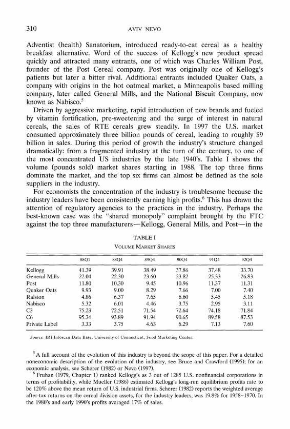
Driven by aggressive marketing, rapid introduction of new brands and fueled by vitamin fortification, pre-sweetening and the surge of interest in natural cereals, the sales of RTE cereals grew steadily. In 1997 the U.S. market consumed approximately three billion pounds of cereal, leading to roughly $9 billion in sales. During this period of growth the industry's structure changed dramatically: from a fragmented industry at the turn of the century, to one of the most concentrated US industries by the late 1940's. Table I shows the volume (pounds sold) market shares starting in 1988. The top three firms dominate the market, and the top six firms can almost be defined as the sole suppliers in the industry.
For economists the concentration of the industry is troublesome because the industry leaders have been consistently earning high profits.6 This has drawn the attention of regulatory agencies to the practices in the industry. Perhaps the best-known case was the "shared monopoly" complaint brought by the FTC against the top three manufacturers-Kellogg, General Mills, and Post-in the
TABLE I
VOLUMEMARKET SHARES
Kellogg General Mills Post Quaker Oats Ralston Nabisco C3 C6 Private Label
Source: I R I Infoscan D a t a Base , University of Connecticut, Food Marketing Center .
' A full account of the evolution of this industry is beyond the scope of this paper. For a detailed noneconomic description of the evolution of the industry, see Bruce and Crawford (1995); for an economic analysis, see Scherer (1982) or Nevo (1997).
Fruhan (1979, Chapter 1) ranked Kellogg's as 3 out of 1285 U.S. nonfinancial corporations in terms of profitability, while Mueller (1986) estimated Kellogg's long-run equilibrium profits rate to be 120% above the mean return of U.S. industrial firms. Scherer (1982) reports the weighted average after-tax returns on the cereal division assets, for the industry leaders, was 19.8% for 1958-1970. In the 1980's and early 1990's profits averaged 17% of sales.
MEASURING MARKET POWER 311
1970's. The focus of that specific complaint was one of the industry's key characteristics: an enormous number of brand^.^ There are currently over 200 brands of RTE cereal, even without counting negligible brands. The brand-level market shares vary from 5% (Kellogg's Corn Flakes and General Mills' Cher- rios) to 1% (the 25th brand) to less than 0.1% (the 100th brand). Not only are there many brands in the industry, but the rate at which new ones are introduced is high and has been increasing over time. From 1950 to 1972 only 80 new brands were introduced. During the 1980's, however, the top six producers introduced 67 new major brands. Somewhat of a side point is that out of these 67 brands only 25 (37 percent) were still on the shelf in 1993.8
Competition by means of advertising was a characteristic of the industry since its early days. Today, advertising-to-sales ratios are about 13 percent, compared to 2-4 percent in other food industries. For the well-established cereal brands, used in the analysis below, the advertising-to-sales ratio is roughly 18 percent. Additional promotional activities are not included in the above ratios. An example of such an activity is manufacturers' coupons, which were widely used in this industry. For more information on coupons and their impact, see Nevo and Wolfram (1999).
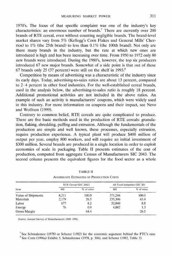
Contrary to common belief, RTE cereals are quite complicated to produce. There are five basic methods used in the production of RTE cereals: granula- tion, flaking, shredding, puffing and extrusion. Although the fundamentals of the production are simple and well known, these processes, especially extrusion, require production experience. A typical plant will produce $400 million of output per year, employ 800 workers, and will require an initial investment of $300 million. Several brands are produced in a single location in order to exploit economies of scale in packaging. Table I1 presents estimates of the cost of production, computed from aggregate Census of Manufacturers SIC 2043. The second column presents the equivalent figures for the food sector as a whole
TABLE I1
AGGREGATE OF PRODUCTIONESTIMATES COSTS
R T E Cereal (SIC 2043) All Food Industries (SIC 20)
Item M % C/o of value MS % of value
Value of Shipments 8,211 100.0 371,246 100.0 Materials 2,179 26.5 235,306 63.4 Labor 677 8.2 32,840 8.8 Energy 76 0.9 4,882 1.3 Gross Margin 64.4 26.5
Solrrce: Annual Survey of Manufacturers 198861992,
See Schmalensee (1978) or Scherer (1982) for the economic argument behind the FTC's case. %ee Corts (1996a) Exhibit 5, Schmalensee (1978, p. 306), and Scherer (1982, Table 3).
AVIV NEVO
TABLE I11
DETAILED OF PRODUC~IONESTIMATES COSTS
% of Mfr % of Retail Item $/lb Price Price
Manufacturer Price Manufacturing Cost:
Grain Other Ingredients Packaging Labor Manufacturing Costs (net of capital costs)"
Gross Margin Marketing Expenses:
Advertising Consumer Promo (mfr coupons) Trade Promo (retail in-store)
Operating Profits
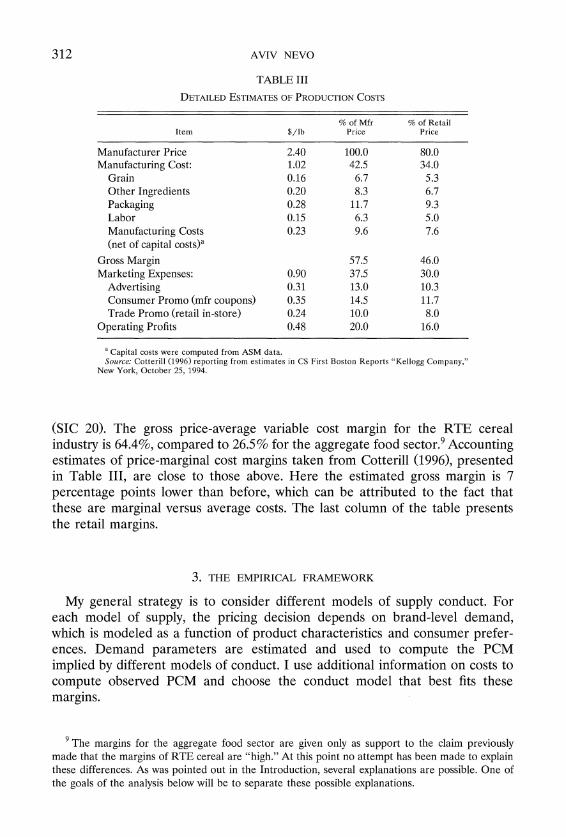
"apital costs were computed from ASM data. Soirrcr: Cotterill (1996) reporting from estimates in CS First Boston Reports "Kellogg Company."
New York, October 25, 1994.
(SIC 20). The gross price-average variable cost margin for the RTE cereal industry is 64.4%, compared to 26.5% for the aggregate food s e ~ t o r . ~ Accounting estimates of price-marginal cost margins taken from Cotterill (1996), presented in Table 111, are close to those above. Here the estimated gross margin is 7 percentage points lower than before, which can be attributed to the fact that these are marginal versus average costs. The last column of the table presents the retail margins.
3. THE EMPIRICAL FRAMEWORK
My general strategy is to consider different models of supply conduct. For each model of supply, the pricing decision depends on brand-level demand, which is modeled as a function of product characteristics and consumer prefer- ences. Demand parameters are estimated and used to compute the PCM implied by different models of conduct. I use additional information on costs to compute observed PCM and choose the conduct model that best fits these margins.
"he margins for the aggregate food sector are given only as support to the claim previously made that the margins of RTE cereal are "high." At this point no attempt has been made to explain these differences. As was pointed out in the Introduction, several explanations are possible. One of the goals of the analysis below will be to separate these possible explanations.

313 MEASURING MARKET POWER
3.1. Supply
Suppose there are F firms, each of which produces some subset, q,of the j = 1,... ,J different brands of RTE cereal. The profits of firm f are
where s,(p) is the market share of brand j , which is a function of the prices of all brands, M is the size of the market, and Cf is the fixed cost of production. Assuming the existence of a pure-strategy Bertrand-Nash equilibrium in prices, and that the prices that support it are strictly positive, the price p, of any product j produced by firm f must satisfy the first-order condition
This set of J equations implies price-costs margins for each good. The markups can be solved for explicitly by defining S,,. = - dsl./dp,, j , r = 1,. . .,J ,
1, i f 3 f : ( r , j ) c q ,
0, otherwise,
and R is a J x J matrix with R,,. = 0; * Sir.In vector notation, the first-order conditions become
s ( p ) - O ( p -mc) = 0,
where s(.), p, and mc are J x 1 vectors of market shares, prices, and marginal- cost, respectively. This implies a markup equation
Using estimates of the demand parameters, we can estimate PCM without observing actual costs, and we can distinguish between three different causes of the markups: the effect due to the differentiation of the products, the portfolio effect, and the effect of price collusion. This is done by evaluating the PCM in three hypothetical industry conduct models. The first structure is that of single-product firms, in which the price of each brand is set by a profit-maximiz- ing agent that considers only the profits from that brand. The second is the current structure, where multi-product firms set the prices of all their products jointly. The final structure is joint profit-maximization of all the brands, which corresponds to monopoly or perfect price collusion. Each of these is estimated by defining the ownership structure, q,and ownership matrix, 0:::.
PCM in the first structure arise only from product differentiation. The difference between the margins in the first two cases is due to the portfolio effect. The last structure bounds the increase in the margins due to price collusion. Once these margins are computed we can choose between the models by comparing the predicted PCM to the observed PCM.
314 AVIV NEVO
3.2. Demand
The exercise suggested in the previous section allows us to estimate the PCM and separate them into different parts. However, it relies on the ability to consistently estimate the own- and cross-price elasticities. As previously pointed out, this is not an easy task in an industry with many closely related products. In the analysis below I follow the approach taken by the discrete-choice literature and circumvent the dimensionality problem by projecting the products onto a characteristics space, thereby making the relevant dimension the dimension of this space and not the number of products.
Suppose we observe t = 1,... ,T markets, each with i = 1,. .. ,Itconsumers. In the estimation below a market will be defined as a city-quarter combination. The conditional indirect utility of consumer i from product j at market t is
where x, is a K-dimensional (row) vector of observable product characteristics, pjt is the price of product j in market t, f j is the national mean valuation of the unobserved (by the econometrician) product characteristics, Atjt is a city-quarter specific deviation from this mean, and sijtis a mean-zero stochastic term. Finally, (a* Pi") are K + 1 individual-specific coefficients.
Examples of observed characteristics are calories, sodium, and fiber content. Unobserved characteristics include a vertical component (at equal prices all consumers weakly prefer a national brand to a generic version) and market- specific effects of merchandising (other than national advertising). I control for the vertical component, f,, by including brand-specific dummy variables in the regressions. Market-specific components are included in At j , and are left as "error terms."1° I assume both firms and consumers observe all the product characteristics and take them into consideration when making decisions.
I model the distribution of consumers' taste parameters for the characteristics as multivariate normal (conditional on demographics) with a mean that is a function of demographic variables and parameters to be estimated, and a variance-covariance matrix to be estimated. Let
where K is the dimension of the observed characteristics vector, Di is a d X 1 vector of demographic variables, 17 is a (K + 1) X d matrix of coefficients that measure how the taste characteristics vary with demographics, and 2 is a scaling matrix. This specification allows the individual characteristics to consist
lo This specification assumes that the unobserved components are common to all consumers. An alternative is to model the distribution of the valuation of the unobserved characteristics, as in Das, Olley, and Pakes (1994). For a further discussion, see Nevo (2000a).
MEASURING MARKET POWER 315
of demographics that are "observed" and additional characteristics that are "unob~erved~~,denoted D, and u, respectively."
The specification of the demand system is completed with the introduction of an "outside good"; the consumers may decide not to purchase any of the brands. Without this allowance a homogeneous price increase (relative to other sectors) of all products does not change quantities purchased. The indirect utility from this outside option is
ulOt= to+ r O D i+ aOviO+ The mean utility of the outside good is not identified (without either making more assumptions or normalizing one of the "inside" goods); thus I normalize to to zero. The coefficients, roand a,, are not identified separately from an intercept, in equation (2), that varies with consumer characteristics.
Let 8 = (O,, 8,) be a vector containing all parameters of the model. The vector 0, = ( a ,p ) contains the linear parameters and the vector 8, = (vet( I l l , vec(2)) the nonlinear parameters.12 Combining equations (2) and (3)
where [p,,, xi] is a ( K + I) x 1vector. The utility is now expressed as the mean utility, represented by a,,, and a mean-zero heteroskedastic deviation from that mean, pijt+ E ~ which captures the effects of the random coefficients. ~~ ,
Consumers are assumed to purchase one unit of the good that gives the highest utility.13 This implicitly defines the set of unobserved variables that lead to the choice of good j. Formally, let this set be
where x are the characteristics of all brands, p,,= (p,,, .. . ,p,,)' and S,,=
(S,,, . . . ,S,,)'. Assuming ties occur with zero probability, the market share of the jth product as a function of the mean utility levels of all the J + 1 goods, given the parameters, is
l1 The distinction between "observed" and "unobserved" individual characteristics refers to auxiliary data sets and not to the main data source, which includes only aggregate quantities and average prices. The distribution of the "observed" characteristics can be estimated from these additional sources.
l2 The reasons for names will become apparent below. 13 A comment is in place about the realism of the assumption that consumers choose no more
than one brand. Many households buy more than one brand of cereal in each supermarket trip but most people consume only one brand of cereal at a time, which is the relevant fact for this modeling assumption. Nevertheless, if one is still unwilling to accept that this is a negligible phenomenon, then this model can be viewed as an approximation to the true choice model. An alternative is to explicitly model the choice of multiple products, or continuous quantities (as in Dubin and McFadden (1984) or Hendel(1999)).
316 AVIV NEVO
where P"(.) denotes population distribution functions. The second equality is a consequence of an assumption of independence of D, u, and r.
By making assumptions on the distribution of the individual attributes, (Di, ui, F ~ , ~ ) , we can compute the integral given in equation (51, either analytically or numerically. Given aggregate quantities and prices, a straightforward estima- tion strategy is to choose parameters that minimize the distance (in some metric) between the market shares predicted by equation ( 5 ) and the observed shares. The actual estimation is slightly more complex because it also has to deal with the correlation between prices and demand shocks, which enter equation ( 5 ) nonlinearly.
A simplifying assumption commonly made in order to solve the integral given in equation ( 5 ) is that consumer heterogeneity enters the model only through the separable additive random shocks, q j I , and that these shocks are distributed i.i.d. with a Type I extreme-value distribution. This assumption reduces the model to the well-known (multinomial) Logit model, which is appealing due to its tractability though it restricts the own- and cross-price elasticities (for details see McFadden (19811, BLP, or Nevo (2000a). The restrictions on the cross-price elasticities, which the Logit assumptions imply are a function only of market shares, are crucial to the exercise conducted below. First, this implies that if, for example, Quaker CapN Crunch (a kids cereal) and Post Grape Nuts (a whole- some simple nutrition cereal) have similar market shares, then the substitution from General Mills Lucky Charms (a kids cereal) toward either of them will be the same. Intuitively, if the price of one kids cereal goes up we would expect more consumers to substitute to another kids cereal than to a nutrition cereal. Yet, the Logit model restricts consumers to substitute towards other brands in proportion to market shares, regardless of characteristics. Second, since the market share of the outside good is very large, relative to the other products, the substitution to the inside goods will on average be downward biased. As I show below this could lead to the wrong conclusions of conduct in this industry.
Slightly less restrictive models, in which the i.i.d. assumption is replaced with a variance components structure, are available (the Generalized Extreme Value model; McFadden (1978)). The Nested Logit model and the Principles of Differentiation Generalized Extreme Value model (Bresnahan, Stern, and Tra- jtenberg (1997)) fall within this class. While less restrictive, both models derive substitution patterns from a priori segmentation.
The full model nests all of these other models and has several advantages over them. First, it allows for flexible own-price elasticities, which will be driven by the different price sensitivity of different consumers who purchase the various products, not by functional-form assumptions about how price enters the indirect utility. Second, since the composite random shock, pijI+ siji, is no longer independent of the product characteristics, the cross-price substitution patterns will be driven by these characteristics. Such substitution patterns are not constrained by a priori segmentation of the market, yet at the same time can take advantage of this segmentation. Furthermore, McFadden and Train (1998) show that the full model can approximate arbitrarily close any choice model. In
MEASURING MARKET POWER 317
particular, the multinomial Probit model (Hausman and Wise (1978)) and the "universal" Logit (McFadden (1981)).
4. DATA AND ESTIMATION
4.1. The Data
The data required to consistently estimate the model previously described consist of the following variables: market shares and prices in each market (in this paper a city-quarter), brand characteristics, advertising, and information on the distribution of demographics.
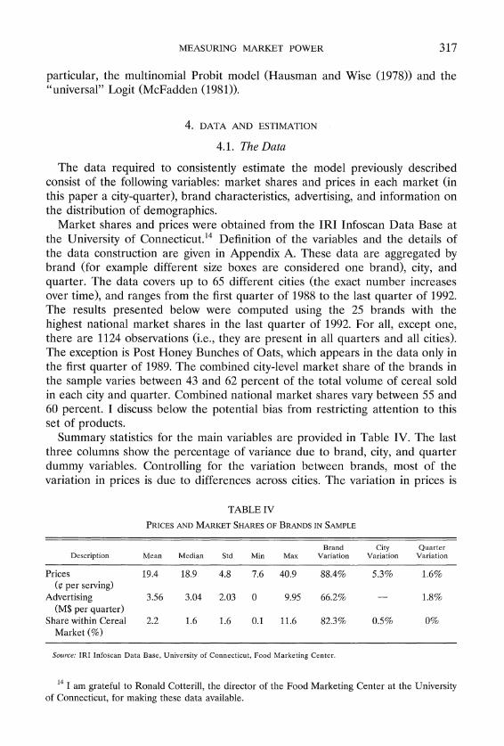
Market shares and prices were obtained from the IRI Infoscan Data Base at the University of Connecticut.14 Definition of the variables and the details of the data construction are given in Appendix A. These data are aggregated by brand (for example different size boxes are considered one brand), city, and quarter. The data covers up to 65 different cities (the exact number increases over time), and ranges from the first quarter of 1988 to the last quarter of 1992. The results presented below were computed using the 25 brands with the highest national market shares in the last quarter of 1992. For all, except one, there are 1124 observations (i.e., they are present in all quarters and all cities). The exception is Post Honey Bunches of Oats, which appears in the data only in the first quarter of 1989. The combined city-level market share of the brands in the sample varies between 43 and 62 percent of the total volume of cereal sold in each city and quarter. Combined national market shares vary between 55 and 60 percent. I discuss below the potential bias from restricting attention to this set of products.
Summary statistics for the main variables are provided in Table IV. The last three columns show the percentage of variance due to brand, city, and quarter dummy variables. Controlling for the variation between brands, most of the variation in prices is due to differences across cities. The variation in prices is
TABLE IV
Description Mean Median Std Min Max Brand
Variation City
Variation Quarter
Varialion
Prices (e per serving)
Advertising (M$ per quarter)
Share within Cereal
19.4
3.56
2.2
18.9
3.04
1.6
4.8
2.03
1.6
7.6
0
0.1
40.9
9.95
11.6
88.4%
66.2%
82.3%
5.3%
-
0.5%
1.6%
1.8%
0% Market (%)
Source: I R I Infoscan Data Base, University of Connecticut, Food Marketing Center
14 I am grateful to Ronald Cotterill, the director of the Food Marketing Center at the University of Connecticut, for making these data available.
318 AVIV NEVO
due to both exogenous and endogenous sources (i.e., variation correlated with demand shocks). Consistent estimation will have to separate these effects. The Infoscan price and quantity data were matched with information on product characteristics and the distribution of individual demographics obtained from the CPS; see Appendix A for details.
4.2. Estimation
I estimate the parameters of the models described in Section 3 using the data described in the previous section by following the algorithm used by BLP. There are three major differences. First, the instrumental variables and the identifying assumptions that support them are different. A somewhat related point, I am able to identify the demand side without specifying a functional form for the supply side, while BLP's identification relies on the functional form of a supply equation. Finally, due to the richness of the data I am able to control for unobserved product characteristics by using brand fixed effects. In this section I outline the estimation; in the next two sections I detail the main differences with BLP.
The key point of the estimation is to exploit a population moment condition that is a product of instrumental variables and a (structural) error term, to form a (nonlinear) GMM estimator. Formally, let Z = [z,, . . . , z,] be a set of instru- ments such that E [ Z ' . w(O*)] = 0, where w, a function of the model parame- ters, is an error term defined below and 8:Venotes the true value of these parameters. The GMM estimate is
(6) 8^= a r g m i n w ( ~ ) ' ~ ~ - ' Z ' w ( 8 ) , e
where A is a consistent estimate of E[Z'ww'Z]. Following Berry (1994), I define the error term as the unobserved product characteristics, [,+ A t j , (or just At,, if brand dummy variables are included). I compute these unobserved characteristics, as a function of the data and parameters, by solving for the mean utility levels, S t , that solve the implicit system of equations
where s,,(.) is the market share function defined by equation (5) , and S,, are the observed market shares. For the Logit model the solution, 6,,(x,p,,, S,,; O,), is equal to ln(S,,) - ln(S,,), while for the full model this inversion is done numeri- cally. Once this inversion has been done, the error term is defined as w,, =
S,,(x,p,,, S,,; 8,) - (x, P + crpIt.). If we want to include brand, time, or city variables they would also be included on the right-hand side. We can now see the reason for distinguishing between 8, and 8,: 6, enters this term, and the GMM objective function, in a linear fashion, while 8, enters nonlinearly.
If brand fixed effects are not included, then the error term is the unobserved product characteristic, [,.However, due to the richness of my data I am able to include brand-specific dummy variables as product characteristics. These dummy
319 MEASURING MARKET POWER
variables include both the mean quality index of observed characteristics, pxj, and the unobserved characteristics, [,. Thus, the error term is the city-quarter specific deviation from the mean valuation, i.e., At j , . The inclusion of brand dummy variables introduces a challenge in estimating the taste parameters, p, which is discussed in Section 4.4.
The weight matrix, A in equation (6), was computed by a two-step procedure. First, I set the weight matrix to Z ' Z and compute an initial estimate of the parameters, denoted 0"). Next, I use this initial estimate to re-compute the weight matrix, i.e., A = (l/n)Cr,, w(0(')) w( o( '))~z'z, where n is the number of observations. Finally, I use the new weight matrix to compute the final esti- mates. I also explored iterating this process several more times, but since the estimated parameters changed only slightly beyond the second iteration, I report only the results from a two-step iteration.
In the Logit model, with the appropriate choice of a weight matrix," this procedure simplifies to two-stage least squares regression of In(Sj,) - In(S,,). In the full random coefficients model, both the computation of the market shares, and the inversion in order to get 6,,(.), have to be done numerically. The value of the estimate in equation (6) is then computed using a nonlinear search. This search is simplified in two ways. First, the first-order conditions of the minimiza- tion problem defined in equation (6) with respect to 0, are linear in these parameters. Therefore, these linear parameters can be solved for (as a function of the other parameters) and plugged into the rest of the first-order conditions, limiting the nonlinear search to only the nonlinear parameters. Second, the results in the paper were computed using a Quasi-Newton method with a user supplied gradient. This was found to work much faster than the Nelder-Mead nonderivative simplex search method used by BLP. For details of the computa- tion algorithm, including a MATLAB computer code, see Nevo (2000a).
Standard errors for the estimates below are computed using the standard formulas (Hansen (1982), Newey and McFadden (1994)). These formulas were corrected for the error due to the simulation process by taking account that the simulation draws are the same for all of the observations in a market. See BLP for further details. Confidence intervals for nonlinear functions of the parame- ters (e.g., own- and cross-price elasticities, as well as markups) were computed by using a parametric bootstrap. I drew repeatedly from the estimated joint distribution of parameters. For each draw I computed the desired quantity, thus generating a bootstrap distribution.
4.3. Instruments
The key identifying assumption in the estimation is the population moment condition, which requires a set of exogenous instrumental variables. In order to understand the need for this assumption, and to understand why (nonlinear)
l5 I.e., A = Z ' Z , which is the "optimal" weight matrix under the assumption of homoscedasticity.

320 AVIV NEVO
least squares estimation will be inconsistent, we examine the pricing decision. By equation (11, prices are a function of marginal costs and a markup term,
This can be decomposed into an overall mean and a deviation from this mean that varies by city and quarter. As pointed out, once brand dummy variables are included in the regression, the error term is the unobserved city-quarter specific deviation from the overall mean valuation of the brand. Since I assumed that players in the industry observe and account for this deviation, it will influence the market-specific markup and bias the estimate of price sensitivity, a , if we use (nonlinear) least squares. Indeed, the results presented in the next section support this.
Much of the previous work16 treats this endogeneity problem by assuming the "location" of brands in the characteristics space is exogenous, or at least predetermined. Characteristics of other products will be correlated with price since the markup of each brand will depend on the distance from the nearest neighbor, and since characteristics are assumed exogenous they are valid IV's. Treating the characteristics as predetermined, rather than reacting to demand shocks, is as reasonable (or unreasonable) here as it was in previous work. However, for our purposes the problem with using observed characteristics to form IV's is much more fundamental. By construction of the data there is no variation in each brand's observed characteristics over time and across cities. The only variation in IV's based on characteristics is a result of differences in the choice set of available brands. While there may be some variation over time due to entry and exit of brands, and across cities due to generic products, the data I have does not capture it. If brand dummy variables are included in the regression the matrix of IV's will be essentially singular.17 A version of this identifying strategy can be used if the brand dummy variables are not included as regressors but are used as IV's instead. Using the brand dummy variables as IV's is a nonparametric way to use all the information contained in the characteristics (if these are fixed). Results from this approach are presented below.
Since this most-commonly-used approach will not work if brand fixed effects are included, I use two alternative sets of instrumental variables in an attempt to separate the exogenous variation in prices (due to differences in marginal costs) and endogenous variation (due to differences in unobserved valuation). First, I use an approach similar to that used by Hausman (1996) and exploit the panel structure of the data. The identifying assumption is that, controlling for brand- specific means and demographics, city-specific valuations are independent across cities (but are allowed to be correlated within a city). Given this assumption, the prices of the brand in other cities are valid IV's. From equation (8) we see that
16 See, for example, Bresnahan (1981, 19871, Berry (19941, BLP (19951, or Bresnahan, Stern, and Trajtenberg (1997).
" It will not be exactly singular because one of the products was not present in all quarters.

321 MEASURING MARKET POWER
prices of brand j in two cities will be correlated due to the common marginal cost, but due to the independence assumption will be uncorrelated with market- specific valuation. One could potentially use prices in all other cities and all quarters as instruments. I use regional quarterly average prices (excluding the city being instrumented) in all twenty quarters.''
There are several plausible situations in which the independence assumption will not hold. Suppose there is a national (or regional) demand shock. For example, the discovery that fiber reduces the risk of cancer. This discovery will increase the unobserved valuation of all fiber-intensive brands in all cities, and the independence assumption will be violated. However, the results below concentrate on well-established brands for which it seems reasonable to assume there are less systematic demand shocks. Also, aggregate shocks to the cereal market will be captured by time dummy variables.
Suppose one believes that local advertising and promotions are coordinated across city borders, but are limited to regions, and that these activities influence demand. Then the independence assumption will be violated for cities in the same region, and prices in cities in the same region will not be valid instrumen- tal variables. However, given the size of the IRI "cities" (which in most cases are larger than MSA's) and the size of the Census regions, this might be less of a problem. The size of the IRI city determines how far the activity has to go in order to cross city borders; the larger the city, the smaller the chance of correlation with neighboring cities. Similarly, the larger the Census region the less likely is correlation with all cities in the region. Finally, the IRI data are used by the firms in the industry; thus it is not unlikely that they base their strategies on a city-level geographic split.
Determining how plausible are these, and possibly other situations, is an empirical issue. I approach it by examining another set of instrumental variables that attempts to proxy for the marginal costs directly and compare the differ- ence between the estimates implied by the different sets of IV's. The marginal costs include production (materials, labor, and energy), packaging, and distribu- tion costs. Direct production and packaging costs exhibit little variation and are too small a percentage of marginal costs to be correlated with prices. Also, except for small variations over time, a brand dummy variable, which is included as one of the regressors, proxies for these costs. The last component of marginal costs, distribution costs, includes the cost of transportation, shelf space, and labor. These are proxied by region dummy variables, which pick up transporta- tion costs; city density, which is a proxy for the difference in the cost of space; and average city earnings in the supermarket sector computed from the CPS Monthly Earning Files.
A persistent regional shock for certain brands will violate the assumption underlying the validity of these IV's. If, for example, all western states value natural cereals more than east-coast states, region-specific dummy variables will
l8 There is no claim made here with regards to the "optimality" o f these IV's. A potentially interesting question might be are there other ways o f weighting the information from different cities.
322 AVIV NEVO
be correlated with the error term. However, in order for this argument to work the difference in valuation of brands has to be above and beyond what is explained by demographics and heterogeneity since both are controlled for.
4.4. Brand-SpecificDummy Variables
As previously pointed out, one of the main differences between this paper and previous work is the inclusion of brand-specific dummy variables as product characteristics. There are at least two good reasons to include these dummy variables. First, in any case where we are unsure that the observed characteris- tics capture the true factors that determine utility, fixed effects should be included in order to improve the fit of the model. Note that this helps fit the mean utility level, a(.), while substitution patterns are still driven by observed characteristics (either physical characteristics or market segmentation), as is the case if we were not to include brand fixed effects.
Furthermore, a major motivation (Berry (1994)) for the estimation scheme previously described is the need to instrument for the correlation between prices and the unobserved quality of the product, tj. A brand-specific dummy variable captures the characteristics that do not vary by market, namely, xip + tj. Therefore, the correlation between prices and the unobserved quality is fully accounted for and does not require an instrument. In order to introduce brand-specific dummy variables we require observations on more than one market. However, even without these dummy variables, fitting the model using observations from a single market is difficult (BLP, footnote 30).
There are two potential objections to the use of brand dummy variables. First, the main motivation for the use of discrete-choice models was to reduce the dimensionality problem. Introducing brand fixed effects increases the number of parameters only with J (the number of brands) and not J ~ .Thus we have not defeated the purpose of using a discrete-choice model. Furthermore, the brand- specific intercepts enter as part of the linear parameters and do not increase the computational difficulty.
In order to retrieve the taste coefficients, p, when brand fixed-effects are included, I regress the estimated brand effects on the characteristics, as in the minimum-distance procedure proposed by Chamberlain (1982). Formally, let d denote the J X 1vector of brand dummy coefficients, X be the J X K (K <J ) matrix of product characteristics, and 5 be the J X 1 vector of unobserved product attributes. Then from (2)
d = X p + [ .
If we assume that E[51x1= 0,'"he estimates of p and 5 are
p = ( ~ J V ; ~ X ) - ~ X ' V ; ' ~ , t = C i - x p ,
19 This is the assumption required to justify the use of observed characteristics as IV's. Here, unlike previous work, this assumption is used only to recover the taste parameters and does not impact the estimates of price sensitivity.
MEASURING MARKET POWER 323
where d^ is the vector of coefficients estimated from the procedure described in the previous section, and Vd is the covariance matrix of these estimates. This is simply a GLS regression where the independent variable consists of the esti- mated brand effects, estimated using the GMM procedure previously described and the full sample. The number of "observations" in this regression is the number of brands. The correlation in the values of the dependent variable is treated by weighting the regression by the estimated covariance matrix, I/,, which is the estimate of this correlation. The coefficients on the brand dummy variables provide an "unrestricted" estimate of mean utility. The minimum- distance estimator projects these estimates onto a lower K-dimensional space, which is implied by a "restricted" model that sets 5 to zero. Chamberlain provides a chi-squared test to evaluate these restrictions.
5. RESULTS
5.1. Logit Results
As pointed out in Section 3, the Logit model yields restrictive and unrealistic substitution patterns, and therefore is inadequate for measuring market power. Nevertheless, due to its computational simplicity it is a useful tool in getting a feel for the data. In this section I use the Logit model to examine: (a) the importance of instrumenting for price; and (b) the effects of the different sets of instrumental variables discussed in the previous section.
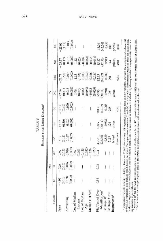
Table V displays the results obtained by regressing In(Sj,) - In(So,) on prices, advertising expenditures, brand and time dummy variables. In columns (i)-(iii) I report the results of ordinary least squares regressions. The regression in column (i) includes observed product characteristics, but not brand fixed effects, and therefore the error term includes the unobserved product characteristic, tj.'O The regressions in columns (ii) and (iii) include brand dummy variables and therefore fully control for t,. The effects of including brand-specific dummy variables on the price and advertising coefficients are significant both statisti- cally and economically. However, even the coefficient on price given in column (iii) is relatively low. The Logit demand structure does not impose a constant elasticity, and therefore the estimates imply a different elasticity for each brand-city-quarter combination. The mean of the distribution of own-price elasticities across the 27,862 observations is -1.53 (the median is - 1.50) with a standard deviation of 0.39, and 5.5% of the observations are predicted to have inelastic demand.
Columns (iv)-(x) of Table V use various sets of instrumental variables in two-stage least squares regressions. The first set of results, presented in column (iv), is based on the same specification as column (i) but uses brand dummy variables as IV's. This is similar to the identification assumptions used by much
20 The unreported coefficients on the product characteristics are (s.e.1: constant, -4.44 (0.041, fatcal, 0.17 (0.041, sugar, 2.7 (0.091, mushy, -0.12 (0.011), fiber, 0.04 (0.061, all family segment, 0.53 (0.021, kids segment, 0.47 (0.021, health segment, 0.53 (0.02).

325 MEASURING MARKET POWER
of the previous work (see Section 4.3). Indeed, compared to column (i) the price coefficient has nearly doubled, but it is almost identical to the coefficients from the OLS regression which includes brand dummy variables as regressors.
Column (v) uses the average regional prices in all twenty quarters21 as instrumental variables in a two-stage least squares regression. Not surprisingly, the coefficient on price increases and the estimated demand curves for all brand-city-quarter combinations are elastic (the mean of the distribution is -3.38, the median is -3.30, and the standard deviation is 0.85). Column (vi) uses a different set of IV's: the proxies for city level marginal costs. The coefficient on price is similar in the two regressions.
The similarity between the estimates of the price coefficient continues to hold when we introduce demographics into the regression. Columns (vii)-(viii) pre-sent the results from the previous two sets of IV7s, while column (vi) presents an estimation using both sets of instruments jointly. The addition of demographics increases the absolute value of the price coefficient, leading to an increase in the absolute value of the price elasticity. As we recall from the previous section, if there are regional demand shocks, then both sets of IV's are not valid. City-specific valuations may be a function of demographics, and if demographics are correlated within a region these valuations will be correlated. Under this story, adding demographics eliminates the omitted-variable bias and improves the over-identification test statistic. The coefficients on demographics capture the change in the value of the cereal relative to the outside option as a function of demographics. The results suggest that the value of cereals increases with income, while age and household size are nonsignificant. Demographics could potentially be added to the regression in a more complex manner (for example, allowing for interactions with the product characteristics), but since the purpose of the Logit model is mainly descriptive, this is done only in the full model. Finally, column (x) allows for city-specific intercepts, which control even further for city-level demand shocks. The results in this column are again almost identical to the previous results.22
The first stage R-squared and F-statistic for all the instrumental variable regressions are high, suggesting (although not promising) that the IV's have some power. The first-stage regressions are presented in Appendix B. With the exception of the last column, the tests of over-identification are rejected, suggesting that the identifying assumptions are not valid. However, it is unclear whether the large number of observations is the reason for the rejectionz3 or that the IV's are not valid. Once city fixed effects are included, as in column (x), the instruments are no longer rejected. Combined with the fact that the coefficients did not change between columns (ix) and (x), I interpret this as
The results are essentially the same if I use only the regional average price for that quarter. 22 Furthermore, by adding city fixed effects to the regression we demonstrate that we have
enough variation in the time dimension to identify the parameters, and the results are not driven purely by cross-sectional differences.
23 It is well known that with a large enough sample a chi-squared test will reject essentially any model.
326 AVIV NEVO
evidence that although the city effects improve the fit of the model, excluding them from the regression does not seem to bias the coefficients. Furthermore, if I am able to control for demographics in a more elaborate way, then the validity of the instrumental variables cannot be rejected. The full model controls for demographics in a more complete manner and as I claim below approximates the city fixed effects model.
The regressions also include advertising, which has a statistically significant coefficient. With the exception of column (i) the estimated effect of advertising is roughly the same in all specifications. The large coefficient in column (i) is a result of the correlation between unobserved characteristics and advertising: brands with larger market shares tend to have higher ej's and also advertise more. Once we control for this potential e n d ~ g e n e i t y ~ ~ the mean elasticity with respect to advertising is approximately 0.06,which seems low. A Dorfman-Steiner condition requires advertising elasticities to be an order of magnitude higher. This is probably a result of measurement error in the advertising data. Nonlin- ear effects in advertising were also tested and were found to be insignificant.
The price-cost margins implied by the estimates are given in the first column of Table VIII. A discussion of these results is deferred to later in the paper. The important thing to take from these results is the similarity between estimates using the two sets of IV's, and the importance of controlling for demographics and heterogeneity. The similarity between the coefficients does not promise the two sets of IV's will produce identical coefficients in different models or that these are valid IV's. However, I believe that with proper control for demograph- ics and heterogeneity, as in the full model, these are valid IV's.
5.2. Results porn the Full Model
The estimates of the full model are based on equation (4) and were computed using the procedure described in Section 4.2. Predicted market shares are computed using equation (5) and are based on the empirical distribution of demographics (as sampled from the March C P S ) , ~ ~ independent normal distri- butions (for u) , and Type I extreme value (for 8).The IV's include both average
24 In the previous sections I have focused my attention to the endogeneity of prices but little was said about the endogeneity of advertising. Conventional wisdom of this industly and these results might cast doubt on this decision. I wish to point out several things. First, advertising varies by brand-quarter, and not by city, thus, potentially is less correlated with the errors. Second, I do not use the advertising coefficient in the analysis below; therefore, as long as bias, if it exists, in this coefficient does not impact the price elasticities there is no effect on the conclusions reached below. Once I add brand fixed effects, the IV's used to instrument for price seem to have no effect on the advertising coefficient, suggesting that the opposite might also be true (i.e., that instrumenting for advertising would have little, or no, impact on estimates of price sensitivity).
25 I sampled 40 individuals for each year, in total 200 for each city. For some cities the CPS did not sample more than 40 individuals in some years. I tried increasing the number of individuals when possible and the results were robust. I also used the methods of Imbens and Lancaster (1994) to make the samples more representative, but since the qualitative results did not change I do not report these specifications.
327 MEASURING MARKET POWER
TABLE VI
RESULTSFROM THE FULLMODEL^
Standard Interaction? with Demographic Variables Means Deviations
Variablc ( p ' s ) (v 's) Incume Illcomc Sq Age Child
Price
Advertising
Constant
Cal from Fat
Sugar
Mushy
Fiber
All-family
Kids
Adults
GMM Objective (degrees of freedom) MD X 2
% of Price Coefficients > 0
"Based on 27,862 obrervations. Except where noted, parameters are GMM estimates. All regrersionr include brand and time dummy variables. Arymptotically robust rtandard errors are given in parentherer.
"stimater from a minimum-dirtance procedure.
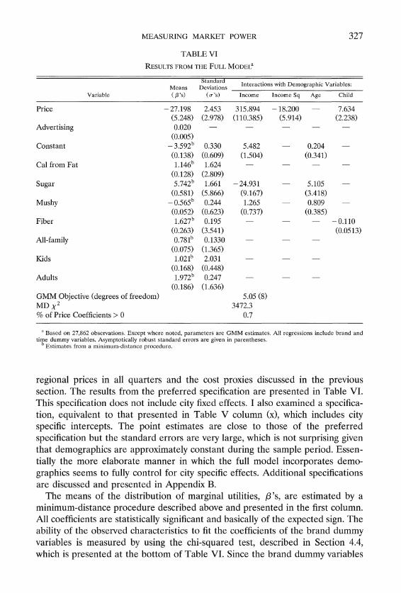
regional prices in all quarters and the cost proxies discussed in the previous section. The results from the preferred specification are presented in Table VI. This specification does not include city fixed effects. I also examined a specifica- tion, equivalent to that presented in Table V column (x), which includes city specific intercepts. The point estimates are close to those of the preferred specification but the standard errors are very large, which is not surprising given that demographics are approximately constant during the sample period. Essen- tially the more elaborate manner in which the full model incorporates demo- graphics seems to fully control for city specific effects. Additional specifications are discussed and presented in Appendix B.
The means of the distribution of marginal utilities, P's, are estimated by a minimum-distance procedure described above and presented in the first column. All coefficients are statistically significant and basically of the expected sign. The ability of the observed characteristics to fit the coefficients of the brand dummy variables is measured by using the chi-squared test, described in Section 4.4, which is presented at the bottom of Table VI. Since the brand dummy variables
328 AVIV NEVO
are estimated very precisely (due to the large number of observations) it is not surprising that the restricted model is rejected.
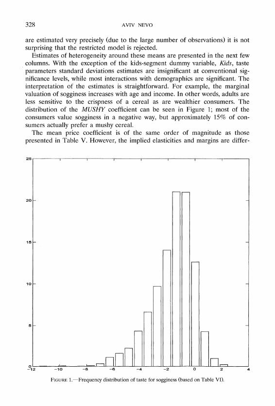
Estimates of heterogeneity around these means are presented in the next few columns. With the exception of the kids-segment dummy variable, Kids, taste parameters standard deviations estimates are insignificant at conventional sig- nificance levels, while most interactions with demographics are significant. The interpretation of the estimates is straightforward. For example, the marginal valuation of sogginess increases with age and income. In other words, adults are less sensitive to the crispness of a cereal as are wealthier consumers. The distribution of the MUSHY coefficient can be seen in Figure 1; most of the consumers value sogginess in a negative way, but approximately 15% of con-sumers actually prefer a mushy cereal.
The mean price coefficient is of the same order of magnitude as those presented in Table V. However, the implied elasticities and margins are differ-
FIGURE1.-Frequency distribution of taste for sogginess (based on Table VI).
MEASURING MARKET POWER 329
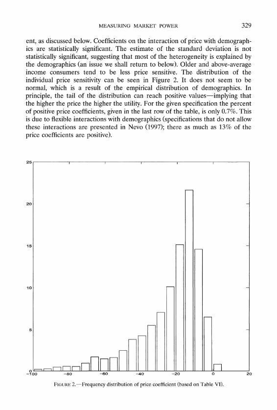
ent, as discussed below. Coefficients on the interaction of price with demograph- ics are statistically significant. The estimate of the standard deviation is not statistically significant, suggesting that most of the heterogeneity is explained by the demographics (an issue we shall return to below). Older and above-average income consumers tend to be less price sensitive. The distribution of the individual price sensitivity can be seen in Figure 2. It does not seem to be normal, which is a result of the empirical distribution of demographics. In principle, the tail of the distribution can reach positive values-implying that the higher the price the higher the utility. For the given specification the percent of positive price coefficients, given in the last row of the table, is only 0.7%. This is due to flexible interactions with demographics (specifications that do not allow these interactions are presented in Nevo (1997); there as much as 13% of the price coefficients are positive).
FIGURE2.-Frequency distribution of price coefficient (based on Table VI).
330 AVIV NEVO
As noted above, all the estimates of the standard deviations are statistically insignificant, suggesting that the heterogeneity in the coefficients is mostly explained by the included demographics. A measure of the relative importance of the demographics and random shocks can be obtained from the ratios of the variance explained by the demographics to the total variation in the distribution of the estimated coefficients; these are over 90%.26,27 Appendix B presents the results of a specification that sets the random shocks, u,, to zero.
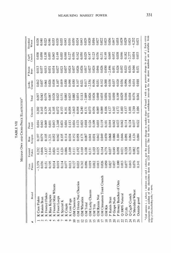
Table VII presents a sample of estimated own- and cross-price elasticities. Each entry i, j, where i indexes row and j column, gives the elasticity of brand i with respect to a change in the price of j. Since the model does not imply a constant elasticity, this matrix will be different depending on what values of the variables are used to evaluate it. Rather than choosing a particular value (say the average, or a value at a particular market), I present the median of each entry over the 1124 markets in the sample. The results are intuitive. For example, Lucky Charms, a kids cereal, is most sensitive to a change in the price of Corn Pops and Froot Loops, also kids cereals. At the same time it is least sensitive to a change in the price of cereals like Corn Flakes, Total, or Wheaties, all cereals aimed at different market segments. These substitution patterns are persistent across the table.
An additional diagnostic of how far the results are from the restrictive form imposed by the Logit model is given by examining the variation in the cross-price elasticities in each column. As discussed in Section 2, the Logit model restricts all elasticities within a column to be equal. Therefore, an indicator of how well the model has overcome these restrictions is to examine the variation in the estimated elasticities. One such measure is given by examining the ratio of the maximum to the minimum cross-price elasticity, within a column (the Logit model implies that all cross-price elasticities within a column are equal and therefore have a ratio of one). This ratio varies from 21 (Corn Flakes) to 3.5 (Shredded Wheat), with a 95% confidence intervals of 11-260 and 3-52 respec- tively. Not only does this tell us the results have overcome the Logit restrictions, but more importantly it suggests for which brands the characteristics do not
"Rossi, McCulloch, and Allenby (1996) find that using previous purchasing histoly helps explain heterogeneity above and beyond what is explained by demographics alone. Berry, Levinsohn, and Pakes (1998) reach a similar conclusion using second choice data. The results of this paper do not suggest that previous purchases or second choices would have no value; they only suggest that the data reject the assumed normal distribution. This result is not driven by the aggregate data and would probably continue to hold for a number of other parametric distributions (ICiser (1996)).
"Unlike previous work (for example BLP), by construction I have very little variation across markets in the choice set. If it is variation in the choice set that is identifying the variance of the random shocks, then it is not surprising that my estimates are insignificant. This explanation does not explain why the point estimates are low (as opposed to the standard-errors being high) and why the impact of demographic variables is significant.
MEASURING MARKET POWER
332 AVIV NEVO
seem strong enough to overcome the restrictions. This test therefore suggests which characteristics we might want to add.28
Finally, the bottom row of Table VII presents the elasticity of the share of the outside good with respect to the price of the "inside" goods. By comparing the ratio of these elasticities to the average in each column we see the relative importance of the outside good to each brand. For example, the cross-price elasticity of the outside good is higher for Kellogg's Corn Flakes than Froot Loops. Not only is it higher in absolute terms, but it is higher as a ratio of the average cross-price elasticity in that column.29 Once again this is an intuitive result. Generic versions of Kellogg's Corn Flakes have higher market shares than generic versions of Froot Loops. All generic products are included in the outside good and therefore it should not be surprising that the outside good is more sensitive to the price of Corn Flakes.
5.3. Price-Cost Margins
Predicted PCM
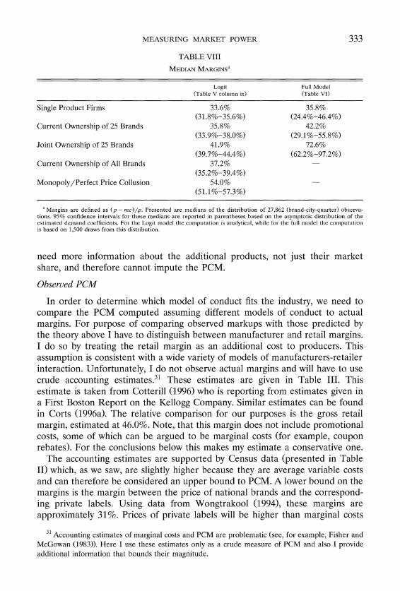
Given the demand parameters estimated in the previous sections, we can use equation (1) to compute PCM for different conduct models. As explained in Section 3.1, I compute PCM for three hypothetical industry structures, thus placing bounds on the importance of the different causes for PCM. Table VIII presents the median PCM for the Logit and the full models using the demand estimates of Tables V and VI. Different rows present the PCM that the three models of pricing conduct predict. In principle each brand-city-quarter combina- tion will have a different predicted margin. The figures in the table are the median of these 27,862 numbers.30
Although the mean price sensitivity estimated from the full model, given in Table VI, is similar to the price coefficient estimated in the Logit model, given in Table V, the implied markups are different. Since the full model does a better job of estimating the cross-price elasticities, it is not surprising that the differ- ence increases as we go from single, to multi-product firms, and then to joint ownership of the 25 brands used in the estimation. For the Logit model we can use the estimates to compute the predicted PCM for brands that were not included in the estimation. All we need is the price sensitivity, estimated from the sample, and the market shares of additional brands. In the full model we
"A formal specification test of the Logit model (in the spirit of Hausman and McFadden (1984) is the test of the hypothesis that all the nonlinear parameters are jointly zero. This hypothesis is easily rejected.
29 comparing the absolute value of the elasticities across columns is somewhat meaningless, since in each column the absolute price change is different. In order to compare across columns semi-elasticities, or the percent change in market share due to say a 10 cents change in price, need to be computed.
30 Medians rather than means are presented to eliminate the sensitivity to outliers. Computing the means of the distribution with the 5% tails truncated yields essentially identical results.
MEASURING MARKET POWER 333
TABLE VIII
MEDIANMARGINS"
Logit Full Model (Table V column 1x1 (Table VI)
Single Product Firms 33.6% (31.8%-35.6%)
Current Ownership of 25 Brands 35.8% (33.9%-38.0%)
Joint Ownership of 25 Brands 41.9% (39.7%-44.4%)
Current Ownersllip of All Brands 37.2% (35.2%-39.4%)
Monopoly/Perfect Price Collusion 54.0% (51.1%-57.3%)
"Margins are defined as ( p - nic)/p. Presented are medians of the dlstributlon of 27.862 (brand-city-quarter) observn- tions. 95% confidence inte~vals for these medlans are reported In parentheses based on the asymptotic distr~bution of the estimated demand coefficients. For the Logit model the computation is analytical, while for the full model the computation is based on 1.500 draws from this distribution.
need more information about the additional products, not just their market share, and therefore cannot impute the PCM.
Observed PCM
In order to determine which model of conduct fits the industry, we need to compare the PCM computed assuming different models of conduct to actual margins. For purpose of comparing observed markups with those predicted by the theory above I have to distinguish between manufacturer and retail margins. I do so by treating the retail margin as an additional cost to producers. This assumption is consistent with a wide variety of models of manufacturers-retailer interaction. Unfortunately, I do not observe actual margins and will have to use crude accounting estimates3' These estimates are given in Table 111. This estimate is taken from Cotterill (1996) who is reporting from estimates given in a First Boston Report on the Kellogg Company. Similar estimates can be found in Corts (1996a). The relative comparison for our purposes is the gross retail margin, estimated at 46.0%. Note, that this margin does not include promotional costs, some of which can be argued to be marginal costs (for example, coupon rebates). For the conclusions below this makes my estimate a conservative one.
The accounting estimates are supported by Census data (presented in Table 11) which, as we saw, are slightly higher because they are average variable costs and can therefore be considered an upper bound to PCM. A lower bound on the margins is the margin between the price of national brands and the correspond- ing private labels. Using data from Wongtrakool (1994), these margins are approximately 31%. Prices of private labels will be higher than marginal costs
31 Accounting estimates of marginal costs and PCM are problematic (see, for example, Fisher and McGowan (1983)). Here I use these estimates only as a crude measure of PCM and also I provide additional information that bounds their magnitude.
334 AVIV NEVO
for several reasons. First, they also potentially include a markup term, but lower than the national brands. Second, the private label manufacturers might have different marginal costs, most likely higher. For these reasons this margin is only a lower bound on PCM.
Testing the Models
The accounting estimates of marginal costs and the implied margins are a crude estimate for the "typical" brand. Nevertheless, the PCM predicted by the different models are different enough that this crude measure can still be used to separate the different effects. Using the confidence intervals provided in Table VIII we can reject the null hypothesis that either the "typical" margins, presented in Table 111, or the bounds, discussed in the previous section, are equal to those predicted by the model of joint profit maximization for the 25 brands. Furthermore, we cannot reject the null hypothesis that these quantities are consistent with the prediction of the multi-product Nash-Bertrand equilib- rium.
One might wonder how restricting the analysis to the top 25 brands alters the results and conclusion. In principle the estimates of price sensitivity should not be biased by this sample selection, and indeed some analysis performed with different samples suggests this is the case. Therefore, the only potential differ- ences are in the margins computed in Table VIII. As previously noted, in order to compute the quantities given in the table for more brands in the full model, these brands have to be part of the sample. Since this is somewhat infeasible I will argue that the likely outcome of including more brands is to strengthen the conclusions. It is more probable that the smaller brands, not included in the sample, have a higher, in absolute value, own-price elasticity (relative to similar brands that are in the sample) and therefore the PCM predicted by the first model will go down. This effect will be completely offset if, rather than giving equal weight to all brands, we weight the observations by market shares (the market-share-weighted mean equivalents of the results in Table VIII are roughly 2-3 percentage points higher, which is the likely effect of including smaller brands). For the other two models there is an additional effect. Including more products in the "inside" goods rather than the "outside" good will tend to increase the predicted PCM. The more products included, the larger the effect, which implies that the effect on the fully collusive model will be larger. An idea of the potential increase can be seen by examining the Logit results. The effects for the full model are likely to be even larger. This implies that the PCM predicted by the multi-product Nash-Bertrand model are likely to be even closer to observed quantities, while the PCM predicted by the collusive model will be even further. In this sense the results of Table VIII are conservative.
There are at least two alternative testing methods that have been previously used in similar situations. First, a strategy that has been successfully used in homogeneous-goods industries is to define conduct parameters that measure the degree of competition (Bresnahan (1989)). In addition to the problems associ- ated with how one should interpret these parameters (see, for example, Costs

MEASURING MARKET POWER 335
(1999)), the identification requirements for this strategy are unlikely to be met in differentiated-product industries (Nevo (1998)). The second alternative is to construct a formal test of nonnested hypotheses (for example, Bresnahan (1987) or Gasmi, Laffont, and Vuong (1992)). These methods require evaluating the likelihood of each model, which can be derived only after making additional assumptions. In particular, I would have to make assumptions on the distribu- tion of the error terms and fully define a supply equation. Not only are both nontrivial assumptions, but based on the data and the unrestricted specification used here there seems to be no natural set of assumptions to make.
Finally, as a side note I would like to point out that using the same test procedure proposed here and the Logit estimates, displayed in the first column of Table VIII, would yield dramatically different results. Using the Logit results one cannot reject the mode of full collusion over all products. This result is completely driven by the strong assumptions of the Logit model discussed above, and is not an indication of conduct in the industry.
5.4. Additional Specifications and a Final Word About Endogeneity
Section 5.2 presented in detail the preferred specification. Some additional specifications are presented in Appendix B and more can be found in Nevo (1997). Overall it is important to note that even though these specifications are different in some aspects from the preferred specification, the conclusions described in the previous section are robust. In addition to the various specifi- cations within the framework used here I also examined the multi-stage demand system, which has recently been used by Hausman, Leonard, and Zona (1994) and Hausman (1996). Despite some interesting differences in the pattern of estimated cross-price substitution, the conclusions reached in the previous section are unchanged. A full presentation, discussion, and comparison of the results is beyond the scope of this paper (for details, see Nevo (1997)).
In addition to the work mentioned in the previous paragraph various other authors have also studied the RTE cereal industry. Hausman (1996) explores the value of a new brand of cereal by estimating a multi-level demand system using a weekly panel of brand-level sales and prices in seven cities. His estimation exploits the time variation in the weekly prices to identify the demand parame- ters. Thus despite the fact that I follow Hausman in using prices in other cities as IV, our estimation strategies are different. From his results one can estimate the effects computed in the previous section. The conclusions are essentially identical. Kiser (1996) and Shum (1999) use household-level rather than aggre- gate data to estimate demand for Although these data might also yield inconsistent estimates, the reasons are different than here. Therefore it is
32 Kiser (1996) estimates a random coefficients discrete clloice model, similar to the one used in this paper, to compute the potential gains to firms from being able to price discriminate among consumers. Sllum (1999) estimates a nested Logit model to examine the impact of advertising on demand. His focus is on testing whether advertising increases product differentiation, by creating brand loyalty, or decreases it, by encouraging switching among brands.
336 AVIV NEVO
encouraging that the estimated own- and cross-price elasticities are very similar to those produced here. All of these studies use different data sets and different identifying assumptions than those used here. However, they all imply similar conclusions, which increases the confidence in the results.
This paper uses a random coefficients discrete choice (mixed Logit) model to estimate a brand-level demand system for RTE cereal. Parameter identification exploits the panel structure of the data, and is based on an independence assumption of demand shocks across cities for each brand. The estimates are supported by different identifying assumptions. The estimated elasticities are used to compute price cost margins that would prevail under different conduct models. These different models are tested by comparing the predictions to crude observed measures of margins. A Nash-Bertrand pricing game, played between multi-product firms (as the firms in the industry are), is found to be consistent with observed price-cost margins. Furthermore, it seems that if any significant price collusion existed, the observed margins would have been much higher. If we are willing to accept Nash-Bertrand as a benchmark of noncollusive pricing, we are left to conclude, unlike previous work, that even with PCM greater than 45%, prices in the industry are not a result of collusive behavior.
The results rule out an extreme version of cooperative pricing, one in which all firms jointly maximize profits. There is a continuum of models that are not tested here. For example, the results in this paper do not rule out cooperative pricing between a subset of products (say Kellogg's and Post Raisin Bran) or producers (say Post and Nabisco). The methods and test used here could deal with these additional models but would require more detailed cost data.
Most economists are familiar with this industry from the research of Schmalensee (1978), which lays out the economic argument at the foundation of the FTC's "shared monopoly" case against the industry in the 1970's. Even though the standard description of the complaint will include a claim of cooperative pricing, the core of the case was brand proliferation and its use as a barrier to entry, not cooperative pricing. As much as I would like to claim that this paper proves or disproves the FTC's case, I cannot do so. I find that the high observed PCM are primarily due to the firms' ability to maintain a portfolio of differentiated brands and influence the perceived quality of these brands by means of advertising. In a sense my analysis suggests that, whether right or wrong, the FTC's claim focused on the important dimensions of competition. In order to make claims regarding the anti-competitive effects of brand introduc- tion and advertising one would have to extend the model to deal with these dimensions explicitly.
Understanding the form of price competition has at least two immediate uses. Structural models of demand and supply have recently gained popularity for analysis of mergers. These models rely on estimates of demand and assumptions about pre- and post-merger equilibrium to predict the effects of a merger. Nevo
MEASURING MARKET POWER 337
(1999) uses the model, data, and results of this paper for such an analysis. A different application of the results and methods of this paper is to welfare analysis. For example, Hausman (1996) uses estimates of demand and assump- tions about short-run price competition to evaluate the welfare gains from introduction of new goods. His analysis computes the virtual price of a brand prior to introduction, i.e., the lowest price that sets the demand for a product equal to zero given the prices of other brands. The virtual price is then used to compute a price index. The analysis relies on obtaining consist estimates of demand parameters and correctly specifying the model of competition. The results and conclusions of this paper can be used as arguments for or against the assumptions used in such an analysis.
Dept. of Economics, Uniuersity of California, Berkeley, 549 Euans Hall #3880, Berkeley, CA94720-3880,U.S.A.; neuo@econ. berkeley. edu; http:// elsa. berkeley. edu/ - neuo / .
Manuscript receiued October; 1997;final reuision receiced Janzlar): 2000.
APPENDIX A: DATA
Data
The data described in Section 4 were obtained from various sources. Quantity and price data were obtained from the Food Marketing Policy Center at the University of Connecticut. These data were collected by Information Resources, Inc. (IRI), a marketing firm in Chicago, using scanning devices in a national random sample of supermarkets located in various metropolitan areas and rural towns. Weekly data for UPC-coded products are drawn from a sample which represents the universe of supermarkets with annual sales of more than $2 million dollars, accounting for 82% of grocery sales in the US. In most cities the sample covers more than 20% of the relevant population, and due to the importance of the sample to its customers, IRI makes an effort to make the sample representative. This is confirmed by unpublished analysis conducted by the BLS.
Market shares are defined by converting volume sales into number of servings and dividing by the total potential number of servings in a city in a quarter. This potential was assumed to be one serving per capita per day. The market share of the outside good was defined as the difference between one and the sum of the inside goods market shares. A price variable was created by dividing the dollar sales by the number of servings sold, and was deflated using a regional urban consumer CPI. The dollar sales reflect the price paid by consumers at the register, generating an average real per-serving transaction price. However, the sales data do not account for any manufacturers' coupons.
Advertising data were taken from the Leading National Advertising data base, which contains quarterly national advertising expenditures by brand collected from 10 media sources.34 I used the total of the 10 types of media.
33 This was done by using the serving weight suggested by the manufacturer, which is assumed correct (or at least proportional to the "true" serving weight).
34 The sources include: magazines, Sunday magazines, newspapers, outdoor, network television, spot television, syndicated television, cable networks, network radio, and national spot radio.
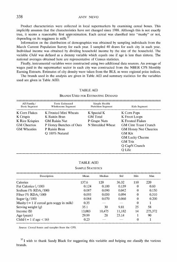
338 AVIV NEVO
Product characteristics were collected in local supermarkets by examining cereal boxes. This implicitly assumes that the characteristics have not changed since 1988. Although this is not exactly true, it seems a reasonable first approximation. Each cereal was classified into "mushy" or not, depending on its sogginess in milk.35
Information on the distribution of demographics was obtained by sampling individuals from the March Current Population Survey for each year. I sampled 40 draws for each city in each year. Individual income was obtained by dividing household income by the size of the household. The variable Child was defined as a dummy variable which equals one if age is less than sixteen. The national averages obtained here are representative of Census statistics.
Finally, instrumental variables were constructed using two additional data sources. An average of wages paid in the supermarket sector in each city was constructed from the NBER CPS Monthly Earning Extracts. Estimates of city density were taken from the BLS, as were regional price indices.
The brands used in the analysis are given in Table A(I) and summary statistics for the variables used are given in Table A(I1).
TABLE A(I)
All Family/ Taste Enhanced Simple Heal th Basic Segment Wholesome Segment Nutrition Segment Kids Segment
K Corn Flakes K Frosted Mini Wheats K Special K K Corn Pops K Crispix K Raisin Bran GM Total K Froot Loops K Rice Krispies GM Raisin Nut P Grape Nuts K Frosted Flakes GM Cheerios P Honey Bunches of Oats N Shredded Wheat GM Cinn Toast Crunch GM Wheaties P Raisin Bran GM Honey Nut Cheerios
Q 100% Natural GM Kix GM Lucky Charms GM Trix Q CapN Crunch Q Life
TABLE A(I1)
SAMPLESTATISTICS
Description M e a n Median Std blin Max
Calories Fat Calories (/loo) Sodium (% RDA/100) Fiber (% RDA/100) Sugar (g/100) Mushy (= 1 if cereal gets soggy in milk) Serving weight (g) Income ($1 Age (years) Child (= 1 if age < 16)
Sour.ce: Cereal boxes and samples from the CPS
35 I wish to thank Sandy Black for suggesting this variable and helping me classify the various brands.
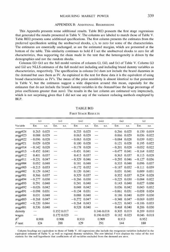
MEASURING MARKET POWER 330
APPENDIX B: ADDITIONAL REGRESSIONS
This Appendix presents some additional results. Table B(1) presents the first stage regressions that generated the results presented in Table V. The columns are labeled to match those of Table V. Table B(I1) presents some additional specifications. The first column presents the estimates from the preferred specification setting the unobserved shocks, c,'s, to zero for some of the characteristics. The estimates are essentially unchanged, as are the estimated margins, which are presented at the bottom of the table. This similarity continues to hold if I set the unobserved shocks to zero for all characteristics, thus supporting the claim made in the text that the heterogeneity is driven by the demographics and not the random shocks.
Columns (ii)-(iv) are the full model version of columns (i), (iii), and (iv) of Table V. Column (ii) and (iii) are NLLS estimates of the full model not including and including brand dummy variables as characteristics, respectively. The specification in column (iv) does not include the brand dummies in the demand but uses them as IV. As explained in the text for these data it is the equivalent of using brand characteristics as IV's. The mean of the price sensitivity is almost identical to that presented in Table V, but the estimates suggest a wide dispersion around this mean, especially for the estimates that do not include the brand dummy variables in the demand (see the large percentage of price coefficients greater than zero). The results in the last column are estimated very imprecisely, which is not surprising given that I did not use any of the variance reducing methods employed by BLP.
TABLE B(1)
FIRST STAGE RESULTS
(v) (vi) (vii) (viii) (ix) (x)
Variable Est. s.e. Est. s.e. Est, s.e. Est, s.e. Est. s.e. Est. s.e.
avgp924 avgp923 avgp922 avgp921 avgp914 avgp913 avgp912 avgp911 avgp904 avgp903 avgp902 avgp901 avgp894 avgp893 avgp892 avgp891 avgp884 avgp883 avgp882 avgp881 density wages R F-test
Column headings are equivalent to those of Table V. All regressions also include the exogenous variables included in the equivalent columns of Table V, as well as regional dummy variables. The row labeled F-test displays the value of the test statistic for the null hypothesis that coefficients of all variables excluded from the demand are zero.
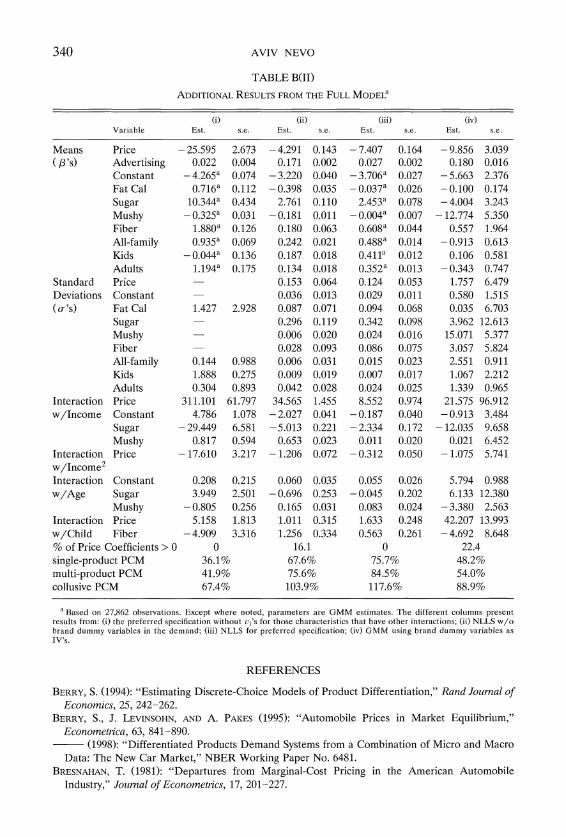
340 AVIV NEVO
TABLE B(I1)
ADDITIONAL FROM THE FULL MODEC' RESULTS
(i) (11) (IV) Variahle Est. s.e Es t s e Est s e
Means Price -25.595 2.673 -4.291 0.143 -9.856 3.039 ( P 's) Advertising 0.022 0.004 0.171 0.002 0.180 0.016
Constant -4 . 2 6 5 9 . 0 7 4 -3.220 0.040 -5.663 2.376 Fat Cal 0.716" 0.112 -0.398 0.035 -0,100 0.174 Sugar 1 0 . 3 4 4 9 . 4 3 4 2.761 0.110 -4.004 3.243 Mushy -0.325" 0.031 -0.181 0.011 - 12.774 5.350 Fiber 1.880" 0.126 0.180 0.063 0.557 1.964 All-family 0 . 9 3 5 V . 0 6 9 0.242 0.021 -0.913 0.613 I d s -0.044".136 0.187 0.018 0.106 0.581 Adults 1.194" 0.175 0.134 0.018 -0.343 0.747
Standard Price - 0.153 0.064 1.757 6.479 Deviations Constant - 0.036 0.013 0.580 1.515 (a 's) Fat Cal 1.427 2.928 0.087 0.071 0.035 6.703
Sugar - 0.296 0.119 3.962 12.613 Mushy - 0.006 0.020 15.071 5.377
-Fiber 0.028 0.093 3.057 5.824 All-family 0.144 0.988 0.006 0.031 2.551 0.911 Kids 1.888 0.275 0.009 0.019 1.067 2.212 Adults 0.304 0.893 0.042 0.028 1.339 0.965
Interaction Price 311.101 61.797 34.565 1.455 21.575 96.912 w/Income Constant 4.786 1.078 -2.027 0.041 -0.913 3.484
Sugar -29.449 6.581 -5.013 0.221 - 12.035 9.658 Mushy 0.817 0.594 0.653 0.023 0.021 6.452
Interaction Price - 17.610 3.217 - 1.206 0.072 - 1.075 5.741 w/1ncome2 Interaction Constant 0.208 0.215 w/Age Sugar 3.949 2.501
Mushy -0.805 0.256 Interaction Price 5.158 1.813 w/Child Fiber -4.909 3.316 % of Price Coefficients > 0 0 single-product PCM 36.1% multi-product PCM 41.9% collusive PCM 67.4%
" B a s e d on 27.862 observations. Except where noted, parameters are GMM estimates. T h e different columns present results from: (i) the preferred specification without i,,'s for those characteristics tha t have o ther interactions; (ii) NLLS w / o hrand dummy variables in the demand; (iii) NLLS for preferred specification; (iv) GMM using hrand dummy variables as IV's.
REFERENCES
BERRY, S. (1994): "Estimating Discrete-Choice Models of Product Differentiation," Rand Jo~rrnal of' Economics, 25, 242-262.
BERRY, S., J. LEVINSOHN, A. PAKES (1995): "Automobile Prices in Market Equilibrium,"AND
Econor?zetruca,63, 841-890. -(1998): "Differentiated Products Demand Systems from a Combination of Micro and Macro
Data: The New Car Market," NBER Working Paper No. 6481. BRESNAHAN,T. (1981): "Departures from Marginal-Cost Pricing in the American Automobile
Industry," Jo~rrnal of'Econometrics, 17, 201-227.
MEASURING MARKET POWER 341
----- (1987): "Competition and Collusion in the American Automobile Oligopoly: The 1955 Price War," Journal of Industrial Economics, 35, 457-482.
----- (1989): "Empirical Methods for Industries with Market Power," in Handboolc of Industrial Organization, Vol. 11, ed. by R. Schmalensee and R. Willig. Amsterdam: North-Holland.
BRESNAHAN,T., S. STERN, AND M. TRAJTENBERG (1997): "Market Segmentation and the Sources of Rents from Innovation: Personal Computers in the Late 1980's," RAND Journal of Econonlics, 28, S17-S44.
BRUCE, S., AND B. CRAWFORD (1995): Cerealizing America. Boston: Faber and Faber. CARDELL,N. S. (1989): "Extensions of the Multinomial Logit: The Hedonic Demand Model, The
Non-Independent Logit Model, and the Ranked Logit Model," Ph.D. Dissertation, Harvard University.
CHAMBERLAIN,G. (1982): "Multi Variate Regression Models for Panel Data," Journal ofEcorzomet- rics, 18, 5-46.
CORTS, K. S. (1996a): "The Ready-to-Eat Breakfast Cereal Indust~y in 1994 (A)," Halyard Business School Case Number N9-795-191.
-- (1999): "Conduct Parameters and the Measurement of Market Power," Journal of Economet- rics, 88, 227-250.
COTTERILL,R. W. (1996): "High Cereal Prices and the Prospects for Relief by Expansion of Private Label and Antitrust Enforcement," Testimony offered at the Congressional Forum on the Performance of the Cereal Industry, Washington, D.C., March 12.
DAS, S., S. OLLEY, AND A. PAKES (1994): "Evolution of Brand Qualities of Consumer Electronics in the U.S.," mimeo.
DUBIN,J., AND D. MCFADDEN (1984): "An Econometric Analysis of Residential Electric Appliance Holding and Consumption," Econometrica, 52, 345-362.
FISHER,F. M., AND J. J. MCGOWAN(1983): "On the Misuse of Accounting Rates of Return to Infer Monopoly Profits," American Economic Reuiew, 73, 82-97.
FRUHAN,W. H. (1979): Financial Stmtegy: Studies in the Creation, Transfer, and Destrzlction of Shareholder Value. Homewood, IL: Irwin.
GASMI,F., J. J. LAFFONT,AND Q. VUONG (1992): "Econometric Analysis of Collusive Behavior in a Soft-Drink Market," Journal ofEconomics and Management Strategy, 1, 277-311.
HANSEN, L. (1982): "Large Sample Properties of Generalized Method of Moments Estimators," Econometrica, 50, 1029-1054.
HAUSMAN,J. (1983): "Specification and Estimation of Simultaneous Equations Models," in Hanrl-book of Econometrics, ed, by Z. Griliches and M. Intiligator. Amsterdam: North-Holland. -(1996): "Valuation of New Goods Under Perfect and Imperfect Competition," in The
Economics of New Goods, Studies in Income and Wealth Vol. 58, ed. by T. Bresnahan and R. Gordon. Chicago: National Bureau of Economic Research.
HAUSMAN, AND J. D. ZONA (1994). "Competitive Analysis with Differentiated J., G. LEONARD, Products," Annales D'Economie et de Statistique, 34, 159-180.
HAUSMAN, (1984): "Specification Tests for the Multinomial Logit Model," J., AND D. MCFADDEN Econometrica, 52, 1219-1240.
HAUSMAN,J., AND D. WISE (1978): "A Conditional Probit Model for Qualitative Choice: Discrete Decisions Recognizing Interdependence and Heterogeneous Preferences," Econonzetrica, 49, 403-426.
HENDEL,I. (1999): "Estimating Multiple Discrete Choice Models: An Application to Computeriza- tion Returns," Re~'iew of Ecolzonzic Studies, 66, 423-446.
IMBENS, G., AND T. LANCASTER Micro and Macro Data in Microeconomic (1994): "Combining Models," Reuiew of Economic Studies, 61, 655-680.
KISER, E. K. (1996): "Heterogeneity in Price Sensitivity: Implications for Price Discrimination," mimeo, University of Wisconsin-Madison.
MCFADDEN,D. (1973): "Conditional Logit Analysis of Qualitative Choice Behavior," in Frontiers of Econonzetrics, ed. by P. Zarembka. New York: Academic Press.
----- (1978): "Modeling the Choice of Residential Location," in Spatial Irzteraction Tlleory and Planning Models, ed. by A. Karlgvist, et al. Amsterdam: North-Holland.
342 AVIV NEVO
---- (1981): "Econometric Models of Probabilistic Choice," in StrztcturalArzalysis ofDiscrzte Data, ed. by C. Manski and D. McFadden. Cambridge: MIT Press, pp. 198-272.
MCFADDEN, (1998): "Mixed MNL Models for Discrete Response," University of D., AND K. TRAIN California at Berkeley, mimeo (available at http://emlab.berkeley.edu/ - train).
MUELLER,D. C. (1986): Profits in tlze Long Run. Cambridge: Cambridge University Press. NEVO, A. (1997): "Demand for Ready-to-Eat Cereal and Its Implications for Price Competition,
Merger Analysis, and Valuation of New Goods," Ph.D. Dissertation, Harvard University. ---- (1998): "Identification of the Oligopoly Solution Concept in a Differentiated-Products
Industry," Econonzics Letters, 59, 391-395. -(2000a): "A Practitioner's Guide to Estimation of Random Coefficients Logit Models of
Demand," Journal of Econonzics and Managenzerzt Strategv, 9, 513-548. ---- (2000b): "Mergers with Differentiated Products: The Case of the Ready-to-Eat Cereal
Industiy," The RAND Jozournal of Economics, 31, 395-421. NEVO, A,, AND C. WOLFRAM (1999): "Prices and Coupons for Breakfast Cereals," NBER Working
Paper No. 6932. NEWEY,W., AND D. MCFADDEN (1994): "Estimation in Large Samples," in The Handbooli of
Ecorlonzetrics, Vol. 4, ed. by D. McFadden and R. Engle. Amsterdam: North-Holland. Ross~, P., R. E. MCCULLOCH, (1996): "The Value of Purchase Histoiy Data in AND G. M. ALLENBY
Target Marketing," Marketing Science, 15, 321-340. SCHERER,F. M. (1982): "The Breakfast Cereal Industry," in The Structure ofAtnericarz Inclzrstry, ed.
by W. Adams. New York: Macmillan. SCHMALENSEE,R. (1978): "Entry Deterrence in the Ready-to-Eat Breakfast Cereal Industry," Bell
Journal of Econonzics, 9, 305-327. SHUM,M. (1999): "Advertising and Switching Behavior in the Breakfast Cereal Market," University
of Toronto, mimeo (available at http://www.chass.utoronto.ca/eco/eco.html). WONGTRAKOOL,B. (1994): "An Assessment of the Cereal Killers: Private Labels in the Ready-to-Eat
Cereal Indust~y," Senior Thesis, Harvard University.

You have printed the following article:
Measuring Market Power in the Ready-to-Eat Cereal IndustryAviv NevoEconometrica, Vol. 69, No. 2. (Mar., 2001), pp. 307-342.Stable URL:
http://links.jstor.org/sici?sici=0012-9682%28200103%2969%3A2%3C307%3AMMPITR%3E2.0.CO%3B2-3
This article references the following linked citations. If you are trying to access articles from anoff-campus location, you may be required to first logon via your library web site to access JSTOR. Pleasevisit your library's website or contact a librarian to learn about options for remote access to JSTOR.
[Footnotes]
3 Competition and Collusion in the American Automobile Industry: The 1955 Price WarTimothy F. BresnahanThe Journal of Industrial Economics, Vol. 35, No. 4, The Empirical Renaissance in IndustrialEconomics. (Jun., 1987), pp. 457-482.Stable URL:
http://links.jstor.org/sici?sici=0022-1821%28198706%2935%3A4%3C457%3ACACITA%3E2.0.CO%3B2-D
3 Estimating Discrete-Choice Models of Product DifferentiationSteven T. BerryThe RAND Journal of Economics, Vol. 25, No. 2. (Summer, 1994), pp. 242-262.Stable URL:
http://links.jstor.org/sici?sici=0741-6261%28199422%2925%3A2%3C242%3AEDMOPD%3E2.0.CO%3B2-Z
3 Automobile Prices in Market EquilibriumSteven Berry; James Levinsohn; Ariel PakesEconometrica, Vol. 63, No. 4. (Jul., 1995), pp. 841-890.Stable URL:
http://links.jstor.org/sici?sici=0012-9682%28199507%2963%3A4%3C841%3AAPIME%3E2.0.CO%3B2-U
13 An Econometric Analysis of Residential Electric Appliance Holdings and ConsumptionJeffrey A. Dubin; Daniel L. McFaddenEconometrica, Vol. 52, No. 2. (Mar., 1984), pp. 345-362.Stable URL:
http://links.jstor.org/sici?sici=0012-9682%28198403%2952%3A2%3C345%3AAEAORE%3E2.0.CO%3B2-Y
http://www.jstor.org
LINKED CITATIONS- Page 1 of 5 -
NOTE: The reference numbering from the original has been maintained in this citation list.
16 Competition and Collusion in the American Automobile Industry: The 1955 Price WarTimothy F. BresnahanThe Journal of Industrial Economics, Vol. 35, No. 4, The Empirical Renaissance in IndustrialEconomics. (Jun., 1987), pp. 457-482.Stable URL:
http://links.jstor.org/sici?sici=0022-1821%28198706%2935%3A4%3C457%3ACACITA%3E2.0.CO%3B2-D
16 Estimating Discrete-Choice Models of Product DifferentiationSteven T. BerryThe RAND Journal of Economics, Vol. 25, No. 2. (Summer, 1994), pp. 242-262.Stable URL:
http://links.jstor.org/sici?sici=0741-6261%28199422%2925%3A2%3C242%3AEDMOPD%3E2.0.CO%3B2-Z
16 Market Segmentation and the Sources of Rents from Innovation: Personal Computers in theLate 1980sTimothy F. Bresnahan; Scott Stern; Manuel TrajtenbergThe RAND Journal of Economics, Vol. 28, No. 0, Special Issue in Honor of Richard E. Quandt.(1997), pp. S17-S44.Stable URL:
http://links.jstor.org/sici?sici=0741-6261%281997%2928%3CS17%3AMSATSO%3E2.0.CO%3B2-R
25 Combining Micro and Macro Data in Microeconometric ModelsGuido W. Imbens; Tony LancasterThe Review of Economic Studies, Vol. 61, No. 4. (Oct., 1994), pp. 655-680.Stable URL:
http://links.jstor.org/sici?sici=0034-6527%28199410%2961%3A4%3C655%3ACMAMDI%3E2.0.CO%3B2-S
26 The Value of Purchase History Data in Target MarketingPeter E. Rossi; Robert E. McCulloch; Greg M. AllenbyMarketing Science, Vol. 15, No. 4. (1996), pp. 321-340.Stable URL:
http://links.jstor.org/sici?sici=0732-2399%281996%2915%3A4%3C321%3ATVOPHD%3E2.0.CO%3B2-7
28 Specification Tests for the Multinomial Logit ModelJerry Hausman; Daniel McFaddenEconometrica, Vol. 52, No. 5. (Sep., 1984), pp. 1219-1240.Stable URL:
http://links.jstor.org/sici?sici=0012-9682%28198409%2952%3A5%3C1219%3ASTFTML%3E2.0.CO%3B2-V
http://www.jstor.org
LINKED CITATIONS- Page 2 of 5 -
NOTE: The reference numbering from the original has been maintained in this citation list.

31 On the Misuse of Accounting Rates of Return to Infer Monopoly ProfitsFranklin M. Fisher; John J. McGowanThe American Economic Review, Vol. 73, No. 1. (Mar., 1983), pp. 82-97.Stable URL:
http://links.jstor.org/sici?sici=0002-8282%28198303%2973%3A1%3C82%3AOTMOAR%3E2.0.CO%3B2-L
References
Estimating Discrete-Choice Models of Product DifferentiationSteven T. BerryThe RAND Journal of Economics, Vol. 25, No. 2. (Summer, 1994), pp. 242-262.Stable URL:
http://links.jstor.org/sici?sici=0741-6261%28199422%2925%3A2%3C242%3AEDMOPD%3E2.0.CO%3B2-Z
Automobile Prices in Market EquilibriumSteven Berry; James Levinsohn; Ariel PakesEconometrica, Vol. 63, No. 4. (Jul., 1995), pp. 841-890.Stable URL:
http://links.jstor.org/sici?sici=0012-9682%28199507%2963%3A4%3C841%3AAPIME%3E2.0.CO%3B2-U
Competition and Collusion in the American Automobile Industry: The 1955 Price WarTimothy F. BresnahanThe Journal of Industrial Economics, Vol. 35, No. 4, The Empirical Renaissance in IndustrialEconomics. (Jun., 1987), pp. 457-482.Stable URL:
http://links.jstor.org/sici?sici=0022-1821%28198706%2935%3A4%3C457%3ACACITA%3E2.0.CO%3B2-D
Market Segmentation and the Sources of Rents from Innovation: Personal Computers in theLate 1980sTimothy F. Bresnahan; Scott Stern; Manuel TrajtenbergThe RAND Journal of Economics, Vol. 28, No. 0, Special Issue in Honor of Richard E. Quandt.(1997), pp. S17-S44.Stable URL:
http://links.jstor.org/sici?sici=0741-6261%281997%2928%3CS17%3AMSATSO%3E2.0.CO%3B2-R
http://www.jstor.org
LINKED CITATIONS- Page 3 of 5 -
NOTE: The reference numbering from the original has been maintained in this citation list.

An Econometric Analysis of Residential Electric Appliance Holdings and ConsumptionJeffrey A. Dubin; Daniel L. McFaddenEconometrica, Vol. 52, No. 2. (Mar., 1984), pp. 345-362.Stable URL:
http://links.jstor.org/sici?sici=0012-9682%28198403%2952%3A2%3C345%3AAEAORE%3E2.0.CO%3B2-Y
On the Misuse of Accounting Rates of Return to Infer Monopoly ProfitsFranklin M. Fisher; John J. McGowanThe American Economic Review, Vol. 73, No. 1. (Mar., 1983), pp. 82-97.Stable URL:
http://links.jstor.org/sici?sici=0002-8282%28198303%2973%3A1%3C82%3AOTMOAR%3E2.0.CO%3B2-L
Large Sample Properties of Generalized Method of Moments EstimatorsLars Peter HansenEconometrica, Vol. 50, No. 4. (Jul., 1982), pp. 1029-1054.Stable URL:
http://links.jstor.org/sici?sici=0012-9682%28198207%2950%3A4%3C1029%3ALSPOGM%3E2.0.CO%3B2-O
Specification Tests for the Multinomial Logit ModelJerry Hausman; Daniel McFaddenEconometrica, Vol. 52, No. 5. (Sep., 1984), pp. 1219-1240.Stable URL:
http://links.jstor.org/sici?sici=0012-9682%28198409%2952%3A5%3C1219%3ASTFTML%3E2.0.CO%3B2-V
Panel Data and Unobservable Individual EffectsJerry A. Hausman; William E. TaylorEconometrica, Vol. 49, No. 6. (Nov., 1981), pp. 1377-1398.Stable URL:
http://links.jstor.org/sici?sici=0012-9682%28198111%2949%3A6%3C1377%3APDAUIE%3E2.0.CO%3B2-3
Combining Micro and Macro Data in Microeconometric ModelsGuido W. Imbens; Tony LancasterThe Review of Economic Studies, Vol. 61, No. 4. (Oct., 1994), pp. 655-680.Stable URL:
http://links.jstor.org/sici?sici=0034-6527%28199410%2961%3A4%3C655%3ACMAMDI%3E2.0.CO%3B2-S
http://www.jstor.org
LINKED CITATIONS- Page 4 of 5 -
NOTE: The reference numbering from the original has been maintained in this citation list.
The Value of Purchase History Data in Target MarketingPeter E. Rossi; Robert E. McCulloch; Greg M. AllenbyMarketing Science, Vol. 15, No. 4. (1996), pp. 321-340.Stable URL:
http://links.jstor.org/sici?sici=0732-2399%281996%2915%3A4%3C321%3ATVOPHD%3E2.0.CO%3B2-7
http://www.jstor.org
LINKED CITATIONS- Page 5 of 5 -
NOTE: The reference numbering from the original has been maintained in this citation list.