Measuring Liquidity Mismatch in the Banking Sector · PDF fileMeasuring Liquidity Mismatch in...

Measuring Liquidity Mismatchin the Banking Sector

Jennie Bai, Arvind Krishnamurthy, Charles-Henri Weymuller ∗

August 2014

Abstract

This paper implements a liquidity measure proposed by Brunnermeier, Gorton and Krishnamurthy (2011),"Liquidity Mismatch Index (LMI)," to measure the mismatch between the market liquidity of assets andthe funding liquidity of liabilities. We construct the LMI for 2870 bank holding companies during 2002 -2013 and investigate its time-series and cross-sectional patterns. The aggregate LMI worsens from less than[negative] $1 trillion in 2002 to $3.3 trillion in 2008, before reversing back to pre-crisis level in 2009. In the crosssection, we find that banks with more liquidity mismatch (i) experience more negative stock returns duringthe crisis, but more positive returns in non-crisis periods; (ii) experience more negative stock returns on eventscorresponding to a liquidity run, and more positive returns on events corresponding to government liquidityinjection; (iii) borrow more from the government during the financial crisis.

JEL Classification: G21, G28.Keywords: liquidity mismatch; liquidity regulation; market liquidity; funding liquidity.

∗We thank Viral Acharya, Allen Berger, Christa Bouwman, Markus Brunnermeier, Dong Beom Choi, Adam Copeland,Michael Fleming, Antoine Martin, Klaus Schaeck, and seminar participants at the Federal Reserve Bank of New York, Bankof France, Bank of England, the Department of the Treasury’s Office of Financial Research, European Bank Association’s5th Annual Financial Stability Conference at Tilburg, Georgetown University, Copenhagen Business School, University ofRhode Island, for helpful comments. Jonathan Choi provided excellent research assistance. Bai is with McDonough School ofBusiness at Georgetown University, [email protected]. Krishnamurthy is with Stanford University Graduate Schoolof Business and NBER, [email protected]. Weymuller is with Harvard University, [email protected].

1

mailto:[email protected]



Measuring Liquidity Mismatch in the Banking Sector

Abstract

This paper implements a liquidity measure proposed by Brunnermeier, Gorton and

Krishnamurthy (2011), "Liquidity Mismatch Index (LMI)," to measure the mismatch between the

market liquidity of assets and the funding liquidity of liabilities. We construct the LMI for 2870 bank

holding companies during 2002 - 2013 and investigate its time-series and cross-sectional patterns.

The aggregate LMI worsens from less than [negative] $1 trillion in 2002 to $3.3 trillion in 2008,

before reversing back to pre-crisis level in 2009. In the cross section, we find that banks with more

liquidity mismatch (i) experience more negative stock returns during the crisis, but more positive

returns in non-crisis periods; (ii) experience more negative stock returns on events corresponding

to a liquidity run, and more positive returns on events corresponding to government liquidity

injection; (iii) borrow more from the government during the financial crisis.

1

1 Introduction

Liquidity plays an enormous role in financial crises. Fleming (2012) notes that across its many liquidity

facilities, the Federal Reserve provided over $1.5 trillion of liquidity support during the crisis. The

number is much higher if one includes other forms of government liquidity support such as lending

by the Federal Home Loan Bank – lending to banks peaks at $1 trillion in September 2008 – or the

Federal Deposit Insurance Corporation guarantees – insurance limits are increased in the crisis, and

the guarantees are extended to $336 billion of bonds as of March 2009 (He, Khang, and Krishnamurthy

(2010)). Recognizing the importance of liquidity in the crisis, the Basel III committee has proposed

regulating the liquidity of commercial banks. Yet, despite its importance there is no consensus on how

to measure liquidity. Indeed, the only consensus is that liquidity is a slippery concept and is hard to

measure.

This paper implements a liquidity measure proposed by Brunnermeier, Gorton, and

Krishnamurthy (2011, 2012). Their "Liquidity Mismatch Index" (LMI) measures the mismatch between

the market liquidity of assets and the funding liquidity of liabilities, at a firm level. There are many

empirical challenges that arise in implementing their theoretical measure. We take up these challenges

and design a procedure to implement the LMI that relies on balance-sheet as well as off-balance-sheet

information of a given bank and market indicators of liquidity and liquidity premia. We construct

the LMI for the universe of bank holding companies (BHCs) in the U.S. and describe features of the

time-series and cross-sectional properties of the bank-specific and aggregate LMI.

What makes a good liquidity measure? First, we argue that a liquidity measure should be useful for

macro-prudential purposes. It should measure liquidity imbalances in the financial system, offering

an early indicator of financial crises. It should also quantitatively describe the liquidity condition of

the financial sector, and the amount of liquidity the Fed may be called upon to provide in a financial

crisis. The LMI performs well on these metrics. An important aspect of the LMI is that it can be be

aggregated across banks to measure the liquidity mismatch of a group of banks or the entire financial

sector. Liquidity measures which are based on ratios, such as Basel’s liquidity coverage ratio, do not

possess this aggregation property. Our aggregate LMI as shown in Figure 3 indicates an accumulating

liquidity mismatch over the period from 2002 to 2007. In 2007 Q1, the LMI is about (negative) $2.2

1

trillion. Thus, had the LMI been computed in 2007, the Fed would have expected that in the event of

an aggregate liquidity crisis, it may need to provide $2.2 trillion of liquidity to completely mitigate the

liquidity-run aspect of the financial crisis.1 Moreover, the LMI reverses course from 2008 to mid-2009,

coincident with the Fed’s liquidity injections, returning to its 2002 level. Finally, we show that the LMI

methodology can naturally be used to administer a liquidity stress test by a regulator, and present the

results of such a stress test at various time points.

Our second benchmark arises from micro considerations. We argue that an efficient liquidity

measure should describe liquidity risk in the cross-section of banks, identifying which banks carry

the most liquidity risk. We show that our measure performs well in this dimension. When market-

wide liquidity conditions deteriorate, a firm with a worse LMI should be more negatively affected. We

examine the cross-section of banks and show that banks with a worse LMI have lower stock returns

during the 2008 financial crisis. We also find that across event dates corresponding to a worsening

of liquidity conditions, the low LMI banks experience more negative stock returns. Across event

dates corresponding to an increase in Fed liquidity provision, the low LMI banks experience more

positive stock returns. Our cross-sectional analysis also reveals interesting patterns in the way that

firms manage liquidity. We find that banks with high liquidity mismatch (low LMI value) have high

stock returns before and after the crisis, when aggregate liquidity conditions were good. Moreover,

we find that the banks that have the lowest LMI (i.e. the most liquidity shortfall) are the largest

banks, perhaps suggesting a strategy of exploiting the too-big-to-fail backstop. We also find that the

banks with the most negative LMI, measured before the crisis, borrow the most from Federal Reserve

facilities and receive the largest TARP injections. The LMI thus helps to describe the cross-section of

liquidity risk in the financial sector. For regulatory purposes, the cross-sectional LMI can help identify

systemically important institutions, but here using a liquidity metric.

These two dimensions, the macro and the micro, appear to us to be the most important dimensions

on which to evaluate a liquidity measure. One contribution of the paper is to offer these metrics. This

is particularly important going forward because there are in principal many ways to measure liquidity

1One theoretical rationale to justify liquidity injections by the Fed is an inter-bank market freeze, as modelled in Acharyaand Skeie (2011). Another reason is the stigma of borrowing at the discount window. See Ennis and Weinberg (2012) for a asignaling model of this stigma. A liquidity injection also prevents coordination failures that can lead to bank insolvency, asin fundamental bank runs models a la Rochet and Vives (2004).

2

and what is needed are benchmarks that can be used to discriminate across measures.

Related Literature

Our paper is related to a small literature on how to measure liquidity. On the practitioner

side, there are a number of different metrics that firms use to manage liquidity, ranging from the

accounting ‘quick’ ratio to more sophisticated measures. On the policy side, several central bank

studies including Banerjee (2012), de Haan and End (2012) investigate measures for bank liquidity

regulation in response to Basel III. The pioneering paper in the academic literature is Berger and

Bouwman (2009), which is the first paper to recognize the importance of measuring liquidity and

propose a theoretically-motivated liquidity measure. Berger and Bouwman (2009) measure the

liquidity mismatch at the bank level and explore the cross-sectional and time-series properties of this

liquidity mismatch measure. The principal theoretical difference between the LMI and the Berger-

Bouwman measure is that the LMI incorporates information from market measures of liquidity and

liquidity premia.2 In the language of Berger and Bouwman, our liquidity weights are time-varying,

while their liquidity weights are only asset and liability specific. Time variation in these liquidity

weights is important in capturing liquidity stress during a financial crisis. Another contribution of

our paper is in discussing and evaluating the LMI against the benchmarks we have suggested. These

benchmarks are important because they help us to calibrate the liquidity weights, which are hard to

pin down on purely theoretical grounds.

There is also a banking and corporate finance literature that explores the determinants of liquidity

holdings on a firm’s balance sheet, for example, Heider, Hoerova, and Holhausen (2009), Acharya

and Merrouche (2013) and Acharya and Rosa (2013). In most of this literature, liquidity is defined

as the cash or liquid assets held on the asset side of the balance sheet. In our approach, liquidity is

constructed from both asset and liability side of the balance sheet (as in Berger and Bouwman (2009)),

and is furthermore dependent on market-wide liquidity conditions. Each asset and each liability

contributes to the liquidity position of the bank. We leave it for future work to revisit this literature

using our more comprehensive liquidity measure.

In comparing the stock returns of banks that hold more liquidity on their balance sheet to those

2There is an alternative measure in Berger and Bouwman (2009) that sets the weights on bank loans to vary with theamount of securitization. In our paper, the time-varying feature is generalized to every item on and off balance sheet.

3

holding less liquidity, we find that the former underperform during non-crisis periods. This may be

because holding liquidity is on average costly, carrying insurance benefits that are only reaped in crisis

periods (as in Holmstrom and Tirole (1998)). It will be interesting to link our findings with a welfare

analysis and study the benefits and costs of holding liquidity. It will also be interesting to see if our

empirical analysis offers clarity on the optimal regulation of bank liquidity (see e.g., Stein (2013)).

The paper proceeds as follows. The next section builds up a theoretical model for the liquidity

mismatch measure and Section 3 constructs the empirical measure. Section 4 evaluates the LMI in the

macro dimension while Section 5 evaluates the LMI in the micro dimension. Section 6 concludes the

paper and discuss future work.

2 Liquidity Mismatch Index: Theoretical Framework

The Liquidity Mismatch Index (LMI) of Brunnermeier, Gorton, and Krishnamurthy (2011, 2012)

provides one approach to measure a bank’s liquidity. They define the LMI as the “cash equivalent

value" of a firm in a given state assuming that:

i Counterparties act most adversely. That is, parties that have contracts with the firm act to extract

as much cash as possible from the firm under the terms of their contracts. This defines the

liquidity promised through liabilities.

ii The firm computes its best course of action, given the assumed stress event, to raise as much

cash against its balance sheet as it can to withstand the cash withdrawals. That is, the firm

computes how much cash it can raise from asset sales, pre-existing contracts such as credit

lines, and collateralized loans such as repo backed by assets currently held by the firm. The

computation assumes that the firm is unable to raise unsecured debt or equity. The total cash

raised is the asset-side liquidity.

Central to this definition is that liquidity is computed based on a scenario where counterparties

act most adversely. To understand why the worst-case is appropriate, consider defining liquidity for

a hypothetical Diamond-Dybvig bank that is subject to a bank run. Suppose that the bank owns 100

4

long-term illiquid assets where early liquidation generates 50. The bank is financed by 75 of short-

term demandable deposits and 25 of equity. The liquidity stress that the bank is exposed to is the

coordination failure whereby depositors withdraw funds expecting every other depositor to withdraw

funds. For this case, the LMI is −25, being the net of 75 and 50. More broadly, the definition of the

LMI is based on the idea that liquidity stress always involves coordination failure, which is captured

by the scenario that parties with contracts with the bank extract as much cash as possible under the

terms of the contract.

The LMI for an entity i at a given time t is the net of the asset and liability liquidity, defined as,

LMIit = ∑

kλt,ak ai

t,k + ∑k′

λt,lk′ lit,k′ . (1)

Assets (ait,k) and liabilities (li

t,k′) are balance sheet counterparts, varying over time and by asset or

liability class (k, k′). The liquidity weights, λt,ak > 0 and λt,lk′ < 0, are key items to compute. Points (i)

and (ii) offer some guidance on these weights, but leave considerable latitude. The main contribution

of our paper is to propose liquidity weights λt,ak and λt,lk′ , following a derivation based on banks’

optimization through choosing their liquidity mismatch.

2.1 Bank Optimization Problem and LMI Derivation for Liabilities

We first focus on computing the liability side LMI, ∑k′ λt,lk′ lit,k′ . It is easier to explain our methodology

by moving to a continuous maturity setting, although we implement the LMI based on a sum of

discrete liability classes as in formula (1). We use T to denote the maturity of liability class k′. Thus,

let lit,T be the liability of the bank i due at time T, where the notation {li

t,T} denotes the stream of

maturity-dated liabilities.

We are interested in summarizing the stream {lit,T} as a single number, LMI({li

t,T}, t), that captures

the liquidity features of the liabilities and how it enters into a bank’s decision problem. Our

measurement system satisfies a recursive principle: given the LMI({lit,T}, t) at some date t, the LMI at

date s < t is the “discounted value" of LMI({lit,T}, t). This structure is natural in this case. Consider

a bank which has say 200 of overnight debt and 100 of two-day debt that represents no immediate

5

liquidity stress. Tomorrow, the 100 of debt will become overnight debt and represent immediate

liquidity stress. Our LMI measure treats this shrinking of maturity in a smooth recursive fashion.

Denote VN({lit,T}, t) as the value to the bank of choosing liability structure {li

t,T}. The bank earns a

liquidity premium on its liabilities. In particular, πt,T is a liquidity premium the bank earns by issuing

a liability of maturity T. The liquidity premium should be thought as the profit on a “carry trade" of

issuing liabilities which investor pay a premum πt,T and investing the proceeds in long-term assets.

Here πt,S > πt,T for S < T, and πt,T = 0 for large T (i.e. only short-maturity liabilities earn a liquidity

premium). Given this liquidity premium structure, the bank is incentivized to issue short-maturity

debt. The cost of short-maturity debt is liquidity stress. The bank chooses its liabilities to solve,

VN({lit,T}, t) = max

{lit,T}

G({lit,T}) +

∫ ∞

tlit,Tπt,TdT + ψiθiLMI({li

t,T}, t), (2)

where the function G(·) represents non-liquidity related reasons for chosing a given liability structure,

and the liquidity dimension of liabilities is captured in the remaining terms. Note that in writing this

expression, and for all of the derivations that follow, we assume for simplicity that the interest rate is

effectively zero.

For our purposes, the key term in equation (2) is the last one which represents the cost of liquidity

stress. We can think of ψi as the probability of entering liquidity stress, the LMI (a negative number)

as the dollar liquidity need in the stress event, and θi as the cost of acquiring the liquidity needed to

cover the stress. For example, one way to think about θi is that it reflects the implicit and explicit cost

for a bank of going to the discount window. This interpretation is natural for a bank risk manager. We

will also think about applying our model for regulatory purposes. In this case, θi can be interpreted

as the regulator’s cost of having a bank come to the discount window for access. We pursue this

latter angle later in this section when discussing the case where there are many banks with correlated

liquidity shocks. Finally, an alternative interpretation of ψi is that it is the Lagrange multiplier in a risk

management problem for a bank that maximizes value subject to a risk-management or regulatory

constraint that −LMI({lit,T}, t) < LMI, that is, the risk manager imposes a cap on how negative the

liquidity mismatch can become.

As an example, if the relevant stress is the failure to rollover $100 of overnight debt, which happens

6

with probability 20%, and in which case the bank resorts to the discount window paying an explicit

and implicit penalty of 1%, then the numbers are ψ = 20%, θ = 1%, and LMI = −100.

In a liquidity stress episode, all contractual claimants on the bank act to maximally extract cash

from the bank. This means that overnight debt holders refuse to rollover debt and the bank has to

cover the cash shortfall from this loss of funding. A liquidity stress episode is defined by a horizon. If

the stress lasts for two days, then holders of two-day debt may also refuse to rollover funding, and so

on. We assume that at any t, there is a chance µdt that at date t + dt the stress episode ends and firm

has access to free liquidity. The liquidity need function, LMI, can be defined recursively,

LMI({lit,T}, t) = −li

t,tdt + (1− µdt)LMI({lit+dt,T}, t + dt). (3)

This equation reflects a recursive principle: the LMI at date t is the “discounted value" of LMI at t+ dt.

We look for an LMI function that is maturity-invariant, that is, a function where the liquidity cost

measured at time t of a liability maturing at time T is only a function of T − t. Thus consider the

function,

LMI({lit,T}, t) =

∫ ∞

tlit,TλT−tdT (4)

where λT−t is a liquidity weight at time t for a liability that matures at time T. It captures the marginal

contribution of liability liT to the liquidity pressure on the bank. Substituting the candidate cost

function into the recursion equation (3) and solving, we find that,

λT−t = −e−µ(T−t). (5)

So the liquidity weight is an exponential function of the µ and the liability’s time to maturity T − t.

A high µ implies a low chance of illiquidity, and hence high liquidity. The liquidity weights we have

constructed embed the expected duration of liquidity needs. This characterization of liquidity weights

is consistent with the description of LMI given in Brunnermeier, Gorton, and Krishnamurthy (2012).

Their paper considers the following experiment: Suppose that a firm has free access to liquidity (e.g.,

being able to access equity markets) follows a Poisson process, there is a probability µ that the firm

7

is able to raise equity in any given day. Then, the LMI is based on the expected liquidity outflow

going forward. Define the function f (T, µ) ∈ [0, 1], where T = 1 corresponds to one day and T = 30

corresponds to 30 days, as the probability that the firm is unable to access free liquidity by date T. The

probability is decreasing in T at a decay rate governed by the parameter µ. Then, the liquidity weight

for a given contract λt,Lk′ with maturity T is proportional to f (T, µ). Furthermore, there may be times,

say during a crisis, when the liquidity stress is likely to last longer so that µ is smaller and f (T, µ) is

higher. In these periods we would expect λt,Lk′ to be even lower.

2.2 Measuring µ

A key variable in the construction of the LMI is µ, which measures the expected duration of the stress

event. We aim to map µ into an observable asset price. Consider a hypothetical bank which makes

its decisions only based on liquidity considerations (i.e. for this bank, G({lit,T}) = 0). The first order

condition for the bank in choosing lit,T is:

πt,T = ψiθie−µtT. (6)

The bank earns a liquidity premium on issuing liabilities of maturity T, but at liquidity cost governed

by e−µtT. The FOC indicates a relation between µt and the liquidity premium, which is governed by

the market’s desire for liquidity.

We propose to measure the liquidity premium using the term structure of OIS-TBill spreads. We

assume that πt,T is proportional to OIS-TBill spread of the given maturity. This assumption says that

when investors have a strong desire to own liquid assets, as reflected in the spread between OIS and

T-Bill, any financial intermediary that can issue a liquid liability can earn a premium on this liquidity.

There is clear evidence (see Krishnamurthy and Vissing-Jorgensen (2013) and Nagel (2014)), on the

relation between the liquidity premia on bank liabilities and market measures of liquidity premia.

The OIS-TBill spread is the pure measure of the liquidity premium, as it is not contaminated by credit

risk premia. Under this assumption, µt is proportional to ln(OIS− TBill)/T. Thus we use time-series

variation in the OIS-TBill spread to pin down µt.

8

The derivation above is carried out with the assumption that µt varies over time, but is a constant

function of T. However, µ itself has a term structure that reflects an uneven speed of exit from the

liquidity event (i.e., µt is a function of T). The term structure of µ is reflected in the term structure

of the liquidity premia, which is observable. It is straightforward to see that in the general case with

T-dependent µ, the liquidity premium at maturity T solves:

πt,T = ψiθie−∫ T

t µt,sds. (7)

In our empirical implementation, we assume that this term structure is summarized by two points,

a 3-month liquidity spread and a 10 year liquidity spread at every time. Thus we implicitly restrict

attention to a two-factor structure for liquidity premia.

2.3 LMI Derivation including Assets

Let us next consider the asset side equation, ∑k λt,ak ait,k. In a liquidity stress event, the bank can use

its assets to cover liquidity outflows rather than turning to the discount window (or other sources) at

cost θi per unit liquidity. The asset side LMI measures the benefit from assets in covering the liquidity

shortfall.

For each asset, at,k, define its cash-equivalent value as (1 − mt,k)at,k. Here mk is most naturally

interpreted as a haircut on a term repurchase contract, so that (1−mt,k)at,k is the amount of cash the

bank can immediately raise using at,k as collateral. Then the total cash available to the bank is,

wt = ∑k(1−mt,k)ai

t,k (8)

The bank can use these assets to cover the liquidity outflow. Define the LMI including assets as,

LMI({lit,T}, wt, t), and note that the LMI satisfies the recursion:

LMI({lit,T}, wt, t) = max

∆t≥0

(−max(li

t,t − ∆t, 0)dt + (1− µdt)LMI({lit+dt,T}, wt + dwt, t + dt)

)(9)

9

where,

dwt = −∆t.

At every t, the bank chooses how much of its cash pool, ∆t, to use towards covering liability at date t,

lt,t. Given that there is a chance that the liquidity stress episode will end at t + dt, and given that the

cost of the liquidity shortfall is linear in the shortfall, it is obvious that the solution will call for ∆t = lt,t

as long as wt > 0, after which ∆t = 0. We compute the maximum duration that the bank can cover its

outflow, T∗, as the solution to,

wt =∫ T∗

tlit,TdT. (10)

That is, after T∗, the bank will have run down it’s cash pool. By using the assets to cover liquidity

outflows until date T∗, the bank avoids costs of,

ψiθi∫ T∗

tlit,TλT−tdT,

which is therefore also the value to the bank of having assets of wt.

In implementing our LMI measure, we opt to simplify further. Rather than solving the somewhat

complicated equation (10) to compute T∗ as a function of wt and then computing,∫ T∗

t lit,TλT−tdT, we

instead assume that the cost avoided of having wt of cash is simply ψiθiwt. This approximation is valid

as long as T∗ is small, so that λT∗−t is near one, in which case,∫ T∗

t lit,TλT−tdT ≈

∫ T∗

t lit,TdT = wt. For

example, in the case where T∗ is one day, the approximation is exact since effectively the cash of wt is

being used to offset today’s liquidity outflows one-for-one, saving cost of ψiθiwt.

Furthermore, we categorize the liabilities into maturity buckets rather than computing a

continuous maturity structure since in practice we only have data for a coarse categorization of

maturity. Putting all of this together, the LMI is,

LMIit = ∑

kλt,ak ai

t,k + ∑k′

λt,lk′ lit,k′ .

where, the asset-side weights are

λt,ak = 1−mt,k, (11)

10

and the liability-side weights are

λt,lk′ = −e−µTk′ . (12)

2.4 Aggregation and Correlated Shocks

Suppose there is a unit measure of banks, indexed by i, each choosing assets and liabilities in a market

equilibrium. We can define the aggregate LMI as,

L̃MIt =∫ 1

0LMIi

tdi (13)

We want to capture the idea that running a liquidity mismatch for a given bank at a time when many

banks are running a large liquidity mismatch is more costly than when many banks are running a

small mismatch. For example, a regulator or a risk manager may want to penalize the LMI more in

the case of aggregate shocks than idiosyncratic shocks. To this end, we penalize the liquidity weights

in simple way to capture the aggregate dependence. We assume that,

λt,lk′ = −e−µTk′ e−γL̃MIt (14)

This dependence can be thought as follows:

λt,lk′ = −e−µ̂Tk′ with, µ̂ = µ + γL̃MIt

T.

As L̃MIt < 0, the effective duration parameter, µ̂ is lower, which translates to a longer duration of

the liquidity event. We can think of our modeling as capturing a risk-adjustment to the probability

of a liquidity stress, similar to change of measure common in asset pricing. The parameter γ (“risk

aversion") captures the extent of the risk-adjustment. We likewise assume that,

λt,ak = (1−mt,k)e−γL̃MIt , (15)

since asset side liquidity is more valuable for a bank facing a more costly liquidity need.

Note that this approach requires us to solve a fixed point problem: L̃MIt is a function of the λs by

11

the definition of the LMI, and the λs are a function of L̃MIt. We solve the following equation at every

t:

L̃MIt = e−γL̃MIt

∫ 1

0

(∑

k(1−mt,k)ai

t,k + ∑k′

e−µTk′ lit,k′

)di. (16)

2.5 Equilibrium

The preceding subsections describe a decision problem that pins down L̃MI, the aggregate quantity

of liquidity supplied by the banking sector. Theoretically, the bank supplied liquidity is part of a

general equilibrium in the market for liquidity. Although it is not essential for our measurement

exercise, being more explicit in describing this equilibrium may help in providing academic context

for the exercise. Following Holmstrom and Tirole (1998), there is a demand for liquidity from the

non-financial sector D(πT), which is a function of the liquidity premium. The supply of liquidity

is comprised of private supplied liquidity∫ 1

0 LMIit and government supplied liquidity St. Thus the

market clearing condition is,

D(πT) = St + L̃MIt (17)

which, along with πT = ψiθie−µT, pins down the price πT and the aggregate liquidity L̃MI. The

γ parameter captures the market risk aversion, and the e−γL̃MIt in aggregate LMI can be seen as a

change of measure on µ.

3 Liquidity Mismatch Index: Empirical Design

Following our theoretical model, we need to collect assets and liabilities for each bank and define

their liquidity weights correspondingly. The asset-side liquidity weights are driven by haircuts of

underlying securities, while the liability-side weights are determined by liabilities’ maturity structure

and easiness of rollover (‘stickiness’). Both are affected by the expected stress duration, which is

pinned down by market liquidity premium.

[Table 1 about here]

12

We construct the LMI for U.S. bank holding companies (BHC).3 The key source of balance sheet

information of BHCs comes from the FRY-9C Consolidated Report of Condition and Income, which is

completed on a quarterly basis by each BHC with at least $150 million in total assets before March

2006 or $500 million since then.4 The sample period is from 2002:Q1 to 2013:Q1. The dataset includes

2870 BHCs throughout the sample period, starting with 1884 firms in 2002:Q1 and ending with 1176

firms in 2013:Q1. Among 2870 BHCs, there are 41 U.S. subsidiaries of foreign banks, such as Taunus

corp (parent company is Deutsche Bank) and Barclays U.S. subsidiary. Table 1 lists the summary

statistics for these BHCs, including Total Assets (in $mil), Leverage (the ratio of total liability to total

asset), Foreign to Total Deposit ratio, Risk adjusted asset (in $mil), Tier 1 Risk-based Capital Ratio,

Total Capital Ratio, and Tier 1 Leverage Ratio (all three are Basel regulatory measures), as well as

return on assets (ROA) and return on equity (ROE). Panel B provides a snapshot of the top 50 BHCs,

ranked by their total asset values as of March 31, 2006. The top 50 BHCs together have a total asset of

10.58 trillion US dollars, comprising a large fraction of total industry assets.

3.1 Asset-side Liquidity Weight

The assets of a bank consist of cash, securities, loans and leases, trading assets, and intangible assets.

Under a liquidity shock, a bank can raise cash by borrowing against a given asset or by selling that

asset. Asset liquidity weight defines the amount of cash a bank can raise over a short-term horizon

for a given asset. A good weight spectrum across assets should comply with two criteria: i) reflecting

the market price in real time, ii) capturing the liquidity ranks across assets in a consistent way. For

example, assets like cash, and federal funds are ultra liquid and hence should have a fixed sensitivity

weight value of one, the highest rank. Assets like fixed and intangible assets are extremely difficult

or time-consuming to convert into liquid funds and hence should have a fixed weight value of zero.

The challenge is to find a measure which can be applied to various types of in-between assets and also

3Some BHCs have the main business in insurance, for example Metlife. We exclude them to make the cross-sectionalcomparison more consistent, given that they have different business models.

4The Y-9C regulatory reports provide data on the financial condition of a bank holding company, based on the US GAAPconsolidation rules, as well as the capital position of the consolidated entity. The balance sheet and income data include itemssimilar to those contained in SEC filings; however, the regulatory reports also contain a rich set of additional information,including data on regulatory capital and risk-weighted assets, off-balance sheet exposures, securitization activities, and soon.

13

reflect their time-varying market prices.

Implied from our theoretical model, we construct asset liquidity weights from haircut data on repo

transactions. (Appendix A shows the details.) One minus the haircut in a repo transaction directly

measures how much cash a firm can borrow against an asset, so that the haircut is a natural measure

of asset liquidity sensitivity. In addition, the haircuts change over market conditions and hence can

reflect the real-time market prices. The haircut is also known to vary with measures of asset price

volatility and tail risk for a given asset class, which are commonly associated with market liquidity of

the asset. Thus, the haircut is particularly attractive as a single measure of asset liquidity.

We collect haircut data based on repo transactions reported by the Money Market Fund (MMF)

sector, which is the largest provider of repo lending to banks and dealers.5 According to the Flow

of Funds data of September 2011, US Money Market Funds have $458 billion of holdings in repo

contracts, representing 46% of the total volume of repo lending in the US. The list of the 145 largest

prime institutional Money Market Funds is obtained from Peter Crane intelligence. Our approach

follows Krishnamurthy, Nagel, and Orlov (2014). For each fund, we further parse forms N-Q, N-CSR

and N-CSRS from the SEC Edgar website. We obtain the following details for each repo loan at the

date of filing: collateral type, collateral fair value, notional amount, repurchase amount at maturity,

and the identities of borrower and lender. Using this information, we compute the haircut from the

collateral fair value P and the notional amount D as m = 1− P/D.

[Table 2 about here.]

Between the extreme liquid (cash) and illiquid (intangible) assets, two main categories, securities

and trading assets, share the same components. These components resound with the collateral classes

5The MMF data measures haircuts in what is known as the tri-party repo market (see Krishnamurthy, Nagel, and Orlov(2014) for details). It is apparent that haircuts in the tri-party market were much more stable than in the bilateral repomarket (see Copeland, Martin, and Walker (2010) and Gorton and Metrick (2012)), which leads to the concern that tri-party haircuts may not accurately capture market liquidity conditions. We conduct a robustness check by calculating theasset-side liquidity sensitivity using the bilateral repo haircuts recovered from our tri-party repo data and the differences ofhaircut between bilateral and trip-party repo documented in Copeland, Martin, and Walker (2011).(We thank the authorsfor providing the data on the differences of bilateral and tri-party repo haircuts.) The resulting liquidity sensitivity weightsremain almost unchanged for high-quality assets such as Treasury and agency bonds, but become more variable duringthe crisis for low-quality assets such as asset-backed securities, corporate debt, and foreign debt. However, when using thebilateral repo haircuts, the impact on the calculation of liquidity mismatch index is not much different from that using thetri-party repo data.

14

in repo transactions: Treasuries, agencies, commercial paper, municipals, corporate debt, foreign debt,

structured Finance, and equity. Table 2 shows the distribution of haircut rates across collateral types

in our sample. It is clear that Treasury bills and bonds have the lowest haircuts when serving as

collateral, with an average rate of 2.3%. Agency bonds have the second lowest haircut, on average

of 2.6%. Commercial paper and municipal bonds have relatively lower liquidity, and hence slightly

higher haircuts, with an average of 2.9% and 3.9% respectively. Structured finance assets, corporate

debt and foreign debt have higher haircuts around 5%.

Though sharing similar components, different categories serve as different purposes on the balance

sheet. For example, securities categories can be further divided into held-to-maturity securities and

available-for-sale securities. Together with securities in trading assets category, these securities should

claim different liquidity sensitivity weights depending on their purposes. When facing a liquidity

shock, securities in the trading assets category are often the first to be sold, whereas similar securities

in the available-for-sale category are the second in the selling consideration, and those in the held-

for-maturity category are often untouched unless in an emergency. To accommodate this concern,

we assign a constant that scales the liquidity sensitivity weights depending on the purpose a security

serves on the balance sheet. The scale coefficient is one for securities in the Trading Assets category,

0.75 for Available-for-Sale Securities, and 0.50 for Held-to-Maturity Securities.

One remaining category undiscussed yet important is bank loans. Ideally, we should use the loan

transaction data to compute loan liquidity weights. However, we hesitate to do so for two reasons.

First, although our repo market data does not include the collateral class of loans — rather we use

the haircut of structural finance repo contract to capture the liquidity of loans secured by real estates,

and use the maximum of haircuts across all collateral classes to capture the liquidity of commercial &

industry loans — our haircuts for loans match the number as shown in Copeland, Martin, and Walker

(2011) (category ‘Whole Loans’ in Table 2). More importantly, even if we derive liquidity sensitivity

from loan transaction data, there is a challenge on how to match this weight to the weights from other

assets. Overall, we need measures that maintain the relative liquidity rankings across asset categories

and it is easier to do this using a single liquidity measure such as haircuts.

Clearly, there are subjective judgments that goes into the weights, although this is a general

15

feature of this type of exercise (e.g., the liquidity measures in Basel III are also based on judgment).

In particular, the constant scales assigned to different asset categories are ad-hoc. This raises the

concern that the sensitivity of the scale may affect the calculation of liquidity mismatch index. We

do robustness checks by allowing the scale to change 25 percent lower and higher and recalculated

the LMI. These checks result in similar time-series and cross-sectional performance of LMI.

3.2 Liability-side Liquidity Weights

Whereas the asset-side is liquidity inflow, with an exposure to liquidity equal to one minus the haircut,

the liability-side is liquidity outflow, carrying negative weights. Liability-side liquidity depends on

contract maturity and liability’s easiness of rollover. The goal of a bank’s liquidity risk management

is to balance liquidity inflow and outflow in order to achieve an optimal firm value by minimizing the

liquidity stress cost.

We implement the theoretical derivation of liquidity weights as follows, with the details shown in

Appendix A. According to our model, the liability-side liquidity weights (putting aside the γ feedback

for now) are determined jointly by {µ, Tk′}:

λT−t = −eµTk′ .

The parameter µ captures the expected stress duration and we estimate it through the combination of

short-term and long-term market liquidity premium:

µTk′ = µSTmin(Tk′ , 1) + µLT(Tk′ − 1)1Tk′>1. (18)

The literature has considered many proxies to measure the liquidity premium, so that there is no

uniformly accepted candidate to measure µ. The main drawback of proposed measures such as the

Libor-OIS spread and the Treasury-Eurodollar spread is that they are contaminated by credit risk (see

Smith (2012) for a detailed discussion). We choose to use the spread between OIS swap rates and

Treasury bills as our measure, as such a spread is likely to be minimally affected by credit risk. Yet, as

Treasury bills are more liquid than overnight federal funds loans, this measure will capture any time

16

variation in the valuation of liquid securities. Furthermore, as opposed to other measures of liquidity

premium, say micro-structure measures drawn from stocks or bonds, TOIS is more closely aligned

with the funding conditions of financial intermediaries. In equation (18), we use the logarithm of 3-

month and a constant 10-year OIS-TBill spreads to measure the short-term and long-term liquidity

premium, µST and µLT. Figure 1 plots the two spreads at daily frequency. We observe that TOIS was

volatile and strikingly large since the subprime crisis starting from the summer of 2007, suggesting

the deterioration of funding liquidity. It became stable and close to zero since the summer of 2009,

reflecting the normalization of liquidity conditions.

[Figure 1 about here]

The parameter Tk′ indicates the maturity of liability. For example, overnight financing (federal

funds and repo) has a maturity of 0, commercial paper has a maturity of 0.25 year, debt with maturity

less or equal than one year has T = 1, debt with maturity longer than one year has T = 5, subordinated

debts have T = 10, equity has a maturity of 30 years. For insured deposit, we assign its maturity proxy

as T = 10 while uninsured deposit is more vulnerable to liquidity withdraw hence has a much shorter

maturity proxy, say T = 1. For trading liabilities, we follow the rule for trading assets and use the

haircut rates to define corresponding liquidity weights.

Figure 2 shows the liability-side liquidity weight with respect to the maturity parameter Tk′ ,

conditional on scenarios of market liquidity premium. The left panel shows the case for a longer

maturity Tk′ ∈ (0, 15] years, and the right panel shows a snapshot for Tk′ ∈ [0, 1]. In normal times when

the OIS-Tbill spread is small (dash blue line, OIS-TBill=0.01), only the very short-term liabilities have

high weights. In liquidity crisis (solid black line, OIS-Tbill=0.9), all types of liabilities have significantly

larger weights except the very long-duration securities such as equity.

[Figure 2 about here]

We also examine the liquidity sensitivity of off-balance-sheet securities.6 We label these off-

balance-sheet data as contingent liabilities, which include unused commitments, credit lines, securities

6The off-balance-sheet securities are based on Schedule HC-L (Derivatives and Off-Balance-Sheet Items) and HC-S(Servicing, Securitization, and Asset Sales Activities) in Y-9C report.

17

lend and derivative contracts. Contingent liabilities have played an increasingly important role in

determining a bank’s liquidity condition, especially during the financial crisis of 2007 - 2009. Given

their relative stickiness to rollover in normal times, we assign a maturity proxy of T = 5 or 10 years.

Sharing the concern in asset-side liquidity weight, we also do the sensitivity analysis on the

maturity parameter Tk′ . The performance of LMI in next two sections remain unchanged for different

sets of reasonable maturity setup.

4 Macro-Variation in the LMI

4.1 LMI as a Macro-Prudential Barometer

The LMI can be aggregated across firms and sectors. This is a property that is not shared by Basel’s

liquidity coverage measure which is a ratio and hence cannot be meaningfully aggregated. Summed

across all BHCs, the aggregate LMI equals the supply of liquidity provided by the banking sector

to the non-financial sector. We suggest that this aggregate LMI is a useful barometer for a macro-

prudential assessment of systemic risk, which is a principal advantage of our method in measuring

liquidity. When the aggregate LMI is low, the banking sector is more susceptible to a liquidity stress

(“runs"). Indeed, the macro aspect of the aggregate LMI has already played a role in our construction:

in the previous section, we computed the funding liquidity stress via a feedback that depends on the

aggregate LMI, relying on the notion that the aggregate LMI is a macro-prudential stress indicator.

Figure 3 plots the aggregate liquidity mismatch over the period from 2002 to 2013. Recall that a

negative value of LMI at the firm level indicates a balance sheet that is more vulnerable to liquidity

stress (i.e. liability illiquidity is greater than the liquidity that can be sourced from assets). Consistent

with Diamond and Dybvig (1983) and Gorton and Pennacchi (1990), we find that the banking sector

carries a negative liquidity position (that is, the banking sector provides more liquidity than it

consumes, hence the banking sector creates liquidity) throughout our sample. The magnitude of

the LMI is important as it indicates whether our calibration of the liquidity weights are in the right

ballpark. The LMI at the start of the crisis is about 3 trillion dollars which is of the same magnitude as

the Fed and other government liquidity provision actions in the crisis.

18

[Figure 3 about here.]

The liquidity position evolves markedly over time. At the beginning of our sample, 2002Q1, the

total liquidity mismatch was about -0.8 trillion dollars. There was a pronounced increase in the LMI

afterwards and an acceleration in 2007. The LMI hit its trough in 2008Q1 when the total mismatch

achieved -3.3 trillion dollars, prefacing the financial crisis. The liquidity mismatch reversed with the

Fed’s liquidity injections and as the crisis faded and recovered to the pre-crisis level by 2009Q1. The

trough of the liquidity mismatch occurred two quarters before the Lehman Brothers’ bankruptcy and

four quarters before the stock market reached its nadir. This suggests that the LMI can serve as a

barometer or an early warning signal of a liquidity crisis. The evolution of the LMI is also related to

the liquidity intervention by government, which we will discuss further in the next subsection.

Figure 3 also plots the time-series of aggregate LMI summed over top 50 BHCs. These BHCs

were the primary users of the Fed’s liquidity facilities from 2007 to 2009. The aggregate LMI of

the top 50 BHCs is very close to that of the universe of BHCs, in terms of both the pattern and the

magnitude. This evidence suggests that in dollar amount, the US banking sector’s liquidity condition

is overwhelmingly determined by large banks represented by the top 50 BHCs. The remaining banks

have a small impact totaling about 0 ∼ 300 billion dollars over time.


To understand further the composition of aggregate LMI, we present in Figure 4 the liquidity

mismatch on and off balance sheet. Clearly, the off-balance-sheet liquidity pressure has been alleviated

since the end of 2007. The change seems closely related to regulationary rules such as the Dodd-Frank

Act on structured financial products.

4.2 LMI and Federal Reserve Liquidity Injection

We next discuss the impact of the government’s liquidity injection on the U.S. banking sector’s

liquidity mismatch during the crisis. The Fed launched a range of new programs to the banking

sector in order to support overall market liquidity. Appendix B provides the background on these

programs. The liquidity support began in December 2007 with the Term Auction Facility (TAF) and

19

continued with other programs. It is apparent from Figure 3 that the improvement in the aggregate

liquidity position of the banking sector coincides with the Fed’s liquidity injection. While we cannot

demonstrate causality, it is likely that the liquidity injection has played a role in the increase of the

aggregate LMI.

We study the effect of the Fed injections on the cross-section of LMI. There are 559 financial

institutions receiving liquidity from the Fed,7 among them there are 87 bank holding companies (those

submit Y-9C regulatory reports). These BHCs on average borrowed 95.8 billion dollars, with a median

value of 0.7 billion dollars. The bank-level borrowing amount ranges from $5 million to $2 trillion. The

ten bank holding companies which have received the most liquidity are Citigroup, Morgan Stanley,

Bear Sterns, Bank of America, Goldman Sachs, Barclays U.S. subsidiary, JP Morgan Chase, Wells Fargo,

Wachovia and Deutsche Bank’s US subsidiary, Taunus.


Figure 5 plots the relation between the Fed liquidity injection and the change in LMI, cross-

sectionally. The liquidity injection is measured by the log of the dollar amount of loans received

by a given BHC, and the change in LMI is measured by the log of the difference in LMI between the

post-crisis and the pre-crisis period (Panel A) and between the post-crisis and the crisis period (Panel

B). Both panels document a strong positive correlation between the change in LMI and the level of the

Fed liquidity injection. This evidence confirms the effect of the Fed’s liquidity facilities on improving

the banking sector liquidity.8

7One parent institution may have different subsidiaries receiving the liquidity injection. For example, AllianceBearnSteinis an investment asset management company. Under this company, there are seven borrowers listed in the Fed datasuch as AllianceBearnStein Global Bond Fund, Inc, AllianceBearnStein High Income Fund, Inc, AllianceBearnStein TALFOpportunities Fund, etc.

8Berger, Bouwman, Kick, and Schaeck (2013) shows that capital injections and regulatory interventions have a costlypersistent effect on reducing liquidity creation. Taken together, their result and our result advocate for liquidity injections incrisis times as a desirable policy intervention.

20

4.3 LMI Decomposition: Asset, Liability, and Liquidity Weights

The LMI depends on assets, liabilities, and liquidity weights. Panels A and B in Figure 6 show the

asset- and liability-side liquidity, scaled by total assets, for top 50 BHCs.9 The scale of the y-axis is in

the same order across two panels (asset-side is [0,1] whereas liability-side is [-1,0]), in order to facilitate

a comparison of the relative movement in asset and liability liquidity. The red line is the median value

while the shade area depicts the 10th to 90th percentiles. Both asset-side and liability-side liquidity

contribute to the movement in the LMI, yet the liability side seems to play a bigger role. During 2008–

2013, banks slightly increase their asset liquidity while have largely reduced liquidity pressure from

the liability side. Panel C in Figure 6 plots the ratio of asset liquidity to liability liquidity (in absolute

value) for the top 50 BHCs. The movement in the median ratio is consistent with our findings of the

time-series pattern in the aggregate LMI.


Asset liquidity and liability liquidity can be related. Banks that have a more negative liability-

side liquidity (e.g., are more short-term debt funded) are likely, for liquidity management reasons, to

hold more liquid assets and thus carry a more positive asset-side liquidity. Hanson, Shleifer, Stein,

and Vishny (2014) present a model in which commercial banks, who are assumed to have more stable

funding, and thus a less negative liability-side liquidity, own more illiquid assets, while shadow banks,

which are assumed to have more runnable funding, and thus a more negative liability liquidity, hold

more liquid assets. The table below verifies the prediction of their model. We run a panel regression

using all Top50 BHCs (ranked by total asset within each quarter) during 2002Q1 - 2013Q1 (therefore

we have N=2250(=50*45Q)), regressing asset LMI on liability LMI (we take the absolute value of the

liability LMI). The first two columns present regressions with no time/bank dummies and with only

time dummies. In both of these cases, we see that a one-dollar increase in liability LMI is correlated

with a roughly 0.40 dollars increase in asset LMI. The last column includes bank dummies, in which

case the coefficient shrinks to near zero, indicating that the relation we document comes primarily

from cross-sectional variation across banks. Note that Hanson, Shleifer, Stein, and Vishny (2014)9The result remains robust if we extend the analysis to the universe of BHCs. For brevity, we here only report the results

for Top 50 banks, given the fact that they dominate the aggregate LMI and hence should be the target of our research.

21

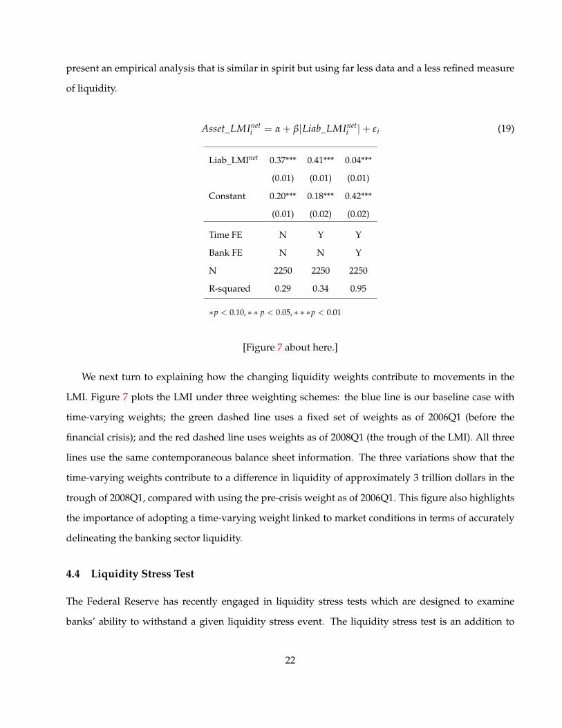
present an empirical analysis that is similar in spirit but using far less data and a less refined measure

of liquidity.

Asset_LMIneti = α + β|Liab_LMInet

i |+ ε i (19)

Liab_LMInet 0.37*** 0.41*** 0.04***

(0.01) (0.01) (0.01)

Constant 0.20*** 0.18*** 0.42***

(0.01) (0.02) (0.02)

Time FE N Y Y

Bank FE N N Y

N 2250 2250 2250

R-squared 0.29 0.34 0.95

∗p < 0.10, ∗ ∗ p < 0.05, ∗ ∗ ∗p < 0.01


We next turn to explaining how the changing liquidity weights contribute to movements in the

LMI. Figure 7 plots the LMI under three weighting schemes: the blue line is our baseline case with

time-varying weights; the green dashed line uses a fixed set of weights as of 2006Q1 (before the

financial crisis); and the red dashed line uses weights as of 2008Q1 (the trough of the LMI). All three

lines use the same contemporaneous balance sheet information. The three variations show that the

time-varying weights contribute to a difference in liquidity of approximately 3 trillion dollars in the

trough of 2008Q1, compared with using the pre-crisis weight as of 2006Q1. This figure also highlights

the importance of adopting a time-varying weight linked to market conditions in terms of accurately

delineating the banking sector liquidity.

4.4 Liquidity Stress Test

The Federal Reserve has recently engaged in liquidity stress tests which are designed to examine

banks’ ability to withstand a given liquidity stress event. The liquidity stress test is an addition to

22

the Supervisory Capital Assessment Program (SCAP), which has become a standard process to test

if a bank has sufficient capital to cover a given stress event. The decomposition of Figure 7 indicates

a simple methodology to run a liquidity stress test within our measurement framework. The only

difference across the three lines in Figure 7 are the liquidity weights, which in turn are determined

by the time-varying repo haircuts mt and the funding liquidity factor (µt). We suggest that a liquidity

stress test can be implemented as a set of realizations of the funding liquidity factor or repo haircut,

and these realizations can be traced through the liquidity weights to compute the stress effects on the

liquidity of a given bank.


We run a liquidity stress test at three time points: 2006Q1 (before the crisis), 2008Q1 (liquidity

trough) and 2012Q4 (Fed’s first liquidity stress test). Table 3 reports the results. Consider the first

column corresponding to 2008Q1. The first row in the benchmark, denoted as "T", corresponds to the

LMI value as of 2008Q1. The next line, denoted as "[0,T]”, reports the historical average LMI up to this

time point. We then compute the LMI under stress scenarios. The first line of the funding liquidity

scenario reports the LMI based on assets and liabilities as of 2008Q1, but using liquidity weights that

are based on one standard deviation (1-sigma) from the historical mean value of the funding liquidity

state variable. We similarly report numbers over the next few rows based on weights when funding

liquidity factor µt or haircut m̄t is 1, 2, and 6 sigmas away from historical mean values.

In 2006Q1, the aggregate liquidity mismatch was -2.09 trillion and its 2 sigma scenario under µ

predicts the liquidity condition as of 2008Q1, the most severe liquidity dry-up period.

5 LMI and the Cross-Section of Banks

The previous section presented one benchmark for evaluating the LMI, namely its utility from a

macro-prudential viewpoint. We now consider another benchmark for evaluating the LMI. If the LMI

contains information regarding the liquidity risk of a given bank, then changes in market liquidity

conditions will affect the stock returns of banks differentially depending on their LMI. That is, as

market liquidity conditions deteriorate, a firm with a worse liquidity position (lower LMI) should

23

experience a more negative stock return. Moreover, in the financial crisis, we would expect that firms

with a worse ex-ante LMI would depend more on liquidity support from the government.

We begin this section descriptively. We first show how the LMI of different banks varies over time,

and what characteristics of banks correlate with their LMI. We then examine the informativeness of

the LMI in a number of dimensions.

5.1 Cross-Sectional LMI

Figure 8 plots the cross-sectional distribution of the LMI over the universe of BHCs, with Panel A for

the LMI scaled by total assets and Panel B for the LMI in absolute dollar amount. The red solid line is

the median value while the shade area depicts the 10th to 90th percentiles.


The median value of the scaled LMI in Panel A follows the aggregate pattern in Figure 3. The

shaded region (10th and 90th percentiles) is also stable suggesting that bank holding companies tend

to have a stable cross-sectional distribution of liquidity. The version in Panel B, where LMI is not

scaled rather in dollar amount, tells a different story and indicates a vast heterogeneity across banks’

liquidity condition. The figure suggests that bank size (as measured by total assets) plays an important

role in differentiating the absolute amount of liquidity mismatch across banks. At the beginning of

the sample, the BHCs have a small dispersion in their liquidity conditions. The dispersion widens

noticeably after 2007, likely because of the development of structured financial products. After the

financial crisis, the dispersion narrowed again as some of these products are unwound, but remains

wider than in the early 2000s.

We plot the time-series LMI for twelve representative banks in Figure 9, with Panel A for LMI

scaled by total assets and Panel B for LMI in dollar amount. The LMI is negative for most of the

bank holding companies, illustrating the pervasive liquidity mismatch of the banking sector during

the crisis. For banks such as JPMorgan Chase, Bank of America, Wells Fargo, the LMI dramatically

deteriorated during the crisis, but improved steadily from 2009 onwards, yet remained negative

throughout the sample. For other banks like Goldman Sachs and Morgan Stanley, the LMI was also

24

negative but much smaller in magnitude.10 For banks like Citibank and Northern Trust, the LMI

was negative in the beginning but switched the sign after the crisis, indicating a liquidity-surplus

condition.


The absolute level of the LMI may be useful as an indicator of systemic importance (i.e. "SIFI"

status). For this purpose, we plot the bank-level LMI in dollar amount in Panel B, with the same y-

axis scale to allow comparison. In the cross-section, banks have strikingly different liquidity levels.

Banks like JP Morgan Chase, Bank of America, and Citigroup have large liquidity shortfall during the

crisis whereas banks like State Street Corp, Northern Trust have a far smaller liquidity shortfall.

We report the top 12 banks with the most significant liquidity mismatch in Table 4, based on

the average absolute LMI level over the whole sample. Banks with the most liquidity shortfall

also correspond with common notions of the "too-big-to-fail" banks: Bank of America, Citigroup, JP

Morgan Chase, Wachovia, and Wells Fargo taking the top positions. These banks experience their most

stressed liquidity conditions in 2008Q1. American Express (ranked tenth) had the largest liquidity

shortfall in the first quarter of 2009. The mortgage-related financial institution, Countrywide, saw it

biggest liquidity mismatch in 2006Q2, one year before the subprime crisis. We also report the top 5

banks with the best average liquidity condition. They are smaller banks, although still among the top

50 BHCs.

[Table 4 and 5 about here.]

We investigate the relationship between the LMI and bank characteristics for the universe of BHCs.

Table 5 shows the results of regressing scaled-LMI and absolute LMI (in dollar amount), on a set of

bank characteristics, which are collected from the Y-9C reports. The univariate specifications suggest

that banks tend to have lower scaled LMI (worse liquidity condition) when they have larger risk-

weighted assets, or more profitability (measured by return on asset (ROA)), or lower capital ratio.

The multivariate specification (4) shows that these results are robust after the inclusion of other BHC

10The data for Goldman Sachs and Morgan Stanley begin in 2009Q1 given that these investment banks converted to bankholding companies after the Lehman event in September 2008.

25

characteristics. Specifications (5)-(8) show the similar results using the absolute LMI as dependent

variable. Among all bank characteristics, risk-adjusted asset has the most explanatory power on bank

liquidity condition.

5.2 The Informativeness of LMI for Stock Market Performance

We first investigate the correlation between LMI and stock market performance.11 To this end, we

sort BHCs and construct two portfolios: LMI High and LMI Low, based on their scaled LMI values

averaged over the episode up to 2006Q1. Note that the unscaled LMI is driven almost entirely by

bank size, hence it is less suitable when we study the relationship between bank liquidity and stock

market performance (although as we have shown, the scaled LMI also correlates positively with size).

The High LMI portfolio contains 100 BHCs with the highest LMI (best liquidity condition), and the

Low LMI portfolio contains 100 BHCs with the lowest LMI (worst liquidity condition), in the universe

of public BHCs during the pre-crisis period. Table 6 describes the summary statistics of the banks

forming each of the two portfolios.

[Table 6 and Figure 10 about here.]

Figure 10 presents the cross-section of market performance, where equity market performance is

measured by the market capitalization of the portfolio normalized by its level as of 2006Q1. As shown

in the figure, the Low LMI portfolio of BHCs outperformed the High LMI portfolio before the crisis.

This pattern reversed in the crisis, when banks with a larger liquidity shortfall (the Low LMI portfolio)

experienced lower stock returns. The gap between Low and High portfolios continued widening till

2009Q1 (the episode when stock market tumbled to record low point), then narrowed down. The

pattern reversed again with the better performance of the Low LMI portfolio in the post-crisis period,

though the reverse lasts shortly.

One possible explanation for our finding is that hoarding liquidity is costly, and only generates

benefits in crises periods. Thus the low LMI banks are systematically more risky and more exposed

to crises than the high LMI banks. Berger and Bouwman (2009) show that banks which are the

11Given that the balance sheet information of foreign banks’ U.S. subsidiaries cannot match their parent companies’ stockmarket price, we exclude all foreign banks’ U.S. subsidiaries in this analysis.

26

most active in liquidity creation are rewarded by the stock market. We show that this correlation is

dramatically reversed in crisis times. This result provides support to the hypothesis that the banking

sector actively creates liquidity in good times (pre-crisis) but at the expense of building fragility, an

idea that is tested in the aggregate by Berger and Bouwman (2012). Our cross-sectional approach

identifies that the banks that create the most liquidity are the most vulnerable to financial crises.

5.3 The Informativeness of LMI for Bank Borrowing

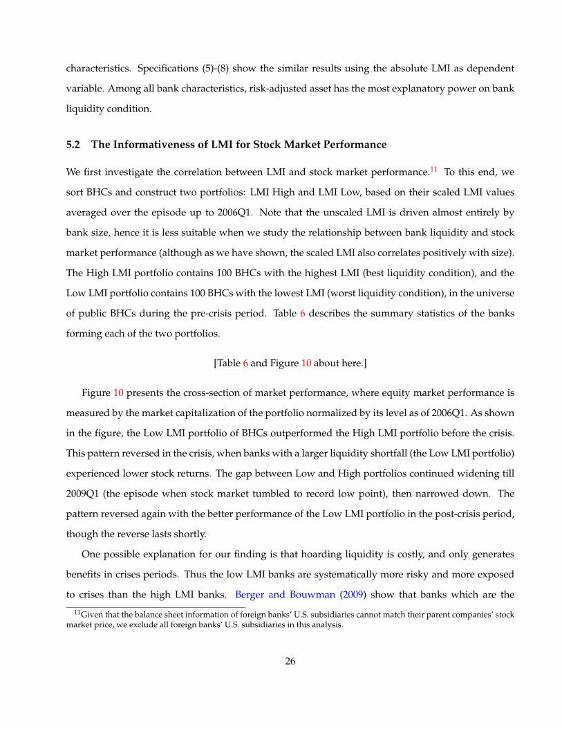
We ask whether banks with a worse liquidity condition rely more on the Federal Reserve and TARP

funding during the crisis. That is, is the LMI informative for the liquidity stress, and hence reliance

on government facilities, of a bank? Table 7 presents the results. The dependent variable in Panel A

is the log of loans from all Federal Reserve facilities (for details on these facilities see section 4.2). The

dependent variable in Panel B is of the log of funds from TARP. Independent variables are the log of

the absolute value of the LMI, calculated as of 2007Q2, 2008Q1, and 2006Q1. We also include controls

for other standard characteristics of banks, including capital and leverage, that may indicate a need to

borrow from the government. 12

The results indicate that the LMI is indeed informative regarding government borrowing, above

and beyond standard measures. The log-log specification indicates that a 1% increase in the LMI is

correlated with a between 0.51 and 0.86% increase in Fed borrowing. For TARP, the magnitudes range

from between 0.50% and 0.82%. We have also investigate a specification where the dependent variable

is a dummy indicating borrowing from the Fed. The results are broadly in line with those presented

in the table.


12Bayazitova and Shivdasani (2012) shows that strong banks opted out of receiving TARP money and equity infusionswere provided to banks that had high systemic risk, faced high financial distress costs, but had strong asset quality. Weprovide additional evidence by linking bank’s borrowing decision to their liquidity condition.

27

5.4 Event Study: LMI and Liquidity Shock

The LMI is intended to measure the the exposure of a bank to a liquidity stress event. If the LMI is

informative in this dimension then we should observe differential performance of banks with different

LMI across market-wide liquidity events. In particular, we expect that the banks with low LMI (poor

liquidity) to perform worse under a negative liquidity shock whereas it performs better under a

positive liquidity shock. We follow an event study methodology to test this hypothesis.

We sort the public BHCs and construct two portfolios according to their LMI values at the end of

previous quarter, LMI High and LMI Low. Each portfolio contains value-weighted 100 banks with the

highest/lowest LMI value. We use the Fama-French three-factor model to compute expected returns

within the estimation window of [t-180, t-30], where t denotes the event day of a liquidity shock.

We then choose significant liquidity events in the sample. These events are chosen based on

considering a large move in the TOIS spread as well as economic news such as the announcement

of Fed liquidity facilities. Note that events cluster in the crisis and hence obscure the effect of liquidity

shock. To identify a clean event, we choose the first event over any consecutive 30 days when the

TOIS makes a significant negative jump or when the Fed announces the creation of a liquidity-related

facility. We end-up with three events on positive liquidity shocks, PDCF (March 17, 2008), CPFF

(October 7, 2008), and TALF (November 25, 2008), as well as three events on negative liquidty shocks,

∆TOIS=-59bps (August 20, 2007), ∆TOIS=-30bps (October 10, 2008), and ∆TOIS=-53bps (September

17, 2008).


Figure 11 show the cumulative abnormal returns (CAR) during the [-2, 5] event window, with a

normalization on the event date t = 0. We observe that the Low LMI portfolio underperforms the

High LMI portfolio in days after a negative liquidity shock, whereas it overperforms the High LMI

portfolio after a positive liquidity shock, confirming our hypothesis.

28

6 Conclusion

This paper implements the liquidity measure, LMI, which evaluates the liquidity of a given bank

under a liquidity stress event that is parameterized by liquidity weights.

Relative to the Liquidity Coverage Ratio (LCR) of Basel III (which is conceptually closer to our

liquidity measurement exercise than the Net Stable Funding Ratio), the LMI has three principal

advantages. First, the LMI, unlike the LCR, can be aggregated across banks and thereby provide a

macro-prudential liquidity parameter. Second, the LCR uses an arbitrary liquidity horizon of 30 days.

Our implementation of the LMI links the liquidity horizon to market based measures of liquidity

premia as well as the aggregate LMI. Thus our measurement has the desirable feature that during a

financial crisis when liquidity premia are high, the LMI is computed under a longer-lasting liquidity

scenario. Likewise, when the aggregate LMI of the financial sector is high, indicating fragility of

the banking sector, the LMI is computed under a longer-lasting scenario. Third, the LMI framework

provides a natural methodology to implement liquidity stress tests.

The LMI has a close precedent, the Berger and Bouwman (2009) liquidity creation measure.

The primary change relative to the Berger-Bouwman measure is that the LMI is based on time-

and state-dependent liquidity weights. This is an important modification because it naturally links

bank liquidity positions to market liquidity conditions, and thus is better suited to serving as a

macroprudential barometer (and a stress testing framework). We have shown that the LMI performs

well relative to our macroprudential benchmarks. We have also shown that the LMI contains

important information regarding the liquidity risks in the cross-section of banks.

We do not view the LMI measures of this paper as a finished product. We have made choices

regarding the liquidity weights in computing the LMI. These weights play a central role in the

performance of the LMI against our macro and micro benchmarks. It will be interesting to bring

in further data to better pin down liquidity weights. Such data may be more detailed measures of

security or funding liquidity drawn from financial market measures. Alternatively, such data may be

balance sheet information from more banks, such as European banks, which will offer further data

on which to calibrate the LMI. In either case, the approach of this paper can serve as template for

developing a better liquidity measure.

29

References

Acharya, V., and O. Merrouche, 2013, “Precautionary Hoarding of Liquidity and Inter-Bank Markets:

Evidence from the Sub-prime Crisis,” Review of Finance, 17(1), 107–160.

Acharya, V., and N. Rosa, 2013, “A Crisis of Banks as Liquidity Providers,” Journal of Finance.

Acharya, V., and D. Skeie, 2011, “A Model of Liquidity Hoarding and Term Premia in Inter-Bank

Markets,” Journal of Monetary Economics, 58(5), 436–447.

Armantier, O., E. Ghysels, A. Sarkar, and J. Shrader, 2011, “Stigma in Financial Markets: Evidence

from Liquidity Auctions and Discount Window Borrowing during the Crisis,” Federal Reserve Bank

of New York Staff Reports, no. 483.

Banerjee, R. N., 2012, “Banking Sector Liquidity Mismatch and the Financial Crisis,” Bank of England

working paper.

Bayazitova, D., and A. Shivdasani, 2012, “Assessing TARP,” Review of Financial Studies, 25(2), 377–407.

Berger, A., and C. Bouwman, 2009, “Bank Liquidity Creation,” Review of Financial Studies, 22(9), 3779–

3837.

, 2012, “Bank Liquidity Creation, Monetary Policy, and Financial Crises,” working paper.

Berger, A., C. Bouwman, T. Kick, and K. Schaeck, 2013, “Bank Risk Taking and Liquidity Creation

following Regulatory Interventions and Capital Support,” working paper.

Brunnermeier, M. K., G. Gorton, and A. Krishnamurthy, 2011, “Risk Topography,” NBER

Macroeconomics Annual.

, 2012, “Liquidity Mismatch Measurement,” NBER Systemic Risk and Macro Modeling.

Copeland, A., A. Martin, and M. Walker, 2010, “The Tri-Party Repo Market before the 2010 Reforms,”

Federal Reserve Bank of New York Staff Report.

, 2011, “Repo Runs: Evidence from The Tri-Party Repo Market,” Federal Reserve Bank of New

York Staff Report.

30

de Haan, L., and J. W. v. d. End, 2012, “Bank liquidity, the maturity ladder, and regulation,” De

Nederlandsche Bank working paper.

Diamond, D., and P. Dybvig, 1983, “Bank Runs, Deposit Insurance, and Liquidity,” Journal of Political

Economy, 91, 401–419.

Ennis, H. M., and J. A. Weinberg, 2012, “Over-the-counter Loans, Adverse Selection, and Stigma in the

Interbank Market,” Review of Economic Dynamics.

Fleming, M., 2012, “Federal Reserve Liquidity Provision during the Financial Crisis of 2007-2009,”

Annual Review of Financial Economics, 4, 161–177.

Furfine, C. H., 2003, “Standing facilities and interbank borrowing: Evidence from the federal reserve’s

new discount window,” International Finance, 6, 329–347.

Gorton, G., and A. Metrick, 2012, “Securitized Banking and the Run on Repo,” Journal of Financial

Economics, 104(3), 425–451.

Gorton, G., and G. Pennacchi, 1990, “Financial Intermediaries and Liquidity Creation,” Journal of

Finance, 45(1), 49–71.

Hanson, S. G., A. Shleifer, J. C. Stein, and R. W. Vishny, 2014, “Banks as Patient Fixed Income

Investors,” Federal Reserve Board working paper.

He, Z., I. G. Khang, and A. Krishnamurthy, 2010, “Balance Sheet Adjustment in the 2008 Crisis,” IMF

Economic Review, 1, 118–156.

Heider, F., M. Hoerova, and C. Holhausen, 2009, “Liquidity Hoarding and Interbank Market Spreads:

The Role of Counterparty Risk,” European Central Bank working paper No. 1126.

Holmstrom, B., and J. Tirole, 1998, “Private and public supply of liquidity,” Journal of Political Economy,

106(1), 1–40.

Krishnamurthy, A., S. Nagel, and D. Orlov, 2014, “Sizing Up Repo,” Journal of Finance.

31

Krishnamurthy, A., and A. Vissing-Jorgensen, 2013, “The Ins and Outs of Large Scale Asset

Purchases,” Kansas City Federal Reserve Symposium on Global Dimensions of Unconventional Monetary

Policy.

Nagel, S., 2014, “The Liquidity Premium of Near-Money Assets,” Working paper, University of Michigan.

Peristiani, S., 1998, “The growing reluctance to borrow at the discount window: An empirical

investigation,” Review of Economics and Statistics, 80, 611 – 620.

Rochet, J.-C., and X. Vives, 2004, “Coordination Failures and the Lender of Last Resort: Was Bagehot

Right After All?,” Journal of the European Economic Association.

Smith, J., 2012, “The Term Structure of Money Market Spreads During the Financial Crisis,” mimeo.

Stein, J. C., 2013, “Liquidity Regulation and Central Banking,” Speech at the "Finding the Right Balance"

2013 Credit Markets Symposium sponsored by the Federal Reserve Bank of Richmond, Charlotte, North

Carolina.

Taliaferro, R., 2009, “"Where Did the Money Go?" Commitments, Troubled Assets, New Lending, and

the Capital Purchase Program,” Harvard Business School working paper.

32

Table 1: Summary Statistics of Bank Holding Companies in Y9-C Reports during 2006-2013

Panel A

Universe (N=1507) Public (N=509) Public US (N=481) TOP 50 US

mean std mean std mean std mean std

Total Asset ($Mil) 14.89 120.84 35.30 204.39 34.13 205.30 360.85 619.11

Leverage 0.91 0.04 0.91 0.03 0.91 0.03 0.90 0.02

Foreign/Total Deposit 0.01 0.05 0.01 0.07 0.01 0.07 0.11 0.21

Risk-adj. Asset ($Mil) 9.60 74.83 22.65 126.90 22.30 127.90 233.65 380.80

Tier1 Capital Ratio 12.59 5.66 12.30 4.01 12.35 3.96 11.19 2.63

Total Capital Ratio 14.20 5.56 13.89 3.84 13.93 3.79 14.04 2.54

Tier1 Leverage Ratio 9.24 3.50 9.21 2.47 9.26 2.42 8.50 1.94

ROA (annualized) 1.24 4.30 0.96 3.93 0.97 3.95 1.42 3.36

ROE (annualized) 18.57 49.95 16.26 44.89 16.41 45.18 19.71 33.31

Panel B: Top 50 BHCs (rank is based on total asset values as of 2006:Q1)

Tier1 Tier1 Risk-based

Rank Company Size($Bil) Leverage Lev. Ratio Capital Ratio

1 CITIGROUP 1884.32 0.93 5.16 8.59

2 BANK OF AMER CORP 1463.69 0.91 6.36 8.64

3 JPMORGAN CHASE 1351.52 0.91 6.19 8.66

4 WACHOVIA CORP 707.12 0.90 6.01 7.42

5 METLIFE 527.72 0.93 5.55 9.51

6 WELLS FARGO 482.00 0.90 7.89 8.95

7 HSBC NORTH AMER HOLD 478.16 0.93 5.90 8.13

8 TAUNUS CORP 430.40 0.99 -0.82 -3.97

9 BARCLAYS GROUP US 261.22 0.99 1.08 10.96

10 US BC 219.23 0.90 8.16 8.75

20 BANK OF NY CO 103.46 0.89 6.67 8.19

30 UNIONBANCAL CORP 52.62 0.91 8.44 8.68

40 SYNOVUS FC 31.89 0.88 10.64 10.87

50 WEBSTER FNCL CORP 17.10 0.89 7.68 9.21

Total 10581.94 0.92 6.07 8.04

33

Table 2: Haircuts by Collateral type

Collateral Mean Std P5 P25 P50 P75 P95

Treasuries .023 .021 .020 .020 .020 .020 .029

Agencies .026 .030 .020 .020 .020 .029 .033

CommPaper .029 .010 .020 .020 .029 .033 .048

Municipals .039 .021 .020 .020 .038 .048 .091

StrucFinance .046 .036 .020 .020 .032 .071 .091

CorporateDebt .048 .033 .020 .029 .048 .056 .085

ForeignDebt .055 .036 .021 .030 .048 .053 .106

Equities .063 .020 .048 .048 .048 .077 .094

Average .030 .030 .020 .020 .020 .029 .074

34

T=20

08Q

1T=

2006

Q1

T=20

12Q

4

LMI

LMI

LMI

Benc

hmar

kBe

nchm

ark

Benc

hmar

k

T-3

.26

T-2

.09

T-0

.65

[0,T

]-1

.80

[0,T

]-1

.38

[0,T

]-1

.55

Stre

ssSc

enar

ios

Stre

ssSc

enar

ios

Stre

ssSc

enar

ios

µ[0

,T]−

σ[0

,T]

-4.0

3µ[0

,T]−

σ[0

,T]

-2.6

2µ[0

,T]−

σ[0

,T]

-1.3

0

µµ[0

,T]−

2σ[0

,T]

-4.9

1µ

µ[0

,T]−

2σ[0

,T]

-3.2

2µ

µ[0

,T]−

2σ[0

,T]

-2.0

5

µ[0

,T]−

6σ[0

,T]

-6.5

8µ[0

,T]−

6σ[0

,T]

-5.2

2µ[0

,T]−

6σ[0

,T]

-5.9

2

µ[0

,T]+

σ[0

,T]

-3.3

1µ[0

,T]+

σ[0

,T]

-2.1

4µ[0

,T]+

σ[0

,T]

-0.6

7

m̄µ[0

,T]+

2σ[0

,T]

-3.3

6m̄

µ[0

,T]+

2σ[0

,T]

-2.1

8m̄

µ[0

,T]+

2σ[0

,T]

-0.7

5

µ[0

,T]+

6σ[0

,T]

-3.5

6µ[0

,T]+

6σ[0

,T]

-2.3

5µ[0

,T]+

6σ[0

,T]

-1.0

3

Tabl

e3:

Liqu

idit

ySt

ress

Test

usin

gLM

I.Th

eta

ble

repo

rts

the

aggr

egat

eLM

I(i

n$t

rilli

on)

over

allB

HC

sun

der

stre

sssc

enar

ios

whe

nth

efu

ndlin

gliq

uidi

tyfa

ctor

orth

ecr

oss-

colla

tera

lave

rage

hair

cutd

evia

te1-

,2-,

6-σ

away

from

the

hist

oric

alm

ean

upto

each

tim

epo

intT

.All

tim

e-se

ries

star

ton

2002

q1.

35

Table 4: Banks with the most Significant Liquidity MismatchThis table shows the LMI summary statistics for selected banks. Panel A presents the summary for banks with the mostnegative LMI in dollar amount out of the Top 50 banks, ranked by the average LMI values across the sample of 2006Q1 to2012Q1; Panel B presents the results for banks with the most positive dollar LMI out of the Top 50 banks, that is, with thebest liquidity condition. BHC with only one quarterly observation are excluded from the list. Time indicates the quarter atwhich the absolute LMI is the lowest for a given BHC.

Panel A: Banks with the most negative dollar LMI (mean)

LMI (in $bil)Name Net LMI Mean Median Std Min Time

1. JPMorgan Chase -0.22 -235 -186 142 -541 2008Q3

2. Bank of America -0.15 -229 -209 130 -505 2008Q1

3. Citigroup -0.10 -147 -175 209 -565 2008Q1

4. Wachovia -0.14 -78 -82 40 -165 2007Q4

5. Wells Fargo -0.12 -74 -74 37 -217 2008Q4

6. Morgan Stanley -0.10 -66 -66 12 -91 2013Q1

7. Goldman Sachs -0.07 -53 -50 16 -78 2012Q4

8. US BC -0.15 -38 -41 15 -63 2008Q1

9. Bank of NY -0.32 -32 -30 17 -55 2006Q4

10. American Express -0.22 -32 -30 6 -42 2012Q2

11. Countrywide -0.23 -29 -28 14 -48 2005Q4

12. Capital One -0.19 -27 -26 13 -51 2007Q4

Panel B: Banks with the most positive dollar LMI (mean)

LMI (in $bil)Name Net LMI Mean Median Std Min Time

1. E Trade 0.13 7 6 1 5 2013Q1

2. IMB 0.19 5 5 0 5 2012Q1

3. Northern Trust 0.03 5 -1 13 -12 2007Q2

4. Commerce 0.06 1 1 2 -4 2007Q4

5. First Niagara 0.00 0 0 1 -1 2011Q3

36

Table 5: The Relationship of LMI with Bank CharacteristicsThis table presents the results of pooled cross-sectional regression for the universe of public bank holding companies during2006Q1 to 2012Q1. The standard errors are robust and clustered by bank. All variables are adimensional (ratios) except TotalAssets, Risk-adjusted Assets and Unscaled LMI are in billion dollars.

Depend variable: Scaled LMI Depend variable: Unscaled LMI

(1) (2) (3) (4) (5) (6) (7) (8)

Risk-adj. Assets -0.19*** -0.14 -0.29*** -0.48

(0.06) (0.60) (0.04) (0.58)

Tier1 Capital Ratio 1.36*** 1.81* 0.14** -0.45

(0.35) (0.93) (0.06) (0.33)

ROA (annualized) -0.53*** -0.60*** -0.04** -0.02*

(0.11) (0.12) (0.02) (0.01)

Total Assets -0.03 0.12

(0.41) (0.37)

Total Capital Ratio 0.88 0.46

(0.87) (0.33)

Tier1 Leverage Ratio -2.54*** 0.16*

(0.70) (0.10)

ROE (annualized) -0.02** -0.00

(0.01) (0.00)

Constant -0.08*** -0.25*** -0.08*** -0.18*** -0.00 -0.02** -0.01** -0.02

(0.01) (0.04) (0.01) (0.05) (0.00) (0.01) (0.00) (0.02)

N 6055 6055 6057 6055 6055 6055 6057 6055

R-squared 0.02 0.11 0.02 0.22 0.53 0.01 0.00 0.54

* p<0.10, ** p<0.05, *** p<0.01

37

Tabl

e6:

Cha

ract

eris

tics

ofLM

IHig

h/Lo

wPo

rtfo

lios

This

tabl

etr

acks

the

bank

char

acte

rist

ics

oftw

opo

rtfo

lios,

LMIH

igh

and

LMIL

ow,i

nth

epr

e-cr

isis

,the

cris

is,a

ndth

epo

st-c

risi

spe

riod

.All

publ

icBH

Cs

are

sort

edba

sed

onth

eir

scal

edLM

Ival

ues

aver

aged

over

the

pre-

cris

isep

isod

e(2

006Q

1-20

07Q

2).T

heLM

IHig

hpo

rtfo

lioco

ntai

ns10

0BH

Cs

wit

hth

ehi

ghes

tLM

I(be

stliq

uidi

tyco

ndit

ion)

,and

the

LMIL

owpo

rtfo

lioco

ntai

ns10

0BH

Cs

wit

hth

elo

wes

tLM

I(w

orst

liqui

dity

cond

itio

n).

All

Publ

icU

SBH

Cs

(Top

100/

Bott

om10

0)

Pre-

Cri

sis

(200

6Q1:

2007

Q2)

Cri

sis

(200

7Q3:

2009

Q2)

Post

-Cri

sis

(200

9Q3:

2012

Q1)

Low

Hig

hLo

wH

igh

Low

Hig

h

mea

nst

dm

ean

std

mea

nst

dm

ean

std

mea

nst

dm

ean

std

Tota

lAss

et($

Mil)

46.3

617

5.69

2.14

6.00

58.4

224

0.65

2.64

8.15

74.2

630

9.68

3.27

10.0

9

Leve

rage

0.91

0.03

0.90

0.03

0.91

0.04

0.90

0.03

0.90

0.04

0.90

0.03

Fore

ign/

Tota

lDep

osit

0.01

0.04

0.01

0.07

0.01

0.03

0.01

0.07

0.01

0.02

0.01

0.06

Ris

k-ad

j.A

sset

($M

il)35

.32

127.

491.

453.

9944

.90

177.

931.

805.

3851

.20

206.

422.

056.

09

Tier

1C

apR

atio

10.6

02.

7414

.16

4.70

10.5

94.

3613

.11

3.52

12.7

74.

3814

.20

3.81

Tota

lCap

Rat

io12

.41

2.45

15.3

74.

5712

.51

4.13

14.3

63.

4114

.82

4.16

15.6

23.

71

Tier

1Le

vera

ge8.

971.

789.

792.

269.

012.

809.

612.

409.

603.

099.

452.

17

RO

A(a

nnua

lized

)2.

411.

702.

041.

76-0

.29

6.33

1.48

3.04

-0.5

54.

550.

963.

75

RO

E(a

nnua

lized

)31

.12

23.7

624

.81

22.8

28.

7248

.58

19.3

731

.20

0.73

55.5

814

.26

42.7

5

38

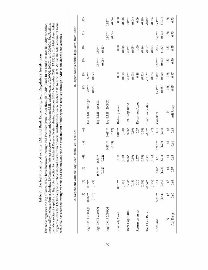
Tabl

e7:

The

Rel

atio

nshi

pof

exan

teLM

Iand

Bank

Borr

owin

gfr

omR

egul

ator

yIn

stit

utio

nsTh

ista

ble

regr

esse

sth

elo

gof

loan

sBH

Cs

have

borr

owed

thro

ugh

Fed

Faci

litie

s(P

anel

A)o

rth

roug

hTA

RP

(Pan

elB)

onba

nks’

exan

teliq

uidi

tyco

ndit

ion,

mea

sure

dby

the

loga

rith

mof

abso

lute

LMIa

mou

nt.W

ete

stth

ree

exan

tesc

enar

ios,

that

are

LMIs

calc

ulat

edas

of20

07Q

2,20

08Q

1,an

d20

06Q

1.Fe

dFa

cilit

ies

incl

ude

ase

ries

ofca

pita

land

liqui

dity

inje

ctio

nby

the

Fede

ralR

eser

veSy

stem

duri

ngD

ecem

ber

2007

-N

ovem

ber

2008

.TA

RP,

the

Trou

bled

Ass

etR

elie

fPr

ogra

mal

low

sth

eU

STr

easu

ryto

purc

hase

illiq

uid

asse

tsfr

omfin

anci

alin

stit

utio

nsbe

twee

nO

ctob

er20

08to

June

2009

.W

eus

eth

eto

tala

mou

ntof

loan

sea

chBH

Cha

sac

cess

edth

roug

hva

riou

sFe

dFa

cilit

ies,

and

use

the

tota

lam

ount

ofm

oney

bank

sre

ceiv

edth

roug

hTA

RP

asth

ede

pend

entv

aria

bles

.

A.D

epen

dant

vari

able

:log

(Loa

n)fr

omFe

dFa

cilit

ies

B.D

epen

dant

vari

able

:log

(Loa

n)fr

omTA

RP

(1)

(2)

(3)

(4)

(5)

(6)

(7)

(8)

(9)

(10)

(11)

(12)

log|

LMI|

2007

Q2

0.86

***

0.59

**lo

g|LM

I|20

07Q

20.

70**

*0.

66**

*

(0.1

0)(0

.21)

(0.0

5)(0

.07)

log|

LMI|

2006

Q1

0.74

***

0.51

**lo

g|LM

I|20

06Q

10.

57**

*0.

50**

*

(0.1

2)(0

.22)

(0.0

8)(0

.13)

log|

LMI|

2008

Q1

0.83

***

0.61

***

log|

LMI|

2008

Q1

0.80

***

0.82

***

(0.0

9)(0

.12)

(0.0

4)(0

.06)

Ris

k-ad

jAss

et0.

01**

*0.

000.

01**

*R

isk-

adjA

sset

0.00

0.00

0.00

(0.0

0)(0

.00)

(0.0

0)(0

.00)

(0.0

0)(0

.00)

Tier

1C

apR

atio

0.33

*0.

36*

0.36

*Ti

er1

Cap

Rat

io0.

11**

*0.

12**

*0.

08**

(0.1

8)(0

.19)

(0.1

9)(0

.03)

(0.0

5)(0

.04)

Ret

urn

onA

sset

0.10

1.57

*0.

07R

etur

non

Ass

et0.

481.

000.

09

(0.0

8)(0

.78)

(0.2

8)(0

.31)

(0.8

6)(0

.18)

Tier

1Le

vR

atio

-0.6

4**

-0.4

7-0

.52*

Tier

1Le

vR

atio

-0.1

0**

-0.1

2*-0

.06*

(0.2

9)(0

.36)

(0.2

7)(0

.05)

(0.0

7)(0

.03)

Con

stan

t-5

.24*

**0.

41-3

.16*

-1.8

1-4

.90*

**-1

.31

Con

stan

t-4

.74*

**-4

.88*

-2.8

7***

-2.6

3-6

.20*

**-6

.74*

**

(1.4

4)(4

.90)

(1.7

3)(5

.71)

(1.2

7)(2

.01)

(0.6

5)(0

.90)

(0.9

3)(1

.67)

(0.9

3)(1

.01)

N67

6764

6468

68N

168

168

153

153

176

176

Adj

R-s

qr0.

600.

630.

570.

650.

610.

63A

djR

-sqr

0.65

0.67

0.50

0.55

0.73

0.73

39

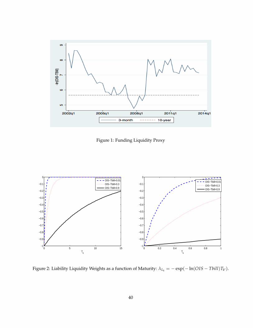
Figure 1: Funding Liquidity Proxy

0 5 10 15−1

−0.9

−0.8

−0.7

−0.6

−0.5

−0.4

−0.3

−0.2

−0.1

0

Tk

OIS−Tbill=0.01OIS−Tbill=0.3OIS−Tbill=0.9

0 0.2 0.4 0.6 0.8 1−1

−0.9

−0.8

−0.7

−0.6

−0.5

−0.4

−0.3

−0.2

−0.1

0

Tk

OIS−Tbill=0.01OIS−Tbill=0.3OIS−Tbill=0.9

Figure 2: Liability Liquidity Weights as a function of Maturity: λLk = − exp(− ln(OIS− Tbill)Tk′).

40

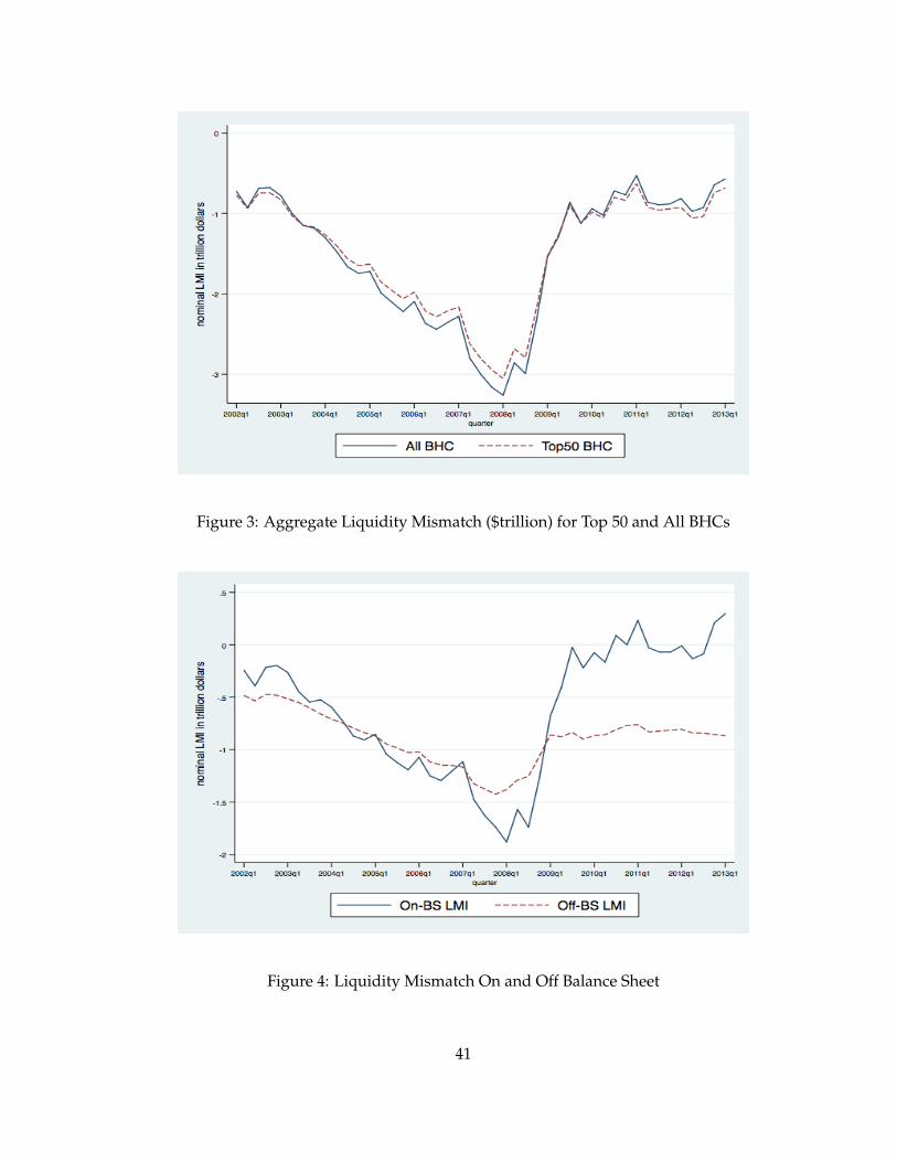
Figure 3: Aggregate Liquidity Mismatch ($trillion) for Top 50 and All BHCs

Figure 4: Liquidity Mismatch On and Off Balance Sheet

41

A: LMI post-crisis minus LMI in the crisis

B: LMI post-crisis minus LMI pre-crisis

Figure 5: Correlation between Fed Injections and the Change of LMI (in dollar amount)

42

A. Asset-side Liquidity (∑ λt,Ak xit,Ak

) B. Liability-side Liquidity (∑ λt,Lk′ xit,Lk′

)

C. Distribution of the Asset/Liability Liquidity Ratio (∑ λt,Ak xit,Ak

/|∑ λt,Lk′ xit,Lk′

|)

Figure 6: Decomposition of LMI by Assets and Liabilities for Top 50 BHCs. The red solid line is themedian value while the shade area depicts the 10th to 90th percentile.

43

Figure 7: LMI under various Liquidity Weights

44

A: LMI Scaled by Total Asset

B: LMI in Absolute Dollar Amount ($Billion)

Figure 8: Cross-sectional Distribution of Scaled and Dollar LMI for All BHCs. The red solid line is themedian value and the shade area depicts the 10th to 90th percentile. The sample is the universe ofBHCs filling Y-9C reports.

45

Panel A: LMI scaled by Total Assets

Figure 9: Selected Bank-Level Liquidity Mismatch

46

Panel B: LMI in dollar amount ($Thousand)

Figure 9 (Cont’d) Selected Bank-Level Liquidity Mismatch

47

Figure 10: Equity Market Capitalization by ex ante LMI Portfolios. The figure shows the marketcapitalization scaled by the level as of 2006Q1 for the Low (bottom 100 banks) and High (top 100banks) portfolios sorted by the average LMI during the pre-crisis period: 2006Q1 - 2007Q2, across allpublic BHCs. For consistency of balance sheet information and stock market performance, we excludethe U.S. subsidiaries of foreign banks.

48

Negative Shock Positive Shock

Figure 11: Event Study: LMI and Liquidity Shock. The figure shows the cummulative abnormal returnfor LMI low (bottom 100 banks) and LMI high (top 100 banks) portfolios sorted by the LMI at the endof previour quarter before an event. Negative events are selected based on the daily change of Tbill-OIS spread, and positive events are selected based on the announcement of Federal Reserve Liquidityfacilities.

49

Appendix

A Computing the LMI

We propose an integrated measure of the Liquidity Mismatch undertaken by individual banks. We

factor in all the balance sheet information and account for the effect of each balance sheet entry on

the liquidity pressure faced by a bank. The implementation of the LMI is parsimonious yet captures

the key degrees of liquidity variability (balance-sheet item heterogeneity and time-series variation).

Moreover, the methodology developed in this paper is flexible and can be improved on in future

research. For instance, the βL′ksensitivity parameters can be refined and could be estimated, for

example, by regressing the corresponding-maturity bond yield on the funding liquidity factor.

ASSETS

Category Ak λAk

Cash cash and balances due from depository institutions 1

federal funds sold 1

securities purchased under agreements to resell 1

Trading Assets Treasury securities (1−mTrsy)

agency securities, excluding MBS (1−mAgency)

residential MBS guaranteed by FNMA, FHLMC, or GNMA (1−mAgency)

securities Issued by States and U.S. Pol. Subdivisions (1−mMuni)

non-agency MBS (1−mStrucFin)

structured product (1−mStrucFin)

corporate debt (1−mCorporateDebt)

Available for Sale Treasury securities 0.75(1−mTrsy)

agency securities, excluding MBS 0.75(1−mAgency)

residential MBS guaranteed by FNMA, FHLMC, or GNMA 0.75(1−mAgency)

securities Issued by States and U.S. Pol. Subdivisions 0.75(1−mMuni)

50

non-agency MBS 0.75(1−mStrucFin)

structured product 0.75(1−mStrucFin)

corporate debt 0.75(1−mCorporateDebt)

foreign debt 0.75(1−mForeignDebt)

equity securities 0.75(1−mEquity)

Held for Maturity Treasury securities 0.50(1−mTrsy)

agency securities, excluding MBS 0.50(1−mAgency)

residential MBS guaranteed by FNMA, FHLMC, or GNMA 0.50(1−mAgency)

securities Issued by States and U.S. Pol. Subdivisions 0.50(1−mMuni)

non-agency MBS 0.50(1−mStrucFin)

structured product 0.50(1−mStrucFin)

corporate debt 0.50(1−mCorporateDebt)

foreign debt 0.50(1−mForeignDebt)

Loans loans secured by real estates 0.25(1−mStrucFin)

commercial & Industry Loans 0.50(1−Max{mk})

other Loans 0.50(1−Max{mk})

lease financing receivables 0.50(1−Max{mk})

Fixed Assets premises and fixed assets 0

other real estate owned 0

investment in unconsolidated subsidiaries 0

Intangible Assets goodwill and other intangible assets 0

Other Assets 0

LIABILITIES: λL = − exp(−µTk′)

Category Lk′ Tk′

51

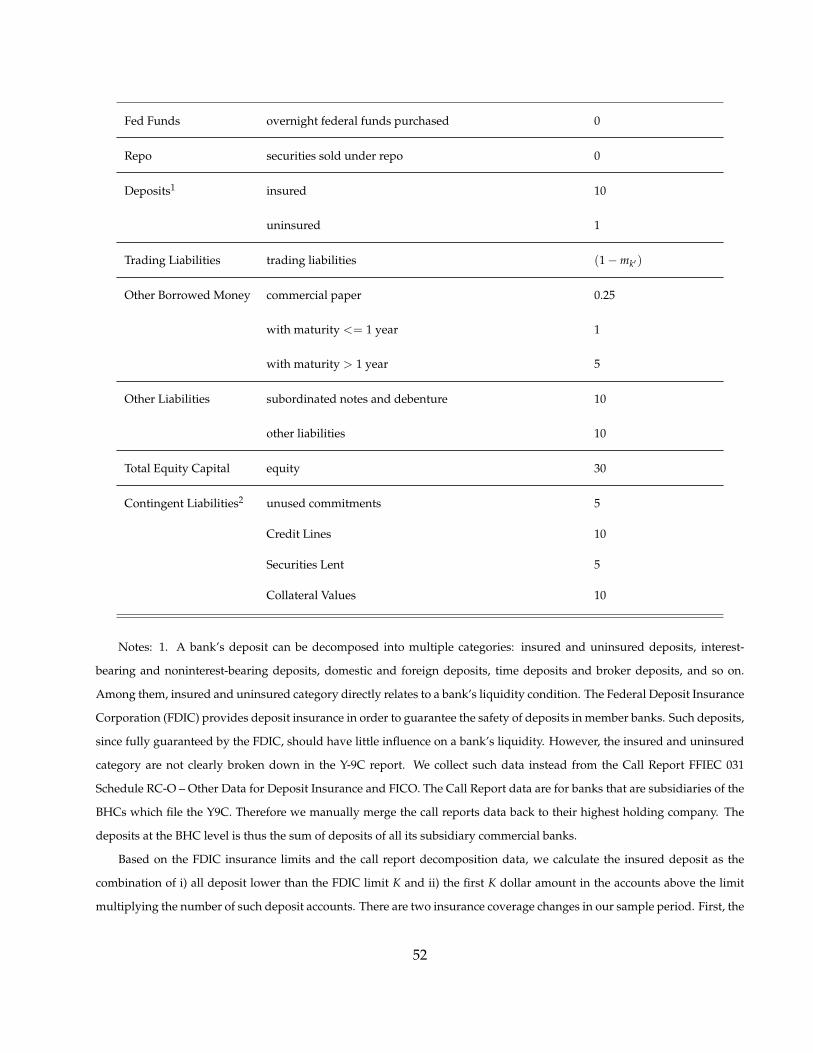
Fed Funds overnight federal funds purchased 0

Repo securities sold under repo 0

Deposits1 insured 10

uninsured 1

Trading Liabilities trading liabilities (1−mk′ )

Other Borrowed Money commercial paper 0.25

with maturity <= 1 year 1

with maturity > 1 year 5

Other Liabilities subordinated notes and debenture 10

other liabilities 10

Total Equity Capital equity 30

Contingent Liabilities2 unused commitments 5

Credit Lines 10

Securities Lent 5

Collateral Values 10

Notes: 1. A bank’s deposit can be decomposed into multiple categories: insured and uninsured deposits, interest-

bearing and noninterest-bearing deposits, domestic and foreign deposits, time deposits and broker deposits, and so on.

Among them, insured and uninsured category directly relates to a bank’s liquidity condition. The Federal Deposit Insurance

Corporation (FDIC) provides deposit insurance in order to guarantee the safety of deposits in member banks. Such deposits,

since fully guaranteed by the FDIC, should have little influence on a bank’s liquidity. However, the insured and uninsured

category are not clearly broken down in the Y-9C report. We collect such data instead from the Call Report FFIEC 031

Schedule RC-O – Other Data for Deposit Insurance and FICO. The Call Report data are for banks that are subsidiaries of the

BHCs which file the Y9C. Therefore we manually merge the call reports data back to their highest holding company. The

deposits at the BHC level is thus the sum of deposits of all its subsidiary commercial banks.

Based on the FDIC insurance limits and the call report decomposition data, we calculate the insured deposit as the

combination of i) all deposit lower than the FDIC limit K and ii) the first K dollar amount in the accounts above the limit

multiplying the number of such deposit accounts. There are two insurance coverage changes in our sample period. First, the

52

FDIC increased insurance limits from $100,000 to $250,000 per depositor on October 3, 2008. Yet this change is not reflected

in the Call Report RC-O until 2009:Q3. We follow the data availability and change our definition for insured/uninsured

deposit beginning in 2009:Q3. Second, the FDIC increased the insurance for retirement accounts from $100,000 to $250,000

on March 14, 2006. This change is reflected in the 2006:Q2 call reports and our definition reflects this change beginning in

2006:Q2.

2. We study four types of contingent liabilities that may exert a pressure on bank’s liquidity. Many banks carry unused

commitments, including revolving loans secured by residential properties, unused credit card lines, commitments to fund

commercial real estate, construction, and land development loans, securities underwriting, commitments to commercial and

industrial loans, and commitments to provide liquidity to asset-backed commercial paper conduits and other securitization

structures. The second type are credit lines, including financial standby letters of credit and foreign office guarantees,

performance standby letters of credit and foreign office guarantees, commercial and similar letters of credit.13 A third

type of contingent liability is securities lent. The last type of contingent liability in our study is the derivative contract.

Item 7 in Schedule HC-L lists the gross notional amount of credit derivative contracts, including credit default swaps,

total return swaps, credit options and other credit derivatives. However, such gross notional amount does not reflect the

contracts’ liquidity. What matters in a credit derivative contract in terms of liquidity impact is the additional collateral or

margin required in a stress event. We therefore use Item 15 to collect the fair value of collateral posted for over-the-counter

derivatives.14

B Background on Federal Liquidity Injection

The Federal Reserve System (Fed) undertook numerous measures to restore economic stability from the financial crisis of

2007 - 2009. Beyond its conventional monetary policy tools, the central bank, citing "unusual and exigent circumstances,"

launched a range of new programs to the banking sector in order to support overall market liquidity.

Conventionally, the Fed uses open market operations and the discount window as its principal tools to manage reserves

in the banking sector. During the crisis, however, the effectiveness of the discount window was limited because of a sigma

effect. Banks were reluctant to approach the discount window since such action could cause market participants to draw

13Berger and Bouwman (2009) consider unused commitments and standby letters of credit as asset-side liquidity whereaswe treat them as liability-side liquidity. It’s true that unused commitments and credit lines are similar to loans and hencecan be treated as assets, yet they become assets only when used. In terms of liquidity, they belong to potential liquidityoutflow as other liability classes. Therefore we treat them in line with liabilities given the common feature that they all exertliquidity pressure.

14The collateral type contains U.S. Treasury securities, U.S. government and government-sponsored agency debtsecurities, corporate bonds, equity securities, and other collateral. The collateral value is further divided into groups bythe counterparty, for example, a) bank and security firms, b) Monoline financial guarantors, c) hedge funds, d) sovereigngovernments, and e) corporations and all other counterparties.

Data under item 15 is required to be completed only by the bank holding companies with total assets of 10$billion ormore, and such requirement starts only since the second quarter of 2009. Not surprisingly, we only find such data for largeBHCs such as J.P. Morgan Chase, Bank of America, etc.

53

adverse inference about the bank’s financial condition (see, for example, Peristiani (1998), Furfine (2003), Armantier, Ghysels,

Sarkar, and Shrader (2011)).

Given the borrowing stigma and inflexibility of open market operations, the Fed proceeded to introduce additional

facilities increase liquidity, including the Term Auction Facility (TAF), Term Securities Lending Facility (TSLF), Primary

Dealer Credit Facility (PDCF), Asset-Backed Commercial Paper Money Market Mutual Fund Liquidity Facility (AMLF),

Commercial Paper Funding Facility (CPFF), Money Market Investor Funding Facility (MMIFF), and Term Asset-Backed

Securities (TALF). Fleming (2012) provides a summary on these lending facilities. We summarize their key features in the

following table.

Facility Announcement Expiration Participants Term

TAF Dec12, 2007 Mar08, 2010 Depository Inst. 28 or 84 days

TSLF Mar11, 2008 Feb01, 2010 Primary dealers 28 days

PDCF Mar17, 2008 Feb01, 2010 Primary dealers overnight

AMLF Sep19, 2008 Feb01, 2010 BHCs and branches <120 days for D∗

of foreign banks <270 days for non-D

CPFF Oct07, 2008 Feb01, 2010 U.S. CP issuers 3 months

MMIFF Oct21, 2008 Oct30, 2009 Money Mkt Funds 90 days or less

TALF Nov25, 2008 Jun30, 2010 U.S. eligible banks <5 years

*: D denotes depository institutions; non-D is non-depository institutions.

The Fed announced the first facility, Term Auction Facility (TAF) on December 12, 2007 to address the funding pressure

in short-term lending markets. Through the TAF, the Fed auctioned loans to depository institutions, typically for terms of

28 or 84 days. Later, to address liquidity pressures in the term funding markets, the Feds introduced the Term Securities

Lending Facility (TSLF) on March 11, 2008. Through TSLF, the Fed auctioned loans of Treasury securities to primary dealers

for terms of 28 days. Another related facility, the Primary Dealer Credit Facility (PDCF), was announced on March 16,

through which the Fed made overnight loans to primary dealers. The bankruptcy of Lehman Brothers on September

15, 2008 led to unparalleled disruptions of the money market. On September 19, the Fed announced created the Asset-

Backed Commercial Paper Money Market Mutual Fund Liquidity Facility (AMLF). It provided loans to U.S. bank holding

companies, and U.S. branches and agencies of foreign banks to purchase eligible asset-backed commercial paper from money

market mutual funds. On October 7, the Fed further announced the creation of the Commercial Paper Funding Facility

(CPFF), through which the Fed provided credit to a special-purpose vehicle (SPV) that, in turn, bought newly issued three-

month commercial paper. Two weeks later on October 21, the Fed established the Money Market Investor Funding Facility

(MMIFF). All three money market-related facilities expired on February 1, 2010. Lastly, the Fed introduced the Term Asset-

Backed Securities (TALF) on November 25, 2008, through which the Fed made loans to borrowers with eligible asset-backed

securities as collateral.

54

Measuring Liquidity Mismatch in the Banking Sector · PDF fileMeasuring Liquidity Mismatch in...

Documents

Transcript of Measuring Liquidity Mismatch in the Banking Sector · PDF fileMeasuring Liquidity Mismatch in...