Measuring financial risk

Sebastiano Manzan

ECO 4051 | Spring 2017

1 / 60

Why measure and manage risk?

I The risk-return tradeoff is at the core of any business and financial decision

I Modern companies and financial institutions are large enterprises with many(thousands?) of individuals making decisions in an uncertain environment

I How can we measure, aggregate, and manage (= control) the overall riskexposure of an organization?

I What type of risks are we trying to measure and control?

2 / 60

Types of financial risk

I Market risk: losses due to movements in the level and/or volatility of assetprices

I directional: exposure to movements of the marketI non-directional: exposure to changes of volatility

I Credit risk: losses arising from defaults on bonds and loans; changes tocredit ratings or market perception of default (sub-prime, mortgage-backedsecurities etc)

I Liquidity risk:I Asset liquidity risk: arises when transactions cannot be executed at

prevailing market prices due to size of the position or thinness of themarket

I Funding liquidity risk: inability to meet margin calls on leveragedportfolios (LTCM)

I Operational Risk: due to human or technical mistakes, employees’ fraud,inadequacy of risk management procedures,inadequacy of pricing models(model risk)

3 / 60

Cases of financial disasters

I In the last 20 years there have been many cases in which failure to measureand manage risk lead to huge losses or even bank failures

I Leeson/Barings: loss of $1.3 billion and that wiped out the capital ofBarings; shareholders lost everything, bondholders almost everything

I Orange County: loss of $1.6 billion

I LTCM: loss of $4 billion

I JP Morgan & London Whale: $6.2 billion

I 2008 Financial Crisis: $4 trillion?

4 / 60

Leeson/Barings (1994-1995)

I Large long bet on the Japanese equity market through NIKKEI 225 indexfutures (notional $7 billion) and sold options betting on a stable market

I At the beginning of 1995 the Japanese equity market lost more than 15%and Leeson’s position started bleeding

I The total loss was of $1.3 billion that wiped out the equity capital of thebank which was sold to ING for £1

I Leeson was able to accumulate such a large directional bet for lack ofinternal controls

I Operational and market risks played a role in Barings disaster

5 / 60

Derivatives and Risk Management

I Many of the financial disasters are due to the use of derivatives and leverage

I Derivatives are used to hedge but also speculate (directional bets) whileleverage is used to boost profits from limited capital

I The problem is not so much the use of derivatives and/or leverage, ratherthe uncontrolled risk-taking allowed by these positions

I Good risk management practice means measuring and managing these risk(not eliminating it!)

6 / 60

Risk management policies and regulation

I The increasingly frequent financial disasters has called the attention of theprofession and regulators on the need for a more stringent risk managementpractice

I Professional initiatives:I Derivatives Policy Group

I management controlsI enhanced reportingI evaluation of risk versus capitalI measure market risk via Value at Risk (VaR) at 99% level and

2-week horizonI RiskMetrics from J.P. Morgan

I established a framework for VaR calculationI Regulators:

I Basel Accord on Banking Supervision (1988 and later amendments)

7 / 60

Basel Accord I and II and III and . . .

I The Accords set rules on bank capital adequacy as a way tomonitor/control the amount of risk-taking

I Banks are allowed to use their internal models to determine the capitalcharge

I They should demonstrate to have an appropriate risk management system,conduct regular stress testing, having independent risk-control unit andexternal audits

I Each bank is subject to the Market Risk Charge (MRC) which iscalculated as:

MRC = k * max [yesterday’s VaR, 60-days average VaR]

where VaR is defined as maximum loss that we expect at a certainconfidence level and target horizon

8 / 60

I The calculation of MRC is based on the following parameters:I Horizon: 10 trading days (2 weeks); allowed to scale up the 1-day VaR

using√10

I Confidence level: 99%I Estimation: at least 1 year of data and update of estimates at least

once a quarterI Correlation: can be accounted among and across broad categories

(bonds, equities, commodities, etc.)I Multiplicative Factor k: at least 3I Plus Factor: k can be increased by regulators to values higher than 3

if backtesting indicates inadequacy of the internal risk model

9 / 60

What is Value-at-Risk (VaR)?

I Denote the profit/loss of a financial institution in day t + 1 byRt+1 = 100 ∗ ln(Wt+1/Wt), where Wt+1 is the portfolio value in day t + 1

I We define Value-at-Risk (VaR) as the maximum loss that it is expect at acertain confidence level and target horizon; using a 99% confidence level and1-day horizon VaR for day t + 1, VaRt+1, is defined as

P(Rt+1 > VaR0.99t+1 ) = 0.99

I VaR can also be expressed as the minimum loss that we expect at a certainconfidence level and target horizon, that is,

P(Rt+1 ≤ VaR0.99t+1 ) = 0.01

In statistical terms, VaR is the 0.01 quantile of the probability distribution ofRt+1

I For a portfolio value of Wt the $VaR is calculated as$VaR0.99

t+1 = Wt ∗ (exp(|VaR0.99t+1 |/100)− 1)

10 / 60

I VaR at 100 ∗ (1− α)% represents the 100 ∗ α% quantile of the profit/lossdistribution

Probability Density Function (PDF)

α

VaR1−α µ

Cumulative Distribution Function (CDF)

VaR1−α µ

0α

1

11 / 60

VaR assuming normality

I Assume that Rt+1 ∼ N(µ, σ2) with constant mean and variance

I Based on this assumption the P(Rt+1 ≤ VaR1−α) = α, with 1− α = 0.99 is

VaR0.99t+1 = µ− 2.33 ∗ σ

and, more generally,VaR1−α

t+1 = µ+ zα ∗ σ

where zα represents the quantile from the standard normal distribution atlevel α

I Example: we hold a portfolio that replicates the S&P 500 Index and weobtain historical data for the Index from Jan 03, 1990, to May 08, 2017. Rimplementation:

mu = mean(sp500daily)sigma = sd(sp500daily)var = mu + qnorm(0.01) * sigma ## qnorm(0.01) = -2.33

[1] -2.569

12 / 60

Time-varying VaR

I The assumption that Rt+1 ∼ N(µ, σ2) restricts the mean and the varianceof the portfolio return to be constant over time

I This is an unrealistic assumption given the evidence that daily returns showsignificant variation of volatility over time

I We can thus assume that Rt+1 ∼ N(µt+1, σ2t+1) where:

I Conditional mean µt+1: an AR(1) process, i.e., µt+1 = φ0 + φ1RtI Conditional variance σt+1: MA, EMA, GARCH(1,1), or

GJR-GARCH(1,1)I Value-at-Risk is then calculated as:VaR0.99

t+1 = µt+1 − 2.33σt+1

13 / 60

I Model: Rt+1 = µ+ σt+1εt+1

I σt+1 estimated by EMA(0.06)I εt+1 ∼ N(0, 1)

I For 1.074% of the 6891 days the return was smaller relative to VaR

library(TTR)mu <- mean(sp500daily)sigmaEMA <- EMA((sp500daily-mu)^2, ratio=0.06)^0.5var <- mu + qnorm(0.01) * sigmaEMA

−12

−9

−6

−3

0

1990 2000 2010

14 / 60

Expected Shortfall (ES)

I VaR represents the maximum (minimum) loss that is expected with99% (1%) probability

I However, it does not provide a measure of how large the losses are likely tobe in case an extreme event happens

I An alternative risk measure is Expected Shortfall (ES) that is defined as

ES1−αt+1 = E(Rt+1|Rt+1 ≤ VaR1−α

t+1 )

and represents the expected return conditional on the return being smallerthan 100*(1− α)% VaR

15 / 60

I If we assume that returns are normally distributed, ES is given by

ES1−αt+1 = −σt+1

φ[VaR1−α

t+1 /σt+1]

α= −σt+1

φ [zα]α

where φ(·) represents the PDF of the standard normal distribution

I If we are using 1− α = 0.99 then we have that (for µ = 0):I VaR0.99

t+1 = −2.33σt+1

I Φ−1(VaR0.99t+1 /σt+1) = φ(−2.33) = 0.026

I ES0.99t+1 = −σt+1

φ(−2.33)0.01 = − 2.643σt+1

I Given the same level α, ES provides a more conservative risk measurerelative to VaR

16 / 60

I Density and Distribution functions for the standard normal distributionx ∼ N(0, 1)

I Φ(−2.33) =I Φ(2.33) =I Φ−1(0.01) =I Φ−1(0.99) =

Probability Density Function

α φ(x)

φ(VaR1−α/σ)

VaR1−α/σ 0

Cumulative Density Function (CDF)

zα = Φ(−1)(α) x

0

α

Φ(x)

1

17 / 60

sigma = 1alpha = seq(0.001, 0.05, by=0.001)ES = - dnorm(qnorm(alpha)) / alpha * sigmaVaR = qnorm(alpha) * sigma

−3.0

−2.5

−2.0

0.00 0.01 0.02 0.03 0.04 0.05

alpha

ES

,VaR

Measure

ES

VaR

Expected Shortfall and Value at Risk

18 / 60

√K rule

I So far we discussed how to calculate VaR at the 1-day horizon but regulatorsask financial institutions to report their potential losses over a 10 dayhorizon

I Basel rules allow banks to scale-up the one-day risk measures by√10

I Where does this√10 rule come from?

I The return of holding the portfolio in the following K days is

Rt+1:t+k =K∑

k=1

Rt+k = Rt+1 + · · ·+ Rt+K

19 / 60

I Assuming that the daily returns are independent and identically distributed(i.i.d.) with mean µ and variance σ2, then we have that the expected valueof the multi-period return is

E

(K∑

k=1

Rt+k

)=

K∑k=1

µ = Kµ

and its variance is

Var

(K∑

k=1

Rt+k

)=

K∑k=1

σ2 = Kσ2

I So that the standard deviation of the Rt+1:t+k is equal to√Kσ

I Expected return for unit of risk:E(Rt+1:t+K )/

√Var(Rt+1:t+K ) = Kµ√

Kσ=√K µσ

I VaR at 1% of the multi-period return Rt+1:t+K is given by

VaR1−αt+1:t+K = Kµ− 2.33

√Kσ

20 / 60

I The√10 rule relies on the assumption that daily returns are independent

over time

I What happens if this assumption fails to hold?

I Assume that K = 2 so that Rt+1:t+2 = Rt+1 + Rt+2

I the variance of the multiperiod return Var(Rt+1 + Rt+2) is equal to

Var(Rt+1) + Var(Rt+2) + 2Cov(Rt+1,Rt+2)

= σ2 + σ2 + 2ρσ2 = 2σ2(1 + ρ)

I If ρ > 0 the variance (and thus VaR) of the multiperiod return is largerrelative to the case with no correlation since 2σ2(1 + ρ) > 2σ2

I Bottom line: assuming independence we under-estimate the risk in ourportfolio if returns are actually positively correlated

21 / 60

VaR assuming non-normality

I Fat tails is the characteristic of daily financial returns to have events 3 (orlarger) standard deviations away from the mean more often relative to thenormal distribution

I Is time-varying volatility a possible explanation for the non-normality in thedata?

I This could be the case if returns are switching between two regimes of highand low volatility

I The sample skewness of the standardized residuals is -0.431 and the sampleexcess kurtosis is 2.261

I In this case, there is still some skewness and, more generally, there mightstill be some non-normality in the standardized residuals

I We can depart from the assumption of normality in two ways:I Cornish-Fisher approximationI t distribution

22 / 60

Cornish-Fisher approximation

I The Cornish-Fisher (CF) approximation consists of a Taylor expansion ofthe normal density which has the effect of making the approximate density afunction of skewness and kurtosis

I VaR is calculated by VaR1−αt+1 = zCF

α σt+1 where the value zCFα is given by:

zCFα = zα +

SK6

((zα)2 − 1

)+

EK24

((zα)3 − 3zα

)+

SK2

36

(2(zα)5 − 5zα

)where SK and EK represent the skewness and excess kurtosis, respectively, and zαrepresents the α quantile

I If SK = EK = 0 then zCFα = zα = −2.33 (normal)

I For α = 0.01 we have that zα = −2.33 and zCFα is then equal to:

zCFα = −2.33 + 0.7 ∗ SK − 0.23 ∗ EK − 3.46 ∗ SK2

23 / 60

I Effect of changing skewness and kurtosis on zCFα

−7

−6

−5

−4

−3

−2

−1.0 −0.5 0.0 0.5 1.0

Skewness

z α

−7

−6

−5

−4

−3

−2

0.0 2.5 5.0 7.5 10.0

Kurtosis

z α

24 / 60

A distribution with fat tailsI An alternative approach is to discard the normal distribution in favor of a

distribution with fat tails such as the t distribution with ddegrees-of-freedom

I If we assume that εt+1 ∼ td in Rt+1 = σt+1εt+1 we can estimate thevolatility parameters and d by ML

q1 <- ggplot(data.frame(x = c(-8, 8)), aes(x = x)) +stat_function(fun = dnorm, aes(colour = "N(0,1)")) +stat_function(fun = dt, args = list(df=4), aes(colour = "t(4)")) +stat_function(fun = dt, args = list(df=10), aes(colour = "t(10)")) +theme_bw() + labs(x = "Probability", y= NULL) + coord_cartesian(x=c(-3,3)) +scale_colour_manual("Distribution", values = c("seagreen3", "steelblue3", "tomato3"))

q2 <- q1 + coord_cartesian(x=c(-8, -3), y=c(0,0.03))

0.0

0.1

0.2

0.3

0.4

−2 0 2

Probability

Distribution

N(0,1)

t(10)

t(4)

0.00

0.01

0.02

0.03

−8 −7 −6 −5 −4 −3

Probability

Distribution

N(0,1)

t(10)

t(4)

25 / 60

I A simple way to obtain a rough estimate of the degrees of freedom isd = 6/EK + 4, where EK is the excess kurtosis of the returns

I This rule is based on the fact that the td distribution (for d > 4) has excesskurtosis equal to 6/(d − 4) (and it is infinite for 2 < d < 4)

I The standardized returns have sample excess kurtosis of 2.26 so that theestimate of d is equal to 6.65 which can be rounded to 7

I This value confirms the evidence that the returns standardized by thevolatility forecast still deviate from normality, in particular on the left tail

26 / 60

Historical Simulation (HS)

I The risk models that we discussed are based on two building blocks:I mean and volatility models (constant or AR(p); EMA, GARCH(1,1),

or GJR-GARCH)I error distribution (standard normal, t)

I Historical Simulation (HS) is an alternative approach that calculates VaRat α level as the 1− α quantile of the most recent M days

I HS does not make any assumptions about the mean/volatility model and/orthe error distribution

I In this sense, it can be considered a non-parametric approach because of thelack of parametric assumptions

I A typical value for M is 250 days (one trading year)

27 / 60

M1 = 250M2 = 1000alpha = 0.01hs1 <- rollapply(sp500daily, M1, quantile, probs=alpha, align="right")hs2 <- rollapply(sp500daily, M2, quantile, probs=alpha, align="right")

−7.5

−5.0

−2.5

0.0

1990 2000 2010

Variable

HS1000

HS250

Historical Simulation

28 / 60

I Zoom on the financial crisis period 2008-2009

−7.5

−5.0

−2.5

0.0

2008−01 2008−07 2009−01 2009−07 2010−01

Variable

HS1000

HS250

Historical Simulation

29 / 60

I Comparison of VaR based on EMA (with normal errors) and HS during thefinancial crisis

I EMA is clearly faster in adapting to changes in volatility

I Percentage of violations from January 03, 1990 to May 08, 2017:I HS: 1.3061%I EMA: 1.0013%

−12

−9

−6

−3

0

2008−01 2008−07 2009−01 2009−07 2010−01

Variable

EMA

HS250

Historical Simulation

30 / 60

I Pros of HS:I No model required for the volatility dynamics and error distribution

I Easy and fast to calculate, no estimation required

I Cons of HS:I Choice of the estimation window M

I Transforming the 1-day VaR to 10-day VaR (practice: multiply by√10)

31 / 60

Monte Carlo (MC) Simulation

I In the 1990s EMA and HS were the most widely used methods to calculate VaR

I Both for parametric and non-parametric methods we need to useapproximations to derive the distribution of the cumulative return

I This task is much simplified by considering simulation-based methods

I Simulation methods are based on the following idea: simulate data from theestimated risk model (volatility model + error distribution) to determine thedistribution of the cumulative return at horizon K

32 / 60

I One application of MC methods is to simulate the future distribution ofreturns from 1 to K periods ahead

I We consider two dates:I January 22, 2007: period of low volatilityI September 29, 2008: period of high volatility

January 22, 2007

September 29, 2008

1

2

3

4

5

2005 2010 2015

33 / 60

I We are at the closing of day T and we want to forecast the distribution ofthe portfolio profit/loss from 1 to K periods ahead. A MC simulation iscomposed of the following steps:

1. Estimate the volatility model Rt+1 = σt+1εt+1 (e.g., GARCH(1,1) +εt+1 ∼ N(0, 1)) and produce a forecast σT+1

2. Generate S random draws for the error denoted εs,T+1 (for s = 1, · · · ,S)and S random returns for T + 1 as Rs,T+1 = σT+1εs,T+1

3. Produce a forecast σs,T+2 as σ2s,T+2 = ω + αR2

s,T+1 + βσ2T+1

4. Generate other S random draws for the error denoted εs,T+2 and S randomreturns for T + 2 as Rs,T+2 = σs,T+2εs,T+2

5. Produce a forecast σs,T+3 as σ2s,T+3 = ω + αR2

s,T+2 + βσ2s,T+2

6. Repeat 4-5 until the forecast horizon K

34 / 60

Step 1: estimate GARCH model and produce the forecast for T+1

require(rugarch)spec = ugarchspec(variance.model=list(model="sGARCH",garchOrder=c(1,1)),

mean.model=list(armaOrder=c(0,0), include.mean=FALSE))fitgarch = ugarchfit(spec = spec, data = window(sp500daily, end=lowvol))

omega alpha1 beta10.005 0.054 0.942

2007-01-22T+1 0.483

fitgarch1 = ugarchfit(spec = spec, data = window(sp500daily, end=highvol))

omega alpha1 beta10.006 0.059 0.937

2008-09-29T+1 3.085

35 / 60

Step 2-6 Iterate the simulation step until K days ahead

set.seed(9874)

S = 10000 # number of MC simulationsK = 250 # forecast horizon

# create the future dateslowvol <- as.Date("2007-01-22")futdates <- lowvol + 1:K

# create the matrices to store the simulated return and volatilityR = xts(matrix(sigma*rnorm(S), K, S, byrow=TRUE), order.by=futdates)Sigma = xts(matrix(sigma, K, S), order.by=futdates)

# iteration to calculate R and Sigma based on the previous dayfor (i in 2:K){

Sigma[i,] = (gcoef[’omega’] + gcoef[’alpha1’] * R[i-1,]^2 + gcoef[’beta1’] * Sigma[i-1,]^2)^0.5R[i,] = rnorm(S) * Sigma[i,]

}

I The assumption that the error distribution is N(0, 1) can be easily changedby replacing rnorm(S) with, e.g., rt(S, df=6) to simulate from t6

36 / 60

I At each horizon k plot the quantiles (across S) at 0.10, · · ·, 0.90I For the simulated volatility we also plot the average (across S)

Jan 232007

Mar 012007

May 012007

Jul 012007

Sep 012007

−3

−2

−1

0

1

2

3Simulated Returns

Jan 232007

Mar 012007

May 012007

Jul 012007

Sep 012007

0.0

0.5

1.0

1.5Simulated Volatility

Sep 30 Dec 01 Feb 01 Apr 01 Jun 01

−10

−5

0

5

10

Sep 30 Dec 01 Feb 01 Apr 01 Jun 01

0

1

2

3

4

5

37 / 60

MC cumulative returns

I The cumulative return is defined as Rt+1:t+k =∑k

j=1 RT+jI MC VaR is represented by the 1− α quantile of the simulated returns at each

horizon k

Rcum <- cumsum(R)R1cum <- cumsum(R1)Rcumq <- xts(t(apply(Rcum, 1, quantile,

probs=c(0.01,0.05,seq(0.10,0.90,0.10),0.95,0.99))), order.by=futdates)R1cumq <- xts(t(apply(R1cum, 1, quantile,

probs=c(0.01,0.05,seq(0.10,0.90,0.10),0.95,0.99))), order.by=futdates1)

Jan 23 Mar 01 May 01 Jul 01 Sep 01

−100

−50

0

50

100

Sep 30 Dec 01 Feb 01 Apr 01 Jun 01

−100

−50

0

50

100

38 / 60

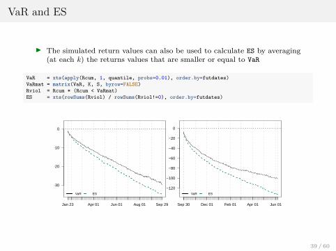
VaR and ES

I The simulated return values can also be used to calculate ES by averaging(at each k) the returns values that are smaller or equal to VaR

VaR = xts(apply(Rcum, 1, quantile, probs=0.01), order.by=futdates)VaRmat = matrix(VaR, K, S, byrow=FALSE)Rviol = Rcum * (Rcum < VaRmat)ES = xts(rowSums(Rviol) / rowSums(Rviol!=0), order.by=futdates)

Jan 23 Apr 01 Jun 01 Aug 01 Sep 29

−30

−20

−10

0

VaR ES

Sep 30 Dec 01 Feb 01 Apr 01 Jun 01

−120

−100

−80

−60

−40

−20

0

VaR ES

39 / 60

Filtered Historical Simulation (FHS)

I A drawback of HS is that it adapts very slowly to changes in asset volatility

I An alternative that has been proposed is Filtered Historical Simulation(FHS) which combines features of parametric modeling, MC, and HS

I FHS assumes:

1. A time-series volatility model for returns, e.g., Rt+1 = σt+1εt+1,where σt+1 is assumed to follow a GARCH model

2. No error distribution is assumed; instead, the simulated errors εs,t+kare random draws from the standardized returns Rt+1/σt+1

3. 1 and 2 are used in a MC simulation as shown above

40 / 60

I The only difference between MC and FHS consists of the distributionassumed to draw the simulated errors: a parametric distribution in the caseof MC (standard normal or td) or the empirical distribution of thestandardized returns (Rt+1/σt+1)

I This implies that the resampled εs,t+k maintain the features of the data,such as skewness and kurtosis

I In R this is implemented by drawing the εs,t+k by sample(std.resid, S,replace=TRUE) instead of rnorm(S) (or rt(S, df))

I In the next plots we compare the expected one-day volatility and the 99%VaR based on the k-period cumulative return conditional on January 22,2007 and September 29, 2008

41 / 60

# standardized residualsstd.resid = as.numeric(residuals(fitgarch, standardize=TRUE))std.resid1 = as.numeric(residuals(fitgarch1, standardize=TRUE))

for (i in 2:K){

Sigma.fhs[i,] = (gcoef[’omega’] + gcoef[’alpha1’] * R.fhs[i-1,]^2 +gcoef[’beta1’] * Sigma.fhs[i-1,]^2)^0.5

R.fhs[i,] = sample(std.resid, S, replace=TRUE) * Sigma.fhs[i,]Sigma.fhs1[i,] = (gcoef1[’omega’] + gcoef1[’alpha1’] * R.fhs1[i-1,]^2 +

gcoef1[’beta1’] * Sigma.fhs1[i-1,]^2)^0.5R.fhs1[i,] = sample(std.resid1, S, replace=TRUE) * Sigma.fhs1[i,]

}

Jan 232007

Mar 012007

May 012007

Jul 012007

Sep 012007

0.4

0.6

0.8

1.0

Expected Volatility

MC FHS

Sep 302008

Dec 012008

Feb 012009

Apr 012009

Jun 012009

1.0

1.5

2.0

2.5

3.0

Expected Volatility

MC FHS

Jan 23 Mar 01 May 01 Jul 01 Sep 01

−30

−20

−10

0

Cum. Returns − 99% VaR

MC FHS

Sep 30 Dec 01 Feb 01 Apr 01 Jun 01

−120

−100

−80

−60

−40

−20

0

Cum. Returns − 99% VaR

MC FHS

42 / 60

Portfolio VaR

I In practice, the portfolio of large financial institutions is composed of severalassets and its return can be express as

Rp,t =J∑

j=1

wj,tRj,t

where:I Rp,t represents the portfolio return in day tI wj,t is the weight of asset j in day t (and there is a total of J assets)I Rj,t is the return of asset j in day t

I Let’s assume that the bank holds only 2 assets (i.e., J = 2)

I The expected portfolio return is given by: E(Rp,t) = µp,t = w1,tµ1 + w2,tµ2

I The portfolio variance is given by:Var(Rp,t) = σ2

p,t = w21,tσ

21 + w2

2,tσ22 + 2w1,tw2,tρ12σ1σ2

which is a function of the individual variances and the correlation betweenthe two assets, ρ12

43 / 60

I The portfolio Value-at-Risk is then given by

VaR1−αp,t = µp,t + zασp,t

= w1,tµ1 + w2,tµ2 + zα√

w21,tσ

21 + w2

2,tσ22 + 2w1,tw2,tρ12σ1σ2

I If we assume that µ1 = µ2 = 0, the VaR1−αp,t formula can be expressed as

follows:

VaR1−αp,t = +zα

√w2

1,tσ21 + w2

2,tσ22 + 2w1,tw2,tρ12σ1σ2

= −√

z2αw2

1,tσ21 + z2

αw22,tσ

22 + 2 ∗ z2

αw1,tw2,tρ12σ1σ2

= −√

(VaR1−α1,t )2 + (VaR1−α

2,t )2 + 2 ∗ ρ12VaR1−α1,t VaR1−α

2,t

and:

1. if ρ12 = 1: VaR1−α1,t + VaR1−α

2,t2. if ρ12 = −1: −|VaR1−α

1,t −VaR1−α2,t |

3. if −1 < ρ12 < 1:VaR1−α

1,t + VaR1−α2,t < VaR1−α

p,t < −|VaR1−α1,t −VaR1−α

2,t |

44 / 60

I If we assume that the mean and the variance vary over time then VaR1−αp,t is:

VaR1−αp,t = w1,tµ1,t+w2,tµ2,t+zα

√w2

1,tσ21,t + w2

2,tσ22,t + 2w1,tw2,tρ12,tσ1,tσ2,t

where:I µ1,t = β0 + β1R1,t−1 and µ2,t = β0 + β1R2,t−1I σ2

1,t , σ22,t MA, EMA, and a GARCH

I ρ12,t ??

45 / 60

Modeling correlations

I A simple approach to modeling correlations consists of using MA and EMAsmoothing as in the case of modeling volatility

I Denote the returns of asset 1 by R1,t and of asset 2 by R2,t

I The MA(M) estimate of the covariance of the two assets is:

σ12,t+1 =1M

M∑m=1

R1,t−m+1R2,t−m+1

I The correlation is then given by: ρ12,t+1 = σ12,t+1/ (σ1,t+1 ∗ σ2,t+1)

I If the portfolio is composed of J assets there are J ∗ (J − 1)/2 correlations toestimate

I An alternative approach is to use EMA smoothing which can beimplemented using the recursive formula discussed earlier:

σ12,t+1 = (1− λ)σ12,t + λR1,tR2,t

and the correlation can be obtained as earlier by dividing with the standarddeviation forecasts.

46 / 60

Application in R

I We hold a portfolio that is invested for a fraction w1 in a gold ETF (ticker:GLD) and the remaining fraction 1− w1 in the S&P 500 ETF (ticker: SPY)

I The data are from January 02, 1970, January 02, 1970 until January 03,1970, January 02, 1970 at the daily frequency

I I will forecast volatility and correlation using the EMA approach withλ = 0.94

data <- getSymbols(c("GLD", "SPY"), from="2005-01-01")R <- 100 * merge(ClCl(GLD), ClCl(SPY))names(R) <- c("GLD","SPY")# EMA for the product of returnsprod <- R[,1] * R[,2]cov <- EMA(prod, ratio=0.06)# EMA for the squared returnssigma <- do.call(merge, lapply(R^2, FUN = function(x) EMA(x, ratio=0.06)))^0.5names(sigma) <- names(R)# correlation given by covariance divided by product of the st. dev.corr <- cov / (sigma[,1] * sigma[,2])

47 / 60

autoplot(corr) + geom_hline(yintercept=0, color="tomato3", linetype="dashed") +geom_hline(yintercept = as.numeric(cor(R[,1], R[,2], use="pairwise.complete"), color="seagreen4", linetype="dashed")) +theme_bw() + labs(x=NULL, y=NULL)

−0.5

0.0

0.5

2005 2010 2015

48 / 60

I VaR for a portfolio investing w1 in GLD and 1− w1 in SPY

w1 = 0.5 # weight of asset 1w2 = 1 - w1 # weight of asset 2VaR = -2.33 * ( (w1*sigma[,1])^2 + (w2*sigma[,2])^2 +

2*w1*w2*corr*sigma[,1]*sigma[,2] )^0.5autoplot(VaR) + geom_hline(yintercept=0, color="tomato3", linetype="dashed") +

theme_bw() + labs(x=NULL, y=NULL)

−8

−6

−4

−2

0

2005 2010 2015

49 / 60

I A comparison of portfolio VaR with VaR for a portfolio that is fully investedin GLD or SPY

VaRGLD = -2.33 * sigma[,1]VaRSPY = -2.33 * sigma[,2]mydata <- merge(VaR, VaRSPY, VaRGLD)autoplot(mydata, facets=FALSE) + theme_bw() +

geom_hline(yintercept=0, color="tomato2", linetype="dashed")

−10

−5

0

2005 2010 2015

plot_group

GLD

GLD.1

SPY

50 / 60

Backtesting VaR

I What makes a risk model a good model?

I We need to identify some characteristics which should hold if our model isthe true one and test them on the data

I Backtesting means testing the goodness of our risk model in terms of threeproperties of the violations process, Vt+1, defined as

V 1−αt+1 = I (Rt+1 ≤ VaR1−α

t+1 )

where I (A) takes value 1 if the statement A is true, and 0 otherwiseI These properties are:

I Unconditional Coverage: we expect that 100 ∗ (1− α)% VaR isviolated 100*α% of the days

I Independence: violations should be independent over timeI Conditional Coverage: independent of what happened the previous

day, we should always have a 1% chance of having a violation

51 / 60

I For the S&P 500 example above with volatility predicted using EMA andα = 0.01 we have:

T1 = sum(V)TT = length(V)alphahat = T1 / TTround(alphahat,3)

[1] 0.011

I The fraction of days with violations is 1.079% which is different from theexpected value of α = 1%

I Significantly different? We want to evaluate this hypothesis statistically bytesting the null that H0 : α̂ = α

52 / 60

Unconditional Coverage (UC) test

I The violation r.v. V 1−αt+1 (for t = 0, · · · ,T − 1) is a binomial random

variable with probability α, that is,

P(V 1−αt+1 = 1) = α

andP(V 1−α

t+1 = 0) = 1− α

I Example: let’s say that we have only three days and in the second day therewas a violation, but not in the other days

I V1 = 0,V2 = 1,V3 = 0 and the probability of this event is

P(V1 = 0,V2 = 1,V3 = 0) = (1− α)1 ∗ α0︸ ︷︷ ︸P(V1=0)

∗ (1− α)0 ∗ α1︸ ︷︷ ︸P(V2=1)

(1− α)1 ∗ α0︸ ︷︷ ︸P(V3=0)

so thatP(V1 = 0,V2 = 1,V3 = 0) = (1− α)2α1

I More generally, if we have a sample of T days with T1 days with a violation(V 1−α

t+1 = 1) and T0 without a violation (V 1−αt+1 = 0), the joint probability of

the sequence of violation is given by

L(α,T1,T) = αT1 (1− α)T0

53 / 60

I The UC test is performed by comparing the likelihood above calculated atthe theoretical probability 0.01 with the likelihood calculated at theestimate of α, α̂ = T1/T

I The statistic and distribution of the test for Unconditional Coverage(UC) are

UC = −2 ln(L(α,T1,T)L(α̂,T1,T)

)∼ χ2

1

where α is the level at which VaR was calculated, α̂ = T1/T and χ21 denotes

the chi-square distribution with 1 degree-of-freedom.

I The critical values at 1, 5, and 10% are 6.63, 3.84, and 2.71, respectively

I The null hypothesis H0 : α̂ = α is rejected if UC is larger than the criticalvalue

54 / 60

I In practice, the test statistic can be calculated as follows:

−2[T1 ln

(α

α̂

)+ T0 ln

(1− α1− α̂

)]In the example discussed above we have α̂ = 0.01, T1 = 74, and T is 6860.The test statistic is thus 0.42

I Since 0.42 is smaller than 3.84 we do not reject at 5% significance level thenull hypothesis H0 : α̂ = α and conclude that the risk model providesappropriate unconditional coverage

55 / 60

Independence

I Another property that we would like the risk model to satisfy is thatviolations happen at random times

I This property does not hold when violations happen in consecutive days

I To test this hypothesis we calculate two quantities:

1. α1,1: the probability of a violation in day t given that a violationoccurred in day t − 1 (and α1,0 = 1− α1,1 probability of no violationin t given the violation the previous day)

2. α0,1: the probability of having a violation in day t given that noviolation occurred the previous day (and α0,0 = 1− α0,1 )

I They can be estimated from the data by calculating T1,1 and T0,1 thatrepresent the number of days in which a violation was preceded by aviolation and a no violation, respectively.

56 / 60

I In R we can determine these quantities as follows:

T11 = sum((lag(V)==1) & (V==1))T01 = sum((lag(V)==0) & (V==1))

I The results are:I T0,1 = 74 and T0,0 = 6711I T1,1 = 0 and T1,0 = 74

I The conditional probabilities are then given by:I α̂0,1 = T0,1/(T0,1 + T0,0) = 0.011 and α0,0 = 1− α0,1I α̂1,1 = T1,1/(T1,0 + T1,1) = 0 and α1,0 = 1− α1,1

57 / 60

I The likelihood of observing T0,1 and T1,1 sequences out of T is given by

L(α̂0,1, α̂1,1,T0,1,T1,1,T) = α̂T1,01,0 (1− α̂1,0)T1,1 α̂

T0,10,1 (1− α̂0,1)T0,0

I The IND test statistic is calculated as

IND = −2 ln(

L(α̂,T0,T)L(α̂0,1, α̂1,1,T0,1,T1,1,T)

)∼ χ2

1

where:I the numerator is the same as the denominator in the UC test and

represents the likelihood under independenceI The logarithm of the denominator is calculated as:

T1,0lnα1,0 + T1,1ln(1− α1,0) + T0,1 lnα0,1 + T0,0 ln(1− α0,1)

I The test statistic and distribution for the hypothesis of Independence(IND) in this case is 1.61 which is smaller relative to the critical value at5% and we conclude that we do not reject the null hypothesisH0 : α0,1 = α1,1 = α̂. The violations are independent.

58 / 60

Conditional coverage

I In this case the hypothesis that we are interested in testing isH0 : α0,1 = α1,1 = α

I CC tests jointly independence of the violations and that coverage is alwaysequal to 1%

I The test statistic is calculated as CC = LRIND + LRUC ∼ χ22

I The critical value at 5% is 5.99 and the test statistic is 2.03 so that we donot reject the null hypothesis of correct conditional coverage.

59 / 60

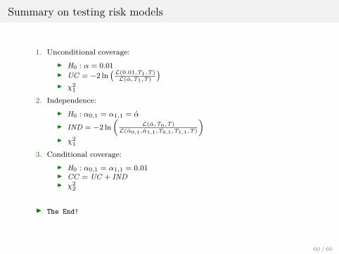
Summary on testing risk models

1. Unconditional coverage:I H0 : α = 0.01I UC = −2 ln

(L(0.01,T1,T)L(α̂,T1,T)

)I χ2

1

2. Independence:I H0 : α0,1 = α1,1 = α̂

I IND = −2 ln(

L(α̂,T0,T)L(α̂0,1,α̂1,1,T0,1,T1,1,T)

)I χ2

1

3. Conditional coverage:I H0 : α0,1 = α1,1 = 0.01I CC = UC + INDI χ2

2

I The End!

60 / 60