SERIEs (2015) 6:361–405DOI 10.1007/s13209-015-0136-z

ORIGINAL ARTICLE

Measuring expectations from household surveys: newresults on subjective probabilities of future house prices

Olympia Bover1

Received: 30 October 2015 / Accepted: 11 November 2015 / Published online: 26 November 2015© The Author(s) 2015. This article is published with open access at Springerlink.com

Abstract I analyze new data on subjective probabilistic expectations on house pricescollected in the Spanish Survey of Household Finances. Households are asked to dis-tribute ten points among five different scenarios for the change in the price of theirhomes over the next 12 months. This paper is the first empirical study to document thebeliefs of a representative sample of households about the future value of their homes. Italso reviews the methodology of expectation measurement and recent work on house-hold subjective probabilities. I model individual subjective probability densities usingsplines, construct quantiles from those densities, and analyze how the heterogeneityin the individual distributions relates to differences in housing and household char-acteristics. An important result of the paper is that women are more optimistic aboutthe evolution of house prices than men. Location at the postal code level accountsfor a large fraction of the variation in the subjective distributions across households.Finally, I provide some results on how subjective expectations matter for predictingspending behavior. Housing investment and car purchases are negatively associatedwith pessimistic expectations about future house price changes and with uncertaintyabout those expectations.

Keywords Household subjective probabilistic expectations · House priceexpectations · Gender bias · Consumption · Portfolio decisions

JEL Classification C81 · D84 · D12 · D14 · R21

This paper was written as a lecture for presentation as the Presidential Address to the Congress of theSpanish Economic Association in Vigo, December 2012. I am grateful to an anonymous referee and theEditor for their helpful comments.

B Olympia Boverbover@bde.es

1 Banco de España, Madrid, Spain

123

362 SERIEs (2015) 6:361–405

1 Introduction

This lecture is concerned with household subjective expectations. Its central themeis the analysis of new data on subjective probabilistic expectations on house pricescollected in the Spanish Survey of Household Finances (EFF). As a front-end, I firstprovide a review of the methodology of expectation measurement and of some recentwork that use household subjective probabilities. Finally, as a back-end I provide someresults on how subjective expectations matter for predicting consumption behavior.

Despite widespread agreement on the fundamental role of expectations in explain-ing behavior, direct measurement of individual expectations is a relatively recentactivity. The standard practice in the economics of the last century was to infer theindividuals’ decision process from their observed choices. Following this revealedpreference analysis, both preferences and the uncertainty about the future are identi-fied from data on choices and market outcomes alone. Such strategy requires strongassumptions. For example, assuming individuals have rational expectations as well asknowledge of the model may be needed despite that this has often not been credible. Inhis seminal paperManski (2004) strongly advocated for collecting self reported expec-tation data and using those jointly with observed choice data. The hope is this wouldimprove economists’ credibility and ability to predict behavior. But are householdexpectations collected through surveys trustworthy? Do subjective household surveyexpectations really improve the ability to predict behavior? To help put these ques-tions in context, I begin by reviewing basic concepts of themethodology of expectationmeasurement as well as recent work on the elicitation and use of household subjectiveexpectations.

The EFF is a representative survey of the Spanish population that contains detailedinformation on household assets, debts, income and consumption. Data have beencollected every three years since 2002. Starting in 2011, the EFF introduced a newquestion to elicit household house price probabilistic expectations. Households wereasked to distribute ten points among five different scenarios concerning the pricechange of their homes over the next 12 months. In this way respondents provideinformation not only about point expectations but also about the probabilities theyassign to different future outcomes.

One motivation for introducing this question in the EFF is the importance of realestate assets in the wealth of Spanish households (80 % of the value of householdassets) all along the wealth distribution (88 % for the bottom quartile and 67.5 % forthe top decile). Aside from a high proportion of owner occupier households (83 %),36 % of Spanish households hold some other real estate property.

It is also a timely question due to the housing market collapse that shattered houseprice expectations after 2007 in Spain. The number of households buying housingdropped dramatically from an overall annual average rate of 2.3 % between 2002 and2005 to 1.1 % in 2011. According to the data I analyze in this paper, in 2011 over 23%of households expected a large drop (of over 6 %) in the future price of their homes.Moreover, among households expecting such large drops, the fraction who bought acar was half the fraction in the total population (4.5 instead of 9.4 %).

This paper is one of the first empirical studies to document the beliefs of householdsabout the future value of their homes, and the first one that uses a representative

123

SERIEs (2015) 6:361–405 363

sample of households. Questions on probabilistic house price expectations have onlyrecently been introduced in household surveys, as detailed in Sect. 3. Niu and vanSoest (2014) have independently obtained results that are complementary to oursusing newly collected house price expectations data from the Rand American LifePanel.

I start by analyzing patterns of the answers provided by the EFF2011 respondents tothe house price probabilistic expectation question to assess the coherency of responses.These include bunching, number of intervals used, and their associationwith the extentof non-response. Next I model individual probability densities and analyze how theheterogeneity in the individual distributions relates to differences in housing propertiesand in the characteristics of households.

An important result of the paper is that women are more optimistic about theevolution of house prices than men. Being a woman is associated with a positive shiftin the median and the quartiles of the subjective distributions. I further examinedpotential differences in asset valuations by gender by considering self-assessed valuesof other assets reported in the EFF. I find that women tend to provide higher estimatesfor the value of their home compared to men but lower ones when it comes to valuetheir financial assets.

Location at the postal code level accounts for a large fraction of the variation inthe subjective distributions across households. Importantly, in the absence of postalcode fixed effects the estimated effects of demographics on house price expectationswould be biased. For example, the result on gender would not be found. Moreover,the location effects that emerge from the subjective probability data are meaningfuland respond to economic fundamentals. In particular, estimated location fixed effectsrespond to past local house prices and unemployment rates.

Finally, I study whether reported household expectations predict household expen-diture decisions. This is of substantive interest to understand household behavior andalso a further step in the validation of the house price expectation responses. I exploitthe availability in the EFF of information about purchases of secondary housing, cars,other big ticket items, and food. These data allow me to uncover some novel find-ings about correlations of house price expectations and their uncertainty with thosepurchases and expenditures. I find that housing investment and car purchases are neg-atively associated with pessimistic expectations about future house price changes andwith uncertainty about those expectations. Moreover, these effects depend on house-hold wealth. Specifically, the negative effects of holding very pessimistic house priceexpectations on secondary housing purchases are more pronounced at the top of thewealth distribution than at the median, while the opposite is true for car purchases.

The paper is structured as follows. In Sect. 2 the work on elicitation and use ofhousehold expectations is reviewed. I discuss the specificities in implementing expec-tation questions in household surveys and the validation of such questions. I alsodiscuss some specific uses of subjective expectations, work on expectation formation,and some enlightening experiments conducted within expectation surveys. Section 3contains the analysis of the house price expectations data in the EFF. First I describethe formulation of the question and I examine the quality of the responses. Next Iestimate a probability density for each respondent, which I use to document the extentof heterogeneity in beliefs. Based on these individual densities I compute various

123

364 SERIEs (2015) 6:361–405

quantiles and measures of dispersion, and study their association with respondentand house characteristics. Finally, Sect. 4 reports the results on the relation betweenhouse price expectations and expenditure decisions. I present predictive results forthe probabilities of purchasing secondary housing, an automobile, and other big ticketitems.

2 The quantification of human uncertainty from social surveys

2.1 Preliminaries

After years of distrust, the measurement of individual expectations is becoming a veryactive topic in economics, both for research and for immediate policy use. Since the1990s an increasing number of household surveys have been collecting data on subjec-tive probabilistic expectations.1 Expectation questions may be about future outcomesconcerning the individual (e.g. own income, health, death, job security, home value,pension benefits, bequests) or about future aggregate conditions (e.g. inflation, houseprices, stock market).

There are two important distinctions when considering asking expectations ques-tions. First, whether the question is about eliciting point expectations as, for example,asking for the expected number of children, or about eliciting probabilistic expecta-tions. A probabilistic counterpart to the previous example would be to ask about theprobability of having no children, of having one child, of having two children, etc.

The second important distinctionwhen considering eliciting expectations iswhetherthe answer we seek is qualitative or quantitative. Qualitative questions to measureexpectations have been used for some time. An example of qualitative question is asfollows:

“Thinking about the next 12 months how likely do you think it is that you will loseyour job? Possible answers: very likely, fairly likely, not too likely, not at all likely”.

An alternative probabilistic question on the same subject is:“Using a scale from 0 to 100 what is the percent chance that you lose your job in

the next 12 months?”.This type of probabilistic questions are usually preceded by some explanations and

examples about themeaning of probabilities (e.g. using examples about the probabilityof rain) and/or accompanied by some visual aid (e.g. a ruler).

Two limitations of verbal expressions of expectations (of the type “very likely”,“fairly likely”, “not too likely”) are that different respondents may interpret them dif-ferently and that they convey limited information about respondents’ expectations. Infact, Dominitz and Manski (1997, 2004) blame the early use of verbal expectationsfor the economists’ distrust of expectations data. In particular, they cite a controversyin the 1950s and 1960s about the usefulness of elicited verbal assessments of expectedconsumer finances in the Federal Reserve Board Survey of Consumer Finances con-

1 Some of the most prominent are the US Health and Retirement Survey (HRS) and its UK counterpart theEnglish Longitudinal Study of Ageing (ELSA), the US Survey of Economic Expectations, the AmericanLife Panel (ALP), some Household Wealth Surveys (in particular the Italian SHIW, the Dutch VSB Panel,and the Spanish EFF).

123

SERIEs (2015) 6:361–405 365

ducted by the University ofMichigan Survey Research Center. The debate had GeorgeKatona2 as the leading proponent of qualitative attitudinal questions vs. Thomas Justerwho did not find them useful in predicting behavior.3 This debate would have lefteconomists suspicious of any expectation data for a while.

The advantages of asking probabilistic expectations are that numeric answers arecomparable across persons and over time, algebramay be used to examine consistency,and they allow respondents to express uncertainty or risk.

Measuring probabilistic expectations about future continuous outcomes entailsobtaining each respondent’s subjective probability distribution. An early example isthe following question about earnings uncertainty included in the 1989 Survey ofHousehold Income and Wealth (Banca d’Italia):

“We are interested in knowing your opinion about labor earnings or pensions12 months from now. Suppose now that you have 100 points to be distributed betweenthese intervals (a table is shown to the person interviewed). Are there intervals whichyou definitely exclude? Assign zero points to these intervals. Howmany points do youassign to each of the remaining intervals?”.

A different formulation with the same objective could be“How likely do you think it is that your income in the coming year will be higher

than ___ (A/B/C) Rupees?”as adopted in Attanasio and Augsburg (2012), where A, B, and C are different

income thresholds. The information is elicited in the form of a probability density inthe first case and of a cumulative distribution in the second.

Despite some potential added difficulty for the respondent in answering questions ina probabilistic form,most of the evidence shows that respondents are willing to answerprobabilistic questions and that their responses are generally sensible and internallyconsistent. This is so when the questions concern well defined events that relate torespondents’ lives (see for example evidence cited in Manski 2004; van der Klaauwet al. 2008).

Recently probabilistic expectations data have also been collected in developingcountries (see Attanasio 2009; Attanasio and Augsburg 2012) where getting sensibleanswers to such questions has also proved feasible. Some controversy however remainsrelated to Tversky and Kahneman (1974) randomized experiments, which reveal thatindividuals often use heuristic methods rather than Bayes theorem.

Studies on decision making under ambiguity take probability expectations one stepfurther. Ambiguity arises when individuals do not hold a single subjective distributionbut may hold a set of them. In the case of binary events this would translate into

2 See Katona (1957).3 See Juster (1964, 1966) proposed eliciting probabilistic expectations by linking verbal expressions withnumerical probabilities. His formulation of a purchase probability question regarding automobiles and otherhousehold appliances reads as follows (as reported in Manski 2004):Taking everything into account, what are the prospects that some member of your family will buy a ___sometime during the next ___ months, between now and ___?Certainly, Practically Certain (99 in 100); Almost Sure (9 in 10); Very Probably (8 in 10); Probably (7 in10); Good Possibility (6 in 10); Fairly Good Possibility (5 in 10); Fair Possibility (4 in 10); Some Possibility(3 in 10); Slight Possibility (2 in 10); Very Slight Possibility (1 in 10); No Chance, Almost No Chance (1 in100).

123

366 SERIEs (2015) 6:361–405

allowing answers in intervals of probabilities instead of only point probabilities (foran extended explanation see Manski 2004). Manski (2004) provides the followingexample in the case of binary events: “What do you think is the percent chance thatevent A will occur? Please respond with a particular value or a range of values, as yousee fit”. He comments that this formulation enables respondents to express uncertaintyor ambiguity. For example, complete ignorance may be expressed by reporting “0–100%”, bounded ambiguity by reporting “30–70%”, uncertainty by reporting “60%,”or certainty by reporting “100 %”.

2.2 Elicitation methodology

Asking for uncertainty requires a process of elicitation. It is not like asking for age.Hence elicitationmethodsmatter to what gets elicited. Understanding this is importantbut does not necessarily render the request for elicitation meaningless.

Wording A substantial amount of work has been produced to try to minimize biasand systematic error by refining the way information is elicited. This is relevant sinceeven apparently minimal differences in wording may produce different interpretationsof the question.

A salient example is the experiment conducted by the Federal Reserve Bank ofNew York, as part of their Household Inflation Expectations Project, on the effectsof alternative wordings for eliciting inflation expectations. One conclusion is thatreported expectations were higher when the question asked was about expectationsof “prices in general” (as in the long standing Michigan Survey question) than whenthe formulation was in terms of “inflation” expectations (see for example Bruine deBruin et al. 2011b, 2012). These authors report that question about “prices in general”and “prices you pay” focus respondents more on personal price experience and sincethese may be driven by prices of different goods over time the answers may be lesscomparable than the ones prompted by an “inflation” formulation.

More generally, the wording used in eliciting subjective probabilities has to con-vey the concept of probability in a manner the respondent understands, so that heis able to express his probabilistic beliefs. In developed countries the usual wordingis “percent chance” or “how likely”, while in developing countries respondents areoften given a number of beans or balls they are asked to distribute.4 Delavande et al.(2011) compare distributing balls across bins to the percent chance approach. In theirIndian setting beans generate usable answers for almost all respondents while a per-cent chance formulation produced a significant fraction of inconsistent answers.5 Apractical consideration is the number of beans respondents are given to distribute.Greater accuracy may be expected the larger this number is but with too many beanseventually proving difficult to handle by the respondent.

4 But see Delavande and Rohwedder (2011) who ask Internet respondents in the US to allocate 20 ballsacross seven bins to express their beliefs about their future Social Security benefits.5 Along the same lines, Manski (2004) reports evidence that respondents perform much better when sta-tistics are presented in the form of natural frequencies (e.g. 30 out of 10,000 cases) rather than in the formof objective probabilities (0.3 % of cases).

123

SERIEs (2015) 6:361–405 367

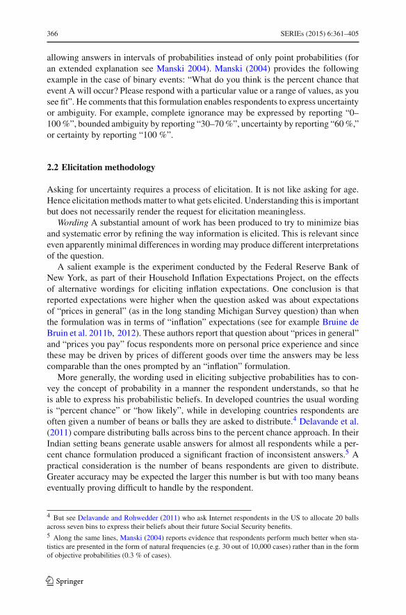
Visual aids are often employed to help respondents. In particular, a ruler may beused to explain the percent chance scale from 0 to 100 %. Visual aids have also provenuseful in internet administered surveys in the US (see Delavande and Rohwedder2011).6 Often, time is also spent in providing examples about probability statements(for example, the probability of rain tomorrow) to try and make sure respondentsunderstand probabilistic statements.7

Eliciting subjective distributions: range of variation Various elements need to bespecified when formulating questions to obtain subjective distributions. The first con-sideration is to establish the range of variation of the outcome of interest. This maybe obtained by asking the respondent to report the maximum and minimum possibleoutcome in a couple of preliminary questions. Alternatively the support may be chosenby the developer of the questionnaire and to be the same for all respondents.8 The firstoption is now routinely used when the outcome is household or individual specific(e.g. own income) because it decreases the natural focus of the respondent on centraltendencies and avoids that pre-established reference values influence his answers (alsoknown as anchoring problem).9 Predetermined ranges are predominant when elicitingexpectations about aggregate outcomes (e.g. inflation). Once the range of variation isestablished it is divided in intervals (not necessarily equally wide) and correspondingcut-off points are determined. Presenting a large number of intervalsmay subsequently

6

7 In the Health and Retirement Survey for example the explanations given are as follows:“Next we wouldlike to ask your opinion about how likely you think various events might be. When I ask a question I’d likefor you to give me a number from 0 to 100, where “0” means that you think there is absolutely no chance,and “100” means that you think the event is absolutely sure to happen. For example, no one can ever besure about tomorrow’s weather, but if you think that rain is very unlikely tomorrow, you might say that thereis a 10 % chance of rain. If you think there is a very good chance that it will rain tomorrow, you might saythat there is an 80 % chance of rain”.8 Dominitz andManski (1997) warn against interpreting the answers onminimum andmaximum outcomesas absolute minimum and maximum possible outcomes and recommend using these only to help determinethe range as opposed to fully determine it. Their suggestion would help overcome the problem discussed inDelavande et al. (2011) that self-reported ranges often produce less rounded interval bounds than would bethe case with predetermined support. Non-rounded intervals are likely to be harder to think about for therespondent.9 See Delavande et al. (2011) for an attempt to compare the sensitivity of the results to differences in thespecification of support.

123

368 SERIEs (2015) 6:361–405

allow for more precise statistics but bemore cognitively demanding on the respondent.More intervals may be needed for individual outcomes with predetermined supportsthan with self-anchored ones to allow for individual heterogeneity in outcomes.10

Eliciting subjective distributions: cdf vs. pdf A third consideration when devisingsubjective distribution questions is whether to elicit the information in the form ofa probability density (pdf) or a cumulative distribution (cdf). With a pdf format therespondent is faced with assessing the probabilities that the outcome lies in each inter-val (e.g. the 1989 SHIW question cited earlier) while with a cdf format he has toassess the probabilities that the outcome does not exceed the sequence of thresholds(e.g. as in Attanasio and Augsburg 2012; also the question cited in the introduc-tion).

Most studies have been eliciting cdfs although lately an increasing number of ques-tions are being framed as pdfs (for examples of pdf questioning see Arrondel et al.2011, the NewYork Federal Reserve inflation question in Bruine de Bruin et al. 2011b;Delavande et al. 2011).Morgan andHenrion (1990) cite experimental evidence report-ing that individuals find it easier to deal with pdfs that allow an easier visualizationof certain properties of the distribution like location and symmetry. Traditionally, thelarger probabilities involved in cdfs was thought to help respondents.

An alternative to eliciting probabilities in the form of cdfs or pdfs is to ask forquantiles of the distribution, for example, the respondent is prompted to provide avalue X such that there is a 25 % chance of her income being less than X. Early onboth Morgan and Henrion (1990) and Dominitz and Manski (1997) rejected elicit-ing quantiles citing evidence that probabilities assessed in this way match less wellempirical frequencies.

Last but not least, knowledge about the subject matter There are two basic consid-erations for successfully eliciting probabilistic expectations. The respondent shouldhave knowledge about the event or outcome to be assessed as well as some skillsin expressing beliefs in probabilistic form.11 Although the later condition may oftenseem difficult to satisfy, there have been advances in learning forms of elicitationthat may be easier for the respondent as we have discussed above. However, lack ofknowledge about the subject matter may prove more difficult to overcome. This maybe the case, for example, when trying to elicit stock market return expectations fromlow income and low education households. For many people mutual fund returns arenot part of their lives and hence they lack knowledge of the subject matter which isa necessary condition for individuals to be able to express meaningful beliefs aboutit. Subjects in general know a lot about themselves but much less about aggregatecircumstances.

10 Delavande et al. (2011) use 20 intervals with predetermined support and four with a self-anchored onewhen eliciting expectations about the respondent’s expected fish catch. Attanasio and Augsburg (2012)work with four intervals and self-anchored support when eliciting the cdf of expected individual income.Both studies were done in India. Hurd et al. (2011) and van der Klaauw et al. (2008) elicit expectationsabout aggregate variables (Dutch stock returns and US inflation, respectively) and define eight intervalswith predetermined support.11 See Delavande et al. (2011) for examples of supporting evidence.

123

SERIEs (2015) 6:361–405 369

2.3 Validation diagnostics

Response rates Individuals are willing to answer probabilistic expectation questions.Response rates inmany cases are high (e.g. 97% inAttanasio andAugsburg 2012, 99%in Bruine de Bruin et al. 2011a, 79–87% in Hurd et al. 2011) and higher than for actualor historical outcomes in the same surveys. But non-response varies substantially withthe matter being elicited. For example, in the 2006 HRS non-response was 4 % forthe expected survival probability question but 24 % for the expected gain in the stockmarket.12

Coherence However, a major concern has been whether the answers obtained couldreally be interpreted as the respondent’s subjective beliefs about uncertain outcomes.Therefore, in all studies some time is spent analyzing coherence of the responses invariousways. In the first place, checks to verify compliancewith basic probability lawsare usually reported. Authors working with cdf formulation type questions report avarying degree of monotonicity violations. In some cases high compliance is achievedwith the help of a programmed automatic prompting in case of violation. Dominitzand Manski (1997) report around 10 % of monotonicity violations before the promptand 5 % afterwards while Attanasio and Augsburg (2012) report 1 % without the helpof such prompting. Automatic warnings for additivity violation (i.e. if probabilitiesor beans do not sum up to the required amount) in pdf questions are also useful.13

Bruine de Bruin et al. (2011a) report other checks to support the validity of responseslike the fraction of respondents who put positive probability mass in more than onebin (96.4 %) or the low fraction who put positive probability mass in non-contiguousbins (1.3 %) although some people may have bimodal beliefs.

Correlations and predictive power Correlations with other survey variables maysometimes provide information about the soundness of expectation answers. Attana-sio and Augsburg (2012) make use of the standard preliminary question about thelikelihood of rain. This question is often carried out to convey the idea of probabilityto respondents to further check the expected income distribution data they obtain fromhouseholds in rural India. They find a significant correlation between the answers tothe likelihood of rain and expected income for households whose main income isderived from agriculture and no significant correlation for those that do not. More rou-tinely, assessing how answers to subjective probabilities vary with socio-demographiccharacteristics of the respondent (i.e. compliance with prior beliefs about correlatesof expectations), is often seen as part of the validation of the data.

Predictive power is a desirable feature for the credibility of elicited expectations.However, beliefs may be inaccurate but nevertheless be the relevant measure behindobserved behaviour. In many different surveys individual expectations about stockmarket gains have been found to be substantially lower than what observed past (andfuture) averages would justify. Additionally, young educated males are found to sys-tematically holdmore optimistic expectations about the stockmarket than other groups

12 As expected, non-response is lower for stockholders (11 %) than for those not owning stocks (29 %).13 To some extent the need for prompts is a reflection of the limitations of the device used in implementingthe question. For example, a prompt would not be necessary if the respondents were actually given ten ballsto distribute using a mechanical or an electronic device.

123

370 SERIEs (2015) 6:361–405

(see Hurd 2009, for this and other examples). Moreover, beliefs about stock marketgains correlate with ownership of stocks.

Rounding Rounding of responses to the nearest 5 % is often reported although atthe tails respondents may round to the nearest 1 % (see for example Dominitz andManski 1997; Hudomiet et al. 2011; Attanasio and Augsburg 2012). Rounding maybe influenced to some extent by the design of the visual aid attached to the question,for example, marks on a ruler.

Epistemic uncertainty (ignorance about probabilities) More importance has beengiven to the bunching of responses at 50 % for the expected probability of a binaryevent (e.g. the percent chance of a positive stock market return or the probability for a70 years old person to live to at least the age of 80). Psychologists have reported thata 50 % reply may disguise a “don’t know” answer and reflect epistemic uncertainty,that is, the tendency to choose towards the middle of a scale when the respondent isnot able to provide an answer or does not understand the question. Alternatively, suchanswers could reflect a genuine belief that the event is equally likely to occur or notto occur (see Fischhoff and Bruine de Bruin 1999, for an early paper on the subject).

In order to disentangle responses that reflect a genuine probability belief from thosereflecting epistemic uncertainty some studies have included a follow up question in thecase of a 50 % answer. In 2006 the HRS added such an epistemic follow up questionto some of the probability questions, which revealed that, for example, the fraction of50 % answers to the survival probability question being simply ignorance (i.e. beingunsure about the chances) was as high as 60 %. The HRS formulation of the followup question for the percent chance of an increase in the value of mutual fund shareswas: “Do you think that it is about equally likely that these mutual fund shares willincrease in worth as it is that they will decrease in worth by this time next year or areyou just unsure about the chance?”.

In contrast, Dominitz and Manski (2007) provide some evidence that such answerscould reflect a genuine belief that the event is equally likely to occur or not to occur. Inparticular, they show that persons answering 50% to the 2004HRSquestion about theirperceived percent chance of a positive stock return hold more stocks than persons withlower expected probabilities but less than persons with higher expected probabilities.They infer therefore that such answers reflect a higher perceived chance of a positivestock return than less than 50 % answers but lower perceived chance of a positivestock return than more than 50 % answers.

Heaping Heaping at 0 and 100 reported but this is usually less problematic thanat 50 %. A high number of 0 and 100 responses probably reflects absence of precisebeliefs and therefore some uncertainty. However, they convey the information that thechances of the event occurring are thought to be extremely low or extremely high. Inany case focal answers at 0, 50, 100 reflect less precisely known probabilities thannon-focal ones. Lillard and Willis (2001) find that the tendency to give focal answersis associated with lower cognitive ability. Hurd et al. (2011) find in their data a fractionof “50 %-respondents” lower than in many other surveys and attribute this to the factthat Dutch CentER Panel members are experienced survey respondents.

In the context of eliciting expected distributions of continuous variables (either cdfor pdf formulation) too many answers of 0 % (100 %) chance of the outcome to be

123

SERIEs (2015) 6:361–405 371

higher than the lowest (highest) threshold may sometimes indicate that the chosenrange is not adequate.

Addressing Kahneman’s critique One critique to collecting subjective probabilisticexpectations is that respondents would not apply much effort and hence would notprovide thoughtful answers. In Kahneman’s dual system terminology, respondentswill tend to use intuition (system 1) and not reasoning (system 2). Gouret and Hollard(2011) take this criticism seriously and try to separate the fraction of respondentsthat do provide valuable information about expected mutual fund return distribution.To achieve this they construct a coherency measure and show that only for the mostcoherent individuals there is a significant monotonic relationship between expectedreturns and perceived risk. They find that their measure of coherency correlates witheducation and income.

In contrast, the results in Zafar (2011), analyzing a panel dataset of NorthwesternUniversity undergraduates that contains subjective expectations about major specificoutcomes, support the hypothesis that students exert sufficient mental effort whenreporting their beliefs.

However, in some cases, the problem may not lay in not exerting enough mentaleffort but in the wording of survey questions making it easy for some respondents toexpress their probability beliefs.

2.4 Some uses of subjective probability questions

An important motivation for introducing expectation questions in household surveysis to help explain household choices. Another still undeveloped use of individualresponses is the construction of statistics like, for example, statistics about inequalityin expected survival probabilities.14

Although there are already important studies that make use of subjective proba-bilities to explain economic behavior, a large proportion of the literature to date hasfocused on assessing the properties of the elicited information and establishing itsvalidity. Further to the basic validation checks described previously, this literature hasanalyzed variation in subjective probabilities across individuals and their predictivepower on outcomes.

To illustrate research work that uses subjective expectations survey data, I willbriefly review findings regarding three questions: survival probability, probability ofpositive stock return, and expected inflation distribution.15

Survival probability The expected probability of survival to age 75 was introducedearly on in the 1992HRS.16 Data from the first wave did show that the average survivalprobability was very similar to the 1990 survival rate from life tables. Once a second

14 It would be interesting for example to see if heterogeneity in household expected survival probabilitiesis very different to heterogeneity in realized mortality.15 See Manski (2004) and Hurd (2009) for more detailed reviews on uses of expectation questions.16 Other subjective probability questions introduced in the 1992 HRS wave dealt with expectations aboutretirement age, health limitations, inflation, health care expenditures, unemployment, housing prices, SocialSecurity benefits, giving financial help, and economic depression. A question about the expected probabilityof a positive stock return was added in 2002.

123

372 SERIEs (2015) 6:361–405

wave was available in 1994 subjective survival probabilities elicited in 1992 wereproved to be a good predictor of mortality for the period between the two waves. Thishas been also true in the European SHARE (see Winter 2008). Moreover, after fewyears, it was established that elicited survival probabilities and actual mortality datacorrelate with variables like education, wealth, income etc. in a similar way. In general,as Hurd (2009) points out, subjective probabilities have “predictive power” whenindividuals have considerable private information about the subject matter. Indeed,predictive power in itself may not be as interesting as indirectly getting insight aboutprivate information.

Some work has also been done on using expected survival probability to explaineconomic behaviour. For example, Hurd et al. (1998), using the survey of theAsset andHealth Dynamics among the Oldest Old (AHEAD), find that the probability of savingcorrelates in a significant and substantial way with individual subjective beliefs abouttheir own mortality risk but not, when jointly included, with life-table probabilities.Using the HRS, Hurd et al. (2004) study whether individuals who expect to be long-lived claim Social Security benefits later than those expecting to be more short-lived.Although they find effects in the expected direction, their size is modest in general butincreases with education. Finally, Gan et al. (2004) compare the ability of expectedsurvival probability in predicting out of sample wealth with life-tables using a life-cycle model of consumption.

Expectations about stock market return Subjective expectations about stock marketreturns have proven to be useful in helping resolve the stock holding puzzle. Under thetraditional assumption of rational and homogeneous expectations, observed low ratesof stockholding would be attributed to high risk aversion. However, elicited data showthat subjective stock return expectations are very heterogeneous and that this hetero-geneity helps explain participation in the stock market (while there is no evidenceof a risk aversion effect).17 Individuals having more optimistic beliefs about returnsare more likely to hold stocks. This effect was first found in Dominitz and Manski(2007) and has been confirmed by other authors in various contexts (Hurd et al. 2011;Hudomiet et al. 2011; Arrondel et al. 2011). Importantly, those heterogeneous beliefsseem to present systematic biases. Individuals are found to be more pessimistic aboutrates of return than the historical performance of the stock market (see evidence inHurd et al. 2011 for the Netherlands and Kézdi and Willis 2008, for the US) and menare consistently found to be more optimistic than women. Observed heterogeneity instock market expectations raises an important question about how beliefs are formedand what are the reasons behind such systematic differences given that informationabout stock prices is public and there is no private information.

Inflation expectationsHousehold expected inflation is assumed to feed into realizedprices if households take inflation into account when deciding about their purchase oflarge durables, saving instruments, wage negotiations, etc. Given this role of inflationexpectations in the monetary transmission mechanism it is widely agreed that in orderto control inflation it is important to learn about people’s beliefs concerning futureinflation.

17 Uncertainty about those expectations is also found to be heterogeneous when data about expecteddistributions are available.

123

SERIEs (2015) 6:361–405 373

For a long time many household surveys have asked point forecasts of expectedinflation (e.g. the Michigan Panel, the Bank of England/NOP Inflation AttitudesSurvey) but without eliciting related uncertainty.18,19 For example, the Bank of Eng-land/NOP survey question is the following:

“Howmuch would you expect prices in the shops generally to change over the next12 months?”.

In 2007 the Federal Reserve Bank of New York (FRBNY) began to develop asurvey to measure and analyse consumers’ inflation expectations.20 In this survey,carried out every six weeks approximately, the full expected distribution is elicitedasking respondents about the percent chance of inflation in the next 12 months beingin eight separate intervals. After instructions, the wording of the question is as follows:

“What do you think is the percent chance that, during the next 12 months, thefollowing things will happen? Prices in general will:

go up by 12% or more _____ percent chance

go up by 8 to 12%_____ percent chance

go up by 4 to 8%_____ percent chance

go up by 2 to 4%_____ percent chance

go up by 0 to 2%_____ percent chance

go down by 0 to 2%_____ percent chance

go down by 2 to 4%_____ percent chance

go down by 4% or more _____ percent chance

(100%Total)”

Armentier et al. (2013) present various validation diagnostics for this question. Fortheir experimental panel survey, non-response rate is less than half a percentage point,the proportion with positive probability in more than one bin is 89.4 % and the pro-portion with positive probability in non-contiguous bins is 1.6 %.

There is considerable heterogeneity across respondents in median forecasts whichare higher for respondents who are women, less educated, poorer, single, or older.When conditioning for all demographics only education remains significant but whenfurther controlling for financial literacy the effect of education is reduced.

Moreover, as we will see in detail below in Sect. 2.6, the authors find coherencybetween individual inflation expectations and financial choices. Related with the find-ings on the effect of education and literacy, these data reveal the inability of somegroups of the population to form sensible expectations. The results are also indicativeof the economic effects expectations of poor quality may have.

18 An exception is the Bank of Italy Survey of Household Income and Wealth who elicited the expectedinflation distribution in their 1989 and 1991 waves.19 There are also indirect ways to infer inflation expectations from the term structure of interest rates orfrom financial instruments but with some strong modelling assumptions.20 Until 2012 the survey was conducted over the internet with RAND’s American Life Panel.

123

374 SERIEs (2015) 6:361–405

Uncertainty about future inflation is positively related tomean andmedian expectedinflation.Moreover, using the panel dimension of the survey, respondentswho aremoreuncertain are found to make larger revisions to their expectations in the next survey(see Bruine de Bruin et al. 2011a; van der Klaauw et al. 2008).

2.5 Expectation formation

The availability of data on individual subjective expectations has prompted renewedinterest in analyzing their determinants and the amount of information households usewhen forming those expectations.

Testing for rational expectations There has been work with individual expectationsdata testing models of the way expectations are formed and in particular testing forrational expectations. When considering expectations over variables for which theindividual has substantial private information (e.g. educational attainment, mortalityrisk) and in some cases are under his control up to some extent (e.g. retirement age)the rational expectations hypothesis cannot be rejected.21 Benítez-Silva et al. (2008)test for rational expectations in the formation of retirement and longevity expectationsusing the Health and Retirement Study (1992–2002) and of educational attainmentexpectations using the National Longitudinal Survey of Youth (1979–2000). In theirframework this amounts to testing that differences in expectations in successive peri-ods cannot be forecast.22 Using instrumental variables for measurement error andaccounting for sample selection the authors cannot reject the rational expectationshypothesis.

Following a similar methodology Das and Donkers (1999) analyze the answersabout expected income growth in the Netherland’s Socio-Economic Panel but theyreject the hypothesis that these expectations are rational and find instead that house-holds are excessively pessimistic about their future income growth. However, the forceof the evidence is limited by the fact that expectations in that survey are elicited ina more qualitative way than in the HRS or the NLSY. In particular the set of pos-sible answers are: “strong decrease”, “decrease”, “no change”, “increase”, “strongdecrease”.

House price change is a relevant variable for the macroeconomy that has beenelicited in a few household surveys. The question may refer to house prices at thenational level or at a more disaggregate level (area, own house) for which householdsmay have more information. Case et al. (2012) test rationality of area house priceexpectations by regressing future house price change on the expected change.One-yearprice expectations are found to under-react to information while 10-year expectationsseem likely to have been over-reacting although this longer term rationality is stilldifficult to assess with the authors survey data for the 2003–2012 period.

Expectations about macro variables A recent literature on this topic has beenfocusing on the study of individual expectations (or “sentiment”) about macroeco-

21 For a detailed exposition of using survey expectation data for testing models of expectation formationsee Pesaran and Weale (2006).22 However, a model free test may not be easy to perform.

123

SERIEs (2015) 6:361–405 375

nomic variables where there is public information but no individual information (e.g.inflation, house prices, stock returns). In those cases expectations are found to besystematically biased and the literature has unveiled heterogeneity in various dimen-sions.23 Men, individuals who are young, highly educated, with high income are moreoptimistic and believe inflation will rise at a slower pace (Bruine de Bruin et al. 2010).However, these systematic biases in people’s expectations are not constant over time(Souleles 2004). Similar findings are obtained by looking at expected stock returns(Dominitz andManski 2007): there is variation in the empirical distributions over timeand men report higher expected returns than women (and the young higher than theold).

A relevant question is therefore what could explain these demographic differencesin expectations. Regarding inflation we have learned (see for example Bruine de Bruinet al. 2010) that inflation expectations are higher among respondents who thought rel-atively more about how to cover expenses and about specific prices, and among thosewith low financial literacy. Perceptions of past inflation are a major determinant ofinflation expectations (see Blanchflower and MacCoille 2009, using UK data) but thisis less so for individuals with high education. Cavallo et al. (2014) find that an indi-vidual’s expectations are influenced both by inflation statistics and supermarket pricesalbeit more by the latter that are less costly to understand. Another finding regardingheterogeneity and biases in household inflation expectation is that individuals reportbiased beliefs on inflation in part because they use their pricememories or other privateinformation rather than inflation statistics. Moreover, this would mean that observedheterogeneity in household expectations reflects heterogeneity in individual beliefsrather than measurement error.

Differences between consumers and professional forecasters There have also beensome results about patterns in individual expectations over time abstracting from thecross-sectional dimension of the data. Carroll (2003) finds that differences betweenprofessional forecasters and consumers narrow when inflation is more significant,probably due to increased coverage of thematter in themedia and increased householdinterest who would improve their expectations when inflation matters. An alternativesticky-information model explanation (in Mankiw et al. 2003), by which economicagents do not update their information continuously because of the cost of collect-ing and processing the information, does not explain the positive association foundbetween the level of inflation and the extent of the disagreement between consumersand professional forecasters.

2.6 Expectation experiments

Do individuals act on their inflation beliefs? To validate elicitation of inflation expec-tations data one would like to have evidence that reported beliefs on future inflationhelp explain financial decisions. This is especially relevant in a low inflation environ-ment. Indeed, it may be argued that consumers may not act on their inflation beliefs

23 There are olderwell known applications of the idea that individual agentsmay have incomplete aggregateinformation (Phelps 1970; Lucas 1963).

123

376 SERIEs (2015) 6:361–405

because the impact of future inflation is not sufficiently salient or because they maysuffer from money illusion.

In an innovative paper Armantier et al. (2013) compare the behavior of consumersin a financially incentivized investment experiment with the beliefs they self-report inan inflation expectation survey. More precisely, respondents are first asked about theirinflation beliefs as usually elicited in the FRBNY Survey. Several questions later theyare asked to chose among different investment options in which the payoffs depend onfuture inflation. In particular, for each of the ten available choices, they are presentedwith two options: one where the payoff depends on inflation over the next 12 monthsand another where the payoff is fixed. The idea is to look at how reported expectationsin the survey correlate with their decisions in the investment experiment.

The experiment was incentivized. Two participants randomly chosen would be paidone year later according to the investment choices they made in the experiment (whichin turn were influenced by their inflation expectations).

An important characteristic of the design of this experiment is thatwhen respondentsreported their inflation expectations they were not aware of the experiment in whichpayoffs depend on future inflation.

Data on numeracy and financial literacy as well as a self-reported measure of risktolerance are also collected as part of the survey.

The conclusion is that on average there is a high correspondence between reportedbeliefs and behavior in the experiment, and the substantial amount of heterogeneityacross respondents can largely be explained by the respondent’s self-reported risktolerance. Moreover, when considering changes in beliefs over time for the samerespondent, the adjustment in experimental behavior ismostly consistentwith expectedutility theory. Finally but importantly, individuals whose behavior is difficult to ratio-nalize tend to obtain low scores on numeracy and financial literacy questions and areless educated.

Revising expectations Research that analyzes revisions to expectations in associa-tion with interim events or informationmay provide clues about how people form theirexpectations (as first advocated by Manski 2004). Armantier et al. (2013) carry out aninformation experiment embedded in one of the regular New York Federal ReserveBank Surveys along those lines. They first elicit expectations for future inflation, thenrandomly provide a subset of respondents with information relevant to inflation (eitherpast-year average food price inflation or professional economists’ median forecast ofthe year ahead inflation), and finally expectations are re-elicited from all respondents.The findings are that respondents do revise their inflation expectations in response toinformation and that they do so in a meaningful way. In particular revisions are inthe direction of the information provided and proportional to the prior perception gapand to the uncertainty of initial expectations. Moreover, updating behavior is hetero-geneous with women updating more substantially than men and individuals with loweducation, low income, low financial literacy being more responsive to informationtreatment than their counterparts. These are the demographic groups who initiallyhad the higher perception gaps and the more uncertain expectations. This leads theauthors to advocate for a potential role for policies that incorporate public informationcampaigns.

123

SERIEs (2015) 6:361–405 377

3 Subjective house price expectations in the Spanish Surveyof Household Finances

3.1 The EFF and its house price expectation question formulation

The Spanish Survey of Household Finances contains detailed information on house-hold assets, debts, income and consumption and has now been conducted on fiveoccasions (2002, 2005, 2008, 2011, and 2014).24 The EFF was specially designed forthe study of householdwealth.While providing a representative picture of the structureof household assets and debt it incorporates an oversampling of wealthy householdsbased on individual wealth tax files. In addition, there is an important panel componentwhile the sample is being refreshed at each wave to maintain current population repre-sentativity. The sample size is around 6000 households, the exact number dependingon the wave. Questions on assets, debts, consumption refer to the household as awhole while demographics and labour income information is available for each ofits members. The person answering the survey is the one who is most knowledgeableabout the household finances although very often help is provided from other membersto answer individual specific information. The survey is administered by a computerassisted face to face interview.

Starting in the EFF2011 a new question to elicit household house price expecta-tions was introduced. The motivation behind is the importance of real estate assets inhousehold wealth (80 % of the value of household assets) all along the wealth dis-tribution (88 % for the bottom quartile and 67.5 % for the top decile). Aside from ahigh proportion of owner occupier households (83 %), 36 % of Spanish householdshold some other real estate property. Aggregate expectations about rates of returnon housing have been found to be an important determinant of house purchase (seeBover 2010). Moreover, uncertainty about that return has also been found to play arole. Learning about household house price expectations at the individual level maybe therefore useful in understanding portfolio composition as well as consumptionbehavior.

Other surveys eliciting subjective expectations about house prices are the HRS andELSA targeted to the over 50 years of age households, the NYFRB internet survey,and the Asset Price and Expectations module in the ALP. The introduction of thisquestion is in all cases very recent: 2011 in the ALP module and 2010 in the case ofthe HRS and the NYFRB survey. This paper is one of the first attempts to analyzeanswers to this type of questions.25

The person answering the 2011 EFF questionnaire was asked the following:26

We are interested in knowing how you think the price of your home will evolve in thenext 12 months: distribute ten points among the following five possibilities, assigning

24 Typically the fieldwork takes place during the last 3 months of the named year and the first 4 months ofthe next one with at least half of the interviews being conducted before the end of the named year.25 After writing and presenting the first version of this paper I learned of independent work in Niu and vanSoest (2014).26 The original Spanish formulation is as follows:

123

378 SERIEs (2015) 6:361–405

more points to the scenarios you think are more likely (assign 0 if a scenario looksimpossible)

Large drop (more than 6 %)Moderate drop (around 3 %)Approximately stableModerate increase (around 3 %)Large increase (more than 6 %)Don’t knowNo answer

Several comments are in order. The question refers to the price of the household mainresidence because of the belief that households have more information about theirown house than about prices of houses in the area or nationwide. Moreover, answersprovide information about unobservables and heterogeneity in the housing marketeven if people were to have plenty of information about aggregates. A sentimentabout house prices nationwide could be inferred by aggregating from a representativesample like the EFF although these are of course different questions. The question wasposed to all households and not only to home owners. When eliciting the subjectivedistribution numerical answer options are provided together with verbal descriptions.The number of intervals among which the probability mass is distributed is five andit was preferred to offer the respondent ten points to distribute as opposed to 100because it is cognitively less demanding. For the same reason it was chosen to elicitthe distribution using a density formulation rather than a cumulative distribution.Respondents are also handed out a sheet of paper containing the question and theresponse options on which they could draft their answers. Explanations are providedby the interviewer when needed. Finally, an automatic prompt would appear on thescreen whenever the answers entered in the computer by the interviewer do not add upto ten. In such cases the household and the interviewer are asked to revise the answers.

The elicitation specificities in other surveys containing house price expectationquestions are diverse. The HRS asks about own house price expectations (to ownersonly) using a cdf formulation with four cut-off points. TheALPmodule refers to houseprice in the area for renters and own home values for owners and has a pdf type ofquestion with three intervals (two of them open ended). Finally the NYFRB surveyasks about prices of a typical home in their zip code and follows their usual ten intervalpdf formulation.

Footnote 26 continued“Estamos interesados en conocer cómo cree usted que evolucionará el valor de su vivienda en los próximosdoce meses:Reparta 10 puntos entre las cinco posibilidades siguientes, asignando más puntos a los escenarios que creamás probables (asigne cero puntos si alguno le parece imposible):Caída grande (más de 6 %)Caída moderada (en torno a 3 %)Aproximadamente estableSubida moderada (en torno a 3 %)Subida grande (más de 6 %)No sabeNo contesta”

123

SERIEs (2015) 6:361–405 379

Table 1 Don’t know/no answer and bunching in the middle: demographic characteristics

Variables (1) Number ofrespondents

DK/NA (%) Bunching in the middle (%)

(2) Sample (3) Population (4) Sample (5) Population

Women 2442 6.18 6.93 19.57 20.53

Men 3664 2.78 3.44 18.23 17.86

Primary educ. 2767 6.98 7.46 19.48 19.48

Secondary educ. 1466 2.32 2.47 18.62 17.99

University educ. 1851 1.40 1.67 17.83 19.47

Age under 35 279 2.87 2.26 16.85 20.48

Age 35 to 44 763 3.01 3.55 18.48 16.26

Age 45 to 54 1177 2.97 3.86 17.33 16.41

Age 55 to 64 1274 2.20 3.72 18.13 20.26

Age over 64 2613 6.08 8.85 20.02 21.97

Owner occupiers 5326 3.22 3.56 18.42 18.71

Non-owner occupiers 780 10.70 12.21 21.14 20.77

Total 6106 4.14 5.02 18.77 19.06

With the exception of the ALP, the previous surveys formulate their house priceexpectation question in terms of rates of change (as opposed to levels). In the EFFgiven that households provide a self-assessed current value for their home one couldalso derive the expected level of house price in 12 months time using the expected rateof change.

3.2 Item non-response

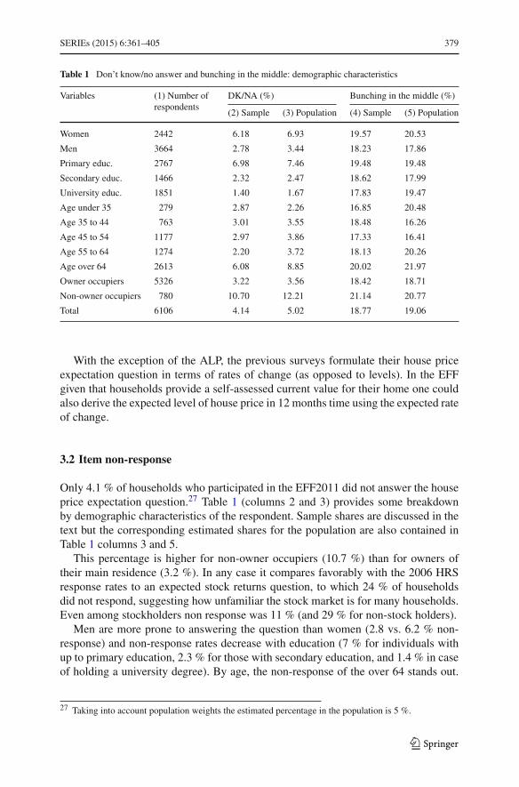
Only 4.1 % of households who participated in the EFF2011 did not answer the houseprice expectation question.27 Table 1 (columns 2 and 3) provides some breakdownby demographic characteristics of the respondent. Sample shares are discussed in thetext but the corresponding estimated shares for the population are also contained inTable 1 columns 3 and 5.

This percentage is higher for non-owner occupiers (10.7 %) than for owners oftheir main residence (3.2 %). In any case it compares favorably with the 2006 HRSresponse rates to an expected stock returns question, to which 24 % of householdsdid not respond, suggesting how unfamiliar the stock market is for many households.Even among stockholders non response was 11 % (and 29 % for non-stock holders).

Men are more prone to answering the question than women (2.8 vs. 6.2 % non-response) and non-response rates decrease with education (7 % for individuals withup to primary education, 2.3 % for those with secondary education, and 1.4 % in caseof holding a university degree). By age, the non-response of the over 64 stands out.

27 Taking into account population weights the estimated percentage in the population is 5 %.

123

380 SERIEs (2015) 6:361–405

Table 2 Observed answers and characteristics: multiple regressions

Variables (1) (2) (3) (4) (5)

dk/na + or − same Points toincrease (×10)

Points todrop (×10)

All points toone drop interval

Woman 0.025** −0.010 0.959 −1.785 −0.032**

Secondary educ. −0.010 0.019 −0.661 0.638 0.017

University educ. −0.005 0.052 −1.938 −2.218 −0.028

Age 35–44 0.001 −0.009 −1.148 6.966 0.053

Age 45–54 0.043*** 0.028 −0.694 −0.171 0.034

Age 55–64 0.034* 0.086* −1.906 −3.583 0.042

Age over 64 0.061*** 0.081* −3.105 −3.703 0.036

Blue collar 0.005 0.026 −0.223 −2.910 −0.018

Self-employed −0.008 0.021 −1.463 1.785 −0.015

Log (hh income) −0.020** 0.002 −0.461 2.608* 0.013

Wealth percentiles

25–50 −0.003 0.009 −0.512 −1.857 0.041

50–75 −0.024 0.041 0.034 −3.903 0.021

75–90 −0.005 0.017 0.265 −1.987 0.024

90–100 −0.010 0.002 −0.520 −0.845 −0.011

Bought main recently −0.004 0.010 2.858** −4.256 −0.008

Own other housing −0.004 −0.014 −0.402 2.609 0.064***

Constant 0.233** 0.142 11.323 27.260 −0.050

Observations 5326 5326 5326 5326 5326

t-statistics in parenthesesAll specifications include postal dummies and have been estimated taking into account population weightsand the five imputed datasets*** p < 0.01, ** p < 0.05, * p < 0.1

Table 2 (column 1) presents results from a multiple regression including income andwealth variables as well.

In the EFF I construct various measures to assess the amount of questions thehousehold has provided an answer for. Among others, I calculate the percentage ofmonetary questions that have been answered with a point value (as opposed to aninterval) as the ratio of exact answers to total questions posed to the households. Thecorrelation of this precise information ratio with not having answered the house priceexpectations question is −0.10 (−0.17 with a t-ratio of 8.2 in a simple regression).Not answering the house price expectation question also correlates significantly withnot having been able to provide an estimate of the current value of their home (0.10;0.05 with a t-ratio of 7.4 in a simple regression).28

28 Only homeowners are asked to provide an estimate of how much their house is worth.

123

SERIEs (2015) 6:361–405 381

3.3 Coherency analysis

Bunching in the middle of the scaleThe percentage of respondents placing all ten pointsin the middle-of-the-scale option is 18.8 %. For reference, in the 2006 HRS 23 % ofrespondents chose the middle of the scale to the question on survival probability toage 75 and 30 % chose it as a response to a question about the probability of stockmarket gains.29

There is certain heterogeneity by demographic groups (see Table 1, columns 4 and5). Among home-owners 18.4 % chose this answer while the share among non homeowners is 21.1 %. There is also some variation by education (varying from 19.5 %for respondents with no secondary education to 17.8 % in the ca.se of Universityeducated respondents). By gender there are some differences as well (18.2 % in thecase of men, 19.6 % for women). Differences by age are less noticeable (rangingfrom 16.8 % among the under 34–20 % among the over 64). In a multiple regression(see Table 2, column 2) only being aged over 64 has a significant (positive) effecton bunching. All in all these are small differences across groups, which is suggestiveof bunching driven by beliefs more than by ignorance, except may be for the olderrespondents.

The correlation between the constructed information ratio variable and choosingto put all ten points in the middle of the scale is not significant (0.004 and 0.01 witha t-ratio of 0.31 in a simple regression). Along the same lines, the correlation withnot being able to provide a value of their home is not significant either (−0.002 and−0.002 with a t-ratio of 0.13 in a simple regression).

The effects of demographic variables do not work in the same direction as in thecase of non-response and are much less significant in this case despite the sizeablenumber of such respondents (Table 2, column 2). This may indicate that there aredifferent factors at work. Namely, while a fraction of individuals giving all ten pointsto the approximately no house price change option may do so because they are unableto express beliefs about the future path of house prices there are others who stronglybelieve (i.e. put all ten points) that the price of their house will experience no changeover the next 12 months (see more details on epistemic uncertainty in Sect. 2.3). Theabsence of correlation with the information ratio and with not answering the currentvalue of their house points in this direction as well. Unfortunately, I cannot separatethe two types of answers because in the EFF the house price expectation question isnot followed by one trying to disentangle ignorance from genuine belief of no changein house prices.

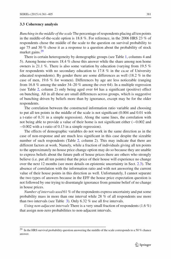
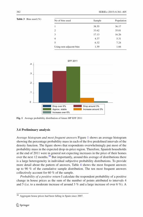
Number of intervals used 61% of the respondents express uncertainty and put someprobability mass in more than one interval while 28 % of all respondents use morethan two intervals (see Table 3). Only 6.32 % use all five intervals.

Using non-adjacent intervals There is a very small fraction of respondents (1.6 %)that assign non-zero probabilities to non-adjacent intervals.

29 In the HRS survival probability question answering the middle of the scale corresponds to a 50% chanceanswer.

123

382 SERIEs (2015) 6:361–405

Table 3 Bins used (%)No of bins used Sample Population

1 38.55 36.17

2 33.62 35.01

3 17.13 16.26

4 4.37 5.31

5 6.32 7.24

Using non-adjacent bins 1.59 1.66

0

.1

.2

.3

.4EFF 2011

Drop over 6% Drop around 3%Approx. stable Increase around 3%Increase over 6%

Fig. 1 Average probability distribution of future HP EFF 2011

3.4 Preliminary analysis

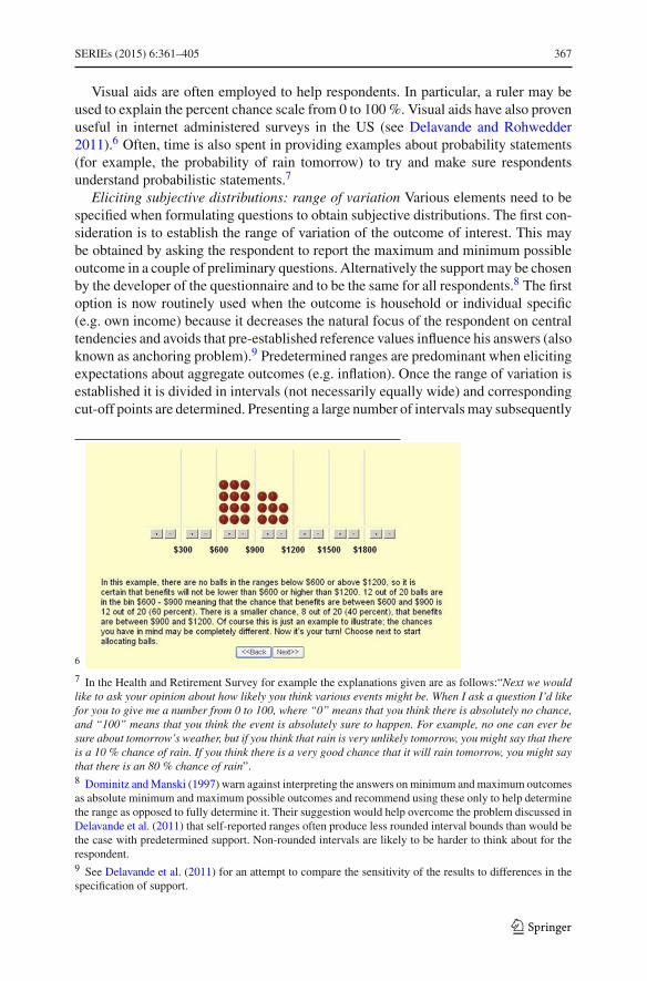
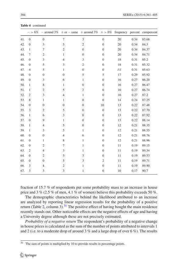
Average histogram and most frequent answers Figure 1 shows an average histogramshowing the percentage probability mass in each of the five predefined intervals of thedensity function. The figure shows that respondents overwhelmingly put most of theprobability mass in the expected drop-in-price region. Therefore, Spanish householdsat the end of 2011 were in general not expecting increases in the price of their homesover the next 12 months.30 But importantly, around this average of distributions thereis a large heterogeneity in individual subjective probability distributions. To providemore detail about the pattern of answers, Table 4 shows the most frequent answersup to 90 % of the cumulative sample distribution. The ten most frequent answerscollectively account for 60 % of the sample.

Probability of a positive return I calculate the respondent probability of a positivechange in house prices as the sum of the number of points attributed to intervals 4and 5 (i.e. to a moderate increase of around 3 % and a large increase of over 6 %). A

30 Aggregate house prices had been falling in Spain since 2007.

123

SERIEs (2015) 6:361–405 383

Table 4 Most frequent answers to probabilistic expectations of future house prices

− > 6% − around 3% + or − same + around 3% + > 6% Frequency Percent Cumpercent

1. 0 0 10 0 0 1146 19.58 19.58

2. 0 10 0 0 0 583 9.96 29.54

3. 10 0 0 0 0 558 9.53 39.7

4. 0 5 5 0 0 382 6.53 45.60

5. 5 5 0 0 0 323 5.52 51.12

6. 8 2 0 0 0 125 2.14 53.25

7. 0 3 7 0 0 116 1.98 55.24

8. 0 2 8 0 0 111 1.90 57.13

9. 6 4 0 0 0 91 1.55 58.69

10. 0 8 2 0 0 79 1.35 60.4

11. 3 7 0 0 0 79 1.35 61.39

12. 2 8 0 0 0 73 1.25 62.63

13. 0 0 5 5 0 73 1.25 63.88

14. 7 3 0 0 0 70 1.20 65.8

15. 0 6 4 0 0 70 1.20 66.27

16. 0 4 6 0 0 65 1.11 67.38

17. 0 7 3 0 0 64 1.9 68.48

18. 4 6 0 0 0 64 1.9 69.57

19. 2 6 2 0 0 57 0.97 70.55

20. 5 3 2 0 0 56 0.96 71.50

21. 4 4 2 0 0 55 0.94 72.44

22. 0 0 0 10 0 54 0.92 73.36

23. 3 5 2 0 0 52 0.89 74.25

24. 2 3 5 0 0 52 0.89 75.14

25. 2 5 3 0 0 51 0.87 76.1

26. 6 3 1 0 0 47 0.80 76.82

27. 2 4 4 0 0 36 0.62 77.43

28. 0 0 8 2 0 35 0.60 78.3

29. 3 3 4 0 0 32 0.55 78.58

30. 2 2 6 0 0 31 0.53 79.10

31. 0 1 9 0 0 31 0.53 79.63

32. 0 2 6 2 0 28 0.48 80.11

33. 4 3 3 0 0 27 0.46 80.57

34. 5 4 1 0 0 26 0.44 81.2

35. 9 1 0 0 0 26 0.44 81.46

36. 2 7 1 0 0 23 0.39 81.86

37. 3 4 3 0 0 23 0.39 82.25

38. 6 2 2 0 0 22 0.38 82.62

39. 3 6 1 0 0 21 0.36 82.98

40. 1 2 7 0 0 21 0.36 83.34

123

384 SERIEs (2015) 6:361–405

Table 4 continued

− > 6% − around 3% + or − same + around 3% + > 6% frequency percent cumpercent

41. 0 0 7 3 0 20 0.34 83.68

42. 0 3 5 2 0 20 0.34 84.3

43. 1 7 2 0 0 20 0.34 84.37

44. 7 2 1 0 0 20 0.34 84.71

45. 0 3 4 3 0 18 0.31 85.2

46. 0 5 3 2 0 18 0.31 85.32

47. 4 5 1 0 0 I S 0.31 85.63

48. 0 0 0 5 5 17 0.29 85.92

49. 0 3 6 1 0 16 0.27 86.20

50. 1 8 1 0 0 16 0.27 86.47

51. 1 2 5 2 0 16 0.27 86.74

52. 2 3 4 1 0 16 0.27 87.2

53. 8 1 1 0 0 14 0.24 87.25

54. 0 0 0 0 10 13 0.22 87.48

55. 3 2 5 0 0 13 0.22 87.70

56. 1 6 3 0 0 13 0.22 87.92

57. 0 9 1 0 0 13 0.22 88.14

58. 1 4 5 0 0 12 0.21 88.35

59. 1 3 5 1 0 12 0.21 88.55

60. 0 0 4 6 0 12 0.21 88.76

61. 0 1 8 1 0 12 0.21 88.96

62. 0 2 7 1 0 11 0.19 89.15

63. 2 4 3 1 0 11 0.19 89.34

64. 0 2 5 3 0 11 0.19 89.53

65. 0 0 5 3 2 11 0.19 89.71

66. 3 4 2 1 0 11 0.19 89.90

67. 3 3 3 1 0 10 0.17 90.7

fraction of 15.7 % of respondents put some probability mass to an increase in houseprice and 3 % (2.5 % of men, 4.1 % of women) believe this probability exceeds 50 %.

The demographic characteristics behind the likelihood attributed to an increaseare analyzed by reporting linear regression results for the probability of a positivereturn (Table 2, column 3).31 The positive effect of having bought the main residencerecently stands out. Other noticeable effects are the negative effects of age and havinga University degree although these are not precisely estimated.

Probability of a negative return The respondent’s probability of a negative changein house prices is calculated as the sum of the number of points attributed to intervals 1and 2 (i.e. to a moderate drop of around 3 % and a large drop of over 6 %). The results

31 The sum of points is multiplied by 10 to provide results in percentage points.

123

SERIEs (2015) 6:361–405 385

(Table 2, column 4) show no significant association of such beliefs with householdcharacteristics, except for a not very precise positive effect of household income.Negative house price expectations were therefore widespread across groups of thepopulation at the end of 2011.

No uncertainty 32.7 % of respondents believe the price of their homes will dropfor sure during 2012 (i.e. they distribute all points between intervals 1 and 2—largedrop over 6 %, moderate drop around 3 %). Over half of them (57.2 %) attribute allten points to one of the two price drop alternatives and hence answer without uncer-tainty. The results in the fifth column of Table 2 are an attempt to uncover demographicdifferences associatedwith these “no uncertainty” answers. The only significant differ-ence between these no-uncertainty respondents and the rest of respondents expecting adrop is gender and owning other housing.32 According to these results, women are lesslikely than men to give a 100 % probability to one of the two drop-in-price scenarios(and hence more likely than men to distribute the chances among the two alternatives).Additionally, households owning other housing aside from their main residence aremore likely to believe in a drop with no uncertainty about its magnitude.

Analyzing answerswithout uncertainty in the expected positive domain is not under-taken because it is hampered by the small number of observations.

3.5 Fitting subjective house price distributions

Calculating individual distributions As seen above, subjects are asked to distributeten points among five possible changes to the price of their homes over the next year. Iuse the subject responses to fit a saturated probability distribution for each respondent.This is useful because it facilitates the calculation of comparable measures of position,uncertainty, and quantiles for all individuals. Using a saturated distribution avoidsplacing restrictions on the form of the distribution relative to the information in thedata.

I assume that the probability distributions have a pre-specified support and a pre-specified neighborhood around zero for the no-change category. Having specifiedend-points and an interval around zero, to get a full cdf I connect the observed pointsusing straight lines so that the cdf is piece-wise linear and the density is flat withinsegments. This allows calculating all quantiles by linear extrapolation.

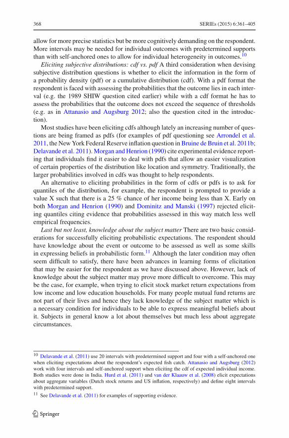
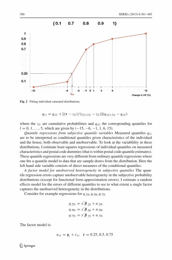
Figure 2 illustrates the estimation of the probability distribution for a respondenthaving distributed his ten points as follows: one point to a drop of more than 6 %,six points to a drop of around 3 %, one point to more or less the same, one point toan increase of around 3 % and one point to an increase larger than 6 %. The limitsof the support are defined to be −15 and +15 % and the interval around zero for thenon-change category to be between −1 and +1 %. To obtain the τ -quantile qτ i forsome τ ∈ (zli , z(l+1)i ) we use:

32 This analysis is conditioned on expecting a drop because I do not wish to mix determinants of certaintywith determinants of expecting a rise. Given the macroeconomic scenario, respondents that are certain ofa rise are few and probably with special characteristics. As for those putting all points to the “more or lessthe same“ option we have already analyzed their characteristics above.

123

386 SERIEs (2015) 6:361–405

Fig. 2 Fitting individual saturated distributions

qτ i = qzli + [(τ − zli )/(z(l+1)i − zli )](qz(l+1)i − qzli )

where the zli are cumulative probabilities and qzli the corresponding quantiles forl = 0, 1, . . ., 5, which are given by (−15, −6, −1, 1, 6, 15).

Quantile regressions from subjective quantile variables Measured quantiles qτ i

are to be interpreted as conditional quantiles given characteristics of the individualand the house, both observable and unobservable. To look at the variablility in thesedistributions, I estimate least squares regressions of individual quantiles on measuredcharacteristics and postal code dummies (that is within postal code quantile estimates).These quantile regressions are very different from ordinary quantile regressions whereone fits a quantile model to data that are sample draws from the distribution. Here theleft hand side variable consists of direct measures of the conditional quantiles.

A factor model for unobserved heterogeneity in subjective quantiles The quan-tile regression errors capture unobservable heterogeneity in the subjective probabilitydistributions (except for functional form approximation errors). I estimate a randomeffects model for the errors of different quantiles to see to what extent a single factorcaptures the unobserved heterogeneity in the distributions.

Consider for example regressions for q.25i,q.50i,q.75i

q.25i = x ′β .25 + u.25i

q.50i = x ′β .50 + u.50i

q.75i = x ′β .75 + u.75i

The factor model is:

uτ i = ηi + ετ i τ = 0.25, 0.5, 0.75

123

SERIEs (2015) 6:361–405 387

Table 5 Quantiles of subjective probability distributions of house prices (within postal code estimates)

Variables (1) (2) (3) (4) (5)

q10 q25 q50 q75 q90

Log (price/m2) 0.014 0.131 0.147 0.121 0.116

Age 45–64 0.608* 0.504* 0.379 0.150 −0.087

Age over 64 1.052*** 0.728** 0.432 0.100 −0.241

Blue collar 0.676** 0.604** 0.523** 0.406** 0.364**

Self-employed −0.563 −0.363 −0.327 −0.385 −0.412*

Secondary education 0.221 0.041 0.030 −0.025 −0.082

University education 0.595 0.506 0.382 0.268 0.137

Woman 0.228 0.367* 0.401** 0.323** 0.206

Own other housing −0.141 −0.225 −0.310 −0.331* −0.358**

Bought main residence recently 0.609 0.621* 0.578** 0.551** 0.508**

Log (household income) −0.103 −0.103 −0.125 −0.125 −0.131

Wealth percentiles 25–50 0.455 0.322 0.223 0.091 −0.181

Wealth percentiles 50–75 1.054** 0.765* 0.520 0.328 −0.010

Wealth percentiles 75–90 0.758 0.638 0.555 0.389 0.049

Wealth percentiles 90–100 0.258 0.246 0.212 0.139 −0.102

Constant −7.230** −5.811** −3.405* −1.279 0.643

Observations 5023 5023 5023 5023 5023

Adjusted R2 0.366 0.345 0.353 0.382 0.400

All specifications include postal dummies and have been estimated taking into account population weightsand the five imputed datasets*** p< 0.01, ** p < 0.05, * p < 0.1

I estimate the variance of the common factor ηi, the variances of the random errorsετ i and the factor loadings δτ subject to δ0.5 = 1 and the assumption that ηi and theετ i are mutually independent.

3.6 Relating heterogeneity in expectations to housing and householdcharacteristics

Individual density position measures and demographics I examine the associationbetween quantiles at various points of the estimated individual densities and demo-graphics, within postal codes.33 In particular I consider the individual median andthe 10th, 25th, 75th, and 90th percentiles as distributional measures for each respon-dent. Multiple regression results for those variables on demographics may be foundin Table 5.

The regression equations are of the form:

qτ i = Xiβτ + Ziγτ + uτ i

33 There are 1094 postal codes in our data, 212 of them have only one household and 71 have ten or more.

123

388 SERIEs (2015) 6:361–405

where Xi is a vector of household characteristics such as age, education, gender,income and wealth. Moreover, Zi is a vector of house characteristics, which includespostal code dummies, log (price/square meter) and in some cases also an indicator ofage of the house.

The results include the household estimated price (per square meter) of their home.Interestingly, the self-assessed house price of a household is not a significant predictorof the expected evolution of the price of its home conditional on postal code dummies(and the rest of included controls).

We observe lower expected declines in the lower part of the distribution as ageincreases. This relates to the finding by Malmendier and Nagel (2013) that experienceof older individuals draw on longer history of data when forming their expectationswhile expectations of younger ones are dominated by more recent data. In Spain in2011 the house price drops experienced since 2007 came after decades of rising houseprices.

Blue collar workers are associated with more optimistic expectations all over thedistribution while for the self-employed there is a negative shift in the upper part ofthe distribution. Households in the middle-upper part of the wealth distribution havetheir expectation distribution shifted upwards (more pronounced in the lower part).

Interestingly, there is a positive effect for those households who bought their mainresidence recently (in the last 6 years). Moreover, this effect is quite uniform acrossthe whole range of the distribution although more precise in the upper part of thedistribution. Recent buyers may be more reluctant to accept a prospect of no houseprice increases as compared to non-recent buyerswho have experienced sizeable houseprice returns. This effectmay also reflect reverse causality, that is, buyerswho expectedhigher house price changes than the rest were the ones who bought recently. Table 12presents results omitting this variable and the results are unchanged (columns 1 and2). The same result is obtained if instead a variable reflecting that the house was builtin the last 6 years is included. These could be taken as suggesting that the previousresult does not seem to be driven by reverse causality.

The results on gender stand up. Being a woman produces a positive shift that isparticularly noticeable at the median and at the top quartile. This is difficult to explainin terms of differences in information as one may do with occupation or age. It doesnot seem to be related to risk aversion either. Indeed, I have also included a measure ofrisk aversion available in the EFF but the results are unchanged (see Table 12 columns3 and 4).34

What these results say is that there is a difference by gender among the respondentsto the survey (controlling for postal code and other covariates), who aremeant to be the

34 We classify as risk lover those individuals answering options 1 or 2 to the following question:Which of the following statements do you feel best describes your household in terms of the amount offinancial risk you are willing to run when you make an investment?Take on a lot of risk in the expectation of obtaining a lot of profit 1Take on a reasonable amount of risk in the expectation of obtaining an above-normal profit 2Take on a medium level of risk in the expectation of obtaining an average profit 3You are not willing to take on financial risk 4Don’t know 98No answer 99

123

SERIEs (2015) 6:361–405 389

most knowledgeable about the household finances, as explained earlier.Whether thesedifferences would still hold for randomly selected individuals cannot be answered onthe current data.

To check the robustness of the gender result I estimated an Abadie and Imbens(2006) matching estimator of the gender average treatment effect which uses the con-trol variables in a non-parametric way. This produces similar results both inmagnitudeand significance. The same result is also found estimating the gender average treat-ment effect by weighting on the propensity score. This is at odds with the generallyaccepted finding that women tend to be less optimistic than men (see for exampleBalasuriya et al. 2010).

To further assess potential differences in asset valuations by gender we regressedself-assessed values of different assets reported in the EFF on the same demographicand socio-economic characteristics. The results in Table 13 show that women tend toprovide higher estimates for the value of their home compared to men but lower oneswhen it comes to value their financial assets.

An open research question in economic psychology is to what extent people’s priceperceptions and expectations are mediated by psychological variables like emotionsand attitudes (see for exampleRanyard et al. 2008). One hypothesis for further researchthat could explain our results would be that women positive affective feelings for theirhome (and its value) are stronger than for men and that these preferences affect thejudgment of men and women. For a detailed description and evidence see Slovic et al.(2001).

Are women more optimistic, or simply more realistic? A bold answer to this ques-tion can be based on the aggregate of counterfactual point predictions of house pricechanges across all households as if all were male respondents. Using the median as apoint forecast measure, the estimation results inform us that the counterfactual femaleaggregate is 0.4 percentage points higher than the corresponding male aggregate. Wecan now look at the actual aggregate house price change between 2011 and 2012 tofind out which one of the two genders was closer to the truth. The national houseprice change December 2011–December 2012 for second hand housing was around−10 %.35 The counterfactual aggregate male and female point forecasts are −3 and−2.6 %, respectively. Even if the position of the subjective probability distributionmay be affected by framing, the distance between actual and predicted changes is suf-ficiently large to conclude that women were more optimistic rather than more realisticby comparison with men.

Uncertainty and demographicsAs a first measure of individual forecast uncertaintyI consider the inter-quartile range. I also analyze the range given by the differencebetween the 90th and 10th percentiles. Heterogeneity in self-reported uncertainty isexamined in Table 6. A distinct effect on uncertainty in a multiple correlation contextis age. Older people express less uncertain expectations. Households in the middle-upper part of the wealth distribution are also less uncertain about their expectations.In line with other authors (see for example Bruine de Bruin et al. 2011a) I also find

35 It was −14 % according to the index from the National Statistics Office (INE) and −10 % according tothe Ministry of Public Works and online search-sites based on asking price data.

123

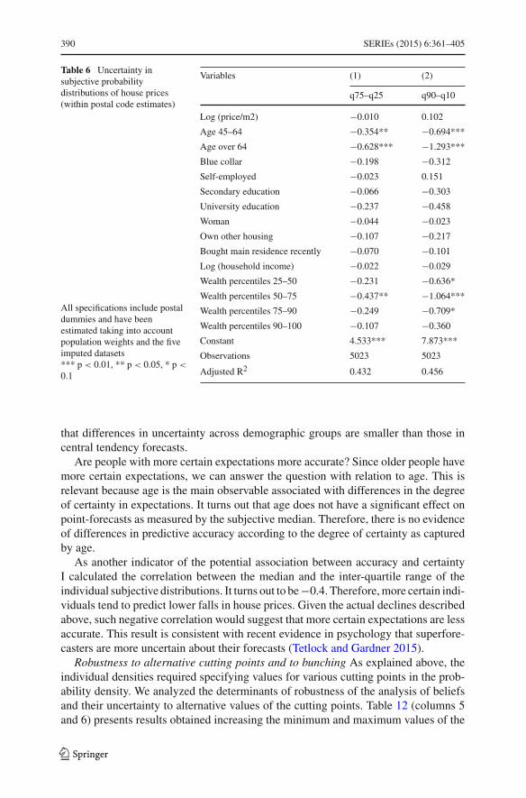
390 SERIEs (2015) 6:361–405

Table 6 Uncertainty insubjective probabilitydistributions of house prices(within postal code estimates)

All specifications include postaldummies and have beenestimated taking into accountpopulation weights and the fiveimputed datasets*** p < 0.01, ** p < 0.05, * p <

0.1

Variables (1) (2)

q75–q25 q90–q10

Log (price/m2) −0.010 0.102

Age 45–64 −0.354** −0.694***

Age over 64 −0.628*** −1.293***

Blue collar −0.198 −0.312

Self-employed −0.023 0.151

Secondary education −0.066 −0.303

University education −0.237 −0.458

Woman −0.044 −0.023

Own other housing −0.107 −0.217

Bought main residence recently −0.070 −0.101

Log (household income) −0.022 −0.029

Wealth percentiles 25–50 −0.231 −0.636*

Wealth percentiles 50–75 −0.437** −1.064***

Wealth percentiles 75–90 −0.249 −0.709*

Wealth percentiles 90–100 −0.107 −0.360

Constant 4.533*** 7.873***

Observations 5023 5023

Adjusted R2 0.432 0.456

that differences in uncertainty across demographic groups are smaller than those incentral tendency forecasts.

Are people with more certain expectations more accurate? Since older people havemore certain expectations, we can answer the question with relation to age. This isrelevant because age is the main observable associated with differences in the degreeof certainty in expectations. It turns out that age does not have a significant effect onpoint-forecasts as measured by the subjective median. Therefore, there is no evidenceof differences in predictive accuracy according to the degree of certainty as capturedby age.

As another indicator of the potential association between accuracy and certaintyI calculated the correlation between the median and the inter-quartile range of theindividual subjective distributions. It turns out to be−0.4. Therefore,more certain indi-viduals tend to predict lower falls in house prices. Given the actual declines describedabove, such negative correlation would suggest that more certain expectations are lessaccurate. This result is consistent with recent evidence in psychology that superfore-casters are more uncertain about their forecasts (Tetlock and Gardner 2015).

Robustness to alternative cutting points and to bunching As explained above, theindividual densities required specifying values for various cutting points in the prob-ability density. We analyzed the determinants of robustness of the analysis of beliefsand their uncertainty to alternative values of the cutting points. Table 12 (columns 5and 6) presents results obtained increasing the minimum and maximum values of the

123

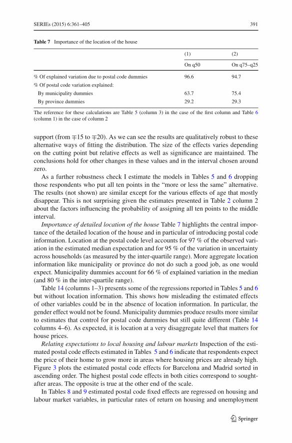
SERIEs (2015) 6:361–405 391

Table 7 Importance of the location of the house

(1) (2)

On q50 On q75–q25

% Of explained variation due to postal code dummies 96.6 94.7

% Of postal code variation explained:

By municipality dummies 63.7 75.4

By province dummies 29.2 29.3

The reference for these calculations are Table 5 (column 3) in the case of the first column and Table 6(column 1) in the case of column 2

support (from ∓15 to ∓20). As we can see the results are qualitatively robust to thesealternative ways of fitting the distribution. The size of the effects varies dependingon the cutting point but relative effects as well as significance are maintained. Theconclusions hold for other changes in these values and in the interval chosen aroundzero.

As a further robustness check I estimate the models in Tables 5 and 6 droppingthose respondents who put all ten points in the “more or less the same” alternative.The results (not shown) are similar except for the various effects of age that mostlydisappear. This is not surprising given the estimates presented in Table 2 column 2about the factors influencing the probability of assigning all ten points to the middleinterval.

Importance of detailed location of the house Table 7 highlights the central impor-tance of the detailed location of the house and in particular of introducing postal codeinformation. Location at the postal code level accounts for 97 % of the observed vari-ation in the estimated median expectation and for 95 % of the variation in uncertaintyacross households (as measured by the inter-quartile range). More aggregate locationinformation like municipality or province do not do such a good job, as one wouldexpect. Municipality dummies account for 66 % of explained variation in the median(and 80 % in the inter-quartile range).

Table 14 (columns 1–3) presents some of the regressions reported in Tables 5 and 6but without location information. This shows how misleading the estimated effectsof other variables could be in the absence of location information. In particular, thegender effect would not be found. Municipality dummies produce results more similarto estimates that control for postal code dummies but still quite different (Table 14columns 4–6). As expected, it is location at a very disaggregate level that matters forhouse prices.

Relating expectations to local housing and labour markets Inspection of the esti-mated postal code effects estimated in Tables 5 and 6 indicate that respondents expectthe price of their home to grow more in areas where housing prices are already high.Figure 3 plots the estimated postal code effects for Barcelona and Madrid sorted inascending order. The highest postal code effects in both cities correspond to sought-after areas. The opposite is true at the other end of the scale.

In Tables 8 and 9 estimated postal code fixed effects are regressed on housing andlabour market variables, in particular rates of return on housing and unemployment

123

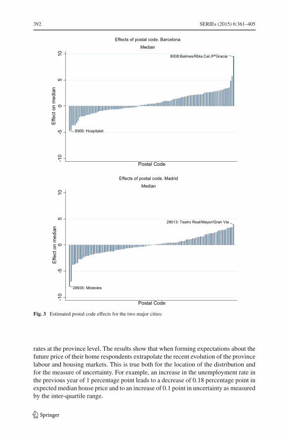
392 SERIEs (2015) 6:361–405

8906: Hospitalet

8008:Balmes/Rbla.Cat./PºGracia-1

0-5

05

10E

ffect

on

med

ian

Postal Code

Median

Effects of postal code. Barcelona

28013: Teatro Real/Mayor/Gran Via

28935: Móstoles

-10

-50

510

Effe

ct o

n m

edia

n

Postal Code

Median

Effects of postal code. Madrid

Fig. 3 Estimated postal code effects for the two major cities:

rates at the province level. The results show that when forming expectations about thefuture price of their home respondents extrapolate the recent evolution of the provincelabour and housing markets. This is true both for the location of the distribution andfor the measure of uncertainty. For example, an increase in the unemployment rate inthe previous year of 1 percentage point leads to a decrease of 0.18 percentage point inexpectedmedian house price and to an increase of 0.1 point in uncertainty as measuredby the inter-quartile range.

123

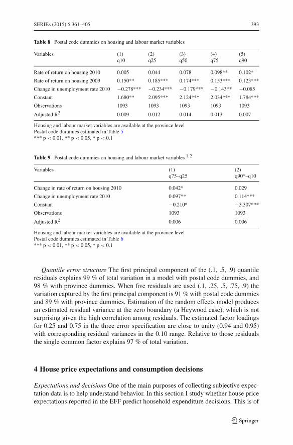
SERIEs (2015) 6:361–405 393

Table 8 Postal code dummies on housing and labour market variables

Variables (1) (2) (3) (4) (5)q10 q25 q50 q75 q90

Rate of return on housing 2010 0.005 0.044 0.078 0.098** 0.102*

Rate of return on housing 2009 0.150** 0.185*** 0.174*** 0.153*** 0.123***

Change in unemployment rate 2010 −0.278*** −0.234*** −0.179*** −0.143** −0.085

Constant 1.680** 2.095*** 2.124*** 2.034*** 1.784***

Observations 1093 1093 1093 1093 1093

Adjusted R2 0.009 0.012 0.014 0.013 0.007

Housing and labour market variables are available at the province levelPostal code dummies estimated in Table 5*** p < 0.01, ** p < 0.05, * p < 0.1

Table 9 Postal code dummies on housing and labour market variables 1,2

Variables (1) (2)q75–q25 q90*–q10

Change in rate of return on housing 2010 0.042* 0.029

Change in unemployment rate 2010 0.097** 0.114***

Constant −0.210* −3.307***

Observations 1093 1093

Adjusted R2 0.006 0.006

Housing and labour market variables are available at the province levelPostal code dummies estimated in Table 6*** p < 0.01, ** p < 0.05, * p < 0.1

Quantile error structure The first principal component of the (.1, .5, .9) quantileresiduals explains 99 % of total variation in a model with postal code dummies, and98 % with province dummies. When five residuals are used (.1, .25, .5, .75, .9) thevariation captured by the first principal component is 91 % with postal code dummiesand 89 % with province dummies. Estimation of the random effects model producesan estimated residual variance at the zero boundary (a Heywood case), which is notsurprising given the high correlation among residuals. The estimated factor loadingsfor 0.25 and 0.75 in the three error specification are close to unity (0.94 and 0.95)with corresponding residual variances in the 0.10 range. Relative to those residualsthe single common factor explains 97 % of total variation.

4 House price expectations and consumption decisions

Expectations and decisions One of the main purposes of collecting subjective expec-tation data is to help understand behavior. In this section I study whether house priceexpectations reported in the EFF predict household expenditure decisions. This is of

123

394 SERIEs (2015) 6:361–405

substantial interest in its own right and also a further step in the validation of theinformation collected.

Therewere large unexpected shocks to house price expectations in Spain after 2007.The percentage of households buying second housing decreased dramatically sincethe bursting of the housing bubble. In the three year period between the 2002 and the2005 EFFs, 5.2 % of households bought a second house (an average of over 1.7 %a year) while this percentage was only 0.6 % for 2011. Also according to EFF data,9.4%of the Spanish households bought a car in 2011. However, among the householdswho are very pessimistic about the future price of their house (i.e. those assigning allten points to the over 6 % drop scenario) only 4.5 % did so.36 In this section I useinformation on expenditure outcomes on various items available in the EFF to see ifhouse price expectations are predictive of purchase and expenditure decisions once arich set of controls are taken into account.

Expenditure and purchases in the EFF In the EFF households provide informationon whether they bought a car in the last 12 months and the price paid for those whodid. The same information is collected about other big ticket items (furniture, washingmachines etc) as a whole. Amounts spent on food at home and outside as well as onother non-durables are also collected.

The EFF provides detailed information on purchases of secondary housing (forhouseholds owning their main residence). Housing purchases are both consumptionand investment decisions. Bover (2010) provides evidence that aggregate predictedreturns on housing have a large positive effect on the hazard of purchasing a house.However, aggregate returns are probably masking different individual expectationsconcerning future house prices, both in terms of differences in household character-istics and in terms of differences in house specific attributes like location. I thereforeexplore if individual household expectations about house prices help predict the prob-ability of purchasing a house and, in case of purchase, the amount spent on it.

A word about the timing of subjective expectations and expenditure outcomes.Ideally, the interest is in how expectations held at t about the future influence decisionsat t . The expectation data correspond to beliefs held at the time of the interview, whilethe expenditure data refer to purchases during the last 12 months, which is a goodtiming approximation, specially for durables.

Empirical model First, probit estimates are presented for the probability of (1)buying secondary housing, (2) buying a car, and (3) buying other big ticket items (seeTable 10). To analyze expenditure I present tobit estimates for the amounts spent on(1) other housing, (2) cars, and (3) other big ticket items, and multivariate regressionsfor the amount spent on (4) food and other non durables (see Table 11a). As is well-known, tobit estimates rely on the assumption that the same relationship holds bothfor the decision to purchase and for the amount spent. To check how restrictive thisassumption is here the implied tobit estimates for the various purchase probabilitiesare also be provided (see Table 11b) and compared with the probit estimates.

36 At the end of 2011 23.3 % of households expected a large decrease (over 6 %) in the price of their homeover the next 12 months. Among those, 30.7 % expected this large drop without uncertainty that is 7.2 %of the population of households.

123

SERIEs (2015) 6:361–405 395

Table10

Effectsof

housepriceexpectations

onaverageprob

abilitie

sof

purchase

(atv

arious

pointsof

thewealth

distributio

n;prob

itestim

ates)

Other

housing

Car

purchase

Other

bigticketitems

Mem

o:%

ofho

useholds

buying

0.57

9.42

41.99

(1)

(2)

(3)

(4)

(5)

(6)

Expectatio

nvariablesa

Fullsample

With

inpostal

codes

Fullsample

With

inpostal

codes

Fullsample

With

inpostal

codes

Weigh

tsNoweigh

tsWeigh

tsNoweigh

tsWeigh

tsNoweigh

ts

Large

certaindrop

inHPb

Atm

ediannetw

ealth

−0.826

**−4

.06

−4.46*

*−1

1.7*

**2.80

−7.26*

*

At8

0thpercentileof

netw

ealth

−1.24*

**−4

.31

−2.83

−11.3*

**2.07

−6.46*

*

Uncertainty

inHPc

Atm

ediannetw

ealth

−0.629

*−5

.88*

*2.67

*0.29

68.09

***

0.46

1

At8

0thpercentileof

netw

ealth

−0.803

**−8

.27*

**2.64

−0.334

12.5**

*1.59

Incomehigh

erthan

currentd

−0.145

11.8*

2.14

1.56

0.72

44.95

**

Incomelower

than

current

0.65

6−4

.43

1.77

1.83

−0.007

−1.91

Observatio

nse

5019

381

5019

2158

5019

4189

***p

<0.01

,**p

<0.05

,*p

<0.1

aCon

trol

variablesinclud

e:interactions

ofexpectationdu

mmieswith

lognetw

ealth

,gender,agebrackets,n

umberof

person

sin

theho

useholddu

mmies,child

rendummy,

coup

ledu

mmy,labo

urstatus

dummiesforrespon

dent

andpartner(ifany),p

ositive

andnegativ

eincomeshocks

dummiesandin

columns

1,3,

5and7mun

icipality

size

dummiesinsteadof

postalcode

dummies

bLarge

certaindrop

=1ifrespon

dent

assign

sallten

pointsto

“large

drop

(moretan6%)”

Large

certaindrop

=0ifrespon

dent

assign

sallten

pointsto

anyotherof

the4otherop

tions

cUncertainty

=1ifrespon

dent

assign

spo

intsto

morethan

oneop

tion

Uncertainty

=0ifrespon

dent

assign

stenpo

intsto

anyof

the4op

tions

differentfrom

“large

drop

(>6%)”

dIncomehigh

er(low

er)than

current=

1iffuture

expected

incomehigh

er(low

er)than

current,0otherw

ise

eSamplesizesvary

slightly

across

imputatio

ns.T

henumbersshow

ncorrespond

tothesm

allersamplesize

fProbabilitiesareshow

nin

percentage

term

s

123

396 SERIEs (2015) 6:361–405

Table11

Effectsof

housepriceexpectations

on(a)expend

ituresand(b)averageprob

abilitie

sof

purchase

from

tobitm

odel(atv

arious

pointsof

thewealth

distributio

n)

Other

Hou

sing

(Tob

it)Car

purchase

(Tob

it)Other

bigtic

ketitems(Tob

it)Fo

odandotherno

n-du

rables

(log

)

Expectatio

nvariablesa

(1)

(2)

(3)

(4)

(5)

(6)

(7)

(8)

With

inpostalcodesb

With

inpostalcodes

With

inpostalcodes

With

inpostalcodes

(a)

Large

certaindrop

inHPc

Atm

ediannetw

ealth

−876

,501

**−8

11,159

***

−11,58

0*−1

2,97

5**

260.1

−705

.20.03

190.04

02

At8

0thpercentileof

net

wealth

−676

,699

**−4

83,728

***

−499

5−5

105

652.0

−667

.80.04

310.05

66

Uncertainty

inHPd

Atm

ediannetw

ealth

−229

,984

**−5

07,576

***

3761

1871

646.9

69.92

0.02

550.01

02

At8

0thpercentileof

net

wealth

−180

,981

**−3

80,539

***

4063

2793

1497

**62

6.2

0.04

86*

0.02

95

Incomehigh

erthan

currente

−47,60

750

,864

2694

−843

.1−3

15.5

222.3

0.07

69**

*−0

.106

***

Incomelower

than

current

155,66

4*−1

43,444

2137

2104

−282

.4−6

69.6

−0.014

00.00

542

Observatio

nsf

5019

5019

5019

5019

5019

5019

5019

5019

Ofwhich

uncensored

g40

4041

241

219

5919

5950

1950

19

123

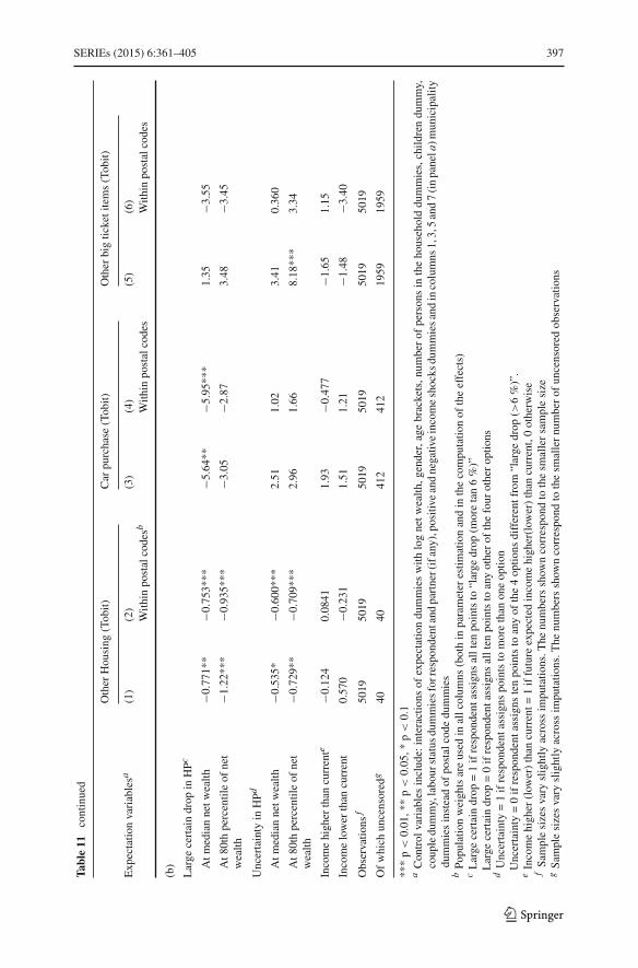
SERIEs (2015) 6:361–405 397

Table11

continued

Other

Housing

(Tobit)

Car

purchase

(Tobit)

Other

bigticketitems(Tobit)

Expectatio

nvariablesa

(1)

(2)

(3)

(4)

(5)

(6)

With

inpostalcodesb

With

inpostalcodes

With

inpostalcodes

(b)

Large

certaindrop

inHPc

Atm

ediannetw

ealth

−0.771

**−0

.753

***

−5.64*

*−5

.95*

**1.35

−3.55

At8

0thpercentileof

net

wealth

−1.22*

**−0

.935

***

−3.05

−2.87

3.48

−3.45

Uncertainty

inHPd

Atm

ediannetw

ealth

−0.535

*−0

.600

***

2.51

1.02

3.41

0.36

0

At8

0thpercentileof

net

wealth

−0.729

**−0

.709

***

2.96

1.66

8.18

***

3.34

Incomehigh

erthan

currente

−0.124

0.08

411.93

−0.477

−1.65

1.15

Incomelower

than

current

0.57

0−0

.231

1.51

1.21

−1.48

−3.40

Observatio

nsf

5019

5019

5019

5019

5019

5019

Ofwhich

uncensored

g40

4041

241

219

5919

59

***p

<0.01

,**p

<0.05

,*p

<0.1

aCon

trol

variablesinclud

e:interactions

ofexpectationdu

mmieswith

lognetw

ealth

,gender,agebrackets,n

umberof

person

sin

theho

useholddu

mmies,child

rendummy,

coup

ledu

mmy,labo

urstatus

dummiesforrespo

ndentand

partner(ifany),positive

andnegativ

eincomeshocks

dummiesandincolumns

1,3,5and7(inpanela)m

unicipality

dummiesinsteadof

postalcode

dummies

bPo

pulatio

nweightsareused

inallcolum

ns(bothin

parameter

estim

ationandin

thecomputatio

nof

theeffects)

cLarge

certaindrop

=1ifrespon

dent

assign

sallten

pointsto

“large

drop

(moretan6%)”

Large

certaindrop

=0ifrespon

dent

assign

sallten

pointsto

anyotherof

thefour

otherop

tions

dUncertainty

=1ifrespon

dent

assign

spo

intsto

morethan

oneop

tion

Uncertainty

=0ifrespon

dent

assign

stenpo

intsto

anyof

the4op

tions

differentfrom

“large

drop

(>6%)”.

eIncomehigh

er(low

er)than

current=

1iffuture

expected

incomehigh

er(low

er)than

current,0otherw

ise

fSamplesizesvary

slightly

across

imputatio

ns.T

henumbersshow

ncorrespond

tothesm

allersamplesize

gSa

mplesizesvary

slightly

across

impu

tatio

ns.T

henu

mbersshow

ncorrespo

ndto

thesm

allernu

mberof

uncensored

observations

123

398 SERIEs (2015) 6:361–405

In the empirical models I include two variables measuring household beliefs aboutfuture house prices. To reflect the location of those expectations, a 0/1 dummy isdefined taking the value 1 for people expecting a large certain drop with certainty(i.e. people who assign all ten points to the option “more than 6 %” drop). To captureuncertainty about the expectation location another 0/1 dummy is defined taking thevalue 1 for respondents assigning points to more than one option. Note that theseindicators are constructed directly from the household responses, and not from fittedindividual probability distributions.

A potential concern of reverse causality is that the uncertainty about the futureprice of the main residence may be reduced by investment in information associatedwith the purchase of other housing. However, the results in Table 6 indicate a lack ofassociation between uncertainty and having bought themain residence recently, whichsuggests that endogenous reductions in uncertainty may not be very important.

Importantly, I amable to control for expectations about future household incomeandhence identify house price expectations net of income expectations. In the EFF2011expectations about future household income are collected albeit in a qualitative way.Households are asked whether, compared to their current income, they believe theirincome in the future will be higher, lower, or approximately the same. Two indicatorsare constructed containing such that information.37

Additionally, the occurrence of positive or negative income shocks is controlled forby exploiting the information provided by a question in the EFF on whether currenthousehold income is higher than usual, lower than usual or as usual.

Other variables included in the estimated models are: log net household wealth andits interactions with the house price expectations dummies, respondent gender, age(six interval variables), number of persons in the household (six 0/1 dummies), coupledummy, children dummy, labour status dummies for respondent (four categories) andpartner (if any).

Regarding location variables two sets of results are presented: controlling formunic-ipality size (seven categories) or by postal code. However, probit estimates controllingfor postal codes rely on a significantly reduced number of observations because of therequirement of observing households who buy and households who do not buy atpostal code level (columns 2, 4, 6 in Table 10). Those results therefore cannot be takenas representative of the population of households. This is not the case for the tobitestimates in Table 11a, b.

ResultsThe results inTable 10 (column1) show that themost pessimistic householdshave a significantly lower probability of buying a house than the rest. The reduction inprobability is of 0.8 percentage point at the median level of wealth but higher (1.24 pp)at the 80th wealth percentile. Uncertainty about the evolution of future house prices isalso associated with reductions in the probability of buying a house. The magnitudeof this reduction is 0.63 pp at the median and 0.8 at the 80th percentile. Larger effectsat the top of the wealth distribution appear sensible as those are the households mostprone to buying second housing.

37 Starting from the 2014 wave the EFF includes a question on probabilistic expectations about future totalhousehold income.

123

SERIEs (2015) 6:361–405 399

Expecting a large drop in house prices is also associated with a 4.5 pp smallerprobability of buying a car at the median level of wealth but not for wealthier house-holds. However, uncertain expectations are positively correlated with the probabilityof buying a car and, mostly, with other big ticket items. These results could reflectsome substitution effects.

Table 11a shows the estimates for the various expenditures. Again, the larger andmost significant effects are the reduction in the amounts spent when buying secondhousing for households expecting a large drop in the price of their house or for thosebeing uncertain about the evolution of the value of their home. For these householdsthe amounts spentwhen buying a car are also significantly lower (−13,000e atmedianwealth). These conclusions hold when postal code dummies are included.

Similarly to the results on purchase probabilities, there seem to be some evidenceof some substitution effects for expenditures on other big ticket items and on food andother non-durables among wealthy households uncertain about future house prices.However, these results do not hold when controlling for postal code.

Finally, Table 11b reports the probabilities of purchase of the various items obtainedfrom the tobit model. These are very much in line with those obtained with the probitmodel (see Table 10). Furthermore, in this case estimates of the probabilities control-ling for postal code can be obtained for the whole sample and confirm the results incolumns 1, 3, and 5 of Tables 10 and 11b.

5 Conclusions

Household predictive probability distributions play an important role in explainingbehavior in many contexts. Not only the location of these distributions but alsothe uncertainty with which households hold their beliefs is relevant. It is thereforeimportant to have at our disposal measures of such probabilistic expectations directlycollected from households.

In this paper I have first reviewed recent work about expectations elicited in house-hold surveys. In particular, I have described relevant implementation specificities aswell as reviewed various uses of subjective probabilistic expectation questions.

Second, I have analyzed the answers to a question recently introduced in the EFFon probabilistic house price expectations. This analysis shows that asking such type ofquestions to Spanish households is feasible (as long as respondents are familiar withthe subject matter), as shown by the high response rate and the results of a coherencyanalysis.

The results show significant heterogeneity in house price expectations acrossrespondents. Heterogeneity is found to be significant both for the location of suchexpectations as well as for the amount of uncertainty around them. I find that womenand blue collar workers are more optimistic about the evolution of house prices for2012, and older respondents are more certain.

123

400 SERIEs (2015) 6:361–405

The results also provide valuable information about heterogeneity in the housingmarket. Location of the house at the postal code level is shown to explain most ofthe observed heterogeneity in expectations. Moreover, past returns to housing andunemployment rates are found to be strong determinants of the estimated effects oflocation.

Furthermore, the results show that in the absence of controlling for detailed locationinformation about the house the estimated effects of demographic characteristics onhouse price expectations are biased and misleading.

I also exploit the availability of information about various durable and non-durableexpenditures in the EFF and present some novel findings about the association betweenhouse price probabilistic expectations (location and uncertainty) and various durableexpenditures. The results show that households holding pessimistic expectations havesignificantly lower probabilities of buying a house and of buying a car. Moreover, theamounts spent on those items by buyers are also smaller than in the absence of suchnegative expectations. However, I find no association between house price expecta-tions and expenditure on other big ticket items, nor on food and other nondurableexpenditure.

Finally, greater uncertainty in house price expectations is associated with a lowerprobability of buying a secondary house (as well as with smaller amounts spent) butnot with the purchase or the amount spent in other goods.

Open Access This article is distributed under the terms of the Creative Commons Attribution 4.0 Interna-tional License (http://creativecommons.org/licenses/by/4.0/), which permits unrestricted use, distribution,and reproduction in any medium, provided you give appropriate credit to the original author(s) and thesource, provide a link to the Creative Commons license, and indicate if changes were made.

6 Appendix

See Tables 12, 13 and 14.

123

SERIEs (2015) 6:361–405 401

Table12

Various

robustness

checks

(1)

(2)

(3)

(4)

(5)

(6)

Variables

Norecent

buyervariable

Riskaversion

Wider

support

q50

q75-q2

5q5

0q7

5-q2

5q5

0q7

5-q2

5

Log

(price/m

2)0.18

2−0

.014

0.14

5−0

.012

0.17

9−0

.045

Age

45–6

40.32

5−0

.347

**0.32

6−0

.301

*0.42

4−0

.491

**

Age

over

640.37

80.62

1***

0.32

10.51

4***

0.49

30.79

2***

Bluecolla

r0.53

0**

−0.199

0.55

4***

−0.227

*0.63

9***

−0.327

*

Self-employed

−0.340

−0.021

−0.362

0.00

7−0

.379

0.03

7

Second

aryeducation

0.05

0−0

.068

0.02

2−0

.055

0.01

5−0

.052

University

education

0.417

−0.242

0.35

3−0

.197

0.47

9−0

.369

Wom

an0.38

1**

−0.041

0.42

2**

−0.050

0.50

0**

−0.141

Ownotherhousing

−0.295

−0.109

−0.273

−0.153

−0.410

*−0

.054

Bou

ghtm

ainresidencerecently

––

0.50

1*0.00

40.67

7**

−0.176

Risklover

––

−0.189

0.67

6–

–

Log

(hou

seho

ldincome)

−0.113

−0.024

−0.133

−0.008

−0.146

−0.030

Wealth

percentiles

25–5

00.12

9−0

.220

0.21

2−0

.205

0.26

1−0

.364

Wealth

percentiles

50–7

50.41

0−0

.423

**0.52

2−0

.430

**0.62

3*−0

.635

**

Wealth

percentiles

75–9

00.43

0−0

.233

0.57

4−0

.265

0.72

0*−0

.457

Wealth

percentiles

90–1

000.09

0−0

.092

0.25

2−0

.143

0.31

0−0

.167

Con

stant

−3.392

*4.53

1***

−3.256

4.33

8***

−3.860

*5.80

1***

Observatio

ns50

2350

2350

0450

0450

2350

23

AdjustedR2

0.35

10.43

20.35

40.43

70.35

90.40

7

***p

<0.01

,**p

<0.05

,*p

<0.1

Allspecificatio

nsincludepostaldummiesandhave

been

estim

ated

taking

into

accountp

opulationweightsandthefiv

eim

puteddatasets

123

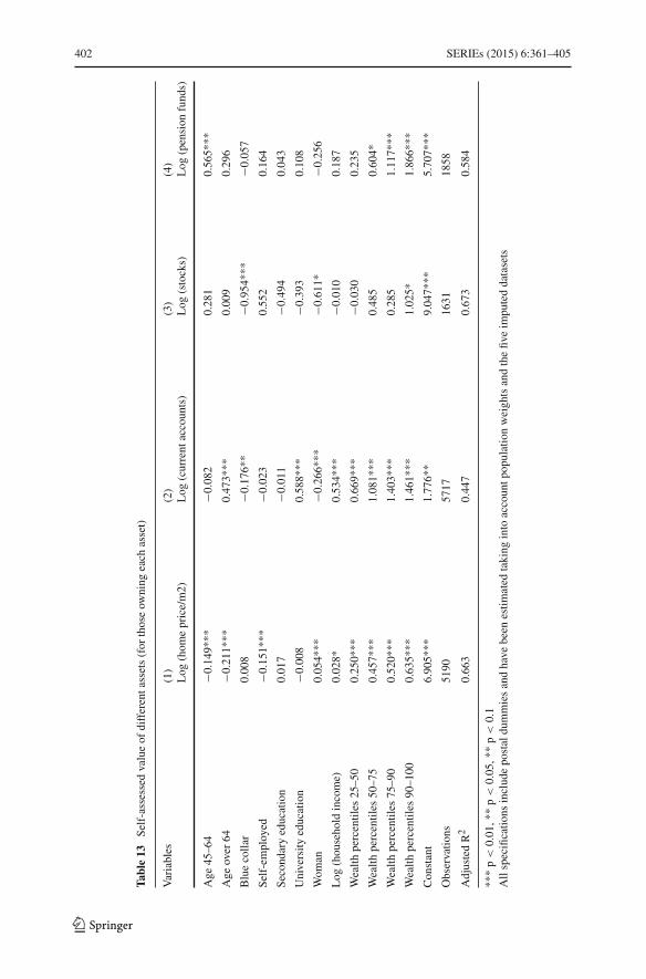
402 SERIEs (2015) 6:361–405

Table13

Self-assessedvalueof

differentassets(for

thoseow

ning

each

asset)

Variables

(1)

(2)

(3)

(4)

Log

(hom

eprice/m2)

Log

(current

accoun

ts)

Log

(stocks)

Log

(pension

fund

s)

Age

45–6

4−0

.149

***

−0.082

0.28

10.56

5***

Age

over

64−0

.211

***

0.47

3***

0.00

90.29

6

Bluecolla

r0.00

8−0

.176

**−0

.954

***

−0.057

Self-employed

−0.151

***

−0.023

0.55

20.16

4

Second

aryeducation

0.01

7−0

.011

−0.494

0.04

3

University

education

−0.008

0.58

8***

−0.393

0.10

8

Wom

an0.05

4***

−0.266

***

−0.611

*−0

.256

Log

(hou

seho

ldincome)

0.02

8*0.53

4***

−0.010

0.18

7

Wealth

percentiles

25–5

00.25

0***

0.66

9***

−0.030

0.23

5

Wealth

percentiles

50–7

50.45

7***

1.08

1***

0.48

50.60

4*

Wealth

percentiles

75–9

00.52

0***

1.40

3***

0.28

51.11

7***

Wealth

percentiles

90–1

000.63

5***

1.46

1***

1.02

5*1.86

6***

Con

stant

6.90

5***

1.77

6**

9.04

7***

5.70

7***

Observatio

ns51

9057

1716

3118

58

AdjustedR2

0.66

30.44

70.67

30.58

4

***p

<0.01

,**p

<0.05

,**p

<0.1

Allspecificatio

nsincludepostaldummiesandhave

been

estim

ated

taking

into

accountp

opulationweightsandthefiv

eim

puteddatasets

123

SERIEs (2015) 6:361–405 403

Table14

Somequ

antilemeasuresof

subjectiv

eprob

ability

distributio

nsof

houseprices:(1)

nolocatio

ninform

ation,

(2)mun

icipality

dummies

Variables

(1)

(2)

(3)

(4)

(5)

(6)

Nolocatio

ninform

ation

Municipality

dummies

q25

q50

q75-q2

5q2

5q5

0q7

5-q2

5

Log

(price/m

2)−0

.237

−0.074

0.25

6***

−0.142

−0.019

0.14

8

Age

45–6

40.07

90.11

3−0

.061

0.28

10.27

2−0

.157

Age

over

640.39

80.11

4−0

.621

***

0.64

5**

0.48

1*−0

.473

***

Bluecolla

r0.42

30.38

7*−0

.118

0.46

4*0.41

2*−0

.188

Self-employed

−0.395

−0.444

−0.171

−0.315

−0.217

0.03

2

Second

aryeducation

−0.295

−0.286

−0.009

−0.124

−0.102

−0.028

University

education

0.42

10.34

5−0

.199

0.45

40.39

6−0

.177

Wom

an0.29

40.22

6−0

.161

0.26

90.31

3*−0

.001

Ownotherhousing

−0.102

−0.236

−0.174

−0.123

−0.217

−0.116

Bou

ghtm

ainresidencerecently

0.87

8**

0.60

5*−0

.437

**0.75

3**

0.63

9**

−0.166

Log

(hou

seho

ldincome)

−0.071

−0.144

−0.108

−0.121

−0.132

−0.021

Wealth

percentiles

25–5

00.63

50.22

1−0

.650

***

0.65

2*0.31

6−0

.471

**

Wealth

percentiles

50–7

51.02

4**

0.47

4−0

.833

***

1.05

6***

0.58

3*−0

.642

***

Wealth

percentiles

75–9

00.95

4**

0.42

5− 0

.764

***

0.89

1**

0.47

4−0

.531

**

Wealth

percentiles

90–1

000.71

90.30

4−0

.537

*0.54

60.17

8−0

.396

Con

stant

−3.939

*−1

.508

4.31

4***

0.72

30.77

70.73

6

Observatio

ns50

2350

2350

2350

2350

2350

23

AdjustedR2

0.01

160.00

988

0.02

180.20

80.20

90.31

8

Allspecificatio

nshave

been

estim

ated

taking

into

accoun

tpop

ulationweigh

tsandthefiv

eim

puteddatasets.C

olum

ns1to

3includ

eno

locatio

ndu

mmiesandcolumns

4to

6includ

emun

icipality

dummies

***p

<0.01

,**p

<0.05

,*p

<0.1

123

404 SERIEs (2015) 6:361–405

References

Abadie A, Imbens G (2006) Large sample properties of matching estimators for average treatment effects.Econometrica 74:235–267

Armantier O, Bruine de Bruin W, Potter S, Topa G, van der KlaauwW, Zafar B (2013) Measuring inflationexpectations. Annu Rev Econ 5(1):273–301

Arrondel L, Calvo-Pardo H, Tas D (2011) Subjective stock market expectations, information and stockmarket participation: evidence from France (unpublished manuscript)

Attanasio O (2009) Expectations and perceptions in developing countries: their measurement and their use.Am Econ Rev Papers Proc 99:87–92

Attanasio O, Augsburg B (2012) Subjective expectations and income process in rural India (unpublishedmanuscript)

Balasuriya J, Muradoglu G, Ayton P (2010) Optimism and portfolio choice (unpublished manuscript)Benítez-Silva H, Dwyer DS, Gayle W, Muench TJ (2008) Expectations in micro data: rationality revisited.

Empir Econ 34(2):381–416Blanchflower DG, MacCoille C (2009) The formation of inflation expectations: an empirical analysis for

the UK, NBER Working Paper No 15388Bover O (2010) Housing purchases and the dynamics of housing wealth, CEPR Discussion Paper No 8128,

Banco de España Working Paper 1036Bruine de Bruin W, van der KlaauwW, Downs J, Fischhoff B, Topa G, Armantier O (2010) Expectations of

inflation: the role of demographic variables, expectation formation, and financial literacy. J ConsumAff 44(2):381–402

Bruine de BruinW,Manski CF, Topa G, Van der KlaauwW (2011a)Measuring consumer uncertainty aboutfuture inflation. J Appl Econom 26:454–478

Bruine de Bruin W, van der Klaauw W, Topa G (2011b) Expectations of inflation: the biasing effect ofthoughts about specific prices. J Econ Psychol 32:834–845

Bruine de Bruin W, van der Klaauw W, Downs J, Fischhoff B, Topa G, Armantier O (2012) The effect ofquestion wording on reported expectations and perceptions of inflation. J Econ Psychol 33:749–757

Carroll CD (2003) Macroeconomic expectations of households and professional forecasters. Q Q J Econ118(1):269–298

Case KE, Shiller RJ, Thompson A (2012) What have they been thinking? Home buyer behavior in hot andcold markets, NBER Working Paper No 18400

Cavallo A, Cruces G, Pérez-Truglia R (2014) Inflation expectations, learning and supermarket prices:evidence from field experiments, NBER WP 20576

Das M, Donkers B (1999) How certain are Dutch households about future income? An empirical analysis.Rev Income Wealth 45(3):325–338

DelavandeA,GinéX,McKenzieD (2011) Eliciting probabilistic expectationswith visual aids in developingcountries: how sensitive are answers to variations in elicitation design? J Appl Econom 26:479–497

DelavandeA,RohwedderS (2011) Individuals’ uncertainty about future social security benefits andportfoliochoice. J Appl Econom 26:498–519

Dominitz J, Manski CF (1997) Using expectations data to study subjective income expectations. J Am StatAssoc 92(439):855–867

Dominitz J,Manski CF (2004) How should wemeasure consumer confidence? J Econ Perspect 18(2):51–66Dominitz J, Manski CF (2007) Expected equity returns and portfolio choice: evidence from the health and

retirement study. J Eur Econ Assoc 5(2/3):369-379 (Papers and Proceedings)Fischhoff B, Bruine de Bruin W (1999) Fifty-fifty = 50 %? J Behav Decisi Making 12:149–163Gan L, Gong G, Hurd M, McFadden D (2004) Subjective mortality risk and bequests, NBER Working

Paper No. 10789Gouret F, Hollard G (2011) When Kahneman meets Manksi: using dual systems of reasoning to interpret

subjective expectations of equity returns. J Appl Econom 26:371–392Hudomiet P, Kézdi G, Willis RJ (2011) Stock market crash and expectations of American households. J

Appl Econom 26:393–415Hurd M (2009) Subjective probabilities in household surveys. Annu Rev Econ 1:543–562Hurd M, McFadden D, Gan L (1998) Subjective survival curves and life cycle saving behavior. In: Wise D

(ed) Inquiries in the economics of aging. The University of chicago Press, Chicago, pp 259–305HurdM, Smith J, Zissimopoulos J (2004) The effects of subjective survival on retirement and social security

claiming. J Appl Econom 19:761–775

123

SERIEs (2015) 6:361–405 405

Hurd MD, van Rooij M, Winter J (2011) Stock market expectations of Dutch households. J Appl Econom26:416–436

Juster FT (1964)Anticipations and purchases: an analysis of consumer behavior. PrincetonUniversity Press,Princeton

Juster FT (1966) Consumer Buying intentions and purchase probability: an experiment in survey design. JAm Stat Assoc 61:658–696

Katona G (1957) Federal Reserve Board Committee Reports on Consumer expectations and savings statis-tics. Rev Econ Stat 39:40–46

Kézdi G, Willis J (2008) Stock market expectations and portfolio choice of American households (unpub-lished manuscript)

Lillard LA, Willis RJ (2001) Cognition and wealth: the importance of probabilistic thinking (unpublishedmanuscript)

Lucas RE (1973) Some International evidence on output-inflation tradeoffs. Am Econ Rev 63:326–340Malmendier U, Nagel S (2013) Learning from inflation experiences, MimeoMankiw NG, Reis R, Wolfers J (2003) Disagreement about inflation expectations, NBER Working Paper

No. 9796Manski CF (2004) Measuring expectations. Econometrica 72(5):1329–1376MorganG, HenrionM (1990) Uncertainty: a guide to dealing with uncertainty in quantitative risk and policy

analysis. Cambridge University Press, New YorkNiu G, van Soest A (2014) House price expectations, IZA DP No. 8536PesaranH,WealeM (2006) Survey expectations. In: ElliottG,GrangerCW,TimmermannA (eds)Handbook

of econometric forecasting, vol 1, pp 715–776, North HollandPhelpsES (1970)Money-wagedynamics and labor-market equilibrium. In: PhelpsES (eds)Microeconomic.

Norton, Foundations of Employment and Inflation Theory, New YorkRanyard R, Del Missier F, Bonini N, Duxbury D, Summers B (2008) Perceptions and expectations of price

changes and inflation: a review and conceptual work. J Econ Psychol 29:378–400Slovic P, Finucane M, Peters E, MacGregor D (2001) The affect heuristic. In: Gilovich T, Griffin D,

Kahneman D (eds) Heuristic and biases: the psychology of intuitive judgment. Cambridge UniversityPress, New York, pp 397–420

Souleles NS (2004) Expectations, heterogeneous forecast errors and consumption: micro evidence from theMichigan Consumer Sentiment Survey. J Money Credit Bank 36:39–72

Tetlock Ph, Gardner D (2015) Superforecasting: the art and science of prediction. Random House Books,London

Tversky A, KahnemanD (1974) Judgement under uncertainty: heuristics and biases. Science 185:1124–113van der Klaauw W, Bruine de Bruin W, Topa G, Potter S, Bryan M (2008) Rethinking the measurement

of household inflation expectations: preliminary findings. Federal Reserve Bank of New York Staff,Report no. 359

Winter J (2008) Expectations and attitudes, Expectations and attitudes. In: Borsch-Supan A, BrugiaviniA, Jurges H, Kapteyn A, Mackenbach J, Siegrist J, Weber G (eds) First results from the survey ofhealth, ageing and retirement in Europe 2004–2007, pp 306–311. Mannheim Research Institute forthe Economics of Aging, Mannheim

Zafar B (2011) Can subjective expectations data be used in choice models? Evidence on cognitive biases.J Appl Econom 26:520–544

123