Measures of Portfolio’ Diversification
89
Measures of Portfolio’ Diversification Mémoire recherche réalisé par Loïc Parmentier en vue de l'obtention du titre de Master en ingénieur de gestion, à finalité spécialisée Promoteur(s) Frédéric Vrins Année académique 2017-2018 Louvain School of Management
Transcript of Measures of Portfolio’ Diversification
Measures of Portfolio’ Diversification
Mémoire recherche réalisé par Loïc Parmentier
en vue de l'obtention du titre de
Master en ingénieur de gestion, à finalité spécialisée
Promoteur(s) Frédéric Vrins
Année académique 2017-2018
Louvain School of Management
Abstract
Louvain School of Management
Master en Ingenieur de Gestion (INGE2)
Measures of Portfolio’ Diversification
Author: Loıc Parmentier - NOMA: 4808 12 00
Supervisor: Pr Frederic Vrins
Diversification is one the main and most important concept in the financial world. It is
often said that diversification is the only free lunch in finance. From a qualitative point of
view, the concept of diversification is quite clear: a portfolio is well-diversified if shocks in
the individual components do not heavily impact on the overall portfolio. Relatively simple
to understand then but profoundly di�cult to define. Indeed, there is no broadly accepted
precise and quantitative definition of diversification.
The first who proposed a mathematical formalization of diversification in a portfolio se-
lection context was Markowitz in 1952 with his Modern Portfolio Theory. Even if it was
path-breaking for that time, it doesn’t clearly provide any proper definition of the term di-
versification or a specific measure of portfolio diversification.
Over the years, many di↵erent measures of diversification have been developed in the
literature, each with its pros and cons. In the framework of this thesis, we have chosen to
analyze six of them. Because we wanted to confront the weights concentration criterion with
the risk minimization criterion, we decided to select measures that are based on the entropy
of the weights and others that are based on the sources of risk. Those six di↵erent measures
are the Shannon’s Entropy, the Diversification Delta, the Diversification Ratio, the Marginal
Risk Contributions, the Portfolio Diversification Index and the E↵ective Number of Bets.

Acknowledgments
First and foremost, I would like to thank my supervisor, Pr. Frederic Vrins, for the ad-
vices and guideline he provided me. He allowed this thesis to be my own work, but steered
me in the right direction whenever he thought I needed it. But I also would like to thank
him for the classes he taught me during my master’s years. It really was a great pleasure to
undertake his lectures.
I also would like to thank my assistant, Nathan Lassance. The door to Nathan o�ce was
always open whenever I ran into a trouble spot or had a question about my research or writ-
ing. The guidance and advice he has provided throughout my thesis were much appreciated.
Moreover, I would like to thank my family. My mother, for her constant encouragements
and support during my years at the university. My father and my stepmother, who taught
me to always question myself, to think big in life, and who helped me nurture my curiosity
towards the outside world. The countless discussions we had together (and that we will
continue to have) have always been of inestimable value to me. And finally a special thanks
to my sister, who has always been on my side and for whom I have the greatest admiration.
Last but not least, I thank you Aurore for what you have brought to my life since we’ve
met. You never stopped to support me through the redaction of this thesis and you even
tried to find some interest in it in spite of the subject being far from your area of expertise.
You will never stop amazing me through your courage and your ability to bring out the best
of me. I can’t wait to begin our new life together in Los Angeles.

Contents
Contents i
List of Tables iv
List of Figures v
1 Introduction 1
1.1 Context of the research . . . . . . . . . . . . . . . . . . . . . . . . . . . . . . 1
1.2 Research Questions and Motivation . . . . . . . . . . . . . . . . . . . . . . . 2
1.3 Structure of the Master’s Thesis . . . . . . . . . . . . . . . . . . . . . . . . . 4
2 Risk vs Diversification Measures 5
2.1 Origins and Measures of Risk . . . . . . . . . . . . . . . . . . . . . . . . . . 7
2.1.1 Definition of Risk . . . . . . . . . . . . . . . . . . . . . . . . . . . . . 7
2.1.2 Measures of Risk . . . . . . . . . . . . . . . . . . . . . . . . . . . . . 8
2.2 Notion of Diversification: Axioms and Definitions . . . . . . . . . . . . . . . 11
2.2.1 Definitions of Diversification . . . . . . . . . . . . . . . . . . . . . . . 11
2.2.2 Properties of Diversification . . . . . . . . . . . . . . . . . . . . . . . 13
2.3 Is a portfolio minimizing risk diversified? . . . . . . . . . . . . . . . . . . . . 15
3 Modern Portfolio Theory 17
3.1 Markowitz’s portfolios selection: model and assumptions . . . . . . . . . . . 17
3.2 Capital Market Line and the CAPM Model . . . . . . . . . . . . . . . . . . . 23
i

Contents ii
3.3 Empirical results of Markowitz’s Mean-Variance Model . . . . . . . . . . . . 25
4 From MV Selection to Alternative Methods 28
4.1 Entropy Measures . . . . . . . . . . . . . . . . . . . . . . . . . . . . . . . . . 29
4.1.1 Shannon Entropy and Equally Weighted Portfolio . . . . . . . . . . . 29
4.1.2 Diversification Delta . . . . . . . . . . . . . . . . . . . . . . . . . . . 31
4.2 Risk-based Allocation: Diversification ratio and Marginal Risk Contributions 33
4.2.1 Diversification Ratio . . . . . . . . . . . . . . . . . . . . . . . . . . . 33
4.2.2 Risk Parity and Marginal Risk Contributions . . . . . . . . . . . . . 34
4.3 Diversification with regards to Risk Factors . . . . . . . . . . . . . . . . . . . 37
4.3.1 Brief Review of the Principal Component Analysis . . . . . . . . . . . 37
4.3.2 Portfolio Diversification Index . . . . . . . . . . . . . . . . . . . . . . 39
4.3.3 E↵ective Number of Bets . . . . . . . . . . . . . . . . . . . . . . . . . 40
5 Data and Methodology 43
5.1 Description of the Data . . . . . . . . . . . . . . . . . . . . . . . . . . . . . . 43
5.2 Methodology . . . . . . . . . . . . . . . . . . . . . . . . . . . . . . . . . . . 48
6 Analysis 51
6.1 Random Portfolios: Results and Analysis . . . . . . . . . . . . . . . . . . . . 51
6.1.1 Weight-based Analysis . . . . . . . . . . . . . . . . . . . . . . . . . . 52
6.1.2 Risk-based Analysis . . . . . . . . . . . . . . . . . . . . . . . . . . . . 54
6.1.3 Comparison with Overall Risk Performances of Portfolios . . . . . . . 57
6.2 Maximum Diversification Portfolios: Results and Analysis . . . . . . . . . . 59
6.2.1 Results Analysis: Portfolios Compositions . . . . . . . . . . . . . . . 59
6.2.2 Results Analysis: Risk and Scores of Measures . . . . . . . . . . . . . 62
6.2.3 Criteria of Diversification: Discussion . . . . . . . . . . . . . . . . . . 65
7 Conclusion and Further Research 67
7.1 Implications of the Results . . . . . . . . . . . . . . . . . . . . . . . . . . . . 68

Contents iii
7.2 Limitations and Suggestions for Further research . . . . . . . . . . . . . . . . 70
Bibliography 71
A Summary Statistics and Results 76

List of Tables
5.1 Descriptive statistics of the returns of the asset classes . . . . . . . . . . . . . . 45
5.2 Correlation Matrix in % . . . . . . . . . . . . . . . . . . . . . . . . . . . . . . . 46
5.3 PCA Factors’ Exposures (%) . . . . . . . . . . . . . . . . . . . . . . . . . . . . 47
6.1 Maximum Diversification Portfolios Allocations (%) . . . . . . . . . . . . . . . . 60
6.2 Risk and Performance Statistics of the Maximum Diversification Portfolios . . . 62
A.1 Randomly Generated Portfolios Allocations, Risk and Performance Statistics(%) 77
A.2 Risk Contribution for Random Portfolios (%) . . . . . . . . . . . . . . . . . . . 78
A.3 Diversification Distribution for Random Portfolios(%) . . . . . . . . . . . . . . . 79
A.4 Risk Contribution for Maximum Diversification Portfolios (%) . . . . . . . . . . 80
A.5 Diversification Distribution for Maximum Diversification Portfolios (%) . . . . . 80
iv
List of Figures
3.1 The e�cient portfolios in the MV plane . . . . . . . . . . . . . . . . . . . . . . 20
3.2 E�cient frontier with a risk-free asset . . . . . . . . . . . . . . . . . . . . . . . . 24
6.1 Random Portfolios Generated . . . . . . . . . . . . . . . . . . . . . . . . . . . . 53
6.2 Maximum Diversification Portfolios . . . . . . . . . . . . . . . . . . . . . . . . . 61
v
Chapter 1
Introduction
1.1 Context of the research
Diversification is one the main and most important concepts in the financial world. It is often
said that diversification is the only free lunch in finance (Fernholz (2002)). Conceptually, the
concept diversification represents the idea of bringing di↵erent elements together in order
to introduce variety in a set of objects/things initially more uniform. The first who used
diversification in an economic context and highlighted the benefits of the latter was maybe
Bernoulli (1738) but he provided no mathematical foundation. To quote him: ”Another rule
which may prove useful can be derived from our theory. This is the rule that it is advisable to
divide goods which are exposed to some danger into several portions rather than to risk them
all together”. We had to wait until Markowitz (1952) and the Modern Portfolio Theory in or-
der to have the first mathematical formalization of diversification in a portfolio management
context. The Mean-Variance Model of Markowitz is built around the idea that diversification
is found by risk reduction. However, it doesn’t clearly provide any proper definition of the
term diversification or a specific measure of portfolio diversification.
Over the years, many di↵erent methods have been developed in order to measure the di-
versification of a portfolio and to create the most diversified portfolio but the concept itself
1
Chapter 1 Introduction 2
seems to be hard to define. From a qualitative point of view, the concept of diversification
is quite clear: a portfolio is well-diversified if shocks in the individual components do not
heavily impact on the overall portfolio. Relatively simple to understand then but profoundly
di�cult to define. Indeed, as Meucci (2009) has noticed, there is no broadly accepted precise
and quantitative definition of diversification.
The absence of precise definition or measure of diversification can represent an issue when
we try to construct a diversified portfolio e�ciently. And as the global financial crisis of 2008
dramatically demonstrated, there is an increasing need from both academic researchers and
market practitioners for eligible ways of building more diversified portfolios.
1.2 Research Questions and Motivation
Many di↵erent measures of diversification have been developed in the literature, each with
its pros and cons. In the framework of this thesis, we have chosen to analyze six of them.
Because we wanted to confront the weights’ concentration criterion with the risk minimization
criterion, we decided to select measures that are based on the entropy of the weights and
others that are based on the sources of risk. The six di↵erent measures are:
1. The Shannon’s Entropy. Originally coming from the Information Theory and developed
by Claude Shannon (1948) to solve communication problems, Shannon’s Entropy has
later been applied in finance to measure the amount of information given by observing
the market.
2. The Diversification Delta. This measure introduced by Vermorken et al. (2012) is based
on empirical entropy. However, due to several drawbacks, we will use an alternative
version of it that has been developed by Salazar et al. (2014).
3. The Diversification Ratio. This measure proposed by Choueifaty (2006) is defined as
the ratio of the portfolio’s weighted average volatility to its overall volatility.

Chapter 1 Introduction 3
4. The Marginal Risk Contributions. This measure allows to decompose the total risk of
a portfolio into the contributions of each individual assets.
5. The Portfolio Diversification Index. This measure indicates the number of unique
investments in a portfolio and is useful to assess marginal and cumulative diversification
benefits across asset classes.
6. The E↵ective Number of Bets. This measure uses the entropy of some factors (of risk)
exposure distributions to indicate the diversification of a portfolio.
Having outlined the context, the criteria and the measures of diversification we will focus on
in our analysis, we can define our main research question:
Among the six di↵erent measures of diversification we have decided to analyze, which one
captures the most e�ciently the diversification of a portfolio, from the risk minimization
criterion as well as from the weights’ concentration criterion?
Our motivation and ambition with this research question arises from the fact that the ma-
jority of analysis made in the literature are generally focused only on the performance of
portfolios that have been created by maximizing an objective function which represents a
measure of diversification. And the performance of a portfolio is depicted by its capacity to
produce a maximum of returns while minimizing the risk. Few attention is given to weights’
concentration even if it can have a serious impact on the overall risk profile of a portfolio.
Moreover, it is not correct to say that a portfolio is diversified if its total weight is distributed
among a small number of assets. Therefore, we wish to shed a light on the ability of the
di↵erent measures under study to quantify a portfolio’ diversification. We will focus our
analysis only on historical data retrieved from Bloomberg. This way, the results that will
come out of our analysis will not be distorted by estimation errors.

Chapter 1 Introduction 4
1.3 Structure of the Master’s Thesis
Before getting into the heart of the study, let us look at the di↵erent chapters that structure
the remainder of the master’s thesis.
Chapter 2 We begin by reviewing the notion of risk and diversification. First, we define
quickly the risk and present two of the most used measures of risk. Then we provide some
definition that have been given to diversification in the literature. Some properties deemed
desirable for a measure of diversification are also presented and we will try to answer the
question ”Is a portfolio minimizing risk diversified”.
Chapter 3 This chapter covers the Modern Portfolio Theory developed by Markowitz as
well as the CAPM. A section is also dedicated to the empirical results and shortcomings
resulting from the model of Markowitz.
Chapter 4 In this chapter, we will review the six measures of diversification that are
analyzed in this thesis. The chapter is divided into three parts: entropy measures, risk-based
allocation and Diversification with regard to Risk Factors.
Chapter 5 This chapter is focused on the description of the methodology we followed to
answer our main research question. First we describe the data we used and provide statistical
descriptions. Then we turn to the structure of our analysis. We end up by explaining the
computation of the Shannon’s Entropy and the Risk Contribution.
Chapter 6 This chapter details our results as summarized here before and discuss the
outcomes. The analyses are performed on Matlab. The Matlab scripts that we used can be
found on the DIAL website, under the file linked to the electronic version of this thesis
Chapter 7 This final chapter concludes the thesis. We point out implications and underline
the limitations of our work to finish with some suggestions for future research.

Chapter 2
Risk vs Diversification Measures
The concept of diversification has proved to be very di�cult to define even if it is perhaps
the most important of investment principles. After more than sixty years since the publica-
tion of the first mathematical formalization of diversification in portfolio selection analysis
(Mean-Variance model of Markowitz (1952)), no formal unique definition or measure have
been proposed for the concept.
The initial theoretical foundations of portfolio diversification was based on the principle
that one investor could reduce the overall risk of his portfolio by investing in a broad range
of assets. The theory developed around this idea was path-breaking for the time and provides
a capital formalization of the link between diversification and risk, which can be summarized
as follow; a portfolio is diversified if it reduces the overall risk. Risk can therefore be reduced
but not eliminated. Indeed, as shown by the famous Capital Asset Pricing Model (CAPM)1,
there will always remain some non-diversifiable risk, or formally named systematic risk, in a
portfolio and its return is related to the portion of that risk which cannot be eliminated.
The Modern Portfolio Theory developed by Markowitz (1952) and the CAPM have been
largely adopted by academics and professionals of the financial sector. However, it has been
1This CAPM developed by Sharpe (1964), Lintner (1965) and Mossin (1966) will not be detailed here
but a brief description of it can be found in the section 3.2
5

Chapter 2 Risk vs Diversification Measures 6
showed that their empirical results are not really adapted to the reality of markets. Moreover,
the practical application of the Mean-Variance optimization leads most of the time to highly
concentrated portfolios, which is clearly not in line with the idea of diversification and the
well-known adage ”don’t put all you eggs in one basket”.
Many other methods and measures of diversification have been proposed over the years,
and lots of them are based on the minimization of risk. For example, an approach that have
recently attracted a lot of attention from the practitioners is the risk parity which focuses
on the allocation of risk rather than on the allocation of capital. The first author who used
this term was Edward Qian (2005), even if the idea of risk parity goes back to the nineties,
with the launch of the fund All Weather asset allocation strategy by Bridgewater Associates2.
But can the diversification of a portfolio be attained only by minimizing the risk? And first,
does it have a clear, unique and common definition of the concept of diversification? Even
if no common definition of diversification has been obtained yet, it should however exist a
way to properly define diversification as well as some common properties shared by all the
di↵erent measures of diversification.
The following chapter will try to find a proper definition to the notion of diversification.
Moreover, we will also try to answer the question ”Can a portfolio minimizing the risk be
considered as truly diversified”. The methodology will consist to first defining the risk in sec-
tion 2.1. Some example of the most known measures of risk will be also given in this section.
In the section 2.2, we will then present some definitions about the concept of diversification
found in the literature. Some common properties desirables for a measure of diversification
will be also presented. After that, we will be able to answer the question that we have raised
and also, we will be able to present the criteria of diversification we choose to focus on in our
analysis part.
2See Schwartz, S. (2011). Risk Parity: Taking the Long View. I&PE, Retrieved April 2018 from:
www.epe.com/risk-parity-taking-the-long-view/40025.article

Chapter 2 Risk vs Diversification Measures 7
2.1 Origins and Measures of Risk
The purpose of every investor is obviously to select and acquire the best investments possible,
but they also have to manage the risk linked to these investments and consider the trade-o↵
between risk and return. As Benjamin Graham, the ”father of value investing”, once said:
”The essence of investment management is the management of risks, not the management of
returns”. As we already know, the objective of diversification is to reduce the risk, but how
can we define the risk and most significantly, how can we measure it? The following section
will try to answer these questions by elaborating the concept of risk and by presenting some
of the most popular risk measures.
2.1.1 Definition of Risk
In Finance, the risk can present itself under di↵erent forms such as the liquidity risk, the
financial risk, the interest rate risk, the currency risk or also the operational risk. However,
all these types of risk have something in common: the uncertainty. Indeed, the risk can be
seen as the uncertainty of a future outcome (Mehra and Hemming (2003)) and if we limit
our vision of the risk only to a financial point of view, we can define it as ”the uncertainty
that an investment will earn its expected return” (Reilly and Brown (2006)). In addition, as
briefly mentioned above, the risk in finance is usually divided into two elements, which are
the systematic risk and the unsystematic risk:
• The systematic risk is the risk that e↵ect every asset and thus is a risk that has an
e↵ect in all financial markets. Therefore, it is the risk that we will never be able to
eliminate and that cannot be diversified.
• The unsystematic or idiosyncratic risk is unique, specific to an asset and is thus the
risk that can be diversified away within a portfolio.

Chapter 2 Risk vs Diversification Measures 8
2.1.2 Measures of Risk
Now that we have briefly defined the risk and the di↵erent forms that it can have, let us
focus our attention on some of the most known and commonly used risk measures.
Volatility: The first one that we will present is the standard deviation, also called volatility.
The volatility is surely the most common tool for measuring risk in financial markets. This
measure simply indicates how much the returns fluctuate around their mean and is the square
root of the variance. The more dispersion a return has around its mean, the more variable
or volatile it is and thus, the more risky it is. Since the volatility is the square root of the
variance, we will limit us to the equation of the latter, which is as follow:
V ar =1
N
NX
i=1
(Ri � R)2 (2.1)
Although the use of variance as a risk measure has been largely adopted in finance, espe-
cially due to the mean-variance model for portfolio selection developed by Markowitz (1952)
(a detailed explanation of the MV model is shown in section 3.1), it implies that investors
are indi↵erent between returns above and below the mean and this is far from true in reality.
In addition, when investors think about risk, they usually have losses in mind, not swings
towards higher than usual returns.
With relation to that, we also could mentioned the covariance. It simply represent the
degree to which di↵erent assets move in relation to each other. More info on the covariance
and its formula can be found in section 3.1.
Value-at-Risk: Another well-known risk measure is the Value-at-Risk (VaR), which was
first introduced by the famous company JP Morgan in 1994. VaR basically measures the
likelihood of losses, which makes it more straightforward to understand. It can be defined as
follows:
F (Z(T ) V aR) = ⇣ (2.2)

Chapter 2 Risk vs Diversification Measures 9
Where
• F(.) is the cumulative probability distribution function,
• Z(T) is the loss and is defined by Z(T) = S(0) - S(T), with S(T) the Portfolio Value at
time t,
• ⇣ is a cumulative probability associated with threshold value VaR, on the loss distribu-
tion of Z(t).
The explanation of the above formula could be summarized with the following sentence; ”how
much can one expect to lose, with a given cumulative probability ⇣, for a given time horizon
T?”
No other measures will be presented given that it is not strictly related to the topic of this
thesis, but it is interesting to ask the question what properties a risk measure can have to
be defined as such. Many di↵erent authors have written on the subject over the years, but
a significant milestone was achieved when Artzner et al. (1999) proposed the first axioms of
risk measurement. According to this paper, a risk measure has to obey the axioms in order
to be called a coherent risk measure.
Let’s consider X and Y, two random variables that denote the future loss of two portfolios.
We say that a risk measure is coherent if it adheres to the four axioms:
1. Monotonicity: if X Y then (X) (Y ); the monotonicity axiom tells us that we
associate higher risk with higher loss.
2. Positive homogeneity: (�X) = � (X) for � > 0; The homogeneity axiom ensures,
since the risk of a stock comes from the stock itself, that we cannot increase or decrease
risk by investing di↵ering amounts in the same stock. The assumption of this axiom is
that there is no liquidity risks, which is not true in the reality of the markets.
3. Translation invariance: (X + �) = (X) � �, where � is a riskless bond. We will
always receive back an investment in a riskless bond so such investment bears no loss

Chapter 2 Risk vs Diversification Measures 10
with probability 1. Consequently, since risk measures measure loss as a positive amount,
a gain is negative and hence the riskless bond’s investment must be subtracted.
4. Sub-additivity: (X + Y ) (X) + (Y ). The subadditivity is the most important
axiom because it ensures that a coherent risk measure considers portfolio diversification:
the risk of an investment in both X and Y is lower than the sum of the risks of X and
Y when taken separately.
By looking at the four axioms, we can notice the variance and the VaR that we have presented
doesn’t respect all of them and therefore can’t be named coherent measures of risk. Indeed,
the variance violates the axiom of monotonicity and the VaR does not obey the subadditivity
axiom. The consequence of the latter is that the VaR of a portfolio can be greater than the
sum of the individual risks. In addition, it has been proved that the use of VaR for portfolio
optimization leads to more concentrate portfolios4.
The incoherency of the VaR has raised a lot of questions and has led to the proposition
of a wide variety of VaR-related risk measures. An well-known example is the Conditional
Value-at-Risk (CVaR), also called Expected Shortfall (ES). ES has become a particularly
popular risk measure due to its similarity to VaR: it gives an indication for the magnitude of
the expected loss if the VaR threshold is breached, or in more simple words, it assesses ”how
bad things can get” if the VaR loss is exceeded. Briefly this can be defined by:
ES = E⇥Z(T )|Z(T ) > V aR
⇤(2.3)
4See McNeil (2002) and McNeil et al. (2005)
Chapter 2 Risk vs Diversification Measures 11
2.2 Notion of Diversification: Axioms and Definitions
2.2.1 Definitions of Diversification
The concept of diversification is more nuanced and complex than most people realize. The
global financial crisis that we have experienced in 2008 highlights serious deficiencies in our
true understanding of the subject. The fact that we still have di�culty understanding the
concept of diversification maybe comes from the multitude of definitions that exist on the
subject. Indeed, even if it is the cornerstone of all portfolio selection models, the term
diversification can have many di↵erent definitions according to the literature. For some aca-
demics and practitioners, the definition of diversification depends on the method or model
used.
For example, Fragkiskos (2014) distinguishes nine di↵erent definitions of diversification by
gathering various approaches of portfolio diversification. These approaches are the market
portfolio, the number of securities, mutual correlations, tail risk measures, returns, risk con-
tributions, risk ratios, information theory and the principal portfolio respectively. It therefore
doesn’t present a unique definition and it also doesn’t mention any common properties that
a measure of portfolio diversification should have.
For others, the key characteristic of diversification is that it reduces the exposure to risk
by combining di↵erent assets with low correlation of return (Reilly and Brown (2006)). How-
ever, if we define diversification only as a method that allow us to reduce the risk, we could
find our self in some situation where we have indeed a portfolio with a minimal variance,
composed only of not risky assets, but which is extremely concentrated in a few variety of
assets and that does not represent a well-diversified portfolio. Therefore, it is not correct to
limit the definition of diversification to the reduction of risk.
Another and maybe more interesting way to define diversification can be found in a choice
theoretic framework. A recent paper on the subject has been published by De Giorgi and
Mahmoud (2016). They provide the first comprehensive overview of the various existing

Chapter 2 Risk vs Diversification Measures 12
formalizations of the notion of diversification from a choice theoretic perspective. In or-
der to understand the definitions that will follow, it is important to clarify the theoretical
setup that is used. We have to consider a decision maker who chooses from the vector space
X = L1(⌦,F ,P) composed of random variables bounded on a probability space (⌦,F ,P)
where ⌦ is the set of states of nature, F is a �-algebra of events and P is a �-additive prob-
ability measure on (⌦,F).
In such framework, and since diversification represents the idea of choosing variety over
uniformity, the desirability of diversification can be axiomatized as the preference for a con-
vex combination of choices4 that are equivalently ranked. Axiomatically, the preference for
diversification can be written as follows:
x1 ⇠ · · · ⇠ xN )NX
i=1
↵ixi ⌫ xj for all j = 1, . . . , n (2.4)
where X is a set of choices, x1, , xN 2 X and ↵1, ,↵N 2 [0, 1] for whichPN
i=1 ↵i = 1. This
notion of diversification comes from Dekel (1989) and is equivalent to that of convexity of
preferences, which states that ↵x+ (1� ↵)y ⌫ y, for all ↵ 2 [0, 1], if x ⌫ y.
Concretely, the definition states that ”an individual will want to diversify among a collection
of choices all of which are ranked equivalently”. To illustrate this, we could think of an in-
vestor evolving in the universe of asset markets and who has to make a choice between risky
positions (equities, portfolios, bonds, derivatives,etc.).
Others similar definitions of diversification have been proposed by Chateauneuf and Tal-
lon(2002). In their paper, they have introduced two notions of diversification: the first one
is a stronger notion of sure diversification and the second one is a notion of comonotone
diversification.
4In economy, the concept of convex preferences stipulates that if a decision maker is allowed to combine
two (or several) choices, he is ensured under convexity that he is worse o↵ than the least preferred of the two
choices, that ”the average is better than the extremes”
Chapter 2 Risk vs Diversification Measures 13
The notion of sure diversification stipulates that ”if the decision maker is indi↵erent between
a collection of choices and can attain certainty by a convex combination of these choices, he
should prefer that certain combination to any of the uncertain choices used in the combina-
tion”. The formal definition is as follows:
Preference for sure diversification: A preference relation ⌫ exhibits preference for sure
diversification if for any x1, , xN 2 X and ↵1, ,↵N � 0 satisfyingPN
i=1 ↵i = 1 and c, � 2 R,"
1
⇠ · · · ⇠ xN ^NX
i=1
↵ixi = �&c
#) �&c ⌫ xi, 8i = 1, . . . , N (2.5)
The notion of comonotone diversification is basically the application of convexity of pref-
erences to comonotonic random variables. Two random variables w, y 2 X are said to be
comonotonic if they yield the same ordering of the state space from best to worst, which can
be written as (x(!)� x(!0))(y(!)� y(!0)) � 0 for every !,!0 2 S.
Chateauneuf and Lakhnati (2007) have proposed a weakening of the concept of preference
for diversification which stipulates that the decision maker will want to diversify between two
choices that are identically distributed. This weakened concept is referred to as preference
for strong diversification:
Preference for strong diversification: A preference relation ⌫ exhibits preference for
strong diversification if for all x, y 2 X with Fx = Fy and ↵ 2⇥0, 1⇤, ↵x+ (1� ↵)y ⌫ y.
2.2.2 Properties of Diversification
The previous definitions provide a more formal framework to define the notion of diversifica-
tion, but they still don’t provide some properties that a diversification measure should have
in order to be categorized as such. A proposition of such common properties can be found
in Carmichael et al. (2015). They detailed five properties that are deemed desirable for a
measure of portfolio diversification.

Chapter 2 Risk vs Diversification Measures 14
They can be summarized as follows:
• Property 1: A single asset portfolio must have the lowest diversification degree (degen-
eracy relative to portfolio size). This comes directly from the intuitive definition we
have about diversification.
• Property 2: A portfolio formed solely with perfectly similar assets must have the lowest
diversification degree (degeneracy relative to dissimilarity). This also is a direct result
of the intuitive definition of diversification.
• Property 3: Consider a universe where an asset is duplicated. An unbiased portfo-
lio construction process should produce the same portfolio, regardless of whether the
asset was duplicated (duplication invariance). This property has been developed by
Choueifaty et al. (2013) and stipulates that two portfolios, U = A,B and U = A,A,B,
where asset A has been duplicated, must have the same diversification level.
• Property 4: An increase in portfolio size does not decrease the degree of portfolio diver-
sification (non decreasing in portfolio size). This property comes from Markowitz (1952,
p.89) where he states: ”The adequacy of diversification is not thought by investors to
depend solely on the number of di↵erent securities held”.
• Property 5: A portfolio of less dissimilar assets is likely to o↵er less diversification than
one of more dissimilar assets (non-decreasing in dissimilarity). Several authors see this
property as desirable, like Markowitz (1952), Sharpe (1972) and Klemkosky and Martin
(1975).
Those five properties form a useful tool to study diversification and give more structure to
the evaluation of a measure of diversification and its characteristics.
Chapter 2 Risk vs Diversification Measures 15
2.3 Is a portfolio minimizing risk diversified?
As we have seen, the main idea we have on the diversification of a portfolio is closely linked
to the one of overall risk reduction and minimization. But is it the only important criterion
to create a diversified portfolio? If we limit the concept of diversification to risk reduc-
tion/minimization, then we only need to use a measure of risk to measure the diversification.
Such reflexions haven been implied by several authors. For example, Markowitz (1952) em-
phasized the importance for a risk measure to encourage diversification and Follmer and
Schied (2010 and 2011) stated that ”a good measure of risk needs to promote diversification”.
Therefore, we can see that the criterion of weights’ concentration, as depicted by the well-
known adage ”don’t put all your eggs in one basket”, is not very considered when talking
about diversification. In fact, lots of emblematic figures of the financial world doesn’t seem to
think that it is a bad idea to concentrate a portfolio in few investments. Indeed, if we look at
the composition of Berkshire Hathaway’s portfolio, the multinational conglomerate holding
company created by the legendary investor Warren Bu↵et, in the late ’80s, we can notice that
it contained only a number of assets. To be precise, it was only composed of Washington
Post, GEICO, ABC-Cap Cities and Coca-Cola. Moreover, the famous economist and ac-
complishing investor John Maynard Keynes once said about diversification: ”To carry ones
eggs in a great number of baskets, without having time or opportunity to discover how many
(baskets) have holes in the bottom, is the surest way of increasing risk and loss”.
But does it mean that it is not important to not consider the weights’ concentration when
we want to diversify a portfolio? Of course, it is not. If we want to stay in line with the true
concept of diversification, we have to consider the concentrations. For example, a portfolio
showing the lowest risk level but where its investments are concentrated on a limited number
of assets can’t be considered as diversified. For that purpose, the measures of diversification
we studied in the framework of this thesis will be analyzed on the basis of two criteria: first
we will see if they can capture and express the risk present in a portfolio, as expressed by

Chapter 2 Risk vs Diversification Measures 16
the variance/volatility and VaR described above. Second, we will see if they consider the
weights’ concentration when representing the diversification of a portfolio.

Chapter 3
Modern Portfolio Theory
The Modern Portfolio Theory (”MPT”) is a portfolio selection approach proposed by Markowitz
in his paper ”Portfolio Selection”, published in 1952 by the Journal of Finance5. Even though
a lot of criticisms have been made on this theory, it is considered as path-breaking more than
sixty years later after its publication and it is still used and studied today.
In this section, we will first discuss about the approach and then we will highlight the limi-
tations and problems encountered by the MPT in the real world.
3.1 Markowitz’s portfolios selection: model and
assumptions
The major insight provided by Markowitz is that assets’s risk and return profiles should not
be viewed separately but should be evaluated by how these assets a↵ect the overall portfo-
lio’s risk and return. Indeed, the approach developed by Markowitz considers the expected
rate of return and risk of individual assets but also their interrelationship as measured by
correlation.
5See Markowitz, H. (1952). Portfolio Selection. Journal of Finance, 7, 77-91.
17

Chapter 3 Modern Portfolio Theory 18
We can see this analytically: we assume there are N risky assets composing the portfolio,
such that each asset has a weight in the portfolio, noted !i, where each weight i represents
the proportion of the i-th asset held in the portfolio. Hence, the weights can be represented
by an N -vector ! = (!1,!2, ...,!N )T andNPi=1
!i = 1.
Now let’s assume that the asset returns R = (R1, R2, ..., RN )T have expected rates of re-
turn µ = (µ1, µ2, ..., µN )T . The portfolio is composed of the set of assets thus its expected
rate of return should depend on the expected rates of return of each asset included in it. So,
the expected rate of return of the portfolio is the weighted average of the expected returns of
the assets composing it. And because the expected rates of return of each assets are stochas-
tic return, the overall return on the portfolio is given by the random variable RP .
This give,
RP =NX
i=1
!iRi (3.1)
The expected value of a weighted sum is the weighted sum of the expected values so,
µP =NX
i=1
!iµi (3.2)
Expressed on the matrix form, it gives
RP = wTR (3.3)
µP = wTµ (3.4)
The portfolio risk is measured by the portfolio variance �2P , so the variance of a weighted
sum. In order to express it we must define the ”covariance”. The covariance between Ri and
Rj is defined as
�ij = E{[Ri � E(Ri)][Ri � E(Rj)]} (3.5)
This can also be expressed in terms of the correlation coe�cient ⇢ij,
�ij = ⇢ij�i�j (3.6)

Chapter 3 Modern Portfolio Theory 19
We thus have
�2P =
NX
i=1
!2i �
2i + 2
NX
i=1
NX
i>1
!i!j�ij (3.7)
And if we use the fact that the variance of ri is �ii then
�2P =
NX
i=1
NX
j=1
!i!j�ij (3.8)
Expressed on the matrix form, the N ⇥N covariance matrix between the returns is given by
⌃ =
0
BBB@
�11 ... �1N
.. .. ..
�N1 ... �NN
1
CCCA
And the portfolio variance is given by
�2P = w
T⌃w (3.9)
As a result, under the model, the portfolio return is the proportion-weighted combination of
the constituent assets’ returns and the portfolio volatility (risk) is a function of the correla-
tions of the component assets.
We thus see that an investor get di↵erent combinations of µ and �2 depending on the choice
of !1,!2, ...,!N . Indeed, by choosing the portfolio weights, an investor e↵ectively chooses
between the available mean-variance pairs. He will thus choose a portfolio which give an
e�cient combination between mean and variance. So, in other words, a portfolio can be
considered as e�cient if it either minimizes the risk given a level of return or it maximizes
returns given a level of risk.
The set of feasible portfolios, or the attainable set, is simply the set of all possible portfolios
that can be formed by varying the portfolio weights such thatNPi=1
!i = 1.
These two sets, the feasible one and the e�cient one, are represented in figure 3.1. The attain-
able set is the interior of the ellipse and the e�cient set is the upper left part of its boundary.
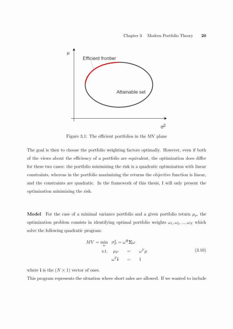
Chapter 3 Modern Portfolio Theory 20
Figure 3.1: The e�cient portfolios in the MV plane
The goal is then to choose the portfolio weighting factors optimally. However, even if both
of the views about the e�ciency of a portfolio are equivalent, the optimization does di↵er
for these two cases: the portfolio minimizing the risk is a quadratic optimization with linear
constraints, whereas in the portfolio maximizing the returns the objective function is linear,
and the constraints are quadratic. In the framework of this thesis, I will only present the
optimization minimizing the risk.
Model For the case of a minimal variance portfolio and a given portfolio return µp, the
optimization problem consists in identifying optimal portfolio weights !1,!2, ...,!N which
solve the following quadratic program:
MV = minw
�2P = !
T⌃!
s.t. µP = !Tµ
!Ti = 1
(3.10)
where i is the (N ⇥ 1) vector of ones.
This program represents the situation where short sales are allowed. If we wanted to include

Chapter 3 Modern Portfolio Theory 21
the condition that only long positions are allowed in the model, we should add the constraint
!i � 0.
The solution of the constrained quadratic optimization problem presented above has been
derived by Merton (1972). The latter has proved this problem can be solved using the method
of Lagrange multipliers. A more detailed exposition of the results can be found on the paper
written by Merton.
!⇤ = µpg+ f (3.11)
with
g =1
d(c⌃�1µ� b⌃�1
i) (3.12)
f =1
d(b⌃�1µ� a⌃�1
i) (3.13)
with a = µ0⌃�1µ, b = µ0⌃�1i, c = i
0⌃�1i and d = ac� b
2. The portfolio standard deviation
is given by
� =
r1
d(cµ2
P � 2bµp + a) (3.14)
The portfolio which minimizes the variance for a specified expected return is called a ”frontier
portfolio”. It follows from this equation that all frontier portfolios !⇤ are a linear combina-
tion of two portfolios f and g. The equation of the portfolio standard deviation represents
the ”e�cient frontier”, a hyperbola for mean-variance portfolios as represented in figure 3.1.
Concretely, this e�cient frontier consists of the set of all e�cient portfolios that yield the
highest return for each level of risk, as mentioned above, and provides an elegant way to
achieve an e�cient allocation: a higher expected return can only be achieved by taking on
more risk. An interesting e�cient allocation to focus on is the one at the bottom of the
e�cient frontier. This point constitutes the portfolio with the smallest variance among all
feasible portfolios, or in other words, the portfolio with the minimum risk but also the mini-
mum return. It is called the global minimum variance (GMV) portfolio.
Chapter 3 Modern Portfolio Theory 22
Over the last several years, minimum variance portfolio has attracted more and more of
investor’ attention. This gain in popularity can be explained by two things. Firstly, the
latest financial crisis has emphasized the importance of risk management and a minimum-
variance strategy is obviously one of the perfect way to address it. And secondly, recent
papers8 support the long-standing critique of the CAPM (see section 3.2) that high-risk
stocks don’t always lead to high-return, as demonstrated by Fama and French (1992), mean-
ing that a portfolio construction based on the minimum-variance principle could represent a
highly e�cient solution for portfolio selection.
The minimum variance portfolio is a specific portfolio on the mean-variance e�cient frontier,
very easy to compute and presenting a unique solution which is recognized to be robust since
the portfolio ignore estimates of the expected returns9. The optimization function can simply
be written as:
GMV = minw
!T⌃!
s.t. !Ti = 1
(3.15)
Its weights are given by !⇤GMV = ⌃�1
i/i0⌃�1
i. We can observe that the weights can be
thought of as a limiting case of the equation 3.10, if a mean-variance investor ignores the
constraint on expected returns.
Assumptions The mean-variance analysis described above comes necessary with some
assumptions. Their validity have been largely disused by the practitioners so I will only
enumerate them here but the empirical results of Markowitz’s MV model is presented in
section 4.3:
• All investors are risk averse, meaning they prefer less risk to more for the same level of
expected return8As an example, Ang et al. (2006) published a paper where they document a low-risk and high-return
empirical anomaly that they associate with idiosyncratic risk.9The empirical problems of the MV model are discussed in section 3.3. However, it is important to
mention that in this case, the expected returns do appear in the estimated covariance matrix, but it has
been proved by Morrison (1990) that, under the assumption of Normal asset return, for any estimator of the
covariance matrix, the MLE estimator of the mean is always the sample mean. This allows one to remove
the dependence on expected returns for constructing the MLE estimator of the covariance matrix.

Chapter 3 Modern Portfolio Theory 23
• Expected returns for all assets are known
• The variances and covariances of all asset returns are also known
• Investors need to know only the expected returns, variances, and covariances of re-
turns to determine optimal portfolios. They can ignore skewness, kurtosis, and other
attributes of a distribution
• There are no transaction costs or taxes
3.2 Capital Market Line and the CAPM Model
Following Markowitz’s model, an investor is only interested in the mean and variance of the
return on his portfolio and will therefore invest in one that is e�cient in the mean-variance
way. Based on this framework, Sharpe (1964) and Lintner (1965) developed an equilibrium
model, called the Capital Asset Pricing Model or CAPM, by adding two key assumptions to
the Markowitz model. The first one is that investors have identical views about risky assets
mean returns, variances of returns, and correlations and the second one is that investors can
borrow and lend at the risk-free rate without limit, and they can sell short any asset in any
quantity.
The introduction of the second assumption, so allowing a portfolio to include risk-free se-
curity has an interesting e↵ect: it turns the e�cient frontier into a straight line, called the
Capital Market Line, that is tangential to the risky e�cient frontier and with a y-intercept
equal to the risk-free rate. We can see from figure 3.2 that all e�cient portfolios are a com-
bination of the risk-free rate and a single risky tangency portfolio, T. This result comes from
Tobin’s (1958) ”separation theorem” and the tangency portfolio T is the optimal portfolio
only composed of risky assets.
As a summary, every investor that is a mean-variance optimizer will hold the same tangency
portfolio of risky assets in conjunction with a position in the risk-free asset. So, because all

Chapter 3 Modern Portfolio Theory 24
investors hold the tangency portfolio and because the market must clear, the T portfolio is
referred as the market portfolio.
Figure 3.2: E�cient frontier with a risk-free asset
Note: the figure comes from Fama and French (2003)
The equation of the capital market line (CML), and thus of the CAPM can be derived as
E[Ri] = rf + [E[RM ]� rf ]�iM (3.16)
where E[Ri] is the expected return on asset i and �iM is the market beta of asset i, defined
by the ratio of the covariance of its return with the market return and the variance of the
market return, �iM = cov(Ri,RM )�2(RM ) . The interpretation of beta is that it measures the volatility
of a security or portfolio in comparison to that of the market as a whole. In our case of
portfolio selection, the beta represents the volatility of an asset composing the portfolio in
comparison to the total volatility of the portfolio and is defined by �iP = cov(Ri,RP )�2P
. In fact,
beta is a measure of the systematic risk.
This equation can be interpreted as follows: the expected return on a security or a port-
folio is equal to the risk-free rate (rf ) plus a risk premium. And the risk premium on a stock
Chapter 3 Modern Portfolio Theory 25
or portfolio varies directly with the level of systematic risk (beta). So concretely the security
market line shows the risk or expected return tradeo↵ that exists with the CAPM. As stated
earlier, since the idiosyncratic (unsystematic) risk can be eliminated through diversification
by holding a large portfolio, more return means that an investor must take more systematic
risk.
Another interesting element to look at is the slope of the CML, which is E[RM ]�rf�RM
, also
known as the Sharpe ratio. This ratio represents the expected excess return of a portfolio to
the portfolio’s volatility, or in other words the expected excess return per unit of risk. The
Sharpe optimal portfolio is the one with maximum Sharpe ratio, which is nothing more than
the tangency portfolio.
3.3 Empirical results of Markowitz’s Mean-Variance
Model
Despite its simplicity of comprehension and utilization, the traditional mean-variance model
of Markowitz has many shortcomings when applied in practice. Theses shortcomings are
mainly related to estimation errors. Indeed, we do not know in practice the true value of the
parameters µi and �i. We therefore have to replace these unknown parameters by estimates,
based on historical data and this obviously leads to estimation errors, which have a direct
impact on the portfolio weights so that the desired properties of diversification are no longer
met. The problems resulting from estimation errors are as follows:
1. Extreme allocations and sensitivity: the first problem we encounter with the MV anal-
ysis is that it tends to produce portfolios composed of combinations of extreme shorts
and extreme longs, which are very sensitive to a change in the inputs. For example,
Chopra (1993) has shown that small changes in the input mean-variance parameters
lead to large variations in the composition of the optimal portfolio.
Chapter 3 Modern Portfolio Theory 26
2. Estimations of the returns: weights of the optimal portfolio tend to be extremely
sensitive to very small changes in the expected returns. For example, a small increase
of the expected return of one asset can greatly alter the optimal portfolio’ composition.
Best and Grauer (1991) have demonstrated that and have also showed that the more
assets there are in a feasible set, the more sensitive MV-e�cient portfolio will be to
changes in the means. Also, one of the result of Kallberg and Ziemba (1984) is that
estimation errors in the means are about ten times as important as estimation errors
in variances and covariances.
3. Estimation in variances and covariances: errors in estimated covariance matrices can
also have considerable impact. Chopra and Ziemba (1993) demonstrated that, at a
lower risk tolerance, the relative impact of errors in mean, variance and covariances is
closer. However, the problems linked to variance and covariance’ estimation errors can
be mitigated to varying extents through the use of more robust estimation techniques,
as we will see it later.
4. Amplification of large estimation errors: it has also been shown (Jobson and Korkie
(1981), Michaud (1989)) that optimal portfolio tends to amplify large estimation errors
in certain directions. Indeed, the risk of the estimated optimal portfolio is typically
under-predicted and its return is over-predicted: if the variance of an asset appears to
be small, or similarly the mean return of this asset appears to be large, as a result of
being significantly underestimated, or overestimated respectively, the optimal portfolio
will assign a large weight to it.
The major result of these estimation errors is that optimal MV portfolios are often extremely
concentrated on a few asset, and this is clearly not in line with the notion of diversification.
Beside from the estimation errors, the Mean-Variance approach allows extreme concentrations
to occur by creating optimal portfolios composed of few assets which are presenting the
highest (expected) returns (Bernstein, 2001). Many authors, such as Green and Hollifield
(1992), Bera and Park (2008) or Yu, Lee and Chiou (2014) have published on the subject and
proposed solutions to deal with this issue. The content of the following sections will thus be

Chapter 3 Modern Portfolio Theory 27
focused on the presentation of several diversification measures. Once the presentation will be
made, we will analyze their results and see if they meet some criteria that any diversification
measures must have to be named as such. These criteria and the reason of their selection
will be developed in the chapter 5, as well as the description of the dataset and methodology
we used to perform our analysis.
Chapter 4
From MV Selection to Alternative
Methods
As we have seen, the use of Markowitz approach to create an optimal portfolio has proved
to be problematic. Indeed, the method requires the expected return and variance of each
security, and we have seen that the estimation of theses parameters leads to errors which re-
sult in the creation of optimal portfolios excessively concentrated in a limit number of assets.
Therefore, the use of the MV method to construct a well-diversified portfolio doesn’t seems
to be the best choice. Moreover, the results shown by this method are clearly in contradiction
with the notion of diversification that we have presented in chapter 2.
In the following chapter, we will present some measures of diversification that have been
developed over the past few years. These measures can be grouped into the three following
categories:
1. Entropy Measures
2. Risk-based allocation
3. Diversification with regard to Risk Factors
28
Chapter 4 From MV Selection to Alternative Methods 29
4.1 Entropy Measures
Entropy is a concept which was originally introduced in the information theory by Shannon
(1948) and was defined in a statistical mechanics framework. Although it was not initially
made to be applied in the portfolio management field, some interesting studies have been
written on the subject and its use as an alternative measure of risk is now an established fact.
The first authors who have used entropy in a portfolio optimization framework were Philip-
patos and Wilson (1972). Since then, many other related works such as Hua and Xingsi
(2003), Bera and Park (2008) or Meucci (2009) have been published. In the framework of
this thesis aiming to review and analyze measures allowing to assess the diversification of
investment portfolios, we will focus our attention on the Shannon entropy and the diversifi-
cation delta.
4.1.1 Shannon Entropy and Equally Weighted Portfolio
As mentioned, many academic and practitioner’s literature have proposed to use entropy
approach to optimal portfolio selection. The main idea of this approach is to use entropy
measure as the objective function for the optimization problem. In this case, weights of the
portfolio are considered as the probability mass function of a random variable. We can obtain
a pretty well-diversified portfolio by maximizing the entropy measure for such a random vari-
able which are subject to some given constraints. Moreover, using entropy as the objective
function guarantees non-negative weights for the assets in the portfolio, as they are seen as
probabilities, which by definition take non-negative values.
Statistically, the concept of entropy can be resume as follows: it is a probabilistic mea-
sure of uncertainty or disorder. Basically, the entropy of a random variable is the ”amount of
information” contained in this variable: the more information it contains, the more order it
has. Entropy is therefore a useful tool which is able to quantifies the amount of information
in a random variable, which provides a good measure of the disorder present in a probability
Chapter 4 From MV Selection to Alternative Methods 30
distribution. The most prominent entropy measure is surely the Shannon’s entropy (H). In
a portfolio construction framework, it allows to shrink the weight of the assets toward an
equally weighted portfolio. It has the following form:
H(!) = �NX
i=1
!i log!i, (4.1)
where ! = (!1,!2, ...,!N ) is a portfolio allocation among N risky assets with properties thatPN
i=1 !i = 1, !i � 0 and i = 1,2...,N.
The maximum value of H(!) is reached when !i = 1/N, for all i = 1, ..., N and the other
extreme case occurs when !i = 1 for one i, and = 0 for the rest, then H(!) = 0.
The Shannon’s Entropy form that we used in our analysis is the exponential form:
H(!) = exp⇣�
NX
i=1
!i log!i
⌘, (4.2)
The measure reach a minimum equal to 1 if a portfolio is fully concentrated in a single
component and a maximum equal to N , representing an Equally Weighted Portfolio.
A word on the Equally Weighted Portfolio The equally weighted portfolio that leads
to a maximum value of H is a naive but well-known strategy in portfolio management. In-
deed, investors are still using such simple allocation rules for allocating their wealth across
assets even though other more sophisticated theoretical models have been developed in the
last 60 years.
Besides the fact that it is computationally simple to implement, it has been proved that
the 1/N asset allocation strategy can have a ”higher out-of-sample Sharpe ratio, a higher
certainty-equivalent return, and a lower turnover than optimal asset allocation policies”
(DeMiguel et al. (2005)). Comparable results have been shown in Bloomfield et al. (1997),
Jorion (1985) and Bera and Park (2008). Moreover, it does not involve any estimation or
optimization and it also completely ignores the data. All it requires is to hold a portfolio
with equal weights, so that !i = 1/N in each of the N risky assets.
A quick comparison can be made between this strategy and the one describes by the equation
3.10. Indeed, the 1/N portfolio can be seen as a strategy that does estimate the expected
Chapter 4 From MV Selection to Alternative Methods 31
returns and covariance matrix, but imposes the restriction that expected returns are pro-
portional to total risk rather than systematic risk, which can be mathematically written like
µi / ⌃i1N .
4.1.2 Diversification Delta
The diversification delta is an entropy-based ratio that has been originally developed by
Vermorken et al. (2012). It can be defined as the ratio of the weighted average entropy
of the assets minus the entropy of the portfolio divided by the weighted average entropy of
the assets. Here, the exponential entropy is used. This idea, suggested by Campbell (1966)
but also mentioned as a risk measure in Fabiozzi (2012), allows ”to avoid singularities of the
entropy while still letting the uncertainty speak for itself”.
Formally, for a given portfolio consisting of N risky assets (X1, ..., XN) and weights (!1, ...,!N),
withPN
i=1 !i = 1, the diversification delta developed by Vermorken et al. (2012) can be de-
fined as the following ratio:
DD(P ) =exp(
PNi=1 !iH(Xi))� exp(H((
PNi=1 !iXi))
exp((PN
i=1 !iH(Xi))(4.3)
where f is the probability density function of X and H(X) = �Rx[f(x)]log(f(x))dx is the
di↵erential entropy that is used as a measure of uncertainty.
The interpretation of this ratio is as follows: it is a ratio that compares the weighted individual
assets and the portfolio. The diversification delta is ”designed to measure the diversification
e↵ect of a portfolio by considering the entropy of the assets and comparing it with the entropy
of the portfolio”. Therefore, the higher the level of entropy, the higher the uncertainty and
inversely. The possible values of the ratio are ranged between 0 and 1.
The use of such ratio that compares the uncertainty of individual assets with the uncer-
tainty of the portfolio is an interesting way to analyze a portfolio and quantify the e↵ect
of diversification. However, the diversification delta presents several issues as demonstrated
by Salazar et al. (2014). By using the required properties of a risk measure as described

Chapter 4 From MV Selection to Alternative Methods 32
in section 2.1.2, they have demonstrated that sub-additivity is not satisfied in the definition
of the diversification delta. This entails the ratio can be negative but it also means it is
not left bounded. Moreover, Salazar et al. (2014) have also shown that the left-hand side
in the numerator of equation 4.2 is not homogeneous, meaning that ”changes in the size of
the assets are not detected in the same way as changes in the portfolio” and this leads to
inconsistencies in the measurement of diversification.
Therefore, in order to address these issues, Salazar et al. (2014) have proposed to use the
exponential entropy as a measure of uncertainty and formulated the following revised diver-
sification delta DD*:
DD⇤(P ) =
PNi=1 !iexp(H(Xi))� exp(H((
PNi=1 !iXi))PN
i=1 !iexp(H(Xi))(4.4)

Chapter 4 From MV Selection to Alternative Methods 33
4.2 Risk-based Allocation: Diversification ratio and
Marginal Risk Contributions
In this section, we will present two diversification measures based on a portfolio’s risk assess-
ment and management which have been quite popular over the last years. These measures
are respectively named the Diversification ratio and the Marginal Risk Contributions.
4.2.1 Diversification Ratio
The Diversification ratio (DR) has been introduced in 2008 by Choueifaty and Coignard.
This diversification measure can be defined as the ratio of a portfolio’ weighted average of
volatilities divided by its overall volatility. In essence, the DR measures ”the diversification
gained from holding assets that are not perfectly correlated” (Choueifaty et al. (2013)).
Another way to represent the DR is to consider a portfolio which is exposed to F independent
risk factors. Also, the portfolio’s exposure to each risk factor is inversely proportional to the
factor’s volatility so that the risk budget of this portfolio is equally allocated across all
risk factors and the DR2 = F , meaning that the DR squared is equal to the number of
independent risk factors represented in a portfolio.
Formally, given a portfolio composed of N assets (X1, ..., XN) and weights (!1, ...,!N), withPN
i=1 !i = 1, we have:
DR =
PNi=1 !i�i
�P(4.5)
where �i is the volatility of asset i and �P the portfolio volatility. According to Choueifaty et
al. (2013), the DR ”embodies the very nature of diversification”: the volatility of the overall
(long-only) portfolio is less than or equal to the weighted sum of the assets volatilities.
In order to completely understand the intuition behind this ratio, an interesting decom-
position of it has been formalized in Choueifaty et al. (2013). The decomposition has the
following form:
DR(w) = [⇢(w)(1� CR(w)) + CR(w)]�1/2, (4.6)

Chapter 4 From MV Selection to Alternative Methods 34
where ⇢(w) is the volatility-weighted average correlation of the assets in the portfolio and
CR(w) is the volatility-weighted concentration ratio (CR) of the portfolio. These two are
defined by
⇢(w) =
PNi 6=j(!i�i!j�j)⇢ijPN
i 6=j(!i�i!j�j)(4.7)
CR(w) =
PNi=1(!i�i)2
(PN
i=1 !i�i)2(4.8)
From these equations, it can be seen that a portfolio which has a high concentration in few
assets, or a portfolio consisting of highly correlated assets will have a low DR and therefore
can be described as poorly diversified. In other words, the DR increases when ⇢(w) and, or
CR(w) decreases and inversely.
The extreme case of a DR equal to 1, representing a fully concentrated, mono-asset portfolio,
is reached when correlations between assets or the CR is equal to 1.
4.2.2 Risk Parity and Marginal Risk Contributions
Risk Parity
The term ”marginal risk contributions” comes from a portfolio construction strategy named
the risk parity. The general idea behind the risk parity approach is that each asset, or asset
class (such as bonds, stocks, commodities, interest rates, etc.), doesn’t have the same contri-
bution to the total risk of a portfolio. Therefore, to build a diversified portfolio, we need to
focus on the amount of risk that each component i composing the portfolio represents rather
than on the specific weight invested in each component i. In other words, instead of being
focused on the allocation of capital like the ”traditional” methods, risk parity is focused on
the allocation of risk.
One could see risk parity as a mix between the minimum variance and the equally-weighted
portfolios as described above. Indeed, the risk parity approach can be located between the
Chapter 4 From MV Selection to Alternative Methods 35
minimum variance and equally-weighted portfolios because roughly speaking, building a risk
parity portfolio is similar to create a minimum-variance portfolio subject to the constraint
that each asset, or asset class, contributes equally to the total portfolio risk8.
The approach has gained a lot of popularity in the last years and basically became stan-
dard practice for institutional investors. Some of them even claims it is the most e�cient
one. For example, Qian (2011) said that risk parity allocation results in better diversification
and brings higher returns. One of the main advantage of the risk parity approach is that
we do not need to use some estimation of expected returns. Indeed, as we have seen in the
section 3.3, forecasting returns is a risky business and leads to estimation errors. On the
other hand, the risk parity approach requires some accurate estimations of the variances and
covariances, but robust estimation techniques exist (se for example Ledoit and Wolf (2004))
and have been proven to be relatively stable. Therefore, it is possible to estimate variances
and covariances with a good deal of accuracy.
Marginal Risk Contributions
To measure the share of the total portfolio risk which is attributable to a component i, or
simply the risk contribution of a component i, we have to compute the product of the allo-
cation in i with its marginal risk contributions, which is given by the change in the total risk
of the portfolio induced by an infinitesimal increase in holdings of component i. Therefore,
in this context, a well-diversified portfolio is the one where all asset classes have the same
marginal contribution to the total risk of the portfolio.
Based on the use of standard deviation as the measure of the total risk of a portfolio, we
can calculate the contribution of each asset class to it. The marginal risk contributions of an
asset class, noted @xi�P , is given by the following expression:
@!i�P =@�P
@!i=!i�
2i +
Pj 6=i !j�ij
�P(4.9)
8Proof of that can be found in Maillard, S., Roncalli, T., and Teiletche, J. (2009)
Chapter 4 From MV Selection to Alternative Methods 36
As mentioned, the total risk contribution from an asset i is computed as the product of
the allocation in asset i with its marginal risk contribution. The risk contribution of i can
therefore be written as:
RCi = �i(!) = !i ⇥ @!i�P = !i
!i�2i +
Pj 6=i !j�ij
�P(4.10)
And the total risk of the portfolio is thus nothing more than the sum of the total risk
contributions,
TR =NX
i=1
RCi =NX
i=1
�i(!) (4.11)
The measure that we will use in our analysis is the risk contribution RCi.
Chapter 4 From MV Selection to Alternative Methods 37
4.3 Diversification with regards to Risk Factors
The following measures of diversification are based on one of the best-known techniques in
multivariate analysis, the Principal Components Analysis or PCA. The attractive character-
istic of PCA is that it has the ability to decompose correlated variables into uncorrelated
components, which can obviously be very interesting to use when we are trying to analyze
the complex structure of financial markets. Indeed, PCA provides us with a way to identify
uncorrelated risk sources in the market and pick stocks from those di↵erent risk sources.
Therefore, after applying PCA for a stock picking purpose, the resulting portfolio size is
more meaningful from the point of view of diversification.
Partovi and Caputo (2004) were the first to propose the idea of using PCA in the portfolio
selection framework. Their basic idea was based on the fact that if there were no correlations
among assets, the complexity in portfolio selection dramatically decreased. Since the pub-
lication of their paper, Partovi and Caputo (2004) have inspired many academic researcher
but also many portfolio managers to construct principal portfolios (uncorrelated portfolios),
especially when risk reduction and management became the priority, after the financial crisis
of 2008.
Here we will present two interesting diversification indexes which are based on the theoreti-
cal framework of PCA: the Portfolio Diversification Index, developed by Rudin and Morgan
(2006), and the E↵ective Number of Bets, developed by Meucci (2009).
4.3.1 Brief Review of the Principal Component Analysis
Principal Component Analysis (PCA) is a statistical method of dimension reduction that is
used to reduce the complexity of a data set while minimizing information loss. It transforms
a data set in which there are a large number of correlated variables into a new set of uncorre-
lated variables, called the principal components. The first principal component account for
as much of the variability as possible, and each succeeding component accounts for as much
of the remaining variability as possible. Each principal component is a linear combination of

Chapter 4 From MV Selection to Alternative Methods 38
the original variables in which the coe�cients indicate the relative importance of the variable
in the component.
Consider the linear combinations
Y1 = e11X1 + e12X2 + e1pXp
Y2 = e11X1 + e22X2 + e2pXp
...
Y1 = ep1X1 + ep2X2 + eppXp
This can be seen as a linear regression where we are predicting Yi from X1, X2, ..., Xp. There
is no intercept but ei1, ei2, ..., eip can be viewed as regression coe�cients.
Formally, the variance and covariance are written as
var(Yi) = e0
i⌃ei = �i (4.12)
cov(Yi, Yj) = e0
i⌃ej (4.13)
where �1,�2, ...,�p are the eigenvalues of the variance-covariance matrix ⌃ and the vectors
e1, e2, ..., ep are the corresponding eigenvectors.
The goal of the PCA is, for the ith principal component Yi, to select ei1, ei2, ..., eip such that
var(Yi) is maximized with the constraints that the sum of squared coe�cients add up to one
and each new component defined is uncorrelated with all the previously defined components.
Formally, we have to maximize var(Yi) = e0i⌃ei subject to the constraints:
e0
i⌃ei = 1 (4.14)
cov(Y1, Yi) = e01⌃ei = 0,
cov(Y2, Yi) = e02⌃ei = 0,
...
cov(Yi�1, Yi) = e0i�1⌃ei = 0

Chapter 4 From MV Selection to Alternative Methods 39
4.3.2 Portfolio Diversification Index
The Portfolio Diversification Index is a measure developed by Rudin and Morgan (2006)
which quantify the diversification distinctly related to correlations. Concretely, the PDI in-
dicates the diversification’ level of a given portfolio and can assess whether the addition of
new assets to the portfolio improves its diversification and by how much (Smith (2006)).
Therefore, this index can be compared to the Diversification Ratio, as described above. In-
deed, these two measures both aim to quantify the diversification distinctly related to corre-
lations and provide frameworks for constructing diversified portfolio (Randy O’Toole (2014)).
Given a portfolio consisting of N risky assets, the equation for the PDI is as follows:
PDI = 2NX
i=1
iRSi � 1, (4.15)
where RSi =�iPNj=1 �j
is the relative strength of the ith principal component, �i being the
eigenvalue associated with the ith principal component. From this equation, we can see that
the diversification properties of a portfolio are ”conveyed by means of the relative strength of
these factors” (Smith, 2006).
The PDI can have values comprised between 1 and N and the interpretation of these extreme
cases is as follows:
• A PDI = 1 represents a portfolio dominated by a single factor and thus completely
undiversified. In that case, RS1 ⇡ 1 and the others are null.
• a PDI = N represents a portfolio totally diversified. In that case, RSi ⇡ 1/N for all i.
It is thus straightforward that a high PDI value indicates a well-diversified portfolio and
inversely, a low PDI value indicates a less diversified portfolio.

Chapter 4 From MV Selection to Alternative Methods 40
4.3.3 E↵ective Number of Bets
Another use of PCA in a portfolio construction framework can be found in Meucci (2009). In
his paper, Meucci proposed to transform a data set composed of a large number of correlated
assets into a new set of principal portfolios representing uncorrelated risk sources related to
the original assets. He then introduced a ”diversification distribution”, a tool to analyze the
structure of a portfolios concentration profile. The diversification distribution is expressed as
the ratio of each principal portfolios variance to its total variance. In this principal portfolio
environment, all the principal portfolios are uncorrelated and therefore the total variance of
the portfolio can be written as a sum of the contributions of each factor’s variance. The
ratio of individual principal portfolio variance to the total variance is then in the range of
0 to 1 and sum to 1. Here the maximum diversification is reached when the diversification
distribution is close to one. Therefore, based on this method, a well-diversified portfolio is
the one in which all the risk sources composing it are invested equally.
Moreover, Meucci (2009) introduced a diversification index that represented the e↵ective
number of uncorrelated bets (ENB) in a portfolio. The idea is that if the number of uncorre-
lated bets were small, the risks were rather concentrated in few sources and less diversified.
The construction of a portfolio following such method could be compared to the one fol-
lowing the risk parity approach, as described above. These two allocations strategy present
a similarity even if they are conceptually di↵erent. Indeed, they both construct portfolios by
allocating risks. But the way these two strategies allocate risk is completely distinct. The risk
parity strategy allocates investments in such a way that they equally contribute to the risk of
the total portfolio whereas the ENB strategy allocates risk based on uncorrelated principal
portfolios. The consequence is that risk parity allocation strategy can have rather concen-
trated risk if most assets have high correlations with each other. As an example, consider
an extreme case with all stocks perfectly positive correlated. The result is that allocating
equal risk budget to all stocks is actually the same as holding one stock. The ENB strategy
does not have such a problem since it is allocating its risk budget based on uncorrelated risk

Chapter 4 From MV Selection to Alternative Methods 41
sources. Though in the case of perfect correlations all variation would be explained by the
first principal component.
Formally, the development of Meucci (2009) began with the decomposition of the the variance-
covariance matrix ⌃ of the N assets:
E0⌃E = ⇤ (4.16)
where ⇤ ⌘ diag(�1,�2, ...,�N) is a diagonal matrix. The columns of ⇤ are the respec-
tive eigenvectors E ⌘ (e1, e2, ..., eN) which define a set of N uncorrelated portfolios (prin-
cipal portfolios). The returns of the principal portfolios can be expressed as rF = E0R,
where R denotes the random returns on the N assets, and the variances are the eigenvalues
(�1,�2, ...,�N). Following that, the original portfolio ! can be expressed as a combination of
the uncorrelated principal portfolios with weights !F = E�1!.
Also, the introduction of uncorrelated factors allows to write the total variance of the portfolio
as the sum of the contributions of each factor’s variance:
!0⌃! =
NX
i=1
!2Fi�
2i (4.17)
The contribution of the ith factor to the total portfolio variance is defined by what Meucci
calls the diversification distribution: pi(!) =!2Fi�
2iPN
i=1 !2Fi�
2i
. Each pi(!) is positive and their
sum equal to 1.
The interpretation given by Meucci (2009) to the diversification distribution is that it rep-
resents a set of probability masses associated with the principal portfolios and therefore, a
portfolio ! is well diversified when ”the probability masses pi are approximately equal and thus
the diversification distribution is close to uniform”. Moreover, by measuring the dispersion
of the probability distribution, which can be done thanks to its entropy, we can thus measure
the diversification of the portfolio.
ENB(!) = exp⇣�
NX
i=1
pi(!)ln(pi(!))⌘
(4.18)

Chapter 4 From MV Selection to Alternative Methods 42
A maximal value of ENB(!) equal to N would mean that the risk is evenly spread amongst
the di↵erent factors and the portfolio is thus well diversified portfolio, whereas a value of
ENB(!) equal to 1 would mean that the portfolio is concentrated in a single risk factor.

Chapter 5
Data and Methodology
In this chapter, we describe the methodology that has been followed in order to conduct our
studies on the diversification measures presented in chapter 4. The goal of the analysis is
obviously to provide answers to the research questions raised in the chapter 1.
To realize that, we will first describe the data that have been collected. Then we will present
the procedure we followed in order to perform our analysis. The implementation of Shannon’s
Entropy will be also described in this section. Finally, we will analyze the results obtained
and try to answer the research questions that we put these measures in relation with the
criteria selected to see if they meet the requirements that define a diversification measure.
The computer program chooses to complete our analysis is Matlab. The scripts that we used
can be found on the DIAL website, under the file linked to the electronic version of this
thesis.
5.1 Description of the Data
Database
The data used in our empirical study were obtained on Bloomberg and are based on a weekly
basis for the period from 29 December 1989 to 4 May 2018, which provides 1,480 weekly
returns. The prices showed correspond to the closing prices of each Friday. Also, we consider
43
Chapter 5 Data and Methodology 44
the following five asset classes:
• US large capitalization stocks: we used the S&P 500 equity index as a proxy. This index
represent a market value weighted index of the 500 larger cap companies in the United
States. It is constructed by adjusting the closing S&P 500 closing prices to corporate
actions (S&P Global (2016)). The index is denoted by the ticker SPXT Index.
• US Treasury bonds: we used the S&P US Treasury Bond Index as a proxy. This index
is a market-value weighted index that seeks to measure the performance of the United
States Treasury Bond Market. Treasury Bond, or Treasury-bill (T-bill), is a short-term
debt obligation backed by the U.S. government with a maturity of less than one year
(definition from Investopedia). It is seen as the safest investment that can be made,
which explain why a T-bill investment is usually referred as risk-free. It is denoted by
the ticker SPBDUSBT Index.
• Commodities: we used the S&P Goldman Sachs Commodity Index as a proxy. This
index is the first major commodity index which was originally developed by Gold-
man Sachs. It is designed to be investable by including the most liquid commodity
futures9. The index currently comprises 24 commodities from all commodity sectors:
energy products, industrial metals, agricultural products, livestock products and pre-
cious metals. It is denoted by the ticker SPGSCITR Index.
• US corporate bonds: we used the SPDR Bloomberg Barclays U.S. Corporate Bond
Index (Bloomberg Barclays U.S. Corporate Total Return Value Unhedged USD) as a
proxy. This index ”measures the performance of the investment grade U.S. corporate
bond market” (State Street Global Advisors (2018)). Each security that are included
into the index must be fixed rate, in U.S. dollar, taxable and rated investment grade
as defined by the Index methodology. It is denoted by the ticker LUACTRUU Index.
• Real Estate: we used the Dow Jones Equity All REIT Index as a proxy. This index is
designed to ”measure all publicly traded real estate investment trusts in the Dow Jones
9A commodity is a basic good used in commerce such as oil, sugar, rice, etc.
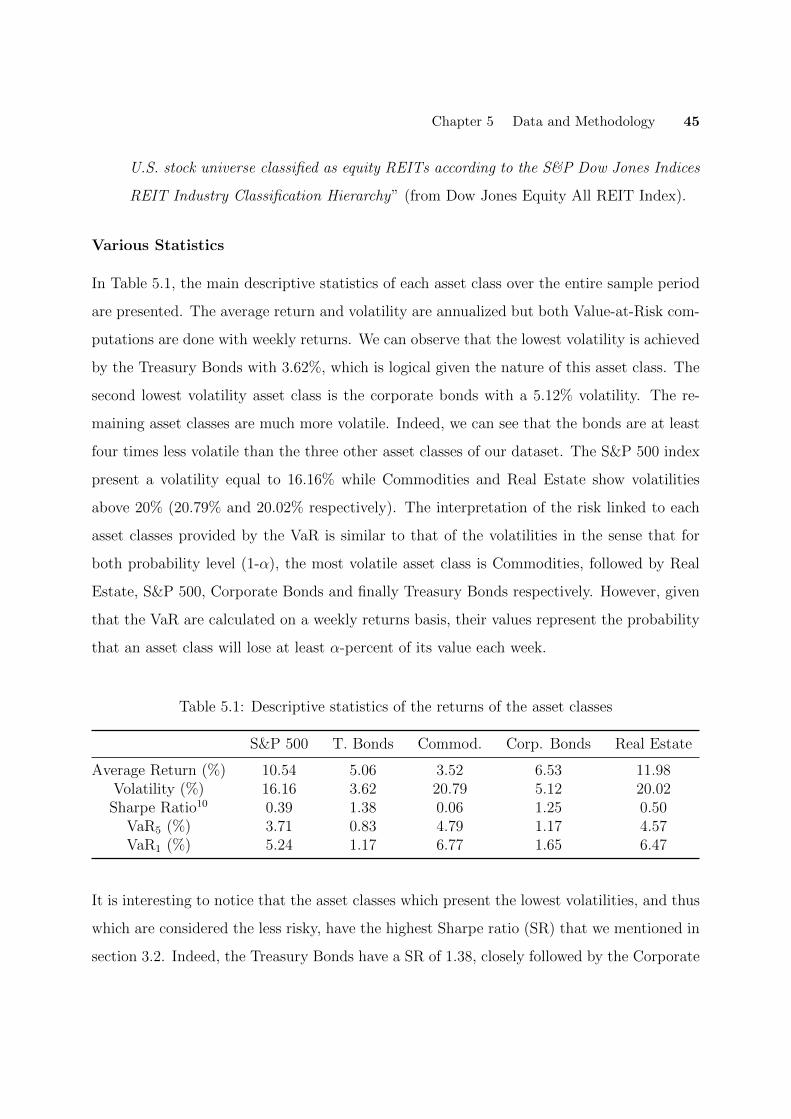
Chapter 5 Data and Methodology 45
U.S. stock universe classified as equity REITs according to the S&P Dow Jones Indices
REIT Industry Classification Hierarchy” (from Dow Jones Equity All REIT Index).
Various Statistics
In Table 5.1, the main descriptive statistics of each asset class over the entire sample period
are presented. The average return and volatility are annualized but both Value-at-Risk com-
putations are done with weekly returns. We can observe that the lowest volatility is achieved
by the Treasury Bonds with 3.62%, which is logical given the nature of this asset class. The
second lowest volatility asset class is the corporate bonds with a 5.12% volatility. The re-
maining asset classes are much more volatile. Indeed, we can see that the bonds are at least
four times less volatile than the three other asset classes of our dataset. The S&P 500 index
present a volatility equal to 16.16% while Commodities and Real Estate show volatilities
above 20% (20.79% and 20.02% respectively). The interpretation of the risk linked to each
asset classes provided by the VaR is similar to that of the volatilities in the sense that for
both probability level (1-↵), the most volatile asset class is Commodities, followed by Real
Estate, S&P 500, Corporate Bonds and finally Treasury Bonds respectively. However, given
that the VaR are calculated on a weekly returns basis, their values represent the probability
that an asset class will lose at least ↵-percent of its value each week.
Table 5.1: Descriptive statistics of the returns of the asset classes
S&P 500 T. Bonds Commod. Corp. Bonds Real Estate
Average Return (%) 10.54 5.06 3.52 6.53 11.98Volatility (%) 16.16 3.62 20.79 5.12 20.02Sharpe Ratio10 0.39 1.38 0.06 1.25 0.50
VaR5 (%) 3.71 0.83 4.79 1.17 4.57VaR1 (%) 5.24 1.17 6.77 1.65 6.47
It is interesting to notice that the asset classes which present the lowest volatilities, and thus
which are considered the less risky, have the highest Sharpe ratio (SR) that we mentioned in
section 3.2. Indeed, the Treasury Bonds have a SR of 1.38, closely followed by the Corporate

Chapter 5 Data and Methodology 46
Bonds with a SR of 1.25. In comparison the latter asset classes, the S&P 500 and Real Estate
index have much higher average returns, but their respective high volatilities lead to a much
lower SR (0.39 and 0.50 respectively).
Table 5.2 presents the correlations between de di↵erent asset classes. We can see that the
Treasury and Corporate bonds are negatively correlated with all the other asset classes ex-
cept with each other, presenting a highly positive correlation (93.07%). Commodities are
also negatively correlated with all the other classes and doesn’t seem to present any correla-
tion with the equity stocks (S&P 500). Finally, Real Estate appear to be highly positively
correlated with the S&P 500 Index.
Table 5.2: Correlation Matrix in %
S&P 500 T. Bonds Commod. Corp. Bonds Real Estate
S&P 500 100 -80.11 3.08 -58.24 80.46Treasury Bond -80.11 100 -60.31 93.07 -66.97Commodities 3.08 -60.31 100 -75.62 -4.67
Corporate Bonds -58.24 93.07 -75.62 100 -42.53Real Estate 80.46 -66.97 -4.67 -42.53 100
To apply the ENB and PDI measures, we have also performed a Principal Component Analy-
sis (PCA) on the variance-covariance matrix estimated over the entire database. This allows
us to identify the factors that a↵ect the returns of each asset classes. The results are given in
the Table 5.3 below. Concretely it shows the e↵ects, or exposures, of each of the factors on
the di↵erent asset classes11. The variance of each factor represents the eigenvalues that are
obtained after performing the PCA, as explained in section 4.3.1. Moreover, all the factors
are obviously uncorrelated and explain the entire variability of the asset classes’ returns. The
interpretation of the factors resulting from the PCA is as follows:
• With an exposure equal to 82.99%, the first factor F1 seems to be related to the real
estate risk. Also, we can notice that F1 is significantly exposed to S&P 500 (53.68%).11The exposures is ranged between -100% and 100% but total position, or factor exposures can be greater
than 100%, as it can be observed

Chapter 5 Data and Methodology 47
This can be explained by the fact that the Real Estate and S&P 500 are highly cor-
related, as we can see in Table 5.2. Therefore, we can interpret this factor as a risk
coming mostly from Real Estate, but also from the equities composing the S&P 500
Index.
• The second factor F2 is surely related to the commodity risk, with an exposure of
98.63%. In addition, all the other weights have an absolute value of maximum 11.50%,
confirming this interpretation.
• The third factor F3 represents the remaining risk related to S&P 500 (83.16%) that
is not explained by F1. This can be confirmed by the fact that F3 is negatively and
significantly exposed to Real Estate (-54.99%).
• The fourth and last factor F4 is heavily loaded on Corporate Bonds (94.97%) but also,
on a smaller scale, on the Treasury Bonds (29.97%). Therefore, we could interpret F4
as an interest rate risk factor.
Table 5.3: PCA Factors’ Exposures (%)
F1 F2 F3 F4
S&P 500 53.68 11.50 83.16 7.01Treasury Bond -4.11 -4.82 -4.48 29.97Commodities -14.48 98.63 -4.91 5.68
Corporate Bonds -2.32 -5.28 -4.09 94.97Real Estate 82.99 9.38 -54.99 0.59
Total Position 115.76 109.41 14.71 138.23
Variance 0.0404 0.0352 0.0037 0.0000Percent Explained 50.95 44.39 4.67 0.00
Cumulative 50.95 95.33 100.00 100.00
Another thing that we can notice by looking at Table 5.3 is that half of the total variance
is explained by F1, which we have deduced related to Real Estate and equities (S&P 500)
too. This seems logical since Real Estate and equities are the second and third most volatiles
asset classes (see Table 5.1).

Chapter 5 Data and Methodology 48
5.2 Methodology
Concretely, the analysis we provide on the measures of diversification consists of two parts:
• Firstly, we analyze the results given by the di↵erent measures separately. In order to do
that, we generate randomly the weights of 10 portfolios and then apply the measures
of diversification on them. The creation of these 10 portfolios can be done thanks to
the Matlab function rand. We thus create 10 portfolios with weights assigned to the 5
di↵erent asset classes we are considering in our study. Once the portfolios created, we
can apply the diversification measures considered to them and to analyze the results
delivered.
• Secondly, we compute the maximum diversification portfolios by maximizing the func-
tion we have implemented for each measures of diversification. Therefore, we obtain
the optimal weights of 6 portfolios, each of them representing the optimal portfolio
associated to a measure of diversification. The risk and concentration profiles of these
portfolios is then analyzed, and we try to answer the research questions of the thesis.
The maximum diversification portfolios are implemented thanks to the Matlab function
fmincon.
Since the function needs a vector of weights as an input, we have decided to assign a
vector composed of equal weights. The consequence of this initial vector is that the
optimal portfolio constructed by maximization of the Shannon Entropy function is an
Equally-Weighted portfolio. Therefore, this allows us to analyze the risk profile of a
portfolio which is completely diversified from the concentration’s point of view and to
compare its results with the other optimal portfolios.
It is important to mention that for the construction of the portfolios, the Random ones or
the Maximum Diversification ones, we use no short-selling constrain, meaning the weights
can’t be negative. We back up this decision for two reasons. The first reason is that ”since
the constructed portfolio weights obtain through the maximum entropy approach are in the
form of probabilities, the weights are certainly non-negative” (Bera and Park (2008)). The

Chapter 5 Data and Methodology 49
second reason is that the no short-selling constraint allows to reduce the estimation error.
Jagannathan and Ma (2003) concluded, that no short selling constraint helps to reduce
estimation error in the covariance matrix, when one wants to use the returns of a higher
frequency, which is our case, as we use weekly returns in our analysis. Moreover, according
to the financial industry standards, most asset managers are not allowed to sell short.
Computation of Shannon’s Entropy and the Risk Contribution
Before going any further into the analysis, we have to describe the method we used in order
to implement the Shannon’s entropy but also explain how we compute the Risk Contribution
measure.
Calculation of Shannon’s Entropy from histograms We used an expression that
allows to calculate the entropy from histograms as developed by Harris (2006) for a discrete
distribution and by Rich and Tracy (2006) for a histogram.
To express the Shannon’s entropy from the situation where the density is represented as a
histogram, the range of the variable must be divided into n intervals (lk, uk), with k = 1, ..., n
so that
H(X) = �nX
k=1
Z uk
lk
f(x) log f(x)dx (5.1)
After that, the kth term in this summation is related to the kth bin of a histogram, with
width xk = uk � lk. Therefore, the bin probabilities pk, for k = 1, ..., n, defined as
pk =
Z uk
lk
f(x)dx (5.2)
can be approximated by xkf(yk), the area of a rectangle of height f(yk) where yk is a repre-
sentative value within the interval (lk, uk) (Wallis (2006)). The kth integral in the sum above
can also be approximated by xkf(yk) log f(yk) and after rewriting the latter in terms of the
bin probabilities, we ended up with the new expression of the entropy:
H(X) = �nX
k=1
pk log
pk
xk
!(5.3)

Chapter 5 Data and Methodology 50
only for the case of xk = 1. When xk is constant but not equal to 1, then
H(X) = �nX
k=1
pk log(pk) + log x (5.4)
If xk is not constant, equation 5.3 ”calls for bin-by-bin adjustments before comparisons of
entropy between histograms with di↵erent bin configurations can be made” (Wallis (2006)).
Implementation of the RC measure When we apply the Risk Contribution measure to
a portfolio, the results obtained represent a vector composed of values equal to the RC of each
portfolio’ assets, which is in our case, a vector of 5 RC. Since all the other measures analyzed
delivered a unique value, we use Shannon’s entropy to assess the results provided by the RC
measure. This allows us then to compare the values obtained with those of the other measures
considered. Such implementation was suggested by Riccardo Brignone (2015). Concretely,
instead of using the weight, we incorporate the RC into Shannon’s entropy, leading to the
following expression:
RCH(!) = exp⇣�
NX
i=1
�i(!) log �i(!)⌘
(5.5)
Here also, the measure reaches a minimum equal to 1 if a portfolio is fully concentrated in a
single component and a maximum equal to N .

Chapter 6
Analysis
Based on the methodology detailed in chapter 5, we now report and analyze our results to
answer our research questions. First, we describe the results obtain from the Random Port-
folios and provide a short analysis. Then we describe the findings related to the computation
of the Maximum Diversification Portfolios. After that, we provide the main analysis of our
thesis and we try to assess the di↵erent measures of diversification according to the selected
criteria.
6.1 Random Portfolios: Results and Analysis
The allocations generated for each of the 10 portfolios can be found in Table B.1 of Appendix
A. The graphic representations of these allocations have also been provided in Figure A.1
of Appendix A. As a first step, we analyze the diversification level of the di↵erent portfolios
in terms of distribution of their weights, so basically in terms of their concentrations. The
measures used to do that are obviously the weights-based measures which are the Shannon’s
Entropy and Diversification Delta. After that we analyze the diversification level with regards
to the other measures that are more risk-based. Then we compare the results obtained with
the more traditional measures of portfolio risk before moving to the other part of our analysis
related to the Maximum Diversification Portfolios.
51
Chapter 6 Analysis 52
6.1.1 Weight-based Analysis
According to the Shannon’s Entropy (SE), most of the random portfolios seem to be well-
diversified. Indeed, the SE’s values are mostly comprised between 4.03 and 4.9 and knowing
that the maximum attainable is 5, we can say that most of portfolios have a high level of
diversification from the SE’s perspective. The two only exceptions are P7 and P8 which
have an entropy on 2.94 and 3.94 respectively. When looking at the compositions of these
portfolios, we can see that P7 is mostly loaded on the S&P 500 index (60,97% of the total
allocations) and on the commodities (23,91%), while the three other asset classes remain
below 8.39%. The allocations of P8 are approximatively well distributed between the eq-
uities, the Treasury and Corporate bonds (29.20%, 24.64% and 33.70% respectively) while
the remaining weights are mainly allocated to the commodities (11.24% while the real estate
only represent 1.22%).
The portfolio having the maximum SE is P10. Its di↵erent allocations are more or less sim-
ilar to the one of an equally-weighted portfolio, with allocation varying between 14.63% and
24.78%. No surprise then than it nearly has a SE value close to the maximum of 5.
The results obtained from the Diversification Delta (DD) are clearly more mixed. Indeed,
bearing in mind that the values of DD are ranged between 0 and 1, the latter representing a
perfectly diversified portfolio, we can see that the portfolios don’t seem to be well-diversified
since the majority of them are presenting a DD comprised between 0.33 and 0.38. According
to these numbers, all the portfolios are more or less on the same level of diversification. It
is also interesting to notice that P8 is considered as one of the most diversified portfolios
according to DD. It is at the same level of diversification as P6, with a DD also equal to 0.38.
Notice that P6 has a high degree of diversification according to SE (4.51). P10 is therefore
not the most diversified portfolio anymore based on the DD. However, P7 is still considered
as the least diversified portfolio both with the SE and with the DD.

Chapter 6 Analysis 53
Figure 6.1: Random Portfolios Generated
Chapter 6 Analysis 54
6.1.2 Risk-based Analysis
Among the four remaining measures of diversification, three of them are directly related to
the diverse sources of risk present in a portfolio. Recalling what we mentioned in section
4.2.1, DR2 represents the e↵ective number of independent risk factors represented in a port-
folio. The term e↵ective means that the the risk factors are never truly independent since the
di↵erent sectors and styles of a market often move in the same direction, albeit imperfectly.
Therefore, when looking at the values obtained in Table B.1 for DR2, we can say that
the majority of portfolios are e↵ectively exposed to two or three (in fact the maximum is
2.57) independent risk factors (let us remember that we identified 4 di↵erent risk factors
according to the decomposition of the variance-covariance matrix given by the PCA). And
if we compare these results to the di↵erent values of the PDI obtained, we can see that they
are closely related, which is totally normal since both measures can be compared with each
other, as explained earlier.
Moreover, we can notice that for both measures, the portfolio with the lowest degree of di-
versification is P7 (PDI of 1.91 and DR2 equal to 1.69). Here also, the measures seems to
designate P7 as the least diversified portfolio, like the SE and the DD.
A last observation that can be made about the values of both measures is that the PDI
provided slightly less volatile results than the DR2. PDI is ranged between 2.19 and 2.40
(without taking account of the value of P7 of course) while DR2 varies between 2.17 and 2.57
(also without P7).
The results produced by the ENB measures are not really di↵erent than those previously
analyzed but some di↵erences do exist between them. First most portfolios (7 out of 10 to
be precise) seems to be exposed to less than 2 risk factors while the DR and the PDI show
an exposure to two or three risk factors. But one result that seems quite surprising is that
P10 is designated as the least diversified portfolio by ENB. So far, the measures we have
reviewed all considered P10 as the most or one of the most diversified portfolios of the group.

Chapter 6 Analysis 55
A more detailed explanation of the ENB values can be found on Table B.3. It shows the
diversification distribution pi(!) calculated. We can see that each portfolio is more than 70%
exposed to the first risk factor F1 (factor related to real estate and equities). Given that, it
is easy to understand why ENB values don’t exceed two for most of the cases. And we see
also that P10 has the highest exposure to F1 with a p1(!) of 96.08%, explaining its status of
least diversified portfolio. The portfolio with the highest degree of diversification according
to the ENB measure is P8, with a p1(!) of ”only” 68.62%. This is more consistent with the
results of other measures.
Now if we look at the RC entropy, the results don’t seems to di↵er much from those of
previous measures. Recall that we first calculated the risk contributions for each portfolio,
then we implemented the Shannon’s entropy of the RC, resulting in the values shown in
Table B.1. Also, by construction, a portfolio which would have its risk contributions equally
allocated between the five asset classes would show an RC entropy of 5.
The values obtained thanks to the RC entropy are mainly located between 2.21 and 2.93,
with some outliers which present entropies equal to 3.17, 3.19 and 3.23, representing P10, P6
and P5 respectively. The most diversified portfolio of the group (P5) is therefore di↵erent
from the other candidates designated by the other measures, and the least diversified is P7,
which is here similar to previous conclusions.
Now if we look at Table B.2 of Appendix A, it is interesting to notice that some Risk
Contributions are negatives. Indeed, for P5 and P7 the Treasury Bonds asset classes have
a negative value equal to -0.01% and -0.12% respectively. The explanation of such results
can be found in the definition of the risk contribution and marginal risk contribution: as
explained in section 4.2.2, the risk contribution is computed as the product of the allocation
in asset class i with its marginal risk contribution and the latter is computed from the co-
variance matrix, which, by definition, can have negative values. In fact, the marginal risk
contribution (MRC) could more intuitively be expressed using a concept we have presented
previously, Beta, and thus the interpretation of a negative MRC is that it suggests we in-
Chapter 6 Analysis 56
crease the weight of the asset class concerned in the portfolio12. Also, when looking at the
Table B.2, we can understand why P5 presents the highest RC entropy given the distribution
of its di↵erent risk contributions.
So, as a quick conclusion, we see that all the measures don’t come to the same conclu-
sion about the diversification of portfolios, even if some trends are noticeable. Indeed, the
di↵erent measures are showing some level of diversification that are similar for some portfo-
lios, but it seems that there is no collective agreement that has been reached on one unique
portfolio that is the most diversified, even if P8 is designated as a portfolio having one of the
highest diversification degree by all the measures, except for the SE.
12This interpretation has been found on Risk Decomposed: Marginal Versus Risk Contributions
Chapter 6 Analysis 57
6.1.3 Comparison with Overall Risk Performances of Portfolios
Now that we have analyzed the results provided by the di↵erent measures of diversification,
the logical following step is thus to link them with the portfolio risk measures and see if
the indications about the level of diversification in the portfolios given by the six measures
analyzed are well aligned with the level of risk. But before we begin, we want to mention
that since the volatility and VaR evolve in the same way, we choose to refer to the volatility
when describing the portfolio’ risk level.
First, if we begin with the analysis that has been made from the weights-based measures
SE and DD, we verify that P7 is indeed the portfolio with the lowest level of diversification
and by far. Its volatility is equal to 13.01% while the second least diversified portfolio has a
volatility only reaching 9.89%. Moreover, as indicated by its Sharpe Ratio, we can see that
this portfolio has a performance that is not very risk-adjusted. This conclusion about P7 is
also shared by the DR, the PDI and the RC entropy so it seems that almost all measures of
diversification, weights-based as well as risk-based, have reached the same conclusion about
the portfolio having the lowest diversification degree.
According to the ENB measure, it is P10 the least diversified but giving its volatility equal to
8.99%, it is not the case. Compared to other volatilities, P10 is indeed not the riskiest port-
folio, but it is also not the safest as indicated by the SE. The portfolio showing the smallest
volatility is P6 (6.36%) and it is also the one having the highest Sharpe Ratio (equal to 1.00).
It is interesting to notice that the portfolio which presents the most diversification according
to almost all the measures is a portfolio presenting an important level of concentration given
its SE (3.94 while the others have an entropy of over 4) compared to the other portfolios. A
portfolio that seems to be diversified according to the weights allocation criterion and the
risk minimization criterion is P6 which has a low 6.99% volatility, a high SE as well as a
high DD (4.51 and 0.38 respectively), and also high risk-based measures levels (RC entropy
= 3.19, ENB = 1.85, DR = 1.60 and PDI = 2.38).
Chapter 6 Analysis 58
The review of the results showed us that the diversification concept of a portfolio is not
interpreted in the same way by the di↵erent measures we have analyzed. Indeed, the interpre-
tation given by each measure on the portfolio diversification can vary significantly depending
on the same portfolio. The following section is focused on portfolios that have been computed
thanks to the maximization of the measures of diversification analyzed. We will see if this
optimization allows us to obtain similar portfolios sharing some common characteristics.

Chapter 6 Analysis 59
6.2 Maximum Diversification Portfolios: Results and
Analysis
The following step of our analysis is to create optimal portfolios constructed by the maximiza-
tion of the di↵erent measures of diversification. Concretely, the optimizations problems are
created with an objective function, which varies with the diversification’s measure optimized,
subject to the following two constraints: ! � 0 andPN
i=1 = 1, meaning that short-selling is
not allowed. In addition, the initial weights vector which is used as an input of the optimiza-
tion problems is a vector of equal weights, meaning that the weight allocated in each asset
class is equal to 20%.
6.2.1 Results Analysis: Portfolios Compositions
The optimal allocations obtained are presented numerically in Table 6.1 below but a graphic
representation can be found in Figure 6.2.
We can observe that the composition of the portfolio obtained by maximizing the Shan-
non’s Entropy doesn’t change from the composition of the initial vector used. The resulting
portfolio is therefore an Equally Weighted Portfolio. This is not surprising since a portfolio
of equal weights already represents a portfolio with maximum diversification following the
SE characteristics. The portfolio obtained by maximization of the Diversification Delta is
also more or less equally allocated, which can be explained by the entropy-related nature of
the DD measure.
The compositions of the ENB, DR and PDI Portfolios are quite di�cult to understand if
we are strictly referring to the basic notion of diversification: the three of them are massively
loaded on a single asset class. ENB and DR Portfolios have more than 75% (75.31% and
75.54% respectively) of the total portfolio weights allocated to the Treasury Bonds and the
PDI Portfolio is composed at 78.68% of Corporate Bonds. Knowing the usual qualitative
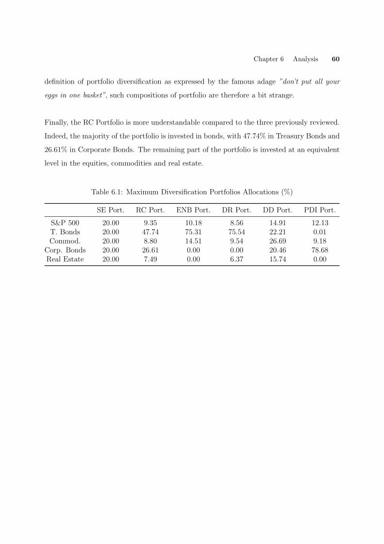
Chapter 6 Analysis 60
definition of portfolio diversification as expressed by the famous adage ”don’t put all your
eggs in one basket”, such compositions of portfolio are therefore a bit strange.
Finally, the RC Portfolio is more understandable compared to the three previously reviewed.
Indeed, the majority of the portfolio is invested in bonds, with 47.74% in Treasury Bonds and
26.61% in Corporate Bonds. The remaining part of the portfolio is invested at an equivalent
level in the equities, commodities and real estate.
Table 6.1: Maximum Diversification Portfolios Allocations (%)
SE Port. RC Port. ENB Port. DR Port. DD Port. PDI Port.
S&P 500 20.00 9.35 10.18 8.56 14.91 12.13T. Bonds 20.00 47.74 75.31 75.54 22.21 0.01Commod. 20.00 8.80 14.51 9.54 26.69 9.18
Corp. Bonds 20.00 26.61 0.00 0.00 20.46 78.68Real Estate 20.00 7.49 0.00 6.37 15.74 0.00

Chapter 6 Analysis 61
Figure 6.2: Maximum Diversification Portfolios

Chapter 6 Analysis 62
6.2.2 Results Analysis: Risk and Scores of Measures
As we have seen, some composition of portfolios can be di�cult to understand. However,
those allocations have been obtained by maximizing the di↵erent measures of diversification
so normally the portfolios should present high scores of measures and thus high degree of
diversification.
If we look at Table 6.2 and at the results of the maximum SE Portfolio, which is basi-
cally an Equally Weighted Portfolio (EWP), we can see it has indeed the maximum SE value
of 5, meaning that it represents a highly diversified portfolio from the perspective of the
weights concentration. But it doesn’t seem to be the case for the other measures. According
to the ENB and DR measures, the EWP is the least diversified portfolio of the group. And if
we look at the VaR and volatility level, it is clearly the riskiest portfolio of all. Moreover, the
corresponding Sharpe Ratio of the EWP is very low (0.4), which indicates that the portfolio
is not well risk-adjusted.
Table 6.2: Risk and Performance Statistics of the Maximum Diversification Portfolios
SE Port. RC Port. ENB Port. DR Port. DD Port. PDI Port.
Aver. Ret. (%) 6.38 5.81 4.89 5.32 5.71 6.27Variance (%) 0.72 0.20 0.19 0.17 0.69 0.25Volatility (%) 8.53 4.52 4.43 4.15 8.31 5.02
VaR5 1.95 1.03 1.01 0.95 1.90 1.15VaR1 2.75 1.46 1.43 1.34 2.68 1.62
Sharpe Ratio 0.40 1.28 1.10 1.28 0.69 1.25
SE 5.00 3.80 2.07 2.27 4.88 1.94RC Entropy 3.31 5.00 2.74 3.81 3.06 2.46
ENB 1.23 2.11 3.06 2.58 1.58 2.47DR 1.56 1.80 1.75 1.86 1.57 1.58DR2 2.43 3.24 3.06 3.46 2.46 2.50DD 0.37 0.43 0.42 0.45 0.37 0.37PDI 2.31 2.48 2.75 2.77 2.29 3.06

Chapter 6 Analysis 63
Another portfolio that presents a very high value for SE is the Diversification Delta Portfolio
(4.88). This is not very surprising since the DD is also an entropy-based measure, but it is
interesting to notice that the DD Portfolio has also an important level of risk with a volatility
equal to 8.31%. The two riskiest portfolios are thus those that are have been constructed
by minimizing the weights concentration (the maximization the entropy implies the mini-
mization of weights concentration). Therefore, following the observation of our results, it can
safely be said that the concentration criterion alone doesn’t seem to be adequate to construct
diversified portfolios.
Interesting also to notice the SE and DD portfolios have not a high diversification delta.
In fact, they have the lowest DD score with the PDI portfolio (0.37). This is quite surpris-
ing, especially for DD Portfolio because its construction is from the beginning based on the
maximization of the Diversification Delta. The portfolio with the highest DD score is the
one maximizing the Diversification Ratio of Choueifaty and Coignard (2008). Such portfolio
has actually be named ”Most Diversified Portfolio” by Choueifaty and Coignard and we can
see that it presents indeed some characteristics that we are looking for in a well-diversified
portfolio. First it is the less risky of the group with a volatility of 4.15 and it also shows the
highest Sharpe ratio (1.28). In addition, it has the highest score for most measures. The
only measure that doesn’t consider it as a well-diversified portfolio is the Shannon’s Entropy
(2.27), which is explained by the high percentage of its weights allocated to the Treasury
Bonds (75.54%). This extreme allocation is also traduced by a high percentage of risk con-
tributions in T-bills and a strong exposure to F4 as shown in Table B.4 and B.5 of Appendix
A. However, the portfolio seems to be e�ciently exposed to the di↵erent risk factors, as we
can see from the high scores of ENB, DR2 and PDI (2.58, 3.46 and 2.77 respectively).
The only portfolio having high scores in both entropy-based and risk-based measures is
the Risk Contribution Portfolio. The portfolio is constructed in a way that all asset classes
contributes to approximatively 20% of the total portfolio risk (this is not surprising given
that the portfolio maximizes Shannon’s entropy which uses the risk contributions instead of
Chapter 6 Analysis 64
the weights as inputs). The result is that the portfolio has a RC Entropy of 5 and shows a
good distribution of weights as depicted by a score of 3.80 in SE. Moreover, its risk profile is
very low with a volatility of 4.52% and it shares the highest Sharpe Ratio of 1.28 with the DR
Portfolio. It also shows an e�cient exposure to all the risk factors (ENB=2.11, DR2=3.24
and PDI=2.48). Therefore, as the latter, the Risk Contribution Portfolio seems to present
lots of characteristics of a well-diversified portfolio, from the concentration perspective as
well as from the risk-minimization perspective.
We have seen it, the portfolios constructed with PCA-based measures (ENB and PDI Port)
are extremely concentrated, especially in the bonds, Treasury or Corporates. As a result,
they show a poor score in SE, as well as in RC entropy which implies that the risk is not well
distributed between the asset classes. However, given the construction of the portfolios, their
expositions to the various sources of risk is e�cient according to their scores for ENB, DR2
and PDI. The volatilities of ENB and PDI portfolios are also quite low (4.43% and 5.02%
respectively) and the Sharpe Ratios high (1.10 and 1.25 respectively). We are thus here in
the case of a portfolio construction which minimizes the risk but has an allocation of weights
that is extremely concentrated, which doesn’t really reflect the basic idea of diversification.
Chapter 6 Analysis 65
6.2.3 Criteria of Diversification: Discussion
The results of our analysis have emphasized the point we have developed in the section 2.3:
some measures of diversification are only based on the risk minimization criterion and doesn’t
consider the weights concentration of a given portfolio. However, the only use of a measure
based on the entropy, like SE and DD, in order to quantify the diversification of a portfolio
doesn’t seem to be very e�cient. Indeed, our results have shown that a portfolio can have
weights that are well distributed between the di↵erent asset classes but have high volatility
level and thus a high risk profile. The Equally-Weighted portfolio created by maximizing the
Shannon’s entropy is a good example of that.
Moreover, following our analysis, the results we have obtained seem to indicate that the
Risk Contributions and the Diversification Ratio are more adequate measures in order to
quantify the diversification of a portfolio and also to create a well-diversified one. They are
indeed embodying the characteristics of diversification we have defined early on in Chapter
2 by providing high scores to portfolios which show a minimal risk profile but also small
concentrations in each asset classes.
Also, both measures verify some of the desirable properties that a measure of diversifica-
tion should have (section 2.2.2) like property 1, 2 and 3 as shown by Carmichael et al. (2015)
and Maillard, Roncalli and Teiletche (2009). However, since they don’t verify properties 4
and 5, we can be totally satisfied with the results they are providing. Also, the DR has been
critized by Lee (2011) and Taliaferro (2012) because the measure is not associated with a
clear objective function. Therefore, a portfolio constructed by maximizing the DR ”only has
desirable properties by accident” (Taliaferro (2012)).
The ENB and PDI have provided mitigates results because it doesn’t seem the measures
takes into account the concentration of the weights. As we have seen, the measures give
high scores, and thus indicate a high degree of diversification to portfolios that have weights

Chapter 6 Analysis 66
concentrated on few asset classes. Carmichael et al. (2015) have also shown the measures are
not e�cient to quantify diversification. Based on Embrechts et al. (1999), they have demon-
strated that ENB has two major shortcomings: ”it does not distinguish between negative and
positive correlation (and thus cannot incorporate the benefits arising from negative correla-
tion) and it can only be computed if portfolio risk is measured by its variance or volatility,
which are adequate measures of risk only in the unlikely case that asset returns are normally
distributed”.

Chapter 7
Conclusion and Further Research
This thesis wished to provide a thorough study of six measures of portfolio diversification:
the Shannon’s Entropy, the Diversification Delta, the Diversification Ratio, the Risk Contri-
butions, the Portfolio Diversification Index and the E↵ective Number of Bets. The results
were obtained on a database composed of five asset classes. The data were collected from
Bloomberg and are based on a weekly basis for the period from 29 December 1989 to 4 May
2018.
The introduction of the thesis presented the research question that we wanted to tackle.
In short, we wanted to study the ability of the di↵erent measures to quantify the diversifica-
tion level of a portfolio from the perspective of the risk minimization criterion and from the
weights concentration criterion. After reviewing the relevant theoretical content in chapters
2, 3 and 4, chapter 5 detailed the methodology followed and chapter 6 finished with the
presentation and discussion of the results.
In this conclusion, we will be focus on the implications of the results and we will answer
to the question that has been raised at the beginning of the thesis. We will end up with the
limitations of our works as well as suggestions for future research.
67

Chapter 7 Conclusion and Further Research 68
7.1 Implications of the Results
The main implication arising from our research is that it seems very di�cult to find a port-
folio which is well-diversified from the weights concentration perspective and also from the
risk minimization perspective at the same time. Indeed, the results we have obtained in our
analysis clearly show that if we want to obtain a portfolio with the minimum level of risk,
we have to do it at the cost of more concentration of the weights.
For example, based on our dataset, if we wanted to minimize the risk of a portfolio, it involved
more weights on the Treasury or Corporate Bonds. The Maximum Diversification Portfolios
constructed by maximization of the ENB, DR and PDI measures are good examples of that.
They concentrate more than 75% of their total weights in one of the two bonds asset class
to obtain a low risk profile. But such extreme allocations are not really in line with the
qualitative definition of diversification.
Another implication arising from our research is that the portfolios which have weights that
are (relatively) well distributed between the di↵erent asset classes are showing a riskiest
profile than the others. The SE and DD Portfolios reflect that pretty well. Moreover, it is
interesting to notice that their respective performances are not well risk-adjusted as repre-
sented by their Sharpe Ratio. This implication is quite surprising since lots of studies (we
can mention Bera and Park (2008), DeMiguel et al. (2005), Jorion (1985) as examples) have
been made on the subject of portfolios constructed with equal weights contribution and have
proven that such strategy (the 1/N asset allocation strategy to name it) delivers strong per-
formances. Therefore, we have decided to attribute the reason of such findings to the choice
of our database. Indeed, on one side we have the bonds which are characterized by a low
volatility and on the other side, we have the commodities, the equities and real estate which
are riskier asset classes.
Finally, the results of our study allow us to provide an answer to the research question
we have raised in chapter 1. Indeed, among the six di↵erent measures of portfolio diversifica-

Chapter 7 Conclusion and Further Research 69
tion we have analyzed, the one which seems to capture the most e�ciently the diversification
from the two criteria perspective is the risk contributions measure. It is the only one which
seems to consider the risk minimization criterion as well as of the weights concentration cri-
terion when judging the diversification level of a portfolio. Moreover, the Risk Contribution
Portfolio formed by the maximization of the measure represents a portfolio where the risk
is equally distributed between the di↵erent asset classes and where the weights are not too
concentrated, as depicted by the score of its Shannons Entropy.

Chapter 7 Conclusion and Further Research 70
7.2 Limitations and Suggestions for Further research
The results of our thesis need to be put into perspective. Indeed, as we have seen, the concept
of diversification is complex and hard to define in a financial context. In the framework of
our thesis, we have decided to compare the measures of diversification based on two criteria
but the choice of the latter can be challenged. Indeed, the absence of a common definition for
the concept of diversification in the literature makes it di�cult to perform a comparison of
di↵erent measures of diversification based on such imprecise definition. Moreover, the reality
of the market has proven that a large majority of academics and practitioners only consider
the risk minimization criterion when trying to diversify a portfolio. A clarification of the
concept is therefore something further research should put their attention on.
In addition, we choose to use the Shannon’s Entropy to analyze and quantify the concentra-
tions of a portfolio. However, such choice may not be the most appropriate. As a matter
of fact, several critics have been made about the use of Shannon’s Entropy as a measure of
portfolio diversification. For example, Carmichael et al. (2015) showed that the measure
doesn’t verify Property 2, 3, 4 and 5 that have been described in section 2.2.2. Therefore,
the use of another entropy in order to measure the diversification of a portfolio might be
necessary. The Rao’s Quadratic Entropy (Rao (1982)) has proved to be a strong candidate
by Carmichael et al. (2015). Such measure indeed verifies the five properties that are deemed
desirable for diversification measure and should be considered for further researches.
A last point would be about the choice of the variance/volatility and the VaR to measure
the risk of a portfolio. We have seen in section 2.1.2 that both variance and VaR can’t be
considered as coherent measures of risk. The variance violates the axiom of monotonicity
and the VaR does not obey the sub-additivity axiom. Therefore, it could be interesting to
analyze some measures of diversification which are considered as coherent measures of risk,
like the Conditional VaR (also called Expected Shortfall).
Bibliography
Ang, A., Hodrick, R., Xing, Y. and Zhang, Y. (2006). The Cross-Section of Volatility
and Expected Returns.Journal of Finance. Vol. 61, 259-299.
Anil K. Bera & Sung Y. Park (2008). Optimal Portfolio Diversification using the
Maximum Entropy Principle, Econometrics Reviews, Vol. 27:4-6, 4884-512
Artzner et al. (1999). Coherent Measures of Risk. Mathematical Finance, Vol.9, 203-228.
Barry, C.B. (1974). Portfolio Analysis under uncertain Means, Variances and Covari-
ances. Journal of Finance, Vol. 29, 515-522
Bawa, V.S., S.J. Brown and R.W. Klein. (1976) The E↵ect of Estimation Risk and
Optimal Portfolio Choice. Journal of Financial Economics, Vol. 3, 215-231
Best, M. J., and Grauer, R. R. (1991). On the Sensitivity of Mean-Variance E�cient
Portfolios to Changes in Asset Means: Some Analytical and Computational Results. The
Reviews od Financial Studies, Vol.4, 315-342.
Bloomfield, T., Leftwich, R., and Long, J. B. (1977). Portfolio strategies and perfor-
mance. Journal of Financial Economics, Vol.5(2), 201-218.
Campbell, L. (1966). Exponential Entropy as a Measure of Extent of a Distribution. Z.
Wahrscheinlichkeitstheorie verw., Vol.5, 217-225.
Chateauneuf, A. and Lakhnati, G. (2007). From Sure to Strong Diversification. Economic
Theory, Vol.32, 511-522.
Chateauneuf, A. and Tallon, J.-M. (2002). Diversification, Convex Preferences and
Non-empty Core in the Choquet Expected Utility Model. Economic Theory, Vol.19,
509-523.
71
Bibliography 72
Chopra, V.K. (1991). Mean-Variance Revisited: Near-Optimal Portfolios and Sensitivity
to Input Variations. Russel Research Commentary, 1991.
Chopra, V.K., Hensel, C.R., and Turner, A.L. (1991). Massaging Mean-Variance Inputs:
Returns from Alternative Global Investment Strategies in the 1980s. Management
Science, 1993.
Chopra, V.K., and Ziemba, W.T. (1993). The E↵ect of Errors in Means, Variances, and
Covariances on Optimal Portfolio Choice. Journal of Portfolio Management. Vol.19,
6-11.
Choueifaty,Y., and Coignard,Y.(2008).Toward maximum diversification. Journal of
Portfolio Management, Vol. 35(1), 4051.
Choueifaty, Y., Froidure, T. and Reynier, J. (2013). Properties of the Most Diversified
Portfolio. Journal of Investment Strategies, Vol.2(2), 49-70.
Deguest, R., Martellini, L., and Meucci, A. (2013). Risk Parity and Beyond -
From Asset Allocation to Risk Allocation Decisions. SSRN Electronic Journal, DOI:
10.2139/ssrn.2355778.
Dekel, E. (1989). Asset Demands Without the Independence Axiom. Econometrica, Vol.
57, 163-169.
De Giorgi, E. G., and Mahmoud, O. (2016). Diversification Preferences in the Theory of
Choice. Rivista di Matematica per le Scienze Economiche e Sociali, DOI: 10.1007/s10203-
016-0182-4.
DeMiguel et al. (2005). How Ine�cient is the 1/N Asset-Allocation Strategy? The
Review of Financial Studies, Vol. 22 (5), 1915-1953.
Dow Jones Equity All REIT Index. Retrieved from:
https://us.spindices.com/indices/equity/dow-jones-equity-all-reit-index-usd
Fabozzi, F. J. (2012). Encyclopedia of Financial Models. New York, NY: John Wiley
and Sons.
Fama, E. and French, K. (1992). The Cross-Section of Expected Returns.Journal of
Finance. Vol. 47, 427-465.
Fama, E. and French, K. (2003). The Capital Asset Pricing Model: Theory and Evidence.
Bibliography 73
Journal of Economic Perspectives. Vol.18, 25-46.
Fragkiskos, A. (2014). What is portfolio diversification? DOI:
http://dx.doi.org/10.2139/ssrn.2331475
Follmer, H., and Schied, A. (2010). Coherent and Convex Risk Measures. Encyclopedia
of Quantitative Finance, New York, NY: John Wiley and Sons, 355-363.
Follmer, H., and Schied, A. (2011). Stochastic Finance: An Introduction in Discrete
Time. Walter de Gruyter, Berlin.
Harris, B. (2006). Entropy. Encyclopedia of Statistical Sciences, Vol.3, 1992-1996.
Holton, G. A. (2004). Defining Risk. Financial Analysts Journal, Vol.60, 19-25.
Hua L and Xingsi L. 2003. A New Portfolio Model and Application. Operations Research
and Management Science, Vol.6, 83-86.
Investopedia. Treasury Bill - T-Bill. Retrieved from
http://www.investopedia.com/terms/t/treasurybill.asp.
Jobson, J.D., and Korkie, B. (1981) Putting Markowitz theory to work. The Journal of
Portfolio Management, Vol.7, 7074.
Jobson, J. D., and Korkie, B. (1980). Estimation for Markowitz e�cient portfolios.
Journal of the American Statistical Association, Vol. 75(371), 544-554.
Jorion, P. (1985). International portfolio diversification with estimation risk. J. Bus,
Vol.58, 259-278.
Kallberg, J.G, and Ziemba, W.T. (1984). Mis-specification in Portfolio Selection Prob-
lems. Risk and Capital: Lecture Notes in Economics and Mathematical Systems. New
York: Springer-Verlag, 1984.
Ke, J., and Zhang, C. (2008). Study on the optimization of portfolio based on entropy
theory and mean-variance model.IEEE International Conference on Service Operations
and Logistics, and Informatics. 2668-2672.
Klemkosky, R. and Martin, J. (1975). The e↵ect of Market Risk on Portfolio Diversifica-
tion. The Journal of Finance, Vol.30, 147-154.
Ledoit, O., and Wolf, M. (2004). Honey, I shrunk the sample covariance matrix. Journal
Portfolio Management Vol.30, 110-119.

Bibliography 74
Litner, J. (1965). The Valuation of Risk Assets and the Selection of Risky Investments in
Stock Portfolios and Capital Budgets. Review of Economics and Statistics. Vol.47, 13-37.
Ma, T., and Jagannathan, R. (2002). Risk Reduction in Large Portfolios: A Role for Port-
folio Weight Constraints. SSRN Electronic Journal. Vol.58, DOI: 10.2139/ssrn.293579.
Maillard, S., Roncalli, T., and Teiletche, J. (2009). On the properties of equally-weighted
risk contributions portfolios. SSRN Electronic Journal, DOI: 10.2139/ssrn.1271972
Markowitz, H. (1952). Portfolio Selection. Journal of Finance, Vol.7, 77-91.
Mehra, S.Y. and Hemming, R.S. (2003). Benefits of stock portfolio di-
versification. Retrieved from: http://www.aspecthuntley.com.au/af/news?xsl-
newsID=12&xtmlicensee=aspecthuntley
Merton, R. (1972). An Analytic Derivation of the E�cient Portfolio Frontier. The
Journal of Financial and Quantitative Analysis, Vol. 7, No. 4, 1851-1872.
Meucci, A. (2009). Managing Diversification. Risk, Vol.22(5), 74-79.
Michaud, R.O. (1989). The Markowitz optimization enigma: Is optimized optimal?.
Financial Analysts Journal, Vol.45, 3142
Morrison, D. F. (1990). Multivariate Statistical Methods, McGraw-Hill, New York.
Mossin, J. (1966). Equilibrium in a Capital Asset Market. Econometrica, Vol.34, No. 4,
768-783.
O’Toole, R. (2014). A Critical Review of Correlation-based Measures of Portfolio
Diversification. Presentation made at Northfield 27th Annual Research Conference.
Partovi, M.H., and Caputo, M. (2004). Principal Portfolios: Recasting the E�cient
Frontier. Economics Bulletin, Vol.7(3), 1-10.
Philippatos, G.C., and Wilson, C.J. (1972). Entropy, market risk, and the selection of
e�cient portfolios.Applied Economics, Vol.4, 209-220.
Reilly, F.K. and Brown, K.C. (2006). Investment analysis and portfolio management.
8th ed. Mason, OH: Thompson South-Western.
Riccardo, B. (2015) Risk Contribution and Measures of Portfolio Diversification. Master’s
Thesis from the Universit degli studi di Milano-Bicocca
Rich, R. and Tracy, J. (2006). The relationship between expected inflation, disagree-
Bibliography 75
ment, and uncertainty: evidence from matched point and density forecasts. Review of
Economics and Statistics, Vol.92, 200-207.
Risk Decomposed: Marginal Versus Risk Contributions. Retrieved from:
https://cssanalytics.wordpress.com/2012/07/10/risk-decomposed-marginal-versus-
risk-contributions/
S&P Global. (2016). [S&P U.S. Indices Methodology]. Retrieved from
https://us.spindices.com/documents/methodologies/methodology-sp-us-indices.pdf
Salazar et al. (2014). The Diversification Delta: A Di↵erent Perspective.
CIFR Paper, No.047, retrieved from: https://ssrn.com/abstract=2518705 or
http://dx.doi.org/10.2139/ssrn.2518705
Shannon, C.E., (1948). A Mathematical Theory of Communication. The Bell System
Technical Journal, Vol. 27, 379-423.
Sharpe, W.F. (1964). Capital Asset Prices: A Theory of Market Equilibrium under
Conditions of Risk. Journal of Finance. Vol.19, 425-442.
Schwartz, S. (2011). Risk Parity: Taking the Long View. I&PE, Retrieved from:
www.epe.com/risk-parity-taking-the-long-view/40025.article
Smith, D. (2006). A portfolio diversification index as a fund management instru-
ment. Cape Town: UCT. (Report - MBA) State Street Global Avisors (2018).
SPDR Bloomberg Barclays U.S. Corporate Bond UCITS ETF. Retrieved from:
https://ch.spdrs.com/library-content/public/SYB1%20GYfactsheeten.pdf
Wallis, K/ F. (2006). A Note on the Calculation of Entropy from Histograms. Departe-
ment of Economics, University of Warwick.
Zigrand, J. P. (2014). Systems and Systemic Risk in Fi-
nance and Economics. Systemic Risk Center, available on:
https://www.systemicrisk.ac.uk/sites/default/files/downloads/publications/sp-10.pdf
Appendix A
Summary Statistics and Results
76

Appendix A Summary Statistics and Results 77
Tab
leA.1:Ran
dom
lyGenerated
PortfoliosAllocations,Riskan
dPerform
ance
Statistics(%)
P1
P2
P3
P4
P5
P6
P7
P8
P9
P10
S&P500
24.02
3.42
4.67
4.39
20.79
27.86
60.96
29.20
17.08
16.08
T.Bon
ds
26.69
9.78
28.79
13,05
1.13
27.32
2.74
24.63
14.85
14.63
Com
mod
.3.74
19.22
28.39
28.34
26.92
14.42
23.91
11.24
29.81
21.22
Corp.Bon
ds
26.91
33.65
14.39
24.51
29.62
24.10
3.98
33.69
30.96
23.29
RealEstate
18.63
33.91
23.74
29.69
21.52
6.29
8.38
1.22
7.27
24.77
Aver.
Ret.(%
)7.18
6.59
5.53
5.96
6.37
6.29
7.17
6.35
5.42
6.46
Variance
(%)
0.55
0.81
0.74
0.91
0.98
0.49
1.69
0.40
0.67
0.81
Volatility(%
)7.40
9.00
8.62
9.54
9.89
6.99
13.01
6.36
8.18
8.99
VaR
51.69
2.05
1.97
2.18
2.25
1.60
2.97
1.45
1.87
2.05
VaR
12.39
2.90
2.78
3.08
3.19
2.26
4.20
2.05
2.64
2.90
SharpeRatio
0.57
0.73
0.64
0.62
0.64
0.90
0.55
1.00
0.66
0.72
SE
4.41
4.03
4.39
4.33
4.14
4.51
2.94
3.94
4.48
4.90
RC
Entropy
2.93
2.48
2.56
2.56
3.23
3.19
2.21
2.82
2.69
3.17
ENB
2.03
1.49
1.73
1.55
1.27
1.85
1.51
2.33
2.11
1.20
DR
1.47
1.50
1.54
1.50
1.51
1.60
1.30
1.60
1.55
1.54
DR
22.17
2.24
2.38
2.26
2.28
2.57
1.69
2.55
2.40
2.36
DD
0.33
0.35
0.35
0.34
0.35
0.38
0.25
0.38
0.36
0.36
PDI
2.32
2.19
2.24
2.23
2.30
2.36
1.91
2.40
2.27
2.28

Appendix A Summary Statistics and Results 78
Tab
leA.2:RiskCon
tribution
forRan
dom
Portfolios(%
)
P1
P2
P3
P4
P5
P6
P7
P8
P9
P10
S&P500
45.40
3.79
4.84
4.35
23.87
55.38
70.03
64.31
20.50
21.10
T.Bon
ds
1.91
0.24
0.48
0.01
-0.01
1.76
-0.12
2.99
0.44
0.06
Com
mod
.2.91
25.38
53.92
45.19
40.18
25.39
21.60
19.26
65.27
31.27
Corp.Bon
ds
6.43
4.83
1.67
2.47
2.60
5.62
0.06
11.24
4.68
2.71
RealEstate
43.35
65.76
39.08
47.98
33.36
11.85
8.43
2.19
9.12
44.86
Cumulative
(%)
100.00
100.00
100.00
100.00
100.00
100.00
100.00
100.00
100.00
100.00

Appendix A Summary Statistics and Results 79
Tab
leA.3:Diversification
Distribution
forRan
dom
Portfolios(%)
P1
P2
P3
P4
P5
P6
P7
P8
P9
P10
F1
78.87
89.85
86.03
89.99
95.05
81.95
86.03
68.62
74.89
96.08
F2
10.17
0.01
7.45
3.58
2.29
0.32
0.06
0.11
17.49
0.29
F3
1.40
5.12
2.54
3.34
0.09
7.76
13.83
14.42
0.95
0.13
F4
9.55
5.02
3.98
3.09
2.56
9.97
0.09
16.86
6.67
3.51
Cumulative
(%)
100.00
100.00
100.00
100.00
100.00
100.00
100.00
100.00
100.00
100.00

Appendix A Summary Statistics and Results 80
Table A.4: Risk Contribution for Maximum Diversification Portfolios (%)
SE Port. RC Port. ENB Port. DR Port. DD Port. PDI Port.
S&P 500 29.17 19.99 16.94 18.77 19.04 19.41T. Bonds 0.17 20.01 31.72 36.95 0.37 0.00Commod. 31.22 20.00 51.34 27.04 52.72 16.56
Corp. Bonds 2.56 20.01 0.00 0.00 2.69 64.03Real Estate 36.88 19.99 0.00 17.24 25.19 0.00
Cumulative (%) 100.00 100.00 100.00 100.00 100.00 100.00
Table A.5: Diversification Distribution for Maximum Diversification Portfolios (%)
SE Port. RC Port. ENB Port. DR Port. DD Port. PDI Port.
F1 95.45 54.89 38.56 52.31 87.74 30.34F2 0.37 0.19 18.85 1.71 7.48 1.70F3 0.15 0.09 2.01 0.05 0.01 3.28F4 4.03 44.82 40.58 45.93 4.76 64.68
Cumulative (%) 100.00 100.00 100.00 100.00 100.00 100.00

Place des Doyens, 1 bte L2.01.01, 1348 Louvain-la-Neuve, Belgique www.uclouvain.be/lsm