HAL Id: hal-00668277https://hal.archives-ouvertes.fr/hal-00668277v1Preprint submitted on 9 Feb 2012 (v1), last revised 6 May 2014 (v2)

HAL is a multi-disciplinary open accessarchive for the deposit and dissemination of sci-entific research documents, whether they are pub-lished or not. The documents may come fromteaching and research institutions in France orabroad, or from public or private research centers.

L’archive ouverte pluridisciplinaire HAL, estdestinée au dépôt et à la diffusion de documentsscientifiques de niveau recherche, publiés ou non,émanant des établissements d’enseignement et derecherche français ou étrangers, des laboratoirespublics ou privés.

Measurements of resonance frequencies of clarinet reedsand simulations

Pierre-André Taillard, Franck Laloë, Michel Gross, Jean-Pierre Dalmont, JeanKergomard

To cite this version:Pierre-André Taillard, Franck Laloë, Michel Gross, Jean-Pierre Dalmont, Jean Kergomard. Measure-ments of resonance frequencies of clarinet reeds and simulations. 2012. �hal-00668277v1�

Measurements of resonance frequencies of clarinet reeds and

simulations

Pierre-André Taillard1, Franck Laloë2, Michel Gross3,

Jean-Pierre Dalmont4 and Jean Kergomard5

1 Conservatoire de musique neuchâtelois,

Avenue Léopold-Robert 34; CH-2300 La Chaux-de-Fonds; Switzerland.2 Laboratoire Kastler Brossel – UMR 8552 Ecole Normale Supérieure,

UPMC, CNRS, 24 rue Lhomond; F-75231 Paris Cedex 05 ; France.3 Laboratoire Charles Coulomb - UMR 5221 CNRS-UM2, Université Montpellier,

II place Eugène Bataillon; F-34095 Montpellier ; France.4 Laboratoire d’Acoustique de l’Université du Maine - UMR CNRS 6613,

Université du Maine, F-72085 Le Mans; France.5 Laboratoire de Mécanique et d’Acoustique - CNRS, UPR 7051,

Aix-Marseille Univ, Centrale Marseille; F-13402 Marseille Cedex 20; France.

February 9, 2012

Abstract

A set of 55 clarinet reeds is observed by holography, collecting 2 series of measurementsmade under 2 different moisture contents, from which the resonance frequencies of the 15first modes are deduced. A statistical analysis of the results reveals good correlations, butalso significant differences between both series. Within a given series, flexural modes are notstrongly correlated. A Principal Component Analysis (PCA) shows that the measurementsof each series can be described with 3 factors capturing more than 90% of the variance:the first is linked with transverse modes, the second with flexural modes of high order andthe third with the first flexural mode. A forth factor is necessary to take into accountthe individual sensitivity to moisture content. Numerical 3D simulations are conducted byFinite Element Method, based on a given reed shape and an orthotropic model. A sensitivityanalysis revels that, besides the density, the theoretical frequencies depend mainly on 2parameters: EL and GLT . An approximate analytical formula is proposed to calculatethe resonance frequencies as a function of these 2 parameters. The discrepancy betweenthe observed frequencies and those calculated with the analytical formula suggests thatthe elastic moduli of the measured reeds are frequency dependent. A viscoelastic model isthen developed, whose parameters are computed as a linear combination from 4 orthogonalcomponents, using a standard least squares fitting procedure and leading to an objectivecharacterization of the material properties of the cane Arundo donax.

1 Introduction

Clarinettists experience every day the crucial importance of clarinet reeds for the quality ofsound. Their characterization is a real challenge for musicians who wish to obtain reeds that are

1

suited to their personal needs. The present paper address this complex field of research, but itsscope is restricted to the development of an objective method for a mechanical characterization ofsingle reeds of clarinet type. >From the shape and the resonance frequencies of each individualreed (measured with heterodyne holography), we intend to deduce the mechanical propertiesof the material composing it. A subsequent study should then examine how these mechanicalproperties are correlated with the musical properties of the reeds.

Natural materials, as wood or cane, are often orthotropic and exhibit a different stiffnessalong the grain (longitudinally) as in the others directions. The problem is then obviously mul-tidimensional. Nevertheless, reed makers classify their reeds by a single parameter: the nominalreed "strength" (also called "hardness"), in general from 1 to 5, which basically reflects the stiff-ness of the material (cane, Arundo donax L.), since all reeds of the same model have theoreticallythe same shape. The method of measurement is generally not publicized by manufacturers, butthis "strength" is probably related to the static Young modulus in the longitudinal direction EL.

"Static" (i.e. low frequency) measurements of the elastic parameters of cane are availablein the literature, for instance Spatz et al. [1]. A viscoelastic behavior has been reported inexperimental situations (see e.g. Marandas et al. [2], Ollivier [3] or Dalmont et al. [4]) and thisfact seems generally well accepted in wood sciences and biomechanics (for instance Speck et al.[5, 6]). Marandas et al. proposed a viscoplastic model of the wet reed. Viscoelastic behavior forcane was already demonstrated by Chevaux [7], Obataya et al. [8, 9, 10, 11] and Lord [12]. Theseauthors study only the viscoelasticity of the longitudinal Young modulus EL, leaving aside thefact that of the shear modulus in the longitudinal/tangential plane GLT . Furthermore, they giveno really representative statistics about the variability of the measured parameters.

Different authors (among them Casadonte [13, 14], Facchinetti et al. [15, 16] and Guimezanes[17]) modeled the clarinet reed by Finite Elements Method (FEM) and computed the first feweigenmodes. They chose appropriated values of the elastic parameters in the literature, ignor-ing however viscoelastic behavior. The goodness of fit between observations and model was ofsecondary importance, except for Guimezanes.

This latter author built a 2-D elastic model of the reed with longitudinally varying parameters.He fitted his model quite adequately with his observations (only 5 resonances were measured),but the fitted parameters seem not really plausible physically. His model didn’t respect theassumption of a radial monotonically decrease of stiffness from the outer side to the inner sideof the cane. Under such conditions, the frequency of the first resonance would increase incomparison to homogeneous material, and not decreased, as observed experimentally.

The observation of mechanical resonance frequencies can be achieved by different methods.The methods used by Chevaux, Obataya and Lord are destructive for the reed, which cannotbe used for further musical tests. On the contrary, holography is a convenient non-destructivemethod, the reed being excited by a loudspeaker. For instance Pinard et al. [18] measured withthis method the frequency of the 4 lowest resonances and focused their attention on the musicalproperties of the reeds.

The digital Fresnel holography method was used by Picart et al. [19, 20] and Mounier et al.[21] to measure high amplitude motion of a reed blown by an artificial mouth. Guimezanes [17]used a scanning vibrometer.

Recent technological developments provide very efficient and convenient measurements withholography, without having to manually identify the modes of resonance and to be satisfied witha single picture of their vibration: in a few minutes hundreds of holograms are acquired showingthe response of a reed for many frequencies. The temperature and the moisture content can beconsidered as constant during a measurement series1 The Sideband Digital Holography technique

1The significantly lower correlations between resonance frequencies (compared to our data) shows that it wasprobably not the case in Pinard’s study. This fact may also reflect an unprecise determination of the resonance

2

provides additional facilities (see 2.1.1).Generally, the physicist chooses a model in order to validate it by observations. In the present

study, the complexity of the problematic forced us to adopt the reverse attitude: We observethe mechanical behavior of clarinet reeds with a statistically representative sample and exploitafterward the statistical results for establishing a satisfactory mechanical model designed with aminimal number of parameters.

In section 2 the measurement method is presented. The experimental setup is described insection 2.1 and the method for observing resonance frequencies is detailed in 2.2. The resultsfor 55 reeds are given in section 3 (statistics, correlations and Principal Component Analysis(PCA)[22]).

In section 4, the development and the selection of a satisfactory mechanical model withminimal structure is described. First, a numerical analysis of the resonance frequencies of a reedassumed to be perfectly elastic is done by Finite Element Method (FEM), using the softwareCatia by Dassault systems, and a metamodel computing the resonance frequencies from elasticparameters is given in section 4.1. This allows to solve the inverse problem in a fast way. However,because the elastic model is not very satisfactory, viscoelasticity has to be introduced and someparameters are added to the model in section 4.2. The viscoelastic model has however too manydegrees of freedom, according to PCA. Consequently, the viscoelastic parameters of the model areassumed to be correlated and PCA indicates that these parameters can be probably reconstructedfrom 4 orthogonal components, as a linear combination, by multiple regression (section 4.3). Therelationships between the components and the viscoelastic parameters is given, and finally theresulting values for these parameters are discussed in section 4.4 and compared with the resultsof the literature.

2 Observations by Sideband Digital Holography

2.1 Experimental setup

2.1.1 Holographic setup

The experimental setup is shown schematically in Fig. 1. A laser beam, with wavelengthλ = 650 nm (angular frequency ωL) is split into a local oscillator beam (optical field ELO) andan illumination beam (EI); their angular frequencies ωLO and ωI are tuned by using two acousto-optic modulators (Bragg cells with a selection of the first order diffraction beam) AOM1 andAOM2: ωLO = ωL + ωAOM1 and ωI = ωL + ωAOM2, where ωAOM1,2 ≃ 2π × 80 MHz. The firstbeam (LO) is directed via a beam expander onto a CCD camera, while the second beam (I) isexpanded over the surface of the reed, which vibrates at frequency f . The light reflected by thereed (field E) is directed toward the CCD camera in order to interfere with the LO beam (ELO).4 phases were used (phase shifting digital holography) and we select the first sideband of thevibrating reed reflected light by adjusting ωAOM1,2 to fulfil the condition: ωAOM1 − ωAOM2 =2π(f + fCCD)/4, where fCCD is the CCD camera frame frequency. The complex hologramsignal H provided by each pixel of the camera, which is proportional to the sideband frequencycomponent of local complex field E, is obtained by 4-phases demodulation: H = (I0 −I2)+j(I1 −I3) where I0 . . . I3 are 4 consecutive intensity images digitally recorded by the CCD camera, andj2 = −1. From the complex hologram H , images of the reed vibration are reconstructed by astandard Fourier holographic reconstruction calculation [23]. These holographic reconstructedimages exhibit bright and dark interference fringes. Counting these fringes provides the amplitude

frequencies.

3

L

AOM1

AOM2

EL0

vibratingreed

+1

+1

0

0

BS

M

M

CCD

BE

EL

BE

E

EI

LS

Figure 1: Holographic setup. L: main laser; AOM1, AOM2: acousto-optic modulators; M:mirror; BS: beam splitter; BE: beam expander; CCD: CCD camera; LS: loudspeaker excitingthe clarinet reed through the bore of a clarinet mouthpiece at frequency f = ω/2π.

of vibration of the object (in the direction of the beam), which depends on the wavelength λ ofthe laser, and on the first Bessel function J1, for instance ±95nm for the first, ±770nm for the5th and ±1.6µm for the 10th maximum (bright fringes) [24, 25]2.

This method has 3 main advantages:(i) The time for data acquisition is very short, about 3 minutes for recording 184 holograms,

including holographic reconstruction.(ii) The signal to noise ratio is significantly better than with traditional technology, particu-

larly through the elimination of signal at zero frequency.(iii) The visualization of large-amplitude vibration (order of magnitude: 0.1 mm) is possible

by using high harmonics orders (up to several hundred times the excitation frequency).

2.1.2 Reed excitation

The reed was excited by a tweeter loudspeaker screwed onto an aluminium plate, connected to aclarinet mouthpiece. The lay of this mouthpiece was modified to be strictly flat. A plastic wedgeof uniform thickness has been inserted between the lay and the reed, longitudinally to the sameheight as the ligature (Vandoren Optimum), allowing free vibrations of the entire vamp (length:about 38 mm), see Fig. 1. This ensures precise boundary conditions, avoiding any dependenceto deformations of the reed. The repeatability of the longitudinal placing of the wedge and ofthe reed was ensured by a Claripatch ring [26].

This setup requires some comments:(i) The reed is excited exclusively through the bore of the mouthpiece.(ii) The pressure field in the chamber of the mouthpiece was not measured. Like for a real

instrument, the edges of the reed (protected by the walls of the chamber) are subject to a pressurefield, which is probably lower than the pressure acting on the rest of the vamp.

2The original notation from the cited paper is kept. This notation is only valid for this paragraph.

4

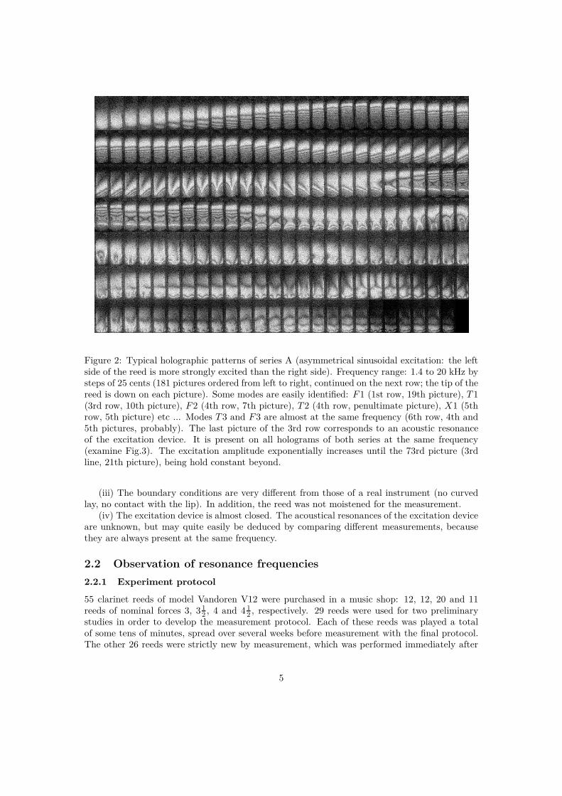
Figure 2: Typical holographic patterns of series A (asymmetrical sinusoidal excitation: the leftside of the reed is more strongly excited than the right side). Frequency range: 1.4 to 20 kHz bysteps of 25 cents (181 pictures ordered from left to right, continued on the next row; the tip of thereed is down on each picture). Some modes are easily identified: F1 (1st row, 19th picture), T 1(3rd row, 10th picture), F2 (4th row, 7th picture), T 2 (4th row, penultimate picture), X1 (5throw, 5th picture) etc ... Modes T 3 and F3 are almost at the same frequency (6th row, 4th and5th pictures, probably). The last picture of the 3rd row corresponds to an acoustic resonanceof the excitation device. It is present on all holograms of both series at the same frequency(examine Fig.3). The excitation amplitude exponentially increases until the 73rd picture (3rdline, 21th picture), being hold constant beyond.

(iii) The boundary conditions are very different from those of a real instrument (no curvedlay, no contact with the lip). In addition, the reed was not moistened for the measurement.

(iv) The excitation device is almost closed. The acoustical resonances of the excitation deviceare unknown, but may quite easily be deduced by comparing different measurements, becausethey are always present at the same frequency.

2.2 Observation of resonance frequencies

2.2.1 Experiment protocol

55 clarinet reeds of model Vandoren V12 were purchased in a music shop: 12, 12, 20 and 11reeds of nominal forces 3, 3 1

2 , 4 and 4 12 , respectively. 29 reeds were used for two preliminary

studies in order to develop the measurement protocol. Each of these reeds was played a totalof some tens of minutes, spread over several weeks before measurement with the final protocol.The other 26 reeds were strictly new by measurement, which was performed immediately after

5

Figure 3: Typical holographic patterns of series B (symmetrical sinusoidal excitation). Themodes X1 and T 3 cannot be distinguished anymore. Notice that T 1 is less marked than un-der asymmetrical excitation (for some reeds even difficult to identify) and that the pattern hasa significant flexural component, strongly dependent of the lateral placing of the reed on themouthpiece. Notice that the symmetry of the patterns near T 1 depends on the excitation fre-quency.

6

(a)

(b) (c)

Figure 4: (a) Flexural modes F1, F2, F3, F4 and F5. Side view. (b) transversal modes T 1, T 2,T 3, T 4, T 5. Front view. (c) Generic modes: X1, X2, X3, X4, X5 and X6. View from above.The intersections of nodal lines with the sides of the reed are symbolized by the blue dots.

package opening (for 21 of them with the new hermetically sealed package by Vandoren, ensuringa relative humidity between 45 and 70%, according to the manufacturer), without moisteningthe reed.

Each reed was subject to 2 series of measurements:

• Series A (asymmetrical excitation: see Fig.2): the right half of the mouthpiece chamberwas filled with modelling clay to ensure a good excitation of antisymmetrical modes. 184holograms were made ranging from 1.4 to 20 kHz (sinusoidal signal), by steps of 25 cents.The amplitude of the excitation signal was exponentially increased in the range 1.4 to 4kHz, from 0.5 to 16 V, then kept constant at 16 V up to 20 kHz. This crescendo limits theamplitude of vibration of the first two resonances of the reed. The temperature was notmeasured (about 20◦C).

• Series B (symmetrical excitation: see Fig.3): the modelling clay was removed. Theprotocol is otherwise identical to this of the first series. The reeds were inadvertentlyexposed during one night to the very dry and warm air from the optical laboratory betweenthe two series of measurements. The reeds lost between 2 and 4% of their mass. In whatfollows we try to interpret the influence of this fact. The temperature was around 23-25◦C.

2.2.2 Nomenclature of normal modes

Distinguishing 3 morphological classes, we classify the modes of a clarinet reed as follow : i) The“flexural” (or “bending”, or “longitudinal”) modes, listed below F , whose frequencies mainlydepend on the longitudinal Young modulus (EL) and polarized mainly in the z axis, ii) the“transversal” (or “ torsional”, or “twisting” ) modes, listed below T , mainly dependent on theshear modulus in the longitudinal / tangential plane (GLT ), and iii) the “generic” (or “mixed”)modes, listed below X , sensitive to both moduli EL and GLT (see Fig.4). A subclass of flexural

7

Figure 5: The clarinet reed: coordinates system. (a) top view, (b) front view, (c) side view. x,y, z: Cartesian axes of the object. L, T, R: axes of the orthotropic material (L: longitudinal,T: tangential, R: radial). In the software Catia used for the simulations, the orthotropic modelis Cartesian and not cylindrical. Therefore an exact equivalence between x, y, z, and L, T, Rrespectively can be assumed since we observed no important deviation between the direction ofthe grain and the axe of symmetry of the reed.

modes may be distinguished: the “lateral” modes (listed below L), polarized mainly in the y axis(see Fig. 5). These modes were not observed in our study.

The modes have been numbered after the order of increasing frequencies from a preliminarymodal analysis we performed. In our analysis, however, the identification of a mode is basedupon morphological criteria. As a matter of fact, the mode number and the order of observedfrequencies are not necessarily identical for all reeds.

Strictly speaking, the optical method only allows to observe the resonance frequencies of thereed and not the eigenfrequencies. Therefore the observed deformation patterns are a priori notidentical to the eigenmodes of the reed. Nevertheless in practice no major differences have befound between the computed eigenmodes (see section 4) and the observed or computed defor-mation for a forced asymmetrical excitation at the corresponding frequency. For this reason weuse the terminology “mode” for the maximum amplitude of the response of the reed to a forcedexcitation. This is somewhat abusive, because the small shift between the resonance frequenciesdue to damping and the eigenfrequencies computed by FEM, without damping, is ignored. Be-sides damping, the acoustic load is also able to shift the resonance frequencies. We assume thatthis discrepancy is approximatively the same for all reed.

2.2.3 Analysis of holograms; mode identification

More than 30000 holograms were made for this study and analyzed as follows: The picturewhere the number of interference fringes is locally maximum is determined. For some cases,we chose the hologram that is most similar to our numerical simulations (by Finite ElementMethod, see section 4) or to other holograms (see Fig.6). The holograms corresponding to anacoustical resonance of the system, present at the same frequency (4309 Hz) for all reeds, havebeen eliminated. The identification of the different patterns to those calculated by FEM wasoften quite simple. An exception have been encountered for F3 and T 3, whose frequencies wereoften so close that our identification is sometimes uncertain. More sophisticated techniqueswould certainly solve this problem. Notice that other boundary conditions (e.g. with clampingcloser to the tip of the reed) would also easily separate these two modes. The frequency of some

8

Figure 6: Qualitative comparison with FEM computation, and typical variability of the experi-mental results. (a) First row: Quasi-static pattern (at 605 Hz, with strong excitation by the LS).2nd to 5th row: Flexural modes F1, F2, F3 and F4. Leftmost column: numerical simulation ofeigenmodes by FEM. Columns 2 to 7: Arbitrary selection representing the observed variability(The first two rows correspond to the same selection of reeds). Notice the marked asymmetriesand the differences in the curvature of the interference fringes near the tip of the reed. (b) Rows1 to 5: transversal modes T 1, T 2, T 3, T 4 and T 5 (probably). Columns: see (a). (c) Rows 1to 6: Generic modes X1, X2, X3, X4, X5 and X6. The identification with X6 is sometimesunlikely. Columns: see (a).

higher modes could not always be measured, either because their frequency was beyond 20 kHz,or because their pattern could not be clearly identified.

3 Statistical analysis of resonance frequencies

4 flexural, 5 transversal, and 6 generic modes have been identified, namely all 15 first modes ofthe reed, excluding lateral modes. This number is significant, compared to the 4 modes detectedby Pinard et al. [18]. The 6th mode (L1) could not be identified, as it is a lateral mode (flexuralmode moving mainly in the y axis), not excited by our loudspeaker. We tried to observe it byrotating the mouthpiece to the side, without success. Notice that higher modes could probablybe identified using an ultrasonic loudspeaker.

3.1 Statistics

The statistics are displayed on Table 1. For 14 measurements of resonance frequencies of the twoseries, identification of the total number of reeds (55) have been done. For other measurements,identification has been done only for a part of this number. The value of the ratio of the standard

9

Series A Series BMode NA µ σ min max NB µ σ min max

F1 55 1996 77 1838 2154 55 1960 66 1812 2093T1 55 3377 132 3091 3676 55 3436 129 3136 3729F2 55 5130 161 4767 5669 55 4856 189 4435 5351T2 55 6108 261 5587 6939 55 6193 247 5669 7040X1 55 6869 198 6455 7458 45 6801 217 6363 7458T3 55 9571 500 8617 11014 54 9590 458 8742 11014F3 55 10146 419 9262 10857 55 9213 414 8372 10396X2 55 11521 387 10701 12187 54 11688 379 10857 13098X3 55 12294 368 11502 13482 11 12290 471 11839 13482T4 53 14011 756 12186 16503 54 14111 763 12186 16503F4 45 16784 552 15803 18524 54 15363 663 14079 17484X6 41 16984 972 15133 18793 30 16888 734 15577 18258X4 24 18497 518 17234 19067 23 17544 772 16033 19911X5 0 54 18896 501 17484 19911T5 0 14 19668 329 19067 19911

Total 658 668

Table 1: Observed resonance frequencies, sorted by frequency (in Hz). NA (resp. NB): Numberof identified pattern for each mode of series A (resp. B). µ: Mean value of the resonancefrequency, σ: Standard deviation, min: Minimum, max: Maximum. Total: total number ofidentified patterns for each series.

deviation σ to the mean value µ, i.e. the relative standard deviation, is found to be between2 and 5% (about 1/3 tone). If we admit Gaussian distribution for the measured frequencies,99% of the observations typically range about ±1 tone (±200 cents) around the mean value (i.e.µ ± 3σ), for all frequencies.

The identification of the mode X6 is uncertain: it seems to appear for frequencies lower thanthose of our simulations. Mode T 5 is on the limit of the range we studied: this explains thesmall value of the standard deviation.

Between series A and B, the flexural modes F1 to F4 lower their midrange, while the transver-sal modes slightly increase it. The difference between the two series probably lies mainly in thedrying of the reeds, and this seems to have a statistically significant effect. This is surprising,because drying decreases the density of the reed, and theoretically this should proportionallyincrease all frequencies. In addition, according to Obataya et al. [11], drying is expected toincrease E′

L (at least around 400 Hz), which should also increase the resonance frequencies.However Chevaux [7] observed that drying diminishes E′

L for material extracted from the innerside of the cane and augments slightly E′

L for material extracted nearer from the outer side (forcane suitable for oboe reeds), at least in the frequency range 100-500 Hz.

The hypothesis of an influence of the excitation method on the resonance frequencies seemsunlikely, as well as the hypotheses of a poor reproducibility of the position of the reed on themouthpiece between measurements or of the modification of the acoustic load, due to the mod-elling clay.

3.2 Correlations

Linear correlations have been computed between all possible couples of variables in a usual way(all the variables from Table 1, except X5 and T 5 of series A, i.e. 13 variables for series A and

10

15 for series B, plus the nominal reed strength). Results of series A for the mode F1 are denotedAF1, and similarly for the other results. The following 12 pairs have a correlation greater than0.9: AF1/BF13, AT1/BT1, AT2/BT2, AT3/AT4, AT3/BT3, AT3/BT4, BT3/BT4, AT4/BT3,BX1/BX3, AT4/BT4, BT4/BX6 and BX3/BX4. 54 pairs of variables have a correlation between0.8 and 0.9, 50 other pairs between 0.7 and 0.8 and 262 other pairs, below 0.7.

Between the two series, the correlation is excellent for corresponding transversal modes (T 1(i.e. AT1/BT1): 0.97, T 2: 0.97, T 3: 0.96 and T 4: 0.98), and generally good for correspondinggeneric modes (X1: 0.87, X2: 0.84, X3: 0.87 and X4: 0.55). For flexural modes, the correlationis good for F1 and progressively lower for increasing mode order (F1: 0.92, F2: 0.66, F3: 0.57and F4: 0.47).

Within the same series, on the contrary, there is a poor correlation between AF1 and allmeasurements of series A, and similarly for BF1 and series B. This is striking: the two bestcorrelated variables are AF2 and AX1 (0.73 and 0.49, respectively) for AF1 and BF2 and BT1(0.63 and 0.49, respectively) for BF1. Moreover, these correlations are quite low among allflexural modes: see Table 5. This fact is discussed in §4.4.

The nominal reed strength correlates at 0.7 with AT1 and AX4. We expected a bettercorrelation with F1 (only 0.6). This is surprising, since the reeds were probably sorted by aquasi-static bending method by the manufacturer. This would mean that the storage modulus ofEL at very low frequency is not well correlated with its value at the frequencies of the measuredresonances. The influence of density has also to be considered. However, Obataya et al. [9]observed a good correlation between density and EL. This point has to be investigated (see also§ C.4).

3.3 Principal component analysis

Principal Component Analysis (PCA) is mathematically defined as an orthogonal linear transfor-mation transforming the data to a new coordinate system, such that the greatest variance by anyprojection of the data comes to lie on the first coordinate (called the first principal component orfirst factor), the second greatest variance on the second coordinate, and so on [27]. TheoreticallyPCA is the optimum linear transform for given data in terms of least squares. PCA is basedupon the calculation of the eigenvalue decomposition of the covariance (or of the correlation)matrix (see e.g. [22]).

A PCA has been performed using the FACTOR module of SYSTAT [28]. The 14 variables(observed frequencies) presenting complete measurements for all reeds have been selected (allvariables having 55 identified pattern, NA or NB = 55, see Table 1). Frequencies are rated incents.

The 4 largest eigenvalues have been selected. They capture 91.2% of the total variance ofour sample (respectively 53.6%, 21.4%, 10.8% and 5.4% for each factor). A fifth factor wouldcapture only 2.5% variance more. The 14-dimensional data have been linearly projected onto a4-dimensional factor space.

The factor space can afterwards be orthogonally rotated, for instance for maximizing thecorrelations between rotated factors and observed variables. In the studied case, no a prioriknowledge about the orientation of the factor space is available. For an easy comparison, usingthe VARIMAX algorithm, we choose to maximize the correlations between rotated factors and allavailable variables (observed resonance frequencies and theoretical components from the modeldescribed hereafter in § 4.3.1).

3AF1/BF1 means AF1 versus BF1. The correlations are computed between AF 1[n] and BF 1[n], for n = 1 toN , where N = 55; missing observations are deleted.

11

factor1 factor2 factor3 factor4

AT2 0.973 0.054 0.078 -0.008BT2 0.953 0.055 -0.025 0.085AT3 0.898 0.198 -0.237 -0.032AX2 0.853 0.273 -0.073 -0.123AT1 0.776 0.017 0.577 0.087BT1 0.762 -0.033 0.541 0.177AX3 0.761 0.472 0.090 0.217AX1 0.740 0.451 0.356 0.115AF3 0.223 0.891 0.076 0.080AF2 0.143 0.791 0.519 0.064AF1 0.085 0.360 0.870 -0.141BF1 0.104 0.385 0.835 0.209BF3 0.059 0.596 0.050 0.755BF2 0.147 0.561 0.290 0.710e1 0.958 -0.080 0.105 0.005e2 0.059 0.969 0.082 0.098e3 -0.075 -0.073 0.971 0.042e4 -0.009 -0.081 -0.039 0.979

Table 2: Correlation (loadings) between rotated factors from PCA and : i) variables (measuredresonance frequencies) or ii) components from viscoelastic model (e[n], see § 4.3.1), for compar-ison, sorted in reverse order of magnitude. In bold: greater correlation for each variable.

We performed also a PCA separately for each measurement series (A and B: 9 and 5 variables,respectively). From series A we detected 3 important factors capturing 90.8% of the variance(56.9, 23.0, 11.0%, respectively). From series B we detected also 3 important factors capturing94.1% of the variance (54.0, 26.8, 13.3%, respectively). A 4th factor would capture only 3.6%more for series A and 3.4% for series B. One factor seemingly disappeared, compared with thePCA performed on both series. A hypothesis is that this factor is related to the hygrometricchange between the two series.

>From Table 2, we see that all transversal and generic modes are well correlated with factor1;factor2 correlates with high frequency flexural modes of both series (however notably better withthose of series A); factor3 well correlates with F1 of both series (and somewhat with other lowfrequency modes: AT1, BT1 and AF2), whereas factor4 correlates quite well with high frequencyflexural modes of series B.

3.4 Conclusions from the statistical analysis

Fifteen modes of vibration of the clarinet reed have been observed, while previous studies investi-gated 4 to 5 modes only [17, 18]. The observed resonance frequencies are often highly correlated,especially those among the “transversal” modes and, to a lesser extent, those among the “flex-ural” modes. The nominal reed strength is surprisingly better correlated with the frequenciesof “transversal” modes as with those of “flexural” modes. The flexural modes within the sameseries are poorly correlated.

A principal component analysis of the resonance frequencies identifies 4 main factors, cap-turing 91.2% of the variance of the sample. The data can therefore be reconstructed with 4uncorrelated factors only (error: RMSD = 21.8 cents, see Appendix C.2 and D). The effect ofhygrometric change between both measurement series can seemingly be described with 1 factor

12

only.These statistical facts offer a guidance for modeling appropriately the mechanics of the clarinet

reed.

4 Development and selection of a satisfactory mechanical

model

The determination of the mechanical parameters of a natural material is not an easy task. Thisrequires to determine for each axis of the orthotropic material the value of 3 parameters (Youngmodulus, shear modulus and Poisson’s ratio). These 9 parameters may exhibit viscoelastic be-havior, requiring theoretically for each one the fit of a viscoelastic model, such as the generallinear solid (also called Zener model or 3-parameter model, see [29, 30, 31, 32]). Other multidi-mensional viscoelastic models could be also considered. In order to fit a wide range of frequencies(more than 2 decades), a 4-parameter model with fractional derivative would be required [32].In addition, these parameters are known to be sensitive to moisture content. Moreover, the caneis not homogeneous. The stiffness varies in radial direction [7] and local irregularities may beimportant, as shown by J.-M. Heinrich [33].

We could not consider all these aspects in the present study. Our concern is to develop a modelwith a minimal number of components, that adequately reconstructs the observed resonancefrequencies of our reeds. We presume that these components offer an objective characterizationof the material composing each reed. A subsequent study should examine if these componentsare correlated with some musical qualities of the reeds. This could help the reed makers to gaina better control on their products.

This section is organized as follows: We first present results of FEM simulations (§ 4.1),assuming an elastic and orthotropic behavior of the reed (modeled in § 4.1.1). This helps toidentify the modes in experiments, and allows to obtain a fit formula (§ 4.1.3), ("metamodel"),for computing the 11 lower resonance frequencies with respect to two parameters only, EL andGLT , detected after a sensitivity analysis (§ 4.1.2). This, and the previous result of 4 factorsgiven by PCA, indicate that the orthotropic, elastic model is not sufficient to establish a satisfac-tory model with 2 degrees of freedom only. Therefore in the next subsection (§ 4.2) a viscoelasticmodel of cane is sought in order to find a fair reconstruction of the observed resonance frequenciesfor each reed and each series, after estimation of the coefficients in the model. The viscoelasticmodel (§ 4.2.2) has however too many degrees of freedom (12, for the 2 series of measurements,compared to the 4 factors detected by PCA), for solving adequately the inverse problem (§ 4.3).Multiple regression (see Appendix C for details) permits to regulate this drawback, introducingcorrelations among parameters and reducing the degrees of freedom to a number of 4. A hierar-chical structure can be introduced in the model, isolating the hygrometric component, bringingthe remaining 3 components to a common basis (§ 4.3.1), simplifying the problem (reduced toonly 9 "active" regression coefficients) and giving some insight in the structure of the data. Theresults are discussed in (§ 4.4).

4.1 Elastic model

4.1.1 Modeling the reed

The clarinet reed is defined in a Cartesian axis system x, y, z (see Fig. 5). The origin is located inthe bottom plane, at the tip of the reed. The material is defined as 3D orthotropic and assumed tobe homogeneous, whose longitudinal direction L is parallel to the x axis, the tangential direction

13

Coefficient F T X L All modesEL 0.4087 0.1053 0.1835 0.2093 0.2235

GLT 0.0140 0.2681 0.1962 0.1067 0.1575ET 0.0076 0.0976 0.0741 0.0166 0.0562

GLR 0.0438 0.0131 0.0257 0.0818 0.0341ER 0.0176 0.0120 0.0135 0.0662 0.0207

GT R 0.0046 0.0092 0.0077 0.0215 0.0091νT R 0.0015 0.0009 0.0015 0.0054 0.0019νLT 0.0018 -0.0031 0.0004 0.0007 -0.0001νLR 0.0009 0.0002 0.0005 0.0013 0.0007

Table 3: One-At-a-Time sensitivity study by FEM: Averaged ratio between relative change infrequency and relative change for each elastic coefficient (i.e. ±10%), sorted by decreasing orderof magnitude, for the first 16 eigenmodes. F : flexural modes (F1 to F4), T : transversal modes(T 1 to T 4), X : generic modes (X1 to X6), L: lateral modes (L1 and L2; these modes were notobserved in our study), All modes: averaged ratio over all modes. In bold: maximum absolutevalue for each coefficient of the orthotropic material: EL, ET and ER: Young moduli; νLT , νLR

and νT R: Poisson coefficients; GLT , GLR and GT R: shear moduli.

T parallel to the y axis and the radial direction R parallel to the z axis4.The dimensions in the xy plane are consistent with the measurements given by Facchinetti

et al. [16]. The heel of the reed is made out of a cylinder section, diameter 34.8 mm, maximumthickness 3.3 mm. The shape of the reed is defined in Appendix A.

During playing, the reed has two contact surfaces with the ligature. For the present simula-tions, the reed is clamped in the same way than for normal playing, on two rectangular surfaces23 × 1 mm, spaced laterally by 5 mm, 38.2 mm from the tip of the reed, simulating the contactsurfaces on the Vandoren Optimum ligature. However, unlike normal playing, the whole vampof the reed is free to vibrate (see Figure 1).

For the simulations, the “Generative Part Structural Analysis” module by Catia v.5.17 (Das-sault Technologies) is used, with mesh Octree3D, size 2 mm, absolute sag 0.1 mm, parabolictetrahedrons. The generated mesh involves 5927 points, allowing both a good accuracy and areasonable computing time (around 35 seconds).

4.1.2 Sensitivity analysis of elastic coefficients

An elastic, orthotropic and homogeneous material is defined by 9 independent coefficients: 3coefficients (Young modulus E, Poisson’s ratio ν and shear modulus G) for each axis (L: lon-gitudinal, T: tangential, R: radial). For selecting the most relevant parameters, we conducteda One-At-a-Time sensitivity analysis [34], varying each coefficient by ±10% and computing thefirst 16 modes, based on the following reference values: EL =14000 MPa, ET = ER = 480 MPa,νLT = νLR = νT R =0.22, GLT = 1100 MPa, GLR = GT R = 1200 MPa. The density ρ was setto 520 kg/m3, according to the estimation by Guimezanes [17]. The results are shown in Table3. Notice that EL and GLT plays a decisive role, while ET plays a marginal role and all otherparameters have an almost negligible influence on the resonance frequencies. As a consequence,the moduli EL and GLT are the variables retained in the model. The approximate value of ET

has been estimated according to the morphology of the patterns of higher order modes. Thisvalue is consistent with measurements given by Spatz et al. [1].

4Do not confuse the morphological mode classes L1, L2, T 1, T 2, T 3 and T 4 with the axes L and T of theorthotropic material.

14

Notice that these results show the validity of a 2D approach, the reed being modeled as athin plate. This should be used for further studies.

4.1.3 Metamodel approximating the resonance frequencies

The following analytic formula ("metamodel") predicts quickly and efficiently the resonance fre-quencies of a clamped/free clarinet reed. It was established in the following way: Frequenciesof the first 16 modes were computed by FEM, according to a network of 92 separate pairs ofvalues for EL and GLT , ranging from 8000 to 17000 MPa and 800 to 1700 MPa, respectively.The other elastic coefficients were held constant, according to the reference values cited above.For the range of simulation values, this arbitrary formula (developed by trial and error) providesa very good fit (generally better than ±5 cents, see Table 9). Expected resonance frequencies fare first found in cents (FC) from the note F6 (1396.9 Hz), and finally in Hz:

f(m, EL, GLT ) = 1396.9 × 2F C/1200, where (1)

FC = am,0 + am,1 Ep + am,2Gp + am,3 Ep Gp + am,4 E2p + am,5G2

p,

Ep = EL−0.66643 and Gp = GLT

0.7627.

The index m is the number of the mode defined in Appendix B, Table 9, where the values of thecoefficients am,q are given (EL and GLT are expressed in MPa).

The influence of the density is easy to predict: frequencies vary proportionally to ρ−1/2. Thecomputing cost of this metamodel is about 107 times lower than with FEM, largely simplifyingthe inverse problem.

4.2 Viscoelastic model

Equation (1) can be used to estimate the values of EL and GLT , providing a faithful reconstruc-tion of the observed resonance frequencies. Theoretically these values could be computed for anypair of modes, after their respective observed frequencies. Unfortunately, this method gives noconsistent results. A least squares fit is a more robust technique for such a computation. Thisleads however to systematic errors in the predicted frequencies: low-order modes are system-atically overestimated, while high-order modes are underestimated. This can be corrected byadjusting the coefficients am,0 (from Table 9), but this cannot explain the bad correlation amongflexural modes within the same series (see Table 5). According to the elastic model, these corre-lations should be in all cases greater than 0.998. A hypothesis for resolving this contradiction isthat the moduli are varying with the frequency in an individual way for each reed. We considerin this subsection a viscoelastic model, where EL and GLT are frequency dependent. This leadsto the addition of some parameters, which are to our mind more important that the other elasticcoefficients. The fit of such a model requires many observations at different frequencies, in orderto reduce the influence of measurements errors and of local irregularities in the structure of cane.

Alternative hypotheses could be considered in this context, as damping, acoustic load [16],local variations in stiffness or in density, local deviations in thickness, compared to the assumedtheoretical model. However, these hypotheses are probably unable to explain the hygrometric-induced individual variations we observed for each reed, thus our preference for the viscoelastichypothesis.

4.2.1 Some generalities about viscoelasticity

It is well known, that the stiffness of natural materials like wood or cane, similarly to that ofplastics, varies with the frequency of the applied stress and with the temperature. The material

15

E2E1

E3

Figure 7: Schematic representation of the standard linear solid: two springs E1, E2 and a dashpotE3.

is stiffer at low temperature and at high frequency. At low frequency or high temperaturethe material is almost perfectly elastic and reaches the rubbery modulus. At high frequencyor at low temperature the glassy modulus is reached; the material is almost perfectly elastic,also, but stiffer. At mid frequency or mid temperature, the apparent modulus (called storagemodulus, i.e. the real part of the complex Young modulus for this frequency) is between the twovalues. For a particular frequency, called relaxation frequency, the storage modulus is exactlyat the average of glassy and rubbery moduli. Around this frequency dissipation is maximum.Once the characteristic curve is known (for given temperature and different frequencies, or forgiven frequency and different temperatures), the Arrhenius equation5 offers usually an adequateestimate of the stiffness for any frequency and any temperature, within a quite broad range [29].

Considering viscoelasticity leads to complex modes with complex eigenfrequencies. Comparedto the non-dissipative, elastic case computed by FEM, the main consequence of viscoelasticity,besides dissipation, is that stress and stain are not in phase. For sake of simplicity, we limitthe computation to eigenfrequencies only, and assume that they depend on the storage modulionly (i.e. dissipation has a negligible influence). Having reduced the viscoelastic problem toan associated elastic one, the elastic solution may be used (see e.g. Ref. [29]). In order tocompute the resonance frequency ωr after an elastic model, according to Ref. [32], we admitthat E ≃ E′(ωr), where E′(ωr) is the real part of the complex modulus in the frequency domain.This hypothesis implies that the calculation of the eigenfrequencies from the values of the storagemodulus is done by an iteration procedure.

4.2.2 Choice of the viscoelastic model

In this section, a model of cane is considered, based on the standard viscoelastic solid, alsocalled Zener model or 3-parameter model (see e.g. Refs [29, 30, 31, 32]). The scheme of thestandard viscoelastic solid is presented on Fig.7, with two springs E1 and E2 and a dashpot E3

6.At low frequencies, E2 and E3 have practically no effect (the rubbery modulus E1 dominates).At high frequencies, E3 has practically no effect (the glassy modulus E1 + E2 dominates). Inthe frequency range near E2/(2πE3) the dissipation due to E3 is maximal and the apparent

5The shift in relaxation time is: Ln(shift) = Ea

R

(

1

T−

1

Tref

)

, where Ea is the activation energy, R is the

gas constant (8.314 J/K mol) and T and Tref the absolute temperatures in K. For instance, a shift of +10◦Cfrom a reference temperature of 20◦C decreases the relaxation time by 16%, if Ea is 13 kJ/mol.

6This notation allows to write the parameters of the model as a vector, as required by the computations, butunfortunately it hides the fact that the nature of E3 (dashpot) is physically different from E1 and E2 (springs).

16

modulus (storage modulus) is in the mid-range. The stress σ and the strain ε are related by theconstitutive equation:

σ + τ1σ = E1(ε + τ2ε) (2)

in which τ1 = E3/E2 is called the relaxation time and τ2 = E3(E1 + E2)/(E1E2) the retardationtime. E1 is called rubbery modulus and E1 + E2 glassy modulus. In harmonic regime, for anangular frequency ω, the Young modulus is complex:

E∗(ω) = E1 + E2 − E22

E2 + jωE3= E1 + E2 +

−E2 + jωE3

1 + (ωE3/E2)2 (3)

The second formulation separates the real part (E′(ω): storage modulus) and the imaginary part(E′′(ω): loss modulus) of E∗(ω). The storage modulus can thus be written as:

E′(ω) = E1 + E2 − E32

E22 + ω2E2

3

= E11 + ω2τ1τ2

1 + ω2τ21

. (4)

Notice the properties:

E′(0) = E1 ; E′(1/τ1) = E1 + E2/2

E′(∞) = E1 + E2 ;∂E′

∂ω

( 1

τ1

)

=E3

2.

This model is applied to both moduli EL and GLT . For sake of simplicity, the parameters aredenoted E1, E2, E3, and G1, G2, G3, and the storage moduli given by Equation (4) E′(ω) andG′(ω), respectively. Therefore for each reed (and each series), the model requires 6 parametersinstead of 2 (while experiments gave 4 main factors only for the whole set of results).

>From the knowledge of the 6 parameters, the resonance frequencies can be deduced by aniteration procedure. For each mode the starting point of the iteration is the mean value f (0) ofthe experimental resonance frequency (see Table 1), then the storage moduli are deduced fromEquation (4), then a new value f (1) by using Equation (1), etc... The convergence of the iterationmethod is fast, actually one iteration is enough. This can be understood by the fact that thederivative of the iterated function is small (notice that the two first rows of Table 3 correspondto the derivative of EL and GLT with respect to frequency). If we give an arbitrary value, forinstance f (0) = 6000, one iteration more is required for a comparable precision. In all hypotheses(see Appendix C.6), we used one iteration only. This procedure allows the determination of f(m)from the coefficients E1, E2, E3, G1, G2, G3 for a given reed and a given series.

4.3 Inverse problem: selecting a satisfactory model

In order to solve the inverse problem for each reed (and each series), we use a classical MeanSquared Deviation method, from the experimental values of the 11 resonance frequencies listedin Table 9. We tested different hypotheses to establish a satisfactory model. The details canbe found in Appendix C. A constant value elastic model (hypothesis H1) or 2 parameter elasticmodel (hypothesis H2) are not sufficient, whereas a 12 parameter viscoelastic model (H9) con-ducts sometimes to non-physical results (negative rubbery modulus, for instance). For respectingthe assumption of 4 independent parameters (as detected by PCA), correlations among the vis-coelastic parameters have to be introduced, as a linear combination of 4 orthogonal components.These 4 components are very similar to the 4 factors computed by the PCA, but, because ofthe non-linear nature of Equations (1 and 4), a small deviation is inevitable for optimal results.

17

100 1 000 10 000 100 0006000

8000

10 000

12 000

14 000

16 000

18 000HaL

HbLHcL

HdL

Figure 8: Hypothesis H4: plot of the storage moduli E′

L(ω) and G′

LT (ω) [in MPa], after Equations(4 to 7), computed for the mean value of all reeds. (a): E′

L series A, (b): E′

L series B, (c): G′

LT

series A and (d): G′

LT series B. For G′

LT , the moduli are multiplied by 10. The abscissa of therelaxation frequencies [in Hz] are denoted by dashed lines (series A) and dotted lines (series B).The corresponding numerical values are listed in Tables 6 and 7. Only the portions of the curvesbetween 2 and 18 kHz could be fitted adequately. The curves outside this range are purelyhypothetical: we have no measurements.

Factors and components are consequently strongly correlated (>0.95, see Table 2). A full linearmodel with 60 independent coefficients (H7) is not necessary, because many coefficients are verysmall. A 9 coefficient linear model (H4) is very satisfactory and we describe it hereafter.

The RMSD (Root Mean Square Deviation: see Appendix C.2) is found to be 30.4 cents forH4, very close to 29.8 cents for H5 with 9 coefficients more. Moreover the standard deviationof the residuals for hypothesis H4 (and also hypothesis H5) varies very few over the differentresonance frequencies (all around 30 cents).

For sure, the quality of fit cannot be considered as a perfect and definitive proof that ourmodels reflect the true values of the corresponding storage moduli. The influence of some missingparameters in the model should be examined (for instance differences in thickness between reeds,non constant modulus ET , non constant density ρ or radial variation of EL). Anyways, thepresented models reflect real mechanical differences between the reeds, very similar to thosedetected objectively by the PCA.

4.3.1 Description of a satisfactory 9-coefficients model (hypothesis H4)

This model is designed so that no coefficient can be removed without impacting notably thequality of fit. It can be thought as the minimal structure allowing an adequate reconstructionof the observed resonance frequencies, in conjunction with the viscoelastic model Equation (4)and the metamodel Equation (1). This minimal structure makes the model more robust againstmeasurements errors, but it introduces probably some bias.

As a first step, our concern is to eliminate the influence of the moisture content and bringboth series of measurement to a common basis. If e1[n], e2[n], e3[n] and e4[n] are the 4 indepen-dent components characterizing the mechanical properties of the reed n (these components areconditioned similarly to PCA as orthogonal factors: mean 0, standard deviation 1 and intercor-

18

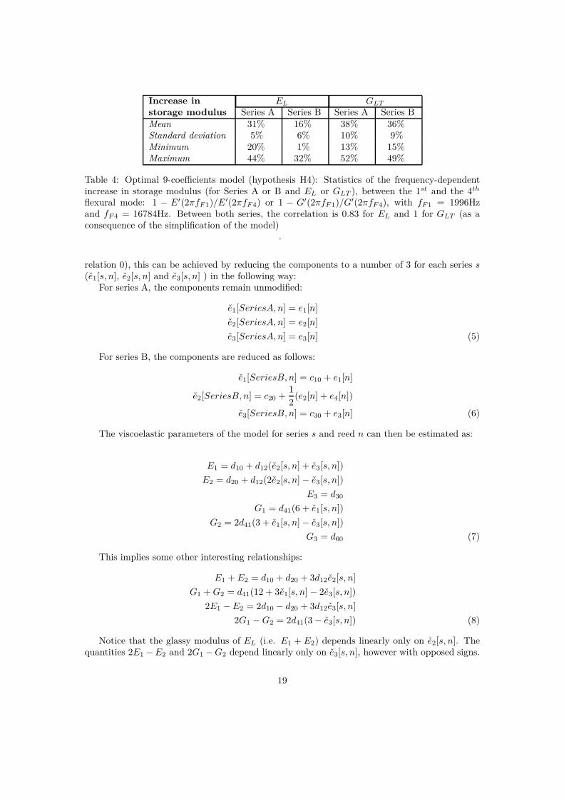
Increase in EL GLT

storage modulus Series A Series B Series A Series B

Mean 31% 16% 38% 36%Standard deviation 5% 6% 10% 9%Minimum 20% 1% 13% 15%Maximum 44% 32% 52% 49%

Table 4: Optimal 9-coefficients model (hypothesis H4): Statistics of the frequency-dependentincrease in storage modulus (for Series A or B and EL or GLT ), between the 1st and the 4th

flexural mode: 1 − E′(2πfF 1)/E′(2πfF 4) or 1 − G′(2πfF 1)/G′(2πfF 4), with fF 1 = 1996Hzand fF 4 = 16784Hz. Between both series, the correlation is 0.83 for EL and 1 for GLT (as aconsequence of the simplification of the model)

.

relation 0), this can be achieved by reducing the components to a number of 3 for each series s(e1[s, n], e2[s, n] and e3[s, n] ) in the following way:

For series A, the components remain unmodified:

e1[SeriesA, n] = e1[n]

e2[SeriesA, n] = e2[n]

e3[SeriesA, n] = e3[n] (5)

For series B, the components are reduced as follows:

e1[SeriesB, n] = c10 + e1[n]

e2[SeriesB, n] = c20 +1

2(e2[n] + e4[n])

e3[SeriesB, n] = c30 + e3[n] (6)

The viscoelastic parameters of the model for series s and reed n can then be estimated as:

E1 = d10 + d12(e2[s, n] + e3[s, n])

E2 = d20 + d12(2e2[s, n] − e3[s, n])

E3 = d30

G1 = d41(6 + e1[s, n])

G2 = 2d41(3 + e1[s, n] − e3[s, n])

G3 = d60 (7)

This implies some other interesting relationships:

E1 + E2 = d10 + d20 + 3d12e2[s, n]

G1 + G2 = d41(12 + 3e1[s, n] − 2e3[s, n])

2E1 − E2 = 2d10 − d20 + 3d12e3[s, n]

2G1 − G2 = 2d41(3 − e3[s, n]) (8)

Notice that the glassy modulus of EL (i.e. E1 + E2) depends linearly only on e2[s, n]. Thequantities 2E1 − E2 and 2G1 − G2 depend linearly only on e3[s, n], however with opposed signs.

19

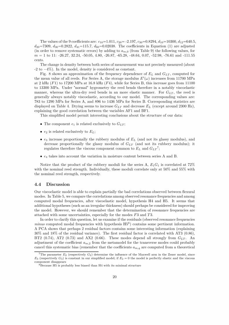
The values of the 9 coefficients are: c10=1.011, c20= -2.197, c30=0.8294, d10=10300, d12=640.5,d20=7309, d30=0.2822, d41=115.7, d60=0.02038. The coefficients in Equation (1) are adjusted(in order to remove systematic errors) by adding to am,0 (from Table 9) the following values, form = 1 to 11: -26.27, 32.24, -50.05, 4.80, -26.87, -65.28, -48.64, 0.07, -52.98, -76.61 and -111.55cents.

The change in density between both series of measurement was not precisely measured (about-2 to −4%). In the model, density is considered as constant.

Fig. 8 shows an approximation of the frequency dependence of EL and GLT , computed forthe mean value of all reeds. For Series A, the storage modulus E′(ω) increases from 11700 MPaat 2 kHz (F1) to 17200 MPa at 16.8 kHz (F4), while for Series B, this increase goes from 11100to 13300 MPa. Under "normal" hygrometry the reed bends therefore in a notably viscoelasticmanner, whereas the ultra-dry reed bends in an more elastic manner. For GLT , the reed isgenerally always notably viscoelastic, according to our model. The corresponding values are:783 to 1290 MPa for Series A, and 896 to 1436 MPa for Series B. Corresponding statistics aredisplayed on Table 4. Drying seems to increase GLT and decrease EL (except around 2300 Hz),explaining the good correlation between the variables AF1 and BF1.

This simplified model permit interesting conclusions about the structure of our data:

• The component e1 is related exclusively to GLT ;

• e2 is related exclusively to EL;

• e3 increase proportionally the rubbery modulus of EL (and not its glassy modulus), anddecrease proportionally the glassy modulus of GLT (and not its rubbery modulus); itregulates therefore the viscous component common to EL and GLT

7;

• e4 takes into account the variation in moisture content between series A and B.

Notice that the product of the rubbery moduli for the series A, E1G1 is correlated at 72%with the nominal reed strength. Individually, these moduli correlate only at 50% and 55% withthe nominal reed strength, respectively.

4.4 Discussion

Our viscoelastic model is able to explain partially the bad correlations observed between flexuralmodes. In Table 5, we compare the correlations among observed resonance frequencies and amongcomputed modal frequencies, after viscoelastic model, hypothesis H4 and H5. It seems thatadditional hypotheses (such as an irregular thickness) should perhaps be considered for improvingthe model. However, we should remember that the determination of resonance frequencies areattached with some uncertainties, especially for the modes F3 and T 3.

In order to clarify this question, let us examine if the residuals (observed resonance frequenciesminus computed modal frequencies with hypothesis H58) contains some pertinent information.A PCA shows that perhaps 2 residual factors contains some interesting information (explaining30% and 18% of the residual variance). The first residual factor is correlated with AT3 (0.86),BT2 (0.74), AT2 (0.73) and AX2 (0.66). These modes depend all strongly from GLT . Anadjustment of the coefficient am,2 from the metamodel for the transverse modes could probablycancel this systematic bias (remember that the coefficients am,q are computed from a theoretical

7The parameter E2 (respectively G2) determine the influence of the Maxwell arm in the Zener model, sinceE3 (respectively G3) is constant in our simplified model; if E2 = 0 the model is perfectly elastic and the viscouscomponent disappears

8Because H5 is probably less biased than H4 with its minimal structure

20

Model Mode AF1 AF2 AF3 BF1 BF2 BF3F2 0.73 0.63

observations F3 0.34 0.75 0.43 0.84F4 0.28 0.65 0.74 0.00 0.43 0.45F2 0.93 0.79

H4 F3 0.69 0.90 0.62 0.97F4 0.56 0.81 0.98 0.36 0.82 0.91F2 0.90 0.69

H5 F3 0.57 0.87 0.52 0.98F4 0.43 0.77 0.98 0.26 0.84 0.92

Table 5: Correlations of resonance frequencies between flexural modes within the same series,after observations and viscoelastic models H4 and H5. AF1, AF2, AF3, BF1, BF2 and BF3:correlations with modal frequencies F1, F2 and F3 within series A or series B. Lines: corre-sponding flexural mode between which the correlations are computed.

model, which is probably also biased). Indeed, an increase of 14, 21, 16 and 11% of this coefficientaffecting the modes T 1, T 2, T 3 and T 4 drop the RMSD from 29.8 to 28.5 cents. The secondresidual factor is correlated with AF1 (0.36), AF2 (0.29), AT2 (−0.29), BF1 (0.28) and BT1(−0.23). This reveals probably a competition between flexural and transversal modes when fittingthe model. The bias comes probably from the coefficient am,1, regulating the linear dependanceto EL in the metamodel. Adjusting the coefficients am,1 for all modes and the coefficients am,2

for all transverse and generic modes drop the RMSD down to 26.2 cents, reaching practicallythe size of the measurement steps (25 cents). The adjustments of am,1 are very small for theflexural modes F1 to F4: -6, 1, 6 and 1%.

This shows that the most important bias depends linearly from the 2 most important pa-rameters (EL and GLT ) of our FEM computations. No supplementary parameter is requireduntil this bias is removed (theoretically down to a RMSD of 21.8 cents, according to H10). Forhypothesis H4, the same linear adjustment of the metamodel let drop the RMSD from 30.4down to 27.0 cents.

A comparison with results by other authors is difficult or even quite impossible, because ofthe disparate structure of the measurements. Such a comparison requires the reconstruction ofthe measurement data (when possible), the fit of a viscoelastic model or the extrapolation of thevalues, in order to reach the frequency and temperature range of our measurements. The validityof such a highly speculative task is questionable. For the storage modulus E′

L, the reconstructedvalues from other authors fall all in the range around the mean of our measurements ±3 timesthe standard deviation, however most of the time in the lower range. This shows probably thatthe selected value for the density ρ was somewhat too high. No representative statistics areavailable by the other authors.

The most important disagreement, compared with our model (hypotheses H4 and H5), isabout the relaxation frequency. The explanation is probably because the studied frequencyrange was not same. For GLT , we found no viscoelastic measurements by other authors. Ourresults are summarized in Tables 6 and 7. For E′

L, between hypotheses H4 and H5, fr and E′

L at4 kHz agree well, whereas E1 and E2 diverge by about 1-2 SD. This divergence comes becausethe observed frequency range was not broad enough. For the shear modulus, G1 and G2 are ingood agreement for both hypotheses (and consequently fr and G′

L at 4 kHz also).Our model is valid only for "ambient dry" reeds (since the ultra-dry conditioning was not

controlled), in a frequency range which should not exceed one decade. We checked that a

21

Model Storage Young modulus E′

L(ω) at about 20◦CE1 [MPa] E2 [MPa] fr [Hz] E′

L at 4 kHz

Hypothesis H4, series A10300,SD 906

7309,SD 1432

4123,SD 808

13781,SD 897

Hypothesis H5, series A9377,SD 844

8336,SD 1552

4027,SD 750

13449,SD 839

Hypothesis H4, series B9423,SD 784

3964,SD 1109

2236,SD 626

12338,SD 885

Hypothesis H5, series B7844,SD 753

5459,SD 1217

1947,SD 434

12168,SD 882

Table 6: Summary of our results for hypotheses H4 and H5 about the viscoelastic behavior ofthe longitudinal Young modulus EL in cane. E1, E2 and fr (relaxation frequency): parametersfrom Zener model. E′

L at 4 kHz : storage modulus at 4 kHz [in MPa]. SD: standard deviation(the value preceding SD is the average). The model is valid only between 2 and 18 kHz.

Model Storage Shear modulus G′

LT (ω) at about 20◦CG1 [MPa] G2 [MPa] fr [Hz] G′

LT at 4 kHz

Hypothesis H4, series A 694, SD 116 694, SD 3275420,SD 2555

926, SD 102

Hypothesis H5, series A 752, SD 119 628, SD 3286310,SD 3296

924, SD 105

Hypothesis H4, series B 811, SD 116 736, SD 3275749,SD 2555

1042, SD 99

Hypothesis H5, series B 774, SD 119 769, SD 3285622,SD 2401

1022, SD 103

Table 7: Summary of our results for hypotheses H4 and H5 about the viscoelastic behavior of theshear modulus in longitudinal / tangential plane GLT in cane. G′

LT at 4 kHz: storage modulusat 4 kHz. Same structure as Table 6. The model is valid only between 2 and 18 kHz.

22

fractional derivative model after Gaul et al. [32] is not necessary in our narrow frequency range.Such models are however really efficient to cover a broad frequency range. For instance, thedata by Lord for dry material [12] could be fitted very well (E0 = 8108 MPa, E1 = 2964 MPa,p = 0.298 MPa·sα, α = 0.546). Notice that the order of the derivative (α) is 1 in our viscoelasticmodel.

5 Conclusion

The main results from the statistical analysis are discussed in §3.4. >From these results it waspossible to establish a satisfactory numerical model, selecting the most important parametersdescribing the mechanical behavior of a reed.

A sensitivity analysis by FEM calculation assuming an orthotropic, elastic material has beenconducted, and showed that the longitudinal Young modulus EL and the longitudinal / trans-verse shear modulus GLT play a leading role. An efficient metamodel could be developed toapproximate the resonance frequencies of a clarinet reed from these two moduli. In order toimprove the model, we consider the hypothesis of frequency dependent moduli, introducing ad-ditional degrees of freedom. A reconstruction of the observed resonance frequencies can thenbe achieved with a good accuracy, estimating for each reed only 4 components, from which theparameters of a viscoelastic model are computed as a linear combination. The selected model(after hypothesis H4) is probably slightly biased, but it is more robust against measurementerrors than more refined models.

Table 2 shows that these components are highly correlated to the factors computed by PCA(0.96 to 0.98). A multiple regression confirmed the data structure detected with the viscoelasticmodel.

The proposed method allows the determination of 3 mechanical parameters characterizingthe material composing each reed, with a single series of measure, using Equations (1, 4 and7). The reed should be conditioned with a relative humidity corresponding to the one ensuredby the hermetically sealed package by Vandoren (about 55%). The forth parameter cannot bedetermined in a reproducible way, since the exposition of the reeds to the ultra-dry air of theoptical laboratory was not controlled. The same protocol and the same viscoelastic model canbe used for other kinds of single reeds (bass clarinet, saxophone). Only the coefficients of Table9 have to be recomputed after a FEM simulation of the corresponding reed shape.

Despite the fact that the eigenmodes of higher order probably play no important role in theacoustics of the clarinet, the present study shows that they reveal the inner structure of thematerial building the tip of the reed, so a new step could be done for an objective mechanicalcharacterization of the clarinet reed.

Acknowledgments

We express gratitude for the financial aid from association DEPHY of the "département dephysique de l’ENS", and to Fadwa Joud for her help during the experiments. The Haute-EcoleARC (Neuchâtel, Berne, Jura) provided the software for simulation and calculation, and offeredhelpful instructions. The Conservatoire neuchâtelois partially supported this study for nearly3 years. We also thank Bruno Gazengel, Morvan Ouisse and Emmanuel Foltête for fruitfuldiscussions.

APPENDICES

23

A Defining the shape of the reed

x [mm]s0 [mm]

y=0 mms1 [mm]y=4mm

s2 [mm]y=6mm

0 0.074 0.080 0.0425 0.343 0.293 0.197

10 0.648 0.542 0.37715 1.047 0.847 0.57120 1.451 1.135 0.74525 1.926 1.527 1.07830 2.540 2.084 1.58935 3.351 2.817 2.256

Table 8: Network of points for interpolating the thickness of the vamp. See explanations in thetext.

The thickness of the vamp at point (x, y) is interpolated as follows: first, we interpolate 3points at y=0, 4 and 6mm, with 3 cubic splines, after Table 8. These three points (s0(x), s1(x)and s2(x)) define a biquadratic polynomial:

vamp(x, y) = p0(x) + p1(x) y2 + p2(x) y4

with p0(x) = s0(x), p1(x) = (−65 s0(x)+81 s1(x)−16 s2(x))/720 and p2(x) = (5 s0(x)−9 s1(x)+4 s2(x))/2880, allowing an interpolation on the y axis. The network of points above was estimatedusing a least squares fit, based on a network of 12 × 24 thickness measurements, achieved with adial indicator and a coordinates-measuring table (estimated accuracy: ±5µm in z, ±50µm in xand y). We measured twenty reeds and select a particularly symmetrical one as reference. Thismethod allows the reconstruction of the measurement network with an accuracy of ±10µm.

The thickness of the heel is defined to be :

heel(y) = −14.1 +√

17.42 − y2

The contour of the reed in the xy-plane is defined by:

contour(x) =

0 x < 0 or x ≥ 67.5√

(24.4 − x)x x < 1.13196

4.08044 +√

−5.31 + 6.8x − x2 x < 2.9466126340 − 11

900 x x < 67.5

The thickness of the reed at point (x, y) is defined by:

thickness(x, y) =

{

min[heel(y), vamp(x, y)] Abs(y) < contour(x)

0 otherwise

B Coefficients of the metamodel

24

mode m am,0 am,1 am,2 am,3 am,4 am,5 δ− δ+F1 1 2334.56 -1165877 0.2763 -21.99 145883795 -0.000324 -2 4T 1 2 1481.70 -642027 5.0725 569.69 83451520 -0.005886 -3 3F2 3 3651.79 -1060625 0.7082 -123.77 130061359 -0.000786 -2 5T 2 4 2403.82 -493591 3.8130 501.70 64716271 -0.003741 -9 5X1 5 3153.73 -822597 3.1425 604.29 105032670 -0.003785 -3 4F3 6 4669.87 -1009348 0.7623 -101.18 122741172 -0.000877 -3 6T 3 7 3015.77 -275531 3.5285 250.00 29933670 -0.003016 -2 1X2 8 3874.44 -633268 2.0921 589.25 83462866 -0.001958 -9 6X3 9 4381.85 -926543 1.9907 730.31 122925338 -0.002593 -3 3T 4 10 2659.08 588457 6.6088 -1269.38 -120493740 -0.005269 -19 26F4 11 6450.01 -1689363 -2.5544 1282.75 247738162 0.001631 -32 42

Table 9: Coefficients of the metamodel, Equation (1). The maximum negative and positivedeviations of the model (compared to the values calculated by FEM) are given by δ− and δ+[in cents]. The mode L1 (6th mode) has been deleted from the Table, since we didn’t observe it.

25

Indice from to numberingn 1 N=55 reedss 1 S=2 series of measurements A (s=1) and B (s=2)m 1 M=11 modesq 0 Q=5 coefficients for Equation (1)i 1 I=2 moduli EL (i=1) or GLT (i=2)j 1 J=3 viscoelastic coefficientsk 0 K=2,3 or 4 components (factors)

Table 10: List of indices

C Development and selection of a simplified viscoelastic

model

In this section we describe how the proposed model was developed and selected. Alternateoptions are presented.

C.1 Data structure

We need a specific notation for denoting our complicated multivariate data structure as arrays,after a list of indices (see Table 10). The 11 modes are defined after Table 9 (from 1 to 11: F1,T 1, F2, T 2, X1, T 3, F3, X2, X3, T 4, F4). We define a variable vn,s,i,j holding all coefficientsof our viscoelastic model:

vn,s,1,j = Ej and vn,s,2,j = Gj for reed n and series s. (9)

The array rn,s,m holds the reconstructed resonance frequencies computed for all reed, seriesand modes, with the coefficients v = {vn,s,i,j} our viscoelastic model (see §4.2.2).

C.2 Mean Squared Deviation

As function to minimize, we define the Mean Squared Deviation MSD (also called Mean SquaredError) between reconstructed and measured resonance frequencies on,s,m:

MSD =1

NSM

N∑

n=1

S∑

s=1

M∑

m=1

(onsm − rnsm)2 (10)

With Equation (10), the components of array v can be fitted by any appropriate algorithm forminimizing a multivariate function. All available measurements can be utilized for fitting themodels9. Missing observations om,s,n are then eliminated while computing MSD.

Our model allows a quite good reconstruction of the resonance frequencies, with a√

MSD ≡RMSD (Root Mean Square Deviation) smaller than 20 cents (it is very small for lower modes,and always smaller than 25 cents). This correspond to the hypothesis named H9 (all hypothesesH1 to H11 are presented and commented in § C.6), but the values of the coefficients are notalways plausible physically. This problem comes out because the observed resonance frequenciesare far from 0, so the rubbery modulus E1 cannot be estimated precisely. The algorithm tendsto produces sometimes unlikely values. We can correct this problem by setting that the dampingcoefficients E3 and G3 are constant, independent of the reeds and eventually independent of the

9This was not the case with PCA.

26

series (typical values: E3 = 0.28 and G3 = 0.02). It remains 4 coefficients for each series andreed, E1, E2 and G1, G2 (i.e. 8 coefficients for each reed). This ensures generally that thesecoefficients fall in a plausible range, when fitting the model.

However, our model has still too much degrees of freedom, compared to the 4 or 5 factorsdetected by PCA. In such a situation, measurement errors and local irregularities in the structureof cane could have a marked influence by fitting the model. In § C.3, we examine how to regulatethis drawback by multiple regression.

C.3 Estimating the parameters of the viscoelastic model by multiple

regression

Multivariate linear regression consists in projecting linearly a n dimensional space on a onedi-mensional space. The generic equation is

y = a0 +N

∑

n=1

anxn =N

∑

n=0

anxn, if x0 = 1 (11)

Equation (11) can be generalized for multiple regression as:

y = Ax (12)

where x and y are column vectors and A a matrix. In what follows, in order to use conventionalvectors and matrices (with respectively one and two dimensions), we use the following notation:vj [n, s, i] = vn,s,i,j is the jth component of the column vector v[n, s, i].

In our case, we have no prior knowledge about the relationships among the parameters of ourmodel. We assume that each parameter in the model can be computed as a linear combination ofsome unknown independent components by multiple regression. The multiple regression formulacan be written as:

vj [n, s, i] =K

∑

k=0

Mjk[s, i] · ek[n] (13)

In conventional vectors and matrices notation, Equation (13) reads:

v[n, s, i] = M [s, i] · e[n]

where e[n] is the vector of the orthogonal components for each observed reed n, M [s, i] isthe regression matrix, independent of the reed number, depending on the series and the kind ofmodulus (EL or GLT ). v[n, s, i] is the vector of the coefficients of the viscoelastic model.

We have only to choose an arbitrary number of components, for instance K = 4, referring toour PCA. We introduce arbitrary constraints in order to obtain more comparable results: overthe different reeds, we state that the components must be orthogonally normalized (mean 0,standard deviation 1 and intercorrelation 0). The matrix of components e has consequently tosatisfy:

e · eT =

N 0 0 0 00 N − 1 0 0 00 0 N − 1 0 00 0 0 N − 1 00 0 0 0 N − 1

(14)

27

Each individual column vector e[n] from this matrix is written as follows (for the componente0[n] = 1 : see Equation (11)):

e[n] =(

1 e1[n] e2[n] e3[n] e4[n])T

.

The components of M are fitted by minimizing Equation (10). As starting value for theorthogonal components we set : ek[n] = factork[n], where factork[n] are the factors computed byPCA (see §3.3). After a first estimation of M , it is possible to release the approximation about e:all components and all coefficients in the matrices can be fitted by the fitting procedure. Howeverthe number of variables to fit is probably much higher than allowed by the most algorithms offunction minimizing. The fitting procedure has to be carried "by hand" with subsets of variables.The procedure we used is described below.

For K = 4 (the dimension of vector e[n] being 5), and some supplementary choices, the modelworks very well.

C.4 Empirical simplification of a 4-parameter model

We observed that the effect of hygrometric changes between both measurements series can betaken into account with one parameter only, practically without drop in quality of fit. Thiseffect can be isolated on component e4[n] and the remaining components can be transformedlinearly, so the further computations can be achieved from a common basis. Equation (13) isthen simplified in:

M [s, i] = M [i] · M [s] , (15)

The reasoning considers the situation where the two series of observations are independent, witha number of components in vector e[s, n] = M [s] · e[n] reduced to K = K − 1 = 3. As a

consequence the number of rows of matrix M [s] is 4, as well as the number of columns of M [i].This approach, allowing to separate hygrometry effects, offers a comfortable way to test differenthypotheses, without changing the structure of the computation, by setting some coefficients in thematrices at some arbitrary values or by introducing some linear relationship between coefficients.We get fewer "active" coefficients to fit in the model: the fitting procedure is much faster andthis raises the probability to find the best possible fit.

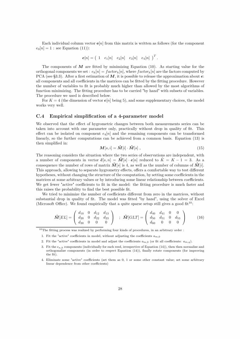
We tried to minimize the number of coefficients different from zero in the matrices, withoutsubstantial drop in quality of fit. The model was fitted "by hand", using the solver of Excel(Microsoft Office). We found empirically that a quite sparse setup still gives a good fit10:

M [EL] =

d10 0 d12 d13

d20 0 d22 d23

d30 0 0 0

; M [GLT ] =

d40 d41 0 0d50 d51 0 d53

d60 0 0 0

(16)

10The fitting process was realized by performing four kinds of procedures, in an arbitrary order :

1. Fit the "active" coefficients in model, without adjusting the coefficients am,0

2. Fit the "active" coefficients in model and adjust the coefficients am,0 (or fit all coefficients: am,q).

3. Fit the en,k components (individually for each reed, irrespective of Equation (14)), then then normalize andorthogonalize components (in order to respect Equation (14)), finally rotate components (for improvingthe fit).

4. Eliminate some "active" coefficients (set them as 0, 1 or some other constant value; set some arbitrarylinear dependence from other coefficients)

28

M [SeriesA] =

1 0 0 0 00 1 0 0 00 0 1 0 00 0 0 1 0

; M [SeriesB] =

1 0 0 0 0c10 1 0 0 0c20 0 c22 0 c24

c30 0 0 1 0

(17)

This corresponds to the hypothesis named H5. Furthermore some coefficients may be propor-tional to others, without noticeable drop in quality of fit. This diminishes the number of "active"coefficients in the different matrices from 18 to 9 (hypothesis H4):

d22 = 2d12 ; d13 = d12 = − d23;

d40 = d50 = 6d41 ; d51 = 2d41 = −d53 ; (18)

c22 = c24 = 1/2.

C.5 Adjusting coefficients for removing systematic errors

After fitting the different models, we observed some systematic deviations in the resonancefrequencies between model and observations. This error has probably two different origins:an inevitable inaccuracy in the FEM computation (and in our metamodel) and an error forparameters not included in the model. A straightforward way to minimize the residuals is toadjust the coefficients am,0 in Equation (1)11. Fitting all coefficients in Equation (1) is doubtlessa more questionable way to reduce this error (hypotheses H8 and H9). This can reduce the meandeviation between model and observations, but greatly increases the number of coefficients inthe model (see however the discussion §4.4).

C.6 Testing different hypotheses

We tested different hypotheses with our model, in order to select a particularly efficient model.Some of them are summarized in the Table 11.

Hypotheses H1 to H3 (elastic model) present a poor fit; the adjustments for coefficients am,0

are large, compensating partially the missing viscoelastic components. All viscoelastic modelsare notably better and exhibit smaller adjustments for am,0. Frequency dependence for EL andGLT seems evident. Hypothesis H4 shows a good accuracy, with only 9 fitted coefficients (and 11adjustments). Augmenting the number of coefficients up to 60 brings only a marginal contribution(H5 to H7). Adjusting the other coefficients of Equation (1) in H8 and H9 improve the model,especially for the high modes. Our FEM computations (and consequently our metamodel) areprobably attached with systematic errors in this frequency range. The influence of ET shouldeventually be considered. Between H8 and H9, the total number of components (N ×K) increasesfrom 220 to 660. The adjustments within morphological classes are related: “flexural” modesshows systematically lower values than neighboring “transversal” modes.

C.6.1 Backward random validation

Following a suggestion by a referee, we applied a principal component analysis to simulated datacomputed after hypothesis H5: we assigned randomly a value for the 4 components and 55 reeds,following a normal distribution. We repeated this operation ten times. As expected, the PCAdetected 4 factors capturing 91.2% (Standard Deviation 1.3%) of the variance of the simulated

11These coefficients can be fitted through the fitting procedure (some constraints have however to be introduced,to avoid an important deviation from their theoretical values) or merely adjusted, so that the total averageddeviation for each mode and both series is 0.

29

Hypothesis K model #ActiveCoef #OtherCoef RMSD

H1 0 elastic 2 am,0 → 11 76.2H2 2 elastic 4 am,0 → 11 54.8H3 3 elastic 7 am,0 → 11 43.9H4 4 viscoelastic 9 am,0 → 11 30.4H5 4 viscoelastic 18 am,0 → 11 29.8H6 4 viscoelastic 44 am,0 → 11 29.1H7 4 viscoelastic 60 am,0 → 11 28.6H8 4 viscoelastic 60 am,q → 66 23.2H9 12 viscoelastic - am,q → 66 19.8H10 4 regression - Ws,m,k → 110 21.8

H11 4 regression 4 Wm,k → 44 24.7

Table 11: Synthesis of some hypotheses tested with our model. K: Number of componentsfor each reed n; model: elastic, viscoelastic or multiple regression (with the elastic model, EL

and GLT are independent from frequency; the elastic model is computed after the viscoelasticone by setting very small values for the coefficients affecting E2, E3, G2 and G3, in order toavoid division by 0; multiple regression: see Equations (19 and 20)); #ActiveCoef : number

of "active" coefficients in the matrices M or M and M (fitted through the fitting procedure);#OtherCoef : number of other coefficients estimated in model (am,0: adjusted so that themean error for each mode m and both series is zero, Ws,m,k: computed analytically, otherwise:fitted through the fitting procedure); RMSD [in cents] after Equation (10): this is a measure ofgoodness of fit (remember that the vibration patterns of the reeds were observed in steps by 25cents). The results are commented in the text.

data (mean: 42.6, 20.9, 16.2 and 11.5% for each factor). This seems compatible with the analysisperformed on the observed frequencies (§ 3.3): 4 factors: 91.2% of the variance (53.6, 21.4, 10.8and 5.4% for each factor).

D Reconstructing observed resonance frequencies by mul-

tiple regression

The scheme of our viscoelastic model is:〈vector e〉 → {multiple regression Equation (13)} → 〈viscoelastic coefficients v〉 → {viscoelasticmodel Equation (4)} → 〈moduli E′

L and G′

LT 〉 → {metamodel Equation (1)} → 〈reconstructedresonance frequencies r〉.

It has a very interesting property: the same model of cane can be used for any kind of reeds(for instance bass clarinet or saxophone) or for any other boundary conditions. Only Equation(1) has to be changed (or at least, the coefficients am,q have to be recomputed).

Within our particular setup, the viscoelastic model is however not required for reconstructingthe observed resonance frequencies: PCA is theoretically the optimal linear scheme, in terms ofleast mean square error, for compressing a set of high dimensional vectors into a set of lower di-mensional vectors and then reconstructing the original set by multiple regression. The shortenedscheme is merely:〈vector factor〉 → {multiple regression} → 〈reconstructed resonance frequencies r〉.

Let us examine this option. For this purpose we use the array factorn,k computed in § 3.3,holding our 4 principal components (factors). As before (§C.3), we set factorn,0 = 1. The array

30

of reconstructed resonance frequencies rn,s,m can be computed by multiple regression using anarray of matrices Ws,m,k:

r[n, s] = W [s] · factor[n] (19)

As before (§C.4), we have also the option to reduce the dimensionality from K to K, using the

previously defined array of matrices M [s] and then use a unique matrix Wm,k to operate themultiple regression:

r[n, s] = W · M [s] · factor[n] (20)

We call these 2 options: hypotheses H10 and H11. For H11, we performed a small orthogonalrotation of the factors to concentrate the information about the hygrometric material propertiesin factorn,4, for a better fit. The results are summarized in Table 11.

Multiple regression is an accurate way to retrieve our measurements, comparable to H8 andH9. With only 48 coefficients, H11 is very efficient, even better for “transversal modes” as H10.The results of the regressive model are more difficult to interpret as those of the viscoelasticmodel. As en,4 before, factorn,4 serves uniquely to adjust factorn,2 relatively to series B. Asexpected, factorn,1 influences mainly the “transversal modes” and factorn,2 the “flexural modes”.

Their respective coefficients in the matrix W reflect this antinomy. “Transversal” and “flexuralmodes” are concerned by factorn,3 in a quite similar way, but the slope is not same.

References

[1] H.C. Spatz, H. Beismann, F. Brüchert, A. Emanns, and T. Speck. Biomechanics of the giantreed Arundo donax. Philosophical Transactions of the Royal Society of London. Series B:Biological Sciences, 352(1349):1, 1997.

[2] E. Marandas, V. Gibiat, C. Besnainou, and N. Grand. Caractérisation mécanique des anchessimples d’instruments à vent. J. Phys. IV France, 4:C5–633, 1994.

[3] S. Ollivier. Contribution à l’étude des oscillations des instruments à vent à anche simple:Validation d’un modèle élémentaire. PhD thesis, Université du Maine, Le Mans, France.,2002.

[4] J.P. Dalmont, J. Gilbert, and S. Ollivier. Nonlinear characteristics of single-reed instru-ments: Quasistatic volume flow and reed opening measurements. The Journal of the Acous-tical Society of America, 114:2253, 2003.

[5] O. Speck and HC Spatz. Mechanical Properties of the Rhizome of Arundo donax L. Plantbiol (Stuttg), 5:661–669, 2003.

[6] O. Speck and H.C. Spatz. Damped oscillations of the giant reed Arundo donax (Poaceae).American journal of botany, 91(6):789, 2004.

[7] Ph. Chevaux. Améliorations de la durée de vie des anches doubles en roseau pour instrumentsà vents. Projet de fin d’étude, Institut National des Sciences appliquées de Lyon, France,1997.

[8] E. Obataya. Physical properties of cane used for clarinet reed. Wood Res. Tech. Notes,32:30–65, 1996.

[9] E. Obataya, T. Umezawa, F. Nakatsubo, and M. Norimoto. The effects of water solubleextractives on the acoustic properties of reed (Arundo donax L.). Holzforschung, 53(1):63–67, 1999.

31

[10] E. Obataya and M. Norimoto. Mechanical relaxation processes due to sugars in cane (Arundodonax L.). Journal of Wood Science, 45(5):378–383, 1999.

[11] E. Obataya and M. Norimoto. Acoustic properties of a reed (Arundo donax L.) used for thevibrating plate of a clarinet. The Journal of the Acoustical Society of America, 106:1106–1110, 1999.

[12] A.E. Lord. Viscoelasticity of the giant reed material Arundo donax. Wood Science andTechnology, 37(3):177–188, 2003.

[13] D. Casadonte. The perfect clarinet reed? Vibrational modes of realistic clarinet reeds. TheJournal of the Acoustical Society of America, 94:1807, 1993.

[14] D. Casadonte. The clarinet reed: an introduction to its biology, chemistry and physics. PhDthesis, Ohio State University, 1995.

[15] M. Facchinetti, X. Boutillon, and A. Constantinescu. Application of modal analysis and syn-thesis of reed and pipe to numerical simulations of a clarinet. The Journal of the AcousticalSociety of America, 108:2590, 2000.

[16] M.L. Facchinetti, X. Boutillon, and A. Constantinescu. Numerical and experimental modalanalysis of the reed and pipe of a clarinet. The Journal of the Acoustical Society of America,113:2874, 2003.

[17] T. Guimezanes. Etude Expérimentale et Numérique de l’Anche de Clarinette. PhD thesis,Université du Maine, Le Mans, France, 2007.

[18] F. Pinard, B. Laine, and H. Vach. Musical quality assessment of clarinet reeds using opticalholography. The Journal of the Acoustical Society of America, 113:1736, 2003.

[19] P. Picart, J. Leval, F. Piquet, J.P. Boileau, T. Guimezanes, and J.P. Dalmont. Tracking highamplitude auto-oscillations with digital Fresnel holograms. Optics Express, 15(13):8263–8274, 2007.

[20] P. Picart, J. Leval, F. Piquet, JP Boileau, T. Guimezanes, and JP Dalmont. Study of theMechanical Behaviour of a Clarinet Reed Under Forced and Auto-oscillations With DigitalFresnel Holography. Strain, 46(1):89–100, 2010.

[21] D. Mounier, P. Picart, J. Leval, F. Piquet, J.P. Boileau, T. Guimezanes, and J.P. Dalmont.Investigation of clarinet reed auto-oscillations with digital Fresnel holography. The Journalof the Acoustical Society of America, 123:3240, 2008.

[22] IT Jolliffe. Principal component analysis. Springer verlag, 2002.

[23] U. Schnars and W. Jüptner. Direct recording of holograms by a CCD target and numericalreconstruction. Applied Optics, 33(2):179–181, 1994.

[24] F. Joud, F. Laloë, M. Atlan, J. Hare, and M. Gross. Imaging a vibrating object by SidebandDigital Holography. Optics express, 17(4):2774–2779, 2009.

[25] F. Joud, F. Verpillat, F. Laloë, M. Atlan, J. Hare, and M. Gross. Fringe-free holographicmeasurements of large-amplitude vibrations. Optics Letters, 34(23):3698–3700, 2009.

[26] Claripatch SA website. http://www.claripatch.com.

32

[27] Wikipedia. http://en.wikipedia.org/wiki/Principal_component_analysis.

[28] Systat. http://www.systat.com.

[29] D. Roylance. Engineering viscoelasticity in 3.11 OpenCourseWare . Departament of Mate-rials Science and Engineering Massachusetts Institute of Technology, Cambridge, 2001.

[30] A. Chaigne, J. Kergomard, and X. Boutillon. Acoustique des instruments de musique. Belin,2008.

[31] E.H. Dill. Continuum mechanics: elasticity, plasticity, viscoelasticity. CRC, 2006.

[32] L. Gaul and A. Schmidt. Experimental Determination and Modeling of Material Damping.VDI-Berichte; Schwingungsdämpfung, 2003:17–40, 2007.

[33] J. M. Heinrich. Recherches sur les propriétés densitométriques du matériau cane de Provenceet ses similaires étrangers; relation avec la qualité musicale; étude associée d’une mesure dedureté. Technical report, Ministère de la Culture, Direction de la Musique et de la Danse,France, 1991.

[34] A. Saltelli, M. Ratto, T. Andres, F. Campolongo, J. Cariboni, and D.S. Gatelli. GlobalSensitivity Analysis. The Primer. John Wiley & Sons Chichester, England.

33