Measurements of Free Form Surfaces and Best-fitting ...

Measurements of Free Form Surfaces and Best-fitting

Measurements of Free Form Surfaces and Best-fitting

Mexican CMM Club MeetingVOLKSWAGEN de México (VWM)

Puebla, Pue., México22 October 2007

Mexican CMM Club MeetingVOLKSWAGEN de México (VWM)

Puebla, Pue., México22 October 2007

Kostadin DoytchinovInstitute for National Measurement Standards National Research Council [email protected]

Kostadin DoytchinovInstitute for National Measurement Standards National Research Council [email protected]

Kotem Technologies Inc.www.kotem.com

Free Form Surface

The skin of a 3D geometric element which do not have rigid radial dimensions, unlike regular surfaces such as planes, cylinders

and conical surfaces.

Examples: turbine blades, gear surfaces, car bodies, aircraft

bodies, etc.

Free Form Area

Free Form Surface

Examples: turbine blades, gear surfaces, car bodies, aircraft bodies, etc.

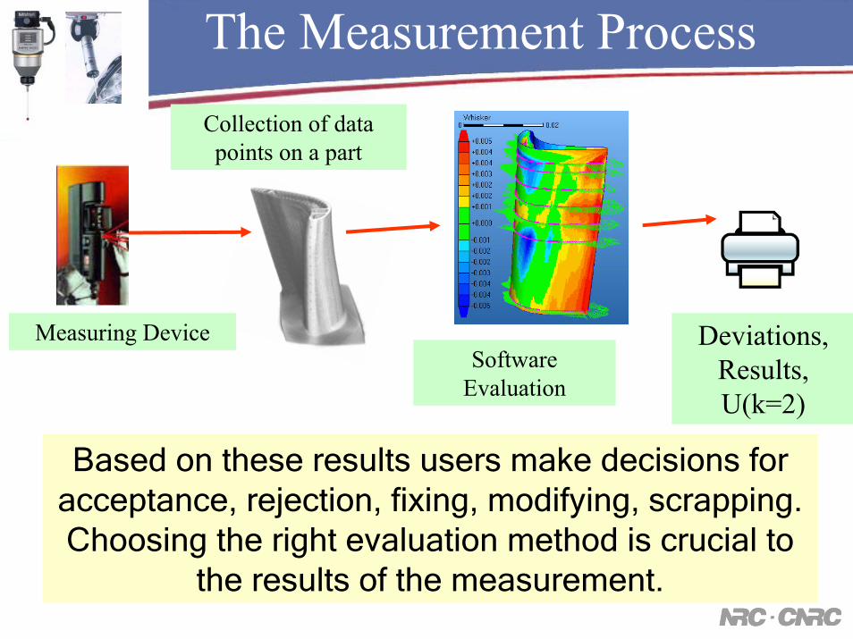
The Measurement ProcessCollection of data points on a part

Software Evaluation

Measuring Device Deviations, Results, U(k=2)

Based on these results users make decisions for acceptance, rejection, fixing, modifying, scrapping. Choosing the right evaluation method is crucial to

the results of the measurement.

The Measuring Instruments

Principles of Sensors of Modern CoordinateMeasuring Systems:

• tactile switching 3D• tactile analog 3D• optical 2D camera• optical video auto

focus• optical triangulation

– laser scanners– photogrametry

• optical point focus

• tactile-optical• optical

interferometric– laser trackers

• optical time of flight• X-ray• GPS, radar, etc.

Cartesian CMMs

Articulating Arm Systems

ROMER

FARO

CMMs (Non-Cartesian) – Laser Trackers

Major suppliers: Leica, Faro, API

Uncertainties of measurement starting at about 10 µm and up. The shape of the uncertainty zone is dominated by the lower uncertainties of the two angles.

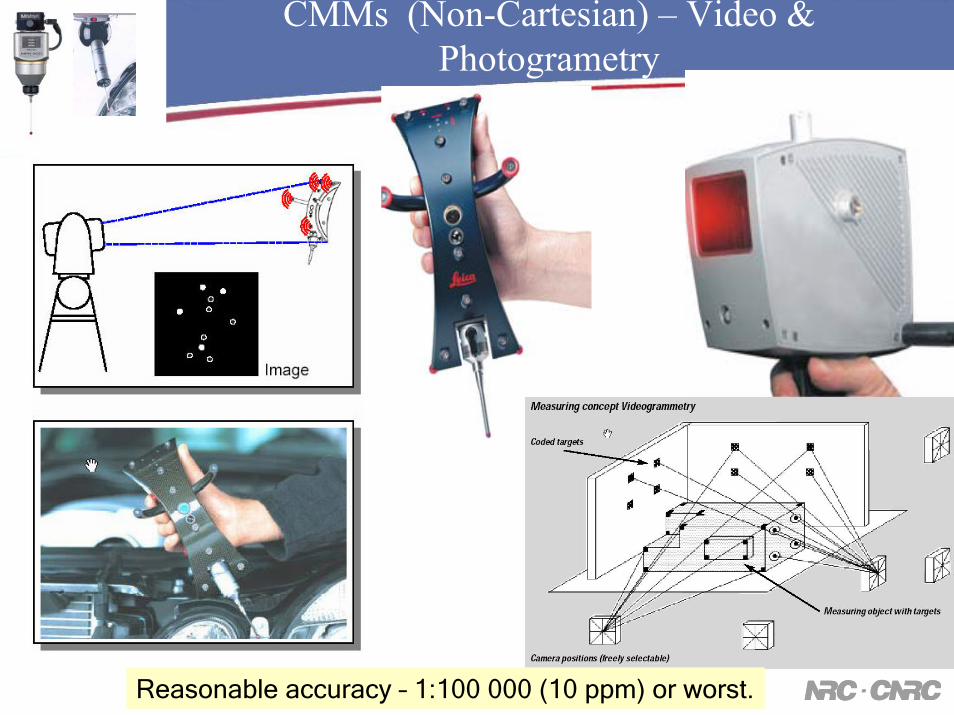
CMMs (Non-Cartesian) – Video & Photogrametry

Reasonable accuracy – 1:100 000 (10 ppm) or worst.

OGP

Mitutoyo

OGP

Traditional Video Measuring Machines

Scanner conceptAdvantages: high data density, high speed - tenths of 1,000s of points/sec

Disadvantages: relatively low accuracy, sensitive to surface finish

Scanner on a CMM

Laser Scanners

Applications: reverse engineering, sheet metal parts, free form surfaces

Metris

Fringe Projection Systems

camerasprojector / scanner

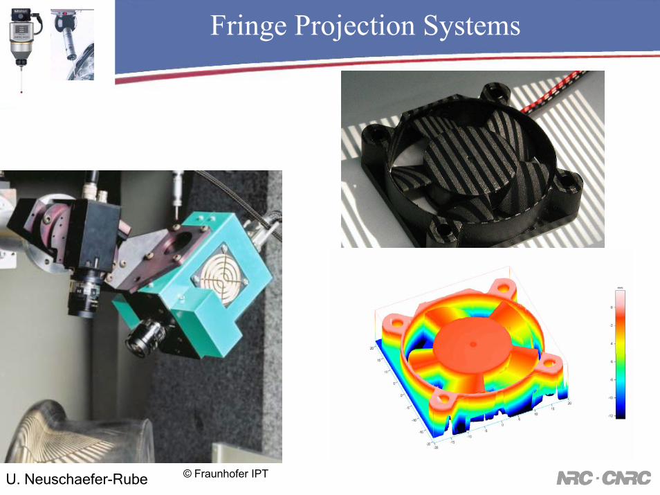
Fringe Projection Systems

© Fraunhofer IPTU. Neuschaefer-Rube

Sheet Metal Examples

Benteler Automotive

Benteler Laser Gauge

The optical methods are replacing traditional CMMs for data collection when tolerances

allow. Uncertainties range typically 30-100 µm with

measurement time down to 1-2 minutes and huge data density –

millions of points.

Systems with a Tip (Stylus)

Physical Tip with a known radius

Surface Measurements – Data Collection

– Free form surfaces require much higher point density for proper surface evaluation

– Parts with free form surfaces tend to have larger tolerances attached

– The above facts favor the optical methods• High data density• Uncertainties still kept in workable proportion

to the tolerance zones – 1:10, 1:5

Surface Measurements – Data Collection

– The data high density – millions of points is not always an advantage

• The number of point overwhelms the computer capabilities and slows down the evaluation process.

• Data very often needs filtering to improve accuracy and reduce data noise.

– The evaluation process requires different software capabilities

The Goal of the Measurement Determines the Evaluation Process

Tolerance Compliance

Manufacturing Process Analysis

SPC (Statistical Process Control)

Data Evaluation Process

Data Collection (Measurement)

Need for task specific evaluation: the analysis may lead to very different results using the

same raw data!

Surface Measurements

• Measurements of an unknown geometry –nominal information– Reverse engineering

• Measurements of a known geometry – we have a drawing or a CAD model– Control for compliance– Troubleshooting

If the real geometry deviates significantly from the theoretical one, at one point, depending on the accuracy required it

should be treated as “unknown”.

Tip Radius Compensation on a Free Form Surface

The effective tip radius should be corrected from the tip center, to the surface in the direction of the estimated normal vector at the point of contact. Poor estimation of the normal vector leads to cosine errors.

Tip radius correction - cosine error

Error R a= × −( cos( ))1

The cosine error is proportional to thetip radius and to the cosine of the angle between the real and estimated spatial normal vectors

Tip Radius Correction - Cosine Error

Normal vector error in degrees

2.5 5 10 301 1.0 4 15 134

1.5 1.4 6 23 201

2 1.9 8 30 268

9.75 9.3 37 148 1306

Tip

radi

us R

(mm

)

Cosine error (µm)Laser tracker typical tip

radius

Tip Radius Correction for Geometrical Features

For machined parts with regular surfaces the cosine errors are

usually negligible

Attention has to be paid when measuring parts with large curvatures and castings

Surface Measurements – Known Geometry – Tip Radius Compensation

• CAD model available – tip radius is compensated perpendicular to the surface

– Results depend on the part alignment (best-fit).

Center of tip points Tip Radius compensated points

Measurements of a known geometry

Example: 10.256, 36.975, -15.218, 0.45678, 0.56124, 0.69019

Data from given as: X, Y, Z, i, j, k

X

Y

The data should be given in a well defined coordinate system (set-up) – otherwise not reliable. Typically, it requires datum target definition. The CMM is then programmed to measure the points in a direction opposite to the normal vector (pointing out of the material).

( )i j k2 2 2 1+ + =

ConditionDiscrete point information

Vectoring Accuracy

∆ = − + − + −( ) ( ) ( )NX X NY Y NZ Z2 2 2True position(reported from the CMM)

NX, NY, NZ

X, Y, Z

The “true position” contains theCMM “vectoring” errors (the inabilityof the CMM to drive the probe indefined direction). This can be a majorproblem since many of the CMMs donot have a good “ vectoring” accuracy.

Actual CMM trajectory

Vectoring accuracy

Approach vector

The component of the “true position”which is caused by the “vectoring errors’can be significant if higher accuracy isrequired. If the tip radius is compensated after best-fitting, these errors can be greatly reduced.

Vectoring Accuracy

0, 0, 0

Simple experiment for vectoring error estimation. Can be repeated in several orientations

Our SIP 560M CMM had vectoring errors up to 40 µm

Our Legex CMM has vectoring errors below to 0.2 µm

Surface Measurements – Known Geometry – Tip Radius Compensation

• CAD model available – tip radius is compensated perpendicular to the surface

– Results depend on the part alignment (best-fit).

Center of tip points Tip Radius compensated points

Tip Radius Compensation

X= 198.355

Y= -18.168

Z= 236.677

Tip center coordinates

Uncertainty zone

Plus the knowledge that this point is one tip radius away from the real surface if a tip

radius is present

Compensating the tip radius during the best-fitting is the right approach, but in certain conditions this may not be accurate enough.

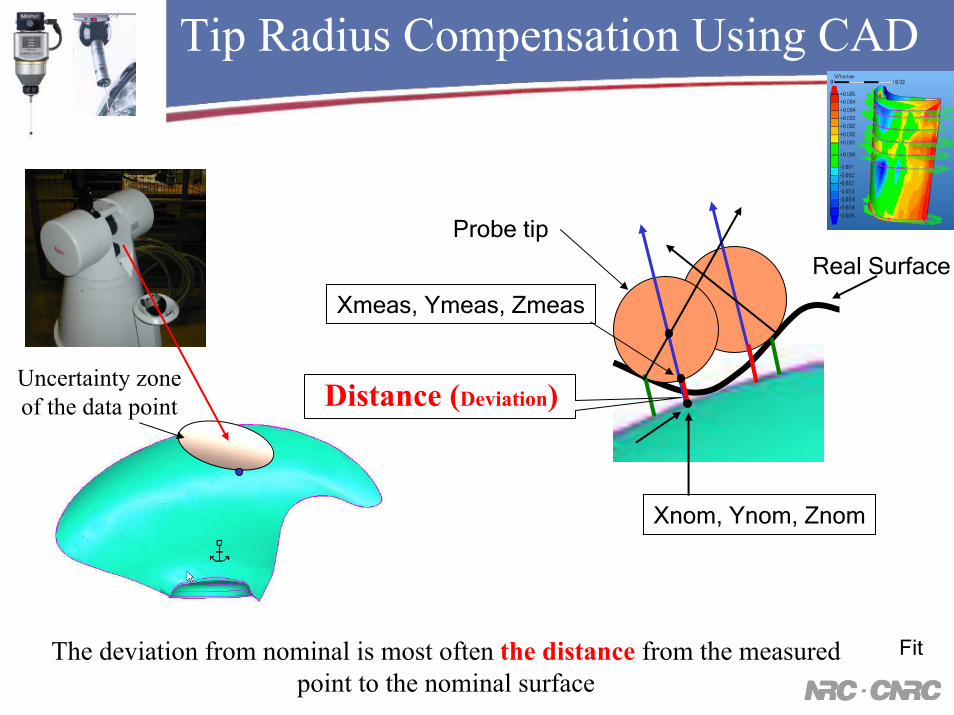
Tip Radius Compensation Using CAD

Distance (Deviation)Uncertainty zone of the data point

Xmeas, Ymeas, Zmeas

Real Surface

Probe tip

Xnom, Ynom, Znom

The deviation from nominal is most often the distance from the measured point to the nominal surface

Fit

Uncertainty due to Tip Radius Compensation

In this case the rotation was 0.2 degrees which will move a point 1.5 metres from origin by 5 mm

from the original position.

Courtesy of Kotem

5 mm on an area with high curvature may mean a very

different normal vector applied to the same point!

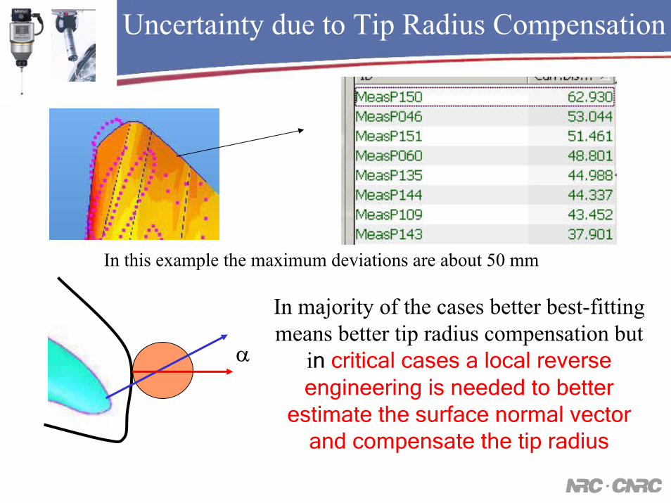
Uncertainty due to Tip Radius Compensation

In this example the maximum deviations are about 50 mm

α

In majority of the cases better best-fitting means better tip radius compensation but

in critical cases a local reverse engineering is needed to better

estimate the surface normal vector and compensate the tip radius

The Nominal Data

CAD Geometry Problems

Reversed surface normal vectors

Seeing surfaces with bright and dark colors when opening a file should be investigated

Reported deviations will be with opposite sign and the results wrong

Inaccurate CAD Geometry

Check the CAD geometry before best-fittingLow Accuracy Model

This nominal cylinder has a form error of 0.012 mm built in!

Fitting measured points to this surface will be affected

CAD to CMM Data FlowGeometry Description – Model Accuracy

The center position of this “nominal cylinder” is

questionable!

CAD to CMM Data FlowExamples of Problems

Propeller CAD model

This model visibly looks fine. Only after thorough examination one can discover problems which could cause uncertainty

On one of the blades, some small surfaces have a normal vectors pointing inside the material! During measurements this may cause some deviation to change sign.,

With a very high magnification it is visible that part of the surface is missing and we can see through the gap inside the blade!

CAD to CMM Data Flow

IGES

STEPCAD systemnative format

PlanesCylindersCircles, X.Y.Z,i,j,k……….

CMM software

Programexecution

CMM

During the conversion from native CAD format to IGES, VDA or STEP, some of the geometrical data may be modified or lost! The result is that the CMM is working with a model different from the original! The model may end up incomplete and with many faults in it.

?

The CAD systems very rarely use generic equations when describing simple elements as cylinder, cone, circle. They may all be described with NURBS (splines)! At the same time the user expects, for example, a radius and a hole center location. This forces the CMM software to “calculate” the nominal dimensions of elements from spline surfaces. This a source of additional uncertainty.

NURBS,Elements,………?

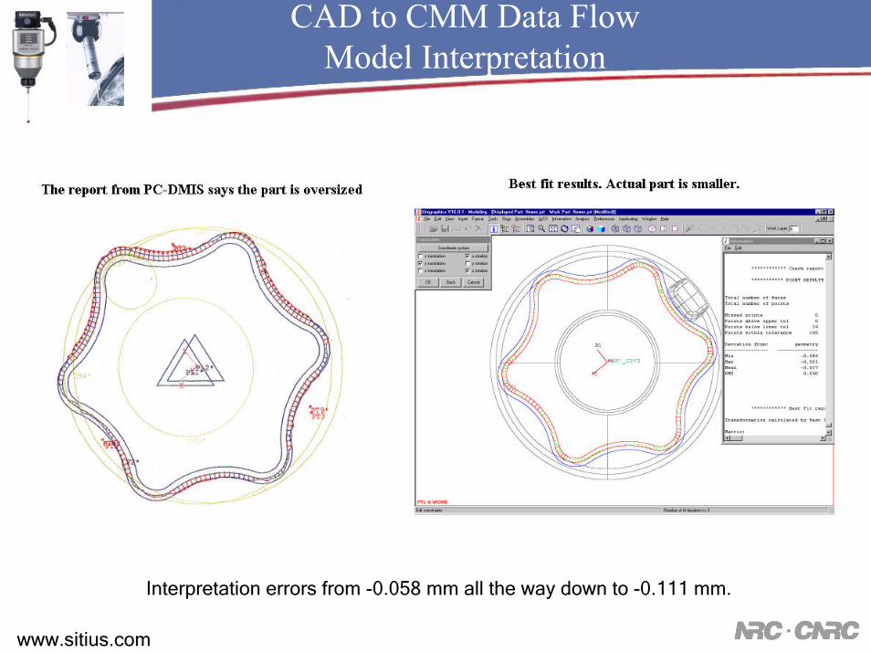
CAD to CMM Data FlowModel Interpretation

Interpretation errors from -0.058 mm all the way down to -0.111 mm.

www.sitius.com

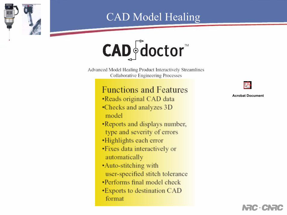
CAD Model Healing

Acrobat Document

CAD to CMM Data FlowExamples of Problems

To address the issue, numerous CAD model “healing packages exist”. It is important to note that some problems are reparable just fine, while others require modifications of the model. The client has no idea how the “healing” is done. The only thing he notices is that the file does not crash anymore… These modifications are a source of uncertainty.

Practical way of assessing the accuracy of the data transfer

IGESSTEP

CAD systemnative format

The CMM software generates points with X,Y,Z,i,j,k on the critical surfaces of the model or on the whole model

CMM software

0. ≈MaxDistGoal:The so created points are imported back into the original CAD system and a calculation is performed for the distance between the points and the original model. If the transfer is good, the distances should be negligible.

What is Best-fitting ?

Best-fitting is the process of finding the best mutual relationship between Measured data and Nominal data when the part is not fully constrained while

trying to satisfy a specific goal.

X

Y

X

Y

Sheet Metal

Datum Points

Best-fitting

After Best-fitBefore Best-fit

Constrained Features – Soft GaugesSoftware gauge

Hard gaugeDrawingConstrained cylinders

Complete assessmentNon-constrained cylinders

Complete assessment

Weckerman, Heinrichowski and Mordhorst,

Best-fitting of Shapes and Patterns

• We best-fit for the purpose of:– Comparison

• Measured data to nominal (Example: to satisfy tolerances)• One part to another part

– Assembly• To show that parts fit well in an assembly• To analyze an assembly

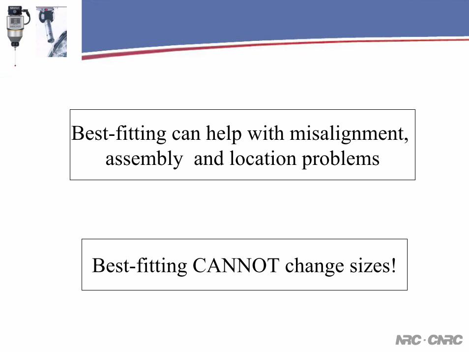
Best-fitting can help with misalignment, assembly and location problems

Best-fitting CANNOT change sizes!

Measuring Device - Software Integration

X, Y, Z measured coordinates plus tip radius when applicable

Best-fit and Analysis Software

CAD Model – IGES, VDA,DXF, STL

The Best-fitting Environment

Nominals/CAD

Measured Data

Math Criteria

Weights/Exclude

Tolerances

Releases

FiltersCalculations

Groups

Statistics

Result 2Result 1 Result N

Best-fitting Process

Transferring the Result

Locator # RemarksLOC1

LOCATOR AN 1 /LOCA# 1Z = 0.000 Z = -0.223

LOC2 LOCATOR AN 2 /LOCA# 20 000 0 9Z = 0.000 Z = -0.043

LOC4 LOCATOR AM 1 /LOCA# 4Y = -0.200 Y = -0.435

LOC5 LOCATOR AM 2 /LOCA# 5Y = 24.880 Y = 24.669

LOC6 LOCATOR C /LOCA# 6X = -0.367 X = -0.559

LocatorsCurrent coordinatesOriginal coordinates

ORRPS – Reference Point System

Best-fitting Principles

Point-to-point Points-to-surface

The measured points are not associated to a particular point. During the procedure with every iteration a new “iterative closest point” is calculated.

There is an association of measured point to a nominal point

MEAS (X,Y,Z) NOM (X,Y,Z)

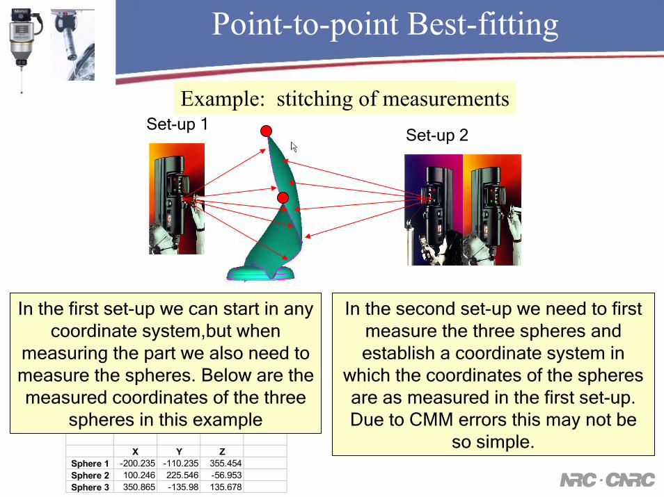
Point-to-point Best-fitting

3D Case – Using Spheres

Set-up 1Set-up 2

Example: stitching of measurements

X Y ZSphere 1 -200.235 -110.235 355.454Sphere 2 100.246 225.546 -56.953Sphere 3 350.865 -135.98 135.678

In the first set-up we can start in any coordinate system,but when

measuring the part we also need to measure the spheres. Below are the measured coordinates of the three

spheres in this example

In the second set-up we need to first measure the three spheres and establish a coordinate system in

which the coordinates of the spheres are as measured in the first set-up. Due to CMM errors this may not be

so simple.

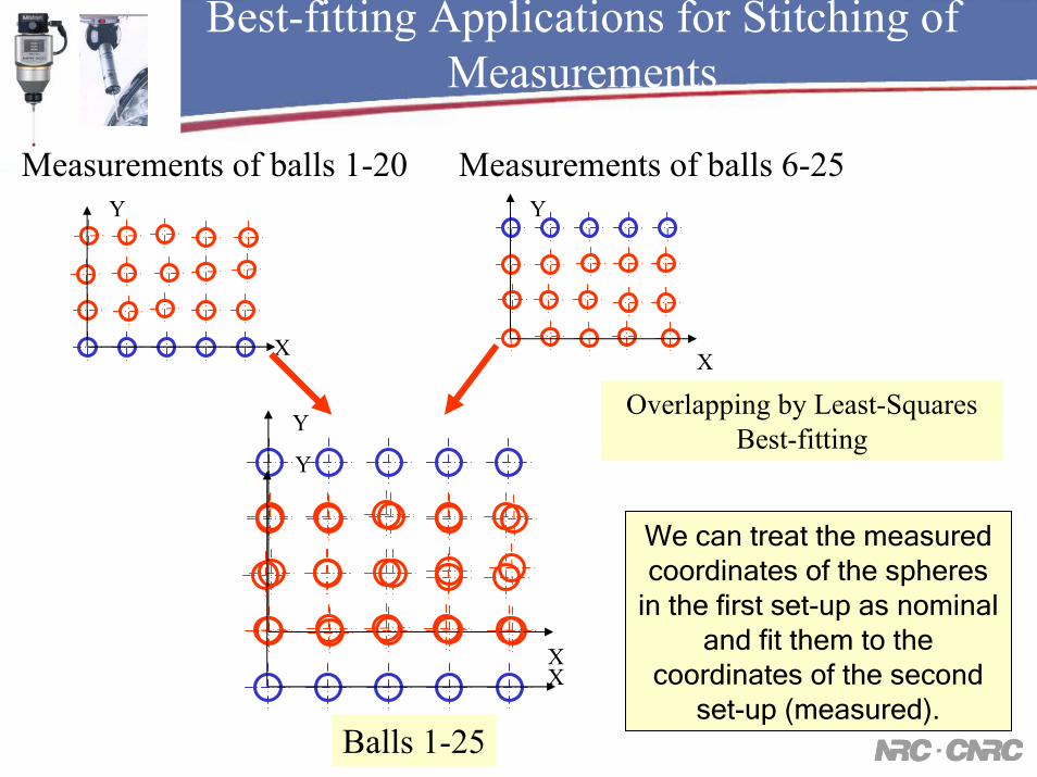
Best-fitting Applications for Stitching of Measurements

Measurements of balls 1-20 Measurements of balls 6-25

X

Y

X

Y

X

Y

X

Y

Overlapping by Least-SquaresBest-fitting

We can treat the measured coordinates of the spheres

in the first set-up as nominal and fit them to the

coordinates of the second set-up (measured).

Balls 1-25

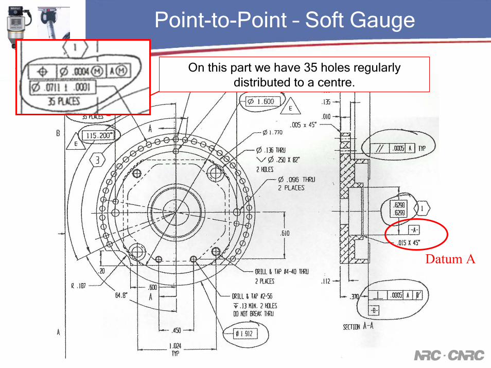
Point-to-Point – Soft Gauge

On this part we have 35 holes regularly distributed to a centre.

Datum A

Point-to-point Best-fitting

Example: Measured hole center locations are fitted to the nominal center locations described by the drawing (CAD)

Point-to-surfaces Best-fitting

Example: Measured individual points are fitted to the nominal surfaceCAD geometry without a circle calculation - typical profile tolerancing

Conditions for Best-fitting

– No Datum Reference Frame at all.– Datum Reference Frame does not fully

constrain a coordinate system. – Mobility of datums specified at MMR or

LMR - boundary constrained best-fit.– Datum Reference Frame uses multiple

features for single datums– “What if” analysis.


No Datum Reference Frame at all

0.2


Datums do not fully constrain a coordinate system.

Floating profile – no real datum in the plane

Means this

If evaluated without “best-fitting” the bias in the results by half of the tolerance zone is almost guaranteed!


Datums do not fully constrain the coordinate system.

Datums K and M together can constrain 5 degrees of freedom. The rotation about the Z axis is unconstrained.

Z


Example: Composite Positional Tolerancing

Feature-Relating Tolerance Zone Framework (FRTZF)

Tolerance Zones

Pattern-Locating Tolerance Zone Framework (PLTZF)

One Symbol for Position

Reproduced from ASME Y14.5M-1994

8.0φ 25.0φ

Best-Fitting Tools Influencing the Results

• Mathematical Criterion• Weight factor conditions• Tolerancing conditions

– Mix of toleranced and non-toleranced features.• Degrees of freedom and Constraints

– Constraint of rotations (about X,Y,Z)– Constraint of translations (X,Y,Z)– Constraint about a specific point in space

• Starting point for the optimization– Ability to avoid local minimums

• Possibility to make repeated optimization runs• Additional Tools

– Filters– Assembly simulations

The Mathematical Criteria

Mathematical Criteria

The best-fitting criterion is the mathematical approximation of the practical goal we are trying to achieve

• Examples of possible goals:– Determine the best fit from averaging point of view– Verify if a part satisfies a tolerance

• Satisfy a tolerance zone and at the same time other requirements

– Verify that parts can fit into an assembly– Determine if a part can be machined from a casting– Influence results to save time/money/other goals


The best-fitting criterion is the mathematical approximation of the practical goal we are trying to achieve

• Examples of criteria:– Least Squares– Sum of the absolute values of deviations– Min-Max– Uniform deviations– Tolerance envelope– Tolerance envelope Min-Max– Etc.

Mathematical Criteria)( 2∑∆= iMinFi∆

• The most commonly used criterion• Very stable• Best averaging effect• Not sensitive to the sign of the deviations

– Should not be used where sign is important• The result is not influenced by the prescribed tolerance

– NOT to be used when tolerances present unless no other possibilities!

Least Squares Criterion (LS)

Nominal Surface


Out∆

The Tolerance Envelope Criterion

• The goal of this criterion is to bring the measured points in tolerance

• Does not optimize the in-tolerance distribution– Only works with the points out of tolerance– Separate criterion needed to improve inside the tol.zone

• Affected by outliers

)( 2∑∆= OutMinF

The Min-Max Criterion

• The goal of this criterion is to reduce the maximum deviation to the minimum possible

• Directly minimizes the maximum profile deviation• Almost equivalent to the Tolerance Envelope with uniform

tolerance zone• Affected by outliers

MINMAX =∆

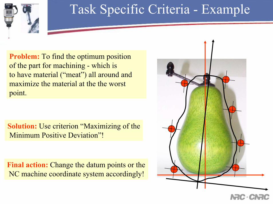
Task Specific Criteria - Example

Problem: To find the optimum positionof the part for machining - which isto have material (“meat”) all around andmaximize the material at the the worst point.

Solution: Use criterion “Maximizing of theMinimum Positive Deviation”!

Final action: Change the datum points or theNC machine coordinate system accordingly!

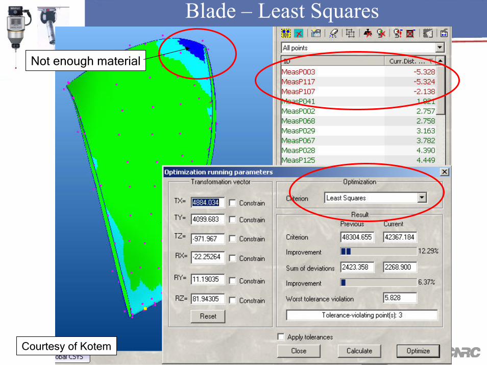
Blade – Least Squares

Not enough material

Courtesy of Kotem

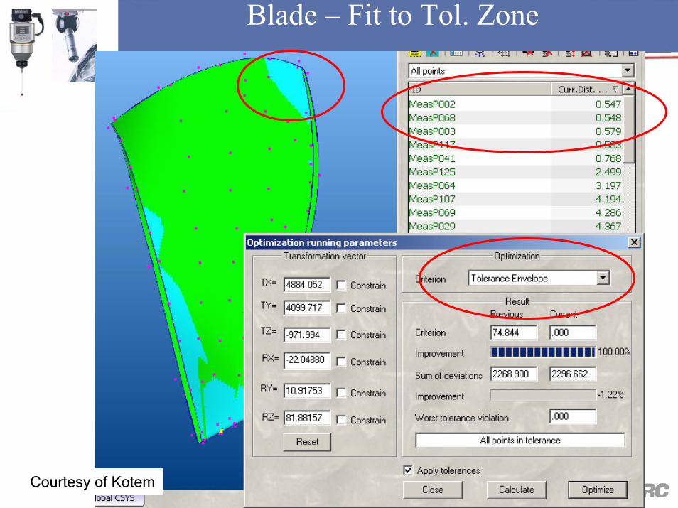
Blade – Fit to Tol. Zone

Courtesy of Kotem

Courtesy of Kotem

Blade – Special Criterion

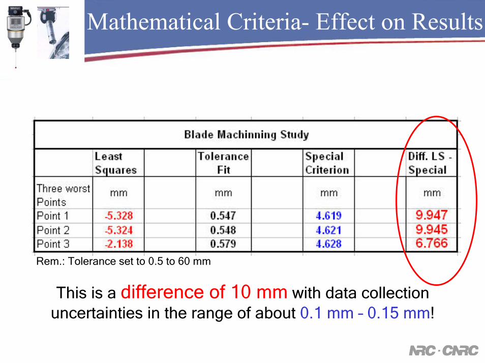
Mathematical Criteria- Effect on Results

This is a difference of 10 mm with data collection uncertainties in the range of about 0.1 mm – 0.15 mm!

Rem.: Tolerance set to 0.5 to 60 mm


There isn’t a always a “perfect criterion”and starting conditions which does the job.

The time and money requirements define the “right” criterion and starting conditions!

The best-fitting gives a choice to the engineer to save money and time!

It teaches an attitude towards the process –always try to extract the best!

Tools - Using Weight Factors

Original Result

Weighted Result with w=10

Using weight factors is a very important tool helping to find the right compromise and save money and time


• We can move errors to areas of the part where we can re-work them easily

• Avoid or reduce welding required to re-work tooling

• The goal is not to bring a feature to a zero deviation! It is to move it to where the overall solution is more acceptable.

Using weight factors is a very important tool helping to find the right compromise and save money and time


Original Result

Weighted Result with w = 0

Using weight factor = 0 is a very important tool in eliminating outliers and determining their correct

positions after optimization


Example: P1 and P2 are both of tolerance after best-fit. This would mean both need to be fixed

Tolerance

P1 P2

Dev Dev

After excluding P2 there is only one point to be fixed

P1 P2 (W-0)

Dev

Point-to-Point – Tolerance Envelope

Mobility Zone of Datum A

Although this is 3D case, taking into account the specifics it is better to approach it as a 2D case

Due to MMC the tolerance zone of the hole centers can be different depending on the size

Datum Targets

Datum Target Point

Datum Target Area

• This is the typical 3-2-1 concept

• Three points for a plane

• Two points for line

• One point

Used on rough surfaces with large form errors such as

castings, forgings, sheet metal

Specific points, lines or areas of contact on a part that are used to

establish a DRF

Optimizing the Datum Targets

Cast part Part Inspection MachiningProblem: Shrinkage and distortion

Very Important:The set-ups for machining and inspection must be identical! Typically, they

are based on special “datum points”, some people call them “locators”. They play an extremely important role to ensure successful machining – if you

could image, they “support the CAD model” as we try to superimpose it on the part to check for conformance (trying to prove that the CAD model is

fully contained inside the casting).

Analysis of the Results Before/After Best-fit

After – with Optimized Datum TargetsBefore – with Original Datum Targets

Offsets removed by optimization 0

is what we like

and it is possible!

This

0 X YOffsets caused by the Datum Targets

Analysis of the Results Before/After Best-fit

Before – with Original Datum Targets After – with Optimized Datum Targets

In this case after optimization we have the sum of the deviations reduced by more than 40% and the results provide an important clue on what action needs

to be taken.

Transferring the Result

Locator # RemarksLOC1

LOCATOR AN 1 /LOCA# 1Z = 0.000 Z = -0.223

LOC2 LOCATOR AN 2 /LOCA# 29Z = 0.000 Z = -0.043

LOC4 LOCATOR AM 1 /LOCA# 4Y = -0.200 Y = -0.435

LOC5 LOCATOR AM 2 /LOCA# 5Y = 24.880 Y = 24.669

LOC6 LOCATOR C /LOCA# 6X = -0.367 X = -0.559

LocatorsCurrent coordinatesOriginal coordinates

File: ryobi.dat

Optimization Strategy

• If points far from model use rough alignment to save time (possibly manual fit)

• In most of the cases it is better to start with LS criterion to do the rough fit and then switch to the specific criterion needed such as Tolerance Envelope

• Always perform more than one run until no more improvement visible.

Optimization Strategy

• If trying to fit the part into a tolerance zone and there is no solution then you need to make a decision on how to continue– May be switch to Least Squares or Min-Max?– Decide on what is to be fixed, exclude it and try again– The decision should be based on your goal and the tools

available.

CAD to CMM Data Flow- Examples of Problems: Points-to-Surface Association

Some measuring instruments like CMMs may be able to associate the measured points with a particular surface, but others like laser scanners normally do not. The association is then performed based on a chosen algorithm – to the nearest surface for example. Near edges, or where surfaces are close to each other, the points may get associated to the wrong surface. If the surfaces have different tolerance zones this may become a problem because a deviation will be assigned to the wrong surface and a out-of-tolerance point may become in-tolerance and vice-versa.

Problems due to a Lack of Constraints

The shape of the part does not constrain well the movement of the solution along the blade. This may lead to incorrect results if there is a “size”

problem with the blade.

This can be avoided if another suitable feature is measured together with the blade. In some case creating (attaching) temporary feature may be a

good option.

Assemblies

Identifying Sub-Assembly Problems

Part forming cavities

Identifying Sub-assembly Problems

It is very easy to get a mismatch, or bad assembly of the individual die members (cover, ejector, slides). The result of such mismatch is that some areas of the casting will be shifted and rotated in respect to the rest of the part. It is very difficult to see these problems, particularly if the locators are based on different die members.

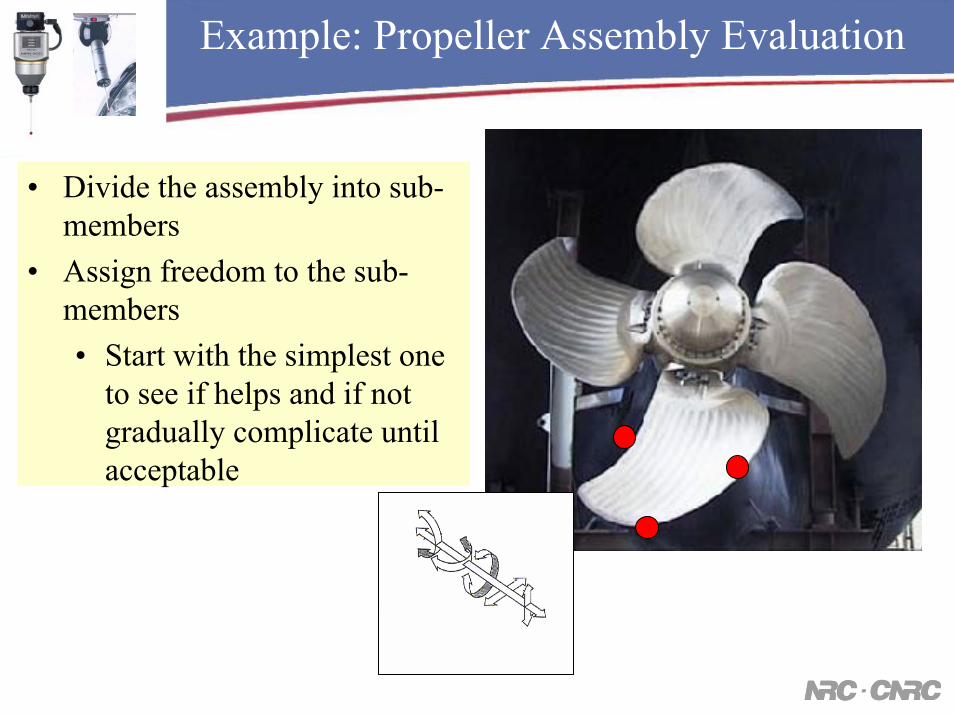
Example: Propeller Assembly Evaluation

• Divide the assembly into sub-members

• Assign freedom to the sub-members• Start with the simplest one

to see if helps and if not gradually complicate until acceptable

Same Data, Different Goal - Different Result

Result 1

Result 2

Result 3

The right software tools are not readily available

Courtesy of Kotem

Best-fitting helps to identify sub-assembly problems

Problem: To find if a sub-assembly member is out of tolerance or only its position in the assembly is not correct

Special Cases

Mathematical Criteria -Combined Requirements

A

B

Airbus A380

Courtesy of Airbus

Best-fit must satisfy the tolerance graph for parameters A B


A

B

Example: Simultaneous requirements for an UNIFORM GAP while keeping parameter Aan B to remain within the tolerance area as

safely as possible


There are cases when some areas (points) may need to be kept in tolerance and at the same time bring others as closer as possible to nominal

Courtesy of Airbus

Comparison of STL Files

Example: a human joint bone is scanned and reverse engineered. The model needs to be compared to the original. There is no CAD model – only STL data.

• Often the result of reverse engineering effort• The same part scanned with different density will

produce different STL file• These are triangulated surfaces and accuracy

depends on the size of the triangles.

Best-fit in CMM software

Mitutoyo Cosmos

Uncertainty Sources for the Best-fitting Process

• Mathematical criterion not reflecting the goal• Local minimum

– Starting position, number of runs– Optimization parameters

• Tolerancing conditions• Weigh factor condition

– Point distribution• Introduced by a data reduction algorithm

• Wrong association of points• Not using the freedom available or using wrong degrees of freedom

– Degrees of freedom on the dub-assemblies– Not be able to use the right constraint

• Outliers• Not excluding points to be fixed• Last but to the least – the human factor (bad judgment , lack of

understanding, etc.)

Best-fitting – The Philosophy

When optimizing a part there are many possible solutions. It is not easy to choose which one is the best. Although we are looking into geometrical dimensions the reality is that our final goal is always an economical one – time, money. Questions like – “How easy is to fix this feature? How expensive, How much time it is going to take?” are most important. A good best-fitting software would have large number of special software tools which will allow you to express what you want. You can control all the degrees of freedom of the part, use weight factors, exclude outliers, use different mathematical criteria, group points or features and allow them degrees of freedom, build non-uniform complex tolerance zones to make a soft-gauge, etc. It takes seconds to perform a “What-if” analysis.

Case Study – DRF Non-fully Constrained

Z

Datums K and M together can constrain 5 degrees of freedom. The rotation about the Z axis is unconstrained.


Circle used for alignment

- Measurement Result

- Tolerance Zone for location

Point out-of-tolerance

In this case, we have a hole #4 out of tolerance, while hole #1, the one we used for alignment has its

tolerance zone unused!

1

2

3

4

Rotation available


15.04 =∆α

05.02 −=∆α

11.03 =∆α 01 =∆α

• Switch to Polar coordinate system

• Measure the holes.• Calculate the average • Rotate coordinate system by that

angle in the opposite direction• In this example by -0.0502

degrees

α∆

Manual Best-Fit

0502.0=∆ AVRα


15.04 =∆α

05.02 −=∆α

11.03 =∆α 01 =∆α

• Switch to Polar coordinate system• Measure the holes.• Calculate the average • Rotate coordinate system by that

angle in the opposite direction• After rotation recalculate hole

centres in Cartesian coordinate system

• Calculate average dX, dY of the hole centres

• Translate by dX, dY average deviation but in opposite direction

• Origin must stay within mobility boundary!

Manual Best-Fit and use of the datum mobility

0502.0=∆ AVRα

α∆

Measurements of a known geometry using material condition approach

There is very significant trend in North America towards using profile tolerance whenever possible.

In fact most of the current tolerances can be substituted with a simple profile tolerance

The concept of MMC, RSF and LMC

GD&T Example

DRF - fully constrained, possible mobility from MMR, LMR

Reproduced from ASME Y14.5M-1994

GD&T – MMC, LMC, RFS

MMC – Maximum Material Condition (Requirement)

LMC – Minimum Material Condition (Requirement)

RFS – Regardless of Feature Size

Try to remember:

• MMC - “Minimum GAP” preservation• Mating parts, assemblies

• LMC – “Minimum Material” preservation• Castings, parts to be machined

• RFS – “Doesn’t matter”

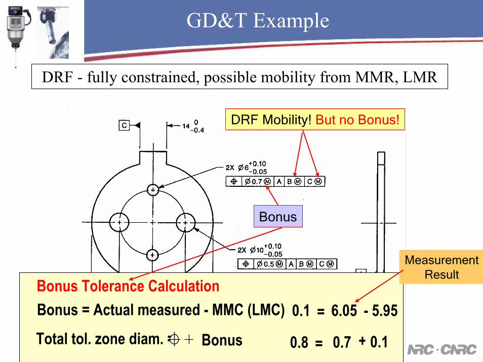
GD&T Example

DRF - fully constrained, possible mobility from MMR, LMR

Bonus

DRF Mobility! But no Bonus!

Bonus = Actual measured - MMC (LMC) sizeBonus Tolerance Calculation

Total tol. zone diam. = Bonus=0.1 6.05 -- 5.95

=0.8 0.7 + 0.1

Measurement Result

DRF Mobility Requires Best-fitting

DRF - fully constrained, possible mobility from MMR, LMR14.0 (MMC)

64.0 (MMC)

Without MMR modifier on the datum this part would be rejected!

14.0 (MMC)

64.0 (MMC)

Mobility!

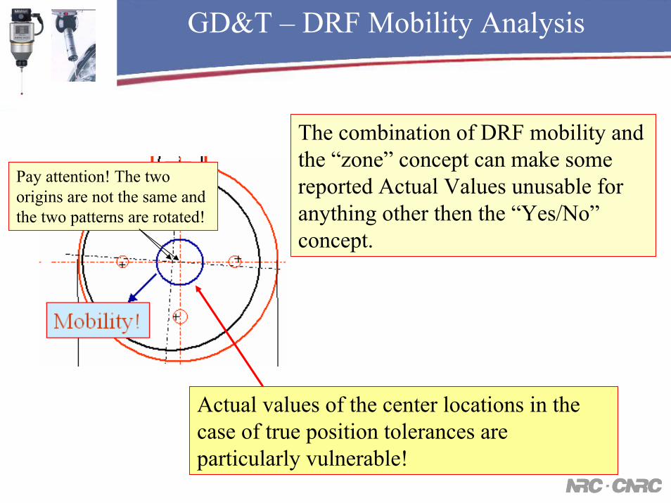
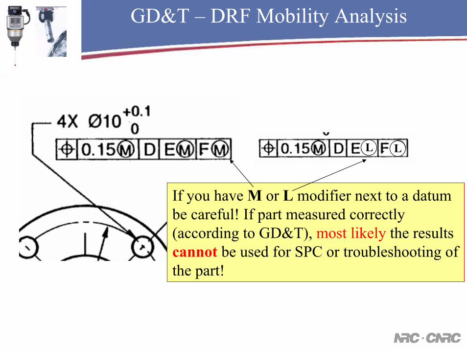
GD&T – DRF Mobility Analysis

The combination of DRF mobility and the “zone” concept can make some reported Actual Values unusable for anything other then the “Yes/No”concept.

Pay attention! The two origins are not the same and the two patterns are rotated!

Actual values of the center locations in the case of true position tolerances are particularly vulnerable!

GD&T – DRF Mobility Analysis

L L

If you have M or L modifier next to a datum be careful! If part measured correctly (according to GD&T), most likely the results cannot be used for SPC or troubleshooting of the part!

Thank You!

Measurements of Free Form Surfaces and Best-fitting ...

Documents

Transcript of Measurements of Free Form Surfaces and Best-fitting ...