Measurements and wall modeled LES simulation of trailing...

aeroacoustics volume 9 · number 3 · 2010 – pages 329–355 329

Measurements and wall modeled LESsimulation of trailing edge noise caused

by a turbulent boundary layer

Björn Greschner1, J. Grilliat2, M.C. Jacob2 and F. Thiele1

1Institut für Strömungsmechanik und Technische Akustik, Technische Universität Berlin,

Müller-Breslau-Str. 11, D-10623 Berlin2Centre Acoustique du LMFA, UMR CNRS 5509 — Ecole Centrale de Lyon —

Université Claude-Bernard Lyon I, F-69134 Ecully Cedex

[email protected], [email protected], [email protected],

[email protected]

Received July 9, 2009; Revised September 18, 2009; Accepted January 18, 2010

ABSTRACTA successful comparison between CFD-CAA and measurements of trailing edge noise is shownfor a highly loaded and cambered NACA 5510 airfoil at a chord based Reynolds number ofaprox. 1 million placed in a quiet low Mach number flow. The simulation is based on a newvariant of the DES - the Improved Delayed Detached Eddy Simulation (IDDES).

The flow is fully attached to the airfoil and therefore only the small turbulent boundarystructures that interact with the trailing edge generate significant broadband noise in the farfield. The IDDES approach is designed to extend the LES region of the original DES approach(hybrid RANS/LES) from Spalart et. al. (1997) to the turbulent boundary layer, as proposed firstby Travin et. al. in 2006. The non-zonal blending occures therefore inside the boundary layer -the RANS model acts as a wall model for the LES. The actual work shows the capabilities of thisnovel approach for the simulation of broadband noise for attached flows. The simulation iscompared to measurements from the EC Lyon including PIV and LDA data around the airfoiland unsteady on-wall pressure measurements near the trailing edge. Far field computations arecarried out by applying the Ffowcs–Williams and Hawkings analogy to the unsteady wallpressure field and compared to acoustic measurements as well as to a far field prediction basedon a trailing edge noise model that is applied to the experimental aerodynamic pressure field.

1. INTRODUCTIONSelfnoise is one of the major noise sources encountered in turbomachinary by-passflows. Although selfnoise is also generated by the outlet guide vanes (OGV) trailingedges, most of the selfnoise is produced by the fan itself due to its high speed motion.Fan selfnoise is generated both at the blade tips as discussed by Jacob et al. [11],Camussi et al. [3] and at blade trailing edges (TE). In [11], the tip noise source is foundto compete with the TE-noise source on a short airfoil and attemps are made to relate

the radiated sound field to unsteady flow mechanisms based on various causalitytechniques [14] including wavelet based approaches following the concepts described inCamussi et al. [4]. Therefore, for long span airfoils, the TE is probably the dominantselfnoise source. In recent years, TE modeling underwent two trends, semi-analyticalmodeling and fully numeric modeling. The semi-analytical approach combines selfnoisebroadband models based on gust theories [1] to RANS input. As discussed by Roger andMoreau in their review paper [23, 22], the analytical modeling of TE–noise is an oldtopic that recently progressed significantly as existing wall pressure spectra models [28]designed for non–zero pressure gradient boundary layers were revisited [9] and [25, 26].As a result, analytical models can now be applied to flow statistics obtained from RANScomputations, assuming convection velocities and spanwise coherence scales.

The fully numerical approach is based on unsteady CFD simulations of the flowfield around the airfoil that is coupled to a time domain acoustic analogy, e.g. theFfowcs–Williams and Hawkings analogy (FWH) or a linearised Euler equations. Thefirst approach was undertaken by Wang et al. [35] with an incompressible LEScomputation of a low Mach number (Ma ≈ 0.1) flow past a controlled–diffusion airfoiland compared to an experimental data set obtained at ECL [21]. Compared to Wang et al.the present investigation shows higher Mach number (Ma ≈ 0.2) and Reynolds number(Rec ≈ 930000) and a compressible Detached Eddy Simulation (DES) is performed.

The Detached Eddy Simulation (DES) approach is based on the idea of combiningRANS and LES turbulence models. It has become increasingly popular in recent years,since DES requires a reduced computational effort in comparison to genuine LES, whileretaining much of the physical accuracy of the LES method. The basic concept of DESwas published in 1997 [32] and was based on the popular Spalart-Allmaras (SA) one-equation turbulence model (accordingly refered to as ‘DES97’). The peculiarity of a DESapproach consists in using a single turbulence model, which behaves like a subgrid-scale model in regions where the grid density is fine enough for a LES, and like a RANSmodel in regions where it is not. The self consistent formulation of this non-zonalapproach is the key benefit in the development of a future ‘every day’ industrial tool.

A number of studies demonstrate advantages of DES over unsteady RANS methodsfor flows with massive separation, e.g. in [12], where the attached boundary layer istreated with the original RANS model and the separated regions with LES. In thepresent self noise configuration only turbulent boundary structures and no detachedflow exists that causes noise, therefore a LES or DNS would be recommended for thesetypes of problems. Therfore the standard DES97 approach is not targeted to producingany reasonable result (in meanings of resolved boundary layer flow), because the useof the LES mode is prohibited in the boundary layer. The new Improved DelayedDetached Eddy Simulation (IDDES) or wall–modelled LES is designed to extend theLES region into the turbulent boundary layer, as proposed first by Travin et al. [33] in2006. With LES-like grids near the wall the non-zonal blending happens therefore insidethe boundary layer — the RANS model acts as a wall model for the LES. The majoradvantage of the IDDES for the simulation of complex problems, e.g. turbomachinaryflows, is an additional degree of freedom in grid generation with respect to LES. One canchoose the area of interest (= major broadband noise source regions) and creates there a

330 Measurements and wall modeled LES simulation of trailing edge noise

caused by a turbulent boundary layer

fine, LES–like grid. In the rest of the domain one is free to coarsen the mesh to aRANS–grid. This clearly demonstrates the advantage of the idea of the non–zonalIDDES approach over the pure LES for complex problems. The basic functionality ofthe IDDES was successfully demonstrated by Travin et al. [33], Shur et al. [31] andat ISTA by Mockett et al. [20, 19] for a wide range of simple cases, such like periodicchannel flows and the backward facing step. The test of the functionality of theIDDES on applied cases with the prediction of broadband noise is the novelety in thepresent investigation.

The paper consists of four parts. The first part contains a brief description of the selfnoise experiment investigated in the EU–project PROBAND by the ECL. The secondpart describes of the numerical basics of the IDDES method including the simulationdetails that are conducted in EU–project PROBAND by ISTA. This is followed by twoseparated sections related to the aerodynamic and aeroacoustic analysis of thesimulation results compared to the experiment.

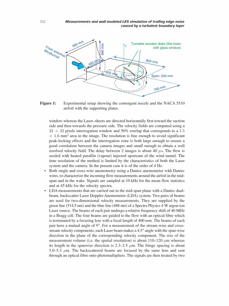
2. FLOW CONFIGURATION AND EXPERIMENTAL SETUPThe experiment is carried out in the anechoic room (10 m × 8 m × 8 m) of theLaboratoire de Mécanique des Fluides et d’Acoustique (LMFA), a joint CNRS-ECL-UCB Lyon-I laboratory located at the Ecole Centrale de Lyon. Air is supplied by a highspeed, subsonic, anechoic wind tunnel at Mach numbers ranging up to 0.3. The set-upis shown in Fig. 1. Before reaching the duct exit, the air is accelerated by a convergentnozzle from a 560 mm × 560 mm cross–section to the 450 mm wide and 200 mm hightest section. In the test section, the air flows as a semi open jet into the core of which aNACA 5510 profile (5% camber, 10% thickness) with a 200 mm chord and 200 mmspan is attached between two horizontal plates. The airfoil is mounted onto a woodendisk, which allows to tuning the angle of attack. A glass window is mounted into thelower plate allowing for PIV and LDA measurements in the vicinity of the airfoil. Thereference velocity at the exit of the wind tunnel is U

0= 70 m/s, and the turbulence level

u′/U0 is about 0.7%.The chord-based Reynolds number is Rec ≈ 930000. For these inflow parameters, the

reference configuration is obtained with an α = 15° angle of attack. This results into ahigh load but the airfoil geometry prevents the flow to separate.

MeasurementsThe experiment was conducted as part of the fan tip flow and noise experimentalcampaign reported in [11] and provided a large data set that will not be described in thepresent paper. Measurements referred to in this paper include:

• PIV measurements in the mid- span plane, with a La Vision system and two fasthigh resolution CCD cameras (1280 × 1024 pixels each) with 35 mm lenses andinterferometric filters. Their axes are normal to the light sheet. The cameras arelocated next to each other in order to provide pictures from a 250 × 105 mm2

rectangular area surrounding the whole airfoil with a good resolution. Images arepost-processed with the Davies software. The cameras are placed beneath the glass

aeroacoustics volume 9 · number 3 · 2010 331

window whereas the Laser–sheets are directed horizontally first toward the suctionside and then towards the pressure side. The velocity fields are computed using a32 × 32 pixels interrogation window and 50% overlap that corresponds to a 1.5

× 1.6 mm2 area in the image. The resolution is fine enough to avoid significantpeak-locking effects and the interrogation zone is both large enough to ensure agood correlation between the camera images and small enough to obtain a wellresolved velocity field. The delay between 2 images is about 40 µs. The flow isseeded with heated paraffin (vapour) injected upstream of the wind tunnel. Thetime resolution of the method is limited by the characteristics of both the Lasersystem and the camera. In the present case it is of the order of 4 Hz.

• Both single and cross-wire anemometry using a Dantec anemometer with Dantecwires, to characterize the incoming flow measurements around the airfoil in the mid-span and in the wake. Signals are sampled at 10 kHz for the mean flow statisticsand at 45 kHz for the velocity spectra.

• LDA measurements that are carried out in the mid-span plane with a Dantec dual-beam, backscatter Laser Doppler Anemometer (LDA) system. Two pairs of beamsare used for two-dimensional velocity measurements. They are supplied by thegreen line (514.5 nm) and the blue line (488 nm) of a Spectra Physics 4 W argon-ionLaser source. The beams of each pair undergo a relative frequency shift of 40 MHzin a Bragg cell. The four beams are guided to the flow with an optical fibre whichis terminated by a focusing lens with a focal length of 400 mm. The beams of eachpair have a mutual angle of 9°. For a measurement of the stream-wise and cross-stream velocity components, each Laser beam makes a 4.5° angle with the span-wisedirection in the plane of the corresponding velocity component. The size of themeasurement volume (i.e. the spatial resolution) is about 110–120 µm whereasits length in the spanwise direction is 2.3–2.5 µm. The fringe spacing is about5.0–5.3 µm. The backscattered beams are focused by the same lens and sentthrough an optical fibre onto photomultipliers. The signals are then treated by two



x

yO

z

560

mm

560 mm

700 mm

450 mm 850 mm

From anechoic

Windtunnel

Span: 200 mm405 mm

Turnable wooden disks (the lowerwith glass window)

Figure 1: Experimental setup showing the convergent nozzle and the NACA 5510airfoil with the supporting plates.

Dantec real-time signal Analysers and post-processed based on 0th order re-sam-pling. The seeding material is the same as that used for the PIV measurements.

• Steady and unsteady pressure measurements on the airfoil and the lower plate,including the gap: the sampling rate is 64 kHz and the time series are long enoughto perform 500 averages of 8192 point FFT’s; this is enough to obtain a statisticalerror of less than about 1–2% on the coherence between 2 signals; the measure-ments are carried out with a remote microphone technique described by Roger andPerennes [24]; the sensors used are B&K type 4935 ICP 1/4” microphones that arepre-amplified by a PXI system; they are connected to the wall measurement 0.5 mmdiameter pinholes via narrow tubes. The probes used specifically for the self-noisemeasurements are located along the mid-span chord mostly on the suction sidedownstream quarter chord of the airfoil (see Fig. 2). Steady pressure probes are notall shown on this figure.

• Far field measurements that are performed in the mid-span plane, at about 1.7 mfrom the airfoil leading edge. For this purpose, two B&K type 4191 1/2” microphonesand B&K 2669 preamplifiers are placed at each side of the airfoil. The microphonesare turned around the airfoil in far field conditions above fmin ≈ 250 Hz.

3. NUMERICAL METHODS AND SETUPIn this section a brief description of the used methods and simulation tools is given.The wall-modeled LES (IDDES) is based on a Compact Explicit Algebraic StressTurbulence Model (CEASM) which is built on a two–equation k – ε model from Lienand Lechziner [17]. The compressible IDDES is used to calculate the unsteady flowfield around the airfoil and the data are feed into a standard Ffowcs–Williams andHawkings (FWH) [8] code for the calculation of the noise in the far field.


1112131415

41 39 38

TE LE

9

Suction side

4 0Mid-span

Figure 2: Unsteady pressure probe locations: suction side probes 11 to 15 arelocated at 97.5% chord respectively at 6 mm, 1 mm, 0 mm, –2 mm and12 mm from mid–span. Probe 41 is facing probe 13. Other probes arelocated at mid–span: probes 9 and 38 are at 77.5% chord on either side ofthe airfoil, probe 39 is at 85% chord on the pressure side and probe 4 isat 25% chord.

3.1. ELAN flow solverThe unsteady, aerodynamic field is computed by using an in–house, finite–volume codethat solves either the unsteady Reynolds–averaged or spatially filtered Navier–Stokesequations employing a RANS or Large Eddy Simulation, respectively. A time implicitformulation is used with second order accuracy both in space and in time. All scalarquantities, as well as the Cartesian components of tensorial quantities are stored in thecell centres of arbitrarily curvilinear, semi–structured grids that can fit very complexgeometries with the desired local refinement level. Linear momentum equations aresolved sequentially, with the pressure field computed at each time step via a separateiterative procedure based on a pressure-correction scheme of the SIMPLE type with anadditional compressible convection term as described by Ferziger & Peric [7]. The setof compressible equations is completed with an equation for the total enthalpy and theideal gas law. A generalised Rhie & Chow interpolation is used to avoid an odd–evendecoupling of pressure, velocity and Reynolds–stress components. The system ofequations is solved by an iterative method, the well known Stone’s SIP solver.

3.2. Improved delayed detached eddy simulationThe DES method was developed for the simulation of separated flows with the treatmentof the entire boundary layer using RANS. This non zonal, hybrid technique wasintroduced by Spalart et al. [32] in 1997 (DES97) for the SA turbulence model in orderto combine the strengths of RANS and LES. The fundamental advantages of this hybridapproach are manifest both in terms of computational costs and of accuracy in theprediction of complex wall bounded flows. Furthermore, the high performance of LESin the outer turbulent regions is maintained in the DES technique. The blending is doneby modifying the length scale LRANS of the turbulence model. This model length scaleis substituted by the DES length scale LDES , that is defined similarly to an implicitfilter in LES:

∆ = max (∆x, ∆y, ∆z ) and LDES = min (lRANS, CDES∆).

The method was later generalised to be applicable to any RANS model by Travin et al.[34]. The further investigations on the DES approach shows some problems for critcalcases, e.g. ‘modeled stress depletion’ (MSD) that can lead to ‘grid induced separation’(GIS) and the activation of the near wall damping terms of the underlying turbulencemodel in the LES regions. These problems are adressed by the development of the DelayedDetached Eddy Simulation (DDES) by Menter et al. [18] in 2004 for the SST–k – ω modeland more generally in 2006 by Travin et al. [33]. In channel simulations with massivlyrefined grids near the walls (LES–like grid) the standard DES97 shows two stackedlogarithmic layers, which causes a significant and unphysical reduction of the frictioncoefficient. This effect is called ‘log layer missmatch’ (LLM). The DDES modificationavoids the the activation of the LES mode inside the boundary layer, it ‘delays’ theswitching to the LES mode into well seperated regions, far from walls. Travin et al.[33, 31] publicated in 2006 a modification of the DDES approach, that has shownpromising results for fully–developed turbulent channel flows. This variant is known as



‘improved DDES’ (IDDES) and has been implemented and validated at the ISTA SAEand CEASM DDES variants by Mockett [20]. The major advantage over the formerDES variants is the possibility to simulate resolved turbulent boundary layer structures.It is therefore used in the present study.

The IDDES approach uses a more complex formulation for evaluating the grid filter∆ and for the blending of the grid filter with the RANS turbulent length scale (LRANS ).The grid filter depends additionally on the wall normal distance dw and the height of thecell in wall normal direction hwn:

∆ = min (max [Cwdw, Cwhmax, hwn], hmax) and hmax = max (∆x, ∆y, ∆z ) (1)

Here Cw is a model constant. The blending is done by a so called ‘hybrid function’fhyb, that includes the functionality of former developed DDES (fd) with the shieldfunction Ψ and formulates the modified length scale l

~as follows:

l~

= fhyb (1 + frestore)LRANS + (1– fhyb)LLES (2)

with

LLES = CDES Ψ∆ and fhyb = max{(1 – fd), fstep} (3)

The functions fd, frestore, fstep and Ψ are defined in a complex manner by analysis ofthe local boundary layer flow paramters. The complete description of the IDDESapproach is presented in [33, 31].

IDDES of a fully turbulent periodic channel flowThe advantage of this IDDES approach is demonstrated here for a turbulent, 3D, periodicchannel flow at Reτ = 2000. The standard DES of this configuration both on coarse andfine grids always tends to a simple RANS solution without resolving turbulence. If oneforces the solution to resolve the turbulence, the DES shows a typical log–layermismatch (LLM) with an incorrect prediction of the friction coefficient. The IDDESreproduces the correct behavior independent from the grid resolution with resolvedturbulence on fine grids. In Fig. 3 the results of the EASM-IDDES for Reτ = 2000 andubulk = 22.4 m/s with the channel half height of H/2 = 1.0 m on different grids aresummarized. The basic grid is designed as a LES grid for the Reynolds number Reτ = 400,with a wall normal grid size of y+ < 0.5 and a wall tangential resolution in stream wisedirection of ∆x = ∆z · 2 with ∆z+ < 20. The initial field is composed of the resultof a precurser 2D-RANS added with the resolved turbulence of the DIT case (decay ofisotropic turbulence). A slice through the domain is shown with the x-component ofthe velocity on the left side of Fig. 3(a) for three different stream-wise grid resolutions.From top to the bottom, the LES–like grid (∆x = 2 · ∆z), the intermediate grid (∆x = 8 · ∆z) and a RANS-type grid with high aspect ratio cells (∆x = 32 · ∆z) areshown. The differences are obvious. The coarsest grid shows a RANS solution, whereasthe finer grids show resolved turbulence in the core of the channel. The blending


between the RANS an the LES mode happens inside the turbulent boundary layer, thatis depicted in the left plot of Fig. 3(b). In this plot the blending function fhyb (red color)and the resulting model length scale l~ (normalized with the RANS length scale LRANS ,black color) are shown. For the LES-like grid more than 92% of the channel is in the



Figure 3: IDDES of turbulent periodic channnel flow at Reτ = 2000 — demon-stration of wall modeling LES capabilities of the CEASM IDDES ondifferent grids.

LES mode, for the intermediate grid approximately 75% is in the LES mode and thecoarse grid simulation is only in RANS mode. The analysis of the boundary layer u+ = f(y+)–profiles in Fig. 3(b) rigth shows for all grids very good results comparedto the DNS from Hoyas et al. [13]. Therefore the IDDES shows consistent resultsindependent of the near wall grid resolution for the fully turbulent periodic channel flow.

3.3. FWHBased on the work of Lighthill [16] and Ffowcs–Williams and Hawkings [8], theunsteady pressure and velocity fluctuations in the flow field constitute the sources ofan inhomogeneous wave equation governing the noise propagation problem. Thesefluctuating values can be derived from unsteady CFD. The equation used for computingthe acoustic far field at different observer positions based on Farassats formulation 1A [6]for penetrable surfaces reads as follows:

with

where [·]ret denotes quantities that have to be evaluated at retarded time τ = t – r/a.In this equation, all terms on the right hand side represent sources located on thesurface, the term representing the volume sources (Lighthill term) is neglected. Inreference [10], it is shown on a rod-airfoil test case that for low Mach number flowssuch as the present one, this assumption is justified in cases: either the integrationsurface coincides with the solid boundaries or it surrounds all the perturbationsgenerated by the flow. The program C3Noise used for acoustic prediction is an in–housedeveloped code and has been validated by Eschricht et al. [27, 29] for configurations ofrigid and penetrable surfaces.

3.4. Numerical setup and gridThe flow conditions used for the compressible simulation are set according to theexperiment. The mean inflow velocity is Uin = 70.204 m/s at angle of attack of α = 7°.This inflow angle is quite different with respect to the experiment (15°) due to fact thatfor the CFD a homogeneous inflow field is used instead of the open jet configuration in

U vu

K rM aM aMn nn

r r=

+ = +1 – –

�

�

�

�0 0

& 22 Mva

L L M Lx y

rL L u u v P

rr

M i i ri

i i i n n i

=

= = = +( – )

( – )� nn

in i ijP p p n r x y p a= = ′ = ′( – ) | | – |0

2τ neglectedr r

�

41

2π ′ =

+

p x tU U

r Mn n

r ret

( , )( )

( – )

r &&

�0 ddS

U K

r MdS

aL

n

r retss

r

+

+

∫∫�

0

2 31

1

( – )

&

rr MdS

L L

r Mr rets

r M

r( – )

–

( – )1 12 2 2

+

∫

+

∫rets

r

r r

dSa

L K

r M1

12 3( – )

eets

dS∫


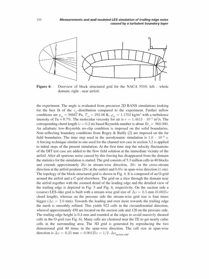
the experiment. The angle is evaluated from precursor 2D RANS simulations lookingfor the best fit of the cp–distribution compared to the experiment. Further inflowconditions are pin = 98667 Pa, Tin = 292.06 K, �in = 1.1702 kg/m3 with a turbulenceintensity of Tu = 0.7%. The molecular viscosity for air is v = 1.4613 · 10–5 m2/s. Thecorresponding chord length (c = 0.2 m) based Reynolds number is about Rec = 960.000.An adiabatic low-Reynolds no-slip condition is imposed on the solid boundaries.Non–reflecting boundary conditions from Bogey & Bailly [2] are imposed on the farfield boundaries. The time step used in the aerodynamic simulation is 1.0 · 10–6 s. A forcing technique similar to one used for the channel test case in section 3.2 is appliedto initial steps of the present simulation. At the first time step the velocity fluctuationsof the DIT test case are added to the flow field solution at the immediate vicinity of theairfoil. After all spurious noise caused by this forcing has disappeared from the domainthe statistics for the simulation is started. The grid consists of 5.3 million cells in 40 blocksand extends approximately 26c in stream-wise direction, 20c in the cross-streamdirection at the airfoil position (29c at the outlet) and 0.05c in span-wise direction (1 cm).The topology of the block-structured grid is shown in Fig. 4. It is composed of an O-gridaround the airfoil and a C-grid elsewhere. The grid on a slice through the domain nearthe airfoil together with the zoomed detail of the leading edge and the detailed view ofthe trailing edge is depicted in Fig. 5 and Fig. 6, respectivily. On the suction side a(coarse) LES–like grid is built with a stream-wise grid size of ∆z = 0.5 mm (0.0025cchord length), whereas on the pressure side the stream-wise grid size is four timesbigger (∆z = 2.0 mm). Towards the leading and even more towards the trailing edgethe mesh is smoothly refined. This yields 922 cells in the circumferential direction,whereof approximately 450 are located on the suction side and 120 on the pressure side.The trailing edge height is 0.4 mm and rounded at the edges to avoid massivly shearedcells in the O-grid (see Fig. 6). Many cells are clustered near the TE to get nearly cubiccells in the surrounding area. The 3D grid is generated by reproducing the twodimensional grid 40 times in the span-wise direction. The cell size in span-wisedirection is ∆z = 0.25 mm = 0.00125c = 1/2 · ∆xsuction side.



Figure 4: Overview of block structured grid for the NACA 5510: left - wholedomain; right - near airfoil.

On the complete airfoil the first cell size normal to the wall is in turbulent units y+ < 0.4

with a peak value of y+ ≈ 0.65 at the stagnation point (see Fig. 7). The correspondingstream- and span-wise grid resolution are around ∆x+ ≈ 100 (black curve withoutsymbols) and ∆z+ ≈ 50 (red curve without symbols) for the suction side as depictedin Fig. 7 right. The pressure side shows a quite coarser stream-wise resolution with∆x+ up to values of 270, but small values for the span wise turbulent grid size of 20 <∆z+ < 40 (black and red curve with symbols). Hence we have a relative coarse LES–likegrid on the suction side and a fine RANS–like grid on the pressure side, a quitechallenging task for a LES wall model.

4. AERODYNAMICSThe IDDES simulation of the flow around the NACA 5510 airfoil shows a resolvedturbulent boundary layer on approximately 90% of the suction side. On the otherhand, the pressure side remains in RANS mode. In Fig. 8, a snapshot of the resolvedvortex structures is shown by isosurface of the λ

2–criterion coloured by the velocity

magnitude. The domain is mirrored on the front- and back-side in spanwise direction.On the midspan plane, the time derivative of the pressure is also plotted in shades ofgrey. This provides a view of the aeroacoustic source regions and the wave propagation


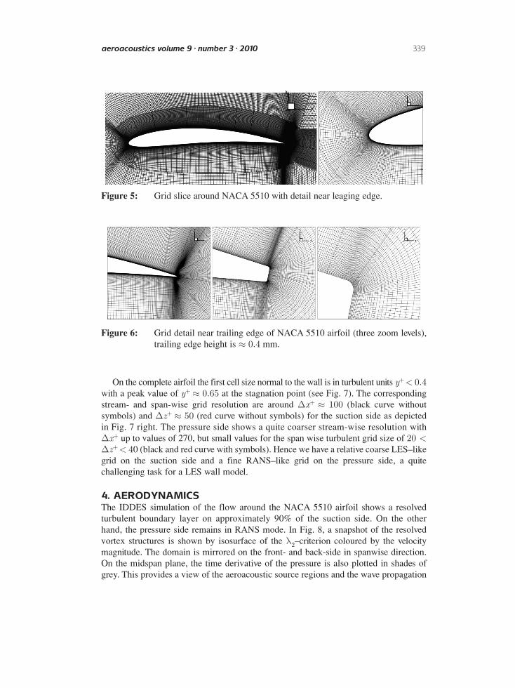
Figure 5: Grid slice around NACA 5510 with detail near leaging edge.

Figure 6: Grid detail near trailing edge of NACA 5510 airfoil (three zoom levels),trailing edge height is ≈ 0.4 mm.



0.8

1

0.6

0.4

0.2

00 0.2 0.4 0.6

x/c

y+

0.8 1

50

100

150

200

250

300

00 0.2 0.4 0.6

x/c

∆x+

, ∆z+

0.8 1

∆x + top∆x + bottom∆z+ top∆z+ bottom

y+ topy+ bottom

Figure 7: Non dimensional grid spacing: left − y+ (normal to wall); right − ∆x+

and ∆z+ (stream wise and span wise direction); averaged over 8000time steps.

Figure 8: Visualization of vortex structures by a λ2–isosurface coloured with the

velocity magnitude (domain is mirrored in span-wise direction at frontand back side), the time derivative of the pressure is given on a 2D cut inshades of gray to visualize the waves propagating away from the airfoil.

in the near field of the airfoil as computed by the compressible CFD-solver. On thesuction side, the flow is laminar near the stagnation point. At 10% chord length themassivly sheared viscous flow becomes unstable at the outer edge of the boundary layerand immediately breaks up into small structures due to the flow deceleration. Thevelocity magnitude is still over 110 m/s (≈ 1.6 × Uin , red color) in this transitionalregion. The resolved, turbulent boundary-layer structures travel downstream with adecreased convection velocity into the direction of the trailing edge. The mean flow isgenerally attached near the trailing edge but shows some events with recirculating flow.Therefore, the size of the stuctures grows massively at the TE.

There are no resolved boundary layer structures on the pressure side in the simulation– no structures are visible by the λ

2–criterion. The major acoustic source region is

located near trailing edge. A secondary source region can be observed near leadingedge, shortly after the transition due to the accelerated vortical structures. The frequencyof this pressure fluctuation is very high (≈ 20 – 40 kHz) with sound pressure levels morethan 20 dB lower than the TE noise, which is not surprising since there is nogeometrical singularity nearby. The normalized z-component of the vorticity ωzc/u isdepicted in Fig. 9. The difference between the boundary layer on the suction andpressure side is obvious: On the pressure side the boundary layer (BL) is in RANS-mode, visible by the highly positive and homogeneous values of ωzc/u (red color). At75% chord lenght the transition to turbulence can be recognized by the growing of theBL thickness. There is a similar thin homogeneous viscous layer in RANS mode on thesuction side on the first 10% of the profile, but with negative levels for ωzc/u. After thatpoint, one can observe mixed areas with positve and negative values in the BL, that canhappen only in resolved flows. To determine the blending position between the RANS-and LES-mode the blending function fhyb is shown in Fig. 10 in two different plots. Thevalue of fhyb is one in the full RANS-mode and zero in the LES-mode. The upperpicture of Fig. 10 shows the same λ

2–isosurface as Fig. 8 now coloured with the

blending function. Here the vortical structures in the turbulent boundary are in the LES-mode, clearly visible by the red color (fhyb = 0), but one can still recognize the thin, bluearea near the airfoil – the viscous layer is in RANS-mode on the suction side. Therefore,the blending occurs inside the boundary layer. In Fig. 10 bottom fhyb is dipicted on amid-span plane, but with reversed color scale with respect to the former plot; red color


−17 −13 −9 −5 −1 3 7 11 15

Y

Z Xωzd/u0 :

Figure 9: Normalized vorticity ωzc/u on a mid-span plane.

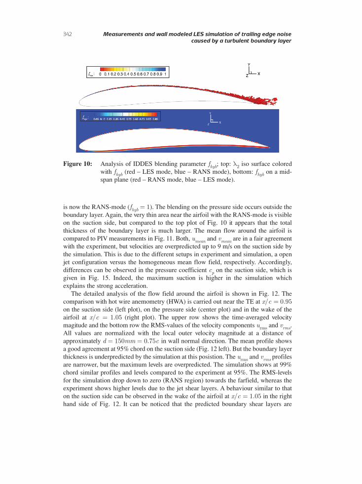
is now the RANS-mode (fhyb = 1). The blending on the pressure side occurs outside theboundary layer. Again, the very thin area near the airfoil with the RANS-mode is visibleon the suction side, but compared to the top plot of Fig. 10 it appears that the totalthickness of the boundary layer is much larger. The mean flow around the airfoil iscompared to PIV measurements in Fig. 11. Both, umean and vmean are in a fair agreementwith the experiment, but velocities are overpredicted up to 9 m/s on the suction side bythe simulation. This is due to the different setups in experiment and simulation, a openjet configuration versus the homogeneous mean flow field, respectively. Accordingly,differences can be observed in the pressure coefficient cp on the suction side, which isgiven in Fig. 15. Indeed, the maximum suction is higher in the simulation whichexplains the strong acceleration.

The detailed analysis of the flow field around the airfoil is shown in Fig. 12. Thecomparison with hot wire anemometry (HWA) is carried out near the TE at x/c = 0.95

on the suction side (left plot), on the pressure side (center plot) and in the wake of theairfoil at x/c = 1.05 (right plot). The upper row shows the time-averaged velocitymagitude and the bottom row the RMS-values of the velocity components u

rmsand vrms.

All values are normalized with the local outer velocity magnitude at a distance ofapproximately d = 150mm = 0.75c in wall normal direction. The mean profile showsa good agreement at 95% chord on the suction side (Fig. 12 left). But the boundary layerthickness is underpredicted by the simulation at this posistion. The u

rmsand vrms profiles

are narrower, but the maximum levels are overpredicted. The simulation shows at 99%chord similar profiles and levels compared to the experiment at 95%. The RMS-levelsfor the simulation drop down to zero (RANS region) towards the farfield, whereas theexperiment shows higher levels due to the jet shear layers. A behaviour similar to thaton the suction side can be observed in the wake of the airfoil at x/c = 1.05 in the righthand side of Fig. 12. It can be noticed that the predicted boundary shear layers are



Figure 10: Analysis of IDDES blending parameter fhyb; top: λ2

iso surface coloredwith fhyb (red – LES mode, blue – RANS mode), bottom: fhyb on a mid-span plane (red – RANS mode, blue – LES mode).

smaller, but with higher RMS-values. The boundary layer of the pressure side is muchsmaller near the TE than on the suction side, which is clearly visible in the wake (rightplot of Fig. 12) and in the center plot of Fig. 12. In Fig. 13, the boundary layer profilesalong the airfoil are depicted for the suction (left) and the pressure side (right). Thismean profiles were obtained during the last 37000 time steps (T = 0.037 s). Theprofiles shown, are normalized by the wall-parallel velocity at a distance d/c = 0.125

– the normalization velocities for every position are summarized on the top the picture(red numbers). At 10% chord the maximum outer velocity is about 76% higher than thefree stream velocity. For the suction side the wall-parallel velocity component profilesu show a fast increasing boundary layer thickness downstream of 50% chord (x/c = 0.5),due to the strong adverse pressure gradient on the airfoil. Downstream of 90% chord the

flow tends to be close to seperation, but it is still attached . On the pressure

side the boundary layer thickness is smaller and shows between the stagnation point andmore than 50% chord a fully viscous behaviour. After that point transiton to turbulencecan be observed. The maximum velocity on the pressure side is less than the freestreamvelocity (u||

max/u0

= 0.94 at x/c = 0.9). Fig. 14 depicts some selected boundary layerprofiles in a logaritmic scale for the suction side (left plot) and the pressure side (rightplot). The non-dimensional u+ = f(y+) profiles show a detailed view of the blendingbehaviour inside the turbulent boundary layer. The symbols flag the position of fhyb =0.5. On the suction side for 10% chord one can see a typical viscous boundary layer

∂

u∂y

positive


Figure 11: Comparison of PIV (left) and IDDES (right) of the averaged velocity u- and v-component around the airfoil; top row – u-velocity, bottom row –v-velocity.

with blending outside the boundary layer (orange curve). At 25% (black) and 50% chord(green) the typical combined viscous and logarithmic laws of the wall can be recognizedin the velocity profiles. The blending to the LES-mode occurs inside of the boundarylayer at approximately y+ ≈ 60. At 80% (brown) and especially 97.5% chord (blue)strong degenerated profiles are found, due to the strong adverse pressure gradient. At thelast position the blending occurs around y+ ≈ 18 (see blue curve). The pressure sideshows a completely different behaviour. At 10% (orange), 25% (black) and 75% chord(brown curve) the profiles have the typical shape of a viscous boundary layer and theblending to LES occurs outside of the BL. Near the trailing edge at 97.5% (blue curve)and 100% chord (green curve) the blending takes place in the logaritmic layer and tendsto move into the viscous boundary layer. Only for these two profiles, the blendingfunction is nearly constant (fhyb = 0.5) from the marked positions (blue and greensquare) to the outer part of the boundary layer. Therefore it is not a real LES-mode inthe outer part of the boundary layer at these positions – the resulting turbulent lenghtscale in the model is only slightly decreased due to the constant blending of fhyb = 0.5.The last part of this section is related to statistics of the force coefficients and wall



80

60

Dis

tanc

e [m

m]

40

20

00 0.2

100

0.4 0.6Normalized averaged velocity

0.8 1 1.2

avg. vmag

, HWAavg. v

mag, IDDES

Dis

tanc

e [m

m]

00 0.05

30

25

20

15

10

5

0.1 0.15

Dis

tanc

e [m

m]

Dis

tanc

e [m

m]

00 0.05

30

25

20

15

10

5

0.1 0.15urms/uII

max, vrms/uIImax urms/uII

max, vrms/uIImaxurms/uII

max, vrms/uIImax

Dis

tanc

e [m

m]

−150.05

−10

−5

0

5

10

15

20

0 0.1 0.15

20

0

Dis

tanc

e [m

m]

−20

−40

0 0.2

40

0.4 0.6 0.8 1 1.2Normalized averaged velocity

avg. vmag

, HWAavg. v

mag, IDDES

80

60

40

20

00.4 0.6

100

0.8 1 1.2Normalized averaged velocity

avg. vmag

, HWAavg. v

mag, IDDES

urms

, HWAv

rms, HWA

urms

, IDDESv

rms, IDDES

urms

, HWAv

rms, HWA

urms

, IDDESv

rms, IDDES

urms

, HWAv

rms, HWA

urms

, IDDESv

rms, IDDES

Figure 12: Comparison of normalized averaged velocity and RMS-values of velocitycomponents to HWA measurements near TE (x/c = 0.95) on suction side(left) and pressure side (middle) and in the wake at x/c = 1.05 (right);top row averaged vmag and bottom row urms, vrms, (symbols – HWA, lines– IDDES), normalizition with outer velocity magnitude u||

max.

pressure spectral analysis including spanwise coherence determination. In Fig. 15 theaveraged pressure coefficient cp on the airfoil of the simualtion is compared to theexperimental data. Whereas the pressure side shows a good aggreement, the differenceson the suction side are obvious. Again this is due to the different setups in experimentand simulation, an open jet configuration and the homogeneous mean flow field,respectively. As mentioned above, velocities are higher in the simulation on the suctionside. On the left plot of Fig. 17 the time history of the lift cL, drag cD and the sidecoefficient cS is depicted whereas the associated Power Spectral Density analysis isshown on the right plot. The lift has a mean value of about cL

mean ≈ 1.347 withfluctuation of about ∆cL = ±0.01. The drag fluctuations are about one order ofmagnitude smaller (cD

mean ≈ 0.015 with ∆cD = ±0.002), whereas the side coefficientfluctuates around zero with maximal values of ∆cS = 2.10–5. All curves are broadbandas illustrated by the spectral analysis in the right plot of Fig. 17. The PSD showbroadband spectra with a roll-off at 3 kHz with slight tonal peaks at 420 Hz and 800 Hz.


0.04

x/c = 0.1 x/c = 0.25 x/c = 0.4 x/c = 0.5 x/c = 0.6 x/c = 0.7 x/c = 0.8 x/c = 0.9 x/c = 0.95x/c = 0.975x/c = 0.99x/c = 1.0

0.03

d/c

0.02

0.01

021

1.76

3u ||/uouter + 10x/c uouter ---u || velocity in distance d/c = 0.125

1.59

4 5

1.53

6

1.49

7

1.37

8

1.28

9

1.23

10

1.21

11

1.191.171.14

12

1.14u||max/u0 =

x/c = 0.1 x/c = 0.25 x/c = 0.5 x/c = 0.75 x/c = 0.9 x/c = 0.95x/c = 0.975x/c = 1.0

0.015

d/c

0.01

0.005

021

0.75

3u ||/uouter + 10x/c uouter ---u || velocity in distance d/c = 0.125

0.80

4 5 6

0.76

7 8 9

0.93

10

0.94

11

0.93 0.93 0.92

12

u||max/u0 =

Figure 13: Boundary layer profiles u for different chord-wise positions normalizedwith outer velocity (u

max); top – suction side, bottom – pressure side,statistic based on 37000 time steps (0.037s).



60

50

40

30

20

0100 101 102

y+

u+

103

Symbols: fhyb = 0.5

10

x/c = 0.975

x/c = 0.1 x/c = 0.8

x/c = 0.5x/c = 0.25

0100 101 102

y+

u+

103

Symbols: fhyb = 0.5

10

20

30

40

x/c = 0.975

x/c = 0.1

x/c = 0.75

x/c = 1.0

x/c = 0.25

Figure 14: Non dimensionsional boundary layer u+ = f(y+) profiles on suction andpressure side, the symbols are to flag the blending between RANS andLES mode by fhyb = 0.5; left – suction side, right – pressure side, statisticbased on 37000 time steps.

4

3

2

1−C

P

0

−1

−20 0.2 0.4 0.6

x/c0.8 1

CP exp.CP IDDES

Figure 15: Pressure coefficient cp averagedover 8000 time steps.

13.8

13.6

13.4

Cor

rect

ion

[dB

]

13.2

13

12.8

200 1000 10kf [Hz]

50k

Long span correction based on position x/c = 0.95 (Kato)

Figure 16: Long span body correction foracoustic based on the coherence lenghtanalysis.

The analysis of the pressure fluctuations near the trailing edge is the link to the acousticfield for this configuration, because the vortical structures generate more noise as theypass nearby the TE than elsewhere. Following this, the on-wall pressure spectra at 95%chord in Fig. 18 left shows good agreement with the experiment and this lets anticipatesimilar matching for the acoustic far fields. The predicted levels are about 5–7 dB toohigh over a wide frequency range, but the spectral shape is very similar, except in thelow frequency range for less than 400 Hz. The comparison of the predicted spanwisecoherence length to the measured one in Fig. 18 (right plot) shows good agreementfrom 600 Hz to 5 kHz (maximum frequency of experimental data). In this range offrequencies the coherence length (Lcoh) is less than 6 mm. At low frequencies theexperimental coherence length is very large, which indicates the presence of a completelydifferent flow feature, that can not be reproduced by the simulation. The simulated spanof 10 mm (LS = 0.05c) is less than the span of the test configuration (Lexp= 1.0c),therefore a scaling correction based on the coherence length analysis has been applied,as suggested by Kato [15]. A new version, combining the three formulas of Kato, of thiscorrection formula between the acoustic and simulated sound pressure levels is chosenhere as proposed by Seo et al. [30]. This yields a constant correction of 13 dB withpeaks of 13.4 dB to 13.5 dB at 1500 Hz and 800 Hz, respectively (see Fig. 16). Thecorresponding coherence length at these frequencies levels is about Lcoh ≈ 5 mm, whichis approximately the half of the simulated span.

5. AEROACOUSTICSThe compressible flow simulation has to cover the near field aeroacoustic radiationand refraction effects. The unsteady flow field data are recorded on control surfaces andfed into a FWH analogy tool, as mentioned in section 3.3. A snapshot of the pressure

perturbation p′ and its time-derivative is shown on the left plot of Fig. 19 in the∂pt∂


Figure 17: Drag, lift and side coefficient; left: time history, right: power spectraldensity.

mid-span plane of the simulated domain. The major acoustic source area near thetrailing edge (TE) is clearly visible. The vortical structures in the turbulent boundarylayer pass the TE and generate sound. A second sound source is visible in the pressuretime-derivative in the right plot of Fig. 19 near the leading edge on the suction side. Thissound source is due to the massively accelerated vortex structures near the leading edge.As mentioned in the previous section the frequency of this sound source is very high(more than 10 kHz) and is highlighted by this kind of post-processing (time derivative)– its SPL-level is 20 dB to 30 dB lower than of the TE noise, it is therefore not visiblein the pressure perturbation in the left-hand side.

5.1. Far-field resultsFollowing the experiment, the far-field sound is computed for 47000 time steps (≈ 0.047 s)at a distance of R = 1.7 m from the leading edge of the airfoil. The results from thesimulation are rotated to the experimental angle of attack of 15°. The zero angle isaligned with the mean flow direction of the experiment, with positive angles on thesuction side (counter clock wise). Measurements are available for angles from α = ±35°to α = ±145° with 5° step. The control surface for the FWH analogy is the airfoil wallsurface ‘s001’. Therefore, only the pressure is recorded and used for the calculation ofthe far-field sound.

The far-field sound is calculated for observers from 0° to 360° with a step of 2° andcompared to the experiment and the semi-analytical trailing edge noise model fromRoger and Moreau [23, 22] and Rozenberg et al. [26]. This model is based on Amiet’sTE-model for a semi-infinite chord flat plate [1] — it has been extended to finite chordlenght airfoils and 3D oblique pressure gusts.



x/c = 0.95, exp.x/c = 0.95, IDDES

110

100

90

80

PS

D [d

B]

f [Hz]

70

60

50

40103 104

On wall pressure spectra

0.012

0.008

0.004

L coh

[m]

f [Hz]

0200 103 104

x/c = 0.95, exp.x/c = 0.95, IDDES

Figure 18: On wall pressure fluctuations near TE (x/c = 0.95 ): left – PSD spectraat midspan compared to experiment; right – coherence length Lcoh in spanwise direction.

The input of this model can be obtained from the pressure field near the trailing edgefar enough upstream to be unperturbed by the trailing edge. In practice, wall pressurestatistics (spectrum, span-wise coherence and convection velocity) at approximately 97%chord are required to predict the farfield spectrum. For cambered airfoils or at significantangles of attack, the BL undergoes a streamwise pressure gradient which also modifiesthe wall pressure statistics over short distances. This makes the choice of the optimalchordwise position more difficult and results in significant dispersion of the predicted farfield spectra. A more recent extension of this model [25] related the wall pressurespectrum at a given chord-wise position to the local boundary layer velocity profilefollowing the ad hoc approach of Goody [9] based on Coles, non-zero pressure gradientBL model [5]. This additional wall pressure modelling allows computing TE noise fromRANS computations which don’t provide any statistics from wall pressure. In the presentcase, the far field is computed from the available measured wall pressure statistics. In allplots this model is represented by the acronym TE-model.

The far-field spectra and directivity analysis are plotted on Figs. 20 and 21 : ThePower Spectral Density (PSD) is expressed on a dB scale with reference 4 · 10–10 Pa2

Hz. The spectra of the simulation are calculated by a FFT with 8192 samples with 50averaging which yields a frequency resolution of ∆fsim ≈ 122 Hz, whereas theexperiment uses ∆fexp ≈ 7.8 Hz and the TE-model ∆fTE–model = 100 Hz. On subplot20(a) results from the suction side are plotted whereas subplot 20(b) shows thecorresponding pressure side results. In the centre plots of Fig. 20 that correspond to thecross-stream directions, a good agreement between the experimental data (red dots) andthe fully numerical (CFD-CAA) prediction (black line) is reached between 1 and 5 kHz.Outside of this frequency domain the experiment outranges the computation. At lowfrequencies, the high experimental values might be explained by installation effects but


Figure 19: Snapshot of pressure perturbation p′ (left) and time derivative of

pressure .∂pt∂

also by the underestimate of the spanwise coherence obtained from the CFD. At highfrequencies, the reason is not clear, but since background noise was found to besignificantly lower in the experiment for these frequencies, the discrepancy might be dueto errors of the numerical estimate due to the relatively short simulation time. Similarconclusions might be drawn from the left and right plots obtained at low and highobserver angles respectively.

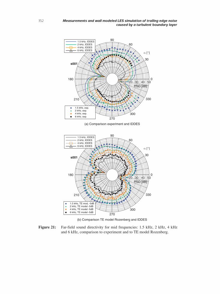
As for the TE model, the results are quite surprising: the model fits very well to theCFD-CAA data between 1 or 2 kHz and say, 10 kHz for most observer angles but fitsmuch better with the experimental results at low frequencies (except at 310°). Evidenceof this is also clear from Fig. 21 where the directivity diagrams obtained from the fullynumeric and the TE-model predictions are compared at various frequencies. Thiscomparison also shows the characteristic dipole pattern of a compact airfoil at lowfrequencies with additional lobes appearing as the frequency increases. For frequenciesand angles at which the numerical and the experimental data collapse, the model alsogives remarkable results.

From these results, it seems that the CFD-CAA approach clearly underestimates thelow frequency part, whereas the model and the CFD-CAA approach collapse the highfrequency part of the sound spectra which they both seem to underestimate. These



Figure 20: Far-field sound for different observers compared to measurements (red)and TE model from Rozenberg (blue circle).

differences might be due to the fact that the experimental and numerical flowconfigurations are quite different and that the far-field estimate is very sensitive to the wallpressure data as can be concluded from a comparison of data sets from literature.Nevertheless, the excellent agreement between the CFD-CAA approach and the TE modelapproach proves that the fully numeric approach is very consistent. Their quite good fittingwith the measured far field gives confidence into both predictions. This implies that theaerodynamic data set is accurate enough to make reliable far field predictions and that theTE noise model can be applied to higher Mach numbers and thicker airfoils than it hadbeen so far. The major restriction in the results can be observed in the low frequency area,due to the short simulation time and the low span-wise extent. Another improvementwould be to apply the TE-model directly to the wall pressure field obtained from thesimulation in order to evaluate the model against the FWH approach. This would requirelong CFD time series as well as a larger span-wise dimension of the CFD domain in orderto compute more accurately the span-wise coherence.

6. CONCLUSIONThe novel IDDES approach was successfully applied to the direct simulation of trailingedge noise of an airfoil. The NACA 5510 airfoil at a high angle of attack and a Reynoldsnumber of one million shows a fully attached turbulent boundary layer, whereupon itsvortical structures interact with the trailing edge and generate sound.

The IDDES is an extension of the standard hybrid RANS/LES Detached EddySimulation method (DES) with the capability to resolve the turbulent boundary layerstructures, if fine, LES-like meshes are used in the area of interest. The direct simulationof the trailing edge noise of the NACA 5510 airfoil, using the IDDES method, showsthe expected performance. A mesh of approximately 5.3 million cells is used tosimulate a span-wise extent of 5% of the chord. On the suction side a fine mesh is used.On the pressure side a four times coarser mesh is used, because no relevant structuresare expected here. The outcome of this is that more than 90% of the boundary layer onthe suction side is in LES mode. On the contrary, the pressure side is fully in RANSmode. The turbulent structures on the suction side are transported to the trailing edge.The detailed analysis of the flow, statistics and spectra near the trailing edge show agood agreement with the experiment. Over a wide range of frequencies the far-fieldsound results are very close to the theory, that uses the measured on-wall spectra,coherence length and pressure gradient near the TE. The major restriction in the resultscan be observed in the low frequency area (≤ 500 Hz).

The IDDES approach is successfully applied to this complex configuration andshows the capability for the simulation of complex, applied cases, e.g turbomachinaryflows. The ability to reproduce resonable results on meshes of different fineness is themajor advantage of the IDDES. With the use of fine meshes in the area of interests, i.e. wallboundary layer, the user has the possibility to get a direct simulation of the noisegeneration mechanism, as shown here for the direct simulation of trailing edge noise.On the other hand the use of coarser grids elsewhere can reduce the computational costsin respect to a LES. To conclude, the IDDES should be further investigated, to get avalid basis for the implementation in industrial turbomachinary simulation tools.




1.5 kHz, IDDES2 kHz, IDDES4 kHz, IDDES6 kHz, IDDES

1.5 kHz, TE mod, -5dB2 kHz, TE model -5dB4 kHz, TE model -5dB6 kHz, TE model -5dB

9060

30

330

0

PSD [dB]

300

270

(b) Comparison TE model Rozenberg and IDDES

210

180

s001

α [°]

0 10 5020 30 40

1.5 kHz, IDDES2 kHz, IDDES4 kHz, IDDES6 kHz, IDDES

1.5 kHz, exp.2 kHz, exp.4 kHz, exp.6 kHz, exp.

9060

30

330

0

PSD [dB]

300

270

(a) Comparison experiment and IDDES

210

180

s001

0 10 5020 30 40

α [°]

Figure 21: Far-field sound directivity for mid frequencies: 1.5 kHz, 2 kHz, 4 kHzand 6 kHz, comparison to experiment and to TE model Rozenberg.


ACKNOWLEDGEMENTThis study is a part of the EU funded 6th Framework project PROBAND n° AST4-CT-2005-012222.

REFERENCES[1] AMIET, R. K.: Noise due to turbulent flow past a trailing edge. In: J. Sound Vib.

47 (1976), Nr. 3, S. 387–393.

[2] BOGEY, C. ; BAILLY, C.: Three-dimensional non-reflective boundary conditions foracoustic simulation: far field formulation and validation test cases. In: ActaAcoustica 88 (2002), S. 463–471.

[3] CAMUSSI, R. ; GENNARO, G. C. ; JACOB, M.C. ; GRILLIAT, J.: Tip leakage flowexperiment – part two: wavelet analysis of wall pressure fluctuations. In:Proceedings of 14th AIAA/CEAS Aeroacoustic Conference. Roma, Italy, May20-22nd 2007.

[4] CAMUSSI, R. ; ROBERT, G. ; JACOB, M.C.: Cross-wavelet analysis of wall pressurebeneath incompressible turbulent boundary layers. In: J. Fluid Mech. 167 (2008),S. 11–30.

[5] COLES, D: The law of the wake in the turbulent boundary layer. In: J. FluidMechanics 1 (1956), Nr. 2, S. 191–226.

[6] FARASSAT, F.: Theory of Noise Generation from Moving Bodies with Applicationto Helicopter Rotors / NASA. 1975 (TR-451). – Forschungsbericht.

[7] FERZIGER, J. H. ; PERIC, M.: Computational Methods for Fluid Dynamics, 3rd rev.ed. Springer, 2002.

[8] FFOWCS-WILLIAMS, J. E. ; HAWKINGS, D. L.: Sound Generated by Turbulence andSurfaces in Arbitrary Motion. In: Philosophical Transactions of the Royal SocietyA264 (1969), S. 321–342.

[9] GOODY, M.: Empirical spectral model of surface pressure fluctuations. In: AIAA J.42 (2004), Nr. 9, S. 1788–1794.

[10] GRESCHNER, B. ; JACOB, M. ; CASALINO, D. ; THIELE, F.: Prediction of Soundgenerated by a rod-airfoil configuration using EASM DES and the generalisedLighthill/FW-H analogy. In: Computer & Fluids, Turbulent Flow and NoiseGeneration 37 (2008), Nr. 4, S. 402–413.

[11] GRILLIAT, J. ; JACOB, M.C. ; CAMUSSI, R. ; CAPUTI-GENNARO, G.: Tip leakage flowexperiment – part one: aerodynamic and acoustic measurements. In: Proceedingsof 14th AIAA/CEAS Aeroacoustic Conference. Roma, Italy, May 20-22nd 2007.

[12] HAASE, W. ; AUPOIX, B. ; BUNGE, U. ; SCHWAMBORN, D.: FLOMANIA: Flow-physics modelling – an integrated approach. Notes on Numerical FluidMechanics and Multidisciplinary Design. Springer Verlag, 2006.

[13] HOYAS, S. ; JIMÉNEZ , J.: Scaling of velocity fluctuations in turbulent channels upto Reτ = 2000. In: Phys. of Fluids 18 (2006).

[14] JACOB, M.C. ; GRILLIAT, J. ; JONDEAU, E. ; ROGER, M. ; ; CAMUSSI, R.: Broadbandnoise prediction models and measurements of tip leakage flows. In: Proceedings of15th AIAA/CEAS Aeroacoustic Conference. Vancouver, Canada, May 5-7th 2008.

[15] KATO, C. ; IIDA, A. ; TAKANO, Y. ; FUJITA, H. ; IKEGAWA, M.: Numerical predictionof aerodynamic noise radiated from low mach turbulent wake. In: 31st AerospaceSciences Meeting and Exhibit. Reno, NV, January 1993.

[16] LIGHTHILL, M. J.: On Sound Generated Aerodynamically, I: General Theory. In:Proceedings of the Royal Society London A221 (1952), S. 564–587.

[17] LUEBCKE, H. ; RUNG, T. ; THIELE, F.: Prediction of spreading mechanism of 3Dturbulent wall jets with explicit Reynolds–stress closures. Bd. 5. S. 127–145, InEng. Turb. Mod. & Exp., 2002.

[18] MENTER, F. R. ; KUNZ, M.: Adaption of eddy-viscosity models to unsteadyseparated flow behind vehicles, R. McCallen, F. Browand, J. Ross: Lecture Notesin Applied and Computational Mechanics, 2004.

[19] MOCKETT, C. ; GRESCHNER, B. ; KNACKE, T. ; PERRIN, R. ; YAN, J. ; THIELE, F.:Demonstration of improved DES methods for generic and industrial applications.In: Second Symposium on Hybrid RANS-LES methods. Corfu, Greece, 2007.

[20] MOCKETT, C. ; THIELE, F.: Overview of detached-eddy simulation for external andinternal turbulent flow applications. In: New trends in fluid mechanics research:Proceedings of the fifth International Conference on Fluid Mechanics. Shanghai,China, 2007.

[21] MOREAU, S. ; HENNER, M. ; IACCARINO, G. ; ROGER, M.: Analysis of flowconditions in free–jet experiments for studying self–noise. In: AIAA J. 41 (2003),Nr. 10, S. 1895–1905.

[22] MOREAU, S. ; ROGER, M.: Back-scattering correction and further extensions ofAmiet’s trailing-edge model. Part II: Application. In: J. Sound Vib. 323 (2009), S.397–425.

[23] ROGER, M. ; MOREAU, S.: Back-scattering correction and further extensions ofAmiet’s trailing-edge model. Part I: theory. In: J. Sound Vib. 286 (2005), S.477–506.

[24] ROGER, M. ; PERENNES, S.: Aerodynamic noise of two–dimensional wing withhigh–lift–devices. In: Proceedings of 4th AIAA/CEAS Aeroacoustics Conference.Toulouse, France, June 1998.

[25] ROZENBERG, Y. ; ROGER, M. ; GUÉDEL, A. ; MOREAU, S.: Rotating blade self noise:experimental validation of analytical models. In: Proceedings of 13th AIAA/CEASAeroacoustics Conference. Roma, Italy, May 2007.

[26] ROZENBERG, Y. ; ROGER, M. ; MOREAU, S.: Fan blade trailing-edge noiseprediction using RANS simulations. In: Proceedings of Acoustics 08 Euronoise.Paris, France, June 30th – July 4th 2008.

[27] RUNG, T. ; ESCHRICHT, D. ; YAN, J. ; THIELE, F.: Sound Radiation of the VortexFlow past a generic Side Mirror. In: Proceedings of 8th AIAA/CEAS AeroacousticsConference Bd. 2340. Breckenridge, Colorado, June 2002.



[28] SCHLOEMER, H.H.: Effects of pressure gradients on turbulent boundary layer wallpressure fluctuations. In: J. Acoust. Soc. Am. 42 (1967), Nr. 1, S. 93–113.

[29] SCHÖNWALD, N. ; SCHEMEL, C ; ESCHRICHT, D. ; MICHEL, U. ; F., Thiele: NumericalSimulation of Sound Propagation and Radiation from Aero-Engine Intakes. In:Proceedings of the 3rd Aeroacoustics Workshop SWING+. Stuttgart, Germany,September 2002.

[30] SEO, J.H. ; MOON, Y.J.: Aerodynamic noise prediction for long-span bodies. In: J.Sound Vib. 306 (2007), S. 564–579.

[31] SHUR, M. L. ; SPALART, P. R. ; STRELETS, M. K. ; TRAVIN, A. K.: A hybrid RANS-LES approach with Delayed–DES and wall–modelled LES capabilities. In: Int. J.of Heat and Fluid Flow 29 (2008), S. 1638–1649.

[32] SPARART, P. R. ; JOU, W. ; STRELETS, M. K. ; ALLMARAS, S.: Comments on thefeasibility of LES for wings and on a hybrid RANS/LES approach. Ruston,Lousiana, August 1997.

[33] TRAVIN, A. K. ; SHUR, M. L. ; SPARART, P. R. ; STRELETS, M. K.: Improvement ofDelayed Detached-Eddy Simulation for LES with Wall Modelling. In:Proceedings of ECCOMAS CFD 2006. Netherlands, Delft 2006.

[34] TRAVIN, A. K. ; SHUR, M. L. ; STRELETS, M. K. ; SPARART, P. R.: Physical andnumerical upgrades in the detached-eddy simulation of complex turbulent flows,W. Rodi, R. Friedrich: LES of complex transitional and turbulent flows, 2000.

[35] WANG, M. ; MOREAU, S. ; IACCARINO, G. ; ROGER, M.: LES prediction of wallpressure fluctuations and noise of a low speed airfoil. In: Proceedings of Acoustics08, Euronoise. Paris, France, June 30th – July 4th 2008.


Measurements and wall modeled LES simulation of trailing...

Documents

Transcript of Measurements and wall modeled LES simulation of trailing...