Rec. ITU-R P.845-3 1

RECOMMENDATION ITU-R P.845-3

HF FIELD-STRENGTH MEASUREMENT

(Question ITU-R 223/3)

(1992-1994-1995-1997)Rec. ITU-R P.845-3

The ITU Radiocommunication Assembly,

considering

a) that determination of the accuracy of HF field-strength prediction methods requires comparison of predictedfield strengths against measured field-strength data of sufficient accuracy;

b) that accurate HF field-strength measurements are therefore indispensable for the effective use of the HFspectrum,

recommends

1 that HF field-strength measurements conforming to Annex 1 should be continued systematically at variouslocations in the world;

2 that, where possible, the standard measurement method described in Annex 2 should be applied to themeasurements;

3 that the field-strength data obtained from such measurements should be forwarded to the Director,Radiocommunication Bureau (BR) to permit the development of a data base containing uniformly consistentfield-strength data.

ANNEX 1

Measurement of sky-wave signal intensitiesat frequencies above 1.6 MHz

1 Introduction

Measurements of sky-wave signal intensities, if undertaken in a carefully controlled manner, are of value in assessingthe accuracy of methods for estimating field strength and transmission loss. Such measurements may also yield anindication of sources of error in existing prediction methods and may be used either to improve these methods or as abasis for developing new methods. Ideally, the requirements are for measurements to be carried out systematically overas wide a range of conditions as possible at a series of frequencies over paths of different lengths in all regions of theworld. Measurements are needed at each hour of the day in the separate seasons and for different solar epochs.

While it is recognized that opportunities to make measurements for particular circuits often arise only incidentally, withtransmission schedules and system parameters such as the choice of antennas being determined by operationalconsiderations, nonetheless useful results can be obtained in such cases. However, it is evident that data have theirgreatest value when measurements are carried out under standardized conditions and when uniform analysis andtabulation procedures are followed. This Annex presents the desirable criteria to be adopted to the extent that otherconstraints permit.

2 Rec. ITU-R P.845-3

2 Choice of circuits and periods of operation

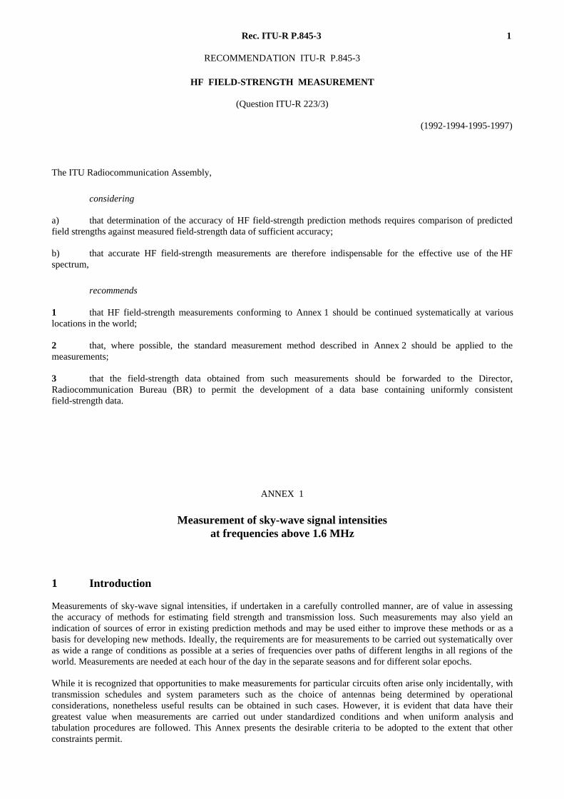
Signal-intensity data are required from circuits of different ranges in all geographical regions. Recordings of a giventransmission should be made for as many hours as possible every day. The objective should be to derive the median andother percentile values of the day-to-day distribution of signal intensity over all days of the month. Where it is notfeasible to carry out measurements every day, uncertainties arise in estimates of these values. Assuming a log-normallaw of variation with decile deviation from the median of D (dB), the standard error E in the median based on a sampleof N days within a month of 30 days (see Fig. 1) is:

E = D

1.28 1N –

130 dB (1)

0845-01

15

10

5

010 20 301

D = 20 dB1510

5

E (

dB)

FIGURE 1

Standard error in monthly median (E)as a function of number of days sampled (N) for different

decile deviations from the median (D)

N

FIGURE 1/PI.845-1 [D01] = 10 cm

Clearly the standard error increases as the number of days of recording decreases. While there is no limiting sample sizegiving an abrupt increase in error, as a general rule 10 or more measurements are required for the calculation of themedians, 14 for the quartiles and 18 for the deciles.

It is seldom feasible to embark on a measurement programme extending over a significant part of a solar cycle but toease data interpretation and to be statistically meaningful, measurements should cover a minimum period of one year at agiven fixed frequency. There are particular advantages in attempting to record signals simultaneously over a path at aseries of different frequencies, both to aid the understanding of propagation effects and to permit quantitative data to beobtained by night when maximum usable frequencies are low, as well as by day when there is much absorption at thelower frequencies so that signals are masked by background noise.

3 Transmitter and transmitting antenna

The transmitter should be unambiguously identifiable so as to be sure that what is recorded is the wanted transmissionand not co-channel signals, adjacent channel signals, or interfering noise. It is useful if the signals are interrupted atsome periodic rate, say for 5 min once every hour, both as an aid to transmitter identification and to determine receivedbackground levels as confirmation that there is no significant signal contamination. The transmitter should operate

Rec. ITU-R P.845-3 3

preferably for 24 h per day. It must be stable in both frequency and radiated power, and these two parameters must beknown accurately. For reception over short paths it should desirably have a radiated power in excess of 1 kW and overmedium distance and long paths a power of 10 kW or more. Where a special transmitter is operated, this would normallyradiate continuous waves, although other waveforms may be used to study the characteristics of individual propagationmodes. If use is made of commercial transmitters carrying modulated signals, it is important that the type of modulationshould be constant and the mean percentage modulation should not vary. Narrow-band transmissions (approximately1 kHz bandwidth or less) or a narrow-band component of a composite signal are most appropriate to record. Widerbandwidth signals are liable to interference contamination. Standard-frequency transmissions have been employed in thepast, but in many receiver locations there is now serious interference between signals from different transmittersoperating this service and sharing the same frequency. Nevertheless, interference can be avoided to some extent bymeans of a narrow-band receiver capable of resolving the different audio modulation frequencies of each co-channeltransmitter. Transmitters for point-to-point telephony or telegraphy services offer the advantages of providing channelswhich are relatively free from interference, and a detailed log of transmission schedules is usually available. On the otherhand, these transmitters often employ high-gain antennas, which tends to be a disadvantage.

A suitable category of transmitters meeting nearly all of the above criteria is weather-chart (FAX) transmitters usingfrequency shift-keying (± 400 Hz). As there are numbers of receivers (ships) with unknown position, these transmittersuse omnidirectional antennas and transmit mostly for 24 h per day. Receiving systems should be very sensitiveespecially when recordings are made for very long paths.

Inspection of the International Frequency List maintained by the BR is of value in the selection of suitable transmitters tomonitor. In particular, this usually gives information concerning transmitter radiated power, form of modulation andperiod of the day of operation. Sometimes it also yields details of the antenna type and orientation. The InternationalFrequency List is useful additionally in providing a list of co-channel and adjacent-channel transmitters which should beconsidered further to assess the likelihood of possible interference. However, before embarking on a programme ofsystematic measurements it is recommended that after selecting a potentially suitable transmitter in this way, firstly aseries of monitoring measurements should be carried out at various times over a period of about a month to determinethe order of signal intensities encountered, the time coverage over which such signals can be detected, and the amountsof interference experienced. Then, a direct approach should be made to the organization operating the transmitter toverify the International Frequency List entries, to supply such additional details as are required – for example,concerning the type of antenna used and the associated ground properties. In particular, it should be checked that theradiated power is maintained constant, that different antennas are not used by night and day, and that the transmitter isnot part of a network of transmitters operating at the same frequency from geographically separated sites – a procedureadopted in the HF broadcasting services in some countries. It is important to confirm also that it is proposed that thetransmitter will remain operational throughout the whole period for which it is intended to make measurements. Onlythen should a decision be reached to carry out systematic recordings of the transmissions. Whilst ideally it would bedesirable to receive details of the transmitter log, noting in particular any malfunctions or temporary changes in technicalcharacteristics which might influence the measurements, it is rarely feasible to obtain such data and to apply variablecorrections to results in retrospect. Instead, every effort should be taken at the outset to avoid the monitoring oftransmitters whose characteristics are known to fluctuate.

For a particular transmitter to be suitable for signal-intensity measurements, the performance of its transmitting antennaneeds to be known accurately. Transmitters coupled to antennas with little directivity have advantages over those withhighly-directional antennas because radiation patterns usually approximate more closely to theory, because the relativestrengths at the receiving site of signals travelling via different modes are then determined mainly by propagationeffects, and because valid deductions may be made with a single allowance for transmitting-antenna gain in the absenceof a knowledge of wave launch directions. Unfortunately though, low-gain transmitting antennas are seldom used forother applications. Most point-to-point HF land-fixed communication circuits employ high-gain rhombic or log-periodicantennas; for sky-wave broadcasting, arrays of horizontal dipoles, also with significant directivity, are popular. Theexception is with standard-time transmitters which aim to provide all-round azimuthal coverage by means of verticalhalf-wavelength dipoles. These transmissions are particularly suitable for monitoring purposes. Radiation patterns for avertical-dipole antenna may be estimated fairly accurately, except at low elevation angles where the particular groundconstants control signal intensities. However, even at low angles the performance is known more accurately than formost other types of antenna. If no such transmitter is conveniently positioned for use, then before monitoringtransmissions from a directional antenna it should be checked that the great-circle path to the receiver does not involve

4 Rec. ITU-R P.845-3

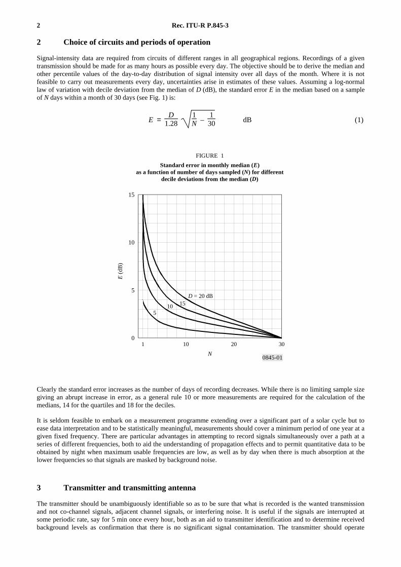
reception of side-lobe signals. If propagation is over medium or long distances, ideally the antenna vertical polardiagram for elevation angles less than 20° should approximate that of a reference short vertical radiator sited overaverage ground (see Fig. 2a)).

Where a special transmitter is operated, a short vertical antenna is to be preferred. Alternatively, for short paths ahorizontal dipole aligned for broadside radiation along the great-circle direction may be used. For greater rangescorresponding to low elevation angles, the direct and ground-reflected components of the sky wave nearly cancel oneanother so that a horizontal antenna is very inefficient unless elevated to a great height and should be avoided.

Transmitting-antenna gain (like receiving-antenna gain) is best determined from near-site measurements in the far-fieldregion, but it is recognized that these rarely form part of the normal programme of work at a transmitting installation andthat it is not generally possible to be able to arrange for such measurements to be carried out at a remote location, notunder the control of the receiving organization. Accordingly, transmitting-antenna gain must usually be calculated fromtheoretical relationships in terms of the known antenna geometry, and by making certain assumptions concerning thetype of ground involved.

4 Receiving antenna, receiver and recording techniques

Since existing methods of prediction of signal intensities do not take account of field distortion effects due to localfeatures at the receiving site such as undulating ground, obstacles like buildings and foliage and adjacent antennas whichact as re-radiating structures, it is important to site the receiving antenna so that these effects are kept to a minimum. Theground should have a slope not exceeding 2° out to a distance of five wavelengths and no obstacles should subtend anangle from the horizontal at the centre of the antenna in excess of 5°. The separation from other antennas should be notless than ten times the antenna length.

It is more important that the receiving-antenna performance should be known accurately than that it should have highgain. Except at the lower frequencies during the daytime when there is much ionospheric absorption, threshold levels forsignal detection will normally be determined by external noise intensities whatever receiving antenna is used. In general,the greater the antenna gain, the more likely the possibility of error in assessing its performance. Accordingly, a shortvertical active antenna or a grounded vertical monopole antenna not exceeding a quarter wavelength high or a small loopantenna are most appropriate to employ. The loop antenna would normally be aligned in a vertical plane containing thegreat-circle direction to the transmitter. For long-distance paths where off-great circle propagation is likely to beimportant, the vertical-monopole antenna is preferable since this provides omnidirectional azimuthal pick-up. If severaltransmissions from different azimuths are recorded with one antenna, only a vertical antenna should be used. Someorganizations use vertical monopoles for signal measurements but standardize results by means of calibration datainvolving comparisons for selected sample signals with the pick-up indicated by a portable “field-strength” meterincorporating an integral loop-receiving antenna.

Figure 2a) shows the variation with elevation angle of the term E0 – E (a measure of the signal pick-up resulting from adowncoming sky-wave of constant intensity and its associated ground-reflected wave, defined in § 6.2) for a shortvertical grounded monopole and a loop antenna, both situated over average ground. For elevation angles belowabout 30° the monopole and loop antennas have very similar polar diagrams but at higher elevation angles theloop-antenna pattern is preferable since the pick-up is relatively insensitive to angle. Figure 2b) shows the effect ofantenna siting over ground of different properties. Signal pick-up for wet ground exceeds that for very dry ground bysome 2-6 dB with the largest differences occurring at low elevation angles. The marked dependence of the pick-up onthe ground constants and on the elevation angle when this is low, which has been discussed already with regard to thetransmitting antenna, leads to particular data interpretation difficulties for long paths where elevation angles are notknown accurately. In principle, the use of an artificial ground screen would lead to a receiving system performance lessdependent on weather conditions which affect ground water content. The screen would improve the ground constantsand so increase the signal pick-up, but to be effective in this role it would need to have dimensions of the order of tens ofwavelengths and this is rarely practicable. On the other hand, short screens of length up to about five wavelengths can beimplemented and are of value in stabilizing antenna impedances to improve circuit matching. If a screen is used, it isdesirable to assess its effect by carrying out near-site calibration measurements with signals radiated in the far-fieldregion from an airborne transmitter.

Rec. ITU-R P.845-3 5

0845-02

– 15

– 10

– 5

0

5

0 10 20 30 40 50 60

E

– E

(d

B)

0E

–

E

(dB

)0

A

B

C

– 15

– 10

– 5

0

5

0 10 20 30 40 50 60

Elevation angle (degrees)

a) Monopole and loop sited over average ground of conductivity σ = 0.01 S/m, relative dielectric constant ε = 15

monopole

loop

Elevation angle (degrees)

b) Loop sited over wet, average and very dry ground

Curves A: wet ground σ = 0.02 S/m, ε = 20 B: average ground σ = 0.01 S/m, ε = 15 C: very dry ground σ = 0.002 S/m, ε = 5

FIGURE 2

Difference between r.m.s. equivalent-incident field strength, E0, and r.m.s.sky-wave field strength, E, for short vertical monopole

and for loop antenna at a height of 1 m. Frequency: 15 MHz

FIGURE 2/PI.845...[D02] = 23.5 CM PAGE PLEINE

Horizontal half-wave dipoles for single-frequency operation or terminated dipoles for multiple-frequency measurementsare sometimes suitable for reception of signals on short paths. In particular, pick-up is not strongly dependent on theground constants. However, for medium distance and long paths when elevation angles are low, these antennas provide

6 Rec. ITU-R P.845-3

only limited pick-up, again markedly dependent on elevation angle, unless they are elevated to great heights. Theyshould not be used for these paths because of calibration difficulties.

Some organizations are equipped to make measurements using special antenna systems, such as rhombic arrays,designed for specific circuits to improve signal/noise ratios and to enable measurements to be made under conditionswhere a simple antenna would be unusable. It is difficult to interpret the results obtained on an extended antenna systemin the presence of a complex field built up of several waves incident at different angles, but measurements made withsuch antennas may be acceptable for the purpose in hand, if they can be related consistently to those that would beobtained at the same time on a standard antenna. In making a choice between antennas responding either to vertical orhorizontal polarization, it is prudent to check that, if propagation paths involve waves with markedly non-circularpolarization, reception (or transmission) is predominantly that of the stronger ordinary wave.

The receiving antenna should be connected to the receiver via a buried coaxial cable and appropriate matching circuitry.This latter may take the form of a transformer or a wideband pre-amplifier. The receiver bandwidth should be as narrowas possible consistent with the bandwidth of the transmitted signals, in order to optimize the received signal/noise ratio.For continuous-wave signals and for the monitoring of the steady tone sideband signals of standard-time transmissions,bandwidths of the order of 100 Hz or less are suggested.

Received signal intensity depends on radiated power within the receiver bandwidth. This is a function of the carrier,modulation and recording arrangement. For a receiver bandwidth which encompasses the carrier and all sidebands, theoperative radiated power is equal to the sum of that of the carrier and all other components. Figures for different types ofmodulation are given in Recommendation ITU-R SM.326. In the case of narrowband reception of a single sideband of astandard time transmission of carrier power P where the amplitude modulation depth is m, the sideband power is m2P/4.

Signals should be detected, applied to appropriate integration-smoothing circuitry, and then recorded in suitable form.

Some organizations monitor signals over oblique paths in order to note the occurrence of events like sudden ionosphericdisturbances (SIDs) and magnetic storms, or to study fading statistics. In these cases, special recording procedures maybe necessary. Where, however, the prime requirements are to collect representative hourly signal-intensity data,measurements are best made using a pen-chart recorder with a logarithmic amplitude scale (i.e. linear in decibels) and achart speed of about 2 cm per hour. The integration time constant should be about 20 s. This arrangement provides aconvenient length of record for manual smoothing whilst at the same time permitting the rejection of sections shown tobe contaminated by interfering signals or strong atmospherics. It is often simpler to record the automatic gain-controlvoltage from a commercial receiver after modifications to equate and lengthen the rise and decay time constants to the20 s noted above. However, this approach may lead to unacceptable errors under some conditions, even aftercontinuous-wave calibration of the response. Output voltage is usually approximately proportional to the logarithm ofthe input voltage, but since this non-linearity is associated with the detection process and occurs prior to integration,recordings give the mean logarithm of the signal intensity and not the mean in logarithmic units as required. Thesequantities differ when there is signal fading present. An alternative acceptable form of recording involves digitalquantization of instantaneous amplitudes at a convenient sampling rate so as to cover the known periodicity of typicalfading components (with fading durations up to about 20 min). Representative values may then be determined bycomputer processing. Apart from identification problems, the use of a computer to control the measuring receiver cangreatly accelerate and simplify both measurements and statistical analysis. It cannot be emphasized too strongly thoughthat with these techniques some form of regular check must be introduced to ensure that what is measured is the wantedtransmission.

Hourly figures each day are best expressed in the form of median values. With chart recording it is preferable to derivethe median directly as that amplitude which is exceeded for a total of half the recording duration (i.e. 30 min for hourlymedians). This procedure is independent of the chart amplitude scale. When a precise logarithmic amplitude scale isused for recording, the median may alternatively be given approximately by two-thirds the chart deflection between thequasi-minimum value (exceeded for Q% of the time, say, where Q ≥ 90%) and the quasi-maximum value (exceeded for(100 – Q)% of the time), assuming that fading follows a Rayleigh distribution. With computer recording and processingit is suggested in Annex 2 that a minimum of 12 independent samples are needed to produce representative hourlymedian values. The samples should ideally be distributed uniformly throughout the hour, but if switched recording ofsignals from several transmitters is required, groups of 4 samples within 4 min, repeated three times during the hour, areacceptable.

Rec. ITU-R P.845-3 7

5 Calibration measurements

Pen-chart recorder deflections or computer-recorded data should be related to the associated voltages injected directlyinto the receiver from a signal generator. Periodic calibration measurements are needed to express r.m.s. signal-generatorvoltage readings in terms of the corresponding amplitudes of the recorded sky waves. Two approaches are possible. Inthe one, cable, mis-match and coupling losses, together with antenna impedance measurements, are needed so that signaldata may be expressed as available receiver powers and associated field strengths. In the other, appropriate only toreception of vertically-polarized wave components, a direct comparison is made with meter values indicated by aportable “field-strength” measuring system incorporating a vertical loop antenna. In this case, it is important to be certainwhat assumptions have been made in calibrating the meter and what field strengths are quoted (see § 6.2).

6 Conversion of measured data to mean available receiver power and r.m.s. sky-wavefield strength

The existing method of Recommendation ITU-R P.533 for estimating sky-wave signal intensities gives values of meanavailable receiver power in the absence of receiving-system losses and r.m.s. sky-wave field strength. Hence, conversionrelationships are needed between the measured voltages developed across the receiver input terminals and thesequantities.

6.1 Mean available receiver power

The relationship between measured receiver input voltage when fed from a practical antenna and the available powerfrom an idealized lossless receiving antenna coupled to a matched load depends on the receiving-system losses and theimpedances of the antenna and receiver. In general, the receiving-system losses and the antenna impedance arefrequency-dependent factors. In particular, the relationship is not a function of the wave-arrival directions orpolarizations.

Consider first the idealized case of a lossless receiving antenna feeding a matched load.

Let

Pa : available power from receiving antenna (dBW)

V0 : r.m.s. voltage developed across matched load (dB(1 µV))

r : antenna load resistance (Ω).

Then

Pa = V0 – 10 log r – 120

In particular for r = 50 Ω:

Pa = V0 – 137 dB (2)

Now consider the practical case of an antenna coupled to a receiver via a feeder cable and a transformer or othermatching circuitry, but where some matching losses arise, r is then the load resistance presented by the receiver.

Let

Vr : r.m.s. voltage developed across receiver input terminals (dB(1 µV))

L : cable loss (dB)

T : mis-match and coupling losses (dB).

In general, the evaluation of T involves a knowledge of the antenna impedance. T includes losses in transformers andother antenna-matching circuitry, and losses associated with the matching of the feeder cable to the receiver. Then

V0 = Vr + L + T

so that, from equation (2):

Pa = Vr + L + T – 137 dB (3)

8 Rec. ITU-R P.845-3

Now for reception of fading sky-wave signals where Pa represents the mean available power (dBW) and Vm is thehourly median receiver input voltage (dB(1 µV)), a fading allowance must be included in equation (3). AssumingRayleigh fading, the r.m.s. voltage is 1.6 dB greater than the median, so that:

Pa = Vm + L + T – 135.4 dB (4)

Equation (4) may be used to relate measured values of Vm to Pa provided the various system losses are known. If it is notpossible to determine L and T as, for example, where calibration is by standardization with a portable field-strengthmeter, then alternatively Pa may be given in terms of E, the r.m.s. sky-wave field strength (dB(µV/m)), when this isknown (see § 6.2), by

Pa = E + Gr – 120 + 10 log

λ2

480 π2

= E + Gr – 20 log ƒ – 107.2 dB(5)

λ is the wavelength (m) and f the frequency (MHz). Gr is the receiving antenna gain (expressed in decibels relative to anisotropic radiator in free space) which, in particular, depends on wave-arrival direction. This direction is not usuallymeasured but must be predicted. Hence, this means of deriving Pa is less appropriate, since it does not lead toindependent data to test the accuracy of the predictions.

6.2 R.m.s. sky-wave field strength

Measured receiver input voltages may be expressed in terms of the corresponding voltages induced in the receivingantenna, and thence as associated field strengths. In the case of simple configurations such as a vertical monopoleantenna and a broadside or end-on dipole or loop antenna responding to waves with a single (horizontal or vertical)polarization, it is convenient to introduce the concept of an equivalent-incident field strength. This refers to a resultantfield with the same polarization as that to which the antenna responds. It may be regarded as the sum of a downcomingsky wave and a ground-reflected wave. Portable commercial field-strength meters are usually calibrated to indicateequivalent-incident field strength. On the other hand, for extended antennas composed of separate limbs with differentorientations, such as the horizontal rhombic antenna, the term “equivalent-incident field strength” has no physicalsignificance. The signal pick-up and the resultant field vary for the different limbs. In the case of the off-axis pick-up ona simple antenna like a dipole or a loop antenna, the equivalent-incident field concept also is not particularly useful. Theantenna then responds to waves of elliptical polarization, and induced voltages depend not only on the wave strengths,but also on the match between the wave polarizations and the polarizations to which the antenna responds for theparticular directions of incidence. Waves of different polarization and intensity incident from the same direction maythen produce the same induced voltage.

The relationship between equivalent-incident field strength and voltage induced in the receiving antenna is a function offrequency, but unlike the corresponding relationship for sky-wave field strength, it is independent of wave-arrivaldirection and ground constants. In both cases the conversion factor has the dimensions of length, so that where theconcept of an equivalent-incident field strength is meaningful, it is convenient to refer to two different antenna effectivelengths. Let lei be the effective length relating equivalent-incident field strength to antenna induced e.m.f., and les be theeffective length relating sky-wave field strength to antenna induced e.m.f. To compare equivalent-incident field strengthand sky-wave field strength, which is the same as to relate lei to an appropriate les, is usually complicated and involvesassumptions about the prevailing wave-field component amplitudes, polarizations and arrival angles; also a knowledgeof the antenna polar diagram is required.

Let

E0 : r.m.s. equivalent-incident field strength (dB(µV/m))

Vm : median voltage developed across receiver input terminals (dB(1 µV))

Rec. ITU-R P.845-3 9

and let lei be expressed in metres. Then again assuming Rayleigh fading:

E0 = Vm + L + T – 20 log (lei) + 7.6 dB (6)

For a vertical monopole of physical length l (m)

lei = λ2π tan

π lλ (7)

and in particular for l << λ, lei ∼– l2.

For a small n-turn loop antenna of area A aligned in the plane of incidence:

lei = 2π n A

λ (8)

Now if E is the r.m.s. sky-wave field strength (dB(µV/m)), and les is expressed in metres, then comparison withequation (6) leads to:

E = Vm + L + T – 20 log (les) + 7.6 dB (9)

But les is given in terms of the antenna gain relative to an isotropic antenna in free space gr and radiation resistancera (Ω) by:

l 2es =

gr λ2 ra 120 π2 (10)

so that with Gr = 10 log gr and f (MHz), E may be expressed alternatively as:

E = Vm + L + T – Gr – 10 log ra + 20 log ƒ – 11.2 dB (11)

The difference between equivalent-incident field strength and sky-wave field strength is given from equations (6) to (11)by equating values of Vm. This is shown in Fig. 2 for the cases of a short vertical grounded monopole and a loopantenna.

6.3 Preferred signal-intensity parameter for comparison of measured data with predictions

It has been seen in § 6.1 and 6.2 that whereas measured data are related to available receiver power in terms of thereceiving-system parameters only, to express the measurements as corresponding sky-wave field strengths involves aknowledge of wave-arrival directions and polarizations. Since these directions are not normally measured but must bepredicted, it follows that, where possible, the preferred signal-intensity parameter for the purpose of comparisonexercises with predictions is the available receiver power. Therefore, it is recommended that when a new HF fieldstrength measurement is made, the available receiver power Pa is derived directly from measured values of Vm by theuse of equation (4) in § 6.1. On the other hand, in order to derive Pa from the monthly median value of the r.m.s. fieldstrength E in the Data Bank D1, the following equation derived from both equations (4) and (11) should be applied:

Pa = E + Gr + 10 log ra – 20 log f – 124.2 dBW (12)

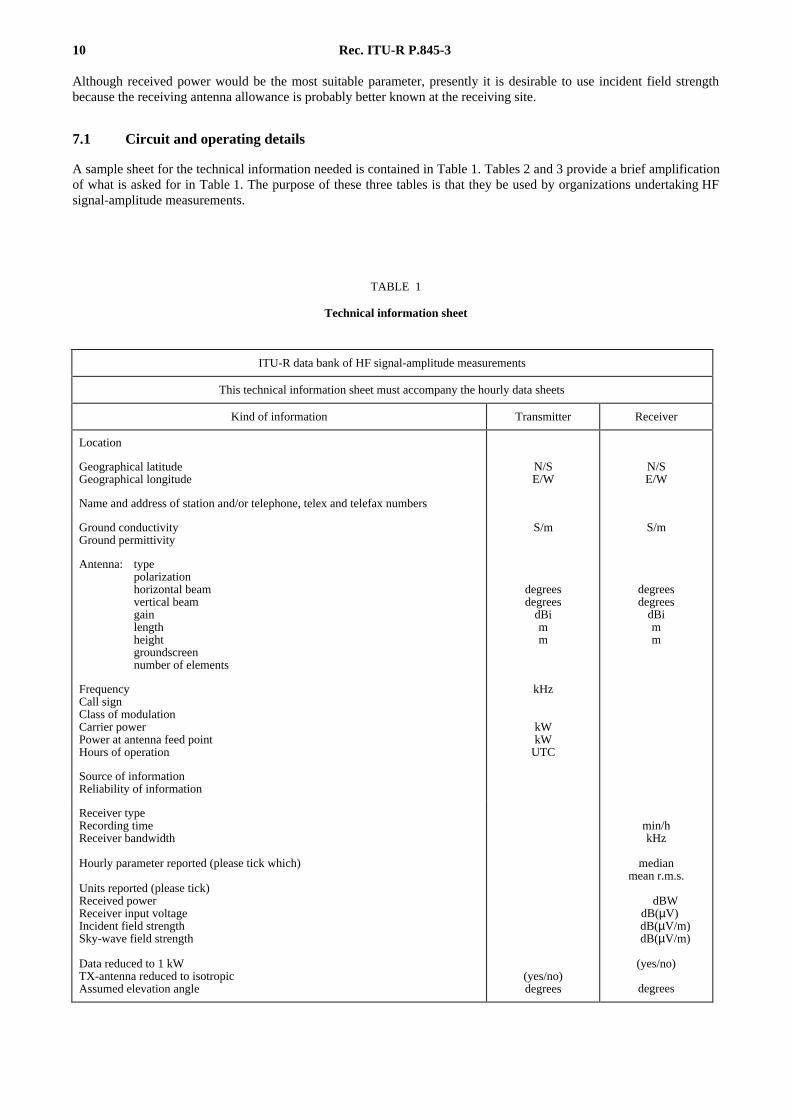
7 Data-tabulation procedures

Four types of data-tabulation sheet may be prepared, depending on whether it is the wish of the organization undertakingmeasurements to quote values in:

– received power (dBW) (without correcting for receiving antenna effects);

– receiver input voltage (dB(µV)) (without correcting for receiving antenna effects);

– incident field strength (dB(µV/m)) (receiving antenna allowance ignores reflection of the downcoming sky-wavenear the receiving antenna);

– sky-wave field strength (dB(µV/m)).

10 Rec. ITU-R P.845-3

Although received power would be the most suitable parameter, presently it is desirable to use incident field strengthbecause the receiving antenna allowance is probably better known at the receiving site.

7.1 Circuit and operating details

A sample sheet for the technical information needed is contained in Table 1. Tables 2 and 3 provide a brief amplificationof what is asked for in Table 1. The purpose of these three tables is that they be used by organizations undertaking HFsignal-amplitude measurements.

TABLE 1

Technical information sheet

ITU-R data bank of HF signal-amplitude measurements

This technical information sheet must accompany the hourly data sheets

Kind of information Transmitter Receiver

Location

Geographical latitudeGeographical longitude

Name and address of station and/or telephone, telex and telefax numbers

Ground conductivityGround permittivity

Antenna: typepolarizationhorizontal beamvertical beamgainlengthheightgroundscreennumber of elements

N/SE/W

S/m

degreesdegrees

dBimm

N/SE/W

S/m

degreesdegrees

dBimm

FrequencyCall signClass of modulationCarrier powerPower at antenna feed pointHours of operation

Source of informationReliability of information

kHz

kWkW

UTC

Receiver typeRecording timeReceiver bandwidth

Hourly parameter reported (please tick which)

Units reported (please tick)Received powerReceiver input voltageIncident field strengthSky-wave field strength

Data reduced to 1 kWTX-antenna reduced to isotropicAssumed elevation angle

(yes/no)degrees

min/hkHz

medianmean r.m.s.

dBWdB(µV)dB(µV/m)dB(µV/m)

(yes/no)

degrees

Rec. ITU-R P.845-3 11

7.2 Monthly tabulation sheets of signal-amplitude measurements

Table 4 contains a sample sheet for recording the hourly and monthly values of signal-amplitude measurements. Table 5explains Table 4. Table 4 is required for each frequency and month, whereas Table 1 is only needed once for eachfrequency.

The evaluation of count, upper and lower deciles, upper and lower quartiles and median is done by a computer or, if notavailable, by means of the procedure described in Table 6.

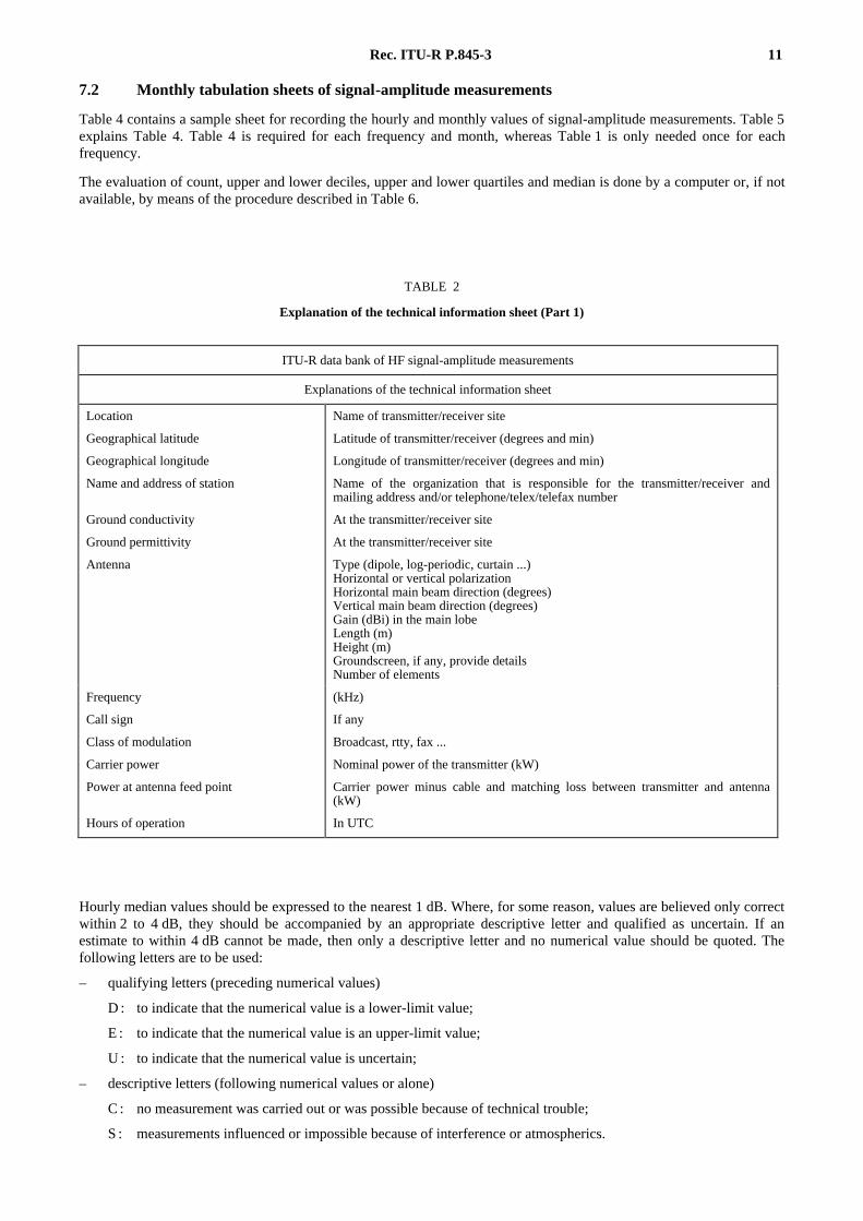
TABLE 2

Explanation of the technical information sheet (Part 1)

Hourly median values should be expressed to the nearest 1 dB. Where, for some reason, values are believed only correctwithin 2 to 4 dB, they should be accompanied by an appropriate descriptive letter and qualified as uncertain. If anestimate to within 4 dB cannot be made, then only a descriptive letter and no numerical value should be quoted. Thefollowing letters are to be used:

– qualifying letters (preceding numerical values)

D : to indicate that the numerical value is a lower-limit value;

E : to indicate that the numerical value is an upper-limit value;

U : to indicate that the numerical value is uncertain;

– descriptive letters (following numerical values or alone)

C : no measurement was carried out or was possible because of technical trouble;

S : measurements influenced or impossible because of interference or atmospherics.

ITU-R data bank of HF signal-amplitude measurements

Explanations of the technical information sheet

Location

Geographical latitude

Geographical longitude

Name and address of station

Ground conductivity

Ground permittivity

Antenna

Name of transmitter/receiver site

Latitude of transmitter/receiver (degrees and min)

Longitude of transmitter/receiver (degrees and min)

Name of the organization that is responsible for the transmitter/receiver andmailing address and/or telephone/telex/telefax number

At the transmitter/receiver site

At the transmitter/receiver site

Type (dipole, log-periodic, curtain ...)Horizontal or vertical polarizationHorizontal main beam direction (degrees)Vertical main beam direction (degrees)Gain (dBi) in the main lobeLength (m)Height (m)Groundscreen, if any, provide detailsNumber of elements

Frequency

Call sign

Class of modulation

Carrier power

Power at antenna feed point

Hours of operation

(kHz)

If any

Broadcast, rtty, fax ...

Nominal power of the transmitter (kW)

Carrier power minus cable and matching loss between transmitter and antenna(kW)

In UTC

12 Rec. ITU-R P.845-3

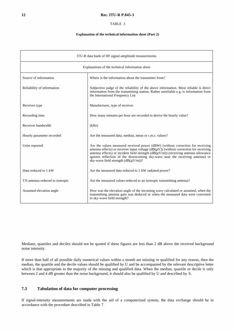
TABLE 3

Explanation of the technical information sheet (Part 2)

Medians, quartiles and deciles should not be quoted if these figures are less than 2 dB above the received backgroundnoise intensity.

If more than half of all possible daily numerical values within a month are missing or qualified for any reason, then themedian, the quartile and the decile values should be qualified by U and be accompanied by the relevant descriptive letterwhich is that appropriate to the majority of the missing and qualified data. When the median, quartile or decile is onlybetween 2 and 4 dB greater than the noise background, it should also be qualified by U and described by S.

7.3 Tabulation of data for computer processing

If signal-intensity measurements are made with the aid of a computerized system, the data exchange should be inaccordance with the procedure described in Table 7.

ITU-R data bank of HF signal-amplitude measurements

Explanations of the technical information sheet

Source of information Where is the information about the transmitter from?

Reliability of information Subjective judge of the reliability of the above information. Most reliable is directinformation from the transmitting station. Rather unreliable e.g. is information fromthe International Frequency List

Receiver type Manufacturer, type of receiver

Recording time How many minutes per hour are recorded to derive the hourly value?

Receiver bandwidth (kHz)

Hourly parameter recorded Are the measured data, median, mean or r.m.s. values?

Units reported Are the values measured received power (dBW) (without correction for receivingantenna effects) or receiver input voltage (dB(µV)) (without correction for receivingantenna effects) or incident field strength (dB(µV/m)) (receiving antenna allowanceignores reflection of the downcoming sky-wave near the receiving antenna) orsky-wave field strength (dB(µV/m))?

Data reduced to 1 kW Are the measured data reduced to 1 kW radiated power?

TX-antenna reduced to isotropic Are the measured values reduced to an isotropic transmitting antenna?

Assumed elevation angle How was the elevation angle of the incoming wave calculated or assumed, when thetransmitting antenna gain was deduced or when the measured data were convertedto sky-wave field strength?

Rec. IT

U-R

P.845-3

13

0030-0130

0230-0330

0330-0430

0430-0530

0530-0630

0630-0730

0730-0830

0830-0930

0930-1030

1030-1130

1130-1230

1230-1330

1330-1430

1430-1530

1530-1630

1630-1730

1730-1830

1830-1930

1930-2030

2030-2130

2130-2230

2230-2330

2330-0030

0130-0230

1234

5678

9101112

13141516

17181920

21222324

25262728

293031CountUpper decileUpper quartileMedian

Lower quartileLower decile

Day

TABLE 4

Sample sheet for hourly and monthly signal-amplitude measurements

Time UTC

ITU-R data bank of HF signal-amplitude measurements Circuit: Frequency: kHz Month: Year:

Qualifying letters:Descriptive letters:

D: S:

U: uncertain valueE: C:

receiver input below recording thresholdno measurement carried out or technical trouble

receiver input above recording maximuminterference

14 Rec. ITU-R P.845-3

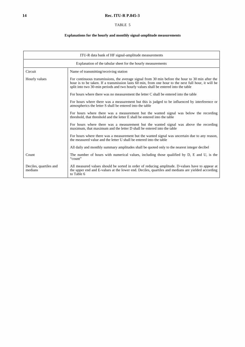
TABLE 5

Explanations for the hourly and monthly signal-amplitude measurements

ITU-R data bank of HF signal-amplitude measurements

Explanation of the tabular sheet for the hourly measurements

Circuit Name of transmitting/receiving station

Hourly values For continuous transmissions, the average signal from 30 min before the hour to 30 min after thehour is to be taken. If a transmission lasts 60 min, from one hour to the next full hour, it will besplit into two 30-min periods and two hourly values shall be entered into the table

For hours where there was no measurement the letter C shall be entered into the table

For hours where there was a measurement but this is judged to be influenced by interference oratmospherics the letter S shall be entered into the table

For hours where there was a measurement but the wanted signal was below the recordingthreshold, that threshold and the letter E shall be entered into the table

For hours where there was a measurement but the wanted signal was above the recordingmaximum, that maximum and the letter D shall be entered into the table

For hours where there was a measurement but the wanted signal was uncertain due to any reason,the measured value and the letter U shall be entered into the table

All daily and monthly summary amplitudes shall be quoted only to the nearest integer decibel

Count The number of hours with numerical values, including those qualified by D, E and U, is the“count”

Deciles, quartiles andmedians

All measured values should be sorted in order of reducing amplitude. D-values have to appear atthe upper end and E-values at the lower end. Deciles, quartiles and medians are yielded accordingto Table 6

Rec. ITU-R P.845-3 15

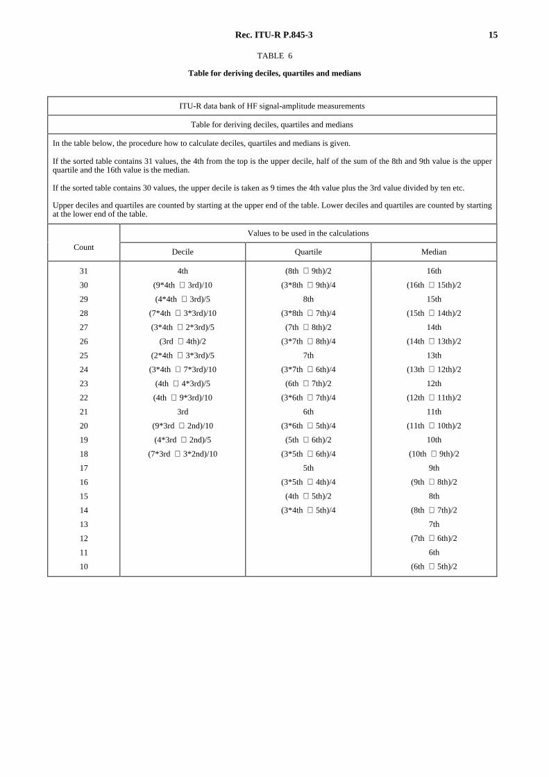
TABLE 6

Table for deriving deciles, quartiles and medians

ITU-R data bank of HF signal-amplitude measurements

Table for deriving deciles, quartiles and medians

In the table below, the procedure how to calculate deciles, quartiles and medians is given.

If the sorted table contains 31 values, the 4th from the top is the upper decile, half of the sum of the 8th and 9th value is the upperquartile and the 16th value is the median.

If the sorted table contains 30 values, the upper decile is taken as 9 times the 4th value plus the 3rd value divided by ten etc.

Upper deciles and quartiles are counted by starting at the upper end of the table. Lower deciles and quartiles are counted by startingat the lower end of the table.

Values to be used in the calculations

Count Decile Quartile Median

31

30

29

28

27

26

25

24

23

22

21

20

19

18

17

16

15

14

13

12

11

10

4th

(9*4th + 3rd)/10

(4*4th + 3rd)/5

(7*4th + 3*3rd)/10

(3*4th + 2*3rd)/5

(3rd + 4th)/2

(2*4th + 3*3rd)/5

(3*4th + 7*3rd)/10

(4th + 4*3rd)/5

(4th + 9*3rd)/10

3rd

(9*3rd + 2nd)/10

(4*3rd + 2nd)/5

(7*3rd + 3*2nd)/10

(8th + 9th)/2

(3*8th + 9th)/4

8th

(3*8th + 7th)/4

(7th + 8th)/2

(3*7th + 8th)/4

7th

(3*7th + 6th)/4

(6th + 7th)/2

(3*6th + 7th)/4

6th

(3*6th + 5th)/4

(5th + 6th)/2

(3*5th + 6th)/4

5th

(3*5th + 4th)/4

(4th + 5th)/2

(3*4th + 5th)/4

16th

(16th + 15th)/2

15th

(15th + 14th)/2

14th

(14th + 13th)/2

13th

(13th + 12th)/2

12th

(12th + 11th)/2

11th

(11th + 10th)/2

10th

(10th + 9th)/2

9th

(9th + 8th)/2

8th

(8th + 7th)/2

7th

(7th + 6th)/2

6th

(6th + 5th)/2

16 Rec. ITU-R P.845-3

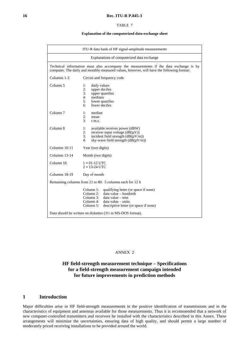
TABLE 7

Explanation of the computerized data-exchange sheet

ANNEX 2

HF field-strength measurement technique – Specificationsfor a field-strength measurement campaign intended

for future improvements in prediction methods

1 Introduction

Major difficulties arise in HF field-strength measurements in the positive identification of transmissions and in thecharacteristics of equipment and antennas available for those measurements. Thus it is recommended that a network ofnew computer-controlled transmitters and receivers be installed with the characteristics described in this Annex. Thesearrangements will minimize the uncertainties, ensuring data of high quality, and should permit a large number ofmoderately priced receiving installations to be provided around the world.

ITU-R data bank of HF signal-amplitude measurements

Explanations of computerized data exchange

Technical information must also accompany the measurements if the data exchange is bycomputer. The daily and monthly measured values, however, will have the following format:

Columns 1-3 Circuit and frequency code

Column 5 1: daily values2: upper deciles3: upper quartiles4: medians5: lower quartiles6: lower deciles

Column 7 1: median2: mean3: r.m.s.

Column 8 1: available receiver power (dBW)2: receiver input voltage (dB(µV))3: incident field strength (dB(µV/m))4: sky-wave field strength (dB(µV/m))

Columns 10-11 Year (two digits)

Columns 13-14 Month (two digits)

Column 16 1 = 01-12 UTC2 = 13-24 UTC

Columns 18-19 Day of month

Remaining columns from 21 to 80: 5 columns each for 12 h

Column 1: qualifying letter (or space if none)Column 2: data value – hundredsColumn 3: data value – tensColumn 4: data value – unitsColumn 5: descriptive letter (or space if none)

Data should be written on diskettes (3½ in MS-DOS format).

Rec. ITU-R P.845-3 17

2 The HF field-strength measurement campaign

The required data cannot be obtained unless new transmitters and receivers are installed. It is recommended that thesetransmitters should be frequency agile, each radiating on up to five frequencies sequentially according to apredetermined schedule. In each case there should be a period of steady signal emission for manual measurements andcoded sequences permitting aural identification of the source, computer identification of the source and computerevaluation of the intensities of both the signal and the background noise or interference.

To minimize the possibility of interference, the transmissions should be on assigned frequencies probably in the fixedservice bands.

A number of receiver implementations are possible, meeting the specification given below, but a single standard for thereceiving antenna is recommended. Each receiver should operate on a rapid measuring sequence, dwelling on eachfrequency for up to 12 s, and should be able to measure signal levels on many of the transmitted frequencies during eachhour. At least one model of receiver, including the interface, computer and software, is available and it is hoped thatsome administrations will provide some equipments on loan to those developing countries where there is a great need fornew measurement data.

3 Transmitter

3.1 Transmitter locations

In order to collect data representative of HF propagation conditions on a worldwide scale, there should preferably be atleast nine transmitters. These should be located in the Northern and Southern Hemispheres at middle latitudes and in thetropics in Regions 1, 2 and 3 (see Table 8). It should be noted however that useful results can be obtained from a morelimited number of transmitters should the distribution proposed in Table 8 not become available.

TABLE 8

3.2 Transmitter power

Transmitter power should be in the range of 5-10 kW.

3.3 Transmitting antennas

Transmitting antennas should be omnidirectional in azimuth and should have a broad elevation pattern. In order to avoidthe necessity for frequent switching of high RF powers, a single broadband monopole or conical structure is preferable.However, such antennas usually have a changing vertical radiation pattern (vrp) for frequencies greater than about threetimes the lowest design frequency, which is when the antenna height is approximately λ /4, and the characteristics ofparticular proposed antennas should be studied carefully before implementation. The criterion for the vrp is that at thehigher operating frequencies the pattern should not depart by more than 3 dB from the vrp of a λ /2 monopole (themid-band case) over the range of elevation angles up to 65°. A possibility is to select a broadband antenna which isoperating at about three times its lowest design frequency at the highest operating frequency and that operation on thelowest operating frequency is permitted by the use of a frequency selective matching network.

Region 1 Region 2 Region 3

Northern Hemisphere North/Central Europe North America Asia

Tropics Tropical Africa Caribbean Area South-East Asia

Southern Hemisphere Southern Africa South America Australasia

18 Rec. ITU-R P.845-3

The antenna should be installed on flat ground of no more than 2° slope and should be located on an unobstructed sitewith obstacles of not higher than 4° elevation.

3.4 Frequencies and transmitter schedules

Transmissions from one location should take place in five frequency bands on frequencies, preferably in the fixedservice bands, near 5.5, 8, 11, 15 and 20 MHz. The emissions on each frequency should be radiated sequentiallycommencing at 0, 4, 8, 12 . . . etc. minutes after each hour. The frequency schedule should be communicated to theDirector, BR, for dissemination to all participants in the measurement campaign.

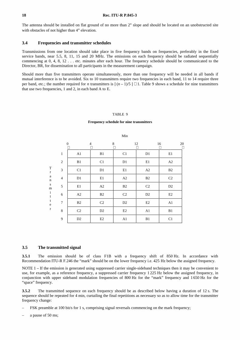
Should more than five transmitters operate simultaneously, more than one frequency will be needed in all bands ifmutual interference is to be avoided. Six to 10 transmitters require two frequencies in each band, 11 to 14 require threeper band, etc.; the number required for n transmitters is | (n – 1)/5 | + 1. Table 9 shows a schedule for nine transmittersthat use two frequencies, 1 and 2, in each band A to E.

TABLE 9

Frequency schedule for nine transmitters

3.5 The transmitted signal

3.5.1 The emission should be of class F1B with a frequency shift of 850 Hz. In accordance withRecommendation ITU-R F.246 the “mark” should be on the lower frequency i.e. 425 Hz below the assigned frequency.

NOTE 1 – If the emission is generated using suppressed carrier single-sideband techniques then it may be convenient touse, for example, as a reference frequency, a suppressed carrier frequency 1 225 Hz below the assigned frequency, inconjunction with upper sideband modulation frequencies of 800 Hz for the “mark” frequency and 1 650 Hz for the“space” frequency.

3.5.2 The transmitted sequence on each frequency should be as described below having a duration of 12 s. Thesequence should be repeated for 4 min, curtailing the final repetitions as necessary so as to allow time for the transmitterfrequency change:

– FSK preamble at 100 bit/s for 1 s, comprising signal reversals commencing on the mark frequency;

– a pause of 50 ms;

Min

0

4

8

12

16

20

1 A1 B1 C1 D1 E1

2 B1 C1 D1 E1 A2

Tr 3 C1 D1 E1 A2 B2

an 4 D1 E1 A2 B2 C2

sm 5 E1 A2 B2 C2 D2

it 6 A2 B2 C2 D2 E2

te 7 B2 C2 D2 E2 A1

r 8 C2 D2 E2 A1 B1

9 D2 E2 A1 B1 C1

Rec. ITU-R P.845-3 19

– an identification signal in Morse code on the higher frequency (see Recommendation ITU-R F.246) containedwithin a period not exceeding 3.3 s:

– the ratios of lengths within the Morse code sequence shall be in the following ratios:

– dot element length 1 unit

– dash element length 3 units

– space between elements within a character 1 unit

– space between characters of the call sign 3 units

– the length of the unit for the dot element length, etc., shall be a greatest multiple of 100 ms, so that, to thegreatest extent possible, the call sign fills the 3.3 s time available; the call sign shall commence at thebeginning of the available period, with any unused time at the end of the period;

– if permissible this identification signal could with advantage be based on the international locator code used byradio amateurs, provided that the signal can be contained within the period specified;

– a pause of 50 ms;

– a 256-bit complementary sequence transmitted at 1 200 bit/s as follows:

Sequence 1:

1110010000101000000101001101100000011011001010001110101111011000000110111101011100010100110110001110010011010111111010111101100000011011110101111110101100100111000110110010100011101011110110001110010000101000111010110010011111100100110101111110101111011000

– a pause of 50 ms;

– a second 256-bit complementary sequence transmitted at 1 200 bit/s, as follows:

Sequence 2:

0001101111010111111010110010011111100100110101110001010000100111000110111101011100010100110110001110010011010111111010111101100011100100001010000001010011011000111001001101011100010100001001111110010000101000111010110010011111100100110101111110101111011000

– a pause of 50 ms;

– a series of FSK reversals, comprising 273 bits at 100 bit/s, commencing on the lower frequency;

– a 127 bit Gold code identifier sequence, at 100 bit/s, commencing on the lower frequency. The sequences to be usedby each transmitting station taking part in the campaign may be obtained from the BR. The Bureau will also advisereceiving stations of the sequences in use;

– a constant signal on the higher frequency for a duration of at least 3 s, which should continue until the total time forthe sequence is 12 s.

NOTE 2 – The automatic identifier takes the form of a Gold code, length 127 bits, obtained using the following 7 stageshift-register generator algorithm:

s1 = x7 + x3 + x

s2 = x7 + x3 + x2 + x + 1

the sequences successively assigned to transmitter stations should be in the order:

s1 ; s2 ; (s1 + s2); (s1 + τ · s2); ......(s1 + τ126 · s2)

where τn represents a cyclic shift of n places.

3.6 Log-keeping

Detailed logs containing information on the status of the transmitter and particularly on the transmitter power should becompleted at all sites and should be forwarded periodically to the Director, BR.

20 Rec. ITU-R P.845-3

4 Receiver

4.1 Receiver locations

There should be as many receiving stations for the recording of the nine proposed transmitters as possible. Due to thenull in the elevation pattern of vertical transmitting antennas, measurements should not be made at ranges shorter thanabout 500 km.

4.2 Antennas and siting

Short vertical active antennas are recommended for use with field-strength measurements according to the specificationsgiven in Appendix 1. The antennas should be installed on flat ground of no more than 2° slope and should be located onan unobstructed site of at least 25 m radius, with more distant obstacles not higher than 4° elevation, measured at groundlevel. The antenna should be situated away from electric power lines and other metallic structures. The antenna may beprotected against damage by a wooden fence or stockade not higher than 2 m at a distance of at least 3 m. It is preferablethat the site should be in an area of good and homogeneous ground conductivity; in any case the conductivity needs to beknown for use in the analysis of results.

4.3 Receiver specifications and calibration

The field-strength measuring receiver should meet the following minimum performance requirements:

– synthesizer control (10 Hz step);

– external bus available for computer control;

– frequency accuracy ±1 part in 106;

– synthesizer noise sidebands: reciprocal mixing performance better than 70 dB in a bandwidth of 3 kHz at 20 kHzoffset;

– sensitivity SSB 1.0 µV terminated for at least 10 dB (S + N ) / N for a bandwidth of 3 kHz;

– unwanted spurious responses (e.g. image, IF) better than 70 dB;

– selectivity: approximately 3 kHz bandwidth, shape factor (– 60 dB to – 6 dB) 2:1;

– linearity: 3rd-order intercept, 20 kHz spacing, +10 dBm;

– true average measuring capability within 4 s;

– timing accuracy within the receiver system should be maintained within 1 s.

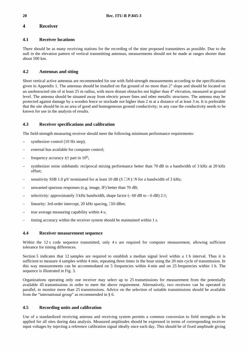
4.4 Receiver measurement sequence

Within the 12 s code sequence transmitted, only 4 s are required for computer measurement, allowing sufficienttolerance for timing differences.

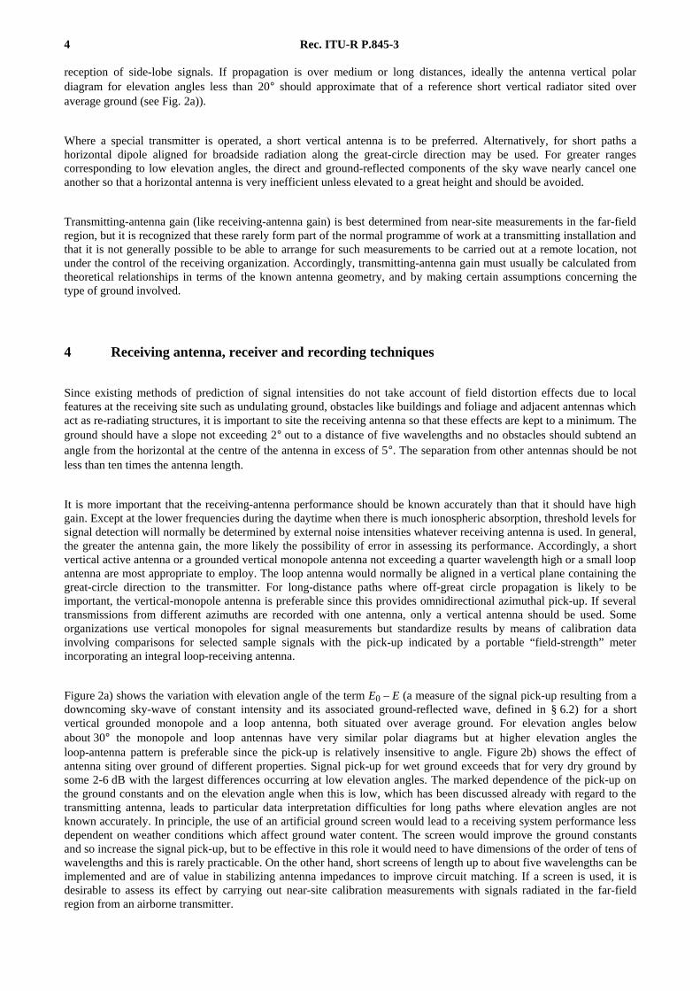
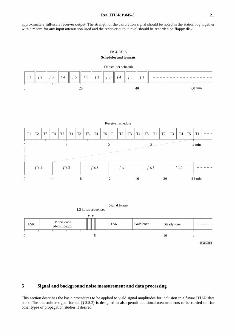
Section 5 indicates that 12 samples are required to establish a median signal level within a 1 h interval. Thus it issufficient to measure 4 samples within 4 min, repeating three times in the hour using the 20 min cycle of transmission. Inthis way measurements can be accommodated on 5 frequencies within 4 min and on 25 frequencies within 1 h. Thesequence is illustrated in Fig. 3.

Organizations operating only one receiver may select up to 25 transmissions for measurement from the potentiallyavailable 45 transmissions in order to meet the above requirement. Alternatively, two receivers can be operated inparallel, to monitor more than 25 transmissions. Advice on the selection of suitable transmissions should be availablefrom the “international group” as recommended in § 6.

4.5 Recording units and calibration

Use of a standardized receiving antenna and receiving system permits a common conversion to field strengths to beapplied for all sites during data analysis. Measured amplitudes should be expressed in terms of corresponding receiverinput voltages by injecting a reference calibration signal ideally once each day. This should be of fixed amplitude giving

Rec. ITU-R P.845-3 21

approximately full-scale receiver output. The strength of the calibration signal should be noted in the station log togetherwith a record for any input attenuation used and the receiver output level should be recorded on floppy disk.

0845-03

0 20 40 60

0 4 8 12 16 20 24

T1 T2 T3 T4 T5 T1 T2 T3 T4 T5 T1 T2 T3 T4 T5 T1 T2 T3 T4 T5 T1

1f 2f 3f 4f 5f 1f 2f 3f 4f 5f 1f

0 1 2 3 4

s 2’f s 3’f s 4’f s 5’f s 1’fs 1’f

0 5 10 s

Transmitter schedule

FIGURE 3

Schedules and formats

Receiver schedule

min

min

min

Signal format1.2 kbit/s sequences

FSKMorse code

identificationFSK Steady toneGold code

FIGURE 3/PI.845 [D03] = 16,5 cm

5 Signal and background noise measurement and data processing

This section describes the basic procedures to be applied to yield signal amplitudes for inclusion in a future ITU-R databank. The transmitter signal format (§ 3.5.2) is designed to also permit additional measurements to be carried out forother types of propagation studies if desired.

22 Rec. ITU-R P.845-3

5.1 Sampling

For each selected circuit (transmitter/receiver/frequency combination) the receiver records sufficient amplitude sampleswithin each hour to permit statistically meaningful estimates of the hourly medians of both the signal and noiseintensities to be determined in relation to the likely within-an-hour fading. Using either analogue or digital signalprocessing, average voltage amplitudes over a period of 4 s within each 12 s transmission cycle should first bedetermined. A minimum of 12 such samples within a given hour on a given day should be taken, these to be distributedapproximately uniformly over the period that the transmitter is radiating. This results in a standard error due to samplingof less than 2 dB.

5.2 Input attenuation

To allow for the varying signal amplitude on different circuits and at different times of day, it is suggested that aswitched attenuator under computer control may be inserted between antenna and receiver, values of attenuation to berecorded on floppy disk along with the signal and noise data.

5.3 Data recording

Data should be dumped to floppy disk in an agreed format (Appendix 2). Hourly medians are to be calculated centrally.Rules for dealing with samples in which the signal is not discernable from noise and interference are given inAppendix 3.

5.4 Determination of monthly medians and deciles

Monthly medians and upper and lower decile values of signal amplitude should be calculated by combining together thehourly median signal-amplitude data at a given hour for the different days. Rules for dealing with daily samples in whichthe signal is below the noise are given in Annex 1.

5.5 Data normalization

Data provided from the separate receiving sites should be accompanied by corresponding receiver and antenna systemcalibration factors for each circuit. Using this information together with that from the transmitter logs, centralized datanormalization will be applied to the different daily/hourly values for incorporation in the data bank.

6 Data handling, quality assurance and training

The scheme envisages a large number of receiving locations (some operating in areas where there is a severe shortage ofskilled engineers), with a large quantity of data, probably in floppy-disk format, being sent to a central agency forcompilation and processing. Such a scheme will work only if adequate attention is given to organization and training.

It is recommended that an international group should be set up to oversee the measurement programme and to provideguidance and assistance to participants. It is further recommended that ITU support should be provided to receive andprocess the data in consultation with the group.

The necessary tasks are to:

– collect and validate measured data provided from the different receiving sites;

– create and maintain summary files of daily hourly median field strengths;

– normalize these results in accordance with the known transmitting and receiving system performance, generate adefinitive data bank, and

– arrange training workshops in various parts of the world so as to ensure the satisfactory operation of receivingsystems.

It is recommended that all data recorded by such equipment be forwarded to the Director, BR, to facilitate thedevelopment of a new ITU-R data base of field-strength measurements.

Rec. ITU-R P.845-3 23

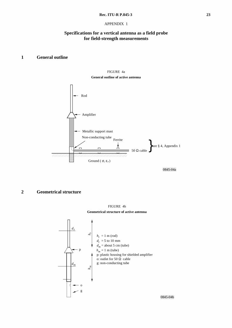
APPENDIX 1

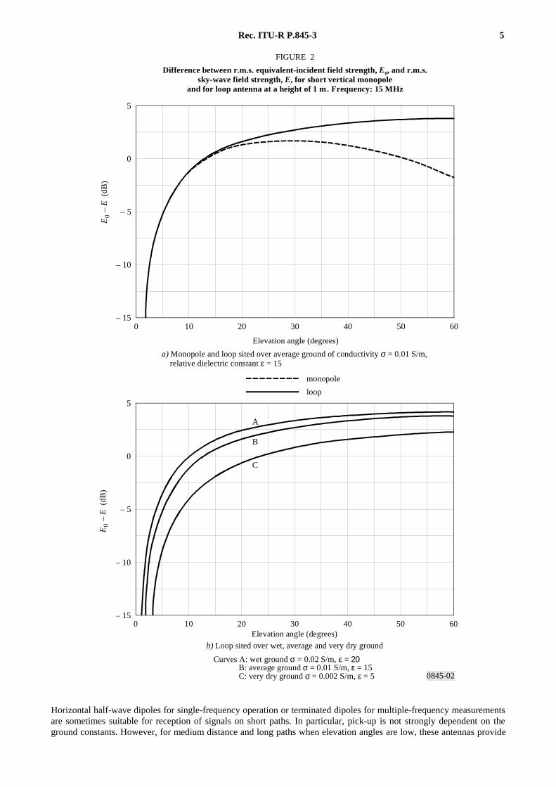
Specifications for a vertical antenna as a field probefor field-strength measurements

1 General outline

0845-04a

Rod

Amplifier

Metallic support mast

Non-conducting tubeFerrite

50 Ω cable

Ground ( σ, ε )r

FIGURE 4a

General outline of active antenna

see § 4, Appendix 1

FIGURE 4a/PI.845 [D04] = 8,5 cm

2 Geometrical structure

0845-04b

hr = 1 m (rod)

dm = about 5 cm (tube)hm = 1 m (tube)p: plastic housing for shielded amplifiero: outlet for 50 Ω cableg: non-conducting tube

dr = 5 to 10 mm

FIGURE 4b

Geometrical structure of active antenna

o

g

dm

hm

p

dr

h r

FIGURE 4b/PI.845 [D05] = 8,5 cm

24 Rec. ITU-R P.845-3

3 Amplifier of active antenna

3.1 Basic schematic

For example an FET source follower and bipolar emitter follower could be used. The d.c. power could be fed throughthe inner conductor of the coaxial cable.

0845-05

Metallic support mast

Non-conducting tube

Vout

Rod

Vi50 Ω

Rod

ViCi

50 Ω50 Ω

VoutRout

FIGURE 5

Basic schematic of active antenna

FIGURE 5/PI.845 [D06] = 9.5 cm

3.2 Electric characteristics of active antenna

– Amplification: Vout / Vi ≈ 1/2 = – 6 dB

– Input impedance: Ci = 15 pF

– Output resistance: Rout = 50 Ω, VSWR ≤ 2

– Noise figure measured at output:

Fout ≤ 15 = 11.8 dB

(Available noise power measured at the output of the shielded antenna or at the output of the amplifier when loadedwith CA = 10 pF at the input)

– Linearity range (signal level for 1 dB compression):

Vcomp, out ≥ 1,2 V (at a load of 50 Ω)measured with dummy antenna

– Intermodulation characteristics:

Intercept point 2nd order, measured at the output:

IPOP2 ≥ 50 V (ou 47 dBm) (with dummy antenna)

Intercept point 3rd order, measured at the output:

IPOP3 ≥ 5 V (or 27 dBm) (with dummy antenna)

The intercept points to be measured by the method of two signal generators.

– Dummy antenna for measurements on the amplifier

Rec. ITU-R P.845-3 25

0845-06

50 Ω C = 10 pFA Amplifier

FIGURE 6

FIGURE 6/PI.845 [D07] = 5 cm

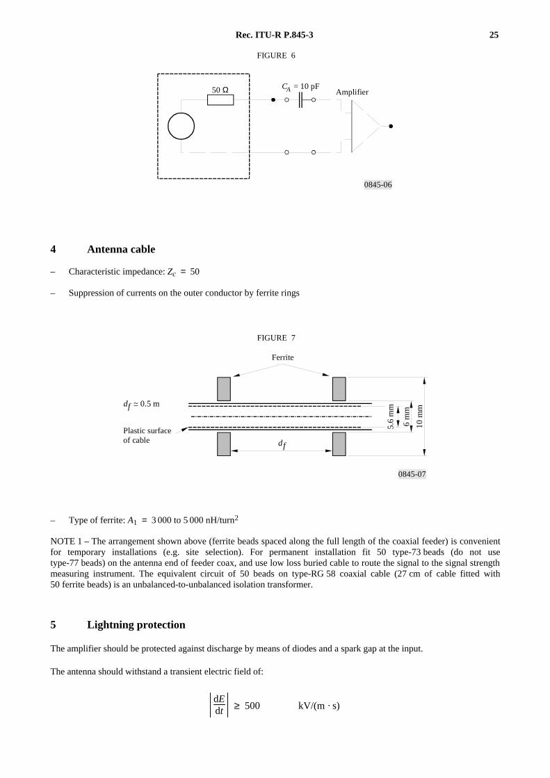
4 Antenna cable

– Characteristic impedance: Zc = 50

– Suppression of currents on the outer conductor by ferrite rings

0845-07

df

10 m

m

6 m

mdf ~ 0.5 m

Ferrite

Plastic surfaceof cable

FIGURE 7

5.6

mm

FIGURE 7/PI.845 [D08] = 5 cm

– Type of ferrite: A1 = 3 000 to 5 000 nH/turn2

NOTE 1 – The arrangement shown above (ferrite beads spaced along the full length of the coaxial feeder) is convenientfor temporary installations (e.g. site selection). For permanent installation fit 50 type-73 beads (do not usetype-77 beads) on the antenna end of feeder coax, and use low loss buried cable to route the signal to the signal strengthmeasuring instrument. The equivalent circuit of 50 beads on type-RG 58 coaxial cable (27 cm of cable fitted with50 ferrite beads) is an unbalanced-to-unbalanced isolation transformer.

5 Lightning protection

The amplifier should be protected against discharge by means of diodes and a spark gap at the input.

The antenna should withstand a transient electric field of:

dEdt ≥ 500 kV/(m · s)

26 Rec. ITU-R P.845-3

APPENDIX 2

Recording of signal and noise amplitudesand related information

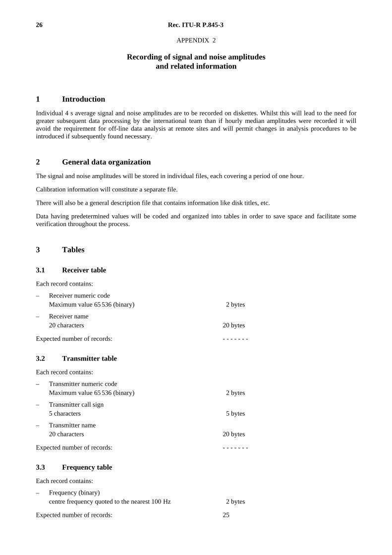
1 Introduction

Individual 4 s average signal and noise amplitudes are to be recorded on diskettes. Whilst this will lead to the need forgreater subsequent data processing by the international team than if hourly median amplitudes were recorded it willavoid the requirement for off-line data analysis at remote sites and will permit changes in analysis procedures to beintroduced if subsequently found necessary.

2 General data organization

The signal and noise amplitudes will be stored in individual files, each covering a period of one hour.

Calibration information will constitute a separate file.

There will also be a general description file that contains information like disk titles, etc.

Data having predetermined values will be coded and organized into tables in order to save space and facilitate someverification throughout the process.

3 Tables

3.1 Receiver table

Each record contains:

– Receiver numeric codeMaximum value 65 536 (binary) 2 bytes

– Receiver name20 characters 20 bytes

Expected number of records: - - - - - - -

3.2 Transmitter table

Each record contains:

– Transmitter numeric codeMaximum value 65 536 (binary) 2 bytes

– Transmitter call sign5 characters 5 bytes

– Transmitter name20 characters 20 bytes

Expected number of records: - - - - - - -

3.3 Frequency table

Each record contains:

– Frequency (binary)centre frequency quoted to the nearest 100 Hz 2 bytes

Expected number of records: 25

Rec. ITU-R P.845-3 27

4 File formats

4.1 General description file

Only one record that contains:

– Title 32 characterscontaining the string

“SG 3 HF measurements”

– Remarks 50 characters(for incorporation of general pertinent information)

4.2 Calibration file

Each record contains:

– Date and time of calibration (binary) 4 bytes

– One calibration signal for all 25 frequencies

1 byte for each frequency 25 bytes

Total 29 bytes

The number of records depends on the number of calibrations that take place during the weekly period (there is onerecord per calibration).

4.3 Measurements file (for each hour and circuit)

– Date and time (binary) 4 bytes

– Transmitter code (binary) 2 bytes

– Frequency identification 1 byte

(index of the frequency tables)

– Input attenuation (dB) 1 byte

– Signal and noise values 12 times (binary)

– Signal amplitude 1 byte

– Signal qualifying or descriptive letter 1 byte

– Noise amplitude 1 byte

Total 44 bytes

5 Diskettes organization

Each diskette will contain data for a period of one week (7 days) consisting of the following:

– 1 general description file

– 1 calibration file

– 168 hourly signal and noise files.

6 Storage considerations

3 ½ in diskettes should be used to collect the data. The data corresponding to one week of recording can beaccommodated on one diskette.

28 Rec. ITU-R P.845-3

7 Remarks

– All receiving stations should register their activity with the international coordination group and be given anidentification code.

– Date and time – a binary number (4 bytes) that contains the elapsed seconds since 00:00:00 UT, 1 January 1970,according to the system clock and permits calculation of the actual date and time.

– Qualifying letters are given in Annex 1.

– Rules for qualifying numerical values as uncertain are given in Annex 1.

– Signal and noise amplitudes will be recorded as integer values.

APPENDIX 3

Rules for determining hourly median signal amplitudes

For a particular circuit there will normally be 12 signal amplitude samples within a given hour on a given day. If allthese samples have unqualified numerical values the median is readily determined by ranking them in ascending orderand taking the average of the two middle numbers.

However, complications arise when some sample values are qualified or are accompanied or replaced by descriptiveletters. The following qualifying and descriptive letters are proposed (see also Annex 1):

D : to indicate that the numerical value is lower than or equal to the true value (as for example when exceedingreceiver full scale)

E : to indicate that the numerical value is greater than or equal to the true value (below the composite backgroundof receiver noise, atmospheric noise and man-made noise and interference)

U : uncertain. A numerical value is classified as uncertain when it is not believed accurate to within ± (2 to 4 dB)

C : no measurement was possible because of technical trouble

S : measurement influenced by or impossible because of interference or atmospherics.

Every measured signal amplitude is accompanied by an associated amplitude of the composite background with which itis compared in selecting letters E and U.

Cases of C or S do not contribute to the signal sample count but numerical values accompanied by qualifying letters do.

When there are some data values accompanied by qualifying letters a first trial median is determined ignoring allqualifying letters. If then it is found that all values accompanied by D are greater than this median and all accompaniedby E are less than this median, then the first trial median is the final median. Otherwise a second trial median is producedby moving all E values to the bottom of the list and all D values to the top. The final median is then the average of thefirst and second trial medians. If these differ by more than 2 dB then the final median is qualified by U.

If more than half of the signal samples are qualified by E (or D) the median is determined in the normal way and is alsoqualified by E (or D).

_________________