
Measurement of Life-Time and -Violation in Polarized Muon...
52
Measurement of μ Life-Time and ˆ P -Violation in Polarized Muon Decay Raffaele Gerosa Badder Marzocchi Luca Mastrolorenzo University of Milano-Bicocca September 19, 2011 Abstract After a characterization of the experimental equipment, the experiment is performed in two stages. In the first one the aim is the μ lifetime measurement in vacuum and in different materials (Al and NaCl), giving the following results: τ =2.193±0.048(stat)±0.058(syst) μs and τ =2.194 ± 0.026(stat) ± 0.145(syst) μs for the vacuum, τ (Al) = 870 ± 93(stat) ± 35(syst) ns and τ (NaCl) = 702 ± 136(stat) ± 52(syst) ns. In the second one, the goal is to probe weak ˆ P -violation through asymmetry oscillation measurement in μ polarized decay in magnetic field. Through this method we manage to exclude within 90% C.L. the absence of asymmetry oscillation and to confirm it within 46.33% χ 2 -significance. 1 Introduction In the first section Sec.1.1, the main features of cosmic muons are presented; then in 1.2 and 1.3 the attention is focused on free and bound muon decay in matter. 1.1 Cosmic Rays Muon is a charged particle belonging to the second leptonic family. It is like the electron except for its rest mass: m μ = 105.6583668 ± 0.0000038 MeV [1] Muons observed in our laboratory have cosmic origin. Cosmic rays are particles coming from outer space and are divided into two main families: ”primary” and ”secondary” cosmic rays. Particles belonging to the primary one have extra-galactic origin and are composed mainly by protons (∼ 95%), He nuclei (∼ 5%) and in a small number of light charged particles and antiparticles. Thus electrons, protons and helium, as well as carbon, oxygen, iron, and other nuclei synthesized in stars, are primaries. It’s possible to estimate their differential energy spectrum, reported in Fig.1, with polinomial functions [2], [3]: dN dE ≈ ( const · E -3.1 E/c < 100 PeV/c const · E -2.7 E/c > 100 PeV/c (1) Particles belonging to the ”secondary” family are generated by interactions of the primaries with interstellar gas, in our specific case with Earth’s upper atmosphere. These interactions create mainly pions ( π + ,π 0 ,π - ) and photons (γ ), minimally kaons ( K + ,K 0 ,K - ) and other particles and nuclei such as lithium, beryllium, and boron. Pions and kaons are unstable particles and 1
Transcript of Measurement of Life-Time and -Violation in Polarized Muon...
Measurement of µ Life-Time and P -Violation in
Polarized Muon Decay
Raffaele Gerosa Badder Marzocchi Luca Mastrolorenzo
University of Milano-Bicocca
September 19, 2011
Abstract
After a characterization of the experimental equipment, the experiment is performed in twostages. In the first one the aim is the µ lifetime measurement in vacuum and in differentmaterials (Al andNaCl), giving the following results: τ = 2.193±0.048(stat)±0.058(syst) µsand τ = 2.194 ± 0.026(stat) ± 0.145(syst) µs for the vacuum, τ(Al) = 870 ± 93(stat) ±35(syst)ns and τ(NaCl) = 702± 136(stat)± 52(syst)ns. In the second one, the goal is toprobe weak P -violation through asymmetry oscillation measurement in µ polarized decay inmagnetic field. Through this method we manage to exclude within 90% C.L. the absence ofasymmetry oscillation and to confirm it within 46.33% χ2-significance.
1 Introduction
In the first section Sec.1.1, the main features of cosmic muons are presented; then in 1.2 and1.3 the attention is focused on free and bound muon decay in matter.
1.1 Cosmic Rays
Muon is a charged particle belonging to the second leptonic family. It is like the electronexcept for its rest mass:
mµ = 105.6583668± 0.0000038MeV [1]
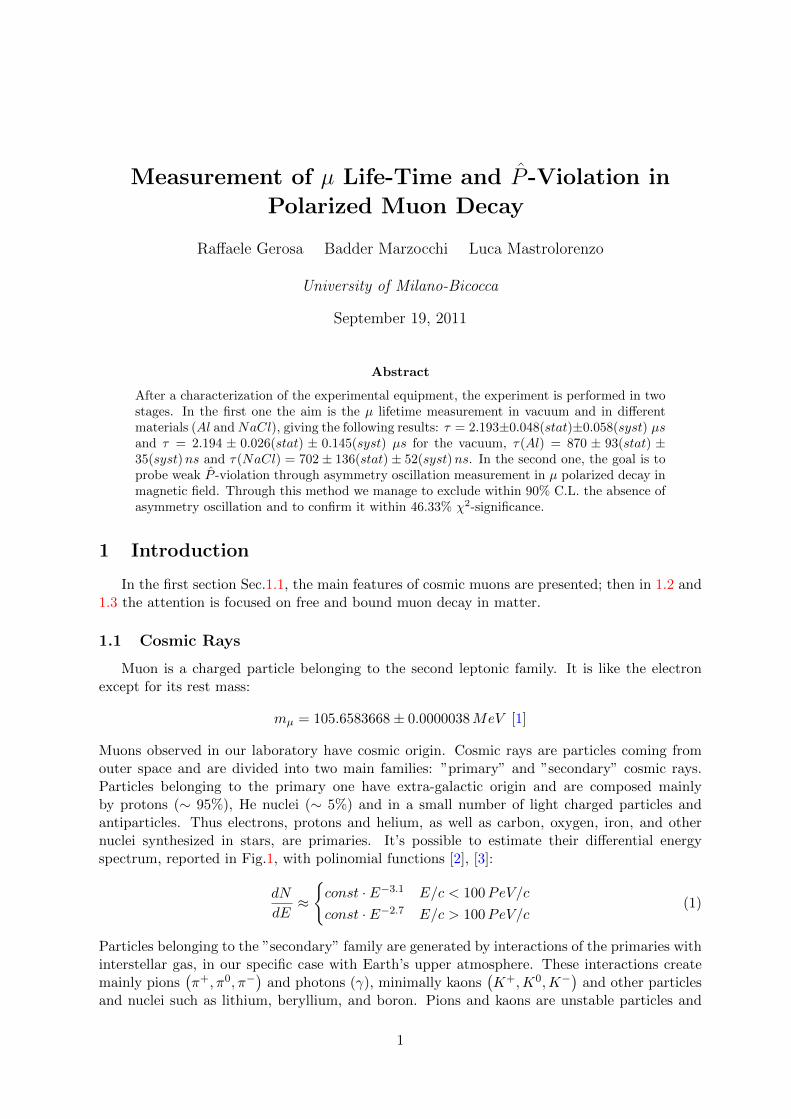
Muons observed in our laboratory have cosmic origin. Cosmic rays are particles coming fromouter space and are divided into two main families: ”primary” and ”secondary” cosmic rays.Particles belonging to the primary one have extra-galactic origin and are composed mainlyby protons (∼ 95%), He nuclei (∼ 5%) and in a small number of light charged particles andantiparticles. Thus electrons, protons and helium, as well as carbon, oxygen, iron, and othernuclei synthesized in stars, are primaries. It’s possible to estimate their differential energyspectrum, reported in Fig.1, with polinomial functions [2], [3]:
dN
dE≈const · E−3.1 E/c < 100PeV/c
const · E−2.7 E/c > 100PeV/c(1)
Particles belonging to the ”secondary” family are generated by interactions of the primaries withinterstellar gas, in our specific case with Earth’s upper atmosphere. These interactions createmainly pions
(π+, π0, π−
)and photons (γ), minimally kaons
(K+,K0,K−
)and other particles
and nuclei such as lithium, beryllium, and boron. Pions and kaons are unstable particles and
1
1.1 Cosmic Rays 2
Energy (eV)
910 1010 1110 1210 1310 1410 1510 1610 1710 1810 1910 2010
-1 s
r GeV
sec
)2
Flux
(m
-2810
-2510
-2210
-1910
-1610
-1310
-1010
-710
-410
-110
210
410
-sec)2(1 particle/m
Knee-year)2(1 particle/m
Ankle-year)2(1 particle/km
-century)2(1 particle/kmFNAL Tevatron (2 TeV)CERN LHC (14 TeV)
LEAP - satellite
Proton - satellite
Yakustk - ground array
Haverah Park - ground array
Akeno - ground array
AGASA - ground array
Fly’s Eye - air fluorescence
HiRes1 mono - air fluorescence
HiRes2 mono - air fluorescence
HiRes Stereo - air fluorescence
Auger - hybrid
Cosmic Ray Spectra of Various Experiments
Figure 1: Spectrum of primary cosmic rays.
decay into lighter ones. These processes form two types of showers: the electromagnetic and thehadronic ones. E.g. we report some of the main reactions:
p+X → π±(0) + Y, π0 → γ + γ, γ → e+ + e−, Y → n+ p, π± → µ± + νµ (νµ)
The majority of the decay products cannot reach the Earth’s surface because they have a tooshort lifetime and not enough energy. On the other hand, most of the muons and all neutrinos,produced by charged pions decay, can easily reach the surface. So, muons are the most plentifulcharged particles at the sea level. They are produced in the high atmosphere (typically 15 km)and they lose about 2 GeV by ionization before reaching the ground. As muon is not the lightestlepton, it decays into:
µ− → e− + νe + νµ µ+ → e+ + νe + νµ
It’s mean free lifetime is reported beneath:
τµ = (2.197034± 0.000021)× 10−6s [1] (2)
Because of the muons are produced at about 15 Km in the atmosphere, they can reach the sealevel only if:
γ =L
cτµ≈ 23 E = m0c
2γ ≈ 2.4GeV(
+ 2GeV loss by ionization)→ E ≥ 4GeV
1.2 Free Muon Decay 3
24. Cosmic rays 7
!""!"! !"""
!""
!"""
!µ####$%&'(")
! µ*+, #$%#! µ
#$-
!*# .!!#./
!!0%&'("1!+,)
Figure 24.4: Spectrum of muons at ! = 0! (! [38], " [43], ! [44], # [45], !,+ [40], " [41], and • [42] and ! = 75! $ [46]) . The line plots the result fromEq. (24.4) for vertical showers.
!+*
!+!
!+2
!+3
!+4
!+5
!"*!"!+" !"2 !"3
678892:
;<=>8
!µ####$%&'(")
& µ+%&
µ!
Figure 24.5: Muon charge ratio as a function of the muon momentum fromRefs. [41,42,48].
July 30, 2010 14:36
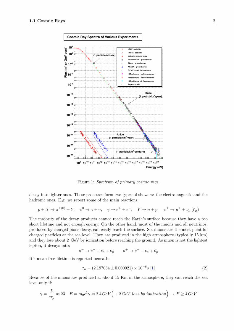
Figure 2: Left: spectrum of muons at θ = 75 (♦) and θ = 0 (all the other symbols)[1]. Right:cosmic muons charge asymmetry, measured at sea level [1].
The mean energy of muons at the ground is approximately 4 GeV, as reported in [1]. Theenergy spectrum over 1 GeV is shown in Fig.2, whereas it is almost flat below 1 GeV. The fluxof vertical muons above 1 GeV at the sea level is
φµ(θ = 0) ≈ 1 cm−2min−1 [1]. (3)
The angular distribution at sea level for muons with energy above 3 GeV is:
dN
dΩdAdt≈ I0 cos2 θ I0 ≈ 100m−2sr−1s−1 (4)
Another important feature of cosmic muons is their measured charge asymmetry, reported inFig.2. This asymmetry is due to the excess of protons over neutrons in the primary spectrum,which brings an overabundance of π+ over π−.
1.2 Free Muon Decay
This is a fully leptonic process in which a muon ( qµ = e and momentum pµ) is convertedinto an electron (me = 0.511 MeV, pe) through the emission of two neutrinos (pνe , pνµ):
µ− −→ e− + νe + νµ or µ+ −→ e+ + νe + νµ
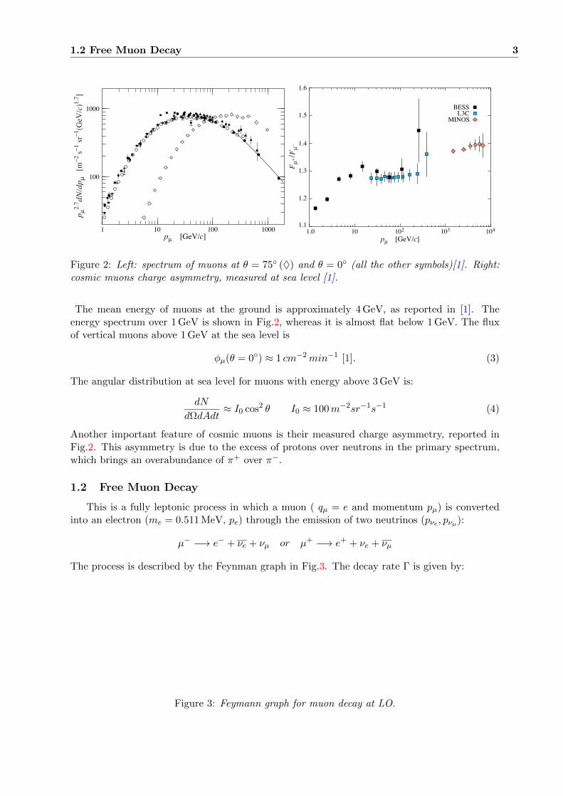
The process is described by the Feynman graph in Fig.3. The decay rate Γ is given by:
Figure 3: Feymann graph for muon decay at LO.
1.3 Bound Muon Decay 4
dΓ = (2π)4δ4(pµ −
∑f
pf
) 1
2Eµ
∏f
d3pf(2π)32Ef
∑f
|M |2 (5)
where f=1,2,3 is the final state particles index (e, νe and νµ). The amplitude M follows fromthe Feynman rules. Making all the calculations described in Appendix A:
Γ =G2fm
5µ
192π3=⇒ τ [µ± → e+ νe + νµ] = 2.2µs (6)
A most accurate value for τµ is calculated taking into account: the electron mass, providing
correction of order m2e/m
2µ for Γ, the Q.E.D radiative correction Γ(1) = Γ(0)
[1− α
2π (π2 − 254 ) +
O(α2)]
and the B.R. of this decay mode (0.9986, against the 1.4 · 10−2 of the channel e−νµνeγ
[1]). After that, the Standard Model prediction for µ lifetime is consistent with the experimentalmeasurements reported in Eq.2.
1.3 Bound Muon Decay
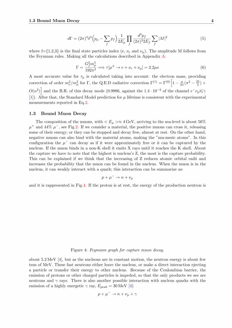
The composition of the muons, with < Eµ >≈ 4 GeV, arriving to the sea-level is about 56%µ+ and 44% µ−, see Fig.2. If we consider a material, the positive muons can cross it, releasingsome of their energy; or they can be stopped and decay free, almost at rest. On the other hand,negative muons can also bind with the material atoms, making the ”mu-mesic atoms”. In thisconfiguration the µ− can decay as if it were approximately free or it can be captured by thenucleus. If the muon binds in a non-K shell it emits X rays until it reaches the K shell. Aboutthe capture we have to note that the highest is nucleus’s Z, the most is the capture probability.This can be explained if we think that the increasing of Z reduces atomic orbital radii andincreases the probability that the muon can be found in the nucleus. When the muon is in thenucleus, it can weakly interact with a quark; this interaction can be summarize as:
p+ µ− → n+ νµ
and it is rappresented in Fig.4. If the proton is at rest, the energy of the production neutron is
Figure 4: Feymann graph for capture muon decay.
about 5.2 MeV [4], but as the nucleons are in constant motion, the neutron energy is about fewtens of MeV. These fast neutrons either leave the nucleus, or make a direct interaction ejectinga particle or transfer their energy to other nucleus. Because of the Coulombian barrier, theemission of protons or other charged particles is impeded, so that the only products we see areneutrons and γ rays. There is also another possible interaction with nucleus quarks with theemission of a highly energetic γ ray, Epeak = 30 MeV [4]:
p+ µ− → n+ νµ + γ
1.3 Bound Muon Decay 5
This process is rare, indeed [4]:
R =ΓRadΓC
≈ 10−4
where ΓRad is radiative capture rate and ΓC is non-radiative one. Because of quarks interactionsat low energies, the theoretical description of muon capture is very difficult and strongly modeldependent. A theoretical description of this phenomenon is beyond this report goal. If ΓC(Z) isnon-radiative capture rate and ΓD(Z) is the decay rate without nuclear interaction in µ-mesicatoms, we have:
Γ(Z) = ΓC(Z) + ΓD(Z) τ− =1
Γ(Z)(7)
As we know, these rates depend on nucleus Z. For low Z → ΓD ≈1
τ+, whereas for high Z we
have to take into account a lot of other effects. Firstly, the total energy of the bound negativemuon is less than the total energy of the free positive muon because of the binding energy.Consequently the phase space is reduced, decreasing the decay probability. Secondly the effectof the nuclear Coulomb field may influence the decay probability. Finally, the motion of negativemuon in the K shell gives rise to a relativistic change in the time scale, increasing the life-timein the lab. An estimation of the ΓD(Z) decreasing is:
ΓD(Z) ≈[
1− ρ(Z
137
)2]· ΓD(0) [4] (8)
where ρ ≈ 3; this is valid for Z < 137√ρ . About ΓC(Z) we can say that greater Z decreases orbital
radii and increases nucleus dimension, so that the nucleus point-charge approximation becomesimpossible. An estimation of this effect is given by Primakoff law [4]:
Zeff = Z
[1 +
(Z
42
)1.47]− 1
1.47
(9)
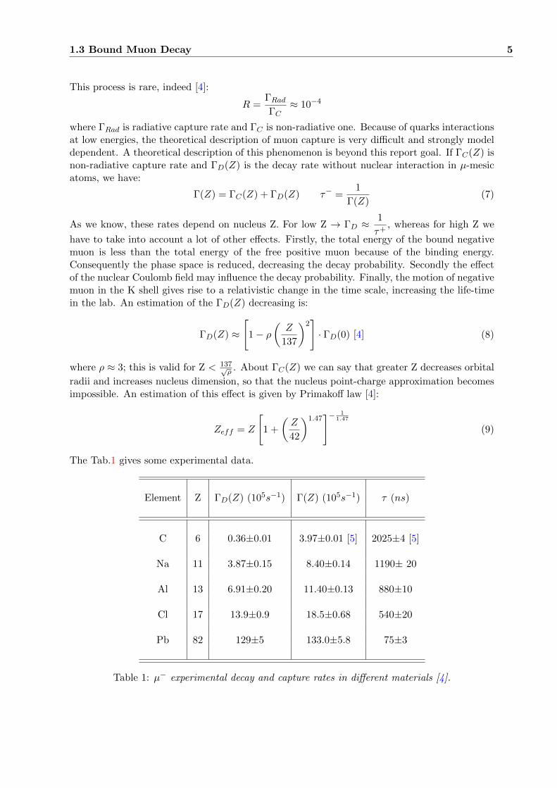
The Tab.1 gives some experimental data.
Element Z ΓD(Z) (105s−1) Γ(Z) (105s−1) τ (ns)
C 6 0.36±0.01 3.97±0.01 [5] 2025±4 [5]
Na 11 3.87±0.15 8.40±0.14 1190± 20
Al 13 6.91±0.20 11.40±0.13 880±10
Cl 17 13.9±0.9 18.5±0.68 540±20
Pb 82 129±5 133.0±5.8 75±3
Table 1: µ− experimental decay and capture rates in different materials [4].
2 Experimental Equipment 6
2 Experimental Equipment
The aim of the experiment is to perform only time measurements, thus we need a detectorable to provide a very fast response to the passage of a particle O(ns). The precision of a timemeasurement is in general determined by two main factors:
• Time Jitter: it is the time dispersion of the signal caused by random effect in its formation.It is irreducible and cannot be corrected.
• Threshold Walk: it is the dispersion of the threshold crossing time due to signal amplitudefluctuations.
Knowing that, for fast detector we mean a detector producing a signal with a low jitter andshort rise-time, which can give a usable information in a very short time. The simplest and mostwidely used detectors of this class are the organic scintillators, which have low density ρ ≈ 1g/cm3 and a fast response time ≈ ns.In this experiment we use three organic plastic scintillators 4.25× 30.30× 80.50 cm 1. Each oneis coupled to a photomultiplier tube through a wavelength shifter. Moreover, the electronicsused for the processing of the signal extracted at the anode of each PM is:
• One Crate NIM.
• One 8-Channel Low-Threshold Discriminator2.
• Quad logic Fan-in/Fan-out.
• One 4-fold programmable logic unit with veto3.
• One Dual Timer (Caen N93B).
• One Octal Gate and Delay Generator (Ortec GG8020).
• One Quad Coincidence Unit4.
• One NIM 4-Channel Programmable Power Supply5.
• Onw DC Power Supply SPS-1230, 12V-30A, GW INSTEK
• One two-channel digital oscilloscope with GPIB output.
• One PC for data acquisition and processing.
2.1 Interaction Muon-Scintillator
As reported in Sec.1.1, muons reach the ground with a mean energy of < Eµ >≈ 4 GeV.When they cross an absorber, such as a scintillator, they lose some of their energy thanks toscattering events with the internal electrons. The energy loss per unit length, called stoppingpower, for a massive charged particle (mµ >> me) is given by the Bethe-Block equation [6]:
−dEdx
= 4π NAρZ
A
e4z2
mev2
[ln(2mec
2β2γ2
I
)− β2 − δ
2
](10)
1http : //www.detectors.saint−gobain.com/uploadedF iles/SGdetectors/Documents/ProductDataSheets/BC400−404− 408− 412− 416−Data− Sheet.pdf
2CAEN model N 417, http://www.caentechnologies.com/csite/SpecialCodes.jsp3 N405 Triple 4-Fold Logic Unit/Majority with VETO4LeCroy 622 Quad 2 Input Logic Unit, http://www.lecroy.com/lrs/dsheets/365al.htm5CAEN N470 HV Power Supply, htpp://www.caentechnologies.com/csite/CaenProd.jsp?parent=21&idmod=238
2.1 Interaction Muon-Scintillator 7
Considering a muon of energy in the order of GeV in interaction with an organic material Z ≈ 6,ρ ≈ 1 g/cm3, it is in condition of M.I.P:
−dEdx≈ 1.5
MeV
cm
Only a fraction of the total energy released [∆E ≈ 1.5MeVcm · 4cm = 6 MeV] excites molecu-
lar levels of the scintillating organic compound, which then rapidly de-excites O(ns) emittingUV photons. In a typical organic scintillator, visible photons [300 − 700 nm] are obtained byconverting the primary light thanks to a wavelength shifter with a rate of 1γ/100 eV, obtaining≈ 60000 γs. Consider that our light collection system is such to allow that 25% [6] of them reachthe photocathode. Here the conversion of the light into electrons, by means of photoelectric ef-fect, has a < Q.E. >≈ 20% [6] over the entire spectrum of collected photons. Thus the number ofphotoelectrons that reach the stage of multiplication in the tube are: Ne ≈ 60000·0.25·0.2 = 3000Assuming that the number of obtained electrons are Poisson distributed:
P (n,Ne) =(Ne)
ne−Ne
n!→ P (0, Ne) = e−3000 ≈ 0
Thanks to some simple approximation, our model 4 cm thick plastic scintillator has a intrinsicefficiency of 100% to detect M.I.P. particles. If we have a traditional PM tube with 10 stagesand a dynode gain δ ≈ 4 (note that the gain is strictly connected to the voltage supply ≈ 103V )and considering that the PM pulse travels in a cable with R = 50Ω of impedance:
G ≈ δN = 410 → ∆V ≈ Ne · e ·G∆t(≈ 100ns)
·R ≈ 250mV, ∆V (1e−) ≈ 0.084mV
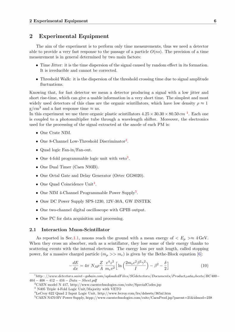
This result is consistent with the amplitude of our PM output signals produced by the interactionbetween the muon and the detector, as shown in Fig.5.
Figure 5: Muon waveform taken from the oscilloscope.
3 Scintillators Characterization 8
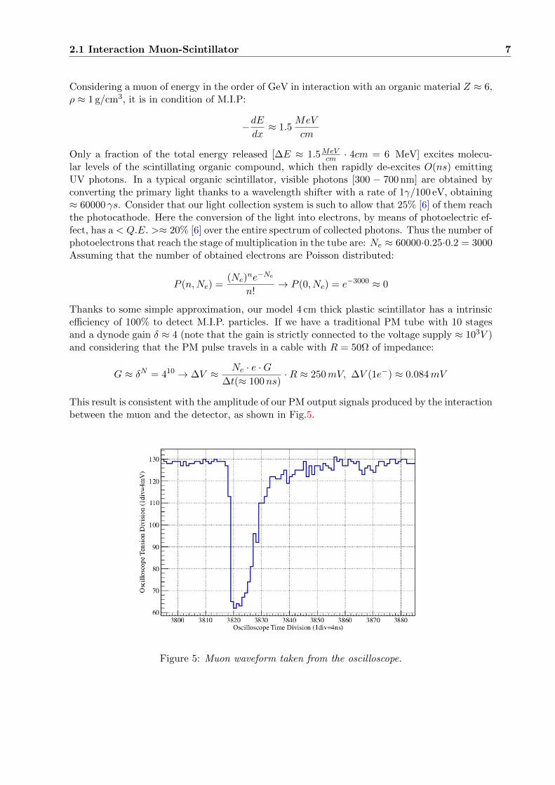
Figure 6: Electron waveform taken from the oscilloscope.
3 Scintillators Characterization
Before setting up the experimental apparatus, we characterize the three scintillators effi-ciency. Since whichever configuration for time measurement needs a trigger, we have also tostudy thresholds.
3.1 Thresholds and Biases
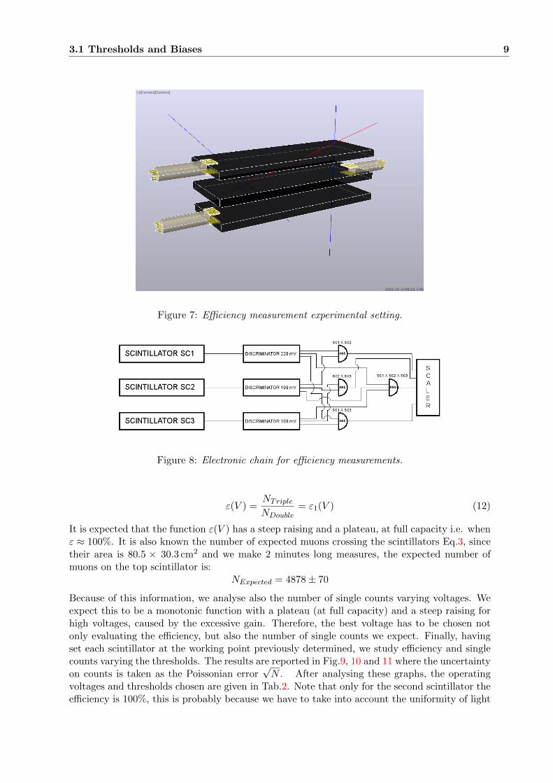
Our goal consists of determining, for each scintillator, the working point and the triggerthreshold in order to optimize scintillators efficiency. At first, for each scintillator the voltageis fixed at the value of 1 KV. Then, we analyse the signal waveforms to choose a suitablethreshold value. The waveforms have a maximum amplitude of Vmax ≈ 600 mV for SC1 (itstands for scintillator number one) and Vmax ≈ 350 mV for SC2 and SC3. Thus, the followingthresholds are chosen: 220 mV→SC1 and 100 mV→ SC2 and SC3. The efficiency measurementis based on counting muons crossing the different scintillators, using the configuration shown inFig.7. The scintillators are put one upon the other, with spacings of 10 cm. After choosing thescintillator to analyse, we fix the other voltages and vary that scintillator bias. Our aim is tomake double-coincidences and triple-coincidences using the electronic chain described in Fig.8.In this configuration the efficiency, ε is defined as:
ε(V ) =NTriple
NDouble(11)
where NDouble is the number of double-coincidences between the bias-fixed scintillators andNTriple is the number of coincidences among all of them. The width of the coincidence gate i.e.the width of the logic pulses produced by the discriminator is fixed to 100 ns. Note that withthis method we don’t need the bias-fixed scintillators to have 100% efficiency. For example, ifwe vary the SC1 bias:
NDouble = NTOT · ε2 · ε3
NTriple = NTOT · ε1(V ) · ε2 · ε3
3.1 Thresholds and Biases 9
Figure 7: Efficiency measurement experimental setting.
Figure 8: Electronic chain for efficiency measurements.
ε(V ) =NTriple
NDouble= ε1(V ) (12)
It is expected that the function ε(V ) has a steep raising and a plateau, at full capacity i.e. whenε ≈ 100%. It is also known the number of expected muons crossing the scintillators Eq.3, sincetheir area is 80.5 × 30.3 cm2 and we make 2 minutes long measures, the expected number ofmuons on the top scintillator is:
NExpected = 4878± 70
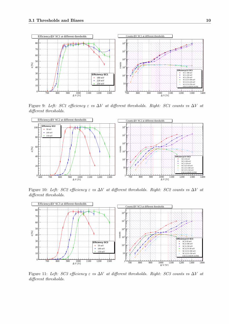
Because of this information, we analyse also the number of single counts varying voltages. Weexpect this to be a monotonic function with a plateau (at full capacity) and a steep raising forhigh voltages, caused by the excessive gain. Therefore, the best voltage has to be chosen notonly evaluating the efficiency, but also the number of single counts we expect. Finally, havingset each scintillator at the working point previously determined, we study efficiency and singlecounts varying the thresholds. The results are reported in Fig.9, 10 and 11 where the uncertaintyon counts is taken as the Poissonian error
√N . After analysing these graphs, the operating
voltages and thresholds chosen are given in Tab.2. Note that only for the second scintillator theefficiency is 100%, this is probably because we have to take into account the uniformity of light
3.1 Thresholds and Biases 10
V [V]∆700 800 900 1000 1100 1200 1300
[%
]ε
0
10
20
30
40
50
60
70
80
V SC1 at different thresholds∆Efficiency/
Efficiency SC1180 mV220 mV250 mV
V [V]∆700 800 900 1000 1100 1200 1300 1400
coun
ts
1
10
210
310
410
510
610
V SC1 at different thresholds∆Counts/
V SC1∆Efficiency/SC1-180 mVSC1-220 mVSC1-250 mVSC1/2/3-180 mVSC1/2/3-220 mVSC1/2/3-250 mVEXCLUSION ZONE
Figure 9: Left: SC1 efficiency ε vs ∆V at different thresholds. Right: SC1 counts vs ∆V atdifferent thresholds.
V [V]∆600 700 800 900 1000 1100 1200 1300
[%
]ε
0
20
40
60
80
100
V SC2 at different thresholds∆Efficiency/
Efficiency SC2
50 mV
100 mV
150 mV
V [V]∆700 800 900 1000 1100 1200 1300 1400
coun
ts
1
10
210
310
410
510
610
V SC2 at different thresholds∆Counts/
V SC2∆Efficiency/SC2-50 mVSC2-100 mVSC2-150 mVSC1/2/3-50 mVSC1/2/3-100 mVSC1/2/3-150 mVEXCLUSION ZONE
Figure 10: Left: SC2 efficiency ε vs ∆V at different thresholds. Right: SC2 counts vs ∆V atdifferent thresholds.
V [V]∆700 800 900 1000 1100 1200 1300
[%
]ε
0
10
20
30
40
50
60
70
80
V SC3 at different thresholds∆Efficiency/
Efficiency SC350 mV100 mV150 mV
V [V]∆700 800 900 1000 1100 1200 1300 1400
coun
ts
1
10
210
310
410
510
610
V SC3 at different thresholds∆Counts/
V SC3∆Efficiency/SC3-50 mVSC3-100 mVSC3-150 mVSC1/2/3-50 mVSC1/2/3-100 mVSC1/2/3-150 mVEXCLUSION ZONE
Figure 11: Left: SC3 efficiency ε vs ∆V at different thresholds. Right: SC3 counts vs ∆V atdifferent thresholds.
3.2 Uniformity of Light Yield 11
yield and the geometrical efficiency as well.
Scintillator Threshold Bias Efficiency [%]
SC1 220 mV 900 V 77.26± 2.31
SC2 100 mV 975 V 99.79± 3.12
SC3 100 mV 1025 V 77.19± 2.32
Table 2: Thresholds and biases
3.2 Uniformity of Light Yield
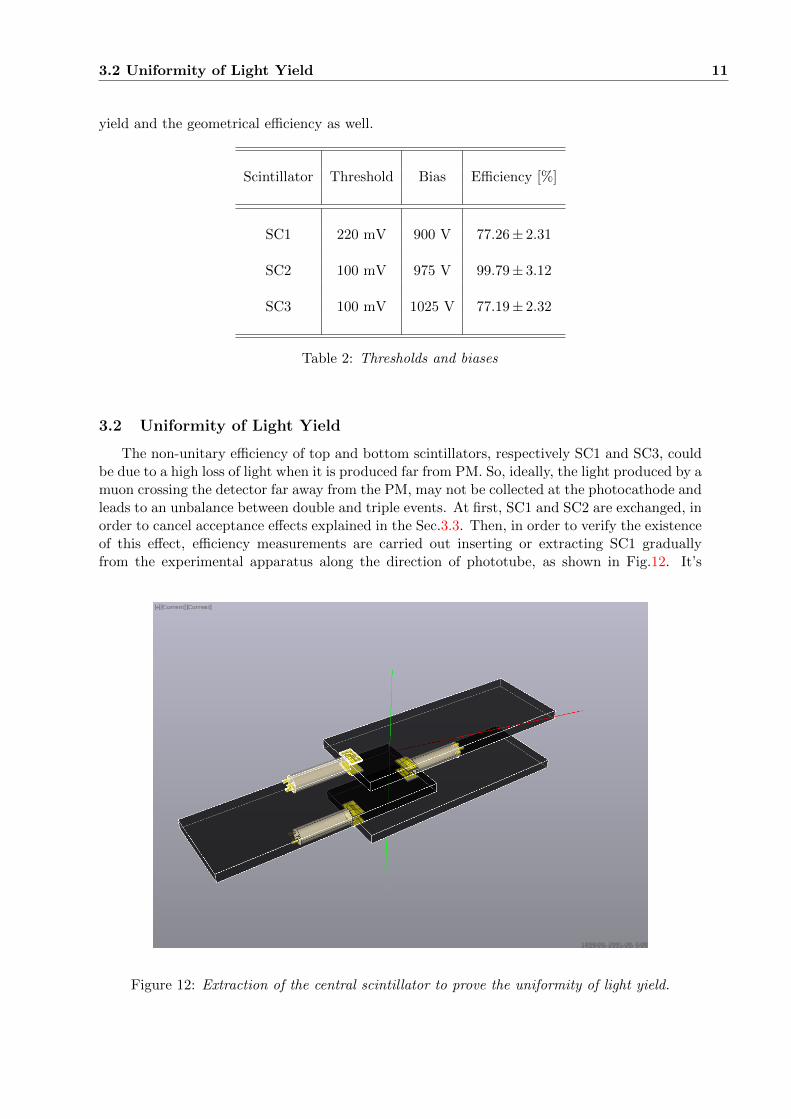
The non-unitary efficiency of top and bottom scintillators, respectively SC1 and SC3, couldbe due to a high loss of light when it is produced far from PM. So, ideally, the light produced by amuon crossing the detector far away from the PM, may not be collected at the photocathode andleads to an unbalance between double and triple events. At first, SC1 and SC2 are exchanged, inorder to cancel acceptance effects explained in the Sec.3.3. Then, in order to verify the existenceof this effect, efficiency measurements are carried out inserting or extracting SC1 graduallyfrom the experimental apparatus along the direction of phototube, as shown in Fig.12. It’s
Figure 12: Extraction of the central scintillator to prove the uniformity of light yield.
3.3 Monte-Carlo Simulation 12
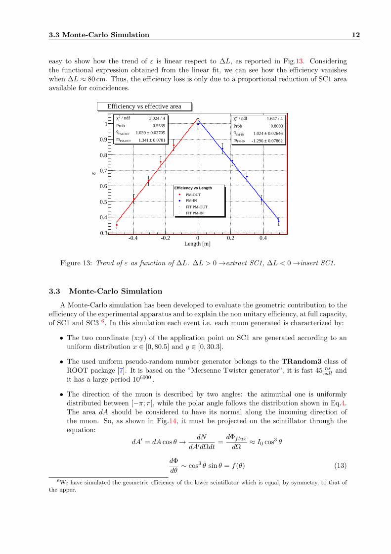
easy to show how the trend of ε is linear respect to ∆L, as reported in Fig.13. Consideringthe functional expression obtained from the linear fit, we can see how the efficiency vanisheswhen ∆L ≈ 80 cm. Thus, the efficiency loss is only due to a proportional reduction of SC1 areaavailable for coincidences.
Length [m]-0.4 -0.2 0 0.2 0.4
ε
0.3
0.4
0.5
0.6
0.7
0.8
0.9
1 / ndf 2χ 3.024 / 4
Prob 0.5539
PM-OUTq 0.02705± 1.039
PM-OUTm 0.0781± 1.341
/ ndf 2χ 3.024 / 4
Prob 0.5539
PM-OUTq 0.02705± 1.039
PM-OUTm 0.0781± 1.341
/ ndf 2χ 1.647 / 4
Prob 0.8003
PM-INq 0.02646± 1.024
PM-INm 0.07862± -1.296
/ ndf 2χ 1.647 / 4
Prob 0.8003
PM-INq 0.02646± 1.024
PM-INm 0.07862± -1.296
Efficiency vs effective area
Efficiency vs Length
PM-OUT
PM-IN
FIT PM-OUT
FIT PM-IN
Figure 13: Trend of ε as function of ∆L. ∆L > 0→extract SC1, ∆L < 0→insert SC1.
3.3 Monte-Carlo Simulation
A Monte-Carlo simulation has been developed to evaluate the geometric contribution to theefficiency of the experimental apparatus and to explain the non unitary efficiency, at full capacity,of SC1 and SC3 6. In this simulation each event i.e. each muon generated is characterized by:
• The two coordinate (x;y) of the application point on SC1 are generated according to anuniform distribution x ∈ [0, 80.5] and y ∈ [0, 30.3].
• The used uniform pseudo-random number generator belongs to the TRandom3 class ofROOT package [7]. It is based on the ”Mersenne Twister generator”, it is fast 45 ns
call andit has a large period 106000 .
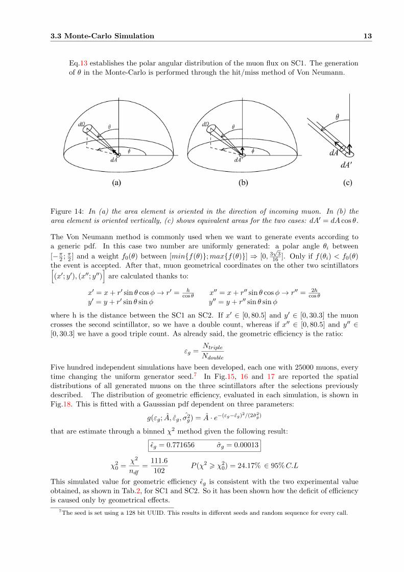
• The direction of the muon is described by two angles: the azimuthal one is uniformlydistributed between [−π;π], while the polar angle follows the distribution shown in Eq.4.The area dA should be considered to have its normal along the incoming direction ofthe muon. So, as shown in Fig.14, it must be projected on the scintillator through theequation:
dA′ = dA cos θ → dN
dA′dΩdt=dΦflux
dΩ≈ I0 cos3 θ
dΦ
dθ∼ cos3 θ sin θ = f(θ) (13)
6We have simulated the geometric efficiency of the lower scintillator which is equal, by symmetry, to that ofthe upper.
3.3 Monte-Carlo Simulation 13
Eq.13 establishes the polar angular distribution of the muon flux on SC1. The generationof θ in the Monte-Carlo is performed through the hit/miss method of Von Neumann.
Figure 14: In (a) the area element is oriented in the direction of incoming muon. In (b) thearea element is oriented vertically, (c) shows equivalent areas for the two cases: dA′ = dA cos θ.
The Von Neumann method is commonly used when we want to generate events according toa generic pdf. In this case two number are uniformly generated: a polar angle θi between
[−π2 ; π2 ] and a weight f0(θ) between [minf(θ);maxf(θ)] ⇒ [0, 3
√3
16 ]. Only if f(θi) < f0(θ)the event is accepted. After that, muon geometrical coordinates on the other two scintillators[(x′; y′), (x′′; y′′)
]are calculated thanks to:
x′ = x+ r′ sin θ cosφ→ r′ = hcos θ x′′ = x+ r′′ sin θ cosφ→ r′′ = 2h
cos θy′ = y + r′ sin θ sinφ y′′ = y + r′′ sin θ sinφ
where h is the distance between the SC1 an SC2. If x′ ∈ [0, 80.5] and y′ ∈ [0, 30.3] the muoncrosses the second scintillator, so we have a double count, whereas if x′′ ∈ [0, 80.5] and y′′ ∈[0, 30.3] we have a good triple count. As already said, the geometric efficiency is the ratio:
εg =Ntriple
Ndouble
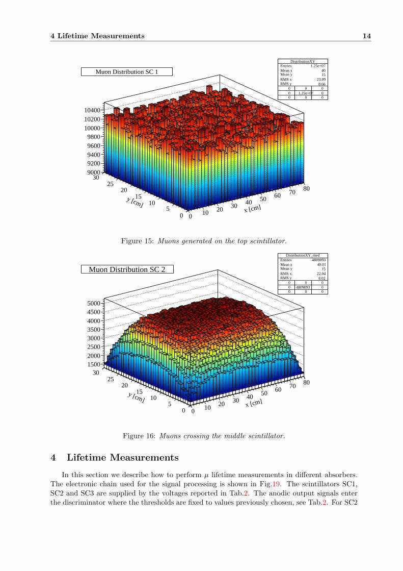
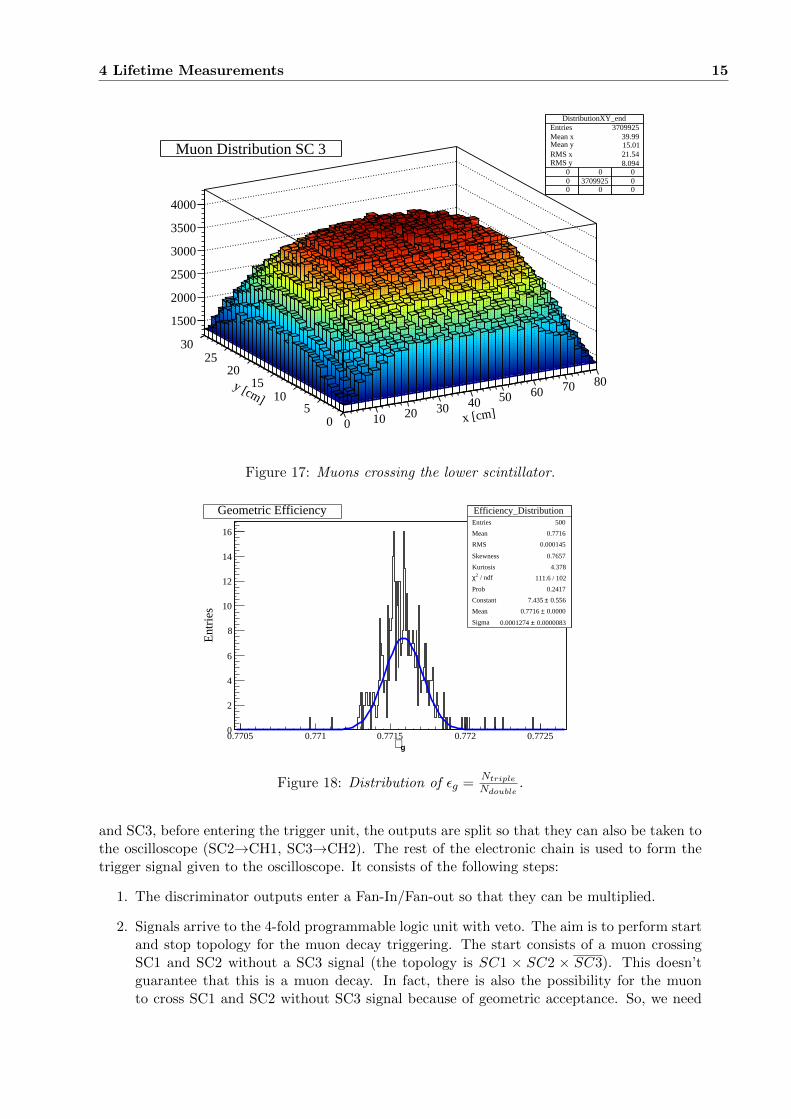
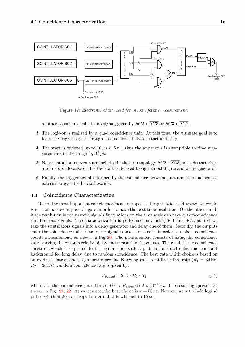
Five hundred independent simulations have been developed, each one with 25000 muons, everytime changing the uniform generator seed.7 In Fig.15, 16 and 17 are reported the spatialdistributions of all generated muons on the three scintillators after the selections previouslydescribed. The distribution of geometric efficiency, evaluated in each simulation, is shown inFig.18. This is fitted with a Gausssian pdf dependent on three parameters:
g(εg; A, εg, σ2g) = A · e−(εg−εg)2/(2σ2
g)
that are estimate through a binned χ2 method given the following result:
εg = 0.771656 σg = 0.00013
χ20 =
χ2
ndf=
111.6
102P (χ2 > χ2
0) = 24.17% ∈ 95%C.L
This simulated value for geometric efficiency εg is consistent with the two experimental valueobtained, as shown in Tab.2, for SC1 and SC2. So it has been shown how the deficit of efficiencyis caused only by geometrical effects.
7The seed is set using a 128 bit UUID. This results in different seeds and random sequence for every call.
4 Lifetime Measurements 14
x [cm]
0 10 20 30 40 50 60 70 80
y [cm]
05
1015
2025
3090009200940096009800
100001020010400
DistributionXYEntries 1.25e+07Mean x 40Mean y 15RMS x 23.09RMS y 8.66 0 0 0 0 1.25e+07 0 0 0 0
DistributionXYEntries 1.25e+07Mean x 40Mean y 15RMS x 23.09RMS y 8.66 0 0 0 0 1.25e+07 0 0 0 0
Muon Distribution SC 1
Figure 15: Muons generated on the top scintillator.
x [cm]
0 10 20 30 40 50 60 70 80
y [cm]
05
1015
2025
3015002000250030003500400045005000
DistributionXY_medEntries 4809093Mean x 40.01Mean y 15RMS x 22.04RMS y 8.02 0 0 0 0 4809093 0 0 0 0
DistributionXY_medEntries 4809093Mean x 40.01Mean y 15RMS x 22.04RMS y 8.02 0 0 0 0 4809093 0 0 0 0
Muon Distribution SC 2
Figure 16: Muons crossing the middle scintillator.
4 Lifetime Measurements
In this section we describe how to perform µ lifetime measurements in different absorbers.The electronic chain used for the signal processing is shown in Fig.19. The scintillators SC1,SC2 and SC3 are supplied by the voltages reported in Tab.2. The anodic output signals enterthe discriminator where the thresholds are fixed to values previously chosen, see Tab.2. For SC2
4 Lifetime Measurements 15
x [cm]0 10 20 30 40 50 60 70 80y [cm]
05
1015
2025
30
1500
2000
2500
3000
3500
4000
DistributionXY_endEntries 3709925Mean x 39.99Mean y 15.01RMS x 21.54RMS y 8.094 0 0 0 0 3709925 0 0 0 0
DistributionXY_endEntries 3709925Mean x 39.99Mean y 15.01RMS x 21.54RMS y 8.094 0 0 0 0 3709925 0 0 0 0
Muon Distribution SC 3
Figure 17: Muons crossing the lower scintillator.
Efficiency_DistributionEntries 500
Mean 0.7716
RMS 0.000145
Skewness 0.7657
Kurtosis 4.378
/ ndf 2χ 111.6 / 102
Prob 0.2417
Constant 0.556± 7.435
Mean 0.0000± 0.7716
Sigma 0.0000083± 0.0001274
g∈0.7705 0.771 0.7715 0.772 0.7725
Ent
ries
0
2
4
6
8
10
12
14
16
Efficiency_DistributionEntries 500
Mean 0.7716
RMS 0.000145
Skewness 0.7657
Kurtosis 4.378
/ ndf 2χ 111.6 / 102
Prob 0.2417
Constant 0.556± 7.435
Mean 0.0000± 0.7716
Sigma 0.0000083± 0.0001274
Geometric Efficiency
Figure 18: Distribution of εg =NtripleNdouble
.
and SC3, before entering the trigger unit, the outputs are split so that they can also be taken tothe oscilloscope (SC2→CH1, SC3→CH2). The rest of the electronic chain is used to form thetrigger signal given to the oscilloscope. It consists of the following steps:
1. The discriminator outputs enter a Fan-In/Fan-out so that they can be multiplied.
2. Signals arrive to the 4-fold programmable logic unit with veto. The aim is to perform startand stop topology for the muon decay triggering. The start consists of a muon crossingSC1 and SC2 without a SC3 signal (the topology is SC1 × SC2 × SC3). This doesn’tguarantee that this is a muon decay. In fact, there is also the possibility for the muonto cross SC1 and SC2 without SC3 signal because of geometric acceptance. So, we need
4.1 Coincidence Characterization 16
Figure 19: Electronic chain used for muon lifetime measurement.
another constraint, called stop signal, given by SC2× SC3 or SC3× SC2.
3. The logic-or is realized by a quad coincidence unit. At this time, the ultimate goal is toform the trigger signal through a coincidence between start and stop.
4. The start is widened up to 10µs ≈ 5 τ+, thus the apparatus is susceptible to time mea-surements in the range [0, 10]µs.
5. Note that all start events are included in the stop topology SC2×SC3, so each start givesalso a stop. Because of this the start is delayed trough an octal gate and delay generator.
6. Finally, the trigger signal is formed by the coincidence between start and stop and sent asexternal trigger to the oscilloscope.
4.1 Coincidence Characterization
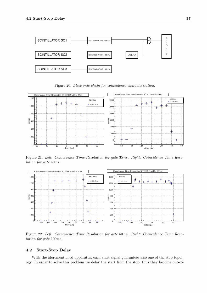
One of the most important coincidence measure aspect is the gate width. A priori, we wouldwant a as narrow as possible gate in order to have the best time resolution. On the other hand,if the resolution is too narrow, signals fluctuations on the time scale can take out-of-coincidencesimultaneous signals. The characterization is performed only using SC1 and SC2; at first wetake the scintillators signals into a delay generator and delay one of them. Secondly, the outputsenter the coincidence unit. Finally the signal is taken to a scaler in order to make a coincidencecounts measurement, as shown in Fig 20. The measurement consists of fixing the coincidencegate, varying the outputs relative delay and measuring the counts. The result is the coincidencespectrum which is expected to be: symmetric, with a plateau for small delay and constantbackground for long delay, due to random coincidence. The best gate width choice is based onan evident plateau and a symmetric profile. Knowing each scintillator free rate (R1 = 32 Hz,R2 = 36 Hz), random coincidence rate is given by:
Rcasual = 2 · τ ·R1 ·R2 (14)
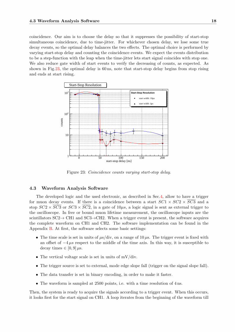
where τ is the coincidence gate. If τ ≈ 100 ns, Rcasual ≈ 2× 10⁻⁴ Hz. The resulting spectra areshown in Fig. 21, 22. As we can see, the best choice is τ = 50 ns. Now on, we set whole logicalpulses width at 50 ns, except for start that is widened to 10µs.
4.2 Start-Stop Delay 17
Figure 20: Electronic chain for coincidence characterization.
s]µdelay [-60 -40 -20 0 20 40 60
coun
ts
0
200
400
600
800
1000
1200SC2⊗ SC1
width: 35 ns
SC2-width: 35ns⊗Coincidence Time Resolution SC1
s]µdelay [-60 -40 -20 0 20 40 60
coun
ts
0
200
400
600
800
1000
1200 SC2⊗ SC1
width: 40 ns
SC2-width: 40ns⊗Coincidence Time Resolution SC1
Figure 21: Left: Coincidence Time Resolution for gate 35ns. Right: Coincidence Time Reso-lution for gate 40ns.
s]µdelay [-80 -60 -40 -20 0 20 40 60 80
coun
ts
0
200
400
600
800
1000
1200
1400 SC2⊗ SC1
width: 50 ns
SC2-width: 50ns⊗Coincidence Time Resolution SC1
s]µdelay [-150 -100 -50 0 50 100
coun
ts
0
200
400
600
800
1000
1200
1400 SC2⊗ SC1
width: 100 ns
SC2-width: 100ns⊗Coincidence Time Resolution SC1
Figure 22: Left: Coincidence Time Resolution for gate 50ns. Right: Coincidence Time Reso-lution for gate 100ns.
4.2 Start-Stop Delay
With the aforementioned apparatus, each start signal guarantees also one of the stop topol-ogy. In order to solve this problem we delay the start from the stop, thus they become out-of-
4.3 Waveform Analysis Software 18
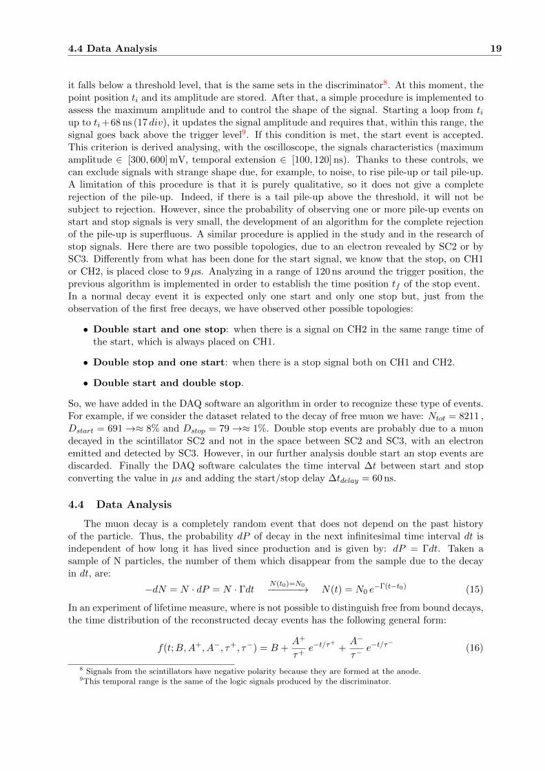
coincidence. Our aim is to choose the delay so that it suppresses the possibility of start-stopsimultaneous coincidence, due to time-jitter. For whichever chosen delay, we lose some truedecay events, so the optimal delay balances the two effects. The optimal choice is performed byvarying start-stop delay and counting the coincidence events. We expect the events distributionto be a step-function with the leap when the time-jitter lets start signal coincides with stop one.We also reduce gate width of start events to verify the decreasing of counts, as expected. Asshown in Fig.23, the optimal delay is 60 ns, note that start-stop delay begins from stop risingand ends at start rising.
start-stop delay [ns]0 50 100 150 200
coun
ts
1
10
210
310
Start-Stop Resolution
Start-Stop Resolution
sµstart width: 10
sµstart width: 1
Figure 23: Coincidence counts varying start-stop delay.
4.3 Waveform Analysis Software
The developed logic and the used electronic, as described in Sec.4, allow to have a triggerfor muon decay events. If there is a coincidence between a start SC1 × SC2 × SC3 and astop SC2 × SC3 or SC3 × SC2, in a gate of 10µs, a logic signal is sent as external trigger tothe oscilloscope. In free or bound muon lifetime measurement, the oscilloscope inputs are thescintillators SC2→ CH1 and SC3→CH2. When a trigger event is present, the software acquiresthe complete waveform on CH1 and CH2. The software implementation can be found in theAppendix B. At first, the software selects some basic settings:
• The time scale is set in units of µs/div, on a range of 10µs. The trigger event is fixed withan offset of −4µs respect to the middle of the time axis. In this way, it is susceptible todecay times ∈ [0, 9]µs.
• The vertical voltage scale is set in units of mV/div.
• The trigger source is set to external, mode edge slope fall (trigger on the signal slope fall).
• The data transfer is set in binary encoding, in order to make it faster.
• The waveform is sampled at 2500 points, i.e. with a time resolution of 4 ns.
Then, the system is ready to acquire the signals according to a trigger event. When this occurs,it looks first for the start signal on CH1. A loop iterates from the beginning of the waveform till
4.4 Data Analysis 19
it falls below a threshold level, that is the same sets in the discriminator8. At this moment, thepoint position ti and its amplitude are stored. After that, a simple procedure is implemented toassess the maximum amplitude and to control the shape of the signal. Starting a loop from tiup to ti+68 ns (17 div), it updates the signal amplitude and requires that, within this range, thesignal goes back above the trigger level9. If this condition is met, the start event is accepted.This criterion is derived analysing, with the oscilloscope, the signals characteristics (maximumamplitude ∈ [300, 600] mV, temporal extension ∈ [100, 120] ns). Thanks to these controls, wecan exclude signals with strange shape due, for example, to noise, to rise pile-up or tail pile-up.A limitation of this procedure is that it is purely qualitative, so it does not give a completerejection of the pile-up. Indeed, if there is a tail pile-up above the threshold, it will not besubject to rejection. However, since the probability of observing one or more pile-up events onstart and stop signals is very small, the development of an algorithm for the complete rejectionof the pile-up is superfluous. A similar procedure is applied in the study and in the research ofstop signals. Here there are two possible topologies, due to an electron revealed by SC2 or bySC3. Differently from what has been done for the start signal, we know that the stop, on CH1or CH2, is placed close to 9µs. Analyzing in a range of 120 ns around the trigger position, theprevious algorithm is implemented in order to establish the time position tf of the stop event.In a normal decay event it is expected only one start and only one stop but, just from theobservation of the first free decays, we have observed other possible topologies:
• Double start and one stop: when there is a signal on CH2 in the same range time ofthe start, which is always placed on CH1.
• Double stop and one start: when there is a stop signal both on CH1 and CH2.
• Double start and double stop.
So, we have added in the DAQ software an algorithm in order to recognize these type of events.For example, if we consider the dataset related to the decay of free muon we have: Ntot = 8211 ,Dstart = 691→≈ 8% and Dstop = 79→≈ 1%. Double stop events are probably due to a muondecayed in the scintillator SC2 and not in the space between SC2 and SC3, with an electronemitted and detected by SC3. However, in our further analysis double start an stop events arediscarded. Finally the DAQ software calculates the time interval ∆t between start and stopconverting the value in µs and adding the start/stop delay ∆tdelay = 60 ns.
4.4 Data Analysis
The muon decay is a completely random event that does not depend on the past historyof the particle. Thus, the probability dP of decay in the next infinitesimal time interval dt isindependent of how long it has lived since production and is given by: dP = Γdt. Taken asample of N particles, the number of them which disappear from the sample due to the decayin dt, are:
−dN = N · dP = N · Γdt N(t0)=N0−−−−−−→ N(t) = N0 e−Γ(t−t0) (15)
In an experiment of lifetime measure, where is not possible to distinguish free from bound decays,the time distribution of the reconstructed decay events has the following general form:
f(t;B,A+, A−, τ+, τ−) = B +A+
τ+e−t/τ
++A−
τ−e−t/τ
−(16)
8 Signals from the scintillators have negative polarity because they are formed at the anode.9This temporal range is the same of the logic signals produced by the discriminator.
4.4 Data Analysis 20
where τ+ andA+ are related to the free decays contribution, A− and τ−, instead, characterize thebound decays spectrum. Finally B is related to background events due to random coincidencesbetween a start and a stop signal in the measurement gate of 10µs. Considering a sample ofN events ti, in the assumption that they are distributed according to Eq.16, we can estimatethe lifetimes and the amplitudes through a fit of the experimental distribution of the measuredti. In each fit performed, the background is fixed according to the rate of random coincidencesforeseen, given by:
RCasual = 2RStart ·RStop ·∆tGate → NBack = RCasual · TMeasure (17)
where ∆tGate = 10µs, TMeasure is the time needed to collect the sample ti while RStart =4.55 Hz and RStop = 21.94 Hz are the single rate for start and stop evaluated by counting theseevents in a ∆tRate = 30000 s. With these values the Rcasual ≈ 2 · 10−3 Hz. Finally, assumingthat NBack are uniformly spread on the time scale, the number expected in each bin is:
B = 2RStart ·RStop ·∆tbin · TMeasure (18)
The conspicuous difference between RStart and RStop is due to:
• Start events, SC1× SC2× SC3, are muons that don’t cross SC3 for geometrical reasonsor decay between SC3 and SC2 (or in SC2). Therefore, their rate can be considered stablein time.
• Stop events, SC2× SC3 or SC3× SC2, are particles passing only one scintillator or theycan be produced by electronic noise such as gain fluctuations of PMs, changing of supplyvoltages, threshold fluctuations. For this reasons, in order to have an accurate estimationof RStop, we measured the rate for ∆trate = 30000 s ≈ 8h.
The experimental data ti are put into histograms with a bin width equal to the waveformsampling resolution made by the oscilloscope (4 ns). So, the time axis is divided into 2500 binsin the range [0, 9]µs, as already exposed in Sec.4.3.
4.4.1 Measure of Free Lifetime
The measure of free lifetime has been carried out via two different experimental configurations:
1. The gap between SC2 and SC3 is left empty so, in the decay time distribution we havetwo exponential terms:
f(t;B,A+, A−, τ+, τ−) = B +A+
τ+e−t/τ
++A−
τ−e−t/τ
−
where τ− stands for the µ− lifetime in the scintillator SC2 ((2CH3)C6H4CHCH2 Polyvinyl-Toluene) that can be considered, in good approximation, as if it were made of carbon(C,Z=6). Since our experimental apparatus is not sensitive to capture decays, the inte-grals of µ+ and µ− distribution can be correlated by:
A+
A−=N+µ /Nµ
N−µ /Nµ=f+µ
f−µ
where, as shown in Fig.2, we can put f+µ ≈ 0.56 and f+
µ ≈ 0.44. We obtain:
A− =A+f−µf+µ
(19)
4.4 Data Analysis 21
Thus, the time distribution in Eq.16 becomes:
f(t;B,A+, A−, τ+, τ−) = B +A+
τ+e−t/τ
++A−
τ−e−t/τ
−= B +
A+
τ+(e−t/τ
++f−µ τ
+
f+µ τ−
e−t/τ−
)
if we consider τ+ ≈ τ−:
f(t;B,A+, A−, τ+, τ−) = B + A · (f+µ e
t/τ+ + f−µ e−t/τ+) (20)
This is the hypothesis on the data pdf that we use in the fit procedure.
2. The gap between SC2 and SC3 is filled with an high Z absorber, in our case with lead (Pb,Z=92). In this way, the probability of µ− decay in the nucleus becomes large therefore τ−
short in fact τ−(Pb) ≈ 75 ns, as reported in Tab.1. Thus, taking the general distributionof decay events in Eq.16, we can do the following approximation:
f(t;B,A+, A−, τ+, τ−)tτ−−−−→ f ′(t;B,A+, τ+) = B +
A+
τ+e−t/τ
+(21)
In this approximation the exponential contribution of muons decayed in the scintillator isneglected.
In both configurations, the parameters estimation from the experimental sample ti is carriedout through a binned maximum likelihood method (BML). Considering the time measurementsti, i = 1, ...ntot as independent events, under the assumption that they are distributed ac-cording to a pdf f(ti, ~θ) dependent on m parameters ~θ = (θ1, ....., θm), the joint probability ofobserving ti in the interval (ti, ti + dti)∀i is given by:
P (ti) =∏i
f( ti, ~θ ) dti → L( ~θ ) =∏i
f( ti, ~θ )
where L( ~θ ) is called unbinned likelihood function. If we subdivide the data into N bins each onewith nj entries, ntot =
∑Nj nj , the expected value of entries νj in each bin is given by (provided
that´ tmaxtmin
f( t, ~θ )dt = 1):
νj( ~θ ) = ntot
ˆ tmaxj
tminj
f( t, ~θ )dt
The binned likelihood, in our case, is built assuming a Poisson probability density function foreach entries nj without bin-bin correlation:
L( ~θ ) =
N∏j=1
νnjj e−νj
nj(22)
The best estimation of the parameters ~θ is obtained by maximizing L( ~θ ) or, easily:
ln(L( ~θ )) =
N∑j=1
[nj ln(νj( ~θ ))− νj( ~θ )− ln(nj)
](23)
This is quite different from the χ2 method where, assuming a Gausssian pdf for each bin j, theln(L( ~θ )) has the form:
ln(L( ~θ )) = −1
2
N∑j=1
(nj − νj( ~θ )
)2
σ2j
→ χ2( ~θ ) =
N∑j=1
(nj − νj( ~θ )
)2
σ2j
(24)
4.4 Data Analysis 22
In this case, the best estimation of ~θ follows from the minimization of χ2. We choose to use thefirst method, described by Eq.23, because having set a short binning of 4 ns, it has the advantageof treating correctly the empty bins and use them in the fit procedure. Instead, a proper useof χ2 method requires to skip the empty bins, therefore they are not considered in the fit. 10
The minimization is performed through TMinuit class of ROOT Package, the algorithm usedis MIGrad that is based on conjugate directions method, in particular it is a stable variationof Davidon-Fletcher-Powell algorithm. The method MIGrad implemented in TMinuit, whenit is used in the default mode, evaluates the minimum of an input parametric function witha stopping precision of 10−6 ·∑j σ
2j . MIGrad calculates also the error matrix through finite
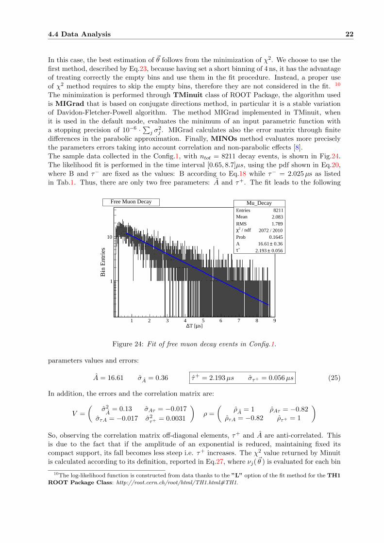
differences in the parabolic approximation. Finally, MINOs method evaluates more preciselythe parameters errors taking into account correlation and non-parabolic effects [8].The sample data collected in the Config.1, with ntot = 8211 decay events, is shown in Fig.24.The likelihood fit is performed in the time interval [0.65, 8.7]µs, using the pdf shown in Eq.20,where B and τ− are fixed as the values: B according to Eq.18 while τ− = 2.025µs as listedin Tab.1. Thus, there are only two free parameters: A and τ+. The fit leads to the following
Mu_DecayEntries 8211Mean 2.083RMS 1.789
/ ndf 2χ 2072 / 2010Prob 0.1645A 0.36± 16.61
+τ 0.056± 2.193
s]µT [∆1 2 3 4 5 6 7 8 9
Bin
Ent
ries
1
10
Mu_DecayEntries 8211Mean 2.083RMS 1.789
/ ndf 2χ 2072 / 2010Prob 0.1645A 0.36± 16.61
+τ 0.056± 2.193
Free Muon Decay
Figure 24: Fit of free muon decay events in Config.1.
parameters values and errors:
A = 16.61 σA = 0.36 τ+ = 2.193µs στ+ = 0.056µs (25)
In addition, the errors and the correlation matrix are:
V =
(σ2A
= 0.13 σAτ = −0.017
στA = −0.017 σ2τ+ = 0.0031
)ρ =
(ρA = 1 ρAτ = −0.82
ρτA = −0.82 ρτ+ = 1
)So, observing the correlation matrix off-diagonal elements, τ+ and A are anti-correlated. Thisis due to the fact that if the amplitude of an exponential is reduced, maintaining fixed itscompact support, its fall becomes less steep i.e. τ+ increases. The χ2 value returned by Minuitis calculated according to its definition, reported in Eq.27, where νj( ~θ ) is evaluated for each bin
10The log-likelihood function is constructed from data thanks to the ”L” option of the fit method for the TH1ROOT Package Class: http://root.cern.ch/root/html/TH1.html#TH1.
4.4 Data Analysis 23
(the empty bins are not skipped) after the minimization process and σ2j = νj( ~θ ). The χ2 value
and its probability, obtained from the fit, are:
χ20 =
χ2
ndf= 1.031 P (χ2 > χ2
0) = 16.45 % ∈ 95%C.L.
However, these results cannot be considered completely reliable, in fact:
• When we consider a sample of a random variable xi, distributed according to the pdff(x, θ ), the maximum likelihood method allows to estimate θ as θ. The estimator θ is itselfa random variable, dependent from xi, distributed according to g( θ, θtrue ). In generalterms, ML estimators are consistent, not biased or asymptotically not biased, robust andg( θ, θtrue ) is approximately Gausssian [9]. The problem is that g( θ, θtrue ) is not known,so if we want a correct estimate for the variance σ2
θwe have to build g( θ, θtrue ) from a
Monte-Carlo simulation.
• The χ2 is a measurement of the global agreement between the data and the hypothesismade about their distribution. In fact, if nj are independent Gausssian variables, and if
the functional hypothesis for νj( ~θ ) is true, the χ2 value, obtained from the minimizationof Eq.27, is distributed according to the χ2 distribution:
f(k = χ2, ndf ) =1
2ndf/2Γ(ndf/2)kndf2−1e−k/2 (26)
Thus, the significance for a given value of χ2 called χ20 is defined as:
P (χ2 > χ20) =
ˆ +∞
χ20
f(k, ndf ) dk (27)
Note that if ndf 1 the χ2 distribution f(k, ndf ) → a Gausssian pdf with mean ndf andvariance 2ndf [9]. In our case, nj are counts so they follow a Poisson distribution thatis substantially different from a Gausssian pdf when nj 6 10. Thus, if we want to usethe χ2 test to check the agreement between data and hypothesis, we have to control if itsdistribution follows what predicted from the theory.
• All minimization algorithms allow the search for local minimum. The only way to checkif we get an absolute one consists of repeating the minimization procedure from differentstarting points in parameter space.
Starting from the experimental data collected in Config.1, a set of Monte-Carlo pseudo-experimentsare developed in order to answer to the previous questions testing the stability and the goodnessof the fit procedure:
1. Let’s assume that the estimators τ+ and A are not-biased, so we use their values reportedin Eq.25 as expected value for τ+ and A in the Monte-Carlo.
2. In each pseudo-experiment, the content of each bin is generated using a Poisson smearingaround a expected value given by: 11
νj(τ+, A) = ntot ·
ˆ tmaxj
tminj
f(t, τ+, A)dt (28)
11The random Poisson generator and the uniform one belongs to the class TRandom3 of ROOT Packagehttp://root.cern.ch/root/htmldoc/TRandom.html#TRandom.
4.4 Data Analysis 24
3. Each generated spectrum is fitted with the likelihood method previously described. Theparameters are initialized using a Monte-Carlo grid around τ+ and A i.e. before each fitthese free parameters are randomly set using a uniform number generator in the intervals[τ+ − 30% · τ+, τ+ + 30% · τ+], [A− 30% · A, A+ 30% · A].
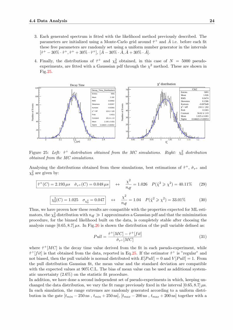
4. Finally, the distributions of τ+ and χ20 obtained, in this case of N = 5000 pseudo-
experiments, are fitted with a Gausssian pdf through the χ2 method. These are shown inFig.25.
Decay_Time_Distribution1
Entries 5001
Mean 2.192
RMS 0.04902
Skewness 0.02467
Kurtosis -0.03361
/ ndf 2χ 123.2 / 120
Prob 0.4011
Constant 1.8± 101.4
Mean 0.001± 2.193
Sigma 0.00053± 0.04824
s]µ [+µτ
2 2.1 2.2 2.3 2.4
Num
ber
of E
vent
s
0
20
40
60
80
100
120Decay_Time_Distribution1
Entries 5001
Mean 2.192
RMS 0.04902
Skewness 0.02467
Kurtosis -0.03361
/ ndf 2χ 123.2 / 120
Prob 0.4011
Constant 1.8± 101.4
Mean 0.001± 2.193
Sigma 0.00053± 0.04824
Decay TimeChi2
Entries 5001Mean 1.026RMS 0.0474Skewness 0.1586Kurtosis -0.007649
/ ndf 2χ 210.3 / 202Prob 0.3301Constant 1.03± 56.62 Mean 0.001± 1.025 Sigma 0.00053± 0.04663
02χ
0.85 0.9 0.95 1 1.05 1.1 1.15 1.2
Num
ber
of E
vent
s
0
10
20
30
40
50
60
70 Chi2Entries 5001Mean 1.026RMS 0.0474Skewness 0.1586Kurtosis -0.007649
/ ndf 2χ 210.3 / 202Prob 0.3301Constant 1.03± 56.62 Mean 0.001± 1.025 Sigma 0.00053± 0.04663
distribution2χ
Figure 25: Left: τ+ distribution obtained from the MC simulations. Right: χ20 distribution
obtained from the MC simulations.
Analysing the distributions obtained from these simulations, best estimations of τ+, στ+ andχ2
0 are given by:
τ+(C) = 2.193µs στ+(C) = 0.048µs ↔ χ2
ndf= 1.026 P (χ2 > χ2) = 40.11% (29)
χ20(C) = 1.025 σχ2
0= 0.047 ↔ χ2
ndf= 1.04 P (χ2 > χ2) = 33.01% (30)
Thus, we have proven how these results are compatible with the properties expected for ML esti-mators, the χ2
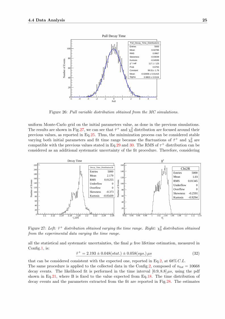
0 distribution with ndf 1 approximates a Gaussian pdf and that the minimizationprocedure, for the binned likelihood built on the data, is completely stable after choosing theanalysis range [0.65, 8.7]µs. In Fig.26 is shown the distribution of the pull variable defined as:
Pull =τ+[MC]− τ+[fit]
στ+ [MC](31)
where τ+[MC] is the decay time value derived from the fit in each pseudo-experiment, whileτ+[fit] is that obtained from the data, reported in Eq.25. If the estimator τ+ is ”regular” andnot biased, then the pull variable is normal distributed with E[Pull] = 0 and V [Pull] = 1. Fromthe pull distribution Gaussian fit, the mean value and the standard deviation are compatiblewith the expected values at 90% C.L. The bias of mean value can be used as additional system-atic uncertainty (2.6%) on the statistic fit procedure.In addition, we have done a second independent set of pseudo-experiments in which, keeping un-changed the data distribution, we vary the fit range previously fixed in the interval [0.65, 8.7]µs.In each simulation, the range extremes are randomly generated according to a uniform distri-bution in the gate [tmin − 250 ns , tmin + 250 ns], [tmax − 200 ns , tmax + 200 ns] together with a
4.4 Data Analysis 25
Pull_Decay_Time_Distribution1
Entries 5000
Mean -0.02785
RMS 0.9967
Skewness -0.03039
Kurtosis -0.04599
/ ndf 2χ 117.1 / 125
Prob 0.6793
Constant 1.76± 99.51
Mean 0.01415± -0.02658
Sigma 0.0104± 0.9803
Pull-5 -4 -3 -2 -1 0 1 2 3 4 5
Num
ber
of E
vent
s
0
20
40
60
80
100
Pull_Decay_Time_Distribution1
Entries 5000
Mean -0.02785
RMS 0.9967
Skewness -0.03039
Kurtosis -0.04599
/ ndf 2χ 117.1 / 125
Prob 0.6793
Constant 1.76± 99.51
Mean 0.01415± -0.02658
Sigma 0.0104± 0.9803
Pull Decay Time
Figure 26: Pull variable distribution obtained from the MC simulations.
uniform Monte-Carlo grid on the initial parameters value, as done in the previous simulations.The results are shown in Fig.27, we can see that τ+ and χ2
0 distribution are focused around theirprevious values, as reported in Eq.25. Thus, the minimization process can be considered stablevarying both initial parameters and fit time range because the fluctuations of τ+ and χ2
0 arecompatible with the previous values stated in Eq.29 and 30. The RMS of τ+ distribution can beconsidered as an additional systematic uncertainty of the fit procedure. Therefore, considering
Decay_Time_Distribution1R
Entries 5000
Mean 2.179
RMS 0.01255
Underflow 0
Overflow 0
Skewness -0.373
Kurtosis -0.05439
s]µ [+µτ
2.1 2.12 2.14 2.16 2.18 2.2 2.22 2.24 2.26
Num
ber
of E
vent
s
0
20
40
60
80
100
120
140
160
180
200
220Decay_Time_Distribution1R
Entries 5000
Mean 2.179
RMS 0.01255
Underflow 0
Overflow 0
Skewness -0.373
Kurtosis -0.05439
Decay Time
Chi2REntries 5000Mean 1.03RMS 0.01345
Underflow 0Overflow 0Skewness -0.2591Kurtosis -0.9294
02χ
0.92 0.94 0.96 0.98 1 1.02 1.04 1.06 1.08 1.1 1.12 1.14
Num
ber
of E
vent
s
0
20
40
60
80
100
120
140
160
Chi2REntries 5000Mean 1.03RMS 0.01345
Underflow 0Overflow 0Skewness -0.2591Kurtosis -0.9294
2χ
Figure 27: Left: τ+ distribution obtained varying the time range. Right: χ20 distribution obtained
from the experimental data varying the time range.
all the statistical and systematic uncertainties, the final µ free lifetime estimation, measured inConfig.1, is:
τ+ = 2.193± 0.048(stat.)± 0.058(sys.)µs (32)
that can be considered consistent with the expected one, reported in Eq.2, at 68%C.L.The same procedure is applied to the collected data in the Config.2, composed of ntot = 10668decay events. The likelihood fit is performed in the time interval [0.9, 8.8]µs, using the pdfshown in Eq.21, where B is fixed to the value expected from Eq.18. The time distribution ofdecay events and the parameters extracted from the fit are reported in Fig.28. The estimates
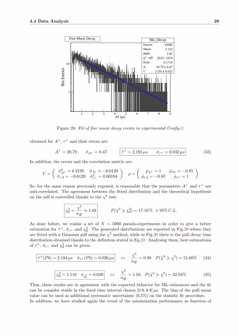
4.4 Data Analysis 26
Mu_DecayEntries 10668Mean 2.132RMS 1.82
/ ndf 2χ 2033 / 1974Prob 0.1719
A 0.47± 20.79 +τ 0.032± 2.191
s]µT [∆1 2 3 4 5 6 7 8 9
Bin
Ent
ries
1
10
Mu_DecayEntries 10668Mean 2.132RMS 1.82
/ ndf 2χ 2033 / 1974Prob 0.1719
A 0.47± 20.79 +τ 0.032± 2.191
Free Muon Decay
Figure 28: Fit of free muon decay events in experimental Config.2.
obtained for A+, τ+ and their errors are:
A+ = 20.79 σA+ = 0.47 τ+ = 2.191µs στ+ = 0.032µs (33)
In addition, the errors and the correlation matrix are:
V =
(σ2A+ = 0.2195 σAτ = −0.0129
στA = −0.0129 σ2τ+ = 0.00104
)ρ =
(ρA+ = 1 ρAτ = −0.85
ρτA = −0.85 ρτ+ = 1
)So, for the same reason previously exposed, is reasonable that the parameters A+ and τ+ areanti-correlated. The agreement between the fitted distribution and the theoretical hypothesison the pdf is controlled thanks to the χ2 test:
χ20 =
χ2
ndf≈ 1.03 P (χ2 > χ2
0) = 17.19 % ∈ 95%C.L.
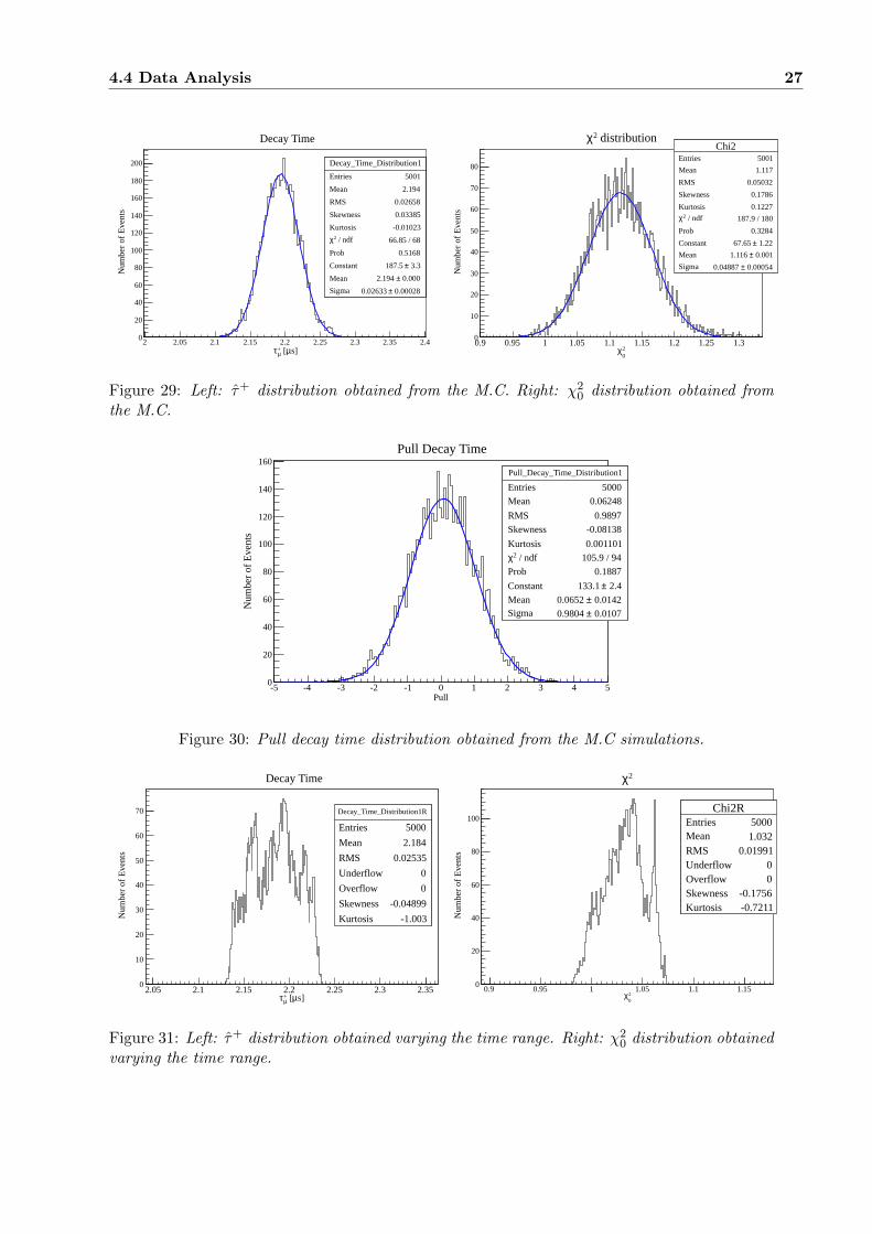
As done before, we realize a set of N = 5000 pseudo-experiments in order to give a betterestimation for τ+, στ+ and χ2
0. The generated distributions are reported in Fig.29 where theyare fitted with a Gaussian pdf using the χ2 method; while in Fig.30 there is the pull decay timedistribution obtained thanks to the definition stated in Eq.31. Analysing them, best estimationsof τ+, στ+ and χ2
0 can be given:
τ+(Pb) = 2.194µs στ+(Pb) = 0.026µs ↔ χ2
ndf= 0.98 P (χ2 > χ2) = 51.68% (34)
χ20 = 1.116 σχ2
0= 0.049 ↔ χ2
ndf= 1.04 P (χ2 > χ2) = 32.84% (35)
Thus, these results are in agreement with the expected behavior for ML estimators and the fitcan be consider stable in the fixed time interval chosen [0.9, 8.8]µs. The bias of the pull meanvalue can be used as additional systematic uncertainty (6.5%) on the statistic fit procedure.In addition, we have studied again the trend of the minimization performance as function of
4.4 Data Analysis 27
Decay_Time_Distribution1
Entries 5001
Mean 2.194
RMS 0.02658
Skewness 0.03385
Kurtosis -0.01023
/ ndf 2χ 66.85 / 68
Prob 0.5168
Constant 3.3± 187.5
Mean 0.000± 2.194
Sigma 0.00028± 0.02633
s]µ [+µτ
2 2.05 2.1 2.15 2.2 2.25 2.3 2.35 2.4
Num
ber
of E
vent
s
0
20
40
60
80
100
120
140
160
180
200 Decay_Time_Distribution1
Entries 5001
Mean 2.194
RMS 0.02658
Skewness 0.03385
Kurtosis -0.01023
/ ndf 2χ 66.85 / 68
Prob 0.5168
Constant 3.3± 187.5
Mean 0.000± 2.194
Sigma 0.00028± 0.02633
Decay TimeChi2
Entries 5001
Mean 1.117
RMS 0.05032
Skewness 0.1786
Kurtosis 0.1227
/ ndf 2χ 187.9 / 180
Prob 0.3284
Constant 1.22± 67.65
Mean 0.001± 1.116
Sigma 0.00054± 0.04887
02χ
0.9 0.95 1 1.05 1.1 1.15 1.2 1.25 1.3
Num
ber
of E
vent
s
0
10
20
30
40
50
60
70
80
Chi2Entries 5001
Mean 1.117
RMS 0.05032
Skewness 0.1786
Kurtosis 0.1227
/ ndf 2χ 187.9 / 180
Prob 0.3284
Constant 1.22± 67.65
Mean 0.001± 1.116
Sigma 0.00054± 0.04887
distribution2χ
Figure 29: Left: τ+ distribution obtained from the M.C. Right: χ20 distribution obtained from
the M.C.
Pull_Decay_Time_Distribution1
Entries 5000
Mean 0.06248
RMS 0.9897
Skewness -0.08138
Kurtosis 0.001101
/ ndf 2χ 105.9 / 94
Prob 0.1887
Constant 2.4± 133.1
Mean 0.0142± 0.0652 Sigma 0.0107± 0.9804
Pull-5 -4 -3 -2 -1 0 1 2 3 4 5
Num
ber
of E
vent
s
0
20
40
60
80
100
120
140
160Pull_Decay_Time_Distribution1
Entries 5000
Mean 0.06248
RMS 0.9897
Skewness -0.08138
Kurtosis 0.001101
/ ndf 2χ 105.9 / 94
Prob 0.1887
Constant 2.4± 133.1
Mean 0.0142± 0.0652 Sigma 0.0107± 0.9804
Pull Decay Time
Figure 30: Pull decay time distribution obtained from the M.C simulations.
Decay_Time_Distribution1R
Entries 5000
Mean 2.184
RMS 0.02535
Underflow 0
Overflow 0
Skewness -0.04899
Kurtosis -1.003
s]µ [+µτ
2.05 2.1 2.15 2.2 2.25 2.3 2.35
Num
ber
of E
vent
s
0
10
20
30
40
50
60
70 Decay_Time_Distribution1R
Entries 5000
Mean 2.184
RMS 0.02535
Underflow 0
Overflow 0
Skewness -0.04899
Kurtosis -1.003
Decay Time
Chi2REntries 5000Mean 1.032RMS 0.01991Underflow 0Overflow 0Skewness -0.1756Kurtosis -0.7211
02χ
0.9 0.95 1 1.05 1.1 1.15
Num
ber
of E
vent
s
0
20
40
60
80
100Chi2R
Entries 5000Mean 1.032RMS 0.01991Underflow 0Overflow 0Skewness -0.1756Kurtosis -0.7211
2χ
Figure 31: Left: τ+ distribution obtained varying the time range. Right: χ20 distribution obtained
varying the time range.
4.5 Muon lifetime in Aluminium 28
the time range. So, other 10000 simulations are performed changing any time the fit extremesgenerating them uniformly in the intervals [tmin−500ns, tmin+500ns] and [tmax−200ns, tmax+200ns]. The results consist of the τ+ and the χ2
0 distributions shown in Fig.31. Therefore, theminimization process can be considered stable varying both initial parameters and fit time rangebecause the fluctuations of τ+ and χ2
0 are compatible with the measured value reported in Eq.34and 35. The RMS of τ+ distribution can be considered as an additional systematic uncertaintyof the fit procedure. Therefore, considering all the statistical and systematic uncertainties, thefinal µ free lifetime estimation, measured in Config.2, is:
τ+ = 2.194± 0.026(stat.)± 0.145(sys.)µs (36)
that can be considered consistent with the expected one, reported in Eq.2, at 68%C.L.
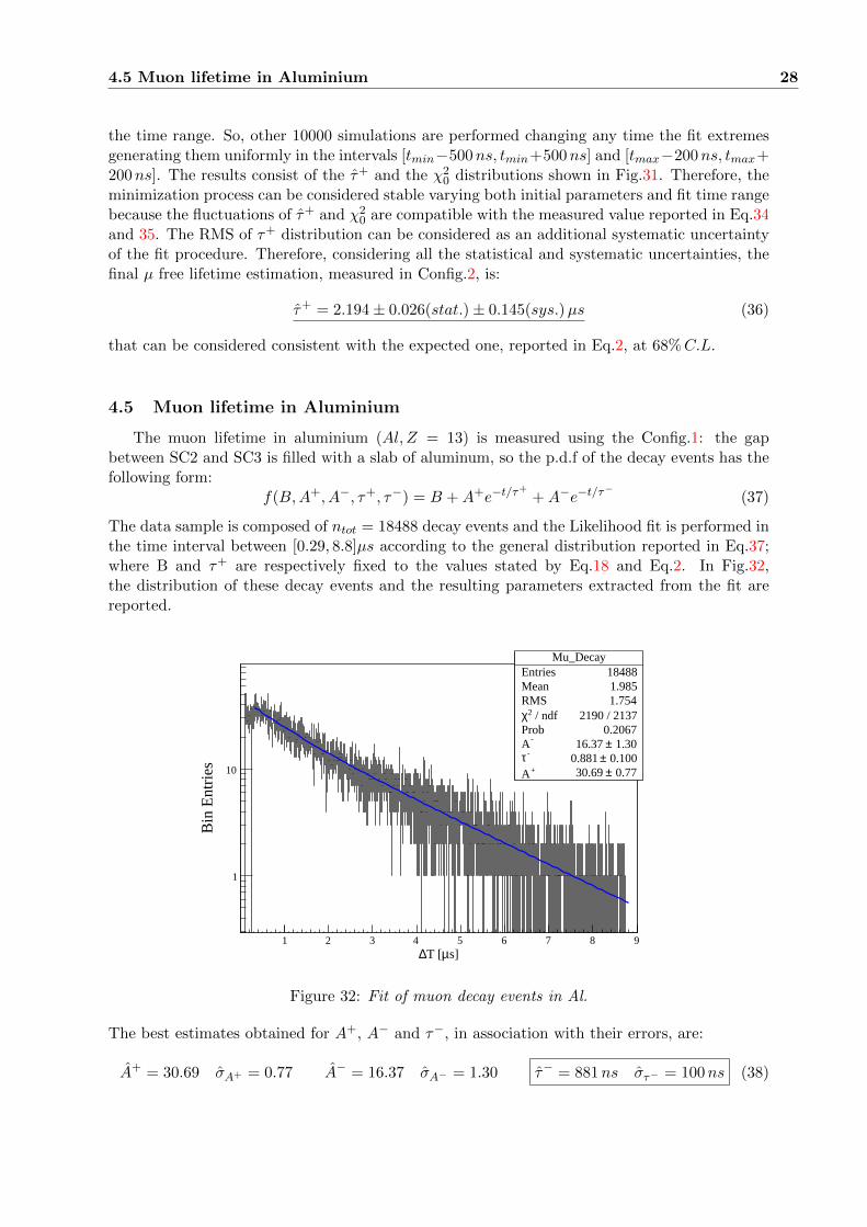
4.5 Muon lifetime in Aluminium
The muon lifetime in aluminium (Al, Z = 13) is measured using the Config.1: the gapbetween SC2 and SC3 is filled with a slab of aluminum, so the p.d.f of the decay events has thefollowing form:
f(B,A+, A−, τ+, τ−) = B +A+e−t/τ+
+A−e−t/τ−
(37)
The data sample is composed of ntot = 18488 decay events and the Likelihood fit is performed inthe time interval between [0.29, 8.8]µs according to the general distribution reported in Eq.37;where B and τ+ are respectively fixed to the values stated by Eq.18 and Eq.2. In Fig.32,the distribution of these decay events and the resulting parameters extracted from the fit arereported.
Mu_DecayEntries 18488Mean 1.985RMS 1.754
/ ndf 2χ 2190 / 2137Prob 0.2067
-A 1.30± 16.37 -τ 0.100± 0.881 +A 0.77± 30.69
s]µT [∆1 2 3 4 5 6 7 8 9
Bin
Ent
ries
1
10
Mu_DecayEntries 18488Mean 1.985RMS 1.754
/ ndf 2χ 2190 / 2137Prob 0.2067
-A 1.30± 16.37 -τ 0.100± 0.881 +A 0.77± 30.69
Figure 32: Fit of muon decay events in Al.
The best estimates obtained for A+, A− and τ−, in association with their errors, are:
A+ = 30.69 σA+ = 0.77 A− = 16.37 σA− = 1.30 τ− = 881ns στ− = 100ns (38)
4.5 Muon lifetime in Aluminium 29
In addition, the errors and the correlation matrix are:
V =
σ2A− = 1.709 σA−τ = −0.062 σA−A+ = −0.021
στA− = −0.062 σ2τ− = 0.01 στA+ = −0.0625
σA+A− = −0.021 σA+τ = −0.625 σ2A+ = 0.591
ρ =
ρA− = 1 ρA−τ = −0.475 ρA−A+ = −0.021ρτA− = −0.475 ρτ−µ = 1 ρτA+ = −0.811
ρA+A− = −0.021 ρA+τ = −0.811 ρA+ = 1
The agreement between the fitted distribution and the theoretical hypothesis on the pdf ischecked through the χ2 test:
χ20 =
χ2
ndf≈ 1.025 P (χ2 > χ2
0) = 20.67 % ∈ 95%C.L.
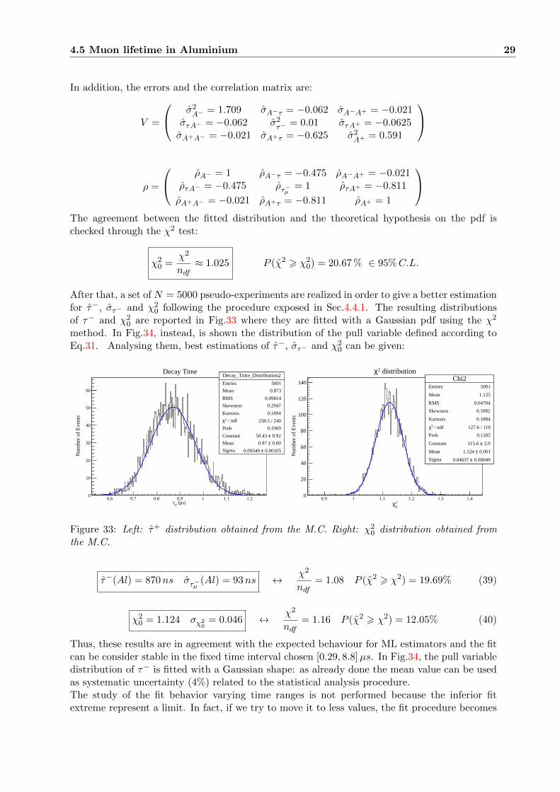
After that, a set of N = 5000 pseudo-experiments are realized in order to give a better estimationfor τ−, στ− and χ2
0 following the procedure exposed in Sec.4.4.1. The resulting distributionsof τ− and χ2
0 are reported in Fig.33 where they are fitted with a Gaussian pdf using the χ2
method. In Fig.34, instead, is shown the distribution of the pull variable defined according toEq.31. Analysing them, best estimations of τ−, στ− and χ2
0 can be given:
Decay_Time_Distribution2
Entries 5001
Mean 0.873
RMS 0.09814
Skewness 0.2947
Kurtosis 0.1894
/ ndf 2χ 258.5 / 240
Prob 0.1969
Constant 0.92± 50.43
Mean 0.00± 0.87
Sigma 0.00105± 0.09349
s]µ [-µτ
0.6 0.7 0.8 0.9 1 1.1 1.2
Num
ber
of E
vent
s
0
10
20
30
40
50
60
Decay_Time_Distribution2
Entries 5001
Mean 0.873
RMS 0.09814
Skewness 0.2947
Kurtosis 0.1894
/ ndf 2χ 258.5 / 240
Prob 0.1969
Constant 0.92± 50.43
Mean 0.00± 0.87
Sigma 0.00105± 0.09349
Decay TimeChi2
Entries 5001
Mean 1.125
RMS 0.04704
Skewness 0.1082
Kurtosis 0.1084
/ ndf 2χ 127.6 / 110
Prob 0.1205
Constant 2.0± 115.6
Mean 0.001± 1.124
Sigma 0.00049± 0.04637
02χ
0.9 1 1.1 1.2 1.3 1.4
Num
ber
of E
vent
s
0
20
40
60
80
100
120
140Chi2
Entries 5001
Mean 1.125
RMS 0.04704
Skewness 0.1082
Kurtosis 0.1084
/ ndf 2χ 127.6 / 110
Prob 0.1205
Constant 2.0± 115.6
Mean 0.001± 1.124
Sigma 0.00049± 0.04637
distribution2χ
Figure 33: Left: τ+ distribution obtained from the M.C. Right: χ20 distribution obtained from
the M.C.
τ−(Al) = 870ns στ−µ (Al) = 93ns ↔ χ2
ndf= 1.08 P (χ2 > χ2) = 19.69% (39)
χ20 = 1.124 σχ2
0= 0.046 ↔ χ2
ndf= 1.16 P (χ2 > χ2) = 12.05% (40)
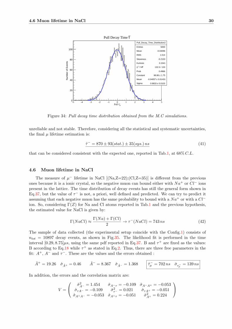
Thus, these results are in agreement with the expected behaviour for ML estimators and the fitcan be consider stable in the fixed time interval chosen [0.29, 8.8]µs. In Fig.34, the pull variabledistribution of τ− is fitted with a Gaussian shape: as already done the mean value can be usedas systematic uncertainty (4%) related to the statistical analysis procedure.The study of the fit behavior varying time ranges is not performed because the inferior fitextreme represent a limit. In fact, if we try to move it to less values, the fit procedure becomes
4.6 Muon lifetime in NaCl 30
Pull_Decay_Time_Distribution2
Entries 5000
Mean -0.04096
RMS 1.014
Skewness -0.2103
Kurtosis 0.1541
/ ndf 2χ 132.5 / 133
Prob 0.4966
Constant 1.75± 98.86
Mean 0.01431± -0.04057
Sigma 0.0103± 0.9833
-µτPull
-5 -4 -3 -2 -1 0 1 2 3 4 5
Num
ber
of E
vent
s
0
20
40
60
80
100
Pull_Decay_Time_Distribution2
Entries 5000
Mean -0.04096
RMS 1.014
Skewness -0.2103
Kurtosis 0.1541
/ ndf 2χ 132.5 / 133
Prob 0.4966
Constant 1.75± 98.86
Mean 0.01431± -0.04057
Sigma 0.0103± 0.9833
-τPull Decay Time
Figure 34: Pull decay time distribution obtained from the M.C simulations.
unreliable and not stable. Therefore, considering all the statistical and systematic uncertainties,the final µ lifetime estimation is:
τ− = 870± 93(stat.)± 35(sys.)ns (41)
that can be considered consistent with the expected one, reported in Tab.1, at 68%C.L.
4.6 Muon lifetime in NaCl
The measure of µ− lifetime in NaCl [(Na,Z=22);(Cl,Z=35)] is different from the previousones because it is a ionic crystal, so the negative muon can bound either with Na+ or Cl− ionspresent in the lattice. The time distribution of decay events has still the general form shown inEq.37, but the value of τ− is not, a priori, well defined and predicted. We can try to predict itassuming that each negative muon has the same probability to bound with a Na+ or with a Cl−
ion. So, considering Γ(Z) for Na and Cl atoms reported in Tab.1 and the previous hypothesis,the estimated value for NaCl is given by:
Γ(NaCl) ≈ Γ(Na) + Γ(Cl)
2→ τ−(NaCl) = 743ns (42)
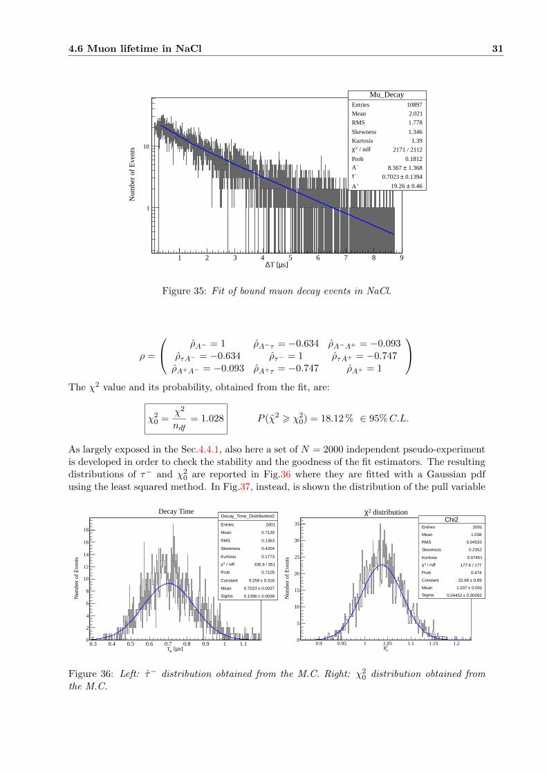
The sample of data collected (the experimental setup coincide with the Config.1) consists ofntot = 10897 decay events, as shown in Fig.35. The likelihood fit is performed in the timeinterval [0.29, 8.75]µs, using the same pdf reported in Eq.37. B and τ+ are fixed as the values:B according to Eq.18 while τ+ as stated in Eq.2. Thus, there are three free parameters in thefit: A+, A− and τ−. These are the values and the errors obtained :
A+ = 19.26 σA+ = 0.46 A− = 8.367 σA− = 1.368 τ−µ = 702ns στ−µ = 139ns
In addition, the errors and the correlation matrix are:
V =
σ2A− = 1.454 σA−τ = −0.109 σA−A+ = −0.053
στA− = −0.109 σ2τ− = 0.021 στA+ = −0.051
σA+A− = −0.053 σA+τ = −0.051 σ2A+ = 0.224
4.6 Muon lifetime in NaCl 31
Mu_DecayEntries 10897
Mean 2.021
RMS 1.778
Skewness 1.346
Kurtosis 1.39 / ndf 2χ 2171 / 2112
Prob 0.1812 -A 1.368± 8.367
-τ 0.1394± 0.7023
+A 0.46± 19.26
s]µT [∆1 2 3 4 5 6 7 8 9
Num
ber
of E
vent
s
1
10
Mu_DecayEntries 10897
Mean 2.021
RMS 1.778
Skewness 1.346
Kurtosis 1.39 / ndf 2χ 2171 / 2112
Prob 0.1812 -A 1.368± 8.367
-τ 0.1394± 0.7023
+A 0.46± 19.26
Figure 35: Fit of bound muon decay events in NaCl.
ρ =
ρA− = 1 ρA−τ = −0.634 ρA−A+ = −0.093ρτA− = −0.634 ρτ− = 1 ρτA+ = −0.747ρA+A− = −0.093 ρA+τ = −0.747 ρA+ = 1
The χ2 value and its probability, obtained from the fit, are:
χ20 =
χ2
ndf= 1.028 P (χ2 > χ2
0) = 18.12 % ∈ 95%C.L.
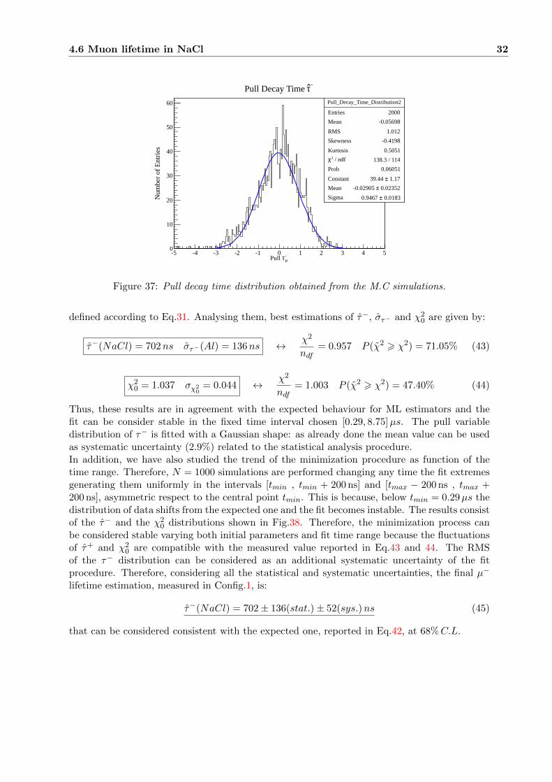
As largely exposed in the Sec.4.4.1, also here a set of N = 2000 independent pseudo-experimentis developed in order to check the stability and the goodness of the fit estimators. The resultingdistributions of τ− and χ2
0 are reported in Fig.36 where they are fitted with a Gaussian pdfusing the least squared method. In Fig.37, instead, is shown the distribution of the pull variable
Decay_Time_Distribution2
Entries 2001
Mean 0.7139
RMS 0.1363
Skewness 0.4204
Kurtosis 0.1773
/ ndf 2χ 335.9 / 351
Prob 0.7105
Constant 0.316± 9.259
Mean 0.0037± 0.7023
Sigma 0.0038± 0.1356
s]µ [-µτ
0.3 0.4 0.5 0.6 0.7 0.8 0.9 1 1.1
Num
ber
of E
vent
s
0
2
4
6
8
10
12
14
16
18
Decay_Time_Distribution2
Entries 2001
Mean 0.7139
RMS 0.1363
Skewness 0.4204
Kurtosis 0.1773
/ ndf 2χ 335.9 / 351
Prob 0.7105
Constant 0.316± 9.259
Mean 0.0037± 0.7023
Sigma 0.0038± 0.1356
Decay TimeChi2
Entries 2001
Mean 1.038
RMS 0.04533
Skewness 0.2352
Kurtosis 0.07451
/ ndf 2χ 177.6 / 177
Prob 0.474
Constant 0.69± 22.66
Mean 0.001± 1.037
Sigma 0.00092± 0.04452
02χ
0.9 0.95 1 1.05 1.1 1.15 1.2
Num
ber
of E
vent
s
0
5
10
15
20
25
30
35Chi2
Entries 2001
Mean 1.038
RMS 0.04533
Skewness 0.2352
Kurtosis 0.07451
/ ndf 2χ 177.6 / 177
Prob 0.474
Constant 0.69± 22.66
Mean 0.001± 1.037
Sigma 0.00092± 0.04452
distribution2χ
Figure 36: Left: τ− distribution obtained from the M.C. Right: χ20 distribution obtained from
the M.C.
4.6 Muon lifetime in NaCl 32
Pull_Decay_Time_Distribution2
Entries 2000
Mean -0.05698
RMS 1.012
Skewness -0.4198
Kurtosis 0.5051
/ ndf 2χ 138.3 / 114
Prob 0.06051
Constant 1.17± 39.44
Mean 0.02352± -0.02905
Sigma 0.0183± 0.9467
-µτPull
-5 -4 -3 -2 -1 0 1 2 3 4 5
Num
ber
of E
ntri
es
0
10
20
30
40
50
60 Pull_Decay_Time_Distribution2
Entries 2000
Mean -0.05698
RMS 1.012
Skewness -0.4198
Kurtosis 0.5051
/ ndf 2χ 138.3 / 114
Prob 0.06051
Constant 1.17± 39.44
Mean 0.02352± -0.02905
Sigma 0.0183± 0.9467
-τPull Decay Time
Figure 37: Pull decay time distribution obtained from the M.C simulations.
defined according to Eq.31. Analysing them, best estimations of τ−, στ− and χ20 are given by:
τ−(NaCl) = 702ns στ−(Al) = 136ns ↔ χ2
ndf= 0.957 P (χ2 > χ2) = 71.05% (43)
χ20 = 1.037 σχ2
0= 0.044 ↔ χ2
ndf= 1.003 P (χ2 > χ2) = 47.40% (44)
Thus, these results are in agreement with the expected behaviour for ML estimators and thefit can be consider stable in the fixed time interval chosen [0.29, 8.75]µs. The pull variabledistribution of τ− is fitted with a Gaussian shape: as already done the mean value can be usedas systematic uncertainty (2.9%) related to the statistical analysis procedure.In addition, we have also studied the trend of the minimization procedure as function of thetime range. Therefore, N = 1000 simulations are performed changing any time the fit extremesgenerating them uniformly in the intervals [tmin , tmin + 200 ns] and [tmax − 200 ns , tmax +200 ns], asymmetric respect to the central point tmin. This is because, below tmin = 0.29µs thedistribution of data shifts from the expected one and the fit becomes instable. The results consistof the τ− and the χ2
0 distributions shown in Fig.38. Therefore, the minimization process canbe considered stable varying both initial parameters and fit time range because the fluctuationsof τ+ and χ2
0 are compatible with the measured value reported in Eq.43 and 44. The RMSof the τ− distribution can be considered as an additional systematic uncertainty of the fitprocedure. Therefore, considering all the statistical and systematic uncertainties, the final µ−
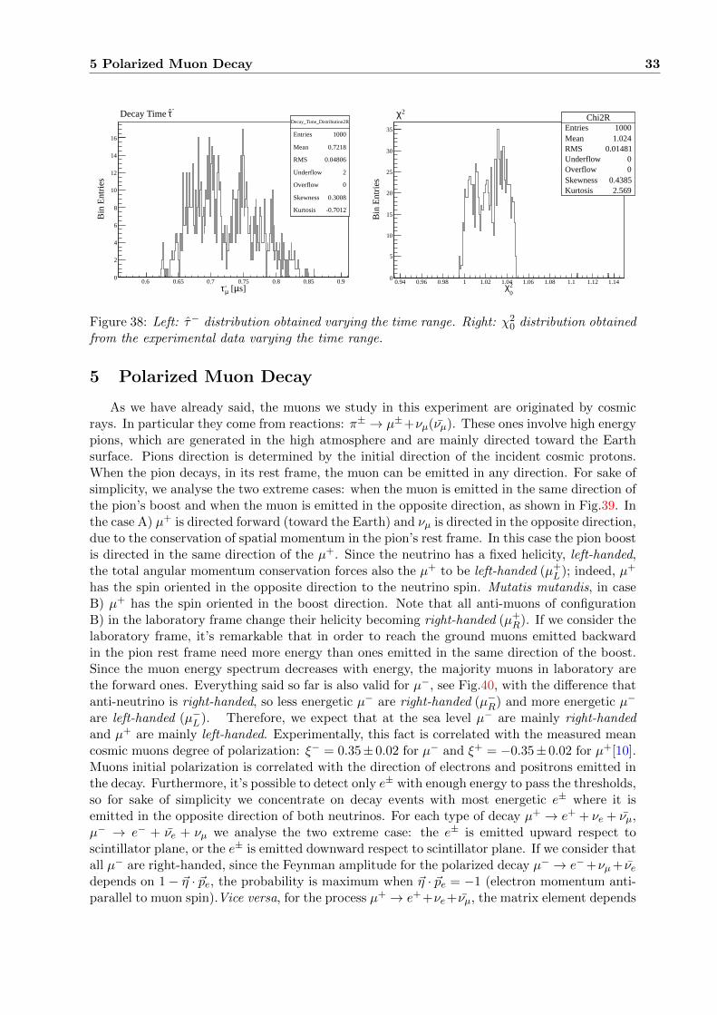
lifetime estimation, measured in Config.1, is:
τ−(NaCl) = 702± 136(stat.)± 52(sys.)ns (45)
that can be considered consistent with the expected one, reported in Eq.42, at 68%C.L.
5 Polarized Muon Decay 33
Decay_Time_Distribution2R
Entries 1000
Mean 0.7218
RMS 0.04806
Underflow 2
Overflow 0
Skewness 0.3008
Kurtosis -0.7012
s]µ [-µτ
0.6 0.65 0.7 0.75 0.8 0.85 0.9
Bin
Ent
ries
0
2
4
6
8
10
12
14
16
Decay_Time_Distribution2R
Entries 1000
Mean 0.7218
RMS 0.04806
Underflow 2
Overflow 0
Skewness 0.3008
Kurtosis -0.7012
-τ Decay Time Chi2REntries 1000Mean 1.024RMS 0.01481Underflow 0Overflow 0Skewness 0.4385Kurtosis 2.569
02χ
0.94 0.96 0.98 1 1.02 1.04 1.06 1.08 1.1 1.12 1.14
Bin
Ent
ries
0
5
10
15
20
25
30
35
Chi2REntries 1000Mean 1.024RMS 0.01481Underflow 0Overflow 0Skewness 0.4385Kurtosis 2.569
2χ
Figure 38: Left: τ− distribution obtained varying the time range. Right: χ20 distribution obtained
from the experimental data varying the time range.
5 Polarized Muon Decay
As we have already said, the muons we study in this experiment are originated by cosmicrays. In particular they come from reactions: π± → µ±+νµ(νµ). These ones involve high energypions, which are generated in the high atmosphere and are mainly directed toward the Earthsurface. Pions direction is determined by the initial direction of the incident cosmic protons.When the pion decays, in its rest frame, the muon can be emitted in any direction. For sake ofsimplicity, we analyse the two extreme cases: when the muon is emitted in the same direction ofthe pion’s boost and when the muon is emitted in the opposite direction, as shown in Fig.39. Inthe case A) µ+ is directed forward (toward the Earth) and νµ is directed in the opposite direction,due to the conservation of spatial momentum in the pion’s rest frame. In this case the pion boostis directed in the same direction of the µ+. Since the neutrino has a fixed helicity, left-handed,the total angular momentum conservation forces also the µ+ to be left-handed (µ+
L ); indeed, µ+
has the spin oriented in the opposite direction to the neutrino spin. Mutatis mutandis, in caseB) µ+ has the spin oriented in the boost direction. Note that all anti-muons of configurationB) in the laboratory frame change their helicity becoming right-handed (µ+
R). If we consider thelaboratory frame, it’s remarkable that in order to reach the ground muons emitted backwardin the pion rest frame need more energy than ones emitted in the same direction of the boost.Since the muon energy spectrum decreases with energy, the majority muons in laboratory arethe forward ones. Everything said so far is also valid for µ−, see Fig.40, with the difference thatanti-neutrino is right-handed, so less energetic µ− are right-handed (µ−R) and more energetic µ−
are left-handed (µ−L ). Therefore, we expect that at the sea level µ− are mainly right-handedand µ+ are mainly left-handed. Experimentally, this fact is correlated with the measured meancosmic muons degree of polarization: ξ− = 0.35± 0.02 for µ− and ξ+ = −0.35± 0.02 for µ+[10].Muons initial polarization is correlated with the direction of electrons and positrons emitted inthe decay. Furthermore, it’s possible to detect only e± with enough energy to pass the thresholds,so for sake of simplicity we concentrate on decay events with most energetic e± where it isemitted in the opposite direction of both neutrinos. For each type of decay µ+ → e+ + νe + νµ,µ− → e− + νe + νµ we analyse the two extreme case: the e± is emitted upward respect toscintillator plane, or the e± is emitted downward respect to scintillator plane. If we consider thatall µ− are right-handed, since the Feynman amplitude for the polarized decay µ− → e−+νµ+ νedepends on 1− ~η · ~pe, the probability is maximum when ~η · ~pe = −1 (electron momentum anti-parallel to muon spin).Vice versa, for the process µ+ → e+ +νe+ νµ, the matrix element depends
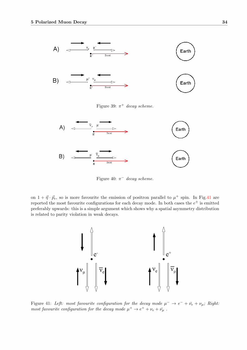
5 Polarized Muon Decay 34
Figure 39: π+ decay scheme.
Figure 40: π− decay scheme.
on 1 + ~η · ~pe, so is more favourite the emission of positron parallel to µ+ spin. In Fig.41 arereported the most favourite configurations for each decay mode. In both cases the e± is emittedpreferably upwards: this is a simple argument which shows why a spatial asymmetry distributionis related to parity violation in weak decays.
Figure 41: Left: most favourite configuration for the decay mode µ− → e− + νe + νµ; Right:most favourite configuration for the decay mode µ+ → e+ + νe + νµ .
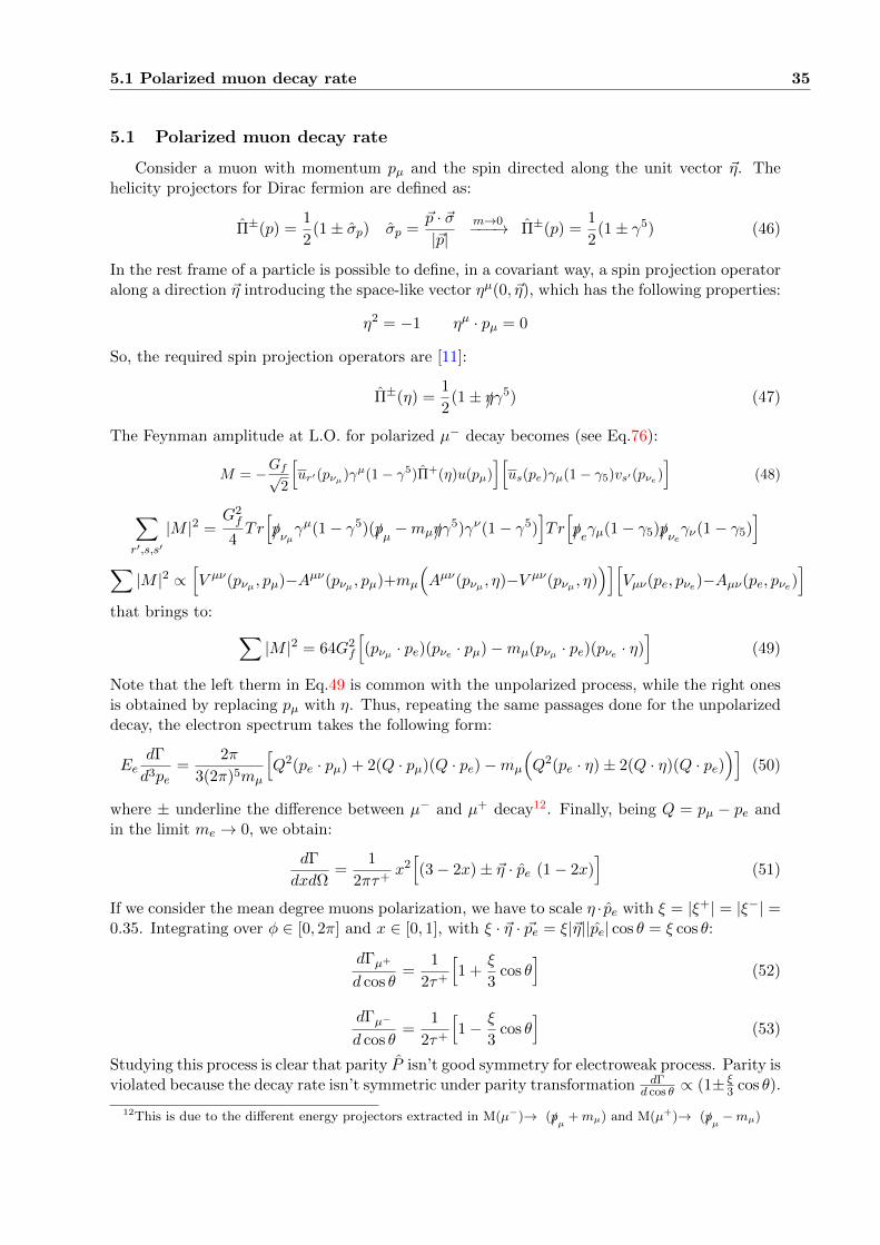
5.1 Polarized muon decay rate 35
5.1 Polarized muon decay rate
Consider a muon with momentum pµ and the spin directed along the unit vector ~η. Thehelicity projectors for Dirac fermion are defined as:
Π±(p) =1
2(1± σp) σp =
~p · ~σ|~p|
m→0−−−→ Π±(p) =1
2(1± γ5) (46)
In the rest frame of a particle is possible to define, in a covariant way, a spin projection operatoralong a direction ~η introducing the space-like vector ηµ(0, ~η), which has the following properties:
η2 = −1 ηµ · pµ = 0
So, the required spin projection operators are [11]:
Π±(η) =1
2(1± /ηγ5) (47)
The Feynman amplitude at L.O. for polarized µ− decay becomes (see Eq.76):
M = −Gf√2
[ur′(pνµ)γµ(1− γ5)Π+(η)u(pµ)
][us(pe)γµ(1− γ5)vs′(pνe)
](48)
∑r′,s,s′
|M |2 =G2f
4Tr[/pνµ
γµ(1− γ5)(/pµ −mµ/ηγ5)γν(1− γ5)
]Tr[/peγµ(1− γ5)/pνe
γν(1− γ5)]
∑|M |2 ∝
[V µν(pνµ , pµ)−Aµν(pνµ , pµ)+mµ
(Aµν(pνµ , η)−V µν(pνµ , η)
)][Vµν(pe, pνe)−Aµν(pe, pνe)
]that brings to: ∑
|M |2 = 64G2f
[(pνµ · pe)(pνe · pµ)−mµ(pνµ · pe)(pνe · η)
](49)
Note that the left therm in Eq.49 is common with the unpolarized process, while the right onesis obtained by replacing pµ with η. Thus, repeating the same passages done for the unpolarizeddecay, the electron spectrum takes the following form:
EedΓ
d3pe=
2π
3(2π)5mµ
[Q2(pe · pµ) + 2(Q · pµ)(Q · pe)−mµ
(Q2(pe · η)± 2(Q · η)(Q · pe)
)](50)
where ± underline the difference between µ− and µ+ decay12. Finally, being Q = pµ − pe andin the limit me → 0, we obtain:
dΓ
dxdΩ=
1
2πτ+x2[(3− 2x)± ~η · pe (1− 2x)
](51)
If we consider the mean degree muons polarization, we have to scale η · pe with ξ = |ξ+| = |ξ−| =0.35. Integrating over φ ∈ [0, 2π] and x ∈ [0, 1], with ξ · ~η · ~pe = ξ|~η||pe| cos θ = ξ cos θ:
dΓµ+
d cos θ=
1
2τ+
[1 +
ξ
3cos θ
](52)
dΓµ−
d cos θ=
1
2τ+
[1− ξ
3cos θ
](53)
Studying this process is clear that parity P isn’t good symmetry for electroweak process. Parity isviolated because the decay rate isn’t symmetric under parity transformation dΓ
d cos θ ∝ (1± ξ3 cos θ).
12This is due to the different energy projectors extracted in M(µ−)→ (/pµ +mµ) and M(µ+)→ (/pµ −mµ)

5.2 Interaction with a Magnetic Field 36
5.2 Interaction with a Magnetic Field
The simple way to align the muon spin along a chosen direction is to exploit the interactionbetween the muon magnetic dipole momentum and an external magnetic field ~B. In QuantumMechanics the Hamiltonian of a free charged particle, with spin S and orbital angular momentumL, in interaction with a E-M field is given by:
H =(p− qA)2
2m+ qφ− ~µS · ~B
~∇· ~A=0, ~B=B0n−−−−−−−−−−→ H = H0 + Hint =p2
2m− (~µL + ~µS) · ~B (54)
where ~µS is given by:
~µS =e
2mcgs ~S
The stationary Schrodinger equation in a uniform magnetic field (to simplify we assume ~B =B0 k), can be easily solved applying the “asymmetric choice”[12], thus the solution consistsof a linear harmonic oscillator along the transverse plane, respect to the direction of ~B, withfrequency:
ω =eB0
mµc(55)
The result of this coupling is the precession of the muon spin ~S around the direction of themagnetic field k, with frequency ω.
5.3 Muon Decay in a Uniform Magnetic Field
If we want to calculate the muon decay rate in a uniform magnetic field, remembering whatwas said in Sec.5.2, we have to correct the spin projection operator in Eq.47 with the precessioneffect:
Π±(η) =1
2[1± /ηγ5 cosωt] (56)
Repeating the same procedure exposed in Sec.5.1, we obtain:
dΓµ+
d cos θ=
1
2τ+
[1 +
ξ
3cos θ cosωt
](57)
dΓµ−
d cos θ=
1
2τ+
[1− ξ
3cos θ cosωt
](58)
Because of the different polarization between positive and negative muons, events with electronemitted in the upper hemisphere (up-events) are obtained for µ+ integrating in Eq.57 cos θ ∈[0, 1] and down events integrating in Eq.57 cos θ ∈ [−1, 0]; on the other hand, for µ− up-events areobtained integrating in Eq.58 cos θ ∈ [−1, 0] and down-events integrating in Eq.58 cos θ ∈ [0, 1]:
Γ(t)upµ+
=1
2τ+
[1 +
ξ
6cosωt
]Γ(t)downµ+ =
1
2τ+
[1− ξ
6cosωt
]Γ(t)up
µ− =1
2τ+
[1 +
ξ
6cosωt
]Γ(t)downµ− =
1
2τ+
[1− ξ
6cosωt
]Note that there’s no difference between Γµ+ and Γµ− .
Γtot = Γup + Γdown =
ˆ 4π
0
1
4πτ+
[1± ξ
3cos θ cosωt
]dΩ =
1
τ+(59)
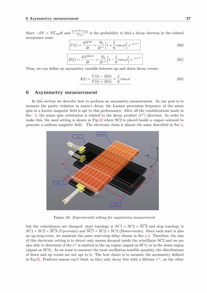
6 Asymmetry measurement 37
Since −dN = NΓtotdt and Γup/down(t)Γtot
is the probability to find a decay electron in the relatedacceptance zone:
U(t) =dNup
dt=
N0
2τ+
[1 +
ξ
6cosωt
]e−t/τ
+(60)
D(t) =dNdown
dt=
N0
2τ+
[1− ξ
6cosωt
]e−t/τ
+(61)
Thus, we can define an asymmetry variable between up and down decay events:
A(t) =U(t)−D(t)
U(t) +D(t)=ξ
6cosωt (62)
6 Asymmetry measurement
In this section we describe how to perform an asymmetry measurement. As our goal is tomeasure the parity violation in muon’s decay, the Larmor precession frequency of the muonspin in a known magnetic field is apt to this performance. After all the considerations made inSec. 5, the muon spin orientation is related to the decay product (e±) direction. In order tomake this, the used setting is shown in Fig.42 where SC2 is placed inside a copper solenoid togenerate a uniform magnetic field. The electronic chain is almost the same described in Sec.4,
Figure 42: Experimental setting for asymmetry measurement.
but the coincidences are changed: start topology is SC1 × SC2 × SC3 and stop topology isSC1× SC2× SC3 (Up-events) and SC1× SC2× SC3 (Down-events). Since each start is alsoan up-stop-event, we maintain the same start-stop delay chosen in Sec.4.2. Therefore, the aimof this electronic setting is to detect only muons decayed inside the scintillator SC2 and we arealso able to determine if the e± is emitted in the up region (signal on SC1) or in the down region(signal on SC3). As we want to measure the most oscillation-sensible quantity, the distributionsof down and up events are not apt to it. The best choice is to measure the asymmetry definedin Eq.62. Positives muons can’t bind, so they only decay free with a lifetime τ+, on the other
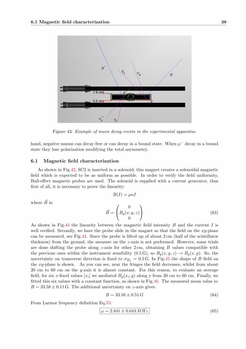
6.1 Magnetic field characterization 38
Figure 43: Example of muon decay events in the experimental apparatus.
hand, negative muons can decay free or can decay in a bound state. When µ− decay in a boundstate they lose polarization modifying the total asymmetry.
6.1 Magnetic field characterization
As shown in Fig.42, SC2 is inserted in a solenoid; this magnet creates a solenoidal magneticfield which is expected to be as uniform as possible. In order to verify the field uniformity,Hall-effect magnetic probes are used. The solenoid is supplied with a current generator, thusfirst of all, it is necessary to prove the linearity:
B(I) = µnI
where ~B is:
~B =
0By(x, y, z)
0
(63)
As shown in Fig.44 the linearity between the magnetic field intensity B and the current I iswell verified. Secondly, we have the probe slide in the magnet so that the field on the xy-planecan be measured, see Fig.42. Since the probe is lifted up of about 2 cm (half of the scintillatorthickness) from the ground, the measure on the z-axis is not performed. However, some trialsare done shifting the probe along z-axis for other 2 cm, obtaining B values compatible withthe previous ones within the instrument sensibility (0.5 G), so By(x, y, z) → By(x, y). So, theuncertainty on transverse direction is fixed to σBx = 0.5 G. In Fig.45 the shape of B field onthe xy-plane is shown. As you can see, near the fringes the field decreases, whilst from about20 cm to 60 cm on the y-axis it is almost constant. For this reason, to evaluate an averagefield, for six x-fixed values [xi] we mediated By(xi, y) along y from 20 cm to 60 cm. Finally, wefitted this six values with a constant function, as shown in Fig.46. The measured mean value is:B = 33.58± 0.11 G. The additional uncertainty on z-axis gives:
B = 33.58± 0.51G (64)
From Larmor frequency definition Eq.55:
ω = 2.841± 0.043MHz (65)
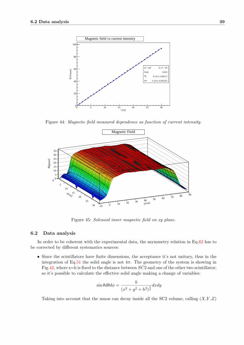
6.2 Data analysis 39
I [A]0 5 10 15 20 25 30
B [
Gau
ss]
0
20
40
60
80
100
/ ndf 2χ 21.17 / 28
Prob 0.818
0B 0.08173± 0.155
n µ 0.005263± 3.124
/ ndf 2χ 21.17 / 28
Prob 0.818
0B 0.08173± 0.155
n µ 0.005263± 3.124
Magnetic field vs current intensity
Figure 44: Magnetic field measured dependence as function of current intensity.
x[cm]
0
5
10
15
20
25
30y[cm]
-10 0 10 20 30 40 50 60 70 80 90
B[g
auss
]
0
5
10
15
20
25
30
35
Magnetic Field
Figure 45: Solenoid inner magnetic field on xy plane.
6.2 Data analysis
In order to be coherent with the experimental data, the asymmetry relation in Eq.62 has tobe corrected by different systematics sources:
• Since the scintillators have finite dimensions, the acceptance it’s not unitary, thus in theintegration of Eq.51 the solid angle is not 4π. The geometry of the system is showing inFig.42, where z=h is fixed to the distance between SC2 and one of the other two scintillator;so it’s possible to calculate the effective solid angle making a change of variables:
sin θdθdφ =h
(x2 + y2 + h2)32
dxdy
Taking into account that the muon can decay inside all the SC2 volume, calling (X,Y ,Z)

6.2 Data analysis 40
x[cm]0 5 10 15 20 25 30
B[g
auss
]
29
30
31
32
33
34
35
36 / ndf 2χ 2.647 / 5
Prob 0.7542
B 0.1078± 33.58
/ ndf 2χ 2.647 / 5
Prob 0.7542
B 0.1078± 33.58
Magnetic Field in 20cm-60cm zone
Figure 46: Average magnetic field in the solenoid.
the muon position in SC2 and d its thickness:
sin θdθdφ =(d+ h− Z)
((x−X)2 + (y − Y )2 + (d+ h− Z)2)32
dxdy (66)
dΓ
dxdy=
1
4πτ+
[1± (d+ h− Z) · ξ cosωt
3√
(x−X)2 + (y − Y )2 + (d+ h− Z)2
](d+ h− Z)
((x−X)2 + (y − Y )2 + (d+ h− Z)2)32
Note that the integration is performed over x and y, so we get Γ = Γ(X,Y, Z). Assumingthat the probability of muon decay is constant in SC2 volume dP = V −1 dXdY dZ, we canintegrate Γ(X,Y, Z) on the domain of X,Y ,Z:
Γ =1
∆X∆Y∆Z
ˆ Xmax
Xmin
ˆ Ymax
Ymin
ˆ Zmax
Zmin
Γ(X,Y, Z)dXdY dZ (67)
Having different gaps between SC1-SC2 (hup = 1.95 cm) and SC2-SC3 (hdown = 0.5 cm):Γup(t) =
1
τ+(0.187863 + 0.034509 · ξ cosωt)
Γdw(t) =1
τ+(0.194805− 0.034640 · ξ cosωt)
(68)
Thus, the relations reported in Eq.60, 61 and 62 can be modified in order to take intoaccounts these geometric effects:
Γ(t)up =1
τ+[aup + bup · ξ cosωt] Γ(t)dw =
1
τ+[adw − bdw · ξ cosωt]
U(t) =N0
τ+[aup + bup · ξ cosωt] e−t/τ
+D(t) =
N0
τ+[adw − bdw · ξ cosωt] e−t/τ
+(69)
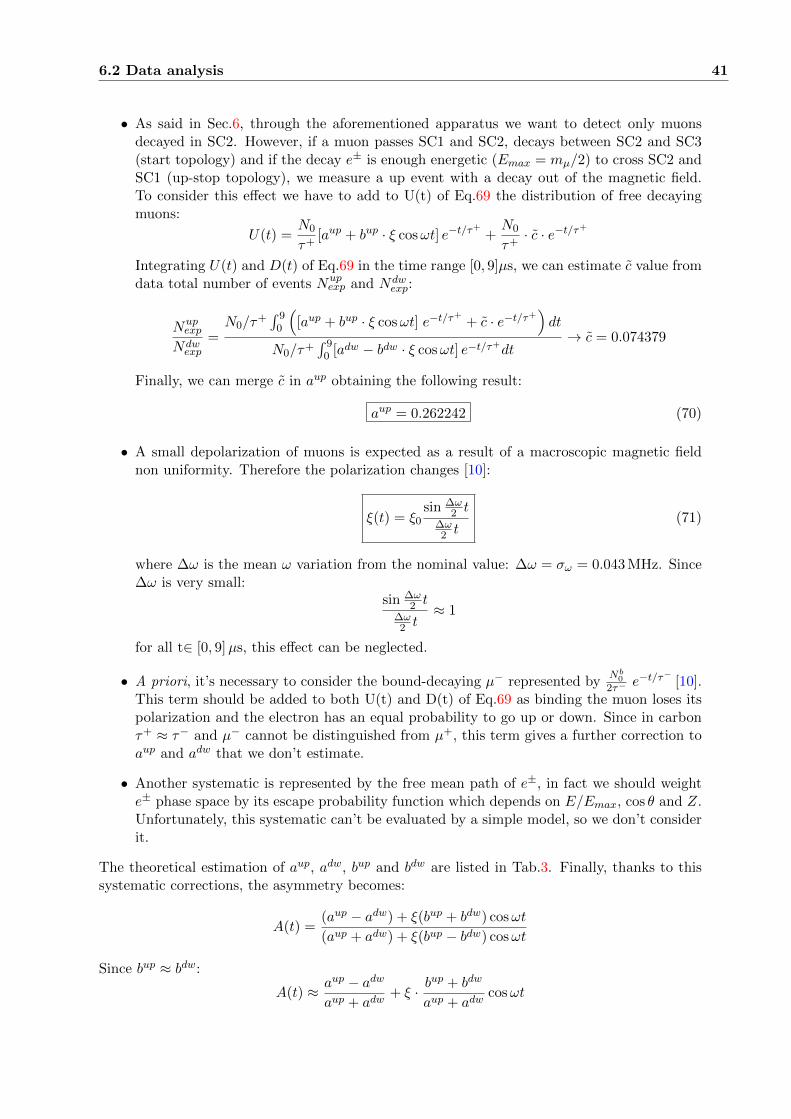
6.2 Data analysis 41
• As said in Sec.6, through the aforementioned apparatus we want to detect only muonsdecayed in SC2. However, if a muon passes SC1 and SC2, decays between SC2 and SC3(start topology) and if the decay e± is enough energetic (Emax = mµ/2) to cross SC2 andSC1 (up-stop topology), we measure a up event with a decay out of the magnetic field.To consider this effect we have to add to U(t) of Eq.69 the distribution of free decayingmuons:
U(t) =N0
τ+[aup + bup · ξ cosωt] e−t/τ
++N0
τ+· c · e−t/τ+
Integrating U(t) and D(t) of Eq.69 in the time range [0, 9]µs, we can estimate c value fromdata total number of events Nup
exp and Ndwexp:
Nupexp
Ndwexp
=N0/τ
+´ 9
0
([aup + bup · ξ cosωt] e−t/τ
++ c · e−t/τ+
)dt
N0/τ+´ 9
0 [adw − bdw · ξ cosωt] e−t/τ+dt→ c = 0.074379
Finally, we can merge c in aup obtaining the following result:
aup = 0.262242 (70)
• A small depolarization of muons is expected as a result of a macroscopic magnetic fieldnon uniformity. Therefore the polarization changes [10]:
ξ(t) = ξ0sin ∆ω
2 t∆ω2 t
(71)
where ∆ω is the mean ω variation from the nominal value: ∆ω = σω = 0.043 MHz. Since∆ω is very small:
sin ∆ω2 t
∆ω2 t
≈ 1
for all t∈ [0, 9]µs, this effect can be neglected.
• A priori, it’s necessary to consider the bound-decaying µ− represented byNb
02τ− e
−t/τ− [10].This term should be added to both U(t) and D(t) of Eq.69 as binding the muon loses itspolarization and the electron has an equal probability to go up or down. Since in carbonτ+ ≈ τ− and µ− cannot be distinguished from µ+, this term gives a further correction toaup and adw that we don’t estimate.
• Another systematic is represented by the free mean path of e±, in fact we should weighte± phase space by its escape probability function which depends on E/Emax, cos θ and Z.Unfortunately, this systematic can’t be evaluated by a simple model, so we don’t considerit.
The theoretical estimation of aup, adw, bup and bdw are listed in Tab.3. Finally, thanks to thissystematic corrections, the asymmetry becomes:
A(t) =(aup − adw) + ξ(bup + bdw) cosωt
(aup + adw) + ξ(bup − bdw) cosωt
Since bup ≈ bdw:
A(t) ≈ aup − adwaup + adw
+ ξ · bup + bdw
aup + adwcosωt
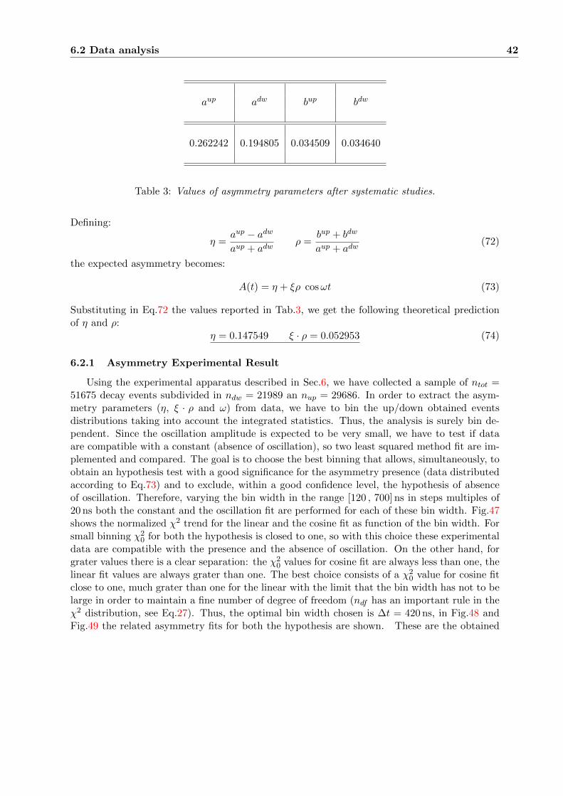
6.2 Data analysis 42
aup adw bup bdw
0.262242 0.194805 0.034509 0.034640
Table 3: Values of asymmetry parameters after systematic studies.
Defining:
η =aup − adwaup + adw
ρ =bup + bdw
aup + adw(72)
the expected asymmetry becomes:
A(t) = η + ξρ cosωt (73)
Substituting in Eq.72 the values reported in Tab.3, we get the following theoretical predictionof η and ρ:
η = 0.147549 ξ · ρ = 0.052953 (74)
6.2.1 Asymmetry Experimental Result
Using the experimental apparatus described in Sec.6, we have collected a sample of ntot =51675 decay events subdivided in ndw = 21989 an nup = 29686. In order to extract the asym-metry parameters (η, ξ · ρ and ω) from data, we have to bin the up/down obtained eventsdistributions taking into account the integrated statistics. Thus, the analysis is surely bin de-pendent. Since the oscillation amplitude is expected to be very small, we have to test if dataare compatible with a constant (absence of oscillation), so two least squared method fit are im-plemented and compared. The goal is to choose the best binning that allows, simultaneously, toobtain an hypothesis test with a good significance for the asymmetry presence (data distributedaccording to Eq.73) and to exclude, within a good confidence level, the hypothesis of absenceof oscillation. Therefore, varying the bin width in the range [120 , 700] ns in steps multiples of20 ns both the constant and the oscillation fit are performed for each of these bin width. Fig.47shows the normalized χ2 trend for the linear and the cosine fit as function of the bin width. Forsmall binning χ2
0 for both the hypothesis is closed to one, so with this choice these experimentaldata are compatible with the presence and the absence of oscillation. On the other hand, forgrater values there is a clear separation: the χ2
0 values for cosine fit are always less than one, thelinear fit values are always grater than one. The best choice consists of a χ2
0 value for cosine fitclose to one, much grater than one for the linear with the limit that the bin width has not to belarge in order to maintain a fine number of degree of freedom (ndf has an important rule in theχ2 distribution, see Eq.27). Thus, the optimal bin width chosen is ∆t = 420 ns, in Fig.48 andFig.49 the related asymmetry fits for both the hypothesis are shown. These are the obtained
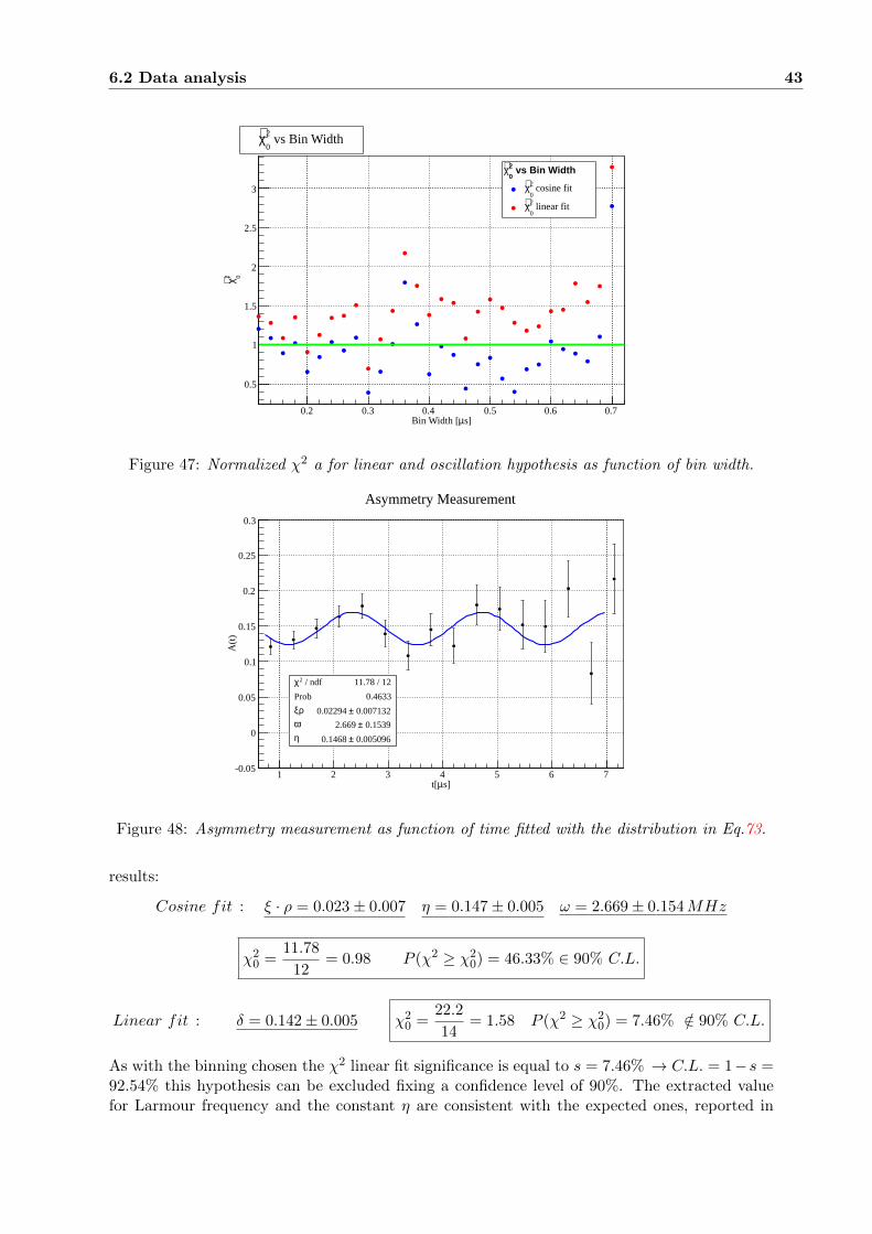
6.2 Data analysis 43
s]µBin Width [0.2 0.3 0.4 0.5 0.6 0.7
2 0χ∼
0.5
1
1.5
2
2.5
3
vs Bin Width2
0χ∼
vs Bin Width2
0χ∼
cosine fit2
0χ∼
linear fit2
0χ∼
Figure 47: Normalized χ2 a for linear and oscillation hypothesis as function of bin width.
s]µt[1 2 3 4 5 6 7
A(t
)
-0.05
0
0.05
0.1
0.15
0.2
0.25
0.3
/ ndf 2χ 11.78 / 12
Prob 0.4633
ρξ 0.007132± 0.02294
ω 0.1539± 2.669
η 0.005096± 0.1468
/ ndf 2χ 11.78 / 12
Prob 0.4633
ρξ 0.007132± 0.02294
ω 0.1539± 2.669
η 0.005096± 0.1468
Asymmetry Measurement
Figure 48: Asymmetry measurement as function of time fitted with the distribution in Eq.73.
results:
Cosine fit : ξ · ρ = 0.023± 0.007 η = 0.147± 0.005 ω = 2.669± 0.154MHz
χ20 =
11.78
12= 0.98 P (χ2 ≥ χ2
0) = 46.33% ∈ 90% C.L.
Linear fit : δ = 0.142± 0.005 χ20 =
22.2
14= 1.58 P (χ2 ≥ χ2
0) = 7.46% /∈ 90% C.L.
As with the binning chosen the χ2 linear fit significance is equal to s = 7.46% → C.L. = 1−s =92.54% this hypothesis can be excluded fixing a confidence level of 90%. The extracted valuefor Larmour frequency and the constant η are consistent with the expected ones, reported in
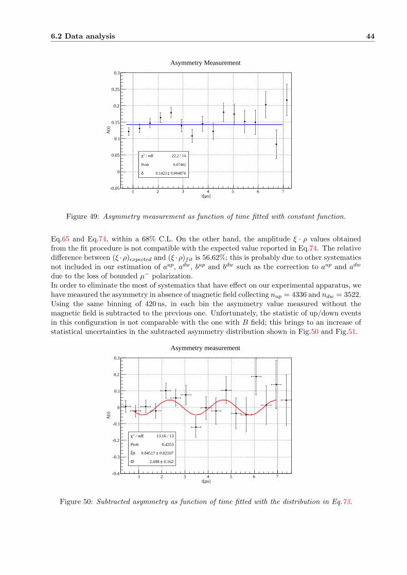
6.2 Data analysis 44
s]µt[1 2 3 4 5 6 7
A(t
)
-0.05
0
0.05
0.1
0.15
0.2
0.25
0.3
/ ndf 2χ 22.2 / 14
Prob 0.07461
δ 0.004874± 0.1423
/ ndf 2χ 22.2 / 14
Prob 0.07461
δ 0.004874± 0.1423
Asymmetry Measurement
Figure 49: Asymmetry measurement as function of time fitted with constant function.
Eq.65 and Eq.74, within a 68% C.L. On the other hand, the amplitude ξ · ρ values obtainedfrom the fit procedure is not compatible with the expected value reported in Eq.74. The relativedifference between (ξ ·ρ)expected and (ξ ·ρ)fit is 56.62%; this is probably due to other systematicsnot included in our estimation of aup, adw, bup and bdw such as the correction to aup and adw
due to the loss of bounded µ− polarization.In order to eliminate the most of systematics that have effect on our experimental apparatus, wehave measured the asymmetry in absence of magnetic field collecting nup = 4336 and ndw = 3522.Using the same binning of 420 ns, in each bin the asymmetry value measured without themagnetic field is subtracted to the previous one. Unfortunately, the statistic of up/down eventsin this configuration is not comparable with the one with B field; this brings to an increase ofstatistical uncertainties in the subtracted asymmetry distribution shown in Fig.50 and Fig.51.
/ ndf 2χ 13.16 / 13
Prob 0.4353
ρξ 0.02107± 0.04517
ω 0.162± 2.698
s]µt[1 2 3 4 5 6 7
A(t
)
-0.4
-0.3
-0.2
-0.1
0
0.1
0.2
0.3
/ ndf 2χ 13.16 / 13
Prob 0.4353
ρξ 0.02107± 0.04517
ω 0.162± 2.698
Asymmetry measurement
Figure 50: Subtracted asymmetry as function of time fitted with the distribution in Eq.73.
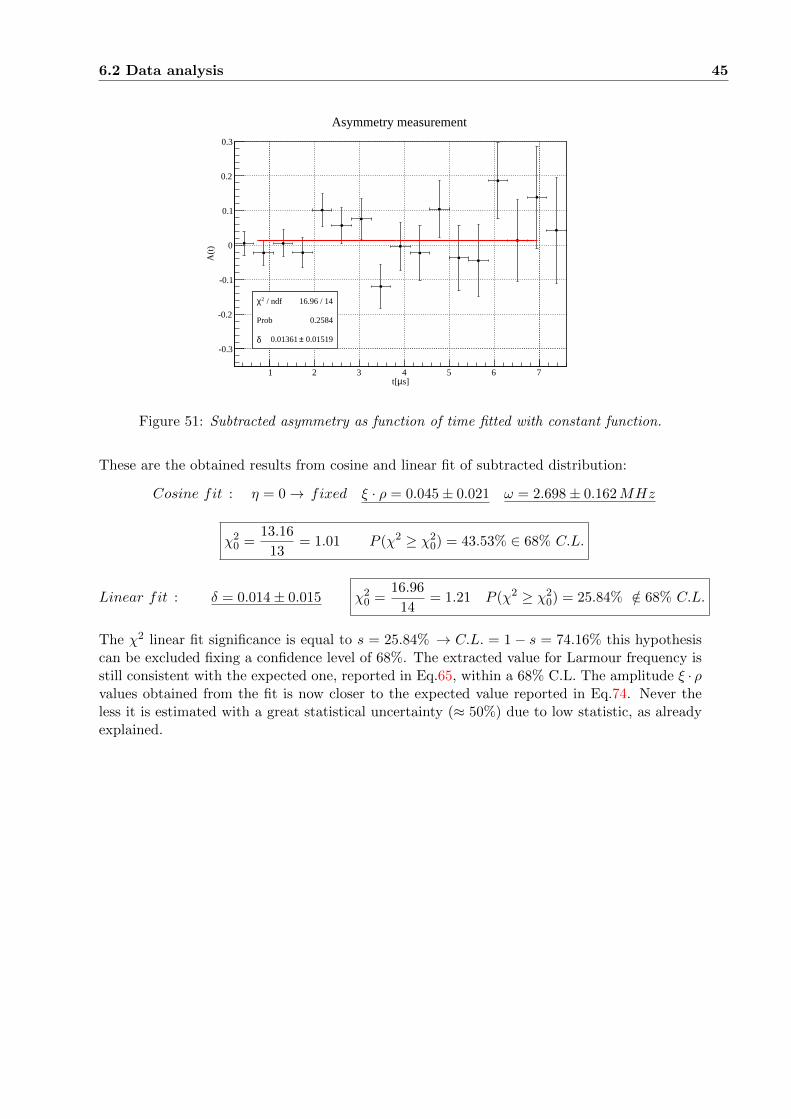
6.2 Data analysis 45
/ ndf 2χ 16.96 / 14
Prob 0.2584
δ 0.01519± 0.01361
s]µt[1 2 3 4 5 6 7
A(t
)
-0.3
-0.2
-0.1
0
0.1
0.2
0.3
/ ndf 2χ 16.96 / 14
Prob 0.2584
δ 0.01519± 0.01361
Asymmetry measurement
Figure 51: Subtracted asymmetry as function of time fitted with constant function.
These are the obtained results from cosine and linear fit of subtracted distribution:
Cosine fit : η = 0→ fixed ξ · ρ = 0.045± 0.021 ω = 2.698± 0.162MHz
χ20 =
13.16
13= 1.01 P (χ2 ≥ χ2
0) = 43.53% ∈ 68% C.L.
Linear fit : δ = 0.014± 0.015 χ20 =
16.96
14= 1.21 P (χ2 ≥ χ2
0) = 25.84% /∈ 68% C.L.
The χ2 linear fit significance is equal to s = 25.84% → C.L. = 1 − s = 74.16% this hypothesiscan be excluded fixing a confidence level of 68%. The extracted value for Larmour frequency isstill consistent with the expected one, reported in Eq.65, within a 68% C.L. The amplitude ξ · ρvalues obtained from the fit is now closer to the expected value reported in Eq.74. Never theless it is estimated with a great statistical uncertainty (≈ 50%) due to low statistic, as alreadyexplained.
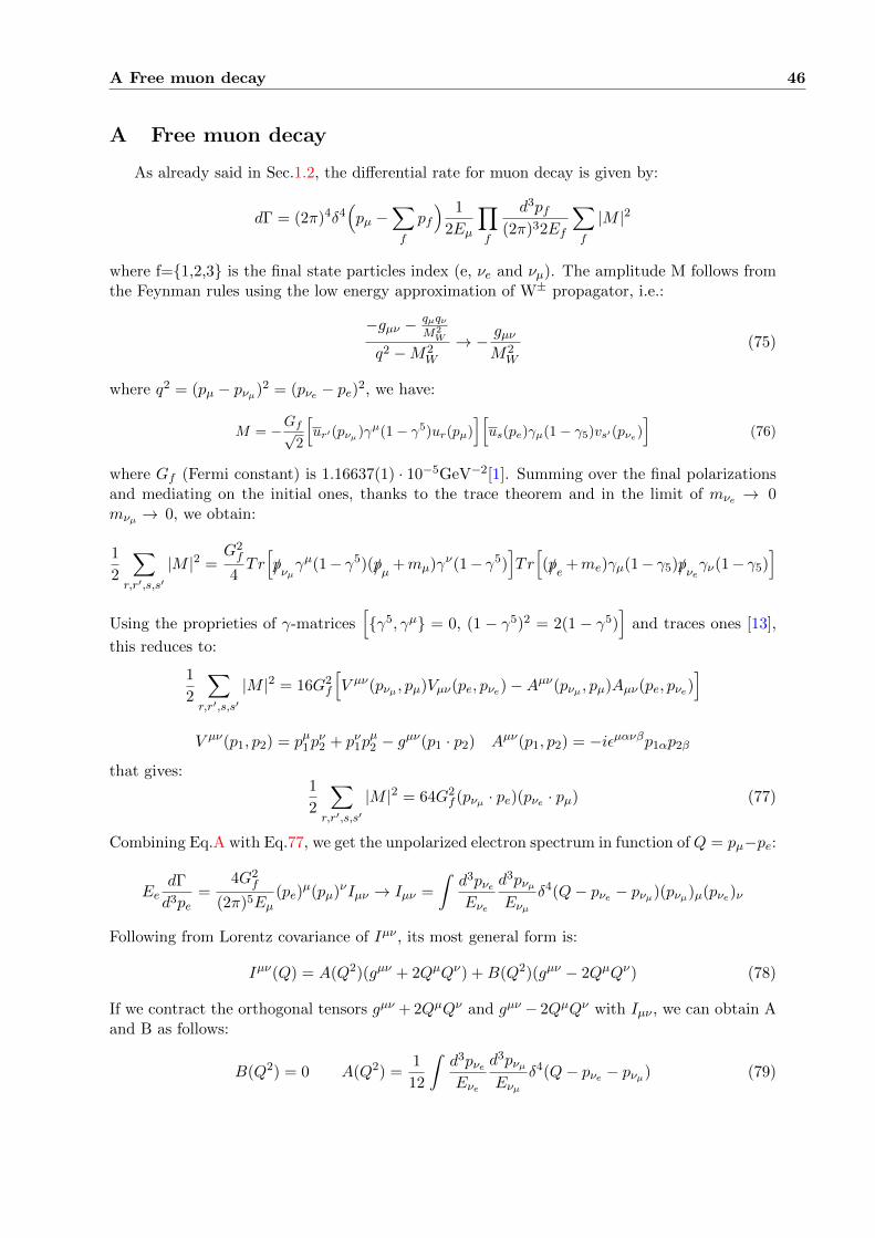
A Free muon decay 46
A Free muon decay
As already said in Sec.1.2, the differential rate for muon decay is given by:
dΓ = (2π)4δ4(pµ −
∑f
pf
) 1
2Eµ
∏f
d3pf(2π)32Ef
∑f
|M |2
where f=1,2,3 is the final state particles index (e, νe and νµ). The amplitude M follows fromthe Feynman rules using the low energy approximation of W± propagator, i.e.:
−gµν − qµqνM2W
q2 −M2W
→ − gµνM2W
(75)
where q2 = (pµ − pνµ)2 = (pνe − pe)2, we have:
M = −Gf√2
[ur′(pνµ)γµ(1− γ5)ur(pµ)
][us(pe)γµ(1− γ5)vs′(pνe)
](76)
where Gf (Fermi constant) is 1.16637(1) · 10−5GeV−2[1]. Summing over the final polarizationsand mediating on the initial ones, thanks to the trace theorem and in the limit of mνe → 0mνµ → 0, we obtain:
1
2
∑r,r′,s,s′
|M |2 =G2f
4Tr[/pνµ
γµ(1− γ5)(/pµ +mµ)γν(1− γ5)]Tr[(/pe +me)γµ(1− γ5)/pνe
γν(1− γ5)]
Using the proprieties of γ-matrices[γ5, γµ = 0, (1 − γ5)2 = 2(1 − γ5)
]and traces ones [13],
this reduces to:
1
2
∑r,r′,s,s′
|M |2 = 16G2f
[V µν(pνµ , pµ)Vµν(pe, pνe)−Aµν(pνµ , pµ)Aµν(pe, pνe)
]V µν(p1, p2) = pµ1p
ν2 + pν1p
µ2 − gµν(p1 · p2) Aµν(p1, p2) = −iεµανβp1αp2β
that gives:1
2
∑r,r′,s,s′
|M |2 = 64G2f (pνµ · pe)(pνe · pµ) (77)
Combining Eq.A with Eq.77, we get the unpolarized electron spectrum in function of Q = pµ−pe:
EedΓ
d3pe=
4G2f
(2π)5Eµ(pe)
µ(pµ)νIµν → Iµν =
ˆd3pνeEνe
d3pνµEνµ
δ4(Q− pνe − pνµ)(pνµ)µ(pνe)ν
Following from Lorentz covariance of Iµν , its most general form is:
Iµν(Q) = A(Q2)(gµν + 2QµQν) +B(Q2)(gµν − 2QµQν) (78)
If we contract the orthogonal tensors gµν + 2QµQν and gµν − 2QµQν with Iµν , we can obtain Aand B as follows:
B(Q2) = 0 A(Q2) =1
12
ˆd3pνeEνe
d3pνµEνµ
δ4(Q− pνe − pνµ) (79)

A Free muon decay 47
Since A(Q2) is Lorentz invariant, we can choose the centre of mass system of the two neutrinos(~pνµ = −~pνe → ~Q = 0), so that:
A(Q2) =1
12
ˆd3pνµEν2µ
δ(Q0 − 2Eνµ) =π
6
ˆ |~pνµ |2E2νµ
dpνµδ(Eνµ −
Q0
2
)=π
6(80)
And the electron spectrum becomes:
EedΓ
d3pe=
4G2f
(2π)5Eµ(pe)
µ(pµ)νIµν → EedΓ
d3pe=
4G2f
(2π)5Eµ
π
6
(Q2(pe · pµ) + 2(Q · pe)(Q · pµ)
)(81)
Finally, we have to integrate Eq.81 over the electron momentum pe in the rest frame of the muonwhere pµ = (mµ,~0), ~pe = − ~pµ and Ee =
mµx2 with x ∈ [0, 1], obtaining:
Γ =2π
3
G2f
(2π)5mµ
ˆpedEedΩ
[(m2
µ +m2e − 2mµEe)mµEe + 2mµ(mµ − Ee)(mµEe −m2
e)]
If we neglect the electron mass term me → 0, pe ≈ Ee =mµx
2 , we arrive to the Fermi formula:
Γ =G2fm
5µ
96π3
ˆ 1
0dxx2(3− 2x) =
G2fm
5µ
192π3=⇒ τ [µ± → e+ νe + νµ] = 2.2µs (82)
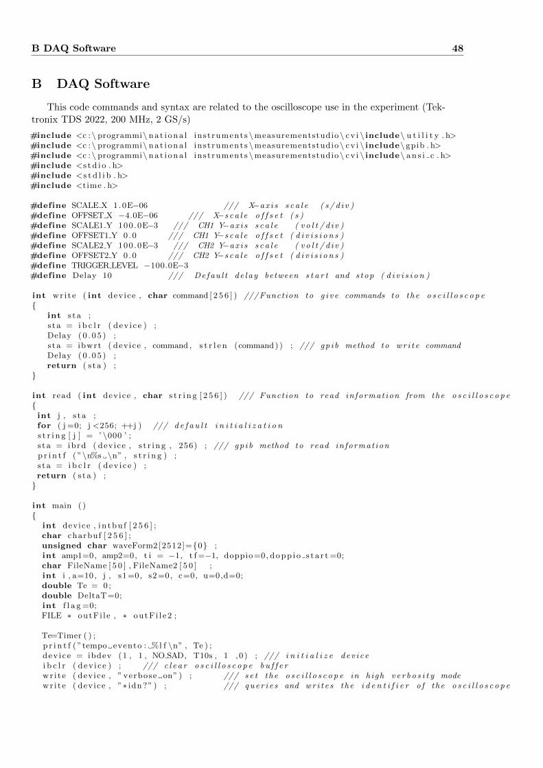
B DAQ Software 48
B DAQ Software
This code commands and syntax are related to the oscilloscope use in the experiment (Tek-tronix TDS 2022, 200 MHz, 2 GS/s)
#include <c :\ programmi\ na t i on a l instruments \measurementstudio\ cv i \ include\ u t i l i t y . h>#include <c :\ programmi\ na t i on a l instruments \measurementstudio\ cv i \ include\ gpib . h>#include <c :\ programmi\ na t i on a l instruments \measurementstudio\ cv i \ include\ a n s i c . h>#include <s t d i o . h>#include <s t d l i b . h>#include <time . h>
#define SCALE X 1.0E−06 /// X−ax i s s c a l e ( s / d i v )#define OFFSET X −4.0E−06 /// X−s c a l e o f f s e t ( s )#define SCALE1 Y 100 .0E−3 /// CH1 Y−ax i s s c a l e ( v o l t / d i v )#define OFFSET1 Y 0 .0 /// CH1 Y−s c a l e o f f s e t ( d i v i s i o n s )#define SCALE2 Y 100 .0E−3 /// CH2 Y−ax i s s c a l e ( v o l t / d i v )#define OFFSET2 Y 0 .0 /// CH2 Y−s c a l e o f f s e t ( d i v i s i o n s )#define TRIGGER LEVEL −100.0E−3#define Delay 10 /// De fau l t de l ay between s t a r t and s top ( d i v i s i o n )
int wr i t e ( int device , char command [ 2 5 6 ] ) ///Function to g i v e commands to the o s c i l l o s c o p e
int s ta ;s ta = i b c l r ( dev i c e ) ;Delay ( 0 . 0 5 ) ;s ta = ibwrt ( device , command , s t r l e n (command) ) ; /// gp i b method to wr i t e commandDelay ( 0 . 0 5 ) ;return ( s ta ) ;
int read ( int device , char s t r i n g [ 2 5 6 ] ) /// Function to read in format ion from the o s c i l l o s c o p eint j , s ta ;for ( j =0; j <256; ++j ) /// d e f a u l t i n i t i a l i z a t i o ns t r i n g [ j ] = ’ \000 ’ ;s ta = ibrd ( device , s t r i ng , 256) ; /// gp i b method to read in format ionp r i n t f ( ”\n%s \n” , s t r i n g ) ;s ta = i b c l r ( dev i c e ) ;return ( s ta ) ;
int main ( )
int device , i n tbu f [ 2 5 6 ] ;char charbuf [ 2 5 6 ] ;unsigned char waveForm2 [2512]=0 ;int amp1=0, amp2=0, t i = −1, t f =−1, doppio =0, d o p p i o s t a r t =0;char FileName [ 5 0 ] , FileName2 [ 5 0 ] ;int i , a=10, j , s1 =0, s2 =0, c=0, u=0,d=0;double Te = 0 ;double DeltaT=0;int f l a g =0;FILE ∗ outFi l e , ∗ outF i l e2 ;
Te=Timer ( ) ;p r i n t f ( ”tempo evento : %l f \n” , Te ) ;dev i c e = ibdev (1 , 1 , NO SAD, T10s , 1 ,0 ) ; /// i n i t i a l i z e dev i c ei b c l r ( dev i c e ) ; /// c l e a r o s c i l l o s c o p e b u f f e rwr i t e ( device , ” verbose on” ) ; /// s e t the o s c i l l o s c o p e in h igh v e r b o s i t y modewr i t e ( device , ”∗ idn ?” ) ; /// que r i e s and wr i t e s the i d e n t i f i e r o f the o s c i l l o s c o p e

B DAQ Software 49
read ( device , charbuf ) ; /// id and in format ionwr i t e ( device , ” f a c t o r y ” ) /// r e s e t s the o s c i l l o s c o p e to d e f a l u t s e t t i n g swr i t e ( device , ” unlock a l l ” ) ;wr i t e ( device , ”ch1 : probe 1” ) ; /// s e t CH1 probe a t t enua t i on to 1wr i t e ( device , ”ch2 : probe 1” ) ; /// s e t CH2 probe a t t enua t i on to 1
for ( i =0; i <256; ++i ) /// Set charbu f to empty vec t o r charbuf [ i ] = ’ \000 ’ ;s p r i n t f ( charbuf , ” h o r i z o n t a l : main : s c a l e %e” , SCALE X ) ; /// Set X−ax i s main s c a l ewr i t e ( device , charbuf ) ;for ( i =0; i <256; ++i ) charbuf [ i ] = ’ \000 ’ ;s p r i n t f ( charbuf , ” h o r i z o n t a l : main : p o s i t i o n %e” , OFFSET X ) ; /// Set X−ax i s o f f s e t andwr i t e ( device , charbuf ) ;for ( i =0; i <256; ++i ) charbuf [ i ] = ’ \000 ’ ;s p r i n t f ( charbuf , ”ch2 : s c a l e %e” , SCALE2 Y ) ; /// s e t CH2 Y−ax i s s c a l ewr i t e ( device , charbuf ) ;for ( i =0; i <256; ++i ) charbuf [ i ] = ’ \000 ’ ;s p r i n t f ( charbuf , ”ch2 : p o s i t i o n %e” , OFFSET2 Y ) ; /// and CH2 Y−ax i s o f f s e twr i t e ( device , charbuf ) ;for ( i =0; i <256; ++i ) charbuf [ i ] = ’ \000 ’ ;s p r i n t f ( charbuf , ”ch1 : s c a l e %e” , SCALE1 Y ) ; /// s e t CH1 Y−ax i s s c a l ewr i t e ( device , charbuf ) ;for ( i =0; i <256; ++i ) charbuf [ i ] = ’ \000 ’ ;s p r i n t f ( charbuf , ”ch1 : p o s i t i o n %e” , OFFSET1 Y ) ; /// s e t CH1 Y−ax i s o f f s e twr i t e ( device , charbuf ) ;
wr i t e ( device , ” t r i g g e r : main : edge : source ext ” ) ; /// Set the t r i g g e r sourcewr i t e ( device , ” t r i g g e r : main : edge : s l ope f a l l ” ) ; /// Set o f t r i g g e r modes on edge s l o p e f a l lfor ( i =0; i <256; ++i ) charbuf [ i ] = ’ \000 ’ ;s p r i n t f ( charbuf , ” t r i g g e r : main : l e v e l %e” , TRIGGER LEVEL) ; /// s e t a d e f a u l t t r i g g e r l e v e lwr i t e ( device , charbuf ) ;
wr i t e ( device , ” data : encdg rpbinary ” ) ; ///Set o f data encoding rpbinary , width 1wr i t e ( device , ” data : width 1” ) ;wr i t e ( device , ” data : s t a r t 1” ) ; /// Set number o f sampled po in t s f o r each waveform (2500)wr i t e ( device , ” data : stop 2500” ) ;wr i t e ( device , ” s e l e c t : ch1 on” ) ; /// Turn on CH1wr i t e ( device , ” s e l e c t : ch2 on” ) ; /// Turn on CH2wr i t e ( device , ” acqu i r e : mode sample” ) ; /// Set a c q u i s i t i o n sample mode wi th s t o p a f t e r sequencewr i t e ( device , ” acqu i r e : s t o p a f t e r sequence ” ) ;s p r i n t f ( FileName , ”C:\\2010−2011\\MuLibero\\Tempo Libero . txt ” ) ; /// Create name o f output f i l es p r i n t f ( FileName2 , ”C:\\2010−2011\\MuLibero\\CH 2 . txt ” ) ;p r i n t f ( ”\n∗ mu −> e ∗\n” ) ;p r i n t f ( ”∗∗∗∗∗∗∗∗∗∗∗∗∗\n” ) ;wr i t e ( device , ” acqu i r e : s t a t e run” ) ; /// Set s t a t e o f the o s c i l l o s c o p e ready to acqu i re
///wi th the s e t t i n g s p r e a v i u s l y chosenp r i n t f ( ” O s c i l l o s c o p e up and ready\n” ) ;Te = Timer ( ) ;p r i n t f ( ”tempo evento : %l f \n” , Te ) ; /// Time taken fo s e t t i n g s
while (1 ) /// i n f i n i t e loop wa i t ing f o r a t r i g g e r event
wr i t e ( device , ” t r i g g e r : s t a t e ?” ) ;ib rd ( device , intbuf , 256) ; /// Read in format ion about the t r i g g e r s t a t ei f ( i n tbu f [4]==172316225)

B DAQ Software 50
++c ; /// Good e x t e r na l t r i g g e r eventp r i n t f ( ” n e : %d\n” , c ) ;Te = Timer ( ) ; /// Abso lu te time o f the eventp r i n t f ( ” t e : %l f \n” , Te ) ;wr i t e ( device , ” data : source ch1” ) ; /// Set CH1 as data sourcewr i t e ( device , ” curve ?” ) ;ib rd ( device , waveForm2 , 2512) ; /// Acquire complete waveform on CH1outF i l e = fopen ( FileName , ”a+” ) ; /// Open the output f i l e keep ing o ld dataoutF i l e2 = fopen ( FileName2 , ”a+” ) ;// f p r i n t f ( ou tF i l e , ”%d ” , c ) ;// f p r i n t f ( ou tFi l e2 , ”%d ” , c ) ;
///START EVENT ANALYSISfor ( s2 =0, i =13; i <2512; ++i ) /// Cycle on waveform po in t s (2500−> r e s o l u t i o n 4ns ) i f ( ( ( ( int ) waveForm2 [ i ] ) < 77) && s2 == 0) /// On Y−ax i s 1 v o l t −> 255 d i v i s i o n . ///So we are l o o k in g f o r a po in t on the waveform under the t r i g g e r t r e s h o l d on CH1.
/// I t depends on which s c i n i t l l a t o r in our measure/// in connected wi th CH1 and i t i s equa l to the t r e s h o l d o f the d i s c r im ina to r
s2=i ;a=i ; /// save time and ampl i tude in format ion o f t h i s po in tamp1 = waveForm2 [ i ] ;for ( j=i +1; j<i +17 && j <2512; ++j ) /// waveform con t r o l goodness . i f (waveForm2 [ j ] < amp1) a
amp1 = waveForm2 [ j ] ;i f (waveForm2 [ j ]>waveForm2 [ i ]&& f l a g ==0) f l a g =1;
t i=s2 ; /// here we con t r o l i f in the next 100 ns the waveform drops under the t r i g g e r l e v e l . /// so we can con t r o l the t a i l Pi le−up
f l a g =0;s2 =0;
/// SEARCHING FOR UP STOP EVENTSfor ( i =2220; i < 2250 ; i++) /// Searching on CH1 near the ” t r i g g e r p o s i t i o n ” a s top s i g n a l i f ( ( ( int ) waveForm2 [ i ] ) < 77 &&s2==0) /// Condit ion f o r a p o s s i b l e s top event s2 =1;amp2 = waveForm2 [ i ] ;for ( j=i +1; j<i +17 && j <2512; ++j ) /// waveform con t r o l goodness . i f (waveForm2 [ j ] < amp2)amp2 = waveForm2 [ j ] ;i f (waveForm2 [ j ]>waveForm2 [ i ] &&f l a g ==0) p r i n t f ( ”up\n” ) ; /// s i g n a l compat i b l e wi th up event
u=1;f l a g =1;t f=i ; /// time o f the s top
wr i t e ( device , ” data : source ch2” ) ; /// Set CH2 as data sourcewr i t e ( device , ” curve ?” ) ;ib rd ( device , waveForm2 , 2512) ; /// Acquire complete waveform on CH2f p r i n t f ( outFi l e2 , ” CH2 \n” ) ;for ( i =13; i <2512; ++i ) /// Save complete waveform on CH2 s2=( int ) waveForm2 [ i ] ;
f p r i n t f ( outFi l e2 , ”%d ” , s2 ) ;
/// SEARCHING FOR DOUBLE START EVENT

B DAQ Software 51
s2 =0;for ( i=a−10; i<a+10; i++) ///Cycle around the the s t a r t p o s i t i o n in a range o f +− 40ns i f ( ( ( int ) waveForm2 [ i ] ) < 115&&s2==0) /// t h r e s h o l d l e v e l f o r a doub le s t a r t event d o p p i o s t a r t =1; /// save in format ion o f doub le s t a r t event
s2 =1;p r i n t f ( ” doppio s t a r t \n” ) ; f l a g =0;s2 =0;
///SEARCHING FOR DOWN STOP EVENT and DOUBLE STOP EVENTfor ( i =2220; i < 2250 ; i++) /// Searching on CH2 near the ” t r i g g e r p o s i t i o n ” a s top s i g n a l i f ( ( ( int ) waveForm2 [ i ] ) < 110 &&s2==0) /// Threshold cond i t i on f o r a p o s s i b l e s top event s2 =1;amp2 = waveForm2 [ i ] ;for ( j=i +1; j<i +17 && j <2512; ++j ) /// waveform con t r o l goodness . i f (waveForm2 [ j ] < amp2)amp2 = waveForm2 [ j ] ;i f (waveForm2 [ j ]>waveForm2 [ i ]&& f l a g ==0) p r i n t f ( ”down\n” ) ; /// s i g n a l compat i b l e wi th down event
f l a g =1;d=1;t f=i ; /// time o f the s topi f (u==1)doppio =1;
p r i n t f ( ” doppio\n ” ) ; /// doub le s top event
i f ( ( u==1&&d==0) | |(u==0&&d==1) | | doppio ==1|| d o p p i o s t a r t==1) /// con t i d i on s sav ing event i f ( t i !=−1&&t f !=−1)DeltaT = ( ( t f−t i+Delay )∗10)/ ( (double ) 2500 ) ; /// Ca l cu l a t i n g time between s t a r t and s top
p r i n t f ( ” t = %l f \n” , DeltaT ) ;f p r i n t f ( outFi l e , ”%l f ” , DeltaT ) ; /// Saving in the output f i l ef p r i n t f ( outFi l e , ”%d ” , u ) ;f p r i n t f ( outFi l e , ”%d ” , d ) ;f p r i n t f ( outFi l e , ”%d ” , d o p p i o s t a r t ) ;f p r i n t f ( outFi l e , ”%d ” , doppio ) ;f p r i n t f ( outFi l e , ”%l f \n” , Te ) ;doppio = 0 ;d o p p i o s t a r t =0;u = 0 ;d=0;t i =−1;t f =−1;Te = 0 ;s2 =0;f l a g =0;f c l o s e ( ou tF i l e ) ; /// Clos ing f i l ef c l o s e ( ou tF i l e2 ) ;wr i t e ( device , ” acqu i r e : s t a t e run” ) ; /// Set s t a t e ready to acqu i r e a f t e r a new t r i g g e rp r i n t f ( ”−−−−−−−−−−−−−−−−\n” ) ;
return ( 0 ) ;
REFERENCES 52
References
[1] K.Nakamura et al.(Particle Data Group). J. Phys. G 37, 075021 (2010).
[2] et al. O. Adriani. Pamela measurements of cosmic-ray proton and helium spectra. Science332, 69 (2011);.
[3] et al. D.J. Bird. The cosmic-ray energy spectrum observed by the fly’s eye. The Astrophys-ical Journal, 424:291-502, 1994 March 20;.
[4] A.O. Weissenberg. “ Muons ”. North Holland Publisher.
[5] R.B. Sutton et al. “measurement of negative muon lifetimes in light isotopes” .
[6] Glenn F. Knoll. “ Radiation Detection and Measurament ”. John Wiley and Sons.
[7] ROOT Reference Guide. http://root.cern.ch/root/htmldoc/TRandom.html.
[8] Minuit2 Package. http://root.cern.ch/root/html518/MINUIT2 Index.html.
[9] W. J. Metzger. “statistical methods in data analysis” . Katholieke Universiteit Ni-jmegen.
[10] R. Turner, C. M. Ankenbrandt, and R. C. Larsen. Polarization of cosmic-ray muons. Phys.Rev. D, 4:17–23, Jul 1971.
[11] L.B. Okun. “ Lepton and Quarks ”. North Holland.
[12] L.D. Landau and E.M. Lifshitz. “ Quantum Mechanics ”. Volume 3, Third Ediction.
[13] F.Mandl and G.Shaw. “ The Quantum Field Theory ”. John Wiley and Sons, AppendixA, Section A.3.