Fire Apparatus Driver/Operator - Pumping Apparatus Task Book

HELSINKI UNIVERSITY OF TECHNOLOGY
Faculty of Electronics, Communications and Automation
Department of Signal Processing and Acoustics
Marko Hiipakka
Measurement Apparatus and ModellingTechniques of Ear Canal Acoustics
Master’s Thesis submitted in partial fulfilment of the requirements for the degree of Master of
Science in Technology.
Espoo, 24 Nov, 2008
Supervisor: Professor Matti Karjalainen
Instructors: D.Sc. (Tech.) Antti Kelloniemi

HELSINKI UNIVERSITY ABSTRACT OF THE
OF TECHNOLOGY MASTER’S THESIS
Author: Marko Tapio Hiipakka
Name of the thesis: Measurement Apparatus and Modelling Techniques of Ear Canal AcousticsDate: 24 Nov, 2008 Number of pages: vii + 85Faculty: Faculty of Electronics, Communication and Automation
Department: Department of Signal Processing and Acoustics
Professorship: S-89
Supervisor: Prof. Matti Karjalainen
Instructors: D.Sc. (Tech.) Antti Kelloniemi
Each one of us perceives the sounds around us differently. The acoustic characteristics of the
outer ear have a significant influence to the sensation of hearing. The tendency of the ear canal
to shape the spectral structure of sounds has not been studied systematically and the role of
the ear canal as a part of the outer ear is not yet completely known. Our research focused on
scrutinizing the effects of varying physical dimensions of the outer ear and particularly those
of the ear canal to the pressure at the eardrum. The main emphasis was on determining the
influence of the length of the ear canal to the frequency response at the eardrum and thereby to
the sensation of hearing. In addition, the eardrum’s damping of the resonance frequencies was
studied.
Two ear canal simulators and one dummy head were manufactured for the pressure frequency
response measurements. The target was to physically model the acoustic behaviour of the
human head, pinna, and ear canal as accurately as possible. In addition, the frequency responses
were measured from the ear canals of human test subjects in various acoustical conditions. A
physics-based computational model and equations of the physics of sound were used to validate
the results obtained from the measurements.
The behaviour of the ear canal was investigated in normal listening conditions as well as in free
field conditions. In addition, the behaviour was studied in a situation where the canal entrance
was blocked with an insert earphone. A special pair of earphones with in-ear microphones
was constructed for this purpose. The earphone was also used for studying two important
phenomena related to insert earphones, namely the occlusion effect and sound leakage.
From our research we may conclude that the physical dimensions and especially the length of
the ear canal have a considerable effect to the pressure frequency response at the eardrum. In
addition, we may conclude, that it is possible to accurately model the acoustic behaviour of the
human outer ear with physical simulators.
Keywords: Ear canal, Outer ear, Eardrum, Frequency response.
i

TEKNILLINEN KORKEAKOULU DIPLOMITYÖN TIIVISTELMÄ
Tekijä: Marko Tapio Hiipakka
Työn nimi: Korvakäytävän akustisten ominaisuuksien mittaus ja mallinnus
Päivämäärä: 24.11.2008 Sivuja: vii + 85Tiedekunta: Elektroniikan, tietoliikenteen ja automaation tiedekunta
Laitos: Signaalinkäsittelyn ja akustiikan laitos
Professuuri: S-89
Työn valvoja: Prof. Matti Karjalainen
Työn ohjaajat: TkT Antti Kelloniemi
Ulkokorvan akustiset ominaisuudet vaikuttavat merkittävästi ihmisen kuuloaistimukseen. Yk-
silölliset erot ulkokorvan rakenteissa ovat yksi syy siihen, että kuulemme meitä ympäröivät ää-
net hieman eri lailla. Korvakäytävän taipumusta muokata kuulemiemme äänten spektriraken-
netta on tutkittu vähän, eikä sen akustisia ominaisuuksia tunneta vielä täysin. Tutkimuksessam-
me keskityttiin kartoittamaan ulkokorvan ja erityisesti korvakäytävän fyysisten ulottuvuuksien
vaikutusta tärykalvolla mitattavaan äänipaineeseen. Tutkimuksen pääpainona oli selvittää kor-
vakäytävän pituuden vaikutus taajuusvasteeseen tärykalvolla ja sitä kautta kuuloaistimukseen.
Lisäksi tutkittiin tärykalvon aiheuttamaa vaimennusta korvakäytävän resonansseihin.
Taajuusvasteiden mittauksia varten rakennettiin kaksi uudentyyppistä korvakäytäväsimulaatto-
ria sekä yksi keinopää. Tavoitteena oli mallintaa fyysisesti ihmisen pään, korvalehden ja korva-
käytävän akustinen käyttäytyminen mahdollisimman tarkasti. Lisäksi tutkimuksessa käytettiin
koehenkilöitä, joiden korvakäytävien taajuusvasteita mitattiin erilaisissa olosuhteissa. Korva-
käytäväsimulaattorin laskennallinen malli sekä äänen fysiikan laskukaavat toimivat mittaustu-
losten teoreettisina perusteluina.
Korvakäytävän käyttäytymistä tutkittiin normaaleissa kuunteluolosuhteissa ja vapaakenttäolo-
suhteissa. Lisäksi tutkittiin tilannetta, jossa korvakäytävään on asetettu korvakäytäväkuuloke
(engl. “insert earphone”). Tätä käyttötilannetta ja sen tutkimista varten valmistettiin korva-
käytävämikrofonit sisältävä korvakäytäväkuulokepari, jolla tutkittiin myös kuulokekuuntelun
kannalta tärkeitä okkluusioilmiötä ja äänen vuotoa.
Tutkimuksen lopputuloksena voidaan todeta, että ulkokorvan ulottuvuuksilla ja erityisesti kor-
vakäytävän pituudella on suuri merkitys taajuusvasteeseen tärykalvolla. Lisäksi voidaan todeta,
että fyysisillä simulaattoreilla on mahdollista tarkasti mallintaa ihmisen ulkokorvan akustinen
käyttäytyminen.
Avainsanat: Korvakäytävä, Ulkokorva, Tärykalvo, Taajuusvaste.
ii

Acknowledgements
Research for this Master’s thesis was conducted in the Department of Signal Processing and
Acoustics at the Helsinki University of Technology with funding from Nokia Oyj.
I want to thank Professor Matti Karjalainen for his enthusiastic participation in the planning,
research and practical realizations needed for this Thesis to be completed. In addition, his indis-
pensable guidance and supervision have helped in solving theoretical and practical problems.
I wish to thank Dr. Antti Kelloniemi for sharing his expertise and for instructions as to research
directions. My gratitude also goes to Dr. Jouni Knuuttila, Jarkko Kuntanen, Heidi Linden and
Timo Toivanen for a successful cooperation.
I would also like to thank my co-workers Miikka Tikander, Jussi Rämö and Ville Riikonen for
cooperation and shared efforts within our research. I also have the staff and co-researchers of
the Department of Signal Processing and Acoustics to thank for help and support, and also for
the great spirit you have built up at the ‘laboratory’.
I am deeply indebted to friends, family and relatives who have supported me on my path to
graduation.
Finally, I would like to thank the Polytech Choir as well as Driving School’s principal Veikko
Sompa and his pupils for their irrecoverable help in the avoidance of an overhasty graduation.
Otaniemi, 24 November, 2008
Marko “Magge” Tapio Hiipakka
iii

Contents
Abbreviations vii
1 Introduction 1
2 Acoustics of hearing 3
2.1 Sound and hearing . . . . . . . . . . . . . . . . . . . . . . . . . . . . . . . . 3
2.2 Outer ear . . . . . . . . . . . . . . . . . . . . . . . . . . . . . . . . . . . . . 5
2.2.1 Pinna . . . . . . . . . . . . . . . . . . . . . . . . . . . . . . . . . . . 5
2.2.2 Ear canal . . . . . . . . . . . . . . . . . . . . . . . . . . . . . . . . . 5
2.2.3 Eardrum . . . . . . . . . . . . . . . . . . . . . . . . . . . . . . . . . . 7
2.3 Middle ear . . . . . . . . . . . . . . . . . . . . . . . . . . . . . . . . . . . . . 8
2.4 Inner ear . . . . . . . . . . . . . . . . . . . . . . . . . . . . . . . . . . . . . . 9
2.4.1 Inner ear structure . . . . . . . . . . . . . . . . . . . . . . . . . . . . 9
2.4.2 Inner ear function . . . . . . . . . . . . . . . . . . . . . . . . . . . . . 11
2.5 Sound source localization . . . . . . . . . . . . . . . . . . . . . . . . . . . . . 11
2.5.1 Binaural cues . . . . . . . . . . . . . . . . . . . . . . . . . . . . . . . 12
2.5.2 Monaural cues, HRTF’s . . . . . . . . . . . . . . . . . . . . . . . . . 13
2.5.3 The precedence effect . . . . . . . . . . . . . . . . . . . . . . . . . . 14
3 Headphone and microphone technology 16
3.1 Headphones . . . . . . . . . . . . . . . . . . . . . . . . . . . . . . . . . . . . 16
3.1.1 Headphone categories . . . . . . . . . . . . . . . . . . . . . . . . . . 16
3.1.2 Headphone transducers . . . . . . . . . . . . . . . . . . . . . . . . . . 17
3.1.3 Pressure Chamber Effect . . . . . . . . . . . . . . . . . . . . . . . . . 19
3.2 Microphones . . . . . . . . . . . . . . . . . . . . . . . . . . . . . . . . . . . 20
iv

3.2.1 Microphone categories . . . . . . . . . . . . . . . . . . . . . . . . . . 20
3.2.2 Microphone sensitivity . . . . . . . . . . . . . . . . . . . . . . . . . . 22
3.2.3 Microphone directional sensitivity . . . . . . . . . . . . . . . . . . . . 23
4 Outer ear models 24
4.1 Physical simulators . . . . . . . . . . . . . . . . . . . . . . . . . . . . . . . . 24
4.1.1 Dummy heads . . . . . . . . . . . . . . . . . . . . . . . . . . . . . . 24
4.1.2 Ear canal simulators . . . . . . . . . . . . . . . . . . . . . . . . . . . 26
4.1.3 Tubes as ear canal simulators . . . . . . . . . . . . . . . . . . . . . . . 27
4.1.4 Adjustable ear canal simulator (Adecs) . . . . . . . . . . . . . . . . . 27
4.1.5 Multi-adjustable ear canal simulator (Madecs) . . . . . . . . . . . . . . 28
4.1.6 Artificial pinnas . . . . . . . . . . . . . . . . . . . . . . . . . . . . . . 30
4.1.7 Dummy head with adjustable ear canal (Dadec) . . . . . . . . . . . . . 30
4.2 Computational modelling . . . . . . . . . . . . . . . . . . . . . . . . . . . . . 31
4.2.1 Lumped element and transmission line modelling . . . . . . . . . . . . 31
4.2.2 Estimation of pressure at eardrum . . . . . . . . . . . . . . . . . . . . 36
5 Measurements 38
5.1 Measurement equipment and technology . . . . . . . . . . . . . . . . . . . . . 38
5.1.1 Equipment and software . . . . . . . . . . . . . . . . . . . . . . . . . 38
5.1.2 Earphone with fitted in-ear microphone (Efim) . . . . . . . . . . . . . 39
5.1.3 Measurement environments . . . . . . . . . . . . . . . . . . . . . . . 41
5.2 Acoustic properties of open ear canal . . . . . . . . . . . . . . . . . . . . . . . 41
5.2.1 Frequency response at the ear canal entrance . . . . . . . . . . . . . . 41
5.2.2 Frequency responses along the canal . . . . . . . . . . . . . . . . . . . 46
5.2.3 Frequency response at the eardrum . . . . . . . . . . . . . . . . . . . . 49
5.2.4 Effect of different outer ear shapes . . . . . . . . . . . . . . . . . . . . 53
5.2.5 Effect of drum impedance . . . . . . . . . . . . . . . . . . . . . . . . 57
5.2.6 A computational model . . . . . . . . . . . . . . . . . . . . . . . . . . 59
5.3 Acoustic properties of blocked ear canal . . . . . . . . . . . . . . . . . . . . . 60
5.3.1 Frequency responses of blocked ear canal simulators . . . . . . . . . . 63
5.3.2 Frequency responses of human ears . . . . . . . . . . . . . . . . . . . 65
5.3.3 Effect of eardrum impedance . . . . . . . . . . . . . . . . . . . . . . . 67
v

5.3.4 Effect of canal shape . . . . . . . . . . . . . . . . . . . . . . . . . . . 70
5.3.5 Leakage . . . . . . . . . . . . . . . . . . . . . . . . . . . . . . . . . . 71
5.3.6 Occlusion effect . . . . . . . . . . . . . . . . . . . . . . . . . . . . . 71
6 Conclusions and Future Work 73
6.1 Summary . . . . . . . . . . . . . . . . . . . . . . . . . . . . . . . . . . . . . 73
6.2 Conclusions . . . . . . . . . . . . . . . . . . . . . . . . . . . . . . . . . . . . 74
6.3 Future Work . . . . . . . . . . . . . . . . . . . . . . . . . . . . . . . . . . . . 75
A Test subjects 80
B Figures 81
vi

Abbreviations
Adecs Adjustable ear canal simulator
B&K Brüel & Kjær
Dadec Dummy head with adjustable ear canals
Efim Earphone with fitted in-ear microphone
FFT Fast Fourier Transform
HATS Head and Torso Simulator
HRTF Head-related transfer function
IEC International Electrotechnical Commission
ILD Interaural level difference
ITD Interaural time difference
ITU International Telecommunication Union
Madecs Multi-adjustable ear canal simulator
SPL Sound pressure level
vii
Chapter 1
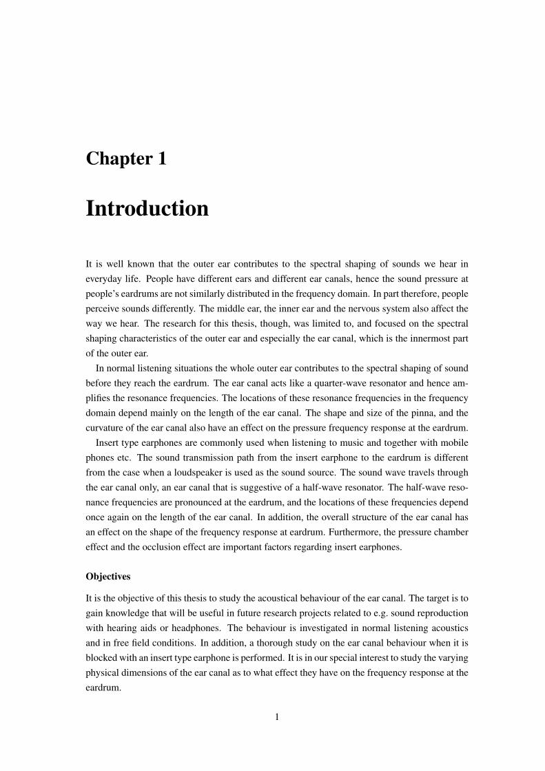
Introduction
It is well known that the outer ear contributes to the spectral shaping of sounds we hear in
everyday life. People have different ears and different ear canals, hence the sound pressure at
people’s eardrums are not similarly distributed in the frequency domain. In part therefore, people
perceive sounds differently. The middle ear, the inner ear and the nervous system also affect the
way we hear. The research for this thesis, though, was limited to, and focused on the spectral
shaping characteristics of the outer ear and especially the ear canal, which is the innermost part
of the outer ear.
In normal listening situations the whole outer ear contributes to the spectral shaping of sound
before they reach the eardrum. The ear canal acts like a quarter-wave resonator and hence am-
plifies the resonance frequencies. The locations of these resonance frequencies in the frequency
domain depend mainly on the length of the ear canal. The shape and size of the pinna, and the
curvature of the ear canal also have an effect on the pressure frequency response at the eardrum.
Insert type earphones are commonly used when listening to music and together with mobile
phones etc. The sound transmission path from the insert earphone to the eardrum is different
from the case when a loudspeaker is used as the sound source. The sound wave travels through
the ear canal only, an ear canal that is suggestive of a half-wave resonator. The half-wave reso-
nance frequencies are pronounced at the eardrum, and the locations of these frequencies depend
once again on the length of the ear canal. In addition, the overall structure of the ear canal has
an effect on the shape of the frequency response at eardrum. Furthermore, the pressure chamber
effect and the occlusion effect are important factors regarding insert earphones.
Objectives
It is the objective of this thesis to study the acoustical behaviour of the ear canal. The target is to
gain knowledge that will be useful in future research projects related to e.g. sound reproduction
with hearing aids or headphones. The behaviour is investigated in normal listening acoustics
and in free field conditions. In addition, a thorough study on the ear canal behaviour when it is
blocked with an insert type earphone is performed. It is in our special interest to study the varying
physical dimensions of the ear canal as to what effect they have on the frequency response at the
eardrum.
1

CHAPTER 1. INTRODUCTION 2
Furthermore, the goal of the research related to this thesis is to model the ear canal and the
whole outer ear as accurately as possible. Two approaches are applied: the building of physical
simulators and physics-based computational modelling, the emphasis being on simulators. The
aim is to validate the use of both approaches as parallel modelling techniques.
Finally, we hope that the results obtained in our research can help focusing future research
projects.
Outline
This thesis consists of three main parts; first, the basics of hearing and technologies related to
this thesis are presented. In the second part, a look at physical simulation and physics-based
computational modelling is taken. In the third part, the acoustic behaviour of the outer ear and
the ear canal is viewed through measurement results.
The basics of sound and hearing are overviewed in Chapter 2. The different parts of the human
auditory system from the pinna to the inner ear are presented. In addition, the basics of binaural
hearing are briefly presented. Headphone and microphone technologies are presented in Chapter
3.
Ear canal simulators, dummy heads and physics-based computational modelling are presented
in Chapter 4. The physical simulators used in the research for this thesis were self-made and they
were intended to copy the acoustical behaviour of the outer ear.
In Chapter 5 the acoustic behaviour of the ear canal in normal listening conditions and when
the canal entrance is blocked with an insert earphone is studied. The novel ear canal simulators
and a dummy head were used for measuring the effects of varying physical parameters such as
the ear canal length and the overall shape of the outer ear.
Conclusions and future work scenarios are discussed in Chapter 6.

Chapter 2
Acoustics of hearing
The basics in the acoustics of hearing and the human auditory system are reviewed in this Chap-
ter. First, the basics of sound and hearing are presented. The characteristics of the different parts
of the human ear, as depicted in Figure 2.1, are described briefly.
Figure 2.1: The ear consists of external, middle and inner structures. [3]
The effects of the pinna, the head and the shoulders are reviewed because of their overall effect
on the transfer function from a sound source to the ear canal but also due to their significance
especially in directional hearing. A brief look at this field of acoustics is taken, even though it is
not within our main area of focus.
2.1 Sound and hearing
Sound can refer to either an auditory sensation in the brain or the disturbance in a medium that
causes this sensation [55]. Hearing is the process by which the ear transforms sound vibrations
into nerve impulses that are delivered to the brain and interpreted as sounds. Sound waves are
produced when vibrating objects produce pressure pulses of vibrating air. The auditory system
can distinguish different subjective aspects of a sound, such as its loudness and pitch. [16]
3

CHAPTER 2. ACOUSTICS OF HEARING 4
Pitch is the subjective perception of the frequency, which in turn is measured in cycles per
second, or Hertz (Hz). The normal human audible range extends from about 20 to 20,000 Hz, but
the human ear is most sensitive to frequencies of 1,000 to 4,000 Hz. Loudness is the perception
of the intensity of sound, related to the pressure produced by sound waves on the tympanic
membrane. The pressure level of sound is measured in decibels (dB), a unit for comparing the
intensity of a given sound with a sound that is just perceptible to the normal human ear at a
frequency in the range to which the ear is most sensitive. On the decibel scale, the range of
human hearing extends from 0 dB, which represents the auditory threshold, to about 130 dB, the
level at which sound becomes painful. [16] [55]
In order for a sound to be transmitted to the central nervous system, the energy of the sound
undergoes three transformations. First, the air vibrations are converted to vibrations of the tym-
panic membrane and ossicles of the middle ear. These, in turn, become vibrations in the fluid
within the cochlea. Finally, the fluid vibrations set up travelling waves along the basilar mem-
brane that stimulate the hair cells of the organ of Corti. These cells convert the sound vibrations
to nerve impulses in the fibres of the cochlear nerve, which transmits them to the brain stem,
from which they are relayed, after extensive processing, to the primary auditory area of the cere-
bral cortex, the ultimate centre of the brain for hearing. Only when the nerve impulses reach this
area does the listener become aware of the sound. A simplified scheme of the human peripheral
hearing is depicted in Figure 2.2. [30] [16]
Figure 2.2: Structure of the human peripheral hearing. [30]
The ear has an enormous range of response, both in frequency and in intensity. The frequency
range of human hearing extends over three orders of magnitude, from about 20 Hertz to about 20
kHz. The minimum audible pressure amplitude, at the threshold of hearing, is about 10−5 Pascal,or about 10−10 standard atmosphere, corresponding to a minimum intensity of about 10−12Wattper square metre. The pressure fluctuation associated with the threshold of pain, meanwhile, is
over 10 Pascals, which is one million times the pressure or one trillion times the intensity of
the threshold of hearing. In both cases, the enormous dynamic range of the ear dictates that its
response to changes in frequency and intensity must be nonlinear. [16]
Relating frequency to pitch as perceived by the musician, two notes will sound similar if they
are spaced apart in frequency by a factor of two, or octave. This means that the tuning of musical
scales and musical intervals is associated with frequency ratios rather than absolute frequency
differences. [16]

CHAPTER 2. ACOUSTICS OF HEARING 5
The audio frequency range comprises nearly nine octaves. Over most of this range, the min-
imum change in the frequency of a sinusoidal tone that can be detected by the ear, called the
just noticeable frequency difference, is about 0.5 percent of the frequency of the tone, or about
one-tenth of a musical half-step. [16]
2.2 Outer ear
In spoken language, the word “ear” is used referring only to the visible part of the ear. In
science, the visible part is named the pinna, which is Latin for “feather” [37]. From an acoustic
perspective, an important part of the pinna is the concha, which is the horn-like cavity that
connects the pinna and the ear canal. Even thought the ear canal is not visible to the plain eye it
is still a part of the outer ear. The outer ear ends at the eardrum.
2.2.1 Pinna
The pinna, which is also known as “auricle”, acts as a sound reflector and it is formed primarily
of cartilage without any useful muscles. The pinna works differently for low and high frequen-
cies. Sound waves with frequencies below 1 kHz are not affected by the pinna. Above 1 kHz
and especially around the important speech frequencies (2 kHz to 3 kHz) the sound pressure is
boosted significantly. Here the behaviour is similar to a reflecting dish as it directs sounds toward
the ear canal. [17]
The direct and the reflected signals arrive to the ear canal mainly in phase. However, at
high frequencies, the reflected waves enter the ear canal at a very slight delay, which translates
into phase cancellation or destructive interference. The greatest interference occurs when the
difference in total path length is a half wavelength. This produces a “pinna notch” around 7-
10 kHz. The boosting effect starts at frequencies above 1 kHz, since the size of the pinna is
noticeable only when wavelength is close to or less than four times the size of the pinna. The
wavelength of a sound wave is
λ =v
f, (2.1)
where v is the speed of sound, and f is the frequency of the sound signal. In 20◦C air at sea level,the speed of sound is approximately 343 m/s. The pinna offers a certain differentiation of sounds
from the front as compared to sound from the rear. The rather significant impact of individual
pinnas to directional hearing is discussed in Chapter 2.5.
The size and shape of the pinna varies between individuals. Furthermore, the pinna tends to
grow bigger when people age. The concha (or the bowl), which is the part of the pinna that is
closest to the ear canal, forms a horn-like entrance to the ear canal.
2.2.2 Ear canal
The ear canal (external auditory meatus, external acoustic meatus) can be described or modelled
as a tube that extends from the concha to the eardrum. The ear canal acts as a quarter-wave

CHAPTER 2. ACOUSTICS OF HEARING 6
resonator and it boosts the incoming sound around frequencies the wavelength, λ, of which are
close to
λ = 4 · n · L, (2.2)
where L is the length of the ear canal and n is an odd number (1, 3, 5...).An average human ear canal is 26 mm in length and 7 mm in diameter. The outer part of the
canal consists of a cartilaginous soft body and a 0.5 - 1.0 mm thick skin with glands and hair
follicles. The glands produce ear wax, which has an important role in keeping the ear canal clean
and protecting it from bacteria, fungi and insects. The outer soft part of the canal forms one third
to one half of total canal length. The remaining inner part of the canal rests on the opening of
the bony skull and the skin in this part of the canal is tightly applied to the bone. The skin here
is approximately 0.2 mm thick and it is easily injured or ruptured. [4]
Figure 2.3: Pinna and ear canal seen from the front. [60]
In literature, the ear canal is often depicted with various different interpretations, which is
because ear canals are different in size and shape between individuals. A slightly curved tube,
as in Figure 2.3 is to be the most common shape of the canal when viewed from the front.
Figure 2.4: Medial section of the outer ear and ear canal seen from the top of the head. [44]
Seen from below, there are two more or less pronounced bends (see Figure 2.4), the first of
which is in the lateral part of the canal near the canal entrance. The second bend is placed near
the junction of the cartilage and the bony parts. Usually the ear canal narrows down towards the
second bend. This notwithstanding a flaring sometimes occurs from the first bend towards the
second bend, which can be seen from e.g. deep impressions of the canal. Furthermore, the shape
of the ear canal might change when moving the jaws. [4] [44]
The eardrum terminates the ear canal (as depicted in Figure 2.3) and hence separates it from
the middle ear cavity.

CHAPTER 2. ACOUSTICS OF HEARING 7
2.2.3 Eardrum
The eardrum (tympanic membrane, tympanum, myrinx), is a thin membrane that separates the
external ear from the middle ear. It transmits sound from the ear canal to the ossicles inside the
middle ear. The malleus bone bridges the gap between the eardrum and the other ossicles.
The eardrum is a smooth, translucent membrane with an average thickness of 0.074 mm. The
shape is elliptical the height being approximately 10 mm and the width 8 mm. The mass of the
eardrum is approximately 14 mg.
Figure 2.5: A photo of a human eardrum. The different parts are annotated as follows: An -Annulus fibrosus; Lpi - Long process of incus, which is sometimes visible through a healthytranslucent drum; Um - Umbo, the end of the malleus handle and the centre of the drum; Lr- Light reflex, also known as Antero-inferioirly or Cone of light; Lp - Lateral process of themalleus; At - Attic also known as Pars flaccida; Hm - handle of the malleus, also known asmanubrium of malleus. [61]
One rather important characteristic is that the eardrum does not terminate the canal perpen-
dicularly. It may be even be considered to form the innermost part of the canal wall, a canal that
converges or narrows towards the lower end of the canal. In other words, the eardrum is slanted
so that the upper wall of the ear canal is shorter than the lower part of the wall. The slanting
forms an angle of approximately 40 ◦ with the lower part of the ear canal wall. This angle issmaller at birth, however, when the eardrum is nearly horizontal.
The eardrum is concave, which means that it is inwardly displaced by about 2 mm. At its
centre, there is an outshot caused by the inferior tip of the handle of the malleus.
Considering its thinness, the eardrum is tough and resilient. This is due to the layered archi-
tecture consisting of an outer cutaneous layer, a middle fibrous layer (or lamina propria) and an
internal layer (or serous membrane). The cutaneous (skin-related) layer is continuous with the
lining of the external auditory canal and the internal layer is continuous with the lining of the
middle ear. Rupture or perforation of the eardrum can lead to conductive hearing loss.

CHAPTER 2. ACOUSTICS OF HEARING 8
The eardrum can be divided into four quadrants, with the centre of the four quadrants being
the umbo. The chorda tympani nerve, and arteries pass through the layers of the superior portion
of the membrane. Therefore, when the tympanic membrane needs to be operated on, cuts will
always be made through the inferior and posterior part of the membrane to avoid the vasculature,
nerves, and bones associated with the membrane. [4]
Figure 2.6: An artificial eardrum produced using human skin cells. [2]
The researchers in Ear Science Institute of Australia have introduced a process, which has
allowed them to produce a new eardrum using human skin cells. A specimen is depicted in
Figure 2.6. An artificial eardrum could be used for replacing a damaged eardrum. [2]
Acoustic reflex
At high sound pressure levels the muscles of the middle ear, the tensor tympani and the stapedius,
can influence the transmission of sound by the ossicular chain. Contraction of the tensor tympani
pulls the handle of the malleus inward and tenses the eardrum. Contraction of the stapedius pulls
the stapes footplate outward from the oval window and thereby reduces the intensity of sound
reaching the cochlea. The stapedius responds reflexly with quick contraction to sounds of high
intensity applied either to the same ear or to the opposite ear. For sinusoidal stimulus, this effect
starts between 90 and 95 dB SPL. The reflex has been likened to the blink of the eye or the
constriction of the pupil of the eye in response to light and is thought to have protective value.
[16]
2.3 Middle ear
The middle ear is limited by the eardrum and the oval window of the cochlea. The air-filled
space of the middle ear is also known as the tympanic cavity, or cavum tympani.
The middle ear contains three ossicles - the small bones found in the ears of all mammals (the
root word ‘os’ refers to bones). These bones are the smallest bones in a person’s body and they
couple vibration of the eardrum into waves in the fluid and membranes of the inner ear. The
malleus (hammer) is the bone attached to the eardrum and the second ossicle, the incus (anvil)
as depicted in Figure 2.7. The third of the ossicles is the stapes (stirrup), which is connected to
the inner ear. The ossicles together are a very important part of the hearing system. They act as
a lever that boosts the very small pressure exerted by a sound wave on the eardrum into as much
as 30 times bigger a pressure at the oval window of the inner ear. This magnification is mainly

CHAPTER 2. ACOUSTICS OF HEARING 9
due to the difference in the areas of the eardrum and the oval window, the lever action of the
ossicles provides a force multiplication factor of about 1.5. [55]
Figure 2.7: The eardrum transfers the sound vibration to the ossicles. From left to right: eardrum,
malleus, incus and stapes. [48]
When the eardrum vibrates, it pushes the malleus, which then begins to vibrate in sync with
the sound. When the malleus vibrates against the incus, it also begins to vibrate and transfers the
vibration to the last ossicle, the stapes. The plate at the end of the stapes lies on top of the oval
window of the cochlea and the vibration of the plate creates pressure waves into the fluid-filled
cavity of the cochlea.
The Eustachian tube (auditory tube, pharyngotympanic tube) is a tube that joins the tympanic
cavity with the nasal cavity (nasopharynx). Usually the Eustachian tube is closed, but it can
open to keep the pressure difference between the two cavities at minimum. In addition, mucus (a
slimy substance, typically not miscible with water, secreted by mucous membranes and glands
for lubrication, protection, etc.) is transferred through the Eustachian tube from the middle ear.
The Eustachian tube of an adult is approximately 35 mm long. The upper one third of the tube
is made of bone and the rest is composed of cartilage.
2.4 Inner ear
2.4.1 Inner ear structure
The cochlea is a small threaded conical chamber of bone in the inner ear as depicted in Figure
2.8. It is filled with fluid, and lined with about 18,000 microscopic hair cells, on top of which
are hair-like structures called stereocilia, and it transforms fluid motion into electric energy. It is
a coiled structure consisting of two and three quarter turns and if it were elongated, the cochlea
would be approximately 30 mm long. The entire volume of the fluid in the inner ear is only 0.2
ml.
The spaces of the cochlea are made of three parallel canals: an outer scala vestibuli (ascending
spiral), an inner scala tympani (descending spiral) and the central cochlear duct (scala media).
The vestibular (Reissner’s) membrane separates the cochlear duct from the scala vestibuli. The
basilar membrane, in turn, separates the cochlear duct from the scala tympani. The organ of

CHAPTER 2. ACOUSTICS OF HEARING 10
Figure 2.8: A diagram of the cochlea. [1]
Corti resides within the cochlear duct on the basilar membrane as depicted in Figure 2.9. The
tectorial membrane is attached to the roof of the organ of Corti. [14]
The hair cells located in the organ of Corti transduce mechanical sound vibrations into nerve
impulses. They are stimulated when the basilar membrane, on which the organ of Corti rests,
vibrates. At the top of the hair cell is a hair bundle containing stereocilia, or sensory hairs,
that project upward into the tectorial membrane, which lies above the stereocilia in the cochlear
duct. The outer hair cells contract rhythmically in response to tonal stimuli. The ability of an
outer hair cell to respond to a particular frequency may depend not only on its position along
the length of the basilar membrane but also on its mechanical resonance, which probably varies
with the length of its bundle of stereocilia and with that of its cell body. The inner hair cells are
much more uniform in size. Local groups of outer hair cells act not only as detectors of low-
level sound stimuli, but, because they can act as mechanical-electrical stimulators and feedback
elements, they are believed to modify and enhance the discriminatory responses of the inner hair
cells. Inner hair cells are situated in one row and the outer hair cells in 3-5 rows on the organ of
Corti. The total number of outer hair cells in the cochlea has been estimated at 12,000 and the
number of inner hair cells at 3,500. [16]
The cochlear nerve starts from the cochlea and extends to the brainstem, where its fibres
make contact with the cochlear nucleus, which represents the next stage of neural processing
in the auditory system. Although there are about 30,000 fibres in the cochlear nerve, there is
considerable overlap in the innervation of the outer hair cells. A single fibre may supply endings
to many hair cells. Furthermore, a single hair cell may receive nerve endings from many fibres.
The actual distribution of nerve fibres in the organ of Corti has not been worked out in detail, but
it is known that the inner hair cells receive the major share of afferent fibre endings without the
overlapping and sharing of fibres that are characteristic of the outer hair cells. [16]

CHAPTER 2. ACOUSTICS OF HEARING 11
2.4.2 Inner ear function
Movement of the stapes results in transmission of fluid waves into the scala vestibuli. These
sound waves are transmitted through the apex of the cochlea to the scala tympani and finally
dissipated at the round window. [43] [30]
From the scala vestibuli, the waves are transmitted through the vestibular (Reissner’s) mem-
brane into the liquid of the cochlear duct (scala media) where they generate a travelling wave
along the basilar membrane. [43] [30]
The basilar membrane varies in width and tension from base to apex. Hence, different por-
tions of the membrane respond to different frequencies. High frequencies resonate close to the
oval window and low frequencies close to helicotrema (cochlear apex), which is the part of the
cochlear labyrinth where the scala tympani and the scala vestibuli meet. [30] [43]
The displacement of the basilar membrane stimulates the hair cell receptors of the organ of
Corti. Vibration causes bending of stereocilia and this opens ion channels, which modulates a
potential within the hair cell. Activation of the hair cell releases a neurotransmitter to synaptic
junctions between a hair cell and neural fibres of the auditory nerve. A neural spike is generated
that propagates in the auditory nerve fibre to the cochlear nuclei and further nuclei up to the
auditory cortex, where they are interpreted as sounds we can recognize. [30] [14] [43]
Figure 2.9: A diagram that shows the cochlear duct (scala media). [1]
2.5 Sound source localization
The human auditory system uses two ears for listening, which naturally is a great advantage
compared to monaural hearing. Information of the direction, distance and loudness of sound

CHAPTER 2. ACOUSTICS OF HEARING 12
sources are based on a complex series of direct sounds, early reflections and reverberation of the
space. Together these form the binaural and monaural cues used for sound localization. Without
these cues, it would be difficult or impossible to localize the sound source and it would easily
be located inside the listener’s head. This lateralization effect occurs e.g. when music intended
for loudspeakers is listened to with headphones. Directional cues are formed completely before
the sound has arrived into the ear canal and the ear canal itself does not add any directional
information to the signal. [30] [8]
If a person’s ears were substituted with those of another, the individual would not immediately
be able to localize sound, as the patterns of enhancement and cancellation would be different
from those patterns the person’s auditory system is used to. However, after some weeks, the
auditory system would adapt to the new head-related transfer function. [26]
2.5.1 Binaural cues
Binaural localization is based on the comparison of the two separate audio signals detected with
each of our ears. According to the duplex theory of sound localization, the two main cues
of sound source localization are the interaural time difference (ITD) and the interaural level
difference (ILD). An interaural time delay (ITD) arises as it takes more time for the signal to
reach the farther ear. An interaural level difference (ILD) is produced since the head is preventing
some of the energy from reaching the far ear. This mechanism is presented in Figure 2.10. ILD
is more pronounced at higher frequencies. The human auditory system is capable of interpreting
these cues separately in different frequencies. Thereby, the system resolves the approximate
direction of the sound source. [65] [55] [30] [8]
Both the ITD and the ILD are used across the whole audible spectral range, but their relative
importance in producing directional information is unclear. The more consistent cue, one that
suggests the same direction in a broad frequency range, is perceived as more reliable. [50]
Figure 2.10: Sound arriving from the right (with angle θ) reaches the listener’s left ear delayed
and attenuated relative to the sound received by the right ear. [65]

CHAPTER 2. ACOUSTICS OF HEARING 13
2.5.2 Monaural cues, HRTF’s
The pinna imposes spectral coloration on the signals arriving at the ear canal. This information is
useful in the neural determination of source localization in the vertical plane, and the amount of
front-back confusion in sound sources. This ability is learned from years of listening experience.
Sounds presented binaurally with the original time and intensity differences but without the
spectral cues introduced by the external ears are typically perceived as originating inside the
listener’s head [13]. [30]
To find the sound pressure that a sound source produces at the eardrum, we need only the
impulse response from the source to the eardrum. This response is called the head-related im-
pulse response (HRIR), and its Fourier transform is known as the head-related transfer function
(HRTF) also called the anatomical transfer function (ATF). It describes how a given sound wave
input (parameterized as frequency and source location) is filtered by the diffraction and reflec-
tion properties of the head, pinna and torso, before the sound reaches the eardrum. HRTF’s are
also known as free-field to eardrum transfer function and the pressure transformation from the
free-field to the eardrum. The HRTF’s of one test subject with different sound source directions
are presented in Figure 2.12. [30][41]
Figure 2.11: A common way to measure HRTF’s is to insert a miniature or a probe microphone
into the subject’s ear canal.
HRTF’s are commonly measured by using a sine sweep signal with exponentially varied fre-
quency as excitation signal (see Chapter 5.1.1). HRTF’s are typically measured in an anechoic
chamber with a probe or miniature microphone at the entrance of or inside the subject’s ear
canal. If the microphone is placed at the ear canal entrance, the ear canal can be either blocked
or open. With a blocked ear canal, no information of the behaviour of the ear canal is obtained,
but the measurement will not be as sensitive to the position of the microphone. With an open
ear canal, the ear canal is included in the measurement, but the applying of the result is not
as straightforward. HRTF’s are measured at small increments of the lateral angle between the
median plane and the sound source. [41]
Because of anatomical differences between people, there are individual differences in human
HRTF’s [40]. The significance of individual HRTF’s is pronounced in headphone listening where
HRTF’s are used to achieve spatial hearing. A sound image can be localized at an arbitrary point

CHAPTER 2. ACOUSTICS OF HEARING 14
Figure 2.12: HRTF’s of one test subject measured in free field and blocked ear canal with differ-
ent sound source directions in the horizontal plane. 0 ◦ is in front of the listener. [30]
by applying corresponding HRTF’s to both headphone channels. It is well known that exact
sound localization cannot be obtained with an unsuitable HRTF. [28]
Variations between individual HRTF’s are greater when measured with open ear canal com-
pared to measurements with blocked ear canal at the same point. A result of this, according
to Møller [40], is that the directional characteristics of the sound source are best described by
HRTF’s measured with blocked ear canal. Møller also concluded that for most directions the
individual variation in HRTF’s (the direction-dependent peaks and dips) is small up to approx-
imately 8 kHz. Furthermore, he stated that even above 8 kHz, it is possible to find a general
structure, but the variation is larger. [40]
2.5.3 The precedence effect
In natural listening environments, sound is reflected from different surfaces before reaching the
ears. Although the direct sound is followed by multiple reflections, which would be audible in
isolation, the first-arriving wavefront dominates many aspects of directional hearing. Despite the
fact that reflections arise from many directions, the human auditory system is able to determine
the location of the direct sound rather accurately. Localisation is based upon the first arriving
sound, if the subsequent arrivals are within 25-35 milliseconds. If the delay between the first
and a later arrival of a sound is longer than this, the latter is heard as distinct echo or as a
sound coming from a separate source. Directional cues from the direct sound are given more
importance than those related to reflected sound. This phenomenon is known as precedence
effect. [65] [36]

CHAPTER 2. ACOUSTICS OF HEARING 15
Figure 2.13: Schematic diagram of spatio-temporal relation for a lead - lag click-pair. [36]
The precedence effect is visualized in Figure 2.13, where part A gives an example of stimulus
configuration for a localization task. The loudspeakers are stimulated by identical sounds such
that the onset of the lag sound is delayed relative to the onset of the lead sound.
Part C of the picture gives an example of stimulus configurations for a discrimination task,
where the listener is asked to localize the lag sound image. The lead sound suppresses the lag
sound making it difficult to localize correctly the lag sound.
In picture part A the lead is at 45 ◦ to the right whereas the lag is at 45 ◦ to the left. Picture partB shows the changes in perceived locations of the auditory events as a function of delay. When
no delay is present, a fused image is heard at a “phantom” location between the loudspeakers.
Between 0 and 1 ms, the image shifts toward the lead. Between 1 ms and the “echo threshold”
a fused image is heard at the location of the lead loudspeaker. When echo threshold is reached,
a second image appears, initially near the lead location, and at longer delays at the lag location.
In part C the lead is at 45 ◦ to the right, and the two lag locations are at 35 ◦ and 55 ◦ to the left.Panel D shows sample data for the discrimination task, in which performance is poor at delays
up to 4 ms. Above 5 ms the performance improves and the location of the lag sound is localized
correctly. [36]

Chapter 3
Headphone and microphonetechnology
Headphones (earphones, earbuds, stereophones, headsets) are loudspeakers used very close to
the ear for listening to audio signals. Different applications set different requirements for head-
phones. For example, for hearing aid use, the earpiece should not consume too much power
and it should be as small as possible. For home music listening the main requirement is good
sensitivity and good frequency response [59]. Headphones can be categorized by the way they
are used or by their technological realization. A brief look at the different types of headphones
is taken.
3.1 Headphones
3.1.1 Headphone categories
By visual and type-of-wear categorization, there are roughly four types of headphones. The cir-cumaural type is the traditional large headphone that covers the pinna completely. Earpads orcushions fit around the ear and embed the ear inside the headphone cavity. This type of head-
phone is commonly used in places where a high attenuation of surrounding sounds is required,
in recording studios and among audio enthusiasts. The dynamic range of this type of headphone
can easily be made sufficiently large due to the large dimensions of the headphone driver.
Supra-aural headphones are lighter and they only cover the pinna, but do not seal the ear astightly as the circumaural type. They have pads that sit on top of the ears, rather than around
them.
Supra-concha earphones are intended to rest upon the ridges of the concha cavity and havean external diameter greater than 25 mm and less than 45 mm. This type does not come with
pads.
There are two distinct types of headphones that are worn inside or on the ear canal entrance.
The more old-established one is the earbud (earphone, intra-concha, on-the-ear) type of ear-phone, which is placed at the entrance of the ear canal inside the concha. These button-like
earpieces do not seal the ear canal entrance completely and hence they attenuate external noise
16

CHAPTER 3. HEADPHONE AND MICROPHONE TECHNOLOGY 17
only slightly. Because they do not provide isolation, they are not capable of delivering the same
dynamic range offered by many full-sized headphones.
The earphones of most interest in our study are the insert earphones. They are the newest kindof headphones, and the vocabulary around them is not yet well established. Depending on the
manufacturer and the source of information, these earphones may be called “in-ear monitors”, or
“IEM’s”, "in-the-ear headphones" and “in-the-canal earphones”. Insert earphones block the ear
canal entrance completely and seal the ear canal giving rise to numerous interesting acoustical
phenomena. First, they work as earplugs as they block out environmental noise. In addition,
since the entrance of the ear canal is blocked (occluded) the bone-conducted portion of the users
own voice arriving to the ear canal and eardrum is captured inside the canal and hence boosted
significantly. Furthermore, insert earphones are sensitive to individual differences in the size and
shape of the users ears and ear canal entrances and might therefore be difficult or unpleasant to
wear for some users or may not seal their ear canal entrances adequately, which results in inferior
performance.
Headphone technologies in general have been studied intensively, but not much has been
published on insert type earphones [59]. Because insert earphones of correct size block the ear
canal entrance completely and hence significantly affect the acoustics of the ear canal, they were
of special interest in our research. Our research and measurements with an insert earphone is
presented in Chapter 5.3.
�
Figure 3.1: A pair of in-ear monitors, also known as in-the-ear headphones, in-the-canal ear-
phones or insert headphones. [59]
In telecommunication and for example in augmented reality audio systems a “headset” is
defined as a combination of headphone and microphone. [22]
3.1.2 Headphone transducers
A transducer is a device that converts variations in a physical quantity, such as pressure, into
an electrical signal, or vice versa. The term transducer is commonly used in two senses, the
first of which is the sensor used to detect an acoustic quantity in one form and report it in
another. The second is an actuator, which converts variations of electrical voltage or current into
variations of another energy type. A microphone is one type of sensor, whereas a loudspeaker is
an actuator. The most common transducer techniques used in headphones are briefly presented
in this chapter. Each transducer type has different limitations and requirements and therefore the
choice of transducer depends on what kind of usage the headphone is developed for.

CHAPTER 3. HEADPHONE AND MICROPHONE TECHNOLOGY 18
Moving-coil transducer
Figure 3.2: A schematic view of a moving coil transducer. [59]
The moving coil transducer (dynamic driver) is the most common transducer type used in
headphones. The principle of operation is that a stationary magnetic element sets up a static
magnetic field. The magnet is fitted to the frame of the headphone. In headphones, the magnetic
element is usually composed of ferrite or neodymium. Attached to a coil of wire (voice coil)
is the diaphragm, which is typically made of cellulose, polymer or carbon material. The voice
coil is immersed in the magnetic field of the stationary magnet. The diaphragm is driven by the
voice coil when a current is passed through the coil. The hereby-generated magnetic field reacts
against the static magnetic field and causes the coil (and attached diaphragm) to move. This
kind of transducers can be made very small and they are therefore commonly used in e.g. insert
earphones (see Chapter 4.2.1). [59] [6]
Other headphone transducers
Electrostatic transducers consist of a conducting membrane and one or two stator plates (elec-trodes). The membrane is charged by adding a high bias voltage, which creates a high electric
field between the membrane and the backplates. When the sound signal modulates the electric
field the membrane moves accordingly. A drawback is the need of a high voltage source, which
limits the system’s mobility. Electrostatic headphones are usually more expensive than moving-
coil transducers. Thanks to the extremely thin diaphragm and the absence of moving metalwork,
the frequency response of these transducers usually reaches easily above 20 kHz with extremely
accurate impulse response characteristics. [6]
An electret driver works with the same principle as an electrostatic driver. However, theelectret driver has a permanent charge in the membrane. Electret headphones are cheaper and
lower in technical capability and fidelity than electrostatics. [35][6]
When a piezoelectric material is subjected to an electrical signal, it deforms mechanically.Piezoelectric materials can be used directly as transducers or they can be connected to other
surfaces. Piezoelectric transducers are used in alarm clocks and anywhere where loud alarm
signals are needed. This kind of transducer can be made very small, but the dynamic range of the

CHAPTER 3. HEADPHONE AND MICROPHONE TECHNOLOGY 19
piezo actuator is not large enough for high fidelity sound reproduction. Some bone-conducting
receivers use piezoelectric transducers. [59] [6]
A balanced armature transducer has a moving magnetic armature that is pivoted so it canmove in the magnetic field of the permanent magnet. When electric current is added to the coil,
it magnetizes the armature and causes it to rotate about the pivot thus moving the diaphragm to
make sound. Nowadays balanced armature transducers are typically used only in in-ear head-
phones and hearing aids because of their small size and low impedance. They generally are
limited at the extremes of the hearing spectrum and more than other types of drivers, they re-
quire a seal to deliver their full potential. [24]
The membrane of an orthodynamic (isodynamic, magnetostatic) driver consists of a thin andvery light material with embedded conduction wires in it. The membrane is fitted between a
system of magnetic rods that create a magnetic field that is in plane with the membrane and
perpendicular to currents in the conductors. When the current changes in the conductors, the
membrane moves as a plane between the rods. This technology has fallen into disuse as compa-
nies increasingly favour moving-coil designs. [59]
The Air Motion Transformer (AMT) is an audio transducer that moves the air in an aug-mented, semi-perpendicular motion using a folded sheet, which is structured around a series of
aluminium struts placed in a high intensity magnetic field [25]. This type of transducer is not
common due their dipole sound radiation, which makes enclosing of the headphone difficult.
3.1.3 Pressure Chamber Effect
With the same electric power consumption an insert earphone produces a higher SPL in the ear
canal than an intra-concha earphone, let alone larger headphones or loudspeakers. This is in part
caused by the so-called pressure chamber effect.
When the wavelength of the sound signal is large compared to the ear canal, the sound pressure
is distributed uniformly in the canal, if the canal is blocked tightly and no significant leaks are
present. Furthermore, the phase of the sound wave is the same in all parts of the canal and sound
waves reflected from the eardrum are in same phase with the sound wave propagating from the
transducer towards the eardrum.
When the pressure inside the ear canal is in phase with the volume displacement of the ear-
phone’s transducer and its amplitude is proportional to it, the adiabatic compression law gives
pV 1.4 = constant, (3.1)
where p is the pressure (sound pressure added with atmospheric pressure), V is the volume of thecavity, and the factor 1.4 is the ratio of specific heats at constant pressure and constant volume.
The sound pressure per unit volume displacement is
dp
−dV=1.4 ∗ 100 kPa
V, (3.2)
where the factor 100 kPa is the normal atmospheric pressure. [46]

CHAPTER 3. HEADPHONE AND MICROPHONE TECHNOLOGY 20
Leakage is an important factor that affects the headphone sound reproduction at frequencies
below 2 kHz. The pressure chamber effect does not occur unless the system is tightly sealed
[46].
With circum- and supra-aural headphones, the sound can leak through the headphone itself,
through the porous cushion and between the cushion and the skin. Insert earphones that block
the ear canal completely can at best be fitted very tightly to the ear canal entrance. Because the
leak is variable, its influence to the frequency response is also variable [45]. [54]
The sound pressure produced by a loudspeaker is proportional to the volume acceleration of
the loudspeaker’s membrane, whereas in headphones it is proportional to volume displacement.
Hence, the loudspeaker requires a larger displacement and more power to produce low frequen-
cies.
3.2 Microphones
3.2.1 Microphone categories
Condenser microphones
The mechanical structure of a condenser microphone, also known as a capacitor or electrostatic
microphone, is simple. An incident sound pressure creates motion on a stretched diaphragm,
changing the capacitance between the diaphragm and a backplate. The two methods of detecting
the change in capacitance are DC-biased and carrier techniques.
Figure 3.3: Microphone transducer types. [29]
The most common method, known as DC-biased method, of extracting an audio output fromthe transducer is to apply a fixed charge on the plates of the membrane-backplate capacitor.
Motion of the membrane changes the voltage between the plates. The charge between the plates
is maintained by a high voltage (polarization voltage), which is connected to the plates through a
large resistor. One advantage of this method is that it produces little thermal noise, which makes
it possible to detect small sound pressure levels.

CHAPTER 3. HEADPHONE AND MICROPHONE TECHNOLOGY 21
The voltage maintained across the capacitor plates changes according to the capacitance equa-
tion
Q =C
V(3.3)
where Q = charge in Coulombs, C = capacitance in Farads and V = potential difference in Volts.
For a parallel-plate, capacitor the capacitance is inversely proportional to the distance between
the plates. The charge between the plates stays nearly constant and the voltage seen across the
capacitor changes instantaneously above and below the bias voltage and reflects the change in
capacitance. The change in voltage is seen across the resistor and this voltage is amplified for
further use. [67]
In carrier technique (RF condenser technique) the membrane-backplate capacitor is in par-allel with a low-noise oscillator driven at some high carrier frequency. Now, the motion of the
membrane results in modulation of the carrier voltage. The change in capacitance can frequency
modulate the oscillator or the capsule can be connected to a resonant circuit that modulates the
amplitude of the oscillator signal. By demodulating the signal a low-noise audio signal with a
low source impedance is obtained. [69] [5] [67]
With electret condenser microphones the externally-applied charge used in condenser mi-crophones is replaced by a permanent charge in an electret material. Hence, they require no
polarizing voltage, but they normally contain an integrated preamplifier, which does require
power.
The preamplifier is phantom powered in sound reinforcement and studio applications. In
terms of noise levels most electret microphones are not as high-quality as the best DC-polarized
microphones. This is still not a result of limitations in the physical structure of the electret.
Albeit, high-quality electret microphones are expensive to manufacture. Electret microphones
are used in e.g. high-quality recording, small sound recording devices and telephones.
Figure 3.4: Knowles miniature omnidirectional microphone. [33]
The Knowles FG Series microphone, described in Figure 3.2.1, is the world’s smallest electret
condenser microphone and it is used in many acoustical measurements where traditional, bigger
condenser microphones would not be applicable. The FG Series microphones can also be used in
directional applications as a matched omni-directional pair. In the research for this thesis, most
of the measurements were performed using Knowles FG-23329 miniature microphones. [32]

CHAPTER 3. HEADPHONE AND MICROPHONE TECHNOLOGY 22
Other microphone transducers
Dynamic microphones function with the principle that when sound pressure varies, the micro-phone’s diaphragm moves in response to the changing force applied by the moving air. The coil,
which is attached to the diaphragm induces a small voltage as it moves in the fixed magnetic
field. This voltage is fed to an external amplifier optimized for low input impedance and high
gain. [29]
A second type of dynamic microphone is the ribbon microphone, in which a small ribbon ofcorrugated metal is placed within a magnetic field and allowed to move in response the acoustic
velocity rather than the pressure of the sound wave. The ribbon microphone is unique in that
it responds to the air velocity of the sound wave, not to the pressure variation. Because ribbon
microphones are very sensitive, they cannot be used where they will suffer mechanical shocks.
Ribbon microphones are bidirectional and can be used to pick up sounds coming from both sides
of the microphone equally well. [55][16]
A carbon microphone is a capsule containing carbon granules pressed between two metalplates. Changing pressure deforms the granules, causing the contact area between each pair of
adjacent granules to change, and this causes the electrical resistance of the mass of granules to
change. The changes in resistance cause a corresponding change in some property of an electric
circuit producing the electrical signal. [16]
A piezoelectric microphone uses the phenomenon of piezoelectricity to convert vibrationsinto an electrical signal. A piezoelectric material has the ability to produce a voltage when
subjected to pressure. Saddle-mounted pickups on acoustic guitars are generally piezos that
contact the strings passing over the saddle. [29] [55]
Laser microphones use a laser beam to detect sound vibrations in a distant object. The laserbeam is directed to the object and it returns to a receiver. The beam has been modulated by the
vibration of the reflecting surface. The receiver converts the modulation of the beam to an audio
signal.
MEMSmicrophones (Micro Electrical-Mechanical System) are also called microphone chipsor silicon microphones. The pressure-sensitive diaphragm is etched directly into a silicon chip
by MEMS techniques, and is usually accompanied with an integrated preamplifier. Most MEMS
microphones are variants of the condenser microphone design. [67]
3.2.2 Microphone sensitivity
In addition to frequency response, sensitivity is one of the basic characteristics of a microphone
transducer. Sensitivity indicates the microphone ability to convert acoustic pressure to output
voltage. In general there is a trade-off between sensitivity and frequency response. Small micro-
phones tend to have lower sensitivity, but they operate at both low and high frequencies, while
large microphones possess high sensitivity but are useful mainly at lower frequencies. The fre-
quency response of a 25 mm (1”) condenser microphone is virtually flat to 20 kHz while that of

CHAPTER 3. HEADPHONE AND MICROPHONE TECHNOLOGY 23
a 1/4” microphone is flat to about 100 kHz. The definition of sensitivity (S) is the following:
S =electrical input
acoustic input
The voltage sensitivity of a microphone is measured in millivolts per Pascal (Pa) at 1 kHz. The
sensitivity of e.g. the Knowles miniature microphone presented in Chapter 3.2.1 is approximately
2.2 mV/Pa. [32]
3.2.3 Microphone directional sensitivity
Figure 3.5: Polar patterns and their polar equations. [29]
Microphones may be classified by their directional sensitivity as well as by their transducer
type. Pressure microphones are sensitive only to the pressure around the capsule and have no
way of determining from which direction the pressure wave originates. Pressure gradient micro-
phones produce an output proportional to the difference in pressure between the front and back
of the capsule and therefore react differently to sounds from different directions. [29] [55] [51]
The polar patterns in Figure 3.2.3 show the various spatial sensitivity patterns and the equa-
tions that describe them. The radius r is a measure of the microphone’s sensitivity at the angleθ relative to the front of the microphone, which here is the positive x-axis. It can be seen that
the overall spatial sensitivity is the sum of contributions from an omnidirectional (pressure) term
and a bi-directional cosine (pressure gradient) term. By varying the ratio of the terms, many
different polar pattern can be created. [29] [55] [51]

Chapter 4
Outer ear models
The subjective sensation of hearing cannot be measured with the technology available today.
The way people hear different sounds depends on a large amount of variables, only some of
which are known. Our knowledge of and possibilities to examine the path of a sound from
source to consciousness diminishes as we approach the inner ear and the nervous system. It is,
however, possible to certain extent to model the external ear and measure its transformational
characteristics.
In this Chapter, a brief look at the available techniques for acoustic modelling and measuring
of the ear canal is taken. For specific measurements, we needed to develop and build additional
apparatus, such as adjustable ear canal simulators. These new measuring devises and their basic
functionalities are presented in detail. The results obtained from measurements are presented
later in Chapter 5.
4.1 Physical simulators
The first approach to the modelling of the outer ear is building physical simulators and dummy
heads. These apparatus are widely used for binaural recordings, measurements of headphone
transfer functions and studies on HRTF’s. Ideal dummy head recordings can be replayed with an
appropriate reproduction system to such a high fidelity that the listening impression in best case
is practically identical to the natural sound field. In addition, an ideal dummy head would prove
to be useful with measurement of the headphone to eardrum transfer function. It is, however,
impossible to build one “ideal” dummy head because the diversity of the external ear geometry
among subjects is large. The individual differences would have to be taken into account.
4.1.1 Dummy heads
The first significant studies aiming at a standard dummy head were presented in the 1960s by the
pioneering work by Burkhard and Sachs, by Zwislocki and by Shaw and in 1972 KEMAR was
introduced (Figure 4.1 left). Its first main application was measurement of hearing aids under
in-situ conditions. KEMAR, however, is used as reference dummy head in a wider sense. It
serves for instance as reference for a database of HRTF still today.
24
CHAPTER 4. OUTER EAR MODELS 25
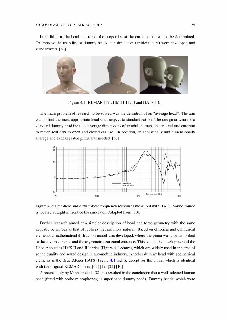
In addition to the head and torso, the properties of the ear canal must also be determined.
To improve the usability of dummy heads, ear simulators (artificial ears) were developed and
standardized. [63]
Figure 4.1: KEMAR [19], HMS III [23] and HATS [10].
The main problem of research to be solved was the definition of an “average head”. The aim
was to find the most appropriate head with respect to standardization. The design criteria for a
standard dummy head included average dimensions of an adult human, an ear canal and eardrum
to match real ears in open and closed ear use. In addition, an acoustically and dimensionally
average and exchangeable pinna was needed. [63]
Figure 4.2: Free-field and diffuse-field frequency responses measured with HATS. Sound source
is located straight in front of the simulator. Adapted from [10].
Further research aimed at a simpler description of head and torso geometry with the same
acoustic behaviour as that of replicas that are more natural. Based on elliptical and cylindrical
elements a mathematical diffraction model was developed, where the pinna was also simplified
to the cavum conchae and the asymmetric ear canal entrance. This lead to the development of the
Head Acoustics HMS II and III series (Figure 4.1 centre), which are widely used in the area of
sound quality and sound design in automobile industry. Another dummy head with geometrical
elements is the Bruel&Kjær HATS (Figure 4.1 right), except for the pinna, which is identical
with the original KEMAR pinna. [63] [19] [23] [10]
A recent study by Minnaar et al. [38] has resulted in the conclusion that a well-selected human
head (fitted with probe microphones) is superior to dummy heads. Dummy heads, which were

CHAPTER 4. OUTER EAR MODELS 26
created from an individual selection process and a copy of an individual human (rather than from
an average) are almost as good as human heads.
4.1.2 Ear canal simulators
The main reason why ear canals are often modelled as straight rigid wall tubes is related to the
wavelength of audible sound waves. The diameter of the ear canal is much smaller than the
wavelength of the highest audible frequencies. The skin on the canal walls has little or no effect
on the acoustics of the canal. Hence, a straight rigid wall tube acts as a good starting point when
building physical ear canal simulators.
Figure 4.3: Cross-section of HATS with the right ear simulator fitted. Adapted from [10].
Since Zwislocki (in 1970) presented his ear-like coupler, many other simulators have ap-
peared, which are supposed to model the acoustical behaviour of the human ear canal. These
devices are important in testing sound sources of high output impedance. [15]
Newer variations of the Zwislocki design have the advantage that they simulate the input-to-
eardrum transfer impedance of the average normal adult ear as well as the input (driving point)
impedance. Thus, a microphone recording made in this type of ear simulator is supposed to
represent the sound pressure that a sound source would have delivered to the eardrum of an
adult listener having a normal ear with average acoustical properties. When used in combination
with a dummy head, the Zwislocki-type ear simulator has numerous applications that include
calibration tests of headphones and hearing aids. [15]
In our research, we used and tested numerous ear canal simulators that to some extent resemble
the Zwislocki-type ear simulator. The simplest version of an ear canal simulator is a straight rigid
wall tube with stiff ‘eardrum’.
This model has been used also in previous studies by [53]. In order to study the effect of
different ear canal shapes, numerous variations of the basic model were developed. The goal
was to develop a simulator and an artificial head that would model the acoustic behaviour of the
human ear, whether blocked or open, as accurately as possible.

CHAPTER 4. OUTER EAR MODELS 27
4.1.3 Tubes as ear canal simulators
For a variety of different modelling and measurement situations, plastic tubes were used to sim-
ulate ear canals. Tubes made of soft plastic material were suitable for studying the effect of
different shapes of the ear canal, as they could be compressed and bended to imitate the structure
of the average human ear canal. Tubes with various inner diameters were tested and used, the
most common diameter used being 8 mm.
The human eardrum is sloping and forms an angle of approximately 40 ◦ with the lower partof the ear canal wall. Most ear canal simulators though, come with an orthogonal eardrum in
relation to the canal. For studies of the effect of the angle between the eardrum and the canal,
two simulators with sloped eardrums were manufactured. The ear canals were made of plastic
tubes with inner diameter of 8 mm and length of 30 mm. The slanted eardrums were made of
aluminium and attached to the tubes. The angles chosen were 25 ◦ and 45 ◦. Small holes in thecentre of the eardrums were drilled for the miniature ‘eardrum’ microphones. In addition, one
otherwise similar device, but with a straight eardrum, was also manufactured.
Figure 4.4: Tubes with slanted ‘eardrums’. A miniature microphone is fitted to the centre of
each eardrum.
4.1.4 Adjustable ear canal simulator (Adecs)
Ear canal simulators, such as the Brüel&Kjær Type 4157 simulator, have been widely used for
ear canal measurements [11]. For better understanding of the acoustic behaviour of the ear canal
we needed to study the frequency responses of a large variety of different sizes of artificial ear
canals. For that purpose the available simulators were not suitable. Therefore, a new device, the
Adjustable ear canal simulator (Adecs), was built.
Figure 4.5: The adjustable ear canal simulator (Adecs) mounted to a microphone stand. In the
picture on the right, the eardrum microphone has been moved to the canal entrance.
The ‘ear canal’ is made of a hard plastic tube with a diameter of 8.5 mm and a total length
of 49 mm. The canal entrance is simply an open round hole. The ‘eardrum’ is made of a

CHAPTER 4. OUTER EAR MODELS 28
movable plastic piston so that the simulator canal length can be adjusted from 0 mm to 39 mm.
A millimetre scale is attached to the side of the canal for easier control of the canal length.
Figure 4.6: A diagram of Adecs. Cross-sections from the front (on the left) and from the side
(on the right).
In the centre of the piston is a round hole, where a miniature Knowles [32] microphone is
fitted. The position of the eardrum microphone is adjustable by hand. It can be located at level
with the eardrum piston or pushed out as far as 57 mm into the canal towards (and outside of)
the canal entrance. The exact position of the microphone is supervised with a millimetre scale at
the back end of the simulator, as can been seen in Figure 4.5.
4.1.5 Multi-adjustable ear canal simulator (Madecs)
A simulator with a stiff eardrum has a frequency response that is significantly different from that
of a human ear. Resonance frequency peaks and antiresonance notches are sharp when measured
with rigid wall simulator, whereas with real ears they are smoother. When the simulator is
blocked with an insert earphone, in the region of 2 kHz, a deep notch is found in the pressure
frequency response when measured at the simulator’s entrance. The notch is caused by sound
wave reflecting from the rigid ‘eardrum’ end of the simulator. The essence of this topic will be
discussed further in Chapter 5.3.
The human eardrum normally softens the mentioned notch by damping the sound wave that
reflects from the drum. The impedance of the eardrum determines the magnitude of the reflecting
wave at different frequencies. For achieving a better analogue with the human ear a new artificial
eardrum was manufactured.
The piston used in Adecs was replaced with a piston made of aluminium and consisting of
the microphone and an adjustable Helmholtz resonator. An opening for the resonator’s neck was
drilled on the membrane and the resonator’s cavity was mounted behind the eardrum piston. A
diagram of the simulator is depicted in Figure 4.7. As with Adecs, the position of the eardrum
piston is adjustable from 0 mm to approximately 40 mm. In addition, the volume of the res-
onator’s cavity can be changed by sliding the back wall of the cavity. In contrast to Adecs, the
position of the eardrum microphone is not adjustable - it is fitted tightly to the eardrum.
The Helmholtz resonator act as damper at the eardrum as some of the sound energy inside the
ear canal is stored in the resonator. Its resonance frequency was initially set to approximately
2 kHz to smoothen the antiresonance notch at the ear canal entrance. The resonance frequency

CHAPTER 4. OUTER EAR MODELS 29
was calculated using equation
f =c
2π
√A
V ·L, (4.1)
where c is the speed of sound, A is the cross sectional area of the neck, V is the volume of the
resonator’s cavity and L is the length of the neck.One important parameter related to resonators such as the ear canal and the Helmholtz res-
onator is the quality factor or Q factor. The quality factor Q for a resonator is the energy stored
in the resonator divided by the energy dissipated in one period. The Q factor determines the
contour of the frequency response curve for a resonator. A low value of Q results in a resonance
spreading over a wide frequency band. At higher values of Q, a resonance will be confined to a
considerable narrower frequency band. [51] [55]
Madecs consists in fact of two resonators, namely the ear canal and the eardrum. The Q factor
of the eardrum affects the impedance but also the Q factor of the ear canal. With a high Q factor
of the eardrum the damping effect of the drum is concentrated around the resonance frequency
of the Helmholtz resonator. A lower Q in the Madecs eardrum would cause a spreading of its
damping effect. In order to spread the damping effect to a larger frequency range, absorbing
material was added inside the resonator’s cavity. The Q factor of the Helmholtz resonator was
thereby lowered. Finally, the wider damping effect resulted in the lowering of the Q factor of the
Madecs ear canal with all ear canal lengths.
Pressure frequency responses with different resonator adjustments are presented in Chapters
5.2 and 5.3.
“Ear canal”
Microphone
Eardrum
piston
Movable
piston Wire
Microphone
Cavity
Neck
Neck
Figure 4.7: A diagram of Madecs. Cross-sections from the front (on the left) and from the side
(on the right).
The simulator was named ‘Multi-adjustable ear canal simulator (Madecs)’ owing to its multi-
ple adjustable parameters.
The IEC 60711 occluded ear simulator uses a somewhat similar system to generate the eardrum
impedance. It applies two Helmholtz resonators and damps the resonators with narrow slits. The
resonators are tuned by adjusting the thickness of shims (at the slits) to control the mid frequency
behaviour of the ear simulator transfer impedance. In the coupler the two resonators are tuned
to approximately 1,300 Hz and 5,000 Hz covering the mid frequency range. [42]

CHAPTER 4. OUTER EAR MODELS 30
4.1.6 Artificial pinnas
The studies of the acoustics of the outer ear called for the introduction of artificial pinnas. An
ear canal simulator without pinna (or head) is suitable only for occluded ear measurements. For
measurements in free field and a listening room, an artificial rubber-made pinna was attached
to the ear canal simulators, as depicted in Figure 4.8. The first pinna used was made of rubber
and it represented an average adult ear, the size and shape of which were close to those of the
KEMAR pinna [19]. Its outer dimensions were 5.8 cm in height and 3.8 cm in width.
Figure 4.8: An artificial pinna attached to Adecs for open ear canal measurements.
Later, when the effects of different shapes and sizes of the pinna were investigated, new pinnas
were constructed. Two larger pinnas were made of hardening plasticine. The first of these
(‘cuplike ear’) had a very deep and large concha, its outer dimensions were 7.5 cm in height and
5 cm in width. The second larger version (‘big ear’) was 8.5 cm in height and 4.5 cm in width,
but the overall shape was close that of an average human pinna. The new pinnas (in Figure 4.9)
were used in measurements together with a dummy head.
Figure 4.9: Artificial pinnas that were used in measurements: ‘cuplike ear’, ‘big ear’ and the
rubber-made ‘normal’ artificial pinna.
4.1.7 Dummy head with adjustable ear canal (Dadec)
With an acoustically realistic ear canal simulator and artificial pinnas ready, the next step in our
research was to build a complete dummy head for acoustic measurements. A manikin head was
modified by replacing the ears with our artificial pinnas and fabricating a torso with dimensions
of an adult human as depicted in Figure 4.10. The pinnas were mounted so that they were
exchangeable and the two ear canal simulators (Adecs and Madecs) were attached in the same
manner.

CHAPTER 4. OUTER EAR MODELS 31
Figure 4.10: Dadec prepared for outdoor measurements.
The dummy head was later used in various free field and listening room measurements, and
it became to be known as Dadec (Dummy head with adjustable ear canals). Henceforward by
default the term ‘Dadec’ refers to the dummy head equipped with the normal size rubber-made
pinna and either Adecs or Madecs as ear canal.
4.2 Computational modelling
Physics-based computational models seek to represent the physical mechanism by which the
external ear transforms the incident sound pressure. In physics-based modelling of the external
ear it is important to take into account that its size is of the same magnitude as the sound wave-
lengths of interest. In addition, the geometry of the external ear is very complex and an analytic
solution to the boundary value problem for this system is probably impossible. Furthermore, the
individual differences are significant and a physical model would have to be individualized to
account for the psychoacoustic consequences of small geometry change. Different models of the
ear canal include various amounts of anatomical details. A sophisticated model can be used for
a large range of sound frequencies and such a model can have good accuracy. [57] [13]
4.2.1 Lumped element and transmission line modelling
One common way to model acoustical systems is to use electrical analogies where the acoustical
system under investigation is turned into lumped electrical elements such as capacitors, resistors
and inductors. Complex mechanical and acoustical systems are modelled with equivalent circuits
consisting of these components. The main benefit from this technique arises from the possibility
to easily change whatever acoustical parameters without laborious physical adjusting. Another
major advantage in this technique is the large number of available software and tools for working
with electrical circuits. [59]

CHAPTER 4. OUTER EAR MODELS 32
Table 4.1: Basic analogous quantities in different physical domains (impedance analogy). q =volume velocity, x = distance, V = volume, φ = magnetic flux and I = inertia [59].
In electrical analogies pressure p in the acoustical domain corresponds to voltage u in theelectric domain, and volume velocity q (acoust.) is equivalent to current i in the electric domain.Impedance is defined as the quotient of voltage and current in the electric domain, whereas in the
acoustical domain impedance is the quotient of pressure and volume velocity. Basic analogous
quantities in different physical domains are presented in Table 4.1.
The lumped element model of electronic circuits makes the simplifying assumption that each
element is a finite-size object in space, and that the wires connecting elements are perfect con-
ductors. The model is valid whenever Lc <<λ, where Lc denotes the characteristic length of
the circuit, and λ denotes the circuit’s operating wavelength. The length of the ear canal is close
to 26 mm, which corresponds to the wavelength at approximately 13 kHz. Electrical analogies
should therefore be used with caution when modelling the ear canal. [59]
The transmission line model assumes that the resistance, capacitance and inductance are dis-
tributed across the whole transmission line. Each circuit element is infinitesimally small. Any
circuit where wave reflections can be significant will usually need to be analysed as distributed
elements.
Insert earphone modelling
Insert type earphones are of special interest in our studies because they block the ear canal
completely and hence change the acoustics of the canal significantly. In order to be able to model
the ear canal when it is blocked with an insert earphone a brief look at earphone modelling is
taken.
Insert earphones (as well as all other types of headphones), which normally use a moving-coil
transducer, can be modelled with simple equivalent circuits.
An example of a schematic view of a moving-coil transducer is depicted in Figure 4.11. The
voice coil, which is in a static magnetic field, is in contact with the membrain. When the current
in the voice coil changes, the magnetic field moves the coil and the membrane. [46] [59]

CHAPTER 4. OUTER EAR MODELS 33
Figure 4.11: Equivalent circuit of a moving coil headphone. Modification from [46] as presented
in [59].
There are three domains that need to be considered in earphone modelling: electrical, mechan-
ical and acoustical. The acoustical components of earphones are volume compliance C, whichis connected to the ground, porous element (R, L in series) and compliant membrane (R, L, C inseries). The analogous quantities in different physical domains are presented in Figure 4.1. The
function of the earphone includes converting the electric sound signals (electric domain) into
membrane movement (mechanical domain) and the movement into sound pressure waves (the
acoustical domain). [59]
In order to apply these modelling steps into one circuit diagram, we need to use transformers
and gyrators. In Figure 4.11 the equivalent circuit of a moving-coil earphone is depicted. The
different domains are modelled separately, but connected with a gyrator (G1) and two transform-
ers (S1 and S2). The gyrator is in the upper part where the electric domain is connected to the
mechanical domain. The transformers connect the mechanical domain to the acoustic domain.
Zload is the acoustic load seen by the earphone.[46] [54]
The quantities in the mechanical domain (F, v) are related to the electric domain (U, I) withequations:
F = B×I l and (4.2)
U = B×vl, (4.3)
where B is magnetic field density and l is the length of the wire in the voice coil. Force, field den-sity, current and velocity are vector quantities but because the vectors are always perpendicular
to each other due to construction of the transducer, the quantities can be considered as scalars.
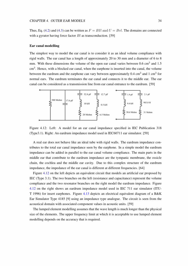
CHAPTER 4. OUTER EAR MODELS 34
Thus, Eq. (4.2) and (4.3) can be written as F = BIl and U = Bvl. The domains are connected
with a gyrator having force factor Bl as transconduction. [59]
Ear canal modelling
The simplest way to model the ear canal is to consider it as an ideal volume compliance with
rigid walls. The ear canal has a length of approximately 20 to 30 mm and a diameter of 6 to 8
mm. With these dimensions the volume of the open ear canal varies between 0.6 cm3 and 1.5
cm3. Hence, with a blocked ear canal, when the earphone is inserted into the canal, the volume
between the eardrum and the earphone can vary between approximately 0.4 cm3 and 1 cm3 for
normal ears. The eardrum terminates the ear canal and connects it to the middle ear. The ear
canal can be considered as a transmission line from ear canal entrance to the eardrum. [59]
Figure 4.12: Left: A model for an ear canal impedance specified in IEC Publication 318
(Type3.1). Right: An eardrum impedance model used in IEC60711 ear simulator. [59]
A real ear does not behave like an ideal tube with rigid walls. The eardrum impedance con-
tributes to the total ear canal impedance seen by the earphone. In a simple model the eardrum
impedance can be added in parallel to the ear canal volume compliance. The main parts in the
middle ear that contribute to the eardrum impedance are the tympanic membrane, the ossicle
chain, the cochlea and the middle ear cavity. Due to this complex structure of the eardrum
impedance, the impedance of the ear canal is different at different frequencies. [64]
Figure 4.12 on the left depicts an equivalent circuit that models an artificial ear proposed by
IEC (Type 3.1). The two branches on the left (resistance and capacitance) represent the volume
compliance and the two resonator branches on the right model the eardrum impedance. Figure
4.12 on the right shows an eardrum impedance model used in IEC 711 ear simulator (ITU-
T 1996) for insert earphones. Figure 4.13 depicts an electrical equivalent diagram of a B&K
Ear Simulator Type 4185 [9] using an impedance type analogue. The circuit is seen from the
acoustical domain with associated component values in acoustic units. [59]
The lumped element modelling assumes that the wave length is much longer than the physical
size of the elements. The upper frequency limit at which it is acceptable to use lumped element
modelling depends on the accuracy that is required.

CHAPTER 4. OUTER EAR MODELS 35
Figure 4.13: Electrical equivalent diagram of a B&K Ear Simulator Type 4185 [9].
Ear canal as transmission line
The sound pressure inside a tube can be calculated using the transmission line model, where the
transmission line is a waveguide. A waveguide is a tube with a small diameter d compared to thewavelength λ of interest. In a waveguide the propagating sound pressure wave is a plane wave.
In the case of a tube with round cross section, the maximum diameter is:
dmax < 0.586λ, (4.4)
The sound pressure in the finite waveguide can be expressed as:
P (ω, x) = iωρ0(P+e−Γx + P−e+Γx) (4.5)
where ω is the angular frequency. P+ is the amplitude of the forward moving wave and P−
is the amplitude of the reflected (returning) wave. P+ and P− are unitless constants. ρ0 is the
density of air, which is approximately 1.2 kg/m3. Γ is the propagation coefficient defined as:
Γ = α+ iβ, (4.6)
where α is the attenuation coefficient and β is the phase change coefficient. In a lossless tube
[62]
e−Γx = e−αxe−iβx, (4.7)
e+Γx = e+αxe+iβx. (4.8)
In a tube with length l and and cross sectional area A, as depicted in Figure 4.14, the pressuresp1 and p2 and volume velocities q1 and q2 in two different locations are:
p1 = iωρ0(P+ + P−), (4.9)
q1 = AΓ(P+ − P−), (4.10)
p2 = iωρ0(P+e−Γl + P−e+Γl), (4.11)
q2 = AΓ(P+e−Γl − P−e+Γl), (4.12)

CHAPTER 4. OUTER EAR MODELS 36
from which the pressure p2 and volume velocity q2 can be solved as:
p2 = p1 cosh(Γl)− Za0q1 sinh(Γl), (4.13)
q2 = − p1Za0
sinh(Γl) + q1 cosh(Γl), (4.14)
where the acoustic impedance of the propagating wave is
Za0 =iωρ0AΓ
. (4.15)
For a lossless transmission line
Za0 =ρ0c
A. (4.16)
This technique will be applied for ear canal modelling in chapter 5.2.6. [62]
Figure 4.14: A transmission line with length l between points of interest. [62]
4.2.2 Estimation of pressure at eardrum
The sound pressure at the eardrum is somewhat difficult to measure. Therefore, several efforts
to estimate the pressure at the eardrum have been made. Estimations are normally based on
measurements along the ear canal and on computational models.
The standing waves inside the ear canal result in different pressure amplitudes in different
parts of the canal. The positioning of the probe tube (or microphone) significantly affects sound
pressure measurement values. Pressure measurements bordering the eardrum are difficult to
obtain because of the sensitivity of the eardrum and its surrounding tissues. It is required that
the introduction of measuring devices into close proximity of the eardrum be made with extreme
caution. Therefore, estimates of eardrum sound pressure are typically made from pressure data
collected at some distance from the drum. [12]
In a study by Sanborn in 1998 [56], the prediction of an electrical analogue model and mea-
surement results were compared. It was found that the measured and predicted responses were
similar from 300 Hz to approximately 6,000 Hz. A major source of error was probe misalign-
ment.
In 1998 Hudde et al [27] presented the reflectance-phase method for estimating the pressure
at the eardrum. It was shown that a good estimation of the pressure can be achieved, even

CHAPTER 4. OUTER EAR MODELS 37
without measuring the input impedance, by only using the minima of the pressure at the ear-
canal entrance. In order to obtain correct estimations, the physical parameters of individual ear
canals have to be determined. They stated that in order to become independent of the properties
of audiometric earphones, the estimation of the eardrum pressure must be based on acoustical
measurements at the entrance of the ear canal. The pressure can be measured with little effort
using a probe tube microphone. To complete the information that can be drawn from acoustical
measurements, the volume velocity must also be measured. The resulting errors of estimation
remained within a limit of 3 dB up to more than 10 kHz.
Figure 4.15: Geometrical descriptors used in the modified horn equation. γ(s) is a general spacecurve that follows the centre of the ear canal and s is the arc length along the curve. At eachpoint s, tangential (s), normal (n) and binormal (b) unit vectors are introduced. The cross sectionthat is defined by the n-b plane has area A(s). [57]
One solution presented by Stinson [57] is to model the ear canal as a curved horn, as in
Figure 4.15. In this case, a modified horn equation can be used for predicting the sound-pressure
distribution along the canal. The trajectory of the canal is represented parametrically by γ(s),where s is the position along the centre axis. The eardrum-end of the canal is set as s = 0. At eachpoint s along the canal, the trajectory is specified by the tangential, normal and binormal unitvectors (s, n and b, respectively). The cross-sectional plane defined by n and b is perpendicularto the centre axis and (bounded by canal walls) forms the cross section of the canal, with area
A(s). Here it is assumed that the sound pressure depends, to first order, only on the parameter s.The spatial variation of sound pressure p is calculated as the solution of the modified horn
equation
d
ds
(A
dp
ds
)+ k2Ap = 0 (4.17)
where k is the wavenumber. [57]

Chapter 5
Measurements
The outer ear plays a significant role in the spectral shaping of sounds before they enter the
inner ear and the nervous system. The pressure frequency responses, or transfer functions, of ear
canals vary greatly. The variation in responses may reach 20 dB at frequencies above 6 kHz. One
of the reasons for different responses in different ears is the variation in the input impedances
of individual human ears. The differences in input impedance are in turn caused by varying ear
canal dimensions and eardrum impedances. [56]
The acoustic behaviour of the outer ear and the ear canal were studied through extensive
measurements with ear canal simulators, a dummy head and human test subjects. The goal was
to learn how the outer ear effects the overall sensation of hearing.
5.1 Measurement equipment and technology
In Chapter 4 we presented a set of new simulators that were manufactured exclusively for our
research. In addition to these physical ear canal models, we needed to build measuring equip-
ment for specific purposes. Furthermore, basic acoustic measurement equipment and software
were needed for measurements on the acoustic behaviour of the outer ear and the ear canal.
5.1.1 Equipment and software
Most of the frequency response measurements were performed using the FuzzMeasure software
versions 3.0.3 and 2.0.11 [58]. The software generates a logarithmic sine sweep and the signal is
sent through the sound card of Apple Macintosh MacBook 4.1 to a loudspeaker or an earphone.
FuzzMeasure records the swept sine through a microphone, which is connected to the sound card
input. The sound pressure frequency and impulse responses are calculated and displayed in the
FuzzMeasure graphic user interface.
Some of the pressure frequency responses were measured using Matlab software. Similar to
FuzzMeasure, the logarithmic sine sweep was played and recorded and the pressure impulse and
frequency responses were obtained thereby.
The pressure transfer function, or frequency response, is obtained by fast Fourier transforma-
tion of (FFT) the impulse response. FFT techniques using sweeps as excitation signals are found
38

CHAPTER 5. MEASUREMENTS 39
Figure 5.1: A pair of earphones with fitted in-ear microphones.
the best choice for transfer function measurements. They are relatively tolerant of time vari-
ance and distortion and choosing a suitable sweep length allows rejection of harmonic distortion
products. By employing a sine sweep signal with exponentially varied frequency, it is possible
to deconvolve simultaneously the linear impulse response of the measured system, and separate
impulse responses for each harmonic distortion order. After the deconvolution of the sampled
response, a sequence of impulse responses appears, clearly separated along the time axis. The
linear frequency response and the corresponding spectra of the distortion orders can be displayed
by FFT analysing each of the impulse responses. Hence, the system is characterised completely
with one, fast and simple measurement. [18]
The Knowles FG-23329 miniature omnidirectional electret condenser microphone was used
in most of the measurements. Its pressure frequency response is adequately flat and it could be
used in small cavities as well as in free field or in a listening room. The length and diameter of the
microphone is only 2.59 mm, which was small enough to fit on the ear canal side of the earphone.
According to our measurements and comparison with a high-precision microphone (B&K 4129),
the frequency response of the FG-23329 is flat from 60 Hz to 10 kHz and reasonably flat from
10 kHz to 17 kHz, where there is a downswing of a few decibels in the microphone’s sensitivity.
Also the Brüel&Kjær 4129 measurement microphone was used in some cases for comparison.
The frequency response graphs presented in this thesis are produced with FuzzMeasure. In the
figures above the graph, the text ‘Frequency Response’ refers to pressure frequency response.
Smoothing is needed to improve readability, and the text inside brackets tells howmuch the graph
has been smoothed. Most smoothing is normally needed with listening room measurements and
least with insert earphone and ear canal simulator measurements. The text ‘Magnitude’ refers
to signal voltage levels (sound pressure level in acoustical domain) compared to the software’s
maximum, which is given the value 0 dB. In some cases the levels have been normalized, in
which case the average level is 0 dB.
5.1.2 Earphone with fitted in-ear microphone (Efim)
For measuring the frequency responses of a blocked ear canal, a special earphone was con-
structed. A Knowles miniature microphone was fitted in front of the transducer port of a Philips
SHN2500 earphone as depicted in Figures 5.1 and 5.2. When the acoustic behaviour of a blocked
ear canal or ear canal simulator was studied, this ‘Earphone with fitted in-ear microphone (Efim)’

CHAPTER 5. MEASUREMENTS 40
was placed at the canal entrance and a sine sweep was excited with the earphone. The sine sweep
was recorded with the fitted miniature microphone.
Figure 5.2: A diagram of Efim. From left to right: View from the side; rubber mould attached to
the earpiece; microphone position depicted from above; cross-section depicting the transducer
and the tube leading from transducer to transducer port.
The microphone was placed far enough from the transducer port to avoid blocking the port too
much as shown in Figure 5.2. In the case of the microphone getting into contact with earwax the
microphone sound port would easily be blocked, which would dilute the microphone’s quality
especially at high frequencies. Therefore, as a preventing measure, the microphone was fitted so
that the transducer port was pointing towards the earphone transducer.
The transfer function from the transducer of Efim to the fitted miniature microphone when
Efim is placed in free field is depicted in Figure 5.3. The strong peak in the frequency response
at 6 kHz is the earphone’s self-resonant frequency peak. This peak is unfortunately very close to
the frequencies where the first half-wave resonance of a blocked ear appears (see Chapter 5.3).
During the mounting of the microphone, the ready-fitted felt at the transducer port was removed
and this made the peak at the resonant frequency somewhat sharper.
Figure 5.3: Transfer function (frequency response) from Efim’s transducer to its microphone in
free field conditions.

CHAPTER 5. MEASUREMENTS 41
5.1.3 Measurement environments
A major part of measurements with open ear canal was made in free field in the large anechoic
chamber of the Department of Signal Processing and Acoustics. A Genelec 1030A active loud-
speaker was placed 2 metres from the point of measurement. A logarithmic sine sweep signal
was played with the loudspeaker via the built-in output of a MacBook laptop. FuzzMeasure
software was normally used to generate the signal and to capture the frequency responses. In
some cases also Matlab software was used for signal generating and recording.
Listening room measurements were performed in the listening room of the Department of
Signal Processing and Acoustics. Its acoustics have been designed to fit the ITU-R BS.116
standard, e.g. the reverberation time of it is constant ≈ 0.3 seconds at a broad frequency region.The same hardware and software as in free field were used in listening room measurements as
well. [49]
With blocked ear canals it was possible to perform measurements in normal quiet room acous-
tics, since the signal-to-noise ratio inside the blocked ear canals was high enough. Hence, most
of the blocked ear canal pressure frequency responses (with simulators and live subjects) were
obtained in a normal office environment.
5.2 Acoustic properties of open ear canal
Quarter wave resonator
The ear canal, closed at the other end by the eardrum, acts as a quarter-wavelength resonator.
The resonance frequencies of an open cylindrical tube, such as the ear canal, are
fn =nc
4(L+ 8r3π )
(5.1)
where n is an odd number (1, 3, 5...), L is the length of the tube, r is the radius of the tube and cis the speed of sound in air (which is approximately 343 metres per second at 20 °C and at sea
level). The resonator produces only odd harmonics and has a fundamental frequency an octave
lower than a tube that is open at both ends. At the resonant frequency and its harmonics, a peak
in the frequency response of the open cylindrical tube appears. These peaks are strongest at the
closed end of the tube and weaken towards the opening of the tube.
From an acoustic point of view a pipe that is open at the other end is longer than its physical
length because of the effect of the mass of attached air. The denominator L + 8r/3π in Eq. (5.1)constitutes the effective, or ‘acoustic’ length of the pipe where 8r/3π = 0.8488r is the ‘endcorrection’. It should be noted that the end corrections depend only slightly on the frequency,
which is not included as a variable in Eq. (5.1). [51] [17]
5.2.1 Frequency response at the ear canal entrance
The head related transfer functions are often measured with a microphone at the ear canal en-
trance, either with a blocked ear canal or with the ear canal left open. With open ear canals

CHAPTER 5. MEASUREMENTS 42
the microphone is pushed a few millimetres into the ear canal and with blocked ear canals the
measurement point is close to the ear canal entrance. [68] [40]
In order to better understand the behaviour of the frequency responses, or HRTF’s, measured
at the ear canal entrance, a set of measurement was performed with various measurement setups
and equipment. A secondary objective was to give us means to assess the usability of the method
of measuring individual HRTF’s from the ear canal entrance.
Adecs in free field
When studying the pressure frequency responses of Adecs, the simulator was mounted to a
microphone stand (as in Figure 4.5) in the anechoic chamber and pointed towards a loudspeaker
at a distance of 2 metres. The frequency responses at different points along the ear canal were
measured using the movable eardrum microphone of the simulator.
Transfer functions from loudspeaker to the Adecs ear canal entrance are depicted in Figure
5.4. Three different canal lengths were used, of which one was zero. The peaks of the resonant
frequencies of the quarter-wave resonators are still visible (in Figure 5.4 around 3, 4, 10 and 12
kHz) when the response is measured exactly at the canal entrance. In the frequency domain,
directly after the peaks follow the anti-resonance notches. The frequencies where these notches
are located correspond to the distance between the measurement point and the eardrum, from
where the reflected sound wave arrives. The existence of both peaks and notches when the
frequency response is measured at the entrance of the ear canal is an indication that the acoustic
entrance of the tube is outside of the physical entrance. This ‘end correction’ phenomenon was
described in the beginning of this chapter. The resonant frequency peaks disappear when the
measurement point is chosen far enough outside of the canal entrance, and only a small anti-
resonance notch remains.
Figure 5.4: Frequency response at the ear canal entrance of Adecs with three different ear canal
lengths measured in free field conditions.
We noticed during our research that when frequency responses are measured at the entrance
of a straight tube ear canal simulator, such as Adecs, the results are practically unsensitive to
the position of the microphone as long as the distance to the eardrum remains the same. In
other words, only the position of the microphone in relation to the length of the canal is signifi-

CHAPTER 5. MEASUREMENTS 43
cant. This is, however, not the case with real ears of human test subjects, as can be found from
literature (e.g. [21]).
Adecs with pinna in free field
The effect of the artificial pinna to the pressure at the ear canal entrance was investigated
with measurements in free field. The pressure frequency responses were measured with Adecs
eardrum microphone with three different ear canal lengths. The effect of only the pinna, without
resonances form the ear canal, can be read from Figure 5.5, where the black line represents the
case where the canal length is set to zero. The pinna notch around 9 - 10 kHz is clearly visible
in all cases. Without the artificial pinna attached, and with ear canal length set to 0 mm, the
pressure frequency response was flat.
Figure 5.5: Frequency response at the ear canal entrance of Adecs when an artificial pinna is
attached to it (only the pinna, as depicted in Figure 4.8). Three different ear canal lengths used
in free field conditions.
The total acoustic length of the ear canal is more than the length of the Adecs canal, since the
concha de facto lengthens the ear canal by approximately 8 mm. In addition, the acoustic length
is more than the physical length due to the end correction phenomena. Hence, the quarter-wave
resonance peak is located at frequency given by Eq. (5.1).
In Figure 5.5, with Adecs canal length 23 mm, the quarter-wave resonance is at approximately
2400 Hz given by
f =343 m/s
4·(0.023 m + 0.008 m + 0.8488·0.005 m) ,
where 0.023 m is the canal length, 0.008 m is the length added by the concha, 0.8448 is the end
correction multiplier and 0.005 m is the radius of the canal entrance of the artificial pinna.
Similarly, in Figure 5.5, the frequency of the antiresonance (3570 Hz) is calculated as
f =343 m/s
4·(0.023 m + 0.001 m),
where the distance from the eardrum to the microphone is 24 mm (23 mm + 1 mm end cor-
rection). This frequency is determined by only the distance from eardrum to the microphone
transducer port.

CHAPTER 5. MEASUREMENTS 44
Dadec in listening room conditions
Similar measurements were performed in listening room conditions using the dummy head
Dadec with Adecs as ear canal. The pressure was measured at a depth of circa 5 mm inside
the Adecs ear canal. The canal entrance of Adecs was circa 5 mm millimetres deeper inside the
head than the canal entrance of the artificial pinna. Hence, the microphone was approximately
10 mm inside the open ear canal of Dadec. The pinna made the total acoustic length of the ear
canal significantly longer than it would have been without the pinna, which moved the fourth-
wave resonance peaks to lower frequencies. The places of the anti-resonance notches, though,
were unaffected by the pinna, since they are affected only by the distance between the eardrum
and the microphone. Naturally, the acoustics of the room made the pressure frequency responses
rugged when compared to responses measured in free field.
Figure 5.6: Responses at the ear canal entrance of Dadec with Adecs as ear canal. Three different
ear canal lengths were used in listening room conditions.
Microphone positioning
When HRTF’s are measured at the entrance of the ear canal, the positioning of the microphone
has a significant effect on the obtained responses. In order to learn more about this fact we
measured the pressure frequency responses in various points at the ear canal entrance of Dadec
in the listening room. Figure 5.7 shows the different positions used in this measurement. A
loudspeaker was placed at a distance of 1.5 metres from the ear canal entrance. The loudspeaker
was pointing towards the ear. The Adecs canal length was set to 14 mm, and the pinna added
approximately 8 mm to the total ear canal length. The differences in the measured pressures are
outstanding as can be seen from Figure 5.8. With the same insertion depth but with different
front-back positions the frequency responses vary greatly from 2.5 kHz upward.
According to Blauert [8] the pressure measured by the microphone depends on where in the
modal resonance the microphone is. Dimensions in these modal resonances are small and even
a slight change in microphone positioning changes the frequency response exceedingly. [34]
These results encourage us to look with extreme caution at pressure frequency response mea-
surements made at the open ear canal entrance.

CHAPTER 5. MEASUREMENTS 45
Figure 5.7: Positions of microphone used in Figures 5.8 and 5.10.
Figure 5.8: Responses at different points at the ear canal entrance. Measurement performed in
listening room conditions using the Dadec with Madecs as ear canal.
Responses at canal entrance of real ears
It is common for HRTF’s to be measured from the ear canal entrance or from a point inside
the ear canal close to the entrance. Also, in earlier studies by e.g. Riikonen et al [53], the
pressure frequency response of the open ear canal has been measured by inserting a subminiature
microphone [32] into the ear canal, the insertion depth being 5 mm from the ear canal entrance.
The goal has been to capture the response at the ear canal entrance and use that response for
determining a target response of an insert type earphone. This frequency response, or transfer
function, is said to represent the natural listening experience. [53]
Within our research, the same set of measurements was repeated first with three subjects
in free field. The Knowles miniature omnidirectional microphone was placed at the subjects’
ear canal entrances and a sine sweep signal was played using a loudspeaker. The speaker was
located at approximately 2 m from the test subject and it was directed so that the subject’s open
ear canal was facing the speaker. To remove the loudspeaker’s and the microphone’s responses
from the result, the measurement recordings have been edited in FuzzMeasure by subtracting
the frequency responses of the microphone and the loudspeaker (in free field) from the measured
ear canal responses. The obtained pressure frequency responses are depicted in Appendix B in
Figures B.1, B.2 and B.3. The differences in the individual ear canal frequency responses were
of great interest as we aimed to better understand the acoustics of the ear canal.
What can be seen from Figures B.1 and B.2 is the quarter-wave resonance of the open ear
canal, which is normally located in the area of 3 kHz for an ear canal with physical length of
26 mm. The acoustic length (with end correction) of such an ear would be circa 29 mm. The

CHAPTER 5. MEASUREMENTS 46
quarter-wave resonant frequency peak is not at all pronounced in the frequency response graph
of Subject 3 (Figure B.3).
What cannot be measured from the ear canal entrance is the spectrum of the sound as it appears
at the eardrum. The variation in sound transmission from the entrance of the ear canal to the
eardrum from subject to subject can for certain frequencies be as much as 20 dB. [20]
5.2.2 Frequency responses along the canal
Responses along the canal: real ears
The frequency responses at different points in the ear canal were also measured using one test
subject. The same setup as above was used with the exception that the responses were measured
with the microphone inserted at different depths into the ear canal. The measured frequency
responses are depicted in Figure 5.9.
Figure 5.9: Responses measured from the open ear canal of Subject 1 with three different mi-
crophone insertion depths inside the ear canal in free field conditions. The measuring points are
3 mm, 6 mm and 10 mm from the ear canal entrance towards the eardrum.
In these measurements a miniature microphone was inserted into the ear canal of the test
subject. With this setup it was impossible to monitor the exact positioning and insertion depth
of the microphone. In addition, the position of the subject’s head was not constant. The used
microphone was omnidirectional, which means that the angle of the microphone in relation to
the ear canal was inconsequential and only the position of the microphone was relevant to the
result.
Even very small variations in the position of the inserted microphone cause great differences
in the measured frequency responses, since the locations (in frequency domain) of notches are
directly dependent of the distance between the microphone and the eardrum. Very close to
the horn-like canal entrance the sound wave is not a simple plane wave, which gives cause to
variations in the frequency response from the overall position of the microphone and not only
the distance between eardrum and microphone.
It is well known that in the ear canal the sound signal already contains all directional infor-
mation that is gathered from the room, torso, head and pinna. The ear canal may alter the sound
differently at different frequencies, but it does so independently of the direction from which the

CHAPTER 5. MEASUREMENTS 47
sound has arrived. Literature from e.g. Møller [40] [39] rest on the assumption that the overall
frequency response does not affect the way sound object locations are perceived and that only
relative differences in frequency response are important. Hence, if we are interested only in the
differences between direction-dependent HRTF’s, a method with a microphone in the ear canal
can be a reliable and functional method. Studies by Griesinger [20], though, suggest that the
individual HRTF’s should be measured at the eardrum even for localization purposes. Measure-
ments from the eardrum are more reliable than those from close to the canal entrance because
of their reproducibility. Varying microphone positioning cause differences between individual
measurements when the measurement point is close to the canal entrance. There differences do
not occur when the measurement point is close to the eardrum.
Frequency responses along the canal: simulators
When the pressure frequency response is measured deep enough inside the ear canal the above
mentioned variations diminish and only the distance to the eardrum is significant. As a demon-
stration of this phenomenon, we measured the frequency responses deep inside the Dadec ear
canal by inserting a microphone into the canal. The microphone was kept at constant distance
from the eardrum, but the horizontal position and elevation was varied. As can be seen from
Figure 5.10, the obtained responses are similar with all four different measurement points.
Hence, if frequency responses are to be measured from the ear canal, it would be recommend-
able to place the microphone deep enough into the canal where the sound wave acts like a plane
wave. A ‘safe’ insertion depth is at least the diameter of the ear canal. In addition, if comparison
between different individuals is to be done, the microphone should be placed at the same dis-
tance from the eardrum of each subject measured, since different insertion depths give different
notch locations.
The position of the eardrum microphone of the adjustable ear canal simulator (Adecs) can be
set to whatever chosen distance from the eardrum towards the ear canal entrance as described in
Chapter 4.1.4. The frequency responses along the Adecs ‘ear canal’ were measured by moving
the microphone tip with 1 mm steps from the eardrum towards the entrance and beyond as
far as 15 mm outside the canal entrance. The effect of the position of the microphone was
Figure 5.10: Effect of microphone position inside the ear canal. Measurement performed in a
listening room using Dadec with Madecs as ear canal.

CHAPTER 5. MEASUREMENTS 48
Figure 5.11: Responses measured in free field along the ear canal of Adecs by adjusting the
position of the microphone. The canal length is 23 mm and the microphone positions are 5, 7, 9,
11 and 13 mm from the ear canal entrance.
investigated in free field conditions with different canal lengths. The loudspeaker was positioned
in front of Adecs at a distance of 2 metres. In Figure 5.11 the responses along the Adecs canal
are depicted. The resonant frequency peaks of the quarter wave resonator remain in the same
positions independent of the microphone position, but the locations of the antiresonance notches
depend on the distance between the eardrum and the microphone.
Figure 5.12: Responses measured in free field along the ‘ear canal’ of Adecs while adjusting the
position of the microphone. The canal length is 23 mm.
In Figure 5.12 the microphone is pushed far enough outside of the canal entrance of Adecs
to allow the peak of the resonant frequency to fade out. The other measurement points are
at the eardrum and at the ear canal entrance. Obviously the terms ‘acoustic length’ and ‘end
correction’ do not imply that at a distance of the end correction outside of the canal, there is
an exact location, where the resonance peak and antiresonance notch disappear. According to
Eq. (5.1), the acoustic length of Adecs is approximately 4 mm more than its physical length. At
a distance of 7 mm from the ear canal entrance, the resonances are still visible though.
A similar study in free field was performed with Adecs when an artificial pinna was attached
to it as depicted in Figure 4.8. The measurement points along the canal were at the eardrum;
11 mm inside the canal; at the entrance and 11 mm outside the canal (inside the concha). The
peak in the resonant frequency at 2.4 kHz remains at a constant position and it is strongest at the
eardrum. In addition, there are no notches at the eardrum. What should also be noticed from

CHAPTER 5. MEASUREMENTS 49
Figure 5.13 is that the resonant frequency peak is visible even when the tip of the microphone is
pushed as far as 11 mm outside of the ear canal. This suggests that the resonant frequency of the
ear canal can be found with measurements from outside the ear canal entrance. The situation is,
however, not that straightforward with live subjects as was discussed in Chapter 5.2.1.
Figure 5.13: Responses measured in free field along the ‘ear canal’ of Adecs by adjusting the
position of the microphone. The canal length is 23 mm and an artificial ear is attached to the
canal entrance.
5.2.3 Frequency response at the eardrum
Adecs in free field
When a sound wave enters a tube that is closed at the other end, the sound pressure has its
maximum at the closed end [17]. Antiresonance notches do not exist at the closed end, as in
other parts of the tube. The pressure peaks of the resonant frequencies of the quarter-wave
resonator tube are however pronounced at the closed end. The Adecs was used to study the
behaviour of the resonant frequency peaks as the length of the ‘ear canal’ changes. In an anechoic
chamber the length of the Adecs canal was adjusted with 1 mm steps from 0 to 30 mm while the
pressure frequency responses were measured with the eardrum microphone. Some examples of
these responses are depicted in Figure 5.14. The location of the quarter-wave resonances can be
calculated with Eq. (5.1).
Figure 5.14: Pressure frequency response at the eardrum of Adecs with different ear canal
lengths in free field conditions.

CHAPTER 5. MEASUREMENTS 50
With a canal length of 24 mm and canal diameter of 8.8 mm, the calculated resonance fre-
quency is at 3.09 kHz, which is close to the measured value 3.17 kHz. If we calculate the acoustic
length based on the resonance frequency, we obtain a length of 23.3 mm for the ‘24 mm’ canal.
9.6 kHz and 16 kHz are the measured frequencies for the second and third resonances. These
too correspond well to Eq. (5.1) as we can calculate these by multiplying the first resonance
frequency with 3 and 5.
Dadec with Adecs in listening room
The custom-made dummy head Dadec was first used for measuring simultaneously the pressure
frequency responses at the eardrum and the ear canal entrance. In listening room conditions, the
Dadec was placed at a distance of 2 metres from a loudspeaker. The eardrum responses were
measured with the Adecs eardrum microphone. An additional miniature microphone was fitted
5 mm inside the ear canal. This location is, however, farther away than 5 mm from the acoustical
entrance of the canal. The concha and the end correction effect cause the ‘real’ entrance to move
outwards by several millimetres. Based on the quarter-wave resonance, in this measurement, the
concha and the end correction added 17 mm to the acoustic length of the ear canal. This result
was invariable with all the different canal lengths (of Adecs) used in this measurement.
The responses were measured with different ear canal lengths with intervals of 1 mm. The
obtained pressure frequency responses at both ends of the tube, with canal length 20 mm is
depicted in Figure 5.15. Additional results can be found in Appendix B in Figures B.5 and
B.6. The responses are similar from low frequencies up to the first fourth-wave resonance. The
pressure at the eardrum then drops gradually towards higher frequencies. The pressure at the
entrance, though, drops rapidly towards the first antiresonance notch. The peak at the first fourth-
wave resonance and the notch at the antiresonance are both very sharp. This characteristics
gave reason to develop an eardrum for the simulator that would behave more like a real human
eardrum, which softens the resonance and antiresonance peaks significantly.
Figure 5.15: Frequency response at ear canal entrance and the eardrum measured using Dadec
with Adecs as ear canal in listening room conditions.

CHAPTER 5. MEASUREMENTS 51
Dadec with Madecs in listening room
The new multi-adjustable ear canal simulator (Madecs), with a damped eardrum, was manufac-
tured as we wanted to obtain frequency responses that are close to those measured with human
subjects. When finished, the Madecs was fitted to the dummy head Dadec. To investigate re-
sponses at the eardrum of Dadec with Madecs as ear canal in listening room acoustics a new set
of measurements was performed.
Figure 5.16: Responses with various ear canal lengths measured at the eardrum of Dadec (with
Madecs as ear canal) in the listening room.
The Dadec was placed directly facing (θ = 0) a loudspeaker at a distance of 180 cm. The
pressure frequency responses at the eardrum are depicted in Figure 5.16. Compared to previous
measurements with Adecs, the quarter-wave resonant frequency peaks are significantly softer.
This effect is caused by the damped eardrum of Madecs.
During the measurement two different ear canal simulators were attached to the Dadec, of
which Madecs was the primary simulator, whereas Adecs was used mainly for reasons of com-
parison with Madecs but also for measuring the differences between pinna’s of different sizes.
The pressure frequency responses were recorded with the eardrum microphones of Adecs and
Madecs, which were sequentially attached to Dadec. Responses obtained using the Adecs as ear
canal are depicted in Figure 5.17.
Figure 5.17: Dadec (with Adecs as ear canal) in listening room acoustics with different ear canal
lengths. Frequency responses measured at the eardrum.

CHAPTER 5. MEASUREMENTS 52
Dadec in free field
The Dadec was also used for studies of the frequency response at the eardrum in free field con-
ditions. The impedance of Madecs was adjusted to significantly damp the frequencies between
1 kHz and 3.5 kHz before mounting the simulator to the dummy head. In an anechoic cham-
ber, the angle between the head’s median plane and the loudspeaker (azimuth angle) was set to
30 ◦. Again, the influence of the canal length on the responses at the eardrum was measured.
The peak of the quarter-wave resonance frequency is apparent, but there is another peaking with
constant frequency at 4.8 kHz, which is caused by the boosting effect of the pinna, as can be
observed from Figure 5.18. Compared to responses in a listening room, the effect of the pinna
and the ear canal are more pronounced in free field measurements. When no reflections exist,
other than those of the head and pinna, the effect of individual dimensional variations become
more apparent.
Figure 5.18: Dadec with Madecs as ear canal, in free field, with different ear canal lengths. The
head is facing the loudspeaker with an azimuth angle of 30 ◦. Frequency responses measured atthe eardrum.
Measurements at the human eardrum
The transfer function from the loudspeaker to the eardrums of a live subject (Subject 1) with
one sound source direction was measured. The setup was identical to that of the preceding
measurements setup with Dadec in listening room conditions, only that responses from both left
and right ears were measured. A loudspeaker was placed at a distance of 1.8 metres form the
listener (with azimuth angle of 0 ◦). A miniature microphone was inserted into the ear canal andmoved very close to the eardrum, without touching it (the test subject performed the insertion
by his own hands). The position of the microphone was kept stable while the logarithmic sine
sweep was played with the loudspeaker. Pressure frequency responses from the eardrum were
thus obtained using the inserted microphone.
The obtained responses in Figure 5.19 show the quarter-wave resonance at approximately 2.2
kHz with both ears. The pressure then drops uniformly. The effect of the pinna increases the
pressure between 3 kHz and 7 kHz and the lowers it between 8 kHz and 10 kHz. The differences
between the two ears at frequencies above 10 kHz are related to the curvature and overall shape

CHAPTER 5. MEASUREMENTS 53
Figure 5.19: Frequency responses measured close to the eardrums of Subject 1 in listening room
conditions.
of the subject’s ear canals, where the more curved right ear canal causes the pressure to drop
more compared to the straighter left ear.
The responses measured at the eardrum of Subject 1 Figure 5.19 are much like those measured
with Dadec (Figure 5.25) with the samemeasurement setup. The Dadec withMadecs as ear canal
hence models the human peripheral hearing fairly accurately.
5.2.4 Effect of different outer ear shapes
As mentioned in previous chapters, the length of the ear canal has a strong effect on the pressure
frequency response at the eardrum, as well as at the ear canal entrance. The other parts of the
outer ear also have individual differences. A large amount of measurements was performed to
study as to how significant the other physical variations are to the frequency responses.
Effect of the shape of the pinna
Three different fabricated pinnas were attached to Dadec with Adecs as ear canal in order to
investigate the effect they had to the pressure at the eardrum. In addition to the rubber-made
pinna used in most measurements, two larger pinnas (big ear and cuplike ear) were used (see
Chapter 4.1.6). In a listening room, a loudspeaker was placed in front of the Dadec (azimuth
angle 0 ◦), at a distance of 1.8 metres. The pressure at the eardrum was measured while a sinesweep signal was played with the loudspeaker. The effect of the two large ears were measured
using an Adecs canal length of 22 mm. Due to different attaching mechanisms, the acoustic
length of the pinna plus ear canal was shorter with the larger pinnas compared to the small
rubber pinna. Therefore, to obtain the same acoustic length with all ears, the rubber pinna was
measured using a Adecs canal length of 12 mm (instead of 22 mm).
The frequency response curves in Figure 5.20 show that below 2 kHz the larger pinnas increase
the pressure at the eardrum when compared to the smallest pinna. The pinna notch is clearest
with the small ‘rubber ear’. The overall differences in the obtained frequency responses are not
striking considering the huge differences in the physical sizes of the pinnas. The differences
between sizes and shapes of normal human pinnas are much smaller.

CHAPTER 5. MEASUREMENTS 54
Figure 5.20: The effect of the size and shape of the pinna. Three different fabricated pinnas
attached to Dadec with Adecs as ear canal. Responses measured from the eardrum of Adecs.
Effect of canal shape
Ear canals are often modelled as straight rigid wall tubes. Since the wavelengths of audible
sound waves are greater than the diameter of the ear canal, we may consider the sound waves
travelling only in the direction of the canal. No standing waves arise in cross-canal direction.
The situation does not change much if the canal is slightly bended along its length - the sound
wave ‘sees’ the canal as a straight tube and propagates towards the eardrum despite the curvature.
The shape of the canal has, however, influence on the frequency response of the canal.
One of the most common reasons for different frequency responses of open ear canals is
variable shape of the ear canal entrance. We define these variation as being related to the effect
of the pinna and not the ear canal.
The effect of ear canal curvature was studied by measuring responses from the eardrum of
different tubes in free field. A tube with length of 30 mm and diameter of 8 mm was first
compressed in the middle part and the obtained response was compared with that of the un-
compressed version. The compressing effectively decreased the canal diameter to 6 mm in the
middle part of the canal. The effect of this procedure is depicted in Figure 5.21. Below 7 kHz,
the compressing boosts the sound, whereas from 7 kHz to 13 kHz the effect is opposite.
Figure 5.21: The effect of the shape of the ear canal. Responses measured at the eardrum in free
field conditions with open ear canal.

CHAPTER 5. MEASUREMENTS 55
In addition, the mentioned straight tube was bended to form a sheer 70 ◦ angle in the middlepart. The bending caused also a partial blocking halfway of the canal. There are hardly any ear
canals with a shape of this kind, but the effect of a violent deformation such as this gives further
understanding of the acoustic behaviour of the ear canal. The frequency responses obtained
from the eardrums of the straight and bended tubes are depicted in Figure 5.22. The response
curves have nothing in common above 2 kHz and there is a remarkable attenuation from 5.5 kHz
upwards. As a general interpretation one might conclude that the more curved the ear canal the
more it attenuates high frequencies.
Figure 5.22: The effect of the shape of the ear canal. A straight tube and the same tube bended
in the middle produce very dissimilar frequency responses. Responses measured in free field.
The tubes have equal length (30 mm) and equal diameter (8 mm).
Figure 5.23: The effect of the angle of the eardrum in relation to the ear canal. The frequency
responses of three tubes with different angles of the ear canal measured in free field conditions.
As a third dimensional property the angle of the eardrum in relation to the ear canal was
investigated. For this study three similar tubes with three different eardrum angels were used
(0 ◦, 25 ◦ and 45 ◦), of which the tube with eardrum angle 45 ◦ represents the normal human earcanal. The tubes had equal length (30 mm) and equal diameter (8 mm). All of the eardrums were
made of aluminium and they had a miniature microphone fitted into the centre.
The pressure frequency responses at the eardrums of these simulators were measured in free
field. The obtained responses are depicted in Figure 5.23. The difference in the responses
between the ‘normal’ (45 ◦) eardrum and the straight (0 ◦) drum are significant above 2.2 kHz.Hence, in the development of ear canal simulators this property should be taken into account.

CHAPTER 5. MEASUREMENTS 56
Effect of the head
The size of the head is an important factor in sound source localization as it determines the inter-
aural time difference. The effect of the size and shape of the head to the HRTF was investigated
with measurements in listening room conditions. The frequency responses from the ear canal
entrance and the eardrum of a Dadec with Adecs as ear canal were measured, while the ‘shape’
of the head was altered. First, we studied the effect of added reflecting objects. Compared to the
‘normal head’ the altered version had a book on top of the head, which acted as a reflector. The
loudspeaker was placed at a distance of two metres from Dadec with an azimuth angle of 30 ◦.The measured frequency responses in Figure B.4 (Appendix B) show that the added reflecting
object had little effect on the pressure at both the ear canal entrance and at the eardrum. The
variations related to the pinna, as discussed above, are significantly more pronounced.
In addition, the effect of a big cap with fillings, which in practice increased the diameter of
the head by three centimetres, was measured. The cap was placed deep enough to cover the
eyes of Dadec. In a listening room, Dadec was first facing the loudspeaker, an in the second
measurement, the head was turned to a lateral angle of 90 ◦. As can be observed from Figure
5.24, once again, the variations had little effect on the frequency responses measured at the
eardrum.
A study by Riederer [52] showed somewhat similar results, when the effect of added head-
pieces was investigated. With a baseball cap on top of a dummy head and with azimuth angles
near the (contralateral) interaural axis (60 ◦ - 120 ◦) only moderate effects were found. Reflect-ing objects around the head are an important factor as to direction-dependent HRTF’s. In our
research though, the focus was on direction-independent spectral shaping characteristic of the
outer ear.
Figure 5.24: In listening room conditions, the responses measured first with Dadec wearing a
cap with fillings and then without the cap. Frequency responses measured at the eardrum with a
canal length (Madecs) of 7 mm. Two azimuth sound source angles (from the side and from the
front) were used.
From these results we conclude that of all the different properties of the outer ear and the head,
the shape and length of the ear canal are the most important factors in determining the pressure
frequency responses at the ear canal entrance and at the eardrum.

CHAPTER 5. MEASUREMENTS 57
5.2.5 Effect of drum impedance
The eardrum is not a rigid straight wall at the end of the ear canal. It participates in the shaping
of the pressure frequency response of the ear canal in a complex way. The effect of the eardrum
was studied using simulators and live subjects.
Simulator eardrums
With the unblocked ear canal, in the listening room, the effects of variable eardrum impedances
were studied. The comparison was made between Adecs, which has an undamped eardrum (see:
4.1.4) and Madecs, with a damped eardrum (see: 4.1.5). Each simulator was mounted to Dadec
consecutively.
Comparison between the frequency responses of the two different ear canal simulators when
they are attached to Dadec in similar listening room environments is shown in Figure 5.25. There
is a significant difference in the responses measured with each of the eardrum microphones. The
damping effect of the Madecs eardrum is clear at the resonant frequencies of the ear canal, where
the eardrum attenuates the peak of the resonant frequency by 6 to 10 dB. The damping is not at
all significant at other frequencies, hence the eardrum decreases the Q factor of the oscillating
ear canal.
The responses are measured at the eardrums of both simulators when the measurement signals
were played with a loudspeaker at a distance of 180 cm and azimuth angle of 0 ◦ in a listeningroom.
Figure 5.25: The effect of the eardrum. Responses measured with the eardrum microphones of
Adecs and Madecs when mounted to Dadec in the listening room. Canal lengths set to 10 mm
and 22 mm.
Real eardrums
Numerous studies have been performed to determine the impedance of the human eardrum.
Measuring the impedance of the human eardrum is not an easy task and means to change the
impedance are limited.
The stapedius reflex changes the impedance as the malleus pulls the eardrum inwards and
makes the drum stiffer. Another way to stiffen the eardrum is to add pressure into the tympanic

CHAPTER 5. MEASUREMENTS 58
cavity. Blowing air from the lungs into the nasal cavity, and simultaneously blocking the nostrils,
causes the additional pressure to expand from the nasal cavity to the tympanic cavity through the
Eustachian tube. This pressure pushes the eardrum outwards and stiffens it significantly.
Figure 5.26: Frequency responses at the eardrum when measured in normal circumstances and
with additional pressure in the tympanic cavity. The response is measured from the left ear with
azimuth angle 0 ◦ in listening room conditions.
The effect of the impedance of the human eardrum to the frequency response measured in
front of it was studied. The responses at the eardrum were measured in normal circumstances,
and then with additional pressure in the tympanic cavity. A miniature microphone was inserted
into the ear canal of a human test subject and moved very close to the eardrum. The frequency
responses were measured from both ears of Subject 1 in a listening room. The test was performed
with sound source azimuth angles 90 ◦ and 0 ◦ for both ears, in the listening room, and with aloudspeaker approximately 1.5 metres from the ear. The responses from the left ear are depicted
in Figure 5.26
Figure 5.27: Difference between frequency responses at the eardrum when measured in normal
circumstances and with additional pressure in the tympanic cavity. Red curve represents the
right ear with azimuth angle 90 ◦ and the black curve represents the left ear with azimuth angle0 ◦.
The differences in the obtained frequency responses are depicted in Figure 5.27. The pressur-
ized tympanic cavity raises the Q factor of of the ear canal and amplifies the first quarter-wave
resonance peaks by 6 dB. It might be worth mentioning, that the difference is the same as when
Adecs and Madecs eardrums were compared (see Chapter 5.2.5 and Figure 5.25). Hence, the

CHAPTER 5. MEASUREMENTS 59
stiffened human eardrum behaves much like a rigid ear canal termination and at the same time,
the damped eardrum of Madecs behaves much like a normal human eardrum.
5.2.6 A computational model
As discussed in Chapter 4.2.1, the acoustic behaviour of the ear canal can be modelled using
lumped elements and transmission line models. In order to compare obtained measurements with
a computational model the Adecs was modelled based on its physical parameters. The modelling
was made with Matlab and it consisted of a straight rigid wall tube with a rigid eardrum. The
length of the tube was set to 23 mm and the diameter to 8.5 mm. The impedance of the eardrum
was set to 4× 10⁸ Ω, which represents a purely resistive impedance. The frequency responses atthe canal entrance and at the eardrumwere calculated by first modelling the ear canal as a lossless
transmission line using the Equations from (4.5) to (4.16). The ear canal entrance quantities were
determined, which were used to calculate the canal entrance to membrane pressure transmission.
The loudspeaker together with the canal entrance were modelled as a sound source with radiation
impedance, and the source to canal entrance pressure transmission was determined. Thereby it
was possible to calculate the normalized canal entrance pressure and the normalized membrane
pressure. The resulting frequency response curves are depicted in Figure 5.28. [31]
Figure 5.28: Computational ear canal model with canal length of 23 mm in free field. The blue
line is the computed response from the canal entrance and the red line is the computed eardrum
response.
The modelled responses are very similar to those measured with open Adecs in free field. The
free field response curves were however more rugged compared to the computational model. An
additional measurement with Adecs in free field was performed in order to obtain as smooth
response curves as possible. By averaging several consecutive measurement sweeps and sub-
tracting the microphone and loudspeaker frequency responses from the results, fairly smooth
response curves were obtained as depicted in Figure 5.29. It should be noted that no additional
smoothing has been applied to Figure 5.29. As presented in Chapter 5.1.1, most of the response
curves from open ears or simulators in this work have been smoothened in FuzzMeasure.

CHAPTER 5. MEASUREMENTS 60
Figure 5.29: Adecs with canal length of 23 mm measured in free field. The blue line is the
response from the canal entrance and the red line is the eardrum response.
The used computational model was very accurate. The modelled and the measured frequency
responses are identical except for the magnitude of the peaks and notches, where there are dif-
ferences of a few decibels.
5.3 Acoustic properties of blocked ear canal
Compared to normal listening conditions with unblocked ear canal, the acoustic behaviour of the
ear canal is very different when it is blocked with e.g. an insert earphone. All of the outer parts
of the auditory system act together to form the total transfer function when the signal is played
with a loudspeaker. In a listening room, with the ear canal left open, also the acoustics of the
room is shaping the frequency response of the system, that is, shaping the transfer function from
loudspeaker to eardrum. When listening to e.g. music with an insert earphone the effects of the
head, shoulders, pinna and concha are cancelled and only the acoustic properties of the ear canal
are of significance. Nevertheless, the outer parts of the outer ear are important in shaping the
way we are used to hearing external sound sources, and they should therefore not be completely
forgotten when contemplating the acoustics of the occluded ear canal.
The behaviour of the blocked ear canal was studied through extensive measurements with both
simulators and human test subjects. One of the most important characteristics of the ear canal
is its length, the effect of which was in the centre of our research. In addition, the effect of the
impedance of the eardrum was studied with simulators and a human test subject. Furthermore,
the effect of ear canal curvature was investigated briefly.
An important device used was the custom-made earphone with fitted in-ear microphone, which
was presented in Chapter 5.1.2. Earlier studies on the behaviour of the blocked ear canal have
been made mostly related to fitting of hearing aid apparatus (see [15] and [56]). The goal of
our research was to improve our knowledge of the behaviour of the ear canal when an insert
earphone is used for e.g. music listening.

CHAPTER 5. MEASUREMENTS 61
Half-wave resonator
In Chapter 5.2 we discussed the properties of the open ear canal and concluded that it acts like
a quarter-wave resonator. The resonant frequencies of the open ear canal are more or less pro-
nounced depending on room acoustics, location of the sound source and the shapes of the pinna
and the ear canal. The pressure maximum is at the eardrum and there is a pressure minimum at
the acoustic entrance of the ear canal, as presented in Chapter 5.2.2. The sound pressure level
at the eardrum is highest around the quarter-wave resonant frequency in both free field and a
listening room and with different angles between the head and the loudspeaker.
Figure 5.30: A tube closed at both ends is a half-wave resonator.
An ear canal blocked at each end could by intuition be modelled as a tube closed at both
ends. E. Vente concluded in 1932, that if a tube is blocked at both ends, symmetry is restored
with opportunity for vibrations in the complete harmonic series [66]. In consequence, the canal
would also behave as a half-wave resonator when the canal entrance is blocked. This would
most certainly be true if the ear canal was blocked with a rigid plug and the eardrum was stiff as
well. When we study the behaviour of the blocked ear canal, the ear canal entrance is normally
blocked with an earphone or a hearing aid. Hearing aids and earphones are not rigid plugs, but
instead they have finite acoustic impedances.
A brief investigation was conducted in order to clarify the half-wave resonator issue. First, two
rigid wall plastic tubes with diameter of 8.5 mm and lengths of 25 mm and 34 mm were blocked
at both ends with stiff plugs. The tubes were then placed in front of a loudspeaker and a sine
sweep was played. The amount of conduction through the plastic walls was enough to produce
standing waves inside the tubes. The frequency responses inside the tubes were measured from
one end of the tube using the piston (eardrum) microphone of Adecs. This measurement showed
that indeed, the tube behaved as half-wave resonator as can be observed from Figure 5.30. The
resonant frequencies are
fn =nc
2L(5.2)
where n is a positive integer (1, 2, 3...) representing the resonance node, L is the length of thetube, r is the radius of the tube and c is the speed of sound in air (which is approximately 343metres per second at 20 °C and at sea level). With a canal length of 34 mm, this equation gives
resonant frequencies at 5 kHz, 10 kHz and 15 kHz, which are very close to the results obtained
from the measurements.

CHAPTER 5. MEASUREMENTS 62
Figure 5.31: Diagram of measurement setup where Efim is fitted to Adecs and the eardrum
microphone is moved towards the earphone.
A similar test was made with an earphone (Efim) blocking the tube at the other end as depicted
in Figure 5.31. The system did not behave similarly to the tube blocked at both ends as can be
seen from Figure B.7 in Appendix B. The resonance of the earphone (around 6 kHz) appears
as an additional peak in the frequency response. Secondly, the earphone end of the tube is not
a straight termination, instead there are several surfaces at different locations from where the
sound pressure wave can reflect. Thus, an ear canal blocked with an insert earphone does have
some of the characteristics of a half-wave resonator, but it is not purely that. The impedances of
both the earphone and the eardrum should be taken into account.
With a 67 cm long tube, though, the half-wave resonator characteristics are clearer. The
system with Efim blocking the entrance of the tube has resonance frequency peaks at locations
that can be calculated with Eq. (5.2), as Figure B.8 in Appendix B shows.
During our research, several measurements were performed with Efim mounted to an ear
canal simulator and the pressure frequency responses were captured with the in-ear microphone
of Efim. These measurements showed an antiresonance notch around 2-3 kHz, as mentioned
earlier in Chapter 4.1.5. A half-wave resonator tube has an quarter-wave antiresonance at
fn =nc
4L(5.3)
where n is an odd number (1, 3, 5...), c is the speed of sound and L is the length of the tube.The antiresonances in the frequency responses measured with Efim were not in accordance with
this equation. The measured antiresonances were at lower frequencies than would have been
expected.
Figure 5.32: Responses measured at various distances from Efim along the Adecs ear canal.
A clarifying additional measurement was performed to study this phenomenon. The measure-
ment setup is depicted in Figure 5.31. The eardrum microphone of Adecs was moved gradually

CHAPTER 5. MEASUREMENTS 63
to close proximity with the Efim in-ear microphone. The Adecs ear canal was adjusted to 20
mm. A sine sweep signal was played with the Efim and the pressure frequency responses were
measured with the eardrum (probe) microphone. Figure 5.32 shows how at a distance of 6 mm
from the earphone, the antiresonances behave almost according to Eq. (5.3). Very close to the
earphone and at the location of the in-ear microphone (Efim), though, the antiresonances shift to
lower frequencies and their locations cannot be calculated with the said equation.
Closer to the eardrum end of the simulator, the locations of the antiresonance notches depend
only on the distance from the measurement point to the eardrum, as long as the canal width
remains constant. This was the case also with the open ear canal as discussed in Chapter 5.2.2.
5.3.1 Frequency responses of blocked ear canal simulators
The pressure frequency responses of Adecs and Madecs, when measured with their eardrum
microphones and the in-ear microphone of Efim, were in the centre of our research. Similar to
the measurements with the open ear canal, the effect of the canal length was studied making
good use of the adjustable simulators.
The first measurements with Adecs and Efimwere performed with the setup depicted in Figure
5.33. The length of the canal was adjusted with 1 mm steps from 5 mm (minimum) to 40 mm.
A sine sweep was played with Efim and the frequency responses were measured with both the
Adecs eardrum microphone and the Efim in-ear microphone. In Figure 5.34 the responses from
Adecs with a 26 mm ear canal are depicted. The graph shows the antiresonance notch at approx-
imately 2 kHz at the earphone microphone. The first half-wave resonance is at approximately
7.5 kHz, which can be calculated using Eq. (5.2):
f =343 m/s
2·(0.026 m− 0.0035 m)= 7622 Hz,
where the 3.5 mm subtraction comes from the insertion depth of Efim, which is normally be-
tween 3 and 4 mm. The peak at approximately 5.8 kHz is caused by the Efim’s self-resonant
frequency.
Figure 5.33: Diagram of measurement setup where Efim is fitted to Adecs and the length of the
canal is adjusted by moving the eardrum piston.
A similar set of measurements was performed with Madecs. The length of the simulator’s
canal was adjusted as frequency responses were measured with the eardrum microphone and the
in-ear microphone of Efim. The eardrum of Madecs is significantly damped, which smoothens
the antiresonance notch around 2 kHz, as can be seen from Figure 5.35. In Figure 5.36 responses
at the eardrum were measured using different canal lengths. The curves move in frequency
domain in unison with the varying canal length.
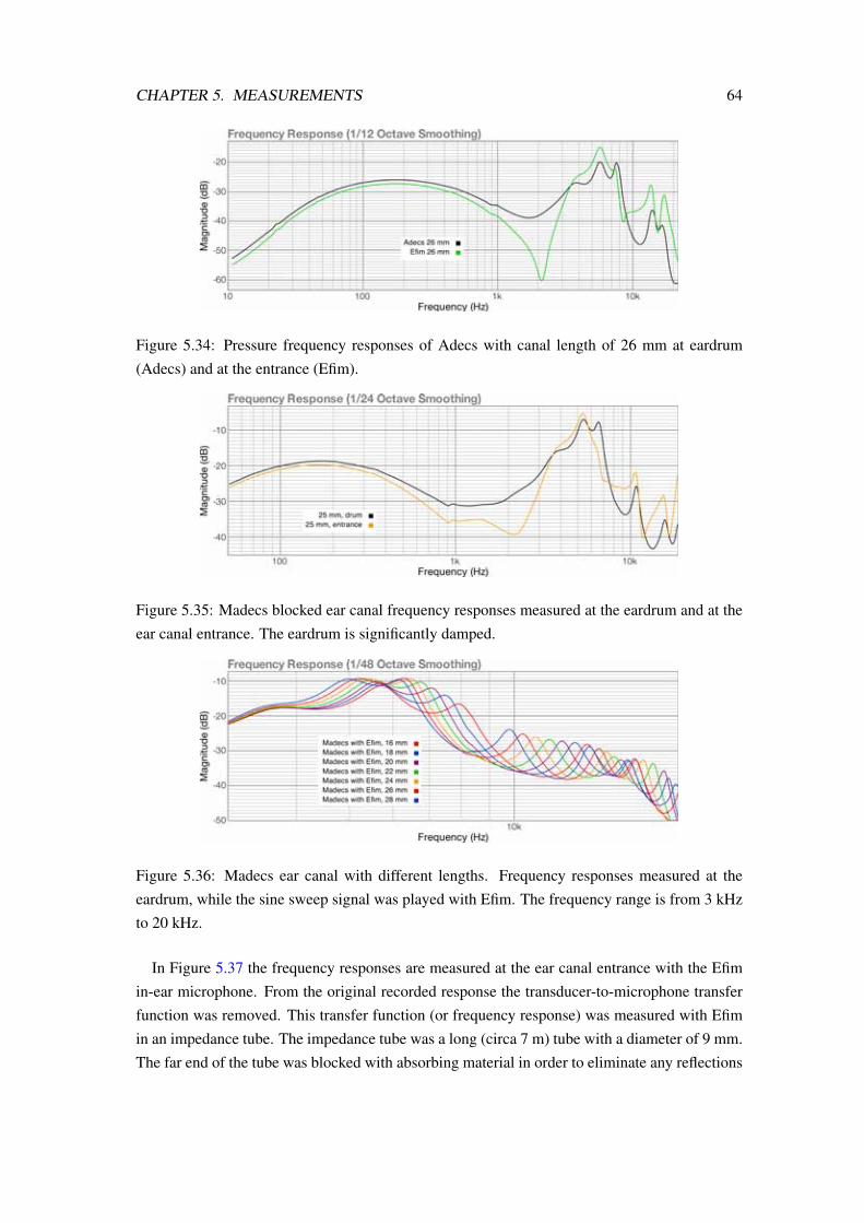
CHAPTER 5. MEASUREMENTS 64
Figure 5.34: Pressure frequency responses of Adecs with canal length of 26 mm at eardrum
(Adecs) and at the entrance (Efim).
Figure 5.35: Madecs blocked ear canal frequency responses measured at the eardrum and at the
ear canal entrance. The eardrum is significantly damped.
Figure 5.36: Madecs ear canal with different lengths. Frequency responses measured at the
eardrum, while the sine sweep signal was played with Efim. The frequency range is from 3 kHz
to 20 kHz.
In Figure 5.37 the frequency responses are measured at the ear canal entrance with the Efim
in-ear microphone. From the original recorded response the transducer-to-microphone transfer
function was removed. This transfer function (or frequency response) was measured with Efim
in an impedance tube. The impedance tube was a long (circa 7 m) tube with a diameter of 9 mm.
The far end of the tube was blocked with absorbing material in order to eliminate any reflections

CHAPTER 5. MEASUREMENTS 65
back towards Efim. The transfer function from the transducer to the microphone was thereby
obtained.
The remaining response in Figure 5.37 should hence be that of the ear canal only. Efim’s
self-resonant frequency peak is, however, visible after the deconvolution. The magnitude and
location of the self-resonant frequency peak changes slightly when the length of the ear canal
changes, which is clearly visible in Figure B.9. This effect is caused by the place shifting notches
around the self-resonant frequency.
The ear canal’s resonance frequency peaks change place distinctly in unison with the changing
length of the ear canal. These peaks are pronounced in frequencies around and above 10 kHz,
as can be seen from Figure 5.37. The peaks move towards higher frequencies when the canal
shortens.
Figure 5.37: Dadec blocked ear canal responses measured at the ear canal entrance, with two
different canal lengths.
5.3.2 Frequency responses of human ears
With the Efim it was easy to measure the pressure frequency responses from real ears. The test
subjects were asked to place the earphone at the ear canal entrance. Then a sine sweep was played
with the Efim, and the frequency response from inside the canal was measured with the in-ear
microphone. Eight test subjects participated in these measurements, both ears of which were
measured. The differences between individuals were significant, and in addition, the differences
between right and left ears were interestingly outstanding with some of the subjects.
The responses from measurements with Subjects from 1 to 8 are depicted in Figures 5.38,
5.39, 5.40, 5.46 and in Appendix B in Figures B.10, B.11, B.12 and B.13. The left and right ear
canals of Subject 6 (Figure 5.38) are remarkably similar, as there is no difference between the
measured responses, whereas the canals of Subject 3 have prominent differences between each
other. The lengths of the canals of Subject 5 (Figure 5.40) seem to be different, since the first
half-wave resonance peaks are located at 7.3 kHz (right) and 8.3 kHz (left). Applying Eq. (5.2),
the lengths of the ear canals of Subject 5 would be close to 24 mm (right) and 21 mm (left). This
‘length’ is the distance from the earphone to the eardrum, and it does not take into account the
earphone insertion depth.

CHAPTER 5. MEASUREMENTS 66
Figure 5.38: Ear canal frequency response measured at the canal entrance of Subject 6. Sine
sweep played with Efim and response recorded with Efim’s in-ear microphone.
Figure 5.39: Ear canal frequency response measured at the left canal entrance of Subject 3. Sine
sweep played with Efim and response recorded with Efim’s in-ear microphone.
Figure 5.40: Ear canal frequency response measured at the left canal entrance of Subject 5. Sine
sweep played with Efim and response recorded with Efim’s in-ear microphone.
The responses obtained from real ears showed similarities with those measured with Efim
using Adecs and Madecs. As one example of this, Figure 5.41 shows the responses measured
with Dadec (with Madecs as ear canal) and the left ear of Subject 2. In this example, the ear
canal of Madecs was set to 22 mm upon which the pinna (or the concha) of Dadec adds a few
millimetres. Hence, the total ear canal length of Dadec, in this case, was approximately 28 mm.

CHAPTER 5. MEASUREMENTS 67
Figure 5.41: Ear canal frequency response measured at the left ear canal entrance of Subject 3
compared with similar measurement from Dadec.
5.3.3 Effect of eardrum impedance
Madecs with different eardrum impedances
The simulator with damped eardrum (Madecs) was built to copy the acoustic behaviour of a
real ear canal as accurately as possible, including the impedance of the eardrum. The effect of
the eardrum is remarkable especially in situations where an insert earphone is the sound source.
The impedance of the eardrum determines the Q factor of the half-wave resonator, formed by
the blocked ear canal. With a stiff eardrum, the antiresonance peak in the frequency response
around 2 kHz is very sharp when compared to corresponding peak in the responses from real
ears. The impedance of a rigid eardrum is high at all frequencies and the Q factor of the ear
canal resonator is therefore also high.
Figure 5.42: Madecs blocked ear canal frequency responses with different eardrum impedances.
The Helmholtz resonator at the eardrum of Madecs is adjustable as to the resonance fre-
quency and the amount of damping as discussed in Chapter 4.1.5. Madecs was tuned to copy
the acoustical behaviour of the human ear canal when a sine sweep is activated with Efim and
the frequency response is measured with Efim’s in-ear microphone. In Figure 5.42 four different
responses with different resonator settings are depicted. The red curve is the response when the
Helmholtz resonator is undamped. Adding absorbing material into the resonator cavity dampens
the resonance and spreads the damping effect of the resonator in frequency domain. The blue
curve is the response with slightly damped Helmholtz resonator. The black curve represents a

CHAPTER 5. MEASUREMENTS 68
setting, where the damping is similar to that of many human eardrums when the response is
measured with Efim.
Figure 5.43: The damping effect of Madecs. Responses measured with Efim at the ear canal
entrances of Madecs and Adecs. The canal length is 5 mm in both cases.
The damping effect compared to the rigid eardrum of Adecs is depicted in Figures 5.43 and
5.44. The comparison between the two simulators was made by measuring the frequency re-
sponses of each simulator with Efim. The canal length in both cases was set to 5 mm in order to
keep the canal resonances at the high frequencies.
Figure 5.44: The damping effect as a difference between Madecs and Adecs. Responses mea-
sured with Efim at the ear canal entrances. The response of Adecs has been subtracted with the
response of Madecs.
The curve in Figure 5.44 shows the damping effect as it is ‘seen’ by Efim at the ear canal
entrance. At 1 kHz the Madecs eardrum attenuates (compared to the Adecs eardrum) the SPL
in the canal by approximately 7 dB. At 8.5 kHz the Madecs eardrum smoothes an antiresonance
that is caused by the ear canal.
In conclusion, the Madecs eardrum attenuates the sound pressure levels from 200 Hz to 18
kHz, the effect being strongest around 1 kHz. In addition, Madecs smoothes the antiresonance
notches of the ear canal.

CHAPTER 5. MEASUREMENTS 69
Human ears
The effect of different eardrum impedances to the frequency response at the entrance of the
blocked ear canal was studied. The measurements were made with Efim at the ear canal en-
trance of Subject 1. The eardrum impedance was altered in the same manner as described in
Chapter 5.2.5. First, the response was measured with the eardrum in normal circumstances.
Then, additional pressure was brought about into the tympanic cavity while the response was
measured. The blue and orange curves in Figure 5.45 depict the frequency responses obtained
with pressure in the tympanic cavity. The pressure stiffens the eardrum and makes the frequency
response very similar to that of the Adecs. The antiresonance notch at 2.2 kHz is sharp, just like
in the Adecs responses.
Figure 5.45: The effect of additional pressure in tympanic cavity and that of the stapedius reflex.
Blocked ear canal responses obtained with Efim.
In addition, the effect of the acoustic reflex described in Chapter 2.2.3 was studied. The reflex
was set on using a loud audio signal a few seconds before the measurement. The red and orange
lines in Figure 5.45 represent the frequency responses obtained with the acoustic reflex set on.
The reflex affects the half-wave resonance frequency peak at 7.5 kHz slightly. In addition, major
changes occur at frequencies above 12 kHz.
Figure 5.46: Ear canal frequency response measured at the canal entrance of Subject 8. Sine
sweep played with Efim and response recorded with Efim’s in-ear microphone.
The eardrums of different individuals have different impedances, which in turn affect the
frequency responses of the ear canal. The differences are easily observed from measurements

CHAPTER 5. MEASUREMENTS 70
with Efim. Around frequencies from 1 kHz to 3 kHz, the sharpness of the antiresonance notch
could be taken as a measure of the stiffness of the eardrum. In addition, as can be observed from
Figure 5.46, the eardrum can cause other variations to the frequency response. A clear peak,
similar to that of the Madecs in Figure 5.42, is visible at 2 kHz in the response of right ear of
Subject 8.
5.3.4 Effect of canal shape
The human ear canal is not a straight tube, but instead it has two profound bends, ‘the first
bend’ and ‘the second bend’. The shape of the canal was discussed in Chapter 2.2.2. The
bends effectively cause the ear canal to be slightly compressed in the middle. The influence of
the compression on the frequency response was studied through measurements with Efim. The
earphone was placed at the entrance of a 26 mm long tube with inner diameter of 8 mm. The
tube was made of plastic and it was terminated with the Madecs eardrum, which was temporarily
transferred from its primary environment. The frequency response at the entrance of the canal
was recorded with the Efim in-ear microphone. The response at the eardrum was obtained with
the eardrum microphone of Madecs. The changes in the response due to the compressing of the
canal were conciderable as Figures 5.47 and 5.48 show.
A somewhat similar measurement with an open ear canal was previously presented in Chapter
5.2.4. In that case the pressure frequency response was measured only at the eardrum. The
maximum effect of the compression was in the magnitude of approximately 5 dB. In the present
measurement though, with the blocked ear canal, the frequency response was measured also at
the ear canal entrance.
Figure 5.47: Effect of ear canal compression. The canal in gradually compressed at the middle.
Response measured at canal entrance with Efim.
The compression shifted the canal resonances and caused a maximum change of approxi-
mately 10 dB in a narrow frequency range from 7 kHz to 8 kHz.
This was only a facile research related to the effect of the ear canal shape, and further research
and calculations should be made in order to gain more complete understanding of this matter.

CHAPTER 5. MEASUREMENTS 71
Figure 5.48: Effect of ear canal compression. The canal in gradually compressed at the middle.
Response measured at eardrum with the Madecs eardrum microphone. Signal is played with
Efim.
5.3.5 Leakage
From frequency response measurements with human test subjects and the Efim, it is easy to
see how tightly the earphone was inserted into the ear canal entrance. With correctly inserted
earphone, thanks to the pressure chamber effect, the sound pressure level remains at a high
level at low frequencies (approximately from 20 Hz to 1.5 kHz). Without the pressure chamber
effect, e.g. in free field, the sound pressure at low frequencies drops significantly. In Figure
5.49 four different types of Efim frequency responses are compared. The black and grey lines
represent tight fitting, and the pressure chamber is effective. The response obtained with Subject
4 represents a situation where the leakage is substantial and the pressure chamber effect does
not take place. Compared to the response measured in free field the pressure chamber increases
the sound pressure level by 45 dB at 100 Hz. With very poor fitting (Subject 4), the pressure
chamber effect is negligible.
Figure 5.49: Frequency response measured with Efim at the canal entrance of Subject 1, Madecs,
Subject 4 and in free field.
5.3.6 Occlusion effect
It was Thomas A. Edison, who first heard his own voice from a sound recording in 1877. He
was thus the first to perceive that a recording of one’s own voice sound different from the sounds

CHAPTER 5. MEASUREMENTS 72
one hears when speaking [47]. The first scientific research related to hearing of one’s own voice
was performed by Lombard in 1911. The Lombard effect describes the phenomenon of people
tending to talk louder in a noisier environment.
Figure 5.50: Occlusion effect. Difference between the test subject’s own voice frequency re-
sponses from blocked ear canal and open ear canal. A positive magnitude means that the SPL
was higher in the blocked ear canal. A negative magnitude means that the SPL was louder in the
unblocked ear canal.
In 1949, it was discovered that the two sound paths relevant to hearing of one’s own voice are
bone conduction and air conduction. Békésy [7] in his research discovered that the loudness to
the speaker of his own voice is attenuated about 6 dB when air conduction is eliminated. This
demonstrated that the level of bone conduction and air conduction of one’s own speech are of
the same order of magnitude. Békésy also realized that for maximally useful hearing when a
hearing aid or insert earphone is used not only the sounds of vocalization should be reduced, but
also noises produced by chewing, swallowing, walking etc.
A brief study was performed in order to get some insight into the occlusion effect. The mea-
surement setup was the following. In an anechoic chamber both ears of three human test subjects
were used. One ear was left open while the other ear was blocked with an insert earphone. Into
both ear canals a miniature microphone was inserted. The test subject was then asked to produce
different sounds including fricatives and harmonic sounds. The sounds were recorded simulta-
neously with both microphones. The recordings were analyzed as to the sound pressure levels in
each ear at different frequencies. The differences in SPL at different frequencies are depicted in
Figure 5.50. The curve is the average difference between the pressure in the blocked ear canal
and the open ear canal obtained from three test subjects.
According to this preliminary study, the sounds created by the test subjects were boosted in
the blocked ear canal at frequencies below 550 Hz and attenuated above that. The boosting rose
to 30 dB at the very lowest frequencies. The biggest attenuation, 25 dB, occurred at 3 kHz.

Chapter 6
Conclusions and Future Work
6.1 Summary
It was the objective of this thesis to study the acoustical behaviour of the ear canal. We hoped to
learn what effects the varying physical dimensions of individual ear canals have to the frequency
response measured at the eardrum. In addition, the goal was to compare the effects of varying
overall physical dimensions of the outer ear such as the size and shape of the pinna. Furthermore,
the work related to this thesis aimed at modelling the ear canal and the whole outer ear as
accurately as possible.
Methods to model the acoustic behaviour of the outer ear and the ear canal were presented
in this work. The first approach included physical simulators such as an adjustable ear canal
simulator and a dummy head. The physics-based computational model, which included lumped
element and transmission line modelling constituted the second approach to the modelling chal-
lenge.
The novel purpose-built ear canal simulators, a dummy head and an earphone with in-ear
microphone were used in a large number of measurements in order to gain profound knowledge
and understanding of the behaviour of the pressure frequency responses at various points along
the ear canal. In addition, the ear canals of human test subjects were used in measurements
and the obtained results were compared with those obtained with simulators. The measurements
were performed with open ear canals as well as with ear canals blocked with an insert earphone.
Various parameters were considered as to the effect of differences in ear canal structures to the
frequency responses. The effect of the length of the canal was carefully studied. The impedance
of the eardrum is the second major factor in the composition of the pressure frequency response
of the ear canal. The effect of differences in the impedance was therefore investigated using
simulators and human test subjects. Other variable parameters included e.g. the shape and size
of the pinna and the shape of the ear canal. The acoustic behaviour of the open ear canal as
well as that of the blocked ear canal was thus investigated thoroughly through measurements
and analysis.
73
CHAPTER 6. CONCLUSIONS AND FUTURE WORK 74
The results obtained from measurements with the open ear canal simulator were compared
with a physics-based computational model that applied lumped element modelling as well as
transmission line modelling. The model included a lossless straight tube and a resistive ‘eardrum’.
Two important phenomena with insert earphones are leakage and the occlusion effect, which
mainly affect frequencies below 1 kHz. Brief looks at these usability issues were taken.
6.2 Conclusions
Physical simulators such as ear canal simulators and dummy heads have been used widely as
substitutes of human test subjects. The accuracy to which physical simulators can imitate the
behaviour of the outer ear and the ear canal depend on how well different physical details have
been taken into account. The goal of our research was to learn what kinds of effects the dif-
ferences in physical parameters of the outer ear have to its frequency response. In addition, we
aimed at constructing a physical dummy head with as accurate human-like acoustical behaviour
as possible. Furthermore, we hoped to put up an accurate physics-based computational model.
The simple tube-like adjustable ear canal simulators were useful in determining the effect of
the ear canal length. The frequencies of the ear canal resonances and antiresonance notches
found in measurements were the same as those calculated with physics-based formulas. The
acoustic behaviour of a simulator equipped with a damped eardrum was much like that of the
human ear canal. In addition, the custommade dummy head used in our measurements proved to
be a fairly accurate model of the human peripheral hearing. We were hence able, with good accu-
racy, to study the effect of the differences in human ear canal lengths and eardrum impedances.
From the measurement results we conclude that the length of the ear canal is a very impor-
tant factor in determining the pressure frequency responses at the ear canal entrance and at the
eardrum. In addition, the eardrum impedance determines the sharpness of the resonance peaks
and antiresonance notches. For a realistic model of a human ear canal, the impedance of the
eardrum needs to be taken into account.
Other physical parameters, such as the shape of the ear canal and other parts of the outer ear
were studied briefly. The idea behind these investigations was primarily to enable a comparison
between the effects of different variable parameters. It was found, that differences in the shape
of the outer ear are a factor to be considered when modelling the outer ear. However, in com-
parison to the varying ear canal length the differences in the shape of the outer ear were of less
importance. Further measurements are called for on the effect of the shape of the ear canal.
It was found that the physics-based computational model applied for modelling of the open ear
canal simulator was accurate up to at least 20 kHz. The modelling of an ear canal simulator that
is blocked with an insert earphone was not completed during the writing of this Thesis. In order
to put up an accurate model for the blocked ear canal the acoustic properties of the earphone are
to be determined first.
Frequency responses from the ear canal entrance of real ears with an insert earphone and in-
ear microphone were measured. The responses were very similar to those measured with the ear
canal simulator with damped eardrum. By adjusting the length of the simulator’s ear canal and

CHAPTER 6. CONCLUSIONS AND FUTURE WORK 75
the impedance of its eardrum it was possible to find a good match for most test subjects. The
adjustable physical simulator was hence fairly accurate up to 11 kHz.
6.3 Future Work
As a first improvement and continuum to the research performed for this thesis, systematic in-
vestigation on the effect of the overall shape of the ear canal and the outer ear to the frequency re-
sponse at the eardrum should be performed. Measurements and computational modelling should
be applied in order to fully cover the subject.
In addition, the construction of an accurate model for real ears blocked with an insert earphone
is an attainable goal.
Results presented in this thesis should be taken into account in future studies related to head-
related transfer functions.

Bibliography
[1] www.universe-review.ca, Oct 2008.
[2] ABC News. www.abc.net.au, Oct 2008.
[3] A.D.A.M. www.adam.com, Oct 2008.
[4] L Alvord and B Farmer. Anatomy and orientation of the human external ear. J. Am. Acad.Audiol., 8, 1997.
[5] J Backman. Electroacoustics (part 1). Lecture material, Helsinki University of Technology,
Apr 2008.
[6] J Backman. Electroacoustics (part 2). Lecture material, Helsinki University of Technology,
Apr 2008.
[7] G. Békésy. The structure of the middle ear and the hearing of one’s own voice by bone
conduction. J. Acoust. Soc. Am., 21(3):217, Jan 1949.
[8] J Blauert. Spatial Hearing: The Psychophysics of Human Sound Localization. The MITPress, Jan 1997.
[9] Brüel&Kjær. Ear simulator for telephonometry - type 4185, product data. 1998.
[10] Brüel&Kjær. HATS product info. 2008.
[11] Brüel&Kjær. Product data - ear simulator. 2008.
[12] J Chan and C Geisler. Estimation of eardrum acoustic pressure and of ear canal length from
remote points in the canal. J. Acoust. Soc. Am., 87(3), Mar 1990.
[13] J Chen, B Van Veen, and K Hecox. External ear transfer function modeling: A beamform-
ing approach. J. Acoust. Soc. Am., 92(4), Oct 1992.
[14] D Daniels, J Swartz, H Harnsberger, and J Ulmer. Anatomic moment. hearing, I: The
cochlea. Am. J. Neuroradiol., Jan 1996.
[15] D Egolf, W Kennedy, and V Larson. Occluded ear simulator with variable acoustic prop-
erties. J. Acoust. Soc. Am., 91(5), May 1992.
[16] Encyclopaedia Britannica. www.britannica.com, Nov 2008.
76

BIBLIOGRAPHY 77
[17] F Everest. Master Handbook of Acoustics. McGraw-Hill, 4 edition, 2001.
[18] A Farina. Simultaneous measurement of impulse response and distortion with a swept-sine
technique. Preprints-Audio Eng. Soc. AES 108th Convention, Paris, Feb 2000.
[19] G.R.A.S. SOUND & VIBRATION. Kemar manikin type 45ba product data. 2007.
[20] D Griesinger. Binaural hearing, ear canals and headphone equalization. Lecture slides,
Helsinki University of Technology, Oct 2008.
[21] D Hammershøi and H Møller. Sound transmission to and within the human ear canal. J.Acoust. Soc. Am., 100(1), Jul 1996.
[22] A Harma, J Jakka, M Tikander, M Karjalainen, T Lokki, J Hiipakka, and G Lorho. Aug-
mented reality audio for mobile and wearable appliances. J. Audio Eng. Soc., 52(6), Jun2004.
[23] HEAD Acoustics. HMS III.1 data sheet. May 2001.
[24] On Headphones. www.onheadphones.com, Oct 2008.
[25] O Heil. Acoustic transducer with a diaphragm. U.S. Patent appliation, Oct 1972.
[26] P Hofman, J Van Riswick, and A Van Opstal. Relearning sound localization with new ears.
Nat. Neurosci., 1(5), Sep 1998.
[27] H Hudde, A Engel, and A Lodwig. Methods for estimating the sound pressure at the
eardrum. J. Acoust. Soc. Am., 6(4), Oct 1999.
[28] N Inoue, T Nishino, K Itou, and K Takeda. HRTF modeling using physical features. Forum
Acusticum, Budapest, Jan 2005.
[29] Jay Kadis. Microphones. Educational material, Stanford University, Oct 2004.
[30] M Karjalainen. Kommunikaatioakustiikka. Helsinki University of Technology, 2000.
[31] M Karjalainen. Personal communication. 2008.
[32] Knowles Acoustics. Acoustic interface design guide. www.knowles.com, Dec 2007.
[33] Knowles Acoustics. Fg microphones. www.knowles.com, Jun 2008.
[34] M Laitinen. Binaural reproduction for directional audio coding. Master’s thesis, Helsinki
University of Technology, May 2008.
[35] S Lin, D Chiang, I Lee, and Y Chen. Electret receiver for in-ear earphone. AES Convention
Paper 7284, Presented at the 123rd Convention, NY, Oct 2007.
[36] R Litovsky, H Colburn, W Yost, and S Guzman. The precedence effect. J. Acoust. Soc.Am., 106(4), Oct 1999.

BIBLIOGRAPHY 78
[37] MedTerms. www.medterms.com, Oct 2008.
[38] P Minnaar, S Olesen, F Christensen, and H Møller. Localization with binaural recordings
from artificial and human heads. J. Audio Eng. Soc., 49(5), May 2001.
[39] H Møller, D Hammershøi, C Jensen, and M Sørensen. Transfer characteristics of head-
phones measured on human ears. J. Audio Eng. Soc., 43(4), Apr 1995.
[40] H Møller, M Sørensen, D Hammershøi, and C Jensen. Head-related transfer functions of
human subjects. J. Audio Eng. Soc., 43(5), May 1995.
[41] S Müller and P Massarani. Transfer-function measurement with sweeps. J. Audio Eng.Soc., 49(6), Jun 2001.
[42] L Nielsen, A Schuhmacher, B Liu, and S Jonsson. Simulation of the iec 60711 occluded
ear simulator. Audio Engineering Society AES Convention Paper 6162, Presented at the
116th Convention, Berlin, May.
[43] Oregon Museum Of Science and Industry. Anatomy and physiology of the ear: The me-
chanics of hearing. Teacher Resource Guide, Oct 2005.
[44] R Paulsen. Statistical Shape Analysis of the Human Ear Canal with Application to In-the-Ear Hearing Aid Design. PhD thesis, Technical University of Denmark, 2004.
[45] C Poldy. Headphone fundamentals. Tutorial AES 120th Convention, Paris, May 2006.
[46] C Poldy and J Borwick. Loudspeaker and Headphone Handbook. Focal Press, 2001.
[47] C Pörschmann. One’s own voice in auditory virtual environments. Acta Acoustica, 87,2001.
[48] Psych Web. www.psywww.com, Oct 2008.
[49] V Pulkki. Listening room users’ guide. Helsinki University of Technology, Mar 2002.
[50] V Pulkki. Microphone techniques and directional quality of sound reproduction. AES
Convention Paper 5500 Presented at the 112th Convention, Munich 5500, May 2002.
[51] D Raichel. The Science and Applications of Acoustics. Springer-Verlag, 2000.
[52] K Riederer. HRTF Analysis: Objective and subjective evaluation of measured head-relatedtransfer functions. PhD thesis, Helsinki University of Technology, 2005.
[53] V Riikonen, M Tikander, and M Karjalainen. An augmented reality audio mixer and equal-
izer. Proc. 124th AES Convention, Amsterdam, May 2008.
[54] Ville Riikonen. User-related acoustics in a two-way augmented reality audio system. Mas-
ter’s thesis, Helsinki University of Technology, Apr 2008.

BIBLIOGRAPHY 79
[55] T Rossing, F Moore, and P Wheeler. The Science of Sound. Addison Wesley, 3 edition,2002.
[56] P Sanborn. Predicting hearing aid response in real ears. J. Acoust. Soc. Am., 103(6), Jun1998.
[57] M Stinson and B Lawton. Specification of the geometry of the human ear canal for the
prediction of sound pressure level. J. Acoust. Soc. Am., 85(6), Jun 1989.
[58] supermegaultragroovy. FuzzMeasure homepage. www.supermegaultragroovy.com, Nov2008.
[59] M Tikander. Acoustics and models of earplug type of headphones. Helsinki University of
Technology, 2004.
[60] G Tortora and S Grabowski. Principles of Anatomy and Physiology. Wiley Higher Educa-tion, 2000.
[61] University of Bristol. www.bristol.ac.uk, Oct 2008.
[62] S Uosukainen. Yksiulotteiset akustiset siirtolinjat. Lecture slides, Helsinki University of
Technology, Nov 2006.
[63] M Vorländer. Past, Present and Future of Dummy Heads. Institute of Technical Acoustics,RWTH Aachen University, Aug 2004.
[64] S Voss and J Allen. Measurement of acoustic impedance and reflectance in the human ear
canal. J. Acoust. Soc. Am., 95(1), Jan 1994.
[65] D Wang and G Brown. Binaural Sound Localization. John Wiley Sons, Inc., 2005.
[66] E Wente and A Thura. An improved form of moving coil microphone. J. Acoust. Soc. Am.,3(8), Jul 1931.
[67] Wikipedia. en.wikipedia.org, Nov 2008.
[68] D Zotkin, R Duraiswami, E Grassi, and N Gumerov. Fast head-related transfer function
measurement via reciprocity. J Acoust Soc Am, Oct 2006.
[69] A Zuckerwar. Principles of operation of condenser microphones. American Institute ofPhysics, 1995.

Appendix A
Test subjects
Table A.1: Human test subjects.
Subject number Name
1: Marko H.
2: Jussi
3: Juho
4: Henna
5: Juha
6: Marko T.
7: Antti
8: Hannu
80

Appendix B
Figures
Figure B.1: Frequency responses of the ears of subject 1 as measured with a miniature omnidirec-
tional microphone at the ear canal entrance. The sine sweep signal is played with a loudspeaker
in an anechoic chamber with the ear canal entrance towards the loudspeaker.
Figure B.2: Frequency responses of the ears of subject 2 as measured with a miniature omnidirec-
tional microphone at the ear canal entrance. The sine sweep signal is played with a loudspeaker
in an anechoic chamber with the ear canal entrance towards the loudspeaker.
81

APPENDIX B. FIGURES 82
Figure B.3: Frequency responses of the ears of subject 3 as measured with a miniature omnidirec-
tional microphone at the ear canal entrance. The sine sweep signal is played with a loudspeaker
in an anechoic chamber with the ear canal entrance towards the loudspeaker.
Figure B.4: Effect of reflecting objects around the pinna. Frequency responses measured at the
eardrum and at the ear canal entrance. The length of the Adecs ear canal is 12 mm.
Figure B.5: Frequency response at the eardrum measured using Dadec with Adecs as ear canal
in listening room conditions.

APPENDIX B. FIGURES 83
Figure B.6: Frequency response at the ear canal entrance of Dadec with Adecs as ear canal in
listening room conditions.
Figure B.7: A system where Efim is mounted to Adecs behaves almost like a halfwave resonator.
Figure B.8: When Efim is mounted to a 67 cm long tube and the frequency response is measured
at the canal entrance and at the eardrum the half-wave resonances and fourth-wave antireso-
nances are pronounced.

APPENDIX B. FIGURES 84
Figure B.9: Efim in Madecs and an impedance tube. Responses measured with the Efim in-ear
microphone.
Figure B.10: Ear canal frequency response measured at the canal entrances of Subject 1. Sine
sweep played with Efim and response recorded with Efim’s in-ear microphone.
Figure B.11: Ear canal frequency response measured at the canal entrances of Subject 2. Sine
sweep played with Efim and response recorded with Efim’s in-ear microphone.

APPENDIX B. FIGURES 85
Figure B.12: Ear canal frequency response measured at the canal entrances of Subject 4. Sine
sweep played with Efim and response recorded with Efim’s in-ear microphone.
Figure B.13: Ear canal frequency response measured at the canal entrances of Subject 7. Sine
sweep played with Efim and response recorded with Efim’s in-ear microphone.