Measurement and Reduction of

Gravity Observations

The acceleration due to Gravity typically ismeasured in one of two ways:

Absolute: Weight drop, pendulum

Relative: Mass on a spring

PendulumsThe simple pendulum has a period related to its length:

The problem is that this length is a “virtual length” to the center of massof the system, which is not easy to determine accurately.!

T = 2" Lg

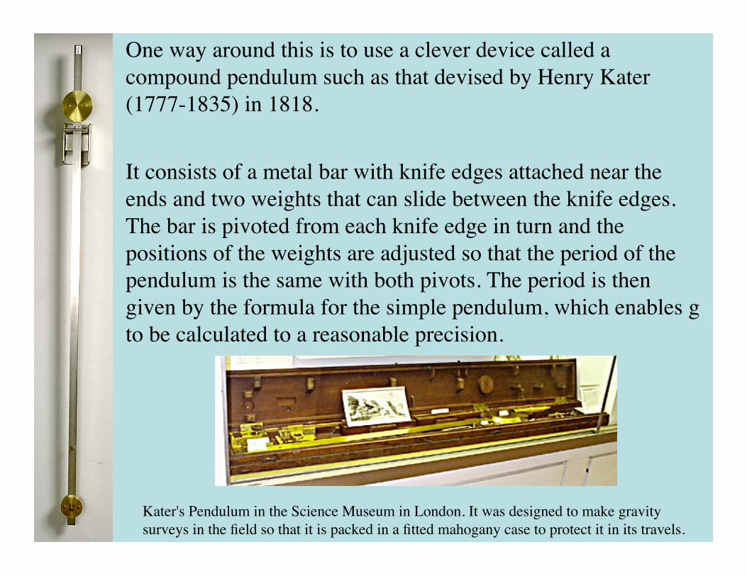
One way around this is to use a clever device called acompound pendulum such as that devised by Henry Kater(1777-1835) in 1818.

It consists of a metal bar with knife edges attached near theends and two weights that can slide between the knife edges.The bar is pivoted from each knife edge in turn and thepositions of the weights are adjusted so that the period of thependulum is the same with both pivots. The period is thengiven by the formula for the simple pendulum, which enables gto be calculated to a reasonable precision.

Kater's Pendulum in the Science Museum in London. It was designed to make gravitysurveys in the field so that it is packed in a fitted mahogany case to protect it in its travels.

Pendulums are not used much anymore but wereinstrumental (so to speak) in some of the major oildiscoveries of the early 20th century (Saudi Arabia,for example).

This is how Cecil Green got started.

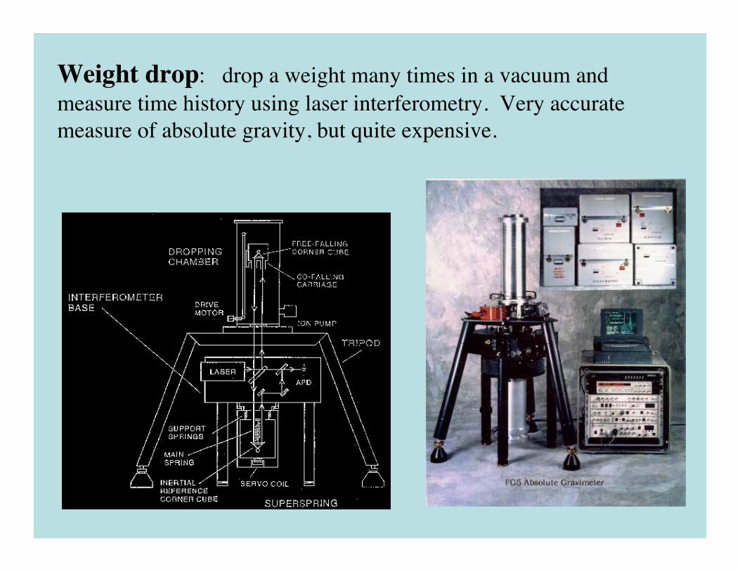
Weight drop: drop a weight many times in a vacuum andmeasure time history using laser interferometry. Very accuratemeasure of absolute gravity, but quite expensive.

Relative Measurements using a Mass on a Spring

At first glance this seems simple. We just use Hooke’s law:

F = mg = -kz

g = -(k/m)z

So that a change in g creates a change in z:

δg = -(k/m)δz

But the problem is sensitivity! δg/g = 10-8 = δz/z

So we need to have a really good way to measure the massdisplacement.

which is very long for a sensitive device! You wouldhave to wait forever to make a reading.

Nevertheless, remember that a very sensitive deviceshould have a very long period.

!

T = 2" mk

We could increase sensitivity by making k/m small, butthis would mean a combination of a big mass and aweak spring. Not good for field work!Additionally the system will oscillate with a period

A clever way around this problem wasdiscovered in 1934 by Lucien Lacoste, whowas trying to design a stable long periodseismometer.

He used a combination of geometry and adevice called a “zero-length spring”

Here’s how it works:

In the suspension suspension shown above, there are two torques:gravitational and spring.

If these two torques balance each other for any angle of the beam, thesystem will have infinite period. In this case, the smallest change invertical acceleration (or gravity) will cause a large movement.

Let’s see what’s required to meet this condition.

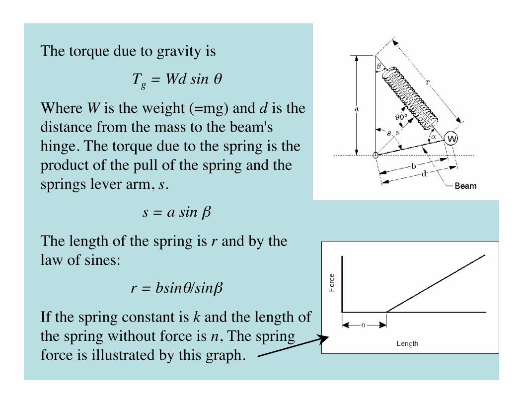
The torque due to gravity is

Tg = Wd sin θ

Where W is the weight (=mg) and d is thedistance from the mass to the beam'shinge. The torque due to the spring is theproduct of the pull of the spring and thesprings lever arm, s.

s = a sin β

The length of the spring is r and by thelaw of sines:

r = bsinθ/sinβ

If the spring constant is k and the length ofthe spring without force is n, The springforce is illustrated by this graph.

The torque due to the spring is then:

Ts = -k(r-n)s = kns -k(bsinθ/sinβ) a sin β = kns - kabsinθ

The total torque is then

To = Tg + Ts = Wdsinθ + kns - kabsinθ = kns + (Wd - kab)sinθ

This equation yields zero torque for allangles θ if:(1) n = 0 and(2) Wd - kab = 0The second part is easy and just involvesgeometry. For n to equal zero, we must havea "zero length spring". That is, a spring whoseforce-length graph passes through the origin or, at least, points towardthe origin. The turns of a helical spring of zero unstressed length wouldbump into each other before the spring actually reached zero length. Bymaking a helical spring whose turns press against each other when thereis no force on the spring, a "zero length spring" can be made.

There are several ways to make a zero length spring. A simplezero-length spring is a flat spiral spring. The mechanical propertiesof a spiral spring are not as convenient as a helical spring. Tomake a zero-length helical spring, the spring wire can be woundonto a mandrel. As the wire is wound, it can be twisted.

Another method is to hold the wire at an angle and with tensionwhile winding it on a rotating mandrel.

A problem that still needs to be faced is the sensitivity of the spring“constant” k to changes in pressure and temperature.

Pressure can be managed by evacuating the box.

Temperature effects are minimized with by keeping the box heatedto a temperature greater than any you are likely to encounter in thefield (50o C).

This last part means that the gravity meter consumes power - oftennot a convenient situation.

Nevertheless, the meter is very accurate and the drift rate is quitesmall, or in any event is linear and can be corrected for easily.

Views of theLacoste-Romberg

Gravity Meter

An second option is the Worden meter, which relies totally ongeometry to increase sensitivity, has an evacuated chamber, and usesdifferentially expanding materials to deal with temperaturevariations. It works ok, but the drift must be monitored closelywhen using it in the field.

Gravity measurements can be made at sea or in the air if you put it on agyroscopically controlled inertial table that corrects for the accelerationsof the boat or plane.

Reductions of Gravity DataGravity Measurements are not difficult to make, but the flip side is that

once you’ve made your measurements you need to do a fair amountof work before you can interpret them.

Here is an outline of the corrections you need to make to a rawmeasurement:

1. Latitude: Correction for N-S distance

2. Free-Air: Correction for elevation above the data plane

3. Bouguer: Correction for excess mass above the data plane

4. Terrain: Correction for variations in topography

5. Tides: Attraction of Sun and Moon

6. Eötvös: Correction for moving vehicle

7. Isostacy: Variations in crustal thickness

Latitude CorrectionThis is nothing more than accounting for the reference spheroid aspredicted by the International Gravity Formula.Recall that this formula (or variants on it) looks like:

g = 978.0318(1 + 0.005302sin2φg - 0.0000059sin22φg) cm/sec2

Note thatδg/δφ = 978.0318(0.0106048sinφgcosφg - 0.000235sin2φgcos2φg)

At 45o degrees latitude, δg/δφ = 5 gals/radian, or, because 1 radian= 57o degrees and 1o degree = 111 km:

δg/δφ = 0.8 mgal/km = 1.3 mgal/mile

Typically, we just calculate the reference gravity and subtract iffrom our readings, but this relation can be convenient.

Remember that gravity increases as you go towards the poles, sowe add this correction to our readings as we move to the equator.

Free-Air CorrectionOften we make observations at different elevations, and we know thatgravity will decrease as we get farther from the center of mass of theEarth.

Therefore, we choose a reference elevation (typically sea level) andadjust our readings to be what they would be at that elevation. Tocompute this correction, recall that

g = GM/r2

And so

δg/δr = -2GM/r3 = -2g/r = -0.3085 mgals/m = -0.09406 mgals/ft.

Most land surveys are done above sea level, so the free air correctionwill generally increase the gravity reading.

Bouguer CorrectionOf course, now that you have taken your reading down to sea level, youhave to account for all the mass between your original elevation and sealevel.This correction is called the “Bouguer Correction” (after our friendPierre) and is calculated by assuming an infinite slab of material ofthickness Δh lies between the station and sea level. We derived theexpression for this before:

Δgslab = 2πGΔρΔh

Assuming a typical density for crustal rocks (ρ = 2.67 gr/cm3), we arriveat

Δg = 0.112 mgals/m = 0.0341 mgals/ft

Again, because land surveys are usually above sea level, the Bouguercorrection usually decreases the gravity reading.

Terrain Corrections

Unless you do your survey in Kansas,you have to correct for variations intopography that you missed with yourinfinite slab. This is called a terraincorrection.Terrain corrections traditionally aremade by estimating the differencesbetween the elevation of the station andthat of the topography surrounding thestation.Remember that terrain always reducesthe gravity reading: mass excess abovethe station (mountains) pull up on thestation, while mass deficiencies below(valleys) “push” (the correction is for anegative mass).

Thus, a terrain corrected readingwill always be greater than itoriginally was.

Terrain correctionstraditionally were madewith something called a“Hammer” chart -namedafter the guy whointroduced them, andthey are truly the lowpoint of gravity work.

Hammer Charts

These charts divide the regions around the station into pie shapedcylindrical sections.The analyst centers the chart on the station location on a topo map andestimates the average elevation difference (note that this is in an absolutevalue sense!) for all elevations within the section.You multiply this number by a theoretical value for that section, and thenadd them all up.

Fortunately, we don’t have to do that much workanymore, because Digital Elevation Maps (DEMs)exist for much of the world, and for the US they arequite detailed (spacing of 10 m over much of thecountry).

Hence, most of this correction can be calculated bysuitable software; you only need to worry about anyterrain very close to the station (for example, if youhappen to be right by a cliff).

Aren’t you lucky?

TidesThe Sun and Moon can contribute 0.2-0.3 mgals of attraction and so weneed to correct for this if we are in the field for more than an hour or so(depends on desired accuracy, of course).

Some people advocatereoccupying a base stationseveral times to determinethis correction, but in factwe know how to calculateit better than most of uscan measure!

You should use thetheoretical correction.

EötvösIf you are making measurements in a moving vehicle, you have tocorrect for E-W velocity. As we discussed before, the verticalacceleration of a Eastward moving vehicle is:

Δac= 2ωvEcos(λ)

The effect is to decrease the reading taken from an eastward movingvehicle, and increase the reading from a westward moving one.

Isostatic correctionGravity studies can be useful in constraining crustal thickness, but oftenwe are not interested in structures that we can predict theoretically, so inmountainous terrain we oftenmake a correction for isostaticchanges in crustal thicknessdue to elevation.There are a number of waysto do this, from a pure Prattto pure Airy type ofcorrection.

Note that there is a strongrelation between theIsostatic anomaly and theFree Air anomaly.

Why should this be?

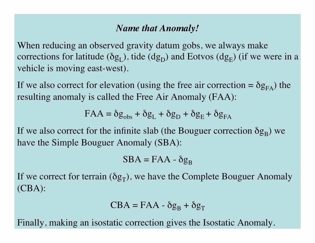
Name that Anomaly!

When reducing an observed gravity datum gobs, we always makecorrections for latitude (δgL), tide (dgD) and Eotvos (dgE) (if we were in avehicle is moving east-west).

If we also correct for elevation (using the free air correction = δgFA) theresulting anomaly is called the Free Air Anomaly (FAA):

FAA = δgobs + δgL + δgD + δgE + δgFA

If we also correct for the infinite slab (the Bouguer correction δgB) wehave the Simple Bouguer Anomaly (SBA):

SBA = FAA - δgB

If we correct for terrain (δgT), we have the Complete Bouguer Anomaly(CBA):

CBA = FAA - δgB + δgT

Finally, making an isostatic correction gives the Isostatic Anomaly.

Removing the Regional FieldThe Isostatic correction brings up a common problem: what to do whenwhat you are looking for is hidden in a big signal from some massanomaly far from you? Crustal thickness changes are a classicexample.

This “background” field is usually called the Regional Field because itis a long wavelength background that is typical of an entire “region”.There are some strategies for dealing with regionals, but be aware thatnothing is foolproof.

Most of these strategies involve removing a smooth background byfiltering or polynomial fitting.

Simple Example

More involved example (two-dimensional)

Example using Polynomials: Which is the Signal?

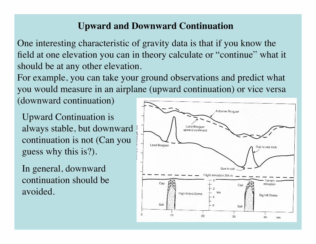
Upward and Downward Continuation

One interesting characteristic of gravity data is that if you know thefield at one elevation you can in theory calculate or “continue” what itshould be at any other elevation.For example, you can take your ground observations and predict whatyou would measure in an airplane (upward continuation) or vice versa(downward continuation)

Upward Continuation isalways stable, but downwardcontinuation is not (Can youguess why this is?).

In general, downwardcontinuation should beavoided.

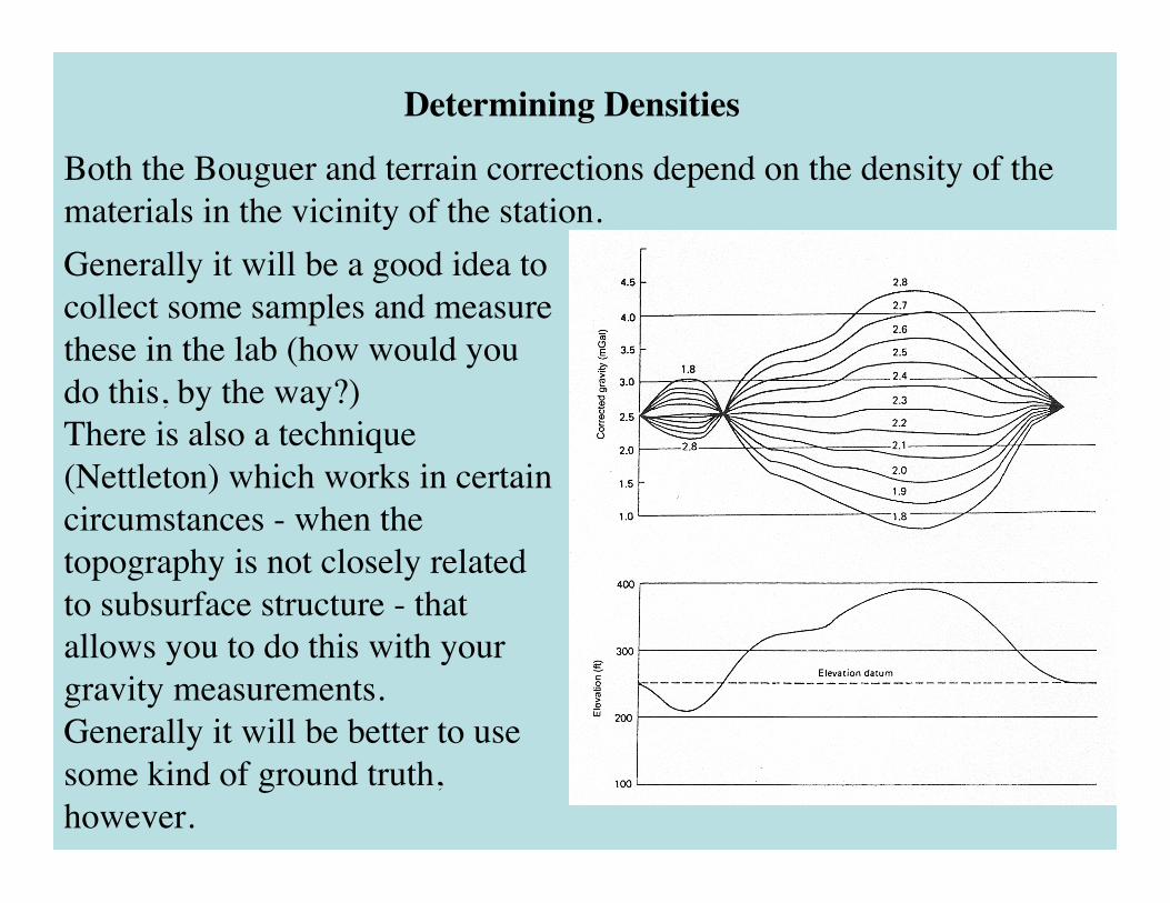
Generally it will be a good idea tocollect some samples and measurethese in the lab (how would youdo this, by the way?)There is also a technique(Nettleton) which works in certaincircumstances - when thetopography is not closely relatedto subsurface structure - thatallows you to do this with yourgravity measurements.Generally it will be better to usesome kind of ground truth,however.

Determining Densities

Both the Bouguer and terrain corrections depend on the density of thematerials in the vicinity of the station.

Examples of typical densityvariations are shown to theright.

Note that variations indensity are not much morethan a factor of 2 for mostrocks you are likely toencounter.