Measurement and Analytical Study of the Correlation ...cai/tvt-2014-measure.pdfIEEE TRANSACTIONS ON...

IEEE TRANSACTIONS ON VEHICULAR TECHNOLOGY, VOL. 63, NO. 9, NOVEMBER 2014 4165

Measurement and Analytical Study of theCorrelation Properties of Subchannel Fading for

Noncontiguous Carrier AggregationRuonan Zhang, Member, IEEE, Zhimeng Zhong, Yang Zhang, Stan Lu, and Lin Cai, Senior Member, IEEE

Abstract—The new multichannel/multicarrier technologies canpotentially support much higher data rates in mobile multiple-access environments, such as carrier aggregation (CA) defined inthe fourth-generation Long-Term Evolution Advanced enhance-ment. The correlation properties of noncontiguous subchannelsare critical for the performance of CA, including cell coverage,frequency diversity, and channel state estimation. This paperhas studied the correlation of the large-scale fading (LSF) andsmall-scale fading (SSF) of arbitrarily separated subchannels byrealistic channel measurement and analytical modeling. We firstobtain the subchannel correlation from the ultrawideband (UWB)channel measurement. This new approach avoids probing multiplesubchannels simultaneously with channel sounders, which wouldbe prohibitively complicated. The cross correlation of two distinctsubchannels and the autocorrelation of a single subchannel areevaluated. Second, a new propagation model for the Nakagami-mfading in a multipath environment is proposed. The frequency-domain level crossing rate (FD-LCR) is defined and derivedbased on the propagation model. Then, a Markov chain for thefrequency fading of the wideband channel is established, whichcan generate the correlated gain/power of subchannels in a widebandwidth. Therefore, this model can be used as a fast simulatorof CA over correlated subchannels. Finally, the cross correlationcoefficients (CCCs) between two Nakagami-m fading subchannelsobtained from the measurement and the proposed Markov modelare compared with the analytical results in the literature. Thispaper provides important insights into the fading correlation ofthe multicarrier channels and can be applied to the design andsimulation of indoor/outdoor multicarrier communications.

Index Terms—Carrier aggregation (CA), channel measurement,channel modeling, CLEAN, fading, ultrawideband (UWB).

Manuscript received February 8, 2013; revised July 5, 2013, October 21,2013, and January 14, 2014; accepted February 25, 2014. Date of publica-tion March 26, 2014; date of current version November 6, 2014. This workwas supported in part by the National Natural Science Foundation of Chinaunder Grant 61202394 and Grant 61301092, by the Ministry of Education ofChina through the Program for New Century Excellent Talents in Universityof China, by Northwestern Polytechnic University (NPU) through the NPUFundamental Research Program, by the Higher Education Doctoral ProgramFoundation under Grant 20116102120030, and by the Foundation for SelectedChinese Oversea Scholars. This paper was presented in part at the IEEE GlobalCommunications Conference, Anaheim, CA, USA, December 3–7, 2012. Thereview of this paper was coordinated by Prof. D. B. da Costa.

R. Zhang is with the School of Electronics and Information, NorthwesternPolytechnical University, Xi’an 710072, China (e-mail: [email protected]).

Z. Zhong and S. Lu are with Huawei Technologies Ltd., Xi’an 710065, China(e-mail: [email protected]; [email protected]).

Y. Zhang is with Xidian University, Xi’an 710126, China.L. Cai is with the Department of Electrical and Computer Engineering, Uni-

versity of Victoria, Victoria, BC V8W 2Y2, Canada (e-mail: [email protected]).Color versions of one or more of the figures in this paper are available online

at http://ieeexplore.ieee.org.Digital Object Identifier 10.1109/TVT.2014.2314028

I. INTRODUCTION

MULTICHANNEL/MULTICARRIER technologies haverecently attracted increasing interest due to their higher

data rate capacity and flexibility in spectrum allocation andmultiple access. For example, carrier aggregation (CA) hasbeen proposed as an enhancement to Long Term Evolution(LTE) Advanced [1] where a terminal may combine severalsubchannels (e.g., with the bandwidth of 20 MHz). Becauseaggregating noncontiguous available subchannels is supported,CA may further exploit the frequency diversity.

Since the existence of multipath propagation gives rise tofrequency-selective fading channels, the correlation betweenthe aggregated subchannels in CA plays an important role inthe performance of the multicarrier transmission. One of thepotential applications of the correlation of the large-scale fading(LSF) of the subchannels is analysis of the cell coverage. Weknow that the capacity of one subchannel between a base station(BS) and a mobile station (MS) depends on the received SNRaccording to the Shannon theory, and the SNR is determinedby the LSF (i.e., the path loss (PL) and shadowing). Now,the problem is if there is a significant difference between theaverage capacities of two separated subchannels or if is itpossible to get much higher capacity when we switch fromone subchannel to another. Another application is channel stateestimation. The channel gain is usually estimated to performautomatic gain control at the receiver and automatic modulationand coding at the transmitter [2]. In CA, how much are thetwo subchannels separated such that their states are similar?Given the similarity of subchannel states, estimation of onesubchannel may be sufficient, and the other estimation cost canbe reduced. Furthermore, the frequency diversity gain achievedby CA also depends on the subchannel correlation. The answersto both questions depend on the correlation of the small-scalefading (SSF) between the two subchannels.

Therefore, it is important to quantify the correlation of thetwo subchannels that may be arbitrarily separated. In [3],Filho et al. derived the accurate closed-form expression forthe cross correlation function (CCF) between two noniden-tically distributed Nakagami-m fading processes with time,space, and/or frequency spacing. Thus, the cross correlationcoefficient (CCC) can be obtained analytically. This insightfulwork provides a very useful theoretical study on the correlationproperty needed for CA. However, to the best of our knowl-edge, realistic measurements on the correlation, with respectto frequency spacing, have not been reported in the literature.

0018-9545 © 2014 IEEE. Personal use is permitted, but republication/redistribution requires IEEE permission.See http://www.ieee.org/publications_standards/publications/rights/index.html for more information.

4166 IEEE TRANSACTIONS ON VEHICULAR TECHNOLOGY, VOL. 63, NO. 9, NOVEMBER 2014

The key reason is that, using the traditional channel soundingtechnology, the sounder needs to simultaneously probe multi-ple subchannels, which requires prohibitively high complexity.As specified in [4], the initial identified bands for CA arenonuniformly scattered from 0.4 to 5 GHz. Elektrobit andMedav are two companies with sound reputations in channelmeasurement around the world. However, their state-of-the-artchannel sounders, named Propsound and RUSK, respectively,cannot support simultaneous multiband probing across giga-hertz spacing. This motivated us to search for an alternativeapproach to tackling this problem.

Furthermore, it is useful to design a multisubchannel sim-ulator that can directly generate the correlated Nakagami-mfading subchannel states fast and easily. The finite-state Markovchain (FSMC) model, which can generate the correlated time-varying fading channel states, has been proposed and widelyused in the simulation and analytical study of the traditionalmobile communication systems and upper layer packet-basedprotocols [5]. Is it possible to establish an FSMC to generatethe correlated subchannel states in the frequency domain?

In this paper, the correlation of the LSF and SSF of thesubchannels is investigated from two aspects: the realistic mea-surement and the Markovian modeling. We consider a generalmulticarrier system as follows. The operator is licensed with awideband spectrum over a couple of gigahertz, called the oper-ator channel. The operator channel is divided into a number ofsubchannels (i.e., subbands) of several kilohertz or megahertz,which are assigned to different users and can be aggregated byCA. The subchannels have approximately flat fading. Our targetis to quantify the correlation of the LSF and the SSF of thesubchannels. The LSF refers to the shadowing effect caused byobstructors, which, for the indoor scenario, typically happenswhen the receiver moves from one room to another. The SSFrefers to the frequency-selective fading caused by the multipathpropagation.

The main contributions of this paper are twofold. First, wedevelop an alternative approach based on the indoor ultraw-ideband (UWB) channel measurement. The idea is to extractthe fading information of various subchannels from the UWBchannel frequency response, which is obtained by probing thechannel with nanosecond-level pulses. This technique not onlyavoids the traditional complicated sounder implementation butis also convenient for extracting the subchannel power densitywith various central frequencies and bandwidths. A compre-hensive study is presented, including: 1) the cross correlationof the LSF and of the SSF of two separated subchannels, and2) the autocorrelation of the LSF and the SSF of one singlesubchannel.

Second, a frequency-domain FSMC (FD-FSMC) model de-scribing the power spectrum density (PSD) is proposed, whichcan generate the correlated states of the subchannels sequen-tially. We propose a propagation model for the subchannelNakagami-m fading process. Then, the frequency-domain levelcrossing rate (FD-LCR) for a wideband frequency-selectivechannel is defined and derived, based on which the transitionprobabilities of the FD-FSMC is determined. Finally, the CCCof two subchannels obtained from the measurement and the FD-FSMC are compared with the analytical result in [3].

The remainder of this paper is structured as follows. Webriefly provide an overview the related work and the UWBchannel measurement in Section II. The modified CLEANalgorithm and the process of obtaining the LSF and the SSFof the subchannels are proposed in Sections III and IV, respec-tively. The correlation of the spatial fading of the subchannelsare evaluated in Section V based on the measurement results.The propagation model and FD-LCR of the subchannels areproposed in Section VI. Section VII presents the FSMC toevaluate the SSF correlation analytically. The analytical andmeasurement results are compared in Section VIII to validatethe channel model. Section IX concludes this paper and indi-cates further research issues.

II. RELATED WORK AND ULTRAWIDEBAND

PROPAGATION MEASUREMENT

A. Correlation of Two Channels With Frequency Separation

While extensive research has been carried out for the physicalLTE channel measurement and modeling [6], only a handfulof papers has considered the correlation between subchannels.In [7] and [8], and [9], the LSF correlation for outdoor andindoor scenarios, respectively, has been studied. Due to the limitof the channel sounders, only the correlation between severalwireless links with fixed frequencies were measured. The an-alytical results of the CCF between nonidentical Nakagami-mfading processes with space, time, and frequency spacing werepresented in [3] and [10]. The closed-form expression for CCCis [3, eq. (1)]

R(τ, Δω) =

(Ω1

m1

) 12(Ω2

m2

) 12

[Γ(m1 +

12

)Γ(m2 +

12

)Γ(m1)Γ(m2)

]

× 2F1

(−1

2, −1

2; m2; ρ

)

≈√

m1

m2ρ(τ, Δω) (1)

where Ω1 and Ω2 are the average power values of theNakagami-m fading processes, Γ(·) is the gamma function,and 2F1(·, ·; ·; ·) is the hypergeometric function. In (1), ρ is theautocorrelation coefficient of the underlying Gaussian randomcomponents [11]. To consider two fading instances with thetime and frequency separation of τ and Δω (in radians persecond) received on one omnidirectional antenna, we have[3, eq. (5)]

ρ(τ, Δω) =J20 (ωDτ)

1 + (ΔωT )2(2)

where ωD = 2πfD is the maximum Doppler shift in radiansper second, J2

0 (·) is the Bessel function of the first kind andzeroth order, and T is the mean excess delay of the scatteredwaves. The analytical works in [3] and [11] are very insightfulas they derived the unified closed-form expression for thegeneric-order CCF of two Nakagami-m fading instances witharbitrary temporal, frequency, and spatial separation. However,the practical measurement of the subchannel correlation withfrequency separation is still rarely reported in the literature.

ZHANG et al.: CORRELATION PROPERTIES OF SUBCHANNEL FADING FOR NONCONTIGUOUS CA 4167

On the other hand, to conduct analysis and simulation ofcommunication systems and upper layer protocols taking intoaccount the correlated variation of wireless channels, a simplestochastic channel model is very useful. The FSMC modelhas been proposed to describe the temporal variation of singleor even diversity-combined Rayleigh and Nakagami-m fadingprocesses [5], [12]. Because these models can generate thecorrelated channel states for discrete time instances (e.g., everypacket transmission interval) and can be also easily incorpo-rated into the packet-level analysis frameworks of upper layerprotocols, they have been widely used in the simulation andanalysis of traditional narrow-band systems. The time-domainFSMCs are established based on the higher order statistics,i.e., LCR, of the fading channel. Establishing the FSMC modelfor the frequency-selective fading between subchannels withappropriate correlation motivates the work in this paper.

Following the previous approach, it is critical to determinethe FD-LCR between the gain/power of subchannels. In theearly work of [13], the LCR of the channel’s transfer functionwas investigated from the Fourier transform of the powerdelay profile (PDP) model for the frequency-selective Ricianfading channel. In [14], the channel gain LCR between adja-cent subchannels in orthogonal frequency-division multiplex-ing (OFDM) systems was obtained based on the Jakes’ model.In [15], a novel general framework to calculate the LCR andthe average fade duration (AFD) of a sampled fading channelwas presented. The authors applied the method to the frequencyresponse envelope in an OFDM system. In this paper, we extendthe work in [14] for a general wideband radio channel. Fur-thermore, the CCC between two subchannels in the developedFSMC is compared with both the measurement and analyticalresults [3], [10]. The objective of this paper is to provide a fastsimulator to support the wideband channel modeling and designof multicarrier communications such as CA.

B. UWB Channel Measurement

The characterization of the subchannel correlation in this pa-per is based on the UWB propagation measurement performedin a typical modern office building [16]. The measurementis briefly reviewed for convenience. The placement of thetransmitter and 14 receiving regions are shown on the floor planin Fig. 1(a). In each region, the receiver antenna was placedat 49 positions arranged spatially on a 7 × 7 square grid with15-cm spacing, as shown in Fig. 1(b). The point on the ith rowand jth column on the grid is indexed as (i, j). As a convention,the first row is always parallel and adjacent to the north wall ofthe room.

The two diamond-dipole UWB antennas are vertically polar-ized and nearly circularly symmetric about their vertical axes[18]. The pulser at the transmitter generates Gaussian-shapedpulses with 2-ns duration periodically to probe the channel. Theresponse waveform is recorded by a digital sampling oscillo-scope for a 300-ns time window. Since the antennas and otherprocessing apparatus may differentiate and filter the pulser’soutput due to their implicit bandlimiting and frequency-selective effect, the received pulses may be severely distorted.Fig. 2(a) shows the three reference waveforms recorded with1-m transceiver separation and the receive antenna rotated by

Fig. 1. Floor plan of the office building and the measurement grid [17].(a) Building floor plan. (b) Measurement grid.

Fig. 2. Received clean pulses at 1-m separation distance and pulse template.(a) Measured in three angles. (b) Averaged and power normalized.

0◦, 45◦, and 90◦, respectively. According to the environment,the earliest multipath component (MPC) reflected from scatter-ers arrives about 4 ns after the line-of-sight (LOS) signal. Thus,Fig. 2(a) represents the clean pulses propagated via the LOSpath without being corrupted by the MPCs, which embody thecharacteristics of the pulse driver and the antenna systems.

Substantial variation in the SNR of the recorded waveformsat different locations is observed. The SNR in the offices closeto the edge of the building is much lower, due to large PL andexternal radio inferences. Therefore, the measurement results inrooms B and C are excluded from the following analysis.

III. CLEAN ALGORITHM AND CHANNEL IMPULSE

RESPONSE EXTRACTION

The approach to identifying the fading of subchannels fromthe UWB propagation measurements includes three steps. Wefirst extract the UWB CIRs from each individual measurement,using a modified CLEAN algorithm [19]. Then, the frequencyresponse and the PSD are obtained by performing Fouriertransform of the channel impulse responses (CIRs). Finally, thepower of subbands is acquired by integrating the PSD over thecorresponding bandwidth.


A. Modified CLEAN Algorithm

The impulse response of the multipath channels is often mod-eled as the summation of discernible paths with different timedelays, amplitude attenuation, and phase shift, expressed by

h(t) =

N∑n

anδ(t− τn) (3)

where an and τn are the complex magnitude and delay of thenth propagation path, respectively. When probing the channelwith short pulses, as previously mentioned, the receivedwaveform is a bandlimited and distorted form of the pulsesdriving the transmitter’s antenna, which is denoted p(t). Atypical multipath model for the observed response, which isdenoted r(t), is

r(t) =

N∑n

anp(t− τn). (4)

If p(t) is known, deconvolution techniques can resolve an andτn such that a continuous-time CIR, which is denoted h(t), canbe extracted from the measured waveform.

A simple deconvolution technique involves the inverse filter-ing. The channel transfer function can be estimated by H(ω) =R(ω)/P (ω), where R(ω) and P (ω) are the Fourier transformsof r(t) and p(t), respectively. However, this approach is sus-ceptible to high noise levels, which may generate several near-coincidental and opposing taps from a single impulse plus noise[20]. Another technique is the CLEAN algorithm, which isinitially used to enhance radio-astronomical images [21] andhas been applied to UWB channel characterization [20], [22].The CLEAN algorithm performs subtractive deconvolution,identifying impulses directly from the waveform; therefore, thisapproach is less prone to noise. However, different from theoriginal CLEAN algorithm for astronomical image processing,we need to decide the propagation paths for CIR extraction.Setting the threshold for recognizing paths is nontrivial. Thisis mainly because, in the practical measurement, the distancebetween the transceivers changes significantly, resulting in thelarge variation of the power of the captured signal. If thethreshold is too low, many pseudopaths may be identified,whereas if it is too high, some true paths can be missed. SinceWin’s set of measurement data shows substantial variation inthe noise power, adopting a fixed threshold may not be suitable.Motivated by this fact, we propose adjusting the threshold foreach measurement snapshot adaptively according to the noiselevel.

We take the average of the three clean pulses in Fig. 2(a) anduse the waveform from 4.73 to 7.56 ns as the final clean pulse,as plotted in Fig. 2(b) (the x-axes have been reset to start from0). The clean pulse is denoted p(t). Furthermore, to obtain theamplitude (or energy) of the impulses in the CIR, the energy ofp(t) is normalized by

p(t) =p(t)∫ T

o p2(t)dt(5)

where T is the pulse duration. p(t) is used as the template pulsein the deconvolution.

The proposed deconvolution approach is performed by thesteps in Algorithm 1.

Algorithm 1 Iteration Steps of modified CLEAN Algorithm

Require: r(t): captured waveform, p(t): pulse template, Tw:duration of r(t), Tn: duration of the noise waveform;

Ensure: h(t): estimated CIR;1: n(t) = r(t+ Tw − Tn), t ∈ [0, Tn];2: Υ(τ) =

∫ τ+T

τ n(t)p(t− τ)dt;3: Set γ0 such that cdfΥ(γ0) = 90%;4: d(t) = r(t), t ∈ [0, Tw − Tn];5: c(t) = 0 and Φ = { };6: Γ(τ) =

∫ τ+T

τ d(t)p(t− τ)dt;7: τM = argmaxτ{|Γ(τ)|} and γM = Γ(τM );8: while γM >= γ0 and τM ! ∈ Φ do9: Φ = Φ ∪ {τM};10: c(t) = c(t) + γMδ(t− τM );11: d(t) = d(t)− γM p(t− τM );12: Γ(τ) =

∫ τ+T

τ d(t)p(t− τ)dt;13: τM = argmaxτ{|Γ(τ)|} and γM = Γ(τM );14: end while15: h(t) = c(t) =

∑γ(i)M δ(t− τ

(i)M )

The first three steps determine an appropriate power thresh-old, which is used to distinguish if the correlation is p(t)with a received pulse through a propagation path or with thebackground noise in the following steps. By observing thecaptured channel responses with the duration of Tw = 299.8 nsin all the measurements, the excess delay is no more than250 ns. Thus, the last 50-ns waveform is just background noiseand is used to estimate the range of the correlation coefficient ofp(t) with noise. Therefore, step 1 extracts the last Tn = 50 nswaveform from the captured signal as the noise. By calculatingthe correlation coefficient function, step 2 gives a sample setof the correlation results of the template pulse p(t) and thebackground noise for a certain measurement point. Step 3 setsthe decision threshold as γ0, which is the 90th percentile of thedistribution of Υ(τ). Consequently, if the correlation coefficientof a waveform and p(t) is smaller than γ0, the waveform isquite likely just background noise. Otherwise, we regard thatthe waveform contains a copy of the signal and then extract thegain of the path in the following steps.

Step 4 sets the dirty map by the captured waveform withthe noise sequence of n(t) removed. Step 5 initializes theclean map c(t) and the path delay set Φ, respectively. Step 6forms the correlation function of the dirty map d(t) and thetemplate p(t), which would peak at the delays of the MPCs.Then, we obtain the delay and the corresponding polarizedpower of the maximal amplitude of Γ(τ) by step 7, where | · |takes the absolute value. Steps 9–13 perform the iteration ofthe CLEAN algorithm to extract the path information. Once apath is identified by checking the correlation function, the setΦ and the clean map ct are updated by adding the delay andthe corresponding impulse in steps 9 and 10, respectively. Thedirty map is then cleaned by subtracting the scaled and delayed


Fig. 3. Received waveforms and extracted CIRs. (a) Received waveform.(b) CIR.

template pulse in step 11. Steps 12 and 13 are the same assteps 6 and 7 but are performed iteratively inside the loop. Ifthe stopping criteria in the WHILE statement is not satisfied,i.e., even the correlation function peak is produced by thecorrelation with noise or has already occurred in the previousiterations, the iteration finishes, and the estimated valid pathshave all been identified.

Finally, the CIR extracted from r(t) is organized in step 15,where γ

(i)M and τ

(i)M are the recorded correlation function peaks

and the corresponding delays in the iterations. In summary, thealgorithm above is designed to adapt to the substantially vary-ing noise floor and is simple to implement, which is suitable forprocessing the indoor UWB channel measurements.

B. Extracted CIRs of Typical Scenarios

The extracted CIRs of some typical scenarios using theCLEAN algorithm are demonstrated in Fig. 3, where the orig-inal waveforms are recorded at the center positions of threeregions. Regions F1, N , and A are representative for the LOS,non-LOS (NLOS) with high SNR, and NLOS with low SNRscenarios (longer propagation distance and more obstructors),respectively. It can be seen that the multipath profiles havean obvious cluster-arriving and double exponentially decayingpattern. Note that the signal magnitude for NLOS is attenuatedsignificantly.

The time resolution of the CLEAN algorithm is equal to thewidth of the main lobe of the autocorrelation function of thetemplate pulse. The narrower the autocorrelation function is,the higher the time resolution of the extracted CIR. Hence,the UWB probing pulse makes it possible to characterize thechannel frequency response within a high bandwidth.

Fig. 4. Power attenuation in 2–6 GHz of SSA-PSD versus logarithm distance.

IV. FINDING SUBCHANNEL FADING

In most of the existing channel models, the propagation lossis presented by the product of the PL, LSF, and SSF. Further-more, due to the frequency-dependent propagation effects, theloss is a function of frequency and of distance.

We are interested in the total bandwidth of 2–6 GHz, and thebandwidth of one subchannel is 20 MHz. The received powerof the subchannels and that of the frequency-dependent fadingare investigated based on the PSD, which is G(f) = |H(f)|2,where H(f) is the channel frequency response obtained by theFourier transform of h(t). Then, the received power of a sub-channel is acquired by integrating G(f) over the correspondingbandwidth [19].

A. Averaging SSF Within Measurement Regions

PL and SSF should be removed from the received power at-tenuation to estimate the LSF of the subchannels. As previouslymentioned, the SSF for this indoor UWB channel measurementis introduced when the receiver moves over the region gridwithin a room.

We refer to the PSD obtained at a grid point as the individualPSD, whereas the PSD averaged over the 49 positions withinone region is denoted as the SSF spatial-averaged PSD (SSA-PSD). The center frequency of our bandwidth of interest is4 GHz; therefore, the grid edge of 90-cm length is approx-imately of 10λ, which is proposed as a good window sizeto average out SSF without distorting the LSF patterns forindoor multipath propagation [9], [23]. Then, the LSF may beinvestigated by analyzing the variation of the SSA-PSDs overdifferent regions (i.e., rooms).

B. Extracting the PL Within Interested Bandwidth

By integrating the SSA-PSD over the 2–6 GHz bandwidth,we obtain the average total energy of each region, which isdenoted PX where X represents the alphabet of the region(e.g., X is F1, A, E, etc.). The total energy of the referencemeasurement (with a separation distance of d0 = 1 m) can beacquired in the same way, which is denoted P0. Then, the powerattenuation for region X can be defined as AX = P0/PX . Assuggested by the scatter plot in Fig. 4, we obtain the linearregression of the measured power attenuation (in decibels) as


a function of the logarithm of the transceiver distance. The PLmodel of the empirical attenuation is

PL(d)dB = 10 log10

(P0

¯P (d)

)= 32.02 log10

(d

d0

)− 7.75

(6)

where ¯P (d) is the expected received power averaged over boththe LSF and SSF at distance d.

C. Finding the Subchannel LSF and SSF

Because we are interested in the correlation of the subchan-nel LSF (i.e., the average power variation), for easy calculation,we approximate that all the subchannels have the same PLexponent. In other words, the slope of the linear PL model (indecibels) is the same within the total bandwidth of interest.This approximation does not affect the evaluation of LSFcorrelation because we are interested in the variation of thepower attenuation.

As previously mentioned, there are a total of 200 subchannelsinside the bandwidth of 2–6 GHz. Suppose that the receivedpower of the kth subchannel in the reference measurement isP

(k)0 . Thus, the expected received power for the subchannel at

a measurement region is¯

P(k)X = P

(k)0 /PL(dX), where PL(dX)

is obtained from (6). The SSF-averaged received power of thesubchannel is obtained by integrating the SSA-PSD over the

subchannel bandwidth, which is denoted¯

P(k)X . Then, the LSF

of the subchannel is Y (k)X =

¯P

(k)X − ¯

P(k)X .

The small-scale statistics are derived by considering thedeviations of the 49 local PSDs from the SSA-PSD. The re-ceived power of the kth subchannel at the measurement position(i, j), which is denoted P

(k)X, ij , is obtained by integrating the

local PSD over the bandwidth. Hence, the SSF is Z(k)X, ij =

¯P

(k)X − P

(k)X, ij .

V. CORRELATION OF THE SUBCHANNEL FADING

The study of the spatial variation of the subchannels includestwo aspects [19]: 1) the cross correlation of the LSF and SSFof two different subchannels, and 2) the autocorrelation of theLSF and the SSF of one single subchannel.

A. Cross Correlation of the LSF of Two Subchannels

The LSFs of the kth and lth subchannels are denoted bythe random variables (RVs) Y

(k)sub and Y

(l)sub, respectively. The

measured LSFs obtained from the SSA-PSDs of the ten NLOSregions are the samples of the two RVs (as previously men-tioned, regions B and C are excluded due to very high noisefloor). Then, the CCC can be calculated as follows:

ρk, l =cov

(Y

(k)sub , Y

(l)sub

)√

var(Y

(k)sub

)var

(Y

(l)sub

) (7)

where cov(·) and var(·) are the covariance and variance of thegiven RV(s), respectively.

Fig. 5. CCC of the LSF of two subchannels.

Fig. 6. CCC of the SSF of two subchannels.

Fig. 5(a) shows ρk, l when the bandwidth of both subchannelsis 20 MHz, the lower bound frequency of one subchannel isfixed at 2 GHz, and that of the other increases from 2 to3.98 GHz. Thus, the separation of them increases from 0 toalmost 2 GHz. Fig. 5(b) shows a similar case, but the lowerbound frequency of one subchannel is fixed at 4 GHz and thatof the other changes from 4 to 5.98 GHz. Furthermore, theautoregression of the measurement results averaged by a slidingwindow with the size of 20 is also plotted by the dashed lines,to remove the random fluctuation of the measurements.

As shown, the LSF of two subchannels is close to fullcorrelation, with the correlation coefficient mostly larger than0.9. This is not surprising because the shadowing effect causedby obstructors should be consistent for the subchannels insidethe bandwidth of interest. Furthermore, comparison of the twosubfigures also illustrate that the averaged correlation coeffi-cient is always about 0.95, independent from the frequencyseparation and the central frequencies.

B. Cross Correlation of the SSF of Two Subchannels

When the receiver moves over a measurement region grid,the SSF of a subchannel (i.e., the difference of the receivedpower obtained at a position and that of the SSA-PSD) is anRV. The SSF of the kth and lth subchannels are denoted bythe two RVs Z

(k)sub and Z

(l)sub, respectively. For a given region,

the measured SSF of the two subchannels at the grid pointsZ

(k)X, ij and Z

(l)X, ij can be regarded as the 49 observations of Z(k)

sub

and Z(l)sub, respectively. Then, the CCC is calculated similarly

according to (7).Fig. 6 shows ρk, l of two regions, F1 (LOS scenario) and E

(NLOS scenario), presented in the same way as in Fig. 5(b). It isobserved that the correlation reduces quickly with the increasein the separation of the two subchannels. The decorrelation


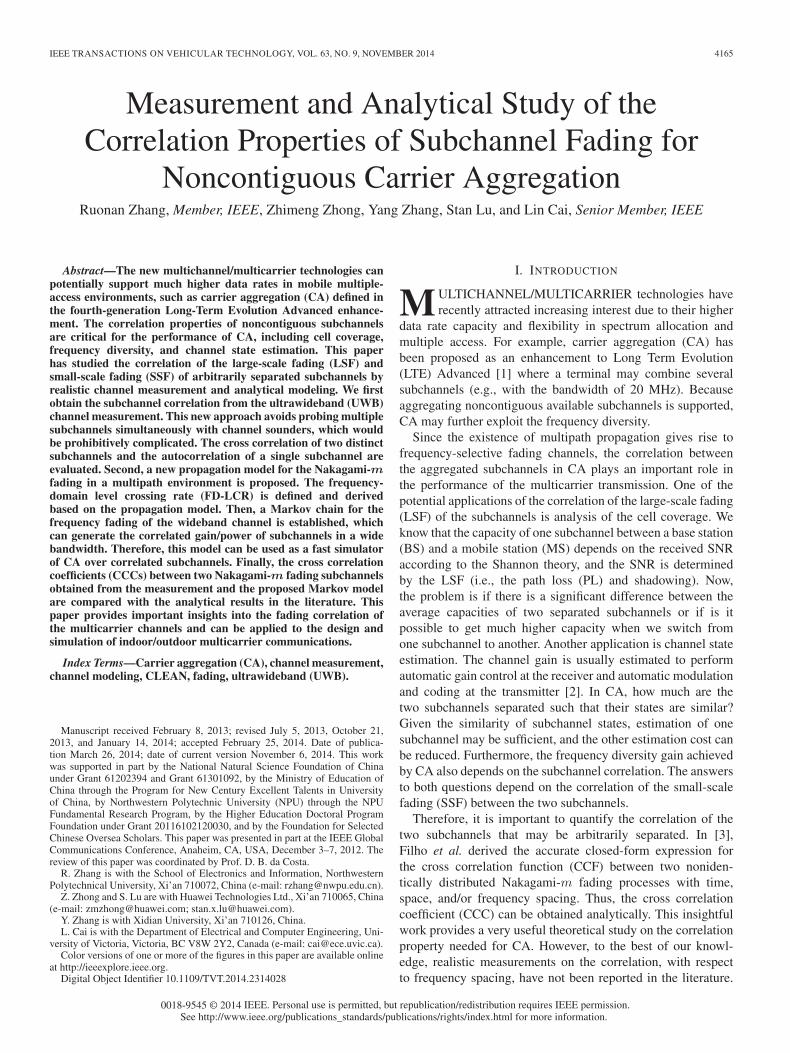
Fig. 7. Autocorrelation coefficient of the LSF of a single subchannel.

distance is less than 100 MHz, by which the coefficient hasdropped to below 0.2. One possible explanation is that theintensive multipath effect in an indoor environment results insevere superimposition of the MPCs at the receiver. With asmall change in the frequency, the in-phase enhancement andout-of-phase cancelation will vary dramatically. Thus, the SSFis quite sensitive to the carrier frequency. In addition, we can seethat the correlation coefficient of the LOS scenario is slightlylarger than that of the NLOS scenario. This is expected sincethe LOS component does not have the superimposition effectand hence remains consistent for frequency change.

C. Autocorrelation of the LSF of a Subchannel

The autocorrelation of the LSF refers to a single subchannelfor the NLOS scenario. The measured LSF of the kth subchan-nel Y (k)

X obtained from the SSA-PSD of the ten NLOS regionscan be regarded as a random sequence. The autocorrelation ofthe sequence can be calculated. The results of two representa-tive subchannels, i.e., 2–2.02 and 4–4.02 GHz, are shown inFig. 7. The x-axis is the index of the measurement regions,which are reordered such that the distance to the transmitteris increasing.

As shown, the LSF of a single subchannel is almost uncor-related for different rooms. This is expected because the shad-owing effect is mostly specific to the surrounding environment.Similar results were observed in [9], where the decorrelationdistance for the LSF of an indoor wireless link is on the orderof 1–2 m.

D. Autocorrelation of the SSF of a Subchannel

The autocorrelation of the SSF of one subchannel can betreated in the same way as earlier in the frequency domain.However, since the autocorrelation actually depends on thevariation of the CIR for the movement of the receiver withina small distance (such as several wavelengths), the variationof the PDP in the time domain reflects the variation of thepower of subchannels. Therefore, we choose to directly studythe autocorrelation of PDP here. In this way, we can also seehow the wideband CIR changes in the time domain.

The measured PDPs at all positions in a region are alignedand quantized. First, each local PDP is aligned by an appropri-ate delay reference, removing the background noise before thearrival of the true response signal in the recorded waveform. Asin [17], we take the reference delay as the absolute propagation

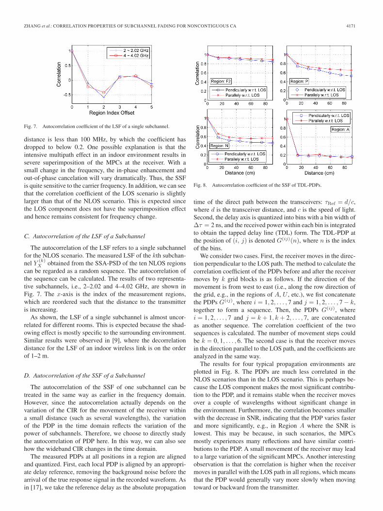
Fig. 8. Autocorrelation coefficient of the SSF of TDL-PDPs.

time of the direct path between the transceivers: τRef = d/c,where d is the transceiver distance, and c is the speed of light.Second, the delay axis is quantized into bins with a bin width ofΔτ = 2 ns, and the received power within each bin is integratedto obtain the tapped delay line (TDL) form. The TDL-PDP atthe position of (i, j) is denoted G(ij)(n), where n is the indexof the bins.

We consider two cases. First, the receiver moves in the direc-tion perpendicular to the LOS path. The method to calculate thecorrelation coefficient of the PDPs before and after the receivermoves by k grid blocks is as follows. If the direction of themovement is from west to east (i.e., along the row direction ofthe grid, e.g., in the regions of A, U , etc.), we fist concatenatethe PDPs G(ij), where i = 1, 2, . . . , 7 and j = 1, 2, . . . , 7 − k,together to form a sequence. Then, the PDPs G(ij), wherei = 1, 2, . . . , 7 and j = k + 1, k + 2, . . . , 7, are concatenatedas another sequence. The correlation coefficient of the twosequences is calculated. The number of movement steps couldbe k = 0, 1, . . . , 6. The second case is that the receiver movesin the direction parallel to the LOS path, and the coefficients areanalyzed in the same way.

The results for four typical propagation environments areplotted in Fig. 8. The PDPs are much less correlated in theNLOS scenarios than in the LOS scenario. This is perhaps be-cause the LOS component makes the most significant contribu-tion to the PDP, and it remains stable when the receiver movesover a couple of wavelengths without significant change inthe environment. Furthermore, the correlation becomes smallerwith the decrease in SNR, indicating that the PDP varies fasterand more significantly, e.g., in Region A where the SNR islowest. This may be because, in such scenarios, the MPCsmostly experiences many reflections and have similar contri-butions to the PDP. A small movement of the receiver may leadto a large variation of the significant MPCs. Another interestingobservation is that the correlation is higher when the receivermoves in parallel with the LOS path in all regions, which meansthat the PDP would generally vary more slowly when movingtoward or backward from the transmitter.


VI. FADING MODEL OF SUBCHANNELS

Inspired by the measurement results in Section V, we pro-pose an FSMC model to describe the correlation of the SSF oftwo separated subchannels here. We consider a static multipathpropagation channel, where there are a number of scatterersaround. Suppose that the PDP of the wideband operator channelhas exponentially decaying pattern, as shown in Fig. 3. Thenarrow-band subchannels is modeled by Nakagami-m fading,which is more general and suitable for indoor environmentsthan the Rayleigh distribution. The simulation results obtainedof the model will be compared with the measurement results inSection VIII.

A. Average PDP of Wideband Operator Channel

Typically, the exponentially decaying PDP can be express-ed as

P (τ) = A exp

(− τ

τRMS

)(8)

where τ is the excess delay, τRMS is the RMS delay spread,and A is the maximum received power at τ = 0 (i.e., the firstarrived MPC). Since the physical propagation environmentsare random, (8) can be regarded as the average PDP of themultipath channels.

We consider the valid MPCs whose received power (i.e.,the square of the channel gain) is above the threshold, whichis defined as αA, where α is the threshold coefficient (e.g.,α = 0.1). Therefore, the maximal excess delay of the validMPCs is

τM = −τRMS · lnα. (9)

B. Multipath Propagation Model of Subchannels

The bandwidth of a subchannel for one user is denoted Bs.The CIR of a narrow-band subchannel is the superposition ofthe MPCs, which results in the flat fading. Suppose there areN valid MPCs and the excess delay and power of the jth MPCare τj and P (τj), respectively. Without loss of generality, weassume that τj is uniformly distributed from 0 to τM , i.e., τj ∼U [0, τM ], where τM is defined as in (9). Thus, the receivedsignal of a subchannel, which is the superposition of the MPCs,can be expressed as{

x(fc) =∑N

j=1 aj cos (2πτjfc + θj)

y(fc) =∑N

j=1 aj sin (2πτjfc + θj)(10)

where fc is the carrier frequency of the subchannel, and x(fc)and y(fc) are the superposition of the in-phase and quadraturecomponents of the N paths, respectively. θj is the random phaseshift caused by the reflection and/or diffraction on the jth pathand is approximated by uniform distribution θj ∼ U [0, 2π). ajis the signal amplitude of the jth path, and its expectation is

E[aj ] =√

P (τj) =

√A exp

(− τjτRMS

). (11)

The number of paths N is usually large enough so that x(fc)and y(fc) can be considered being normally distributed due tothe central limit theorem. By derivation, we can get E[x(fc)] =E[y(fc)] = 0 and

E[x2(fc)

]= E

[y2(fc)

]=

12

N∑j=1

E[a2j]=

NA(α− 1)2 lnα

(12)

where A and α are defined earlier for the wideband operatorchannel. Thus, x(fc) and y(fc) have the same distribution ofN(0, σxy), where σxy =

√(NA(α− 1)/2 lnα).

As proved in [24], the received power of the Nakagami-mfading signal is the sum of the squares of m independentRayleigh fading signals or 2m independent normally dis-tributed in-phase and quadrature signal components. Followingthe idea, the received signal envelope of a subchannel, whichis denoted rs(fc), is assumed to have the general Nakagami-mfading and is obtained as (for easy presentation, the independentvariable fc is ignored)

rs(fc) =

⎧⎪⎪⎪⎪⎨⎪⎪⎪⎪⎩

√x20 +

m−1/2∑i=1

(x2i + y2i ), m: half of integers√

m∑i=1

(x2i + y2i ), m: an integer

(13)

where the parameter m represents the severity of the fading,and xi and yi are given in (10). rs(fc) varies randomly fordifferent subchannels with the center frequency fc. It is verified(in Section VIII) that rs(fc) has Nakagami-m distribution. Theprobability distribution function (pdf) is

frs(r) =2

Γ(m)

(m

Ωs

)r2m−1 exp

(− m

Ωsr2)

(14)

where Γ(x) =∫∞0 e−ttx−1dt is the gamma function, and Ωs =

E[r2s ] is the average power of the received signal. For both casesof m being an integer or half plus an integer, we can acquire

Ωs = E[r2s]=

mNA(α− 1)lnα

. (15)

We have established the Nakagami-m fading model for a sub-channel based on the time-spread exponentially decaying PDPof the wideband operator channel.

C. Frequency-Domain LCR

In the frequency-selective wideband operator channel, thecoherence bandwidth Bc is inversely proportional to τRMS.The subchannels inside the coherence bandwidth are correlated.To evaluate the correlation of the SSF of the subchannels,we introduce the LCR of the PSD in the frequency domain[14], which is called PSD-LCR. The PSD-LCR refers to theaverage number of times the PSD crossing a given power levelin the positive (or negative) direction inside a unit bandwidth.Without the loss of generality, we select the unit bandwidth asUf = 100 MHz. To reach our goal, we first derived the LCRof the amplitude of the frequency response (called FR-LCR) asfollows.


The carrier frequency of the subchannels is normalized by theunit bandwidth as f = fc/Uf . The signals presented in (10) canbe rewritten using the normalized frequency f . The derivativesof x(f) and y(f) with respect to f , which are denoted x(f) andy(f), can be obtained as{

x(f) = −2πUf

∑Nj=1 ajτj sin (2πτjUff + θj)

y(f) = 2πUf

∑Nj=1 ajτj cos (2πτjUff + θj).

(16)

According to the central limit theorem, x(f) and y(f) havenormal distribution with the mean of 0 and the same variance of

σ2xy =E[x2] = E[y2] = 2π2U2

f

N∑j=1

E[a2jτ

2j

]

= 2π2U2fNAτ2RMS

(lnα− 1)2α+ α− 2lnα

. (17)

Note that because the in-phase and quadrature componentsx(f) and y(f) are orthogonal, the frequency increment ofΔf for the envelope rs is equivalently Δf/

√2 for x(f) and

y(f). Thus, from the point of view of rs, the derivative of thetwo components are x′(f) = x(f)/

√2 and y′(f) = y(f)/

√2,

respectively. Thus, the derivative of rs with respect to f can bederived as (if m is an integer)

rs(f) =

m∑i=1

xi

rsx′i +

m∑i=1

yirsy′i =

1√2rs

[m∑i=1

xixi +

m∑i=1

yiyi

].

(18)

Given the received signals xi and yi, rs is the summationof a set of normal distributed RVs; therefore, rs is normaldistributed with zero mean and variance of

σrs =1

2r2s

[m∑i=1

x2iσ

2xy +

m∑i=1

y2i σ2xy

]

=

∑mi=1 x

2i +

∑mi=1 y

2i

2r2sσ2xy =

σ2xy

2. (19)

The derivative rs for the case of m being the half plus aninteger can be derived similarly, and the same results areobtained. Thus, the conditional pdf of the frequency derivativers given the signal envelope rs is

f(rs|rs) =1√

2πσrs

exp

(− r2s

2σrs

). (20)

Equation (20) shows that rs is actually independent of rs;hence, f(rs, rs) = f(rs)× f(rs).

The LCR for crossing a given envelope threshold in the pos-itive direction is defined by λR =

∫∞0 rf(r, r = R)dr, where

r and r are the signal envelope and its derivative, respectively.The LCR crossing in the negative direction can be calculatedby the same integral with the range of (−∞, 0). The resultsshould be the same. Following the definition, the proposed FR-LCR can be obtained as

λR = f(rs = R)

∞∫0

rsf(rs)drs =σrs√

2πf(rs = R). (21)

By plugging (14) and (19) into (21), we can obtain

λR =σxy√πΓ(m)

(m

Ωs

)m

R2m−1 exp

(− m

ΩsR2

)(22)

where σxy is given in (17), and Ωs is the average power of asubchannel, as given in (8). As shown, σxy is proportional to theRMS delay τRMS of the CIR of the wideband operator channel.A larger delay spread results in a higher LCR in the frequencydomain, i.e., more severe fluctuation in the frequency response,and vice versa. In addition, the authors in [13] predicted thatFD-LCR should be proportional to τRMS and we have obtainedthe same result in (22).

Furthermore, we are interested in the correlation of thereceived power of the subchannels, which depends on thevariation of the PSD of the wideband channel. The PSD-LCRat threshold W is obtained by substituting R by

√W in (22),

which is

ΛW =σxy√πΓ(m)

(m

Ωs

)m

Wm− 12 exp

(− m

ΩsW

). (23)

VII. FINITE-STATE MARKOV CHAIN AND SUBCHANNEL

SMALL-SCALE FADING CORRELATION

A. FSMC in Frequency Domain

As discussed in Section II-A, FSMC has been widely adoptedto describe the temporal fading of a wireless channel. Based onthis idea, we construct a first-order FSMC to model the receivedpower variation of different subchannels.

First, we partition the received power range into K nonover-lapping intervals, which are defined as the K states of the sub-channels. Let S = S1, S2, . . . , SK denote the subchannel powerstate space where Sk corresponds to the kth power interval of(Wk, Wk+1). The granularity of the power interval should beelaborately designed to satisfy the following two requirements.First, the PSD associated with one subchannel remains in thesame interval and, when there happens to be a subchannelhandover (i.e., frequency increases from one subchannel to thenext), the PSD may either stay in the same interval or onlytransit into adjacent interval(s). This condition can be satisfiedbecause the subchannel bandwidth is much smaller than thechannel coherence bandwidth; thus, the PSD cannot changesignificantly. Second, the power range should not be too largeto ensure that the received power within one interval is similar.

Theoretically speaking, the received power spans from 0 to∞. Following the equal probability method (EPM) [5], we limitthe partition such that the steady-state probability of each state,which is denoted πk(k = 1, 2, . . . ,K), is the same as 1/K. Asa consequence, the thresholds Wk satisfy the condition of

πk =

Wk+1∫Wk

fws(w)dw = Fws

(Wk+1)− Fws(Wk) =

1K

(24)

where k = 1, 2, . . . ,K, Fws(w) is the cumulative distribution

function (cdf) of the received power of a subchannel, W1 = 0,and WK+1 = ∞.


Since the received signal envelop of one subchannel hasNakagami-m fading, the received power ws = r2s is Gammadistributed [5] and

Fws(w) =

1Γ(m)

γ

(m,

m

Ωsw

)(25)

where γ(·) is the incomplete gamma function. By plugging(25) into (24) and numerically solving the equation set, thethresholds Wk (k = 2, 3, . . . ,K) can be obtained.

By appropriately choosing the granularity, it can be guar-anteed that the state transitions occur almost only betweenadjacent states in the proposed Markov model. Let ti, j denotethe transition probability from state Si of one subchannel to Sj

of the next subchannel, and ti, j can be approximated by{tk, k−1 ≈ BsN(Wk)

Ufπk, k = 2, 3, . . . ,K

tk, k+1 ≈ BsN(Wk+1)Ufπk

, k = 1, 2, . . . ,K − 1.(26)

In (26), Uf/Bs is the number of subchannels within the unitbandwidth, and Ufπk/Bs is the average number of subchannelswith the received power in state Sk. Equation (26) is the ratioof the expected number of times the PSD crossing the thresholdWk within Uf to the average number of subchannels staying inSk within Uf . Therefore, (26) gives the probability of crossingthe threshold of Wk (i.e., moving into the state Sk−1) given thatthe current state is Sk, which is the state transition probabilitytk, k−1. tk, k+1 is derived based on the same idea. The remainingself-transition probabilities are obtained by

tk,k =

⎧⎨⎩

1 − t1,2, k = 11 − tK,K−1, k = K1 − tk, k−1 − tk, k+1, k = 2, . . . ,K − 1.

(27)

B. Correlation of Subchannel SSF

The proposed FSMC can guarantee the Nakagami-m dis-tribution of the subchannels and the correlation betweenthem. We can evaluate empirically the CCC between thesubchannels by the generated state samples. Suppose that Sis the subchannel state sequence within the operator chan-nel spectrum generated by the proposed FSMC model. Sl =S(l), S(l+1), . . . , S(l+m), . . . is the sequence beginning fromthe lth subchannel, where S(l+m) is the state of the (l +m)thsubchannel. The CCC of two subchannels separated by Lsubchannels can be calculated by

ρL =cov(S1,S1+L)√var(S1)var(S1+L)

. (28)

In addition, the numerical results indicate that ρL may benegative due to the mathematical modeling. Therefore, we adda boundary for the CCC such that it is guaranteed to be largerthan or equal to zero. Thus, the simulation result is

ρ′L = max{0, ρL}. (29)

VIII. MODEL EVALUATION

As an example, the parameters of a CA system are asfollows. The spectrum of the operator channel is 2–3 GHz.

Fig. 9. CDF of the subchannel envelop generated by the propagation model.

In a static multipath environment, the PDP of the operatorchannel is exponentially decaying with τRMS = 300 ns, and themaximal power of the MPCs is A = 1 unit. We set the thresholdcoefficient α = 0.1 for the received power of a valid MPC,i.e., 10-dB power attenuation compared with the largest MPC.The corresponding maximal excess delay of the valid MPCs isτM = 690.8 ns. Suppose that there are N = 40 valid paths. Toevaluate the variation of the wideband channel PSD by a finegranularity, the subchannel bandwidth is assumed 40 kHz. TheNakagami-m fading parameter of the subchannels is m = 2.

A. Propagation Model

The propagation model proposed in (13) is simulated togenerate the channel gain (i.e., the envelop of the re-ceived signal) of the 2.5 ∗ 104 subchannels inside the 1-GHzoperator spectrum. Fig. 9 shows the empirical cdf of thechannel gain of the subchannels. The theoretical cdf ofNakagami-m fading is also plotted with the average powerof Ωs = 31.27 calculated by (15). It can be seen that the channelgain generated by the proposed propagation model has exactlythe Nakagami-m distribution with the estimated parameters.

B. PSD-LCR in Frequency Domain

The PSD can be obtained by ws = r2s , where rs is thechannel gain of the subchannels generated by the propagationmodel. The simulated LCR is acquired by counting the levelcrossing of the generated PSD within the bandwidth from2 to 3 GHz and by calculating the average times for the unitbandwidth of Uf = 100 MHz. Fig. 10 compares the simulationresults and the theoretical results from (23). The 15 thresholdsare chosen such that the PSD would fit into each interval withequal probability according to the EPM.

Although [15, Fig. 1] and our results in Fig. 10 show theFD-LCR for frequency-selective Rayleigh and Nakagami-mfading, respectively, the trend of the results are consistent:higher for the thresholds in the middle range and lower for thesmall and large thresholds.


Fig. 10. Frequency-domain LCR of the subchannel received power.

Fig. 11. Transition probabilities and steady-state probabilities of the FSMC.

C. Frequency-Domain FSMC

Using the same 15 thresholds as earlier, we establish a16-state FSMC model for the received power variation amongthe subchannels. For the transition probabilities ti, j and thesteady-state probabilities πk, the simulation results obtainedfrom the generated subchannel power sequence and the analyti-cal results calculated by (26) and (27), are compared in Fig. 11.The agreement between the results has verified that the FSMCcan preserve the statistical properties and the correlation of thesubchannel power values.

D. Subchannel Correlation

The correlation coefficient of two subchannels separated byvarious frequency bandwidth is calculated according to (28) andshown in Fig. 12. The autoregression result with the slidingwindow size of 800 kHz is also plotted. As shown, in apropagation environment with an intensive multipath effect andexponentially decaying PDP (with τRMS = 300 ns), the corre-lation coefficient is above 0.5 when the gap of two subchannelsis smaller than 5 MHz, and they are almost uncorrelated whenthe frequency gap is larger than 50 MHz.

Fig. 12. Correlation coefficient of the subchannel received power.

E. Comparison of Measurement, Simulation, andAnalytical Results

The CCC of subchannel SSF obtained by the measure-ment, the proposed FSMC model, and the analytical resultsare compared for two regions, F1 and E, which are typicalfor LOS and NLOS scenarios, respectively. The RMS delayspread of the SSA-PSD of F1 and E are τRMS ≈ 14.9 nsand τRMS ≈ 39.8 ns, respectively, based on measurement, asshown in Fig. 3. We establish two FSMC models according toτRMS. The simulation CCC of two subchannels when they areseparated by 0–200 MHz is calculated by (29) and analyticalresults by (1). Because we focus on the fading process betweenthe subchannels at one time instant, we have m1 = m2 andτ = 0. Furthermore, the numerical experiment has shown thatthe closed-form approximation expression in (1) is quite accu-rate compared with the exact expression. Therefore, similar to[3, Sec. IV-A], we adopt the approximation, and the CCC iscalculated by ρ(Δω) = (1/1 + (ΔωT )2), where the frequencyseparation is Δω ∈ [0 ∼ 200 × 106]× 2π rad/s. Based on themeasurement results, the mean excess delay T is 6.7 and30.4 for region F1 and E, respectively. The measurement,simulation, and analytical results are plotted in Fig. 13.

Fig. 13 shows that the subchannels are more correlated inthe LOS scenario. This is expected as smaller τRMS leads to alarger coherence bandwidth and, thus, a higher CCC betweenthe subchannels. Furthermore, the CCC in [13, Fig. 6] has anexponentially decaying pattern with the increase in frequencyspacing, the same as the results in Figs. 12 and 13.

The results of the measurement, FSMC simulation, andanalysis match each other reasonably in the LOS scenario.In the NLOS scenario, the difference is more obvious. It islikely because the presented results are based on a specificset of measurements made within an office building. It hasbeen noted that the building architecture has a significant effecton the fading profile of the channel [22], [25]. In the NLOSscenario, the effect of the building on the channel responsemay be more significant, leading to more randomness in themeasurement result. For example, Fig. 13 shows that the corre-lation in the measurement does not decay as fast as predictedby the analytical model. This may be due to the following


Fig. 13. Comparison of subchannel CCC for region F1 and E.

reason. In this particular experimental environment, a few ofthe paths with excess delay are much smaller than the meandelay and contribute to a high percentage of the overall receivedenergy, which results in the nonzero correlation over a largerbandwidth gap. Therefore, collection of more propagation datafrom different buildings and outdoor environments are neededto determine the typical CCF between subchannels.

IX. CONCLUSION

In this paper, the spatial correlation of subchannels has beenquantified based on both measurement and FSMC modeling.The UWB measurement approach provides a feasible wayto evaluate the fading of separated subchannels. The FSMCbased on the typical exponentially decaying PDP of wide-band channels provides a fast way to simulate the frequency-selective fading between the subchannels. The measurementand simulation results are compared with the analytical results.It is found that the LSF of a single subchannel is environmentspecific, resulting in low autocorrelation. However, the LSFof even well separated subchannels is fully correlated due toidentical shadowing effect. The minimal frequency spacing oftwo uncorrelated subchannels varies from 40 to over 100 MHz,depending on the LOS or NLOS scenario. The SSF of two sub-channels is almost uncorrelated if they are separated by nearly100 MHz, probably because of the intensive multipath effect.In the time domain, the correlation coefficient of the PDPs isabove 0.8 in the LOS scenario when the receiver moves within adistance of about 10λ, which means the multipath profile variesslightly. However, PDP changes faster and more significantlyin the NLOS scenario, particularly when the SNR is low. Themain contributions of this paper are in the development ofthe measurement approach and the Markovian modeling onfrequency-selective fading.

This paper has suggested that more propagation data areneeded to determine whether the results presented here aretypical. Furthermore, the results obtained in this paper help with

the design of subchannel estimation/combination strategies bytaking the correlation properties into account. For example, ifthe subchannel between a BS and user equipment (UE) hasa high channel gain, it is quite likely that it can successfullyincrease the throughput to the UE by aggregating anothersubchannel due to the high LSF correlation. The frequencyband to aggregate can be selected depending on the spec-trum availability and it does not necessarily need to be adja-cent. Thus, bandwidth-demanding applications, such as videostreaming, can be supported. As another example, since the SSFcorrelation between two subchannels turns out to be low if thefrequency spacing is beyond 100 MHz, the channel estimationoverhead cannot be significantly reduced. If the spacing is small(such as less than 40 MHz), the channel estimation may beavoided or simplified, particularly in the LOS case due to thehigh correlation. However, if two subchannels separated bymore than 100 MHz are aggregated, frequency diversity maybe exploited. The coverage analysis of CA may consider thefull correlation of the LSF of the subchannels, even if they arewell separated.

REFERENCES

[1] K. Pedersen et al., “Carrier aggregation for LTE-advanced: Functionalityand performance aspects,” IEEE Commun. Mag., vol. 49, no. 6, pp. 89–95,Jun. 2011.

[2] J. Cai, X. Shen, J. Mark, H. Liu, and T. Todd, “Semiblind channel esti-mation for pulse-based ultra-wideband wireless communication systems,”IEEE Trans. Veh. Technol., vol. 55, no. 1, pp. 95–103, Jan. 2006.

[3] J. S. Filho, G. Fraidenraich, U. Dias, and M. Yacoub, “On theNakagami-m crosscorrelation function,” in Proc. SBMO/IEEE MTT-S Int.Conf. Microw. Optoelectron., Jul. 2005, pp. 513–516.

[4] “Requirements for Further Advancements for Evolved Universal Terres-trial Radio Access (E-UTRA),” Sophia-Antipolis, France, Std. 3GPP TR36.913, version 8.0.1, Mar. 2009.

[5] C. Iskander and P. T. Mathiopoulos, “Fast simulation of diversityNakagami fading channels using finite-state Markov models,” IEEETrans. Broadcast., vol. 49, no. 3, pp. 269–277, Sep. 2003.

[6] “Winner II channel models,” Munich, Germany, Tech. Rep. IST-4-027756WINNER II, D.1.1.2 V1.2, Sep. 2007.

[7] P. Zetterberg, N. Jalden, K. Yu, and M. Bengtsson, “Analysis of MIMOmulti-cell correlations and other propagation issues based on urban mea-surements,” in Proc. IST Mobile Summit, Jun. 2005, pp. 1–5.


[8] A. Hong et al., “Experimental evaluation of correlation properties of largescale parameters in an indoor LOS environment,” in Proc. 3rd ISWCS,Valencia, Spain, Sep. 2006, pp. 55–59.

[9] N. Jalden, P. Zetterberg, B. Ottersten, A. Hong, and R. Thoma, “Correla-tion properties of large scale fading based on indoor measurements,” inProc. IEEE WCNC, Mar. 2007, pp. 1894–1899.

[10] J. Filho, M. Yacoub, and G. Fraidenraich, “A simple accurate methodfor generating autocorrelated Nakagami-m envelope sequences,” IEEECommun. Lett., vol. 11, no. 3, pp. 231–233, Mar. 2007.

[11] C.-D. Iskander and P. Mathiopoulos, “Analytical envelope correlation andspectrum of maximal-ratio combined fading signals,” IEEE Trans. Veh.Technol., vol. 54, no. 1, pp. 399–404, Jan. 2005.

[12] H. S. Wang and N. Moayeri, “Finite-state Markov channel: A usefulmodel for radio communication channels,” IEEE Trans. Veh. Technol.,vol. 44, no. 1, pp. 163–171, Feb. 1995.

[13] K. Witrisal, Y. Kim, and R. Prasad, “Frequency-domain simulation andanalysis of the frequency-selective Ricean fading radio channel,” in Proc.IEEE PIMRC, Sep. 1998, pp. 1131–1135.

[14] R. Zhang and L. Cai, “Packet-level channel model for wireless OFDMsystems,” in Proc. IEEE GLOBECOM, Nov. 2007, pp. 5215–5219.

[15] F. Lopez-Martinez, E. Martos-Naya, J. F. Paris, and U. Fernandez-Plazaola, “Higher order statistics of sampled fading channels with ap-plications,” IEEE Trans. Veh. Technol., vol. 61, no. 7, pp. 3342–3346,Sep. 2012.

[16] M. Win, R. Scholtz, and M. Barnes, “Ultra-wide bandwidth signalpropagation for indoor wireless communications,” in Proc. IEEE ICC,Jun. 1997, pp. 56–60.

[17] D. Cassioli, M. Win, and A. Molisch, “The ultra-wide bandwidth indoorchannel: From statistical model to simulations,” IEEE J. Sel. Areas Com-mun., vol. 20, no. 6, pp. 1247–1257, Aug. 2002.

[18] H. Schantz and L. Fullerton, “The diamond dipole: A Gaussian impulseantenna,” in Proc. IEEE Antennas Propag. Soc. Int. Symp., Jul. 2001,pp. 100–103.

[19] R. Zhang, Y. Zhang, Z. Zhong, and X. Lu, “The correlation properties ofsubchannel fading for non-continuous carrier aggregation based on indoorultra-wideband measurement,” in Proc. IEEE GLOBECOM, Dec. 2012,pp. 4071–4077.

[20] Y. Wang and N. Zhang, “A new multi-template CLEAN algorithmfor UWB channel impulse response characterization,” in Proc. ICCT ,Nov. 2006, pp. 1–4.

[21] J. A. Hogbom, “Aperture synthesis with a nonregular distribution of inter-ferometer baselines,” Astron. Astrophys. Suppl. Ser., vol. 15, pp. 417–426,Jun. 1974.

[22] R. Cramer, R. Scholtz, and M. Win, “Evaluation of an ultra-wide-bandpropagation channel,” IEEE Trans. Antennas Propag., vol. 50, no. 5,pp. 561–570, May 2002.

[23] R. Valenzuela, O. Landron, and D. Jacobs, “Estimating local mean signalstrength of indoor multipath propagation,” IEEE Trans. Veh. Technol.,vol. 46, no. 1, pp. 203–212, Feb. 1997.

[24] M. D. Yacoub, J. E. V. Bautista, and L. Guerra de R. Guedes, “Onhigher order statistics of the Nakagami-m distribution,” IEEE Trans. Veh.Technol., vol. 48, no. 3, pp. 790–794, May 1999.

[25] Q. Spencer, B. Jeffs, M. Jensen, and A. Swindlehurst, “Modeling thestatistical time and angle of arrival characteristics of an indoor multipathchannel,” IEEE J. Sel. Areas Commun., vol. 18, no. 3, pp. 347–360,Mar. 2000.

Ruonan Zhang (S’09–M’11) received the B.S. andM.S. degrees from Xi’an Jiaotong University, Xi’an,China, in 2000 and 2003, respectively, and the Ph.D.degree from the University of Victoria, BC, Canada,in 2010.

From 2003 to 2006, he was with MotorolaInc. and then with Freescale Semiconductor Inc.,Tianjin, China, working on integrated-circuit archi-tecture and application system design. He is cur-rently an Associate Professor with the School ofElectronics and Information, Northwestern Poly-

technical University, Xi’an. His current research interests include wirelesschannel measurement and modeling, architecture and protocol design of wire-less networks, cooperative networking, and satellite communications.

Zhimeng Zhong received the B.Sc., M.Sc., andPh.D. degrees from Xi’an Jiaotong University, Xi’an,China, in 2002, 2005, and 2008, respectively, all inelectronic engineering.

He is currently an Algorithm Engineer withHuawei Technologies Ltd., Xi’an. His current re-search interests include digital wireless communica-tions, wireless channel measurement and modeling,distributed space–time coding, cooperative com-munications, and multiple-input–multiple-outputsystems.

Yang Zhang received the Ph.D. degree in electricalengineering from Xidian University, Xi’an, China,in 2011.

From 2009 to 2010, he was a Visiting Scholarwith the Department of Electrical and ComputerEngineering, University of California, Davis, CA,USA. After working with Huawei Technologiesfrom 2011 to 2013, he rejoined Xidian Univer-sity. His main research interests include coopera-tive communications, resource-allocation strategies,network lifetime optimization, and wireless channel

modeling.

Stan (Xiaofeng) Lu received the B.S. degree inelectronic engineering from the University of Elec-tronic Science and Technology of China, Chengdu,China, and the M.S. degree in automatic controlfrom Lanzhou University, Lanzhou, China, in 1993and 2000, respectively. He received the Ph.D. de-gree from Xi’an Jiaotong University, Xi’an, China,in 2003.

From 2003 to 2008, he was with ZTE Corporationand, from 2008 to 2014, with Huawei Technologies.His main research interests include wireless channel

modeling, machine learning, and pattern recognition.

Lin Cai (S’00–M’06–SM’10) received the M.A.Sc.and Ph.D. degrees in electrical and computer en-gineering from the University of Waterloo, ON,Canada, in 2002 and 2005, respectively.

Since 2005, she has been an Assistant Profes-sor and then an Associate Professor with the De-partment of Electrical and Computer Engineering,University of Victoria, BC, Canada. Her researchinterests include wireless communications and net-working, with a focus on network protocol and ar-chitecture design supporting emerging multimedia

traffic over wireless, mobile, ad hoc, and sensor networks.Dr. Cai received an Outstanding Achievement in Graduate Studies Award.

Measurement and Analytical Study of the Correlation ...cai/tvt-2014-measure.pdfIEEE TRANSACTIONS ON...

Documents

Transcript of Measurement and Analytical Study of the Correlation ...cai/tvt-2014-measure.pdfIEEE TRANSACTIONS ON...