Measure and Category in Real Analysis - ELTE

Eotvos Lorand UniversityInstitute of Mathematics

Ph.D. Thesis

Measure and Category in Real Analysis

Richard Balka

Doctoral School: Mathematics

Director: Miklos Laczkovich

Professor, member of the Hungarian Academy of Sciences

Doctoral Program: Pure Mathematics

Director: Andras Szucs

Professor, corresponding member of the Hungarian Academy of Sciences

Supervisor: Marton ElekesResearch fellow, Alfred Renyi Institute of Mathematics

Department of Analysis, Eotvos Lorand University,

Alfred Renyi Institute of Mathematics, and

Eszterhazy Karoly College

2011

Acknowledgments

I am extremely grateful to my supervisor, Marton Elekes for calling my attention to

many inspiring problems, for useful discussions and his continuous support. He taught

me almost everything I know about research, and his kind personality made the joint

work pleasant.

I would like to express my greatest thanks to Miklos Laczkovich for helping me not

only in mathematics but also in real-world problems.

I am deeply indebted to my co-author, Zoltan Buczolich for the inspiring problem

and fruitful collaboration.

I would like to thank Miklos Laczkovich for his lectures and for the Real Analysis

Problem Solving Seminar, organized by Marton Elekes, Tamas Keleti and Tamas Matrai.

These lectures had great influence on me, without them I would have probably never

began my doctoral studies.

I am grateful to Andras Mathe for his valuable suggestions. His deep insight and

interest in the whole mathematics had a great impact on me.

I am indebted to Tibor Tomacs for his support in LATEX.

I would like to thank my colleagues both in Budapest and Eger for the friendly

atmosphere.

I am grateful to my high school math teacher, Janosne Toth for showing me for the

first time how beautiful mathematics can be.

Finally, I would like to thank my parents for their continuous support.

Contents

1 Introduction 7

1.1 A short general introduction . . . . . . . . . . . . . . . . . . . . . . . . . 7

1.2 The topological Hausdorff dimension . . . . . . . . . . . . . . . . . . . . 9

1.3 Duality in LCA Polish groups . . . . . . . . . . . . . . . . . . . . . . . . 12

1.4 The structure of rigid functions . . . . . . . . . . . . . . . . . . . . . . . 13

2 The topological Hausdorff dimension 17

2.1 Preliminaries . . . . . . . . . . . . . . . . . . . . . . . . . . . . . . . . . 17

2.2 Basic properties of the topological Hausdorff dimension . . . . . . . . . . 18

2.3 Calculating the topological Hausdorff dimension . . . . . . . . . . . . . . 25

2.3.1 Some classical fractals . . . . . . . . . . . . . . . . . . . . . . . . 25

2.3.2 Kakeya sets . . . . . . . . . . . . . . . . . . . . . . . . . . . . . . 26

2.3.3 Brownian motion . . . . . . . . . . . . . . . . . . . . . . . . . . . 29

2.4 Application I: Mandelbrot’s fractal percolation process . . . . . . . . . . 29

2.4.1 Preparation . . . . . . . . . . . . . . . . . . . . . . . . . . . . . . 31

2.4.2 Proof of Theorem 2.34; the lower estimate of dimtH M . . . . . . 33

2.4.3 The upper estimate of dimtH M . . . . . . . . . . . . . . . . . . . 39

2.5 Application II: The level sets of the generic continuous function . . . . . 41

2.5.1 Arbitrary compact metric spaces . . . . . . . . . . . . . . . . . . 41

2.5.2 Homogeneous and self-similar compact metric spaces . . . . . . . 47

2.6 Open Problems . . . . . . . . . . . . . . . . . . . . . . . . . . . . . . . . 49

3 Duality in LCA Polish groups 51

3.1 Outline . . . . . . . . . . . . . . . . . . . . . . . . . . . . . . . . . . . . . 51

3.2 (φM) holds for all LCA Polish groups . . . . . . . . . . . . . . . . . . . . 51

3.3 Reduction to T, Zp, and∏

n∈NGn . . . . . . . . . . . . . . . . . . . . . . 54

3.4 (φN ) fails for T, Zp, and∏

n∈NGn . . . . . . . . . . . . . . . . . . . . . . 57

5

6 Contents

4 The structure of rigid functions 65

4.1 The structure of rigid functions of one variable . . . . . . . . . . . . . . . 65

4.1.1 Outline . . . . . . . . . . . . . . . . . . . . . . . . . . . . . . . . 65

4.1.2 Proof of Jankovic’s conjecture . . . . . . . . . . . . . . . . . . . . 65

4.1.3 A Borel measurable counterexample . . . . . . . . . . . . . . . . . 70

4.1.4 Lebesgue and Baire measurable functions . . . . . . . . . . . . . . 71

4.1.5 Rigid sets . . . . . . . . . . . . . . . . . . . . . . . . . . . . . . . 75

4.2 The structure of continuous rigid functions of two variables . . . . . . . . 76

4.2.1 Outline . . . . . . . . . . . . . . . . . . . . . . . . . . . . . . . . 76

4.2.2 The functions of Theorem 4.24 are vertically rigid . . . . . . . . . 77

4.2.3 Vertical rigidity via translations . . . . . . . . . . . . . . . . . . . 79

4.2.4 The set Sf . . . . . . . . . . . . . . . . . . . . . . . . . . . . . . . 80

4.2.5 Determining the possible Sf ’s . . . . . . . . . . . . . . . . . . . . 83

4.2.6 The end of the proof . . . . . . . . . . . . . . . . . . . . . . . . . 85

4.3 Horizontally rigid functions . . . . . . . . . . . . . . . . . . . . . . . . . 88

4.4 Open Questions . . . . . . . . . . . . . . . . . . . . . . . . . . . . . . . . 90

Bibliography 91

Summary 95

Magyar nyelvu osszefoglalas (Summary in Hungarian) 97

Chapter 1

Introduction

1.1 A short general introduction

In this thesis we study three problems of real analysis. The concepts of measure and

category play an important role in each chapter.

Geometric measure theory was developed in the early twentieth century, it is con-

cerned with investigating subsets of Euclidean spaces from measure theoretical point

of view. The methods are useful in many areas of mathematics, for example in har-

monic analysis, probability theory and PDEs. Due to the applications of fractal sets

and random processes it became very important not only in mathematics but also in

other sciences.

Baire’s category theory is less popular, but also very important in mathematics. It

is a basic tool in real analysis, classical functional analysis, ergodic theory and harmonic

analysis. Several theorem in measure theory has a category analogue and vice versa,

this thesis deals with this duality, too. A central application of the category theory in

real analysis is describing the properties of the generic continuous function.

One of the most important tools of geometric measure theory is dimension. First

Hausdorff discovered the so-called Hausdorff dimension, and the box-counting dimension

is due to Tricot. In Chapter 2 we introduce a new concept of dimension for metric spaces,

the so called topological Hausdorff dimension. It is defined by a very natural combination

of the definitions of the topological dimension and the Hausdorff dimension. The value

of the topological Hausdorff dimension is always between the topological dimension and

the Hausdorff dimension, in particular, this new dimension is a non-trivial lower estimate

for the Hausdorff dimension.

We examine the basic properties of this new notion of dimension, compare it to other

7

8 Chapter 1. Introduction

well-known notions, determine its value for some classical fractals such as the Sierpinski

carpet, the von Koch snowflake curve, Kakeya sets, the trail of the Brownian motion,

etc.

As our first application, we generalize the celebrated result of Chayes, Chayes and

Durrett about the phase transition of the connectedness of the limit set of Mandel-

brot’s fractal percolation process. They proved that certain curves show up in the limit

set when passing a critical probability, and we prove that actually ‘thick’ families of

curves show up, where roughly speaking the word thick means that the curves can be

parametrized in a natural way by a set of large Hausdorff dimension. The proof of this

is basically a lower estimate of the topological Hausdorff dimension of the limit set.

For the sake of completeness, we also give an upper estimate and conclude that in the

non-trivial cases the topological Hausdorff dimension is almost surely strictly below the

Hausdorff dimension.

Finally, as our second application, we show that the topological Hausdorff dimension

is precisely the right notion to describe the Hausdorff dimension of the level sets of the

generic continuous function (in the sense of Baire category) defined on a compact metric

space. The results of this chapter are joint work with Z. Buczolich and M. Elekes.

Chapter 3 deals with the duality between measure and category. Erdos and Sierpinski

proved that consistently exists a duality between meager and null subsets of R, and Ryll-

Nardzewski asked whether it can be additive. First Bartoszynski gave a negative answer

to the question in the case 2ω instead of R, then Kysiak answered the original question.

We generalize their results for uncountable LCA Polish groups, where nullsets are with

respect to the unique Haar measure. It is almost the most general space where the

question makes sense, maybe commutativity can be left.

Chapter 4 is based on classical real function theory. We call a function vertically rigid

if its multiplicated copies are isometric. We characterize the continuous vertically rigid

functions of one and two variables, the one variable case solves Jankovic’s conjecture.

We answer a question of Cain, Clark and Rose. We give results in the Lebesgue (Baire)

measurable cases, where we use methods of geometric measure (Baire category) theory.

Besides analysis, we use algebraic methods to solve certain function equations. The

results of this chapter are joint work with M. Elekes.

The following sections contain longer and more precise introduction to the questions

and results.

1.2. The topological Hausdorff dimension 9

1.2 The topological Hausdorff dimension

The term ‘fractal’ was introduced by Mandelbrot in his celebrated book [27]. He formally

defined a subset of a Euclidean space to be a fractal if its topological dimension is

strictly smaller than its Hausdorff dimension. This is just one example to illustrate the

fundamental role these two notions of dimension play in the study of fractal sets. To

mention another such example, let us recall that the topological dimension of a metric

space X is the infimum of the Hausdorff dimensions of the metric spaces homeomorphic

to X, see [22].

The main goal of this chapter is to introduce a new concept of dimension, the so called

topological Hausdorff dimension, that interpolates the two above mentioned dimensions

in a very natural way. Let us recall the definition of the (small inductive) topological

dimension.

Definition 1.1. Set dimt ∅ = −1. The topological dimension of a non-empty metric

space X is defined by induction as

dimtX = inf{d : X has a basis U such that dimt ∂U ≤ d− 1 for every U ∈ U}.

Our new dimension will be defined analogously, however, note that this second defi-

nition will not be inductive, and also that it can attain non-integer values as well. The

Hausdorff dimension of a metric space X is denoted by dimH X, see e.g. [14] or [29]. In

this chapter we adopt the convention that dimH ∅ = −1.

Definition 1.2. Set dimtH ∅ = −1. The topological Hausdorff dimension of a non-empty

metric space X is defined as

dimtH X = inf{d : X has a basis U such that dimH ∂U ≤ d− 1 for every U ∈ U}.

(Both notions of dimension can attain the value ∞ as well.)

It was not this analogy that initiated the study of this new concept. Our origi-

nal motivation was that this notion grew out naturally from our investigations of the

following topic. B. Kirchheim proved in [24] that for the generic continuous function

(in the sense of Baire category) defined on [0, 1]d, for every y ∈ int f([0, 1]d) we have

dimH f−1(y) = d − 1, that is, as one would expect, ‘most’ level sets are of Hausdorff

dimension d− 1. The next problem is about generalizations of this result to fractal sets

in place of [0, 1]d.

Problem 1.3. Describe the Hausdorff dimension of the level sets of the generic contin-

uous function (in the sense of Baire category) defined on a compact metric space.


It has turned out that the topological Hausdorff dimension is the right concept to

deal with this problem. We will essentially prove that the value d − 1 in Kirchheim’s

result has to be replaced by dimtH K− 1, see the end of this introduction or Section 2.5

for the details.

We would also like to mention another potentially very interesting motivation of this

new concept. Unlike most well-known notions of dimension, such as packing or box-

counting dimensions, the topological Hausdorff dimension is smaller than the Hausdorff

dimension. As it is often an important and difficult task to estimate the Hausdorff

dimension from below, this gives another reason why to study the topological Hausdorff

dimension.

It is also worth mentioning that there is another recent approach by M. Urbanski

[35] to combine the topological dimension and the Hausdorff dimension. However, his

new concept, called the transfinite Hausdorff dimension is quite different in nature from

ours, e.g. it takes ordinal numbers as values.

Next we say a few words about the main results and the organization of the chapter.

In Section 2.2 we investigate the basic properties of the topological Hausdorff dimen-

sion. Among others, we prove the following.

Theorem 2.4. dimt(X) ≤ dimtH(X) ≤ dimH(X).

We also verify that dimtH X satisfies some standard properties of a dimension, such as

monotonicity, bi-Lipschitz invariance and countable stability for closed sets. Moreover,

we check that this concept is genuinely new, since we show that dimtH X cannot be

expressed as a function of dimtX and dimH X.

In Section 2.3 we compute dimtH X for some classical fractals, like the Sierpinski

triangle and carpet, the von Koch curve, etc. For example

Theorem 2.28. Let T be the Sierpinski carpet. Then dimtH(T ) =log 6log 3

= log 2log 3

+ 1.

(Note that dimt T = 1 and dimH T = log 8log 3

while the Hausdorff dimension of the

triadic Cantor set equals log 2log 3

.)

We also consider Kakeya sets (see [14] or [29]). Unfortunately, our methods do not

give any useful information concerning the Kakeya Conjecture.

1.2. The topological Hausdorff dimension 11

Theorem 2.30. For every d ∈ N+ there exist a compact Kakeya set of topological

Hausdorff dimension 1 in Rd.

Following [25] by T. W. Korner we prove somewhat more, since we essentially show

that the generic element of a carefully chosen space is a Kakeya set of topological

Hausdorff dimension 1.

We show that the trail of the Brownian motion almost surely (i.e. with probability

1) has topological Hausdorff dimension 1 in every dimension except perhaps 2 and 3.

These two cases remain the most intriguing open problems of the chapter.

Problem 2.32. Determine the almost sure topological Hausdorff dimension of the trail

of the d-dimensional Brownian motion for d = 2 or 3.

As our first application in Section 2.4 we generalize a result of Chayes, Chayes and

Durrett about the phase transition of the connectedness of the limit set of Mandelbrot’s

fractal percolation process. This limit set M = M (p,n) is a random Cantor set, which

is constructed by dividing the unit square into n × n equal subsquares and keeping

each of them independently with probability p, and then repeating the same procedure

recursively for every subsquare. (See Section 2.4 for more details.)

Theorem 2.33 (Chayes-Chayes-Durrett, [10]). There exists a critical probability pc =

p(n)c ∈ (0, 1) such that if p < pc then M is totally disconnected almost surely, and if

p > pc then M contains a nontrivial connected component with positive probability.

It will be easy to see that this theorem is a special case of our next result.

Theorem 2.34. For every d ∈ [0, 2) there exists a critical probability p(d)c = p

(d,n)c ∈

(0, 1) such that if p < p(d)c then dimtH M ≤ d almost surely, and if p > p

(d)c then

dimtH M > d almost surely (provided M = ∅).

Theorem 2.33 essentially says that certain curves show up at the critical probability,

and our proof will show that even ‘thick’ families of curves show up, which roughly

speaking means a ‘Lipschitz copy’ of C × [0, 1] with dimH C > d− 1.

We also give a numerical upper bound for dimtH M which implies the following.

Corollary 2.50. Almost surely

dimtH M < dimH M or M = ∅.

In Section 2.5 we answer Problem 1.3 as follows.


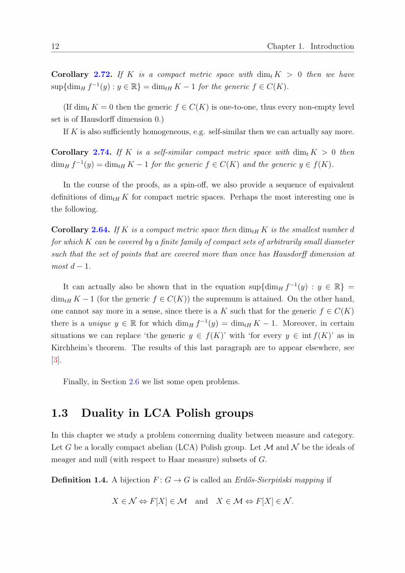
Corollary 2.72. If K is a compact metric space with dimtK > 0 then we have

sup{dimH f−1(y) : y ∈ R} = dimtH K − 1 for the generic f ∈ C(K).

(If dimtK = 0 then the generic f ∈ C(K) is one-to-one, thus every non-empty level

set is of Hausdorff dimension 0.)

If K is also sufficiently homogeneous, e.g. self-similar then we can actually say more.

Corollary 2.74. If K is a self-similar compact metric space with dimtK > 0 then

dimH f−1(y) = dimtH K − 1 for the generic f ∈ C(K) and the generic y ∈ f(K).

In the course of the proofs, as a spin-off, we also provide a sequence of equivalent

definitions of dimtH K for compact metric spaces. Perhaps the most interesting one is

the following.

Corollary 2.64. If K is a compact metric space then dimtH K is the smallest number d

for which K can be covered by a finite family of compact sets of arbitrarily small diameter

such that the set of points that are covered more than once has Hausdorff dimension at

most d− 1.

It can actually also be shown that in the equation sup{dimH f−1(y) : y ∈ R} =

dimtH K − 1 (for the generic f ∈ C(K)) the supremum is attained. On the other hand,

one cannot say more in a sense, since there is a K such that for the generic f ∈ C(K)

there is a unique y ∈ R for which dimH f−1(y) = dimtH K − 1. Moreover, in certain

situations we can replace ‘the generic y ∈ f(K)’ with ‘for every y ∈ int f(K)’ as in

Kirchheim’s theorem. The results of this last paragraph are to appear elsewhere, see

[3].

Finally, in Section 2.6 we list some open problems.

1.3 Duality in LCA Polish groups

In this chapter we study a problem concerning duality between measure and category.

Let G be a locally compact abelian (LCA) Polish group. Let M and N be the ideals of

meager and null (with respect to Haar measure) subsets of G.

Definition 1.4. A bijection F : G→ G is called an Erdos-Sierpinski mapping if

X ∈ N ⇔ F [X] ∈ M and X ∈ M ⇔ F [X] ∈ N .

1.4. The structure of rigid functions 13

Theorem 1.5 (Erdos–Sierpinski). Assume the Continuum Hypothesis. Then there ex-

ists an Erdos–Sierpinski mapping on R.

The existence of such a function is independent from ZFC. The main question of

Chapter 3 is the following:

Is it consistent that there is an Erdos–Sierpinski mapping F that preserves addition,

namely

∀x, y ∈ G F (x+ y) = F (x) + F (y)?

This question is attributed to Ryll-Nardzewski in the case G = R. Besides intrinsic

interest, another motivation was the following: If this statement were consistent then

the so called strong measure zero and strongly meager sets would consistently form

isomorphic ideals. (For the definitions see [9].)

First T. Bartoszynski [7] gave a negative answer to the question in the case G = 2ω,

then M. Kysiak proved this for G = R and answered the question of Ryll-Nardzewski,

see [26], where he used and improved Bartoszynski’s idea. We answer the general case,

the goal of Chapter 3 is to prove the following theorem:

Theorem 3.1. There is no addition preserving Erdos–Sierpinski mapping on any un-

countable locally compact abelian Polish group.

Let (φM) denote the following statement (considered by Carlson in [9]): For every

S ∈ M there exists a set S ′ ∈ M such that

∀x1, x2 ∈ G∃x ∈ G (S + x1) ∪ (S + x2) ⊆ S ′ + x.

Let (φN ) be the dual statement obtained by replacing M by N .

If there exists an Erdos–Sierpinski mapping preserving addition then (φM) and (φN )

are equivalent. In Section 3.2 we show that (φM) holds in LCA Polish groups. In Section

3.3 we begin to show that (φN ) fails for all uncountable LCA Polish groups by reducing

the general case to three special cases. Finally, in Section 3.4 we settle these three

special cases.

1.4 The structure of rigid functions

An easy calculation shows that the exponential function f(x) = ex has the somewhat

‘paradoxical’ property that cf(x) is a translate of f(x) for every c > 0. It is also easy

to see that every function of the form a + bekx has this property. This connection is

also of interest from the point of view of functional equations. Cain, Clark and Rose


[8] introduced the notion of vertical rigidity, which we now formulate for functions of

several variables.

Definition 4.1. A function f : Rd → R is called vertically rigid, if graph(cf) is isometric

to graph(f) for all c ∈ (0,∞). (Clearly, c ∈ R \ {0} would be the same.)

The main results of Chapter 4 are the characterizations of the continuous vertically

rigid functions of one and two variables. We need the following technical generalizations.

Definition 4.2. If C is a subset of (0,∞) and G is a set of isometries of Rd+1 then we

say that f is vertically rigid for a set C ⊆ (0,∞) via elements of G if for every c ∈ C

there exists a φ ∈ G such that φ (graph(f)) = graph(cf). (If we do not mention C or Gthen C is (0,∞) and G is the set of all isometries.)

In Section 4.1 we study the one-dimensional case. Clearly, every function of the form

a+ bx is vertically rigid. D. Jankovic conjectured (see [8]) that the converse is also true

for continuous functions.

Conjecture 4.3 (D. Jankovic). A continuous function f : R → R is vertically rigid if

and only if it is of the form a+ bx or a+ bekx (a, b, k ∈ R).

In Subsection 4.1.2 we prove Jankovic’s conjecture, even if we only assume that f is

a continuous vertically rigid function for an uncountable set C. (Later C. Richter [33]

proved a more general theorem.) We prove that if f is vertically rigid via translations,

then also weaker regularity of f implies Jankovic’s conjecture. In Subsection 4.1.3 we

show that Jankovic’s conjecture fails for Borel measurable functions. Our example also

answers a question from [8] that asks whether every vertically rigid function is of the

form a + bx or a + beg for some a, b ∈ R and additive function g. In Subsection 4.1.4

we prove that every Lebesgue (Baire) measurable function that is vertically rigid via

translations is of the form a+ bekx almost everywhere (on a co-meager set). The case of

general isometries remains open. We also prove that in many situations the exceptional

set can be removed. In Subsection 4.1.5 we define the notion of a rigid set, discuss how

it is connected to the notion of a rigid function, and prove an ergodic theory type result.

In Section 4.2 we look at the two-dimensional case. The characterization of the

continuous vertically rigid functions of two variables is the following.

Theorem 4.22. A continuous function f : R2 → R is vertically rigid if and only if after

a suitable rotation around the z-axis f(x, y) is of the form a + bx + dy, a + s(y)ekx or

a+ bekx + dy (a, b, d, k ∈ R, k = 0, s : R → R continuous).

1.4. The structure of rigid functions 15

The structure of the proof will be as follows. First we check in Subsection 4.2.2 that

functions of the above forms are rigid. (Of course, they are all continuous.) Then we

start proving Theorem 4.22 in more and more general settings.

In Subsection 4.2.3 first we show that if all the isometries are horizontal translations

then the vertically rigid function f(x, y) is of the form s(y)ekx (k ∈ R, k = 0, s : R → Rcontinuous). The punchline here is that we can derive a simple functional equation from

vertical rigidity (some sort of ‘multiplicativity’, see Lemma 4.9). Then we conclude this

subsection by a completely algebraic proof showing that if we allow arbitrary translations

then f(x, y) is of the form a+ s(y)ekx (a, k ∈ R, k = 0, s : R → R continuous). Then we

start working on the case of general isometries. The central idea is to consider the set Sf

of directions of segments connecting pairs of points on graph(f) (see Definition 4.30). We

collect the necessary properties of this set in Subsection 4.2.4. The set Sf has some sort

of rigidity in that the transformation f 7→ cf distorts the shape of it, but the resulting

set has to be isometric to the original one (see Definition 4.34 and Remark 4.35). Using

these we determine the possible Sf ’s in Subsection 4.2.5, then in Subsection 4.2.6 we

complete the proof by handling these cases using various methods.

In Section 4.3 we define the horizontally rigid functions, and characterize the func-

tions that are horizontally rigid via translations in dimension one. We do not assume

continuity, and analogous theorems hold in every dimension, see [4]. Later C. Richter

[33] proved that the continuous function f : R → R is horizontally rigid iff it is of the

form a + bx. M. Elekes and the author of this thesis proved in [4] that the continuous

function f : R2 → R is horizontally rigid iff it is of the form a + bx + dy. The problem

remains open in higher dimensions.

Finally, in Section 4.4 we collect the open questions of Chapter 4.

Chapter 2

The topological Hausdorff

dimension

2.1 Preliminaries

Let (X, d) be a metric space. We denote by clH, intH and ∂H the closure, interior

and boundary of a set H. For x ∈ X and H ⊆ X set d(x,H) = inf{d(x, h) : h ∈ H}.Let B(x, r) and U(x, r) stand for the closed and open ball of radius r centered at x,

respectively. More generally, for a set H ⊆ X we define B(H, r) = {x ∈ X : d(x,H) ≤r} and U(H, r) = {x ∈ X : d(x,H) < r}. The diameter of a set H is denoted

by diamH. We use the convention diam ∅ = 0. For two metric spaces (X, dX) and

(Y, dY ) a function f : X → Y is Lipschitz if there exists a constant C ∈ R such that

dY (f(x1), f(x2)) ≤ C · dX(x1, x2) for all x1, x2 ∈ X. The smallest such constant C is

called the Lipschitz constant of f and denoted by Lip(f). A function f : X → Y is

called bi-Lipschitz if f is a bijection and both f and f−1 are Lipschitz. Let X be a

metric space, s ≥ 0 and δ > 0, then

Hs∞(X) = inf

{∞∑i=1

(diamUi)s : X ⊆

∞∪i=1

Ui

},

Hsδ(X) = inf

{∞∑i=1

(diamUi)s : X ⊆

∞∪i=1

Ui,∀i diamUi ≤ δ

},

Hs(X) = limδ→0+

Hsδ(X).

The Hausdorff dimension of X is defined as

dimH X = inf{s ≥ 0 : Hs(X) = 0}.

17

18 Chapter 2. The topological Hausdorff dimension

For more information on these concepts see [14] or [29].

Let X be a complete metric space. A set is somewhere dense if it is dense in a

non-empty open set, and otherwise it is called nowhere dense. We say that M ⊆ X is

meager if it is a countable union of nowhere dense sets, and a set is called co-meager if

its complement is meager. By Baire’s Category Theorem co-meager sets are dense. It is

not difficult to show that a set is co-meager iff it contains a dense Gδ set. We say that the

generic element x ∈ X has property P , if {x ∈ X : x has property P} is co-meager. The

term ‘typical’ is also used instead of ‘generic’. Our two main examples will beX = C(K)

endowed with the supremum metric (for some compact metric space K) and X = K,

that is, a certain subspace of the non-empty compact subsets of Rd endowed with the

Hausdorff metric (i.e. dH(K1, K2) = min{r : K1 ⊆ B(K2, r) and K2 ⊆ B(K1, r)}). See

e.g. [23] for more on these concepts.

2.2 Basic properties of the topological Hausdorff di-

mension

Let X be a metric space. Since dimtX = −1 ⇐⇒ X = ∅ ⇐⇒ dimH X = −1, we

easily obtain

Fact 2.1. dimtH X = 0 ⇐⇒ dimtX = 0.

As dimH X is either −1 or at least 0, we obtain

Fact 2.2. The topological Hausdorff dimension of a non-empty space is either 0 or at

least 1.

These two facts easily yield

Corollary 2.3. Every metric space with a non-trivial connected component has topo-

logical Hausdorff dimension at least one.

The next theorem states that the topological Hausdorff dimension is between the

topological and the Hausdorff dimension.

Theorem 2.4. For every metric space X

dimtX ≤ dimtH X ≤ dimH X.

2.2. Basic properties of the topological Hausdorff dimension 19

Proof. We can clearly assume that X is non-empty. It is well-known that dimtX ≤dimH X (see e.g. [22]), which easily implies dimtX ≤ dimtH X using the definitions.

The second inequality is obvious if dimH X = ∞. If dimH X < 1 then dimtX = 0

(since dimtX ≤ dimH X and dimtX only takes integer values) and by Fact 2.1 we

obtain dimtH X = 0, hence the second inequality holds. Therefore we may assume that

1 ≤ dimH X < ∞. The following lemma is basically [29, Thm. 7.7.]. It is only stated

there in the special case X = A ⊆ Rn, but the proof works verbatim for all metric

spaces X.

Lemma 2.5. Let X be a metric space and f : X → Rm be Lipschitz. If s > m then∫ ⋆

Hs−m(f−1(y)

)dλm(y) ≤ c(m) Lip(f)mHs(X), (2.1)

where∫ ⋆

denotes the upper Lebesgue integral, λm the m-dimensional Lebesgue measure

and c(m) is a finite constant depending only on m.

Now we return to the proof of Theorem 2.4. We fix x0 ∈ X and define f : X → R by

f(x) = dX(x, x0). Using the triangle inequality it is easy to see that f is Lipschitz with

Lip(f) ≤ 1. We fix n ∈ N+ and apply Lemma 2.5 for f and s = dimH X + 1n> 1 = m.

Hence ∫ ⋆

Hs−1(f−1(y)) dλ1(y) ≤ c(1)Hs(X) = 0.

Thus Hs−1(f−1(y)) = HdimH X+ 1n−1(f−1(y)) = 0 holds for a.e. y ∈ R. Since this is true

for all n ∈ N+, we obtain that dimH f−1(y) ≤ dimH(X) − 1 for a.e. y ∈ R. From

the definition of f it follows that ∂U(x0, y) ⊆ f−1(y). Hence there is a neighborhood

basis of x0 with boundaries of Hausdorff dimension at most dimH(X) − 1, and this is

true for all x0 ∈ X, so there is a basis with boundaries of Hausdorff dimension at most

dimH(X) − 1. By the definition of the topological Hausdorff dimension this implies

dimtH X ≤ dimH X.

There are some elementary properties one expects from a notion of dimension. Now

we verify some of these for the topological Hausdorff dimension.

Extension of the classical dimension. Theorem 2.4 implies that the topological

Hausdorff dimension of a countable set equals zero, moreover, for open subspaces of Rd

and for smooth d-dimensional manifolds the topological Hausdorff dimension equals d.

Monotonicity. Let X ⊆ Y . If U is a basis in Y then UX = {U ∩X : U ∈ U} is a

basis in X, and ∂X(U ∩X) ⊆ ∂YU holds for all U ∈ U . This yields


Fact 2.6 (Monotonicity). If X ⊆ Y are metric spaces then dimtH X ≤ dimtH Y .

Bi-Lipschitz invariance. First we prove that the topological Hausdorff dimen-

sion does not increase under Lipschitz homeomorphisms. An easy consequence of this

that our dimension is bi-Lipschitz invariant, and does not increase under an injective

Lipschitz map on a compact space. After obtaining corollaries of Theorem 2.7 we give

some examples illustrating the necessity of certain conditions in this theorem and its

corollaries.

Theorem 2.7. Let X, Y be metric spaces. If f : X → Y is a Lipschitz homeomorphism

then dimtH Y ≤ dimtH X.

Proof. Since f is a homeomorphism, if U is a basis in X then V = {f(U) : U ∈ U} is

a basis in Y , and ∂f(U) = f(∂U) for all U ∈ U . The Lipschitz property of f implies

that dimH ∂V = dimH ∂f(U) = dimH f(∂U) ≤ dimH ∂U for all V = f(U) ∈ V . Thus

dimtH Y ≤ dimtH X.

This immediately implies the following two statements.

Corollary 2.8 (Bi-Lipschitz invariance). Let X, Y be metric spaces. If f : X → Y is

bi-Lipschitz then dimtH X = dimtH Y .

Corollary 2.9. If K is a compact metric space, and f : K → Y is one-to-one Lipschitz

then dimtH f(K) ≤ dimtH K.

The following example shows that we cannot drop injectivity here. First we need a

well-known lemma.

Lemma 2.10. Let M ⊆ R be measurable with positive Lebesgue measure. Then there

exists a Lipschitz onto map f : M → [0, 1].

Proof. Let us choose a compact set C ⊆ M of positive Lebesgue measure. Define

f : M → [0, 1] by

f(x) =λ ((−∞, x) ∩ C)

λ(C),

where λ denotes the one-dimensional Lebesgue measure. Then it is not difficult to see

that f is Lipschitz (with Lip(f) ≤ 1λ(C)

) and f(C) = [0, 1].

Example 2.11. Let K ⊆ R be a Cantor set (that is, a set homeomorphic to the middle-

thirds Cantor set) of positive Lebesgue measure. By Fact 2.1, dimtH K = dimtK = 0.

Using Lemma 2.10 there is a Lipschitz map f : K → [0, 1] such that f(K) = [0, 1]. By

Theorem 2.4, dimtH [0, 1] = 1, hence dimtH K = 0 < 1 = dimtH [0, 1] = dimtH f(K).


The next example shows that Corollary 2.9 does not hold without the assumption

of compactness. We even have a separable metric counterexample.

Example 2.12. Let C be the middle-thirds Cantor set, and f : C×C → [0, 2] be defined

by f(x, y) = x+ y. It is well-known and easy to see that f is Lipschitz and f(C ×C) =

[0, 2]. Therefore one can select a subset X ⊆ C × C such that f |X is a bijection from

X onto [0, 2]. Then X is separable metric. Monotonicity and dimt(C × C) = 0 imply

dimtH X ≤ dimtH(C × C) = 0. Therefore, f is one-to-one and Lipschitz on X but

dimtH X = 0 < 1 = dimtH [0, 2] = dimtH f(X).

Our last example shows that the topological Hausdorff dimension is not invariant

under homeomorphisms. Not even for compact metric spaces.

Example 2.13. Let C1, C2 ⊆ R be Cantor sets such that dimH C1 = dimH C2. We will

see in Theorem 2.19 that dimtH(Ci× [0, 1]) = dimH Ci+1 for i = 1, 2. Hence C1× [0, 1]

and C2 × [0, 1] are homeomorphic compact metric spaces whose topological Hausdorff

dimensions disagree.

Stability and countable stability. As the following example shows, similarly to

the case of topological dimension, stability does not hold for non-closed sets. That is,

X =∪k

n=1Xn does not imply dimtH X = max1≤n≤k dimtH Xn.

Example 2.14. Theorem 2.4 implies dimtH(R) = 1, and Fact 2.1 yields dimtH(Q) =

dimt(Q) = 0 and dimtH(R \ Q) = dimt(R \ Q) = 0. Thus dimtH R = 1 > 0 =

max{dimtH(Q), dimtH(R \Q)}, and therefore stability fails.

As a corollary, we now show that as opposed to the case of Hausdorff (and packing)

dimension, there is no reasonable family of measures inducing the topological Hausdorff

dimension. Let us say that a 1-parameter family of measures {µs}s≥0 is monotone if

µs(A) = 0, s < t implies µt(A) = 0. The family of Hausdorff (or packing) measures

certainly satisfies this criterion. It is not difficult to see that monotonicity implies that

the induced notion of dimension, that is, dimA = inf{s : µs(A) = 0} is countably stable.

Hence we obtain

Corollary 2.15. There is no monotone 1-parameter family of measures {µs}s≥0 such

that dimtH A = inf{s : µs(A) = 0}.

However, just like in the case of topological dimension, even countable stability holds

for closed sets.


Theorem 2.16 (Countable stability for closed sets). Let X be a separable metric space

and X =∪

n∈N Xn, where Xn (n ∈ N) are closed subsets of X. Then dimtH X =

supn∈N dimtH Xn.

Proof. Monotonicity clearly implies dimtH X ≥ supn∈N dimtH Xn. For the other direc-

tion we may assume supn∈N dimtH Xn < ∞. Let d > supn∈N dimtH Xn be arbitrary.

Assume Un, n ∈ N is a countable basis of Xn such that dimH ∂XnU ≤ d − 1 for all

n ∈ N and U ∈ Un. Let Y =∪{∂XnU : n ∈ N, U ∈ Un}. By countable stability of the

Hausdorff dimension, dimH Y ≤ d−1. Using the definition of the topological dimension

we obtain dimt(Xn \ Y ) = 0 for all n ∈ N. The set Xn \ Y is closed in the separable

metric space X \ Y , and X \ Y =∪

n∈N(Xn \ Y ). By the sum theorem for topological

dimension 0, see [12, 1.3.1], dimt(X \ Y ) = 0.

Let us fix an open set V ⊆ X and a point x ∈ V . Using that X \ Y is a separable

subspace of X with topological dimension 0, by the separation theorem for topological

dimension zero [12, 1.2.11.] there is a so-called partition between x and X \ V disjoint

from X \ Y . This means that there exist disjoint open sets U,U ′ ⊆ X such that x ∈ U ,

X \ V ⊆ U ′ and (X \ (U ∪ U ′)) ∩ (X \ Y ) = ∅. In particular, x ∈ U ⊆ V . Moreover,

∂XU ∩ (X \ Y ) = ∅, so ∂XU ⊆ Y , thus dimH ∂XU ≤ dimH Y ≤ d− 1. By the definition

of topological Hausdorff dimension we obtain dimtH X ≤ d. As d > supn∈N dimtH Xn

was arbitrary, the proof is complete.

Corollary 2.17. The same holds for Fσ sets, as well.

Products. Now we investigate products from the point of view of topological Haus-

dorff dimension. By product of two metric spaces we will always mean the l2-product,

that is,

dX×Y ((x1, y1), (x2, y2)) =√d2X(x1, x2) + d2Y (y1, y2).

First we recall a well-known statement, see [14, Chapters 3 and 7] for the definitions

and the proof.

Lemma 2.18. Let X, Y be non-empty metric spaces such that dimH Y = dimBY , where

dimB is the upper box-counting dimension. Then

dimH(X × Y ) = dimH X + dimH Y.

Now we prove our next theorem which provides a large class of sets for which the

topological Hausdorff dimension and the Hausdorff dimension coincide.


Theorem 2.19. Let X be a non-empty separable metric space. Then

dimtH (X × [0, 1]) = dimH (X × [0, 1]) = dimH X + 1.

Proof. Applying Lemma 2.18 for Y = [0, 1] we obtain dimH (X × [0, 1]) = dimH X +

dimH [0, 1] = dimH X + 1. In addition, Theorem 2.4 follows that dimtH (X × [0, 1]) ≤dimH (X × [0, 1]). For the opposite inequality we need the following lemma.

Lemma 2.20. Let X be a non-empty separable metric space and let d < dimH X be

fixed. Then there exists xd ∈ X such that dimH U(xd, r) ≥ d holds for every r > 0.

Proof of the Lemma. Assume, on the contrary, that for all x ∈ X there is an rx > 0

such that dimH U(x, rx) < d. Since X is separable, by the Lindelof property we can

select a countable subcover {U(xn, rn)}n∈N of the cover {U(x, rx)}x∈X . By countable

stability of the Hausdorff dimension dimH X = supn∈N dimH U(xn, rn) ≤ d, which is a

contradiction.

We now return to the proof of Theorem 2.19. For a fixed d < dimH X assume that

xd ∈ X is given as in the lemma. Let U be a basis in X× [0, 1] and prX : X× [0, 1] → X,

prX(x, y) = x. There exists Ud ∈ U such that (xd, 1) ∈ Ud and Ud ∩(X ×

[0, 1

2

])= ∅.

Then there is an rd > 0 such that U(xd, rd) × [1 − rd, 1] ⊆ Ud. For every x ∈ U(xd, rd)

we have (x, 0) /∈ Ud and (x, 1) ∈ Ud, hence ∂Ud ∩ (x × [0, 1]) = ∅. Thus U(xd, rd) ⊆prX(∂Ud). Projections do not increase the Hausdorff dimension, therefore dimH ∂Ud ≥dimH U(xd, rd) ≥ d. This is valid for all d < dimH X, so supU∈U dimH ∂U ≥ dimH X

for all basis U , thus dimtH(X × [0, 1]) ≥ dimH X + 1 by the definition of topological

Hausdorff dimension.

Remark 2.21. We cannot drop separability here. Indeed, if X is an uncountable

discrete metric space then it is not difficult to see that dimtH(X × [0, 1]) = 1 and

dimH(X × [0, 1]) = dimH X = ∞.

Separability is a rather natural assumption throughout the chapter. First, the Haus-

dorff dimension is only meaningful in this context (it is always infinite for non-separable

spaces), secondly for the theory of topological dimension this is the most usual frame-

work.

Corollary 2.22. If X is a non-empty separable metric space then

dimtH

(X × [0, 1]d

)= dimH

(X × [0, 1]d

)= dimH X + d.


The possible values of (dimtX, dimtH X, dimH X).

The following theorem provides a complete description of the possible values of

the triple (dimtX, dimtH X, dimH X). Moreover, all possible values can be realized by

compact spaces as well.

Theorem 2.23. For a triple (d, s, t) ∈ [0,∞]3 the following are equivalent.

(i) There exists a compact metric space K such that dimtK = d, dimtH K = s, and

dimH K = t.

(ii) There exists a separable metric space X such that dimtX = d, dimtH X = s, and

dimH X = t.

(iii) There exists a metric space X such that dimtX = d, dimtH X = s, and dimH X =

t.

(iv) d = s = t = −1, or d = s = 0, t ∈ [0,∞], or d ∈ N+ ∪ {∞}, s, t ∈ [1,∞], d ≤s ≤ t.

Proof. The implications (i) =⇒ (ii) and (ii) =⇒ (iii) are obvious, and (iii) =⇒ (iv)

can easily be checked using Fact 2.1 and Theorem 2.4.

It remains to prove that (iv) =⇒ (i). First, the empty set takes care of the case

d = s = t = −1. Let now d = s = 0, t ∈ [0,∞]. For t ∈ [0,∞] let Kt be a Cantor set

with dimH Kt = t. Such sets are well-known to exist already in [0, 1]n for large enough

n in case t <∞, whereas if C is the middle-thirds Cantor set then CN is such a set for

t = ∞. Then clearly dimtKt = dimtH Kt = 0 and dimH Kt = t, so we are done with

this case.

Finally, let d ∈ N+ ∪ {∞}, s, t ∈ [1,∞], d ≤ s ≤ t. We may assume d < ∞,

otherwise the Hilbert cube provides a suitable example. (Indeed, clearly dimt[0, 1]N =

dimtH [0, 1]N = dimH [0, 1]

N = ∞.) Define Kd,s,t = (Ks−d × [0, 1]d) ∪ Kt (this can be

understood as the disjoint sum of metric spaces, but we may also assume that all

these spaces are in the Hilbert cube, so the union is well defined). Since dimt(X ×Y ) ≤ dimtX + dimt Y for non-empty spaces (see e.g. [12]), we obtain dimt(Ks−d ×[0, 1]d) = 0+ d = d. Hence, by the stability of the topological dimension for closed sets,

dimtKd,s,t = max{dimt

(Ks−d × [0, 1]d

), dimtKt

}= max{d, 0} = d. Using Corollary

2.22 and the stability of the topological Hausdorff dimension for closed sets we infer

that dimtH Kd,s,t = max{dimtH

(Ks−d × [0, 1]d

), dimtH Kt

}= max{s − d + d, 0} = s.

Again by Corollary 2.22 and by the stability of the Hausdorff dimension we obtain that

2.3. Calculating the topological Hausdorff dimension 25

dimH Kd,s,t = max{dimH

(Ks−d × [0, 1]d

), dimH Kt

}= max{s−d+d, t} = max{s, t} =

t. This completes the proof.

The topological Hausdorff dimension is not a function of the topological

and the Hausdorff dimension.

As a particular case of the above theorem we obtain that there are compact metric

spaces X and Y such that dimtX = dimt Y and dimH X = dimH Y but dimtH X =dimtH Y . This immediately implies the following, which shows that the topological

Hausdorff dimension is indeed a genuinely new concept.

Corollary 2.24. dimtH X cannot be calculated form dimtX and dimH X, even for

compact metric spaces.

2.3 Calculating the topological Hausdorff dimension

2.3.1 Some classical fractals

First we present certain natural examples of compact sets K with dimtK = dimtH K <

dimH K. Let S be the Sierpinski triangle, then it is well-known that dimt S = 1 and

dimH S = log 3log 2

.

Theorem 2.25. Let S be the Sierpinski triangle. Then dimtH(S) = 1.

Proof. Let φi : R2 → R2 (i = 1, 2, 3) be the three similitudes with ratio 1/2 for which

S =∪3

i=1 φi(S). Sets of the form φin ◦ · · · ◦ φi1(S), n ∈ N, j ∈ {1, . . . , n}, ij ∈ {1, 2, 3}are called the elementary pieces of S. It is not difficult to see that

U = {intS H : H is a finite union of elementary pieces of S}

is a basis of S such that #∂SU is finite for every U ∈ U . Therefore dimH ∂SU ≤ 0,

and hence dimtH S ≤ 1. On the other hand, S contains a line segment, therefore

dimtH S ≥ dimtH [0, 1] = 1 by monotonicity.

Now we turn to the von Koch snowflake curve K. Recall that dimtK = 1 and

dimH K = log 4log 3

.

Fact 2.26. If K is homeomorphic to [0, 1] then dimtH K = 1.

Proof. By Corollary 2.3 we obtain that dimtH K ≥ 1. On the other hand, since K is

homeomorphic to [0, 1], there is a basis in K such that #∂U ≤ 2 for every U ∈ U . ThusdimtH K ≤ 1.


Corollary 2.27. Let K be the von Koch curve. Then dimtH K = 1.

Next we take up a natural example of a compact set K with dimtK < dimtH K <

dimH K. Let T be the Sierpinski carpet, then it is well-known that dimt T = 1 and

dimH T = log 8log 3

.

Theorem 2.28. Let T be the Sierpinski carpet. Then dimtH(T ) =log 2log 3

+ 1 = log 6log 3

.

Proof. Let C denote the middle-thirds Cantor set. Observe that C × [0, 1] ⊆ T . Then

monotonicity and Theorem 2.19 yield dimtH T ≥ dimtH(C × [0, 1]) = dimH C + 1 =log 2log 3

+ 1.

Let us now prove the opposite inequality. For n ∈ N and i = 1, . . . , 3n let zni = 2i−12(3n)

.

Then clearly

{zni : n ∈ N, i ∈ {1, . . . , 3n}}

is dense in [0, 1]. Let L be a horizontal line defined by an equation of the form y = zni

or a vertical line defined by x = zni . It is easy to see that L∩T consists of finitely many

sets geometrically similar to the middle-thirds Cantor set. Using these lines it is not

difficult to construct a rectangular basis U of T such that dimH ∂TU = log 2log 3

for every

U ∈ U , and hence dimtH T ≤ log 2log 3

+ 1.

Finally we remark that, by Theorem 2.19, K = C × [0, 1] (where C is the middle-

thirds Cantor set) is a natural example of a compact set with dimtK < dimtH K =

dimH K.

2.3.2 Kakeya sets

Definition 2.29. A subset of Rd is called a Kakeya set if it contains a non-degenerate

line segment in every direction (some authors call these sets Besicovitch sets).

According to a surprising classical result, Kakeya sets of Lebesgue measure zero exist.

However, one of the most famous conjectures in analysis is the Kakeya Conjecture stating

that every Kakeya set in Rd has Hausdorff dimension d. This is known to hold only in

dimension at most 2 so far, and a solution already in R3 would have a huge impact on

numerous areas of mathematics.

It would be tempting to attack the Kakeya Conjecture using dimtH K ≤ dimH K,

but the following theorem, the main theorem of this section will show that unfortunately

we cannot get anything non-trivial this way.

Theorem 2.30. There exists a Kakeya set K ⊆ Rd of topological Hausdorff dimension

1 for every integer d ≥ 1.

2.3. Calculating the topological Hausdorff dimension 27

This result is of course sharp, since if a set contains a line segment then its topological

Hausdorff dimension is at least 1.

We will actually prove somewhat more, since we will essentially show that the generic

element of a carefully chosen space is a Kakeya set of topological Hausdorff dimension

1. This idea, as well as most of the others in this subsection are already present in [25]

by T. W. Korner. However, he only works in the plane and his space slightly differs

from ours. For the sake of completeness we provide the rather short proof details.

Let (K, dH) be the set of compact subsets of Rd−1× [0, 1] endowed with the Hausdorff

metric, that is for each K1, K2 ∈ K

dH(K1, K2) = min {r : K1 ⊆ B(K2, r) and K2 ⊆ B(K1, r)} ,

where B(K, r) ={x ∈ Rd−1 × [0, 1] : dist(x,K) ≤ r

}. It is well-known that (K, dH) is a

complete metric space, see e.g. [23].

Let

Γ = {(x1, . . . , xd−1, 1) : 1/2 ≤ xi ≤ 1, i = 1, . . . , d− 1}

denote a subset of directions in Rd. A closed line segment w connecting Rd−1×{0} and

Rd−1 × {1} is called a standard segment.

Let us denote by F ⊆ K the system of those compact sets in Rd−1 × [0, 1] in which

for each v ∈ Γ we can find a standard segment w parallel to v. First we show that Fis closed in K. Let us assume that Fn ∈ F , K ∈ K and Fn → K with respect to dH .

We have to show that K ∈ F . Let v ∈ Γ be arbitrary. Since Fn ∈ F , there exists a

wn ⊆ Fn parallel to v for every n. It is easy to see that∪

n∈N Fn is bounded, hence

we can choose a subsequence nk such that wnkis convergent with respect to dH . But

then clearly wnk→ w for some standard segment w ⊆ K, and w is parallel to v. Hence

K ∈ F indeed.

Therefore, (F , dH) is a complete metric space and hence we can use Baire category

arguments.

The next lemma is based on [25, Thm. 3.6.].

Lemma 2.31. The generic set in (F , dH) is of topological Hausdorff dimension 1.

Proof. The rational cubes form a basis of Rd, and their boundaries are covered by the

rational hyperplanes orthogonal to one of the usual basis vectors of Rd. Therefore, it

suffices to show that if S is a fixed hyperplane orthogonal to one of the usual basis

vectors then {F ∈ F : dimH(F ∩ S) = 0} is co-meager.


For n ∈ N+ define

Fn =

{F ∈ F : H

1n1n

(F ∩ S) < 1

n

}.

In order to show that {F ∈ F : dimH(F ∩ S) = 0} =∩

n∈N+ Fn is co-meager, it is

enough to prove that each Fn contains a dense open set.

For p ∈ Rd, v ∈ Γ and 0 < α < π/2 we denote by C(p, v, α) the following doubly

infinite closed cone

C(p, v, α) = {x ∈ Rd : the angle between the lines of v and x− p is at most α}.

We denote by V (C(p, v, α)) the set of those vectors u = (u1, ..., ud−1, 1) for which there

is a line in int(C(p, v, α)) ∪ {p} parallel to u. Then V (C(p, v, α)) is relatively open in

Rd−1 × {1}.The sets of the form C ′(p, v, α) = C(p, v, α)∩

(Rd−1 × [0, 1]

)will be called truncated

cones, and the system of truncated cones will be denoted by C ′. A truncated cone

C ′(p, v, α) is S-compatible if either C ′(p, v, α) ∩ S = {p}, or C ′(p, v, α) ∩ S = ∅. Theset of S-compatible truncated cones is denoted by C ′

S. Define FS as the set of those

F ∈ F that can be written as the union of finitely many S-compatible truncated cones

and finitely many points in Rd−1 × [0, 1].

Next we check that FS is dense in F .

Suppose F ∈ F is arbitrary and ε > 0 is given. First choose finitely many points

{yi}ti=1 in F such that F ⊆ B ({yi}ti=1, ε). Let v ∈ Γ be arbitrary, then there exists a

standard segment wv ⊆ F parallel to v. By the choice of S and Γ, clearly wv * S, hence

we can choose pv and αv such that C ′(pv, v, αv) ∈ C ′S and dH(C

′(pv, v, αv), wv) ≤ ε. Ob-

viously v ∈ V (C(pv, v, αv)), so {V (C(pv, v, αv))}v∈Γ is an open cover of the compact set

Γ. Therefore, there are {C ′(pvi , vi, αvi)}mi=1 in C ′S such that Γ ⊆

∪mi=1 V (C(pvi , vi, αvi)).

Put F ′ =∪m

i=1C′(pvi , vi, αvi) ∪ {y1, . . . , yt}, then F ′ ∈ FS. It is easy to see that∪m

i=1C′(pvi , vi, αvi) ⊆ B(F, ε), and combining this with {yi}ti=1 ⊆ F we obtain that

F ′ ⊆ B(F, ε). By the choice of {yi}ti=1 we also have F ⊆ B(F ′, ε). Thus dH(F, F′) ≤ ε.

Now using our dense set FS we verify that Fn contains a dense open set U . We

construct for all F0 ∈ FS a ball in Fn centered at F0. By the definition of S-compatibility

F0 ∩ S is finite. Hence we can easily choose a relatively open set U0 ⊆ S such that

F0 ∩ S ⊆ U0 and H1n1n

(U0) <1n. Let us define

U = {F ∈ F : F ∩ S ⊆ U0} .

Clearly F0 ∈ U , U ⊆ Fn and it is easy to see that U is open in F . This completes the

proof.

2.4. Application I: Mandelbrot’s fractal percolation process 29

From this we obtain the main theorem of the section as follows.

Proof of Theorem 2.30. The above lemma implies that we can choose F0 ∈ F such

that dimtH F0 = 1. Then F0 contains a line segment in every direction of Γ, hence

we can choose finitely many isometric copies of it, {Fi}ni=1 such that the compact set

K =∪n

i=0 Fi contains a line segment in every direction. By the Lipschitz invariance of

the topological Hausdorff dimension dimtH Fi = dimtH F0 for all i, and by the stability

of the topological Hausdorff dimension for closed sets dimtH K = 1.

2.3.3 Brownian motion

One of the most important stochastic processes is the Brownian motion (see e.g. [30]).

Its trail and graph also serve as important examples of fractal sets in geometric measure

theory. Since the graph is always homeomorphic to [0,∞), Fact 2.26 and countable

stability for closed sets yield that its topological Hausdorff dimension is 1. Hence we

focus on the trail only.

Each statement in this paragraph is to be understood to hold with probability 1

(almost surely). Clearly, in dimension 1 the trail is a non-degenerate interval, so it has

topological Hausdorff dimension 1. Moreover, if the dimension is at least 4 then the trail

has no multiple points ([30]), so it is homeomorphic to [0,∞), which in turn implies as

above that the trail has topological Hausdorff dimension 1 again. However, the following

question is open.

Problem 2.32. Let d = 2 or 3. Determine the almost sure topological Hausdorff di-

mension of the trail of the d-dimensional Brownian motion.

2.4 Application I: Mandelbrot’s fractal percolation

process

In this section we take up one of the most important random fractals, the limit set M

of the fractal percolation process defined by Mandelbrot in [28].

His original motivation was that this model captures certain features of turbulence,

but then this random set turned out to be very interesting in its own right. For example,

M serves as a very powerful tool for calculating Hausdorff dimension. Indeed, J. Hawkes

has shown ([19]) that for a fixed Borel set B in the unit square (or analogously in higher

dimensions) M ∩ B = ∅ almost surely iff the sum of the co-dimensions exceeds 2,

(that is, (2 − dimH M) + (2 − dimH B) > 2), and this formula can be used in certain


applications to determine dimH B. Moreover, it can be shown that the trail of the

Brownian motion is so called intersection-equivalent to a percolation fractal (roughly

speaking, they intersect the same sets with positive probability), and this can be used to

deduce numerous dimension related results about the Brownian motion, see the works

of Y. Peres, e.g. in [30].

Let us now formally describe the fractal percolation process. Let p ∈ (0, 1) and n ≥ 2,

n ∈ N be fixed. SetM0 =M(p,n)0 = [0, 1]2. We divide the unit square into n2 equal closed

subsquares of side-length 1/n in the natural way. We keep each subsquare independently

with probability p (and erase it with probability 1 − p), and denote by M1 = M(p,n)1

the union of the kept subsquares. Then each square in M1 is divided into n2 squares of

side-length 1/n2, and we keep each of them independently (and also independently of

the earlier choices) with probability p, etc. After k steps let Mk = M(p,n)k be the union

of the kept kth level squares with side-length 1/nk. Let

M =M (p,n) =∞∩k=1

Mk. (2.2)

The process we have just described is called Mandelbrot’s fractal percolation process,

and M is called its limit set.

Percolation fractals are not only interesting from the point of view of turbulence

and fractal geometry, but they are also closely related to the (usual, graph-theoretic)

percolation theory. In case of the fractal percolation the role of the clusters is played by

the connected components. Our starting point will be the following celebrated theorem.

Recall that a space is totally disconnected if every connected component is a singleton.

Theorem 2.33 (Chayes-Chayes-Durrett, [10]). There exists a critical probability pc =

p(n)c ∈ (0, 1) such that if p < pc then M is totally disconnected almost surely, and if

p > pc then M contains a nontrivial connected component with positive probability.

They actually prove more, the most powerful version states that in the supercritical

case (i.e. when p > pc) there is actually a unique unbounded component if the process

is extended to the whole plane, but we will only concentrate on the most surprising fact

that the critical probability is strictly between 0 and 1.

The main goal of the present section will be to prove the following generalization of

the above theorem.

Theorem 2.34. For every d ∈ [0, 2) there exists a critical probability p(d)c = p

(d,n)c ∈

(0, 1) such that if p < p(d)c then dimtH M ≤ d almost surely, and if p > p

(d)c then

dimtH M > d almost surely (provided M = ∅).


In order to see that we actually obtain a generalization, just note that a compact

space is totally disconnected iff dimtM = 0 ([12]), also that dimtH M = 0 iff dimtM = 0,

and use d = 0. Theorem 2.33 basically says that certain curves show up at the critical

probability, and our proof will show that even ‘thick’ families of curves show up, where

the word thick is related to large Hausdorff dimension.

In the rest of this section first we do some preparations in the first subsection, then

we prove the main theorem (Theorem 2.34) in the next subsection, and finally give an

upper bound for dimtH M and conclude that dimtH M < dimH M almost surely in the

non-trivial cases.

2.4.1 Preparation

For the proofs of the statements in the next two remarks see e.g. [10].

Remark 2.35. It is well-known from the theory of branching processes that M = ∅almost surely iff p ≤ 1

n2 , so we may assume in the following that p > 1n2 .

If 1n2 < p ≤ 1√

nthen dimtM = 0 almost surely. Hence Fact 2.1 implies that

dimtH M = 0 almost surely. (In fact, the same holds even for p < pc, see Theorem 2.33.)

Remark 2.36. As for the Hausdorff dimension, for p > 1n2 we have

dimH M = 2 +log p

log n

almost surely, provided M = ∅.We will also need the 1-dimensional analogue of the process (intervals instead of

squares). Here M (1D) = ∅ almost surely iff p ≤ 1n, and for p > 1

nwe have

dimH M(1D) = 1 +

log p

log n

almost surely, provided M (1D) = ∅.

Now we check that the almost sure topological Hausdorff dimension ofM also exists.

Lemma 2.37. For every p > 1n2 and n ≥ 2, n ∈ N there exists a number d = d(p,n) ∈

[0, 2] such that

dimtH M = d

almost surely, provided M = ∅.


Proof. Let N be the random number of squares in M1. Let us set q = P (M = ∅). Thenq < 1 by p > 1

n2 , and [14, Thm. 15.2] gives that q is the least positive root of the

polynomial

f(t) = −t+n2∑k=0

P (N = k)tk.

First we show that P (dimtH M ≤ x) is a root of f for every x ∈ R.Let M1 = {Q1, . . . , QN}, where the Qi’s are the first level subsquares, and fix x ∈ R.

(Define Q1 = ∅ if N = 0.) For every i and k let MQi

k be the union of those squares in

Mk that are in Qi, and let MQi =∩

kMQi

k . (Note that this is not the same as M ∩Qi,

since in this latter set there may be points on the boundary of Qi ‘coming from squares

outside of Qi’.) Then MQi has the same distribution as a similar copy of M (this is

called statistical self-similarity), and hence for every i

P(dimtH M

Qi ≤ x)= P (dimtH M ≤ x) .

Using the stability of the topological Hausdorff dimension for closed sets and the fact

that the MQi ’s are independent and have the same distribution under the condition

N = k, this implies

P (dimtH M ≤ x |N = k) = P(dimtH M

Qi ≤ x for each 1 ≤ i ≤ k |N = k)

=(P(dimtH M

Q1 ≤ x) )k

=(P (dimtH M ≤ x)

)k.

Therefore, we obtain

P (dimtH M ≤ x) =n2∑k=0

P (N = k)P (dimtH M ≤ x |N = k)

=n2∑k=0

P (N = k)(P (dimtH M ≤ x)

)k,

and thus P (dimtH M ≤ x) is indeed a root of f for every x.

As mentioned above, q = 1 and q is also a root of f . Moreover, 1 is obviously also

a root, and it is easy to see that f is strictly convex on (0,∞), hence there are at most

two positive roots. Hence q and 1 are the only roots, therefore P (dimtH M ≤ x) = q or

1 for every x.

Then the distribution function F (x) = P (dimtH M ≤ x |M = ∅) only attains the

values 0 and 1, moreover, F (0) = 0, F (2) = 1, thus there is a value d where it ‘jumps’

from 0 to 1, and this concludes the proof.


2.4.2 Proof of Theorem 2.34; the lower estimate of dimtH M

Set

p(d,n)c = sup{p : dimtH M

(p,n) ≤ d almost surely}.

First we need some lemmas. The following one is analogous to [17, p. 387].

Lemma 2.38. For every d ∈ R and n ∈ N, n ≥ 2

p(d,n)c < 1 ⇐⇒ p(d,n2)

c < 1.

Proof. Clearly, it is enough to show that

p(d,n)c

(1−

(1− p(d,n)c

) 1n2

)≤ p(d,n

2)c ≤ p(d,n)c . (2.3)

We say that the random construction X is dominated by the random construction Y if

they can be realized on the same probability space such that X ⊆ Y almost surely.

Let us first prove the second inequality in (2.3). It clearly suffices to show that

dimtH M(p,n2) ≤ d almost surely =⇒ dimtH M

(p,n) ≤ d almost surely.

But this is rather straightforward, since M(p,n)2k is easily seen to be dominated byM

(p,n2)k

for every k, hence M (p,n) is dominated by M (p,n2).

Let us now prove the first inequality in (2.3). Set φ(x) = 1 − (1− x)1/n2

. We need

to show that

0 < p < p(d,n)c φ(p(d,n)c ) =⇒ dimtH M(p,n2) ≤ d almost surely. (2.4)

Since xφ(x) is an increasing homeomorphism of the unit interval, p = qφ(q) for some

q ∈ (0, 1). Then clearly q < p(d,n)c , so dimtH M

(q,n) ≤ d almost surely. Therefore, in order

to prove (2.4) it suffices to check that

M (p,n2) is dominated by M (q,n). (2.5)

First we check that

M(φ(q),n2)k is dominated by M

(q,n)k for every k, (2.6)

and consequently M (φ(q),n2) is dominated by M (q,n). Indeed, in the second case we erase

a subsquare of side length 1nwith probability 1−q and keep it with probability q, while in

the first case we completely erase a subsquare of side length 1nwith the same probability

(1− φ(q))n2= 1− q and hence keep at least a subset of it with probability q.


But this will easily imply (2.5), which will complete the proof. Indeed, after each

step of the processes M (φ(q),n2) and M (q,n) let us perform the following procedures. For

M (φ(q),n2) let us keep every existing square independently with probability q and erase

it with probability 1 − q (we do not do any subdivisions in this case). For M (q,n) let

us take one more step of the construction of M (q,n). Using (2.6) this easily implies that

M(qφ(q),n2)k is dominated by M

(q,n)2k for every k, hence M (qφ(q),n2) is dominated by M (q,n),

but qφ(q) = p, and hence (2.5) holds.

From now on let N be a fixed (large) positive integer to be chosen later. Recall that

a square of level k is a set of the form[

iNk ,

i+1Nk

]×[

jNk ,

j+1Nk

]⊆ [0, 1]2.

Definition 2.39. A walk of level k is a sequence (S1, . . . , Sl) of non-overlapping squares

of level k such that Sr and Sr+1 are abutting for every r = 1, . . . , l − 1, moreover

S1 ∩ ({0} × [0, 1]) = ∅ and Sl ∩ ({1} × [0, 1]) = ∅.

In particular, the only walk of level 0 is ([0, 1]2).

Definition 2.40. We say that (S1, . . . , Sl) is a turning walk (of level 1) if it satisfies the

properties of a walk of level 1 except that instead of Sl ∩ ({1} × [0, 1]) = ∅ we require

that Sl ∩ ([0, 1]× {1}) = ∅.

Lemma 2.41. Let S be a set of N−2 distinct squares of level 1 intersecting {0}× [0, 1],

and let T be a set of N −2 distinct squares of level 1 intersecting {1}× [0, 1]. Moreover,

let F ∗ be a square of level 1 such that the row of F ∗ does not intersect S ∪ T . Then

there exist N − 2 non-overlapping walks of level 1 not containing F ∗ such that the set

of their first squares coincides with S and the set of their last squares coincides with T .

Case 1. Case 2. Case 3.

Figure 2.1: Illustration to Lemma 2.41


Proof. The proof is by induction on N . The case N = 2 is obvious.

Case 1. F ∗ is in the top or bottom row.

By simply ignoring this row it is straightforward how to construct the walks in the

remaining rows.

Case 2. F ∗ is not in the top or bottom row, and both top corners or both bottom corners

are in S ∪ T .

Without loss of generality we may suppose that both top corners are in S ∪ T . Let

the straight walk connecting these two corners be one of the walks to be constructed.

Then let us shift the remaining members of T to the left by one square, and either we

can apply the induction hypothesis to the (N−1)×(N−1) many squares in the bottom

left corner of the original N×N many squares, or F ∗ is not among these (N−1)×(N−1)

many squares and then the argument is even easier. Then one can see how to get the

required walks.

Case 3. Neither Case 1 nor Case 2 holds.

Since there are only two squares missing on both sides, and F ∗ cannot be the top or

bottom row, we infer that both S and T contain at least one corner. Since Case 2 does

not hold, we obtain that both the top left and the bottom right corners or both the

bottom left and the top right corners are in S ∪ T . Without loss of generality we may

suppose that both the top left and the bottom right corners are in S ∪ T . By reflecting

the picture about the center of the unit square if necessary, we may assume that F ∗ is

not in the rightmost column. We now construct the first walk. Let it run straight from

the top left corner to the top right corner, and then continue downwards until it first

reaches a member of T . Then, as above, we can similarly apply the induction hypothesis

to the (N − 1)× (N − 1) many squares in the bottom left corner, and we are done.

Lemma 2.42. Let S be a set of N−2 distinct squares of level 1 intersecting {0}× [0, 1],

and let T be a set of N − 2 distinct squares of level 1 intersecting [0, 1]× {1} (the sets

of starting and terminal squares). Moreover, let F ∗ be a square of level 1 (the forbidden

square) such that the row of F ∗ does not intersect S and the column of F ∗ does not

intersect T . Then there exist N − 2 non-overlapping turning walks not containing F ∗

such that the set of their first squares coincides with S and the set of their last squares

coincides with T .

Proof. Obvious, just take the simplest ‘L-shaped’ walks.

The last two lemmas will almost immediately imply the following.


Figure 2.2: Illustration to Lemma 2.43

Lemma 2.43. Let (S1, . . . , Sl) be a walk of level k, and F a system of squares of level

k + 1 such that each Sr contains at most 1 member of F . Then (S1, . . . , Sl) contains

N − 2 non-overlapping subwalks of level k + 1 avoiding F .

Proof. We may assume that each Sr contains exactly 1 member of F . Let us denote

the member of F in Sr by F ∗r . The subwalks will be constructed separately in each

Sr, using an appropriately rotated or reflected version of either Lemma 2.42 or Lemma

2.41. It suffices to construct Sr and Tr for every r (compatible with F ∗r ) so that for every

member of Tr there is an abutting member of Sr+1. (Of course we also have to make

sure that every member of S1 intersects {0} × [0, 1] and every member of Tl intersects

{1} × [0, 1].) For example, the construction of Tr for r < l is as follows. The squares Sr

and Sr+1 share a common edge E. Assume for simplicity that E is horizontal. Then Tr

will consist of those subsquares of Sr of level k + 1 that intersect E and whose column

differs from that of F ∗r and F ∗

r+1. If these two columns happen to coincide then we

can arbitrarily erase one more square. The remaining constructions are similar and the

details are left to the reader.

Definition 2.44. We say that a square in Mk is 1-full if it contains at least N2 − 1

many subsquares fromMk+1. We say that it is m-full, if it contains at least N2−1 many

m− 1-full subsquares from Mk+1. We call M full if M0 is m-full for every m ∈ N+.

The following lemma was the key realization in [10].

Lemma 2.45. There exists a number p(N) < 1 such that for every p > p(N) we have

P(M (p,N) is full

)> 0.


See [10] or [14, Prop. 15.5] for the proof.

Definition 2.46. Let L ≤ N be positive integers. A compact set K ⊆ [0, 1] is called

(L,N)-regular if it is of the form K =∩

i∈NKi, where K0 = [0, 1], and Kk+1 is obtained

by dividing every interval I inKk into N many non-overlapping closed intervals of length

1/Nk+1, and choosing L many of them for each I.

The following fact is well-known, see e.g. the more general [14, Thm. 9.3].

Fact 2.47. An (L,N)-regular compact set has Hausdorff dimension logLlogN

.

Next we prove the main result of the present subsection.

Proof of Theorem 2.34. Let d ∈ [0, 2) be arbitrary. First we verify that, for sufficiently

large N , ifM =M (p,N) is full then dimtH M > d. The strategy is as follows. We define a

collection G of disjoint connected subsets ofM such that if a set intersects each member

of G then its Hausdorff dimension is larger than d − 1. Then we show that for every

countable open basis U of M the union of the boundaries,∪

U∈U ∂MU intersects each

member of G, which clearly implies dimtH M > d.

Let us fix an integer N such that

N ≥ 6 andlog(N − 2)

logN> d− 1, (2.7)

and let us assume that M is full. Using Lemma 2.45 at each step we can choose N − 2

non-overlapping walks of level 1 in M1, then N − 2 non-overlapping walks of level 2 in

M2 in each of the above walks, etc. Let us denote the obtained system at step k by

Gk ={Γi1,...,ik : (i1, . . . , ik) ∈ {1, . . . , N − 2}k

},

where Γi1,...,ik is the union of the squares of the corresponding walk. (Set G0 = {Γ∅} =

{[0, 1]2}.) Let us also put

Ck ={y ∈ [0, 1] : (0, y) ∈

∪Gk

}and define

C =∩k∈N

Ck.

Then clearly C is an (N − 2, N)-regular compact set, therefore Fact 2.47 yields that

dimH C = log(N−2)logN

> d − 1. We will also need that dimH(C \ Q) > d − 1, but this is

clear since dimH C > 0 and hence dimH(C \Q) = dimH C.


For every y ∈ C \ Q and every k ∈ N there is a unique (i1, . . . , ik) such that

(0, y) ∈ Γi1,...,ik . (For y’s of the form iN l there may be two such (i1, . . . , ik)’s, and

we would like to avoid this complication.) Put Γk(y) = Γi1,...,ik and Γ(y) =∩∞

k=1 Γk(y).

Since Γ(y) is a decreasing intersection of compact connected sets, it is itself connected

([12]). (Actually, it is a continuous curve, but we will not need this here.) It is also easy

to see that it intersects {0} × [0, 1] and {1} × [0, 1].

We can now define

G = {Γ(y) : y ∈ C \Q}.

Next we prove that G consists of disjoint sets. Let y, y′ ∈ C\Q be distinct. Pick l ∈ Nso large such that |y − y′| > 6

N l . Then there are at least 5 intervals of level l between y

and y′. Since we always chose N−2 intervals out of N along the construction, there can

be at most 4 consecutive non-selected intervals, therefore there is a Γi1,...,il separating y

and y′. But then this also separates Γl(y) and Γl(y′), hence Γ(y) and Γ(y′) are disjoint.

Now we check that for every y ∈ C \ Q and every countable open basis U of M

the set∪

U∈U ∂MU intersects Γ(y). Let z0 ∈ Γ(y) and U0 ∈ U such that z0 ∈ U0 and

Γ(y) * U0. Then ∂MU0 must intersect Γ(y), since otherwise Γ(y) = (Γ(y)∩U0)∪(Γ(y)∩intM(M \ U0)), hence a connected set would be the union of two non-empty disjoint

relatively open sets, a contradiction.

Thus, as explained in the first paragraph of the proof, it is sufficient to prove that if

a set Z intersects every Γ(y) then dimH Z > d− 1. This is easily seen to hold if we can

construct an onto Lipschitz map

φ :∪

G → C \Q

that is constant on every member of G, since Lipschitz maps do not increase Hausdorff

dimension, and dimH(C \Q) > d− 1. Define

φ(z) = y if z ∈ Γ(y),

which is well-defined by the disjointness of the members of G.Let us now prove that this map is Lipschitz. Let y, y′ ∈ C \ Q, z ∈ Γ(y), and

z′ ∈ Γ(y′). Choose l ∈ N+ such that 1N l < |y − y′| ≤ 1

N l−1 . Then using N ≥ 6 we

obtain |y − y′| > 6N l+1 , thus, as above, there is a walk of level l + 1 separating z and z′.

Therefore |z − z′| ≥ 1N l+1 , and hence

|φ(z)− φ(z′)| = |y − y′| ≤ 1

N l−1= N2 1

N l+1≤ N2|z − z′|,

therefore φ is Lipschitz with Lipschitz constant at most N2.


To finish the proof, let n be given as in Theorem 2.34 and pick k ∈ N so large that

N = n2k satisfies (2.7). If p > p(N) then using Lemma 2.45 we deduce that

P(dimtH M

(p,N) > d)≥ P

(M (p,N) is full

)> 0,

which implies p(d,N)c < 1. Iterating k times Lemma 2.38 we infer p

(d,n)c < 1.

Now, if p > p(d,n)c then

P(dimtH M

(p,n) > d∣∣∣M (p,n) = ∅

)≥ P (dimtH M

(p,n) > d) > 0.

Combining this with Lemma 2.37 we deduce that

P(dimtH M

(p,n) > d∣∣∣M (p,n) = ∅

)= 1,

which completes the proof of the theorem.

Remark 2.48. It is well-known and not difficult to see that limp→1

P (M (p,n) = ∅) = 0.

Using this it is an easy consequence of the previous theorem that for every integer n > 1,

d < 2 and ε > 0 there exists a δ = δ(n,d,ε) > 0 such that for all p > 1− δ

P(dimtH M

(p,n) > d)> 1− ε.

2.4.3 The upper estimate of dimtH M

The argument of this subsection will rely on some ideas from [10].

Theorem 2.49. If p > 1√nthen almost surely

dimtH M ≤ 2 + 2log p

log n.

Proof. A segment is called a basic segment if it is of the form[i−1nk ,

ink

]×{ j

nk } or { jnk }×[

i−1nk ,

ink

], where k ∈ N+, i ∈ {1, ..., nk} and j ∈ {1, ..., nk − 1}.

It suffices to show that for every basic segment S and for every ε > 0 there ex-

ists (almost surely, a random) arc γ ⊆ [0, 1]2 connecting the endpoints of S in the

ε-neighborhood of S such that dimH (M ∩ γ) ≤ 1+2 log plogn

. Indeed, we can almost surely

construct the analogous arcs for all basic segments, and hence obtain a basis of M con-

sisting of ‘approximate squares’ whose boundaries are of Hausdorff dimension at most

1 + 2 log plogn

, therefore dimtH M ≤ 2 + 2 log plogn

almost surely.

Let us now construct such an arc γ for S and ε > 0. We may assume that S is

horizontal, hence it is of the form S =[i−1nk ,

ink

]× { j

nk } for some k ∈ N+, i ∈ {1, ..., nk}and j ∈ {1, ..., nk − 1}.


( ink ,

jnk )( i−1

nk ,jnk )

Figure 2.3: Construction of the arc γ connecting the endpoints of S

We divide S into n subsegments of length 1nk+1 , and a subsegment

[m−1nk+1 ,

mnk+1

]×{ j

nk }is called bad if both the adjacent squares

[m−1nk+1 ,

mnk+1

]× [ j

nk − 1nk+1 ,

jnk ] and

[m−1nk+1 ,

mnk+1

]×

[ jnk ,

jnk +

1nk+1 ] are inMk+1. Otherwise we say that the subsegment is good. Let B1 denote

the union of the bad segments. Then inside every bad segment we repeat the same

procedure, and obtain B2 and so on. It is easy to see that this process is (a scaled copy

of) the 1-dimensional fractal percolation with p replaced by p2. LetB =∩

lBl be its limit

set. Then by Remark 2.36 (note that p2 > 1n) we obtain dimH B = 1+ log p2

logn= 1+2 log p

logn

or B = ∅ almost surely. So it suffices to construct a γ connecting the endpoints of S in

the ε-neighborhood of S such that γ ∩M = B (except perhaps some endpoints, but all

the endpoints form a countable set, hence a set of Hausdorff dimension 0).

But this is easily done. Indeed, for every good subsegment I let γI be an arc con-

necting the endpoints of I in a small neighborhood of I such that γ is disjoint from M

apart from the endpoints (this is possible, since either the top or the bottom square was

erased from M). Then γ =(∪

I is good γI

)∪B works.

Using Remarks 2.35 and 2.36 this easily implies

Corollary 2.50. Almost surely

dimtH M < dimH M or M = ∅.

Remark 2.51. Calculating the exact value of dimtH M seems to be difficult, since

it would provide the value of the critical probability pc of Chayes, Chayes and Durrett

(where the phase transition occurs, see above), and this is a long-standing open problem.

2.5. Application II: The level sets of the generic continuous function 41

2.5 Application II: The Hausdorff dimension of the

level sets of the generic continuous function

Now we return to Problem 1.3. The main goal is to find analogues to Kirchheim’s

theorem, that is, to determine the Hausdorff dimension of the level sets of the generic

continuous function defined on a compact metric space K.

Let us first note that the case dimtK = 0, that is, when there is a basis consisting

of clopen sets is trivial because of the following well-known and easy fact.

Fact 2.52. If K is a compact metric space with dimtK = 0 then the generic continuous

function is one-to-one on K.

Corollary 2.53. If K is a compact metric space with dimtK = 0 then every non-empty

level set of the generic continuous function is of Hausdorff dimension 0.

Hence from now on we can restrict our attention to the case of positive topological

dimension.

In the first part of this section we prove Theorem 2.71 and Corollary 2.72, our main

theorems concerning level sets of the generic function defined on an arbitrary compact

metric space, then we use this to derive conclusions about homogeneous and self-similar

spaces in Theorem 2.73 and Corollary 2.74.

2.5.1 Arbitrary compact metric spaces

The goal of this subsection is to prove Theorem 2.71. In order to do this we will

need a sequence of equivalent definitions of the topological Hausdorff dimension. These

equivalent definitions may be of some interest in their own right.

Let us fix a compact metric space K with dimtK > 0, and let C(K) denote the

space of continuous real-valued functions equipped with the supremum norm. Since this

is a complete metric space, we can use Baire category arguments.

Definition 2.54. We say that a continuous function is d-level narrow, if there exists a

dense set Sf ⊆ R such that dimH f−1(y) ≤ d− 1 for every y ∈ Sf . Let Nd be the set of

d-level narrow functions. Define

Pn = {d : Nd is somewhere dense in C(K)} ,

and let dimnK = inf Pn.


We repeat the definition of the topological Hausdorff dimension in an analogous

form.

Definition 2.55. Define

PtH = {d : K has a basis U such that dimH ∂U ≤ d− 1 for every U ∈ U} ,

then dimtH K = inf PtH .

For the next definition we need the following notation.

Notation 2.56. If A is a family of sets then let T (A) denote the set of points covered

by at least two members of A, that is, T (A) =∪

A1,A2∈A,A1 =A2(A1 ∩ A2).

Definition 2.57. We say that C is a d-dimensional small cover for ε > 0, if C is

a finite family of compact sets such that∪

C = K, diamC ≤ ε for all C ∈ C and

dimH T (C) ≤ d− 1. Define

Ps = {d : ∀ε > 0, ∃ a d-dimensional small cover for ε} ,

and let dimsK = inf Ps.

Definition 2.58. For d ≥ 1 we say that C is a a d-dimensional pre-measure fat packing

for ε > 0 if C is a finite family of disjoint compact subsets of K such that diamC ≤ ε

for all C ∈ C and Hd−1+ε∞ (K \

∪C) ≤ ε. Define

Pm = {d ≥ 1 : ∀ε > 0, ∃ a d-dimensional pre-measure fat packing for ε} ,

and let dimmK = inf Pm.

Definition 2.59. Define

Pl ={d : for the generic f ∈ C(K), ∀y ∈ R dimH f

−1(y) ≤ d− 1},

and let dimlK = inf Pl be the generic level set dimension of K.

We assume that by definition ∞ ∈ Pn, PtH , Ps, Pm, Pl.

Our goal is to show in Theorem 2.62 that if dimtK > 0 then our five notions of

dimension coincide. One can verify that they may differ if dimtK = 0.

Remark 2.60. The restriction d ≥ 1 in Definition 2.58 is not too artificial. It is easy

to check directly that if dimtK > 0 then Pn, PtH , Ps, Pm, Pl ⊆ [1,∞] . However, it will

also be a consequence of Fact 2.2 and Theorem 2.62.


First we need a technical lemma related to Definition 2.58.

Lemma 2.61. Let X be a metric space, 0 ≤ c < ∞ and cn ↘ c. If Hcn∞(X) → 0 then

dimH X ≤ c.

Proof. We may assume that Hcn∞(X) < 1. Fix t > c. Then cn < t for large enough n. It

is not difficult to see that cn < t and Hcn∞(X) < 1 imply Ht

∞(X) ≤ Hcn∞(X). Therefore

Hcn∞(X) → 0 yields Ht

∞(X) = 0, which easily implies Ht(X) = 0. Hence dimH X ≤ t,

and since t > c was arbitrary, dimH X ≤ c.

Theorem 2.62. If K is a compact metric space with dimtK > 0 then Pn = PtH =

Ps = Pm = Pl.

This immediately yields.

Corollary 2.63. If K is a compact metric space with dimtK > 0 then dimnK =

dimtH K = dimsK = dimmK = dimlK.

This result will be a technical tool in the sequel, but we believe that the equation

dimtH K = dimsK is particularly interesting in its own right. Let us reformulate it now.

Corollary 2.64. If K is a compact metric space then dimtH K is the smallest number

d for which K can be covered by a finite family of compact sets of arbitrarily small

diameter such that the set of points covered more than once has Hausdorff dimension at

most d− 1.

Next we prove Theorem 2.62. The proof will consist of five lemmas.

Lemma 2.65. Pn ⊆ PtH .

Proof. Assume d ∈ Pn and d < ∞. Let us fix x0 ∈ K and r > 0. To verify d ∈ PtH we

need to find an open set U such that x0 ∈ U ⊆ U(x0, r) and dimH ∂U ≤ d− 1. We may

assume ∂U(x0, r) = ∅, otherwise we are done.

By d ∈ Pn we obtain that Nd is dense in a ball B(f0, 6ε), ε > 0. By decreasing

r if necessary, we may assume that diam (f0(U(x0, r))) ≤ 3ε. Then Tietze’s Extension

Theorem provides an f ∈ B(f0, 6ε) such that f(x0) = f0(x0) and f |∂U(x0,r)(x) = f0(x0)+

3ε for every x ∈ ∂U(x0, r). Since Nd is dense in B(f0, 6ε), we can choose g ∈ Nd such

that ||f − g|| ≤ ε. By the construction of g it follows that g(x0) < min{g(∂U(x0, r))}.Hence in the dense set Sg (see Definition 2.54) there is an s ∈ Sg such that

g(x0) < s < min {g (∂U(x0, r))} . (2.8)


Let

U = g−1 ((−∞, s)) ∩ U(x0, r),

then clearly x0 ∈ U ⊆ U(x0, r). By (2.8) we have ∂g−1 ((−∞, s)) ∩ ∂U(x0, r) = ∅,therefore ∂U ⊆ ∂g−1 ((−∞, s)) ⊆ g−1(s). Using s ∈ Sg we infer that dimH ∂U ≤dimH g

−1(s) ≤ d− 1.

Lemma 2.66. PtH ⊆ Ps.

Proof. Assume d ∈ PtH and d < ∞. Fix ε > 0, and let U be an open basis of K

such that dimH ∂U ≤ d − 1 for all U ∈ U . Then {U ∈ U : diamU ≤ ε} covers K,

hence by compactness there exists a finite subcover {Ui}ki=1. Then diamUi ≤ ε and

dimH ∂Ui ≤ d − 1 for all i. Let us now consider all the 2k possible sets of the form

Uα11 ∩ · · · ∩Uαk

k , where every αi ∈ {1,−1}, and U1i = clUi, and U

−1i = K \Ui. Let C be

the family consisting of the sets of the above form, then it is easy to check that C covers

K and also that diamC ≤ ε for every C ∈ C (note that diam(U−11 ∩· · ·∩U−1

k ) ≤ ε holds

simply because U−11 ∩ · · · ∩ U−1

k = ∅). Moreover, one can check that T (C) ⊆∪k

i=1 ∂Ui,

hence dimH T (C) ≤ dimH

∪ki=1 ∂Ui ≤ d− 1. Therefore, C is a d-dimensional small cover

for ε > 0, hence d ∈ Ps.

Lemma 2.67. Ps ⊆ Pm.

Proof. Assume d ∈ Ps and d < ∞. First we check that dimtK > 0 implies d ≥ 1.

If d < 1 and for every ε > 0 there exists a d-dimensional small cover for ε then these

covers are actually finite partitions (since d− 1 < 0) into compact sets, but then these

sets are also open, hence K has a clopen basis, which is impossible.

Fix ε > 0. Let C be a d-dimensional small cover for ε. Since dimH T (C) ≤ d− 1, we

can choose an open set V such that T (C) ⊆ V and Hd−1+ε∞ (V ) ≤ ε. Let C ′ = {C \ V :

C ∈ C}, then C ′ is a finite family of disjoint compact sets. Clearly, diamC ′ ≤ ε for

every C ′ ∈ C ′. Since K \∪C ′ = V , we also have Hd−1+ε

∞ (K \∪

C ′) ≤ ε, hence C ′ is a

d-dimensional pre-measure fat packing for ε and thus d ∈ Pm.

Lemma 2.68. Pm ⊆ Pl.

Proof. Assume d ∈ Pm and d < ∞. By definition, d ≥ 1. First assume d > 1. For

n ∈ N+ let Cn = {Cn1 , . . . , C

nkn} be a d-dimensional pre-measure fat packing for 1/n,

that is, Cn consists of disjoint compact sets, for all i ∈ {1, . . . , kn}

diamCni ≤ 1

n, (2.9)


and for the open set V n = K \∪kn

i=1Cni we have

Hd−1+ 1n∞ (V n) = Hd−1+ 1

n∞

(K \

∪Cn)≤ 1

n. (2.10)

Let

R(n) ={(r1, . . . , rkn) ∈ Qkn : ri = rj if i = j

},

and let fn,r1,...,rkn ∈ C(K) be a continuous function that is constant ri on Cni for every

i ∈ {1, . . . , kn}. It is not difficult to see (using that every element of C(K) is uniformly

continuous) that for every N ∈ N+ the set

{fn,r1,...,rkn : n ≥ N, (r1, . . . , rkn) ∈ R(n)}

is dense in C(K).

Set

δr1,...,rkn = min

{1

n,|ri − rj|

3: i, j ∈ {1, . . . , kn}, i = j

}> 0,

then

G(N) =∪n≥N

∪(r1,...,rkn )∈R(n)

U(fn,r1,...,rkn , δr1,...,rkn )

is dense open in C(K) for all N ∈ N+. Therefore

G =∩

N∈N+

G(N)

is co-meager in C(K).

It remains to prove that for all f ∈ G all level sets of f are of Hausdorff dimension

at most d − 1. Fix f ∈ G and y ∈ R. By the definition of G, there are infinitely many

n ∈ N+ such that f is in one of the U(fn,r1,...,rkn , δr1,...,rkn )’s. For every such n there

exists i = i(y, n) such that

f−1(y) ⊆ Cni ∪ V n.

Using (2.9), (2.10) (Cni is covered by itself when estimating Hd−1+ 1

n∞ (Cni )) and finally

d > 1 we obtain

Hd−1+ 1n∞(f−1(y)

)≤ Hd−1+ 1

n∞ (Cni ) +Hd−1+ 1

n∞ (V n) ≤ (2.11)(1

n

)d−1+ 1n

+1

n→ 0 as n→ ∞.

Let us now fix a sequence nk of integers for which (2.11) holds. By applying Lemma

2.61 for ck = d− 1 + 1nk

↘ d− 1 we obtain that for all f ∈ G and y ∈ R

dimH f−1(y) ≤ d− 1.


Therefore, d ∈ Pl.

Let us now consider d = 1. Fix a sequence dn ↘ 1. By the previous case we

have dn ∈ Pl for all n ∈ N, hence there exist co-meager sets Fn ⊆ C(K) such that

dimH f−1(y) ≤ dn − 1 for all f ∈ Fn and y ∈ R. The set F =

∩n∈N Fn is co-meager in

C(K), and obviously dimH f−1(y) ≤ lim

n→∞(dn − 1) = 0 for all f ∈ F and y ∈ R. Thus

1 ∈ Pl.

Lemma 2.69. Pl ⊆ Pn.

Proof. Assume d ∈ Pl and d < ∞. By the definition of Pl, for the generic continuous

function f we have dimH f−1(y) ≤ d − 1 for all y ∈ R. Hence Nd is co-meager, thus

(everywhere) dense. Hence d ∈ Pn.

This concludes the proof of Theorem 2.62.

For the proof of the main theorem of this section we will need that the infima in the

above definitions are actually attained.

Lemma 2.70. If K is a compact metric space with dimtK > 0 then dimnK = minPn,

dimtH K = minPtH , dimsK = minPs, dimmK = minPm, and dimlK = minPl.

Proof. By Theorem 2.62 it suffices to prove that Pm has a minimal element. We may

assume Pm = {∞}. Let d = inf Pm. Fix ε > 0. There exists d′ ∈ Pm such that d′ ≥ d

and d′−d < ε. Set ε′ = ε−(d′−d), then 0 < ε′ ≤ ε and d′−1+ε′ = d−1+ε. By d′ ∈ Pm

there exists a d′-dimensional pre-measure fat packing C for ε′, that is, a finite disjoint

family of compact sets such that diamC ≤ ε′ for all C ∈ C and Hd′−1+ε′∞ (K \

∪C) ≤ ε′.

But then by ε′ ≤ ε and d′ − 1 + ε′ = d − 1 + ε we obtain that C is also d-dimensional

pre-measure fat packing for ε, and hence d ∈ Pm.

Now we are ready to describe the Hausdorff dimension of the level sets of generic

continuous functions.

As already mentioned above, if dimtK = 0 then every level set of a generic continuous

function on K consists of at most one point.

Theorem 2.71. If K is a compact metric space with dimtK > 0 then for the generic

f ∈ C(K)

(i) dimH f−1(y) ≤ dimtH K − 1 for every y ∈ R,

(ii) for every ε > 0 there exists a non-degenerate interval If,ε such that dimH f−1(y) ≥

dimtH K − 1− ε for every y ∈ If,ε.


Proof. By Lemma 2.70 we have dimlK = minPl and hence dimlK ∈ Pl. By the

definition of Pl and using Corollary 2.63 we deduce that there is a co-meager set F ⊆C(K) such that for every f ∈ F and y ∈ R

dimH f−1(y) ≤ dimlK − 1 = dimtH K − 1,

therefore (i) holds.

Let us now prove (ii). Clearly, by Theorem 2.62, dimtH K− 1k< dimtH K = dimnK

for every k ∈ N+. Hence NdimtH K− 1kis nowhere dense by the definition of dimnK. It

follows from the definition of Nd that for every f ∈ C(K) \ NdimtH K− 1kthere exists a

non-trivial interval If, 1ksuch that dimH f

−1(y) ≥ dimtH K − 1 − 1kfor every y ∈ If, 1

k.

But then (ii) holds for every f ∈ C(K) \ (∪

k∈N+ NdimtH K− 1k), and this latter set is

clearly co-meager, which concludes the proof of the theorem.

This immediately implies

Corollary 2.72. If K is a compact metric space with dimtK > 0 then we have

sup{dimH f−1(y) : y ∈ R} = dimtH K − 1 for the generic f ∈ C(K).

2.5.2 Homogeneous and self-similar compact metric spaces

In this subsection we show that if the compact metric space is sufficiently homogeneous,

e.g. self-similar (see [14] or [29]) then we can say much more.

Theorem 2.73. Let K be a compact metric space with dimtK > 0, and assume that

dimtH B(x, r) = dimtH K for every x ∈ K and r > 0. Then for the generic f ∈ C(K)

for the generic y ∈ f(K) we have

dimH f−1(y) = dimtH K − 1.

Before turning to the proof of this theorem we formulate a corollary. Recall that

K is self-similar if there are contractive similitudes φ1, . . . , φk : K → K such that

K =∪k

i=1 φi(K). The sets of the form φi1 ◦ φi2 ◦ . . . φim(K) are called the elementary

pieces of K. It is easy to see that every ball in K contains an elementary piece. More-

over, by Corollary 2.8 the topological Hausdorff dimension of every elementary piece is

dimtH K. Hence, using monotonicity as well, we obtain that if K is self-similar then

dimtH B(x, r) = dimtH K for every x ∈ K and r > 0. This yields the following.

Corollary 2.74. Let K be a self-similar compact metric space with dimtK > 0. Then

for the generic f ∈ C(K) for the generic y ∈ f(K) we have

dimH f−1(y) = dimtH K − 1.


Before proving Theorem 2.73 we need a lemma.

Lemma 2.75. Let K1 ⊆ K2 be compact metric spaces and

R : C(K2) → C(K1), R(f) = f |K1 .

If F ⊆ C(K1) is co-meager then so is R−1(F) ⊆ C(K2).

Proof. The map R is clearly continuous. Using the Tietze Extension Theorem it is not

difficult to see that it is also open. We may assume that F is a dense Gδ set in C(K1).

The continuity of R implies that R−1(F) is also Gδ, thus it is enough to prove that

R−1(F) is dense in C(K2). Let U ⊆ C(K2) be non-empty open, then R(U) ⊆ C(K1) is

also non-empty open, hence R(U) ∩ F = ∅, and therefore U ∩R−1(F) = ∅.

Proof of Theorem 2.73. Theorem 2.71 implies that for the generic f ∈ C(K) for every

y ∈ R we have dimH f−1(y) ≤ dimtH K − 1, so we only have to prove the opposite

inequality.

For f ∈ C(K) and ε > 0 let

Lf,ε = {y ∈ f(K) : dimH f−1(y) ≥ dimtH K − 1− ε}.

First we show that it suffices to construct for every ε ∈ (0, 1) a co-meager set Fε ⊆ C(K)

such that for every f ∈ Fε the set Lf,ε is co-meager in f(K). Indeed, then the set F =∩k∈N,k≥2 F 1

k⊆ C(K) is co-meager, and for every f ∈ F the set Lf =

∩k∈N,k≥2 Lf, 1

k⊆

f(K) is also co-meager. Since for every y ∈ Lf clearly dimH f−1(y) ≥ dimtH K− 1, this

finishes the proof.

Let us now construct such an Fε for a fixed ε ∈ (0, 1). Let {Bn}n∈N be a countable

basis of K consisting of closed balls, and for all n ∈ N let Rn : C(K) → C(Bn) be defined

as

Rn(f) = f |Bn .

Let us also define

Bn ={f ∈ C(Bn) : ∃If,ε s. t. ∀y ∈ If,ε dimH f

−1(y) ≥ dimtH K − 1− ε},

(where If,ε is understood to be a non-degenerate interval). Finally, let us define

Fε =∩n∈N

R−1n (Bn).

First we show that Fε is co-meager. By our assumption dimtH Bn = dimtH K >

dimtH K − ε (which also implies dimtBn > 0 by Fact 2.1, since dimtH K ≥ 1 and

2.6. Open Problems 49

ε < 1), thus Theorem 2.71 yields that Bn is co-meager in C(Bn). Lemma 2.75 implies

that R−1n (Bn) is co-meager in C(K) for all n ∈ N, thus Fε is also co-meager.

It remains to show that for every f ∈ Fε the set Lf,ε is co-meager in f(K). Let us

fix f ∈ Fε. We will actually show that Lf,ε contains an open set in R which is a dense

subset of f(K). So let U ⊆ R be an open set in R such that f(K)∩U = ∅. It is enoughto prove that Lf,ε ∩ U contains an interval. Since the Bn’s form a basis, the continuity

of f implies that there exists an n ∈ N such that f(Bn) ⊆ U . It is easy to see using the

definition of Fε that f |Bn ∈ Bn, so there exists a non-degenerate interval If |Bn ,εsuch

that for all y ∈ If |Bn ,εwe have

dimH f−1(y) ≥ dimH (f |Bn)

−1 (y) ≥ dimtH K − 1− ε.

Thus If |Bn ,ε⊆ Lf,ε. On the other hand, as we saw above, dimtH K − ε > 0. Hence,

dimtH K − 1 − ε > −1 which implies (f |Bn)−1 (y) = ∅ for every y ∈ If |Bn ,ε

, thus

If |Bn ,ε⊆ f(Bn). But it follows from f(Bn) ⊆ U that If |Bn ,ε

⊆ U . Hence If |Bn ,ε⊆ Lf,ε∩U

and this completes the proof.

2.6 Open Problems

First let us recall the most interesting open problem.

Problem 2.32. Determine the almost sure topological Hausdorff dimension of the trail

of the d-dimensional Brownian motion for d = 2 or 3.

Now we collect a few more open problems.

Problem 2.76. Let B ⊆ Rd be a Borel set and ε > 0. Does there exist a compact set

K ⊆ B with dimtH K ≥ dimtH B − ε?

Problem 2.77. Let B ⊆ Rd be a Borel set and 1 ≤ c < dimtH B arbitrary. Does there

exist a Borel set B′ ⊆ B with dimtH B′ = c?

The next problem is somewhat vague. It is motivated by the proof of Theorem 2.34.

Problem 2.78. Is there some sort of structural characterization of the sets with topo-

logical Hausdorff dimension at least c? For example, is it true that a Borel set B ⊆ Rd

satisfies dimtH B ≥ c iff it contains a disjoint family of non-degenerate connected sets

such that each set meeting all members of this family is of Hausdorff dimension at least

c− 1?


In a somewhat similar vein, is there some sort of analogue of Frostman’s Lemma?

(See e.g. [14] or [29].)

Moreover, it would also be interesting to know whether the theory of the topologi-

cal packing dimension and topological box-counting dimension (defined analogously to

dimtH B in the obvious way) differs significantly from ours.

Chapter 3

Duality in LCA Polish groups

3.1 Outline

As we stated in the Introduction, the goal of the chapter is to prove the following

theorem.

Theorem 3.1. There is no addition preserving Erdos–Sierpinski mapping on any un-

countable LCA Polish group.

Let G be a locally compact abelian (LCA) Polish group. Let M and N be the ideals

of meager and null (with respect to Haar measure) subsets of G. Let (φM) denote the

following statement (considered by Carlson in [9]): For every S ∈ M there exists a set

S ′ ∈ M such that

∀x1, x2 ∈ G∃x ∈ G (S + x1) ∪ (S + x2) ⊆ S ′ + x.

Let (φN ) be the dual statement obtained by replacing M by N .

If there exists an Erdos–Sierpinski mapping preserving addition then (φM) and (φN )

are equivalent. In Section 3.2 we show that (φM) holds in LCA Polish groups. In Section

3.3 we begin to show that (φN ) fails for all uncountable LCA Polish groups by reducing

the general case to three special cases. Finally, in Section 3.4 we settle these three

special cases.

3.2 (φM) holds for all LCA Polish groups

As the known proofs only work for the reals, we had to come up with a new, topological

proof.

51

52 Chapter 3. Duality in LCA Polish groups

Notation 3.2. Let X be a metric space, x ∈ X and r > 0. Let B(x, r) denote the

closed ball of radius r centered at the point x.

Lemma 3.3. Let X be a metric space and C ⊆ X a nowhere dense compact set. Then

there exists a function f : R+ → R+ such that for all x ∈ X and r > 0 there exists

y ∈ X such that B(y, f(r)) ⊆ B(x, r) \ C.

Proof. Suppose towards a contradiction that r > 0 is such a number that there exists

a sequence rn → 0 (n ∈ N) and a set {xn ∈ X : n ∈ N} such that for all y ∈ X and

n ∈ NB(y, rn) * B(xn, r) \ C. (3.1)

rn < r holds for large enough n, so in the case y = xn we obtain that for large enough

n there exist zn ∈ B(xn, rn) ∩ C. By the compactness of C there exists a convergent

subsequence limk→∞ znk= z ∈ C, and so limk→∞ xnk

= z ∈ C. There is an N ∈ N such

that xnk∈ B(z, r

2) holds for all k > N . Then B

(z, r

2

)⊆ B(xnk

, r), so by (3.1) for all

k > N and y ∈ B(z, r

2

)we obtain B(y, rnk

) * B(z, r

2

)\C, which contradicts that C is

nowhere dense, and we are done.

Every abelian Polish group admits a compatible invariant complete metric, because

it admits a compatible invariant metric by [21, Thm. 7.3.], and a compatible invariant

metric is automatically complete by [21, Lem. 7.4.]. So we may assume that the metric

on our group is invariant.

Lemma 3.4. Let G be an abelian Polish group and C ⊆ G a nowhere dense compact

set. Then there exists a function l : R+ → R+ such that for all x, x1, x2 ∈ G and r > 0

there is a y ∈ G such that

B(y, l(r)) ⊆ B(x, r) \ ((C + x1) ∪ (C + x2)) .

Proof. It is easy to see, using the invariance of our metric, that l = f ◦ f works, where

f is defined in the previous lemma.

We may assume that l(r) < r for all r > 0. Now we prove (φM).

Theorem 3.5. Let S be a meager set in an LCA Polish group G. Then there is a meager

set T ⊆ G such that for all s1, s2 ∈ G there is a t ∈ G such that (S+s1)∪(S+s2) ⊆ T+t.

Proof. We may assume by local compactness (by taking closures of the nowhere dense

subsets and decomposing each of them to countably many compact sets) that S =

∪n∈NSn, where the Sn’s (n ∈ N) are nowhere dense compact sets. The idea is that we

3.2. (φM) holds for all LCA Polish groups 53

construct nowhere dense Tn’s for the Sn’s simultaneously, and T will be the union of the

Tn’s. Later we will set Tn = ∩k∈NTkn for some open sets T k

n , and we will simultaneously

construct a decreasing sequence of closed balls B(xk, rk) such that t = ts1,s2 will be

found as ∩k∈NB(xk, rk).

Let h : N → N× N be an enumeration of N× N, let h1, h2 : N → N be the first and

second coordinate functions of h and let {gn : n ∈ N} be a dense set in G. Let ln be

the function in the previous lemma for the compact set Sn. We define T by induction,

independently from s1, s2. Let x0 ∈ G be arbitrary and r0 > 0 so small that B(x0, r0) is

compact (we can do this by local compactness of G), and rk =lh1(k)(rk−1)

2if k > 0 and

n ∈ N. Let

T kn =

G if n = h1(k),

G \B(gh2(k), rk) if n = h1(k).(3.2)

The key step of the proof is the following lemma.

Lemma 3.6. Assume that x0, x1, . . . , xk−1 are already defined. Then there exists xk ∈ G

(which depends on s1 and s2) such that B(xk, rk) ⊆ B(xk−1, rk−1) and for all n ∈ N and

t ∈ B(xk, rk)

(Sn + s1) ∪ (Sn + s2) ⊆ T kn + t. (3.3)

Proof of the Lemma. If n = h1(k), then Tkn = G \ B(gh2(k), rk). Applying the equation

2rk = lh1(k)(rk−1) = ln(rk−1) and Lemma 3.4 there exists yk ∈ B(xk−1+gh2(k), rk−1) such

that

B(yk, 2rk) ⊆ B(xk−1 + gh2(k), rk−1) \ ((Sn + s1) ∪ (Sn + s2)) . (3.4)

Let us define xk = yk − gh2(k). Using the definition of xk and (3.4) we obtain that

B(xk, rk) = B(yk, rk)− gh2(k) ⊆ B(yk, 2rk)− gh2(k) ⊆ B(xk−1, rk−1).

We will use the following easy equation, where the first + is the Minkowski sum.

B(gh2(k), rk) +B(xk, rk) ⊆ B(gh2(k) + xk, 2rk). (3.5)

Using (3.4) again, the definition of xk, and (3.5) in this order we obtain that for all

t ∈ B(xk, rk)

(Sn + s1) ∪ (Sn + s2) ⊆ G \B(yk, 2rk) = G \B(gh2(k) + xk, 2rk)

⊆ G \B(gh2(k), rk) + t.


Hence

(Sn + s1) ∪ (Sn + s2) ⊆ T kn + t,

so (3.3) holds for n = h1(k). If n = h1(k) then Tkn = G and (3.3) is obvious, so we are

done.

Now we return to the proof of Theorem 3.5. By the compactness of B(x0, r0) the

closed sets B(xk, rk) are compact, so the intersection of decreasing sequence of compact

sets ∩k∈NB(xk, rk) = ∅. Letts1,s2 ∈ ∩k∈NB(xk, rk)

be the common shift. By (3.3) and the definition of ts1,s2 ,

(Sn + s1) ∪ (Sn + s2) ⊆ T kn + ts1,s2 (3.6)

holds for all k, n ∈ N. For every n ∈ N the set Tn = ∩k∈NTkn is nowhere dense by (3.2).

By (3.6) we easily obtain for every n ∈ N

(Sn + s1) ∪ (Sn + s2) ⊆ Tn + ts1,s2 .

The set T = ∪n∈NTn is meager, and clearly

(S + s1) ∪ (S + s2) ⊆ T + ts1,s2 ,

and the proof is complete.

3.3 Reduction to T, Zp, and∏

n∈NGn

In this section we reduce the general uncountable LCA Polish groups to some special

groups. We follow the strategy developed in [11].

Definition 3.7. Let us say that an LCA Polish group G is nice if (φN ) fails in G, that

is the following. There is a nullset N such that for every nullset N ′ there are g1, g2 ∈ G

such that

∀g ∈ G (N + g1) ∪ (N + g2) * (N ′ + g).

Lemma 3.8. If an LCA Polish group G has a nice open subgroup U then G is nice.

Proof. Let ν be the Haar measure of the open subgroup U ⊆ G and NU ⊆ U be a

ν-null set that witnesses that U is nice. As U is an open subgroup and G is separable,

we can write a disjoint countable decomposition G = ∪∞n=0(U + gn). It is easy to see

3.3. Reduction to T, Zp, and∏

n∈NGn 55

that µ(B) =∑∞

n=0 ν ((B − gn) ∩ U) is a Haar measure on G. We show that the µ-null

set N = ∪∞n=0(NU + gn) witnesses that G is nice. Let N ′ ⊆ G be an arbitrary µ-null

set. Clearly N ′ ∩ U ⊆ U is a ν-null set. Since NU witnesses that U is nice, there are

u1, u2 ∈ U such that

∀u ∈ U (NU + u1) ∪ (NU + u2) * (N ′ ∩ U) + u. (3.7)

It is enough to prove that

∀g ∈ G (N + u1) ∪ (N + u2) * N ′ + g.

Suppose towards a contradiction that there is a g ∈ G such that

(N + u1) ∪ (N + u2) ⊆ N ′ + g. (3.8)

There exists an n ∈ N such that g − gn ∈ U . The definition of N and (3.8) imply

(NU + u1) ∪ (NU + u2) ⊆ (N − gn + u1) ∪ (N − gn + u2) ⊆ N ′ + (g − gn). (3.9)

Equation (3.9), (NU + u1) ∪ (NU + u2) ⊆ U , and g − gn ∈ U yield

(NU + u1) ∪ (NU + u2) ⊆ (N ′ ∩ U) + (g − gn).

Since g − gn ∈ U , this contradicts (3.7). The proof is complete.

Lemma 3.9. Assume that G is an LCA Polish group, C ⊆ G is a compact subgroup,

and G/C is nice. Then G is also nice.

Proof. If µ is a Haar measure on G and π : G → G/C is the canonical homomorphism

then ν = µ ◦ π−1 is a Haar measure on G/C by [18, 63. Thm. C.]. Let N ⊆ G/C be a

ν-null set witnessing that G/C is nice. We prove that π−1(N) witnesses that G is nice.

Clearly µ (π−1(N)) = ν(N) = 0, so π−1(N) ⊆ G is a µ-null set. Assume to the contrary

that there exists a µ-null set N ′ ⊆ G such that for all g1, g2 ∈ G there exists g ∈ G such

that (π−1(N) + g1

)∪(π−1(N) + g2

)⊆ N ′ + g. (3.10)

The left hand side of (3.10) are composed of cosets of C, so we may assume by shrinking

N ′ that N ′ consists of cosets, too. Then clearly π(N ′) ⊆ G/C is a ν-null set. Since π is

a homomorphism, (3.10) infers

(N + π(g1)) ∪ (N + π(g2)) ⊆ π(N ′) + π(g). (3.11)

If (g1, g2) ranges over G2 then (π(g1), π(g2)) ranges over (G/C)

2. Thus (3.11) contradicts

that N is a witness that G/C is nice.


Now we start reducing the problem to simpler groups.

Definition 3.10. Let G be a group and p be a prime number, Gpn = {g ∈ G : png = 0}for every n ∈ N, and also let Gp∞ = ∪n∈NGpn . We say that G is a p-group, if G = Gp∞ .

Definition 3.11. Let p be a prime number. An abelian group G is called quasicyclic if

it is generated by a sequence ⟨gn⟩n∈N with the property that g0 = 0 and pgn+1 = gn for

every n ∈ N. For a fixed prime p the unique (up to isomorphism) quasicyclic group is

denoted by Cp∞ .

Notation 3.12. We denote by T the circle group, by Zp the group of p-adic integers

for every prime p, and by∏

n∈NGn the product of the finite abelian groups Gn.

Remark 3.13. Zp is the topological space {0, 1, . . . , p− 1}ω equipped with the product

topology. Addition is coordinatewise with carried digits from the nth coordinate to the

n+ 1st. Both Zp and∏

n∈NGn are Polish with the product topology.

We will use the following theorem from [11].

Theorem 3.14. Every infinite abelian group contains a subgroup isomorphic to one of

the following:

1. Z,

2. Cp∞ for some prime p,

3.⊕

n∈NGn, where each Gn is a finite abelian group of at least two elements.

Theorem 3.15. T, Zp, and∏

n∈NGn are nice.

Proof. We postpone the proof to the next section.

Theorem 3.16. Every uncountable LCA Polish group is nice, that is, (φN ) fails for

every uncountable LCA Polish group.

Proof. Let G be an LCA Polish group. From the Principal Structure Theorem of LCA

groups [34, 2.4.1] follows that G has an open subgroup U which is of the form U =

K ⊗Rn, where K is a compact subgroup and n ∈ N. G is uncountable, so nondiscrete,

and U is open, therefore U is a nondiscrete, so uncountable group. By Lemma 3.8 it is

enough to prove that U is nice, so we can assume G = U .

Assume that n ≥ 1. R is nice by [26], let N be a nullset witnessing this fact. It

is obvious that K × N × Rn−1 witnesses that G = K ⊗ Rn is nice. Therefore we may

3.4. (φN ) fails for T, Zp, and∏

n∈NGn 57

assume n = 0, and we obtain that G is compact. It is enough to find a closed subgroup

C ⊆ G such that G/C is nice by Lemma 3.9. Using [34, 2.1.2] and the Pontryagin

Duality Theorem [34, 1.7.2], we obtain that factors of G are the same as (isomorphically

homeomorphic to) dual groups of closed subgroups of G. If G is compact, then G is

discrete, see [34, 1.2.5]. Hence it is enough to find a subgroup H ⊆ G such that H is

nice.

From the previous theorem follows (using that G = K is an infinite group) that

G has a subgroup isomorphic either to Z, or to Cp∞ for some prime p, or to ⊕n∈NGn

(where each Gn is a finite abelian group of at least two elements). It is sufficient to show

that the duals of these groups are nice. It is well-known that Z = T, and T is nice by

Theorem 3.15.

By [34, 2.2.3] the dual of a direct sum (equipped with the discrete topology) is the

direct product of the dual groups (equipped with the product topology), so ⊕n∈NGn =∏n∈N Gn. If Gn is finite so is Gn, thus we are done with the second case by Theorem 3.15.

Finally, Cp∞ = Zp, see [20, 25.2]. Hence Theorem 3.15 completes the proof.

3.4 (φN ) fails for T, Zp, and∏

n∈NGn

We will prove that T, Zp, and∏

n∈NGn are nice. T is nice, see [26], so we need to handle

the last two cases. Our proofs are very similar to the Main Theorem of Kysiak’s paper,

see [26, Main Thm. 4.3.]. The only important difference is the proof of Lemma 3.22, we

need a new idea, Kysiak’s arguments are not applicable here. He uses a specific relation

between the metric and the addition in T that fails in Zp.

Theorem 3.17. Zp is nice.

Proof. We use the description of Zp that can be found in Remark 3.13. Let µ be the

Haar measure on Zp, and let µ2 = µ × µ be the Haar measure on Z2p. The following

lemma is analogous to [26, Lemma 4.7.], its proof can be repeated verbatim, only write

Zp instead of (0, 1] and use the previous definitions of µ and µ2.

Lemma 3.18. Let J ′ be a Borel subset of Zp, and consider δ = 1 − µ(J ′) and ε > 0.

Then the set S = {t ∈ Zp : µ (J′ ∪ (t+ J ′)) > 1− ε} is Haar measurable, and

µ(S) ≥ 1− δ2

ε.


Now we return to the proof of Theorem 3.17. Fix a partition of the set ω into

consecutive disjoint intervals In (n ∈ N+) such that the number of its elements is

|In| = 2n. Then it is easy to see that

1

p|In|<

1

n2. (3.12)

Inequality (3.12) follows that we can choose sets Jn ⊆ pIn for all n ∈ N+ such that

1− 4

n2<

|Jn|p|In|

< 1− 3

n2, (3.13)

and Jn consist of the first |Jn| consecutive elements of pIn with respect to the antilexi-

cographical ordering (sequences are ordered according to the largeness of the rightmost

coordinate where they differ).

Let N ∗ be the filter of full measure sets of Zp. If I ⊆ ω and J ⊆ pI then [J ] denote

the set {x ∈ Zp : x � I ∈ J}. For s ∈ p<ω let [s] = {x ∈ Zp : x extends s}. Let us define

N =∞∩

m=1

∪n>m

(Zp \ [Jn]) and A = Zp \N.

Equation (3.13) follows∑∞

n=1 µ (Zp \ [Jn]) ≤∑∞

n=14n2 < ∞, so the Borel–Cantelli

Lemma implies µ(N) = 0. We show that N witnesses that Zp is nice. It is enough

to prove that for every B ∈ N ∗ there are x1, x2 ∈ Zp such that

∀x ∈ Zp (B + x1) ∪ (B + x2) * A+ x, (3.14)

because it is easy to see that (3.14) is equivalent with

∀x ∈ Zp (N − x1) ∪ (N − x2) * (Zp \B) + x.

In order to prove (3.14) we fix x1 = 0 and construct y0 ∈ Zp such that

∀x ∈ Zp B ∪ (y0 +B) * x+ A.

For this purpose let us fix any closed set C ⊆ B of positive measure. We find an y0 ∈ Zp

such that

∀x ∈ Zp C ∪ (y0 + C) * x+ A. (3.15)

Without loss of generality we may assume that for every s ∈ p<ω we have [s]∩C = ∅ or

µ ([s] ∩ C) > 0 (if not, consider C ′ = C \∪{[s] : s ∈ p<ω and µ ([s] ∩ C) = 0} instead).

Lemma 3.19. Let λn = 1− µ ([Jn]) and εn = 14λn. We inductively define


n∈NGn 59

(i) A strictly increasing sequence of positive integers ⟨nk⟩k∈N+,

(ii) Sets J ′nk

⊆ pInk such that for every c ∈ C and u ∈ J ′nk+1

there is a c′ ∈ C such that

c′ � (I1 ∪ · · · ∪ Ink) = c � (I1 ∪ · · · ∪ Ink

) and c′ � Ink+1= u,

(iii) Sets Sk ⊆ Zp (k ≥ 2) such that µ(Sk) > 1− 14k

and

∀t ∈ Sk µ([J ′

nk] ∪(t+ [J ′

nk]))> 1− εnk

.

Proof of Lemma 3.19. The proof is by induction on k. For k = 1 let n1 = 1 and J ′1 = C �

I1 ⊆ {0, . . . , p− 1}2. Let us fix an arbitrary k, and assume that we have already defined

nk. It is enough to construct nk+1, J′nk+1

, and Sk+1. Let C � (I1∪· · ·∪Ink) = {s1, . . . , sl}

be a finite set of restrictions of elements of C. Let us recall that [si] ∩ C has positive

measure for every i ∈ {1, . . . , l}. We prove that there is an m > nk such that

P = pI1∪···∪Im ×l∩

i=1

{x � (max Im,∞) : x ∈ C and x extends si} ⊆ Zp

has positive measure. To see this, it is enough to prove that every s ∈ {s1, . . . , sl} has

an extension rs ∈ pI1∪···∪Im such that

µ ([rs] ∩ C) >l − 1

lµ ([rs]) , (3.16)

because then

pI1∪···∪Im ×l∩

i=1

{x � (max Im,∞) : x ∈ C and x extends rsi}

is a subset of P with positive measure. Equation (3.16) follows from the following

density theorem applying for X = G and Vn = [0n]. The proof of the next theorem can

be found in [16, 447D Thm.].

Theorem 3.20. Assume that X is a topological group with a left Haar measure µ,

and let ⟨Vn⟩n∈N be a non-increasing sequence of closed neighborhoods of the identity,

constituting a base of neighborhoods of the identity with the following property. There

exists an M ∈ N such that for all n ∈ N the set Vn − Vn can be covered by at most M

translates of Vn. Then for every Haar measurable set E ⊆ X for µ almost every x ∈ X

we have

limn→∞

µ (E ∩ (x+ Vn))

µ(Vn)= χE(x).


Now we return to the proof of Lemma 3.19. For n > m consider

J ′n = {x � In : x ∈ P} and δn = 1− µ ([J ′

n]) .

We have

P ⊆ {x ∈ Zp : ∀n > m x � In ∈ J ′n},

so the set on the right hand side has positive measure. Thus we obtain∏∞

n=m+1 µ ([J′n]) =∏∞

n=m+1(1− δn) > 0. Hence∑∞

n=m+1 δn <∞, so for infinitely many n > m we have

δn <1

n2k+2. (3.17)

Let nk+1 be the first n > m that satisfies (3.17). Then (ii) follows from the definition of

J ′nk+1

. Equation (3.13) yields λn = 1− µ ([Jn]) >3n2 for all n ∈ N+, so

4εnk+1= λnk+1

>1

n2k+1

. (3.18)

Equations (3.17) and (3.18) imply

δ2nk+1

εnk+1

<1

4k+1.

Let us apply Lemma 3.18 for the set

Sk+1 ={t ∈ Zp : µ

([J ′

nk+1] ∪(t+ [J ′

nk+1]))

> 1− εnk+1

},

this implies µ(Sk+1) > 1−δ2nk+1

εnk+1> 1− 1

4k+1 , and (iii) follows.

Corollary 3.21. For every choice of uk ∈ J ′nk

(k ∈ N+) there exists c ∈ C such that

c � Ink= uk, k ∈ N+.

Proof of Corollary 3.21. First we inductively define a sequence ⟨ck⟩k∈N+ . The definition

of J ′1 follows that there is a c1 ∈ C such that c1 � I1 = u1. If ck ∈ C is already defined,

then Lemma 3.19 (ii) implies that there is a ck+1 ∈ C such that ck+1 � (I1 ∪ · · · ∪ Ink) =

ck � (I1 ∪ · · · ∪ Ink) and ck+1 � Ink+1

= uk+1.

Now let c = limk→∞ ck, the limit exists by the construction of the ck’s. As ck ∈ C

for every k ∈ N+ and C is closed, we obtain c ∈ C. Since ci � Ink= uk for all i ≥ k, we

have c � Ink= uk.


n∈NGn 61

Now we return to the proof of Theorem 3.17. The inequalities µ(Sk) > 1− 14k

follow

that µ (∩∞k=2Sk) > 0. Let us fix arbitrary y0 ∈ ∩∞

k=2Sk and x0 ∈ Zp. According to (3.15)

it is enough to check that

C ∪ (y0 + C) * x0 + A. (3.19)

Lemma 3.19 (iii) implies that µ([J ′

nk] ∪(y0 + [J ′

nk]))

≥ 1− εnkfor all k ≥ 2, and clearly

µ (x0 + [Jnk]) = 1− λnk

. Therefore for all k ≥ 2 we have

µ(([J ′

nk] ∪ (y0 + [J ′

nk]))\ (x0 + [Jnk

]))≥ (1− εnk

)− (1− λnk)

= λnk− εnk

.

Hence for every k ≥ 2 either

µ([J ′

nk] \ (x0 + [Jnk

]))≥ λnk

− εnk

2

or

µ((y0 + [J ′

nk]) \ (x0 + [Jnk

]))≥ λnk

− εnk

2.

As our proof will not refer to any specific properties of y0, and the first inequality is a

special case of the second one with y0 = 0, we may assume that the second case holds

for infinitely many k’s. Let us denote the set of these k’s by K.

Lemma 3.22. For every k ∈ K there is a vk ∈ J ′nk

such that for all z ∈ Zp

z � Ink= vk ⇒ z /∈ (x0 − y0) + [Jnk

].

Proof of Lemma 3.22. Assume that k ∈ K is fixed and let us define

Lk = {((x0 − y0) + [Jnk]) � Ink

} ⊆ pInk .

The definition of Lk follows (x0 − y0) + [Jnk] ⊆ [Lk]. Since the elements of Jnk

are

consecutive (with respect to the antilexicographical ordering), we obtain |Lk| ≤ |Jnk|+1.

Hence the translation invariance of µ implies

µ ([Lk] \ ((x0 − y0) + [Jnk])) = µ ([Lk])− µ ((x0 − y0) + [Jnk

])

= µ ([Lk])− µ ([Jnk]) ≤ 1

p|Ink| . (3.20)

Let us recall that εn = 14λn and λn >

3n2 by (3.13). Therefore the definition of K and

(3.12) imply

µ((y0 + [J ′

nk])\ (x0 + [Jnk

]))≥ λnk

− εnk

2>λnk

3

>1

n2k

>1

p|Ink| .


The above inequality and the translation invariance of µ follow

µ([J ′

nk] \ ((x0 − y0) + [Jnk

]))>

1

p|Ink| . (3.21)

Finally, equations (3.20) and (3.21) yield µ([J ′

nk] \ [Lk]

)> 0. Thus [J ′

nk] \ [Lk] = ∅, so

we can choose vk ∈ J ′nk

\ Lk. The definition of Lk implies

z � Ink= vk ⇒ z /∈ (x0 − y0) + [Jnk

],

so Lemma 3.22 follows.

Now we return to the proof of Theorem 3.17. Let us choose for every k ∈ K a

vk ∈ J ′nk

according to Lemma 3.22. By Corollary 3.21 we can fix c0 ∈ C such that

c0 � Ink= vk for all k ∈ K. Lemma 3.22 implies that c0 /∈ (x0 − y0) + [Jnk

], that is

y0 + c0 /∈ x0 + [Jnk] for all k ∈ K. Thus the definition of N yields y0 + c0 ∈ x0 + N .

Clearly, y0 + c0 ∈ (y0 + C), so

y0 + c0 ∈ (y0 + C) ∩ (x0 +N) = (y0 + C) \ (x0 + A).

Therefore (3.19) follows, and the proof of Theorem 3.17 is complete.

The proof of the following theorem is very similar to the above one, so we only

describe the necessary modifications.

Theorem 3.23.∏

n∈NGn is nice.

Proof. We write N and∏

n∈NGn instead of ω and Zp, respectively. Let µ be the Haar

measure on∏

n∈NGn, and let µ2 = µ × µ be the Haar measure on(∏

n∈NGn

)2. The

analogue of Lemma 3.18 has the same proof.

For the construction of In’s we fix a partition of the set N instead of ω. Write∏i∈In Gi and |

∏i∈In Gi| instead of pIn and p|In|, respectively. At the choice of the sets

Jn we omit the ordering condition.

Let N ∗ be the filter of full measure sets of∏

n∈NGn. If I ⊆ N and J ⊆∏

n∈I Gn then

[J ] denote the set{x ∈

∏n∈NGn : x � I ∈ J

}. We write

{∏i∈I Gi : |I| <∞

}instead of

p<ω and for s ∈{∏

i∈I Gi : |I| <∞}let [s] =

{x ∈

∏n∈NGn : x extends s

}.

For the definition of C we may assume that for every s ∈{∏

i∈I Gi : |I| <∞}we

have [s] ∩ C = ∅ or µ([s] ∩ C) > 0.

The analogue of Lemma 3.19 and its proof need the following modifications. Consider∏i∈I1∪···∪Im Gi and

∏∞i=max Im+1Gi instead of pI1∪···∪Im and p(max Im,∞), respectively.

The analogue of Lemma 3.22 has an easier proof than in the case Zp.


n∈NGn 63

Lemma 3.24. For every k ∈ K there is a vk ∈ J ′nk

such that for all z ∈∏

n∈NGn

z � Ink= vk ⇒ z /∈ (x0 − y0) + [Jnk

].

Proof of Lemma 3.24. Assume that k ∈ K is fixed and let us define

Lk = {((x0 − y0) + [Jnk]) � Ink

} ⊆∏i∈Ink

Gi,

then obviously (x0 − y0) + [Jnk] = [Lk]. Thus we have

µ([J ′

nk] \ [Lk]

)= µ

([J ′

nk] \ ((x0 − y0) + [Jnk

]))

≥ λnk− εnk

2> 0.

Hence J ′nk

\ Lk = ∅, so we can choose vk ∈ J ′nk

\ Lk. Then the definition of Lk implies

z � Ink= vk ⇒ z /∈ (x0 − y0) + [Jnk

].

The proof of Lemma 3.24 is complete.

Now we return to the proof of Theorem 3.23. The last few lines of the proof is the

same as in Theorem 3.17.

Remark 3.25. Theorem 3.23 could be proved easier based on Bartoszynski’s paper [7],

but we do not know to generalize Bartoszynski’s method to the case Zp in Theorem 3.17.

Chapter 4

The structure of rigid functions

4.1 The structure of rigid functions of one variable

4.1.1 Outline

Let us recall the following definitions.

Definition 4.1. A function f : Rd → R is called vertically rigid, if graph(cf) is isometric

to graph(f) for all c ∈ (0,∞). (Clearly, c ∈ R \ {0} would be the same.)

We need the following technical generalizations.

Definition 4.2. If C is a subset of (0,∞) and G is a set of isometries of Rd+1 then we

say that f is vertically rigid for a set C ⊆ (0,∞) via elements of G if for every c ∈ C

there exists a φ ∈ G such that φ (graph(f)) = graph(cf). (If we do not mention C or Gthen C is (0,∞) and G is the set of all isometries.)

In this section we study the vertically rigid functions of one variable, our starting

point is Jankovic’s conjecture.

Conjecture 4.3 (D. Jankovic). A continuous function f : R → R is vertically rigid if

and only if it is of the form a+ bx or a+ bekx (a, b, k ∈ R).

Later we consider Borel, Lebesgue, and Baire measurable functions, for more infor-

mation see Section 1.4.

4.1.2 Proof of Jankovic’s conjecture

Theorem 4.4 (Proof of Jankovic’s conjecture). A continuous function f : R → R is

vertically rigid if and only if it is of the form a+ bx or a+ bekx (a, b, k ∈ R).

65

66 Chapter 4. The structure of rigid functions

Remark 4.5. In fact, our proof will show that it is sufficient if f is a continuous function

that is vertically rigid for some uncountable set C.

It is of course very easy to see that these functions are vertically rigid and continuous.

The proof of the difficult direction goes through three theorems, which are interesting

in their own right. First we reduce the general case to translations, then the case of

translations to horizontal translations, and finally we describe the continuous functions

that are vertically rigid via horizontal translations.

Theorem 4.6. Let f : R → R be a continuous function vertically rigid for an uncount-

able set C ⊆ (0,∞). Then f is of the form a + bx for some a, b ∈ R or f is vertically

rigid for an uncountable set D ⊆ (0,∞) via translations.

Proof. Let φc be the isometry belonging to c ∈ C. First we show that we may assume

that these isometries are orientation preserving. If uncountably many of the φc’s are

orientation preserving then we are done by shrinking C. Otherwise let C ′ ⊆ C be

uncountable so that φc′ is orientation reversing for every c′ ∈ C ′. Fix c′0 ∈ C ′, then

one can easily check that c′0f is vertically rigid via orientation preserving isometries

for C ′′ ={

c′

c′0: c′ ∈ C ′

}. Suppose that we have already proved the theorem in case all

isometries are orientation preserving. Then either c′0f is of the form a+ bx, and then so

is f , or c′0f is vertically rigid for an uncountable set D via translations, but then so is

f itself (for the same set D, but possibly different translations).

For a function f let Sf be the set of directions between pairs of points on the graph

of f , that is,

Sf :=

{p− q

|p− q|: p, q ∈ graph(f), p = q

}.

Clearly Sf is a symmetric (about the origin) subset of the unit circle S1 ⊆ R2. As f

is a function, (0,±1) /∈ Sf . Since f is continuous, it is easy to see that Sf actually

consists of two (possibly degenerate) nonempty intervals. (Indeed, if p = (x, f(x)) and

q = (y, f(y)) then x < y and x > y define two connected sets, open half planes in R2,

whose continuous images form Sf .)

An orientation preserving isometry φ of the plane is either a translation or a rotation.

Denote by ang(φ) the angle of φ in case it is a rotation, and set ang(φ) = 0 if φ is a

translation.

Now we define two self-maps of S1. Denote by ϱα the rotation about the origin by

angle α. For c > 0 let ψc be the map obtained by ‘multiplying by c’, that is, let

ψc((x, y)) =(x, cy)

|(x, cy)|((x, y) ∈ S1).

4.1. The structure of rigid functions of one variable 67

It is easy to see that the rigidity of f implies that for every c ∈ C

Sf = ϱang(φc)(ψc(Sf )). (4.1)

If Sf consists of two points, then f is clearly of the form a+ bx and we are done.

Let now Sf = I ∪−I, where I is a subinterval of S1 in the right half plane. We claim

that the endpoints of I are among (0,±1) and (1, 0). Suppose this fails, and consider

the function l(c) = arclength (ψc(I)) (c ∈ (0,∞)). It is easy to see that l is real analytic,

and we show that it is not constant. Let us first assume that (0, 1) and (0,−1) are not

endpoints of I, then limc→0 l(c) = 0, so l cannot be constant (as l > 0). Let us now

suppose that either (0, 1) or (0,−1) is an endpoint of I, then 0 < arclength(I) < π2or

π2< arclength(I) < π. In both cases limc→0 l(c) =

π2but l(c) = π

2, so l is not constant.

As l is analytic, it attains each of its values at most countably many times, so there

exists a c ∈ C so that arclength (ψc(I)) = arclength(I), which contradicts (4.1).

(Actually, it can be shown by a somewhat lengthy calculation using the derivatives

that l attains each value at most twice.)

But this easily yields ang(φc) = 0 or π for every c ∈ C. (Note that (0,±1) /∈ Sf and

that Sf is symmetric.) Just as above, we may assume that ang(φc) = 0 for all c ∈ C.

(Indeed, choose C ′ and c′0 analogously.) But then f is vertically rigid for an uncountable

set via translations, so the proof is complete.

The following theorem will be also useful in the two-dimensional case, so we formalize

it for Rd instead of R. We use the notation x for vectors of Rd.

Theorem 4.7. Let f : Rd → R be an arbitrary function that is vertically rigid for a set

C ⊆ (0,∞) via translations. Then there exists a ∈ R such that f − a is vertically rigid

for the same set via horizontal translations.

Proof. We can clearly assume that 1 /∈ C. By assumption, for every c ∈ C there exists

uc, vc ∈ Rd such that

cf(x) = f (x+ uc) + vc(∀x ∈ Rd

)(4.2)

Applying this first with c = c2, then with c = c1 we obtain

c1c2f (x) = c1 (f (x+ uc2) + vc2) = c1f (x+ uc2) + c1vc2

= f (x+ uc1 + uc2) + vc1 + c1vc2 . (4.3)

Interchanging c1 and c2 we obtain

c2c1f(x) = f (x+ uc2 + uc1) + vc2 + c2vc1 . (4.4)


Comparing (4.3) and (4.4) yields vc1 + c1vc2 = vc2 + c2vc1 , so

vc1c1 − 1

=vc2

c2 − 1for all c1, c2 ∈ C,

consequently a = vcc−1

is the same value for all c ∈ C. Substituting this back to (4.2)

gives cf (x) = f (x+ uc)+ (c− 1)a, so c (f (x)− a) = f (x+ uc)− a for all c ∈ C, hence

f − a is vertically rigid for C via horizontal translations.

Definition 4.8. For a function f : Rd → R and a set C ⊆ (0,∞) let Tf,C ⊆ Rd be the

additive group generated by the set T ′ ={t ∈ Rd : ∃c ∈ C ∀x ∈ Rd f

(x+ t

)= cf (x)

}.

(We will usually simply write T for Tf,C .)

Lemma 4.9. Let f : Rd → R be a vertically rigid function for a set C ⊆ (0,∞) via

horizontal translations such that f (0) = 1. Then

f(x+ t

)= f (x) f

(t)∀x ∈ Rd, ∀t ∈ T.

Moreover, f(t)> 0 for every t ∈ T , and T ′ is uncountable if so is C.

Proof. By assumption, for every c ∈ C there exists tc ∈ Rd such that cf (x) = f(x+ tc

)for every x ∈ Rd. Then tc ∈ T ′ for every c ∈ C.

Since T is the group generated by T ′, every t ∈ T can be written as t =∑m

i=1 niti(ti ∈ T ′, ni ∈ Z, i = 1, . . . ,m

)where f

(x+ ti

)= cif (x)

(x ∈ Rd, i = 1, . . . ,m

).

From these we easily obtain

f(x+ t

)= ctf (x) , where ct =

m∏i=1

cnii , x ∈ Rd, t ∈ T. (4.5)

Note that ct > 0 (and also that it is not necessarily a member of C). It suffices to show

that ct = f(t)for every t ∈ T , but this follows if we substitute x = 0 into (4.5).

Since f is not identically zero, tc = tc′ whenever c, c′ ∈ C are distinct. Hence{tc : c ∈ C

}is uncountable, so T ′ is uncountable if so is C.

Now we are ready to prove our third theorem.

Theorem 4.10. Let f : R → R be a continuous vertically rigid function for an un-

countable set C ⊆ (0,∞) via horizontal translations. Then f is of the form bekx

(b ∈ R, k ∈ R \ {0}).

Proof. If f is identically zero then we are done, so let us assume that this is not the case.

The class of continuous vertically rigid functions for some uncountable set via horizontal


translations, as well as the class of functions of the form bekx (b ∈ R, k ∈ R \ {0}) areboth closed under horizontal translations and under multiplication by nonzero constants,

so we may assume that f(0) = 1. Then Lemma 4.9 yields that f(t1 + t2) = f(t1)f(t2)

(t1, t2 ∈ T ), and also that f |T > 0. Then g(t) = log f(t) is defined for every t ∈ T , and g

is clearly additive on T . But it is well-known (and an easy calculation) that an additive

function on a dense subgroup is either of the form kx, or unbounded both from above

and below on every non-degenerate interval. The second alternative cannot hold, since

f is continuous, so f |T is of the form ekx, so by continuity f is of this form everywhere.

Since C contains elements different from 1, we obtain that f(x) ≡ 1 is not vertically

rigid for C via horizontal translations, hence k = 0.

Putting together the three above theorems completes the proof of Jankovic’s conjec-

ture.

We remark here that we have actually also proved the following, which applies e.g.

to Baire class 1 functions.

Theorem 4.11. Let f : R → R be a vertically rigid function for an uncountable set

C ⊆ (0,∞) via translations. If f has a point of continuity then it is of the form a+ bekx

(a, b, k ∈ R). If f is vertically rigid via translations (i.e. C = (0,∞)) and bounded on a

non-degenerate interval then it is of the form a+ bekx (a, b, k ∈ R), too.

Proof. Following the proof of the last theorem we may assume in both cases that f(0) =

1, the translations are horizontal, and f |T is of the form ekx (k ∈ R).In the first case, let x0 be a point of continuity of f , then clearly f(x0) = ekx0 ,

since T is dense. Let now x ∈ R be arbitrary, and tn ∈ T (n ∈ N) be such that

limn→∞ tn = x0 − x. Using Lemma 4.9 we obtain

ekx0 = f(x0) = limn→∞

f(x+ tn) = limn→∞

f(x)f(tn) = f(x) limn→∞

f(tn)

= f(x) limn→∞

ektn = f(x)ek(x0−x) = f(x)ekx0/ekx,

from which f(x) = ekx follows.

In the second case, for every c > 0 there is a tc ∈ T = Tf,(0,∞) such that cf(x) =

f(x+tc) = f(x)f(tc). By substituting x = 0 into the equation we obtain c = f(tc) = ektc

for every c > 0. (In particular, k = 0.) So tc = log ck. If c ranges over (0,∞) then tc

ranges over R, so we obtain T = R. Hence f |T = f is of the form ekx, and we are

done.

Example 4.12. There exists a function f : R → R that is vertically rigid for an un-

countable set C ⊆ R via horizontal translations, bounded on every bounded interval,

and is not of the form a+ bekx (a, b, k ∈ R).


Proof. Let P ⊆ R be an uncountable linearly independent set over Q, see e.g. [23, 19.2]

or [31]. Define P to be the generated additive subgroup. Let

f(x) =

ex if x ∈ P

0 if x ∈ R \ P ,

then f is clearly bounded on every bounded interval.

It is easy to see that p2∈ R\ P for every p ∈ P , so P = R, hence f is not continuous,

so it is not of the form a+ bekx (a, b, k ∈ R).For every p ∈ P and x ∈ R we have x ∈ P ⇐⇒ x + p ∈ P , which easily implies

f(x + p) = epf(x). Hence f is vertically rigid for the uncountable set C = {ep : p ∈P}.

Jankovic’s conjecture has the following curious corollary.

Corollary 4.13. There are continuous functions f and g with isometric graphs so that

f is vertically rigid but g is not.

Proof. If we rotate the graph of f(x) = ex clockwise by π4then we obtain the graph of

a continuous function. By Theorem 4.4 it is not vertically rigid.

4.1.3 A Borel measurable counterexample

In this subsection we show that Jankovic’s conjecture fails for Borel measurable func-

tions. Our example also answers Question 1 in [8] of Cain, Clark and Rose, which asks

whether every vertically rigid function is of the form a + bx (a, b ∈ R) or a + beg for

some a, b ∈ R and additive function g. By Thm. 2 of [8] a+ beg is vertically rigid if and

only if b = 0 or g is surjective.

Theorem 4.14. There exists a Borel measurable vertically rigid function f : R → [0,∞)

(via horizontal translations) that is not of the form a+ bx (a, b ∈ R) or a+ beg for some

a, b ∈ R and additive function g.

For definitions and basic results on Baire measurable sets (= sets with the property

of Baire), meager (= first category) and co-meager (= residual) sets consult e.g. [32] or

[23]. For Polish spaces and Borel isomorphisms see e.g. [23].

Proof. Let P be a Cantor set (nonempty nowhere dense compact set with no isolated

points) that is linearly independent over Q, see e.g. [23, 19.2]. (One can also derive the

existence of such a set from [31] using the well-known fact that every uncountable Borel


or analytic set contains a Cantor set.) It is easy to see that for all n1, . . . , nk ∈ Z the set

Pn1,...,nk= {n1p1+ · · ·+nkpk : p1, . . . , pk ∈ P} is compact, hence the group P generated

by P (that is, the union of the Pn1,...,nk’s) is a Borel, actually Fσ set. As P is linearly

independent, each element of P can be uniquely written in the form n1p1 + · · ·+ nkpk.

Since P and (0,∞) are uncountable Polish spaces, we can choose a Borel isomorphism

g : P → (0,∞). Let f : R → R be the following function:

f(x) =

0 if x ∈ R \ P∏ki=1 g(pi)

ni if x =∑k

i=1 nipi ∈ P , ni ∈ Z, pi ∈ P, i = 1, . . . , k.

This function is Borel, as it is Borel on the countably many Borel sets Pn1,...,nk, and zero

on the rest. However, f is not continuous, as it is unbounded on the compact set P .

Therefore f is not of the form a + bx. Suppose now that f is of the form a + beg for

some a, b ∈ R and additive function g. Clearly b = 0, since f is not constant, thereforef−ab

= eg is Borel measurable, and then so is g by taking logarithm. But it is well-known

that every Borel (or even Lebesgue) measurable additive function is of form kx (k ∈ R),hence f is continuous, a contradiction.

What remains to show is that f is vertically rigid via horizontal translations. For

every c > 0 there exists a p ∈ P such that g(p) = c. Now we check that cf(x) = f(x+p)

for all x ∈ R. Clearly x ∈ P if and only if x+ p ∈ P . Therefore cf(x) = f(x+ p) = 0 if

x /∈ P . Let now x = n1p1 + · · ·+ nkpk ∈ P , and assume without loss of generality that

p = p1 (n1 = 0 is also allowed). Then cf(x) = g(p)f(x) = g(p)g(p)n1g(p2)n2 · · · g(pk)nk =

g(p)n1+1g(p2)n2 · · · g(pk)nk = f ((n1 + 1)p+ n2p2 + · · ·+ nkpk) = f(x+p), which finishes

the proof.

4.1.4 Lebesgue and Baire measurable functions

It is easy to see that the example in the previous subsection is zero almost everywhere

(on a co-meager set). Indeed, it can be shown that every Pn1,...,nkhas uncountably many

pairwise disjoint translates.

Therefore it is still possible that the complete analogue of Jankovic’s conjecture

holds: every vertically rigid Lebesgue (Baire) measurable function is of the form a+ bx

or a+ bekx almost everywhere (on a co-meager set). In this subsection we prove this in

case of translations. The general case remains open, see Section 4.4. We also prove that

in many situations the exceptional set can be removed.

Theorem 4.15. Let f : R → R be a vertically rigid function for an uncountable set

C ⊆ (0,∞) via translations. If f is Lebesgue (Baire) measurable then it is of the form


a+ bekx (a, b, k ∈ R) almost everywhere (on a co-meager set).

Proof. By Theorem 4.7 we can assume that f is vertically rigid for C via horizontal

translations. As in the proof of Theorem 4.10 we can also assume that f(0) = 1. Then

Lemma 4.9 implies that

f(x+ t) = f(x)f(t) ∀x ∈ R ∀t ∈ T (4.6)

and f(t) > 0 for every t ∈ T .

First we show that the sign of f is constant almost everywhere (on a co-meager

set). It is easy to see from (4.6) that the sets {f > 0}, {f = 0}, and {f < 0} are

all Lebesgue (Baire) measurable sets periodic modulo every t ∈ T . It is a well-known

and easy consequence of the Lebesgue density theorem (the fact that every set with

the Baire property is open modulo meager) that if a measurable set H has a dense set

of periods then either H or R \ H is of measure zero (meager). But the above three

sets cover R, hence at least one of them is of positive measure (non-meager), and then

that one is of full measure (co-meager). If f = 0 almost everywhere (on a co-meager

set) then we are done, otherwise we may assume that f > 0 almost everywhere (on a

co-meager set). (Indeed, −f is also rigid via horizontal translations, and then we can

apply a horizontal translation and a positive multiplication to achieve f(0) = 1.)

Set D = {f > 0} and define the measurable function g = log f on D. Recall that

D + t = D (∀t ∈ T ) and note that T ⊆ D. Clearly

g(x+ t) = g(x) + g(t) ∀x ∈ D ∀t ∈ T,

so g|T is additive. Now we show that g|T is of the form kx. Let us suppose that this is

not the case. As we have mentioned above, if an additive function is not of the form kx

then it is unbounded on every interval from above (and also below). For every Lebesgue

(Baire) measurable function there is a measurable set of positive measure (non-meager)

on which the function is bounded. So letM ⊆ D be a measurable set of positive measure

(non-meager) such that |g|M | ≤ K for some K ∈ R. By the Lebesgue density theorem

(the fact that every Baire measurable set is open modulo meager) there exists ε > 0 so

that (M+s)∩M = ∅ for every s ∈ (−ε, ε). Choose t0 ∈ T in (−ε, ε) so that g(t0) > 2K.

Fix an arbitrary m0 ∈ M ∩ (M − t0), then g(m0 + t0) = g(m0) + g(t0) > g(m0) + 2K,

which is absurd, since m0 + t0,m0 ∈M and |g|M | ≤ K.

Now define h(x) = g(x)−kx (x ∈ D). This is a measurable function that is periodic

modulo every t ∈ T . Indeed,

h(x+ t) = g(x+ t)− k(x+ t) = g(x)− kx+ g(t)− kt = h(x) + 0 = h(x).


It is a well-known consequence of the Lebesgue density theorem (the fact that every

Baire measurable set is open modulo meager) that if the periods of a measurable function

form a dense set then the function is constant almost everywhere (on a co-meager set).

Hence g(x) = kx + c almost everywhere (on a co-meager set), so f(x) = ecekx almost

everywhere (on a co-meager set), so we are done.

Our next theorem shows that the measure zero (meager) set can be removed, unless

f is constant almost everywhere (on a co-meager set). Theorem 4.14 provides an almost

everywhere (on a co-meager set) constant but nonconstant function that is vertically

rigid via horizontal translations.

Theorem 4.16. Let f : R → R be a vertically rigid function that is of the form a+ bx

(b = 0) or a+ bekx (bk = 0) almost everywhere (on a co-meager set). Then f is of this

form everywhere.

Let us denote the one-dimensional Hausdorff measure by H1. For the definition and

properties see [13] or [29]. First we prove the following lemma.

Lemma 4.17. Let f, g : R → R be arbitrary functions, and let φ be an isometry such that

φ(graph(f)) = graph(g). Let f ′, g′ : R → R be continuous functions such that f ′ = f

almost everywhere (on a co-meager set) and g′ = g almost everywhere (on a co-meager

set). Let us also assume that graph(f ′), φ(graph(f ′)), graph(g′) and φ−1(graph(g′)) are

coverable by the graphs of countably many Lipschitz (continuity suffices for the category

case) functions. Then φ(graph(f ′)) = graph(g′).

Proof. By symmetry of f ′ and g′ (with φ−1), it suffices to show that graph(g′) ⊆φ(graph(f ′)). Since the latter set is closed, it also suffices to show that φ(graph(f ′))

covers a dense subset of graph(g′). We will actually show that φ(graph(f ′)) covers H1

a.e. (relatively co-meager many) points of graph(g′), which will finish the proof.

If an element of graph(g′) fails to be covered by φ(graph(f ′)) then it is either in

graph(g′) \ graph(g) or in φ(graph(f) \ graph(f ′)) ∩ graph(g′). The first set is clearly

of H1 measure zero (relatively meager in graph(g′)), so it suffices to show that this is

also true for the second. Equivalently, we need that graph(f) \ graph(f ′) only cov-

ers a H1 measure zero (relatively meager) subset of φ−1(graph(g′)). Suppose that

φ−1(graph(g′)) ⊆∪∞

n=1 graph(hn), where the hn’s are Lipschitz (continuous) functions.

As graph(hn) ∩ (graph(f) \ graph(f ′)) is clearly of H1 measure zero for every n, we are

done in the measure case.

Let us now write {x ∈ R : f ′(x) = f(x)} =∪∞

m=1Nm, where each Nm is nowhere

dense. It is enough to show that each graph(f |Nm) only covers a relatively nowhere dense


subset of φ−1(graph(g′)). Fix an m, and suppose that graph(f |Nm) is dense in an open

subarc U ⊆ φ−1(graph(g′)). By the Baire Category Theorem there exists a relatively

open subarc V ⊆ U that is covered by one of the graph(hn)’s. But this is impossible, as

the arc V is in graph(hn), and the set Nm ⊆ R is nowhere dense, so even Nm×R covers

at most a relatively nowhere dense subset of V , hence graph(f |Nm) cannot be dense in

V .

Proof of Theorem 4.16. Using the notation of the above lemma, let first f be a vertically

rigid function such that f = f ′ almost everywhere (on a co-meager set), where f ′ is of

the form a+ bekx (bk = 0). The above lemma implies that f ′ is also vertically rigid with

the same isometries φc. By considering the unique asymptote and the limit at ±∞ of

f ′ we obtain that every φc is a translation. By Theorem 4.7 we may assume that every

φc is actually horizontal, hence f ′ is of the form bekx. Hence cf ′(x) = f ′(x+ log(c)

k

)for every x ∈ R, c > 0 and the same holds for f . Assume now that there is an x0 so

that f(x0) = f ′(x0), then cf(x0) = cf ′(x0) for every c > 0, therefore f(x0 +

log(c)k

)=

f ′(x0 +

log(c)k

)for every c > 0, which is a contradiction as f = f ′ almost everywhere

(on a co-meager set).

Assume now that f ′ is of the form a+ bx (b = 0). First we show that f ′ is vertically

rigid by the same isometries as f . For every c > 0 set g = cf , g′ = cf ′, and let φc

be the isometry mapping graph(f) onto graph(g). As graph(f) ∩ graph(f ′) contains at

least two points and φc(graph(f)∩ graph(f ′)) is the graph of a function we obtain that

the line φc(graph(f′)) is not vertical, and similarly for φ−1

c (graph(g′)). Therefore they

are coverable by the graphs of countably many, actually a single, Lipschitz (continuous)

function, hence the previous lemma applies. Hence f ′ is vertically rigid by the same

isometries as f .

Similarly to Theorem 4.6 we can assume that f is vertically rigid via orientation

preserving isometries for a set C of positive outer measure (non-meager). So φc is a

rotation or translation for every c ∈ C, and by splitting C into two parts and keeping one

with positive outer measure (non-meager), we can assume that A = {ang(φc) : c ∈ C}is a subset of the left or the right half of the unit circle. We could calculate ang(φc)

explicitly, but we only need that it is a nonconstant real analytic function. From this

it is easy to see that the set A is of positive outer measure (non-meager). Assume now

that there is an x0 so that f(x0) = f ′(x0). We prove that this contradicts the fact

that φc(graph(f)) is the graph of a function for every c ∈ C. For this it suffices to

show that Sf (see Theorem 4.6) is of full measure (co-meager). But this clearly follows

simply by looking at the pairs (p0, q) and (q, p0) where p0 = (x0, f(x0)) and q ranges


over graph(f) ∩ graph(f ′).

In Subsection 4.1.3 we have constructed a nonconstant Borel measurable function

f : R → R that is vertically rigid via translations, and equals zero almost everywhere

(on a co-meager set). By adding a constant to f we can also say constant instead of

zero. Thus the following theorem is sharp in a sense.

Theorem 4.18. Let f : R → R be a vertically rigid function via translations. If f

is Lebesgue (Baire) measurable, then it is constant almost everywhere (on a co-meager

set), or it is of the form a+ bekx (bk = 0) everywhere.

Proof. It follows easily from Theorem 4.15 and Theorem 4.16.

4.1.5 Rigid sets

The starting point is the proof of Theorem 4.6. So far we are only able to prove this

result for continuous functions, and consequently we can only handle translations in the

Borel/Lebesgue/Baire measurable case. But generalizations of the ideas concerning the

sets Sf could tackle this difficulty. For a Borel function f the set Sf is analytic (see

e.g. [23]), and every analytic set has the Baire property, so the result of this subsec-

tion can be considered as the first step towards handling Borel functions with general

isometries. See equation (4.1) for the following notations.

Definition 4.19. We call a symmetric (about the origin) set H ⊆ S1 rigid for a set

C ⊆ (0,∞) if for every c ∈ C there is an α such that

H = ϱα (ψc(H)) . (4.7)

Lemma 4.20. Let U be a regular open set (i.e. int (cl(U)) = U) that is rigid for an

uncountable set C. Then U = ∅, or U = S1, or every connected component of U is an

interval whose endpoints are among (0,±1) and (±1, 0).

Proof. Let A be the set of arclengths of the connected components of U , then A is

countable. Let I be a connected component of U showing that U is not of the desired

form, then 0 < arclength(I) < π since U is symmetric and regular. As in the proof

of Theorem 4.6 let us prove that the real analytic function l(c) = arclength (ψc(I))

(c ∈ (0,∞)) is not constant. If I is in the left or right half of S1 then we already

showed this there, so we may assume that (0, 1) or (0,−1) is in I. Since limc→∞ ψc(x) ∈{(0,±1), (±1, 0)} for every x ∈ S1, we obtain that limc→∞ l(c) ∈ Zπ

2. Hence we are


done using 0 < arclength(I) < π unless arclength(I) = π2. But if arclength(I) = π

2then

limc→∞ l(c) = 0 since (0, 1) or (0,−1) is in I, and therefore l cannot be constant.

Hence l attains each of its values at most countably many times, so there is a c ∈ C

such that arclength (ψc(I)) /∈ A, contradicting (4.7).

One can also show, using an argument similar to the above one (by considering the

possible distances of pairs in H), that the rigid sets (for C = (0,∞)) of cardinality

smaller than the continuum are the following: the empty set, the symmetric sets of two

elements and the set {(0,±1), (±1, 0)}.The next statement is somewhat of ergodic theoretic flavour.

Theorem 4.21. Let H be a Baire measurable set that is rigid for an uncountable set

C. Then in each of the four quarters of S1 determined by (0,±1) and (±1, 0) either H

or S1 \H is meager.

Proof. H can be written as H = U∆F in a unique way, where U is regular open, F is

meager and ∆ stands for symmetric difference, see [32, 4.6]. Then it is easy to see by

the uniqueness of U that U is rigid for C, so we are done by Lemma 4.20.

4.2 The structure of continuous rigid functions of

two variables

4.2.1 Outline

The aim of the section is to prove the following theorem.

Theorem 4.22. A continuous function f : R2 → R is vertically rigid if and only if after

a suitable rotation around the z-axis f(x, y) is of the form a + bx + dy, a + s(y)ekx or

a+ bekx + dy (a, b, d, k ∈ R, k = 0, s : R → R continuous).

We prove a stronger technical form of Theorem 4.22, so we need the following defi-

nition.

Definition 4.23. Let us say that a set C ⊆ (0,∞) condensates to ∞ if for every r ∈ Rthe set C ∩ (r,∞) is uncountable.

Theorem 4.24 (Theorem 4.22, technical form). Let C ⊆ (0,∞) be a set condensating

to ∞. Then a continuous function f : R2 → R is vertically rigid for C if and only if

after a suitable rotation around the z-axis f(x, y) is of the form a+ bx+ dy, a+ s(y)ekx

or a+ bekx + dy (a, b, d, k ∈ R, k = 0, s : R → R continuous).

4.2. The structure of continuous rigid functions of two variables 77

We follow the strategy described in Section 1.4.

4.2.2 The functions of Theorem 4.24 are vertically rigid

Rotation of the graph around the z-axis does not affect vertical rigidity, so we can

assume that f is of the given form without rotations.

Functions of the form a+ bx+ dy are clearly vertically rigid.

Let now f(x, y) = a + s(y)ekx (a, k ∈ R, k = 0, s : R → R continuous). Then

cf(x, y) = f(x+ log c

k, y)+ a(c − 1), so f is actually vertically rigid via translations in

the xz-plane.

Before checking the third case we need a lemma.

Lemma 4.25. Let f(x, y) = g(x)+dy, where d > 0 and let c > 0. If we rotate graph(f)

around the x-axis by the angle αc = arctan(cd)− arctan(d) then the intersection of this

rotated graph with the xy-plane is the graph of a function of the form y = −wc,dg(x),

where wc,d > 0 and the map c 7→ wc,d is strictly monotone on (0,∞) for every fixed

d > 0.

Remark 4.26. By rather easy and short elementary geometric considerations one can

check that for every fixed d > 0 the map c 7→ wc,d is positive and real analytic. It is

also very easy to see geometrically that the limit at 0 is ∞, hence it is not constant,

therefore countable-to-one. This would suffice for all our purposes, but these arguments

are unfortunately very hard to write down rigorously, so we decided to present a less

instructive and longer algebraic proof.

Proof. Using the matrix of the rotation we can write the rotated image of the point of

the graph (x, y0, g(x) + dy0) as1 0 0

0 cosαc − sinαc

0 sinαc cosαc

x

y0

g(x) + dy0

=

x

y0(cosαc − d sinαc)− g(x) sinαc

y0(sinαc + d cosαc) + g(x) cosαc

. (4.8)

Let us now determine the intersection of the rotated graph with the xy-plane. This

right hand side of (4.8) is in the xy-plane if and only if the third coordinate vanishes,

that is, when y0(sinαc + d cosαc) + g(x) cosαc = 0. This yields

y0 = − cosαc

sinαc + d cosαc

g(x). (4.9)

In order to complete the proof of the lemma we have to calculate the y-coordinate of

the rotated image of the point (x, y0, g(x) + dy0), which is the second entry of the right


hand side of (4.8). Hence, using (4.9),

y = y0(cosαc − d sinαc)− g(x) sinαc

= −cosαc(cosαc − d sinαc)

sinαc + d cosαc

g(x)− g(x) sinαc

= −cos2 αc − d cosαc sinαc + sin2 αc + d cosαc sinαc

sinαc + d cosαc

g(x)

= − 1

sinαc + d cosαc

g(x).

Therefore

wc,d =1

sinαc + d cosαc

=

(√d2 + 1

(sinαc

1√d2 + 1

+ cosαcd√d2 + 1

))−1

.

Using the identity

sinα =tanα√

tan2 α + 1(α ∈ (−π/2, π/2)) (4.10)

we obtain sin(arctan(d)) = d√d2+1

, which easily implies cos(arctan(d)) = 1√d2+1

. (Note

that arctan(d) ∈ (−π/2, π/2).) So

wc,d =(√

d2 + 1(sinαc cos(arctan(d)) + cosαc sin(arctan(d))

))−1

.

By the formula sin(α+ β) = sinα cos β + cosα sin β and the definition of αc this equals(√d2 + 1 sin(αc + arctan(d))

)−1

=(√

d2 + 1 sin(arctan(cd)))−1

.

Applying (4.10) again yields

wc,d =

(√d2 + 1

tan(arctan(cd))√tan2(arctan(cd)) + 1

)−1

=

√1

d2 + 1

(1 +

1

(cd)2

).

From this form it is easy to see that this function is positive and strictly monotone on

(0,∞) for every fixed d > 0.

Let now f(x, y) = a + bekx + dy (a, b, d, k ∈ R, k = 0). Rescaling the graph in a

homothetic way does not affect vertical rigidity, so we can consider kf(xk, yk) and assume

k = 1. We may also assume b, d = 0, otherwise our function is of one of the previous

forms. Adding a constant, reflecting the graph about the xz-plane (needed only if the

signs of b and d differ), multiplying by a nonzero constant, as well as a translation in

the x-direction do not affect vertical rigidity, so by applying these in this order we can

assume that a = 0, bd > 0, d = 1, and b = 1.


Hence it suffices to check that f(x, y) = ex + y is vertically rigid. Let us fix a c > 0.

In every vertical plane of the form {x = x0} the restriction of f is a straight line of slope

1. Rotation around the x-axis by angle αc = arctan(c)− π4takes all these lines to lines

of slope c. By applying Lemma 4.25 with g(x) = ex and d = 1, the intersection of the

rotated graph and the xy-plane is the graph of the function y = −wc,1ex.

Now, applying a translation in the x-direction we can obtain a function with still all

lines of slope c but now with intersection with the xy-plane of the form y = −ex (note

that wc,1 > 0). But then we are done, since this function clearly agrees with cf . (The

intersection of graph(f) and the xy-plane is of the form y = −ex, and all lines in this

graph are of slope 1, hence for graph(cf) the intersection is still y = −ex, and all lines

are of slope c.) This finishes the proof of vertical rigidity.

4.2.3 Vertical rigidity via translations

The following lemma will be useful throughout the section. Sometimes we will use it

tacitly. The easy proof is left to the reader.

Lemma 4.27. Let f : R2 → R be vertically rigid for c0 via φ0 and for c via φ. Then

c0f is vertically rigid for cc0

via φ ◦ φ−10 .

Theorem 4.28. Let C ⊆ (0,∞) be an uncountable set. Then a continuous function

f : R2 → R is vertically rigid for C via horizontal translations if and only if after

a suitable rotation around the z-axis f(x, y) is of the form s(y)ekx (k ∈ R, k = 0,

s : R → R continuous).

Proof. We already checked the easy direction in the previous subsection, it is enough

to prove the other direction. If f is identically zero then we are done, so let us assume

that this is not the case. The class of continuous vertically rigid functions for some set

condensating to ∞ via horizontal translations, as well as the class of functions of the

form s(y)ekx (k ∈ R, k = 0, s : R → R continuous) are both closed under horizontal

translations and under multiplication by nonzero constants (by Lemma 4.27). Hence

we may assume that f (0) = 1. Then Lemma 4.9 yields that f(t1 + t2

)= f

(t1)f(t2)(

t1, t2 ∈ T), and also that f |T > 0, for the definition of T see Definition 4.8. Then

g(t)= log f

(t)is defined for every t ∈ T , and g is clearly additive on T .

Let us now consider T , the closure of T , which is clearly an uncountable closed

subgroup of R2. It is well-known that every closed subgroup of R2 is a non-degenerate

linear image of a group of the form G1 ×G2, where G1, G2 ∈ {{0},Z,R}. Hence after asuitable rotation around the origin T is either R2 or R× {0} or R× rZ for some r > 0.


Case 1. T = R2.

In this case T ⊆ R2 is dense. It is well-known that a continuous additive function on

a dense subgroup is of the form g(x, y) = αx+ βy, ((x, y) ∈ T ) for some α, β ∈ R. Butthen f(x, y) = eαx+βy on T , and by continuity this holds on the whole plane as well.

As the constant 1 function is not vertically rigid via horizontal translations, α = β = 0

cannot hold. By applying a rotation of angle π2if necessary we may assume that α = 0.

But then by choosing k = α, s(y) = eβy we are done.

Case 2. T = R× {0}.In this case every tc is of the form (tc, 0), where tc = 0 if c = 1. (We may assume

1 /∈ C.)

Applying Theorem 4.10 for every fixed y we get that f(x, y) = s(y)ekyx (s(y), ky ∈R, ky = 0). As s(y) = f(0, y), we obtain that s is continuous. If s(y) = 0 then it is not

hard to see that ky =log ctc

, which is independent of y, so for these y’s ky = k is constant.

But if s(y) = 0 then the value of ky is irrelevant, so it can be chosen to be the same

constant k. Hence without loss of generality ky = k is constant, and we are done with

this case.

Case 3. T = R× rZ.As T ′ is uncountable, there is an n ∈ Z so that T ′ ∩ (R × {rn}) is uncountable.

Fix an element tc0 of this set. Then Lemma 4.27 yields that c0f is vertically rigid for

an uncountable set via translations of the form (t, 0). Restricting ourselves to these

isometries and c’s we are done using Case 2, since every uncountable set in R generates

a dense subgroup.

Now we handle the case of arbitrary translations. Theorem 4.28 and Theorem 4.7

easily implies the following.

Corollary 4.29. Let C ⊆ (0,∞) be an uncountable set. Then a continuous function

f : R2 → R is vertically rigid for C via translations if and only if after a suitable

rotation around the z-axis f(x, y) is of the form a+ s(y)ekx (a, k ∈ R, k = 0, s : R → Rcontinuous).

4.2.4 The set Sf

Now we start working on the case of arbitrary isometries.

Let S2 ⊆ R3 denote the unit sphere. For a function f : R2 → R let Sf be the set of

directions between pairs of points on the graph of f , that is,


Definition 4.30.

Sf =

{p− q

|p− q|∈ S2 : p, q ∈ graph(f), p = q

}.

Recall that a great circle is a circle line in R3 of radius 1 centered at the origin. We

call it vertical if it passes through the points (0, 0,±1).

Lemma 4.31. Let f : R2 → R be continuous. Then

1. −Sf = Sf (symmetric about the origin),

2. (0, 0,±1) /∈ Sf ,

3. Sf is connected,

4. every great circle containing (0, 0,±1) intersects Sf in two (symmetric) nonempty

arcs,

5. S2 \ Sf has exactly two connected components, one containing (0, 0, 1) and one

containing (0, 0,−1).

Proof. (1.) Obvious.

(2.) Obvious, since f is a function.

(3.) graph(f) is homeomorphic to R2, so the squared of it minus the (2-dimensional)

diagonal is a connected set. Since Sf is the continuous image of this connected set, it is

itself connected.

(4.) The intersection of Sf with such a great circle corresponds to restricting our

attention to distinct pairs of points (x1, x2) ∈ R2 × R2 so that the segment [x1, x2] is

parallel to a fixed line L ⊆ R2. Now, given two such non-degenerate segments it is

easy to move one of them continuously to the other so that along the way it remains

non-degenerate and parallel to L. This shows that in both halves of the great circle

(separated by (0, 0,±1)) Sf is pathwise connected, hence it is an arc.

(5.) By (4.) every point of S2 \ Sf can be connected with an arc of a vertical great

circle either to (0, 0, 1) or to (0, 0,−1) in S2 \Sf , hence there are at most two connected

components.

Now we show that (0, 0, 1) and (0, 0,−1) are in different ones. It suffices to show that

there exists a Jordan curve in Sf so that (0, 0, 1) and (0, 0,−1) are in the two distinct

components of its complement. Let S1 denote the unit circle in R2 = {(x, y, z) : z = 0}and let γ : S1 → Sf be given by

γ(x) =(x, f(x))− (−x, f(−x))|(x, f(x))− (−x, f(−x))|

.


In this paragraph the word ‘component’ will refer to the components of S2 \ γ(S1).

One can easily check that γ is continuous and injective, hence a Jordan curve. Moreover,

it is clearly in Sf , and its intersection with every vertical great circle is a symmetric

pair of points. Therefore every point of S2 \ γ(S1) can be connected with an arc of a

vertical great circle either to (0, 0, 1) or to (0, 0,−1) in S2 \ γ(S1), hence the union of

the components of (0, 0, 1) and (0, 0,−1) cover S2 \ γ(S1). So (0, 0, 1) and (0, 0,−1) are

in different components, otherwise S2 \ γ(S1) would be connected, but the complement

of a Jordan curve in S2 has two components.

The above lemma shows that Sf is something like a ‘strip around the sphere’. Now

we make this somewhat more precise by defining the top and the bottom ‘boundaries’

of this strip.

Definition 4.32. Let h : S1 → S2 be defined as follows. Every x ∈ S1 is in a unique

half great circle connecting (0, 0, 1) and (0, 0,−1). The intersection of Sf with this great

circle is an arc, define h(x) as the top endpoint of this arc.

Clearly, the bottom endpoint of this arc is −h(−x), so the ‘top function bounding

the strip Sf is h(x) and the bottom function is −h(−x)’. The coordinate functions of hare denoted by (h1, h2, h3), where h3 : S1 → [−1, 1] encodes all information about h.

Lemma 4.33. Let f : R2 → R be continuous, and h be defined as above. Then

1. h(x) = (0, 0,−1) for every x ∈ S1

2. h is lower semi-continuous (in the obvious sense, or equivalently, h3 is lower semi-

continuous)

3. h is convex with respect to great circles, that is, if h(x) and h(y) determine a unique

non-vertical great circle (i.e. there is a subarc of S1 of length < π connecting x

and y, and h (x) , h(y) = (0, 0, 1)) then on this subarc graph(h) is bounded from

above by the great circle.

Proof. (1.) Obvious by Lemma 4.31 (2.) and (4.).

(2.) We have to check that if h3(x) > u then the same holds in a neighborhood of

x. (Note that essentially h3 is defined as a supremum.) Hence h3(x) > u if and only if

there exists a segment [a, b] ⊆ R2 parallel to x over which the slope of f is bigger than

u. But then by the continuity of f the same holds for segments close enough to [a, b],

in particular to slightly rotated copies, and we are done.


(3.) It is easy to see that for every v ∈ S1 the slope of f over a segment parallel to

v is at most the slope of the vector h(v). Let z ∈ S1 be an element of the shorter arc

connecting x and y in S1, let [a, b] ⊆ R2 be a segment parallel to z, and let P : R2 → R be

the linear map whose graph passes through the origin, h(x) and h(y). (Then graph(P )

contains the great circle determined by h(x) and h(y).) Moreover, the slope of P over

any vector parallel to x is the slope of h(x), and similarly for y.) We have to show that

the slope of f between a and b is at most that of P , that is, f (b)− f (a) ≤ P (b)−P (a).

Write b− a = αx+βy for some α, β > 0. Then by using the definition of P and our first

observation for the segments [a, a+ αx] and [a+αx, a+αx+ βy], which are parallel to

x and y, respectively, we obtain

f (b)− f (a) = f (a+ αx+ βy)− f (a)

= (f (a+ αx+ βy)− f (a+ αx)) + (f (a+ αx)− f (a))

≤ (P (a+ αx+ βy)− P (a+ αx)) + (P (a+ αx)− P (a))

= P (b)− P (a).

The proof of the lemma is complete.

4.2.5 Determining the possible Sf ’s

Definition 4.34. For c > 0 let ψc : S2 → S2 denote the map that ‘deforms Sf according

to the map c 7→ cf ’, that is,

ψc((x, y, z)) =(x, y, cz)

|(x, y, cz)|((x, y, z) ∈ S2

).

Remark 4.35. Let φc be the isometry mapping graph(f) onto graph(cf). Every isom-

etry φ is of the form φtrans ◦φort, where φort is an orthogonal transformation and φtrans

is a translation. Moreover, if φ is orientation-preserving then φort is a rotation around a

line passing through the origin. A key observation is the following: The vertical rigidity

of f for C implies that ψc(Sf ) = φortc (Sf ) for every c ∈ C.

Now we are ready to prove the following theorem. For the definition of h3 see the

previous subsection.

Theorem 4.36. Let C ⊆ (0,∞) be a set condensating to ∞, and let f : R2 → R be a

continuous function vertically rigid for C. Then one of the following holds.

Case A. There is a vertical great circle that intersects Sf in only two points.


Case B. Sf = S2 \ {(0, 0, 1), (0, 0,−1)}.

Case C. There exists an x0 ∈ S1 such that h3(x0) = 0 and h3(x) = 1 for every x = x0,

that is, Sf is ‘S2 minus two quarters of a great circle’.

Case D. There exists a closed interval I in S1 with 0 < length(I) < π such that

h3(x) = 0 if x ∈ I, and h3(x) = 1 if x /∈ I, that is, Sf is ‘S2 minus two spherical

triangles’.

Proof. In this proof the word ‘component’ will refer to the components of S2 \ Sf . We

separate two cases according to whether h3 ≥ 0 everywhere or not.

First let us suppose that there exists a x ∈ S1 such that h3(x) < 0. This implies that

there is a vertical great circle containing two arcs, one in the top component connecting

(0, 0, 1) with S1 and even crossing it, and an other one (the symmetric pair in the bottom

component) running from the ‘South Pole to the Equator’ and even above. But then

considering geometrically the action of ψc one can easily check that if we choose larger

and larger c’s (tending to∞) then we obtain that ψc(Sf ) contains in the two components

two symmetrical arcs on the same great circle which are only leaving out two small gaps

of length tending to 0. But then by Remark 4.35 Sf also contains two such arcs in the

two components on some (not necessarily vertical) great circle, hence the distance of

the components is 0.

Let pn and qn be sequences in the top and bottom component, respectively, so that

dist(pn, qn) → 0. By compactness we may assume pn, qn → p ∈ S2. We claim that

pn → p implies p = (0, 0,−1). (And similarly qn → p implies p = (0, 0, 1).) Indeed, let

xn ∈ S1 be so that xn and pn lay on the same vertical great circle, and similarly, let

x ∈ S1 and p lay on the same vertical great circle. Then xn → x, and using the fact

h(x) = (0, 0,−1) and the lower semi-continuity of h at x (Lemma 4.33 (1.) and (2.))

we are done.

Using the lower semi-continuity of h at x again (and pn → p) we obtain that h(x)

cannot be above p. Similarly, −h(−x) cannot be below p. But h(x) is always above

−h(−x), so the only option is h(x) = −h(−x), hence there is a vertical great circle

whose intersection with Sf is just a (symmetric) pair of points, so Case A holds, and

hence we are done with the first half of the proof.

Now let us assume that h3 ≥ 0 everywhere. First we prove that h3(x) ∈ {0, 1}for Lebesgue almost every x ∈ S1. Indeed, fix an arbitrary c ∈ C \ {1}. By rigidity

the (equal) measure of the two components remains the same after applying ψc. Since

h3 ≥ 0, the intersection of the top component with the vertical great circle containing


an x shrinks if c > 1 and grows if c < 1, unless h3(x) = 0 or 1. Hence we are done, since

the measure of the top component can be calculated from the lengths of these arcs.

Now we show that {x : h3(x) = 0} is either empty, or a pair of points of the form

{x0,−x0}, or a closed interval in S1 (possibly degenerate or the whole S1). So we have

to show that if x, y ∈ S1 are so that the shorter arc connecting them is shorter than

π, and h3(x) = h3(y) = 0 then h3(z) = 0 for every z in this arc. But h3(z) ≥ 0 by

assumption, and h3(z) ≤ 0 by the convexity of h applied to h(x) = x and h(y) = y.

The fact that the endpoints are also contained in {x : h3(x) = 0} easily follows from

the semi-continuity.

If {x : h3(x) = 0} is a symmetrical pair of points or a closed interval of length at

least π then it is easy to see that Case A holds. Hence we may assume that it is empty,

or a singleton, or a closed interval I with 0 < length(I) < π.

Case 1. {x : h3(x) = 0} = ∅.In this case, h3 > 0 everywhere, and hence h3 = 1 almost everywhere. Therefore

one can easily see (using the convexity) that h3 = 1 everywhere but possibly at at most

two points of the form {x0,−x0}. We claim that actually h3 = 1 everywhere. We know

already that Sf is S2 minus two symmetric arcs on the same vertical great circle. The

arcs contain (0, 0, 1) and (0, 0,−1), respectively, and they do not reach the ‘Equator’,

since h3 > 0. Let us fix an arbitrary c ∈ C \ {1}. By rigidity the (equal) length of the

arcs should not change when applying ψc, but it clearly changes, a contradiction.

Hence Sf = S2 \ {(0, 0, 1), (0, 0,−1)}, so Case B holds.

Case 2. {x : h3(x) = 0} is a singleton.

Let {x0} = {x : h3(x) = 0}. Similarly as above, h3 = 1 almost everywhere. Then

convexity easily implies that h3(x) = 1 whenever x /∈ {x0,−x0}. Again similarly, the

length of the arcs is unchanged by ψc only if h3(−x0) = 1, so Sf is S2 minus two

symmetric quarter arcs starting from the ‘Poles’ on a vertical great circle, so Case C

holds.

Case 3. {x : h3(x) = 0} is a closed interval in S1 with 0 < length(I) < π.

Let I = {x : h3(x) = 0}. As h3 = 0 or 1 almost everywhere, convexity readily implies

that h3 = 1 on S1 \ I. Hence Sf is ‘S2 minus two spherical triangles’, and Case D holds.

This concludes the proof.

4.2.6 The end of the proof

Now we complete the proof of Theorem 4.24.

Proof of Theorem 4.24. By Theorem 4.36 it suffices to consider Cases A-D.


Case A. There is a vertical great circle that intersects Sf in only two points.

We may assume using a suitable rotation around the z-axis that the vertical great

circle is in the yz-plane, hence f(x, y) is of the form g(x) + dy. The continuity of f

implies that g is also continuous.

Subcase A1. d = 0.

Let c ∈ C be fixed, and let φc be the corresponding isometry. The graph of cf is

invariant under translations parallel to the y-axis. As the same holds for f , by rigidity,

cf is also invariant under translations parallel to the φc-image of the y-axis. If these two

directions are nonparallel, then graph(cf) is a plane, and hence so is graph(f), so we

are done since f(x, y) is of the form a+ bx (note that there is no ‘+dy’ since f does not

depend on y). Therefore we may assume that all lines parallel to the y-axis are taken

to lines parallel to the y-axis, but then all planes parallel to the xz-plane are taken to

planes parallel to the xz-plane. But this shows (by considering the intersections of the

graphs with the xz-plane) that g is vertically rigid for c, hence by Theorem 4.4 g(x) is

of the from a+ bx or a+ bekx (a, b, k ∈ R, k = 0), and we are done.

Subcase A2. d = 0.

We may assume that d > 0, since otherwise we may consider −f .For every c ∈ C let φc be the corresponding isometry. We claim that we may as-

sume that all these are orientation-preserving. If {c ∈ C : φc is orientation-preserving}condensates to ∞ then we are done by shrinking C, otherwise we may assume that they

are all orientation-reversing (note that if we split C into two pieces then at least one

of them still condensates to ∞). Let us fix a c0 ∈ C and consider c0f instead of f .

By Lemma 4.27 this function is rigid for a set condensating to ∞ with all isometries

orientation-preserving, and if it is of the desired form then so is f , so we are done.

We may assume 1 /∈ C. Let us fix a c ∈ C. Similarly as in the previous subcase,

we may assume that lines parallel to (0, 1, d) are taken to lines parallel to (0, 1, cd) as

follows. The special form of f implies that graph(f) is invariant under translations in

the (0, 1, d)-direction, hence graph(cf) is invariant under translations in the (0, 1, cd)-

direction, moreover, by rigidity, graph(cf) is also invariant under translations parallel

to the φc-image of the lines of direction (0, 1, d). If these two latter directions do not

coincide then graph(cf) is a plane, and we are done.

Therefore the image of every line parallel to (0, 1, d) is a line parallel to (0, 1, cd) under

the orientation-preserving isometry φc. As in Remark 4.35, write φc = φtransc ◦φort

c , where

φortc is a rotation about a line containing the origin and φtrans

c is a translation. Since

the translation does not affect directions, the rotation φortc takes the direction (0, 1, d)

to the nonparallel direction (0, 1, cd) (d = 0), therefore the axis of the rotation has to be


orthogonal to the plane spanned by these two directions. Hence the axis has to be the

x-axis. Moreover, the angle of the rotation is easily seen to be arctan(cd)− arctan(d).

We now show that we may assume that φtransc is a horizontal translation. Decompose

the translation as φtransc = φu

c ◦ φvc , where φ

vc is a horizontal translation and φu

c is a

translation in the (0, 1, cd)-direction. Since φortc (graph(f)) is invariant under translations

in the (0, 1, cd)-direction, so is φvc ◦ φort

c (graph(f)), hence

φvc ◦ φort

c (graph(f)) = φuc ◦ φv

c ◦ φortc (graph(f))

= φc(graph(f)) = graph(cf),

so we can assume φc = φvc ◦ φort

c , and we are done.

We will now complete the proof of this subcase by showing that the function −1dg

is rigid for an uncountable set. Indeed, this suffices by Theorem 4.4 and by the special

form of f .

Let us denote the xy-plane by {z = 0} and consider the intersection of both sides of

the equation φc (graph(f)) = graph(cf) with {z = 0}. On the one hand,

{z = 0} ∩ φc (graph(f)) = {z = 0} ∩ φvc ◦ φort

c (graph(f))

= φvc

({z = 0} ∩ φort

c (graph(f)))

= φvc (graph (−wc,dg))

= φvc

(graph

((wc,dd)

(−1

dg

))),

where we used the fact that φvc is horizontal and Lemma 4.25. On the other hand, it is

easy to see that

{z = 0} ∩ graph(cf) = graph

(−1

dg

).

Therefore graph(−1

dg)= φv

c

(graph

((wc,dd)

(−1

dg)))

and hence −1dg is rigid for wc,dd

for every c > 0. The map c 7→ wc,dd is strictly monotone for every fixed d, hence the

range of C is uncountable. So −1dg is rigid for an uncountable set, and we are done.

Case B. Sf = S2 \ {(0, 0, 1), (0, 0,−1)}.So Sf is invariant under every ψc, and hence so is under every φort

c . Then clearly

φortc ((0, 0, 1)) = (0, 0, 1) or φort

c ((0, 0, 1)) = (0, 0,−1) for every c ∈ C. By the same

argument as above we can assume that the former holds for every c ∈ C. Using the

argument again we can assume that all φc’s are orientation-preserving. But then each

of these is a rotation around the z-axis followed by a translation, in other words, an

orientation-preserving transformation in the xy-plane followed by a translation in the

z-direction. An orientation-preserving transformation in the plane is either a translation


or a rotation. If it is a translation for every c then we are done by Corollary 4.29. So let

us assume that there exists a c such that φc is a proper rotation around x ∈ R2 followed

by a vertical translation. We claim that then f is constant, which will contradict

that Sf is nearly the full sphere, finishing the proof of this case. We will actually

show that f is constant on every closed disc B(x, R) centered at x. Indeed, consider

maxB(x,R) f −minB(x,R) f . This is unchanged by the rotation around x as well as by the

vertical translation, hence by φc. But the map f 7→ cf multiplies this amount by c = 1,

so the only option is maxB(x,R) f −minB(x,R) f = 0, and we are done.

Case C. There exists an x0 ∈ S1 such that h3(x0) = 0 and h3(x) = 1 for every x = x0,

that is, Sf is ‘S2 minus two quarters of a great circle’.

So Sf is invariant under every ψc, and hence so is under every φortc . Hence φort

c

maps (0, 0, 1) to one of the four endpoints of the two arcs. Therefore we can assume by

splitting C into four pieces according to the image of (0, 0, 1) and applying Lemma 4.27

that (0, 0, 1) is a fixed point of every φortc . But then the two arcs are also fixed, and

actually φortc is the identity. Hence every φc is a translation, and we are done by

Corollary 4.29.

Case D. There exists a closed interval I in S1 with 0 < length(I) < π such that

h3(x) = 0 if x ∈ I and h3(x) = 1 if x /∈ I, that is, Sf is ‘S2 minus two spherical

triangles’.

As Sf is invariant under every φortc , vertices of the triangles are mapped to vertices.

Hence we may assume (by splitting C into six pieces) that (0, 0, 1) is fixed. But then

the triangles are also fixed sets, and every φortc is the identity, so we are done as in the

previous case.

This finishes the proof of the Theorem 4.24.

4.3 Horizontally rigid functions

Let us begin with the following definition.

Definition 4.37. A function f : Rd → R is horizontally rigid, if graph (f (cx)) is iso-

metric to graph (f (x)) for all c ∈ (0,∞).

In this section we characterize the functions of one variable that are horizontally

rigid via translations. This answers Question 3 of [8] in the case of translations. Note

that we do not assume continuity, and analogous theorems hold in every dimension, see

[4, Thm. 3.2.].

4.3. Horizontally rigid functions 89

Theorem 4.38. A function f : R → R is horizontally rigid via translations if and only

if there exists r ∈ R such that f is constant on (−∞, r) and (r,∞).

Proof. These functions are trivially horizontally rigid via translations. As the proof of

the other direction resembles that of Theorem 4.7, we only sketch it.

For every c > 0 there exist uc, vc ∈ R such that for all x ∈ R we have f(cx) =

f(x+ uc) + vc.

We may assume u1 = v1 = 0. If c ∈ (0,∞) \ {1} then there is an xc ∈ R such that

cxc = xc+uc, and substituting this back to the above equation we obtain vc = 0. Hence

f(cx) = f(x+ uc) (x ∈ R) for every c ∈ (0,∞).

First we show that if f has a period p > 0 then f is constant. Applying the last

equation twice we obtain

f(cx) = f(x+ uc) = f(x+ uc + p)

= f ((x+ p) + uc) = f (c(x+ p))

= f(cx+ cp).

If x ranges over R then so does cx, hence cp is also a period. If c ranges over (0,∞),

then so does cp, hence every positive number is a period, so f is constant.

Applying f(cx) = f(x+ uc) again twice we get

f(c1(c2x)) = f(c2x+ uc1) = f

(c2

(x+

uc1c2

))= f

(x+

uc1c2

+ uc2

).

Interchanging c1 and c2 and comparing the two equations we obtain

f

(x+

uc1c2

+ uc2

)= f

(x+

uc2c1

+ uc1

),

so ±[(

uc1

c2+ uc2

)−(

uc2

c1+ uc1

)]is a period, and hence it is zero. Therefore

uc11− 1

c1

=uc2

1− 1c2

, c1, c2 ∈ (0,∞) \ {1}.

Set r = uc

1− 1c

, then uc = r(1− 1

c

)for every c ∈ (0,∞). Substituting this back to

f(cx) = f(x + uc) gives f(cx) = f(x+ r

(1− 1

c

)). Writing x

cin place of x yields

f(x) = f(1c(x− r) + r

)for every c ∈ (0,∞).

Let x0 < r be fixed and let c range over (0,∞), then 1c(x0 − r) + r ranges over

(−∞, r), so f(x) is constant for x < r. Similarly, f(x) is also constant for x > r.


C. Richter showed in [33] that every continuous horizontally rigid function f : R → Ris of the form a + bx. M. Elekes and the author show in [4] that every continuous

horizontally rigid function f : R2 → R is of the form a+ bx+ dy. The proof is similar to

the proof of Theorem 4.22, the main new ingredient is the use of functional equations.

4.4 Open Questions

Question 4.39. Let f : R → R be a vertically (horizontally) rigid function and c > 0

such that there exists an isometry between graph(f) and graph(cf) that is not a trans-

lation (or also not a reflection). Is then f of the form a + bx? Or if we assume some

regularity?

Question 4.40. Which notion of largeness of C suffices for the various results in di-

mension two? For example, does the characterization of continuous vertically rigid

functions valid if we only assume that C contains three elements that pairwise generate

dense multiplicative subgroups of (0,∞)?

Remark 4.41. C. Richter showed in [33] that the continuous function f : R → R is

vertically rigid for C ⊆ (0,∞) such that C generates a dense subgroup of (0,∞) iff f

is of the form a + bx or a + bekx. However, two independent elements are not enough

in the two-dimensional case, since if g is vertically rigid for c1 via a translation and

h is vertically rigid for c2 via a translation then f(x, y) = g(x)h(y) is vertically rigid

for both. Moreover, the main point in that proof in [33] is to replace ‘splitting C’ by

alternative arguments, and we were unable to do so here.

The following question is open in every dimension.

Question 4.42. Is the same characterization valid for vertically rigid functions if we

relax the assumption of continuity to Lebesgue measurability, Baire measurability, Borel

measurability, Baire class one or at least one point of continuity?

Remark 4.43. It would be more natural to replace vertical rigidity by almost vertical

rigidity. However, it is not clear how this should be defined, as a set can have a measure

zero projection on one line and positive measure projection on another.

Question 4.44. Is there a simple description of rigid sets? Or if we assume some

regularity?

And finally, the most intriguing problem.

Question 4.45. What are the continuous vertically (horizontally) rigid functions if

there are more than two variables?

Bibliography

[1] R. Balka, Duality between measure and category in uncountable locally compact

abelian Polish groups, to appear in Real Anal. Exchange.

[2] R. Balka, Z. Buczolich and M. Elekes, A new fractal dimension: The topological

Hausdorff dimension, submitted.

[3] R. Balka, Z. Buczolich and M. Elekes, Topological Hausdorff dimension and level

sets of generic continuous functions on fractals, submitted.

[4] R. Balka and M. Elekes, Continuous horizontally rigid functions of two variables

are affine, submitted.

[5] R. Balka and M. Elekes, The structure of continuous rigid functions of two variables,

Real Anal. Exchange 35, no. 1 (2009), 139–156.

[6] R. Balka and M. Elekes, The structure of rigid functions, J. Math. Anal. Appl. 345,

no. 2 (2008), 880–888.

[7] T. Bartoszynski, A note on duality between measure and category, Proc. Amer.

Math. Soc. 128, no. 9 (2000), 2745–2748.

[8] B. Cain, J. Clark and D. Rose, Vertically rigid functions, Real Anal. Exchange 31,

no. 2 (2005/2006), 515–518.

[9] T. J. Carlson, Strong measure zero and strongly meager sets, Proc. Amer. Math.

Soc. 118, no. 2 (1993), 577–586.

[10] J. T. Chayes, L. Chayes and R. Durrett, Connectivity Properties of Mandelbrot’s

Percolation Process, Probab. Th. Rel. Fields, 77 (1988), 307–324.

[11] M. Elekes and A. Toth, Covering locally compact groups by less than 2ω many

translates of a compact nullset, Fund. Math. 197, (2007), 243–257.

91

92 Bibliography

[12] R. Engelking, Dimension Theory, North-Holland Publishing Company, 1978.

[13] K. J. Falconer, The geometry of fractal sets, Cambridge Tracts in Mathematics No.

85, Cambridge University Press, 1986.

[14] K. Falconer, Fractal Geometry: Mathematical Foundations and Applications, Sec-

ond Edition, John Wiley & Sons, 2003.

[15] K. Falconer and G. Grimmett, The critical point of fractal percolation in three and

more dimensions, J. Phys. A: Math. Gen., 24 (1991), 491–494.

[16] D. H. Fremlin, Measure Theory, vol. 4, Topological Measure Spaces, Torres Fremlin,

2003.

[17] G. Grimmett, Percolation, Second Edition, Springer-Verlag, 1999.

[18] P. R. Halmos, Measure theory, Springer, 1974.

[19] J. Hawkes, Trees generated by a simple branching process, J. London Math. Soc.,

24 (1981), 373–384.

[20] E. Hewitt and K. A. Ross, Abstract harmonic analysis, Vol. I., Springer, 1963.

[21] G. Hjorth, Classification and orbit equivalence relations, American Mathematical

Society, Providence, RI, 2000.

[22] W. Hurewicz and H. Wallman, Dimension theory, Princeton University Press, 1948.

[23] A. S. Kechris, Classical descriptive set theory, Springer-Verlag, 1995.

[24] B. Kirchheim, Hausdorff measure and level sets of typical continuous mappings in

Euclidean spaces, Trans. Amer. Math. Soc., 347 (1995), no. 5, 1763–1777.

[25] T. W. Korner, Besicovitch via Baire, Studia Math., 158 (2003), no. 1, 65–78.

[26] M. Kysiak, Another note on duality between measure and category, Bull. Pol. Acad.

Sci. Math. 51, no. 3 (2003), 269–281.

[27] B. Mandelbrot, Les objets fractals. Forme, hasard et dimension. Nouvelle Bib-

liotheque Scientifique, Flammarion, Editeur, Paris, 1975.

[28] B. Mandelbrot, Intermittent turbulence in self-similar cascades: divergence of high

moments and dimension of the carrier, J. of Fluid Mechanics, 62 (1974), 331–358.

Bibliography 93

[29] P. Mattila, Geometry of Sets and Measures in Euclidean Spaces, Cambridge Studies

in Advanced Mathematics No. 44, Cambridge University Press, 1995.

[30] P. Morters and Y. Peres, Brownian motion, With an appendix by Oded Schramm

and Wendelin Werner. Cambridge University Press, 2010.

[31] J. von Neumann, Ein System algebraisch unabhangiger Zahlen, Math. Ann. 99,

(1928), 134–141.

[32] J. C. Oxtoby: Measure and Category. A survey of the analogies between topolog-

ical and measure spaces. Second edition. Graduate Texts in Mathematics No. 2,

Springer-Verlag, 1980.

[33] C. Richter, Continuous rigid functions, Real Anal. Exchange 35, no. 2 (2009),

343–354.

[34] W. Rudin, Fourier analysis on groups, John Wiley & Sons, 1990.

[35] M. Urbanski, Transfinite Hausdorff dimension, Topology Appl., 156 (2009), no.

17, 2762–2771.

Summary

In this thesis we study three problems of real analysis. The concepts of measure and

category play an important role in each chapter.

In Chapter 2 we introduce a new concept of dimension for metric spaces, the so called

topological Hausdorff dimension. We examine the basic properties of this new notion of

dimension, compare it to other well-known notions, determine its value for some classical

fractals such as the Sierpinski carpet, the von Koch snowflake curve, Kakeya sets, trail

of the Brownian motion, etc. As our first application, we generalize the celebrated result

of Chayes, Chayes and Durrett about the phase transition of the connectedness of the

limit set of Mandelbrot’s fractal percolation process. As our second application, we

show that the topological Hausdorff dimension is precisely the right notion to describe

the Hausdorff dimension of the level sets of the generic continuous function (in the

sense of Baire category) defined on a compact metric space. This is a joint work with

Z. Buczolich and M. Elekes.

In Chapter 3 we study a problem concerning duality between measure and category.

Let G be a locally compact abelian (LCA) Polish group. We call a bijection f : G→ G

an Erdos–Sierpinski mapping, if f and f−1 map meager sets into Haar null sets and vice

versa. The classical Erdos–Sierpinski Theorem states, that assuming CH there exists

an Erdos-Sierpinski mapping on R. The question of Ryll-Nardzewski was the following:

Is it consistent that there is an addition preserving Erdos–Sierpinski mapping on R?First Bartoszynski gave a negative answer to the question in the case G = 2ω [7], then

Kysiak solved the original question of Ryll-Nardzewski in [26]. We generalize their

results by showing that there is no addition preserving Erdos–Sierpinski mapping on

any uncountable LCA Polish group.

Chapter 4 deals with a problem of classical real function theory. Cain, Clark and

Rose [8] defined a function f : Rd → R to be vertically rigid if graph(cf) is isometric to

graph(f) for all c > 0. We prove Jankovic’s conjecture by showing that a continuous

function f : R → R is vertically rigid if and only if it is of the form a + bx or a + bekx

(a, b, k ∈ R). We answer a question of Cain, Clark and Rose in the negative. We

discuss also the Lebesgue (Baire) measurable cases by applying geometric measure (Baire

category) theory. We also characterize the continuous vertically rigid functions of two

variables. Finally, we obtain results about the so-called horizontally rigid functions.

This is a joint work with M. Elekes.

Magyar nyelvu osszefoglalas

A disszertacio harom valos fuggvenytani problemat targyal, a mertek es a kategoria

fogalma minden fejezetben fontos szerepet jatszik.

A 2. fejezetben egy uj dimenzio fogalmat vezetunk be metrikus terek eseten, az

ugynevezett topologikus Hausdorff dimenziot. Megvizsgaljuk a fogalom tulajdonsagait,

es osszevetjuk mas, ismert dimenzio fogalmakkal. Meghatarozzuk az erteket nehany

klasszikus fraktal: a Sierpinski-haromszog, Sierpinski-szonyeg, von Koch gorbe, Kakeya-

halmazok es a Brown-mozgas palyaja eseten. Elso alkalmazaskent altalanosıtjuk Chayes,

Chayes es Durrett nevezetes eredmenyet a Mandelbrot fraktal perkolacio osszefuggosege-

nek fazisatmeneterol. Masodik alkalmazaskent megmutatjuk, hogy a topologikus Haus-

dorff dimenzio pontosan leırja a kompakt metrikus teren ertelmezett tipikus folytonos

fuggveny (Baire kategoria ertelemben) szinthalmazainak Hausdorff-dimenziojat. A fe-

jezet eredmenyei Buczolich Zoltannal es Elekes Martonnal kozosek.

A 3. fejezetben a mertek es kategoria kozotti dualitassal foglalkozunk. Legyen G

egy lokalisan kompakt kommutatıv (LCA) lengyel csoport. Az f : G → G bijekciot

Erdos–Sierpinski lekepezesnek hıvjuk, ha f es f−1 az elso kategoriaju halmazokat Haar-

nulla halmazokba kepezik, es fordıtva. A klasszikus Erdos–Sierpinski Tetel kimondja,

hogy CH mellett letezik Erdos–Sierpinski lekepezes a szamegyenesen. Ryll-Nardzewski

a kovetkezot kerdezte: Konzisztens-e, hogy letezik additıv Erdos-Sierpinski lekepezes

a szamegyenesen? Eloszor Bartoszynski adott tagado valaszt a kerdesre a G = 2ω

esetben [7], majd Kysiak oldotta meg az eredeti problemat [26]. Az o eredmenyeiket

altalanosıtva belatjuk, hogy semmilyen nem megszamlalhato LCA lengyel csoporton sem

letezik additıv Erdos–Sierpinski lekepezes.

A 4. fejezet egy klasszikus valos fuggvenytani problemat targyal. Cain, Clark es

Rose [8] cikke alapjan fuggolegesen merevnek hıvunk egy f : Rd → R fuggvenyt, ha

graph(cf) es graph(f) egybevagoak minden c > 0 eseten. Igazoljuk Jankovic sejteset,

azaz megmutatjuk, hogy a folytonos f : R → R fuggveny pontosan akkor fuggolegesen

merev, ha a + bx vagy a + bekx (a, b, k ∈ R) alaku. Tagado valaszt adunk Cain, Clark

es Rose egy kerdesere. Geometriai mertekelmeleti modszereket hasznalva vizsgaljuk a

Lebesgue (Baire) merheto fuggvenyek esetet. Karakterizaljuk a ketvaltozos folytonos

fuggolegesen merev fuggvenyeket. Vegul egy vızszintesen merev fuggvenyekrol szolo

eredmenyunk is helyt kap. A fejezet eredmenyei Elekes Martonnal kozosek.

Measure and Category in Real Analysis - ELTE

Documents

Transcript of Measure and Category in Real Analysis - ELTE