Mean-Extended Gini Portfolios: The Ultimate Frontier
23
1 July 31, 2016 Mean-Extended Gini Portfolios: The Ultimate Frontier Frank Hespeler and Haim Shalit Abstract Using numerical optimization techniques we construct the mean-extended Gini (MEG) efficient frontier as a workable alternative to the mean-variance efficient frontier. The MEG model enables the introduction of specific risk aversion in portfolio selection and thus offers an alternative approach for calculating efficient portfolios and pricing risky assets. The resulting portfolios are stochastically dominant (SSD) for all risk-averse investors. Solving for MEG portfolios allows investors to construct efficient portfolios that are tailored to specific risk requisites. As a measure of risk, the model uses the extended Gini which is calculated by the covariance of asset returns with a weighing function of the cumulative distribution function (CDF) of these returns. Efficient MEG portfolios are obtained by minimizing the extended Gini of portfolio returns subject to a required mean return constraint. In a sample of asset returns, the CDF is estimated by ranking the returns. In this case analytical optimization techniques using continuous gradient approaches are unavailable, thus the need to develop numerical optimization techniques. In this paper we solve for MEG efficient portfolios expanding spreadsheet (Excel) techniques. In addition, using Mathematica software we develop a numerical optimization algorithm that finds the portfolio optimal frontier for arbitrarily large sets of shares. The result is a 3-dimension MEG efficient frontier in the mean, the extended Gini, and the risk aversion coefficient space. Keywords: Mean-Gini portfolios, numerical optimization, stochastic dominance portfolios, 3D efficient frontier Contact Author: Haim Shalit Department of Economics Ben-Gurion University of the Negev, Israel +972-54-7892221 [email protected]
Transcript of Mean-Extended Gini Portfolios: The Ultimate Frontier

1
July 31, 2016
Mean-Extended Gini Portfolios: The Ultimate Frontier
Frank Hespeler and Haim Shalit
Abstract
Using numerical optimization techniques we construct the mean-extended Gini (MEG) efficient frontier as a workable alternative to the mean-variance efficient frontier. The MEG model enables the introduction of specific risk aversion in portfolio selection and thus offers an alternative approach for calculating efficient portfolios and pricing risky assets. The resulting portfolios are stochastically dominant (SSD) for all risk-averse investors. Solving for MEG portfolios allows investors to construct efficient portfolios that are tailored to specific risk requisites. As a measure of risk, the model uses the extended Gini which is calculated by the covariance of asset returns with a weighing function of the cumulative distribution function (CDF) of these returns. Efficient MEG portfolios are obtained by minimizing the extended Gini of portfolio returns subject to a required mean return constraint. In a sample of asset returns, the CDF is estimated by ranking the returns. In this case analytical optimization techniques using continuous gradient approaches are unavailable, thus the need to develop numerical optimization techniques. In this paper we solve for MEG efficient portfolios expanding spreadsheet (Excel) techniques. In addition, using Mathematica software we develop a numerical optimization algorithm that finds the portfolio optimal frontier for arbitrarily large sets of shares. The result is a 3-dimension MEG efficient frontier in the mean, the extended Gini, and the risk aversion coefficient space. Keywords: Mean-Gini portfolios, numerical optimization, stochastic dominance portfolios, 3D efficient frontier
Contact Author:
Haim Shalit Department of Economics Ben-Gurion University of the Negev, Israel +972-54-7892221 [email protected]

2
Mean-Extended Gini Portfolios: The Ultimate Frontier
1. Introduction
The mean-Gini (MG) investment model offers an alternative to the standard
mean-variance (MV) model by measuring risk using Gini's mean difference instead of
the standard deviation. The MG and mean-extended-Gini (MEG) approaches were
first introduced in finance by Shalit and Yitzhaki (1984). These models present an
approach that prices risky assets and constructs efficient portfolios which are second-
degree stochastic dominant (SSD) for all risk-averse investors. The MEG model
developed earlier by Yitzhaki (1983) allowed for the specific introduction of risk
aversion differentiation into the portfolio allocation process. Later, Shalit and
Yitzhaki (2005) provided superior alternative optimal allocations to the MV efficient
frontier, in particular when risky assets are not normally distributed. Although the
methods were not initially adopted, they were later incorporated to many research
projects and scientific articles.1 Today, the MEG model is recognized for embodying
a complete financial investment theory with econometric testing and for establishing a
working environment for investments that are compatible with SSD and expected
utility maximization. Our endeavor here is to synthesize MEG into a practical and
complete form for use by both financial practitioners and academicians that extends
its theoretical foundations to the working mechanics of portfolio allocation.
In this paper, we present numerical optimization algorithms in Excel and
Mathematica in order to construct mean-extended Gini efficient portfolios for large
sets of assets with and without short-sales positions. The purpose is to familiarize the
investment practitioner with the MEG model as a substitute to the MV model in
portfolio selection. Solving for MEG portfolios enables investors to construct efficient
portfolios that are tailored to their specific risk requirements or to the needs of their
clients. Indeed, when investors desire to hold riskier or less risky assets, MEG has the
advantage of incorporating individual risk aversion. However, because the extended
Gini is calculated by weighing the cumulative distribution function, analytical
optimization techniques are unavailable. Hence, there is a need to develop numerical
optimization techniques that would make MEG a superior tool for choosing optimal
portfolios.
1 See Bey and Howe (1984), Carroll et al(1992), Lien and Luo(1993), Okunev (1991) and Shalit(1995)

3
2. The Mean-Gini Investment Model
We present a portfolio investment model in which investors minimize their risk
as measured by the Gini, subject to given expected returns. The Gini index is a
statistic of dispersion used mainly in income distribution in order to compute income
inequality. In financial economics the Gini index was first used by Fisher and Lorie
(1970) to study the relative variability of single stocks and portfolios. In 1912,
Corrado Gini developed a ratio to measure the relative variability of random variables.
For a risky asset x, the numerator of the Gini index Gx is the expected absolute
difference between all observations pairs, also called Gini’s mean difference,
12
,| |x i j
i jE x xΓ = − where xi and xj are i.i.d. replicates of the risky asset x and the
denominator of Gx is the mean of x, E(x). In financial economics, it is customary to
use as measure of risk the absolute value of the Gini index, called the Gini. This is an
attractive measure as xΓ evaluates variability by the absolute distance between all the
data points instead of calculating their squared differences from a virtual central value
like the mean.
The Gini xΓ has many representations and formulations, most of which can be
found in Yitzhaki (1998). The main feature of the Gini is that it estimates the pure
risk of x since it can be obtained from the generalized (absolute) Lorenz curve of asset
x. To see this, assume that asset x’s returns are distributed by the cumulative
probability distribution function (CDF), F(x). Following Gastwirth (1971), the
absolute Lorenz curve is defined over the probability φ as:
1
0
( ) ( ) for 0 1xL F t dtϕ
ϕ ϕ−= ≤ ≤∫ (1)
where 1( ) { | ( ) }F t Inf x F x t− = ≥ is the inverse of the CDF. The absolute Lorenz curve
of asset x is delineated in Figure 1. The curve starts at the origin (φ = 0) and ends up
at the mean E(x) for φ= 1. For identical means, the more convex the curve is, the
riskier is the asset. The absolute Lorenz curve for the safest asset given a mean return
is expressed by the straight line, called the line of safe asset (LSA), that runs from the
origin to the mean of asset x. The pure risk of the asset is calculated by the area
between the LSA that yields the same mean return and its absolute Lorenz curve since,
for every probability φ, had one invest in the risky asset, one would get the

4
cumulative expected return along the absolute Lorenz curve whereas investing in the
riskless asset one would obtain a higher cumulative expected return on the LSA.
Therefore, the farther the LSA is from the absolute Lorenz curve, the greater is the risk
assumed by the asset.
In financial applications, the Gini is more conveniently expressed as
2cov[ , ( )]x x F xΓ = ; i.e., the covariance between asset returns x and their cumulative
probability distribution F(x). The latter is estimated by i/ T, which is the relative
ranking of xi sorted from the lowest return (i=1) to the highest (i=T).
As a measure to value uncertainty in risky assets, the Gini has been shown by
Yitzhaki (1982) to have many advantages over the variance. Firstly, when returns
depart from normality the Gini exhibits a better picture of the dispersion of the
distribution since it compares the spread of observations among themselves.
Secondly, together with the expected return, the Gini provides necessary and
sufficient conditions for second degree stochastic dominance (SSD), implying that the
mean and the Gini are a two parameter approach that is fully compatible with
expected utility maximization. This feature is nonexistent with the variance and the
mean unless asset returns are normally distributed or investor's preferences are
quadratic. The mean-Gini conditions for SSD are stated as following:
Let x and y be two risky assets with means E(x) and E(y), and Gini’s Γx and Γy
respectively. Then, ( ) ( )E x E y≥ and ( ) ( )x yE x E y−Γ ≥ −Γ are necessary and
sometimes sufficient conditions for asset x to be preferred to asset y for all
maximizing expected utility risk-averse investors.
Let us now present the mean-Gini (MG) portfolio model where investors use
the mean and the Gini to construct SSD efficient portfolios by choosing the shares of
risky assets that minimize the portfolio Gini subject to a given expected return. We
consider a portfolio of N assets the weights of which are given as wi and the portfolio
returns p of which are given as1
N
i ii
p w x=
=∑ , where xi are assets returns. The assets
form a portfolio when the shares add up to on or :1
1N
ii
w=
=∑ . The investor has to
choose the shares wi that minimize the portfolio Gini 2cov[ , ( )]p pp F pΓ = subject to
a given mean return constraint 1
( ) ( )N
i ii
E p w E x=
=∑ and subject or not to short sales

5
restrictions 0iw ≥ . By introducing a riskless asset with safe return r f. the mean return
constraint becomes:
( )1
( ) ( )N
f i i fi
E p r w E x r=
= + −∑ (2)
In theory, the MG model is similar to the MV model and would yield identical
results if asset returns were normally distributed. For any other probability
distribution, the analyst is expected to obtain different allocation results. An
additional advantage of using the Gini as measure of risk is that MG can be extended
into a family of increasingly risk-averse models as developed by Yitzhaki (1983).
Indeed, by adding one extra parameter, ν>1, the extended Gini measures asset risk
when the lower portions of the returns distribution are multiplied by larger relative
weights that express the concern investors have for losses when investing in risky
assets. To specify increasing risk aversion, we derive the extended-Gini statistic by
stressing the lower segments of the distribution of asset returns. As we recall from
Figure 1, the simple Gini is obtained by calculating the area between the LSA and the
Lorenz curve. Similarly, we obtain the extended Gini by adding the relatively
weighted vertical differences between the LSA and the Lorenz curve. This area is
calculated using the parameter ν to obtain the extended Gini of asset x as follows:
1 -2
0( ) ( -1) (1- ) ( ( ) ( ))x xE x L dνν ν ν ϕ ϕ ϕ ϕΓ = −∫ (3)
where ( )xL ϕ is the Lorenz curve from Equation (1), ( )E xϕ is the LSA, and
2( -1)(1 )νν ν ϕ −− are the weights associated with each portion of the area between the
LSA and the Lorenz curve. The parameter ν (>0) is the risk aversion coefficient
chosen by analysts to represent the relative fear of losses by investors. Some special
cases of interest for the extended Gini parameter include the following: For ν = 2
Equation (3) becomes the simple Gini. For ν → ∞ the extended Gini reflects the
attitude of a max-min investor who expresses risk only in terms of the worst outcome.
For ν → 1, Equation (3) cancels out, allowing risk-neutral investors without measures
of dispersion to evaluate risk. For 0< ν <1 the extended Gini is negative and relates to
risk-loving investors. For ease of presentation and because we are dealing with risk-
averse investors, we consider here only the extended Gini with ν > 1, although many
of the results can be applied without modification to risk-loving investors. In

6
financial analysis, it is easier to express the extended Gini using the covariance
formula rather than Equation(3):
1( ) cov{ ,[1 ( )] }x x F x νν ν −Γ = − − (4)
To understand the essence of risk aversion using the extended Gini, the reader is
referred to the swimmer/ shark metaphor from Shalit and Yitzhaki (2009, p. 761):
“…. As an example, imagine a shark is roaming the coastal waters. A risk-neutral
swimmer will calculate the swimming benefits by using the objective probability of
being struck by a shark. If the swimmer uses ν=2, she will attach as the probability of
being struck, twice her entrance into the water although she will jump only once. If
the swimmer uses νض, although she intends to enter the water only once, her
behavior is as if she will be entering an infinite number of times. That is, if there is a
tiny objective probability of having a shark roaming the waters, the behavior of the
νض swimmer is as if the shark will strike with a probability of one….” Hence, we
can see that the parameter ν and the extended Gini span an entire continuous spectrum
of risk-aversion behavior
Moreover, with the extended Gini, CAPMs can be estimated, for each ν, as has
been done in studies on equity and futures markets (see Gregory-Allen and Shalit,
1999, Lien and Luo, 1993, and Shalit, 1995, to cite just a few). The main econometric
results of these papers show that when Ordinary Least-Squares are used as estimators,
unwarranted sensitivity of CAPM betas is to be expected because of the fat tails of
market returns distribution. MEG estimation has been shown to resolve some of these
anomalies. MEG not only improves the quality of estimators by making them more
robust to outliers, it also presents a framework to compare results with MV when
market returns are not normal (see Carroll, Thistle, and Wei, 1992, Shalit and
Yitzhaki, 2002).
From an investor's point of view, given a specific ν, efficient portfolio frontiers
can be constructed with and without allowing for short sales. This permits investors
to construct efficient portfolios that are tailored to their specific risk needs. Indeed,
when investors desire to hold riskier or less risky assets, MEG has the advantage of
incorporating individual risk- aversion in the choice process itself without relying on
the portfolio separation theorem. The investor's problem is to choose the positions
that minimize the extended Gini of a portfolio of assets subject to a given mean as
follows:

7
Consider a portfolio p of N assets whose weights are wi and whose returns are
given by n
p i iir w r=∑ , where r i are the assets’ returns. A portfolio of assets requires
that 1
1N
ii
w=
=∑ . Hence,
1
1
1
1
Minimize cov{ ,[1 ( )] }
subject to ( ) ( )
1
N
i i pi
N
i ii
N
ii
w x F p
E p w E x
w
νν −
=
=
=
− −
=
=
∑
∑
∑
(5)
Changing the required mean allows the financial analyst to span the entire
efficient frontier. The advantage of MEG is rooted in the different number of efficient
frontiers each of which depends on the coefficient of risk aversion, ν (see Shalit and
Yitzhaki, 1989). Investors have the choice to opt for the portfolios that best suit their
aversion to risk. Asset allocation using MEG is somewhat similar to MV portfolio
optimization when short sales are allowed and when return distributions are
exchangeable.2 In that case, standard MV algorithms can be used for MEG as done by
Shalit and Yitzhaki (2005). We now write Problem (5) in matrix form:
'
( )
s.t. ( ) '
1
0 .
pMin
E p
νΓ
=
=
≥
w µ
w l
w
(6)
where, µ is the vector of assets' mean returns w is the vector of portfolio weights and l
is a vector of ones. Problem(6), although similar in structure to the MV optimization
problem, is much more complex than the MV problem because the extended Gini of a
portfolio cannot be derived as a simple function of the probability distribution
statistics of the assets. Furthermore, when short sales are not allowed or when
distributions are not exchangeable specific optimization programming is needed to
2 A set of random variables is exchangeable if for every permutation of the n subscripts, the joint distributions of (xj1, ... , xjn) are identical (Stuart and Ord, 1994). The multivariate normal is an example of an exchangeable distribution up to a linear transformation.

8
solve the portfolio allocation problem. These techniques are presented in the next
section.
3. The Optimization Model
We construct MEG efficient portfolios by developing an algorithm based on
numerical optimization. In practice, calculating the Gini of a random variable can be
done by either averaging the absolute differences between all observations pairs or
estimating the CDF by the rank function and applying it in the covariance formula. In
general, because Gini derivatives are discontinuous, researchers and analysts are
refrained from using analytical solutions to construct optimal MEG portfolios as
gradient-type optimizations approaches fail.
Therefore, linear programming (LP) techniques have been proposed by Okunev
(1991) to solve for MG efficient portfolios that minimize the Gini expressed by the
expected value of absolute differences subject to a required portfolio mean constraint
and a portfolio constraint. The absolute value formulation of the Gini causes the
primal LP problem to contain a number of constraints as large as the number of
observations. By moving the primal problem to the dual LP program, the number of
constraints is reduced to the number of assets and the frontier can be easily solved for
a small number of securities (50) but seems intractable for large portfolios. Also,
Okunev's LP does not offer a solution when minimizing the extended Gini portfolios.
Recently, a simple solution to the mean-Gini portfolio optimization problem
was obtained by Cheung, Kwan, and Miu (2005) using a standard Excel spreadsheet
technique. Here, we implement the approach to MEG for a smaller number of
securities and allow for risk aversion differentiation. This spreadsheet technique is
limited to smaller number of securities and a sizable number of observations. Our
challenge was to use an advanced software package such as Mathematica to develop a
reliable numerical optimization to find efficient portfolios that minimize the extended
Gini subject to required expected returns for a large number of securities with and
without short sales. We now present the construction of MEG efficient portfolios
using the two techniques:

9
3.1 MEG Optimization Using Excel
The MG portfolio optimization technique was developed by Cheung et al
(2005). The approach is as follows: First, for a given set of portfolio weights, wi,
i=1,…, n compute the portfolio returns as 1
N
i ii
p w r=
=∑ . Hence, the portfolio's Gini is
calculated as
2cov[ , ( )]p pp F pΓ = . (7)
To estimate the CDF, rank the portfolio returns sorted in ascending order and divide
the ordinal rank by the number of observations. Let us consider an example of 10
stocks and 52 returns. In the Excel spreadsheet, write down the individual stock
returns in columns A to J and rows 1 to52. The portfolio weights are stored in row
54 as A54:J54 . Now, calculate the portfolio returns in cells K1:K52 using the
function=SUMPRODUCT(A1:J1,A$54:J$54) . With the RANK function and the
COUNT function create the CDF in column L as
= RANK(K1:K52,K$1,K$52,1)/COUNT(K1:K52). The portfolio Gini is
calculated by: =2*COVAR(K1:K52,L1:L52). The main feature of this process is
rooted in the spreadsheet procedure that instantaneously and simultaneously updates
the CDF of the portfolio whenever portfolio returns are computed for a specific set of
weights. This is why Excel and the RANK function are so successful in providing an
optimization solution for the mean-Gini frontier.
Now, we can adapt the MG technique and construct the MEG frontier. For a
specific coefficient of risk-aversionν , the extended Gini of a portfolio is expressed as:
1( ) cov{ ,[1 ( )] }.p pp F p νν ν −Γ = − − (8)
The formula is calculated by =- A55*COVAR(K1:K52,(1-L1:L52)̂ (A55-1))
where ν is stored in cellA55 . MEG optimization is achieved using the Excel Solver
by minimizing the portfolio extended Gini subject to the required mean return, the
portfolio weights constraint and whether short sales are allowed or not.
3.2 The Mathematica MEG Optimization Technique
We use Mathematica to write a general numerical algorithm that minimizes
the extended Gini of a portfolio for a given set of risky assets. The algorithm is

10
structured into a main routine that calls on specific subroutines responsible for tasks
such as finding the minimum extended Gini or constructing the efficient frontiers for
a set of risk aversion parameters ν. The main routine loads the data including asset
names and asset returns. Then, the analyst is asked to specify several parameters.
The first parameter determines whether the required expected return on the portfolio
is set to specific values (RestrictRange =1) or the unconstrained minimum (extended)
Gini is needed to be computed (RestrictRange=0). In the case of specific required
returns, one is requested to specify the lower bound (MPR), the step size (RPS), and
the number of steps (NumberofSteps) for these returns. A set of required returns is
established for which the efficiency frontier will be computed. Afterwards, the
analyst is asked to choose what risk measures will be used: the Gini
(MethodRange=0), the extended Gini (MethodRange=1), both risk measures
(MethodRange=2), or else many extended Ginis for various risk-aversions ν
(MethodRange=3). For the latter, a 3-dimentional efficient frontier in the space
spanned by expected return, the extended Gini, and the risk-aversion parameter {E(p),
Γν(p), ν }may be constructed.
Conditional on choosing the extended Gini optimization, the analyst is asked for
a specific risk-aversion ν (RiskAversionParameter) or for the information required to
construct a set of risk aversion parameters: the lower limit (RiskAversionStart), the
step size (RiskAversionSize) and the number of steps (RiskAversionSteps). She is also
asked whether short sales are allowed (NoShortSales=0) or not (NoShortSales =1).
Following this parameterization, the program loads the two subroutines
OptPortfolioGini and OptPortfolioExtGini the tasks of which are presented in detail
below. The starting minimal portfolio required return is specified. Conditional on the
values for MethodRange and RestrictRange the routine takes different paths. If the
unconstrained (extended) Gini is chosen the program computes either the minimum
Gini using OptPortfolioGini or the minimum extended Gini using
OptPortfolioExtGini and reports these values in the object ResultVector. If the
decision is to compute an efficient frontier, the program enters, depending on the
value chosen for MethodRange, into different loops. If only one risk aversion
coefficient is implicitly or explicitly specified, for each step of the loop
OptPortfolioGini, OptPortfolioExtGini or both are computed, the results are added to

11
ResultVector (ResultbVector or both of them) and the required minimal portfolio
return is increased by RPS.
Finally, if MethodRange indicates several values for the risk-aversion
coefficient, the routine enters the alternative branch of two nested loops following the
risk aversion coefficient defined by RiskAversionStart. The outer loop runs through
the various risk aversion coefficients and the inner loop runs through the various
required portfolio returns. After finishing the inner loop, the risk aversion is
increased by the value of RiskAversionSize, the results are added to ResultArray, and
the routine starts the outer loop. This procedure is repeated for RiskAversionSteps
times.
The subroutine OptPortfolioExtGini minimizes the extended Gini of the
portfolio given a required portfolio return for a specified risk aversion parameter. The
extended Gini is computed in the subroutine PortfolioExtGini. The minimization
method used is a linear programming technique based on a simplex algorithm.
Similarly, OptPortfolioGini computes the portfolio by minimizing the Gini for a
required return and an input matrix of asset returns. The portfolio Gini is calculated
in the subroutine PortfolioGini.
The flowchart presented in Figure 3 visualizes the logic structure of the
software package explained above.

12
4. Empirical Analysis and Results
We use as data the monthly returns of 100 most valued traded stocks on the US
financial markets from March 1992 until June 2007. Most of these firms appear in the
S&P 100 index. The 183 returns were calculated from monthly close price adjusted
for dividends and splits downloaded from finance.yahoo.com. The summary statistics
(mean, standard deviation and Gini mean difference are presented in Table 1 together
with the Jarque-Bera test statistic for the normality of returns. For most of the firms
normality is rejected, justifying the use of the Gini as an appropriate risk measure to
obtain SSD portfolios.
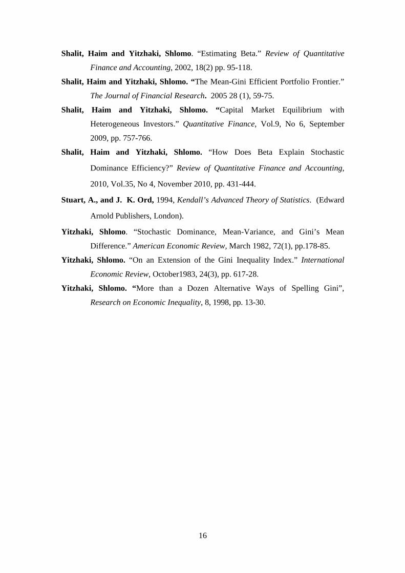
The first stage consists of constructing the MEG efficient frontier for a variety
of ν using the Excel routine. The efficient portfolios are calculated when short sales
are not allowed for ν = 2, 3, 4, 6, 8, 10, 15, 20, 40, 60, 80, 100. The results are shown
in Figure 2. In general, the various portfolio frontiers seem almost the same in shape,
concavity, and mean return corresponding to the minimum extended Gini. But still a
sizeable change in the trade-off between the mean return of the portfolio and the risk
expressed in (extended) Gini can be observed. A reduction of the mean return from
0.023 to 0.021 yields a risk improvement of 0.02 for ν = 2, but reduces risk by almost
0.1 for ν=100. Hence, the trade-off worsens considerably, reflecting the higher risk
aversion of the investor. The holdings of the minimum extended Gini portfolios are
presented in Table 2. The results display similar patterns with respect to the efficient
frontiers. Some sizable differences between the various portfolios can be observed:
the portfolios with higher risk aversion ν engage in stronger diversification and the
optimal portfolios with lower ν rely on a relative low number of assets.
The second stage of the optimization is performed by using the Mathematica
software. It generates efficient portfolios frontiers by varying the mean return, the
extended Gini, and the risk aversion parameter. The resulting 3-dimentional efficient
frontiers surfaces are displayed in Figure 4. In here, a rising risk aversion parameter
is accompanied by an increase in the risk compensation needed for a given reduction
in expected return. Furthermore, the figure illustrates that the speed of the trade-off
change does not follow a monotone pattern, but rather appears as a volatile process.
On the margin, it turns out that not even the change in the trade-off is a strictly
monotone function in the risk aversion parameter.

13
This rather unexpected result cannot only be explained by the non-continuous
adjustments in the optimal weights of the remaining assets whenever security is added
or removed from the optimal portfolio, but also from trade-offs inherent in the risk
aversion parameter itself. This argument can be explained using the elasticity of the
extended Gini with respect to the risk aversion parameter ν. From Equation (3) we
obtain the derivative of the extended Gini. Therefore, the elasticity w.r.t. ν is:
1
0
( ) 2 1ln(1 )
1x
x
dν ν ν
ν ϕ ϕν ν
∂Γ −= + −
∂ Γ − ∫ (9)
The ratio ( )2 1
1
νν−
− and the second term of Equation (9) create trade-offs that can lead
to non-monotony. In particular, this ratio exhibits singularity when ν → 1 or ν → 0
implying that near these values the extended Gini elasticity is non-monotonous. This
feature adds on top of the trade-off between risk bearing and diversification that can
raise the required mean returns.
5. Conclusions
We have presented a new approach to construct MEG portfolios by inserting the
coefficient of risk-aversion into the optimization program. Hence the results show a
three dimensional frontier where the risk-aversion coefficient can be chosen to
enhance the risk inherent in the portfolios. Not only the results deliver stochastic
dominant portfolios but they allow the analyst to offer a variety of alternatives for
risk-averse investors.
In addition, the paper provides some innovations of a more technical nature.
These include a Mathematica algorithm consisting of several interdependent
Mathematica packages and a notebook that allows for the efficient computation of
hulls by varying portfolios for a predefined set of assets. The size of this set is only
restricted by the computational resources available. In any case, these resources can
be improved by using the inherent parallel computing capacities of Mathematica. In
this way, the number of elements within the set of assets serving as the main input to
the algorithm can be almost unlimited.
It is exactly this computational power that allows also for a high degree of
flexibility in the design of the objective function within the process of the portfolio

14
optimization (5). Hence, future extensions of this research could include taking into
account higher moments and/or co-moments, additional parameters besides the risk-
aversion parameter and even a more general functional. Another potentially
interesting extension would be to include an objective function that not only reflects
the trade-off between return and risk, but also uses a measure of financial stability so
that minor shocks on the exogenous parameters and variables would not result in
major portfolio restructuring. Building on this argument, integrating transaction costs
into the objective function could potentially convey interesting results as well.

15
References
Bey, Roger P. and Howe, Keith M. “Gini's Mean Difference and Portfolio Selection:
An Empirical Evaluation.” Journal of Financial and Quantitative Analysis,
September 1984, 19(3), pp. 329-38.
Carroll, Carolyn, Thistle, Paul D. and Wei, John K. C. “The Robustness of Risk-
Return Nonlinearities to the Normality Assumption.” Journal of Financial
and Quantitative Analysis, September1992, 27(3), pp. 419-35.
Cheung, C. Sherman, Kwan, Clarence C. and Miu, Peter C.P. “Mean-Gini
Portfolio Analysis: A Pedagogic Illustration.” Spreadsheets in Education,
2005, 2(2), pp. 194-207
Fisher, Lawrence and Lorie, James H. “Some Studies of Variability of Returns on
Investments in Common Stocks.” Journal of Business, April 1970, 43(2), pp.
99-134.
Gastwirth, J. L ., “A General Definition of the Lorenz Curve.” Econometrica 39,
(1971), pp. 1037-1039.
Gregory-Allen, Russell B. and Shalit, Haim. “The Estimation of Systematic Risk
under Differentiated Risk Aversion: A Mean-Extended Gini Approach.”
Review of Quantitative Finance and Accounting, 1999, 12, pp. 135-57.
Lien, D. and Luo, X. “Estimating Extended Mean-Gini Coefficient for Futures
Hedging.” Journal of Futures Markets, 1993, 13, pp. 665-76
Okunev, John. “The Generation of Mean-Gini Efficient Sets.” Journal of Business,
Finance and Accounting, 1991, 18, pp. 209-18.
Shalit, Haim. ‘Mean-Gini Hedging in Futures Markets.” Journal of Futures Markets,
September 1995, 15(6) pp. 617-35.
Shalit, Haim and Yitzhaki, Shlomo. “Mean-Gini, Portfolio Theory and the Pricing
of Risky Assets.” Journal of Finance, December 1984, 39(5) pp.1449-68.
Shalit, Haim and Yitzhaki, Shlomo. “Evaluating the Mean-Gini Approach Selection
to Portfolio Selection.” International Journal of Finance, Spring 1989, 1(2)
pp. 15-31.
16
Shalit, Haim and Yitzhaki, Shlomo. “Estimating Beta.” Review of Quantitative
Finance and Accounting, 2002, 18(2) pp. 95-118.
Shalit, Haim and Yitzhaki, Shlomo. “The Mean-Gini Efficient Portfolio Frontier.”
The Journal of Financial Research. 2005 28 (1), 59-75.
Shalit, Haim and Yitzhaki, Shlomo. “Capital Market Equilibrium with
Heterogeneous Investors.” Quantitative Finance, Vol.9, No 6, September
2009, pp. 757-766.
Shalit, Haim and Yitzhaki, Shlomo. “How Does Beta Explain Stochastic
Dominance Efficiency?” Review of Quantitative Finance and Accounting,
2010, Vol.35, No 4, November 2010, pp. 431-444.
Stuart, A., and J. K. Ord, 1994, Kendall’s Advanced Theory of Statistics. (Edward
Arnold Publishers, London).
Yitzhaki, Shlomo. “Stochastic Dominance, Mean-Variance, and Gini’s Mean
Difference.” American Economic Review, March 1982, 72(1), pp.178-85.
Yitzhaki, Shlomo. “On an Extension of the Gini Inequality Index.” International
Economic Review, October1983, 24(3), pp. 617-28.
Yitzhaki, Shlomo. “More than a Dozen Alternative Ways of Spelling Gini”,
Research on Economic Inequality, 8, 1998, pp. 13-30.

17
Table 1: Summary Statistics for 100 stocks (Monthly Returns March 1992 – June 2007)
JB Stat Gini Std Dev Mean Firm JB Stat Gini Std Dev Mean Firm
6.76 6.14% 10.88% 1.64% HPQ 131.82 5.25% 9.30% 1.38% AA 36.34 3.64% 6.45% 0.78% IFF 6.26 3.36% 5.96% 1.09% ABT 15.33 5.15% 9.13% 1.40% IBM 8.67 8.32% 14.75% 2.31% AAPL 7.71 6.81% 12.07% 2.23% INTC 9.82 3.43% 6.07% 0.86% AEP
21.22 4.33% 7.68% 0.61% IP 263.03 9.23% 16.37% 2.21% AES 0.42 3.41% 6.05% 1.22% JNJ 22.71 3.64% 6.46% 1.37% AIG
32.40 5.05% 8.95% 1.50% JPM 55.14 5.59% 9.91% 1.56% AMGN 14.84 3.64% 6.45% 0.86% KO 292.58 5.20% 9.22% 1.75% AVP 11.00 5.55% 9.84% 1.21% LTD 49.9 3.88% 6.87% 1.66% AXP 10.67 3.85% 6.82% 1.23% MCD 37.76 4.41% 7.82% 1.26% BA 5.75 3.96% 7.02% 1.64% MDT 28.43 3.92% 6.95% 1.34% BAC
10.53 5.40% 9.57% 2.06% MER 73.44 4.24% 7.51% 1.20% BAX 29.54 3.35% 5.94% 1.15% MMM 5.47 5.54% 9.82% 1.58% BHI 35.37 4.70% 8.33% 1.46% MO 28.73 3.85% 6.82% 0.83% BMY 1.51 4.44% 7.86% 0.94% MRK 2.58 3.87% 6.87% 1.38% BNI
30.74 5.74% 10.18% 1.95% MSFT 0.23 2.74% 4.86% 1.02% BUD 1247.2 6.74% 11.94% 0.67% MAY 3.87 4.85% 8.60% 1.25% BDK 41.94 7.13% 12.63% 1.46% MEE 69.95 5.40% 9.57% 1.07% BC 13.19 4.51% 7.99% 1.18% NSC 4.74% 8.39% 2.06% C 8.23 9.21% 16.32% 2.27% NSM 31.22 4.72% 8.36% 1.92% CAT
953.11 11.03% 19.55% 1.30% NT 18.58 5.88% 10.42% 2.54% CCU 77.35 8.03% 14.23% 3.20% ORCL 222.53 5.03% 8.92% 1.83% CI 1.96 4.95% 8.77% 0.96% OMX 94.87 4.04% 7.15% 1.41% CL
14.84 4.32% 7.65% 1.58% OXY 7.51 5.30% 9.39% 1.66% CMCSA 74.30 3.48% 6.17% 1.10% PEP 8.4 3.86% 6.84% 1.51% COP 1.57 3.85% 6.82% 1.21% PFE 2.8 3.69% 6.54% 0.97% CPB
389.57 3.48% 6.17% 1.22% PG 134.2 5.68% 10.07% 1.41% CSC 9.66 3.23% 5.72% 0.91% RF 5.12 6.83% 12.11% 2.89% CSCO
83.38 5.24% 9.30% 2.36% ROK 28.54 4.42% 7.84% 1.30% CVS 162.61 4.78% 8.48% 0.92% RTN 14.86 3.14% 5.56% 1.35% CVX
0.98 6.42% 11.38% 1.56% RSH 5.47 4.94% 8.76% 1.52% CEN 65.71 5.31% 9.42% 1.33% S 0.51 3.79% 6.71% 0.89% DD 37.35 3.98% 7.05% 0.74% SLB 5.98 8.34% 14.79% 3.42% DELL 27.79 3.06% 5.42% 1.58% SO 13.08 4.23% 7.50% 0.89% DIS 11.74 4.12% 7.31% 1.12% T 131.58 4.28% 7.59% 1.03% DOW 54.91 7.16% 12.69% 1.91% TEK 42.66 4.77% 8.45% 0.57% EK 2.58 4.48% 7.93% 1.79% TGT 1.83 8.35% 14.79% 3.40% EMC
88.95 9.07% 16.08% 4.03% TWX 150.36 6.18% 10.96% 1.28% EP 10.17 7.27% 12.89% 2.50% TXN 23.56 3.62% 6.42% 1.65% ETR
207.48 5.56% 9.86% 1.66% TYC 50.88 3.86% 6.85% 1.55% EXC 131.57 4.19% 7.43% 1.42% USB 20.96 5.39% 9.56% 0.86% F 125.09 3.97% 7.04% 1.73% UTX 21.41 4.77% 8.45% 1.59% FDX 152.00 4.11% 7.29% 0.98% VZ 1951.85 5.14% 9.10% 2.70% GD 47.55 4.08% 7.24% 0.94% WB 3.49 3.43% 6.08% 1.36% GE 19.20 3.72% 6.59% 1.56% WFC 0.49 5.42% 9.61% 0.88% GM
267.65 7.34% 13.01% 2.18% WMB 9.69 6.19% 10.97% 1.87% HAL 4.43 4.03% 7.14% 1.02% WMT 4.13 4.55% 8.07% 1.30% HD 0.49 4.18% 7.41% 1.14% WY 112.68 6.06% 10.74% 2.25% HET
505.79 7.21% 12.79% 1.18% XRX 0.79 3.15% 5.58% 0.93% HNZ 56.74 2.68% 4.74% 1.35% XOM 339.23 5.17% 9.16% 1.40% HON

18
Table 2: Holdings of Minimum Extended Gini Portfolios for various ν, showing only the non-zero positions
Firms ν=2 ν=3 ν=4 ν=6 ν=8 ν=10 ν=15 ν=20 ν=40 ν=60 ν=80 ν=100
ABT 2.99% 4.69% 5.48% 5.58% 5.64% 5.28% 5.14% 4.63% 5.07% 5.07% 5.07% 5.07%
AAPL 0.23% 0.61% 1.01% 2.10% 3.39% 4.84% 5.49% 6.00% 7.11% 7.12% 7.12% 7.12%
AMGN 1.40% 1.21% 0.97% 0.82% 0.75% 2.60% 2.53% 2.94% 2.16% 2.16% 2.16% 2.16%
BNI 1.68% 1.76% 1.72% 1.51% 1.22% 0.10% 0.10% 0.09% 0.08% 0.08% 0.08% 0.08%
BUD 17.50% 15.20% 13.85% 12.24% 11.55% 11.79% 11.71% 11.24% 13.16% 13.18% 13.18% 13.18%
COP 0.00% 0.00% 0.09% 0.09% 0.09% 0.13% 0.14% 0.14% 0.13% 0.13% 0.13% 0.13%
CPB 0.00% 0.00% 0.00% 0.01% 0.01% 0.01% 0.01% 0.01% 0.01% 0.01% 0.01% 0.01%
CVX 8.91% 8.38% 7.21% 5.72% 4.87% 4.26% 3.68% 2.15% 0.69% 0.69% 0.69% 0.69%
CEN 0.00% 0.00% 0.00% 0.00% 0.00% 0.00% 0.00% 0.00% 0.50% 0.50% 0.50% 0.50%
DOW 2.22% 2.55% 2.44% 2.25% 2.65% 3.87% 3.61% 2.51% 1.25% 1.25% 1.25% 1.25%
EK 2.96% 3.63% 3.76% 4.15% 4.38% 3.39% 3.57% 4.03% 5.05% 5.06% 5.06% 5.06%
EXC 5.29% 4.34% 3.84% 3.46% 3.50% 3.13% 1.84% 1.18% 1.19% 1.19% 1.19% 1.19%
FDX 0.70% 0.76% 0.79% 0.78% 0.69% 0.34% 0.33% 0.32% 0.31% 0.31% 0.31% 0.31%
GD 2.02% 1.18% 0.78% 0.51% 0.46% 0.84% 1.12% 2.74% 7.05% 7.05% 7.05% 7.05%
HET 0.35% 0.00% 0.00% 0.00% 0.00% 0.00% 0.00% 0.20% 0.20% 0.20% 0.20% 0.20%
HNZ 8.00% 8.10% 8.47% 7.82% 8.16% 8.05% 8.54% 8.08% 4.02% 4.02% 4.02% 4.02%
LTD 0.00% 0.63% 0.74% 0.91% 1.16% 3.87% 4.17% 5.06% 5.42% 5.41% 5.41% 5.41%
MDT 2.01% 2.26% 2.25% 1.72% 1.34% 0.00% 0.00% 0.00% 0.60% 0.60% 0.60% 0.60%
MER 0.00% 0.00% 0.00% 0.00% 0.00% 0.00% 0.00% 0.00% 0.06% 0.06% 0.06% 0.06%
MMM 4.27% 3.65% 2.71% 2.12% 1.80% 0.21% 0.20% 0.16% 0.14% 0.14% 0.14% 0.14%
MO 0.00% 0.00% 0.00% 0.00% 0.00% 0.00% 0.00% 0.14% 0.11% 0.11% 0.11% 0.11%
MSFT 3.61% 2.61% 2.39% 2.42% 2.22% 1.69% 1.33% 1.10% 0.59% 0.59% 0.59% 0.59%
NSM 1.05% 0.87% 0.87% 0.91% 0.70% 0.14% 0.15% 0.11% 0.09% 0.09% 0.09% 0.09%
ORCL 1.53% 2.27% 2.59% 3.60% 3.69% 4.12% 3.92% 3.55% 3.91% 3.90% 3.90% 3.90%
PG 0.15% 0.11% 0.10% 0.10% 0.10% 0.17% 0.18% 0.13% 0.11% 0.11% 0.11% 0.11%
RSH 3.62% 4.31% 4.40% 3.91% 3.26% 2.08% 1.36% 0.65% 0.28% 0.28% 0.28% 0.28%
S 0.00% 0.68% 0.86% 0.91% 0.91% 0.45% 0.44% 0.40% 0.30% 0.30% 0.30% 0.30%
SLB 0.00% 0.00% 0.00% 0.04% 0.04% 0.04% 0.04% 0.05% 0.05% 0.05% 0.05% 0.05%
SLE 0.00% 0.00% 0.00% 0.84% 0.88% 1.44% 1.66% 1.77% 1.57% 1.57% 1.57% 1.57%
SO 19.66% 23.58% 25.70% 28.02% 29.11% 31.13% 32.48% 33.32% 31.94% 31.86% 31.86% 31.86%
T 0.00% 0.00% 0.00% 1.27% 1.44% 2.79% 2.82% 2.78% 0.70% 0.70% 0.70% 0.70%
TEK 2.75% 2.44% 2.60% 2.91% 3.12% 3.11% 3.31% 4.32% 5.74% 5.73% 5.73% 5.73%
Total 92.91% 95.80% 95.62% 96.73% 97.13% 99.88% 99.88% 99.81% 99.61% 99.54% 99.54% 99.54%

19
Figure 1: The Absolute Lorenz Curve
0 1
E(X)
φ
LSA
Lφ)
α
L(α)

20
Figure 2: Efficient Frontiers for Various νs
Efficient frontier Mean-Gini (nu=2)
0.005
0.007
0.009
0.011
0.013
0.015
0.017
0.019
0.021
0.023
0.025
0.013 0.015 0.017 0.019 0.021 0.023
Gini
Mea
n
Efficient Frontier Mean Extended Gini(Nu=3)
0.005
0.007
0.009
0.011
0.013
0.015
0.017
0.019
0.021
0.023
0.025
0.02 0.022 0.024 0.026 0.028 0.03 0.032
Extended Gini(nu=3)
Mea
n
Efficient Frontier Mean Extended Gini( nu=4)
0.005
0.007
0.009
0.011
0.013
0.015
0.017
0.019
0.021
0.023
0.025
0.02 0.025 0.03 0.035 0.04
Extended Gini(nu=4)
Mea
n
Efficient Fontier Mean Extended Gini(nu= 6)
0.005
0.007
0.009
0.011
0.013
0.015
0.017
0.019
0.021
0.023
0.025
0.02 0.025 0.03 0.035 0.04 0.045 0.05
Extended Gini(nu=6)
Mea
n
Efficient Frontier Mean Extended Gini(nu=8)
0.005
0.007
0.009
0.011
0.013
0.015
0.017
0.019
0.021
0.023
0.025
0.02 0.025 0.03 0.035 0.04 0.045 0.05 0.055
Extended Gini(nu=8)
Mea
n
Efficient Frontier Mean Extended Gini(nu= 10)
0.005
0.007
0.009
0.011
0.013
0.015
0.017
0.019
0.021
0.023
0.025
0.02 0.025 0.03 0.035 0.04 0.045 0.05 0.055 0.06
Extended Gini(nu=10)
Mea
n
21
Figure 2: cont.
Efficient Frontier Mean Extended Gini(nu=15)
0.005
0.007
0.009
0.011
0.013
0.015
0.017
0.019
0.021
0.023
0.025
0.02 0.03 0.04 0.05 0.06 0.07
Extended Gini(nu=15)
Mea
n
Efficient Frontier Mean Extended Gini(20)
0.005
0.007
0.009
0.011
0.013
0.015
0.017
0.019
0.021
0.023
0.025
0.02 0.03 0.04 0.05 0.06 0.07 0.08
Extended Gini(nu=20)
Mea
n
Efficient Frontier Mean Extended Gini(40)
0.005
0.007
0.009
0.011
0.013
0.015
0.017
0.019
0.021
0.023
0.025
0.02 0.03 0.04 0.05 0.06 0.07 0.08
Extended Gini(nu=40)
Mea
n
Efficient Frontier Mean Extended Gini(60)
0.005
0.007
0.009
0.011
0.013
0.015
0.017
0.019
0.021
0.023
0.025
0.02 0.03 0.04 0.05 0.06 0.07 0.08
Extended Gini(nu=60)
Mea
n
Efficient Frontier Mean Extended Gini(80)
0.005
0.007
0.009
0.011
0.013
0.015
0.017
0.019
0.021
0.023
0.025
0.02 0.03 0.04 0.05 0.06 0.07 0.08
Extended Gini(nu=80)
Mea
n
Efficient Frontier Mean Extended Gini(100)
0.005
0.007
0.009
0.011
0.013
0.015
0.017
0.019
0.021
0.023
0.025
0.02 0.03 0.04 0.05 0.06 0.07 0.08
Extended Gini(nu=100)
Mea
n

22
Figure 3: Flowchart for Mathematica Package

23
Figure 4: 3-D Efficiency Frontier Mean Extended Gini
Mean-extendedGini-Risk ParameterEfficient Portfolio Frontier
-0.05
0.
Mean
26
1014
18
22
26
30
34
38
Risk param
0 0.02 0.04 0.06 0.08
Extended Gini
![Gini Coefficient California pre-tax income, 2000, Gini=62.1%saez/course131/taxintro_ch17_new_attach.pdfFigure 1: Gini coefficient 6RXUFH .RSF]XN 6DH] 6RQJ4-( :DJHHDUQLQJVLQHTXDOLW\](https://static.fdocuments.net/doc/165x107/5f9d687763df8333422405c5/gini-coefficient-california-pre-tax-income-2000-gini621-saezcourse131taxintroch17newattachpdf.jpg)


![Issues in Optimization of Decision Tree Learning: A Survey · 2013. 1. 9. · gini T gini T gini T NN (8) Breiman et al. [9] identified that the gini index has a problem criterion](https://static.fdocuments.net/doc/165x107/61103ba40a374f30f33eb7c7/issues-in-optimization-of-decision-tree-learning-a-survey-2013-1-9-gini-t.jpg)