MCQMC 2016 Tutorial
56
Error Analysis for Quasi-Monte Carlo Methods Fred J. Hickernell Department of Applied Mathematics, Illinois Institute of Technology [email protected] mypages.iit.edu/~hickernell Thanks to the Guaranteed Automatic Integration Library (GAIL) team and friends Supported by NSF-DMS-1522687 Thanks to the MCQMC 2016 organizers
-
Upload
fred-j-hickernell -
Category
Science
-
view
63 -
download
0
Transcript of MCQMC 2016 Tutorial

Error Analysis for Quasi-Monte Carlo Methods
Fred J. HickernellDepartment of Applied Mathematics, Illinois Institute of Technology
[email protected] mypages.iit.edu/~hickernell
Thanks to the Guaranteed Automatic Integration Library (GAIL) team and friends
Supported by NSF-DMS-1522687
Thanks to the MCQMC 2016 organizers

Introduction Trio Error Identity Tractability Rewriting the Problem When to Stop References
August 12, 2016 News
Can a more clever brute-forcing give us a better picture?
2/38

Introduction Trio Error Identity Tractability Rewriting the Problem When to Stop References
Error Analysis for Quasi-Monte Carlo Methods
µ := E[f (X)] :=ż
X
f (x)ν(dx) « µ̂ :=nÿ
i=1f (xi)wi =
ż
X
f (x) ν̂(dx)
µ´ µ̂ =
ż
X
f (x) (ν´ ν̂)(dx) = ?
Reality Error Analysis (Theory)What is What we think it should be
by rigorous argumentNot certain that
our assumptions hold
Quasi-Monte Carlo Methodsw1 = ¨ ¨ ¨ = wn = 1/n orxi chosen carefully
3/38

Introduction Trio Error Identity Tractability Rewriting the Problem When to Stop References
Integration Examplesµ =
1N
Nÿ
j=1f (j) = population average hours of sleep
f (j) = hours of sleep for individual j
µ =
ż
Rdf (x)ν(dx) = option price
f (x) = discounted payoff determined by market forces x
µ =
ż
X
g(x)dx = P(X P X) = probability
g = probability density function
µ = E[f (X)] =ż
X
f (x)ν(dx) « µ̂ =nÿ
i=1f (xi)wi =
ż
X
f (x) ν̂(dx) µ´ µ̂ = ?
ν = probability measure, ν̂ =nÿ
i=1wiδxi = sampling measure
4/38

Introduction Trio Error Identity Tractability Rewriting the Problem When to Stop References
Trio Identity for the Error (Meng, 2016+)
µ´ µ̂ =
ż
X
f (x)ν(dx)´nÿ
i=1f (xi)wi =
ż
X
f (x) (ν´ ν̂)(dx)
= ALN(f , ν´ ν̂) DSC(ν´ ν̂) VAR(f )
VAR(f ) = variation of the integrand ě 0DSC(ν´ ν̂) = discrepancy of the sampling measure
from the probability measure ě 0expect this to track error as n Ñ∞
ALN(f , ν´ ν̂) = alignment between the integrand andthe difference between the two measures
should not be ignored
Sampling Measure, ν̂Integrand, f Fixed Random
Fixed Deterministic = D Randomized = R
Gaussian Process Bayesian = B Bayesian Randomized = BR5/38

Introduction Trio Error Identity Tractability Rewriting the Problem When to Stop References
Deterministic Trio Identity(F, ‖¨‖F) = normed vector space of integrands
f ÞÑ f (x) is bounded for all x P X(M, ‖¨‖M) = normed vector space of signed measures
‖λ‖M := sup0‰fPF
∣∣şX
f (x) λ(dx)∣∣
‖f‖F
µ´ µ̂ =
ż
X
f (x) (ν´ ν̂)(dx)
=
ş
Xf (x) (ν´ ν̂)(dx)‖ν´ ν̂‖M ‖f‖F
looooooooooomooooooooooon
ALND(f , ν´ ν̂)
‖ν´ ν̂‖Mloooomoooon
DSCD(ν´ ν̂)
‖f‖Floomoon
VARD(f )
∣∣ALND(f , ν´ ν̂)∣∣ ď 1
Ignoring ALND(f , ν´ ν̂) yields a generalized Koksma-Hlawka inequality(Hlawka, 1961; Niederreiter, 1992; H., 1998; 1999)
.6/38

Introduction Trio Error Identity Tractability Rewriting the Problem When to Stop References
Hours of Sleep Web Surveyµ = population average hours of sleep
f (j) = hours of sleep for individual jν = uniform on t1, . . . ,Nu
ν̂ = uniform on a set of distinct individuals, txiuni=1
µ = µ(f ) = population mean cov(f , g) = population covariance
=1N
Nÿ
j=1f (j) =
1N
Nÿ
i=1[f (j)´ µ(f )][g(j)´ µ(g)]
µ´ µ̂ = ´ corr(f ,1txiu
ni=1
)loooooooooomoooooooooon
ALND(f , ν´ ν̂)
d
1´ n/Nn/N
looooomooooon
DSCD(ν´ ν̂)
std(f )loomoon
VARD(f )
Discrepancy depends on the sample fraction, not merely the sample size(Meng, 2016+)Correlation for a web survey is difficult to control or predict
7/38

Introduction Trio Error Identity Tractability Rewriting the Problem When to Stop References
Reproducing Kernel Hilbert Spaces (RKHS)If F is a Hilbert space of integrands with reproducing kernel K : Xˆ XÑ R, thenthe cubature error is the inner product of the integrand with the representer for theerror functional (H., 1999):
VAR(f ) = ‖f‖F , f (t) = xK(¨, t), f yF @t P X, f P F
[DSC(ν´ ν̂)]2 =
ż
X2K(x, t)ν(dx)ν(dt)´ 2
nÿ
i=1wi
ż
X
K(xi, t)ν(dt)
+nÿ
i,j=1wiwjK(xi, xj) = k0 ´ 2kTw+wTKw
ALN(f , ν´ ν̂) = cos(
f ,ż
X
K(¨, t)ν(dt)´nÿ
j=1wjK(¨, xj)
looooooooooooooooooomooooooooooooooooooon
cubature error representer
),
cos(f , g) :=xf , gyF
‖f‖F ‖g‖F
µ´ µ̂ = cos(f , error rep)DSCD(ν´ ν̂) ‖f‖F8/38

Introduction Trio Error Identity Tractability Rewriting the Problem When to Stop References
L2-Discrepancyν = uniform on X = [0, 1]d, ν̂ = uniform on txiu
ni=1
K(x, t) =dź
k=1[2´max(xk, tk)] (H., 1998)
VARD(f ) = ‖f ´ f (1)‖F =∥∥∥(‖Buf‖L2
)H‰uĎ1:d
∥∥∥2, Buf := B|u|f
Bxu
∣∣∣∣xsu = 1
[DSCD(ν´ ν̂)]2 =
(43
)d´
2n
nÿ
i=1
dź
k=1
(3´ x2
ik2
)+
1n2
nÿ
i,j=1
dź
k=1[2´max(xik, xjk)]
9/38

Introduction Trio Error Identity Tractability Rewriting the Problem When to Stop References
L2-Discrepancyν = uniform on X = [0, 1]d, ν̂ = uniform on txiu
ni=1
K(x, t) =dź
k=1[2´max(xk, tk)] (H., 1998)
VARD(f ) = ‖f ´ f (1)‖F =∥∥∥(‖Buf‖L2
)H‰uĎ1:d
∥∥∥2, Buf := B|u|f
Bxu
∣∣∣∣xsu = 1
[DSCD(ν´ ν̂)]2 =
(43
)d´
2n
nÿ
i=1
dź
k=1
(3´ x2
ik2
)+
1n2
nÿ
i,j=1
dź
k=1[2´max(xik, xjk)]
=∥∥∥(‖ν([0, ¨u])´ ν̂([0, ¨u])‖L2
)H‰uĎ1:d
∥∥∥2geometric interpretation
x = (. . . , 0.6, . . . , 0.4, . . .)
ν([0, xt5,8u])´ ν̂([0, xt5,8u])
= 0.24´ 7/32 = 0.02125
9/38

Introduction Trio Error Identity Tractability Rewriting the Problem When to Stop References
L2-Discrepancyν = uniform on X = [0, 1]d, ν̂ = uniform on txiu
ni=1
K(x, t) =dź
k=1[2´max(xk, tk)] (H., 1998)
VARD(f ) = ‖f ´ f (1)‖F =∥∥∥(‖Buf‖L2
)H‰uĎ1:d
∥∥∥2, Buf := B|u|f
Bxu
∣∣∣∣xsu = 1
[DSCD(ν´ ν̂)]2 =
(43
)d´
2n
nÿ
i=1
dź
k=1
(3´ x2
ik2
)+
1n2
nÿ
i,j=1
dź
k=1[2´max(xik, xjk)]
=∥∥∥(‖ν([0, ¨u])´ ν̂([0, ¨u])‖L2
)H‰uĎ1:d
∥∥∥2geometric interpretation
µ´ µ̂ = cos(f , error rep)DSCD(ν´ ν̂) ‖f ´ f (1)‖FDSCD(ν´ ν̂) requires O(dn2) operations to evaluate
DSCD(ν´ ν̂)
$
’
’
’
’
’
’
’
&
’
’
’
’
’
’
’
%
= O(n´1/2) on average for IID Monte Carlo= O(n´1+ε) for digital nets, integration lattices, . . .
(Niederreiter, 1992; Dick and Pillichshammer, 2010)ě O(n´1) for all ν̂ because this K has limited smoothness= O(n´r) for r ą 1 for smoother K and higher order nets
(Dick, 2008) 9/38
Introduction Trio Error Identity Tractability Rewriting the Problem When to Stop References
Multivariate Normal Probabilityµ =
ż
[a,b]
exp(´ 1
2tTΣ´1t
)a
(2π)d det(Σ)dt Genz (1993)
=
ż
[0,1]d´1f (x)dx
ν̂ = uniform on txiuni=1
µ´ µ̂ = cos(f , error rep)DSCD(ν´ ν̂) ‖f ´ f (1)‖F
DSCD(ν´ ν̂)#
= O(n´1/2) for IID MC= O(n´1+ε) for Sobol’
10/38

Introduction Trio Error Identity Tractability Rewriting the Problem When to Stop References
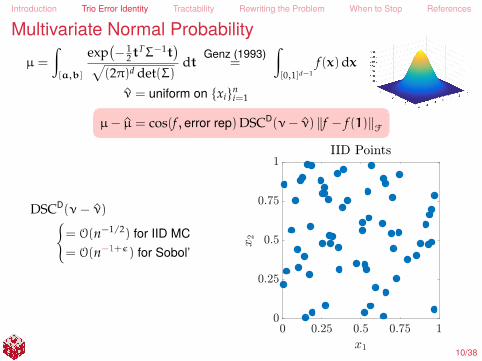
Multivariate Normal Probabilityµ =
ż
[a,b]
exp(´ 1
2tTΣ´1t
)a
(2π)d det(Σ)dt Genz (1993)
=
ż
[0,1]d´1f (x)dx
ν̂ = uniform on txiuni=1
µ´ µ̂ = cos(f , error rep)DSCD(ν´ ν̂) ‖f ´ f (1)‖F
DSCD(ν´ ν̂)#
= O(n´1/2) for IID MC= O(n´1+ε) for Sobol’
For some typical choice ofa, b, Σ, and d = 3
µ « 0.6763
+
Low discrepancy samplingreduces cubature error
10/38

Introduction Trio Error Identity Tractability Rewriting the Problem When to Stop References
Randomized Trio Identity
ν̂ = random measure with probability Pν̂(F, ‖¨‖F) as before, but f ÞÑ f (x) need not be bounded
µ´ µ̂ =
ş
Xf (x) (ν´ ν̂)(dx)
DSC(ν´ ν̂)VAR(f )loooooooooooomoooooooooooon
ALNR(f , ν´ ν̂)
sup0‰fPF
d
Eν̂[ş
Xf (x) (ν´ ν̂)(dx)
]2
‖f‖Flooooooooooooooooooooomooooooooooooooooooooon
DSCR(ν´ ν̂)
‖f‖Floomoon
VARD(f )
E∣∣ALNR(f , ν´ ν̂)
∣∣2 ď 1
DSCR(ν´ ν̂) ď
b
E∣∣DSCD(ν´ ν̂)
∣∣2
11/38

Introduction Trio Error Identity Tractability Rewriting the Problem When to Stop References
IID Monte Carlo
If ν̂ is an equally weighted average of n integrand values at IID data sites, then
std(f ) := ‖f ´ µ‖L2 :=
d
ż
X
|f (x)´ µ|2 ν(dx)
µ´ µ̂ =
?nş
Xf (x) (ν´ ν̂)(dx)
std(f )loooooooooooooomoooooooooooooon
ALNR(f , ν´ ν̂)
1?
nloomoon
DSCR(ν´ ν̂)
std(f )loomoon
VARD(f )
ALNR(f , ν´ ν̂) „ (0, 1), µ̂ is unbiased« N(0, 1) for large n by the Central Limit Theorem
12/38

Introduction Trio Error Identity Tractability Rewriting the Problem When to Stop References
Hours of Sleep Simple Random Survey w/o Replacementµ = population average hours of sleep
f (j) = hours of sleep for individual jsimple random sampling, txiu
ni=1, w/o replacement
µ´ µ̂ =
$
’
’
’
’
&
’
’
’
’
%
´ corr(f ,1txiu
ni=1
) d
1´ n/Nn/N
std(f ) web
´ corr(f ,1txiu
ni=1
)stdν̂
(corr
(f ,1txiu
ni=1
))d 1´ n/Nn(1´ 1/N)
std(f ) simple random
The vast majority of designs, txiuni=1, have corr
(f ,1txiu
ni=1
)= O(1/
?N), but
your web survey is likely one of the awful minority that does notThe error of a web survey with nweb samples is equivalent to the error of
survey with nSRS «nweb/N
corr2(f ,1txiu
ni=1
)(1´ nweb/N)
simple random samples
nweb = 1 million distinct samples from a population of N = 250 million with acorrelation of 0.05 is about as valuable as nSRS = 1.6 simple randomsamples
13/38

Introduction Trio Error Identity Tractability Rewriting the Problem When to Stop References
Multivariate Normal Probabilityµ =
ż
[a,b]
exp(´ 1
2tTΣ´1t
)a
(2π)d det(Σ)dt Genz (1993)
=
ż
[0,1]d´1f (x)dx
µ´ µ̂ =
"
cos(f , error rep) DSCD(ν´ ν̂)
ALNR(f , ν´ ν̂) DSCR(ν´ ν̂)
*
VARD(f )
For scrambled Sobol’ pointsDSCD(ν´ ν̂) = O(n´1+ε)
DSCR(ν´ ν̂) = O(n´3/2+ε)
(Owen, 1997; H. and Yue, 2000;Heinrich et al., 2004)
14/38

Introduction Trio Error Identity Tractability Rewriting the Problem When to Stop References
Multivariate Normal Probabilityµ =
ż
[a,b]
exp(´ 1
2tTΣ´1t
)a
(2π)d det(Σ)dt Genz (1993)
=
ż
[0,1]d´1f (x)dx
µ´ µ̂ =
"
cos(f , error rep) DSCD(ν´ ν̂)
ALNR(f , ν´ ν̂) DSCR(ν´ ν̂)
*
VARD(f )
For scrambled Sobol’ pointsDSCD(ν´ ν̂) = O(n´1+ε)
DSCR(ν´ ν̂) = O(n´3/2+ε)
(Owen, 1997; H. and Yue, 2000;Heinrich et al., 2004)
For some typical choice ofa, b, Σ, and d = 3
µ « 0.6763
+
Randomized sampling, ν̂, mayavoid the awful minority
14/38

Introduction Trio Error Identity Tractability Rewriting the Problem When to Stop References
Pricing an Asian Option
µ =
ż
Rdpayoff(t)
exp(´ 1
2tTΣ´1t
)a
(2π)d det(Σ)dt =
ż
[0,1]df (x)dx
µ´ µ̂ =
"
cos(f , error rep) DSCD(ν´ ν̂)
ALNR(f , ν´ ν̂) DSCR(ν´ ν̂)
*
VARD(f )
For an Asian arithmetic meanoption, d = 12, µ « $13.1220
*
Scrambled Sobol’ does notachieve O(n´3/2+ε) conver-gence because f is not smoothenough.
f is not even smooth enoughfor O(n´1+ε) convergence, ex-cept by a delicate argument(Griebel et al., 2010; 2016+)
15/38

Introduction Trio Error Identity Tractability Rewriting the Problem When to Stop References
Summary So Far
µ´ µ̂ = ?
Reality Error Analysis (Theory)What is What we think it should be
Trio identity: µ´ µ̂ = ALN(f , ν´ ν̂) DSC(ν´ ν̂) VAR(f ) —keep all
termsBig data may not eliminate the need for proper sampling—simple randomsampling beats haphazard samplingLow discrepancy sampling beats simple random samplingRandomization to remove bias can improve convergence rate
16/38

Introduction Trio Error Identity Tractability Rewriting the Problem When to Stop References
Bayesian Trio IdentityRandom f postulated by Diaconis (1988), O’Hagan (1991), Ritter (2000),Rasmussen and Ghahramani (2003) and others: f „ GP(0, s2Cθ), a Gaussianprocess from the sample space F with zero mean and covariance kernel, s2Cθ,Cθ : Xˆ XÑ R. The scale parameter, s, and shape parameter, θ, should beestimated. Then
c0 =
ż
X2C(x, t)ν(dx)ν(dt), c =
(ż
X
C(xi, t)ν(dt))n
i=1
C =(C(xi, xj)
)ni,j=1, w =
(wi)n
i=1
µ´ µ̂ =
ş
Xf (x) (ν´ ν̂)(dx)
sa
c0 ´ 2cTw+wTCwloooooooooooooomoooooooooooooon
ALNB(f , ν´ ν̂)
a
c0 ´ 2cTw+wTCwlooooooooooooomooooooooooooon
DSCB(ν´ ν̂)
sloomoon
VARB(f )
w = C´1c minimizes DSCB(ν´ ν̂)makes ALNB(f , ν´ ν̂)
ˇ
ˇtf (xi) = yiuni=1 „ N(0, 1)
DSCB(ν´ ν̂) = DSCD(ν´ ν̂) if Cθ = K
17/38

Introduction Trio Error Identity Tractability Rewriting the Problem When to Stop References
Bayesian Cubature
Deterministic Interpretation
f „ GP(0, s2Cθ) f P F w/ reproducing kernel Kθ∣∣ALNB∣∣DSCB(ν´ ν̂)VARB(f ) = |µ´ µ̂| =∣∣ALND∣∣DSCD(ν´ ν̂)VARD()
with 99% confidence ď width if VARD(f ´rfy) ď2.58?
nVARD(rfy)
2.58
d(cθ̂,0 ´ cT
θ̂C´1θ̂cθ̂) yTC´1
θ̂y
nÐwidthÑ replace Cθ by Kθ
= 2.58 DSCB(ν´ ν̂)VARB(f ) =2.58?
nDSCD(ν´ ν̂)VARD(rfy)
y =(f (xi)
)ni=1
rfy = minimum norm interpolantC´1θ̂cθ̂ Ð wÑ replace Cθ by Kθ
argminθ
yTC´1θ y
[det(C´1θ )]1/n
Ð θ̂Ñ replace Cθ by Kθ
estimate s and θ by MLE = argminθ
vol( z P Rn :
VARDθ(rfz) ď VARD
θ(rfy)
()Nice:
y, Cθ w µ̂ width θ̂
47y, 29Cθ w 47µ̂ 47width θ̂ 18/38

Introduction Trio Error Identity Tractability Rewriting the Problem When to Stop References
Multivariate Normal Probabilityµ =
ż
[a,b]
exp(´ 1
2tTΣ´1t
)a
(2π)d det(Σ)dt Genz (1993)
=
ż
[0,1]d´1f (x)dx
µ´ µ̂ =
$
&
%
cos(f , error rep) DSCD(ν´ ν̂) VARD(f )ALNR(f , ν´ ν̂) DSCR(ν´ ν̂) VARD(f )
ALNB(f , ν´ ν̂) DSCB(ν´ ν̂) VARB(f )
,
.
-
Use a product Matérn kernelwith modest smoothness:
Cθ(x, t)
=dź
k=1(1+θ |xk ´ tk|)e´θ|xk´tk|
19/38

Introduction Trio Error Identity Tractability Rewriting the Problem When to Stop References
Multivariate Normal Probabilityµ =
ż
[a,b]
exp(´ 1
2tTΣ´1t
)a
(2π)d det(Σ)dt Genz (1993)
=
ż
[0,1]d´1f (x)dx
µ´ µ̂ =
$
&
%
cos(f , error rep) DSCD(ν´ ν̂) VARD(f )ALNR(f , ν´ ν̂) DSCR(ν´ ν̂) VARD(f )ALNB(f , ν´ ν̂) DSCB(ν´ ν̂) VARB(f )
,
.
-
Smaller error using Bayesiancubature with scrambled
Sobol’ data sitesRequires O(n3)operations to computeC´1θ , but see Anitescu et al.
(2016)Ill-conditioning forsmoother kernels (fasterconvergence)
19/38

Introduction Trio Error Identity Tractability Rewriting the Problem When to Stop References
Multivariate Normal Probabilityµ =
ż
[a,b]
exp(´ 1
2tTΣ´1t
)a
(2π)d det(Σ)dt Genz (1993)
=
ż
[0,1]d´1f (x)dx
µ´ µ̂ =
$
&
%
cos(f , error rep) DSCD(ν´ ν̂) VARD(f )ALNR(f , ν´ ν̂) DSCR(ν´ ν̂) VARD(f )ALNB(f , ν´ ν̂) DSCB(ν´ ν̂) VARB(f )
,
.
-
Confidence intervals succeed« 98% of the time
19/38

Introduction Trio Error Identity Tractability Rewriting the Problem When to Stop References
Bayesian Cubature Deterministic Interpretationf „ GP(0, s2Cθ) f P F w/ reproducing kernel Kθ∣∣ALNB∣∣DSCB(ν´ ν̂)VARB(f ) = |µ´ µ̂| =
∣∣ALND∣∣DSCD(ν´ ν̂)VARD(f )
with 99% confidence ď width if VARD(f ´rfy) ď2.58?
nVARD(rfy)
2.58
d(cθ̂,0 ´ cT
θ̂C´1θ̂cθ̂) yTC´1
θ̂y
nÐwidthÑ replace Cθ by Kθ
= 2.58 DSCB(ν´ ν̂)VARB(f ) =2.58?
nDSCD(ν´ ν̂)VARD(rfy)
y =(f (xi)
)ni=1
rfy = minimum norm interpolantC´1θ̂cθ̂ Ð wÑ replace Cθ by Kθ
argminθ
yTC´1θ y
[det(C´1θ )]1/n
Ð θ̂Ñ replace Cθ by Kθ
estimate s and θ by MLE = argminθ
vol( z P Rn :
VARDθ(rfz) ď VARD
θ(rfy)
()20/38

Introduction Trio Error Identity Tractability Rewriting the Problem When to Stop References
Bayesian Cubature Deterministic Interpretationf „ GP(0, s2Cθ) f P F w/ reproducing kernel Kθ∣∣ALNB∣∣DSCB(ν´ ν̂)VARB(f ) = |µ´ µ̂| =
∣∣ALND∣∣DSCD(ν´ ν̂)VARD(f ´rfy)
with 99% confidence ď width if VARD(f ´rfy) ď2.58?
nVARD(rfy)
2.58
d(cθ̂,0 ´ cT
θ̂C´1θ̂cθ̂) yTC´1
θ̂y
nÐwidthÑ replace Cθ by Kθ
= 2.58 DSCB(ν´ ν̂)VARB(f ) =2.58?
nDSCD(ν´ ν̂)VARD(rfy)
y =(f (xi)
)ni=1
rfy = minimum norm interpolantC´1θ̂cθ̂ Ð wÑ replace Cθ by Kθ
argminθ
yTC´1θ y
[det(C´1θ )]1/n
Ð θ̂Ñ replace Cθ by Kθ
estimate s and θ by MLE = argminθ
vol( z P Rn :
VARDθ(rfz) ď VARD
θ(rfy)
()Requires O(n3) operations to compute C´1
θ , but see Anitescu et al. (2016)Ill-conditioning for smoother kernels (faster convergence)
20/38

Introduction Trio Error Identity Tractability Rewriting the Problem When to Stop References
Randomized Bayesian Trio Identityf „ GP(0, s2C) and ν̂ is random (independent of f ):
µ´ µ̂ =
ş
Xf (x) (ν´ ν̂)(dx)
sb
Eν̂(c0 ´ 2cTw+wTCw
)loooooooooooooooooomoooooooooooooooooon
ALNRB(f , ν´ ν̂) „ N(0, 1)
b
Eν̂(c0 ´ 2cTw+wTCw
)looooooooooooooooomooooooooooooooooon
DSCRB(ν´ ν̂)
sloomoon
VARB(f )
Forw = 1/n, and unbiased estimation:
DSCRB(ν´ ν̂) =
d
1TrC1n2 ´ c0, rC =
(Eν̂ C(xi, xj)
)n
i,j=1
For some txiuni=1, such as IID samples, scrambled nets and shifted integration
lattices
DSCRB(ν´ ν̂) =
d
1TrC1
n´ c0, rC = (rC1, . . . , rCn)
which requires only O(n) operations to evaluate (H., 2000; H. and Yue, 2000)
21/38

Introduction Trio Error Identity Tractability Rewriting the Problem When to Stop References
Summary So Farµ´ µ̂ = ?
Reality Error Analysis (Theory)What is What we think it should be
Trio identity: µ´ µ̂ = ALN(f , ν´ ν̂) DSC(ν´ ν̂) VAR(f ) —keep all
termsBig data may not eliminate the need for proper sampling—simple randomsampling beats haphazard samplingLow discrepancy sampling beats simple random samplingRandomization to remove bias can improve convergence rateBayesian cubature provides even faster convergence rates with confidenceintervals, but
cannot control whether f is a typical GP(0, s2Cθ)requires time consuming calculations
22/38
Introduction Trio Error Identity Tractability Rewriting the Problem When to Stop References
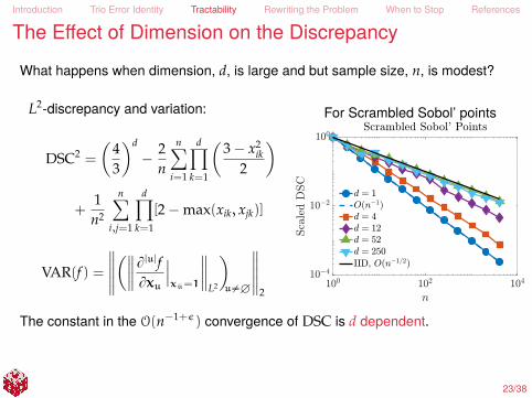
The Effect of Dimension on the Discrepancy
What happens when dimension, d, is large and but sample size, n, is modest?
L2-discrepancy and variation:
DSC2 =
(43
)d´
2n
nÿ
i=1
dź
k=1
(3´ x2
ik2
)
+1n2
nÿ
i,j=1
dź
k=1[2´max(xik, xjk)]
VAR(f ) =
∥∥∥∥∥(∥∥∥∥B|u|fBxu
∣∣∣x
su=1
∥∥∥∥L2
)u‰H
∥∥∥∥∥2
For Scrambled Sobol’ points
The constant in the O(n´1+ε) convergence of DSC is d dependent.
23/38

Introduction Trio Error Identity Tractability Rewriting the Problem When to Stop References
Pricing a Financial Derivative
µ´ µ̂ = ALN(f , ν´ ν̂)DSC(ν´ ν̂)VAR(f )
Paskov and Traub (1995) discovered that low discrepany sampling gavesignificant performance gains for pricing a Collaterlized Mortgage Obligation withd = 360
24/38

Introduction Trio Error Identity Tractability Rewriting the Problem When to Stop References
Pricing an Asian Option
µ =
ż
Rdpayoff(t)
exp(´ 1
2tTΣ´1t
)a
(2π)d det(Σ)dt =
ż
[0,1]df (x)dx
µ´ µ̂ = ALN(f , ν´ ν̂)DSC(ν´ ν̂)VAR(f )
For an Asian arithmetic meanoption, d = 12, µ « $13.1220
*
Scrambled Sobol’ achievesO(n´1) convergence for mod-est n provided that the Brow-nian motion is constructed byprincipal component analy-sis (PCA), rather than timestepping
25/38
Introduction Trio Error Identity Tractability Rewriting the Problem When to Stop References
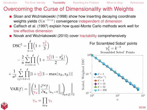
Overcoming the Curse of Dimensionality with WeightsSloan and Woźniakowski (1998) show how inserting decaying coordinateweights yields O(n´1+ε) convergence independent of dimensionCaflisch et al. (1997) explain how quasi-Monte Carlo methods work well forlow effective dimensionNovak and Woźniakowski (2010) cover tractability comprehensively
DSC2 =dź
k=1
(1 +
γ2k
3
)´
2n
nÿ
i=1
dź
k=1
(1 +
γ2k(1´ x2
ik)
2
)
+1n2
nÿ
i,j=1
dź
k=1[1+γ2
k(1´max(xik, xjk))]
VAR(f ) =
∥∥∥∥∥(
1γu
∥∥∥∥B|u|fBxu
∣∣∣x
su=1
∥∥∥∥L2
)u‰H
∥∥∥∥∥2
γu =ź
kPuγk
For Scrambled Sobol’ pointsγ2
k = k´3
26/38
Introduction Trio Error Identity Tractability Rewriting the Problem When to Stop References
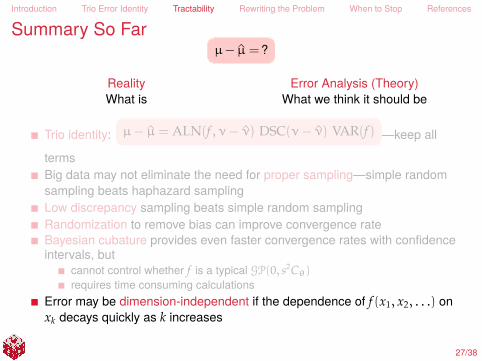
Summary So Farµ´ µ̂ = ?
Reality Error Analysis (Theory)What is What we think it should be
Trio identity: µ´ µ̂ = ALN(f , ν´ ν̂) DSC(ν´ ν̂) VAR(f ) —keep all
termsBig data may not eliminate the need for proper sampling—simple randomsampling beats haphazard samplingLow discrepancy sampling beats simple random samplingRandomization to remove bias can improve convergence rateBayesian cubature provides even faster convergence rates with confidenceintervals, but
cannot control whether f is a typical GP(0, s2Cθ)requires time consuming calculations
Error may be dimension-independent if the dependence of f (x1, x2, . . .) onxk decays quickly as k increases
27/38

Introduction Trio Error Identity Tractability Rewriting the Problem When to Stop References
Reducing VARµ =
ż
[0,1]dg(x)dx =
ż
[0,1]df (x)dx, ν = uniform
µ´ µ̂(g) = ALN(g, ν´ ν̂) DSC(ν´ ν̂) VAR(g)
µ´ µ̂(f ) = ALN(f , ν´ ν̂) DSC(ν´ ν̂) VAR(f )
Find f with ALN(f , ν´ ν̂)VAR(f ) ă ALN(g, ν´ ν̂)VAR(g).
Use PCA instead of timedifferencing for Brownian motionMultivariate normal probabilityControl variates:f (x) = g(x) + βT(µh ´ h(x))
Change of variables—importancesampling, antithetic variates, andthe tent transformation (H., 2002;Cristea et al., 2007)
28/38

Introduction Trio Error Identity Tractability Rewriting the Problem When to Stop References
Reducing VARµ =
ż
[0,1]dg(x)dx =
ż
[0,1]df (x)dx, ν = uniform
µ´ µ̂(g) = ALN(g, ν´ ν̂) DSC(ν´ ν̂) VAR(g)
µ´ µ̂(f ) = ALN(f , ν´ ν̂) DSC(ν´ ν̂) VAR(f )
Find f with ALN(f , ν´ ν̂)VAR(f ) ă ALN(g, ν´ ν̂)VAR(g).
Use PCA instead of timedifferencing for Brownian motionMultivariate normal probability
µ =
ż
[a,b]
exp(´ 1
2tTΣ´1t
)a
(2π)d det(Σ)dt
affine=
ż
[0,1]dg(x)dx
Genz (1993)=
ż
[0,1]df (x)dx
Control variates:f (x) = g(x) + βT(µh ´ h(x))
Change of variables—importancesampling, antithetic variates, andthe tent transformation (H., 2002;Cristea et al., 2007)
28/38

Introduction Trio Error Identity Tractability Rewriting the Problem When to Stop References
Reducing VARµ =
ż
[0,1]dg(x)dx =
ż
[0,1]df (x)dx, ν = uniform
µ´ µ̂(g) = ALN(g, ν´ ν̂) DSC(ν´ ν̂) VAR(g)
µ´ µ̂(f ) = ALN(f , ν´ ν̂) DSC(ν´ ν̂) VAR(f )
Find f with ALN(f , ν´ ν̂)VAR(f ) ă ALN(g, ν´ ν̂)VAR(g).
Use PCA instead of timedifferencing for Brownian motionMultivariate normal probabilityControl variates:f (x) = g(x) + βT(µh ´ h(x))β for low discrepancy sampling maybe different than for IID sampling (H.et al., 2005; Li, 2016)Change of variables—importancesampling, antithetic variates, andthe tent transformation (H., 2002;Cristea et al., 2007)
Asian Arithmetic Mean Callε = 0.0001
Timew/o control variates 4.00 sw/ Geometric MeanCall control variate
1.97 s
28/38

Introduction Trio Error Identity Tractability Rewriting the Problem When to Stop References
Reducing VARµ =
ż
[0,1]dg(x)dx =
ż
[0,1]df (x)dx, ν = uniform
µ´ µ̂(g) = ALN(g, ν´ ν̂) DSC(ν´ ν̂) VAR(g)
µ´ µ̂(f ) = ALN(f , ν´ ν̂) DSC(ν´ ν̂) VAR(f )
Find f with ALN(f , ν´ ν̂)VAR(f ) ă ALN(g, ν´ ν̂)VAR(g).
Use PCA instead of timedifferencing for Brownian motionMultivariate normal probabilityControl variates:f (x) = g(x) + βT(µh ´ h(x))
Change of variables—importancesampling, antithetic variates, andthe tent transformation (H., 2002;Cristea et al., 2007)
28/38

Introduction Trio Error Identity Tractability Rewriting the Problem When to Stop References
Controlling Costs for d Ñ∞E.g., for options based on continuously monitored assets:
µ = limdÑ∞µd, µd :=
ż
Xd
fd(x)νd(dx)
For µ « µ̂dhuge , how big should dhuge be?Computational cost of evaluating µ̂d is typically O(dn)
Break f into pieces:
f = fH + ft1u + ft2u + ¨ ¨ ¨+ ft1,2u + ¨ ¨ ¨ , fu depends only on xu, fd =ÿ
uĎ1:dfu
If fu gets small as maxtk : k P uu gets large, then can use fewer samples on thepieces of the function that are more expensive to evaluate
Multi-Level Monte Carlo Method: µ̂ = µ̂(fd1) + µ̂(fd2 ´ fd1) + ¨ ¨ ¨+ µ̂(fdL ´ fdL´1)expect VAR(fd` ´ fd`´1) Ó as ` Ò, (Heinrich, 2001; Giles, 2008; 2013; 2015; H. etal., 2010; Niu et al., 2011); Rhee and Glynn (2012) remove bias
Multivariate Decomposition Method: µ̂ = µ̂(fu1) + µ̂(fu2) + ¨ ¨ ¨+ µ̂(fuL)where the uk are the important sets of coordinate indices (Wasilkowski, 2013)
29/38

Introduction Trio Error Identity Tractability Rewriting the Problem When to Stop References
Summary So Farµ´ µ̂ = ?
Reality Error Analysis (Theory)What is What we think it should be
Trio identity: µ´ µ̂ = ALN(f , ν´ ν̂) DSC(ν´ ν̂) VAR(f ) —keep all
termsBig data may not eliminate the need for proper sampling—simple randomsampling beats haphazard samplingLow discrepancy sampling beats simple random samplingRandomization to remove bias can improve convergence rateBayesian cubature provides even faster convergence rates with confidenceintervals, but
cannot control whether f is a typical GP(0, s2Cθ)requires time consuming calculations
Error may be dimension-independent if the dependence of f (x1, x2, . . .) onxk decays quickly as k increasesChanging the integrand while leaving µ unchanged can reduce error
30/38

Introduction Trio Error Identity Tractability Rewriting the Problem When to Stop References
How Many Samples Are Needed?
Given an error tolerance, ε, how do we decide how many samples, n, are neededto make
|µ´ µ̂| = |ALN(f , ν´ ν̂)| DSC(ν´ ν̂) VAR(f ) ď ε
Bayesian cubature provides data-based confidence intervals for µ̂For IID Monte Carlo
The Central Limit Theorem is an asymptotic—not finite-sample—resultBut |µ´ µ̂| =
∣∣ALNR(f , ν´ ν̂)∣∣ std(f )/?n can be bounded with high
probability assuming a bound on kurt(f ) (H. et al., 2013; Bayer et al., 2014;Jiang, 2016)
For digital net (e.g., Sobol’) and integration lattice samplingIndependent replications present a trade-off between number of replicationsand number of samplesBut rigorous stopping criteria for a single sequence have been constructed interms of the discrete Fourier Walsh/complex exponential coefficients of f (H.and Jiménez Rugama, 2016; Jiménez Rugama and H., 2016; Li, 2016)
31/38
Introduction Trio Error Identity Tractability Rewriting the Problem When to Stop References
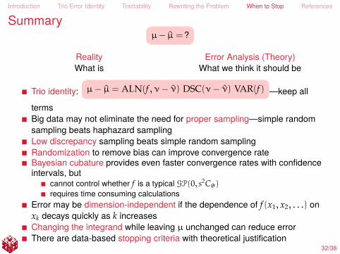
Summary
So Far
µ´ µ̂ = ?
Reality Error Analysis (Theory)What is What we think it should be
Trio identity: µ´ µ̂ = ALN(f , ν´ ν̂) DSC(ν´ ν̂) VAR(f ) —keep all
termsBig data may not eliminate the need for proper sampling—simple randomsampling beats haphazard samplingLow discrepancy sampling beats simple random samplingRandomization to remove bias can improve convergence rateBayesian cubature provides even faster convergence rates with confidenceintervals, but
cannot control whether f is a typical GP(0, s2Cθ)requires time consuming calculations
Error may be dimension-independent if the dependence of f (x1, x2, . . .) onxk decays quickly as k increasesChanging the integrand while leaving µ unchanged can reduce errorThere are data-based stopping criteria with theoretical justification
32/38

Thank you

Introduction Trio Error Identity Tractability Rewriting the Problem When to Stop References
References I
Anitescu, M., J. Chen, and M. Stein. 2016. An inversion-free estimating equation approach forGaussian process models, J. Comput. Graph. Statist.
Bayer, C., H. Hoel, E. von Schwerin, and R. Tempone. 2014. On nonasymptotic optimal stoppingcriteria in Monte Carlo Simulations, SIAM J. Sci. Comput. 36, A869–A885.
Caflisch, R. E., W. Morokoff, and A. Owen. 1997. Valuation of mortgage backed securities usingBrownian bridges to reduce effective dimension, J. Comput. Finance 1, 27–46.
Cools, R. and D. Nuyens (eds.) 2016. Monte Carlo and quasi-Monte Carlo methods: MCQMC,Leuven, Belgium, April 2014, Springer Proceedings in Mathematics and Statistics, vol. 163,Springer-Verlag, Berlin.
Cristea, L. L., J. Dick, G. Leobacher, and F. Pillichshammer. 2007. The tent transformation canimprove the convergence rate of quasi-Monte Carlo algorithms using digital nets, Numer. Math. 105,413–455.
Diaconis, P. 1988. Bayesian numerical analysis, Statistical decision theory and related topics IV,Papers from the 4th Purdue symp., West Lafayette, Indiana 1986, pp. 163–175.
Dick, J. 2008. Walsh spaces containing smooth functions an quasi-monte carlo rules of arbitrary highorder, SIAM J. Numer. Anal. 46, no. 1519–1553.
34/38

Introduction Trio Error Identity Tractability Rewriting the Problem When to Stop References
References IIDick, J., F. Y. Kuo, G. W. Peters, and I. H. Sloan (eds.) 2013. Monte Carlo and quasi-Monte Carlomethods 2012, Springer Proceedings in Mathematics and Statistics, vol. 65, Springer-Verlag, Berlin.
Dick, J. and F. Pillichshammer. 2010. Digital nets and sequences: Discrepancy theory andquasi-Monte Carlo integration, Cambridge University Press, Cambridge.
Genz, A. 1993. Comparison of methods for the computation of multivariate normal probabilities,Computing Science and Statistics 25, 400–405.
Giles, M. 2013. Multilevel Monte Carlo methods, Monte Carlo and quasi-Monte Carlo methods 2012.
. 2015. Multilevel monte carlo methods, Acta Numer. 24, no. 259–328.
Giles, M. B. 2008. Multilevel Monte Carlo path simulation, Oper. Res. 56, 607–617.
Griebel, M., F. Y. Kuo, and I. H. Sloan. 2010. The smoothing effect of the ANOVA decomposition, J.Complexity 26, 523–551.
. 2016+. The ANOVA decomposition of a non-smooth function of infinitely many variables canhave every term smooth, Math. Comp. in press.
Heinrich, S. 2001. Multilevel Monte Carlo methods, Large-scale scientific computing, Thirdinternational conference, LSSC 2001, pp. 58–67.
Heinrich, S., F. J. H., and R. X. Yue. 2004. Optimal quadrature for Haar wavelet spaces, Math. Comp.73, 259–277.
35/38

Introduction Trio Error Identity Tractability Rewriting the Problem When to Stop References
References IIIH., F. J. 1998. A generalized discrepancy and quadrature error bound, Math. Comp. 67, 299–322.
. 1999. Goodness-of-fit statistics, discrepancies and robust designs, Statist. Probab. Lett. 44,73–78.
. 2000. What affects the accuracy of quasi-Monte Carlo quadrature?, Monte Carlo andquasi-Monte Carlo methods 1998, pp. 16–55.
. 2002. Obtaining O(N´2+ε) convergence for lattice quadrature rules, Monte Carlo andquasi-Monte Carlo methods 2000, pp. 274–289.
H., F. J., L. Jiang, Y. Liu, and A. B. Owen. 2013. Guaranteed conservative fixed width confidenceintervals via Monte Carlo sampling, Monte Carlo and quasi-Monte Carlo methods 2012, pp. 105–128.
H., F. J. and Ll. A. Jiménez Rugama. 2016. Reliable adaptive cubature using digital sequences,Monte Carlo and quasi-Monte Carlo methods: MCQMC, Leuven, Belgium, April 2014, pp. 367–383.arXiv:1410.8615 [math.NA].
H., F. J., C. Lemieux, and A. B. Owen. 2005. Control variates for quasi-Monte Carlo, Statist. Sci. 20,1–31.
H., F. J., T. Müller-Gronbach, B. Niu, and K. Ritter. 2010. Multi-level Monte Carlo algorithms forinfinite-dimensional integration on RN, J. Complexity 26, 229–254.
H., F. J. and R. X. Yue. 2000. The mean square discrepancy of scrambled (t, s)-sequences, SIAM J.Numer. Anal. 38, 1089–1112.
36/38

Introduction Trio Error Identity Tractability Rewriting the Problem When to Stop References
References IV
Hlawka, E. 1961. Funktionen von beschränkter Variation in der Theorie der Gleichverteilung, Ann.Mat. Pura Appl. 54, 325–333.
Jiang, L. 2016. Guaranteed adaptive Monte Carlo methods for estimating means of randomvariables, Ph.D. Thesis.
Jiménez Rugama, Ll. A. and F. J. H. 2016. Adaptive multidimensional integration based on rank-1lattices, Monte Carlo and quasi-Monte Carlo methods: MCQMC, Leuven, Belgium, April 2014,pp. 407–422. arXiv:1411.1966.
Li, D. 2016. Reliable quasi-Monte Carlo with control variates, Master’s Thesis.
Meng, X. 2016+. Statistical paradises and paradoxes in big data. in preparation.
Niederreiter, H. 1992. Random number generation and quasi-Monte Carlo methods, CBMS-NSFRegional Conference Series in Applied Mathematics, SIAM, Philadelphia.
Niu, B., F. J. H., T. Müller-Gronbach, and K. Ritter. 2011. Deterministic multi-level algorithms forinfinite-dimensional integration on RN, J. Complexity 27, 331–351.
Novak, E. and H. Woźniakowski. 2010. Tractability of multivariate problems Volume ii: Standardinformation for functionals, EMS Tracts in Mathematics, European Mathematical Society, Zürich.
O’Hagan, A. 1991. Bayes-Hermite quadrature, J. Statist. Plann. Inference 29, 245–260.
37/38

Introduction Trio Error Identity Tractability Rewriting the Problem When to Stop References
References V
Owen, A. B. 1997. Scrambled net variance for integrals of smooth functions, Ann. Stat. 25,1541–1562.
Paskov, S. and J. Traub. 1995. Faster valuation of financial derivatives, J. Portfolio Management 22,113–120.
Rasmussen, C. E. and Z. Ghahramani. 2003. Bayesian Monte Carlo, Advances in Neural InformationProcessing Systems, pp. 489–496.
Rhee, C. and P. Glynn. 2012. A new approach to unbiased estimation for SDE’s, Proceedings of the2012 winter simulation conference.
Ritter, K. 2000. Average-case analysis of numerical problems, Lecture Notes in Mathematics,vol. 1733, Springer-Verlag, Berlin.
Sloan, I. H. and H. Woźniakowski. 1998. When are quasi-Monte Carlo algorithms efficient for highdimensional integrals?, J. Complexity 14, 1–33.
Wasilkowski, G. W. 2013. On tractability of linear tensor product problems for ∞-variate classes offunctions, J. Complexity 29, 351–369.
38/38