MBMG 638-Lower Beaverhead Study Area · HYDROGEOLOGIC INVESTIGATION OF THE LOWER BEAVERHEAD STUDY...
86
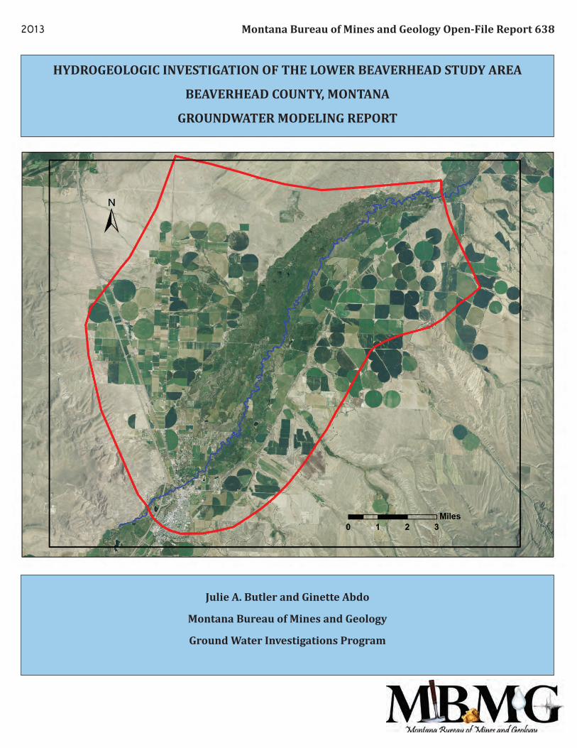
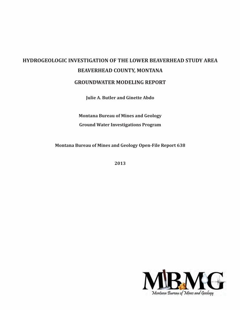
HYDROGEOLOGIC INVESTIGATION OF THE LOWER BEAVERHEAD STUDY AREA BEAVERHEAD COUNTY, MONTANA GROUNDWATER MODELING REPORT Julie A. Butler and Ginette Abdo Montana Bureau of Mines and Geology Ground Water Investigations Program Montana Bureau of Mines and Geology Open-File Report 638 2013
Transcript of MBMG 638-Lower Beaverhead Study Area · HYDROGEOLOGIC INVESTIGATION OF THE LOWER BEAVERHEAD STUDY...
HYDROGEOLOGIC INVESTIGATION OF THE LOWER BEAVERHEAD STUDY AREA
BEAVERHEAD COUNTY, MONTANA
GROUNDWATER MODELING REPORT
Julie A. Butler and Ginette Abdo
Montana Bureau of Mines and Geology
Ground Water Investigations Program
Montana Bureau of Mines and Geology Open-File Report 6382013

HYDROGEOLOGIC INVESTIGATION OF THE LOWER BEAVERHEAD STUDY AREA
BEAVERHEAD COUNTY, MONTANA
GROUNDWATER MODELING REPORT
Montana Bureau of Mines and Geology Open-File Report 638
2013
Julie A. Butler and Ginette Abdo
Montana Bureau of Mines and Geology
Ground Water Investigations Program

v
Montana Bureau of Mines and Geology Open-File Report 638
TABLE OF CONTENTS
Introduction ......................................................................................................................................................................... 1 Report Purpose ............................................................................................................................................................ 1 General Setting ............................................................................................................................................................. 1 Climate ............................................................................................................................................................................. 1 Physiography ................................................................................................................................................................. 3 Man-Made Hydrologic Features ............................................................................................................................ 4 Model Objectives ......................................................................................................................................................... 4Conceptual Model ............................................................................................................................................................... 4 Geologic Framework .................................................................................................................................................. 5 Hydrogeologic Units ................................................................................................................................................... 7 Alluvial Aquifer ..................................................................................................................................................... 8 Tertiary Sediment Aquifer................................................................................................................................ 10 Volcanic Rock Aquifer ........................................................................................................................................ 12 Groundwater Flow System ...................................................................................................................................... 13 Vertical Gradients ................................................................................................................................................ 16 Hydrologic Boundaries ............................................................................................................................................. 18 Aquifer Properties ...................................................................................................................................................... 18 Tertiary Sediment Aquifer Test ...................................................................................................................... 18 Volcanic Rock Aquifer Test ............................................................................................................................... 19 Alluvial Aquifer Tests ......................................................................................................................................... 21 Summary of Hydraulic Properties ................................................................................................................ 21 Sources and Sinks ........................................................................................................................................................ 21 Groundwater Budget ................................................................................................................................................. 21Computer Code .................................................................................................................................................................... 24Groundwater Flow Model Construction ................................................................................................................... 25 Model Grid ...................................................................................................................................................................... 25 Hydraulic Parameters ................................................................................................................................................ 27 Boundary Conditions ................................................................................................................................................. 27 Model Borders ....................................................................................................................................................... 27 Surface-Water Bodies ......................................................................................................................................... 27 Irrigation Field Recharge .................................................................................................................................. 28 Well Withdrawals ................................................................................................................................................. 28Calibration ............................................................................................................................................................................. 29 Selection of Calibration Targets ............................................................................................................................ 29 Steady-State Calibration ........................................................................................................................................... 30 Transient Calibration ................................................................................................................................................. 33 Sensitivity Analysis ..................................................................................................................................................... 36 Model Veri ication ....................................................................................................................................................... 36Predictive Simulations ...................................................................................................................................................... 37 Scenario 1 ....................................................................................................................................................................... 38 Scenario 2 ....................................................................................................................................................................... 38 Scenario 3 ....................................................................................................................................................................... 39 Scenario 4 ....................................................................................................................................................................... 41 Canal Seepage Scenarios .......................................................................................................................................... 41 Scenarios 5 and 6 ................................................................................................................................................. 41 Scenario 7 ................................................................................................................................................................ 47Summary and Conclusions ............................................................................................................................................. 48
vi
Butler and Abdo, 2013
Assumptions and Limitations ...........................................................................................................................48 Model Predictions ..................................................................................................................................................50 Recommendations .................................................................................................................................................52References ........................................................................................................................................................................ 52Appendix A. Model File Index ................................................................................................................................... 55Appendix B. Estimating Irrigation Recharge in the Groundwater Budget ............................................ 61Appendix C. Estimating Well Withdrawals in the Groundwater Budget ............................................... 65Appendix D. NRCS Irrigation Water Requirements—Crop Data Summaries ...................................... 69
FIGURESFigure 1. Site location and physiography ...............................................................................................................2Figure 2. Study area .........................................................................................................................................................3Figure 3. Deviation from annual average precipitation in Dillon, 1900–2010 ......................................4 Figure 4. Beaverhead River and tributaries of interest in the model .........................................................5Figure 5. Study area geology ........................................................................................................................................6Figure 6. Cross section through the lower Beaverhead River basin ...........................................................8Figure 7. Exposures of the primary hydrogeologic units in the study area ............................................9Figure 8. Location of sedimentary bedrock outcrop, observed August 4, 2010 .................................10Figure 9. Groundwater monitoring sites, including MBMG well installations ....................................11Figure 10. 3D cross sections through loodplain .............................................................................................11Figure 11. Estimation of the volcanic rock aquifer extent ...........................................................................12Figure 12. Groundwater low system—bench potentiometric surface ..................................................13Figure 13. Groundwater low system— loodplain (shallow alluvial) potentiometric surface ....14Figure 14. Groundwater levels in luenced by irrigation practices ..........................................................15Figure 15. Vertical gradient monitoring sites ....................................................................................................16Figure 16. Site A and B hydrographs ..........................................................................................................................Figure 17. Site F hydrographs ..................................................................................................................................18Figure 18. Tertiary sediment aquifer test site ..................................................................................................19Figure 19. Volcanic rock aquifer test site ...........................................................................................................20Figure 20. Active cell coverage in the Lower Beaverhead model ..............................................................25 Figure 21. Model cross section through Row 237 of the model ................................................................26Figure 22. Model boundary conditions ................................................................................................................28Figure 23. Irrigation ield recharge in the model ...........................................................................................29Figure 24. Hydraulic conductivity array generated by steady-state calibration of the model .....32Figure 25. Potentiometric surface generated by steady-state calibration of the model .................33 Figure 26. Computed vs. observed hydraulic head in the steady-state model ...................................34Figure 27. Computed vs. observed heads of selected wells from the 2010 transient model .......35Figure 28. RMS error caused by changing K and recharge values ............................................................37Figure 29. Potentiometric surface and head residuals from a 50% decrease in K values .............38Figure 30. Potentiometric surface and head residuals from a 50% increase in recharge
values ............................................................................................................................................................39Figure 31. Well locations in pumping and canal-seepage scenarios .......................................................41Figure 32. Stream depletion in the inal year of scenario 2 ........................................................................42Figure 33. Spatial distribution of stream depletion in Beaverhead River during year 20
of scenario 2 ..............................................................................................................................................43Figure 34. Stream depletion in the inal year of scenario 3 ........................................................................44Figure 35. Stream depletion in Beaverhead River throughout scenario 3............................................45Figure 36. Drawdown in wells OW-1 and OW-2 in scenario 3 ...................................................................45Figure 37. Stream depletion in the inal year of scenario 4 ........................................................................46
vii
Montana Bureau of Mines and Geology Open-File Report 638
Figure 38. Base low to Willard and Black Sloughs in scenarios 1, 3, and 5 ..........................................47Figure 39. Base low to Willard and Black Sloughs in scenarios 1, 3, and 6 ..........................................48Figure 40. Base low to Willard and Black Sloughs in scenarios 1, 3, and 7 ..........................................49Figure 41. Base low to Beaverhead River in scenarios 1, 3, and 7 ...........................................................50Figure 42. Plan view of maximum drawdown in scenarios 3 and 7 ........................................................51
TABLESTable 1. Ranges of aquifer property values based on aquifer test results in the study area .........21Table 2. Hydraulic conductivity values used in other western Montana large-area
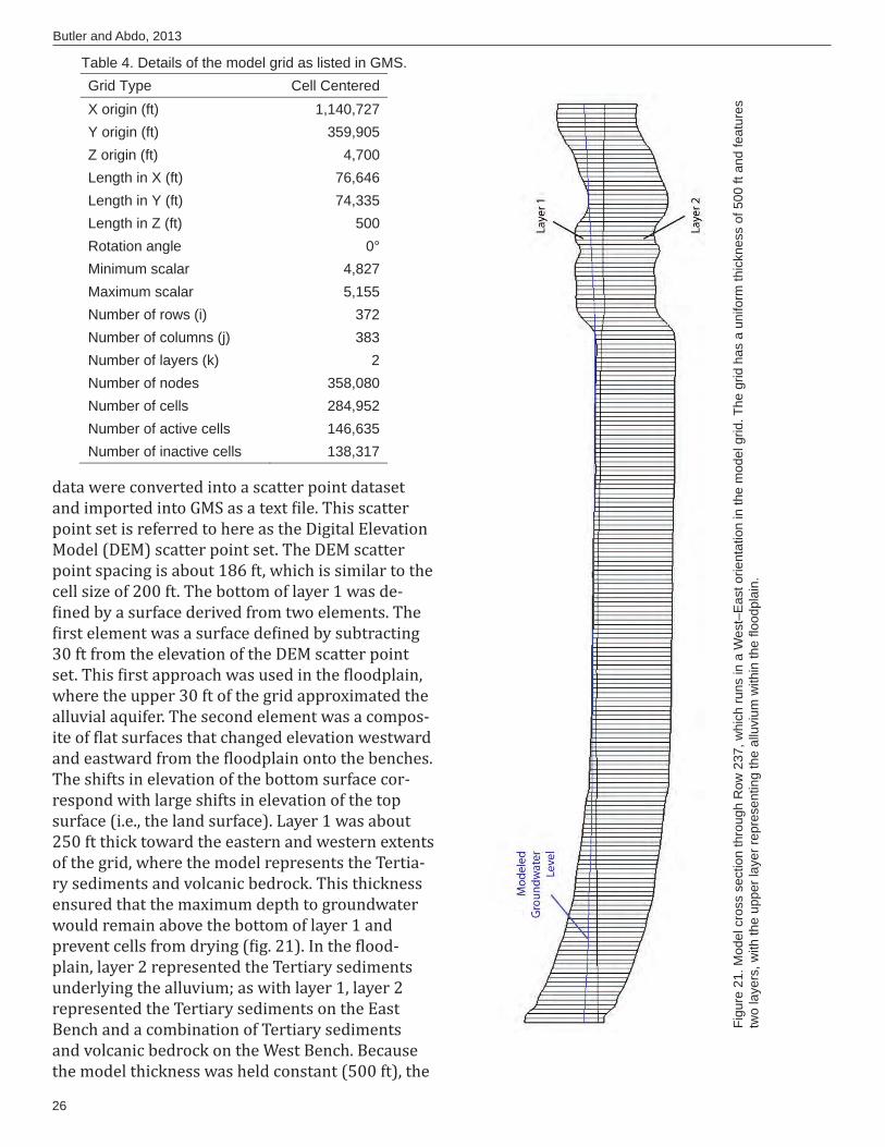
groundwater models ...................................................................................................................................22Table 3. Comparison of ield-estimated and model aquifer property values ......................................22Table 4. Details of the model grid as listed in GMS .........................................................................................26Table 5. Base low comparison between ield estimates and model results .........................................34Table 6. Stress periods and time steps in the 2010 transient model run ..............................................35Table 7. Water budget values in the steady-state and transient versions of the model ..................36Table 8. Summary of pumping and canal seepage scenarios ......................................................................40

1
Montana Bureau of Mines and Geology Open-File Report 638
INTRODUCTION The main economy in the lower Beaverhead
River basin is agriculture, which is dependent on groundwater and surface-water irrigation. The basin was closed to new surface-water appropria-tions by Legislative authority effective April 1, 1993, as part of the Jefferson–Madison River Basin closure [Montana Department of Natural Resources (DNRC), 2003]. In a closed basin, the DNRC may not grant new surface-water rights except in re-stricted circumstances. This closure, combined with increased irrigation demands, resulted in an increased number of high-volume irrigation wells. However, a 2006 Montana Supreme Court decision recognized impacts to stream low by pre-stream capture of tributary groundwater, which effectively closed the basin to new groundwater develop-ment (Montana Supreme Court, 2006). In 2007, the Montana Legislature passed House Bill 831 in an attempt to improve this situation; the bill required a hydrogeologic assessment to determine whether a new well would result in a “net depletion” of surface water and affect a prior appropriator. If depletion of surface water was shown, the appli-cant would then have to submit a plan to mitigate the depletion.
Applications for new well permits have led to con licts between senior surface-water rights hold-ers and junior groundwater rights holders. A com-mon objection to the well permits is that ground-water withdrawals will reduce stream low and lower groundwater levels. Based on House Bill 831, applications for new well permits must address stream depletion and groundwater drawdown in a scienti ically sound manner.
The Lower Beaverhead groundwater investiga-tion (Abdo and others, 2013) was conducted to build on previous hydrologic and hydrogeologic studies in the area [Montana Bureau of Mines and Geology (MBMG), 2008; Weight and Snyder, 2007; U.S. Bureau of Reclamation, 2008; H. Sessoms and J. Bauder, written commun., 2007]. The primary objectives were to determine if groundwater draw-down and stream depletion were occurring due to high-capacity irrigation well withdrawals, and to evaluate possible impacts to streams from future groundwater development. Particular attention was given to the West Bench area, in part because stream depletion was examined on the East Bench
in a previous study (MBMG, 2008) and because several West Bench well-permit applications were awaiting approval for some time. The study in-volved aquifer testing, groundwater and surface-water monitoring, well installations, water budget analyses, and an evaluation of groundwater-level trends. Results of the investigation were intended to provide a scienti ic basis in which to help land-owners and governing agencies make informed management decisions. Other interest groups could also bene it from the study’s baseline data in their future work, such as watershed health improve-ment projects.
Report PurposeThis report provides documentation of the
procedures and assumptions inherent in the model and communicates the indings of the model; it is intended to allow the model to be evaluated and used by others. All iles needed to operate the groundwater model are posted to the program website (http://www.mbmg.mtech.edu/gwip/gwip.asp). The iles are intended to enable quali ied individuals to use the model developed by GWIP to test speci ic scenarios of interest, or to provide a starting point for site-speci ic analysis.
General SettingThe Lower Beaverhead study area is located in
southwestern Montana between Dillon and Bea-verhead Rock ( igs. 1, 2) and covers approximately 110 square miles. The study area encompasses the lower portion of the Beaverhead River and its loodplain, as well as the East Bench and West Bench ( ig. 2).
ClimateThe long-term average annual precipitation in
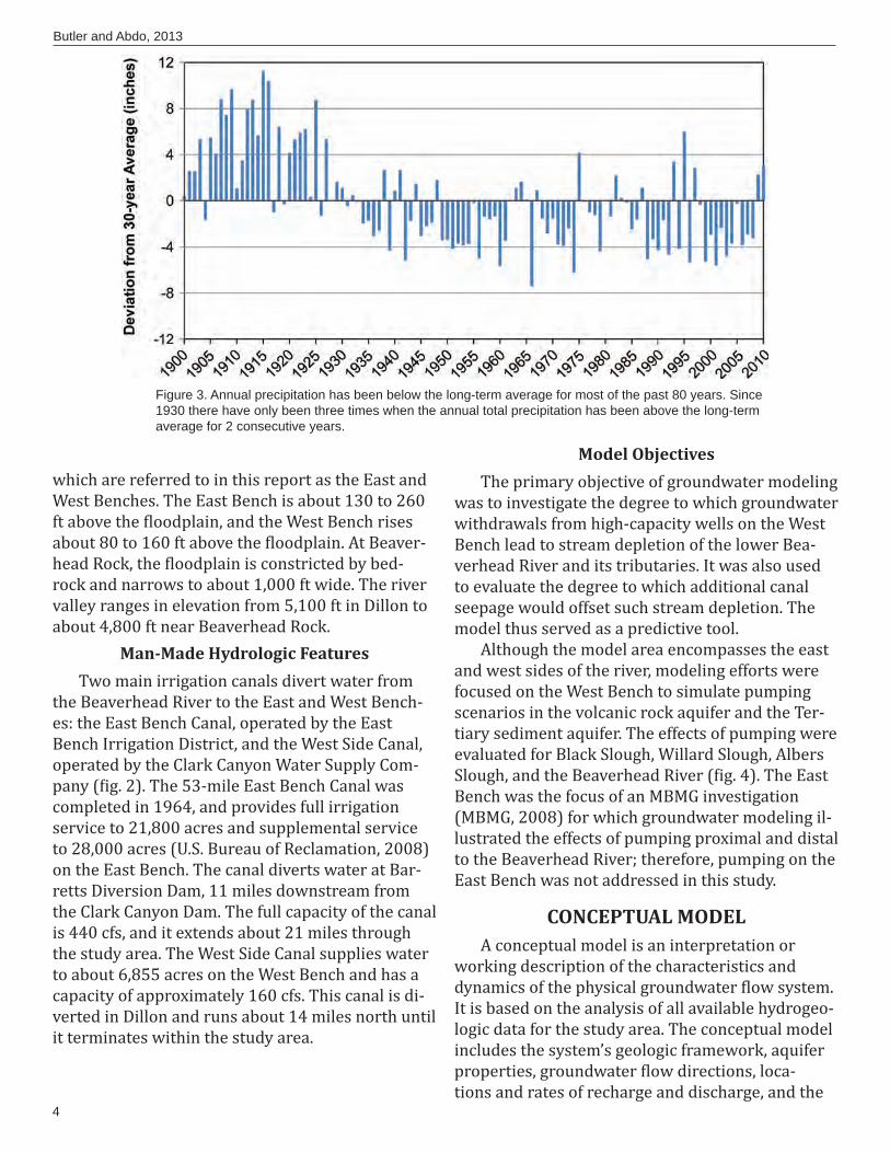
Dillon is 13.17 in based on a 111-year period of record. The short-term annual average is 11.46 in based on the past 30 years [Western Regional Cli-mate Center (WRCC), 2011]. In general, precipita-tion was above average from 1900 to 1930 ( ig. 3). From the 1930s through 2007, most of the annual precipitation was below the long-term average; only 17 years of that 77-year period showed above-average precipitation. With the exception of the past 2 years, the last decade has seen below-aver-age precipitation, and in 7 of those years the devia-tion below normal was 3 in or more. Nearly half of the annual rainfall fell between April and July
2
Butler and Abdo, 2013
of each year. The average maximum temperature over the period of record occurred in July (83.3°F), and the average minimum temperature occurred in January (12.6°F).
The average annual snowfall in Dillon is 37.3 in, based on the 116-year period of record from the University of Montana–Western weather station
(WRCC, 2011). Almost 90% of this snow fell be-tween November and April of each year. A SNOTEL (SNOpack TELemetry) station (Mule Creek Station #656) is located about 20 miles northwest of Dillon at an elevation of 8,300 ft. Snow-water equivalent data (31-year record) indicate the annual aver-age maximum to be 17.36 in at this site (SNOTEL,
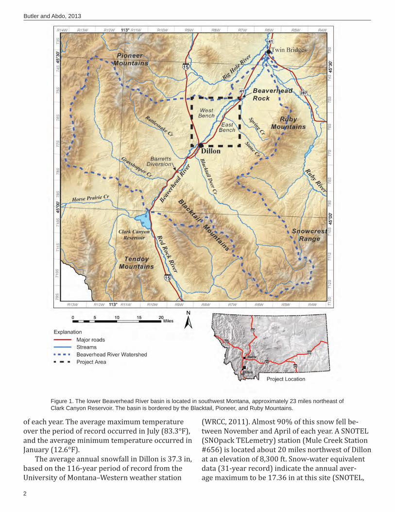
Figure 1. The lower Beaverhead River basin is located in southwest Montana, approximately 23 miles northeast of Clark Canyon Reservoir. The basin is bordered by the Blacktail, Pioneer, and Ruby Mountains.
3
Montana Bureau of Mines and Geology Open-File Report 638
2011). The average date of the maximum snow-water equivalent is May 11th, and the average date of snowpack disappearance is June 15th. Therefore, the snowpack takes an average of 35 days to melt completely.
PhysiographyThe Beaverhead River drainage encompasses an
area of about 2,895 square miles below the Clark Canyon Reservoir, 23 miles southwest of Dillon, Montana ( ig. 1). The reservoir receives water from Red Rock River and Horse Prairie Creek. The Bea-verhead River lows northeast through the Beaver-head Canyon and into the Beaverhead River Valley for about 45 miles until its con luence with the Big Hole and Ruby Rivers near Twin Bridges. There it forms the headwaters of the Jefferson River, a tribu-tary to the Missouri River.
The basin is bounded by the Pioneer Mountains to the west, the Ruby Mountains to the east, and
the Tendoy, Snowcrest, and Blacktail Ranges to the south ( ig. 1). Major tributaries to the Beaverhead River include Grasshopper Creek, Blacktail Deer Creek, and Rattlesnake Creek. Grasshopper Creek lows toward the southeast and joins the Beaver-
head River above Barretts Diversion. Blacktail Deer Creek lows to the northwest in a northwest–south-east-trending valley that is nearly at right angles to the Beaverhead River Valley; it joins the Beaver-head River near Dillon. Rattlesnake Creek lows to-wards the southeast and also joins the Beaverhead River near Dillon. Within the study area, extending north of Dillon to Beaverhead Rock ( ig. 2), Stone Creek and Spring Creek low northwest into the Beaverhead River from the Ruby Mountains.
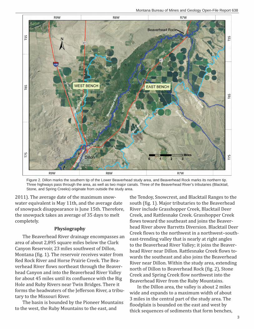
In the Dillon area, the valley is about 2 miles wide and expands to a maximum width of about 3 miles in the central part of the study area. The loodplain is bounded on the east and west by
thick sequences of sediments that form benches,
Figure 2. Dillon marks the southern tip of the Lower Beaverhead study area, and Beaverhead Rock marks its northern tip. Three highways pass through the area, as well as two major canals. Three of the Beaverhead River’s tributaries (Blacktail, Stone, and Spring Creeks) originate from outside the study area.
4
Butler and Abdo, 2013
which are referred to in this report as the East and West Benches. The East Bench is about 130 to 260 ft above the loodplain, and the West Bench rises about 80 to 160 ft above the loodplain. At Beaver-head Rock, the loodplain is constricted by bed-rock and narrows to about 1,000 ft wide. The river valley ranges in elevation from 5,100 ft in Dillon to about 4,800 ft near Beaverhead Rock.
Man-Made Hydrologic FeaturesTwo main irrigation canals divert water from
the Beaverhead River to the East and West Bench-es: the East Bench Canal, operated by the East Bench Irrigation District, and the West Side Canal, operated by the Clark Canyon Water Supply Com-pany ( ig. 2). The 53-mile East Bench Canal was completed in 1964, and provides full irrigation service to 21,800 acres and supplemental service to 28,000 acres (U.S. Bureau of Reclamation, 2008) on the East Bench. The canal diverts water at Bar-retts Diversion Dam, 11 miles downstream from the Clark Canyon Dam. The full capacity of the canal is 440 cfs, and it extends about 21 miles through the study area. The West Side Canal supplies water to about 6,855 acres on the West Bench and has a capacity of approximately 160 cfs. This canal is di-verted in Dillon and runs about 14 miles north until it terminates within the study area.
Model ObjectivesThe primary objective of groundwater modeling
was to investigate the degree to which groundwater withdrawals from high-capacity wells on the West Bench lead to stream depletion of the lower Bea-verhead River and its tributaries. It was also used to evaluate the degree to which additional canal seepage would offset such stream depletion. The model thus served as a predictive tool.
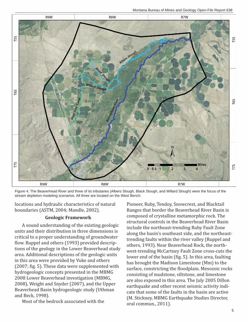
Although the model area encompasses the east and west sides of the river, modeling efforts were focused on the West Bench to simulate pumping scenarios in the volcanic rock aquifer and the Ter-tiary sediment aquifer. The effects of pumping were evaluated for Black Slough, Willard Slough, Albers Slough, and the Beaverhead River ( ig. 4). The East Bench was the focus of an MBMG investigation (MBMG, 2008) for which groundwater modeling il-lustrated the effects of pumping proximal and distal to the Beaverhead River; therefore, pumping on the East Bench was not addressed in this study.
CONCEPTUAL MODELA conceptual model is an interpretation or
working description of the characteristics and dynamics of the physical groundwater low system. It is based on the analysis of all available hydrogeo-logic data for the study area. The conceptual model includes the system’s geologic framework, aquifer properties, groundwater low directions, loca-tions and rates of recharge and discharge, and the
Figure 3. Annual precipitation has been below the long-term average for most of the past 80 years. Since 1930 there have only been three times when the annual total precipitation has been above the long-term average for 2 consecutive years.
5
Montana Bureau of Mines and Geology Open-File Report 638
locations and hydraulic characteristics of natural boundaries (ASTM, 2004; Mandle, 2002).
Geologic FrameworkA sound understanding of the existing geologic
units and their distribution in three dimensions is critical to a proper understanding of groundwater low. Ruppel and others (1993) provided descrip-
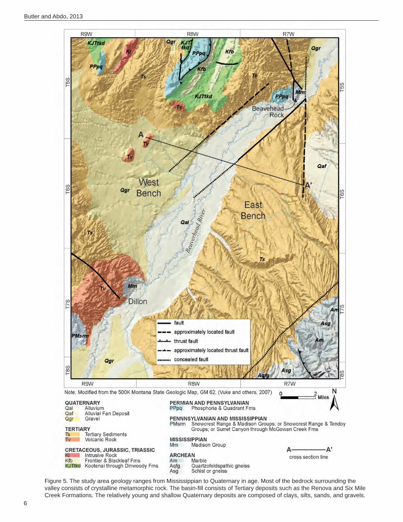
tions of the geology in the Lower Beaverhead study area. Additional descriptions of the geologic units in this area were provided by Vuke and others (2007; ig. 5). These data were supplemented with hydrogeologic concepts presented in the MBMG 2008 Lower Beaverhead investigation (MBMG, 2008), Weight and Snyder (2007), and the Upper Beaverhead Basin hydrogeologic study (Uthman and Beck, 1998).
Most of the bedrock associated with the
Pioneer, Ruby, Tendoy, Snowcrest, and Blacktail Ranges that border the Beaverhead River Basin is composed of crystalline metamorphic rock. The structural controls in the Beaverhead River Basin include the northeast-trending Ruby Fault Zone along the basin’s southeast side, and the northeast-trending faults within the river valley (Ruppel and others, 1993). Near Beaverhead Rock, the north-west-trending McCartney Fault Zone cross-cuts the lower end of the basin ( ig. 5). In this area, faulting has brought the Madison Limestone (Mm) to the surface, constricting the loodplain. Mesozoic rocks consisting of mudstone, siltstone, and limestone are also exposed in this area. The July 2005 Dillon earthquake and other recent seismic activity indi-cate that some of the faults in the basin are active (M. Stickney, MBMG Earthquake Studies Director, oral commun., 2011).
Figure 4. The Beaverhead River and three of its tributaries (Albers Slough, Black Slough, and Willard Slough) were the focus of the stream depletion modeling scenarios. All three are located on the West Bench.
6
Butler and Abdo, 2013
Figure 5. The study area geology ranges from Mississippian to Quaternary in age. Most of the bedrock surrounding the valley consists of crystalline metamorphic rock. The basin-fi ll consists of Tertiary deposits such as the Renova and Six Mile Creek Formations. The relatively young and shallow Quaternary deposits are composed of clays, silts, sands, and gravels.

7
Montana Bureau of Mines and Geology Open-File Report 638
The basin- ill between Dillon and Beaverhead Rock may be about 1,000 ft thick (R. Thomas, Pro-fessor of Geology, University of Montana Western, oral commun., 2011). The bulk of this basin- ill con-sists of Tertiary deposits, namely the Renova and Six Mile Creek Formations of the Bozeman Group, which are the main Tertiary units in southwestern Montana. The Renova volcanic and volcanoclastic sequence was deposited during the early to middle Miocene in a broad continuous wedge across the basin over a low-relief loodplain. The depositional sequence was overwhelmed with volcanically derived sediment, which typically is ine-grained material with low permeability. Non-volcanic facies include sandstone, carbonaceous shale, lignite, and limestone deposited in lakes and streams (Alt and Hyndman, 1986).
During the middle Miocene, the basin was seg-mented into several grabens by basin-and-range style faulting. Sequences of non-volcanic and vol-canic sediments known as the Six Mile Creek For-mation illed the Beaverhead and other grabens in southwest Montana during the middle Miocene to late Pliocene. The Six Mile Creek Formation is gen-erally coarser-grained than the underlying Renova Formation and consists of mudstone, siltstone, conglomerate with local occurrences of limestone, volcanic fallout ash, pyroclastic ash low tuffs, fallout tuffs, and basalt lows. The Six Mile Creek Formation is generally thickest near the axis of the valleys and thins in the uplands.
Also during the Tertiary Period, volcanic low deposits formed as magma intruded through older rocks and lowed at the surface. The sur icial de-posits inter ingered with and were overlain by the Tertiary sediments. The unit consists mainly of rhyodacite, an extrusive volcanic rock, and ranges from purple-brown to gray-brown in color. Within the lower Beaverhead basin, it is found west of Dil-lon and in northern portions of the West Bench.
During the Quaternary Period, clays, silts, sands, and gravels were deposited over the Tertiary for-mations of the Beaverhead basin. These deposits are primarily found in the valley bottoms as allu-vium, and in the uplands as alluvial fans and land-slide deposits.
Hydrogeologic UnitsThe Lower Beaverhead basin’s hydrogeologic
units were discerned from the geologic framework, ield observations, and well logs. Well logs from the
MBMG Groundwater Information Center (GWIC) include such information as the well location, lithologic descriptions, and well-completion details. The GWIC logs were reviewed to help identify the primary types and locations of aquifers in the study area. Lithologic descriptions in each log were com-pared with those in surrounding well logs and with geologic maps.
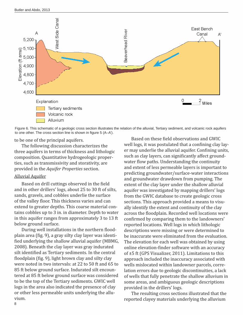
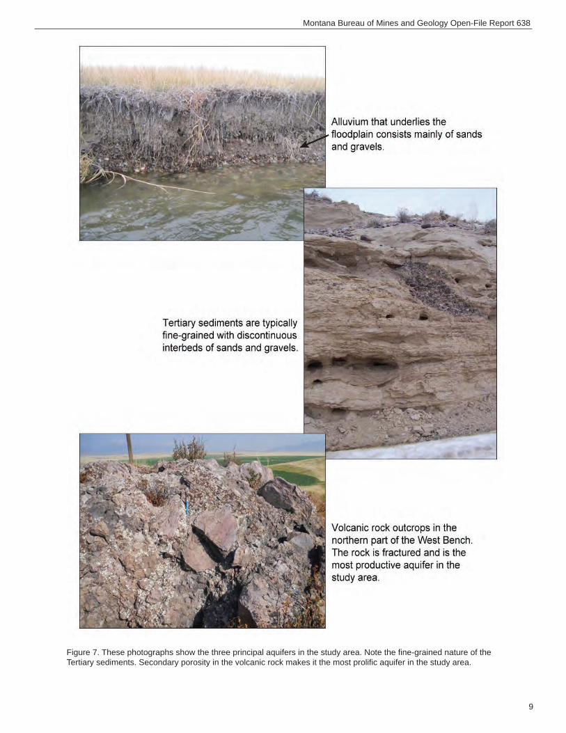
The three principal aquifers identi ied in the study area are: the alluvial aquifer that forms the sur icial deposit in the Beaverhead River Valley; the Tertiary sediment aquifer that underlies the alluvi-um and also comprises the East and West Benches; and the volcanic rock aquifer on the northern West Bench ( ig. 6). Outcrops of the alluvium, Tertiary sediments, and volcanic rock are shown in igure 7. The geologic map for the area ( ig. 5) indicates Quaternary sands and gravels (Qgr) overlying the Tertiary sediments on the West Bench. The Qua-ternary/Tertiary contact on the West Bench is not well de ined, and sediments deposited during this period in time were probably formed under similar conditions. For this reason, the Quaternary sedi-ments that blanket the West Bench are considered part of the Tertiary sediment aquifer within the study area.
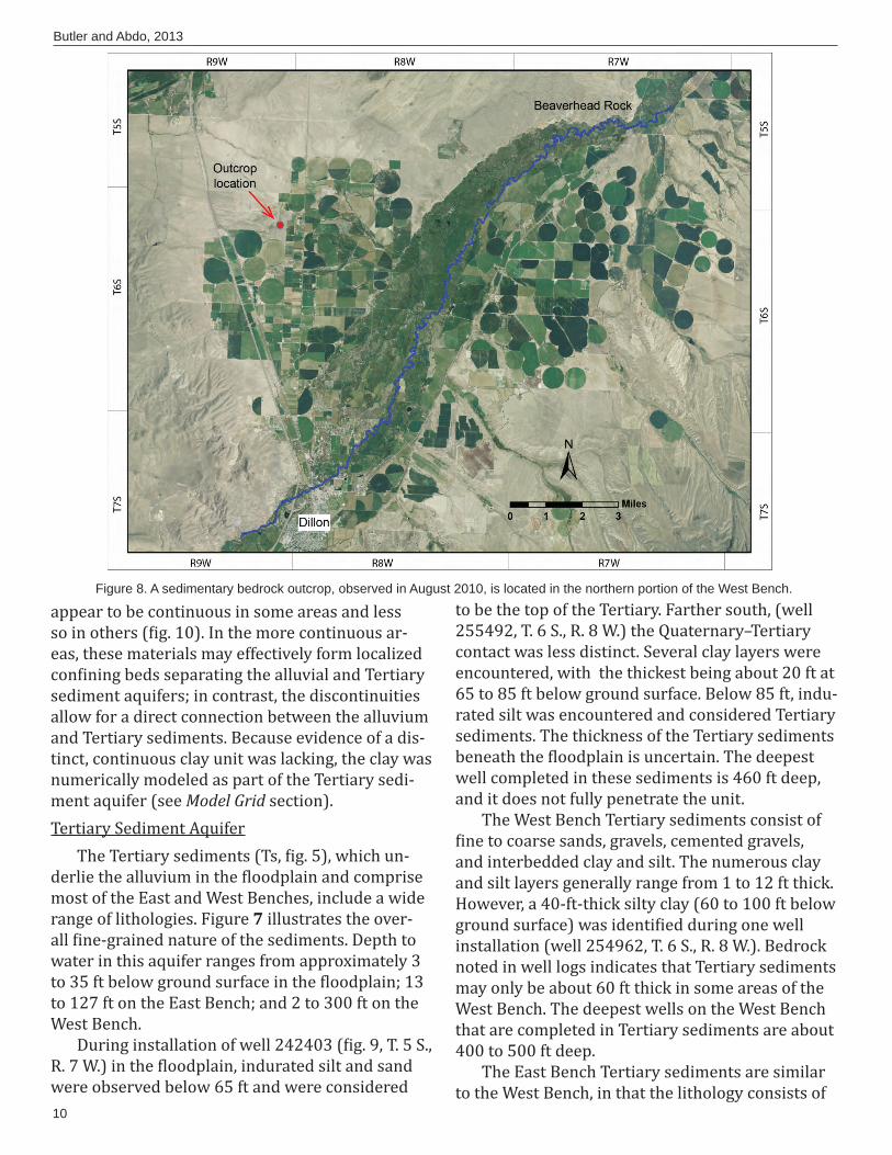
Field observations and GWIC well logs have suggested the presence of a fourth aquifer located near the study area’s western boundary, composed of sedimentary bedrock. Based on an outcrop ( ig. 8) and well log descriptions, it appears to be well-consolidated sandstone, thus distinguishing it from the surrounding unconsolidated Tertiary sediments. Analyses of outcrops and thin sections indicate the formation is likely a Tertiary conglom-erate in a sand matrix, with Belt quartzite clasts and chalcedony veinlets (R. Berg, geologist, MBMG, oral and written commun., 2010). Groundwater monitoring and GWIC logs of deep wells in this area revealed lower groundwater levels and well yields, which suggest the unit is not part of the volcanic rock aquifer or the Tertiary sediment aquifer and is disconnected from the more productive (and well-used) hydrogeologic units in the study area. Therefore, for the purposes of this investigation, the sedimentary bedrock unit was not considered
8
Butler and Abdo, 2013
to be one of the principal aquifers. The following discussion characterizes the
three aquifers in terms of thickness and lithologic composition. Quantitative hydrogeologic proper-ties, such as transmissivity and storativity, are provided in the Aquifer Properties section.Alluvial Aquifer
Based on drill cuttings observed in the ield and in other drillers’ logs, about 25 to 30 ft of silts, sands, gravels, and cobbles underlie the surface of the valley loor. This thickness varies and can extend to greater depths. This coarse material con-tains cobbles up to 3 in. in diameter. Depth to water in this aquifer ranges from approximately 3 to 13 ft below ground surface.
During well installations in the northern lood-plain area ( ig. 9), a gray silty clay layer was identi-ied underlying the shallow alluvial aquifer (MBMG,
2008). Beneath the clay layer was gray indurated silt identi ied as Tertiary sediments. In the central loodplain ( ig. 9), light brown clay and silty clay
were noted in two intervals: at 22 to 50 ft and 65 to 85 ft below ground surface. Indurated silt encoun-tered at 85 ft below ground surface was considered to be the top of the Tertiary sediments. GWIC well logs in the area also indicated the presence of clay or other less permeable units underlying the allu-vium.
Based on these ield observations and GWIC well logs, it was postulated that a con ining clay lay-er may underlie the alluvial aquifer. Con ining units, such as clay layers, can signi icantly affect ground-water low paths. Understanding the continuity and extent of less permeable layers is important to predicting groundwater/surface-water interactions and groundwater drawdown from pumping. The extent of the clay layer under the shallow alluvial aquifer was investigated by mapping drillers’ logs from the GWIC database to create geologic cross sections. This approach provided a means to visu-ally identify the extent and continuity of the clay across the loodplain. Recorded well locations were con irmed by comparing them to the landowners’ reported locations. Well logs in which lithologic descriptions were missing or were determined to be inaccurate were eliminated from the evaluation. The elevation for each well was obtained by using online elevation- inder software with an accuracy of ±5 ft (GPS Visualizer, 2011). Limitations to this approach included the inaccuracy associated with wells mislocated within landowner parcels, corre-lation errors due to geologic discontinuities, a lack of wells that fully penetrate the shallow alluvium in some areas, and ambiguous geologic descriptions provided in the drillers’ logs.
The resulting cross sections illustrated that the reported clayey materials underlying the alluvium
Figure 6. This schematic of a geologic cross section illustrates the relation of the alluvial, Tertiary sediment, and volcanic rock aquifers to one other. The cross section line is shown in fi gure 5 (A–A’).
9
Montana Bureau of Mines and Geology Open-File Report 638
Figure 7. These photographs show the three principal aquifers in the study area. Note the fi ne-grained nature of the Tertiary sediments. Secondary porosity in the volcanic rock makes it the most prolifi c aquifer in the study area.
10
Butler and Abdo, 2013
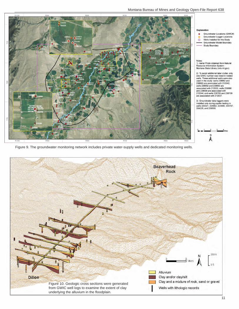
appear to be continuous in some areas and less so in others ( ig. 10). In the more continuous ar-eas, these materials may effectively form localized con ining beds separating the alluvial and Tertiary sediment aquifers; in contrast, the discontinuities allow for a direct connection between the alluvium and Tertiary sediments. Because evidence of a dis-tinct, continuous clay unit was lacking, the clay was numerically modeled as part of the Tertiary sedi-ment aquifer (see Model Grid section). Tertiary Sediment Aquifer
The Tertiary sediments (Ts, ig. 5), which un-derlie the alluvium in the loodplain and comprise most of the East and West Benches, include a wide range of lithologies. Figure 7 illustrates the over-all ine-grained nature of the sediments. Depth to water in this aquifer ranges from approximately 3 to 35 ft below ground surface in the loodplain; 13 to 127 ft on the East Bench; and 2 to 300 ft on the West Bench.
During installation of well 242403 ( ig. 9, T. 5 S., R. 7 W.) in the loodplain, indurated silt and sand were observed below 65 ft and were considered
to be the top of the Tertiary. Farther south, (well 255492, T. 6 S., R. 8 W.) the Quaternary–Tertiary contact was less distinct. Several clay layers were encountered, with the thickest being about 20 ft at 65 to 85 ft below ground surface. Below 85 ft, indu-rated silt was encountered and considered Tertiary sediments. The thickness of the Tertiary sediments beneath the loodplain is uncertain. The deepest well completed in these sediments is 460 ft deep, and it does not fully penetrate the unit.
The West Bench Tertiary sediments consist of ine to coarse sands, gravels, cemented gravels,
and interbedded clay and silt. The numerous clay and silt layers generally range from 1 to 12 ft thick. However, a 40-ft-thick silty clay (60 to 100 ft below ground surface) was identi ied during one well installation (well 254962, T. 6 S., R. 8 W.). Bedrock noted in well logs indicates that Tertiary sediments may only be about 60 ft thick in some areas of the West Bench. The deepest wells on the West Bench that are completed in Tertiary sediments are about 400 to 500 ft deep.
The East Bench Tertiary sediments are similar to the West Bench, in that the lithology consists of
Figure 8. A sedimentary bedrock outcrop, observed in August 2010, is located in the northern portion of the West Bench.
11
Montana Bureau of Mines and Geology Open-File Report 638
Figure 9. The groundwater monitoring network includes private water-supply wells and dedicated monitoring wells.
Figure 10. Geologic cross sections were generated from GWIC well logs to examine the extent of clay underlying the alluvium in the fl oodplain.
12
Butler and Abdo, 2013
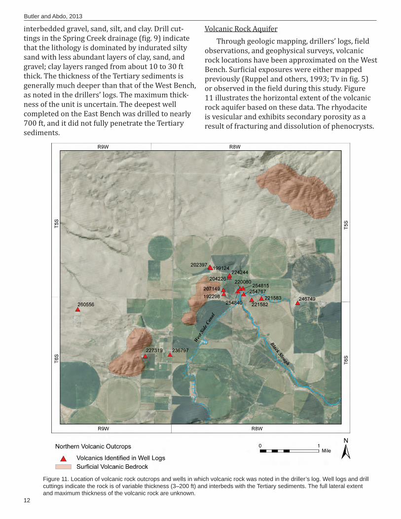
interbedded gravel, sand, silt, and clay. Drill cut-tings in the Spring Creek drainage ( ig. 9) indicate that the lithology is dominated by indurated silty sand with less abundant layers of clay, sand, and gravel; clay layers ranged from about 10 to 30 ft thick. The thickness of the Tertiary sediments is generally much deeper than that of the West Bench, as noted in the drillers’ logs. The maximum thick-ness of the unit is uncertain. The deepest well completed on the East Bench was drilled to nearly 700 ft, and it did not fully penetrate the Tertiary sediments.
Volcanic Rock AquiferThrough geologic mapping, drillers’ logs, ield
observations, and geophysical surveys, volcanic rock locations have been approximated on the West Bench. Sur icial exposures were either mapped previously (Ruppel and others, 1993; Tv in ig. 5) or observed in the ield during this study. Figure 11 illustrates the horizontal extent of the volcanic rock aquifer based on these data. The rhyodacite is vesicular and exhibits secondary porosity as a result of fracturing and dissolution of phenocrysts.
Figure 11. Location of volcanic rock outcrops and wells in which volcanic rock was noted in the driller’s log. Well logs and drill cuttings indicate the rock is of variable thickness (3–200 ft) and interbeds with the Tertiary sediments. The full lateral extent and maximum thickness of the volcanic rock are unknown.
13
Montana Bureau of Mines and Geology Open-File Report 638
The volcanic rock of the West Bench is believed to be older than or contemporaneous with the Ter-tiary sediments, and well logs indicate that it both underlies and inter ingers with the sediments. The volcanic low deposits appear to be variable in thickness, ranging from a few feet to 200 ft in well log descriptions; the maximum thickness is un-known. Depth to water in this aquifer ranges from approximately 10 to 35 ft below ground surface.
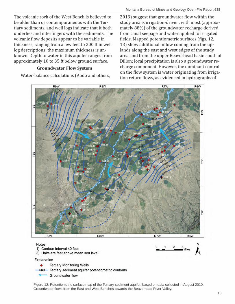
Groundwater Flow SystemWater-balance calculations (Abdo and others,
2013) suggest that groundwater low within the study area is irrigation-driven, with most (approxi-mately 88%) of the groundwater recharge derived from canal seepage and water applied to irrigated ields. Mapped potentiometric surfaces ( igs. 12,
13) show additional in low coming from the up-lands along the east and west edges of the study area, and from the upper Beaverhead basin south of Dillon; local precipitation is also a groundwater re-charge component. However, the dominant control on the low system is water originating from irriga-tion return lows, as evidenced in hydrographs of
Figure 12. Potentiometric surface map of the Tertiary sediment aquifer, based on data collected in August 2010. Groundwater fl ows from the East and West Benches towards the Beaverhead River Valley.
14
Butler and Abdo, 2013
wells within the lower Beaverhead basin’s irrigated areas ( ig.14); they show an annual pattern of a steady rise from late spring through late summer, followed by a plateau in the fall, and then a decline through early spring.
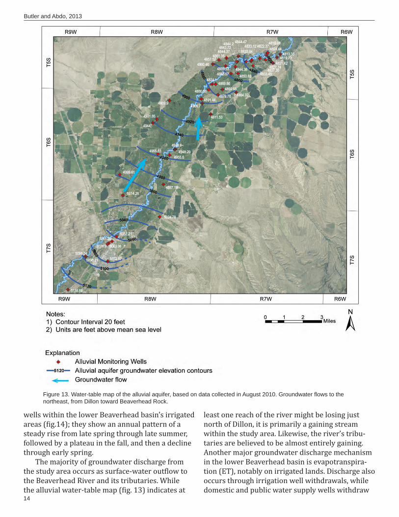
The majority of groundwater discharge from the study area occurs as surface-water out low to the Beaverhead River and its tributaries. While the alluvial water-table map ( ig. 13) indicates at
least one reach of the river might be losing just north of Dillon, it is primarily a gaining stream within the study area. Likewise, the river’s tribu-taries are believed to be almost entirely gaining. Another major groundwater discharge mechanism in the lower Beaverhead basin is evapotranspira-tion (ET), notably on irrigated lands. Discharge also occurs through irrigation well withdrawals, while domestic and public water supply wells withdraw
Figure 13. Water-table map of the alluvial aquifer, based on data collected in August 2010. Groundwater fl ows to the northeast, from Dillon toward Beaverhead Rock.

15
Montana Bureau of Mines and Geology Open-File Report 638
Figure 14. Water-level hydrographs from wells on irrigated land in the Lower Beaverhead study area. The groundwater-level fl uctuations refl ect the infl uence of irrigation recharge. Well 109060 is located in sec. 25, T. 6 S., R. 9 W., and well 259540 is located in sec. 29, T. 6 S., R. 7 W
16
Butler and Abdo, 2013
relatively small amounts (Abdo and others, 2013). Lastly, groundwater low discharges at the down-gradient pinch point of the study area, near Bea-verhead Rock; due to the shallow bedrock at this location (Geologic Framework section), most of the low is believed to move into streams and through
the shallow alluvium. Volumetric estimates of wa-ter moving through the system are provided in the Groundwater Budget section.
The three units (alluvial, Tertiary sediment, and volcanic rock aquifers) are hydrogeologically con-nected. The volcanic rock aquifer is distinct in that groundwater moves through fractures rather than porous media. However, the fractures are so ex-tensive that, when viewed at the scale of the study area, they can be treated as equivalent porous media.
Within the study area’s aquifer system, ground-water lows from the benches to the loodplain ( ig. 12). The groundwater gradient on the East Bench is about 0.01. The gradient is slightly gentler on the West Bench, about 0.009, and lattens to about 0.006 in the loodplain. The lower gradient in the
loodplain is due to the higher transmissivity and geometry of the alluvial aquifer. The slightly steep-er gradient of the East Bench vs. the West Bench could be caused by an overall higher transmissivity of the aquifers on the West Bench, the higher leak-age rate of the East Bench Canal as compared to the West Side Canal (Groundwater Budget section), and/or topographic controls.Vertical Gradients
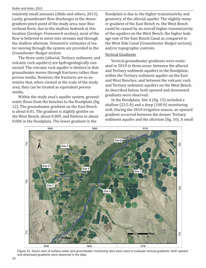
Vertical groundwater gradients were evalu-ated in 2010 in three areas: between the alluvial and Tertiary sediment aquifers in the loodplain; within the Tertiary sediment aquifer on the East and West Benches; and between the volcanic rock and Tertiary sediment aquifers on the West Bench. As described below, both upward and downward gradients were observed.
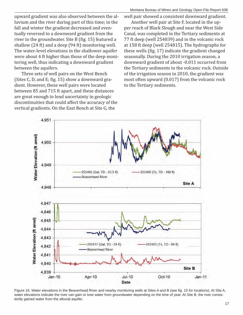
In the loodplain, Site A ( ig. 15) included a shallow (23.5 ft) and a deep (108 ft) monitoring well. During the 2010 irrigation season, an upward gradient occurred between the deeper Tertiary sediment aquifer and the alluvium ( ig. 16). A small
Figure 15. Seven sets of surface-water and groundwater monitoring sites were used to evaluate vertical gradients. Both upward and downward gradients were observed in the data.
17
Montana Bureau of Mines and Geology Open-File Report 638
upward gradient was also observed between the al-luvium and the river during part of this time; in the fall and winter the gradient decreased and even-tually reversed to a downward gradient from the river to the groundwater. Site B ( ig. 15) featured a shallow (24 ft) and a deep (94 ft) monitoring well. The water-level elevations in the shallower aquifer were about 4 ft higher than those of the deep moni-toring well, thus indicating a downward gradient between the aquifers.
Three sets of well pairs on the West Bench (Sites C, D, and E; ig. 15) show a downward gra-dient. However, these well pairs were located between 85 and 715 ft apart, and these distances are great enough to lend uncertainty in geologic discontinuities that could affect the accuracy of the vertical gradients. On the East Bench at Site G, the
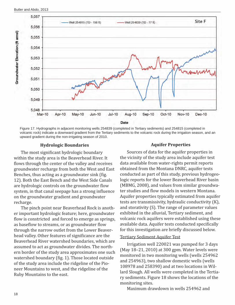
well pair showed a consistent downward gradient.Another well pair at Site F, located in the up-
per reach of Black Slough and near the West Side Canal, was completed in the Tertiary sediments at 77 ft deep (well 254839) and in the volcanic rock at 158 ft deep (well 254815). The hydrographs for these wells ( ig. 17) indicate the gradient changed seasonally. During the 2010 irrigation season, a downward gradient of about -0.011 occurred from the Tertiary sediments to the volcanic rock. Outside of the irrigation season in 2010, the gradient was most often upward (0.017) from the volcanic rock to the Tertiary sediments.
Figure 16. Water elevations in the Beaverhead River and nearby monitoring wells at Sites A and B (see fi g. 15 for locations). At Site A, water elevations indicate the river can gain or lose water from groundwater depending on the time of year. At Site B, the river consis-tently gained water from the alluvial aquifer.
18
Butler and Abdo, 2013
Hydrologic BoundariesThe most signi icant hydrologic boundary
within the study area is the Beaverhead River. It lows through the center of the valley and receives
groundwater recharge from both the West and East Benches, thus acting as a groundwater sink ( ig. 12). Both the East Bench and the West Side Canals are hydrologic controls on the groundwater low system, in that canal seepage has a strong in luence on the groundwater gradient and groundwater recharge.
The pinch point near Beaverhead Rock is anoth-er important hydrologic feature; here, groundwater low is constricted and forced to emerge as springs,
as base low to streams, or as groundwater low through the narrow outlet from the Lower Beaver-head valley. Other features of signi icance are the Beaverhead River watershed boundaries, which are assumed to act as groundwater divides. The north-ern border of the study area approximates one such watershed boundary ( ig. 1). Those located outside of the study area include the ridgeline of the Pio-neer Mountains to west, and the ridgeline of the Ruby Mountains to the east.
Aquifer PropertiesSources of data for the aquifer properties in
the vicinity of the study area include aquifer test data available from water-rights permit reports obtained from the Montana DNRC, aquifer tests conducted as part of this study, previous hydrogeo-logic reports for the lower Beaverhead River basin (MBMG, 2008), and values from similar groundwa-ter studies and low models in western Montana. Aquifer properties typically estimated from aquifer tests are transmissivity, hydraulic conductivity (K), and storativity (S). The range of parameter values exhibited in the alluvial, Tertiary sediment, and volcanic rock aquifers were established using these available data. Aquifer tests conducted speci ically for this investigation are brie ly discussed below. Tertiary Sediment Aquifer Test
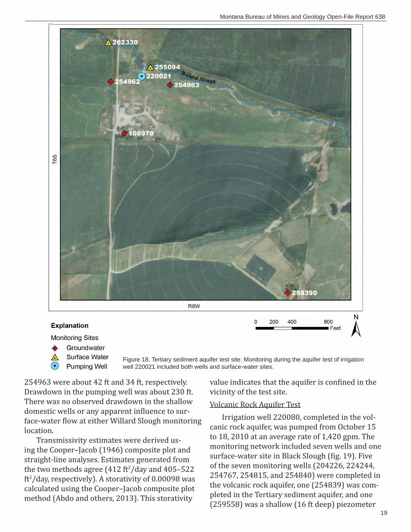
Irrigation well 220021 was pumped for 3 days (May 18–21, 2010) at 300 gpm. Water levels were monitored in two monitoring wells (wells 254962 and 254963), two shallow domestic wells (wells 108978 and 258390) and at two locations in Wil-lard Slough. All wells were completed in the Tertia-ry sediments. Figure 18 shows the locations of the monitoring sites.
Maximum drawdown in wells 254962 and
Figure 17. Hydrographs in adjacent monitoring wells 254839 (completed in Tertiary sediments) and 254815 (completed in volcanic rock) indicate a downward gradient from the Tertiary sediments to the volcanic rock during the irrigation season, and an upward gradient during the non-irrigating season of 2010.
19
Montana Bureau of Mines and Geology Open-File Report 638
254963 were about 42 ft and 34 ft, respectively. Drawdown in the pumping well was about 230 ft. There was no observed drawdown in the shallow domestic wells or any apparent in luence to sur-face-water low at either Willard Slough monitoring location.
Transmissivity estimates were derived us-ing the Cooper–Jacob (1946) composite plot and straight-line analyses. Estimates generated from the two methods agree (412 ft2/day and 405–522 ft2/day, respectively). A storativity of 0.00098 was calculated using the Cooper–Jacob composite plot method (Abdo and others, 2013). This storativity
value indicates that the aquifer is con ined in the vicinity of the test site.Volcanic Rock Aquifer Test
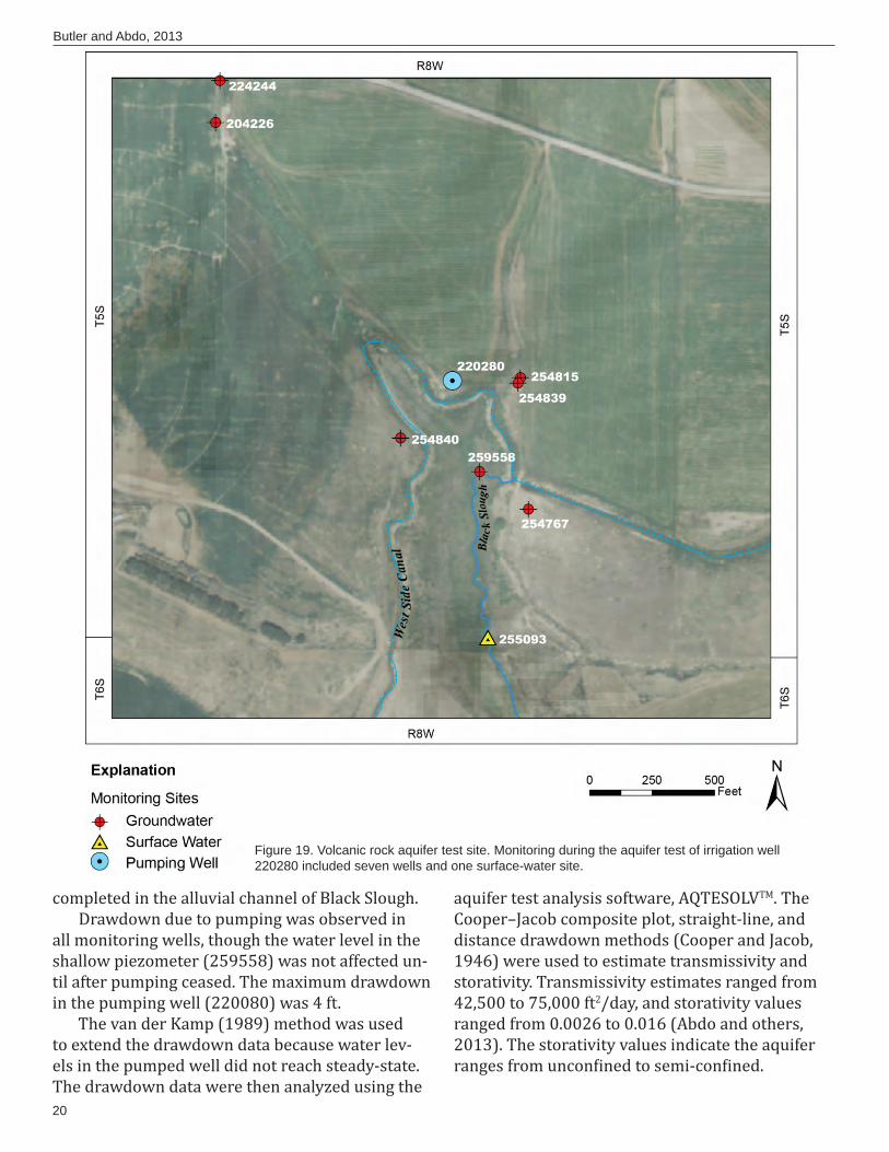
Irrigation well 220080, completed in the vol-canic rock aquifer, was pumped from October 15 to 18, 2010 at an average rate of 1,420 gpm. The monitoring network included seven wells and one surface-water site in Black Slough ( ig. 19). Five of the seven monitoring wells (204226, 224244, 254767, 254815, and 254840) were completed in the volcanic rock aquifer, one (254839) was com-pleted in the Tertiary sediment aquifer, and one (259558) was a shallow (16 ft deep) piezometer
Figure 18. Tertiary sediment aquifer test site. Monitoring during the aquifer test of irrigation well 220021 included both wells and surface-water sites.
20
Butler and Abdo, 2013
completed in the alluvial channel of Black Slough. Drawdown due to pumping was observed in
all monitoring wells, though the water level in the shallow piezometer (259558) was not affected un-til after pumping ceased. The maximum drawdown in the pumping well (220080) was 4 ft. The van der Kamp (1989) method was used
to extend the drawdown data because water lev-els in the pumped well did not reach steady-state. The drawdown data were then analyzed using the
aquifer test analysis software, AQTESOLVTM. The Cooper–Jacob composite plot, straight-line, and distance drawdown methods (Cooper and Jacob, 1946) were used to estimate transmissivity and storativity. Transmissivity estimates ranged from 42,500 to 75,000 ft2/day, and storativity values ranged from 0.0026 to 0.016 (Abdo and others, 2013). The storativity values indicate the aquifer ranges from uncon ined to semi-con ined.
Figure 19. Volcanic rock aquifer test site. Monitoring during the aquifer test of irrigation well 220280 included seven wells and one surface-water site.
21
Montana Bureau of Mines and Geology Open-File Report 638
Alluvial Aquifer TestsWhile tests were not conducted within the allu-
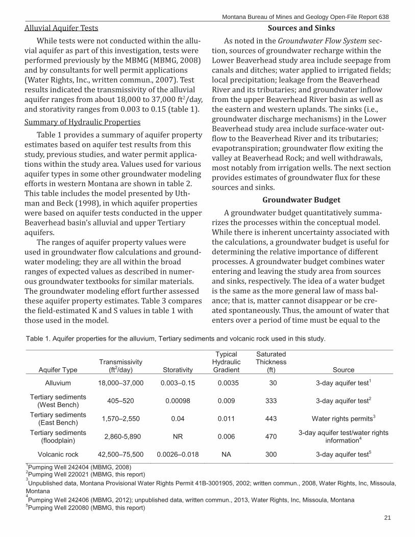
vial aquifer as part of this investigation, tests were performed previously by the MBMG (MBMG, 2008) and by consultants for well permit applications (Water Rights, Inc., written commun., 2007). Test results indicated the transmissivity of the alluvial aquifer ranges from about 18,000 to 37,000 ft2/day, and storativity ranges from 0.003 to 0.15 (table 1). Summary of Hydraulic Properties
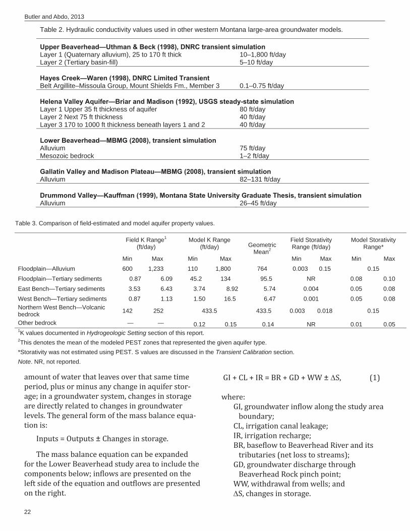
Table 1 provides a summary of aquifer property estimates based on aquifer test results from this study, previous studies, and water permit applica-tions within the study area. Values used for various aquifer types in some other groundwater modeling efforts in western Montana are shown in table 2. This table includes the model presented by Uth-man and Beck (1998), in which aquifer properties were based on aquifer tests conducted in the upper Beaverhead basin’s alluvial and upper Tertiary aquifers.
The ranges of aquifer property values were used in groundwater low calculations and ground-water modeling; they are all within the broad ranges of expected values as described in numer-ous groundwater textbooks for similar materials. The groundwater modeling effort further assessed these aquifer property estimates. Table 3 compares the ield-estimated K and S values in table 1 with those used in the model.
Sources and SinksAs noted in the Groundwater Flow System sec-
tion, sources of groundwater recharge within the Lower Beaverhead study area include seepage from canals and ditches; water applied to irrigated ields; local precipitation; leakage from the Beaverhead River and its tributaries; and groundwater in low from the upper Beaverhead River basin as well as the eastern and western uplands. The sinks (i.e., groundwater discharge mechanisms) in the Lower Beaverhead study area include surface-water out-low to the Beaverhead River and its tributaries;
evapotranspiration; groundwater low exiting the valley at Beaverhead Rock; and well withdrawals, most notably from irrigation wells. The next section provides estimates of groundwater lux for these sources and sinks.
Groundwater BudgetA groundwater budget quantitatively summa-
rizes the processes within the conceptual model. While there is inherent uncertainty associated with the calculations, a groundwater budget is useful for determining the relative importance of different processes. A groundwater budget combines water entering and leaving the study area from sources and sinks, respectively. The idea of a water budget is the same as the more general law of mass bal-ance; that is, matter cannot disappear or be cre-ated spontaneously. Thus, the amount of water that enters over a period of time must be equal to the
22
Butler and Abdo, 2013
amount of water that leaves over that same time period, plus or minus any change in aquifer stor-age; in a groundwater system, changes in storage are directly related to changes in groundwater levels. The general form of the mass balance equa-tion is:
Inputs = Outputs ± Changes in storage.
The mass balance equation can be expanded for the Lower Beaverhead study area to include the components below; in lows are presented on the left side of the equation and out lows are presented on the right.
GI + CL + IR = BR + GD + WW ± S, (1)
where: GI, groundwater in low along the study area boundary;
CL, irrigation canal leakage; IR, irrigation recharge; BR, base low to Beaverhead River and its
tributaries (net loss to streams); GD, groundwater discharge through
Beaverhead Rock pinch point; WW, withdrawal from wells; and S, changes in storage.
Table 2. Hydraulic conductivity values used in other western Montana large-area groundwater models.
Layer 1 (Quaternary alluvium), 25 to 170 ft thick 10–1,800 ft/day Layer 2 (Tertiary basin-fill) 5–10 ft/day
Belt Argillite–Missoula Group, Mount Shields Fm., Member 3 0.1–0.75 ft/day
Layer 1 Upper 35 ft thickness of aquifer 80 ft/day Layer 2 Next 75 ft thickness 40 ft/day Layer 3 170 to 1000 ft thickness beneath layers 1 and 2 40 ft/day
Alluvium 75 ft/dayMesozoic bedrock 1–2 ft/day
Alluvium 82–131 ft/day
Alluvium 26–45 ft/day
Table 3. Comparison of field-estimated and model aquifer property values.
Field K Range1
(ft/day)Model K Range
(ft/day) Geometric Mean2
Field Storativity Range (ft/day)
Model Storativity Range*
Min Max Min Max Min Max Min Max Floodplain—Alluvium 600 1,233 110 1,800 764 0.003 0.15 0.15 Floodplain—Tertiary sediments 0.87 6.09 45.2 134 95.5 NR 0.08 0.10 East Bench—Tertiary sediments 3.53 6.43 3.74 8.92 5.74 0.004 0.05 0.08 West Bench—Tertiary sediments 0.87 1.13 1.50 16.5 6.47 0.001 0.05 0.08 Northern West Bench—Volcanic bedrock 142 252 433.5 433.5 0.003 0.018 0.15
Other bedrock — — 0.12 0.15 0.14 NR 0.01 0.05 1K values documented in Hydrogeologic Setting section of this report. 2This denotes the mean of the modeled PEST zones that represented the given aquifer type. *Storativity was not estimated using PEST. S values are discussed in the Transient Calibration section. Note. NR, not reported.
23
Montana Bureau of Mines and Geology Open-File Report 638
These components were based on the study area hydrogeology and land uses that affect groundwa-ter. Certain components re lect the net result of a combination of sub components. For instance, the irrigation recharge component accounts for both precipitation and evapotranspiration on irrigated lands. The following discussion summarizes the water budget components used in the model as shown in equation 1. All component estimates have inherent uncertainty, some to a greater degree than others. For this reason the model components were not calibrated precisely to ield estimates; rather, the ield estimates were used as guides to which the model components were approximated.
Groundwater in low (GI) enters the study area from upgradient areas along the East Bench, West Bench, and in the loodplain at Dillon (i.e., the upgradient border of the Lower Beaverhead Val-ley). Along the study area’s East Bench boundary, groundwater moves through the Tertiary sediment aquifer, which is relatively thick and continuous. In contrast, in low from the West Bench bound-ary is derived from the Tertiary sediment aquifer as well as sedimentary rock and volcanic rock ( ig. 5); the bedrock aquifers are believed to provide less recharge due to their relatively low hydraulic conductivity values. Along the study area boundary in the loodplain, groundwater lows from the Up-per Beaverhead Valley into the Lower Beaverhead Valley; the majority of in low is derived from the highly transmissive alluvial aquifer, while a smaller amount enters through the underlying Tertiary sed-iment aquifer. The estimate of groundwater enter-ing the site was calculated using groundwater low nets and Darcy’s law:
Q = KiA, (2)where: Q, groundwater low;
K, hydraulic conductivity; i, hydraulic gradient; and A, low tube area (tube width multiplied by saturated aquifer thickness).
Using this approach, groundwater in low from the study-area boundaries was calculated. About 142 acre-ft/yr and 3,161 acre-ft/yr were estimated to low in from the boundaries of the West Bench and
East Bench, respectively. Approximately 2,765 acre-ft/yr was estimated to low into the model from the alluvium and underlying Tertiary sediment aquifer
at the south edge of the model. The total in low from boundaries was an estimated 6,068 acre-ft/yr.
Leakage from irrigation canals (CL) provides a source of recharge to the groundwater. GIS analysis of canals showed that 12.6 miles of the East Bench Canal and 14.3 miles of the West Side Canal are present in the modeled portion of the study area. Leakage is quite evident in several hydrographs ( ig. 14). During the summer of 2010, a series of low measurements were made along each canal,
and diversion records for each day of the low measurements were obtained. Based on these data, seepage rates were estimated for several reaches of each canal, and an average value per canal was cal-culated (Abdo and others, 2013). The average seep-age rates used as initial model inputs for the East Bench Canal and West Side Canal were 2.8 cfs/mile and 1.1 cfs/mile, respectively. Using this approach, a total of 18,100 acre-ft/year was estimated to in il-trate from the canals during the irrigation season.
When water (irrigation water plus precipita-tion) is applied to a ield in excess of crop demand and evaporation, the excess must either runoff or in iltrate to the subsurface. On irrigated ields, the water that recharges groundwater is termed irriga-tion recharge (IR). A linear groundwater recharge rate was calculated for the irrigated land within the study area as follows:
Recharge Rate = Pin + Rirr, (3)
where Pin is total precipitation and Rirr is the groundwater recharge from irrigation, which was calculated by the NRCS IWR method (appendix B). The IWR method considers the recharge rates for three irrigation types: lood, pivot, and sprinkler. In non-irrigated areas, groundwater recharge from precipitation was assumed to be negligible. Using this approach, the irrigation recharge was calcu-lated to be approximately 14,000 acre-ft/yr on the West Bench, 16,000 acre-ft/yr on the East Bench, and 18,000 acre-ft/yr in the loodplain, for a total of 48,000 acre-ft/yr.
Base low to the Beaverhead River and its tribu-taries (BR) is the primary means by which ground-water exits the aquifers of the Lower Beaverhead study area. Although ield data (e.g., stage, low, and alluvial groundwater-level measurements) show that the Beaverhead River loses low to the alluvial aquifer in certain reaches, it is generally a gaining stream. To estimate base low to the river, surface-
24
Butler and Abdo, 2013
water out lows were subtracted from surface-water in lows. The in lows consisted of the Beaverhead River at Dillon and its tributaries that originate from outside the study area and join the river with-in the study area, including Blacktail Deer Creek and Stone Creek. Surface-water out lows consisted of only the river at Beaverhead Rock. The resulting base low within the study area was estimated to be between 25,000 and 35,000 acre-ft/yr. This esti-mate was of a range rather than a single value due to the inherent uncertainty in the approach.
In the Lower Beaverhead study area, ground-water discharges through the pinch point at Bea-verhead Rock ( ig. 2). Groundwater discharge (GD) was estimated using Darcy’s Law, as with the groundwater in low component. Because water well logs indicate that bedrock underlies the allu-vium at the pinch point, most of the groundwater likely lows through the alluvium. Using Darcy’s Law, the alluvial aquifer thickness in this location was approximated to be 30 ft and was assigned a K of 1,200 ft/day; the underlying bedrock had a thick-ness of 470 ft in the model and was assigned a K of 0.1 ft. The valley width was measured using aerial photography and is about 1,000 ft wide at this loca-tion. Last, the groundwater gradient was estimated from potentiometric maps ( igs. 12,13). The result-ing discharge estimate was about 1,500 acre-ft/yr.
Well withdrawals (WW) are another groundwa-ter sink in the Lower Beaverhead study area. Only irrigation wells and public water supply (PWS) wells were simulated in the model; withdrawals from domestic wells were not considered due to their relatively low water usage. The number of such wells within the study area was estimated by inventorying irrigation and PWS wells through the GWIC database. Water-rights records and permit applications were also inventoried through the DNRC Water Rights Bureau and through consul-tants who produced hydrogeologic reports for Dillon-area well permit applications (PBS&J, writ-ten commun., 2005; WET, written commun., 2004; Water Rights, Inc., written commun., 2007); these records were reviewed for such data as crop acre-age, crop type, and water use allotments. An annual withdrawal volume was then calculated for each well based on this information as well as the IWR per-acre crop requirements (appendix B). Sum-mertime aerial photos and transducer data (where available) were also used to verify well use. Further
detail on this approach is provided in appendix C. The resulting well withdrawal estimate was ap-proximately 8,150 acre-ft/yr.
Annual water budgets often ind a balance between the amount of water that enters and exits the study area; however, changes in storage (S) in the aquifer system can cause the volumes of in low and out low to differ. 2010 was the 23rd wettest year in the past 111 years of recorded precipita-tion in the Dillon area. Examination of groundwater hydrographs revealed a gain in storage within the study area in 2010. The volume of the change in storage was estimated by comparing water levels from January 2010 and January 2011 for the West Bench, East Bench, and loodplain areas. An aver-age change in groundwater level was calculated from numerous wells within each of the areas. The average water-level change was then multiplied by the estimated effective porosity for each area and by the total acreage. The resulting estimate of groundwater held in storage during 2010 was about 17,000 acre-ft. Most of this increase in stored groundwater occurred on the East Bench (72%; Abdo and others, 2013).
The model water budget results in both the steady-state and transient versions of the model are presented in the Calibration section because certain budget components were adjusted during calibration. Results showed that irrigation (i.e., canal leakage and applied irrigation water) was the predominant source of recharge to the model, which demonstrates its considerable in luence on groundwater low within the Lower Beaverhead study area. The primary means of groundwater dis-charge from the model was base low to the Beaver-head River and its tributaries.
COMPUTER CODEGroundwater Modeling Systems (GMS) software
was used to develop a MODFLOW-2000 groundwa-ter low model (Aquaveo, 2010). MODFLOW-2000 is a widely accepted groundwater low program developed by the US Geological Survey (Harbaugh and others, 2000). It simulates groundwater low numerically using a inite-difference method. The version of GMS used for this modeling was GMS 7.1.2, with a build date of April 16, 2010. The ver-sion of MODFLOW-2000 operated in GMS 7.1.2 was Version 1.18.01, compiled June 20, 2008.
25
Montana Bureau of Mines and Geology Open-File Report 638
PEST is a general purpose parameter estimation utility developed by John Doherty of Watermark Numerical Computing (Doherty, 2010). PEST was used for automated parameter estimation in cer-tain model runs. The version of PEST operated in GMS 7.1.2 was PEST Version 12.0.
GROUNDWATER FLOW MODEL CONSTRUCTION
Model GridThe GMS project was operated using the North
American Datum (NAD) 1983 Montana State Plane coordinates, with vertical units of U.S. Survey Feet. The model grid was created using a uniform grid frame with an X origin of 1,140,727 ft, Y origin of 359,905 ft, and Z origin of 4700 ft. Lengths of the
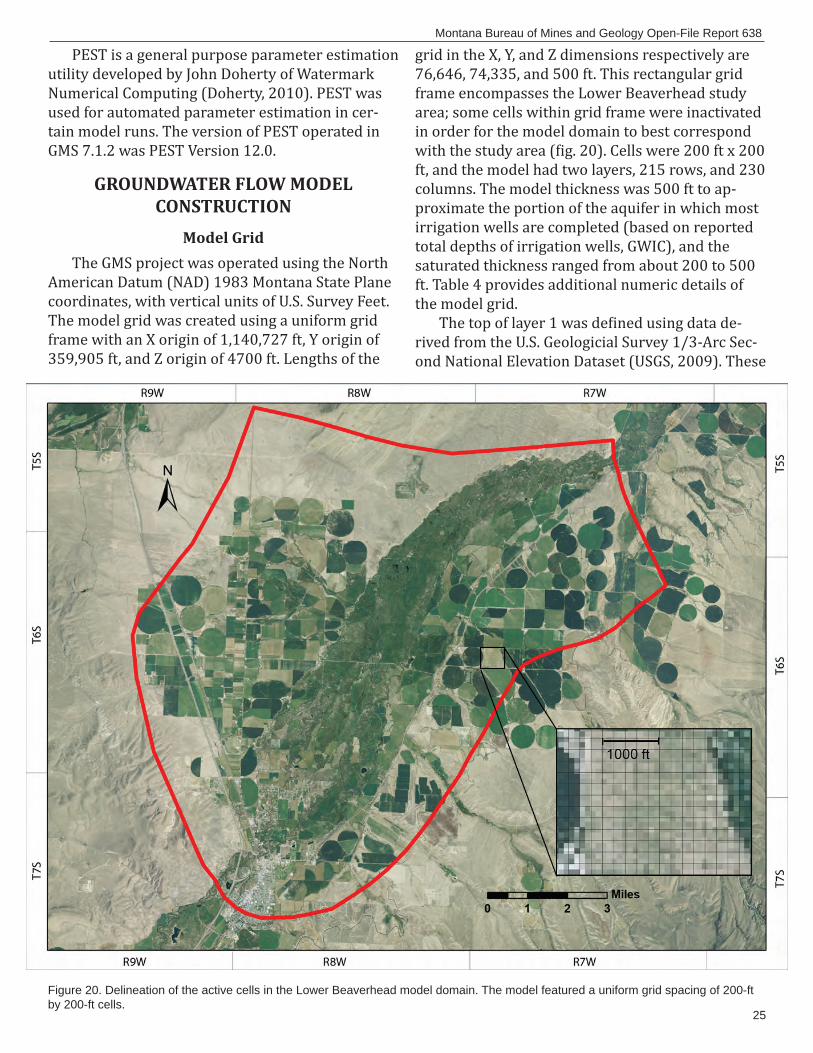
grid in the X, Y, and Z dimensions respectively are 76,646, 74,335, and 500 ft. This rectangular grid frame encompasses the Lower Beaverhead study area; some cells within grid frame were inactivated in order for the model domain to best correspond with the study area ( ig. 20). Cells were 200 ft x 200 ft, and the model had two layers, 215 rows, and 230 columns. The model thickness was 500 ft to ap-proximate the portion of the aquifer in which most irrigation wells are completed (based on reported total depths of irrigation wells, GWIC), and the saturated thickness ranged from about 200 to 500 ft. Table 4 provides additional numeric details of the model grid.
The top of layer 1 was de ined using data de-rived from the U.S. Geologicial Survey 1/3-Arc Sec-ond National Elevation Dataset (USGS, 2009). These
Figure 20. Delineation of the active cells in the Lower Beaverhead model domain. The model featured a uniform grid spacing of 200-ft by 200-ft cells.
26
Butler and Abdo, 2013
data were converted into a scatter point dataset and imported into GMS as a text ile. This scatter point set is referred to here as the Digital Elevation Model (DEM) scatter point set. The DEM scatter point spacing is about 186 ft, which is similar to the cell size of 200 ft. The bottom of layer 1 was de-ined by a surface derived from two elements. The irst element was a surface de ined by subtracting
30 ft from the elevation of the DEM scatter point set. This irst approach was used in the loodplain, where the upper 30 ft of the grid approximated the alluvial aquifer. The second element was a compos-ite of lat surfaces that changed elevation westward and eastward from the loodplain onto the benches. The shifts in elevation of the bottom surface cor-respond with large shifts in elevation of the top surface (i.e., the land surface). Layer 1 was about 250 ft thick toward the eastern and western extents of the grid, where the model represents the Tertia-ry sediments and volcanic bedrock. This thickness ensured that the maximum depth to groundwater would remain above the bottom of layer 1 and prevent cells from drying ( ig. 21). In the lood-plain, layer 2 represented the Tertiary sediments underlying the alluvium; as with layer 1, layer 2 represented the Tertiary sediments on the East Bench and a combination of Tertiary sediments and volcanic bedrock on the West Bench. Because the model thickness was held constant (500 ft), the
Table 4. Details of the model grid as listed in GMS.Grid Type Cell CenteredX origin (ft) 1,140,727Y origin (ft) 359,905Z origin (ft) 4,700Length in X (ft) 76,646Length in Y (ft) 74,335Length in Z (ft) 500Rotation angle 0°Minimum scalar 4,827Maximum scalar 5,155Number of rows (i) 372Number of columns (j) 383Number of layers (k) 2Number of nodes 358,080Number of cells 284,952Number of active cells 146,635Number of inactive cells 138,317
Figu
re 2
1. M
odel
cro
ss s
ectio
n th
roug
h R
ow 2
37, w
hich
runs
in a
Wes
t–E
ast o
rient
atio
n in
the
mod
el g
rid. T
he g
rid h
as a
uni
form
thic
knes
s of
500
ft a
nd fe
atur
es
two
laye
rs, w
ith th
e up
per l
ayer
repr
esen
ting
the
allu
vium
with
in th
e fl o
odpl
ain.

27
Montana Bureau of Mines and Geology Open-File Report 638
thickness of layer 2 was variable; it was relatively thick in the loodplain (approximately 470 ft) and thinner at the east and west edges of the benches (approximately 250 ft).
Prior to arriving at this layer con iguration, another version was tested. The initial version of the model grid tightly discretized the vertical hydrogeology vertically using four layers. The goal of the four-layer design was to reproduce site-scale observations in the volcanic rock aquifer on the northern West Bench (Aquifer Properties section). However, the degree of detail could not be ad-equately calibrated via PEST due to a lack of cali-bration targets within certain layers (Steady-State Calibration section).
Hydraulic ParametersPrior to model calibration, K and S values were
assigned to polygonal zones in the model based on the aquifer property estimates from aquifer tests performed during this investigation and previous investigations (Aquifer Properties section). The polygon extents were based on the hydrogeologic units of the conceptual model (Geologic Framework section); the units included the loodplain alluvium, the volcanic rock on the West Bench, and the Ter-tiary sediments. The initial K values were modi ied during the steady-state model calibration process.
Storativity was introduced in the transient mod-el. Values were assigned in polygonal zones based on estimates presented in the Hydrogeologic Setting section. The simulation was divided into monthly increments to best simulate seasonal changes and to use the available monthly water-level datasets in model calibration. During the transient model cali-bration, parameter values were adjusted to render the observed water-level luctuations.
Boundary ConditionsThe boundary conditions of a numerical
groundwater model are assigned to all of the three-dimensional boundary surfaces of the aquifer system and to internal sources and sinks (ASTM, 2004). Boundary conditions represent the sources of recharge and discharge to the groundwater low system, and/or the hydraulic head at the edges of the modeled domain.
The boundary conditions for the Lower Beaver-head model follow those discussed in the Hydrolog-ic Boundaries, Sources and Sinks, and Groundwater Budget sections of this report. They can be grouped
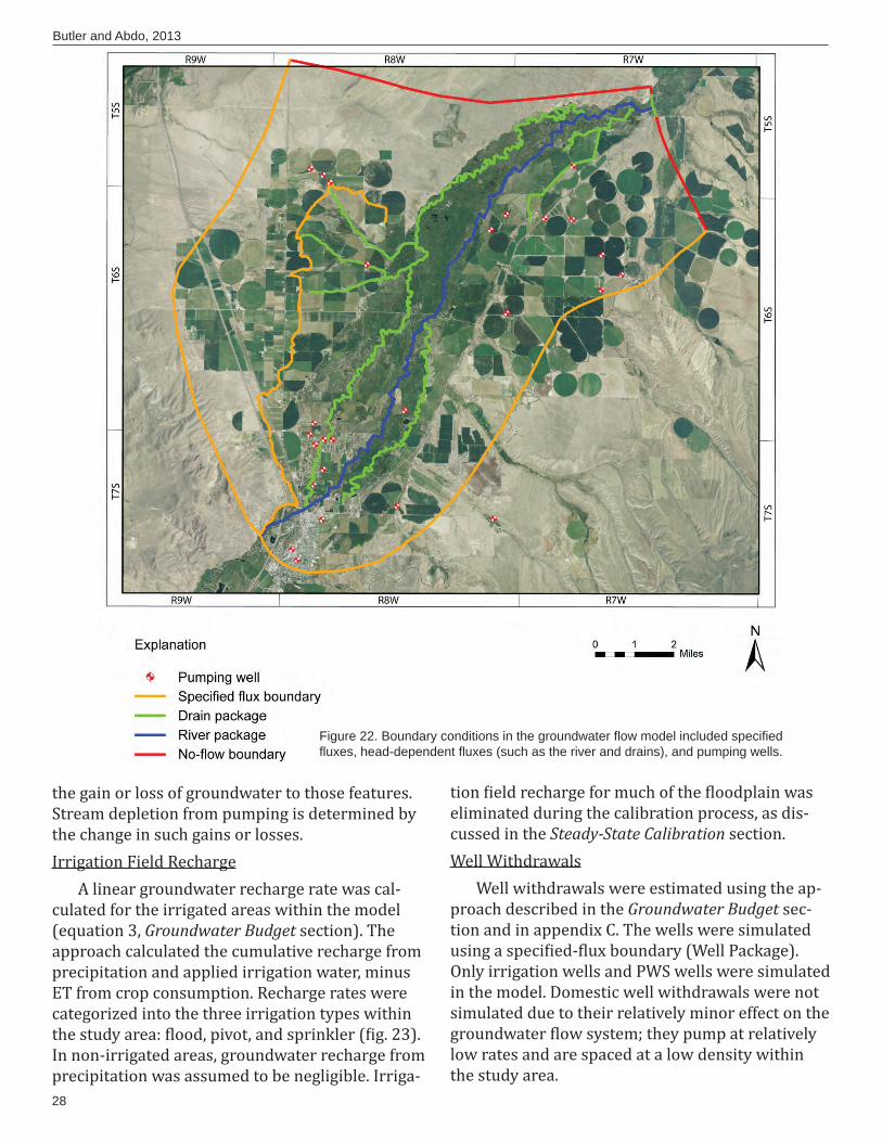
into four general categories: the model borders, surface-water bodies, aerial recharge (precipitation and applied irrigation water), and well withdraw-als. Figure 22 shows the boundary conditions in the model with the exception of aerial recharge, which is shown in igure 23. Model Borders
Speci ied- lux boundaries were used to repre-sent in low along the East and West Benches, and from the upper Beaverhead River basin into Dil-lon from the south. These boundaries were placed along contours based on the potentiometric surface map developed for this study, and they replicate the relatively stable groundwater setting observed in these areas. A speci ied- lux boundary simulates water in low or out low to the aquifer system as a user-de ined volumetric rate. Flux values were estimated using a low net approach (Groundwater Budget section), with hydraulic conductivity (K) and gradient values based on aquifer property es-timates. Along the East Bench border, the lux rate represented seepage from the East Bench Canal in addition to the upland in low component, as the canal was located just outside of the model domain.
At the portion of the model border near Beaver-head Rock, the loodplain constricts as groundwa-ter low exits the model domain. The Drain Package was assigned to this model border. This MODFLOW package allows groundwater low to exit the mod-eled aquifer. No- low boundaries were set along groundwater low lines at the remainder of the north and northeast model border; these no- low boundaries run parallel to groundwater low lines on the potentiometric surface map. Surface-Water Bodies
A speci ied- lux boundary was used to repre-sent seepage from the West Side Canal; the lux rate was based on the average rate obtained from two 2010 canal seepage runs (Abdo and others, 2013). Because the Beaverhead River both contributes (re-charges) water and drains (discharges) water from the aquifer system, the MODFLOW River Package was used; this package allows groundwater low to enter as well as exit the model. The larger sloughs within the study area are believed to only drain water from the aquifer system, and were simulated as drains. It should be noted that the River Package and Drain Package of MODFLOW do not calculate stream discharge; the modules are used to calculate
28
Butler and Abdo, 2013
the gain or loss of groundwater to those features. Stream depletion from pumping is determined by the change in such gains or losses. Irrigation Field Recharge
A linear groundwater recharge rate was cal-culated for the irrigated areas within the model (equation 3, Groundwater Budget section). The approach calculated the cumulative recharge from precipitation and applied irrigation water, minus ET from crop consumption. Recharge rates were categorized into the three irrigation types within the study area: lood, pivot, and sprinkler ( ig. 23). In non-irrigated areas, groundwater recharge from precipitation was assumed to be negligible. Irriga-
tion ield recharge for much of the loodplain was eliminated during the calibration process, as dis-cussed in the Steady-State Calibration section.Well Withdrawals
Well withdrawals were estimated using the ap-proach described in the Groundwater Budget sec-tion and in appendix C. The wells were simulated using a speci ied- lux boundary (Well Package). Only irrigation wells and PWS wells were simulated in the model. Domestic well withdrawals were not simulated due to their relatively minor effect on the groundwater low system; they pump at relatively low rates and are spaced at a low density within the study area.
Figure 22. Boundary conditions in the groundwater fl ow model included specifi ed fl uxes, head-dependent fl uxes (such as the river and drains), and pumping wells.
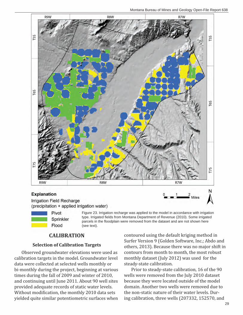
29
Montana Bureau of Mines and Geology Open-File Report 638
CALIBRATIONSelection of Calibration Targets
Observed groundwater elevations were used as calibration targets in the model. Groundwater level data were collected at selected wells monthly or bi-monthly during the project, beginning at various times during the fall of 2009 and winter of 2010, and continuing until June 2011. About 90 well sites provided adequate records of static water levels. Without modi ication, the monthly 2010 data sets yielded quite similar potentiometric surfaces when
contoured using the default kriging method in Surfer Version 9 (Golden Software, Inc.; Abdo and others, 2013). Because there was no major shift in contours from month to month, the most robust monthly dataset (July 2012) was used for the steady-state calibration.
Prior to steady-state calibration, 16 of the 90 wells were removed from the July 2010 dataset because they were located outside of the model domain. Another two wells were removed due to the non-static nature of their water levels. Dur-ing calibration, three wells (207332, 152570, and
Figure 23. Irrigation recharge was applied to the model in accordance with irrigation type. Irrigated fi elds from Montana Department of Revenue (2010). Some irrigated parcels in the fl oodplain were removed from the dataset and are not shown here (see text).
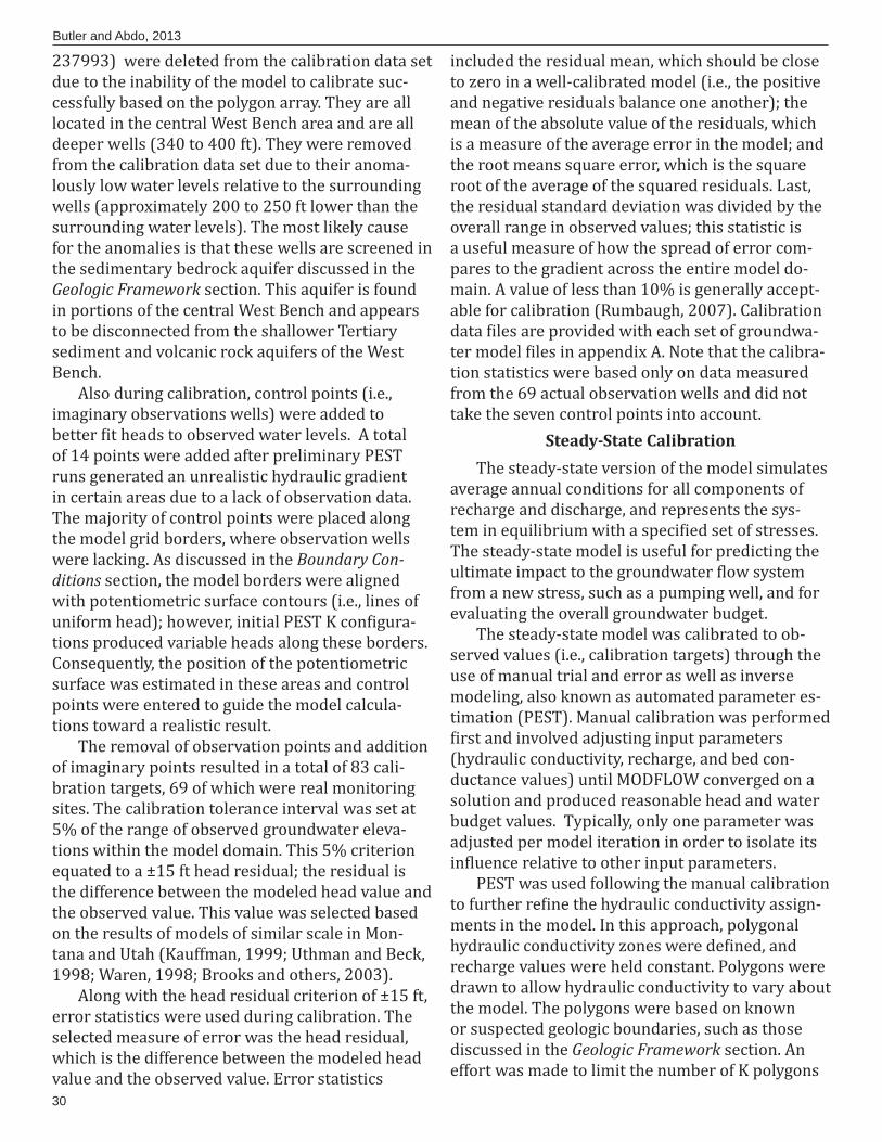
30
Butler and Abdo, 2013
237993) were deleted from the calibration data set due to the inability of the model to calibrate suc-cessfully based on the polygon array. They are all located in the central West Bench area and are all deeper wells (340 to 400 ft). They were removed from the calibration data set due to their anoma-lously low water levels relative to the surrounding wells (approximately 200 to 250 ft lower than the surrounding water levels). The most likely cause for the anomalies is that these wells are screened in the sedimentary bedrock aquifer discussed in the Geologic Framework section. This aquifer is found in portions of the central West Bench and appears to be disconnected from the shallower Tertiary sediment and volcanic rock aquifers of the West Bench.
Also during calibration, control points (i.e., imaginary observations wells) were added to better it heads to observed water levels. A total of 14 points were added after preliminary PEST runs generated an unrealistic hydraulic gradient in certain areas due to a lack of observation data. The majority of control points were placed along the model grid borders, where observation wells were lacking. As discussed in the Boundary Con-ditions section, the model borders were aligned with potentiometric surface contours (i.e., lines of uniform head); however, initial PEST K con igura-tions produced variable heads along these borders. Consequently, the position of the potentiometric surface was estimated in these areas and control points were entered to guide the model calcula-tions toward a realistic result.
The removal of observation points and addition of imaginary points resulted in a total of 83 cali-bration targets, 69 of which were real monitoring sites. The calibration tolerance interval was set at 5% of the range of observed groundwater eleva-tions within the model domain. This 5% criterion equated to a ±15 ft head residual; the residual is the difference between the modeled head value and the observed value. This value was selected based on the results of models of similar scale in Mon-tana and Utah (Kauffman, 1999; Uthman and Beck, 1998; Waren, 1998; Brooks and others, 2003).
Along with the head residual criterion of ±15 ft, error statistics were used during calibration. The selected measure of error was the head residual, which is the difference between the modeled head value and the observed value. Error statistics
included the residual mean, which should be close to zero in a well-calibrated model (i.e., the positive and negative residuals balance one another); the mean of the absolute value of the residuals, which is a measure of the average error in the model; and the root means square error, which is the square root of the average of the squared residuals. Last, the residual standard deviation was divided by the overall range in observed values; this statistic is a useful measure of how the spread of error com-pares to the gradient across the entire model do-main. A value of less than 10% is generally accept-able for calibration (Rumbaugh, 2007). Calibration data iles are provided with each set of groundwa-ter model iles in appendix A. Note that the calibra-tion statistics were based only on data measured from the 69 actual observation wells and did not take the seven control points into account.
Steady-State CalibrationThe steady-state version of the model simulates
average annual conditions for all components of recharge and discharge, and represents the sys-tem in equilibrium with a speci ied set of stresses. The steady-state model is useful for predicting the ultimate impact to the groundwater low system from a new stress, such as a pumping well, and for evaluating the overall groundwater budget.
The steady-state model was calibrated to ob-served values (i.e., calibration targets) through the use of manual trial and error as well as inverse modeling, also known as automated parameter es-timation (PEST). Manual calibration was performed irst and involved adjusting input parameters
(hydraulic conductivity, recharge, and bed con-ductance values) until MODFLOW converged on a solution and produced reasonable head and water budget values. Typically, only one parameter was adjusted per model iteration in order to isolate its in luence relative to other input parameters.
PEST was used following the manual calibration to further re ine the hydraulic conductivity assign-ments in the model. In this approach, polygonal hydraulic conductivity zones were de ined, and recharge values were held constant. Polygons were drawn to allow hydraulic conductivity to vary about the model. The polygons were based on known or suspected geologic boundaries, such as those discussed in the Geologic Framework section. An effort was made to limit the number of K polygons
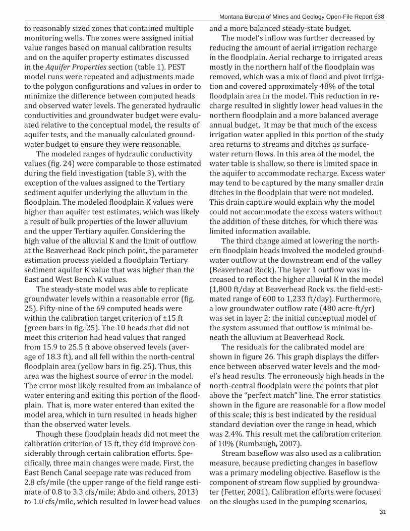
31
Montana Bureau of Mines and Geology Open-File Report 638
to reasonably sized zones that contained multiple monitoring wells. The zones were assigned initial value ranges based on manual calibration results and on the aquifer property estimates discussed in the Aquifer Properties section (table 1). PEST model runs were repeated and adjustments made to the polygon con igurations and values in order to minimize the difference between computed heads and observed water levels. The generated hydraulic conductivities and groundwater budget were evalu-ated relative to the conceptual model, the results of aquifer tests, and the manually calculated ground-water budget to ensure they were reasonable.
The modeled ranges of hydraulic conductivity values ( ig. 24) were comparable to those estimated during the ield investigation (table 3), with the exception of the values assigned to the Tertiary sediment aquifer underlying the alluvium in the loodplain. The modeled loodplain K values were
higher than aquifer test estimates, which was likely a result of bulk properties of the lower alluvium and the upper Tertiary aquifer. Considering the high value of the alluvial K and the limit of out low at the Beaverhead Rock pinch point, the parameter estimation process yielded a loodplain Tertiary sediment aquifer K value that was higher than the East and West Bench K values.
The steady-state model was able to replicate groundwater levels within a reasonable error ( ig. 25). Fifty-nine of the 69 computed heads were within the calibration target criterion of ±15 ft (green bars in ig. 25). The 10 heads that did not meet this criterion had head values that ranged from 15.9 to 25.5 ft above observed levels (aver-age of 18.3 ft), and all fell within the north-central loodplain area (yellow bars in ig. 25). Thus, this
area was the highest source of error in the model. The error most likely resulted from an imbalance of water entering and exiting this portion of the lood-plain. That is, more water entered than exited the model area, which in turn resulted in heads higher than the observed water levels.
Though these loodplain heads did not meet the calibration criterion of 15 ft, they did improve con-siderably through certain calibration efforts. Spe-ci ically, three main changes were made. First, the East Bench Canal seepage rate was reduced from 2.8 cfs/mile (the upper range of the ield range esti-mate of 0.8 to 3.3 cfs/mile; Abdo and others, 2013) to 1.0 cfs/mile, which resulted in lower head values
and a more balanced steady-state budget. The model’s in low was further decreased by
reducing the amount of aerial irrigation recharge in the loodplain. Aerial recharge to irrigated areas mostly in the northern half of the loodplain was removed, which was a mix of lood and pivot irriga-tion and covered approximately 48% of the total loodplain area in the model. This reduction in re-
charge resulted in slightly lower head values in the northern loodplain and a more balanced average annual budget. It may be that much of the excess irrigation water applied in this portion of the study area returns to streams and ditches as surface-water return lows. In this area of the model, the water table is shallow, so there is limited space in the aquifer to accommodate recharge. Excess water may tend to be captured by the many smaller drain ditches in the loodplain that were not modeled. This drain capture would explain why the model could not accommodate the excess waters without the addition of these ditches, for which there was limited information available.
The third change aimed at lowering the north-ern loodplain heads involved the modeled ground-water out low at the downstream end of the valley (Beaverhead Rock). The layer 1 out low was in-creased to re lect the higher alluvial K in the model (1,800 ft/day at Beaverhead Rock vs. the ield-esti-mated range of 600 to 1,233 ft/day). Furthermore, a low groundwater out low rate (480 acre-ft/yr) was set in layer 2; the initial conceptual model of the system assumed that out low is minimal be-neath the alluvium at Beaverhead Rock.
The residuals for the calibrated model are shown in igure 26. This graph displays the differ-ence between observed water levels and the mod-el’s head results. The erroneously high heads in the north-central loodplain were the points that plot above the “perfect match” line. The error statistics shown in the igure are reasonable for a low model of this scale; this is best indicated by the residual standard deviation over the range in head, which was 2.4%. This result met the calibration criterion of 10% (Rumbaugh, 2007).
Stream base low was also used as a calibration measure, because predicting changes in base low was a primary modeling objective. Base low is the component of stream low supplied by groundwa-ter (Fetter, 2001). Calibration efforts were focused on the sloughs used in the pumping scenarios,
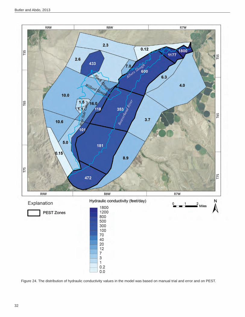
32
Butler and Abdo, 2013
Figure 24. The distribution of hydraulic conductivity values in the model was based on manual trial and error and on PEST.

33
Montana Bureau of Mines and Geology Open-File Report 638
namely Black, Willard, and Albers Sloughs. For each slough, low measurements from an upstream and downstream location measured during the non-irrigation season were used to determine a gain in low per mile. This base low amount was projected
over the stream distance featured in the model and used as a calibration target for each slough. A difference of 15% or less between this value and the model results was considered reasonable. In the steady-state model, the differences between the ield and model results ranged from 9% to 14%,
which met this calibration criterion (table 5).
Transient CalibrationThe transient version of the model used the
aquifer properties from the steady-state model and added the element of time. The transient model was used to simulate time-dependent stresses, such as seasonal irrigation activities. Irrigation ield recharge, canal leakage, and well withdrawals
were modi ied from the steady-state version of the model. Canal and irrigation recharge were applied from April 15 to October 15 to approximate the ir-rigation season; well withdrawal rates were deter-mined based on available pumping data (appendix
Figure 25. Potentiometric surface of layer 1, generated in the steady-state model. The green bars represent cali-bration targets that were within ±15 ft; yellow bars represent targets that were were between 16 and 25.5 ft.
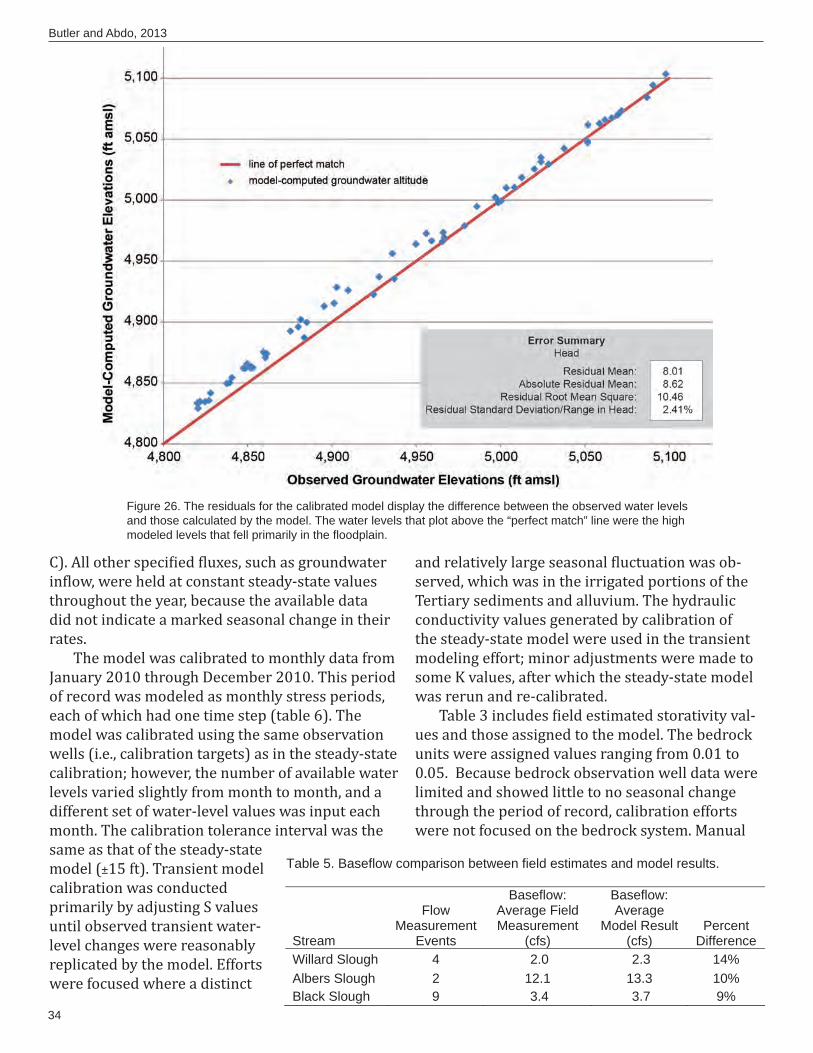
34
Butler and Abdo, 2013
C). All other speci ied luxes, such as groundwater in low, were held at constant steady-state values throughout the year, because the available data did not indicate a marked seasonal change in their rates.
The model was calibrated to monthly data from January 2010 through December 2010. This period of record was modeled as monthly stress periods, each of which had one time step (table 6). The model was calibrated using the same observation wells (i.e., calibration targets) as in the steady-state calibration; however, the number of available water levels varied slightly from month to month, and a different set of water-level values was input each month. The calibration tolerance interval was the same as that of the steady-state model (±15 ft). Transient model calibration was conducted primarily by adjusting S values until observed transient water-level changes were reasonably replicated by the model. Efforts were focused where a distinct
and relatively large seasonal luctuation was ob-served, which was in the irrigated portions of the Tertiary sediments and alluvium. The hydraulic conductivity values generated by calibration of the steady-state model were used in the transient modeling effort; minor adjustments were made to some K values, after which the steady-state model was rerun and re-calibrated.
Table 3 includes ield estimated storativity val-ues and those assigned to the model. The bedrock units were assigned values ranging from 0.01 to 0.05. Because bedrock observation well data were limited and showed little to no seasonal change through the period of record, calibration efforts were not focused on the bedrock system. Manual
Figure 26. The residuals for the calibrated model display the difference between the observed water levels and those calculated by the model. The water levels that plot above the “perfect match” line were the high modeled levels that fell primarily in the fl oodplain.
Table 5. Baseflow comparison between field estimates and model results.
Stream
FlowMeasurement
Events
Baseflow: Average Field Measurement
(cfs)
Baseflow: Average
Model Result (cfs)
PercentDifference
Willard Slough 4 2.0 2.3 14% Albers Slough 2 12.1 13.3 10% Black Slough 9 3.4 3.7 9%
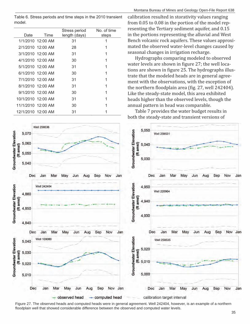
35
Montana Bureau of Mines and Geology Open-File Report 638
calibration resulted in storativity values ranging from 0.05 to 0.08 in the portion of the model rep-resenting the Tertiary sediment aquifer, and 0.15 in the portions representing the alluvial and West Bench volcanic rock aquifers. These values approxi-mated the observed water-level changes caused by seasonal changes in irrigation recharge.
Hydrographs comparing modeled to observed water levels are shown in igure 27; the well loca-tions are shown in igure 25. The hydrographs illus-trate that the modeled heads are in general agree-ment with the observations, with the exception of the northern loodplain area ( ig. 27, well 242404). Like the steady-state model, this area exhibited heads higher than the observed levels, though the annual pattern in head was comparable.
Table 7 provides the water budget results in both the steady-state and transient versions of
Figure 27. The observed heads and computed heads were in general agreement. Well 242404, however, is an example of a northern fl oodplain well that showed considerable difference between the observed and computed water levels.
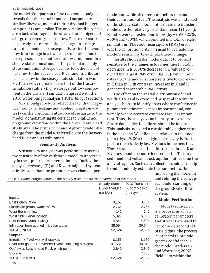
36
Butler and Abdo, 2013
the model. Comparison of the two model budgets reveals that their total inputs and outputs are similar; likewise, most of their individual budget components are similar. The only major differences are a lack of storage in the steady-state budget and a large discrepancy in base low. Due to the nature of a steady-state simulation, changes in storage cannot be modeled; consequently, water that would low into storage in a transient simulation must
be represented as another out low component in a steady-state simulation. In this particular steady-state simulation, storage out low took the form of base low to the Beaverhead River and its tributar-ies; base low in the steady-state simulation was 7,731 acre-ft/yr greater than that of the transient simulation (table 7). The storage out low compo-nent in the transient simulation agreed with the 2010 water budget analysis (Water Budget section).
Model budget results re lect the fact that irriga-tion (i.e., canal leakage and applied irrigation wa-ter) was the predominant source of recharge to the model, demonstrating its considerable in luence on groundwater low within the Lower Beaverhead study area. The primary means of groundwater dis-charge from the model was base low to the Beaver-head River and its tributaries.
Sensitivity AnalysisA sensitivity analysis was performed to assess
the sensitivity of the calibrated model to uncertain-ty in the aquifer parameter estimates. During the analysis, recharge (R) and K were adjusted system-atically, such that one parameter was changed per
model run while all other parameters remained at their calibrated values. The analysis was conducted on the steady-state model rather than the transient model due the relatively brief data record (1 year). R and K were adjusted four times (by +25%, -25%, +50% and -50%), which resulted in a total of eight simulations. The root mean square (RMS) error was the calibration criterion used to evaluate the model’s sensitivity to each parameter change.
Results showed the model output to be most sensitive to the changes in K values, most notably decreases in K. A 50% decrease in K values pro-duced the largest RMS error ( ig. 28), which indi-cates that the model is more sensitive to decreases in K than in R. In contrast, increases in K and R generated comparable RMS errors.
The effect on the spatial distribution of head residuals was also examined. A spatial sensitivity analysis helps to identify areas where con idence in parameter estimates is most important and, con-versely, where accurate estimates are less impor-tant. Thus, the analysis can identify areas where future data collection efforts should be focused. This analysis indicated a considerably higher error in the East and West Benches relative to the lood-plain ( igs. 29, 30); this higher sensitivity is due in part to the relatively low K values in the benches. These results suggest that efforts to estimate K and R values should be more focused on the Tertiary sediment and volcanic rock aquifers rather than the alluvial aquifer. Such data collection could also help to independently estimate the parameters, thus
improving the model it and re ining the concep-tual understanding of the groundwater low system.
Model Veri icationModel veri ication
is a process in which calibrated parameters and stresses are used to reproduce a second set of ield data; the process is intended to provide greater con idence in the model (Anderson and Woessner, 2002). Field data within the
Table 7. Water-budget values in the steady-state and transient versions of the model. Steady-StateBudget Values (ac-ft/yr)
2010 Transient Budget Values (ac-ft/yr)
Inputs East Bench inflow 3,161 3,161 Floodplain groundwater inflow 2,765 2,765 West Bench inflow 142 142 West Side Canal leakage 5,921 5,925 East Bench Canal leakage 4,641 4,594 Infiltration from applied irrigation water 35,994 36,044 TOTAL INPUT 52,624 52,631 Outputs Irrigation + PWS well withdrawals 8,153 8,160 River (net gain at Beaverhead Rock, including sloughs) 41,631 33,918 Outflow at Beaverhead Rock pinch point 2,840 2,840 Storage -- 7,705 TOTAL OUTPUT 52,624 52,622
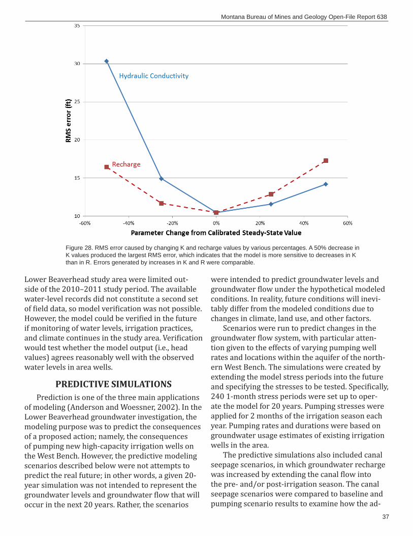
37
Montana Bureau of Mines and Geology Open-File Report 638
Lower Beaverhead study area were limited out-side of the 2010–2011 study period. The available water-level records did not constitute a second set of ield data, so model veri ication was not possible. However, the model could be veri ied in the future if monitoring of water levels, irrigation practices, and climate continues in the study area. Veri ication would test whether the model output (i.e., head values) agrees reasonably well with the observed water levels in area wells.
PREDICTIVE SIMULATIONSPrediction is one of the three main applications
of modeling (Anderson and Woessner, 2002). In the Lower Beaverhead groundwater investigation, the modeling purpose was to predict the consequences of a proposed action; namely, the consequences of pumping new high-capacity irrigation wells on the West Bench. However, the predictive modeling scenarios described below were not attempts to predict the real future; in other words, a given 20-year simulation was not intended to represent the groundwater levels and groundwater low that will occur in the next 20 years. Rather, the scenarios
were intended to predict groundwater levels and groundwater low under the hypothetical modeled conditions. In reality, future conditions will inevi-tably differ from the modeled conditions due to changes in climate, land use, and other factors.
Scenarios were run to predict changes in the groundwater low system, with particular atten-tion given to the effects of varying pumping well rates and locations within the aquifer of the north-ern West Bench. The simulations were created by extending the model stress periods into the future and specifying the stresses to be tested. Speci ically, 240 1-month stress periods were set up to oper-ate the model for 20 years. Pumping stresses were applied for 2 months of the irrigation season each year. Pumping rates and durations were based on groundwater usage estimates of existing irrigation wells in the area.
The predictive simulations also included canal seepage scenarios, in which groundwater recharge was increased by extending the canal low into the pre- and/or post-irrigation season. The canal seepage scenarios were compared to baseline and pumping scenario results to examine how the ad-
Figure 28. RMS error caused by changing K and recharge values by various percentages. A 50% decrease in K values produced the largest RMS error, which indicates that the model is more sensitive to decreases in K than in R. Errors generated by increases in K and R were comparable.
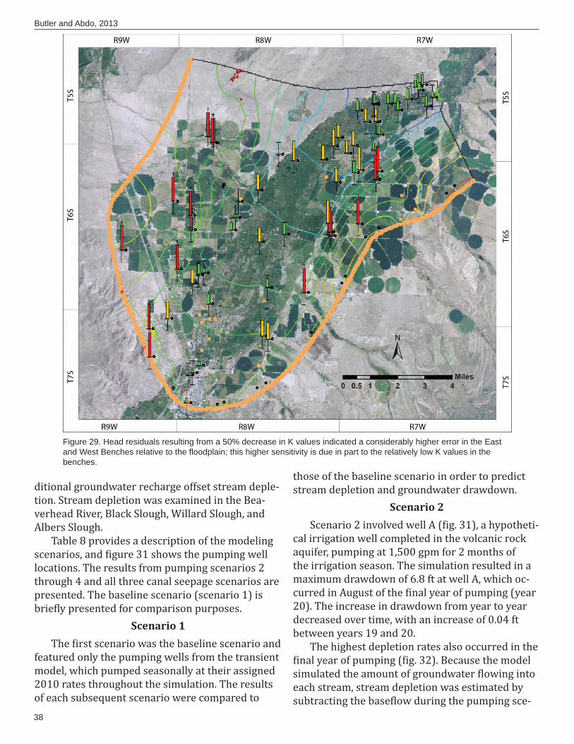
38
Butler and Abdo, 2013
ditional groundwater recharge offset stream deple-tion. Stream depletion was examined in the Bea-verhead River, Black Slough, Willard Slough, and Albers Slough.
Table 8 provides a description of the modeling scenarios, and igure 31 shows the pumping well locations. The results from pumping scenarios 2 through 4 and all three canal seepage scenarios are presented. The baseline scenario (scenario 1) is brie ly presented for comparison purposes.
Scenario 1The irst scenario was the baseline scenario and
featured only the pumping wells from the transient model, which pumped seasonally at their assigned 2010 rates throughout the simulation. The results of each subsequent scenario were compared to
those of the baseline scenario in order to predict stream depletion and groundwater drawdown.
Scenario 2Scenario 2 involved well A ( ig. 31), a hypotheti-
cal irrigation well completed in the volcanic rock aquifer, pumping at 1,500 gpm for 2 months of the irrigation season. The simulation resulted in a maximum drawdown of 6.8 ft at well A, which oc-curred in August of the inal year of pumping (year 20). The increase in drawdown from year to year decreased over time, with an increase of 0.04 ft between years 19 and 20.
The highest depletion rates also occurred in the inal year of pumping ( ig. 32). Because the model
simulated the amount of groundwater lowing into each stream, stream depletion was estimated by subtracting the base low during the pumping sce-
Figure 29. Head residuals resulting from a 50% decrease in K values indicated a considerably higher error in the East and West Benches relative to the fl oodplain; this higher sensitivity is due in part to the relatively low K values in the benches.
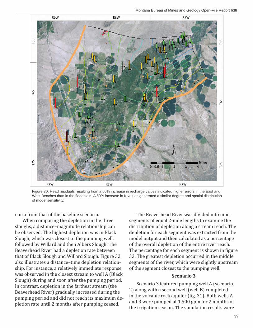
39
Montana Bureau of Mines and Geology Open-File Report 638
nario from that of the baseline scenario.When comparing the depletion in the three
sloughs, a distance–magnitude relationship can be observed. The highest depletion was in Black Slough, which was closest to the pumping well, followed by Willard and then Albers Slough. The Beaverhead River had a depletion rate between that of Black Slough and Willard Slough. Figure 32 also illustrates a distance–time depletion relation-ship. For instance, a relatively immediate response was observed in the closest stream to well A (Black Slough) during and soon after the pumping period. In contrast, depletion in the farthest stream (the Beaverhead River) gradually increased during the pumping period and did not reach its maximum de-pletion rate until 2 months after pumping ceased.
The Beaverhead River was divided into nine segments of equal 2-mile lengths to examine the distribution of depletion along a stream reach. The depletion for each segment was extracted from the model output and then calculated as a percentage of the overall depletion of the entire river reach. The percentage for each segment is shown in igure 33. The greatest depletion occurred in the middle segments of the river, which were slightly upstream of the segment closest to the pumping well.
Scenario 3Scenario 3 featured pumping well A (scenario
2) along with a second well (well B) completed in the volcanic rock aquifer ( ig. 31). Both wells A and B were pumped at 1,500 gpm for 2 months of the irrigation season. The simulation results were
Figure 30. Head residuals resulting from a 50% increase in recharge values indicated higher errors in the East and West Benches than in the fl oodplain. A 50% increase in K values generated a similar degree and spatial distribution of model sensitivity.
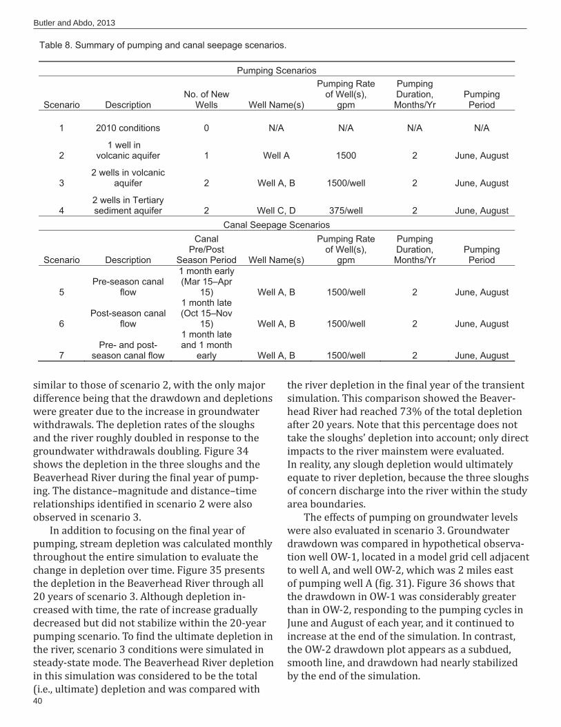
40
Butler and Abdo, 2013
similar to those of scenario 2, with the only major difference being that the drawdown and depletions were greater due to the increase in groundwater withdrawals. The depletion rates of the sloughs and the river roughly doubled in response to the groundwater withdrawals doubling. Figure 34 shows the depletion in the three sloughs and the Beaverhead River during the inal year of pump-ing. The distance–magnitude and distance–time relationships identi ied in scenario 2 were also observed in scenario 3.
In addition to focusing on the inal year of pumping, stream depletion was calculated monthly throughout the entire simulation to evaluate the change in depletion over time. Figure 35 presents the depletion in the Beaverhead River through all 20 years of scenario 3. Although depletion in-creased with time, the rate of increase gradually decreased but did not stabilize within the 20-year pumping scenario. To ind the ultimate depletion in the river, scenario 3 conditions were simulated in steady-state mode. The Beaverhead River depletion in this simulation was considered to be the total (i.e., ultimate) depletion and was compared with
the river depletion in the inal year of the transient simulation. This comparison showed the Beaver-head River had reached 73% of the total depletion after 20 years. Note that this percentage does not take the sloughs’ depletion into account; only direct impacts to the river mainstem were evaluated. In reality, any slough depletion would ultimately equate to river depletion, because the three sloughs of concern discharge into the river within the study area boundaries.
The effects of pumping on groundwater levels were also evaluated in scenario 3. Groundwater drawdown was compared in hypothetical observa-tion well OW-1, located in a model grid cell adjacent to well A, and well OW-2, which was 2 miles east of pumping well A ( ig. 31). Figure 36 shows that the drawdown in OW-1 was considerably greater than in OW-2, responding to the pumping cycles in June and August of each year, and it continued to increase at the end of the simulation. In contrast, the OW-2 drawdown plot appears as a subdued, smooth line, and drawdown had nearly stabilized by the end of the simulation.
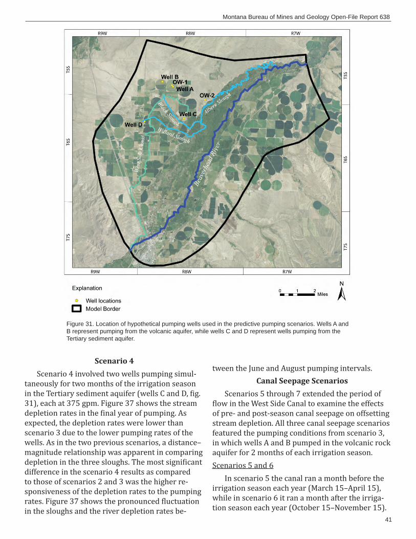
41
Montana Bureau of Mines and Geology Open-File Report 638
Scenario 4Scenario 4 involved two wells pumping simul-
taneously for two months of the irrigation season in the Tertiary sediment aquifer (wells C and D, ig. 31), each at 375 gpm. Figure 37 shows the stream depletion rates in the inal year of pumping. As expected, the depletion rates were lower than scenario 3 due to the lower pumping rates of the wells. As in the two previous scenarios, a distance–magnitude relationship was apparent in comparing depletion in the three sloughs. The most signi icant difference in the scenario 4 results as compared to those of scenarios 2 and 3 was the higher re-sponsiveness of the depletion rates to the pumping rates. Figure 37 shows the pronounced luctuation in the sloughs and the river depletion rates be-
tween the June and August pumping intervals. Canal Seepage Scenarios
Scenarios 5 through 7 extended the period of low in the West Side Canal to examine the effects
of pre- and post-season canal seepage on offsetting stream depletion. All three canal seepage scenarios featured the pumping conditions from scenario 3, in which wells A and B pumped in the volcanic rock aquifer for 2 months of each irrigation season.Scenarios 5 and 6
In scenario 5 the canal ran a month before the irrigation season each year (March 15–April 15), while in scenario 6 it ran a month after the irriga-tion season each year (October 15–November 15).
Figure 31. Location of hypothetical pumping wells used in the predictive pumping scenarios. Wells A and B represent pumping from the volcanic aquifer, while wells C and D represent wells pumping from the Tertiary sediment aquifer.
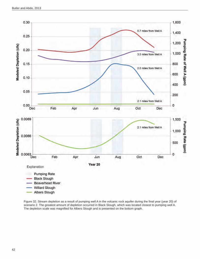
42
Butler and Abdo, 2013
Figure 32. Stream depletion as a result of pumping well A in the volcanic rock aquifer during the fi nal year (year 20) of scenario 2. The greatest amount of depletion occurred in Black Slough, which was located closest to pumping well A. The depletion scale was magnifi ed for Albers Slough and is presented on the bottom graph.
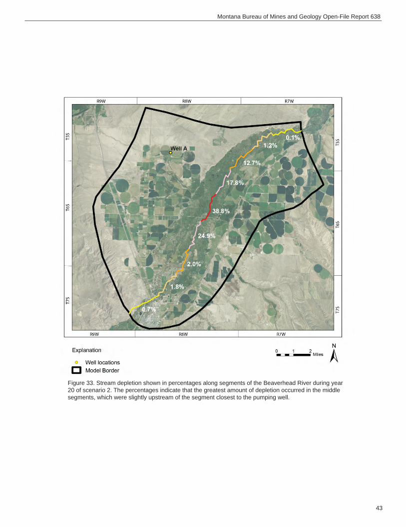
43
Montana Bureau of Mines and Geology Open-File Report 638
Figure 33. Stream depletion shown in percentages along segments of the Beaverhead River during year 20 of scenario 2. The percentages indicate that the greatest amount of depletion occurred in the middle segments, which were slightly upstream of the segment closest to the pumping well.
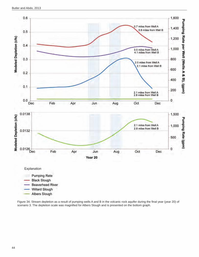
44
Butler and Abdo, 2013
Figure 34. Stream depletion as a result of pumping wells A and B in the volcanic rock aquifer during the fi nal year (year 20) of scenario 3. The depletion scale was magnifi ed for Albers Slough and is presented on the bottom graph.
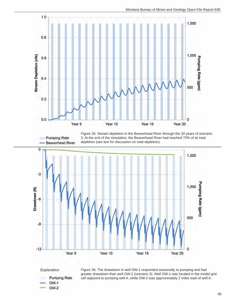
45
Montana Bureau of Mines and Geology Open-File Report 638
Figure 35. Stream depletion in the Beaverhead River through the 20 years of scenario 3. At the end of the simulation, the Beaverhead River had reached 73% of its total depletion (see text for discussion on total depletion).
Figure 36. The drawdown in well OW-1 responded seasonally to pumping and had greater drawdown than well OW-2 (scenario 3). Well OW-1 was located in the model grid cell adjacent to pumping well A, while OW-2 was approximately 2 miles east of well A.
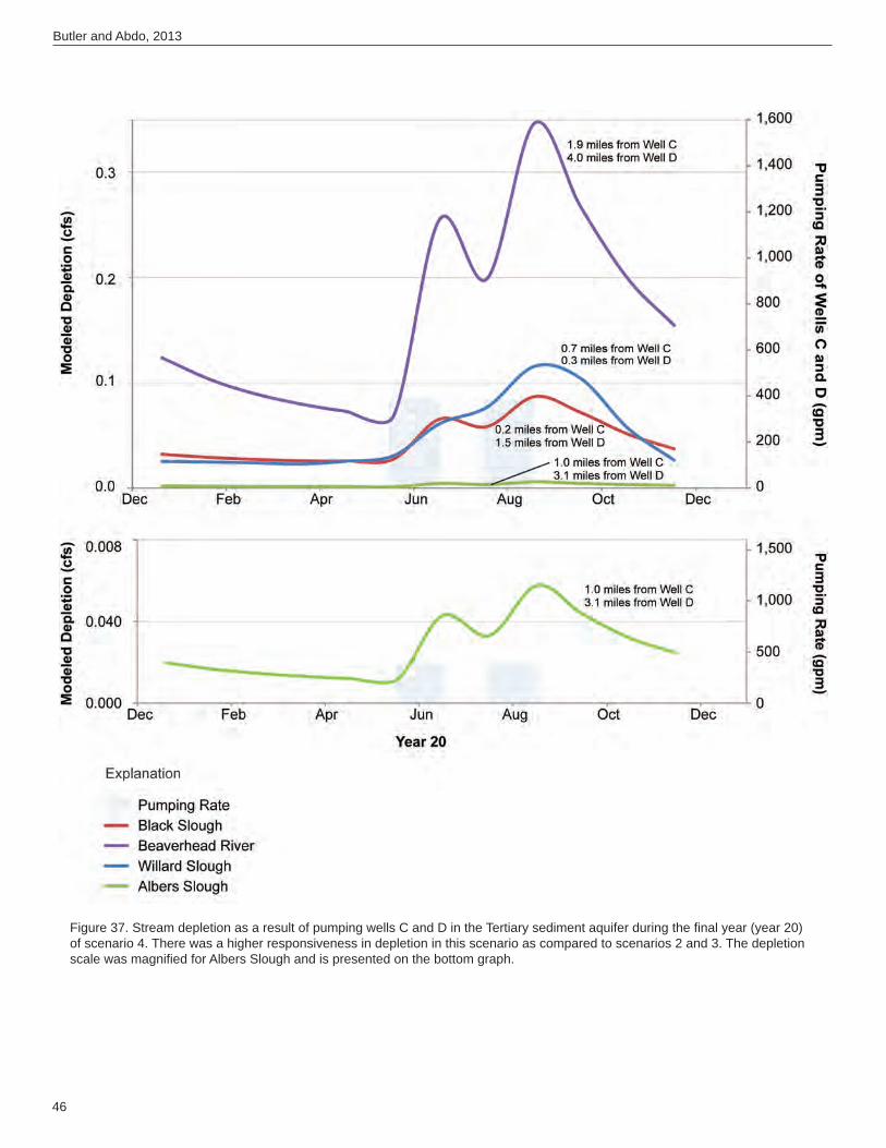
46
Butler and Abdo, 2013
Figure 37. Stream depletion as a result of pumping wells C and D in the Tertiary sediment aquifer during the fi nal year (year 20) of scenario 4. There was a higher responsiveness in depletion in this scenario as compared to scenarios 2 and 3. The depletion scale was magnifi ed for Albers Slough and is presented on the bottom graph.
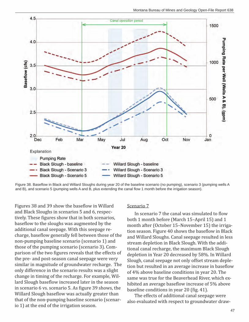
47
Montana Bureau of Mines and Geology Open-File Report 638
Figure 38. Basefl ow in Black and Willard Sloughs during year 20 of the baseline scenario (no pumping), scenario 3 (pumping wells A and B), and scenario 5 (pumping wells A and B, plus extending the canal fl ow 1 month before the irrigation season).
Figures 38 and 39 show the base low in Willard and Black Sloughs in scenarios 5 and 6, respec-tively. These igures show that in both scenarios, base low to the sloughs was augmented by the additional canal seepage. With this seepage re-charge, base low generally fell between those of the non-pumping baseline scenario (scenario 1) and those of the pumping scenario (scenario 3). Com-parison of the two igures reveals that the effects of the pre- and post-season canal seepage were very similar in magnitude of groundwater recharge. The only difference in the scenario results was a slight change in timing of the recharge. For example, Wil-lard Slough base low increased later in the season in scenario 6 vs. scenario 5. As igure 39 shows, the Willard Slough base low was actually greater than that of the non-pumping baseline scenario (scenar-io 1) at the end of the irrigation season.
Scenario 7In scenario 7 the canal was simulated to low
both 1 month before (March 15–April 15) and 1 month after (October 15–November 15) the irriga-tion season. Figure 40 shows the base low in Black and Willard Sloughs. Canal seepage resulted in less stream depletion in Black Slough. With the addi-tional canal recharge, the maximum Black Slough depletion in Year 20 decreased by 58%. In Willard Slough, canal seepage not only offset stream deple-tion but resulted in an average increase in base low of 4% above baseline conditions in year 20. The same was true for the Beaverhead River, which ex-hibited an average base low increase of 5% above baseline conditions in year 20 ( ig. 41).
The effects of additional canal seepage were also evaluated with respect to groundwater draw-
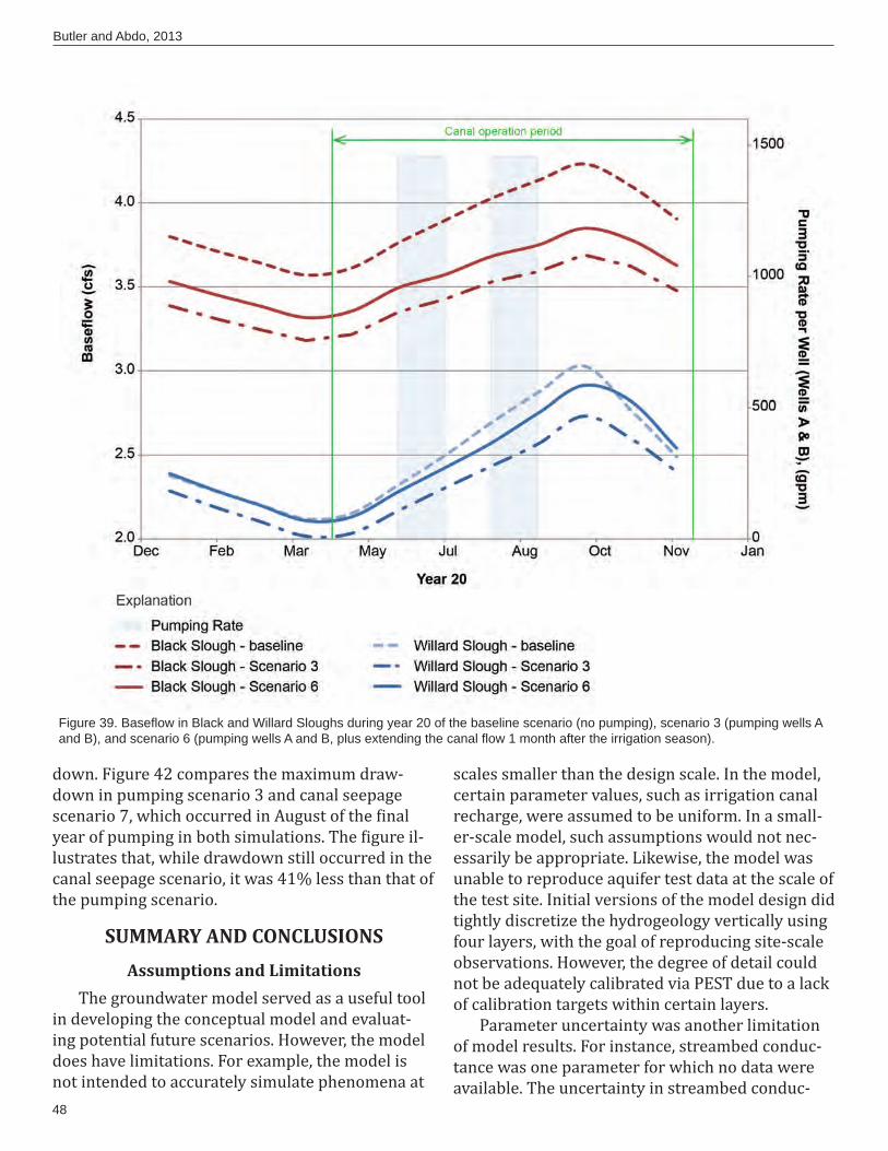
48
Butler and Abdo, 2013
down. Figure 42 compares the maximum draw-down in pumping scenario 3 and canal seepage scenario 7, which occurred in August of the inal year of pumping in both simulations. The igure il-lustrates that, while drawdown still occurred in the canal seepage scenario, it was 41% less than that of the pumping scenario.
SUMMARY AND CONCLUSIONSAssumptions and Limitations
The groundwater model served as a useful tool in developing the conceptual model and evaluat-ing potential future scenarios. However, the model does have limitations. For example, the model is not intended to accurately simulate phenomena at
scales smaller than the design scale. In the model, certain parameter values, such as irrigation canal recharge, were assumed to be uniform. In a small-er-scale model, such assumptions would not nec-essarily be appropriate. Likewise, the model was unable to reproduce aquifer test data at the scale of the test site. Initial versions of the model design did tightly discretize the hydrogeology vertically using four layers, with the goal of reproducing site-scale observations. However, the degree of detail could not be adequately calibrated via PEST due to a lack of calibration targets within certain layers.
Parameter uncertainty was another limitation of model results. For instance, streambed conduc-tance was one parameter for which no data were available. The uncertainty in streambed conduc-
Figure 39. Basefl ow in Black and Willard Sloughs during year 20 of the baseline scenario (no pumping), scenario 3 (pumping wells A and B), and scenario 6 (pumping wells A and B, plus extending the canal fl ow 1 month after the irrigation season).
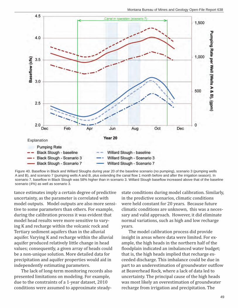
49
Montana Bureau of Mines and Geology Open-File Report 638
tance estimates imply a certain degree of predictive uncertainty, as the parameter is correlated with model outputs. Model outputs are also more sensi-tive to some parameters than others. For example, during the calibration process it was evident that model head results were more sensitive to vary-ing K and recharge within the volcanic rock and Tertiary sediment aquifers than in the alluvial aquifer. Varying K and recharge within the alluvial aquifer produced relatively little change in head values; consequently, a given array of heads could be a non-unique solution. More detailed data for precipitation and aquifer properties would aid in independently estimating parameters.
The lack of long-term monitoring records also presented limitations on modeling. For example, due to the constraints of a 1-year dataset, 2010 conditions were assumed to approximate steady-
state conditions during model calibration. Similarly, in the predictive scenarios, climatic conditions were held constant for 20 years. Because future climatic conditions are unknown, this was a neces-sary and valid approach. However, it did eliminate normal variations, such as high and low recharge years.
The model calibration process did provide insight in areas where data were limited. For ex-ample, the high heads in the northern half of the loodplain indicated an imbalanced water budget;
that is, the high heads implied that recharge ex-ceeded discharge. This imbalance could be due in part to an underestimation of groundwater out low at Beaverhead Rock, where a lack of data led to uncertainty. The principal cause of the high heads was most likely an overestimation of groundwater recharge from irrigation and precipitation. The
Figure 40. Basefl ow in Black and Willard Sloughs during year 20 of the baseline scenario (no pumping), scenario 3 (pumping wells A and B), and scenario 7 (pumping wells A and B, plus extending the canal fl ow 1 month before and after the irrigation season). In scenario 7, basefl ow in Black Slough was 58% higher than in scenario 3. Willard Slough basefl ow increased above that of the baseline scenario (4%) as well as scenario 3.
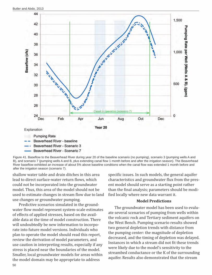
50
Butler and Abdo, 2013
shallow water table and drain ditches in this area lead to direct surface-water return lows, which could not be incorporated into the groundwater model. Thus, this area of the model should not be used to estimate changes in stream low due to land use changes or groundwater pumping.
Predictive scenarios simulated in the ground-water low model represent system-scale estimates of effects of applied stresses, based on the avail-able data at the time of model construction. There will undoubtedly be new information to incorpo-rate into future model versions. Individuals who plan to operate the model should read this report, review the derivation of model parameters, and use caution in interpreting results, especially if any stress is placed near the boundaries of the model. Smaller, local groundwater models for areas within the model domain may be appropriate to address
speci ic issues. In such models, the general aquifer characteristics and groundwater lux from the pres-ent model should serve as a starting point rather than the inal analysis; parameters should be modi-ied locally where new data warrant it.
Model PredictionsThe groundwater model has been used to evalu-
ate several scenarios of pumping from wells within the volcanic rock and Tertiary sediment aquifers on the West Bench. Pumping scenario results showed two general depletion trends with distance from the pumping center: the magnitude of depletion decreased, and the timing of depletion was delayed. Instances in which a stream did not it these trends were likely due to the model’s sensitivity to the streambed conductance or the K of the surrounding aquifer. Results also demonstrated that the stream
Figure 41. Basefl ow to the Beaverhead River during year 20 of the baseline scenario (no pumping), scenario 3 (pumping wells A and B), and scenario 7 (pumping wells A and B, plus extending canal fl ow 1 month before and after the irrigation season). The Beaverhead River basefl ow exhibited an increase of about 5% above baseline conditions when the canal fl ow was extended 1 month before and after the irrigation season (scenario 7).
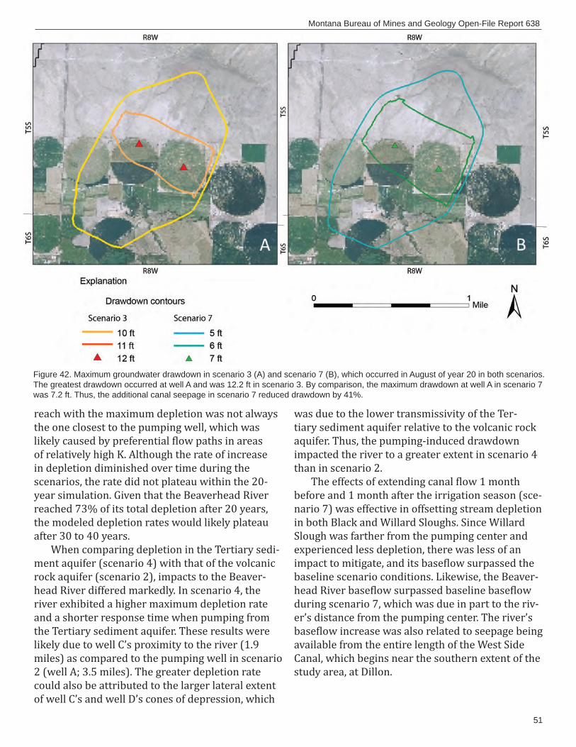
51
Montana Bureau of Mines and Geology Open-File Report 638
reach with the maximum depletion was not always the one closest to the pumping well, which was likely caused by preferential low paths in areas of relatively high K. Although the rate of increase in depletion diminished over time during the scenarios, the rate did not plateau within the 20-year simulation. Given that the Beaverhead River reached 73% of its total depletion after 20 years, the modeled depletion rates would likely plateau after 30 to 40 years.
When comparing depletion in the Tertiary sedi-ment aquifer (scenario 4) with that of the volcanic rock aquifer (scenario 2), impacts to the Beaver-head River differed markedly. In scenario 4, the river exhibited a higher maximum depletion rate and a shorter response time when pumping from the Tertiary sediment aquifer. These results were likely due to well C’s proximity to the river (1.9 miles) as compared to the pumping well in scenario 2 (well A; 3.5 miles). The greater depletion rate could also be attributed to the larger lateral extent of well C’s and well D’s cones of depression, which
was due to the lower transmissivity of the Ter-tiary sediment aquifer relative to the volcanic rock aquifer. Thus, the pumping-induced drawdown impacted the river to a greater extent in scenario 4 than in scenario 2.
The effects of extending canal low 1 month before and 1 month after the irrigation season (sce-nario 7) was effective in offsetting stream depletion in both Black and Willard Sloughs. Since Willard Slough was farther from the pumping center and experienced less depletion, there was less of an impact to mitigate, and its base low surpassed the baseline scenario conditions. Likewise, the Beaver-head River base low surpassed baseline base low during scenario 7, which was due in part to the riv-er’s distance from the pumping center. The river’s base low increase was also related to seepage being available from the entire length of the West Side Canal, which begins near the southern extent of the study area, at Dillon.
Figure 42. Maximum groundwater drawdown in scenario 3 (A) and scenario 7 (B), which occurred in August of year 20 in both scenarios. The greatest drawdown occurred at well A and was 12.2 ft in scenario 3. By comparison, the maximum drawdown at well A in scenario 7 was 7.2 ft. Thus, the additional canal seepage in scenario 7 reduced drawdown by 41%.
52
Butler and Abdo, 2013
RecommendationsModel recommendations concur with those
of the Lower Beaverhead study (Abdo and oth-ers, 2013). For instance, study recommendations include exploratory drilling to the north and south of the identi ied volcanic rock body, which would better characterize the aquifer’s extent and devel-opment potential. Such a characterization would reduce model uncertainty and thereby enhance model results.
The Lower Beaverhead study recommendations also include the development of a management plan with regard to groundwater withdrawals from the volcanic rock aquifer. To this end, the numerical model could be a useful tool in the process. It could be used to delineate zones of stream depletion; that is, zones in which a pumping well (pumping at a speci ied rate for a speci ied duration) would de-plete the stream by a certain percentage. As dem-onstrated in the model results, stream depletion can continue after pumping ceases; the depletion rate can be even greater than the rate during pump-ing (Jenkins, 1968; Kendy and Bredehoeft, 2006). Such a delayed response can be dif icult to predict without the aid of a model; thus, the model would be a key component of a management plan which minimizes effects to the stream.
The canal seepage scenario results suggest that early and late-season canal seepage is an effective offset measure to stream depletion. However, in applying the model results to practice, the proxim-ity of the pumping well(s) and the stream(s) to the given canal should be considered. The effectiveness of the approach could also depend on site-speci ic conditions such as streambed and canal bed con-ductance values, as well as the variations of hydrau-lic conductivity and storativity values of the under-lying aquifer(s). Weather conditions are another factor that could impact the practicality of extended canal operations, given that colder temperatures and greater precipitation reduce seepage loss, and frozen soil impedes recharge to the subsurface.
Several years after publication of this report, a post-audit of the model may be bene icial. The post-audit would use long-term monitoring data to test whether the model’s predictions were reason-able (Anderson and Woessner, 2002). It is also rec-ommended that if site-speci ic decisions are need-ed, more detailed data from that site be collected
and incorporated into the decision-making process. In particular, if geologic conditions are encountered that differ from those assumed in the model (e.g., the extent of the volcanic rock aquifer), the model must be modi ied to incorporate such features. Fur-ther data collection would also bene it the existing large-scale model, because such data would make independent parameter estimation more feasible.
REFERENCES
Abdo, G., Butler, J., Myse, T., Wheaton, J., Snyder, D., Metesh, J., and Shaw, G., 2013, Hydrogeologic investigation of the Lower Beaverhead study area, Beaverhead County, Montana, MBMG Open-File Report 637.
Alt, D., and Hyndman, D., 1986, Roadside Geology of Montana: Missoula, MT, Mountain Press Publishing Company, 427 p.
Anderson, M.P., and Woessner, W.W., 2002, Applied groundwater modeling: Simulation of low and ad-vective transport: New York, Academic Press, Inc.
Aquaveo, LLC, 2010. Groundwater Modeling System (GMS), version 7.1.
ASTM, 2004, Standard guide for application of a ground-water low model to a site-speci ic problem, D5447-04: West Conshohocken, PA, ASTM Interna-tional, November 2004.
Briar, D.W., and Madison, J.P., 1992, Hydrogeology of the Helena valley- ill aquifer system, west-central Mon-tana: U.S. Geological Survey Water-Resources In-vestigation Report 92-4023, 1 plate, scale 1:48,800.
Cooper, H.H., Jr., and Jacob, C.E., 1946, A generalized graphical method for evaluating formation con-stants and summarizing well- ield history,:Trans. American Geophysical Union, v. 27, no. 4, p. 526–534.
Doherty, J., 2010, PEST model-independent parameter estimation user manual (5th ed.): Brisbane, Aus-tralia, Watermark Numerical Computing, 336 p., http://www.pesthomepage.org [accessed March 16, 2011].
Fetter, C.W., 2001, Applied hydrogeology (4th ed.): Up-per Saddle River, N.J., Prentice Hall, p. 185.
GPS Visualizer, 2011, online mapping utility, http://www.gpsvisualizer.com/ [accessed January 2011].
Harbaugh, A.W., Banta, E.R., Hill, M.C., and McDonald, M.G., 2000, MODFLOW-2000, the U.S. Geological Survey modular ground-water model—User guide
53
Montana Bureau of Mines and Geology Open-File Report 638
to modularization concepts and the Ground-Water Flow Process: U.S. Geological Survey Open-File Report 00-92, 121 p.
Jenkins, C.T., 1968, Computation of rate and volume of stream depletion by wells, in U.S. Geological Survey techniques of water resources investigations, book 4, p. 17.
Kauffman, M.H., 1999, An investigation of ground-wa-ter–surface water interaction in the Flint Creek Val-ley, Granite County, Montana: M.S. Thesis, Montana State University, Bozeman, MT.
Kendy, E., and Bredehoeft, J.D., 2006, Transient effects of groundwater pumping and surface-water irrigation returns on stream low: Water Resources Research, v. 42, W08415, doi: 0.1029/2005WR004792.
Mandle, R.J., 2002. Groundwater Modeling Guidance, Michigan Department of Environmental Quality, Draft 1.0, 54 p.
Montana Bureau of Mines and Geology, 2008, Final case study report to the 60th Legislature Water Policy Interim Committee (with public comments), avail-able online at http://www.mbmg.mtech.edu/gwip/gwip_pdf/hb831book_appendix.pdf [accessed October 31, 2011].
Montana Department of Natural Resources and Con-servation, 2003, Montana’s basin closures and controlled groundwater areas, December 2003: Montana Department of Natural Resources Water Resources Division, Water Rights Bureau, Helena, Mont., available online at http://www.dnrc.mt.gov/wrd/water_rts/appro_info/basinclose-cgw_areas.pdf [accessed October 2010].
Montana Department of Revenue, Montana State Li-brary, Revenue Final Land Unit (FLU) Classi ication, v. 2010, Helena, Mont., available online at http://nris.mt.gov/nsdi/nris/mdb/revenue_ lu.zip [ac-cessed October 2010].
Montana Supreme Court, 2006, Trout Unlimited v. Mon-tana Department of Natural Resources and Conser-vation, Decision in case number 05-069, 331 Mont. 483, 33 P. 3d 224.
Rumbaugh, James O., 2007. Guide to using groundwater vistas, Version 5, Environmental Simulations, Inc., p.188.
Ruppel, E.T., O’Neill, J.M., and Lopez, D.A., 1993, Geologic map of the Dillon 1°x2° quadrangle, Idaho and Montana: U.S. Geological Survey Miscellaneous Investigations Series Map I-183-H, scale 1:250,000.
SNOTEL (2011), http://www.wcc.nrcs.usda.gov/nwcc/site?sitenum=656&state=mt [accessed November 2010].
U.S. Bureau of Reclamation, 2008, East Bench main canal seepage investigations, 2007, Clark Canyon Project, Dillon, Montana, Great Plains Region, U.S. Department of the Interior, Technical Memoran-dum No. 86-68210-S&T-2008-01, 6 p.
U.S. Geological Survey, 2009, 1/3-Arc second national elevation dataset, Sioux Falls, S. Dak., downloaded April 1, 2010 from http://nationalmap.gov/view-ers.html.
Uthman, W., and Beck, J., 1998, Hydrogeology of the Upper Beaverhead Basin near Dillon, Montana: Montana Department of Natural Resources and Conservation with Montana Bureau of Mines and Geology Open-File Report 384.
van der Kamp, G., 1989: Calculation of constant-rate drawdowns from stepped-rate pumping tests, Ground Water, v. 27, no. 2, p. 175–183.
Vuke, S.M., Porter, K.W., Lonn, J.D., and Lopez, D.A., 2007, Geologic map of Montana: Montana Bureau of Mines and Geology Geologic Map 62, 73 p., 2 sheets, scale 1:500,00.
Waren, K., 1998, Groundwater conditions at the Hayes Creek Temporary Controlled Groundwater Area: unpublished Montana Department of Natural Re-sources and Conservation report, 42 p. [Accessed 12/19/2011 from http://www.dnrc.mt.gov/wrd/water_rts/cgwa/hayes_creek/hayes_creek_CGWA_report.pdf]
Weight, W.D., and Snyder, D., 2007, Beaverhead val-ley groundwater study, inal report, USBR Fund 526091: Butte, Mont., Montana Tech of the Uni-versity of Montana, submitted to the U.S. Bureau of Reclamation.
Western Regional Climate Center, Dillon WMCE, Mon-tana (242409), available online at http://www.wrcc.dri.edu/cgi-bin/cliMAIN.pl?mt2409 [accessed January 2011].


55
Montana Bureau of Mines and Geology Open-File Report 638
APPENDIX AModel File Index

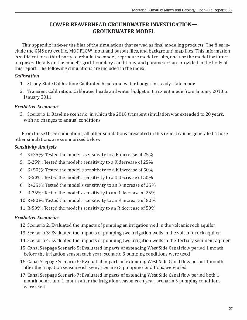
57
Montana Bureau of Mines and Geology Open-File Report 638
LOWER BEAVERHEAD GROUNDWATER INVESTIGATIONGROUNDWATER MODEL
This appendix indexes the iles of the simulations that served as inal modeling products. The iles in-clude the GMS project ile, MODFLOW input and output iles, and background map iles. This information is suf icient for a third party to rebuild the model, reproduce model results, and use the model for future purposes. Details on the model’s grid, boundary conditions, and parameters are provided in the body of this report. The following simulations are included in the index:Calibration
1. Steady-State Calibration: Calibrated heads and water budget in steady-state mode2. Transient Calibration: Calibrated heads and water budget in transient mode from January 2010 to
January 2011
Predictive Scenarios3. Scenario 1: Baseline scenario, in which the 2010 transient simulation was extended to 20 years,
with no changes to annual conditions
From these three simulations, all other simulations presented in this report can be generated. Those other simulations are summarized below. Sensitivity Analysis
4. K+25%: Tested the model’s sensitivity to a K increase of 25%5. K-25%: Tested the model’s sensitivity to a K decrease of 25%6. K+50%: Tested the model’s sensitivity to a K increase of 50%7. K-50%: Tested the model’s sensitivity to a K decrease of 50%8. R+25%: Tested the model’s sensitivity to an R increase of 25%9. R-25%: Tested the model’s sensitivity to an R decrease of 25%10. R+50%: Tested the model’s sensitivity to an R increase of 50%11. R-50%: Tested the model’s sensitivity to an R decrease of 50%
Predictive Scenarios12. Scenario 2: Evaluated the impacts of pumping an irrigation well in the volcanic rock aquifer13. Scenario 3: Evaluated the impacts of pumping two irrigation wells in the volcanic rock aquifer14. Scenario 4: Evaluated the impacts of pumping two irrigation wells in the Tertiary sediment aquifer15. Canal Seepage Scenario 5: Evaluated impacts of extending West Side Canal low period 1 month
before the irrigation season each year; scenario 3 pumping conditions were used16. Canal Seepage Scenario 6: Evaluated impacts of extending West Side Canal low period 1 month
after the irrigation season each year; scenario 3 pumping conditions were used17. Canal Seepage Scenario 7: Evaluated impacts of extending West Side Canal low period both 1
month before and 1 month after the irrigation season each year; scenario 3 pumping conditions were used
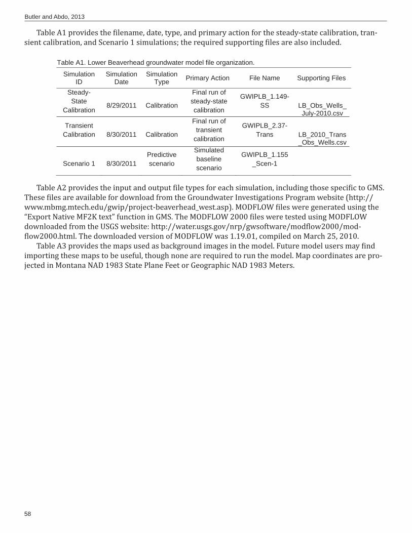
58
Butler and Abdo, 2013
Table A1 provides the ilename, date, type, and primary action for the steady-state calibration, tran-sient calibration, and Scenario 1 simulations; the required supporting iles are also included.
Table A2 provides the input and output ile types for each simulation, including those speci ic to GMS. These iles are available for download from the Groundwater Investigations Program website (http://www.mbmg.mtech.edu/gwip/project-beaverhead_west.asp). MODFLOW iles were generated using the “Export Native MF2K text” function in GMS. The MODFLOW 2000 iles were tested using MODFLOW downloaded from the USGS website: http://water.usgs.gov/nrp/gwsoftware/mod low2000/mod-low2000.html. The downloaded version of MODFLOW was 1.19.01, compiled on March 25, 2010.
Table A3 provides the maps used as background images in the model. Future model users may ind importing these maps to be useful, though none are required to run the model. Map coordinates are pro-jected in Montana NAD 1983 State Plane Feet or Geographic NAD 1983 Meters.
Table A1. Lower Beaverhead groundwater model file organization.
SimulationID
SimulationDate
SimulationType Primary Action File Name Supporting Files
Steady-State
Calibration8/29/2011 Calibration
Final run of steady-statecalibration
GWIPLB_1.149-SS LB_Obs_Wells_
July-2010.csv
Transient Calibration 8/30/2011 Calibration
Final run of transient
calibration
GWIPLB_2.37-Trans LB_2010_Trans
_Obs_Wells.csv
Scenario 1 8/30/2011 Predictive scenario
Simulatedbaselinescenario
GWIPLB_1.155_Scen-1
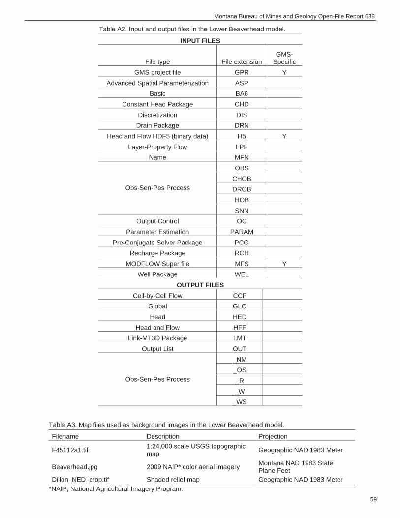
59
Montana Bureau of Mines and Geology Open-File Report 638
Table A2. Input and output files in the Lower Beaverhead model.
INPUT FILES
File type File extension GMS-
SpecificGMS project file GPR Y
Advanced Spatial Parameterization ASP Basic BA6
Constant Head Package CHD Discretization DIS
Drain Package DRN Head and Flow HDF5 (binary data) H5 Y
Layer-Property Flow LPF Name MFN
Obs-Sen-Pes Process
OBS CHOB DROB HOB SNN
Output Control OC Parameter Estimation PARAM
Pre-Conjugate Solver Package PCG Recharge Package RCH
MODFLOW Super file MFS Y Well Package WEL
OUTPUT FILES Cell-by-Cell Flow CCF
Global GLO Head HED
Head and Flow HFF Link-MT3D Package LMT
Output List OUT
Obs-Sen-Pes Process
_NM _OS _R _W
_WS
Table A3. Map files used as background images in the Lower Beaverhead model.
Filename Description Projection
F45112a1.tif 1:24,000 scale USGS topographic map Geographic NAD 1983 Meter
Beaverhead.jpg 2009 NAIP* color aerial imagery Montana NAD 1983 State Plane Feet
Dillon_NED_crop.tif Shaded relief map Geographic NAD 1983 Meter *NAIP, National Agricultural Imagery Program.


61
Montana Bureau of Mines and Geology Open-File Report 638
APPENDIX B Estimating Irrigation Recharge (IR) in the Groundwater Budget

63
Montana Bureau of Mines and Geology Open-File Report 638
LOWER BEAVERHEAD GROUNDWATER INVESTIGATION GROUNDWATER MODEL
This appendix details the approach used to estimate groundwater recharge from applied irrigation water within the Lower Beaverhead study area. Irrigation recharge (IR) was one component of the mod-el’s groundwater budget, which is discussed in the Groundwater Budget section of the report. The result-ing recharge estimates were used as model input values and also as water budget targets during model calibration.
The procedure for estimating irrigation recharge was as follows:1. The percent ef iciency was obtained from the Natural Resources Conservation Service (NRCS) for
each irrigation type (Morris, oral commun., 2011). The ef iciencies were 80%, 65%, and 35% for pivot, wheelline, and lood (respectively).
2. The Irrigation Water Requirements (IWR) Crop Data Summaries supplied by the NRCS were reviewed (Morris, written commun., 2011; appendix D). The IWR values were calculated using the Blaney Criddle (TR21) method.
3. For each crop type and irrigation type, the Net Irrigation Requirement (table B1) was taken from the IWR records and divided by the ef iciency percentage (step 1) to calculate the Gross Irrigation Requirement.
4. The Effective Precipitation was added to the Gross Irrigation Requirement in order to calculate the total amount of water being applied to an irrigated parcel (“Total Applied” in table B1).
5. The Total ET was then subtracted from the total amount of water being applied to calculate the amount of water available for recharge to the groundwater system (“Annual Recharge” in table B1).
6. The total acreage for each individual irrigated parcel was calculated using the Statewide FLU geo-database (Montana Department of Revenue, 2010).
7. For pivot and wheelline areas, it was assumed that 75% of those areas were irrigating alfalfa hay, 20% spring wheat, and 5% potatoes. For lood irrigation, it was assumed that 80% was grass hay and the remaining 20% was alfalfa hay. The majority of these percentages were supplied by the NRCS (Morris, oral commun., 2011).
8. Using the Annual Recharge values (table B1), acreage per parcel, and the crop type percentages, the annual amount of groundwater recharge was calculated for each individual parcel within the study area. These per-parcel recharge values were added together to obtain the total irrigation recharge within the study area. This recharge value served as the irrigation recharge component (IR) of the model’s groundwater budget (see the Groundwater Budget section of report).
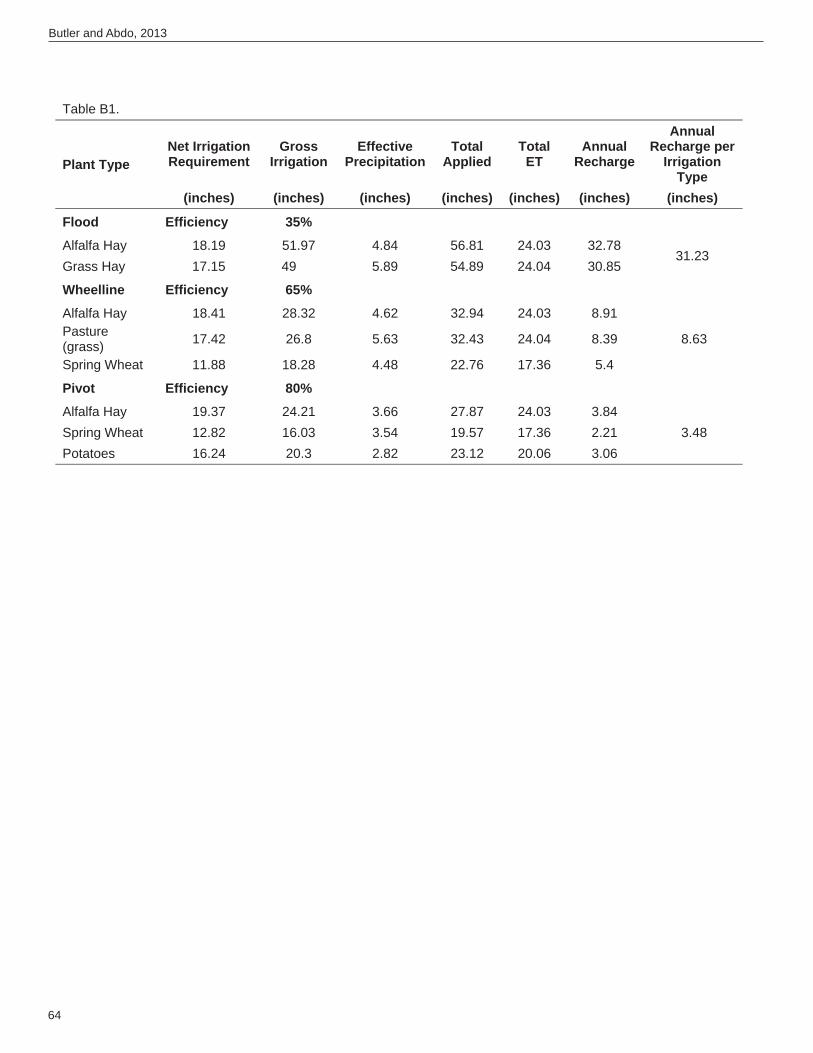
64
Butler and Abdo, 2013
Table B1.
Plant Type Net Irrigation Requirement
GrossIrrigation
Effective Precipitation
TotalApplied
TotalET
Annual Recharge
Annual Recharge per
IrrigationType
(inches) (inches) (inches) (inches) (inches) (inches) (inches)
Flood Efficiency 35%
Alfalfa Hay 18.19 51.97 4.84 56.81 24.03 32.78 31.23
Grass Hay 17.15 49 5.89 54.89 24.04 30.85
Wheelline Efficiency 65%
Alfalfa Hay 18.41 28.32 4.62 32.94 24.03 8.91
8.63 Pasture(grass) 17.42 26.8 5.63 32.43 24.04 8.39
Spring Wheat 11.88 18.28 4.48 22.76 17.36 5.4
Pivot Efficiency 80%
Alfalfa Hay 19.37 24.21 3.66 27.87 24.03 3.84 3.48 Spring Wheat 12.82 16.03 3.54 19.57 17.36 2.21
Potatoes 16.24 20.3 2.82 23.12 20.06 3.06
65
Montana Bureau of Mines and Geology Open-File Report 638
APPENDIX C Estimating Well Withdrawals (WW) in the
Groundwater Budget

67
Montana Bureau of Mines and Geology Open-File Report 638
LOWER BEAVERHEAD GROUNDWATER INVESTIGATION GROUNDWATER MODEL
This appendix details the approach used to estimate groundwater withdrawals from irrigation and public water supply (PWS) wells within the Lower Beaverhead study area. Well withdrawals (WW) constituted one component of the model’s groundwater budget, which is discussed in the Groundwater Budget section of the report. The resulting estimates were used as model input values and also as water budget targets during model calibration.
As a irst step in the approach, all wells classi ied as “irrigation” or “PWS” in the study area were in-ventoried in the GWIC database (http://mbmggwic.mtech.edu). Available water rights records and permit applications for these wells were also inventoried, which included a search of the records within DNRC’s Water Rights Bureau. The remainder of this discussion categorizes the approach by well type.Irrigation Wells
To estimate irrigation well withdrawals, aerial photos were examined to determine whether the water right was being used; for instance, if the aerial photo was taken during the irrigation season and showed fallow land, the well was not considered to be in use. If the well did appear to be in use, the irrigation type ( lood, pivot, or sprinkler) was also identi ied in the photo. The amount of water required annually by the crop was then estimated for each water right holder’s property. This amount was calculated using the total crop acreage listed in the Water Right abstract or permit application, along with the per-acre crop requirement determined from the NRCS Irrigation Water Requirement approach, discussed in appendix B. The annual water requirement was termed the “calculated volume.”
For permitted wells that were supplemental to surface-water sources, the calculated volume was compared with the surface-water allotment use (where water-use records were available). The well with-drawal volume was assumed to make up the difference between the calculated volume and the volume of surface water used. For water rights with no surface-water allotment, the calculated volume was assumed to be fully supplied by the well during the irrigation season, unless transducer data indicated otherwise. At select sites, a pressure transducer was installed in the pumping well or an adjacent monitoring well, and the pumping frequency was estimated based on drawdown in the water-level record.
For unpermitted wells, the acreage of irrigated land was unknown and the volume of water could not be calculated; consequently, the entire water right (as stated in the well permit application) was assumed to be supplied by the irrigation well, unless transducer data indicated otherwise.
Last, for wells without an associated permit application or water rights record, water withdrawals were roughly based on the well yields (i.e., pumping rates) reported in driller’s logs. A water-use volume was calculated based on the assumption that the irrigation well pumped for approximately 2 months of the year at the given pumping rate, because 2 months was deemed a realistic pumping period during the irrigation season.
For some irrigation wells, the estimated pumping rates resulted in greater drawdown than was shown in nearby observation wells. Consequently, such pumping rates were reduced during calibration in order to best match the observed water levels. These reductions were deemed acceptable given the inherent uncertainty in the original pumping-rate estimates (as discussed under Limitations, below). PWS wells
For the City of Dillon’s PWS wells, monthly water-use records were provided by the City of Dillon; therefore, water-use estimation was not required. For subdivision PWS wells, each subdivision was irst veri ied in the Montana Cadastral system and through aerial photo inspection. If the development was veri ied, the PWS well withdrawal was assumed to equal the subdivision’s entire water right. 2010 Transient Model
The transient model was divided into monthly increments, and so well withdrawals were divided into monthly percentages. As stated previously, monthly water-use records were provided by City of Dillon; these values were directly input into the transient model. The City PWS well percentages were applied to

68
Butler and Abdo, 2013
the subdivision PWS wells, under the assumption that water use in the subdivisions was proportional to that of the City.
For irrigation wells, an average percentage was applied to each month of the irrigation season, with the exception of April and October; for those 2 months, the percentage was set to half the monthly aver-age, under the assumption that wells were used only in the second half of April and the irst half of Octo-ber. This approach resulted in a monthly percentage of 8.33% for April and October, and 16.66% for the months of May through September.Limitations
A degree of uncertainty is inherent in these well withdrawal estimates due to simplifying assumptions that were made. For instance, the withdrawals could be an underestimate, because wells likely existed that were unknown to the investigators. This likelihood is based on the fact that neither permits nor wa-ter-right records could be found for irrigation wells that were known to exist (through personal contact with the well owners). On the other hand, some wells were assumed to use their entire water right when they may have used much less; therefore, such well withdrawals could be overestimates.

69
Montana Bureau of Mines and Geology Open-File Report 638
APPENDIX DNatural Resources Conservation Service (NRCS)
Irrigation Water Requirements–Crop Data Summaries
(Morris, written commun., 2011)

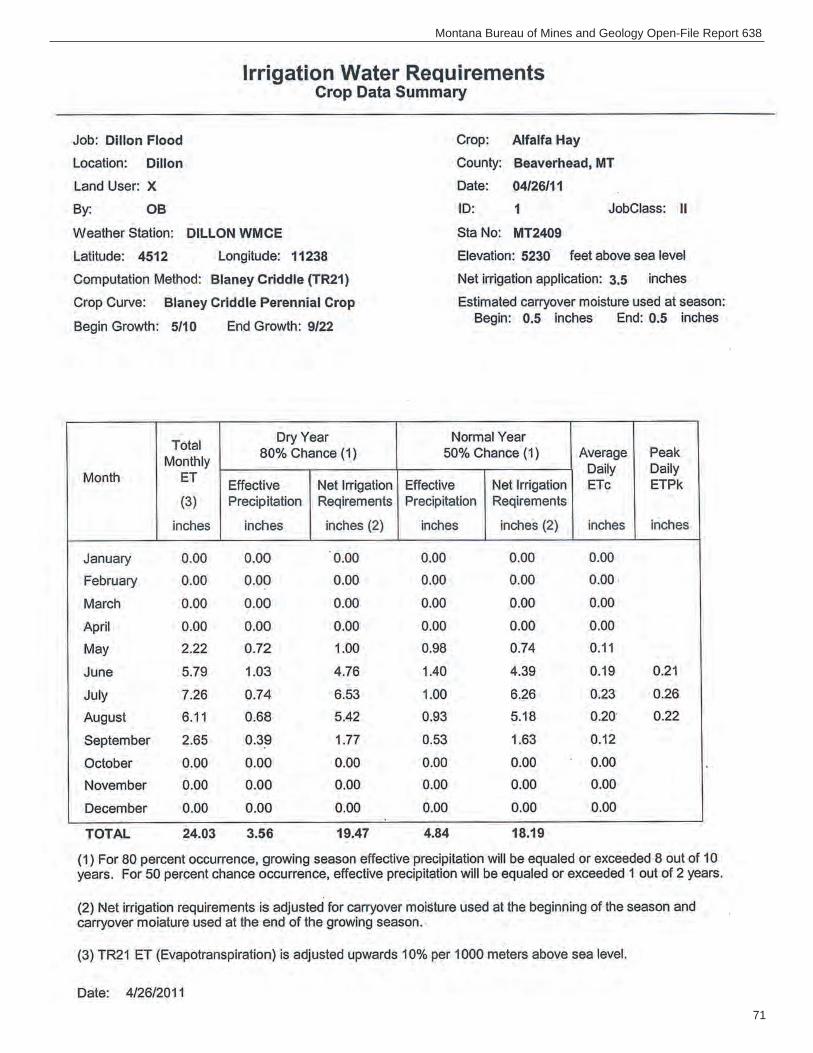
71
Montana Bureau of Mines and Geology Open-File Report 638
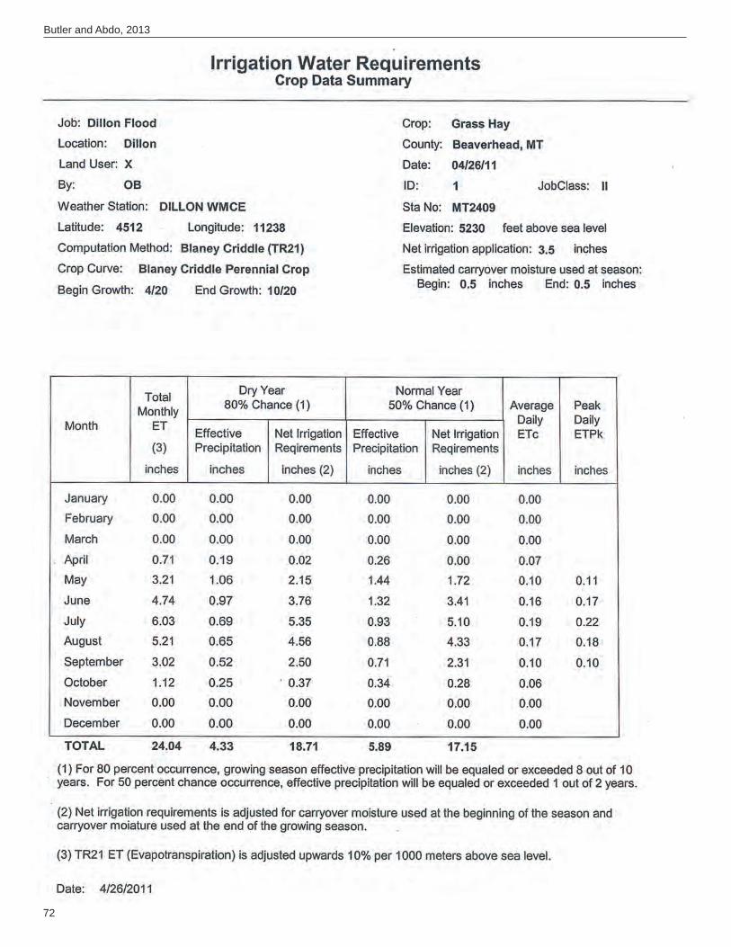
72
Butler and Abdo, 2013
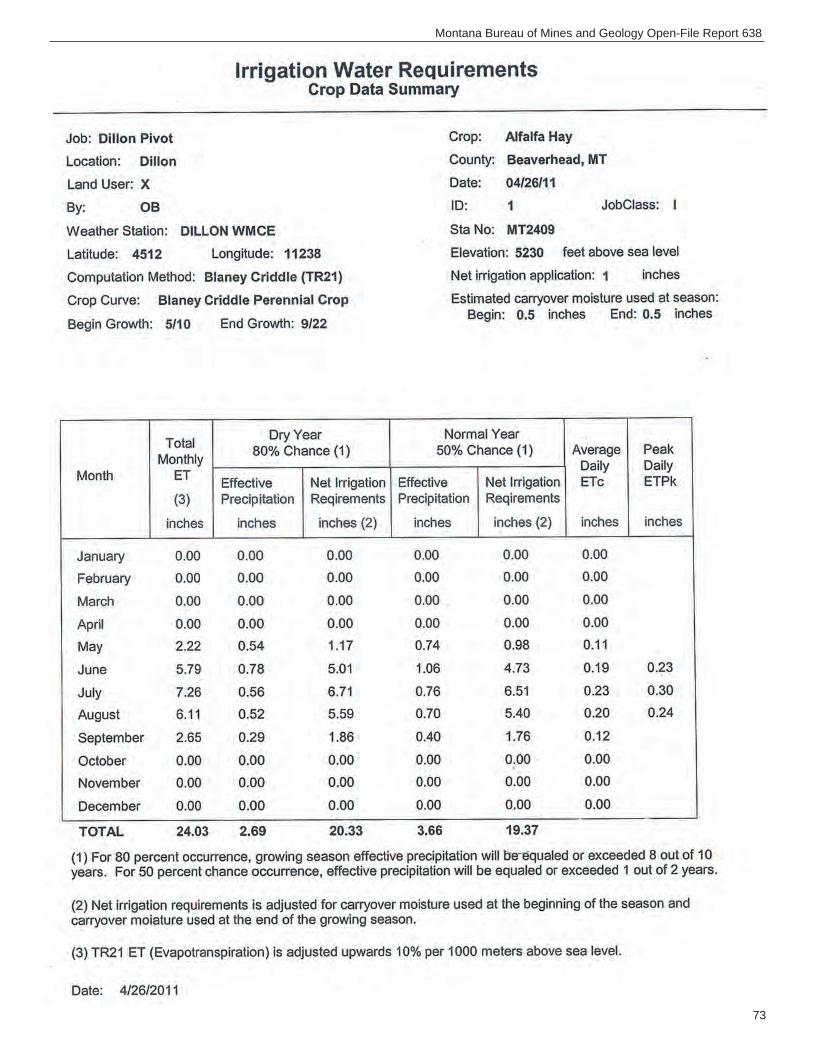
73
Montana Bureau of Mines and Geology Open-File Report 638
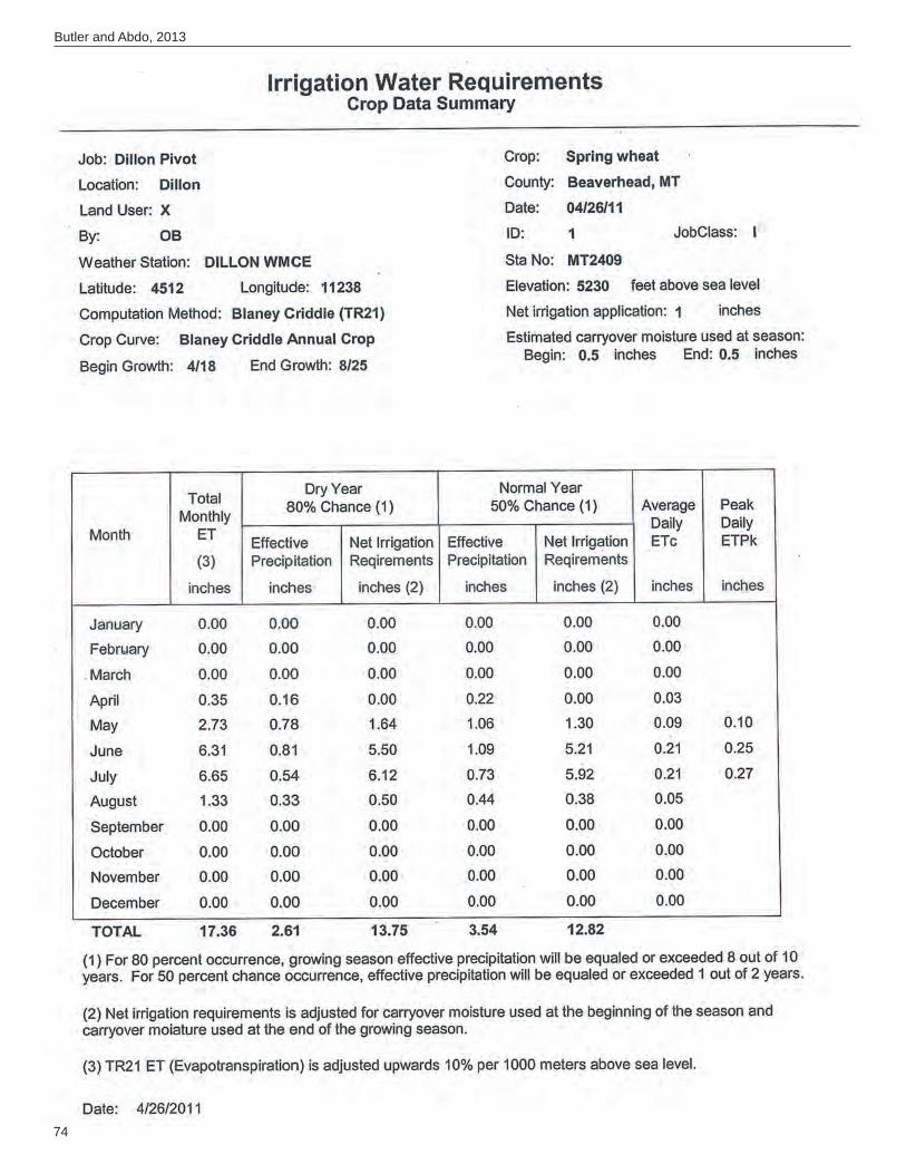
74
Butler and Abdo, 2013
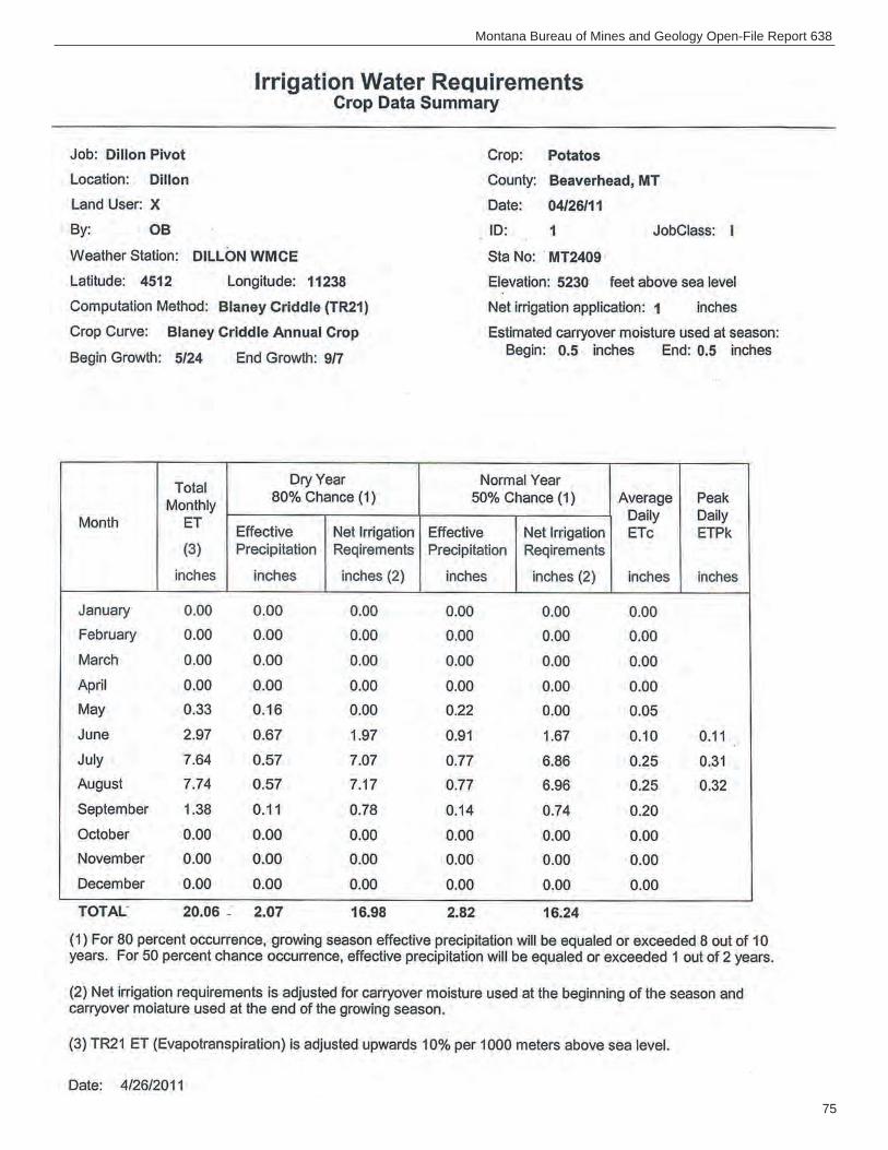
75
Montana Bureau of Mines and Geology Open-File Report 638
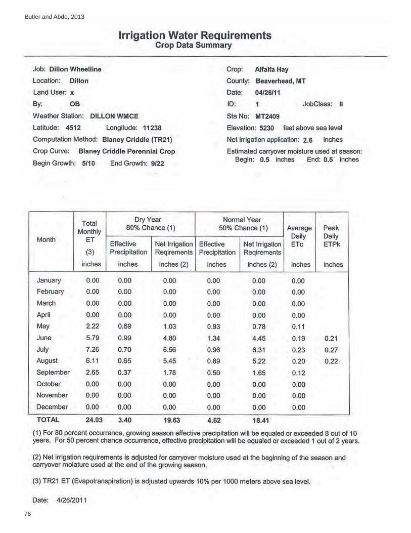
76
Butler and Abdo, 2013
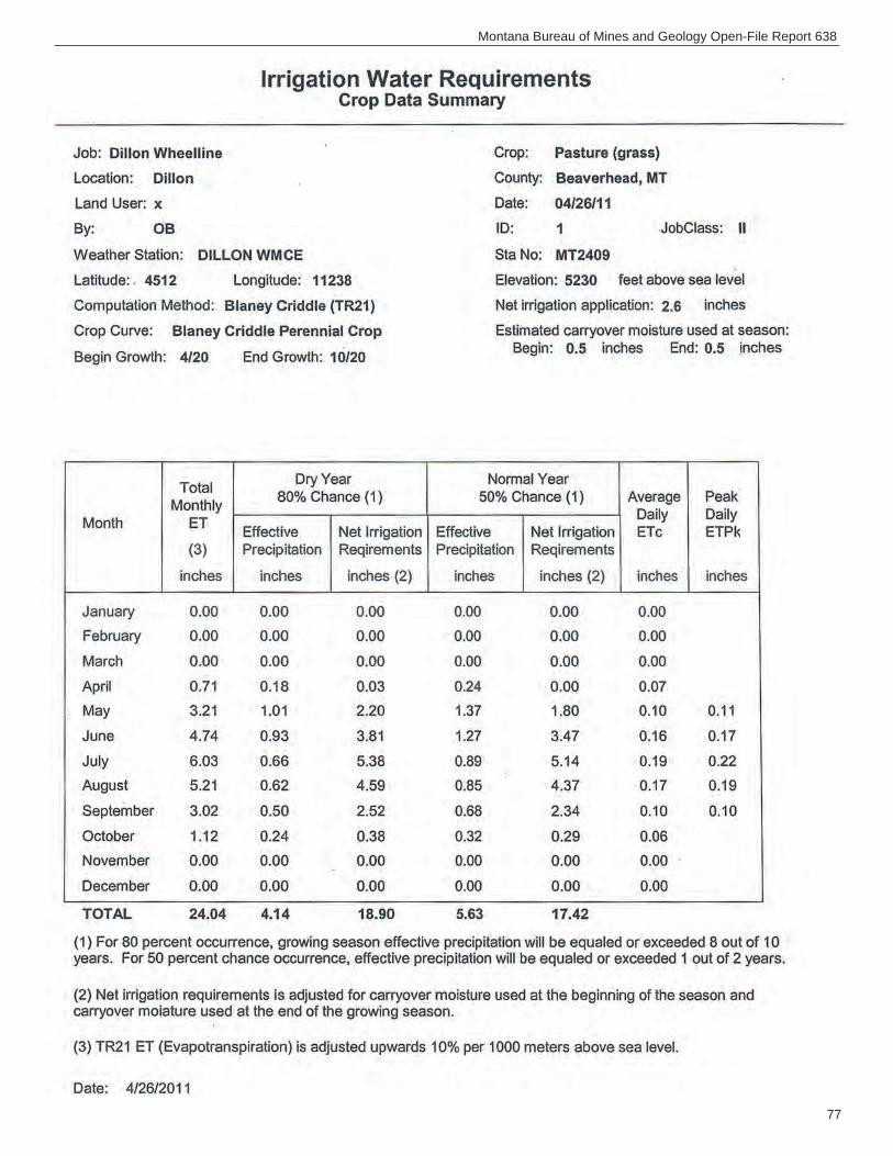
77
Montana Bureau of Mines and Geology Open-File Report 638
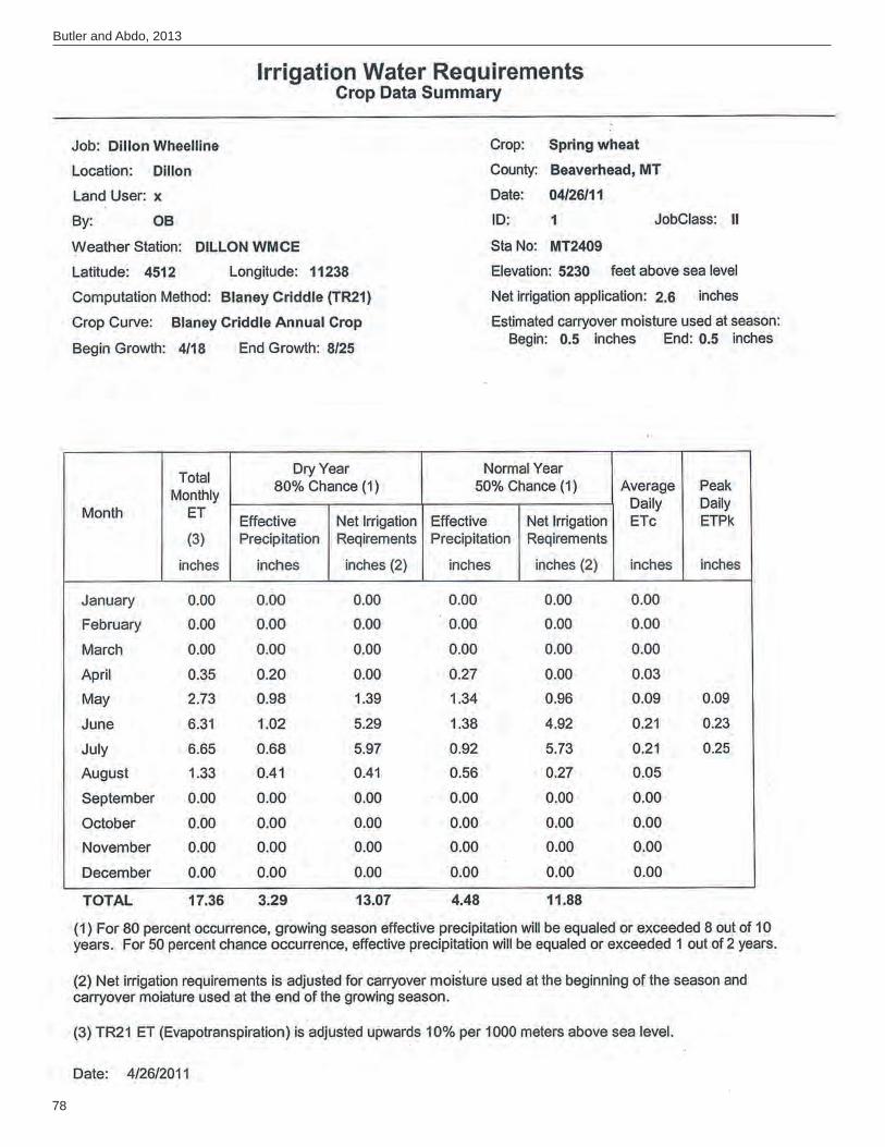
78
Butler and Abdo, 2013