Course: MBASubject: Quantitative Techniques

Unit: 4.1

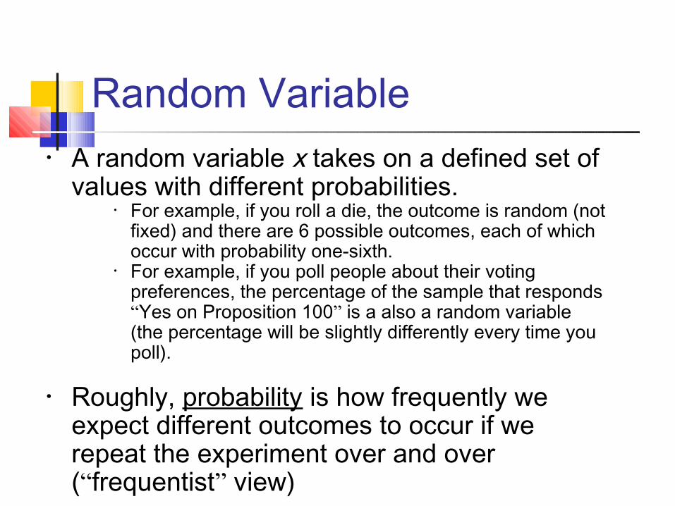
Random Variable• A random variable x takes on a defined set of

values with different probabilities.• For example, if you roll a die, the outcome is random (not

fixed) and there are 6 possible outcomes, each of which occur with probability one-sixth.

• For example, if you poll people about their voting preferences, the percentage of the sample that responds “Yes on Proposition 100” is a also a random variable (the percentage will be slightly differently every time you poll).

• Roughly, probability is how frequently we expect different outcomes to occur if we repeat the experiment over and over (“frequentist” view)

Random variables can be discrete or continuous

Discrete random variables have a countable number of outcomes Examples: Dead/alive, treatment/placebo, dice,

counts, etc. Continuous random variables have an

infinite continuum of possible values. Examples: blood pressure, weight, the speed of a

car, the real numbers from 1 to 6.

Probabil ity functions A probability function maps the possible

values of x against their respective probabilities of occurrence, p(x)

p(x) is a number from 0 to 1.0. The area under a probability function is

always 1.

Discrete example: roll of a die

x

p(x)

1/6

1 4 5 62 3

∑ = xall

1 P(x)

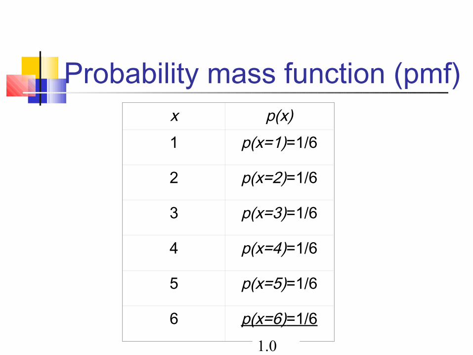
Probability mass function (pmf)x p(x)1 p(x=1)=1/6

2 p(x=2)=1/6

3 p(x=3)=1/6

4 p(x=4)=1/6

5 p(x=5)=1/6

6 p(x=6)=1/6

1.0

Cumulative distribution function (CDF)

x

P(x)

1/6

1 4 5 62 3

1/31/22/35/61.0

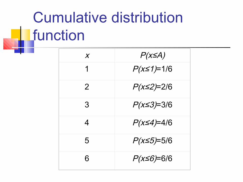
Cumulative distribution function

x P(x≤A)1 P(x≤1)=1/6

2 P(x≤2)=2/6

3 P(x≤3)=3/6

4 P(x≤4)=4/6

5 P(x≤5)=5/6

6 P(x≤6)=6/6

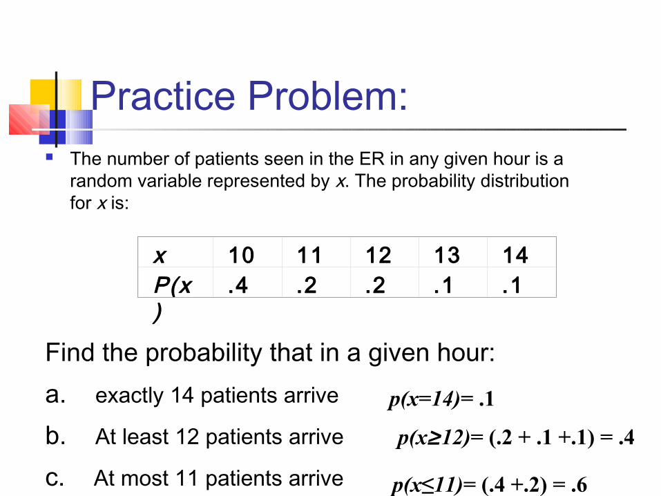
Practice Problem: The number of patients seen in the ER in any given hour is a

random variable represented by x. The probability distribution for x is:

x 10 11 12 13 14P(x)

.4 .2 .2 .1 .1

Find the probability that in a given hour:a.    exactly 14 patients arrive

b.    At least 12 patients arrive

c.    At most 11 patients arrive

 p(x=14)= .1

p(x≥12)= (.2 + .1 +.1) = .4

p(x≤11)= (.4 +.2) = .6

Review Question 1

If you toss a die, what’s the probability that you roll a 3 or less?

a. 1/6b. 1/3c. 1/2d. 5/6e. 1.0

Review Question 1

If you toss a die, what’s the probability that you roll a 3 or less?

a. 1/6b. 1/3c. 1/2d. 5/6e. 1.0

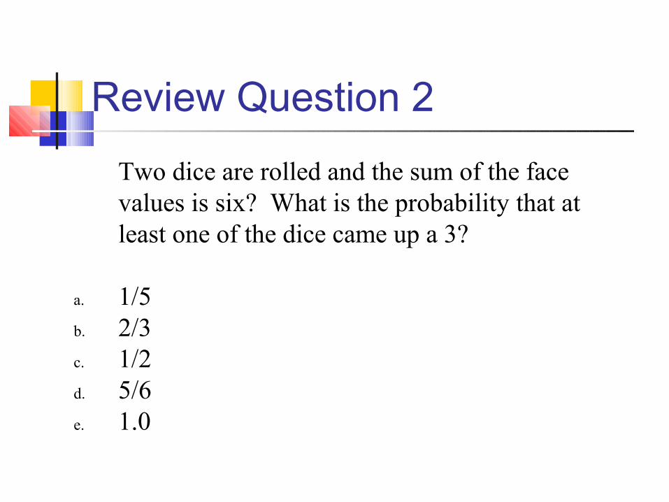
Review Question 2

Two dice are rolled and the sum of the face values is six? What is the probability that at least one of the dice came up a 3?

a. 1/5b. 2/3c. 1/2d. 5/6e. 1.0

Review Question 2

Two dice are rolled and the sum of the face values is six. What is the probability that at least one of the dice came up a 3?

a. 1/5b. 2/3c. 1/2d. 5/6e. 1.0

How can you get a 6 on two dice? 1-5, 5-1, 2-4, 4-2, 3-3

One of these f ive has a 3.

∴1/5

Continuous case The probability function that accompanies

a continuous random variable is a continuous mathematical function that integrates to 1.

For example, recall the negative exponential function (in probability, this is called an “exponential distribution”): xexf −=)(

1100

0

=+=−=+∞

−+∞

−∫ xx ee

This function integrates to 1:

Continuous case: “probability density function” (pdf)

x

p(x)=e-x

1

The probability that x is any exact particular value (such as 1.9976) is 0; we can only assign probabilities to possible ranges of x.

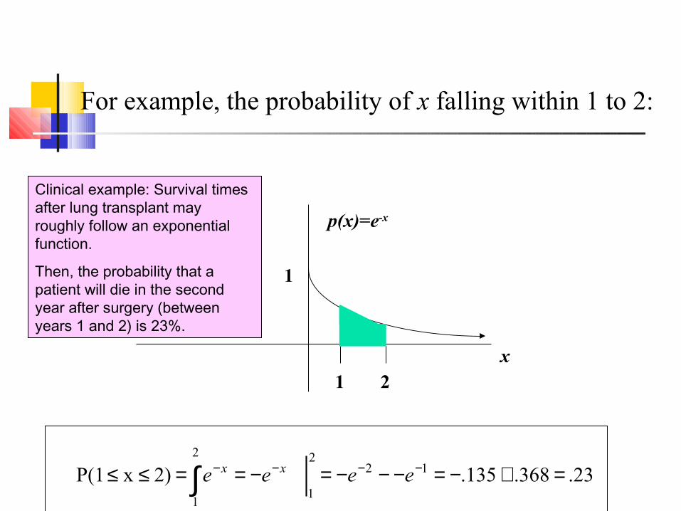
For example, the probability of x falling within 1 to 2:

23.368.135. 2)xP(1 122

1

2

1

=+−=−−−=−==≤≤ −−−−∫ eeee xx

x

p(x)=e-x

1

1 2

Clinical example: Survival times after lung transplant may roughly follow an exponential function.

Then, the probability that a patient will die in the second year after surgery (between years 1 and 2) is 23%.

Example 2: Uniform distribution

The uniform distribution: all values are equally likely.f(x)= 1 , for 1≥ x ≥0

x

p(x)

1

1

We can see it’s a probability distribution because it integrates to 1 (the area under the curve is 1):  1011

1

0

1

0

=−==∫ x

Example: Uniform distribution What’s the probability that x is between 0 and ½?

P(½ ≥x≥ 0)= ½

Clinical Research Example: When randomizing patients in an RCT, we often use a random number generator on the computer. These programs work by randomly generating a number between 0 and 1 (with equal probability of every number in between). Then a subject who gets X<.5 is control and a subject who gets X>.5 is treatment.

x

p(x)

1

1½0

Expected Value and Variance

All probability distributions are characterized by an expected value (mean) and a variance (standard deviation squared).

Expected value of a random variable

Expected value is just the average or mean (µ) of random variable x.

It’s sometimes called a “weighted average” because more frequent values of X are weighted more highly in the average.

It’s also how we expect X to behave on-average over the long run (“frequentist” view again).

Expected value, formally

∑= xall

)( )p(xxXE ii

Discrete case:

Continuous case:

dx)p(xxXE ii∫= xall

)(

Symbol Interlude E(X) = µ

these symbols are used interchangeably

Example: expected value

Recall the following probability distribution of ER arrivals:

x 10 11 12 13 14P(x)

.4 .2 .2 .1 .1

∑=

=++++=5

1

3.11)1(.14)1(.13)2(.12)2(.11)4(.10)(i

i xpx

Sample Mean is a special case of Expected Value…

Sample mean, for a sample of n subjects: =

)1

(1

1

nx

n

x

Xn

ii

n

ii

∑∑

=

= ==

The probabil i ty (frequency) of each person in the sample is 1/n.

Expected Value Expected value is an extremely useful

concept for good decision-making!

Example: the lottery The Lottery (also known as a tax on people

who are bad at math…) A certain lottery works by picking 6 numbers

from 1 to 49. It costs $1.00 to play the lottery, and if you win, you win $2 million after taxes.

If you play the lottery once, what are your expected winnings or losses?

Lottery

8-

49

6

10 x 7.2 816,983,13

1

!6!43!49

11 ===

x$ p(x)

-1 .999999928

+ 2 mil l ion 7.2 x 10 --8

Calculate the probability of winning in 1 try:

The probability function (note, sums to 1.0):

“49 choose 6”

Out of 49 numbers, this is the number of distinct combinations of 6.

Expected Valuex$ p(x)

-1 .999999928

+ 2 mil l ion 7.2 x 10 --8

The probability function

Expected Value

E(X) = P(win)*$2,000,000 + P(lose)*-$1.00 = 2.0 x 106 * 7.2 x 10-8+ .999999928 (-1) = .144 - .999999928 = -$.86  

Negative expected value is never good! You shouldn’t play if you expect to lose money!

Expected ValueIf you play the lottery every week for 10 years, what are your expected winnings or losses? 520 x (-.86) = -$447.20

Gambling (or how casinos can afford to give so many free drinks…)

A roulette wheel has the numbers 1 through 36, as well as 0 and 00. If you bet $1 that an odd number comes up, you win or lose $1 according to whether or not that event occurs. If random variable X denotes your net gain, X=1 with probability 18/38 and X= -1 with probability 20/38.

 E(X) = 1(18/38) – 1 (20/38) = -$.053 On average, the casino wins (and the player loses) 5 cents per game.  The casino rakes in even more if the stakes are higher: E(X) = 10(18/38) – 10 (20/38) = -$.53 If the cost is $10 per game, the casino wins an average of 53 cents per

game. If 10,000 games are played in a night, that’s a cool $5300.

Expected value isn’t everything though… Take the hit new show “Deal or No Deal” Everyone know the rules? Let’s say you are down to two cases left. $1

and $400,000. The banker offers you $200,000.

So, Deal or No Deal?

Deal or No Deal… This could really be represented as a

probability distribution and a non-random variable:

x$ p(x)

+1 .50

+$400,000 .50

x$ p(x)

+$200,000 1.0

Expected value doesn’t help…

x$ p(x)

+1 .50

+$400,000 .50

x$ p(x)

+$200,000 1.0

000,200)50(.000,400)50(.1)( xall

=++=== ∑ )p(xxXE iiµ

000,200)( == XEµ

How to decide?

Variance!

• If you take the deal, the variance/standard deviation is 0.

•I f you don’t take the deal, what is average deviation from the mean?

•What’s your gut guess?

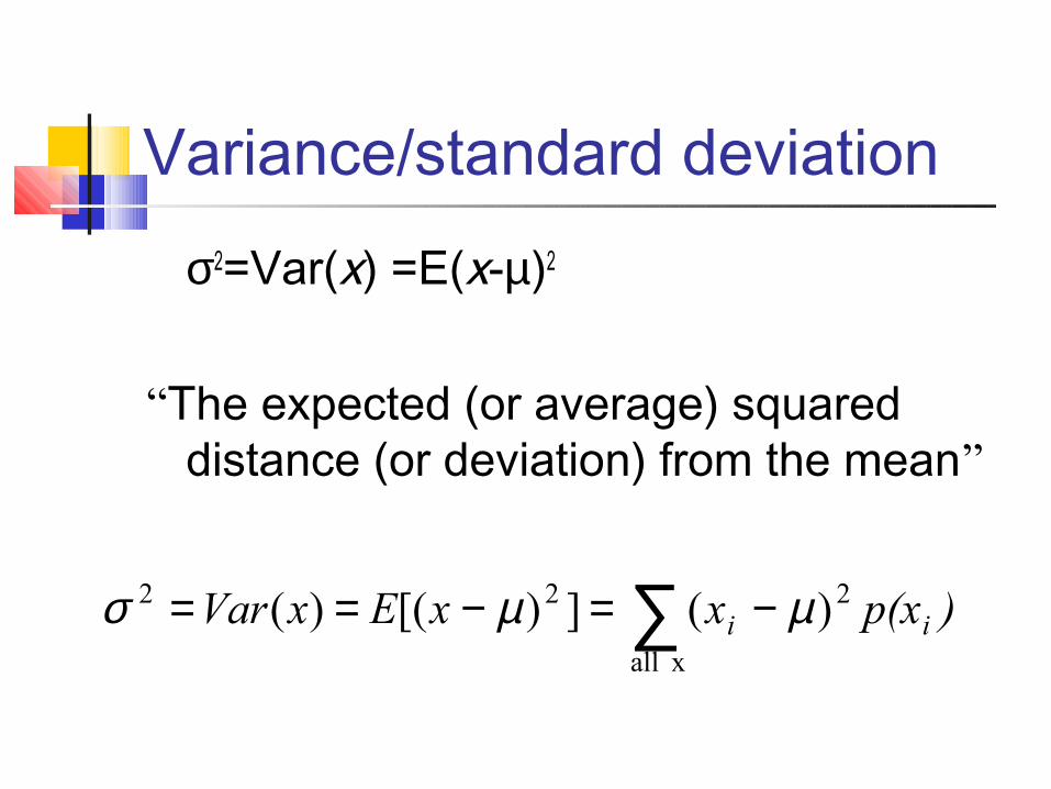
Variance/standard deviation

σ2=Var(x) =E(x-µ)2

“The expected (or average) squared distance (or deviation) from the mean”

∑ −=−== xall

222 )(])[()( )p(xxxExVar ii µµσ

Variance, continuous

∑ −= xall

2)()( )p(xxXVar ii µDiscrete case:

Continuous case?:

dx)p(xxXVar ii∫ −= xall

2)()( µ

Symbol Interlude Var(X)= σ2

SD(X) = σ these symbols are used interchangeably

Similarity to empirical variance

The variance of a sample: s2 =

)1

1()(

1

)(2

1

2

1

−−=

−

−

∑∑

=

=

nxx

n

xxN

ii

N

ii

Division by n-1 reflects the fact that we have lost a “degree of freedom” (piece of information) because we had to estimate the sample mean before we could estimate the sample variance.

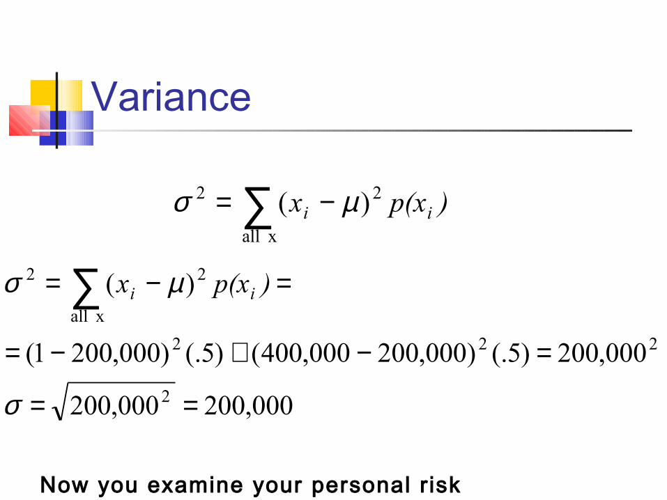
Variance

∑ −= xall

22 )( )p(xx ii µσ

000,200000,200

000,200)5(.)000,200000,400()5(.)000,2001(

)(

2

222

xall

22

==

=−+−=

=−= ∑

σ

µσ )p(xx ii

Now you examine your personal r isk tolerance…

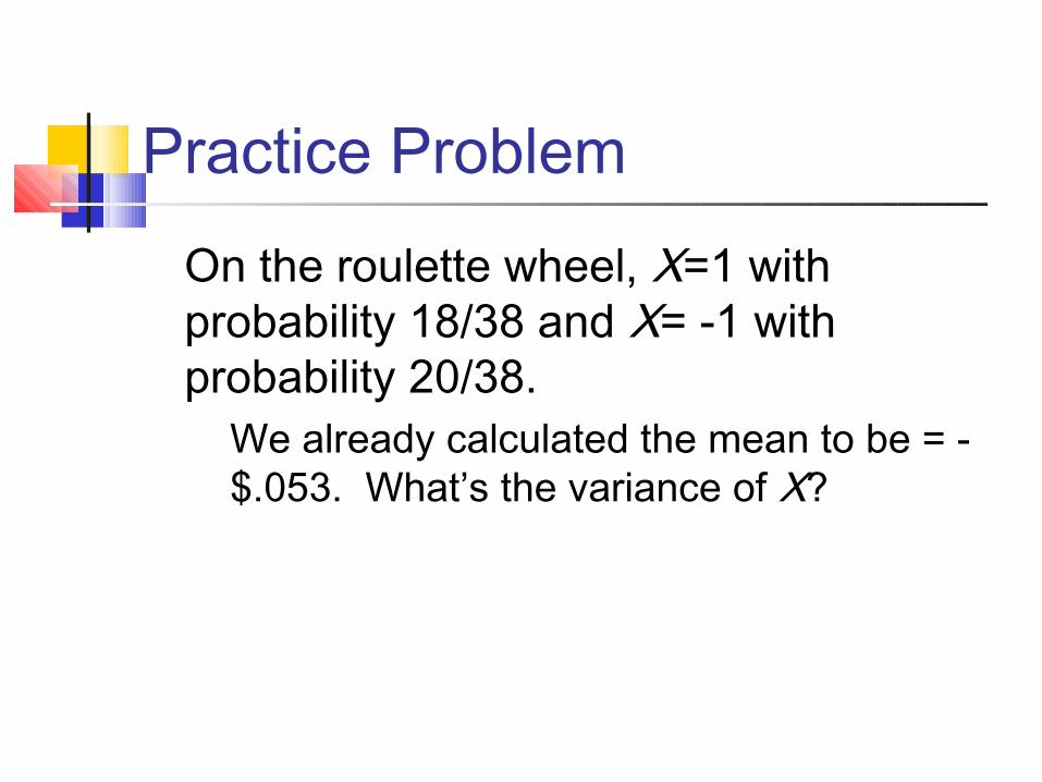
Practice Problem

On the roulette wheel, X=1 with probability 18/38 and X= -1 with probability 20/38. We already calculated the mean to be = -

$.053. What’s the variance of X?

Answer

Standard deviation is $.99. Interpretation: On average, you’re either 1 dollar above or 1 dollar below the mean, which is just under zero. Makes sense!

∑ −= xall

22 )( )p(xx ii µσ

997.

)38/20()947.()38/18()053.1(

)38/20()053.1()38/18()053.1(

)38/20()053.1()38/18()053.1(

22

22

22

=−+=

+−+=

−−−+−−+=

99.997. ==σ

Review Question 3

The expected value and variance of a coin toss (H=1, T=0) are?

a. .50, .50b. .50, .25c. .25, .50d. .25, .25

Review Question 3

The expected value and variance of a coin toss are?

a. .50, .50b. .50, .25c. .25, .50d. .25, .25

Important discrete probability distribution: The binomial

MBA SEM 3

Unit 4

Binomial Probability Distribution

A fixed number of observations (trials), n e.g., 15 tosses of a coin; 20 patients; 1000 people

surveyed A binary outcome

e.g., head or tail in each toss of a coin; disease or no disease

Generally called “success” and “failure” Probability of success is p, probability of failure is 1 – p

Constant probability for each observation e.g., Probability of getting a tail is the same each time

we toss the coin

Binomial distribution

Take the example of 5 coin tosses. What’s the probability that you flip exactly 3 heads in 5 coin tosses?

Binomial distributionSolution:One way to get exactly 3 heads: HHHTT

What’s the probability of this exact arrangement?P(heads)xP(heads) xP(heads)xP(tails)xP(tails)

=(1/2)3 x (1/2)2

Another way to get exactly 3 heads: THHHTProbability of this exact outcome = (1/2)1 x (1/2)3 x

(1/2)1 = (1/2)3 x (1/2)2

Binomial distribution

In fact, (1/2)3 x (1/2)2 is the probability of each unique outcome that has exactly 3 heads and 2 tails.

So, the overall probability of 3 heads and 2 tails is:(1/2)3 x (1/2)2 + (1/2)3 x (1/2)2 + (1/2)3 x (1/2)2 + ….. for as many unique arrangements as there are—but how many are there??

Outcome Probability THHHT (1/2)3 x (1/2)2

HHHTT (1/2)3 x (1/2)2

TTHHH (1/2)3 x (1/2)2

HTTHH (1/2)3 x (1/2)2

HHTTH (1/2)3 x (1/2)2

HTHHT (1/2)3 x (1/2)2

THTHH (1/2)3 x (1/2)2

HTHTH (1/2)3 x (1/2)2

HHTHT (1/2)3 x (1/2)2

THHTH (1/2)3 x (1/2)2

10 arrangements x (1/2)3 x (1/2)2

The probability of each unique outcome (note: they are all equal)

ways to arrange 3 heads in 5 trials

5

3

5C3 = 5!/3!2! = 10

Factorial review: n! = n(n-1)(n-2)…

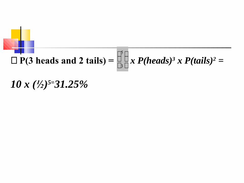
∴P(3 heads and 2 tails) = x P(heads)3 x P(tails)2 =

10 x (½)5=31.25%

5

3

x

p(x)

0 3 4 51 2

Binomial distribution function:X= the number of heads tossed in 5 coin tosses

number of heads

p(x)

number of heads

Binomial distribution, generally

XnXn

Xpp −−

)1(1-p = probability of failure

p = probability of success

X = # successes out of n trials

n = number of trials

Note the general pattern emerging if you have only two possible outcomes (call them 1/0 or yes/no or success/failure) in n independent trials, then the probability of exactly X “successes”=

Binomial distribution: example

If I toss a coin 20 times, what’s the probability of getting exactly 10 heads?

176.)5(.)5(. 101020

10=

Binomial distribution: example If I toss a coin 20 times, what’s the

probability of getting of getting 2 or fewer heads?

4

472018220

2

572019120

1

72020020

0

108.1

108.1105.9190)5(.!2!18

!20)5(.)5(.

109.1105.920)5(.!1!19

!20)5(.)5(.

105.9)5(.!0!20

!20)5(.)5(.

−

−−

−−

−

=

===

+===

+==

x

xxx

xxx

x

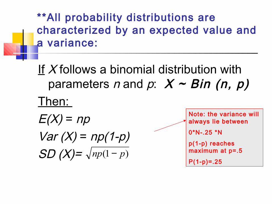
**All probabil i ty distributions are characterized by an expected value and a variance:

If X follows a binomial distribution with parameters n and p: X ~ Bin (n, p)

Then: E(X) = npVar (X) = np(1-p)SD (X)= )1( pnp −

Note: the variance wil l always l ie between

0*N-.25 *N

p(1-p) reaches maximum at p=.5

P(1-p)=.25

Practice Problem 1. You are performing a cohort study. If the

probability of developing disease in the exposed group is .05 for the study duration, then if you (randomly) sample 500 exposed people, how many do you expect to develop the disease? Give a margin of error (+/- 1 standard deviation) for your estimate.

2. What’s the probability that at most 10 exposed people develop the disease?

Answer1. How many do you expect to develop the disease? Give a margin of

error (+/- 1 standard deviation) for your estimate.

X ~ binomial (500, .05)

E(X) = 500 (.05) = 25

Var(X) = 500 (.05) (.95) = 23.75

StdDev(X) = square root (23.75) = 4.87 

∴25 ± 4.87

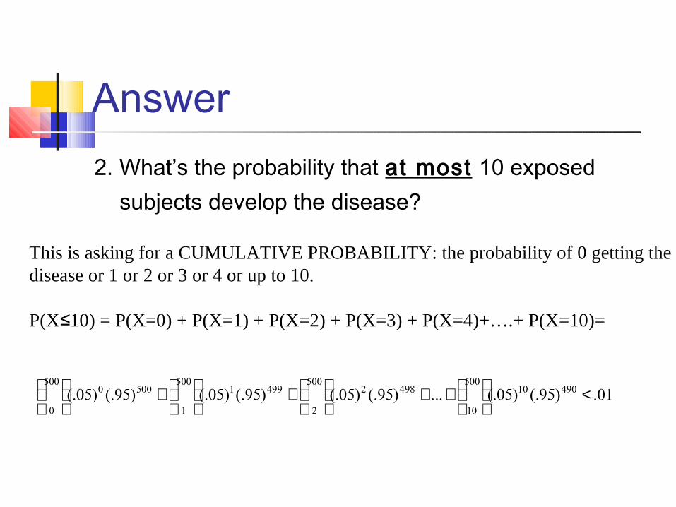
Answer2. What’s the probability that at most 10 exposed

subjects develop the disease?

01.)95(.)05(....)95(.)05(.)95(.)05(.)95(.)05(. 49010500

10

4982500

2

4991500

1

5000500

0<

++

+

+

This is asking for a CUMULATIVE PROBABILITY: the probability of 0 getting the disease or 1 or 2 or 3 or 4 or up to 10. P(X 10) = P(X=0) + P(X=1) + P(X=2) + P(X=3) + P(X=4)+….+ P(X=10)=≤

Practice Problem:You are conducting a case-control study of smoking and lung cancer. If the probability of being a smoker among lung cancer cases is .6, what’s the probability that in a group of 8 cases you have:

a. Less than 2 smokers? b. More than 5?c. What are the expected value and variance of the number

of smokers?

Answer

1 4 52 3 6 7 80

X P(X) 0 1(.4)

8=.00065 1 8(.6)

1 (.4)

7 =.008 2 28(.6)

2 (.4)

6 =.04 3 56(.6)

3 (.4)

5 =.12 4 70(.6)

4 (.4)

4 =.23 5 56(.6)

5 (.4)

3 =.28 6 28(.6)

6 (.4)

2 =.21 7 8(.6)

7 (.4)

1=.090 8 1(.6)

8 =.0168

Answer, continued

1 4 52 3 6 7 80

E(X) = 8 (.6) = 4.8Var(X) = 8 (.6) (.4) =1.92StdDev(X) = 1.38

P(<2)=.00065 + .008 = .00865 P(>5)=.21+.09+.0168 = .3168

Review Question 4In your case-control study of smoking and lung-cancer, 60% of cases are smokers versus only 10% of controls. What is the odds ratio between smoking and lung cancer?

a. 2.5 b. 13.5c. 15.0d. 6.0e. .05

Review Question 4In your case-control study of smoking and lung-cancer, 60% of cases are smokers versus only 10% of controls. What is the odds ratio between smoking and lung cancer?

a. 2.5 b. 13.5c. 15.0d. 6.0e. .05

5.132

27

1

9

2

3

9.

1.4.

6.

=== x

Review Question 5What’s the probability of getting exactly 5 heads in 10 coin tosses?

a. b. c. d.

5510

0)50(.)50(.

5510

5)50(.)50(.

51010

5)50(.)50(.

01010

10)50(.)50(.

Review Question 5What’s the probability of getting exactly 5 heads in 10 coin tosses?

a. b. c. d.

5510

0)50(.)50(.

5510

5)50(.)50(.

51010

5)50(.)50(.

01010

10)50(.)50(.

Review Question 6A coin toss can be thought of as an example of a binomial distribution with N=1 and p=.5. What are the expected value and variance of a coin toss?

a. .5, .25b. 1.0, 1.0c. 1.5, .5d. .25, .5e. .5, .5

Review Question 6A coin toss can be thought of as an example of a binomial distribution with N=1 and p=.5. What are the expected value and variance of a coin toss?

a. .5, .25b. 1.0, 1.0c. 1.5, .5d. .25, .5e. .5, .5

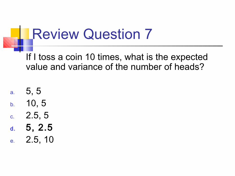
Review Question 7If I toss a coin 10 times, what is the expected value and variance of the number of heads?

a. 5, 5b. 10, 5c. 2.5, 5d. 5, 2.5e. 2.5, 10

Review Question 7If I toss a coin 10 times, what is the expected value and variance of the number of heads?

a. 5, 5b. 10, 5c. 2.5, 5d. 5, 2.5e. 2.5, 10

Review Question 8In a randomized trial with n=150, the goal is to randomize half to treatment and half to control. The number of people randomized to treatment is a random variable X. What is the probability distribution of X?

a. X~Normal(µ=75,σ=10)b. X~Exponential(µ=75)c. X~Uniformd. X~Binomial(N=150, p=.5)e. X~Binomial(N=75, p=.5)

Review Question 8In a randomized trial with n=150, every subject has a 50% chance of being randomized to treatment. The number of people randomized to treatment is a random variable X. What is the probability distribution of X?

a. X~Normal(µ=75,σ=10)b. X~Exponential(µ=75)c. X~Uniformd. X~Binomial(N=150, p=.5)e. X~Binomial(N=75, p=.5)

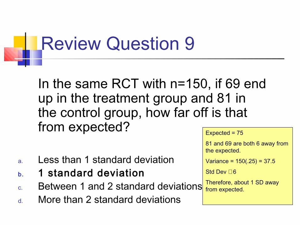
Review Question 9

In the same RCT with n=150, if 69 end up in the treatment group and 81 in the control group, how far off is that from expected?

a. Less than 1 standard deviationb. 1 standard deviationc. Between 1 and 2 standard deviationsd. More than 2 standard deviations

Review Question 9

In the same RCT with n=150, if 69 end up in the treatment group and 81 in the control group, how far off is that from expected?

a. Less than 1 standard deviationb. 1 standard deviationc. Between 1 and 2 standard deviationsd. More than 2 standard deviations

Expected = 75

81 and 69 are both 6 away from the expected.

Variance = 150(.25) = 37.5

Std Dev ≅ 6

Therefore, about 1 SD away from expected.

Proportions… The binomial distribution forms the basis of

statistics for proportions. A proportion is just a binomial count divided

by n. For example, if we sample 200 cases and find 60

smokers, X=60 but the observed proportion=.30. Statistics for proportions are similar to

binomial counts, but differ by a factor of n.

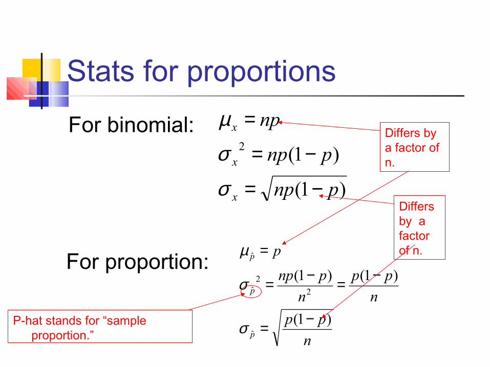
Stats for proportions

For binomial:

)1(

)1(2

pnp

pnp

np

x

x

x

−=

−=

=

σ

σ

µ

For proportion:

n

pp

n

pp

n

pnp

p

p

p

p

)1(

)1()1(

ˆ

2

2ˆ

ˆ

−=

−=−=

=

σ

σ

µ

P-hat stands for “sample proportion.”

Differs by a factor of n.

Differs by a factor of n.

It all comes back to normal… Statistics for proportions are based on a

normal distribution, because the binomial can be approximated as normal if np>5

References Quantitative Techniques, by CR

Kothari, Vikas publication Fundamentals of Statistics by SC Guta

Publisher Sultan Chand                Quantitative Techniques in

management by N.D. Vohra Publisher: Tata Mcgraw hill