Maxwell 2D Student Version - Lily · PDF fileMaxwell® 2D Student Version A 2D...
84
Maxwell ® 2D Student Version A 2D Magnetostatic Problem November 2002
Transcript of Maxwell 2D Student Version - Lily · PDF fileMaxwell® 2D Student Version A 2D...

Maxwell® 2D Student Version
�
A 2D Magnetostatic Problem
November 2002

NoticeThe information contained in this document is subject to change without notice.Ansoft makes no warranty of any kind with regard to this material, including, but not limited to, the implied warranties of merchantability and fitness for a particular purpose. Ansoft shall not be liable for errors contained herein or for incidental or consequential damages in connection with the fur-nishing, performance, or use of this material.This document contains proprietary information which is protected by copyright. All rights are reserved.
Ansoft CorporationFour Station Square�Suite 200�Pittsburgh, PA 15219�(412) 261 - 3200
Microsoft® Windows® is a registered trademark of Microsoft Corporation.UNIX� is a registered trademark of UNIX Systems Laboratories, Inc.Maxwell� is a registered trademark of Ansoft Corporation.
© Copyright 1993-2002 Ansoft Corporation

Getting Started: A 2D Magnetostatic Problem
Printing HistoryNew editions of this manual incorporate all material updated since the previous edition. The man-ual printing date, which indicates the manual’s current edition, changes when a new edition is printed. Minor corrections and updates which are incorporated at reprint do not cause the date to change.Update packages, which may contain additional and/or replacement pages for you to merge into the manual, may be issued between editions. Pages that are rearranged due to changes on a previous page are not considered to be revised.
Edition Date Software Revision
1 May 2001 8.1
2 November 2002 9.0
iii

Getting Started: A 2D Magnetostatic Problem
InstallationBefore you use Maxwell SV, you must:1. Set up your system’s graphical windowing system.2. Install the Ansoft software, using the directions in the Ansoft PC Installation Guide.If you have not yet done these steps, refer to the Ansoft installation guides and the documentation that came with your computer system, or ask your system administrator for assistance.
Getting StartedIf you are using Maxwell SV for the first time, the following two guides are available for the Stu-dent Version of Maxwell 2D:• Getting Started: A 2D Electrostatic Problem• Getting Started: A 2D Magnetostatic ProblemAdditional Getting Started guides are available for the standard version of Maxwell 2D.These short tutorials guide you through the process of setting up and solving simple problems in Maxwell SV, providing you with an overview of how to use the software.
Other ReferencesTo start Maxwell SV, you must first access the Maxwell Control Panel.For information on all Maxwell Control Panel and Maxwell SV commands, refer to the following online documentation:
• Maxwell Control Panel online help. The Control panel online help contains a detailed description of all of the commands in the Maxwell Control Panel and in the Utilities Panel. The Maxwell Control Panel allows you to create and open projects, print screens, and translate files. The Utilities Panel is accessible through the Maxwell Control Panel and enables you to view licensing information, adjust colors, open and create 2D models, open and create plots using parametric equations, and evaluate mathematical expressions.
• Maxwell 2D online help. The Maxwell 2D online help contains a detailed description of the Maxwell 2D software and the Parametric Analysis module. Maxwell SV does not pro-vide parametric capabilities.
iv

Getting Started: A 2D Magnetostatic Problem
Typeface ConventionsField Names Bold type is used for on-screen prompts, field names, and messages.
Keyboard Entries Bold type is used for entries that must be entered as specified. Example: Enter 0.005 in the Nonlinear Residual field.
Menu Commands Bold type is used to display menu commands selected to perform a specific task. Menu levels are separated by a carat.Example 1: The instruction “Click File>Open” means to select the Open command on the File menu within an application.Example 2: The instruction “Click Define Model>Draw Model” means to select the Draw Model command from the Define Model button on the Maxwell SV Executive Commands menu.
Variable Names Italic type is used for keyboard entries when a name or variable must be typed in place of the words in italics. Example: The instruction “copy filename” means to type the word copy, to type a space, and then to type the name of a file, such as file1.
Emphasis and Titles
Italic type is used for emphasis and for the titles of manuals and other publications.
Keyboard Keys Bold type, in Arial font, is used for labeled keys on the computer keyboard. Example: The instruction “Press Return” means to press the key on the computer that is labeled Return.
v

Getting Started: A 2D Magnetostatic Problem
vi

Table of Contents
1. Introduction . . . . . . . . . . . . . . . . . . . . . . . . . . . . . . . . . . 1-1The Sample Problem . . . . . . . . . . . . . . . . . . . . . . . . . . . . . . . . . . . . . . . . . 1-2General Procedure for Creating and Solving a 2D Model . . . . . . . . . . . . . 1-3Goals . . . . . . . . . . . . . . . . . . . . . . . . . . . . . . . . . . . . . . . . . . . . . . . . . . . . . 1-5
2. Creating the Project . . . . . . . . . . . . . . . . . . . . . . . . . . . 2-1Access the Control Panel . . . . . . . . . . . . . . . . . . . . . . . . . . . . . . . . . . . . . . 2-2Start the Project Manager . . . . . . . . . . . . . . . . . . . . . . . . . . . . . . . . . . . . . 2-2Create a Project Directory . . . . . . . . . . . . . . . . . . . . . . . . . . . . . . . . . . . . 2-3Create a New Project . . . . . . . . . . . . . . . . . . . . . . . . . . . . . . . . . . . . . . . . . 2-4
Access the Project Directory . . . . . . . . . . . . . . . . . . . . . . . . . . . . . . . . . . 2-4Add the New Project . . . . . . . . . . . . . . . . . . . . . . . . . . . . . . . . . . . . . . . . 2-4Save Project Notes . . . . . . . . . . . . . . . . . . . . . . . . . . . . . . . . . . . . . . . . . . 2-5
Open the New Project and Run Maxwell SV . . . . . . . . . . . . . . . . . . . . . . 2-6Overview of the Executive Commands Window . . . . . . . . . . . . . . . . . . . 2-7
Executive Commands Menu . . . . . . . . . . . . . . . . . . . . . . . . . . . . . . . . . . 2-7Display Area . . . . . . . . . . . . . . . . . . . . . . . . . . . . . . . . . . . . . . . . . . . . . . 2-7
3. Creating the Model . . . . . . . . . . . . . . . . . . . . . . . . . . . . 3-1Define Model Type . . . . . . . . . . . . . . . . . . . . . . . . . . . . . . . . . . . . . . . . . . 3-2
Select the Solver Type . . . . . . . . . . . . . . . . . . . . . . . . . . . . . . . . . . . . . . . 3-2Define the Drawing Plane . . . . . . . . . . . . . . . . . . . . . . . . . . . . . . . . . . . . 3-2
Access the 2D Modeler . . . . . . . . . . . . . . . . . . . . . . . . . . . . . . . . . . . . . . . 3-3Screen Layout . . . . . . . . . . . . . . . . . . . . . . . . . . . . . . . . . . . . . . . . . . . . . 3-3
The Solenoid Model . . . . . . . . . . . . . . . . . . . . . . . . . . . . . . . . . . . . . . . . . . 3-5
Contents-1

Getting Started: A 2D Magnetostatic Problem
Set Up the Drawing Region . . . . . . . . . . . . . . . . . . . . . . . . . . . . . . . . . . . . 3-6Change the Drawing Size . . . . . . . . . . . . . . . . . . . . . . . . . . . . . . . . . . . . . 3-7Change Grid Spacing . . . . . . . . . . . . . . . . . . . . . . . . . . . . . . . . . . . . . . . . . 3-8Create the Geometry . . . . . . . . . . . . . . . . . . . . . . . . . . . . . . . . . . . . . . . . . 3-9Draw the Plugnut . . . . . . . . . . . . . . . . . . . . . . . . . . . . . . . . . . . . . . . . . . . . 3-9
Create a Rectangle . . . . . . . . . . . . . . . . . . . . . . . . . . . . . . . . . . . . . . . . . . 3-9Change the Plugnut’s Name and Color . . . . . . . . . . . . . . . . . . . . . . . . . . 3-10
Keyboard Entry . . . . . . . . . . . . . . . . . . . . . . . . . . . . . . . . . . . . . . . . . . . . . 3-10Draw the Core . . . . . . . . . . . . . . . . . . . . . . . . . . . . . . . . . . . . . . . . . . . . . . 3-11Draw the Coil . . . . . . . . . . . . . . . . . . . . . . . . . . . . . . . . . . . . . . . . . . . . . . . 3-12Save the Geometry . . . . . . . . . . . . . . . . . . . . . . . . . . . . . . . . . . . . . . . . . . 3-13Draw the Yoke . . . . . . . . . . . . . . . . . . . . . . . . . . . . . . . . . . . . . . . . . . . . . . 3-13Draw the Bonnet . . . . . . . . . . . . . . . . . . . . . . . . . . . . . . . . . . . . . . . . . . . . 3-14Completed Geometry . . . . . . . . . . . . . . . . . . . . . . . . . . . . . . . . . . . . . . . . . 3-14Exit the 2D Modeler . . . . . . . . . . . . . . . . . . . . . . . . . . . . . . . . . . . . . . . . . 3-15
4. Setting Up the Model . . . . . . . . . . . . . . . . . . . . . . . . . . . 4-1Assign Materials to Objects . . . . . . . . . . . . . . . . . . . . . . . . . . . . . . . . . . . 4-2
Access Material Manager . . . . . . . . . . . . . . . . . . . . . . . . . . . . . . . . . . . . . 4-2Assign Copper to the Coil . . . . . . . . . . . . . . . . . . . . . . . . . . . . . . . . . . . . 4-3Assign Cold Rolled Steel to the Bonnet and Yoke . . . . . . . . . . . . . . . . . 4-3Assign Neo35 to the Core . . . . . . . . . . . . . . . . . . . . . . . . . . . . . . . . . . . . 4-7Assign SS430 to the Plugnut . . . . . . . . . . . . . . . . . . . . . . . . . . . . . . . . . . 4-10Accept Default Material for Background . . . . . . . . . . . . . . . . . . . . . . . . . 4-12Exit the Material Manager . . . . . . . . . . . . . . . . . . . . . . . . . . . . . . . . . . . . 4-12
Set Up Boundaries and Current Sources . . . . . . . . . . . . . . . . . . . . . . . . . . 4-12Access the 2D Boundary/Source Manager . . . . . . . . . . . . . . . . . . . . . . . 4-13Boundary Manager Screen Layout . . . . . . . . . . . . . . . . . . . . . . . . . . . . . 4-13Types of Boundary Conditions and Sources . . . . . . . . . . . . . . . . . . . . . . 4-14Set Source Current on the Coil . . . . . . . . . . . . . . . . . . . . . . . . . . . . . . . . 4-14Assign Balloon Boundary to the Background . . . . . . . . . . . . . . . . . . . . . 4-15Exit the Boundary Manager . . . . . . . . . . . . . . . . . . . . . . . . . . . . . . . . . . . 4-16
Set Up Force Computation . . . . . . . . . . . . . . . . . . . . . . . . . . . . . . . . . . . . 4-165. Generating a Solution . . . . . . . . . . . . . . . . . . . . . . . . . . 5-1
View Solution Criteria . . . . . . . . . . . . . . . . . . . . . . . . . . . . . . . . . . . . . . . . 5-2Starting Mesh . . . . . . . . . . . . . . . . . . . . . . . . . . . . . . . . . . . . . . . . . . . . . . 5-2Manual Mesh . . . . . . . . . . . . . . . . . . . . . . . . . . . . . . . . . . . . . . . . . . . . . . 5-2Solver Choice . . . . . . . . . . . . . . . . . . . . . . . . . . . . . . . . . . . . . . . . . . . . . . 5-3Solver Residual . . . . . . . . . . . . . . . . . . . . . . . . . . . . . . . . . . . . . . . . . . . . 5-3
Contents-2

Getting Started: A 2D Magnetostatic Problem
Solve for Fields and Parameters . . . . . . . . . . . . . . . . . . . . . . . . . . . . . . . . 5-3Adaptive Analysis . . . . . . . . . . . . . . . . . . . . . . . . . . . . . . . . . . . . . . . . . . 5-3Exit Setup Solution Options . . . . . . . . . . . . . . . . . . . . . . . . . . . . . . . . . . . 5-3
Start the Solution . . . . . . . . . . . . . . . . . . . . . . . . . . . . . . . . . . . . . . . . . . . 5-4Monitoring the Solution . . . . . . . . . . . . . . . . . . . . . . . . . . . . . . . . . . . . . . . 5-4Viewing Convergence Data . . . . . . . . . . . . . . . . . . . . . . . . . . . . . . . . . . . . 5-5
Solution Criteria . . . . . . . . . . . . . . . . . . . . . . . . . . . . . . . . . . . . . . . . . . . . 5-5Completed Solutions . . . . . . . . . . . . . . . . . . . . . . . . . . . . . . . . . . . . . . . . 5-6
Completing the Solution Process . . . . . . . . . . . . . . . . . . . . . . . . . . . . . . . . 5-6Viewing Final Convergence Data . . . . . . . . . . . . . . . . . . . . . . . . . . . . . . . 5-7
Plotting Convergence Data . . . . . . . . . . . . . . . . . . . . . . . . . . . . . . . . . . . 5-8Viewing Statistics . . . . . . . . . . . . . . . . . . . . . . . . . . . . . . . . . . . . . . . . . . 5-9
6. Analyzing the Solution . . . . . . . . . . . . . . . . . . . . . . . . . 6-1View Force Solution . . . . . . . . . . . . . . . . . . . . . . . . . . . . . . . . . . . . . . . . . 6-2Access the Post Processor . . . . . . . . . . . . . . . . . . . . . . . . . . . . . . . . . . . . . 6-2Post Processor Screen Layout . . . . . . . . . . . . . . . . . . . . . . . . . . . . . . . . . . 6-3
General Areas . . . . . . . . . . . . . . . . . . . . . . . . . . . . . . . . . . . . . . . . . . . . . 6-3Plot the Magnetic Field . . . . . . . . . . . . . . . . . . . . . . . . . . . . . . . . . . . . . . . 6-3
Redisplay the Magnetic FIeld Plot . . . . . . . . . . . . . . . . . . . . . . . . . . . . . . 6-5Identify Saturated Materials . . . . . . . . . . . . . . . . . . . . . . . . . . . . . . . . . . . 6-6
Plot Magnetic Flux Density . . . . . . . . . . . . . . . . . . . . . . . . . . . . . . . . . . . 6-6Plot the B-H Curve . . . . . . . . . . . . . . . . . . . . . . . . . . . . . . . . . . . . . . . . . . 6-8
Exit the Post Processor . . . . . . . . . . . . . . . . . . . . . . . . . . . . . . . . . . . . . . . 6-9Exit Maxwell SV . . . . . . . . . . . . . . . . . . . . . . . . . . . . . . . . . . . . . . . . . . . . 6-9Exit the Maxwell Software . . . . . . . . . . . . . . . . . . . . . . . . . . . . . . . . . . . . 6-9
Contents-3

Getting Started: A 2D Magnetostatic Problem
Contents-4

Introduction
This guide is a tutorial for setting up a magnetostatic problem using version 9.0 of Maxwell 2D Stu-dent Version (SV), a software package for analyzing electromagnetic fields in cross-sections of structures. Maxwell SV uses finite element analysis (FEA) to solve two-dimensional (2D) electro-magnetic problems. To analyze a problem, you need to specify the appropriate geometry, material properties, and exci-tations for a device or system of devices. The Maxwell software then does the following:
• Automatically creates the required finite element mesh.• Calculates the desired electric or magnetic field solution and special quantities of interest,
such as force, torque, inductance, capacitance, or power loss. You can select any of the following solution types: Electrostatic, Magnetostatic, Electrostatic, Eddy Current, DC Conduction, AC Conduction, Eddy Axial. The student version does not contain thermal, transient, or parametric capabilities.
• Allows you to analyze, manipulate, and display field solutions.Many models are actually a collection of three-dimensional (3D) objects. Maxwell SV analyzes a 2D cross-section of the model, then generates a solution for that cross-section, using FEA to solve the problem. Dividing a structure into many smaller regions (finite elements) allows the system to compute the field solution separately in each element. The smaller the elements, the more accurate the final solution.
Introduction 1-1

Getting Started: A 2D Magnetostatic Problem
The Sample ProblemThe sample problem, shown below, is a solenoid that consists of the following objects:
• Core• Bonnet• Coil• Yoke• Plugnut
The 2D diagram above actually represents a 3D structure that has been revolved around an axis of symmetry, as shown in the figure below. In this figure, part of the 3D model has been cut away so that you can see the interior of the solenoid.
Since the cross-section of the solenoid is constant, it can be modeled as an axisymmetric model in Maxwell SV.
CORE
BONNET
YOKE
BACKGROUND
PLUGNUT
COIL
1-2 Introduction

Getting Started: A 2D Magnetostatic Problem
General Procedure for Creating and Solving a 2D ModelThe general procedure to follow when using the software to create and solve a 2D problem is given below:1. Use the Solver command to specify which of the following electric or magnetic field quantities
to compute:• Electrostatic • Magnetostatic • Eddy Current • DC Conduction • AC Conduction • Eddy Axial
2. Use the Drawing command to select one of the following model planes:
3. Use the Define Model commands to create the geometric model. When you click Define Model, the following menu appears:
4. Use the Setup Materials command to assign materials to all objects in the geometric model.5. Use the Setup Boundaries/Sources command to define the boundaries and sources for the
problem. This determines the electromagnetic excitations and field behavior for the model.6. Use the Setup Executive Parameters command to instruct the simulator to compute one or
more of the following special quantities during the solution process:• Matrix (capacitance, inductance, admittance, impedance, or conductance matrix, depend-
ing on the selected solver).• Force• Torque• Flux lines• Post Processor macros• Core loss • Current flow
7. Use the Setup Solution Options command to enter parameters that affect how the solution is computed.
XY Plane Cartesian models appear to sweep perpendicularly to the cross-section.RZ Plane Axisymmetric models appear to revolve around an axis of symmetry in the
cross-section.
Draw Model Allows you to access the 2D Modeler and build the objects that make up the geometric model.
Group ObjectsAllows you to group discrete objects that are actually one electrical object. For instance, two terminations of a conductor that are drawn as separate objects in the cross-section can be grouped to represent one conductor.
Introduction 1-3

Getting Started: A 2D Magnetostatic Problem
8. Use the Solve command to solve for the appropriate field quantities.9. Use the Post Process command to analyze the solution. These commands must be chosen in the sequence in which they appear. You must first create a geo-metric model using the Define Model command before you specify material characteristics for objects using the Setup Materials command. A check mark appears on the menu next to each step which has been completed.
Select solver and drawing plane.
Draw geometric model and
Assign material properties.
Assign boundary conditions and sources.
Yes
No
Set up solution criteria and
Generate solution.
Inspect parameter solutions; view
Compute other quantities during
solution?
(optionally) refine the mesh.
solution information; display plots of fields and manipulate basic field
quantities.
(optionally) identify grouped objects.
Request that force, torque, capacitance, inductance, admittance, impedance, flux linkage, core loss, conductance, or current flow be computed during the solution process.
1-4 Introduction

Getting Started: A 2D Magnetostatic Problem
GoalsThe goals in Getting Started: A 2D Magnetostatic Problem are as follows:• Determine the force on the core due to the source current in the coil.• Determine whether any of the nonlinear materials reach their saturation point.Do the following to accomplish these goals:1. Draw the plugnut, core, coil, yoke, and bonnet using the Draw Model command under Define
Model. 2. Define materials using the Setup Materials command.3. Define boundary conditions and current sources using the Setup Boundaries/Sources com-
mand.4. Request that the force on the core be computed, using the Setup Executive Parameters com-
mand.5. Specify solution criteria and generate a solution using the Setup Solution Parameters and
Solve commands. You will compute both a magnetostatic field solution and the force on the core.
6. View the results of the force computation, using the Solutions>Force command.7. Plot saturation levels and contours of equal magnetic potential via the Post Process command.This simple problem illustrates the most commonly used features of Maxwell SV.
Time This guide should take approximately 3 hours to work through.
Introduction 1-5

Getting Started: A 2D Magnetostatic Problem
1-6 Introduction

Creating the Project
This guide assumes that Maxwell SV has already been installed as described in the Ansoft PC Installation Guide. The goals for this chapter are to:
• Create a project directory in which to save sample problems.• Create a new project in that directory in which to save the solenoid problem.• Open the project and run Maxwell SV.
This chapter also includes a description of the sample problem and your goals for solving it.
Time This chapter should take approximately 15 minutes to work through.
Creating the Project 2-1

Getting Started: A 2D Magnetostatic Problem
Access the Control PanelThe Maxwell Control Panel allows you to create and open projects and directly access program modules shared by Ansoft products. You must start the Control Panel in order to start Maxwell SV.To start the Maxwell Control Panel, do one of the following:• Use the Start menu to select Programs>Ansoft>Maxwell SV. • Double-click the Maxwell SV icon.The Maxwell Control Panel appears.
If the Maxwell Control Panel does not appear, see the Ansoft installation guides for possible rea-sons. See the online help on the Maxwell Control Panel for a detailed description of other control panel options.
Start the Project ManagerUse the Project Manager to create, rename, or delete project files and to access projects created with other Ansoft products.To display the Project Manager, click PROJECTS in the Maxwell Control Panel. The Project Manager appears.
2-2 Creating the Project

Getting Started: A 2D Magnetostatic Problem
Create a Project Directory A project directory contains a specific set of projects created with Ansoft software. You can use project directories to categorize projects. For example, you might want to store all projects related to a particular application in one project directory. You will add the getting_started_SV directory for the Maxwell project you create using this Getting Started guide.
To add a project directory, do the following in the Project Manager:1. Click Add from the Project Directories area at the lower-left corner of the window. The Add
a new project directory window appears, listing the directories and subdirectories.
2. Type the following in the Alias field:getting_started_SV
Maxwell SV projects are usually created in directories which have aliases — that is, directories that have been identified as project directories using the Add command.
3. Select Make New Directory near the bottom of the window. The name you entered as the alias automatically appears in the field beside this option.
4. Click OK.You return to the Project Manager menu. The getting_started_SV directory is created under the current default project directory, and getting_started_SV now appears in the Project Directories list.
Note If you have already created a project directory while working through another Getting Started guide, such as Getting Started: An Electrostatic Problem, use the same directory and skip to the “Create the Solenoid Project” section.
Creating the Project 2-3

Getting Started: A 2D Magnetostatic Problem
Create a New ProjectYou are now ready to create a new project named solenoid in the getting_started_SV project directory.
Access the Project DirectoryBefore you create the new project, select getting_started_SV from the Project Directories list at the bottom left of the menu.The current directory displayed at the top of the Project Manager menu changes to show the path name of the directory associated with the getting_started_SV alias. If you have previously created the microstrip model, it will be listed in the Projects box. Otherwise, the Projects box is empty — no projects have been created yet in the getting_started_SV project directory.
Add the New ProjectTo add the new project:1. Click New in the Projects box at the top left of the menu. The Enter project name and select
project type window appears.
2. Enter solenoid in the Name field.3. Select the type of project to be created.
a. To display all available project types, click the button next to the Type field. A menu appears, listing all Ansoft software packages that have been installed.
b. Click Maxwell SV Version 9.4. Optionally, enter your name in the Created By field. The name of the person who logged onto
the system appears by default. 5. Deselect Open Project Upon Creation. You do not want to automatically open the project at
this point, so that you may enter project notes first. 6. Click OK. The information you just entered appears in the corresponding fields in the Selected
Project box. Because you created the project, Writeable is selected, showing that you have access to the project.
2-4 Creating the Project

Getting Started: A 2D Magnetostatic Problem
Save Project NotesIt is a good idea to save a description of your new project so that next time you can view informa-tion about the project without opening it.To enter a description of the project:1. Leave the Notes radio button selected; this is the default.2. Click in the Notes area. The cursor changes to an I-beam in the upper-left corner of the Notes
box, indicating that you can begin typing text.3. Enter a description of the project. �
For example, enter the following text:This sample magnetostatic problem was created using Maxwell SV and the magnetostatic Getting Started guide.
After you begin entering text, the text of the Save Notes button that appears below the Notes box now becomes black, indicating that it is enabled. Before you began typing in the Notes box, Save Notes was grayed out, or disabled.
4. When you are done entering the description, click Save Notes. After you do, the Save Notes button is disabled again.
Note Grayed out text on commands or buttons means that the command or button is temporarily disabled.
Creating the Project 2-5

Getting Started: A 2D Magnetostatic Problem
Open the New Project and Run Maxwell SVThe newly created project solenoid should still be selected in the Projects list. (If it is not, simply select it.) Now you are ready to run Maxwell SV.To start Maxwell SV, click Open in the Project window. The Executive Commands menu of Maxwell SV appears.
2-6 Creating the Project

Getting Started: A 2D Magnetostatic Problem
Overview of the Executive Commands WindowThe Executive Commands window acts as a path to each step of creating and solving the model problem. You select each module through the Executive Commands menu, and the software brings you back to this menu when you are finished. You also view the solution process through this menu. The Executive Commands window is divided into two major sections: the Executive Commands menu and a Display area.
Executive Commands MenuThe Executive Commands menu on the left side of the screen let you define the type of problem you are solving and then call up the various modules you will need to create and solve the problem. The function of each button is explained under “General Procedure for Creating and Solving a 2D Model” on page 1-3.
Display AreaThe display area shows the project’s geometry. Since you have not yet drawn the model, this area is blank. The commands along the bottom of the window allow you to change your view of it as fol-lows:
This window can also display solution profile and convergence information while the problem is being solved, as detailed in Chapter 6, “Analyzing the Solution.”
Zoom In Zooms in on an area of the window, magnifying the view.Zoom Out Zooms out from an area, shrinking the view.Fit All Changes the view to display all items in the window. Items
will appear as large as possible without extending beyond the window.
Fit Drawing Displays the entire drawing space.Fill Solids Displays objects as solids rather than outlined objects.
Toggles with Wire Frame.Wire Frame Displays objects as wire-frame outlines. Toggles with Fill
Solids.
Creating the Project 2-7

Getting Started: A 2D Magnetostatic Problem
2-8 Creating the Project

Creating the Model
In the last chapter, you created and opened the solenoid project and reviewed the general procedure for drawing, setting up, and solving 2D problems. Now you are ready to use Maxwell SV to solve the solenoid problem. This chapter shows you how to select the type of field solution that’s com-puted and create the geometry for the solenoid problem that was described in Chapter 1, “Introduc-tion.”The goals for this chapter are to:
• Define the type of model — which includes selecting the solver type and the drawing plane.
• Set up the problem region.• Draw the objects that make up the solenoid model.• Save the solenoid model.
You are now ready to start using the simulator.
Time This chapter should take approximately 30 minutes to work through.
Creating the Model 3-1

Getting Started: A 2D Magnetostatic Problem
Define Model TypeBefore you start drawing the model, you need to specify which field quantities to compute and whether the model will be cartesian (XY plane) or axisymmetric (RZ plane).
Select the Solver TypeMaxwell SV can compute the following types of field quantities:
For the solenoid problem, you will compute the static magnetic fields in the device and find the force on the core due to these fields. Therefore, select Magnetostatic as the field solver.To select the Magnetostatic field solver, click Solver>Magnetostatic on the Executive Com-mands menu.
Define the Drawing Plane In Maxwell 2D and SV, you can choose from two different types of geometric models:• Cartesian. Visualize a cartesian (XY plane) geometry as a rectangle extending perpendicular
to the plane being modeled.• Axisymmetric. Visualize an axisymmetric (RZ plane) geometry as a rectangle revolving
around an axis of symmetry, Z.Both types of geometry are illustrated below.
Since it represents a device that is revolved around an axis of symmetry, the solenoid will be drawn in the RZ plane. To define the drawing plane, click Drawing>RZ Plane.
Electrostatic Static electric fields.Magnetostatic Static magnetic fields.Eddy Current Time-varying magnetic fields and eddy currents.DC Conduction Conduction currents caused by DC voltage differentials.AC Conduction Conduction currents caused by AC voltage differentials.Eddy Axial Eddy currents induced by time-varying magnetic fields.
Z
R
Y
X
Z�
Geometric Model
Cartesian (XY Plane) Axisymmetric (RZ Plane)
3-2 Creating the Model

Getting Started: A 2D Magnetostatic Problem
Access the 2D ModelerUse the 2D Modeler to create the objects in the model. To access the 2D Modeler:• Click Define Model>Draw Model from the Executive Commands window. The 2D Modeler
appears.
Screen LayoutThe following sections provide a brief overview of the 2D Modeler.
Menu BarThe 2D Modeler’s menu bar appears at the top of the window. Each item in the menu bar has a menu of commands associated with it. If a command name has an arrow next to it, that command also has a menu of commands associated with it. If a command name has an ellipsis next to it, that command has a window or panel associated with it.To display the menu associated with a command in the menu bar, do one of the following: • Click on it. • Press and hold down the Alt, and then press the key o the underlined letter on the command
name. For example, to display the Window command’s menu, do one of the following:• Click on it.• Press the Alt key, and type a W.After you click Window, the Window menu appears. Click outside the Window menu to make it disappear.
Creating the Model 3-3

Getting Started: A 2D Magnetostatic Problem
Project WindowThe main 2D Modeler window contains the Drawing Region, the grid-covered area where you draw the objects that make up your model. This main window in the 2D Modeler is called the project window. A project window contains the geometry for a specific project and displays the project’s name in its title bar. By default, one subwindow is contained within the project window.Optionally, you can open additional projects in the 2D Modeler using the File>Open command. Opening several projects at once is useful if you want to copy objects between geometries. See the Maxwell 2D online help for more details.
SubwindowsSubwindows are the windows in which you create the objects that make up the geometric model. By default, this window:• Has points specified in relation to a local uv coordinate system. The u-axis is horizontal, the v-
axis is vertical, and the origin is marked by a cross in the middle of the screen.• Uses millimeters as the default drawing unit.• Has grid points 2 millimeters apart. The default window size is 100 millimeters by 70 millime-
ters.
Status BarThe status bar, which appears at the bottom of the 2D Modeler screen, displays the following:
Message BarA message bar, which appears above the status bar, displays the functions of the left and right mouse buttons. When selecting or deselecting objects, the message bar displays the number of items that are currently selected. When you change the view in a subwindow, it displays the current magnification level.
ToolbarThe toolbar is the vertical stack of icons that appears on the left side of the 2D Modeler screen. Icons give you easy access to the most frequently used commands that allow you to draw objects, change your view of the problem region, deselect objects, and so on. Click an icon and hold the button down to display a brief description of the command in the message bar at the bottom of the screen.For more information on these areas of the 2D Modeler, refer to the Maxwell 2D online help.
Note If a geometry is complex, you may want to open additional subwindows for the same project so that you can alter your view of the geometry from one subwindow to the next. To do so, use the Window>New command as described in the Maxwell 2D online help. For this geometry, however, a single subwindow should be sufficient.
U and V Displays the coordinates of the mouse’s position on the screen and allows you to enter coordinates using the keyboard.
UNITS Drawing units in which the geometry is entered.SNAPTO Which point — grid point or object vertex — is selected when you
choose points using the mouse. By default, both grid and object points are selected so that the mouse snaps to whichever one is closest.
3-4 Creating the Model
Getting Started: A 2D Magnetostatic Problem
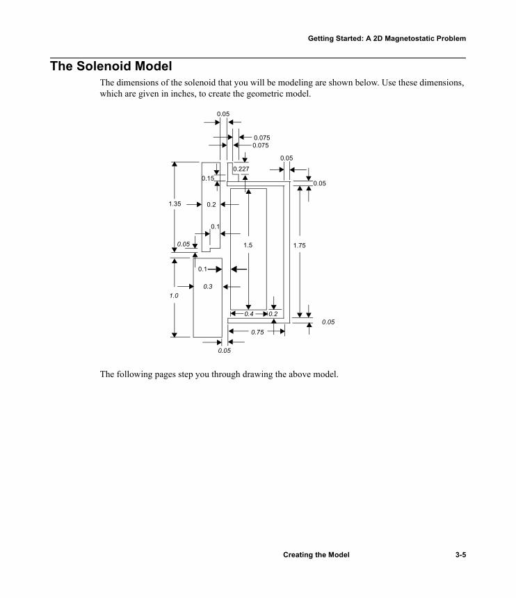
The Solenoid ModelThe dimensions of the solenoid that you will be modeling are shown below. Use these dimensions, which are given in inches, to create the geometric model.
The following pages step you through drawing the above model.
0.05
0.050.75
0.05
0.4
1.5
1.0
1.750.05
0.3
0.05
0.2
0.1
0.150.227
0.0750.075
0.2
0.05
0.1
1.35
Creating the Model 3-5

Getting Started: A 2D Magnetostatic Problem
Set Up the Drawing RegionThe first step in using the 2D Modeler is to specify the drawing units to use in creating the model. In this case, you must change the units from millimeters to inches. To set up the drawing region:1. Click Model>Drawing Units from the menu bar. The Drawing Units window appears.
2. Select Inches.3. Click the Rescale to new units radio button so the drawing area size will be converted to
inches.4. Click OK.The units are changed from millimeters to inches, and inches now appears next to UNITS in the status bar.
Note Throughout the rest of this guide, all commands will be given as Menu>Command. For example, the command you just used to change the drawing units would be given as: Click Model>Drawing Units.
3-6 Creating the Model

Getting Started: A 2D Magnetostatic Problem
Change the Drawing SizeBecause the size of the solenoid model is relatively small compared to the area now represented on the screen, you will need to reduce the size of the drawing space.To change the drawing size:1. Click Model>Drawing Size. The Drawing Size window appears.
2. The Minima fields set the coordinates for the lower-left corner of the drawing. Change the Minima coordinates to (0,–4.5) by doing the following:
a. Leave the Minima R value set to 0.
b. Double-click the left mouse button in the Minima Z field.c. Type -4.5.
3. The Maxima fields set the coordinates for the upper-right corner of the drawing. Change the Maxima coordinates, using the procedure you just used to change the Minima coordinates:
a. Change the Maxima R value to 3.b. Change the Maxima Z value to 4.5.
4. Click OK.
Note Because the simulator assumes that the Z-axis (the left edge of the drawing region) represents the axis of rotational symmetry in an axisymmetric model, you cannot enter a value for R that is less than zero.
Creating the Model 3-7
Getting Started: A 2D Magnetostatic Problem
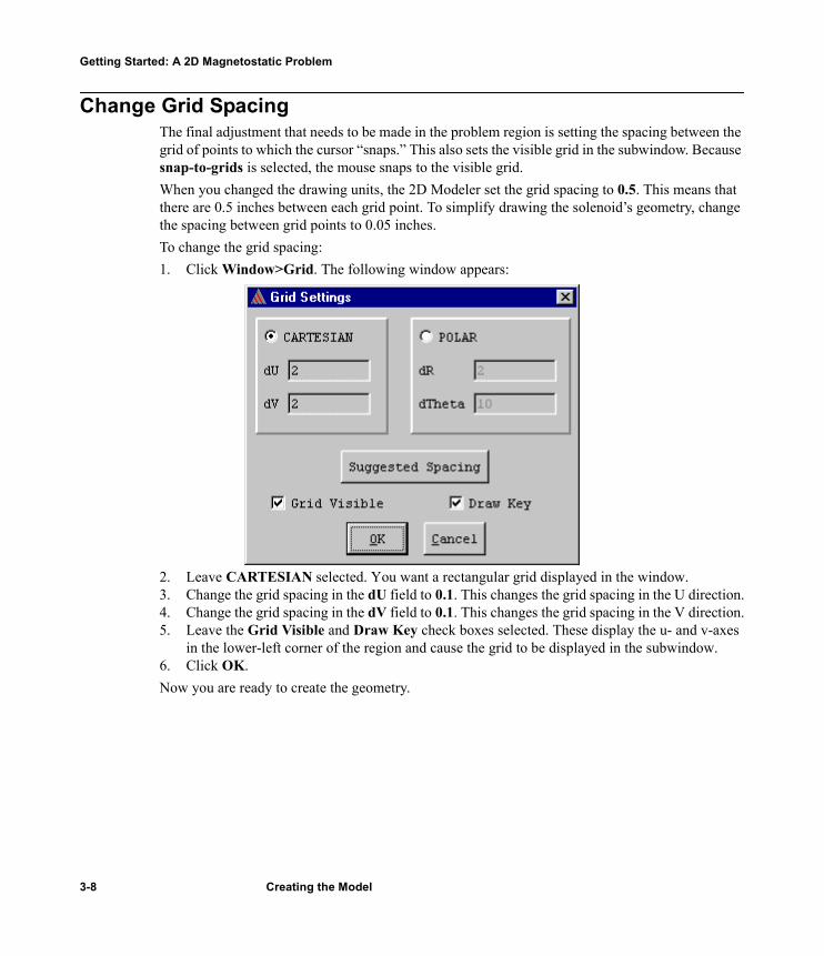
Change Grid SpacingThe final adjustment that needs to be made in the problem region is setting the spacing between the grid of points to which the cursor “snaps.” This also sets the visible grid in the subwindow. Because snap-to-grids is selected, the mouse snaps to the visible grid.When you changed the drawing units, the 2D Modeler set the grid spacing to 0.5. This means that there are 0.5 inches between each grid point. To simplify drawing the solenoid’s geometry, change the spacing between grid points to 0.05 inches.To change the grid spacing:1. Click Window>Grid. The following window appears:
2. Leave CARTESIAN selected. You want a rectangular grid displayed in the window.3. Change the grid spacing in the dU field to 0.1. This changes the grid spacing in the U direction.4. Change the grid spacing in the dV field to 0.1. This changes the grid spacing in the V direction.5. Leave the Grid Visible and Draw Key check boxes selected. These display the u- and v-axes
in the lower-left corner of the region and cause the grid to be displayed in the subwindow.6. Click OK.Now you are ready to create the geometry.
3-8 Creating the Model

Getting Started: A 2D Magnetostatic Problem
Create the GeometryThe solenoid is made up of five objects: a plugnut, core, coil, yoke, and bonnet. All objects are cre-ated using the Object commands as described in the following sections.A sixth object — the “background” object — contains all areas of the model that are not occupied by other objects and does not have to be explicitly drawn. The background object is used when defining material properties and boundary conditions in Chapter 4, “Setting Up the Model.”
Draw the PlugnutFirst, draw the plugnut, and specify its name and color.
Create a RectangleTo create the plugnut:1. Click Object>Rectangle. The cursor turns into crosshairs and the following text appears in the
message bar:MOUSE LEFT: Select first corner point of rectangle�MOUSE RIGHT: Abort command
2. Select the first corner of the plugnut, the upper-left corner, as follows:a. Move the mouse to the point on the grid where the u- and v-coordinates are (0, –0.2). �
Remember that the coordinates of the cursor’s current location are displayed in the U and V fields in the status bar.
b. Click the left mouse button to select the point. A new message appears in the message bar:
MOUSE LEFT: Select second corner point of rectangle�MOUSE RIGHT: Abort command
3. Select the second corner, the lower right corner, as follows:a. Move the mouse to the point on the grid where the u- and v-coordinates are (0.3, –
1.2).b. Click the left mouse button to select the point.
The New Object window appears.
Creating the Model 3-9

Getting Started: A 2D Magnetostatic Problem
Change the Plugnut’s Name and Color By default, the object you are creating is assigned the name object1 and the color red. The field Name is selected by default. To change the name and color:1. Type plugnut in the Name field. 2. Click the left mouse button on the red box. A palette of 16 colors appears.3. Click on the blue box in the palette.4. Click OK.The object now appears as shown below. It is blue and has the name plugnut.
Keyboard EntryIn the “Change the Drawing Size” section, you changed the drawing units from millimeters to inches and left the default grid spacing set to 0.1 inches. However, several of the points that you will select as you draw the objects in the solenoid model lie between grid points. You can select those in-between points in one of two ways:• Use keyboard entry, that is, enter the coordinates directly into the U and V fields in the status
bar.• Change the grid spacing to produce a tighter grid. If you do this, the screen may become clut-
tered with tightly-spaced grid points and make point selection difficult.Use keyboard entry to enter several of the dimensions of the solenoid’s geometry.
Note As you enter points using the keyboard, be careful that you do not move the mouse. If the cursor leaves the status area, the coordinates will change to reflect the cursor’s new position.
3-10 Creating the Model

Getting Started: A 2D Magnetostatic Problem
Draw the CoreUse the Object>Polyline command to draw the irregular solenoid core.To draw the core of the solenoid:1. Click Object>Polyline. The following text appears in the message bar:
MOUSE LEFT: Click to enter point, click at previous point to finish �MOUSE Right: Back up to previous point
2. Click the left mouse button at the u-and v-coordinates (0.1, 1.2) to select the first point of the core.
3. Click the left mouse button at the u-and v-coordinates (0.1, –0.15) to select the next point. A line connects the two points.
4. Select the following points in the same manner:
5. Double-click at (0.1, 1.2) to complete the object, or press Enter twice. The New Object win-dow appears, prompting you to change the object’s name.
6. Change the Name to core, its Color to light green, and click OK.The completed core should appear as shown below:
U V0.2 –0.150.2 –0.10.3 –0.10.3 1.2
Creating the Model 3-11

Getting Started: A 2D Magnetostatic Problem
Draw the CoilTo draw the coil using keyboard entry:1. Click Object>Rectangle.2. To select the first corner of the coil, enter its coordinates on the keyboard. The u-coordinate of
the upper left corner, 0.375, lies between grid points. Select this corner as follows:a. Double-click in the U field in the status bar. b. Type 0.375.c. Press the Tab key to move to the V field in the status bar. d. Type 0.7.e. Do one of the following to accept the point:• Press Return.• Click Enter from the status bar.
3. Select the lower right corner of the coil (0.775, – 0.8) in the same way:a. Enter 0.775 in the U field in the status bar.b. Enter –0.8 in the V field in the status bar.c. Press Return or click Enter from the status bar to accept the point.
The New Object window appears, prompting you to change the object’s color and name.4. Change the object’s Name to coil and its Color to red, and then click OK.The coil should appear as shown below:
Note From this point on, help text that is displayed in the message bar will generally not be included in this manual. Therefore, be sure to look at the message bar if you need to know what effect clicking a mouse button has for a command.
3-12 Creating the Model

Getting Started: A 2D Magnetostatic Problem
Save the Geometry Maxwell SV does not automatically save your work while you are drawing. It is a good idea to periodically save the geometry while you are working on it.To save the solenoid model, click File>Save. The geometry is saved in a file called solenoid.sm2 in the solenoid.pjt directory (in which the files for the solenoid project are stored). This directory is located under the getting_started_SV project directory.
Draw the YokeAfter you draw the coil and save the geometric model, draw the yoke for the solenoid.To draw the solenoid’s yoke:1. Click Object>Polyline, and then click on the point (0.35, –1.05) to select the first corner of the
yoke. Click OK after clicking on the point for the first corner.2. Select the remaining points for the yoke, using the following coordinates:
After you enter the final coordinate (0.35, –1.05), press Enter twice. The New Object window appears.
3. Change the object’s Name to yoke and its Color to purple, and click OK.
U V1.1 –1.051.1 0.80.35 0.80.35 0.751.05 0.751.05 –1.00.35 –1.00.35 –1.05
Creating the Model 3-13

Getting Started: A 2D Magnetostatic Problem
Draw the BonnetThe last object you need to draw is the bonnet. Use keyboard entry to specify coordinates that lie between grid points.To draw the bonnet:1. Click Object>Polyline. 2. To select the first corner of the bonnet, use the keyboard to enter the following coordinates:
3. After selecting the point, press the Tab key to highlight the U field again.4. To select the remaining points, use the keyboard to enter the following coordinates:
After entering the final point in the bonnet (0.35, 0.8) twice, the New Object window appears. 5. Change the object’s Name to bonnet and its Color to light blue, and click OK.
Completed GeometryThe geometric model is now complete.
U 0.35 Press Tab.V 0.8 Press Return.
U V0.50 0.80.50 0.950.425 0.950.425 1.1770.35 1.1770.35 0.80.35 0.8
3-14 Creating the Model

Getting Started: A 2D Magnetostatic Problem
Exit the 2D ModelerTo save your model and exit:1. Click File>Exit. A message appears asking if you want to save the subwindow settings as the
defaults for new ones.2. Click No. You do not need to use the grid settings for the solenoid model as the default for new
projects. A new message appears:Save changes to “solenoid” before closing?
3. Click Yes.The geometry is saved in the solenoid.pjt directory, and the Executive Commands menu reap-pears. A check mark appears next to Define Model, indicating that this step has been completed.
Note The Group Objects command under Define Model is not required for setting up a model in Maxwell SV. For this example, none of the objects you created are connected at any point in a 3D rendering of the model; therefore, you do not need to group any objects. See the Maxwell 2D online help for further details on grouping objects.
Creating the Model 3-15

Getting Started: A 2D Magnetostatic Problem
3-16 Creating the Model

Setting Up the Model
Now that you have drawn the geometry for the solenoid problem and returned to the Executive Commands menu, you are ready to set up the model. The goals for this chapter are to:• Assign materials with the appropriate material attributes to each object in the geometric model.• Define any boundary conditions and sources that need to be specified, such as the source �
current of the coil.• Request that the force acting on the core be calculated during the solution.
Time This chapter should take approximately 30 minutes to work through.
Setting Up the Model 4-1
Getting Started: A 2D Magnetostatic Problem
Assign Materials to Objects The next step in setting up the solenoid model is to assign materials to the objects in the model. Materials are assigned to objects via the Material Manager, which is accessed through the Setup Materials command. You will do the following:• Assign copper to the coil.• Define the material cold rolled steel (a nonlinear magnetic material) and assign it to the bonnet
and yoke.• Define the material Neo35 (a permanent magnet) and assign it to the core.• Define the material SS430 (a nonlinear magnetic material) and assign it to the plugnut.• Accept the default material that is assigned to the background object, which is vacuum.
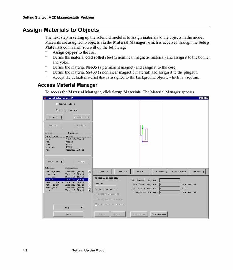
Access Material ManagerTo access the Material Manager, click Setup Materials. The Material Manager appears.
4-2 Setting Up the Model

Getting Started: A 2D Magnetostatic Problem
Assign Copper to the CoilThe Material Manager should still be on the screen. In the actual solenoid, the coil is made of �copper. To assign the material copper to the coil:1. Select the object that is to be assigned a material — the coil — in one of two ways:
• Click the name coil in the Object list.• Click the object coil in the geometry.Both the object and its name are highlighted.
2. Select copper from the Material database listing. If it does not appear in the box, use the scroll bars to pan through the list as described in Chapter 3, “Creating the Model.”
3. Click the Assign button, which is located above the Material list.Copper now appears next to coil in the Objects list.
Assign Cold Rolled Steel to the Bonnet and Yoke The bonnet and yoke of the solenoid are made of cold rolled steel. Since this material is not in the database, you must create a new material, ColdRolledSteel. This material is nonlinear — that is, its relative permeability is not constant and must be defined using a B vs. H curve. Therefore, when you enter the material attributes for cold rolled steel, you will also define a B-H curve.
Select Objects and Create the MaterialTo select the objects and create the new material:1. If it is not already selected, select the Multiple Select radio button from the top of the menu.2. Select bonnet and yoke.3. Click Material>Add from the Material pull-down menu.4. Under Material Properties, change the name of the new material from Material80 to Cold-
RolledSteel.5. Select B-H Nonlinear Material. The Rel. Permeability (Mu) field changes to a button
labeled B H Curve.
Note To deselect an object, simply click on it. To select multiple objects from the Object list, click Multiple Select, and hold down the Ctrl key and click each object.
As an alternative to selecting and deselecting objects with the mouse, use the Select commands (which appear beneath the Multiple Select button in the Material Manager). They are described in Maxwell 2D’s online help.
Setting Up the Model 4-3
Getting Started: A 2D Magnetostatic Problem
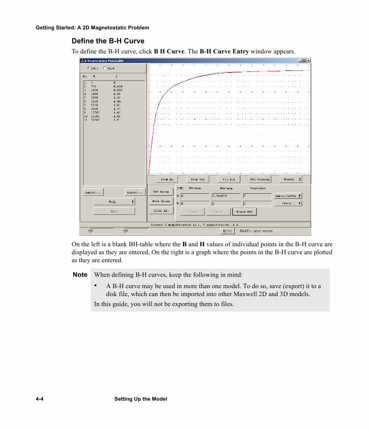
Define the B-H Curve To define the B-H curve, click B H Curve. The B-H Curve Entry window appears.
On the left is a blank BH-table where the B and H values of individual points in the B-H curve are displayed as they are entered. On the right is a graph where the points in the B-H curve are plotted as they are entered.
Note When defining B-H curves, keep the following in mind:
• A B-H curve may be used in more than one model. To do so, save (export) it to a disk file, which can then be imported into other Maxwell 2D and 3D models.
In this guide, you will not be exporting them to files.
4-4 Setting Up the Model

Getting Started: A 2D Magnetostatic Problem
Define the Minimum and Maximum Values for B and HBefore entering the curve’s B and H values, you need to make sure the data will fit on the graph. Minimum and maximum values for the graph are entered under AXES. The H values for cold rolled steel will fall between zero and 35,000 amperes per meter. The B values will fall between zero and 2.0 tesla.To change the graph size:1. Enter 0 in the Minimum H field.2. Enter 0 in the Minimum B field.3. Enter 35000 in the Maximum H field.4. Enter 2 in the Maximum B field.5. Click Accept.
Add B-H Curve Points To enter the points in the B-H curve:1. Click Add Point.2. Click the left mouse button at the point (0, 0) — the origin of the B- and H-axes. The coordi-
nates are displayed in the H and B fields in the status bar. The values for H and B are entered in the B-H Curve table, and a point is entered on the graph.
3. To enter the rest of the values for the B-H curve, do the following:a. To enter the next point, double-click in the H field in the status bar.b. Enter 779. Press the Tab key to go to the B field.c. Enter 0.644.d. Click Enter. Press Tab again to return to the H field.
A line connects the two points on the curve.4. Repeat step three, entering the following data:
Note Numeric values — like the minimum and maximum B and H values — may be entered and displayed in Ansoft’s shorthand for scientific notation. For instance, 35000 could also be entered as 3.5e4. When entering numeric values, you can use either notation.
H B 1080 0.858
1480 1.06
2090 1.26
3120 1.44
5160 1.61
9930 1.77
1.55e4 1.86
Setting Up the Model 4-5
Getting Started: A 2D Magnetostatic Problem
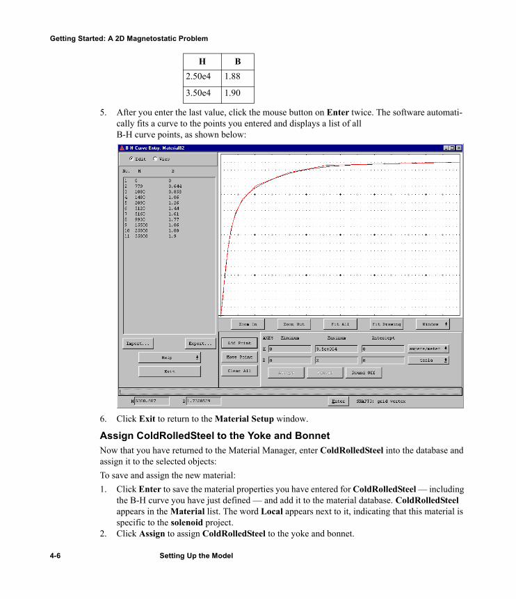
5. After you enter the last value, click the mouse button on Enter twice. The software automati-cally fits a curve to the points you entered and displays a list of all �B-H curve points, as shown below:
6. Click Exit to return to the Material Setup window.
Assign ColdRolledSteel to the Yoke and BonnetNow that you have returned to the Material Manager, enter ColdRolledSteel into the database and assign it to the selected objects:To save and assign the new material:1. Click Enter to save the material properties you have entered for ColdRolledSteel — including
the B-H curve you have just defined — and add it to the material database. ColdRolledSteel appears in the Material list. The word Local appears next to it, indicating that this material is specific to the solenoid project.
2. Click Assign to assign ColdRolledSteel to the yoke and bonnet.
2.50e4 1.88
3.50e4 1.90
H B
4-6 Setting Up the Model

Getting Started: A 2D Magnetostatic Problem
Assign Neo35 to the CoreNext, create the new material Neo35, and assign it to the core. Neo35 is a permanently magnetic material.
Select the Object and Create the MaterialTo select the core and create the material:1. Select core from the Object list. 2. Click Material>Add.3. Under Material Properties, change the name of the new material to Neo35.
Select Independent Material PropertiesIn magnetostatic problems, only two of the four available material properties need to be specified. The values of the other two properties are dependent upon these properties, according to the rela-tionships shown below.
You will be specifying values for relative permeability, �, and magnetic retentivity, Br. The values of the other two properties, magnetic coercivity, Hc, and magnetization, Mp, will be computed using the relationships shown above.
Note In the actual solenoid, the core was assigned the same material as the plugnut — SS430. However, for this problem, a permanent magnet is assigned to the core to demonstrate how to set up a permanent magnetic material.
B
HHc
MagneticCoercivity
BrMagnetic
Retentivity Br �oMp �o�rHc= =
� = Br/Hc
Setting Up the Model 4-7

Getting Started: A 2D Magnetostatic Problem
To specify which properties are to be entered:1. Click Options. The Property Options window appears.
Initially, the only properties that can be specified are the relative permeability (�r) and the magnetic coercivity (Hc). To define the permanent magnet, you will need to specify the magnetic retentivity.2. Click on the check box next to Hc to deselect it.3. Click on the check box next to Br to select it.4. Click OK.
Enter Material PropertiesNow enter the values for the material attributes of Neo35. Only the two material attributes that were turned on in the Property Options window need to be entered — the other two attributes will be calculated automatically.To enter the properties for Neo35:1. Enter 1.05 in the Rel. Permeability (Mu) field.2. Enter 1.25 in the Mag. Retentivity (Br) field. Values automatically appear in the other fields.3. Click Enter.Neo35 is now listed as a local material in the database.
4-8 Setting Up the Model

Getting Started: A 2D Magnetostatic Problem
Assign Neo35 to the Core and Specify Direction of MagnetizationNow that you have created the material Neo35, all that remains is to assign it to the core and spec-ify the direction of magnetization. By default, the direction of magnetization in materials is along the R-axis (or the x-axis). However, in this problem, the direction of magnetization in the core points along the positive z-axis. To model this, you must change the direction of magnetization to act at a 90� angle from the default.To assign Neo35 to the core:1. Make certain that Neo35 is highlighted in the Material list.2. Click Assign to assign the material Neo35 to the core object. The Assign Coordinate System
window appears.
3. Select Align with a given direction to align the magnetization with the entered value. 4. Enter 90 degrees in the Angle field.
5. Click OK.
Note Make certain you enter a positive value for the angle. For instance, if you had entered 90 degrees, the magnetization of the core would point in the opposite direction and would tend to push the core out of the solenoid.
Setting Up the Model 4-9

Getting Started: A 2D Magnetostatic Problem
Assign SS430 to the Plugnut Next, create a new material — SS430 — for the plugnut. Like the material ColdRolledSteel, it is a nonlinear material whose relative permeability must be defined using a B-H curve. The first step includes selecting the plugnut and creating the material.
Select Objects and Create MaterialTo select the plugnut, and create the material:1. Select plugnut from the Object list. 2. Click Material>Add.3. Under Material Properties, change the name of the new material to SS430.4. Select B-H Nonlinear Material.
Define the B-H Curve To define the B-H curve for SS430, click B H curve.The B-H Curve Entry window appears.
Define Maximum and Minimum Values for B and HFor SS340, the values for H will fall between zero and 40,000 amperes per meter. The values for B will fall between zero and 2.0 tesla. To change the graph size of the B-H curve:1. Enter 0 in the Minimum H field.2. Enter 0 in the Minimum B field.3. Enter 40000 in the Maximum H field.4. Enter 2.0 in the Maximum B field.5. Click Accept.
Add B-H Curve PointsTo enter the points in the B-H curve:1. Click Add Point.2. Click the left mouse button at the origin of the B- and H-axes (0, 0).3. Enter the following points using keyboard entry, as described under “Define the B-H Curve” in
“Assign Cold Rolled Steel to the Bonnet and Yoke.”H B
143 0.125 180 0.206 219 0.394 259 0.589 298 0.743 338 0.853 378 0.932
4-10 Setting Up the Model

Getting Started: A 2D Magnetostatic Problem
4. After you enter the last value, click Enter twice. The software automatically fits a curve to the points you entered on the graph, as shown below:
5. Click Exit to return to the Material Setup window.
438 1.01 517 1.08 597 1.11 716 1.16 955 1.20 1590 1.27 3980 1.37 6370 1.431.19e4 1.492.39e4 1.553.98e4 1.59
H B
Setting Up the Model 4-11

Getting Started: A 2D Magnetostatic Problem
Assign SS430 to the PlugnutFinally, add SS430 to the material database, and assign it to the selected object:To add and assign SS430:1. Click Enter to save the material attributes you entered for SS430 and add it to the material
database.2. Make certain SS430 is selected in the Material list.3. Click Assign to assign SS430 to the plugnut.
Accept Default Material for BackgroundAccept the following default parameters for the object background:• The material vacuum, which has the material attributes of a vacuum. The object background
is the only object that is assigned a material by default.• Include it as part of the problem region in which to generate the solution. When a material
name — such as vacuum, the material that is assigned to background by default — appears next to background in the Object list, it is included as part of the solution region.
Exit the Material ManagerNow that materials have been assigned to each object, exit the Material Setup window:To exit the Material Setup window:1. Click Exit from the bottom-left of the Material Setup window. A window with the following
prompt appears:Save changes before closing?
2. Click Yes.You are returned to the Executive Commands menu. A check mark now appears next to Setup Materials, and Setup Boundaries/Sources remains enabled.If you exit the Material Manager before assigning a material to each object in the model, a check mark does not appear next to Setup Materials on the Executive Commands menu, and Setup Boundaries/Sources is disabled. You will not be allowed to continue setting up your model until materials are assigned to all objects in the model.
Set Up Boundaries and Current SourcesAfter you set material properties, you must define boundary conditions and sources of current for the solenoid model. Boundary conditions and sources are defined in the Boundary Manager, which is accessed through the Setup Boundaries/Sources command.By default, the surfaces of all objects are Neumann or natural boundaries. That is, the magnetic field is defined to be perpendicular to the edges of the problem space and continuous across all object interfaces. To finish setting up the solenoid problem, you must explicitly define the follow-ing boundaries and sources:• The boundary condition at all surfaces exposed to the area outside of the problem region.
Because you included the background as part of the problem region as described in the “Accept Default Material for Background” section, this exposed surface is that of the object
4-12 Setting Up the Model

Getting Started: A 2D Magnetostatic Problem
background. Since the solenoid is assumed to be very far away from other magnetic fields or sources of current, those boundaries will be defined as “balloon boundaries.”
• The source current on the coil. Since the coil has 10,000 turns of wire, and one ampere flows through each turn, the net source current is 10,000 amperes.
Access the 2D Boundary/Source ManagerDefine the boundary conditions for the model. To access the Boundary Manager:• Click Setup Boundaries/Sources. The 2D Boundary/Source Manager appears.
Boundary Manager Screen LayoutMenu Bar and ToolbarLike 2D Modeler commands, 2D Boundary/Source Manager commands may be accessed from the following:• The menu bar, which is located along the top of the 2D Boundary/Source Manager window. • The toolbar, which is located on the top of the window.
Note Maxwell SV will not solve the problem unless you specify some type of source or magnetic field — either a current source, an external field source using boundary conditions, or a permanent magnet. In this problem, both the permanent magnet assigned to the core and the current flowing in the coil act as magnetic field sources.
Setting Up the Model 4-13

Getting Started: A 2D Magnetostatic Problem
BoundaryEach time you choose one of the Assign>Boundary or Assign>Source commands, an entry is added to the Boundary list on the left side of the menu. When you first access the 2D Boundary/Source Manager, the Boundary list is empty.Display AreaThe geometric model is displayed on the menu so that you can choose objects using the Edit>Select commands. Use the Window>Change View commands, described in the Maxwell 2D online help, to change your view of the model.Boundary/Source InformationThe box that appears below the geometric model allows you to assign boundaries and sources to objects and surfaces, and to display the parameters associated with the selected boundary or source.
Types of Boundary Conditions and SourcesThere are two types of boundary conditions and sources that you will use in this problem:
In this example, you will assign boundary conditions and sources to the following objects in the solenoid geometry:
Set Source Current on the CoilBefore you identify a boundary condition or source, you must first identify the object or surface to which the condition is to be applied. In this section, you will pick the coil as a source and then assign a current to it.Pick the CoilTo select the coil as a source:1. Click Edit>Select>Object>By Clicking.2. Click the left mouse button on the object coil, highlighting it.3. Click the right mouse button anywhere in the display area to stop selecting objects.
Balloon �boundary
Can only be applied to the outer boundary. Models the case in which the structure is infinitely far away from all other electromagnetic sources.
Solid source Specifies the DC source current flowing through an object in the model.
Background At the outer boundary of the problem region, the outside edges of this surface are to be ballooned to simulate an insulated system.
Coil This object is to be defined as a 10,000-amp DC current source. The current is uniformly distributed over the cross-section of the coil and flows in the positive perpendicular direction to the cross-section.
Note If the appropriate object is not highlighted, or if more than one object is highlighted, do the following:1. Click Edit>Deselect All. After you do, no objects are highlighted.2. Follow the instructions again to pick the object.
4-14 Setting Up the Model

Getting Started: A 2D Magnetostatic Problem
Assign a Current Source to the CoilTo specify the current flowing through the coil:1. Click Assign>Source>Solid. The name source1 appears in the Boundary list, and NEW
appears next to source1, indicating that the source has not yet been assigned to an object or surface. Fields appear in the boundary information area at the bottom of the window:
2. Leave the Current check box selected.3. Leave the Total radio button selected.4. Enter 10000 in the Value field, and click Assign. The label current replaces NEW next to
source1 in the Boundary list.
Assign Balloon Boundary to the BackgroundThe structure is a magnetically isolated system. Therefore, you must create a balloon boundary by assigning balloon boundaries to the outside edges of the background object.
Pick the BackgroundTo select the background as a boundary.1. Click Edit>Select>Object>By Clicking, and click the left mouse button anywhere on the
background.2. Click the right mouse button to abort the command.Now you are ready to balloon the background.
Assign Balloon BoundaryTo assign a balloon boundary to the background:1. Click Assign>Boundary>Balloon. The balloon1 boundary name appears in the Name field.2. Click Assign. The background is ballooned and balloon replaces NEW next to the boundary
name in the Boundary list.
Note In cartesian (XY) models, all outer edges may be defined as boundaries. However, in axisymmetric (RZ) models, the left edge of the problem region cannot be assigned a boundary condition. Because the solenoid model is axisymmetric (representing the cross-section of a device that is revolved 360 degrees around its central axis), the simulator ignores the balloon boundary you defined on the left edge of the geometry. Instead, it automatically imposes a different boundary condition, in order to model that left edge as an axis of rotational symmetry.
Setting Up the Model 4-15

Getting Started: A 2D Magnetostatic Problem
Exit the Boundary ManagerTo exit the Boundary Manager: 1. Click File>Exit. A window appears with the following message:
Save changes to “solenoid” before closing?2. Click Yes.You return to the Executive Commands menu. A check mark appears next to Setup Boundaries/Sources, indicating that this step has been completed. Note that a check mark also appears next to Setup Solution Options, indicating that a set of default solution parameters has been defined for the problem.You are now ready to set up the force computation for the model.
Set Up Force Computation One of your goals for this problem is to determine the force acting on the core of the solenoid. To find the force on this object, you must select it using the Force command under Setup Executive Parameters. The force (in newtons) acting on the core will then be computed during the solution process.To select the core object for the force computation:1. Click Setup Executive Parameters. The following menu appears:
Force�Core Loss�Torque�Flux Lines�Post Processor Macros�Matrix/Flux�Select Matrix/Flux Entries
Quantities that may not be computed are grayed out and cannot be accessed. The Select Matrix/Flux Entries option is not enabled for Maxwell SV because the student version does not use the parametric analysis capability.
2. Click Force. The Force Setup window appears. All objects in the model are listed on the left
4-16 Setting Up the Model

Getting Started: A 2D Magnetostatic Problem
side of the window. The geometric model is shown on the right.
3. Select the object on which force is to be computed — the core — in one of two ways:• Select core from the Object list.• Click on the object core in the geometry.Both the object and its name are highlighted.
4. To include the core object in the force computation, click Yes next to Include selected objects. The word Yes appears next to core in the Object list.
5. Click Exit to exit the Force Setup window. The following message appears:Save changes before closing?
6. Click Yes to save the force setup and exit. You return to the Executive Commands menu. The force on the core will now be computed during the solution. You are now ready to enter the solution criteria.
Setting Up the Model 4-17

Getting Started: A 2D Magnetostatic Problem
4-18 Setting Up the Model

Generating a Solution
Now you are ready to specify solution parameters and generate a solution for the solenoid model. You will do the following:The goals for this chapter are to:• View the criteria that affect how Maxwell SV computes the solution.• Generate the magnetostatic solution. The axisymmetric magnetostatic solver calculates the
magnetic vector potential, A�, at all points in the problem region. From this, the magnetic field, H, and magnetic flux density, B, can be determined.
• Compute the force on the core. Since you requested force using the Setup Executive Parame-ters command, this automatically occurs during the general solution process.
• View information about how the solution converged and what computing resources were used.
Time This chapter should take approximately 40 minutes to work through.
Generating a Solution 5-1

Getting Started: A 2D Magnetostatic Problem
View Solution CriteriaUse the default criteria to generate the solution for the solenoid problem.To view the solution criteria, click Setup Solution Options. The Solve Setup window appears.
When the system generates a solution, it explicitly calculates the field values at each node in the finite element mesh and interpolates the values at all other points in the problem region.
Starting MeshLeave the Starting Mesh command set to Initial. This instructs the system to use the only mesh available, the coarse initial mesh when it begins the solution process. If you had already generated a solution and wanted to take advantage of the most recently refined mesh, you would click Cur-rent.
Manual MeshTo get a head start on refining the initial mesh or the current mesh, you could choose the Manual Mesh command. This would allow you to manually break large triangles down into smaller ones, increasing the accuracy of the solution in the desired areas.
5-2 Generating a Solution

Getting Started: A 2D Magnetostatic Problem
Solver ChoiceYou can specify which type of matrix solver to use to solve the problem. In the default Auto posi-tion, the software makes the choice. The ICCG solver is faster for large matrices, but occasionally fails to converge (usually on magnetic problems with high permeabilities and small air-gaps). The Direct solver will always converge, but is much slower for large matrices. In the Auto position, the software evaluates the matrix before attempting to solve; if it appears to be ill-conditioned, the Direct solver is used, otherwise the ICCG solver is used. If the ICCG solver fails to converge while the solver choice is in the Auto position, the software will fall back to the Direct solver auto-matically. Leave the Solver Choice option set to Auto.
Solver ResidualLeave the Residual field set to 0.001 for Linear, and to 0.005 for Nonlinear. These values specify how close each solution must come to satisfying the equations that are used to compute the mag-netic field.
Solve for Fields and ParametersThe Solve for options tell the system what types of solutions to generate.
Leave both the Fields and Parameters check boxes selected, to solve for both fields and parame-ters in this example.
Adaptive AnalysisDo the following to have the system adaptively refine the mesh and solution:• Leave Adaptive Analysis selected. Doing so instructs the system to solve the problem itera-
tively, refining the regions of the mesh in which the largest error exists. Refining the mesh makes it more dense in the areas of highest error, resulting in a more accurate field solution.
• Leave Number of requested passes and Percent error set to their defaults. After each itera-tion, the system calculates the total energy of the system and the percentage of this energy that is caused by solution error. It then checks to see if the number of requested passes has been completed, or if the percent error and the change in percent error between the last two passes match the requested values.
• Leave Percent refinement per pass set to its default value. In most cases, the default refine-ment value is acceptable.
If any of these criteria has been met, the solution process is complete and no more iterations are done.
Exit Setup Solution OptionsTo exit the Solve Setup window, click OK. You return to the Executive Commands menu.
Fields A field solution is generated.
Parameters Any quantities that you set up using the Setup Executive Parameters command are computed (in this case, the force on the core).
Generating a Solution 5-3
Getting Started: A 2D Magnetostatic Problem
Start the Solution Now that you have examined the solution parameters, the problem is ready to be solved. To start the solution, click Solve.The solution process begins and the following changes occur:• The system creates the initial finite element mesh for the solenoid structure. A bar labeled
Making Initial Mesh appears in the Solution Monitoring area at the bottom of the screen. It shows the system’s progress as it generates the mesh.
• A bar labeled Solving Fields appears in the Solution Monitoring area.• A button labeled Abort appears next to the progress bar and remains there throughout the
entire solution process. If desired, you can use it to stop the solution process.• A bar labeled Setting up solution files appears.After the system makes the initial finite element mesh, the magnetostatic field solution process begins. Values you obtain for percent energy error, total energy, or force may differ slightly from the ones given in this guide. Depending upon how closely you followed the directions for setting up the solenoid model, the results that you obtain should be approximately the same as the ones given here.
Monitoring the SolutionThe following monitoring bars alternate in the Solution Monitoring box at the bottom of the menu. They allow you to monitor the system’s progress as it computes each adaptive pass (solve — error analysis — refine cycle) of the magnetostatic solution. Periodically, the solver also displays messages beneath the progress bars. The following table explains some of the messages that may appear:
Solving Fields Displayed as Maxwell SV computes the field solution. After it finishes computing a solution, it identifies the triangles that have the highest energy error.
Refining �Mesh
Displayed as the system refines the regions of the finite element mesh with the highest error energy. Since the default specification for mesh refinement is 15 percent, the system refines triangles that have the top 15 percent of the error.
Solving matrix �(nonlinear itera-tion)
Displayed as the system calculates a solution for the relationship between the current and the field solution. This may go on for several iterations before the general field solution continues. Because there are nonlinear materials in the model, the magnetostatic field solver uses a somewhat different solution process than if linear materials were present.
Computing force value
Displayed as the simulator solves for the force on the core due to the source current in the coil.
5-4 Generating a Solution

Getting Started: A 2D Magnetostatic Problem
Viewing Convergence DataAfter a few adaptive passes are completed, click the Convergence button at the top of the Execu-tive Commands menu to monitor how the solution is progressing. Convergence information appears as shown below. In this example, the system has completed eight adaptive passes.
Solution CriteriaInformation about the solution criteria is displayed on the left side of the convergence display.
Number of passes Displays how many adaptive passes have been completed and still remain.
Target�Error
Displays the percent error value — 1% — that was entered using the Setup Solution Options command.
Energy �Error
Displays the percent error from the last completed solution — in this case, 0.754%. Allows you to see at a glance whether the solution is close to the desired error energy.
Delta �Energy
Displays the change in the total energy between the last two solutions — in this case, 0.144%. Because this value and the Energy Error value are less than the Target Error, the solution is considered to be converged.
Generating a Solution 5-5
Getting Started: A 2D Magnetostatic Problem
Completed SolutionsInformation about each completed solution is displayed on the right side of the screen.
Completing the Solution ProcessWhen the solution is complete, a pop-up window with the following message appears:
Solution Process is complete
Click OK to continue.You are now ready to view final convergence information for the completed solution.
Pass Displays the number of the completed solutions. In the previous figure, eight adaptive passes were completed.
Triangles Displays the number of triangles in the mesh for a solution. In the previous figure, the mesh used for the eighth solution had 826 triangles.
Total Energy (J) Displays the total energy of a solution in Joules. In the previous figure, the total energy for the eighth solution was 1.98714 Joules.
Energy Error (%) Displays the percent energy error of the completed solutions. In the previous figure, the energy error for the eighth solution was .7543%.
Mag Force �(N)
Displays the magnitude of the force on the core in newtons. Force is computed after each adaptive pass, allowing you to see if it is converging to a stable value. In the previous figure, the force on the core during the tenth solution was 1.17639E+02, or 117.459 newtons. This value only represents the total force acting on the object and does not indicate its direction.
Note After a solution is generated, the system does not allow you to change the geometry, material properties, or boundary conditions of the model unless you first delete the solution. Therefore, you must generate a new solution if you change the model.
5-6 Generating a Solution

Getting Started: A 2D Magnetostatic Problem
Viewing Final Convergence DataIf convergence data is not displayed on the screen, click Convergence again.
Note If a problem does not begin to converge after several adaptive passes, the problem is probably ill-defined — for instance, boundary conditions may not have been specified correctly. If this ever happens, do the following to interrupt the solution process:
1. Click the Abort button in the Solution Monitoring box. 2. Check the problem definition, and then solve the problem again.
Generating a Solution 5-7

Getting Started: A 2D Magnetostatic Problem
Plotting Convergence DataBy default, convergence data is displayed in table format as shown in the previous figure. This data can also be displayed graphically. To plot the magnitude of force computed during each adaptive pass:• Click Convergence Display>Plot Force from the bottom of the display area. The following
plot appears:
Displaying this data graphically often makes it easier to see how the solution is converging. For instance, above, the curve begins to level off after the second pass as the total force starts to stabi-lize.Optionally, use the other commands under Convergence Display to plot the number of triangles, total energy, or percent error for all adaptive passes.
5-8 Generating a Solution

Getting Started: A 2D Magnetostatic Problem
Viewing Statistics Click Profile from the top of the Executive Commands menu to see what computing resources were used during the solution process. The following screen appears.
The time that the solution process began is displayed at the top of the box. Beneath it, the following information is displayed for each adaptive field solution and mesh refinement step that was com-pleted:
If more data is available than can fit on a single screen, scroll bars appear. To display more data, manipulate the display as described in Chapter 3, “Creating the Model”
Command/Info
Displays the name of the system command that was used.
Real time Displays the time taken to complete the step.Cpu time Displays the amount of time taken by the CPU (central
processing unit) to complete the step.Mem size Displays the amount of memory used.Num ElementsDisplays the of number of triangles in the finite element mesh.
Generating a Solution 5-9

Getting Started: A 2D Magnetostatic Problem
5-10 Generating a Solution

Analyzing the Solution
Now that you have generated a magnetostatic solution for the solenoid problem, you can analyze it using Maxwell SV’s post processing features.The goals for this chapter are to:• Examine computed force values.• Plot the magnetic flux and magnetic fields in and around the solenoid.• Observe the nonlinear properties of the model using B-H curves.
Time This chapter should take approximately 25 minutes to work through.
Analyzing the Solution 6-1

Getting Started: A 2D Magnetostatic Problem
View Force SolutionNow that the solution is complete, examine the results of the force computation. To view the force results, click Solutions>Force. The final force value computed during the adap-tive solution appears as shown below.
• The object(s) that were selected for the force computation — in this case, the core — are listed under Force Setup Objects.
• The results of the force solution (each force component) are given under Force Value (new-tons). The net force on the core is approximately 117.459 newtons, acting in the negative z direction (pulling the core down into the solenoid). There is no component of force in the r direction because of the axial symmetry.
Access the Post ProcessorUse the 2D Post Processor to plot the lines of magnetic flux and saturation levels in materials. To access the Post Processor, click Post Process. The 2D Post Processor appears.
6-2 Analyzing the Solution

Getting Started: A 2D Magnetostatic Problem
Post Processor Screen LayoutThis section provides a brief overview of the 2D Post Processor. For further details, refer to the Post Process section in the Maxwell 2D online help.
General Areas The Post Processor is divided into the following general areas:.
Plot the Magnetic FieldAll objects created in the modeler, plus the background, represent the modeling region.
Menu Bar The menu bar appears at the top of the Post Processor window.Viewing WindowThe model appears in what is called the viewing window. This window
displays the project name, solenoid, in its title bar.Side Window This area displays the vertex and snap behavior, and lists the coordinates of
the selected points. Status Bar This area displays the following information:
• The version number of Maxwell SV.• The function of each mouse button.
In this project, the balloon boundary is used to model the case where the modeling structure is infinitely far away from other magnetic fields or current sources. Therefore, an object called “balloon” is shown in the On Geometry list in the Create New Plot window (accessed using the Plot>Field command).
To define the problem region for post-processing purposes:1. Click Geometry>Create>Object List. The
object list information appears in the bottom half of the side window.
2. Change the Name to model.3. In the Objects list, select all objects except
balloon, and then click OK.
Analyzing the Solution 6-3
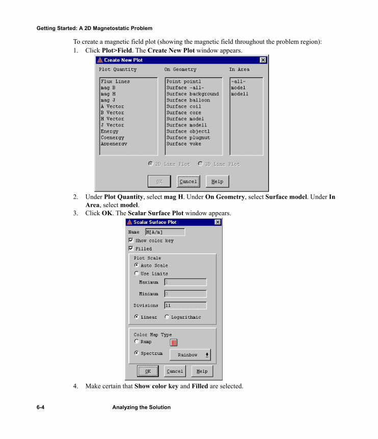
Getting Started: A 2D Magnetostatic Problem
To create a magnetic field plot (showing the magnetic field throughout the problem region):1. Click Plot>Field. The Create New Plot window appears.
2. Under Plot Quantity, select mag H. Under On Geometry, select Surface model. Under In Area, select model.
3. Click OK. The Scalar Surface Plot window appears.
4. Make certain that Show color key and Filled are selected.
6-4 Analyzing the Solution

Getting Started: A 2D Magnetostatic Problem
5. Click OK. The field plot appears. The plot should resemble the following:
Redisplay the Magnetic FIeld PlotNow, redisplay the plot to show a more definitive range of current density distribution. To do this, first zoom in on the model, then redefine the range of values that are displayed. To redisplay the plot:1. Click View>Zoom In. The cursor changes to crosshairs.2. Click the left mouse button on a point to the upper left of the solenoid model.3. Click the left mouse button on a point just to the lower right of the solenoid model. A more
detailed image of the plot appears, allowing you to more easily observe the differences in cur-rent density.
4. Double-click on the plot key. The Scalar Surface Plot window appears.5. Under Plot Scale, select Use Limits.6. Leave the default value in the Maximum field. 7. Enter 10000 in the Minimum field.8. Enter 21 in the Divisions field to display more layers.
Analyzing the Solution 6-5

Getting Started: A 2D Magnetostatic Problem
9. Click OK. The plot should resemble the following one:
Identify Saturated Materials As the final step in your analysis of the solenoid model, you will determine saturation levels in the solenoid’s plugnut. In magnetically saturated materials, large changes in the magnetic field, H, pro-duce relatively small changes in the magnetic flux density, B. In this problem, only the yoke, plug-nut, and bonnet were assigned nonlinear materials. For this example, you will plot the saturation levels in the plugnut.To analyze the saturation level in the plugnut, you will plot the magnetic flux density in the sole-noid to see which areas have a high B-field, and may be saturated. You will then select the object with the highest saturation and plot its B-H curve using the Plot>BH Curves command.
Plot Magnetic Flux DensityThe problem region should still be enlarged as a result of the zoom function in the last step. Now you are ready to plot the magnetic flux density. To plot the magnetic flux density:1. Click Plot>Visibility. The Plot Visibility window appears.2. Select H[A/m] from the list, and click OK. The magnetic field plot is hidden. 3. Click Plot>Field. The Create New Plot window appears. 4. Under Plot Quantity, select mag B. Under On Geometry, select Surface model. Under In
6-6 Analyzing the Solution

Getting Started: A 2D Magnetostatic Problem
Area, select model.5. Click OK. The Scalar Surface Plot window appears.6. Under Plot Scale, select Auto Scale, and click OK. The flux plot appears, showing the mag-
netic flux density of each object in the geometry.Any areas colored completely green, like the one on the upper-right edge of the plugnut, may be saturated.
Analyzing the Solution 6-7

Getting Started: A 2D Magnetostatic Problem
Plot the B-H CurveNow you can plot H versus B, using the Plot>BH Curves command, and graphically view the non-linear properties of the plugnut.To analyze the B-H curve of the plugnut:1. Click Plot>BH Curves. The Select Object B-H Curves window appears. 2. Select plugnut from the list, and click OK. The B-H curve associated with the plugnut
appears, as shown below:
When the B-field in a nonlinear material rises above the “knee” of the material’s B-H curve, further increases in H result in relatively small increases in B. At this point, the material is said to be mag-netically saturated.
6-8 Analyzing the Solution

Getting Started: A 2D Magnetostatic Problem
Exit the Post ProcessorTo exit the 2D Post Processor:1. Click File>Exit from the post processor. A window with the following prompt appears:
Exit Post Processor?2. Click Yes. The Executive Commands window appears.
Exit Maxwell SVOnce you have finished the post processing functions, you are ready to exit the software.To exit Maxwell SV:1. Click Exit from the bottom of the Executive Commands menu. The following prompt
appears: Exit Maxwell SV?
2. Click Yes. The Executive Commands window closes, and the Project Manager reappears.
Exit the Maxwell SoftwareTo exit the Project Manager, click Exit. The Project Manager closes, and the Control Panel reap-pears.To exit the Maxwell Control Panel:1. Click EXIT. A window with the following prompt appears:
Exit Maxwell?2. Click Yes. You return to Microsoft Windows.You have completed Getting Started: A 2D Magnetostatic Problem, the second Getting Started guide for Maxwell SV. (The first guide in the SV Getting Started series is called Getting Started: A 2D Electrostatic Problem.)
Analyzing the Solution 6-9

Getting Started: A 2D Magnetostatic Problem
6-10 Analyzing the Solution

Index
Aadaptive analysis 5-3Ansoft software, installing 1-ivAssign/Boundary commands, Balloon 4-15Assign/Source commands, Solid 4-15axisymmetric models 1-2, 3-2
boundary conditions 4-16drawing size 3-7
Bbackground
and boundary conditions 4-12ballooning 4-15default material for 4-12definition of 3-9extending 4-15including in solution region 4-12
balloon boundaryassigning 4-15definition of 4-14
B-H curveadding points to 4-5, 4-10defining 4-4, 4-10fitting curve to points 4-6for cold rolled steel 4-4
for SS430 4-10keyboard entry 4-5maximum B and H values 4-5, 4-10minimum B and H values 4-5, 4-10plotting saturation levels on 6-8
B-H Plot (Post Processor Plot menu commands) 6-8bonnet
assigning a material to 4-3creating 3-14
boundary conditions 4-12and axisymmetric models 4-16and cartesian models 4-16balloon 4-14, 4-15displaying 4-14for sample problem 4-14screen layout 4-14use of 4-12
buttonsdisabled 2-5
Ccartesian models 3-2coil
assigning a material to 4-3assigning source current to 4-14, 4-15creating 3-12picking as a current source 4-14
Index-1

Getting Started: A 2D Magnetostatic Problem
cold rolled steeldefining as a material 4-3entering B-H curve for 4-4
colors, changing for objects 3-10commands
accessing from menus 3-3, 4-13accessing with the keyboard 3-3accessing with the mouse 3-3accessing with the toolbar 4-13
computing resourcesclock time 5-9commands executed 5-9CPU time 5-9memory size 5-9number of elements 5-9viewing 5-9
Control Panelicon 2-2
Convergence 5-5, 5-7convergence data
delta energy 5-5energy error 5-5, 5-6force 5-6mesh size 5-6number of passes 5-6pass number 5-6plotting 5-8target error 5-5total energy 5-6viewing 5-5, 5-7, 5-8
Convergence Display, Plot Force 5-8coordinate system, uv (local) 3-4coordinates
entering via keyboard 3-4of cursor 3-4
coreassigning a material to 4-10convergence of force solution 5-6, 5-8creating 3-11selecting for force computation 4-17
current 4-14and balloon boundaries 4-15assigning to coil 4-14, 4-15
DDefine Model 1-3, 3-3
Draw Model 1-3Group Objects 1-3
dimensions of sample problem 3-5direct solver 5-3directories, project
creating 2-3selecting 2-4
Draw Model 1-3Drawing 1-3, 3-2drawing plane 3-2drawing region
adjusting view of 2-7, 3-14and axisymmetric models 3-7maximum x- and y-coordinates 3-7minimum x- and y-coordinates 3-7setting up 3-6size of 3-7
Drawing Size 3-7Drawing, RZ Plane 3-2
Eenergy
error 5-3, 5-5, 5-6fluctuations in energy error 5-7total 5-6
errorenergy 5-5, 5-6fluctuations in energy error 5-7of solution 5-3
Executive Commands menu 2-7Convergence 5-5, 5-7Define Model 3-3Drawing 3-2Post Process 6-2Profile 5-9Setup Boundaries/Sources 4-12Setup Executive Parameters 4-16Setup Materials 4-2Setup Solution Parameters 5-1, 5-2
Index-2

Getting Started: A 2D Magnetostatic Problem
Solutions 6-2Solve 5-4Solver 3-2
Exit 3-15, 4-16
Ffield of view
fitting all objects in 2-7, 3-14fitting drawing space in 2-7zooming in on 2-7zooming out of 2-7
fieldsentering text and numbers in 3-7selecting with the mouse 3-7
File commandsExit 3-15, 4-16Open 3-4Save 3-13
files, saving geometry to 3-13Fill Solids 2-7Fit All 2-7Fit Drawing 2-7force
and solution process 4-16components of 6-2computing for the solenoid core 4-16convergence of solution 5-8direction of 6-2magnetic 5-6magnitude of 5-6, 6-2objects in computation 4-17plotting magnitude of 5-8viewing solution results 6-2
Ggeometric models
axisymmetric 1-2, 3-2cartesian 3-2general strategy for creating 3-3saving 3-13
gridchanging point spacing 3-10
in subwindows 3-4modify spacing of 3-8snapping to 3-4
grid points, snapping to 3-4Group Objects 1-3
IICCG solver 5-3installing Ansoft software 1-ivinsulated system 4-15
Kkeyboard
accessing commands with 3-3selecting points with 3-4, 3-10, 3-14, 4-5, 4-10
Mmagnetic coercivity 4-7magnetic field
and balloon boundaries 4-15and saturation 6-6solving for 5-4
magnetic flux densityand saturation 6-6plotting 6-6
magnetic retentivity 4-7magnetization
relationship to other properties 4-7specifying direction of 4-9
Material, Add 4-3materials
adding materials to material database 4-2adding to local database 4-2assigning to objects 4-2assigning to the background 4-12assigning to the bonnet 4-3assigning to the coil 4-3assigning to the core 4-10assigning to the plugnut 4-10assigning to the yoke 4-3material database 4-2
Index-3

Getting Started: A 2D Magnetostatic Problem
nonlinear 4-3, 4-10permanent magnets 4-7
Maxwell 2D Field Simulatorexecutive commands 1-3exiting 6-9general procedure 1-3starting 2-6
Maxwell Control Panelaccessing 2-2exiting 6-9Projects command 2-3
memory used during solution 5-9menu bar
for 2D Modeler 3-3for Boundary Manager 4-13in Post Processor 6-3
meshand solution accuracy 5-2default 5-2example of 1-1initial 5-4number of triangles in 5-6starting 5-2use of 1-1
mesh refinementadaptive 5-3and error energy 5-3manual 5-2percentage refined 5-3
message barduring solution process 5-4in 2D modeler 3-4
Model commandsDrawing Size 3-7Drawing Units 3-6
mouseaccessing commands with 3-3selecting objects with 4-3snap-to behavior of 3-4, 3-8
mouse buttons functions 3-4mouse coordinates, displaying 3-4
Nnames, changing for objects 3-10Neo35
creating 4-7specifying direction of permanent magnetization
4-9specifying properties of 4-8
nominal problemgenerating a solution for 5-4post processing 6-2
nonlinear materialsadding 4-3, 4-10defining B-H curve for 4-4, 4-10identifying saturated materials 6-6plotting saturation levels 6-8
OObject commands
Polyline 3-11, 3-13, 3-14Rectangle 3-9, 3-12
objectsassigning materials to 4-2background 3-9changing the colors of 3-10changing the names of 3-10creating 3-9deselecting 4-3dimensions of 3-5displaying as filled-in solids 2-7displaying as outlines 2-7polylines 3-11, 3-13, 3-14rectangles 3-9selecting 4-3, 4-10selecting for force computation 4-17
Ppermanent magnets
creating 4-7direction of magnetization in 4-9
Pick commands, Object 4-14
Index-4

Getting Started: A 2D Magnetostatic Problem
Plot 6-6Plot Force 5-8plots
convergence data 5-8force 5-8saturation levels 6-8
plots, fieldcommon quantities 6-6magnetic flux density 6-6shaded plots 6-6
plugnutassigning a material to 4-10creating 3-9viewing saturation levels in 6-6
pointsentering from the keyboard 3-4, 3-10, 3-14, 4-5,
4-10Polyline 3-11, 3-13Post Process 1-4, 6-2post processing 6-2
exiting 6-9Post Processor Plot menu commands
B-H Plot 6-8Visibility 6-6
Profile 5-9Project Manager commands
Add 2-3Open 2-6Save Notes 2-5
Project Manager, New 2-4projects
creating 2-4entering descriptions of 2-5opening 2-6
RRectangle 3-9, 3-12relative permeability 4-7residual 5-3
Ssaturation
in nonlinear materials 6-6plotting levels of 6-8
saving geometry files 3-13, 3-15scientific notation, Ansoft’s 4-5scroll bars 5-9Setup Boundaries/Sources 1-3, 4-12Setup Executive Parameters 1-3, 5-3Setup Executive Parameters, Force 4-16Setup Materials 1-3, 4-2Setup Solution Parameters 1-3, 5-1, 5-2size
of finite element mesh 5-6, 5-9of memory during solution 5-9of the drawing region 3-4, 3-7
snap-to behavior of mouse 3-4, 3-8solutions
adaptive analysis of 5-3and adaptive mesh refinement 5-3calculated values 5-2changing boundaries and sources after generating
solution 5-7changing geometry after generating solution 5-7changing materials after generating solution 5-7completing 5-6computing 5-4convergence 5-5criteria for computing 5-2effect of mesh 5-2force 6-2interpolated values 5-2interrupting 5-4, 5-8monitoring 5-4plotting 6-6refinement of 5-3satisfying equations 5-3total energy 5-6types 5-3viewing convergence data for 5-7viewing fields 6-1viewing profile data for 5-9
Solutions, Force 6-2Solve 1-4, 5-4Solver 3-2
AC Conduction 3-2
Index-5
Getting Started: A 2D Magnetostatic Problem
DC Conduction 3-2Eddy Axial 3-2Eddy Current 3-2Electrostatic 3-2Magnetostatic 3-2
Solver 1-3solver choice 5-3solver residual 5-3solvers
auto 5-3direct 5-3ICCG 5-3
sources 4-12assigning to objects 4-15current 4-14displaying 4-14for sample problem 4-14screen layout 4-14
SS430defining material 4-10entering B-H curve for 4-10
starting mesh 5-2status information
cursor position 3-4snap-to behavior of mouse 3-4unit of length 3-4
subwindowsand complex geometries 3-4and project windows 3-4coordinate system 3-4drawing grid 3-4size 3-4
Ttoolbar
in Boundary Manager 4-13triangles
manually refining 5-2number in mesh 5-6, 5-9
2D Modeleraccessing 3-3exiting 3-15screen layout
accessing commands 3-3menu bar 3-3message bar 3-4project window 3-4status bar 3-4subwindows 3-4
Uunits
changing 3-6default 3-4displaying 3-6rescaling geometric models 3-6
Vvertex points, snapping to 3-4
WWindow commands (2D Modeler), Grid 3-8windows, project 3-4Wire Frame 2-7
Yyoke
assigning a material to 4-3creating 3-13
ZZoom In 2-7Zoom Out 2-7
Index-6