Maximum likelihood estimation of Gaussian

models with missing data-Eight equivalent

formulations

Anders Hansson and Ragnar Wallin

Linköping University Post Print

N.B.: When citing this work, cite the original article.

Original Publication:

Anders Hansson and Ragnar Wallin, Maximum likelihood estimation of Gaussian models

with missing data-Eight equivalent formulations, 2012, Automatica, (48), 9, 1955-1962.

http://dx.doi.org/10.1016/j.automatica.2012.05.060

Copyright: Elsevier

http://www.elsevier.com/

Postprint available at: Linköping University Electronic Press

http://urn.kb.se/resolve?urn=urn:nbn:se:liu:diva-84538

MaximumLikelihoodEstimation ofGaussianModelswith

MissingData—EightEquivalentFormulations ?

Anders Hansson a, RagnarWallin a

aDivision of Automatic ControlLinkoping University

SE–581 83 Linkoping, Sweden

Abstract

In this paper we derive the maximum likelihood problem for missing data from a Gaussian model. We present in totaleight different equivalent formulations of the resulting optimization problem, four out of which are nonlinear least squaresformulations. Among these formulations are also formulations based on the expectation-maximization algorithm. Expressionsfor the derivatives needed in order to solve the optimization problems are presented. We also present numerical comparisonsfor two of the formulations for an ARMAX model.

Key words: Maximum Likelihood Estimation, Missing Data, Expectation Maximization Algorithm, ARMAX Models

1 Introduction

Missing data is common in statistics, and it is importantthat this is addressed in a correct way in order to notdisturb the conclusions drawn from the data, see e.g.[LR93]. In this paper we are interested in estimatingparameters in a Gaussian model. A potential applicationwe have in mind is linear models of dynamical systems,see e.g. [Lju99,SS83,VD96,PS01]. A popular method forthis is Maximum Likelihood (ML) estimation.

ML estimation with missing data for these type of mod-els have been considered by several authors. The firstreference for ARMA models is [Jon80], where the log-likelihood for the problem is derived using a state-spaceformulation. In [WR86] instead an innovation transfor-mation is used to derive the log-likelihood function. In[Isa93] it is for ARX models suggested that the so-calledExpectation Maximization (EM) algorithm could beused, see e.g. [DLR77,Wu83].

We will revisit both the direct log-likelihood approachas well as the EM algorithm and in a setting that is more

? This paper was not presented at any IFAC meeting. Cor-responding author Anders Hansson, Phone: +4613 281681,Fax: +4613 139282

Email addresses: hansson@isy.lu.se (Anders Hansson),ragnarw@isy.liu.se (Ragnar Wallin).

general. Just as for the case when data are not miss-ing it is possible to reformulate the direct log-likelihoodapproach as a Nonlinear Least Squares (NLS) problem,[Lju99]. For the case of missing data it is also possible tointerpret this reformulation as what is called a separableNLS problem, see [Bjo96]. This makes it possible to useefficient special purpose codes for such problems, [GP03].We will also see that it is possible to reformulate the EMalgorithm as a NLS problem. The main motivation formaking reformulations as NLS problems is numerical ac-curacy and efficiency. Without these reformulations wewhere not able to solve more than very small-scale prob-lems without running into numerical difficulties.

We will restrict ourselves to the case when the data ismissing at random. Loosely speaking this means that themechanism by which the data is missing is independentof the observed data, see [LR93] for the precise definition.When this is the case there is no need to involve thedistribution for how the data is missing in the analysis.This assumption does not exclude missing data patternsthat are deterministic.

The remaining part of the paper is organized as follows.At the end of this section notational conventions aregiven. In Section 2 we revisit the density function for amultivariate Gaussian random vector. In Section 3 weuse the Schur complement formula to derive the marginaldensity function for the observed data. This is used inSection 4 to formulate the ML estimation problem for a

Preprint submitted to Automatica 26 January 2012

parameterized Gaussian model. The first order partialderivatives of the log-likelihood function with respect tothe parameters are derived. Also the Fisher informationmatrix is recapitulated. Then, in Section 5 two equiva-lent ML problems are derived together with expressionsfor the partial derivatives of the objective functions. InSection 6 the EM algorithm is revisited for the Gaus-sian model, and the partial derivatives needed in orderto carry out the optimization is derived. In Section 7the four equivalent formulations are all reformulated asNLS problems. In order to test the different algorithmspresented, an ARMAX model is introduced in Section 8.In Section 9 the numerical implementation of the algo-rithms are discussed. In Section 10 numerical results arepresented for ARMAX models, and finally, in Section 11,some conclusions and directions for future research aregiven.

1.1 Notation

For two matrices X and Y of compatible dimensions wedefine their inner product X •Y = TrXTY , where Tr(·)is the trace operator. With E(·) we denote the expecta-tion operator with respect to a density function.

2 Gaussian Model

We consider an n-dimensional random vector ewith zeromean Gaussian distribution and covariance matrix λIn,where λ > 0, and where In is the n× n identity matrix.We will when it is obvious from the context omit thesubscript n. In addition to this random vector we are alsointerested in an n-dimensional random vector x which isrelated to e via the affine equation

Φx+ Γ = e (1)

where we assume that Φ is invertible. The random vectorx will contain both the observed and the missing data,as described in more detail later on. The matrix Φ andthe vector Γ will depend on the parameter vector to beestimated. However, for the time being we suppress thisdependence. The covariance matrix for x is

Σ = λ(ΦTΦ

)−1

Moreover, the mean µ of x satisfies Φµ+ Γ = 0 and wecan express µ as µ = −Φ−1Γ. The density function forx is

p(x) =1√

(2π)n det(Σ)

× exp

{−1

2(x− µ)TΣ−1(x− µ)

}(2)

We deliberately misuse x as both a random vector andas the argument of the density function for itself. It is

straightforward to show that

p(x) =1√

(2π)n det(λ(ΦTΦ)−1)

× exp

{− 1

2λ(Φx+ Γ)T (Φx+ Γ)

}

3 Missing Data

We would like to separate the vector x in one part xo thatwe call observed and one part xm that we call missing ornot observed. We do this with the permutation matrix

T =

[To

Tm

]such that

[xo

xm

]= Tx =

[To

Tm

]x

We also define [Φo Φm

]= ΦTT

so that we may write (1) as

Φx+ Γ = Φoxo + Φmxm + Γ = e (3)

Similarly we define

[µo

µm

]= Tµ. We also define ξ =

x− µ, ξo = xo − µo, and ξm = xm − µm. Hence we maywrite the quadratic form in (2) as

ξTTΣ−1TT ξ

We are interested in the density function of xo, sincethis would make it possible for us to, in case the meanand covariance of x depend in some way on a parametervector, perform ML estimation of this parameter vectorbased on observations of only xo. To this end we willtransform the density function for x using the Schurcomplement formula, which is the following identity:

[X Y

Y T Z

]=

[I 0

Z−1Y T I

]T [X − Y Z−1Y T 0

0 Z

]

×

[I 0

Z−1Y T I

](4)

With [X Y

Y T Z

]= TΦTΦTT =

[ΦTo Φo ΦTo Φm

ΦTmΦo ΦTmΦm

]

2

we obtain the following center matrix in the right handside of the Schur complement formula[

ΦTo PΦo 0

0 Z

](5)

where P = I −ΦmZ−1ΦTm is a projection matrix which

projects onto the orthogonal complement of the rangespace of Φm. As a projection matrix it has the followingproperties: P 2 = P , PΦm = 0.

We realize from the preceding derivations that we maywrite the quadratic form in the exponent of the densityfunction p in (2) as

ξTTΣ−1TT ξ = ξTo ΦTo PΦoξo + ξTmZξm

where ξm is defined via

ξm = −Z−1Y T ξo

ξm = ξm − ξm (6)

From this we realize that ξo and ξm are zero mean inde-pendent Gaussian random vectors with covariance ma-trices

Σo = λ(ΦTo PΦo

)−1(7)

Σm = λZ−1

It is straight forward to verify that in the new variables(1) is equivalent to

[PΦo Φm

] [ ξoξm

]= e (8)

The use of the Schur complement formula for obtainingthe marginal density of xo is mentioned e.g. in [Cot74].

4 Maximum Likelihood Estimation

We now assume that Φ and Γ are functions of a q-dimensional parameter vector θ. Then all the precedingcovariance matrices and mean vectors will also be func-tions of θ. We are interested in performing ML estima-tion of θ and λ based on observations of xo. We obtainthe following log-likelihood function for xo:

L(λ, θ) =1

2λ(xo − µo)TΦTo PΦo(xo − µo)

+no2

log λ− 1

2log det(ΦTo PΦo) (9)

where no is the dimension of xo. From the Schur com-plement formula in (4) and the center matrix in (5) it

follows that det ΦTΦ = det ΦTo PΦo × detZ. Moreover,PΦTTTµ = PΦoµo = −PΓ. Hence we may re-write thelog-likelihood function as

L(λ, θ) =1

2λ(Φoxo + Γ)TP (Φoxo + Γ) +

no2

log λ

− 1

2log det(ΦTΦ) +

1

2log det(Z)

where we have made use of the fact that P 2 = P . Theadvantage of this reformulation is that in the applica-tion we have in mind often det ΦTΦ = 1, and then thisterm disappears. However, also when this is not the case,to remove the explicit dependence on P is advantageouswhen performing the minimization of the log-likelihoodfunction, since the P -dependence complicates the ex-pressions for the derivatives needed in the optimizationalgorithms.

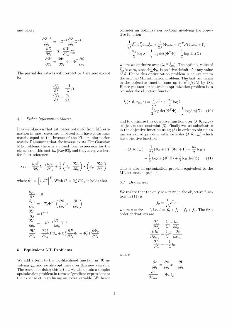
4.1 Derivatives

We will now derive the partial derivatives needed in orderto optimize the log-likelihood function in (9). We willdo these derivations term by term. To this end we writeL = f1 + f2 − f3 + f4, where

f1 =1

2λeTo Peo

f2 =no2

log λ

f3 =1

2log detW

f4 =1

2log detZ

where eo = Φoxo + Γ, and where W = ΦTΦ. Then itfollows that

∂f1

∂θk=

1

λeTo P

∂eo∂θk

+1

2λeTo

∂P

∂θkeo

∂f2

∂θk= 0

∂f3

∂θk=

1

2W−1 • ∂W

∂θk∂f4

∂θk=

1

2Z−1 • ∂Z

∂θk

where∂eo∂θk

=∂Φo∂θk

xo +∂Γ

∂θkwhere

∂P

∂θk=

∂

∂θk

(I − ΦmZ

−1ΦTm)

= −∂Φm∂θk

Z−1ΦTm

− Φm∂Z−1

∂θkΦTm − ΦmZ

−1 ∂ΦTm∂θk

3

and where

∂Z−1

∂θk= −Z−1 ∂Z

∂θkZ−1

∂Z

∂θk= Tm

∂W

∂θkTTm

∂W

∂θk=∂ΦT

∂θkΦ + ΦT

∂Φ

∂θk

The partial derivatives with respect to λ are zero exceptfor

∂f1

∂λ=−1

λf1

∂f2

∂λ=no2λ

4.2 Fisher Information Matrix

It is well-known that estimates obtained from ML esti-mation in most cases are unbiased and have covariancematrix equal to the inverse of the Fisher informationmatrix I assuming that the inverse exists. For GaussianML-problems there is a closed form expression for theelements of this matrix, [Kay93], and they are given herefor short reference

Ik,l =∂µTo∂θk

Σ−1o

∂µo∂θk

+1

2

(Σ−1o

∂Σo∂θk

)•(

Σ−1o

∂Σo∂θl

)

where θT =[λ θT

]T. With U = ΦTo PΦo it holds that

∂µo∂λ

= 0

∂µo∂θk

= −ToΦ−1

(∂Φ

∂θkµ+

∂Γ

∂θk

)∂Σo∂λ

= U−1

∂Σo∂θk

= −λU−1 ∂U

∂θkU−1

∂U

∂θk=∂ΦTo∂θk

PΦo + ΦTo∂P

∂θkΦo + ΦTo P

∂Φo∂θk

5 Equivalent ML Problems

We add a term to the log-likelihood function in (9) in-

volving ξm and we also optimize over this new variable.The reason for doing this is that we will obtain a simpleroptimization problem in terms of gradient expressions atthe expense of introducing an extra variable. We hence

consider an optimization problem involving the objec-tive function

1

2λξTmΦTmΦmξm +

1

2λ(Φoxo + Γ)TP (Φoxo + Γ)

+no2

log λ− 1

2log det(ΦTΦ) +

1

2log det(Z)

where we optimize over (λ, θ, ξm). The optimal value of

ξm is zero, since ΦTmΦm is positive definite for any valueof θ. Hence this optimization problem is equivalent tothe original ML estimation problem. The first two termsin the objective function sum up to eT e/(2λ) by (8).Hence yet another equivalent optimization problem is toconsider the objective function

lc(λ, θ, xm, e) =1

2λeT e+

no2

log λ

− 1

2log det(ΦTΦ) +

1

2log det(Z) (10)

and to optimize this objective function over (λ, θ, xm, e)subject to the constraint (3). Finally we can substitute ein the objective function using (3) in order to obtain anunconstrained problem with variables (λ, θ, xm) whichhas objective function

l(λ, θ, xm) =1

2λ(Φx+ Γ)T (Φx+ Γ) +

no2

log λ

− 1

2log det(ΦTΦ) +

1

2log det(Z) (11)

This is also an optimization problem equivalent to theML estimation problem.

5.1 Derivatives

We realize that the only new term in the objective func-tion in (11) is

f0 =1

2λeT e

where e = Φx + Γ, i.e. l = f0 + f2 − f3 + f4. The firstorder derivatives are

∂f0

∂θk=

1

λeT

∂e

∂θk∂f0

∂xmk

=1

λeT

∂e

∂xmk

∂f0

∂λ= − 1

λf0

where

∂e

∂θk=∂Φ

∂θkx+

∂Γ

∂θk∂e

∂xmk

= (Φm)k

4

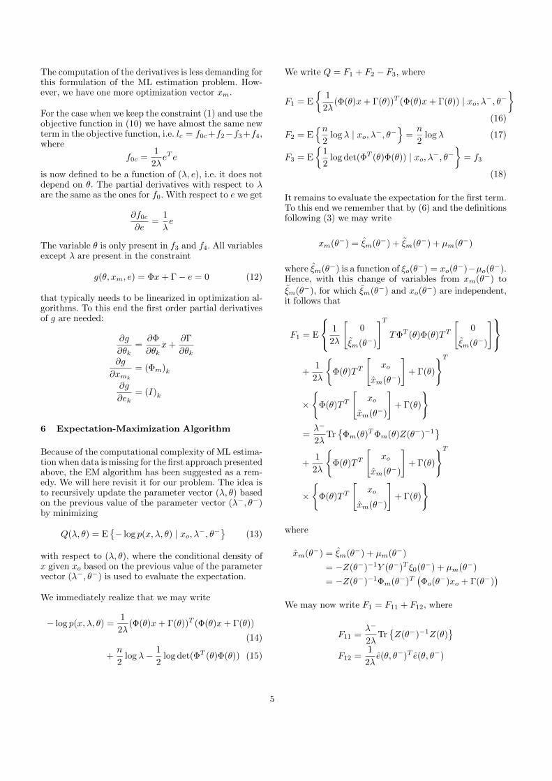
The computation of the derivatives is less demanding forthis formulation of the ML estimation problem. How-ever, we have one more optimization vector xm.

For the case when we keep the constraint (1) and use theobjective function in (10) we have almost the same newterm in the objective function, i.e. lc = f0c+f2−f3 +f4,where

f0c =1

2λeT e

is now defined to be a function of (λ, e), i.e. it does notdepend on θ. The partial derivatives with respect to λare the same as the ones for f0. With respect to e we get

∂f0c

∂e=

1

λe

The variable θ is only present in f3 and f4. All variablesexcept λ are present in the constraint

g(θ, xm, e) = Φx+ Γ− e = 0 (12)

that typically needs to be linearized in optimization al-gorithms. To this end the first order partial derivativesof g are needed:

∂g

∂θk=∂Φ

∂θkx+

∂Γ

∂θk∂g

∂xmk

= (Φm)k

∂g

∂ek= (I)k

6 Expectation-Maximization Algorithm

Because of the computational complexity of ML estima-tion when data is missing for the first approach presentedabove, the EM algorithm has been suggested as a rem-edy. We will here revisit it for our problem. The idea isto recursively update the parameter vector (λ, θ) basedon the previous value of the parameter vector (λ−, θ−)by minimizing

Q(λ, θ) = E{− log p(x, λ, θ) | xo, λ−, θ−

}(13)

with respect to (λ, θ), where the conditional density ofx given xo based on the previous value of the parametervector (λ−, θ−) is used to evaluate the expectation.

We immediately realize that we may write

− log p(x, λ, θ) =1

2λ(Φ(θ)x+ Γ(θ))T (Φ(θ)x+ Γ(θ))

(14)

+n

2log λ− 1

2log det(ΦT (θ)Φ(θ)) (15)

We write Q = F1 + F2 − F3, where

F1 = E

{1

2λ(Φ(θ)x+ Γ(θ))T (Φ(θ)x+ Γ(θ)) | xo, λ−, θ−

}(16)

F2 = E{n

2log λ | xo, λ−, θ−

}=n

2log λ (17)

F3 = E

{1

2log det(ΦT (θ)Φ(θ)) | xo, λ−, θ−

}= f3

(18)

It remains to evaluate the expectation for the first term.To this end we remember that by (6) and the definitionsfollowing (3) we may write

xm(θ−) = ξm(θ−) + ξm(θ−) + µm(θ−)

where ξm(θ−) is a function of ξo(θ−) = xo(θ

−)−µo(θ−).Hence, with this change of variables from xm(θ−) to

ξm(θ−), for which ξm(θ−) and xo(θ−) are independent,

it follows that

F1 = E

1

2λ

[0

ξm(θ−)

]TTΦT (θ)Φ(θ)TT

[0

ξm(θ−)

]+

1

2λ

{Φ(θ)TT

[xo

xm(θ−)

]+ Γ(θ)

}T

×

{Φ(θ)TT

[xo

xm(θ−)

]+ Γ(θ)

}

=λ−

2λTr{

Φm(θ)TΦm(θ)Z(θ−)−1}

+1

2λ

{Φ(θ)TT

[xo

xm(θ−)

]+ Γ(θ)

}T

×

{Φ(θ)TT

[xo

xm(θ−)

]+ Γ(θ)

}

where

xm(θ−) = ξm(θ−) + µm(θ−)

= −Z(θ−)−1Y (θ−)T ξ0(θ−) + µm(θ−)

= −Z(θ−)−1Φm(θ−)T(Φo(θ

−)xo + Γ(θ−))

We may now write F1 = F11 + F12, where

F11 =λ−

2λTr{Z(θ−)−1Z(θ)

}F12 =

1

2λe(θ, θ−)T e(θ, θ−)

5

and where

x(θ−) =

[xo

xm(θ−)

]e(θ, θ−) = Φ(θ)TT x(θ−) + Γ(θ)

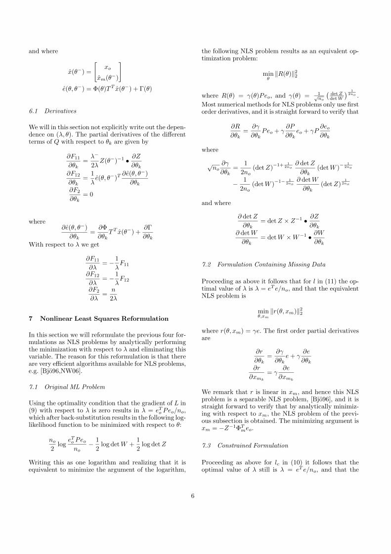
6.1 Derivatives

We will in this section not explicitly write out the depen-dence on (λ, θ). The partial derivatives of the differentterms of Q with respect to θk are given by

∂F11

∂θk=λ−

2λZ(θ−)−1 • ∂Z

∂θk∂F12

∂θk=

1

λe(θ, θ−)T

∂e(θ, θ−)

∂θk∂F2

∂θk= 0

where∂e(θ, θ−)

∂θk=∂Φ

∂θkTT x(θ−) +

∂Γ

∂θkWith respect to λ we get

∂F11

∂λ= − 1

λF11

∂F12

∂λ= − 1

λF12

∂F2

∂λ=

n

2λ

7 Nonlinear Least Squares Reformulation

In this section we will reformulate the previous four for-mulations as NLS problems by analytically performingthe minimization with respect to λ and eliminating thisvariable. The reason for this reformulation is that thereare very efficient algorithms available for NLS problems,e.g. [Bjo96,NW06].

7.1 Original ML Problem

Using the optimality condition that the gradient of L in(9) with respect to λ is zero results in λ = eTo Peo/no,which after back-substitution results in the following log-likelihood function to be minimized with respect to θ:

no2

logeTo Peono

− 1

2log detW +

1

2log detZ

Writing this as one logarithm and realizing that it isequivalent to minimize the argument of the logarithm,

the following NLS problem results as an equivalent op-timization problem:

minθ‖R(θ)‖22

where R(θ) = γ(θ)Peo, and γ(θ) = 1√no

(detZdetW

) 12no .

Most numerical methods for NLS problems only use firstorder derivatives, and it is straight forward to verify that

∂R

∂θk=

∂γ

∂θkPeo + γ

∂P

∂θkeo + γP

∂eo∂θk

where

√no

∂γ

∂θk=

1

2no(detZ)

−1+ 12no

∂ detZ

∂θk(detW )

− 12no

− 1

2no(detW )

−1− 12no

∂ detW

∂θk(detZ)

12no

and where

∂ detZ

∂θk= detZ × Z−1 • ∂Z

∂θk∂ detW

∂θk= detW ×W−1 • ∂W

∂θk

7.2 Formulation Containing Missing Data

Proceeding as above it follows that for l in (11) the op-timal value of λ is λ = eT e/no, and that the equivalentNLS problem is

minθ,xm

‖r(θ, xm)‖22

where r(θ, xm) = γe. The first order partial derivativesare

∂r

∂θk=

∂γ

∂θke+ γ

∂e

∂θk∂r

∂xmk

= γ∂e

∂xmk

We remark that r is linear in xm, and hence this NLSproblem is a separable NLS problem, [Bjo96], and it isstraight forward to verify that by analytically minimiz-ing with respect to xm, the NLS problem of the previ-ous subsection is obtained. The minimizing argument isxm = −Z−1ΦTmeo.

7.3 Constrained Formulation

Proceeding as above for lc in (10) it follows that theoptimal value of λ still is λ = eT e/no, and that the

6

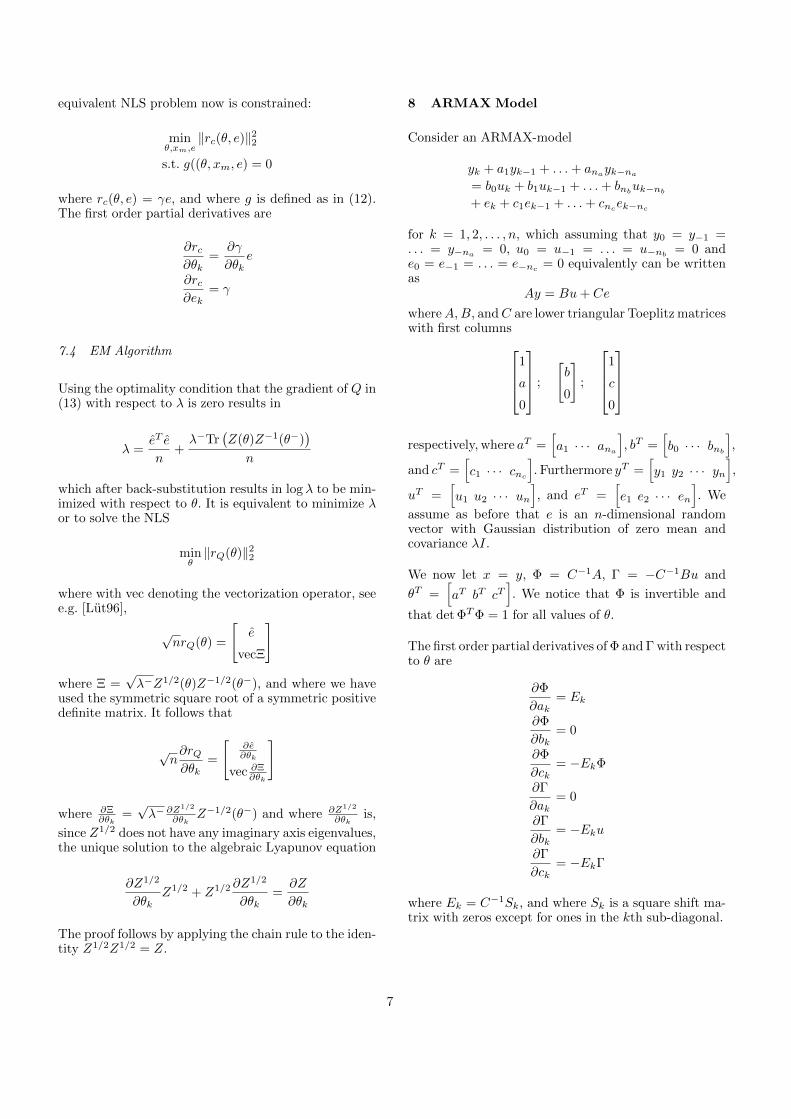
equivalent NLS problem now is constrained:

minθ,xm,e

‖rc(θ, e)‖22

s.t. g((θ, xm, e) = 0

where rc(θ, e) = γe, and where g is defined as in (12).The first order partial derivatives are

∂rc∂θk

=∂γ

∂θke

∂rc∂ek

= γ

7.4 EM Algorithm

Using the optimality condition that the gradient of Q in(13) with respect to λ is zero results in

λ =eT e

n+λ−Tr

(Z(θ)Z−1(θ−)

)n

which after back-substitution results in log λ to be min-imized with respect to θ. It is equivalent to minimize λor to solve the NLS

minθ‖rQ(θ)‖22

where with vec denoting the vectorization operator, seee.g. [Lut96],

√nrQ(θ) =

[e

vecΞ

]

where Ξ =√λ−Z1/2(θ)Z−1/2(θ−), and where we have

used the symmetric square root of a symmetric positivedefinite matrix. It follows that

√n∂rQ∂θk

=

[∂e∂θk

vec ∂Ξ∂θk

]

where ∂Ξ∂θk

=√λ− ∂Z

1/2

∂θkZ−1/2(θ−) and where ∂Z1/2

∂θkis,

since Z1/2 does not have any imaginary axis eigenvalues,the unique solution to the algebraic Lyapunov equation

∂Z1/2

∂θkZ1/2 + Z1/2 ∂Z

1/2

∂θk=∂Z

∂θk

The proof follows by applying the chain rule to the iden-tity Z1/2Z1/2 = Z.

8 ARMAX Model

Consider an ARMAX-model

yk + a1yk−1 + . . .+ anayk−na

= b0uk + b1uk−1 + . . .+ bnbuk−nb

+ ek + c1ek−1 + . . .+ cncek−nc

for k = 1, 2, . . . , n, which assuming that y0 = y−1 =. . . = y−na

= 0, u0 = u−1 = . . . = u−nb= 0 and

e0 = e−1 = . . . = e−nc= 0 equivalently can be written

asAy = Bu+ Ce

whereA,B, andC are lower triangular Toeplitz matriceswith first columns

1

a

0

;

[b

0

];

1

c

0

respectively, where aT =

[a1 · · · ana

], bT =

[b0 · · · bnb

],

and cT =[c1 · · · cnc

]. Furthermore yT =

[y1 y2 · · · yn

],

uT =[u1 u2 · · · un

], and eT =

[e1 e2 · · · en

]. We

assume as before that e is an n-dimensional randomvector with Gaussian distribution of zero mean andcovariance λI.

We now let x = y, Φ = C−1A, Γ = −C−1Bu and

θT =[aT bT cT

]. We notice that Φ is invertible and

that det ΦTΦ = 1 for all values of θ.

The first order partial derivatives of Φ and Γ with respectto θ are

∂Φ

∂ak= Ek

∂Φ

∂bk= 0

∂Φ

∂ck= −EkΦ

∂Γ

∂ak= 0

∂Γ

∂bk= −Eku

∂Γ

∂ck= −EkΓ

where Ek = C−1Sk, and where Sk is a square shift ma-trix with zeros except for ones in the kth sub-diagonal.

7

9 Numerical Implementation

The first four formulations of the ML estimation prob-lem suffer from numerical difficulties, and we will presentno results regarding their performance. For the last fourformulations, which are all NLS formulations, we haveimplemented two of them, see below for motivation.The numerical implementation has been carried out inMatlab using its optimization toolbox with the func-tion lsqnonlin, which implements a NLS algorithmusing first order derivatives only. This is a standardapproach in system identification, see e.g. [Lju99]. Wehave used the trust-region-reflective option. See [Bjo96]and the references therein for more details on differenttypes of NLS algorithms. The following tolerances fortermination have been used for the method described inSection 7.1, which we from now on call the variable pro-jection method: TolFun = 10−15 and TolX = 10−5/

√q.

There are many other codes available than the one inthe Matlab optimization toolbox. It should also be men-tioned that there is a potential to obtain faster conver-gence and better numerical behavior by utilizing spe-cial purpose codes for separable NLS problems, see e.g.the survey [GP03] and the references therein. Becauseof this we have used the so-called Kaufman search direc-tion when implementing the variable projection methodin Section 7.1. This avoids computing the exact partialderivatives of P , which are the most costly derivatives tocompute. According to [GP03] this is the best choice forseparable NLS problems, and it also outperforms the for-mulation in Section 7.2 which does not need to computethe partial derivatives of P . In the appendix we showhow the Kaufman search direction can be implementedin any standard NLS solver. It is actually possible to in-terpret the Kaufman search direction for the method inSection 7.1 as a block coordinate descent method for themethod in Section 7.2 where at each iteration a descentstep is taken in the θ-direction and an exact minimiza-tion is performed in the xm-direction. This is the reasonwhy the Kaufman search direction is preferable, [Par85].To summarize, it can be interpreted either as an approx-imation of the gradient for the method in Section 7.1, seethe appendix, or as an efficient block-coordinate methodfor the method in Section 7.2.

The EM method in Section 7.4 is often proposed as agood method to use when data is missing, but it is ingeneral not very fast unless it is possible to solve theminimization step quickly. For certain problems thereare closed form solutions, [Isa93]. In our case this is nottrue in general. However, it is not necessary to performthe minimization step to very high accuracy. It is oftensufficient to just obtain a decrease in Q. These type ofalgorithms are usually called generalized EM algorithms,e.g. [MK08]. Here we will employ such an algorithm foroptimizing Q by running two iterations of lsqnonlinfor the first five iterations in the EM algorithm, and

thereafter running one iteration. The overall terminationcriteria for the EM method is ‖θ − θ−‖2 ≤ 10−5/

√q.

We have not considered to implement the constrainedformulation of the NLS problem in Section 7.3. Thiscould potentially be a good candidate, especially for theapplication to ARMAX models in case the constraint ismultiplied with C, since then the constraint will becomebilinear in the variables. In addition to this the deriva-tives with respect to the objective function and the con-straints are very simple. However, the application of con-strained NLS for black box identification in [VMSVD10]does not show that it is advantageous with respect tocomputational speed for that application. However, ithas the advantage that it can address unstable models.

The computational complexity in terms of flop count periteration for computing the gradients is for all algorithmsof the same order. This is the most time-consuming partof an iteration. The flop count is linear in the numberof parameters q, quadratic in the underlying numberof data n, and cubical in the number of missing datanm = n− no. It should me mentioned that for the AR-MAX model it is possible to make use of the Toeplitzstructure of A, B, and C to decrease the computationaltime for the partial derivatives of Φ and Γ. Furtherspeedup can be obtained by changing the order in whichthe computations are performed. This is not within thescope of this work and is left for future research.

10 Examples

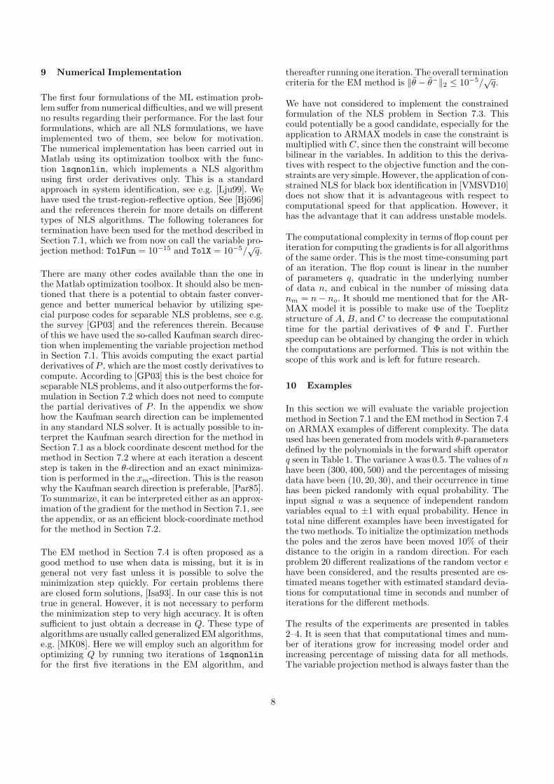
In this section we will evaluate the variable projectionmethod in Section 7.1 and the EM method in Section 7.4on ARMAX examples of different complexity. The dataused has been generated from models with θ-parametersdefined by the polynomials in the forward shift operatorq seen in Table 1. The variance λ was 0.5. The values of nhave been (300, 400, 500) and the percentages of missingdata have been (10, 20, 30), and their occurrence in timehas been picked randomly with equal probability. Theinput signal u was a sequence of independent randomvariables equal to ±1 with equal probability. Hence intotal nine different examples have been investigated forthe two methods. To initialize the optimization methodsthe poles and the zeros have been moved 10% of theirdistance to the origin in a random direction. For eachproblem 20 different realizations of the random vector ehave been considered, and the results presented are es-timated means together with estimated standard devia-tions for computational time in seconds and number ofiterations for the different methods.

The results of the experiments are presented in tables2–4. It is seen that that computational times and num-ber of iterations grow for increasing model order andincreasing percentage of missing data for all methods.The variable projection method is always faster than the

8

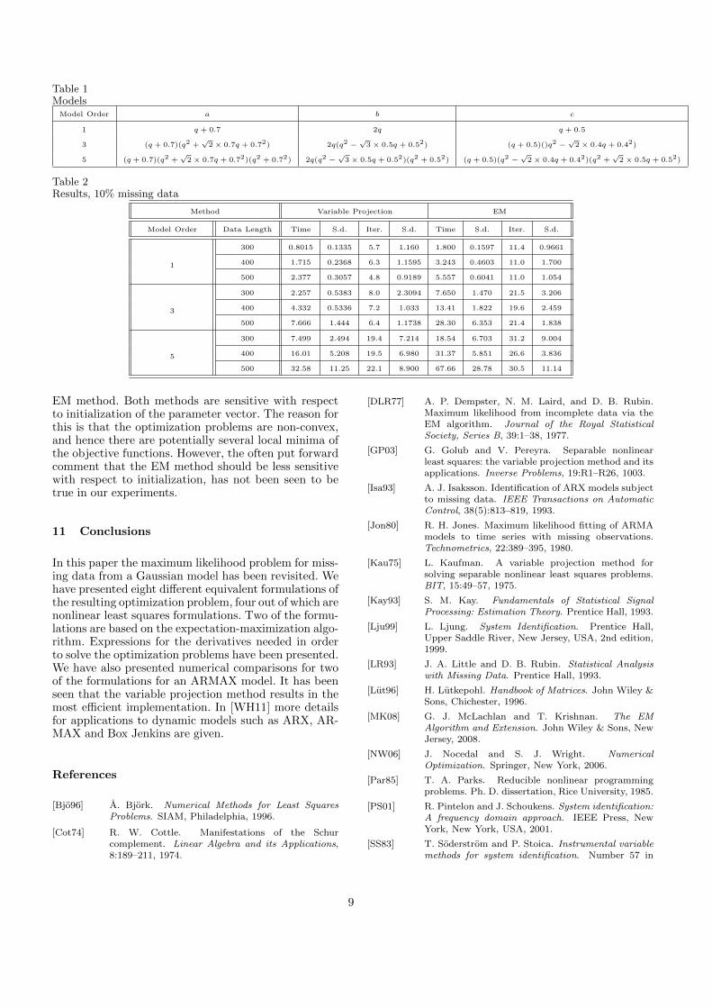
Table 1ModelsModel Order a b c

1 q + 0.7 2q q + 0.5

3 (q + 0.7)(q2 +√2× 0.7q + 0.72) 2q(q2 −

√3× 0.5q + 0.52) (q + 0.5)()q2 −

√2× 0.4q + 0.42)

5 (q + 0.7)(q2 +√2× 0.7q + 0.72)(q2 + 0.72) 2q(q2 −

√3× 0.5q + 0.52)(q2 + 0.52) (q + 0.5)(q2 −

√2× 0.4q + 0.42)(q2 +

√2× 0.5q + 0.52)

Table 2Results, 10% missing data

Method Variable Projection EM

Model Order Data Length Time S.d. Iter. S.d. Time S.d. Iter. S.d.

1

300 0.8015 0.1335 5.7 1.160 1.800 0.1597 11.4 0.9661

400 1.715 0.2368 6.3 1.1595 3.243 0.4603 11.0 1.700

500 2.377 0.3057 4.8 0.9189 5.557 0.6041 11.0 1.054

3

300 2.257 0.5383 8.0 2.3094 7.650 1.470 21.5 3.206

400 4.332 0.5336 7.2 1.033 13.41 1.822 19.6 2.459

500 7.666 1.444 6.4 1.1738 28.30 6.353 21.4 1.838

5

300 7.499 2.494 19.4 7.214 18.54 6.703 31.2 9.004

400 16.01 5.208 19.5 6.980 31.37 5.851 26.6 3.836

500 32.58 11.25 22.1 8.900 67.66 28.78 30.5 11.14

EM method. Both methods are sensitive with respectto initialization of the parameter vector. The reason forthis is that the optimization problems are non-convex,and hence there are potentially several local minima ofthe objective functions. However, the often put forwardcomment that the EM method should be less sensitivewith respect to initialization, has not been seen to betrue in our experiments.

11 Conclusions

In this paper the maximum likelihood problem for miss-ing data from a Gaussian model has been revisited. Wehave presented eight different equivalent formulations ofthe resulting optimization problem, four out of which arenonlinear least squares formulations. Two of the formu-lations are based on the expectation-maximization algo-rithm. Expressions for the derivatives needed in orderto solve the optimization problems have been presented.We have also presented numerical comparisons for twoof the formulations for an ARMAX model. It has beenseen that the variable projection method results in themost efficient implementation. In [WH11] more detailsfor applications to dynamic models such as ARX, AR-MAX and Box Jenkins are given.

References

[Bjo96] A. Bjork. Numerical Methods for Least SquaresProblems. SIAM, Philadelphia, 1996.

[Cot74] R. W. Cottle. Manifestations of the Schurcomplement. Linear Algebra and its Applications,8:189–211, 1974.

[DLR77] A. P. Dempster, N. M. Laird, and D. B. Rubin.Maximum likelihood from incomplete data via theEM algorithm. Journal of the Royal StatisticalSociety, Series B, 39:1–38, 1977.

[GP03] G. Golub and V. Pereyra. Separable nonlinearleast squares: the variable projection method and itsapplications. Inverse Problems, 19:R1–R26, 1003.

[Isa93] A. J. Isaksson. Identification of ARX models subjectto missing data. IEEE Transactions on AutomaticControl, 38(5):813–819, 1993.

[Jon80] R. H. Jones. Maximum likelihood fitting of ARMAmodels to time series with missing observations.Technometrics, 22:389–395, 1980.

[Kau75] L. Kaufman. A variable projection method forsolving separable nonlinear least squares problems.BIT, 15:49–57, 1975.

[Kay93] S. M. Kay. Fundamentals of Statistical SignalProcessing: Estimation Theory. Prentice Hall, 1993.

[Lju99] L. Ljung. System Identification. Prentice Hall,Upper Saddle River, New Jersey, USA, 2nd edition,1999.

[LR93] J. A. Little and D. B. Rubin. Statistical Analysiswith Missing Data. Prentice Hall, 1993.

[Lut96] H. Lutkepohl. Handbook of Matrices. John Wiley &Sons, Chichester, 1996.

[MK08] G. J. McLachlan and T. Krishnan. The EMAlgorithm and Extension. John Wiley & Sons, NewJersey, 2008.

[NW06] J. Nocedal and S. J. Wright. NumericalOptimization. Springer, New York, 2006.

[Par85] T. A. Parks. Reducible nonlinear programmingproblems. Ph. D. dissertation, Rice University, 1985.

[PS01] R. Pintelon and J. Schoukens. System identification:A frequency domain approach. IEEE Press, NewYork, New York, USA, 2001.

[SS83] T. Soderstrom and P. Stoica. Instrumental variablemethods for system identification. Number 57 in

9

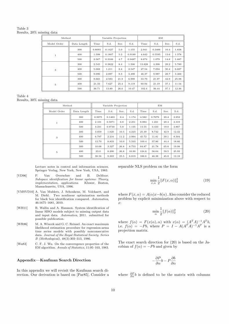
Table 3Results, 20% missing data

Method Variable Projection EM

Model Order Data Length Time S.d. Iter. S.d. Time S.d. Iter. S.d.

1

300 0.8093 0.1427 5.0 1.155 2.941 0.3466 16.4 1.838

400 1.598 0.1807 5.2 0.9189 4.642 0.5595 13.6 1.578

500 2.567 0.3166 4.7 0.9487 8.674 1.079 14.8 1.687

3

300 2.545 0.3822 8.4 1.506 13.828 4.398 29.2 5.789

400 5.068 1.211 8.4 2.547 27.54 7.094 30.4 6.687

500 9.096 2.887 8.3 3.498 46.37 9.987 28.7 3.466

5

300 8.665 2.583 21.9 6.999 33.79 21.97 42.9 25.98

400 21.33 7.627 25.4 9.119 60.94 21.19 37.1 11.54

500 36.71 13.89 26.0 10.47 102.4 36.44 37.1 12.36

Table 4Results, 30% missing data

Method Variable Projection EM

Model Order Data Length Time S.d. Iter. S.d. Time S.d. Iter. S.d.

1

300 0.9975 0.1463 6.4 1.174 4.582 0.7679 20.4 2.952

400 2.101 0.5871 6.8 2.251 8.884 1.221 20.4 2.319

500 3.231 0.9740 5.8 1.135 14.55 3.433 19.0 2.867

3

300 3.059 1.020 10.5 4.223 25.39 8.742 42.9 12.42

400 6.797 2.216 11.2 3.994 45.72 11.81 39.1 8.504

500 12.79 8.833 10.0 5.333 109.4 57.86 44.4 18.66

5

300 10.68 3.327 26.8 8.753 64.87 21.78 65.8 19.98

400 23.0 8.200 26.8 10.90 124.8 56.64 59.5 25.93

500 38.56 9.302 25.5 6.819 166.6 46.38 45.8 12.18

Lecture notes in control and information sciences.Springer Verlag, New York, New York, USA, 1983.

[VD96] P. Van Overschee and B. DeMoor.Subspace identification for linear systems: Theory,implementation, applications. Kluwer, Boston,Massachusetts, USA, 1996.

[VMSVD10] A. Van Mulders, J. Schoukens, M. Volckaert, andM. Diehl. Two nonlinear optimization methodsfor black box identification compared. Automatica,46:1675–1681, 2010.

[WH11] R. Wallin and A. Hansson. System identification oflinear SISO models subject to missing output dataand input data. Automatica, 2011. submitted forpossible publication.

[WR86] M. A. Wincek and G. C. Reinsel. An exact maximumlikelihood estimation procedure for regression-armatime series models with possibly nonconsecutivedata. Journal of the Royal Statistical Society. SeriesB (Methodogical), 48(3):303–313, 1986.

[Wu83] C. F. J. Wu. On the converegence properties of theEM algorithm. Annals of Statistics, 11:95–103, 1983.

Appendix—Kaufman Search Direction

In this appendix we will revisit the Kaufman search di-rection. Our derivation is based on [Par85]. Consider a

separable NLS problem on the form

minx,α

1

2‖F (x, α)‖22 (19)

whereF (x, α) = A(α)x−b(α). Also consider the reducedproblem by explicit minimization above with respect tox:

minα

1

2‖f(α)‖22 (20)

where f(α) = F (x(α), α) with x(α) = (ATA)−1AT b,i.e. f(α) = −Pb, where P = I − A(ATA)−1AT is aprojection matrix.

The exact search direction for (20) is based on the Ja-cobian of f(α) = −Pb and given by

−∂P∂α

b− P ∂b

∂α

where ∂P∂α b is defined to be the matrix with columns

10

∂P∂αk

b. In this expression

∂P

∂αk= − ∂A

∂αk(ATA)−1AT

+A(ATA)−1

(∂AT

∂αkA+AT

∂A

∂αk

)(ATA)−1AT

−A(ATA)−1 ∂AT

∂αk

= −P ∂A

∂αk(ATA)−1AT −A(ATA)−1 ∂A

T

∂αkP

From this we conclude that the exact Jacobian is givenby

P∂A

∂α(ATA)−1AT b+A(ATA)−1 ∂A

T

∂αPb− P ∂b

∂α

The second term contains the factor Pb = −f(α), whichis small for values of α close to optimum, and this isthe term that is omitted in the approximation proposedby Kaufman, [Kau75]. In the original work this approxi-mation was suggested for the Gauss-Newton-Marquardtalgorithm. Here we have used it for a trust-region algo-rithm.

The detailed expression for our separable NLS problemfollows from making the following identifications: A =γΦm, b = −γeo, α = θ and x = xm, where the latter isa misuse of notation. It follows that P = I−ΦmZ

−1ΦTmas before. Moreover

∂A

∂αk=

∂γ

∂θkΦm + γ

∂Φm∂θk

∂b

∂αk= − ∂γ

∂θkeo − γ

∂eo∂θk

In addition to this we make use of that −(ATA)−1b isthe least squares solution of minxm

‖Φmxm+eo‖2. Thenthe Kaufman Jacobian can be efficiently computed fromthe above formulas as

−P(∂A

∂αxm +

∂b

∂α

)

11