Maximal Lifetime Scheduling in Sensor Surveillance Networks

Hai Liu1, Pengjun Wan2, Chih-Wei Yi2, Siaohua Jia1, Sam Makki3 and Niki Pissionou4

Dept of Computer Science 1City University of Hong Kong, 2Illinois Institute of TechnologyDept of Electrical Engineering & Computer Science 3University of ToledoTelecommunications & Information Technology Institute 4Florida International University

Infocom 2005

Outline

Introduction System model and problem statement Solutions Experiment and simulation Conclusions

Introduction One important characteristic of sensor networks is th

e stringent power budget of wireless sensor nodes. It is important to prolong the lifetime of sensor netw

orks. In this paper, we discuss a scheduling problem in sen

sor surveillance networks. Sensor surveillance networks

Given a set of sensors and targets in a Euclidean plane, all targets should be watched by sensors at any time

A sensor can watch only one target at a time

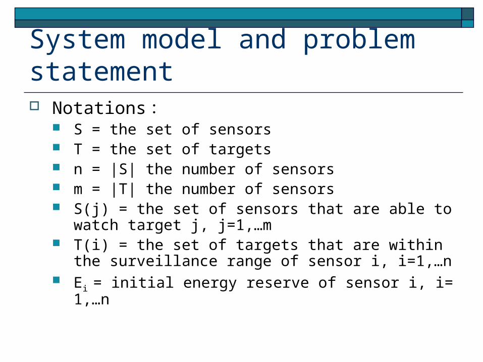
System model and problem statement Notations ：

S = the set of sensors T = the set of targets n = |S| the number of sensors m = |T| the number of sensors S(j) = the set of sensors that are able to watch target j, j=1,

…m T(i) = the set of targets that are within the surveillance ran

ge of sensor i, i=1,…n Ei = initial energy reserve of sensor i, i=1,…n

System model and problem statement There two requirements for sensors watching targets ：

Each sensor can watch at most one target at a time. Each target should be watched by one sensor at anytime.

The problem is to find a schedule that meets the above two requirements for sensors watching targets, such that lifetime is maximized.

Lifetime is defined as the length of time until there exists a target j such that all sensors in S(j) run out their energy.

Solutions Tackle the problem in three steps.

Step1, compute the upper bound on the maximal lifetime of the system and a workload matrix of sensors.

Step2, decompose the workload matrix into a sequence of schedule matrices.

Step3, obtain a target watching timetable for each sensor.

Find maximal lifetime Use linear programming technique to find the maxim

um lifetime of the system. L ： the lifetime of the surveillance system xij ： the total time sensor i watching target j

The maximum lifetime for sensors watching targets can be formulated ：

Find maximal lifetime Find a schedule for each sensor

The value of xij can be represented as a

workload matrix ：

There two important features about this matrix ： the sum of all elements in each column is equal to L （ fr

om eq.(1) ） the sum of all elements in each row is less than or equal to

L (from ieq(2))

Decompose workload matrix The lifetime can be divided into of a sequence of sessions. Thus

the schedule of sensors during a session can be represented as a matrix.

There is only one positive number in each column, and at most one positive number in each row.

All non-zero elements in this matrix have the same value. Decompose the workload matrix into a sequence of session sche

dule matrices ：

where zi , i=1,2,…,t ,is the length of time of session i.

A special case n=m

according eq.(1) and ineq.(2)

we have ：

combining (4) and (5), we have:

A special case n=m

(3) and (6) imply that the workload matrix the sum of each column is the same as the sum of each row, all equal to L.

divide the workload matrix Xnxm by L and denote the new matrix by Ynxn , that is, yij = xij / L, for i,j =1,2,…,n .

For matrix Ynxn , we have :

Matrix Ynxn is a Doubly Stochastic Matrix.

A special case n=m

when n=m ,workload matrix Xnxm can be decomposed into a sequence of matrices ：

(theorem 3 in [14] T. Inukai, “An Efficient SS/TDMA Time Slot Assignment Algorithm” Algorithm”, IEEE Trans.)

General case n>m

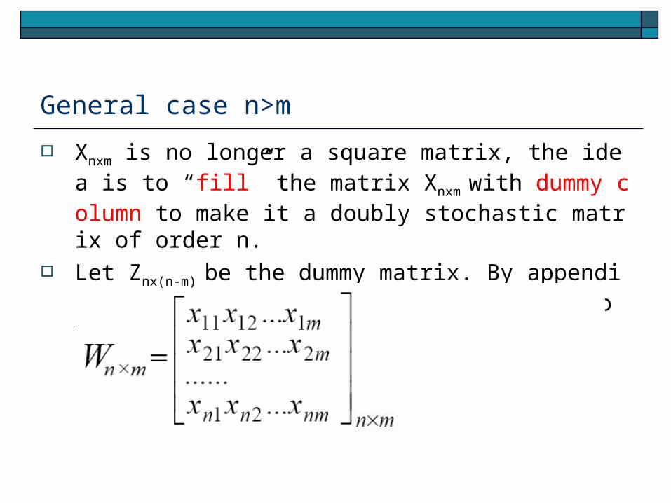
Xnxm is no longer a square matrix, the idea is to “fill” the matrix Xnxm with dummy column to make it a doubly stochastic matrix of order n.

Let Znx(n-m) be the dummy matrix. By appending the column of the dummy matrix to to the right hand side of Xnxm .

General case n>m

To make matrix Wnxn having the feature of (3) and (6), the dummy matrix Znx(n-m) should satisfy the following conditions ：

Let record the sum of the remaining undetermined element of row i and column j ,for i=1,…,n and j= 1,…,n-m

Initially,

General case n>m

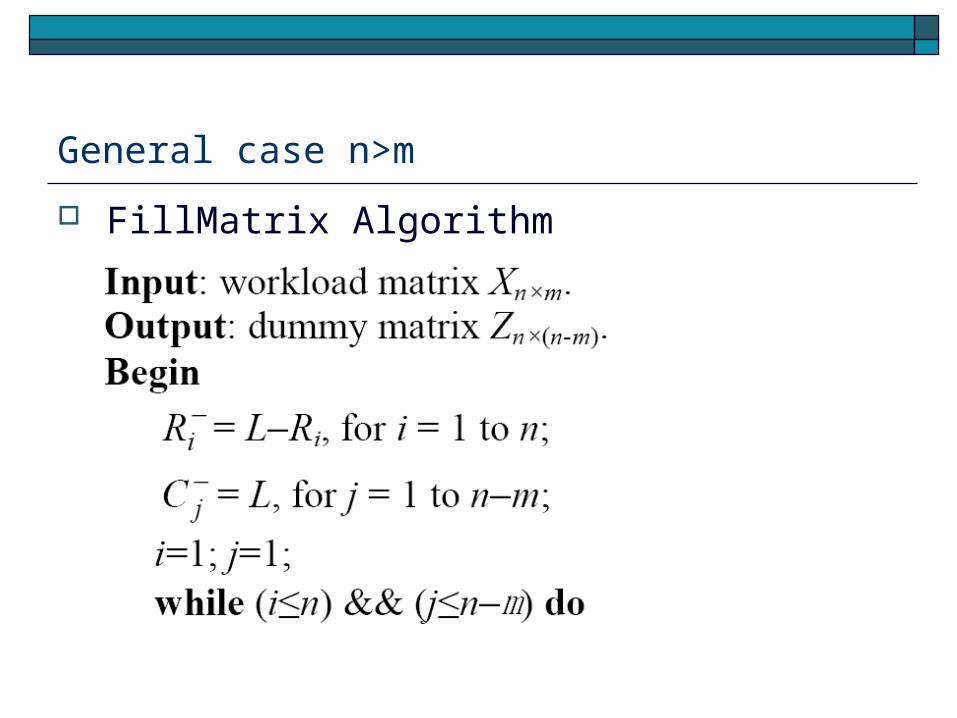
FillMatrix Algorithm

General case n>m FillMatrix Algorithm

If

If

00iR

0

0jC

General case n>m FillMatrix Algorithm

If ,we can determine elements in both row I and in column j by .

0

0

00iR

General case n>m FillMatrix Algorithm

Wnxn can be decomposed as ：

simply denote ciL as ci ,

Proof

General case n>m Let denote the matrix which contains the first m columns i

n ,i=1,…,t , we have

The matrices ,i=1,…,t, are the schedule matrices In session i, sensors are scheduled to watch their respective

targets according to the position of “1” elements in for the period of ci time.

Workload matrix is decomposable to a sequence of schedule matrices such that the optimal lifetime can be achieved.

Algorithm for decomposing workload matrix

The basic idea of the algorithm is to represent the filled workload matrix as a bipartite graph where one side are sensors and other are targets.

Decomposing the filled workload matrix is transformed into the problem of finding perfect matchings in a bipartite graph.

Proof

PerfectMatching algorithm M denote a set of edges of a perfect matching. M-path is a path in the bipartite graph. It starts with

a S node that not in M and end with a T node that is also not in M.

By replacing M-edges in the M-path by the non M-edge, the number of edges in M is incremented by 1.

Finding the M-path and increasing the size of M, until a perfect matching is found.

S T

S1

S5

S2

S4

S3

T1

T3

T2

T4

T5

M ： { （ S1,T 1 ） }

M-path ：

{ （ S2,T1 ）（ T1,S1 ）（ S1,T

2 ） }

PerfectMatching algorithm

M ： { （ S2,T1 ）（ S1,T2 ） }

DecomposeMatric Algorithm

DecomposeMatric Algorithm

Obtain schedule timetable

Simply take the i-th row of all the schedule matrices, and combine the time of the consecutive sessions that it watches the same target.

Then, we have an independent timetable for each sensor.

Experiment and Simulation Experiment

Place 6 sensors and 3 targets in a 50x50 two-dimensional free-space region.

The survelliance range is set to 20.(the solution can work for any system with non-uniform surveillance range)

The initial energy reserves of sensors are random number generated in the range of [0,50] with the mean at 25.

Experiment cont’

Step1, using the linear programming to compute the maximum lifetime and the workload matrix.

L ： 40.5643 hr.

Experiment cont’

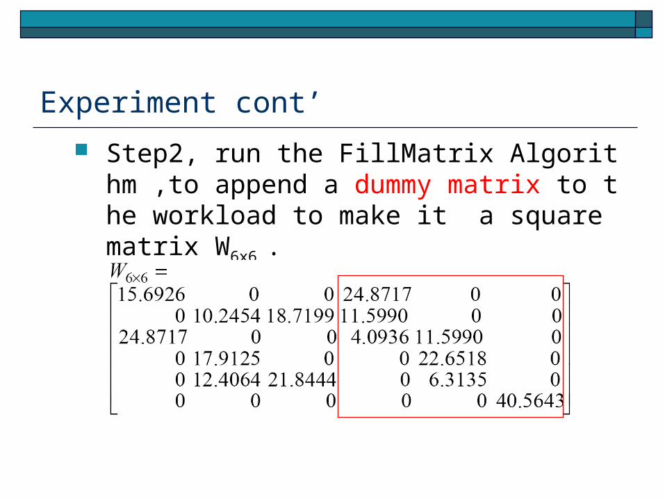
Step2, run the FillMatrix Algorithm ,to append a dummy matrix to the workload to make it a square matrix W6x6 .

Experiment cont’

Then, run the DecomposeMatrix Algorithm to decompose W6x6 into a sequence of schedule matrices , such that W6x6 =c1P1+c2P2+…+c5P5

By removing the dummy columns of the schedule matrices, we have:

Experiment cont’

Finally, obtain target watch timetables for sensors based on the above schedule matrix.

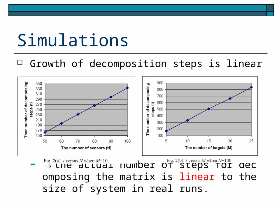
Simulations Growth of decomposition steps is linear

⇒the actual number of steps for decomposing the matrix is linear to the size of system in real runs.

Simulations cont’ Comparison with a greedy method （ surveillance ra

nge ） Set N=100

and M=10

Simulations cont’ Comparison with a greedy method （ sensor densit

y ）

Conclusions Solution consists of three steps:

compute the maximal lifetime of the system and a workload matrix by using linear programming method.

decompose the workload matrix into a sequence of schedule matrices by using perfect matching method.

obtain target watching timetable for sensors. The solution is the optimum in the sense that it can find the sc

hedules that achieve the maximum lifetime. the steps of decomposition is linear to the size of system. This method can take more advantages in the situtation that s

enses are densely deployed or sensors have larger coverage ranges.

Theorem 3

Theorem 5

konig

Konig theorem The number of edges in a maximum matching

of a bipartite graph G=(X,Y,E) is equal to

|X|-σ(G), where σ(G) is the deficiency of G.