Maverick Woo August 2002 / CMU The Discrepancy Method An Introduction Using Minimum Spanning Trees.
133
August 2002 / CMU Maverick Maverick Woo Woo The Discrepancy Method The Discrepancy Method An Introduction Using Minimum Spanning Trees
-
Upload
sylvia-nichols -
Category
Documents
-
view
216 -
download
1
Transcript of Maverick Woo August 2002 / CMU The Discrepancy Method An Introduction Using Minimum Spanning Trees.

August 2002 / CMU
Maverick Maverick WooWoo
The Discrepancy MethodThe Discrepancy Method
An Introduction UsingMinimum Spanning Trees

2
Did you know?Did you know?
“Recursion comes from the verb recur. There is no verb recurse.”
http://www.cse.ucsc.edu/~larrabee/ce185/reader/node191.html

3
Did you know?Did you know?
If m/n = (logO(1) n), then (m, n) = O(1).
Linear-Time Pointer-Machine Algorithms for Least Common Ancestors, MST Verification and Dominators
by Buchsbaum, Kaplan, Rogers and Westbrook

4
CreditCredit
The Discrepancy MethodBernard Chazelle
5
CreditCredit
Finding MST in O(m(m,n)) TimeSeth Pettie
6
The Discrepancy MethodThe Discrepancy Method
MinimumFinding

7
Minimum FindingMinimum Finding
For boys and girls:
Given an unsorted array A of n unique integers, find the minimum.

8
One Possible AlgorithmOne Possible Algorithm
Divide A into 100 parts.
For each part, recursively find the minimum within that part.
Find the minimum among the 100 minimum elements from each part.

9
A Term To IntroduceA Term To Introduce
Those 100 elements obtained from recursion form a
low discrepancy subset.

10
"Definition""Definition"
Roughly speaking, a low discrepancy subset is a subset that is
representative,
i.e. (we hope) the solution of the problem using this subset is “close to” the solution using the original set.

11
One Possible AlgorithmOne Possible Algorithm
Divide A into 100 parts.
For each part, recursively findthe minimum within that part.
Find the minimum among the 100 minimum elements from each part.

12
About SizeAbout Size
How big should the low discrepancy subset be?
We could have divide A into100 partslog(n) partsn/5 parts

13
Let's Try SamplingLet's Try Sampling
Sample u.a.r. 1% of the elements.
Recursively find their minimum x.
Reject elements larger than x.
What is the expected number of elements to remain?
100k/(k+1) ~= 100100k/(k+1) ~= 100

14
"Close To" ???"Close To" ???
These 1% of the elements also form a low discrepancy subset.
Their minimum is “close to” the true minimum.

15
The Discrepancy MethodThe Discrepancy Method
MedianFinding

16
Median FindingMedian Finding
For adults:
Given an unsorted array A of n unique integers, find the median.

17
A Randomized AlgorithmA Randomized Algorithm
Pick a pivot element such that it splits A into a (¼, ¾) split (or even better).
Recur on the correct side.

18
A Deterministic AlgorithmA Deterministic Algorithm
Divide A into groups of 5.Find the median of each group.Recursively find the median x of these medians and use x to pivot, then recur.
How far away is x from the true median?

19
Answer: Not FarAnswer: Not Far
… …
… …
… x …
… …
… …

20
Answer: Not FarAnswer: Not Far
… …
… …
… x …
… …
… …

21
A Deterministic AlgorithmA Deterministic Algorithm
Divide A into groups of 5.Find the median of each group.Recursively find the median x of these medians and use x to pivot, then recur.
How far away is x from the true median?
What is the low
discrepancy subset here?
What is the low
discrepancy subset here?

23
The Discrepancy MethodThe Discrepancy Method
Identify a low discrepancy subset.
Solve the problem using it (probably with divide-and-conquer).
Patch the almost-right solution to obtain the surely-right solution.

24
About SizeAbout Size
How big should the low discrepancy subset be?
We could have divide A into100 partslog(n) partsn/5 parts

25
Trade-offTrade-off
Biggersubset
Lower discrepancy
Less work to patch solution
More time to get a solution
Doesn’t seem to have aneasy answer. Be creative!

26
A Lossy Data StructureA Lossy Data Structure
Soft Heaps

27
Soft HeapsSoft Heaps
Items with keys from a total order
create(S)delete(S, x)findmin(S)meld(S, S’)insert(S, x)
Amortized O(1)
O(log 1/)

28
The CatchThe Catch
Soft heaps can corrupt the keys!
Consider a mixed sequence of operations that includes n inserts.For any error rate 0 < · ½, a soft heap can contain at most n corrupted keys at a time.

29
Key CorruptionKey Corruption
The values of certain keys can be increased at the sole discretion of the soft heap.
Once corrupted, a key will remain corrupted.

30
Even WorseEven Worse
When you delete a (corrupted) key, some other keys may be corrupted during the deletion.
It is possible for all keys to become corrupted over the lifetime of the soft heap.

31
The WorstThe Worst
Because of deletions, the proportion of corrupted items inside a soft heap could be much greater than .
(The theorem says “in a mixed sequence of operations that includes n inserts…”.)
32
Median Once MoreMedian Once More
1. Pick be ¼.
2. Insert n integers.
3. Do n/2 findmins, each followed by a deletion.
Among the keys deleted, how far away is the largest original key
from the true median?
Note itsonline nature.
Note itsonline nature.

33
Answer: Not FarAnswer: Not Far
We have n/2 elements left. At most n/4 of them are corrupted.
The worst case is when those n/4 elements were small in the beginning.
So the largest original key we deleted is at most rank 3n/4. Now pivot!
34
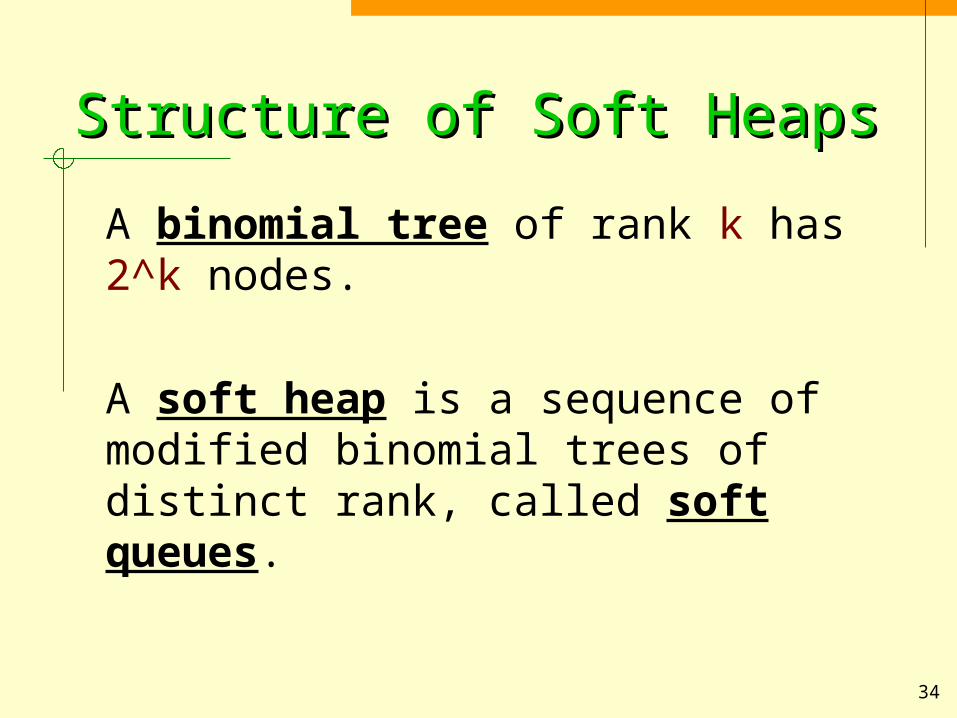
Structure of Soft HeapsStructure of Soft Heaps
A binomial tree of rank k has 2^k nodes.
A soft heap is a sequence of modified binomial trees of distinct rank, called soft queues.

35
Soft QueuesSoft Queues
A binomial tree with possibly a few sub-tree pruned.The rank of a node is the number of children in the original tree. (Hence it’s an upper bound.)Rank invariant: The root has at least brank(root)/2c children.

36
Item ListsItem Lists
A node contains an item list.ckey is the common value of all keys in the list (upper bound of all keys).A soft queue is heap-ordered w.r.t. ckeys.Let r = 2dlog 1/e + 2. We require all corrupted items stored at nodes of rank > r.
37
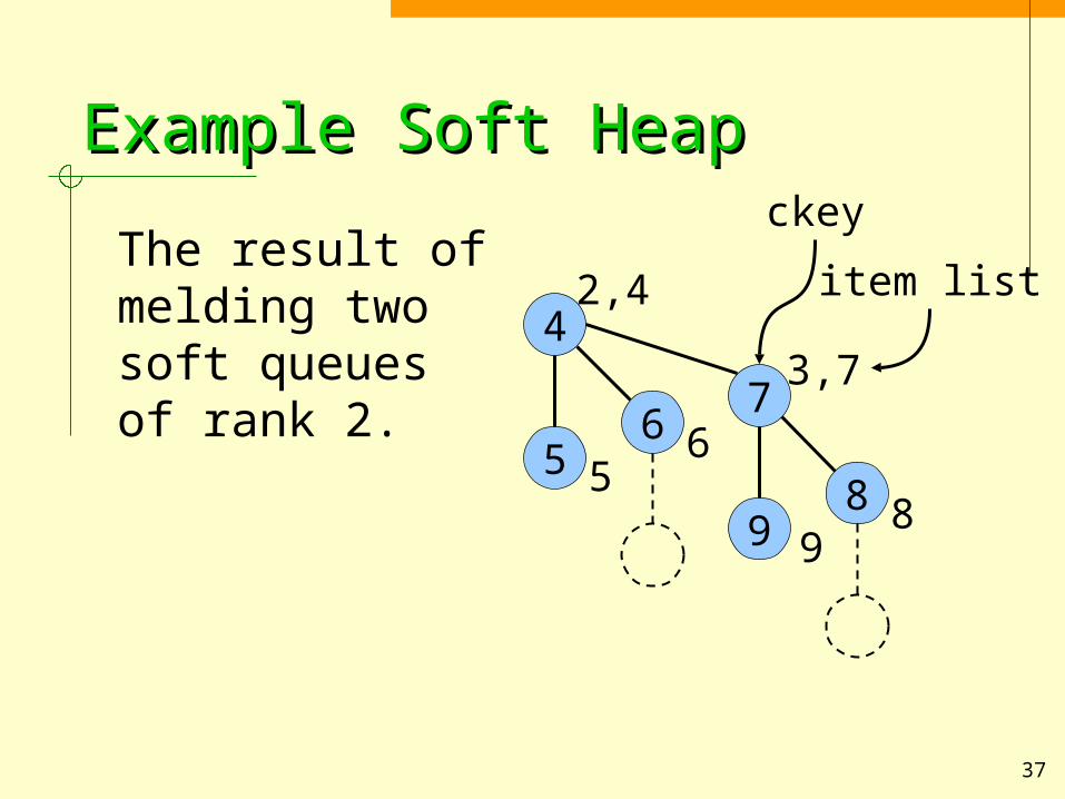
Example Soft HeapExample Soft Heap
The result of melding two soft queues of rank 2.
4
56
7
98
2,4
3,7
56
89
item list
ckey

38
SiftSift
sift(S)1. If S has one node, done.2. v = child of root with smallest
key3. Move key of v to root4. sift(sub-tree rooted at v)

39
Sift Sift SiftSift Sift Sift
sift(S)1. If S has one node, done.2. v = child of root with smallest
key3. Move key of v to root4. sift(sub-tree rooted at v)
5. If height of S is now odd, goto 1.

40
Final Word About Soft Final Word About Soft HeapsHeaps
Optimality

41
Minimum Spanning TreeMinimum Spanning Tree
Overview

42
Graph ModelGraph Model
G = (E,V)n verticesm edges,multiple edges allowed, but no self-loopsedge cost of e is c(e),WLOG assume all distinct

43
A Brief History of MSTA Brief History of MST1926 Boruvka O(m log n)1930 Jarnik ..1956 Kruskal ..1957 Prim ..1974 Tarjan (unpublished)O(m (log n)1/2)1975 Yao O(m log log n)1976 Cheriton and Tarjan O(m log logd n), d=max(2,
m/n)1986 Fredman and Tarjan O(m (m,n))1986 Gabow et al. O(m log (m,n))1990 Fredman and WillardO(m), RAM1994 Klein and Tarjan O(m), randomized1997 Chazelle O(m (m,n) log (m,n))1999 Chazelle, Pettie O(m (m,n))

44
Two RulesTwo Rules
CutThe cheapest edge crossing any cut is in the MST.
CycleThe costliest edge on any cycle is not in the MST.

45
Cycle RuleCycle Rule
CycleThe costliest edge on any cycle is not in the MST.
That also means if an edge is not in the MST, there must be a cycle that witnesses this fact.
(What is that cycle?)

46
The Sampling AdvantageThe Sampling Advantage
Most methods use divide-and-conquer by splitting up the graph using either
the distribution of the edge costs, or
the combinatorial structure,but rarely both.
Sampling allows us to do both at once.

47
Deterministic SamplingDeterministic Sampling
Find a low discrepancy subgraph whose own MST bears witness to the non-MST status of many edge.
(Still remember the cycle rule?)

48
Two NotationsTwo Notations
G*R The graph derived from G by raising the costs of all edges in R µ E.
G\C The graph derived from G by contracting the subgraph C into a single vertex c.

49
ContractionContraction
28
14 12
4 96
17
23
12
4 96
17
23
C
G\CG
50
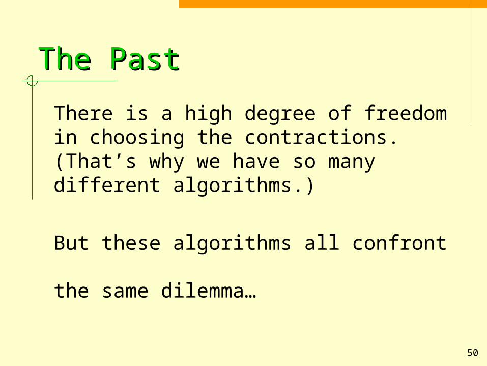
The PastThe Past
There is a high degree of freedom in choosing the contractions. (That’s why we have so many different algorithms.)
But these algorithms all confront the same dilemma…

51
DilemmaDilemma
Many MST algorithms identify the cheapest edge crossing a cut by maintaining all eligible edges in a heap.
But as the graph gets contracted, the degree of vertices tend to grow. So, finding the cheapest edge becomes more and more difficult.

52
Typical StrategyTypical Strategy
Keep a heap for each vertex.When contract, meld heaps and delete edges.
Degrees grow) Bigger heaps) Slower heaps!

53
Heap Design Matters!Heap Design Matters!
We would like deletion to be fast.
Higher in heap ) Slower to delete

54
SiftSift
sift(S)1. If S has one node, done.2. v = child of root with smallest
key3. Move key of v to root4. sift(sub-tree rooted at v)

55
Heap Design Matters!Heap Design Matters!
We would like deletion to be fast.
Higher in heap ) Slower to delete
So, if an edge is likely to be deleted, we want to store them low. But if their costs are low, how do we do that?

56
Soft HeapsSoft Heaps
Items with keys from a total order
create(S)delete(S, x)findmin(S)meld(S, S’)insert(S, x)
Amortized O(1)
O(log 1/)

57
Sift Sift SiftSift Sift Sift
sift(S)1. If S has one node, done.2. v = child of root with smallest
key3. Move key of v to root4. sift(sub-tree rooted at v)
5. If height of S is now odd, goto 1.

58
Key HidingKey Hiding
We can hide thesmall keys intothe item list…
4
56
7
98
2,4
3,7
56
89
item list
ckey

59
The PlanThe Plan
Many MST algorithms identify the minimum cost edge crossing a cut by maintaining all eligible edges in a heap. soft
Aren’t wedone now?Aren’t wedone now?

60
Our Affair With CorruptionOur Affair With Corruption
Unless all edges crossing a cutare not corrupted, the cheapest such edge is not guaranteed to be in MST(G).
The costliest edge in a cycle is not in MST(G) only if it is uncorrupted.

61
Cut vs. CycleCut vs. Cycle
Forget about the cut rule.Use the cycle rule instead.
But how can the cycle rule be applied efficiently?

62
Minimum Spanning TreeMinimum Spanning Tree
The Real Plan

63
Contractible SubgraphContractible Subgraph
A subgraph C is contractible if its intersection with the MST is connected.

64
Alternative DefinitionAlternative Definition
C is contractible if for any edges e and f, each having one endpoint in C, there exists a path connecting e to f in C consisting of edges with costs less than max(c(e), c(f)).

65
Lemma 1Lemma 1
If C is contractible w.r.t. G, then MST(G) = MST(C) [ MST(G\C).
Show ProofShow Proof

69
Why Contractibility is Good?Why Contractibility is Good?
A small but significant saving: when computing MST(C), avoided 3 edges.
28
14 12
4 96
17
23
12
4 96
17
23
C
G\CG

70
Lemma 2Lemma 2
If C is contractible w.r.t. G*R, and RC are those edges in R with one endpoint in C, then
MST(G) µ
MST(C) [ MST(G\C*RC) [ RC.
Show ProofShow Proof

75
How to find?How to find?
Typical algorithms find contractible subgraphs by computing their MSTs.
We use soft heaps.

76
The Real Plan - OverviewThe Real Plan - Overview
Relax the contraction rule (by means of cost corruption) and contract edges that are not really cheapest, but only nearly so.
We will have a spanning tree that is not minimum, but hopefully, nearly so.

77
In ParticularIn Particular
This almost-minimum spanning tree
will become our witness in rejecting many edges (using the cycle rule).
How do we turn this almost-minimum spanning tree into the real one? Use recursion
to bootstrap!Use recursionto bootstrap!

78
Stage 1Stage 1
Consider G0 = G*R. Partition G0 into contractible subgraphs and contract each into a vertex. Repeat. (G1, G2…)
When a subgraph is contracted, corrupted edges with one endpoint in that subgraph will be marked as bad.

79
Stage 2Stage 2
Recur on the non-bad edges of each contracted subgraph, return its MST.
(Non-bad edges will be restored to their original costs before recursion, i.e. we get the true MST of the subgraph.)

80
Stage 3Stage 3
Recur on the graph consisting of edges returned in stage 2 and the bad edges in stage 1 (with edge costs restored).
Repeatedly use Lemma 2 to conclude that this set of edges contains the MST of the original graph.

81
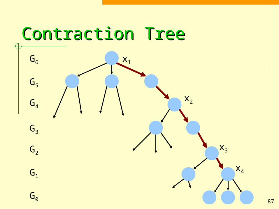
Minimum Spanning TreeMinimum Spanning Tree
ContractionTree

82
NodesNodes
A node x in T with height h represents both a vertex vx of Gh and a subgraph of Gh-1.
The children of x represents those vertices of Gh-1 contracted to form vx.

83
Contraction TreeContraction TreeG6
G5
G4
G3
G2
G1
G0

84
Building In Post-orderBuilding In Post-order
x is “under construction” if only some of x’s children are finished.
At any time, there will only be at most one subgraph from each of Gd, …, G0 that is under construction.(d is the height of T.)

85
Time To ContractionTime To Contraction
When the subgraph of Gi has reached a critical size (which depends on i),we contract the subgraph into a single vertex and add it to the subgraph of Gi+1, which is under construction.
(This may cause a upward propagation of contractions.)

86
Active SubgraphsActive Subgraphs
Let X be a sequence of subgraphs X1, …, Xk that are under construction and currently have at least one vertex.
Maintain the invariant that for all i, h(Xi) ¸ h(Xi+1).
87
Contraction TreeContraction TreeG6
G5
G4
G3
G2
G1
G0
x1
x2
x3
x4

88
External vs. InternalExternal vs. Internal
Edges with one endpoint in X are called external.
Edges with both endpoints in X are called internal.
Notice that an external edge can become internal later.
89
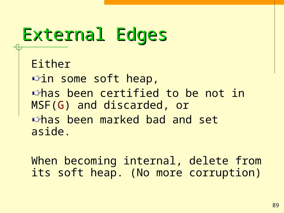
External EdgesExternal Edges
Eitherin some soft heap,has been certified to be not in
MSF(G) and discarded, orhas been marked bad and set
aside.
When becoming internal, delete from its soft heap. (No more corruption)

90
Cost Cost CostCost Cost Cost
Heap cost – cost in soft heap
Current cost – heap cost if external or bad, original cost otherwise
After T has been built (so no more external edges), the final cost is the current cost.

91
The Truths About CostThe Truths About Cost
Heap costs never decreases.
If an internal edge is not bad, then current = final = original.
The final cost of a bad edge will be no less than its current cost.

92
Current Cost InvariantCurrent Cost Invariant
Let g be the edge of minimum current cost between Xi and Xi+1. The current cost of g is cheaper than the current cost of (i) all external edges incident on Xj for j · i, and (ii)internal edges between distinct
Xj, Xk for j, k · i.

93
Current Cost of Current Cost of gg
… cheaper than the current cost of (i) all external edges incident on Xj for j · i
Easy. (We are building in post-order.)

94
Current Cost of Current Cost of gg
… is cheaper than the current cost of (ii)internal edges between distinct
Xj, Xk for j, k · i.
Maintain an edge min-link(j, k) between each Xj, Xk for j, k · i.

95
RetractionRetraction
Mark all corrupted external edges incident to Xk as bad.
Contract Xk into xk and add it to the subgraph of Gh-1. Generally, this will be Xk-1.
But if height of Xk-1 is higher than h+1, then create Xk = {xk} at height h+1.
Update min-links to preserve the Invariant.

96
ExtensionExtension
Select the cheapest (using current cost) external edge (u, v) with u 2 X. Add v to X.
Do retractions if some subgraphs now reach their critical sizes.
Maybe non-trivial to maintain the Invariant when v arrives. We break it down into cases.

97
Simple ExtensionSimple Extension
If u 2 Xk and for all i, j, current-cost(u, v) < min-link(i, j), then
Create Xk+1 at height 0.
Let Xk+1 = {v}.
Find min-link(i, k+1) for all i · k.k++
Else do Complex Extension

98
Invariant PreservationInvariant Preservation
(u, v) is the cheapest external edge
current-cost(u, v) < min-link(i, j)
When (u, v) is added to X,its current cost may only drop (when it is corrupted but not bad).
Current costheap cost if
external or bad,original cost
otherwise.
Current costheap cost if
external or bad,original cost
otherwise.

99
Complex ExtensionComplex Extension
Find minimum i s.t. for some j,min-link(i, j) < current-cost(u, v).Perform retractions until Xi+1 is the last subgraph in X. Then contract Xi+1 into z.
Perform a fusion:Let (w, z) be min-link(i, i+1) for w 2 Xi.
Contract (w, z), the fusion edge.Now can do simple extension on (u, v).

100
Invariant PreservationInvariant Preservation
minimum i s.t. for some j,current-cost(u, v) > min-link(i, j)
Retractions to eliminate such min-links
We have just contracted subgraphs Xi+1, Xi+2, …, Xk into z.

101
Complex Extension PictureComplex Extension Picture
Current costs indicated by height on slide.
Min-links cheaper than (u, v) are dotted.
Xi-1 Xi Xi+1 Xk
u
v
w

102
FusionFusion
(w, z) is min-link(i, i+1) for w 2 Xi.
We claim that (w, z) is contractible w.r.t. final cost. (Lemma 4, later)
Call the resulting dummy vertex fuse(w, z).

103
Just Before FusionJust Before Fusion
(u, v) is the cheapest external edge and (w, z) is the only min-link cheaper than (u, v).
Xi-1 Xi Xi+1
(u,v)v
w z

104
Just After FusionJust After Fusion
(w, z) has been contracted. The number of vertices in Xi doesn’t change.
Xi-1 Xi Xi+1
fuse(w,z) v

105
Fusion PictureFusion Picture
w z
xi
w z
xi
fuse(w,z)

106
Contraction TreeContraction Tree
Lemmas

107
Lemma 3Lemma 3
At all times and for all i,Xi is contractible w.r.t. current costs.
Current costheap cost if
external or bad,original cost
otherwise.
Current costheap cost if
external or bad,original cost
otherwise.
Show ProofShow Proof

112
Lemma 4Lemma 4
Let C be a subgraph or fusion edge contracted while building T, then C is contractible w.r.t. final costs.
Final costEquals to currentcost after Thas been built.
Final costEquals to currentcost after Thas been built.
Show ProofShow Proof

116
Lemma 5Lemma 5
Let G*B be the graph under final costs, where B is the set of bad edges.Let x be some node in T and Cx be the corresponding subgraph.
Then MST(G) µ [x2T MST(Cx\B) [ B.
Show ProofShow Proof

120
Contraction TreeContraction Tree
Construction

121
nnamrekcA FunctionnnamrekcA Function
j ¸ 1: A(1, j) = 2j
i > 1: A(i, 1) = A(i-1, 2)o.w.: A(i, j) = A(i-1, A(i, j-1))
(m, n) = min { i | A(i, dm/ne) > log n}

122
ParametersParameters
Pickd = d(m/n)1/4et = min { t’ | A(t’, d) ¸ n }
We will later show that t · (m, n) + 2.

123
Critical SizeCritical Size
If Xi has height hi, then its critical size is A(t, hi).
If hi is 0, then critical size is 1.
124
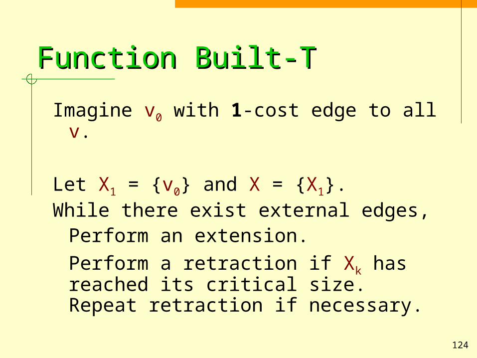
Function Built-TFunction Built-T
Imagine v0 with 1-cost edge to all v.
Let X1 = {v0} and X = {X1}.While there exist external edges,
Perform an extension.Perform a retraction if Xk has reached its critical size. Repeat retraction if necessary.

125
Lemma 6Lemma 6
The number of vertices in a multi-vertex subgraph of Gi contracted while building T is no more than 2n/A(t, i).
Show ProofShow Proof

131
Minimum Spanning TreeMinimum Spanning Tree
MSTAlgorithm

132
DensityDensity
Assume G has density m/n ¸ c(m,n) for a large enough c.

133
Lemma 7Lemma 7
The density of G can be increased to D by contraction in O(m + n log D) time.
Proof:Perform one pass of Fredman-Tarjan.

134
Function MSFFunction MSF
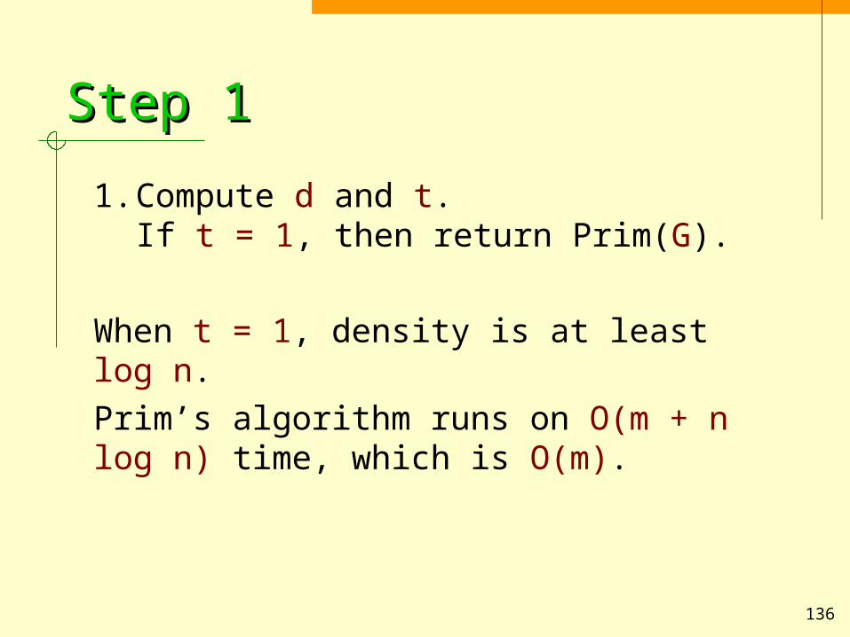
1. Compute d and t.If t = 1, then return Prim(G).
2. T = Build-T()Let B be the set of bad edges.
3. For all x2T, let Cx be the corresponding subgraph except the bad edges.Improve density of Cx to get C’x.Store contracted edges in Fx.

135
Function MST - ContinuedFunction MST - Continued
4. Let G’ be [x2T (MSF(C’x) [ Fx) [ B.
5. Improve density of G’ to get G’’. Store contracted edges in F’.
6. Return MSF(G’’) [ F’.
136
Step 1Step 1
1. Compute d and t.If t = 1, then return Prim(G).
When t = 1, density is at least log n.Prim’s algorithm runs on O(m + n log n) time, which is O(m).

137
Step 2Step 2
2. T = Build-T()Let B be the set of bad edges.
Just recall that bad edges are corrupted incident edges when contracting a subgraph. Here their costs has been restored.
We will take care of them in steps 4 and 6.

138
Step 3Step 3
3. For all x2T, let Cx be the corresponding
subgraph except the bad edges.Improve density of Cx to get C’x.
Store contracted edges in Fx.
All edges stored in Fx are MST edges.
Density improvement needed to make sure t decreases in the next step.

139
Step 4Step 4
4. Let G’ be [x2T (MSF(C’x) [ Fx) [ B.
We compute the MST of C’x (which does not have bad edges).Union that with Fx gives the MST of Cx.
Then we throw in the bad edges, preparing for the next recursion.

140
Step 5Step 5
5. Improve density of G’ to get G’’.Store contracted edges in F’.
Again, edges stored in F’ are in the MST.
Density improvement needed to make sure t does not increase in the next step.
141
Step 6Step 6
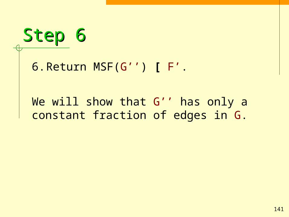
6. Return MSF(G’’) [ F’.
We will show that G’’ has only a constant fraction of edges in G.

142
Density BusinessDensity Business
Why we need to improve the density in steps 3 and 5 (except that we want the math to work out)?
Sadly, part of the trick when doing double recursion is to get the math to work out…

143
Executive SummaryExecutive Summary
You only need to know
They take time linear to the number of edges of the input graph.
They are “doable”, albeit quite complicated.
144
Minimum Spanning TreeMinimum Spanning Tree
Running Time

145
Lemma 8Lemma 8
Built-T runs in time O(m log 1/ + d2n) and generates O( m + d3n) bad edges, for any < ½.
We will prove this later.

146
Lemma 9Lemma 9
Our choice of t implies t = O((m, n)).
Recall:(m, n) = min { i | A(i, dm/ne) > log n}d = d(m/n)1/4et = min { t’ | A(t’, d) ¸ n }
Show ProofShow Proof

150
Theorem Of The DayTheorem Of The Day
The MSF of a graph with m edges and n vertices can be computed in (deterministic) O(m(m, n)) time.
Proof sketch:Write a recurrence and do induction to conclude T(m, t) · c1tm.

154
Minimum Spanning TreeMinimum Spanning Tree
HeapManagement

155
What?What?
Naïve heap management will lead to O(m log n) solution.
Show DetailsShow Details

161
The Discrepancy MethodThe Discrepancy Method
Ending Words

162
Latest DevelopmentLatest Development
Seth PettieAn Inverse-Ackermann Style Lower Bound for the Online Minimum Spanning Tree Verification Problem
(FOCS 2002)

163
Open QuestionsOpen Questions
What is the complexity of MST?
Non-“data-structure approach” to MST?
Simple, practical algorithm for MST verification?

164
MoralMoral
Finding a suitable low discrepancy subset is hard.
Perhaps this shines some light onhow useful random bits really are(in terms of efficiency)?
165
FinallyFinally
It’s OK to forget the theorems and the proofs,
but not the method.
166
Low Discrepancy Sub-TalkLow Discrepancy Sub-Talk
In fact, if you forget the proofs, what you will have is precisely a low discrepancy sub-talk. :P
(i.e. the benefit of understanding the sub-talk is “close to” that of understanding the whole talk)

194
The EndThe End
Like the lemon bar?