Bayesian Networks

Matthew Pettigrew

Department of Mathematical Sciences

Montana State University

May 5, 2016

A writing project submitted in partial fulfillmentof the requirements for the degree

Master of Science in Statistics

APPROVAL

of a writing project submitted by

Matthew Pettigrew

This writing project has been read by the writing project adviser and has been foundto be satisfactory regarding content, English usage, format, citations, bibliographicstyle, and consistency, and is ready for submission to the Statistics Faculty.

Date John BorkowskiWriting Project Adviser

Date Mark GreenwoodWriting Projects Coordinator

BN 1

1 Introduction

With the advent of computers and big data, cutting edge statistical modeling andmethods are developing to take advantage of the additional computational power,dive into the abundance of information, and answer questions about our world frommore complex perspectives while potentially accounting for more latent informationand dependencies. While these new methods and technology have challenged ourepistemological ideas of causality, objectivity, and evidence, such philosophicalarguments are not the focus of this paper. Instead, this paper will explore oneupcoming method, Bayesian Networking, and it’s use. I will explore it’s generalunderlying theoretical framework while providing the reader with a clear picture ofhow a Bayesian network works.

1.1 What is a Bayesian Network

“A Bayesian network is a graphical structure that allows us to represent and reasonabout an uncertain domain. The nodes in a Bayesian network represent a set ofrandom variables from the domain. A set of directed arcs connect pairs of nodes,representing the direct dependencies between variables.” (Korb & Nicholson, 2011)

The definition provided by Korb and Nicholson captures the essence of BayesianNetworks. A Bayesian Network is a statistical modeling technique utilizing a graphicalstructure comprised of nodes and directed arcs to visualize the model. Each node ofthe graph represents a random variable from our data or created from our data.Each random variable is composed of a set of observations corresponding to casesfrom the original data set. Dependencies between random variables are directlyrepresented by directed arcs, arrows, that indicate the direction of the dependency.Each random variable can be directly dependent on multiple random variables or havemultiple random variables be dependent on it. The variables that a random variableis dependent on are its parents, while variables that are dependent on a given randomvariable are its children.

In contrast, the general linear modeling framework requires one variable, theresponse, to be dependent on a set of explanatory variables. While in certainsituations the application of linear modeling is quite adequate, the modelingstructure of Bayesian networks allows for more flexibility by accounting for multipledependencies. There can be multiple response variables that share some or no parentpredictors. A given random variable can be both a response and an explanatoryvariable within the same model. Bayesian Networking allows for modeling and testingthe inherent dependencies within the network.

A Bayesian network utilizes the full joint probability distribution of a set ofrandom variables and conditional factorization exploiting the direct dependenciesand the Markov Property. This means that the full joint probability distributionis factored into a set of conditionally independent local distributions. Each localdistribution consists of the probability distribution of a random variable conditionalon its parents. This factorization allows for localization of calculations. Additionally,the localization allows for the model to incorporate information from cases with

BN 2

missing data and make predictions, referred to as belief updating, with partial data.

1.2 Graphical and Probabilistic Representation

The graphical and probabilistic representation of a Bayesian network are possible dueto the Markov Property, which allows the graphical model to be seamlessly mappedto the conditional factorization of the full joint distribution. Korb and Nicholsondescribe the Markov property as such: “there are no direct dependencies in the systembegin modeled which are not already explicitly shown via arcs” (Korb & Nicholson,2011). In essence this states that the probabilistic representation of the model shouldreflect the dependencies of the graphical representation via the arcs. Scutari and Denis(2014) also provide a formal definition in terms of conditional independencies: “Eachnode Xi is conditionally independent of its non-descendants (e.g. nodes Xj for whichthere is no path from Xi to Xj) given its parents”. Likewise, this definition statesthat the probabilistic representation should reflect the conditional independencies ofthe graphical representation. If either condition is violated then the Markov Propertyis not met.

The Markov property is best illustrated by example. Figure 1 represents anexample of a generic Bayesian Network comprised of the random variables ’A’ through’F’ that could be modeled by their joint probability distribution P (A,B,C,D,E, F ).The joint distribution is conditionally factored so that each variable is conditionallydependent on its parents. The root nodes, A and B, have no parents and arerepresented as their respective marginal distributions P(A) and P(B). Node C has twoparents, A and B, and thus its probabilistic conditional factorization is P (C|A,B).Node E has one parent, C, and its conditional probability distribution is P (E|C).However, Node E is also dependent on A and B as there is a directed path fromA to E and likewise from B to E. These directed paths pass through C, E’s onlydirect dependency. Thus, Node E is dependent on A and B only through C. Afterconditioning E on C, A and B no longer provide information to E. This is the MarkovProperty in action. Conditioning D on C results in a similar scenario to conditioningE on C. Finally, conditioning F on D and E will result in F being conditionallyindependent from C, B, and A, which will no longer be able to pass information toF.

BN 3

A B

C

D E

FFigure 1: P (A,B,C,D,E, F ) = P (A)P (B)P (C|A,B)P (D|C)P (E|C)P (F |D,E)

1.3 ALARM Example

Let’s examine a quick motivating example to find out what a Bayesian Network cando. The ALARM monitoring system is a Bayesian Network created by Beinlich,Suermondt, Chavez & Cooper (1989), that“is often used as a benchmark in the BNliterature” (Korb & Nicholson, 2011).“The goal of the ALARM monitoring systemis to provide specific text messages advising the user of possible problems” and ”is adata-driven system. Simulating an anesthesia monitor.”

The system consists of three types of variables denoted diagnoses, measurements,and intermediate variables. The measurements are physiological measurements, suchas heart rate and blood pressure, measured from a patient currently undergoingsurgery. The intermediate variables are variables that cannot be directly observedbut can be easily calculated from the physiological measurements, such as the ratioof HR/BP. The diagnoses are diseases or potential issues with the patient receivingthe proper amount of anesthesia. The entire network, shown below, consists of47 variables (8 diagnoses and 16 measurements). The Bayesian network uses thedata from the physiological measurements and estimates the probability of eachdiagnosis given the conditional distribution estimated from the data. If the estimatedprobability of a diagnosis crosses an upper threshold, the system triggers an ALARMalerting the anesthesiologist of the problem and the possible causes along with theassociated probabilities. The anesthesiologist can then take action and remedy the

BN 4

situation before harm is inflicted on the patient.

HISTORY

CVPPCWP

HYPOVOLEMIA

LVEDVOLUME

LVFAILURE

STROKEVOLUME ERRLOWOUTPUT

HRBP HREKG

ERRCAUTER

HRSAT

INSUFFANESTH

ANAPHYLAXIS

TPR EXPCO2

KINKEDTUBE

MINVOLFIO2

PVSAT

SAO2

PAP

PULMEMBOLUS

SHUNT

INTUBATION

PRESS

DISCONNECT

MINVOLSET

VENTMACH

VENTTUBE

VENTLUNG

VENTALV

ARTCO2

CATECHOL

HR

CO

BP

Figure 2: The ALARM Bayesian Network (Beinlich, 1989)(Scutari, 2015)

2 Graph Theory

Before looking more deeply into Bayesian networks, we need to look at the basicunderlying graph theory. The graphical representation of the model is a key visual

BN 5

tool to understand how assumptions, estimates, and calculations filter through thenetwork. The introduction provided two key ideas: nodes and directed arcs. Nodesrepresent random variables, while directed arcs, which connect two nodes, modeldirect dependencies. A directed arc connects a parent to a child. Undirected arcs canalso connect two nodes and are illustrated as a line segment between the two nodes.Certain algorithms utilize undirected arcs or represent uncertainty in the direction ofa dependency by not directing an arc. Bayesian networks, however, must consist ofonly directed arcs.

2.1 Directed Acyclic Graphs

The graphical structure of a Bayesian network must be a Directed Acyclic Graph(DAG). A DAG consists of nodes connected only using directed arcs. Additionally thegraph must be acyclic, that is, the graph cannot contain any loops. A graphical loopwould indicate a cycle of dependencies among a subset of variables in the model (seeFigure 3(b)). More specifically, the conditional factorization of the joint distributionwould no longer be valid for the inherent conditional probabilities. If including adependency which creates a cycle is necessary, another modeling technique should beused. Including the arc violates our conditional factorization, while not including thearc would violate our Markov Property. As such the underlying graphical structureof Bayesian Networks are strictly limited to DAGs.

(a) Acyclic

Ancestor

A

Descendent

(b) Cyclic

Ancestor

A

Descendent

X

Figure 3: (a): A simple DAG as all directed paths go from ancestor to descendent.(b): Adding a directed arc from the descendant to the ancestor creates a cycle. Thegraph is no longer a DAG.

2.2 Connections

Three nodes can be fundamentally connected in three ways which result in a DAG.These fundamental connections represent the possible direct dependencies that canbe modeled and provide the basic framework for how the Markov Property operatesbetween a subset of nodes within the graph. The serial connection consists of three

BN 6

nodes in a straight line with a central node that has both a parent and a child (Figure4(a)). The divergent connection consists of single parent with two children (Figure4(b)). Lastly, the convergent connection consists of child node having two parents. Aspecial type of convergent connection known as a V-structure occurs, when the twoparents are not connected by an arc (Figure 4(c)).

(a) Serial Connection

A

B

C

(b) Divergent Connection

A

B C

(c) V−Structure

A B

C

Figure 4: The three types of DAG connections.

By conditioning on B, the central node in the serial connection, the nodes Aand C are effectively cutoff from one another (Figure 5(a)). Nodes A and C aregraphically separated, or graphically independent, after conditioning on B. By theMarkov Property this implies that A and C are probabilistically independent afterconditioning on B. As such, nodes A and C are D-separated (from direction-dependentseparation) (Korb & Nicholson, 2011).

Similarly, by conditioning on the parent node, A, of the divergent connection,the same results occurs (Figure 5(b)). In the divergent case after conditioning onA, the nodes B and C are D-separated; that is B and C are both graphically andprobabilistically independent after conditioning on A.

The V-structure exhibits a quite different relationship. The parents nodes, Aand B, are graphically and probabilistically independent without conditioning on C(Figure 4(c)). A and B are D-separated. However, after conditioning on C commoninformation would be pass to A and B via Bayes Theorem. As such, conditioningon C creates a relationship between A and B (Figure 5(c)). Given C, A and Bare no longer graphically or probabilistically independent. This does not, however,violate the Markov property as the direction the information flows does not affect theconditional factorization of the model.

(a) Serial Connection

A B C

(b) Divergent Connection

A

B C

(c) V−Structure

A B

C

Figure 5: The three types of DAG connections after conditioning on the central node.

BN 7

2.3 Markov Blankets

The three types of basic DAG connections, D-separation, and the Markov propertyprovide the basis for the next important idea from Graph Theory for Bayesiannetworks, the Markov Blanket. A Markov Blanket of a node consists of the node’sparents, children, and the other parents of its children. The Markov Blanket of nodeD from our original generic Bayesian network is highlighted in figure 6. Node D’sonly parent is node C, its only child is node F, and lastly, node E is also a parent ofF and is thus part of node D’s Markov Blanket.

A B

C

D E

F

Figure 6: The Markov Blanket for node D consists of nodes C, E, and F.

The Markov Blanket of a node is the core idea for updating our beliefs aboutthe local distribution of a particular node. First, recall that our local distributionfor node D was P(D|C) as specified by the conditional factorization and the MarkovProperty. However, any evidence obtained for node F, D’s only child, could directlyupdate our beliefs about node D via Bayes’ Theorem. Furthermore, conditioning onnode F creates a direct dependency between D and E due to the V-structure. Thus,conditioning on E is necessary to account for all of D’s potential dependencies. Hence,a Markov Blanket of a node consists of the set of nodes that could potentially affectour beliefs about D directly. Moreover, the Markov Blanket is the set of nodes whichD-separates a node from the rest of the network.

In turn, Markov Blankets allow for the localization of calculations when beliefupdating. In contrast, we could condition a node on every other node in the networkto update our beliefs. “However, this is unfeasible for most real-world problems, and

BN 8

in fact it would not be much different from using the global (full-joint) distribution”(Scutari & Denis, 2104). In other words, conditioning on every other node in thenetwork would create a great deal of computational complexity while contendingwith the ’curse of dimensionality’. The Markov Blanket allows the computationalaspect of belief updating to circumvent the curse and focus only on the necessaryinformation needed for inference about a particular node.

3 Bayesian Networks

The preceding section on Graph Theory was not a comprehensive overview of thegraphical ideas present in Bayesian networking, but only a quick survey of thefundamental ideas necessary to get a clear picture of the inner workings of themodeling technique. With these ideas in place, we now have the tools to examinehow local distributions are specified, how the dependencies are specified or learned,and how, via the dependencies, local distributions are updated. The probabilisticestimations rely on extensions of basic probability theory and Bayesian statistics(although frequentist methods are available) and are carried out utilizing complexalgorithmic techniques developed in Computer Science.

Many of the developed methods for handling Bayesian networks are available in avariety of software packages like BayesiaLab, Hugin, Netica, and GeNIe to namea few. R alone boasts several packages such as bnlearn, catnet, deal, gRbase,and gRain. Due to extensive techniques, types of models, and algorithms availablefor estimation, learning, and updating, much of the available software specializes inparticular applications. The focus of the rest of the paper will be on Discrete BayesianNetworks, which utilize only discrete (categorical) random variables.

Bayesian networks are not limited to discrete random variables. There aremethods available for networks made entirely of continuous variables (GaussianBayesian networks), networks consisting of discrete and continuous variables (HybridBayesian networks), networks with serially correlated data (Dynamic Bayesiannetworks), and applications augmented with decision and utility nodes (DecisionGraphs). However, discrete Bayesian networks provide a simplistic environment; eachlocal distribution is specified by a conditional probability table, and calculations arelimited to conditional and marginal probabilities contained in the cells of the table.Furthermore, most of the available Bayesian networking software can handle discretenetworks, which is not the case for more complex Bayesian networking structuresmentioned above.

The methods illustrated in this paper utilize the bnlearn (Scutari, 2010) andgRain (Hojsgaard, 2012) packages from R with additional graphical support fromthe Rgraphviz (Hansen et al.) package.

3.1 Parameter Learning

The local distributions for a discrete Bayesian network are conditional probabilitytables where each node is assumed to follow a multinomial distribution. The

BN 9

categorical probabilities of a variable are broken down conditionally on eachcategorical combination of the its parents’ categorical levels. For a motivatingexample, the Cancer network presented by Korb and Nicholson, (2011) is used andis available in the (bnlearn) package (Scutari, 2010). This small network consistsof 5 two-level categorical variables and is designed to estimate the probability oflung cancer given two contributors to lung cancer (pollution and smoker) and twosymptoms (X-ray and Dyspnoea).

Pollution Smoker

Cancer

Xray Dyspnoea

Figure 7: The Cancer BN from Korb and Nicholson, 2001

As the root nodes Pollution and Smoker do not have parents, their localdistributions (Table 1) are simply the estimated marginal distributions. Theestimated probability for exposure to low level pollution is 0.9, while high levelpollution is 0.1. The estimated probability of a patient being a smoker is 0.3.

Pollution

low 0.90high 0.10

Smoker

True 0.30False 0.70

Table 1: Marginal Distributions of Pollution and Smoker

Cancer, however, has two parent nodes, and its local distribution is representedby a three dimensional conditional probability table (Table 2). Patients exposed tolow levels of pollution that are also smokers have an estimated probability of 0.03of having lung cancer and 0.97 of not having lung cancer. Changing exposure topollution to high increases the estimated probability of having cancer to 0.05.

The local distributions for X-ray and Dyspnoea are represented by a typicaltwo-dimensional probability table as each node has a single parent, cancer (Table 3).Examining the Dyspnoea table reveals that patients which have lung cancer have anestimated probability of 0.65 to be suffering from shortness of breath, while patientswhich do not have lung cancer have an estimated probability of 0.30.

BN 10

Pollution: low high

Cancer Smoker: True False True False

True 0.030 0.001 0.050 0.020False 0.970 0.999 0.950 0.980

Table 2: Conditional Distribution of Cancer given Pollution and Smoker

Cancer

Xray True False

positive 0.90 0.20negative 0.10 0.80

Cancer

Dyspnoea True False

True 0.65 0.30False 0.35 0.70

Table 3: Conditional Distributions of X-Ray and Dyspnoea given Cancer

In practice the estimated probabilities and errors can be ’learned’ from the databy the respective Bayesian networking software. One common method for estimatingthe conditional probabilities is to simply use the appropriate MLEs (or proportions).Assuming the estimated probabilities in the above table are MLEs, then given allthe patients in the data set that have lung cancer, 65% of them are suffering fromDyspnoea. Whereas, of all the patients in the data set that smoke and have onlybeen exposed to low levels of pollution, 3% have lung cancer.

Another common estimation technique is to use a Bayesian posterior. In thiscase the MLEs are updated using a vague uniform prior with an imaginary samplesize (ISS) which determines the weight of the prior. Furthermore, many availablesoftware packages will allow user specification of the distributions including bothestimates and errors. As such, any Bayesian posterior can be input into the network,as well as estimates from bias corrected or variance inflated methods.

Another key advantage of Bayesian networks is their inherent ability to dealwith missing data. Parameter estimates can be calculated using the complete casesfor each local distribution. Then, if an observation has missing data, such as Smokerand Pollution but has data for the remaining three variables, then the distributionsfor X-ray and Dyspnoea can incorporate the available information from the partialobservation. The distributions for cancer, pollution, and smoker, however, will notincorporate the observation unless imputation methods are used.

3.1.1 Conditional Independence Tests

With local distributions estimated, we can assess the strength of the major modelassumption, i.e. conditional independence of the local distributions. This is done bytesting whether each of the included arcs (dependencies) should be in the networktypically by a log-likelihood ratio or Pearson’s X2 test for conditional independence.The null hypothesis for the test is that two nodes A and B are probabilisticallyindependent given a set of nodes C, while the alternative is that the respective nodes

BN 11

are not independent. That is,H0 : A ⊥⊥ B|C

HA : A 6⊥⊥ B|C

“Both tests have an asymptotic χ2 distribution under the null hypothesis” (Scutari& Denis, 2014), and large test statistics (small p-values) provide evidence that thetested arc should be in the network.

3.1.2 Network Scores

Two common scoring techniques are used to test the strength of the network asa whole, the Bayesian Information Criterion (BIC) and the Bayesian Dirichletequivalent uniform (BDeu or BDe). Both scores can be repeatedly calculated fordifferent networks created from the same set of variables. By removing and addingarcs and variables to a network a new score can be calculated and compared tothe score of the previous version of the network. For both tests a higher score isinterpreted to indicate a better model. As such, if adding an arc increases the score,then there is evidence supporting its inclusion in the network.

3.2 Structure Learning

Network scores and conditional testing provide the necessary tools to create thestructure of a Bayesian network. The structure of the network is the general layoutof the arcs and how they connect two different nodes. One method for creating thestructure of the Bayesian Network is completely apriori, using prior knowledge anddeductive reasoning about the variables. “In other words, we rely on prior knowledgeon the phenomenon we are modelling to decide which arcs are present in the graph andwhich are not” (Scutari & Denis, 2014). An important aspect of Bayesian networksand the Markov Property is to directly model the inherent direct dependencies ofthe variables. “The structure, or topology, of the network should capture qualitativerelationships between variables. In particular, two nodes should be connected directlyif one affects or causes the other, with the arc indicating the direction of the effect”(Korb & Nicholson, 2011). Often, to accomplish this task, the network is completelyuser specified, which tends to be more practical with fewer nodes.

The cancer example above provides a key illustration of this idea. Exposure tohigh levels of pollution and smoking both impact or cause a person to develop lungcancer. Once an individual has cancer, the chances of an x-ray having a positiveresult increases, as does the individual’s chance to suffer from shortness of breath. Assuch, the network is easily specified by deductive reasoning and prior knowledge.

Often, however, the necessary prior knowledge concerning the relationships of thevariables is not available. Generally speaking, it may be impractical to specify all therelationships, particularly with larger numbers of variables. The number of possiblenetworks grows “super-exponentially” with respect to the number of nodes. As such,learning the network algorithmically may be more practical (Scutari & Denis, 2014).

BN 12

3.2.1 Algorithms

A large amount of research has been specifically devoted to developing algorithms tolearn the structure of a Bayesian network. These algorithms are typically broken intothree types: constraint-based, score-based, and hybrid.

Constraint-based Constraint-based algorithms work by first learning the MarkovBlanket (or parents and/or children) of each node, which establishes undirected arcs.In turn, the algorithm is constrained by the Markov Blanket. This is done using one ofthe conditional independence tests from above with Monte Carlo versions of the testsavailable in many Bayesian networking software packages. Once the Markov Blanketfor nodes are established, the conditional independence tests can begin to determinethe directions of the arcs. Typically, the conditional independence tests will notdiscover all the dependencies. Many of the remaining undirected arcs, however, canbe directed to preserve the DAG by not inducing cycles. Different algorithms willthen handle the remaining undirected arcs differently. Some may set the directions toavoid inducing V-structures, while others will leave the arcs undirected and requirethe user to specify the remaining dependencies.

The constraint-based algorithms are based on Pearl’s Inductive Causation (IC)algorithm. The IC algorithm requires that every pair of nodes be checked forconditional independence, which in most instances is practically unfeasible. As suchthe exact IC algorithm has never been implemented but instead adapted by theMarkov Blanket constraint. The PC algorithm was the first implementable versionof Pearl’s IC. Other common constraint-based approaches include the Grow-ShrinkMarkov blanket (GS) algorithm and the Incremental Association Markov blanket(IAMB) algorithm. (Scutari & Denis, 2014)

Score-based Score-based algorithms attempt to maximize the BIC or BDe to findthe ”best” model. Greedy Search algorithms work be adding, dropping, and changingthe direction of arcs and keeping the changes which results in the largest score. Greedysearch algorithms most closely resemble the ’black-box’ techniques for finding the bestlinear model from a set of predictors. A common greedy search algorithm used inpractice in the hill-climbing algorithm. Other score-based techniques include geneticalgorithms and simulated annealing. Genetic algorithms explore various structuresthen combine their characteristics or randomly altering their structure in attemptto maximize the score. Simulated annealing algorithms tend to work similarly tothe greedy search algorithms but will accept changes that decrease the score with aprobability inversely proportional to the score decrease. (Scutari & Denis, 2014)

Hybrid Hybrid algorithms combine aspects from the constraint-based and score-based algorithms. Hybrid algorithms typically constrain each node by a set(s) ofcandidates of parents and/or children using conditional testing. Then, within thesecandidate sets, attempt to maximize the score using the score-based techniques fromabove. Commonly used algorithms include the Sparse Candidate (SC) algorithm and

BN 13

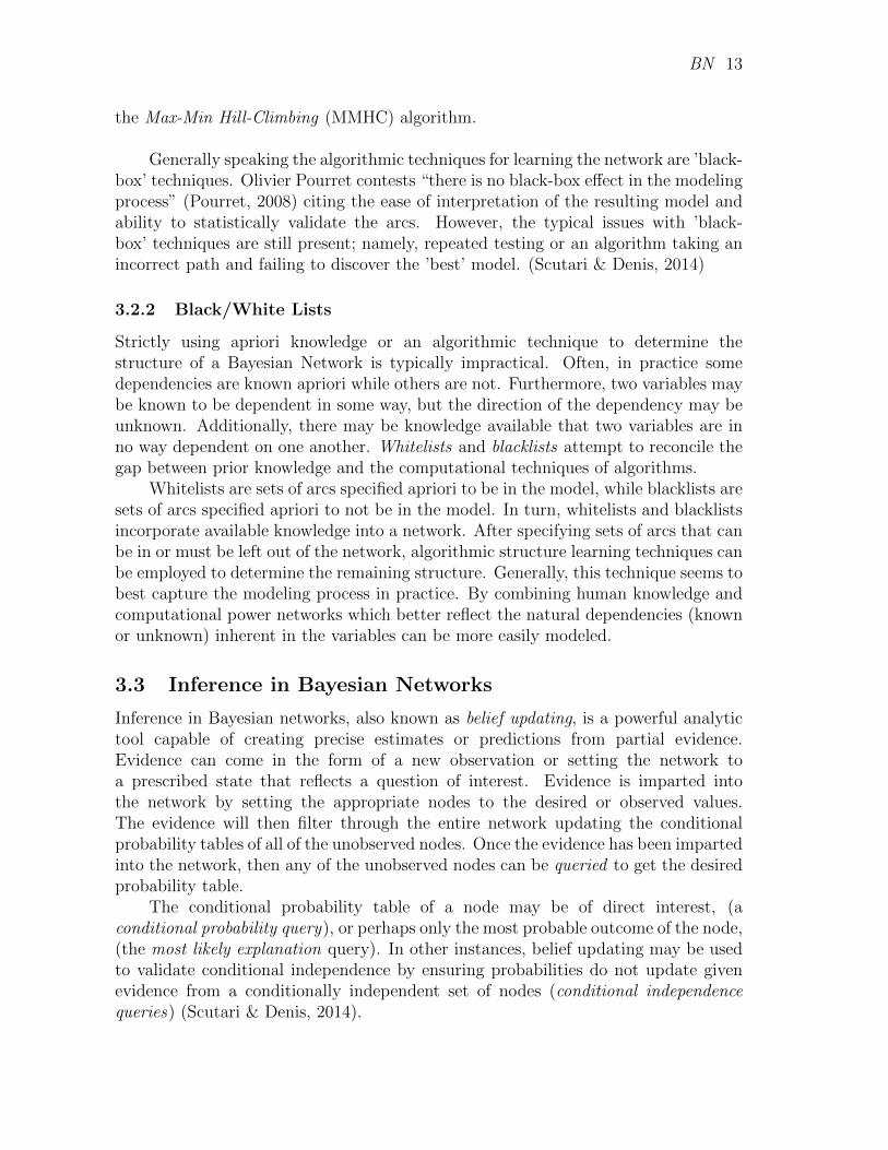
the Max-Min Hill-Climbing (MMHC) algorithm.

Generally speaking the algorithmic techniques for learning the network are ’black-box’ techniques. Olivier Pourret contests “there is no black-box effect in the modelingprocess” (Pourret, 2008) citing the ease of interpretation of the resulting model andability to statistically validate the arcs. However, the typical issues with ’black-box’ techniques are still present; namely, repeated testing or an algorithm taking anincorrect path and failing to discover the ’best’ model. (Scutari & Denis, 2014)

3.2.2 Black/White Lists

Strictly using apriori knowledge or an algorithmic technique to determine thestructure of a Bayesian Network is typically impractical. Often, in practice somedependencies are known apriori while others are not. Furthermore, two variables maybe known to be dependent in some way, but the direction of the dependency may beunknown. Additionally, there may be knowledge available that two variables are inno way dependent on one another. Whitelists and blacklists attempt to reconcile thegap between prior knowledge and the computational techniques of algorithms.

Whitelists are sets of arcs specified apriori to be in the model, while blacklists aresets of arcs specified apriori to not be in the model. In turn, whitelists and blacklistsincorporate available knowledge into a network. After specifying sets of arcs that canbe in or must be left out of the network, algorithmic structure learning techniques canbe employed to determine the remaining structure. Generally, this technique seems tobest capture the modeling process in practice. By combining human knowledge andcomputational power networks which better reflect the natural dependencies (knownor unknown) inherent in the variables can be more easily modeled.

3.3 Inference in Bayesian Networks

Inference in Bayesian networks, also known as belief updating, is a powerful analytictool capable of creating precise estimates or predictions from partial evidence.Evidence can come in the form of a new observation or setting the network toa prescribed state that reflects a question of interest. Evidence is imparted intothe network by setting the appropriate nodes to the desired or observed values.The evidence will then filter through the entire network updating the conditionalprobability tables of all of the unobserved nodes. Once the evidence has been impartedinto the network, then any of the unobserved nodes can be queried to get the desiredprobability table.

The conditional probability table of a node may be of direct interest, (aconditional probability query), or perhaps only the most probable outcome of the node,(the most likely explanation query). In other instances, belief updating may be usedto validate conditional independence by ensuring probabilities do not update givenevidence from a conditionally independent set of nodes (conditional independencequeries) (Scutari & Denis, 2014).

BN 14

Imparting evidence into leaf nodes with the desire to obtain information from itsparents or ancestors is known as diagnostic reasoning. Diagnostic reasoning movesagainst the direction of the arcs. A doctor may try to diagnose lung cancer fromsymptoms like Dyspnoea. Predictive reasoning occurs when moving in the directionof the arcs. Evidence is entered into root nodes with the desire to query from itschildren or descendants. A doctor may try to predict whether a person has or will getlung cancer given they are a smoker. Intercausal reasoning garners information about“mutual causes of a common effect” which has extended applications with respect toV-structures. In many instance predictive and diagnostic reasoning are combined. Adoctor will have knowledge about whether a patient is a smoker and suffering fromDyspnoea. Both pieces of information can be used to obtain a better estimate of theprobability that the patient has lung cancer (Korb & Nicholson, 2011).

3.3.1 Serial

Exact inference in a Bayesian network is done through repeated application of Bayes’Theorem to the conditional factorization of the joint probability distribution. Thebasic process can be nicely illustrated by an example of a serial connection. Supposethe serial connection is comprised of two-level categorical nodes A, B, and C, andthe levels of each node are True and False. The resulting conditional factorization isP (A,B,C) = P (A)P (B|A)P (C|B)

A B C

Figure 8: Bayesian Network comprised of a single Serial Connection

With the simplified network suppose we would like to update our beliefs based onevidence for node A. The new evidence is that A=T. By setting A=T this informationwill directly pass to node B (Figure 9). The updated distribution of B will simply bethe marginal P (B = b|A = T ).

BN 15

A B C

Figure 9: Setting Evidence A=True updates B

After the conditional probability table for B has been updated with the newevidence, the conditional probability table for C can now be updated by the evidenceusing the new distribution for B (Figure 10). Both the marginal distribution,P (C = c|A = T ), and the conditional distribution, P (C = c|B = b, A = T ), fornode C can be obtained through the conditional factorization and Bayes’ rule.

A B C

Figure 10: Then B updates C with evidence from A

Suppose instead the evidence is that C=T. Imparting evidence about a leaf nodemeans the direction of information is going against the direction of the arcs (directionof belief updating indicated by gray arcs in Figure 11). Setting C equal to Truewill directly update the conditional probabilities of B. Notice that the conditionalfactorization contains the local distribution P (C|B), but the distribution of interestis of the form P (B|C). Thus, updating our beliefs concerning B is a direct applicationof Bayes’ Theorem. Bayes’ Theorem provides the marginal P (B = b|C = T )and applying Bayes’ Rule will obtain the conditional P (B = b|C = T,A = a).With the updated conditional probability table for B, the information can then passto A. Once again belief updating will use Bayes’ Theorem to obtain the marginalP (A = a|C = T ), but rely on the conditional distribution P (B = b|C = T,A = a)for the evidence.

BN 16

A

B

CFigure 11: Setting Evidence C=True

The marginal distribution for P (A = a|C = T ) could be directly obtained fromBayes’ Theorem without using the updated conditional distribution for B (as couldP (C = c|A = T )). However, the step-by-step passing of evidence illustrates a keyidea about how belief updating is implemented in practice through a process knownas message passing.

3.3.2 Kim and Pearl’s Algorithm

The idea of message passing is essential when updating beliefs in a larger network.Evidence could be entered into multiple children or decedents, or into multiple parentsor ancestors, or possibly any combination therein. With messages coming in frommultiple parents and children, belief updating can become computationally intensivebut is still done entirely using the principles of Bayes’ Theorem and the conditionalfactorization of the model.

Kim and Pearl’s message passing algorithm was designed specifically for beliefupdating in a Bayesian network. The algorithm handles all the appropriate messageinformation and reconstructs Bayes’ Theorem at a queried node. The informationhandled by the algorithm are messages from the children (which play the role of thelikelihood), messages from the parents (which play the role of the prior), and theoriginal conditional probability tables (which also play a role in the prior as they areconditional on the parents). Once a distribution has been updated by the algorithm,it can then pass the evidence along its other arcs to the other nodes in the network.

The algorithm is best illustrated by an example from Korb and Jensen (2011).In the Bayesian network found in figure 12, evidence is entered into node M. Theevidence then propagates to node A as prior evidence. The conditional probabilitytable for node A is updated. Then A passes along the information to nodes B andE as prior information and to node J as likelihood information. Each of the localdistributions for B, E, and J are updated. Finally, J sends the information as amessage to node Ph as prior information.

BN 17

Figure 12: Example of Kim and Pearl’s message passing algorithm (Korb & Nicholson,2011)

If instead evidence was entered for nodes M and E, they would simultaneouslypass messages to node A. Likelihood information would come from node E, while priorinformation would come from node M. After updating the conditional probabilitytable for node A, the algorithm would send a message from node A to nodes B andJ as before.

Although Kim and Pearl’s message passing algorithm is a powerful tool forlocalizing calculations, its functionality is limited to a special type of graph knownas a polytree. “Polytrees have at most one path between any pair of nodes; hencethey are referred to as singly-connected networks” (Korb & Nicholson, 2011). Thefirst Bayesian network found in Figure 1, provides such an example. In that networkthere were two paths from node C to node F. If a Bayesian network contains nodesin which there is more than one path, additional tools are needed for belief updating.

3.3.3 Junction trees

If a network is multiply-connected, then there are at least two nodes that are connectedby more than one path. In such cases the network will first need to be converted intoa junction tree to conduct exact inference. There are several algorithms available forconverting DAGs into junction trees, but they all follow the same basic steps.

The first step is to create a moral graph from the DAG. This process is done byundirecting all of the arcs, then ‘marrying’ any parents that are not connecting byan arc. Marrying the parents simply means connected them with an undirected arc.Once married it is ‘moral’ for the two nodes to have a child. Using the first Bayesiannetwork presented in Figure 1 and 13(a), a moral graph can be created from its DAG(Figure 13(b)). Every arc is now undirected, and nodes E and D have been married.

BN 18

(a)

A B

C

D E

F

(b)

A

B

C

D

E

F

Figure 13: Moralization of DAG presented in Figure 1

The second step is to triangulate the moral graph. Triangulation simply meansthat any cycle present in the graph that consists of greater nodes must be broken intoa subcycles consisting of exactly three nodes. In essence this implies that any set ofthree nodes in close proximity within the network must have a triangle of undirectedarcs connecting them. Figure 13(b) is also a triangulated graph.

The third step involves generating a new structure for the graph composed ofmaximal cliques and separator nodes. A maximal clique is a “maximal subset ofnodes in which each element is adjacent to all the others” (Scutari & Denis, 2014) or acompound node comprised of adjacent nodes from the original DAG. Separator nodesare special placeholders which handle information during the message passing phaseof belief updating. A separator node consists of the nodes that are in the interactionbetween two adjacent cliques. Cliques are represented by ovals and separator nodesby boxes in Figure 14 below.

A B C C D EC E D FD E

Figure 14: Junction tree of DAG in figure 1

Once the junction tree is updated, new distributions need to be calculated forthe cliques. The distributions for cliques are called potentials. Clique potentials arenot typically probability distributions. The potential functions do, however, retain

BN 19

the information from the probability distributions from which they were constructed.Moreover, they can easily be reconstituted into the full-joint distribution as, per ourexample, P (A,B,C,D,E, F ) = q(C,B,A)q(C,D,E)q(FDE) where q(C, B, A) is thepotential for the ‘C, B, A’ clique.

Once the clique potentials have been calculated from the local distributions, wecan move on with belief updating. Junction trees are special forms of poly trees,and hence, adaptations of Kim and Pearl’s message passing algorithm can be used.The process is similar to the one presented above, but utilizes the clique potentialsfor calculations. The separator nodes handle the messages that need to be passedbetween two cliques. After evidence has propagated through the junction tree, theclique potentials have been updated and are now clique marginals. A clique marginalis the joint distribution for the nodes in the clique. In turn, marginal and conditionaldistributions for any of the nodes in a clique can be easily obtained.

3.3.4 Approximate Inference

Exact inference in a Bayesian network is a powerful tool, but is generally not possiblein larger networks. For networks which contain a large number of nodes, arcs, or havenodes comprised of variables with large numbers of levels, exact inference becomestoo computationally intensive. In turn, many approximate inferential algorithms andmethods have been developed. Most are comprised of common simulation techniquesfound throughout the field of statistics. The most commonly employed algorithmsare the Logic Sampling Algorithm and the Likelihood Weighting Algorithm.

The logic sampling method works from the root nodes down to the leaf nodes.First, a random draw from each of the leaf nodes is taken with probabilities equalto the respective levels. The distributions for the next level of nodes can then bemarginalized based on the draws obtained from their parents. From these marginaldistributions a random draw is again taken respective of the categorical probabilities.This process is repeated until a draw has been taken from every node in the network.This completed case represents a single sample. After many samples have been taken,the samples are subsetted to the cases which match the evidence of interest. Estimatedprobabilities can then be obtained for any node of interest from this subset of thesamples.

Likelihood weighting works on a similar principle starting from the root nodesand working down. When the algorithm draws from an evidence node, the level ofinterest is always drawn resulting only in samples that match the evidence. The cases,however, do not constitute a full sample and must be corrected. Instead of adding 1to the number of samples for a whole case, the likelihood of the evidence is added.The numerator of an estimated probability is then the likelihood of the queried nodegiven the evidence.

Both of these methods rely on rejection sampling and generate each samplecompletely. In turn, they may be quite inefficient when the evidence has a smallprobability of occurring such as disease in a population. In such instances differentalgorithms which utilize MCMC sampling techniques must be used.

BN 20

4 Conclusion

Bayesian networks are a powerful new modeling tool that are gaining popularityand widespread use due to the advances in computer technology. They are capableof handling missing data and making inference for observations with missing data.Additionally, they are quite good for model averaging and combining prior studies.They have applications in almost every field and have been an important tool inmedicine and cellular biology for many years. With their growing popularity ingenetics and economics, they will undoubtedly become an important statistical tool.

BN 21

5 Appendix

5.1 References

� S. Andreassen, F. V. Jensen, S. K. Andersen, B. Falck, U. Kjrulff, M. Woldbye,A. R. Srensen, A. Rosenfalck, and F. Jensen. MUNIN - an Expert EMGAssistant. In Computer-Aided Electromyography and Expert Systems, Chapter21. Elsevier (Noth-Holland), 1989.

� I. A. Beinlich, H. J. Suermondt, R. M. Chavez, and G. F. Cooper. TheALARM Monitoring System: A Case Study with Two Probabilistic InferenceTechniques for Belief Networks. In Proceedings of the 2nd European Conferenceon Artificial Intelligence in Medicine, pages 247-256. Springer-Verlag, 1989.

� Marco Scutari, Jean-Baptiste Denis. (2014) Bayesian Networks with Examplesin R. Chapman and Hall, Boca Raton. ISBN 978-1482225587.

� Radhakrishnan Nagarajan, Marco Scutari, Sophie Lebre. (2013) BayesianNetworks in R with Applications in Systems Biology. Springer, New York.ISBN 978-1461464457.

� Jensen, F. V., Neilsen, T. D. (2007). Bayesian networks and decision graphs2nd ed. New York: Springer.

� Editors: Pourret, O., Nam, P., Marcot, B. G. (2008). Bayesian networks: Apractical guide to applications. Chichester, West Sussex, Eng.: John Wiley.

� Korb, K. B., Nicholson, A. E. (2010). Bayesian artificial intelligence. BocaRaton, FL: CRC.

� Sren Hjsgaard (2012). Graphical Independence Networks with the gRainPackage for R. Journal of Statistical Software, 46(10), 1-26. URLhttp://www.jstatsoft.org/v46/i10/.

� Soren Hojsgaard, David Edwards and Ste en Lauritzen (2012). GraphicalModels with R. Springer

� Kasper Daniel Hansen, Jeff Gentry, Li Long, Robert Gentleman, Seth Falcon,Florian Hahne and Deepayan Sarkar (). Rgraphviz: Provides plottingcapabilities for R graph objects. R package version 2.14.0.

� David B. Dahl (2016). xtable: Export Tables to LaTeX or HTML. R packageversion 1.8-2. https://CRAN.R-project.org/package=xtable

� Martin Elff (2016). memisc: Tools for Management of Survey Data and thePresentation of Analysis Results. R package version 0.99.6. https://CRAN.R-project.org/package=memisc

BN 22

� R Core Team (2016). R: A language and environment for statisticalcomputing. R Foundation for Statistical Computing, Vienna, Austria. URLhttps://www.R-project.org/.

BN 23

5.2 R code

sdag <- model2network("[A][B][C|A:B][D|C][E|C][F|D:E]")

samp.graph <- graphviz.plot(sdag)

rel <- read.bif('alarm.bif.gz')

dcanc.graph <- graphviz.plot(rel)

nodag <- new("graphNEL", nodes=c("Ancestor", "A", "Descendent"),

edgemode="directed")

nodag <- addEdge("Ancestor", "A", nodag,1)

nodag <- addEdge("A", "Descendent", nodag,1)

ddag <- nodag

nodag <- addEdge("Descendent", "Ancestor", nodag,1)

eAttrs <- list()

eAttrs$label <- c("Descendent~Ancestor"="X")

eAttrs$fontcolor <- c("Descendent~Ancestor"="red")

eAttrs$fontsize <- c("Descendent~Ancestor"=48)

plot(ddag, main="(a) Acyclic")

plot(nodag, edgeAttrs=eAttrs, main="(b) Cyclic")

sedag <- empty.graph(node=c("A", "B", "C"))

sedag <- set.arc(sedag, "A", "B")

sedag <- set.arc(sedag, "B", "C")

didag <- empty.graph(node=c("A", "B", "C"))

didag <- set.arc(didag, "A", "C")

didag <- set.arc(didag, "A", "B")

cdag <- empty.graph(node=c("A", "B", "C"))

cdag <- set.arc(cdag, "A", "B")

cdag <- set.arc(cdag, "B", "C")

cdag <- set.arc(cdag, "A", "C")

vdag <- drop.arc(cdag, "A", "B")

graphviz.plot(sedag, main="(a) Serial Connection")

graphviz.plot(didag, main="(b) Divergent Connection")

graphviz.plot(vdag, main="(c) V-Structure")

BN 24

hlight1 <- list(nodes=c("B"), fill="gray")

graphviz.plot(sedag, main="(a) Serial Connection", layout="circo",

highlight=hlight1)

hlight2 <- list(nodes=c("A"), fill="gray")

graphviz.plot(didag, main="(b) Divergent Connection",

highlight=hlight2)

hlight3 <- list(nodes=c("C"), fill="gray")

graphviz.plot(vdag, main="(c) V-Structure", highlight=hlight3)

edgeRenderInfo(samp.graph) <- list(col = c("A~C"="gray", "B~C"="gray",

"C~E"="gray"),

lwd = c("C~D"=3, "D~F"=3, "E~F"=3))

nodeRenderInfo(samp.graph) <- list(col = c("A"="gray", "B"="gray"),

textCol = c("A"="gray", "B"="gray"),

fill = c("D"="gray"))

graph.par(list(nodes=list(fontsize=4)))

renderGraph(samp.graph)

rel <- read.bif('cancer.bif.gz')

graphviz.plot(rel)

pol <- rel$Pollution$prob

names(dimnames(pol)) <- "Pollution"

print(xtable(pol), floating=FALSE, hline.after=NULL,

add.to.row=list(pos=list(-1,0, nrow(pol)),

command=c('\\toprule\n','\\midrule\n','\\bottomrule\n')))

smoke <- rel$Smoker$prob

names(dimnames(smoke)) <- "Smoker"

print(xtable(smoke), floating=FALSE, hline.after=NULL,

add.to.row=list(pos=list(-1,0, nrow(smoke)),

command=c('\\toprule\n','\\midrule\n','\\bottomrule\n')))

canc <- rel$Cancer$prob

toLatex(ftable(canc, row.vars=1), digits=3)

BN 25

xray <- rel$Xray$prob

toLatex(ftable(xray), digits=2)

dysp <- rel$Dyspnoea$prob

toLatex(ftable(dysp), digits=2)

mc.dag <- model2network("[A][B|A][C|B]")

mc.nohl <- graphviz.plot(mc.dag, layout="circo")

edgeRenderInfo(mc.nohl) <- list(lwd = c("A~B"=3), col = c("A~B"="gray"))

nodeRenderInfo(mc.nohl) <- list(fill = c("A"="gray"))

renderGraph(mc.nohl)

edgeRenderInfo(mc.nohl) <- list(lwd = c("A~B"=3,"B~C"=3),

lty = c("B~C"=2),

col=c("A~B"="gray", "B~C"="gray"))

nodeRenderInfo(mc.nohl) <- list(fill = c("A"="gray", "B"="lightgray"),

lty=c("B"=2))

renderGraph(mc.nohl)

mc.atg <- new("graphNEL", nodes=c("A", "B", "C"),

edgemode="directed")

mc.atg <- addEdge("B", "C", mc.atg, 1)

mc.atg <- addEdge("C", "B", mc.atg, 1)

mc.atg <- addEdge("A", "B", mc.atg, 1)

mc.atg <- addEdge("B", "A", mc.atg, 1)

tmp <- layoutGraph(mc.atg, recipEdges="distinct", layoutType="dot")

edgeRenderInfo(tmp) <- list(lwd = c("C~B"=3, "B~A"=3),

lty = c("B~A"=2),

col=c("C~B"="gray", "B~A"="gray"))

nodeRenderInfo(tmp) <- list(fill = c("C"="gray", "B"="lightgray"),

lty=c("B"= 2))

renderGraph(tmp)

BN 26

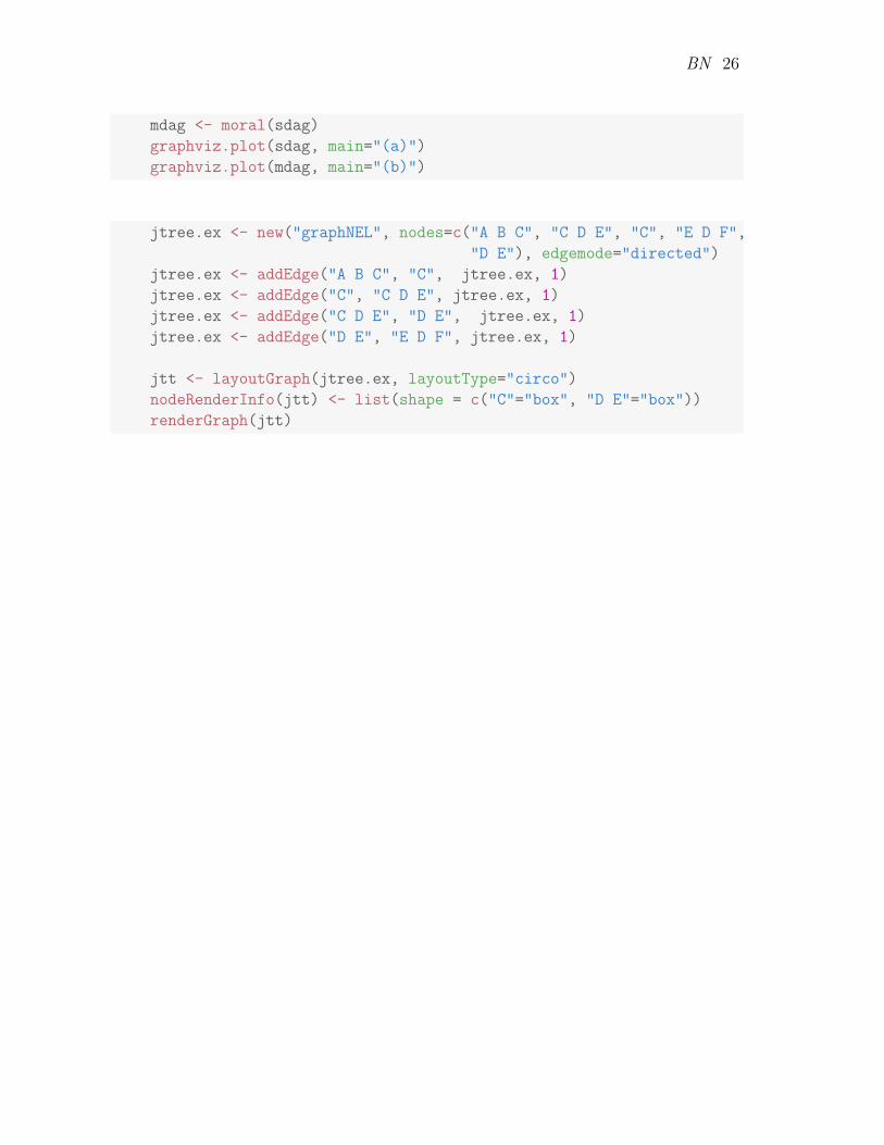
mdag <- moral(sdag)

graphviz.plot(sdag, main="(a)")

graphviz.plot(mdag, main="(b)")

jtree.ex <- new("graphNEL", nodes=c("A B C", "C D E", "C", "E D F",

"D E"), edgemode="directed")

jtree.ex <- addEdge("A B C", "C", jtree.ex, 1)

jtree.ex <- addEdge("C", "C D E", jtree.ex, 1)

jtree.ex <- addEdge("C D E", "D E", jtree.ex, 1)

jtree.ex <- addEdge("D E", "E D F", jtree.ex, 1)

jtt <- layoutGraph(jtree.ex, layoutType="circo")

nodeRenderInfo(jtt) <- list(shape = c("C"="box", "D E"="box"))

renderGraph(jtt)