Matrix presentation By DHEERAJ KATARIA
113
PREPARED BY:- DHEERAJ KATARIA(007)
-
Upload
dheeraj-kataria -
Category
Education
-
view
176 -
download
2
Transcript of Matrix presentation By DHEERAJ KATARIA

PREPARED BY:-
DHEERAJ KATARIA(007)
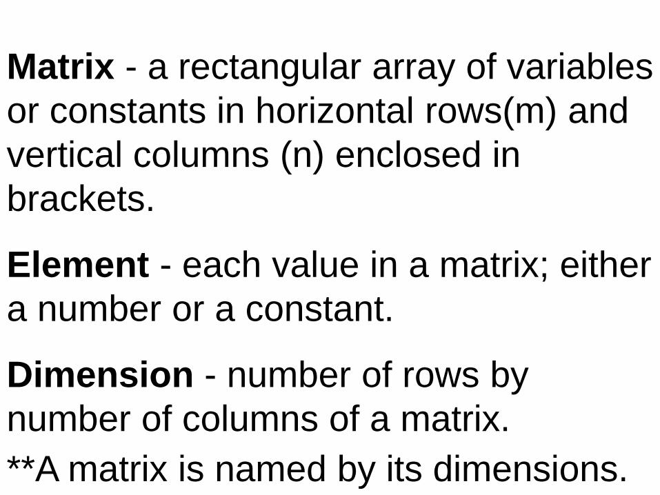
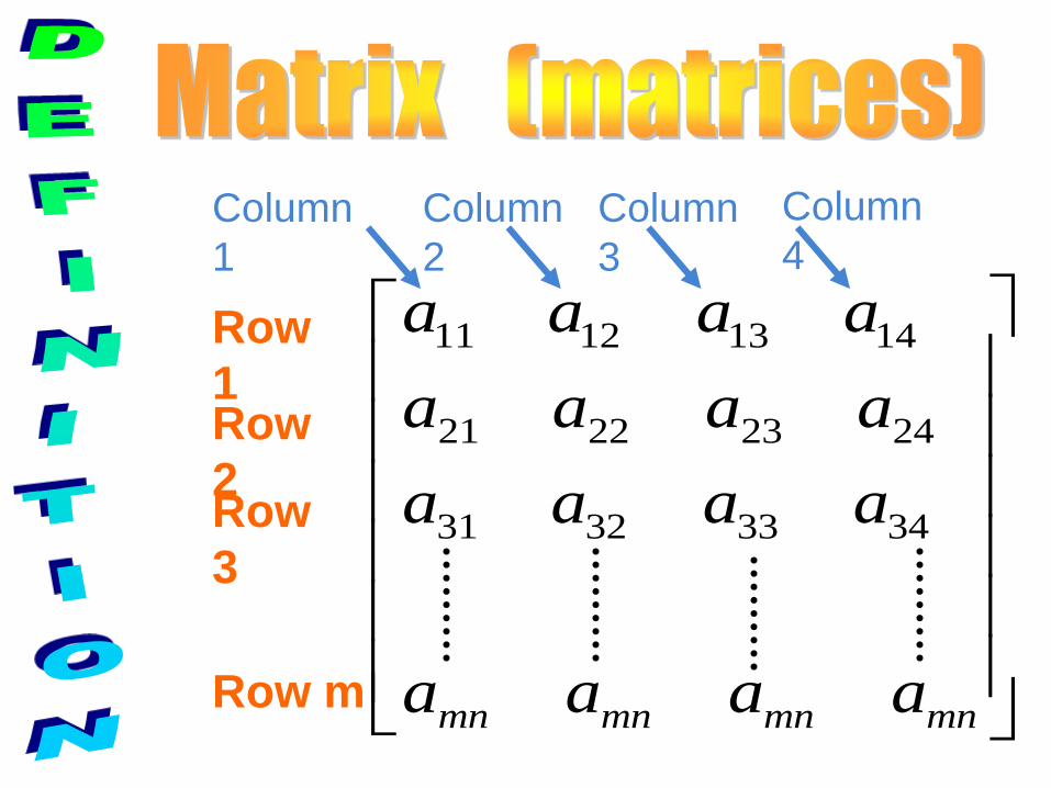
Matrix - a rectangular array of variables
or constants in horizontal rows(m) and
vertical columns (n) enclosed in
brackets.
Element - each value in a matrix; either
a number or a constant.
Dimension - number of rows by
number of columns of a matrix.
**A matrix is named by its dimensions.
11 12 13 14
21 22 23 24
31 32 33 34
mn mn mn mn
a a a a
a a a a
a a a a
a a a a
Row
1Row
2Row
3
Row m
Column
1
Column
2
Column
3
Column
4

Examples: Find the dimensions of each
matrix.
1. A =
2 1
0 5
4 8
2. B =
1
2
3
4
0 5 3 13. C =
2 0 9 6
Dimensions: 3x2 Dimensions: 4x1
Dimensions: 2x4
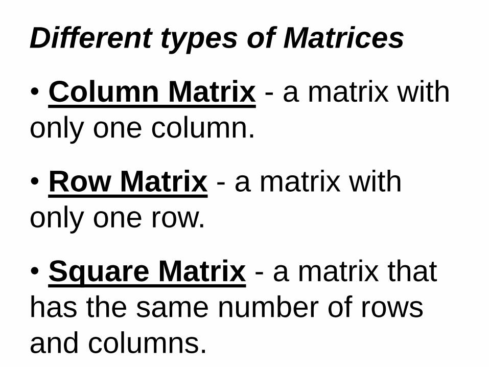
Different types of Matrices
• Column Matrix - a matrix with
only one column.
• Row Matrix - a matrix with
only one row.
• Square Matrix - a matrix that
has the same number of rows
and columns.

row
nmrows
mnmmm
n
n
n
aaaa
a
a
a
aaa
aaa
aaa
A
321
3
2
1
333231
232221
131211
A matrix is a rectangular array of numbers. We
subscript entries to tell their location in the array
Matrices are
identified by
their size.
Matrices and Rows
""
""
columnthj
rowthiaij

A matrix of m rows and n columns is
called a matrix with dimensions m x n.
2 3 4
1.) 11
2
3 8 9
2.) 2 5
6 7 8
103.)
7
4.) 3 4
2 X
3 3 X 3
2 X 11 X 2
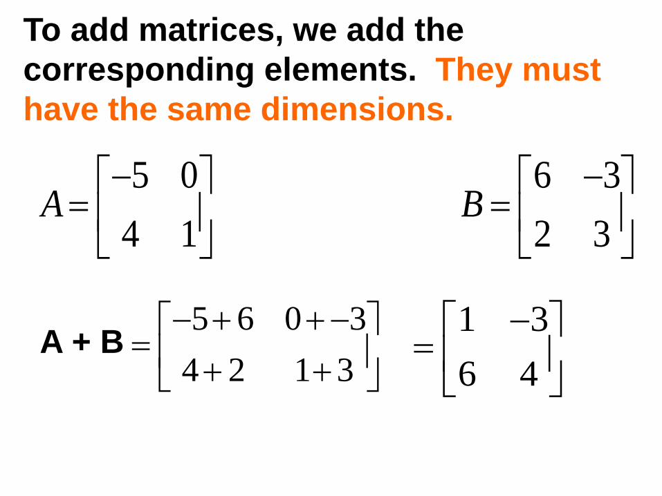
To add matrices, we add the
corresponding elements. They must
have the same dimensions.
5 0 6 3
4 1 2 3A B
A + B5 6 0 3
4 2 1 3
1 3
6 4
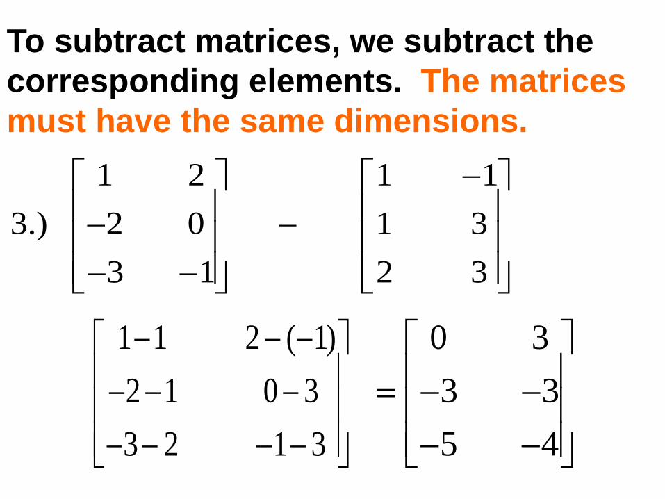
To subtract matrices, we subtract the
corresponding elements. The matrices
must have the same dimensions.
1 2 1 1
3.) 2 0 1 3
3 1 2 3
1 1 2 ( 1)
2 1 0 3
3 2 1 3
0 3
3 3
5 4
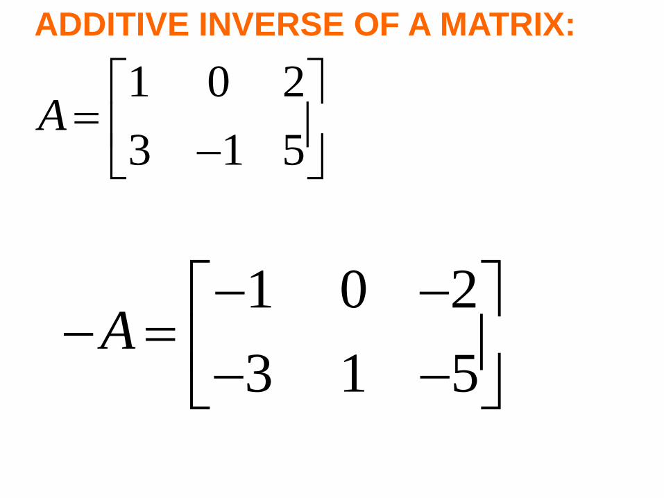
ADDITIVE INVERSE OF A MATRIX:
1 0 2
3 1 5A
1 0 2
3 1 5A
Equal Matrices - two matrices that
have the same dimensions and
each element of one matrix is equal
to the corresponding element of the
other matrix.
*The definition of equal matrices
can be used to find values when
elements of the matrices are
algebraic expressions.
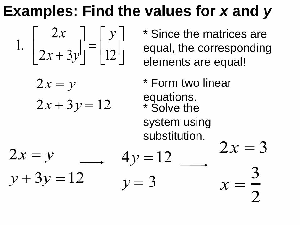
1. 2x
2x 3y
y
12
* Since the matrices are
equal, the corresponding
elements are equal!
* Form two linear
equations.2x y
2x 3y 12 * Solve the
system using
substitution.
Examples: Find the values for x and y
2x y
y 3y 12
4y 12
y 3
2x 3
x 3
2
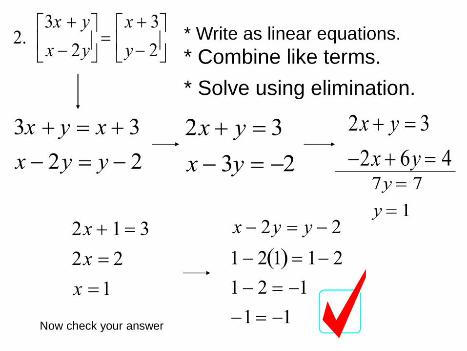
* Write as linear equations.2. 3x y
x 2y
x 3
y 2
7y 7
y 1
2x y 3
2x 6y 4
2x 1 3
2x 2
x 1
Now check your answer
* Combine like terms.
* Solve using elimination.
3x y x 3
x 2y y 2
x 2y y 2
1 2 1 1 2
1 2 1
1 1
2x y 3
x 3y 2
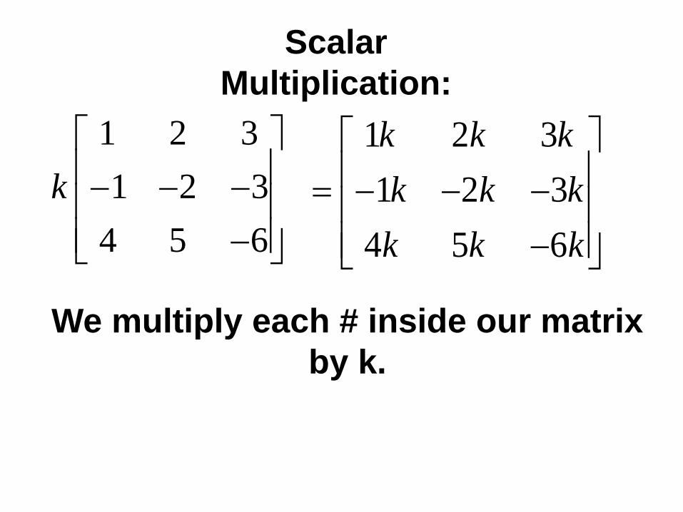
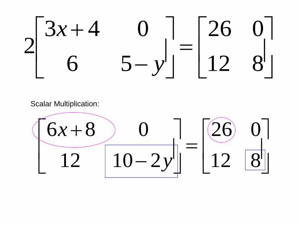
Scalar
Multiplication:
1 2 3
1 2 3
4 5 6
k
We multiply each # inside our matrix
by k.
1 2 3
1 2 3
4 5 6
k k k
k k k
k k k
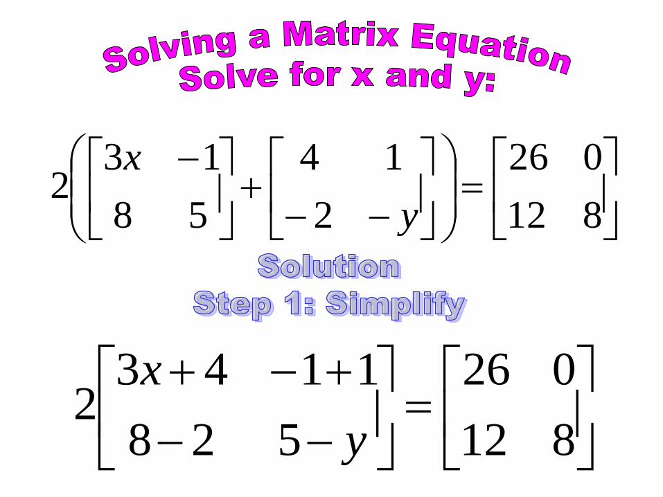
812
026
2
14
58
132
y
x
812
026
528
11432
y
x
812
026
56
0432
y
x
812
026
21012
086
y
x
Scalar Multiplication:
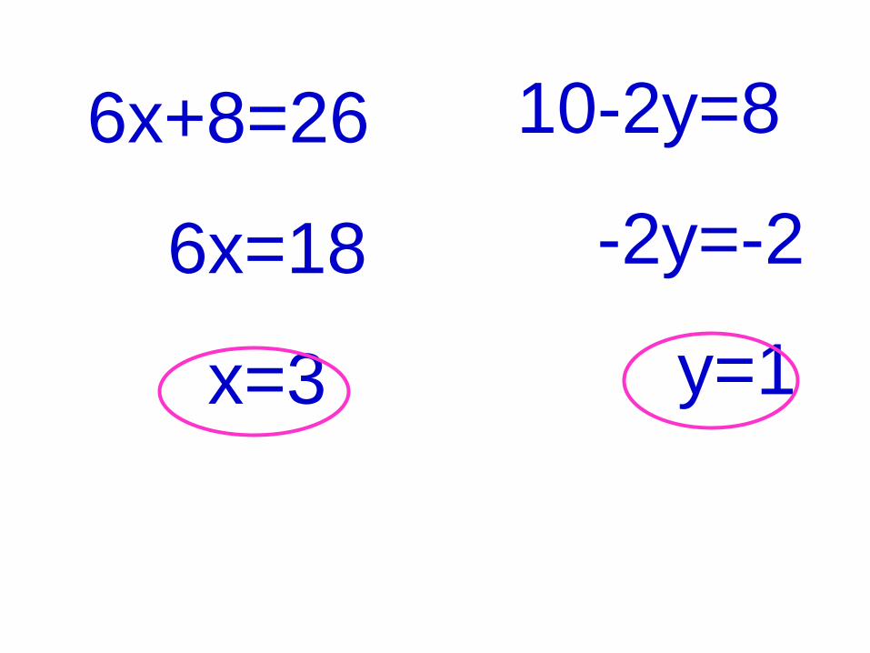
6x+8=26
6x=18
x=3
10-2y=8
-2y=-2
y=1
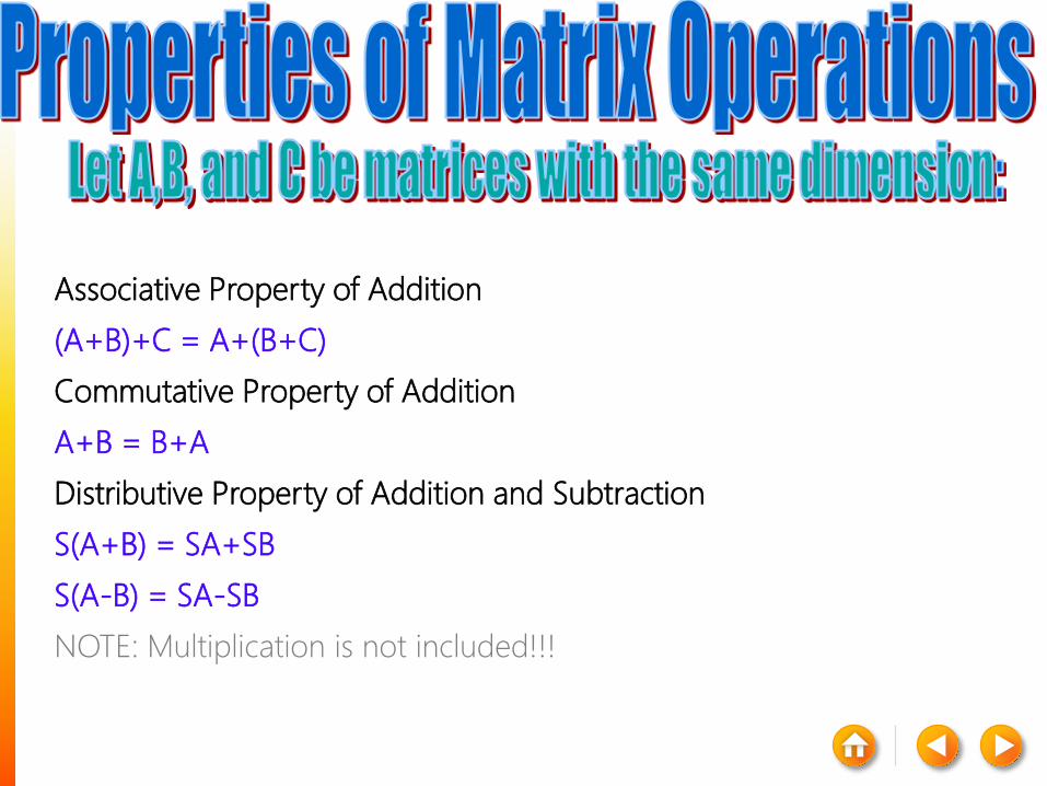
Associative Property of Addition
(A+B)+C = A+(B+C)
Commutative Property of Addition
A+B = B+A
Distributive Property of Addition and Subtraction
S(A+B) = SA+SB
S(A-B) = SA-SB
NOTE: Multiplication is not included!!!
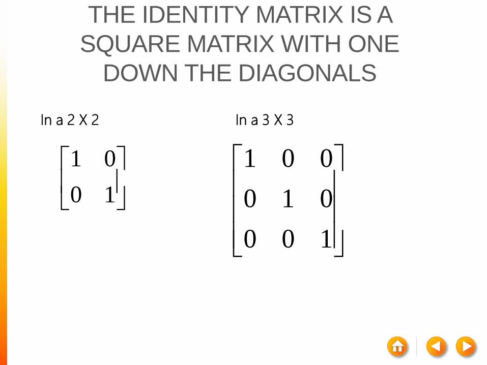
THE IDENTITY MATRIX IS A
SQUARE MATRIX WITH ONE
DOWN THE DIAGONALS
In a 2 X 2 In a 3 X 3
10
01
100
010
001

FINDING THE INVERSE OF A
MATRIX
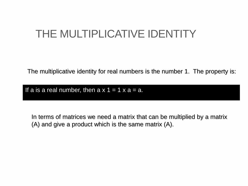
THE MULTIPLICATIVE IDENTITY
The multiplicative identity for real numbers is the number 1. The property is:
In terms of matrices we need a matrix that can be multiplied by a matrix
(A) and give a product which is the same matrix (A).
If a is a real number, then a x 1 = 1 x a = a.

THE INVERSE OF A MATRIX (A-1)
For an n n matrix A, there may be a B such
that AB = I = BA.
The inverse is analogous to a reciprocal
A matrix which has an inverse is nonsingular.
A matrix which does not have an inverse is
singular.
An inverse exists only if 0A

PROPERTIES OF INVERSE MATRICES
111 -- ABAB
'11 -AA'
AA 11-
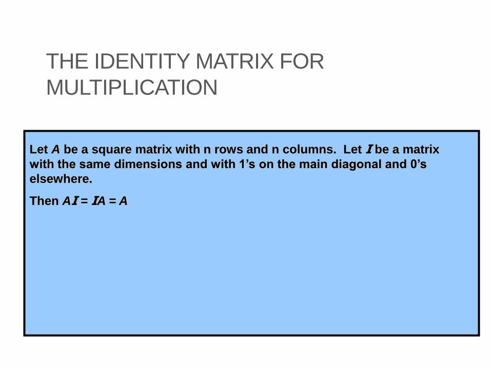
THE IDENTITY MATRIX FOR
MULTIPLICATION
Let A be a square matrix with n rows and n columns. Let I be a matrix
with the same dimensions and with 1’s on the main diagonal and 0’s
elsewhere.
Then AI = IA = A
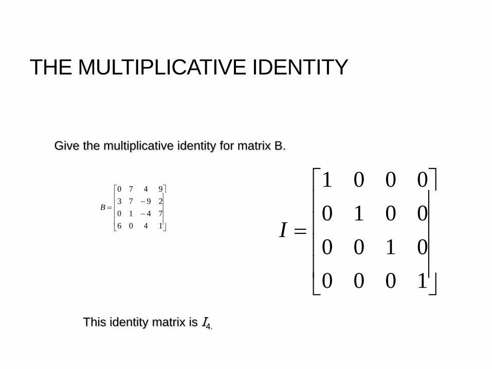
THE MULTIPLICATIVE IDENTITY
1406
7410
2973
9470
B
1000
0100
0010
0001
I
Give the multiplicative identity for matrix B.
This identity matrix is I4.
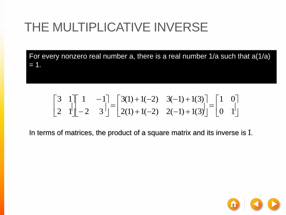
THE MULTIPLICATIVE INVERSE
10
01
)3(1)1(2)2(1)1(2
)3(1)1(3)2(1)1(3
32
11
12
13
For every nonzero real number a, there is a real number 1/a such that a(1/a)
= 1.
In terms of matrices, the product of a square matrix and its inverse is I.
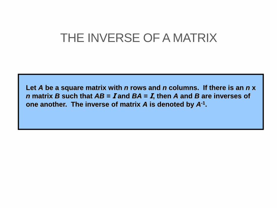
THE INVERSE OF A MATRIX
Let A be a square matrix with n rows and n columns. If there is an n x
n matrix B such that AB = I and BA = I, then A and B are inverses of
one another. The inverse of matrix A is denoted by A-1.

THE INVERSE OF A MATRIX
23
35
53
32BandA
To show that matrices are inverses of one another, show that the
multiplication of the matrices is commutative and results in the identity
matrix.
Show that A and B are inverses.

THE INVERSE OF A MATRIX
10
01
)2(5)3(3)3(5)5(3
)2(3)3(2)3(3)5(2
23
35
53
32AB
and
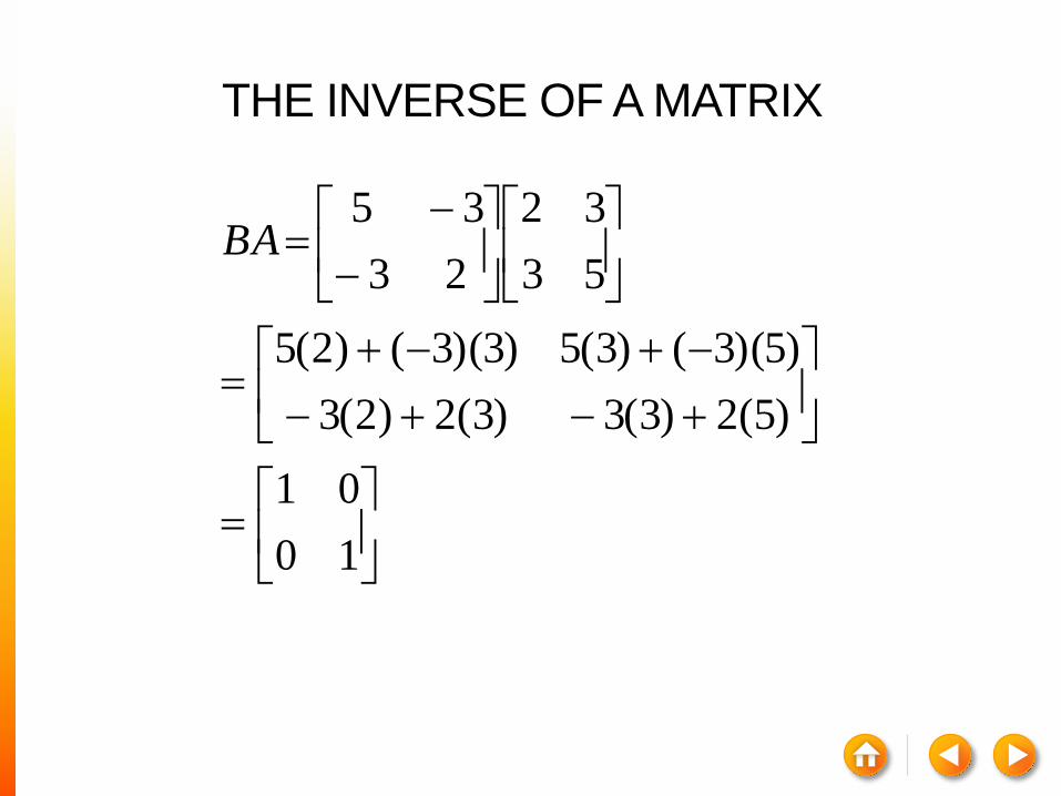
THE INVERSE OF A MATRIX
10
01
)5(2)3(3)3(2)2(3
)5)(3()3(5)3)(3()2(5
53
32
23
35BA
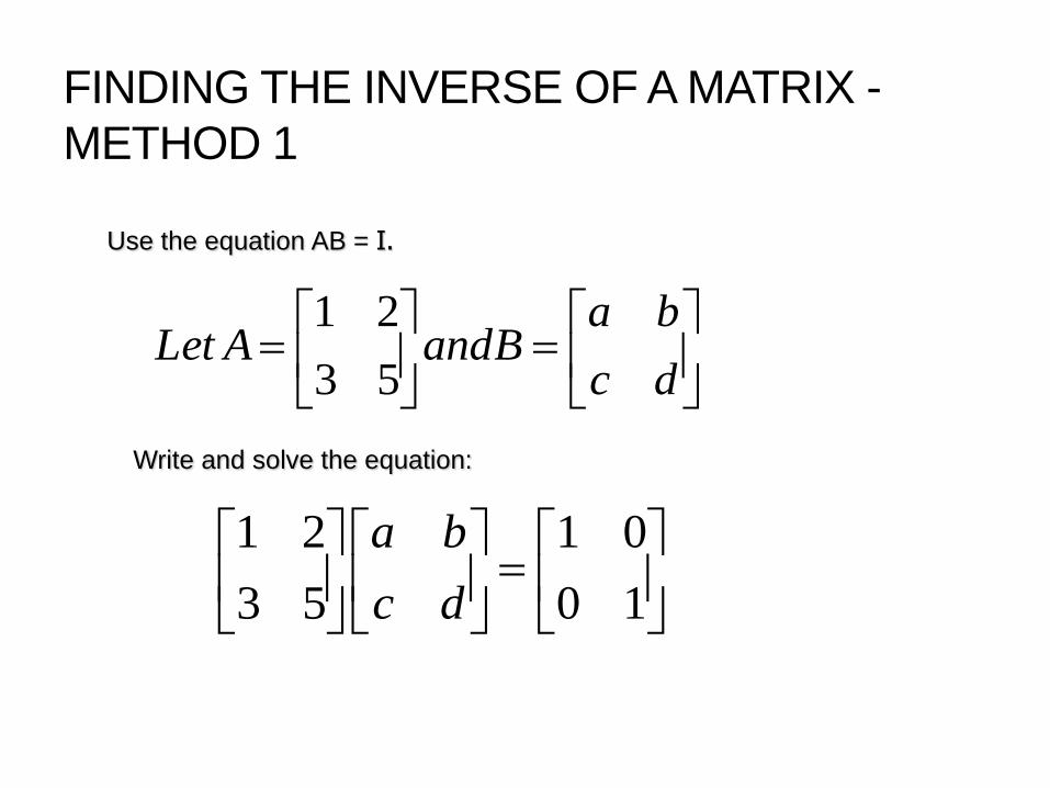
FINDING THE INVERSE OF A MATRIX -
METHOD 1
dc
baBandALet
53
21
10
01
53
21
dc
ba
Use the equation AB = I.
Write and solve the equation:

INVERSES – METHOD 1, CONT.
10
01
53
21
dc
ba
10
01
5353
22
dbca
dbca
1235
153
02
053
12
dandbcanda
db
db
ca
ca

INVERSES – METHOD 1, CONT.
13
25
10
01
)1(5)2(3)3(5)5(3
)1(2)2(1)3(2)5(1
13
25
53
21
So the inverse of A =
We can check this by multiplying A x A-1
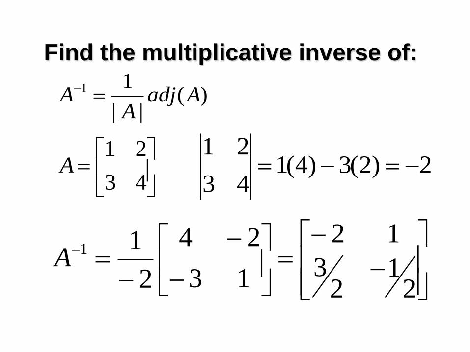
Find the multiplicative inverse of:
43
21A
21
23
12
13
24
2
11A
2)2(3)4(143
21
)(||
11 AadjA
A
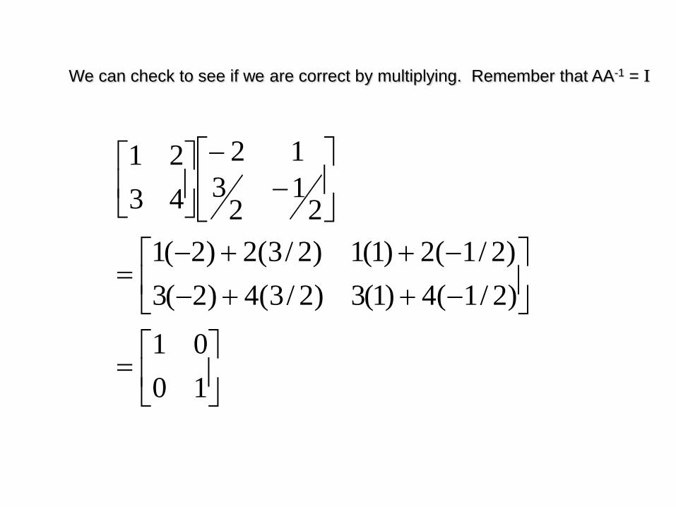
We can check to see if we are correct by multiplying. Remember that AA-1 = I
10
01
)2/1(4)1(3)2/3(4)2(3
)2/1(2)1(1)2/3(2)2(1
21
23
12
43
21
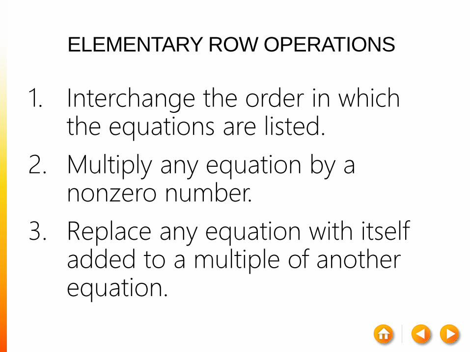
ELEMENTARY ROW OPERATIONS
1. Interchange the order in which the equations are listed.
2. Multiply any equation by a nonzero number.
3. Replace any equation with itself added to a multiple of another equation.

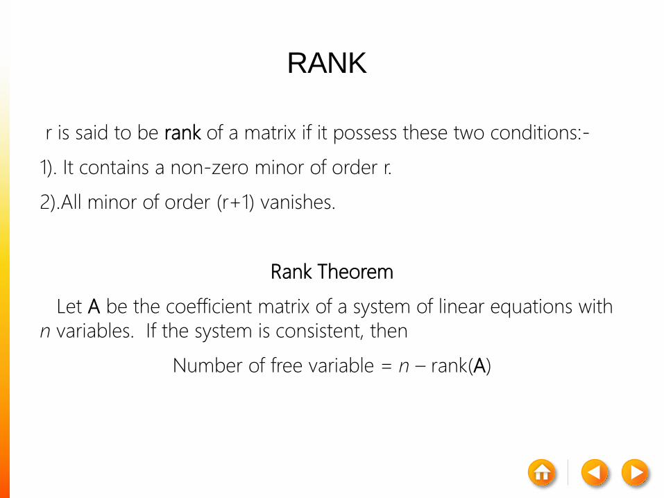
RANK
r is said to be rank of a matrix if it possess these two conditions:-
1). It contains a non-zero minor of order r.
2).All minor of order (r+1) vanishes.
Rank Theorem
Let A be the coefficient matrix of a system of linear equations with
n variables. If the system is consistent, then
Number of free variable = n – rank(A)
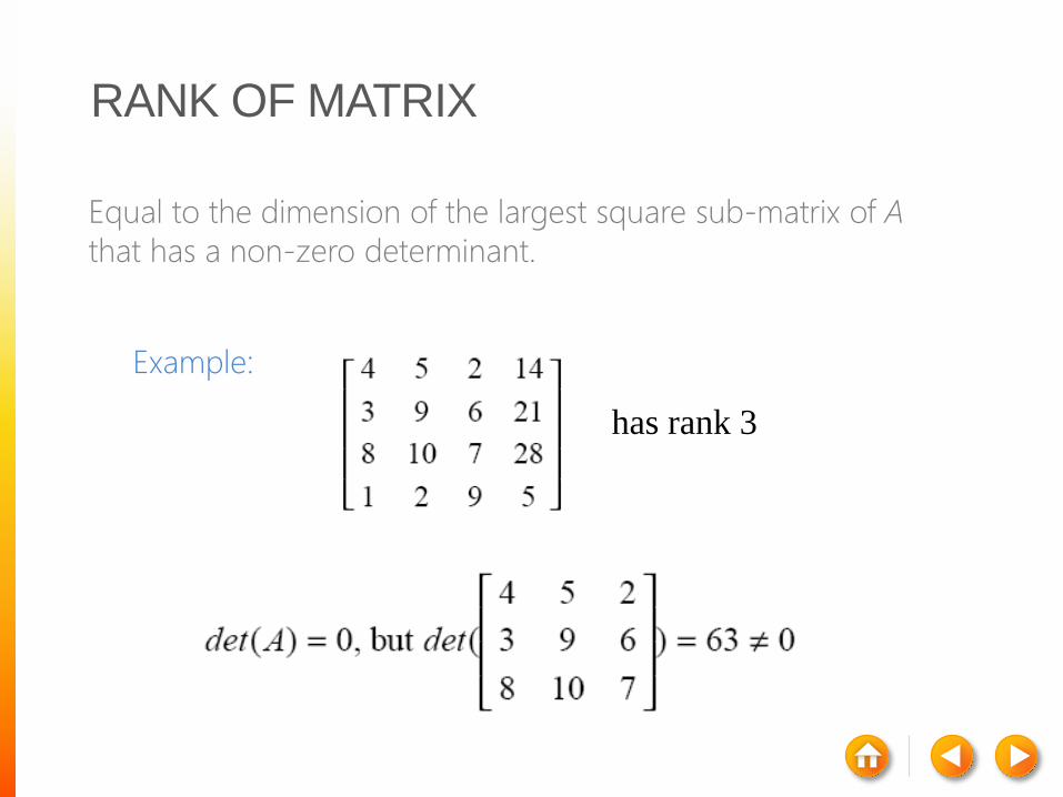
RANK OF MATRIX
Equal to the dimension of the largest square sub-matrix of A
that has a non-zero determinant.
Example:
has rank 3
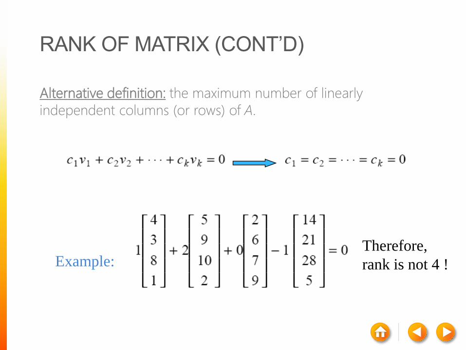
RANK OF MATRIX (CONT’D)
Alternative definition: the maximum number of linearly
independent columns (or rows) of A.
Therefore,
rank is not 4 !Example:
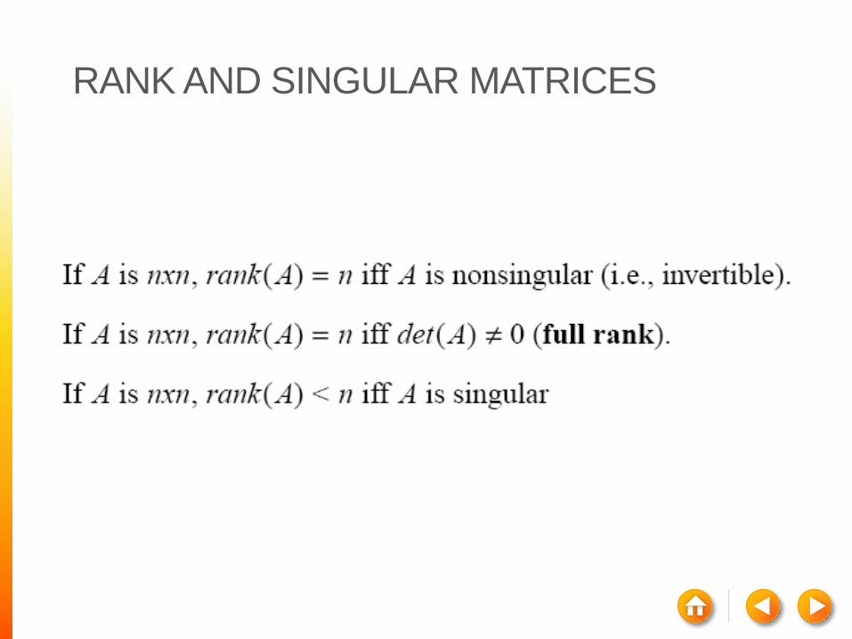
RANK AND SINGULAR MATRICES

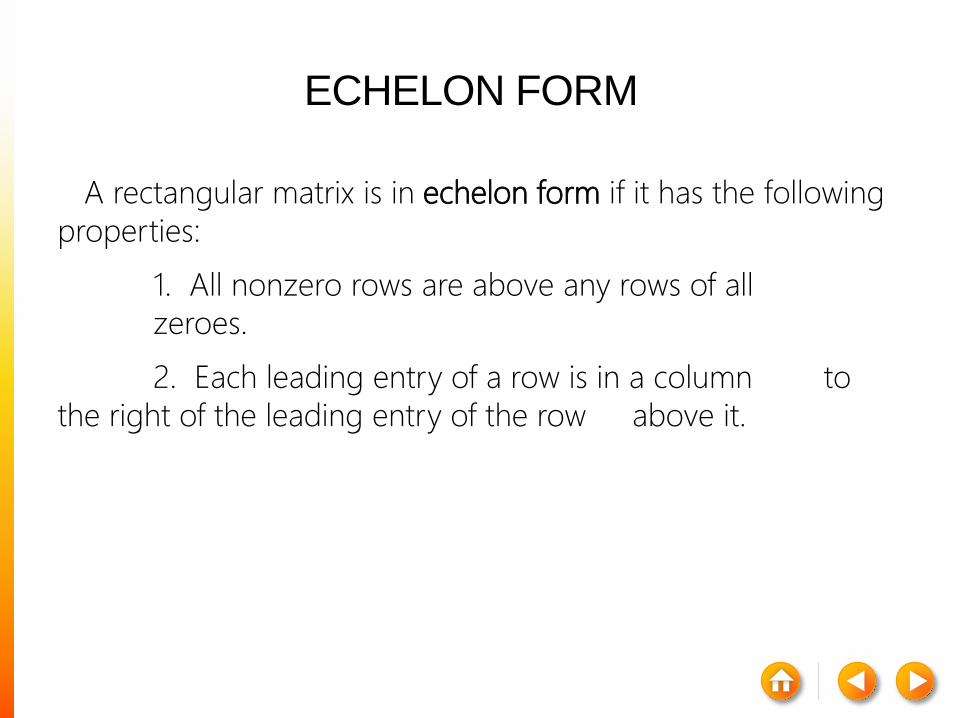
ECHELON FORM
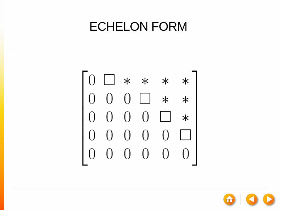
A rectangular matrix is in echelon form if it has the following
properties:
1. All nonzero rows are above any rows of all
zeroes.
2. Each leading entry of a row is in a column to
the right of the leading entry of the row above it.
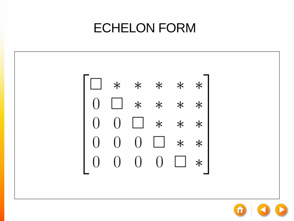
ECHELON FORM
ECHELON FORM

EXAMPLE
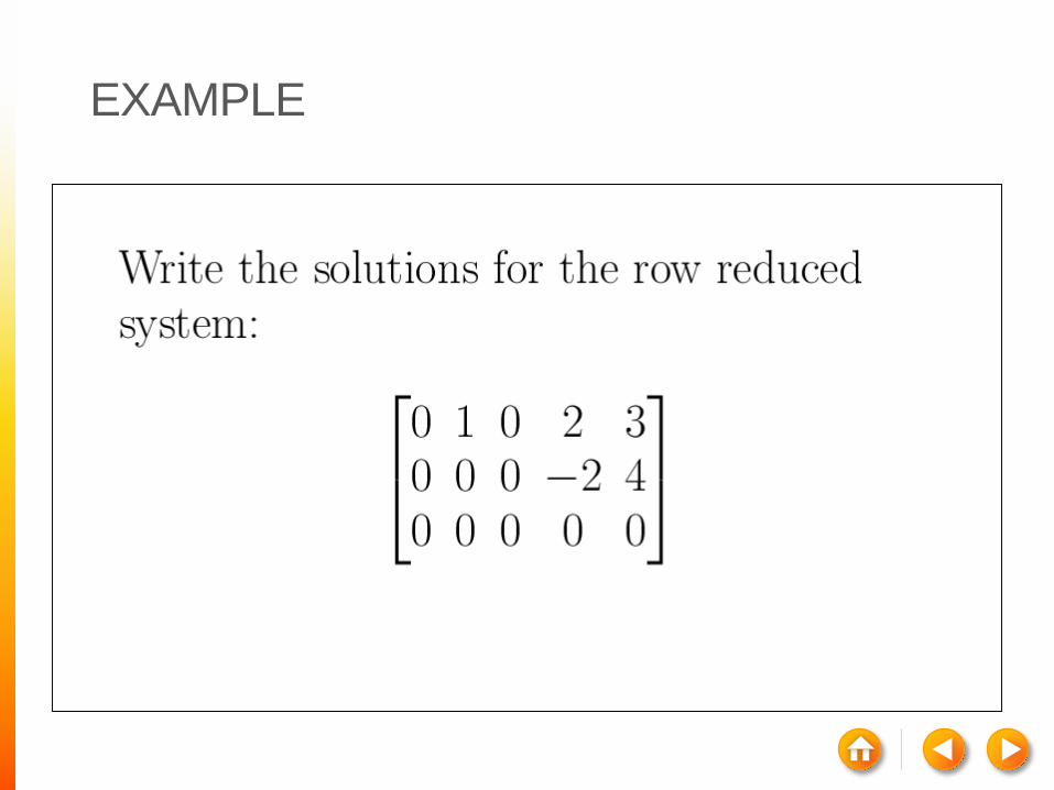
EXAMPLE
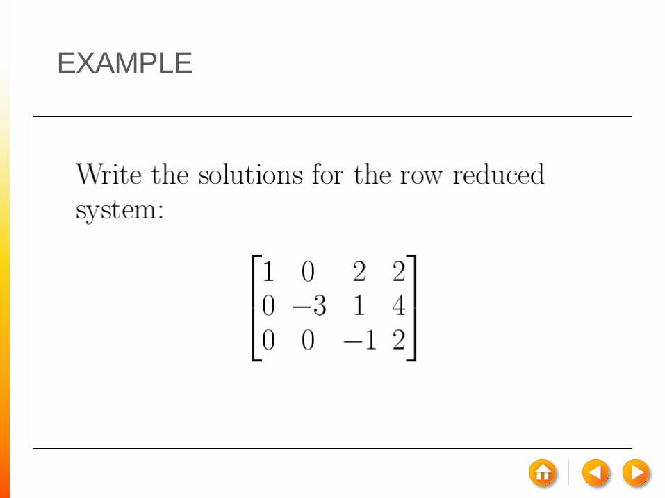
EXAMPLE
ECHELON FORM
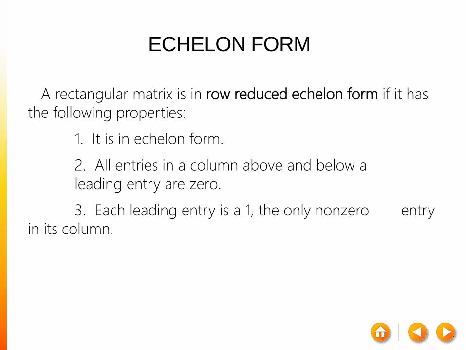
A rectangular matrix is in row reduced echelon form if it has
the following properties:
1. It is in echelon form.
2. All entries in a column above and below a
leading entry are zero.
3. Each leading entry is a 1, the only nonzero entry
in its column.
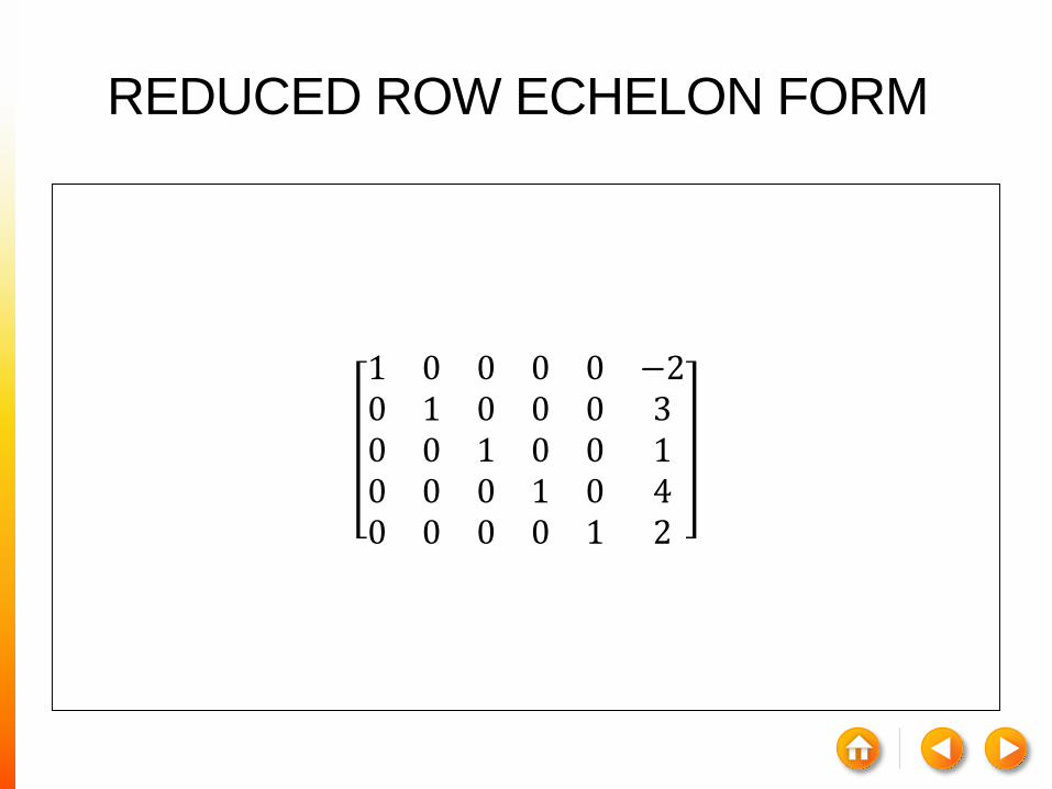
1 0 0 0 0 −20 1 0 0 0 30 0 1 0 0 10 0 0 1 0 40 0 0 0 1 2
REDUCED ROW ECHELON FORM
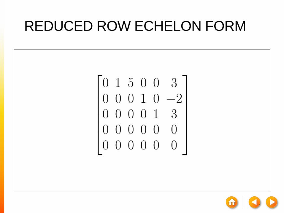
REDUCED ROW ECHELON FORM
HOMOGENEOUS SYSTEM
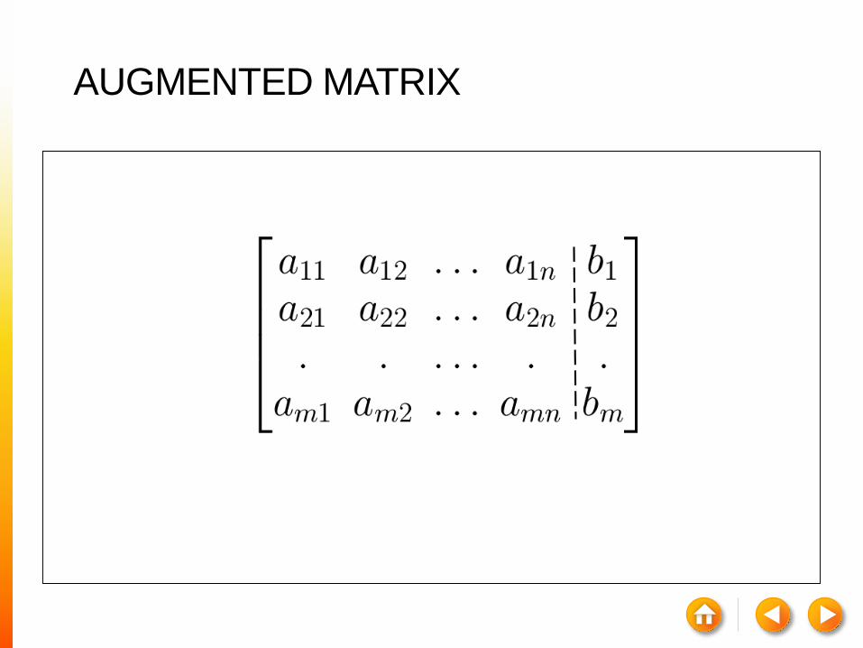
AUGMENTED MATRIX

Solve the system of equations using Gauss-Jordan Method
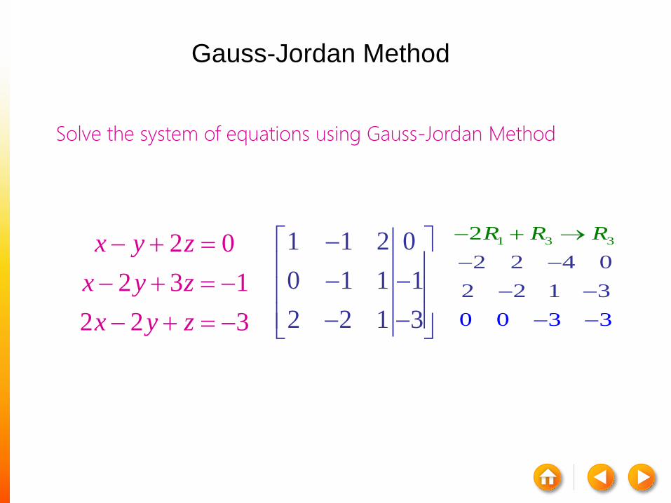
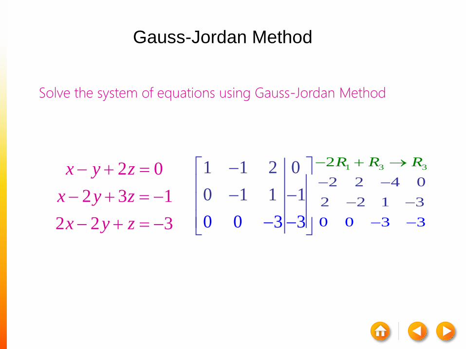
2 0
2 3 1
2 2 3
x y z
x y z
x y z
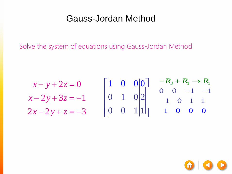
Gauss-Jordan Method

Solve the system of equations using Gauss-Jordan Method
2 0
2 3 1
2 2 3
x y z
x y z
x y z
1 2 2
1 1 2
0 1 1
0
1
1
2 3 1
R R R
0 1 1
1 1 2 0
2 3
1
2 1
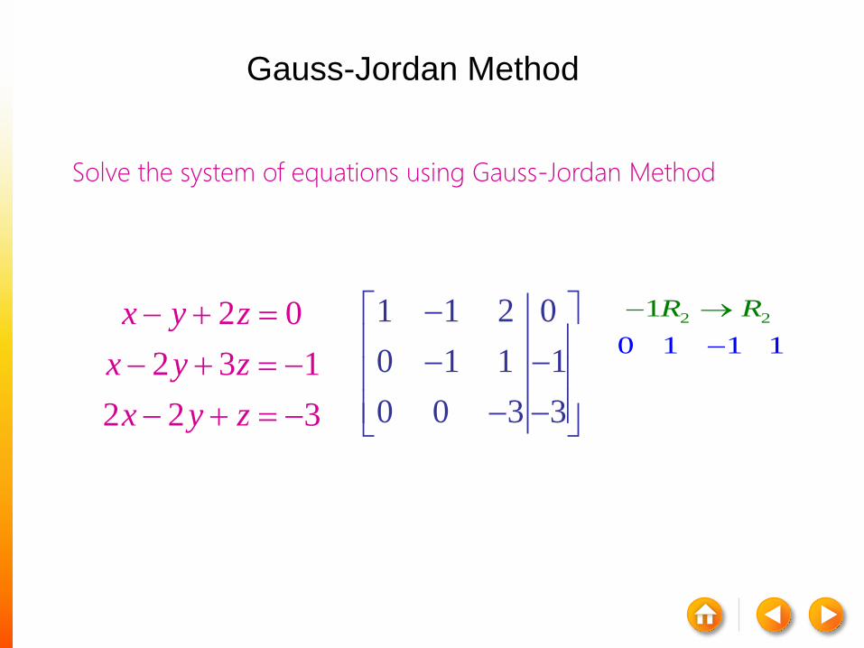
Gauss-Jordan Method
Solve the system of equations using Gauss-Jordan Method
2 0
2 3 1
2 2 3
x y z
x y z
x y z
1 1 2 0
0 1 1 1
2 2 1 3
1 3 3
2 2 4 0
2 2 1 3
3
2
0 0 3
R R R
Gauss-Jordan Method
Solve the system of equations using Gauss-Jordan Method
2 0
2 3 1
2 2 3
x y z
x y z
x y z
1 3 3
2 2 4 0
2 2 1 3
3
2
0 0 3
R R R
0 0
1 1 2 0
0 1 1
3
1
3
Gauss-Jordan Method
Solve the system of equations using Gauss-Jordan Method
2 0
2 3 1
2 2 3
x y z
x y z
x y z
1 1 2 0
0 1 1 1
0 0 3 3
2 2
0
1
1 1 1
R R
Gauss-Jordan Method

Solve the system of equations using Gauss-Jordan Method
2 0
2 3 1
2 2 3
x y z
x y z
x y z
2 2
0
1
1 1 1
R R
0 1 1 1
1 1 2 0
0 0 3 3
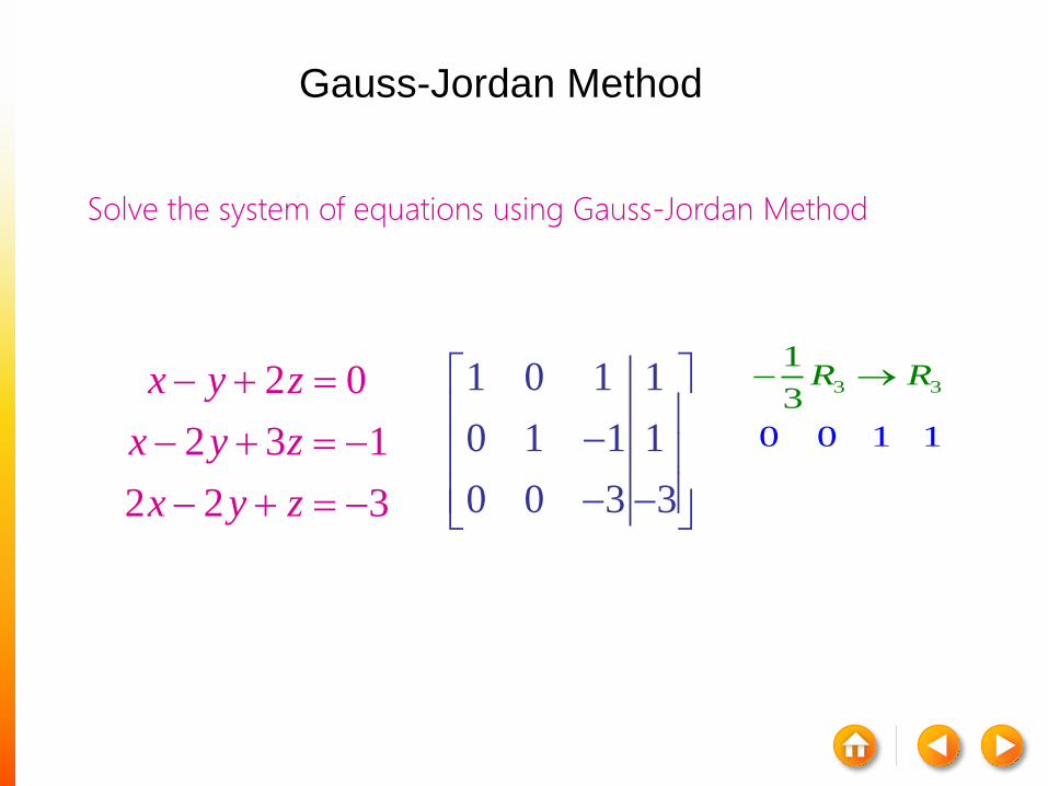
Gauss-Jordan Method

Solve the system of equations using Gauss-Jordan Method
2 0
2 3 1
2 2 3
x y z
x y z
x y z
1 1 2 0
0 1 1 1
0 0 3 3
2 1 1
0 1 1 1
1
1 0 1 1
1 2 0
R R R
Gauss-Jordan Method

Solve the system of equations using Gauss-Jordan Method
2 0
2 3 1
2 2 3
x y z
x y z
x y z
2 1 1
0 1 1 1
1
1 0 1 1
1 2 0
R R R
0 1 1 1
0 0 3 3
1 0 1 1
Gauss-Jordan Method
Solve the system of equations using Gauss-Jordan Method
2 0
2 3 1
2 2 3
x y z
x y z
x y z
1 0 1 1
0 1 1 1
0 0 3 3
3 3
1
3
0 0 1 1
R R
Gauss-Jordan Method

Solve the system of equations using Gauss-Jordan Method
2 0
2 3 1
2 2 3
x y z
x y z
x y z
3 3
1
3
0 0 1 1
R R 1 0 1 1
0 1 11
0 0 1 1
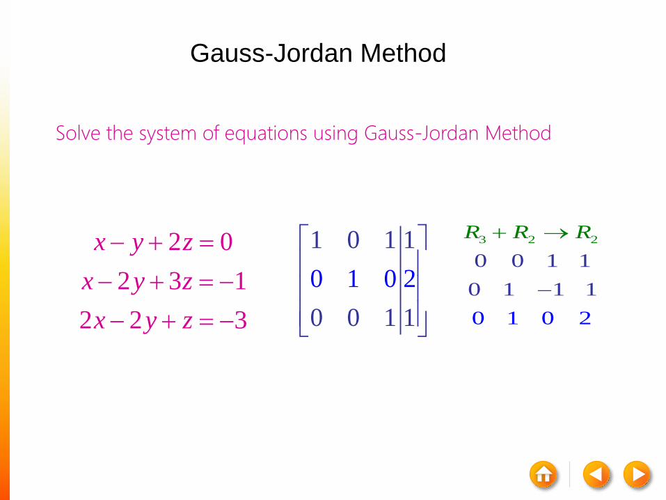
Gauss-Jordan Method

Solve the system of equations using Gauss-Jordan Method
2 0
2 3 1
2 2 3
x y z
x y z
x y z
1 0 1 1
0 1 11
0 0 1 1
3 2 2
0 0 1 1
0 1 1
1
1
0 0 2
R R R
Gauss-Jordan Method
Solve the system of equations using Gauss-Jordan Method
2 0
2 3 1
2 2 3
x y z
x y z
x y z
3 2 2
0 0 1 1
0 1 1
1
1
0 0 2
R R R
1 0 1 1
0 0 1 1
0 1 0 2
Gauss-Jordan Method
Solve the system of equations using Gauss-Jordan Method
2 0
2 3 1
2 2 3
x y z
x y z
x y z
1 0 1 1
0 1 0 2
0 0 1 1
3 1 1
0
1 0
0 1
0 0
1
1 0 1 1
R R R
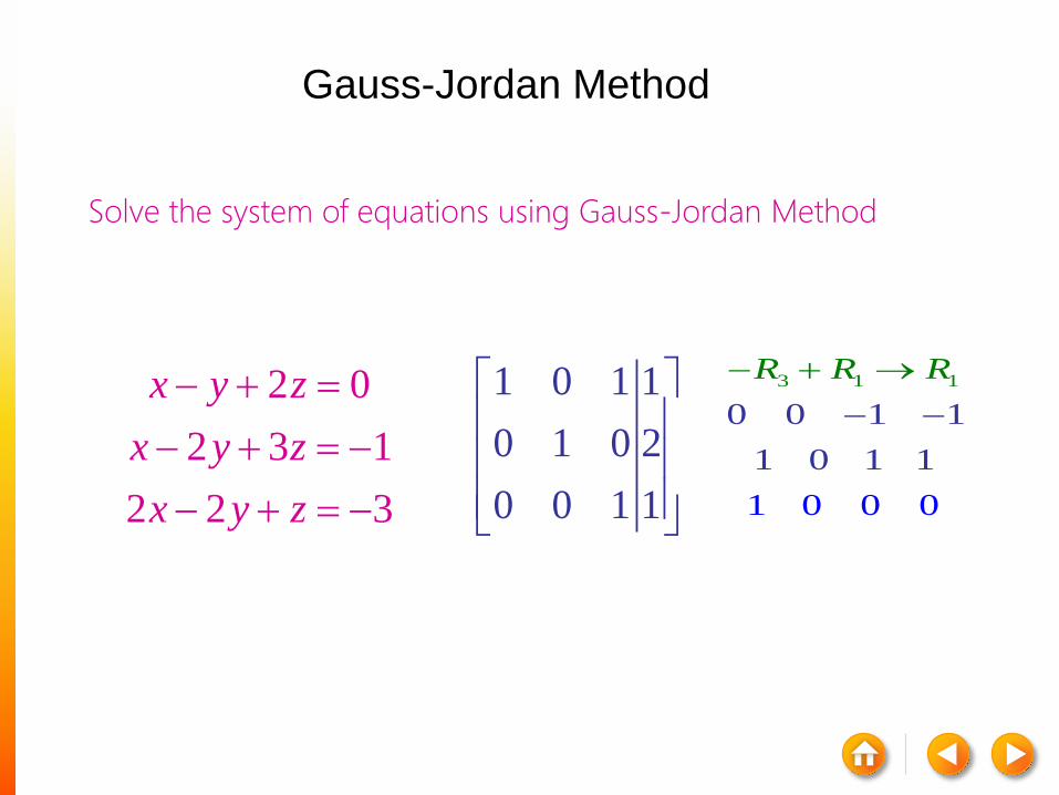
Gauss-Jordan Method
Solve the system of equations using Gauss-Jordan Method
2 0
2 3 1
2 2 3
x y z
x y z
x y z
3 1 1
0
1 0
0 1
0 0
1
1 0 1 1
R R R
0 1 0 2
0 0 1 1
1 0 0 0
Gauss-Jordan Method
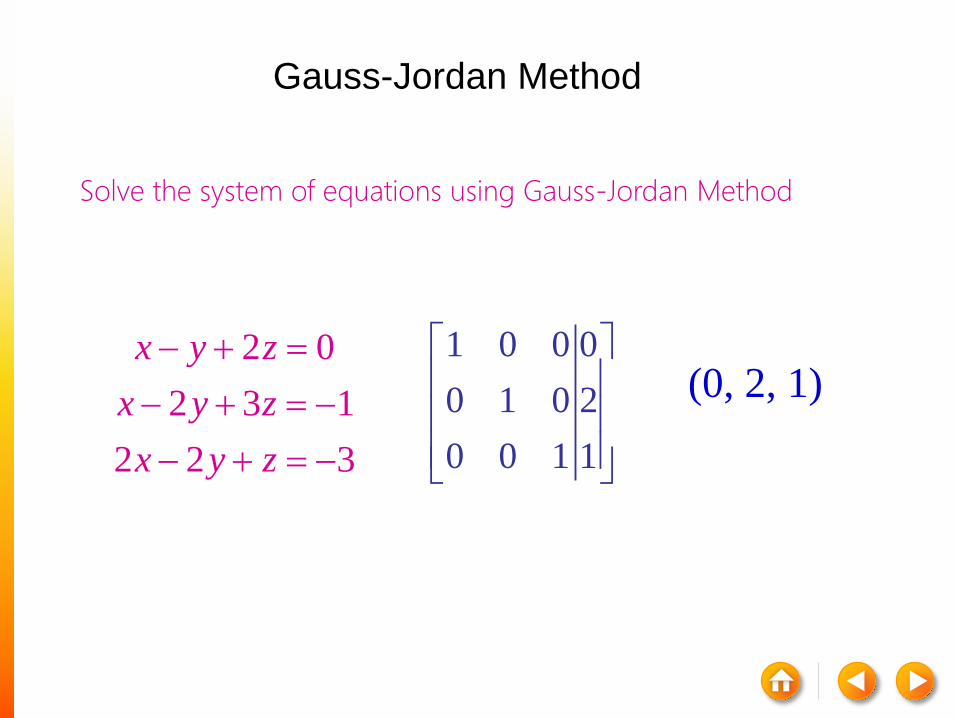
Solve the system of equations using Gauss-Jordan Method
2 0
2 3 1
2 2 3
x y z
x y z
x y z
1 0 0 0
0 1 0 2
0 0 1 1
(0, 2, 1)
Gauss-Jordan Method
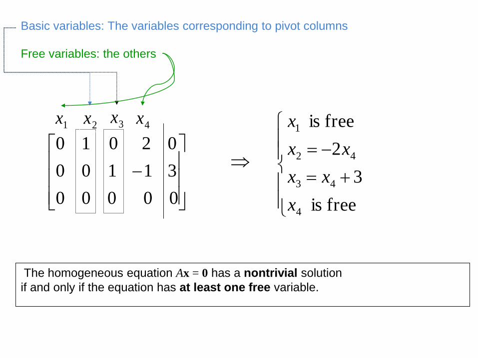
The homogeneous equation Ax = 0 has a nontrivial solution
if and only if the equation has at least one free variable.
Basic variables: The variables corresponding to pivot columns
00000
31100
02010
1x 2x 3x4x
Free variables: the others
free is
3
2
free is
4
43
42
1
x
xx
xx
x

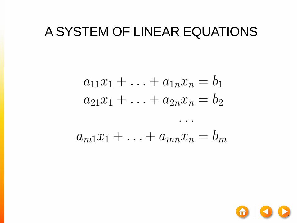
A SYSTEM OF LINEAR EQUATIONS
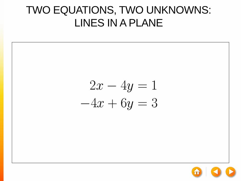
TWO EQUATIONS, TWO UNKNOWNS:
LINES IN A PLANE
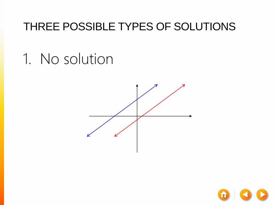
THREE POSSIBLE TYPES OF SOLUTIONS
1. No solution

THREE POSSIBLE TYPES OF SOLUTIONS
1. A unique solution

THREE POSSIBLE TYPES OF SOLUTIONS
1. Infinitely many solutions

THREE EQUATIONS,THREE
UNKNOWNS:
PLANES IN SPACE

Definition of Homogeneous
A system of linear equations is said to be homogeneous
if it can be written in the form Ax = 0, where A is an
matrix and 0 is the zero vector in Rm.
nm
Example:
023
034
0452
321
321
321
xxx
xxx
xxx
Note: Every homogeneous linear system is consistent.
i.e. The homogeneous system Ax = 0 has at least one solution, namely the trivial
solution, x = 0.

The homogeneous equation Ax = 0 has a nontrivial solution
if and only if the equation has at least one free variable.
Basic variables: The variables corresponding to pivot columns
00000
31100
02010
1x 2x 3x4x
Free variables: he others
free is
3
2
free is
4
43
42
1
x
xx
xx
x
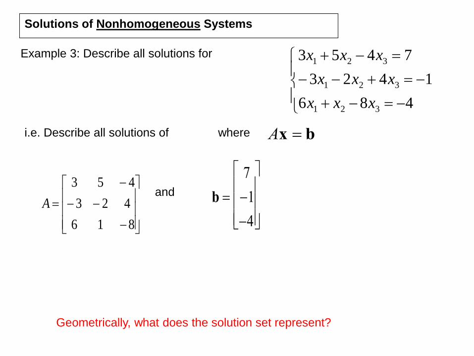
Example 3: Describe all solutions for
486
1423
7453
321
321
321
xxx
xxx
xxx
Solutions of Nonhomogeneous Systems
i.e. Describe all solutions of where
Ax b
816
423
453
Aand
b
7
1
4
Geometrically, what does the solution set represent?
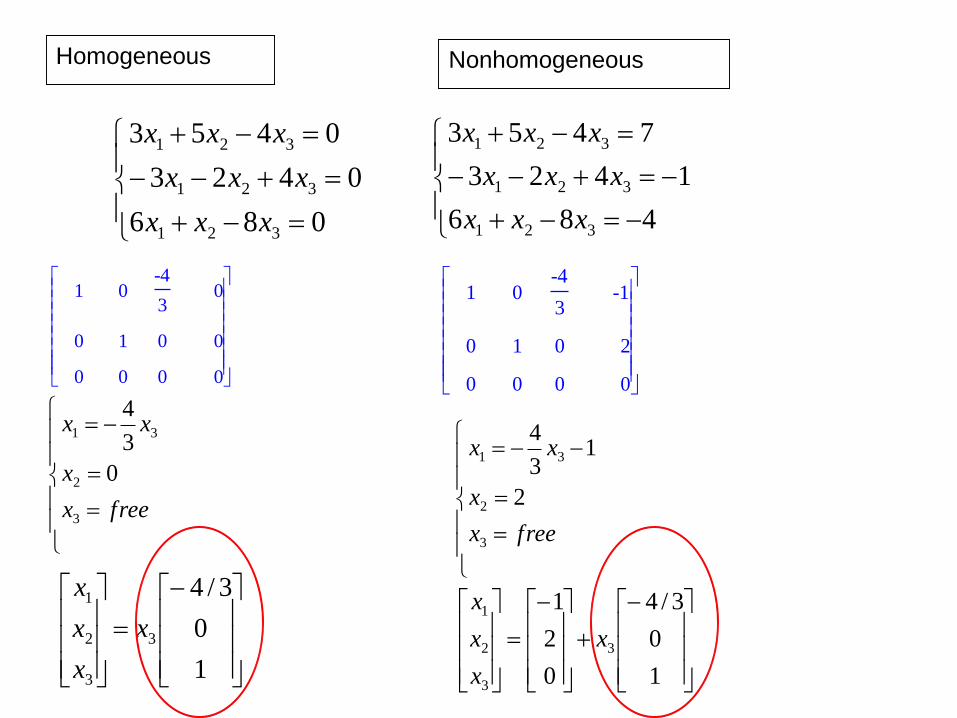
Homogeneous
086
0423
0453
321
321
321
xxx
xxx
xxx
Nonhomogeneous
486
1423
7453
321
321
321
xxx
xxx
xxx
1 0-4
30
0 1 0 0
0 0 0 0
1 0-4
3-1
0 1 0 2
0 0 0 0
freex
x
xx
3
2
31
0
3
4
freex
x
xx
3
2
31
2
13
4
1
0
3/4
3
3
2
1
x
x
x
x
1
0
3/4
0
2
1
3
3
2
1
x
x
x
x
THEOREM

CRAMER’S RULE
Example:
Solve the system: 3x - 2y = 10
4x + y = 6
10 2
6 1 222
3 2 11
4 1
x
3 10
4 6 222
3 2 11
4 1
y
The solution is
(2, -2)

CRAMER’S RULE
●Example:Solve the system 3x - 2y + z = 9
x + 2y - 2z = -5x + y - 4z = -2
x
9 2 1
5 2 2
2 1 4
3 2 1
1 2 2
1 1 4
23
23 1 y
3 9 1
1 5 2
1 2 4
3 2 1
1 2 2
1 1 4
69
23 3

CRAMER’S RULE
Example, continued: 3x - 2y + z = 9 x + 2y - 2z = -5
x + y - 4z = -2
z
3 2 9
1 2 5
1 1 2
3 2 1
1 2 2
1 1 4
0
23 0
The solution is
(1, -3, 0)

GAUSSIAN ELIMINATION
To solve a system of equations using Gaussian elimination with matrices, we use the same rules as before.
1. Interchange any two rows.
2. Multiply each entry in a row by the same nonzero constant.
3. Add a nonzero multiple of one row to another row.
A method to solve simultaneous linear equations of the form [A][X]=[C]
Two steps1. Forward Elimination
2. Back Substitution
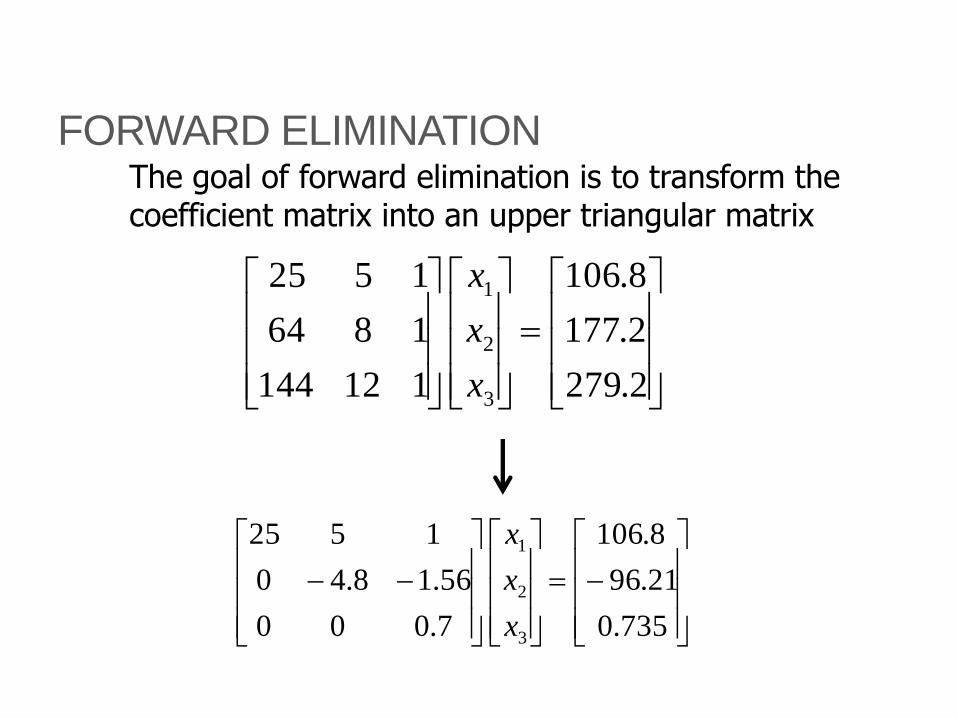
FORWARD ELIMINATION
735.0
21.96
8.106
7.000
56.18.40
1525
3
2
1
x
x
x
2.279
2.177
8.106
112144
1864
1525
3
2
1
x
x
x
The goal of forward elimination is to transform the coefficient matrix into an upper triangular matrix

FORWARD ELIMINATION
A set of n equations and n unknowns
11313212111 ... bxaxaxaxa nn
22323222121 ... bxaxaxaxa nn
nnnnnnn bxaxaxaxa ...332211
. .
. .
. .
(n-1) steps of forward elimination
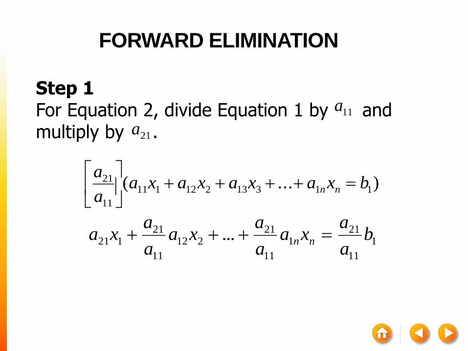
Step 1 For Equation 2, divide Equation 1 by and multiply by .
)...( 11313212111
11
21 bxaxaxaxaa
ann
1
11
211
11
21212
11
21121 ... b
a
axa
a
axa
a
axa nn
11a
21a
FORWARD ELIMINATION

FORWARD ELIMINATION
1
11
211
11
21212
11
21121 ... b
a
axa
a
axa
a
axa nn
22323222121 ... bxaxaxaxa nn
1
11
2121
11
212212
11
2122 ... b
a
abxa
a
aaxa
a
aa nnn
'
2
'
22
'
22 ... bxaxa nn
Subtract the result from Equation 2.
−_________________________________________________
or

Repeat this procedure for the remaining equations to reduce the set of equations as
11313212111 ... bxaxaxaxa nn
'
2
'
23
'
232
'
22 ... bxaxaxa nn
'
3
'
33
'
332
'
32 ... bxaxaxa nn
''
3
'
32
'
2 ... nnnnnn bxaxaxa
. . .
. . .
. . .
End of Step 1
FORWARD ELIMINATION
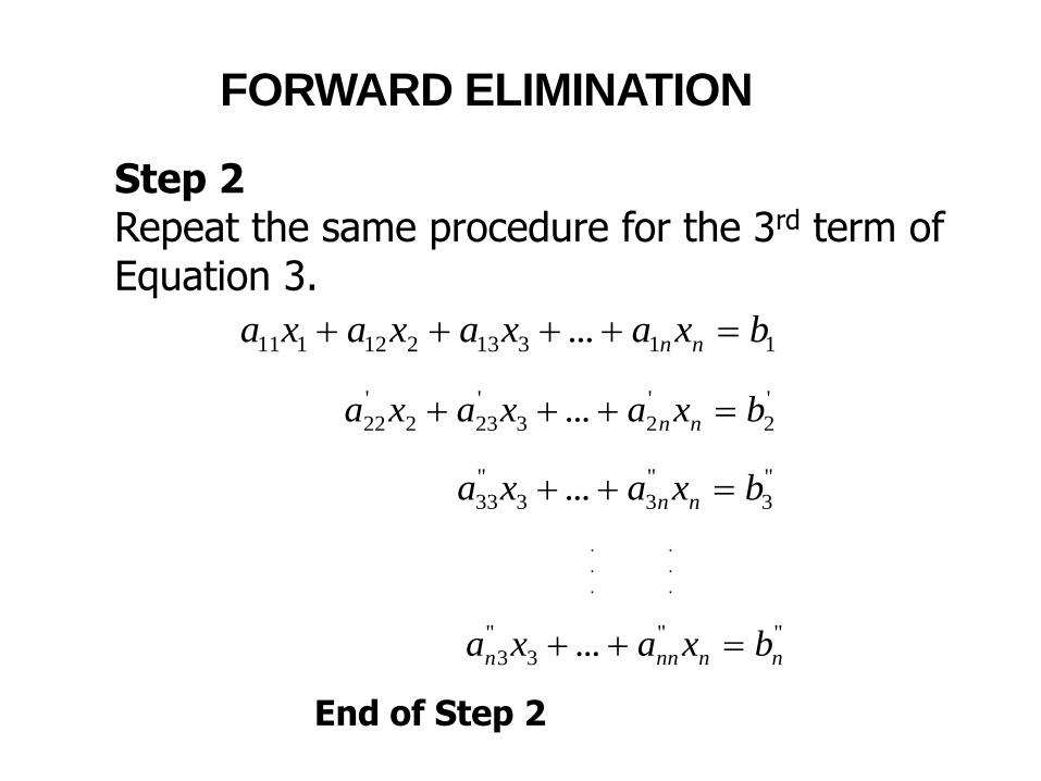
Step 2Repeat the same procedure for the 3rd term of Equation 3.
11313212111 ... bxaxaxaxa nn
'
2
'
23
'
232
'
22 ... bxaxaxa nn
"
3
"
33
"
33 ... bxaxa nn
""
3
"
3 ... nnnnn bxaxa
. .
. .
. .
End of Step 2
FORWARD ELIMINATION

At the end of (n-1) Forward Elimination steps, the system of equations will look like
'
2
'
23
'
232
'
22 ... bxaxaxa nn
"
3
"
33
"
33 ... bxaxa nn
11 n
nn
n
nn bxa
. .
. .
. .
11313212111 ... bxaxaxaxa nn
End of Step (n-1)
FORWARD ELIMINATION
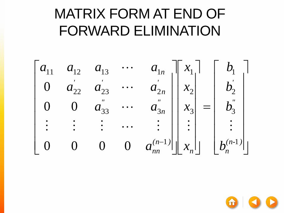
MATRIX FORM AT END OF
FORWARD ELIMINATION
)(n-
n
"
'
n
)(n
nn
"
n
"
'
n
''
n
b
b
b
b
x
x
x
x
a
aa
aaa
aaaa
1
3
2
1
3
2
1
1
333
22322
1131211
0000
00
0

BACK SUBSTITUTION
735.0
21.96
8.106
7.000
56.18.40
1525
3
2
1
x
x
x
Solve each equation starting from the last equation
Example of a system of 3 equations
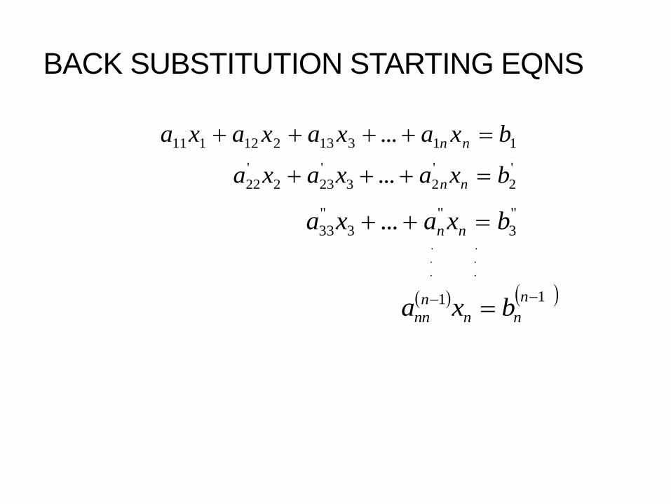
BACK SUBSTITUTION STARTING EQNS
'
2
'
23
'
232
'
22 ... bxaxaxa nn
"
3
"
3
"
33 ... bxaxa nn
11 n
nn
n
nn bxa
. .
. .
. .
11313212111 ... bxaxaxaxa nn
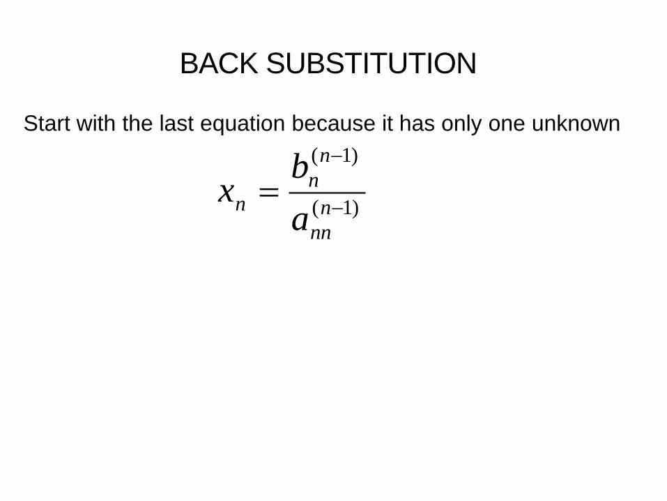
Start with the last equation because it has only one unknown
)1(
)1(
n
nn
n
n
na
bx
BACK SUBSTITUTION

1,...,1for...
1
1
,2
1
2,1
1
1,
1
nia
xaxaxabx
i
ii
n
i
nii
i
iii
i
ii
i
i
i
1,...,1for1
1
11
nia
xab
xi
ii
n
ijj
i
ij
i
i
i
)1(
)1(
n
nn
n
n
na
bx
BACK SUBSTITUTION

FORWARD ELIMINATION
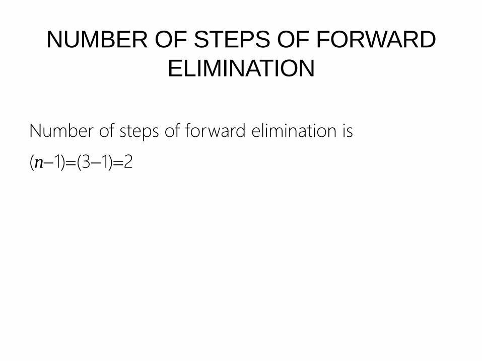
NUMBER OF STEPS OF FORWARD
ELIMINATION
Number of steps of forward elimination is
(n1)(31)2
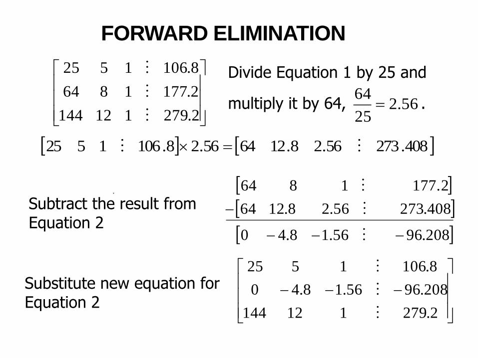
Divide Equation 1 by 25 and
multiply it by 64, .
.
408.27356.28.126456.28.1061525
208.96 56.18.4 0
408.273 56.2 8.1264
177.2 1 8 64
2.279112144
2.1771864
8.1061525
2.279112144
208.9656.18.40
8.1061525
56.225
64
Subtract the result from Equation 2
Substitute new equation for Equation 2
FORWARD ELIMINATION

FORWARD ELIMINATION: STEP 1 (CONT.)
.
168.61576.58.2814476.58.1061525
2.279112144
208.9656.18.40
8.1061525
968.335 76.48.16 0
168.615 76.5 8.28 144
279.2 1 12 144
968.33576.48.160
208.9656.18.40
8.1061525
Divide Equation 1 by 25 and
multiply it by 144, .76.525
144
Subtract the result from Equation 3
Substitute new equation for Equation 3
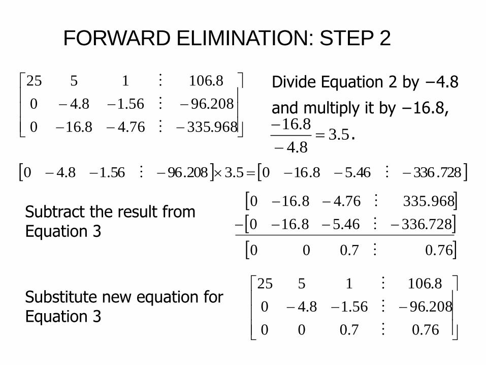
FORWARD ELIMINATION: STEP 2
728.33646.58.1605.3208.9656.18.40
968.33576.48.160
208.9656.18.40
8.1061525
.760 7.0 0 0
728.33646.516.80
335.968 76.416.80
76.07.000
208.9656.18.40
8.1061525
Divide Equation 2 by −4.8
and multiply it by −16.8,
.5.38.4
8.16
Subtract the result from Equation 3
Substitute new equation for Equation 3
BACK SUBSTITUTION

BACK SUBSTITUTION
76.0
208.96
8.106
7.000
56.18.40
1525
7.07.000
2.9656.18.40
8.1061525
3
2
1
a
a
a
08571.1
7.0
76.0
76.07.0
3
3
3
a
a
a
Solving for a3

BACK SUBSTITUTION (CONT.)
Solving for a2
690519.
4.8
1.085711.5696.208
8.4
56.1208.96
208.9656.18.4
2
2
32
32
a
a
aa
aa
76.0
208.96
8.106
7.000
56.18.40
1525
3
2
1
a
a
a
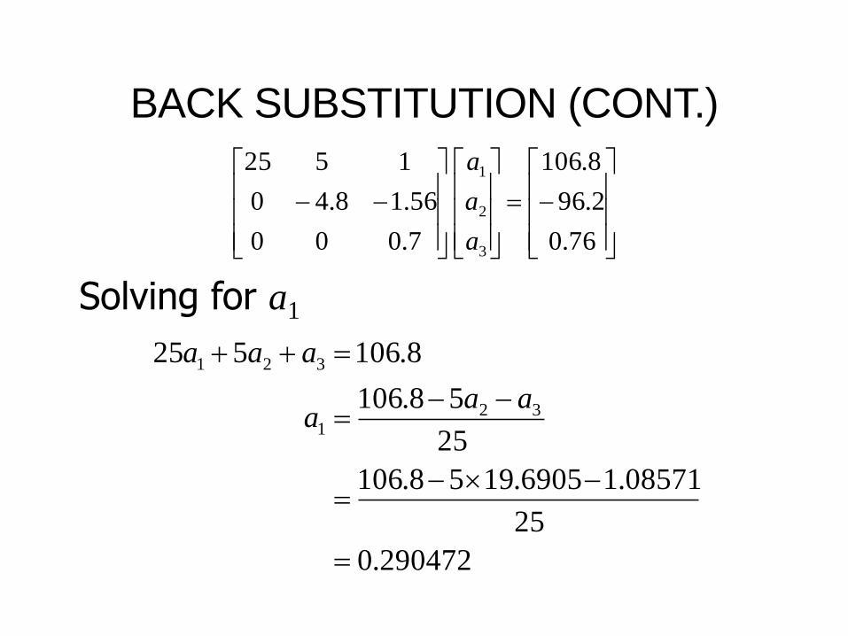
BACK SUBSTITUTION (CONT.)
Solving for a1
290472.0
25
08571.16905.1958.106
25
58.106
8.106525
321
321
aaa
aaa
76.0
2.96
8.106
7.000
56.18.40
1525
3
2
1
a
a
a

GAUSSIAN ELIMINATION
SOLUTION
2279
2177
8106
112144
1864
1525
3
2
1
.
.
.
a
a
a
08571.1
6905.19
290472.0
3
2
1
a
a
a

THANK YOU