
Trivial Pursuits?...2019/04/14 · Trivial Pursuits? ... Notes:
Upload
utrecht-universityCategory
view
586download
3description
University of Utrecht
MSc Thesis (Theoretical Physics)
Matrix Models of 2DString Theory in
Non–trivial Backgrounds
Arnaud Koetsier
Supervisors: Prof. G. ’t Hooft and Dr. S. Alexandrov

1/31
Overview of Talk
1. Introduction — the partition function
2. Critical strings in background fields
3. Noncritical strings and Liouville gravity
4. Matrix models and discretised surfaces
5. Matrix quantum mechanics (MQM)
6. MQM in the chiral representation
7. Conclusion and outlook

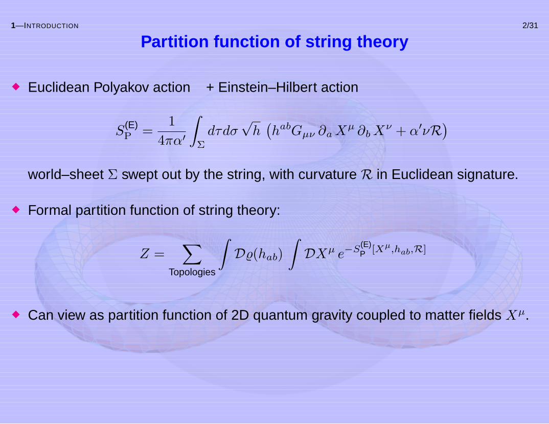
1—INTRODUCTION 2/31
Partition function of string theory
Euclidean Polyakov action + Einstein–Hilbert action
S(E)P =
14πα′
∫Σ
dτdσ√h(habGµν ∂aX
µ ∂bXν + α′νR
)world–sheet Σ swept out by the string, with curvature R in Euclidean signature.
Formal partition function of string theory:
Z =∑
Topologies
∫D%(hab)
∫DXµ e−S
(E)P [Xµ,hab,R]
Can view as partition function of 2D quantum gravity coupled to matter fields Xµ.
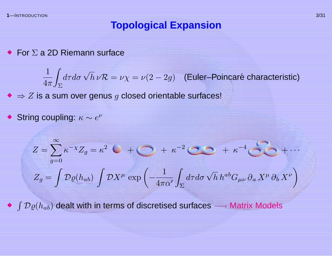
1—INTRODUCTION 3/31
Topological Expansion
For Σ a 2D Riemann surface
14π
∫Σ
dτdσ√h νR = νχ = ν(2− 2g) (Euler–Poincare characteristic)
⇒ Z is a sum over genus g closed orientable surfaces!
String coupling: κ ∼ eν
Z =∞∑
g=0
κ−χZg = κ2 + + κ−2 + κ−4 + · · ·
Zg =∫D%(hab)
∫DXµ exp
(− 1
4πα′
∫Σ
dτdσ√hhabGµν ∂aX
µ ∂bXν
)∫D%(hab) dealt with in terms of discretised surfaces −→ Matrix Models
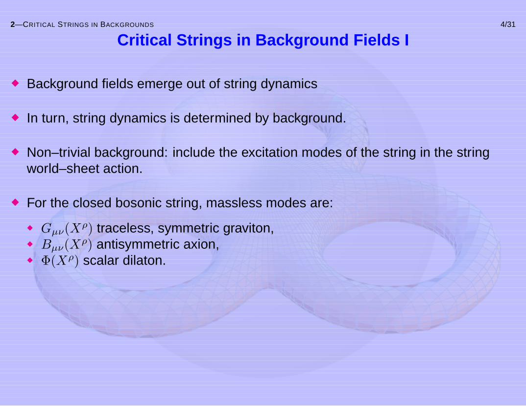
2—CRITICAL STRINGS IN BACKGROUNDS 4/31
Critical Strings in Background Fields I
Background fields emerge out of string dynamics
In turn, string dynamics is determined by background.
Non–trivial background: include the excitation modes of the string in the stringworld–sheet action.
For the closed bosonic string, massless modes are:
Gµν(Xρ) traceless, symmetric graviton,Bµν(Xρ) antisymmetric axion,Φ(Xρ) scalar dilaton.

2—CRITICAL STRINGS IN BACKGROUNDS 5/31
Critical Strings in Background Fields II
Adding those fields to the action, we get a sigma model in D dimensions
Sσ =1
4πα′
∫d2σ√h[ (habGµν(X) + iεabBµν(X)
)∂aX
µ ∂bXν
+α′RΦ(X)]
NB: Coupling constants on the world–sheet become fields in the target space. e.g.ν → Φ(X).
Gµν, Bµν and Φ so far unconstrained.
Each “running coupling” (target–space field) has a renormalization groupβ–function
=⇒ Theory should possess conformal invariance =⇒ β–functions vanish

2—CRITICAL STRINGS IN BACKGROUNDS 6/31
β–functions
To zeroth order in α′
βGµν = Rµν + 2DµDνΦ−
14HµσρHν
σρ = 0,
βBµν = DρHµν
ρ − 2HµνρDρΦ = 0,
βΦ =1α′D − 2648π2
+1
16π2
[4(DµΦ)2 − 4DµD
µΦ−R+112HµνρH
µνρ
]= 0,
Hµνρ = ∂µBνρ + ∂ρBµν + ∂ν Bρµ
Critical string theory:
Gµν = ηµν, Bµν = 0, Φ = ν ⇒ D = 26
Solution of interest: Linear dilaton background
Gµν = ηµν, Bµν = 0, Φ = lµXµ.

2—CRITICAL STRINGS IN BACKGROUNDS 7/31
Problem: Divergent String Coupling
Linear dilaton background in present form leads to a divergent string coupling.
String couplingκ ∝ eν = eΦ(Xρ) = elµXµ
=⇒ For some Xµ, coupling diverges!
Solution: add a potential to the sigma model
Scosmoσ =
14πα′
∫d2σ√hT (Xµ)
2—CRITICAL STRINGS IN BACKGROUNDS 8/31
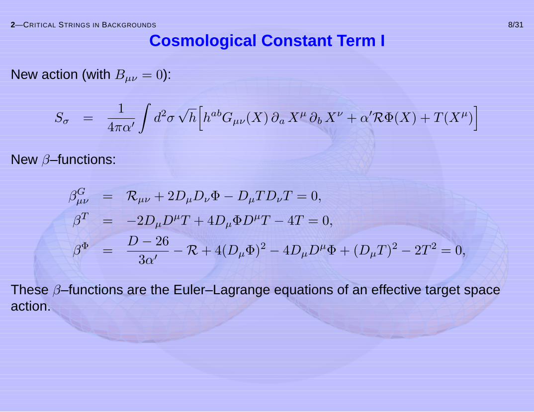
Cosmological Constant Term I
New action (with Bµν = 0):
Sσ =1
4πα′
∫d2σ√h[habGµν(X) ∂aX
µ ∂bXν + α′RΦ(X) + T (Xµ)
]New β–functions:
βGµν = Rµν + 2DµDνΦ−DµTDνT = 0,
βT = −2DµDµT + 4DµΦDµT − 4T = 0,
βΦ =D − 26
3α′−R+ 4(DµΦ)2 − 4DµD
µΦ + (DµT )2 − 2T 2 = 0,
These β–functions are the Euler–Lagrange equations of an effective target spaceaction.
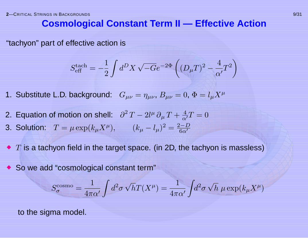
2—CRITICAL STRINGS IN BACKGROUNDS 9/31
Cosmological Constant Term II — Effective Action
“tachyon” part of effective action is
Stacheff = −1
2
∫dDX
√−Ge−2Φ
((DµT )2 − 4
α′T 2
)
1. Substitute L.D. background: Gµν = ηµν, Bµν = 0, Φ = lµXµ
2. Equation of motion on shell: ∂2 T − 2lµ ∂µ T + 4α′T = 0
3. Solution: T = µ exp(kµXµ), (kµ − lµ)2 = 2−D
6α′
T is a tachyon field in the target space. (in 2D, the tachyon is massless)
So we add “cosmological constant term”
Scosmoσ =
14πα′
∫d2σ√hT (Xµ) =
14πα′
∫d2σ√h µ exp(kµX
µ)
to the sigma model.
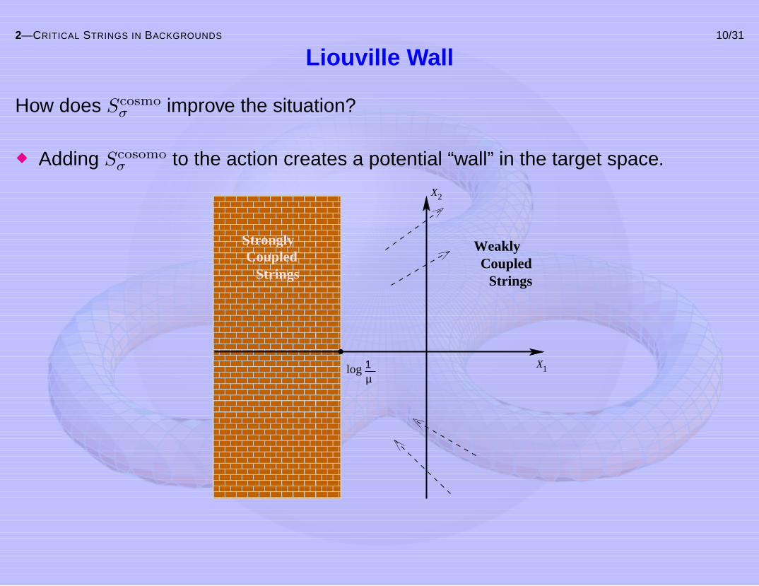
2—CRITICAL STRINGS IN BACKGROUNDS 10/31
Liouville Wall
How does Scosmoσ improve the situation?
Adding Scosomoσ to the action creates a potential “wall” in the target space.
1
2
CoupledWeakly
Strongly
StringsCoupled
X
X
µ1log
Strings

2—CRITICAL STRINGS IN BACKGROUNDS 11/31
Critical string theory with L.D. background— Summary —
Action for critical string theory in D dimensions, in a linear dilaton background:
SLDσ =
14πα′
∫d2σ√h[hab ∂aX
µ ∂bXµ + α′RlµXµ + µekµXµ]
(kµ − lµ)2 =2−D6α′
This is an exact, well defined conformal field theory.
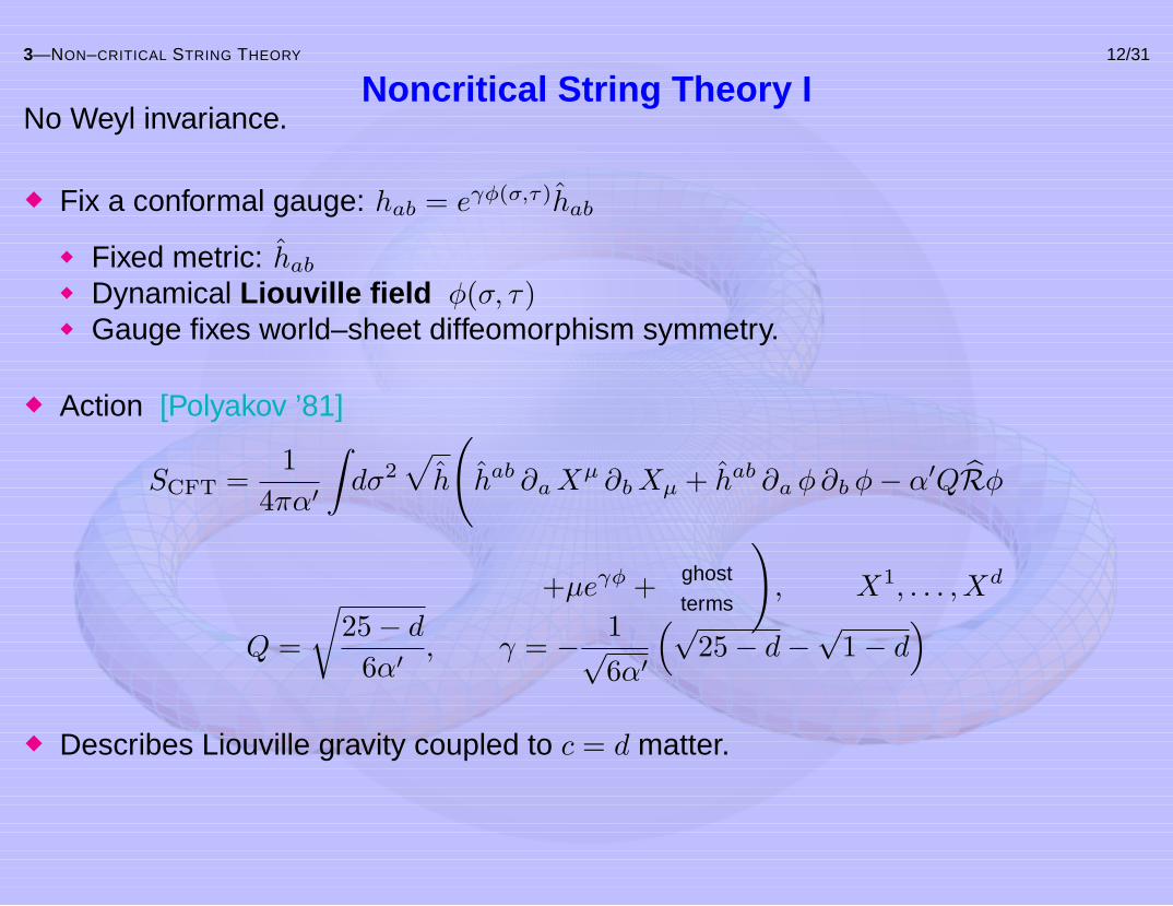
3—NON–CRITICAL STRING THEORY 12/31
Noncritical String Theory INo Weyl invariance.
Fix a conformal gauge: hab = eγφ(σ,τ)hab
Fixed metric: hab
Dynamical Liouville field φ(σ, τ)Gauge fixes world–sheet diffeomorphism symmetry.
Action [Polyakov ’81]
SCFT =1
4πα′
∫dσ2
√h
(hab ∂aX
µ ∂bXµ + hab ∂a φ∂b φ− α′QRφ
+µeγφ + ghost
terms
), X1, . . . , Xd
Q =
√25− d
6α′, γ = − 1√
6α′
(√25− d−
√1− d
)Describes Liouville gravity coupled to c = d matter.

3—NON–CRITICAL STRING THEORY 13/31
Non–critical ↔ Critical String Theory
Now, compare:
SCFT =1
4πα′
∫dσ2
√h(hab ∂aX
µ ∂bXµ + hab ∂a φ∂b φ
− α′QRφ + µeγφ), X1, . . . , Xd
SLDσ =
14πα′
∫d2σ√h(hab ∂aX
µ ∂bXµ
+ α′RlµXµ + µekµXµ), X1, . . . , XD
Make the following associations:
D = d+ 1; XD = φ, lµ =
0; µ 6= D−Q, µ = D
; kµ =
0, µ 6= Dγ, µ = D
Then, SCFT = SLDσ

3—NON–CRITICAL STRING THEORY 14/31
Non–critical ↔ Critical String Theory— Summary —
d Dimensional noncritical string theory=
d+ 1 Dimensional critical string theory in L.D. background.
2D bosonic string theory in a linear dilaton background = Liouville gravity coupledto c = 1 matter, or non–critical string theory in 1 dimension (α′ = 1):
SCFT =14π
∫d2σ√h(hab ∂aX ∂bX + hab ∂a φ∂b φ− 2Rφ+ µe−2φ
)
3—NON–CRITICAL STRING THEORY 15/31
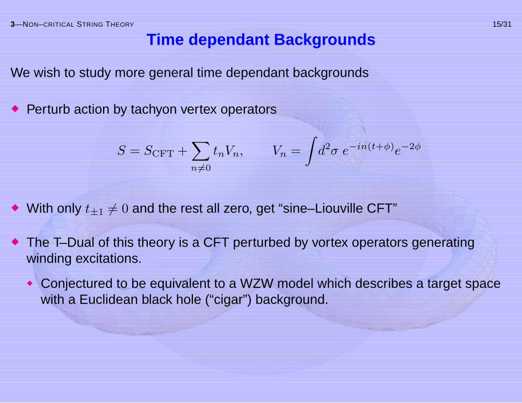
Time dependant Backgrounds
We wish to study more general time dependant backgrounds
Perturb action by tachyon vertex operators
S = SCFT +∑n 6=0
tnVn, Vn =∫d2σ e−in(t+φ)e−2φ
With only t±1 6= 0 and the rest all zero, get “sine–Liouville CFT”
The T–Dual of this theory is a CFT perturbed by vortex operators generatingwinding excitations.
Conjectured to be equivalent to a WZW model which describes a target spacewith a Euclidean black hole (“cigar”) background.

3—NON–CRITICAL STRING THEORY 16/31
Cigar Manifold
Asymptotically, the metric looks like
ds2 = −(1− e−2Qr
)dt2 +
11− e−2Qr
dr2, Φ = %0 −Qr.
Curvature is RG = 4Q2e−2Qr. Performing analytic continuation to Euclidean timet 7→ iθ, get the Euclidean cigar:

3—MATRIX MODELS 17/31
Matrix Models — Definition
A matrix model consists of
Symmetry group GEnsemble of N ×N matrices M invariant under GProbability law (partition function)
Z =∫dM exp [−N Tr V (M)] , V (M) =
∑k>0
gk
kMk
We are interested in unitary matrix ensembles: G = U(N), M hermitian.
As in QFT, we can write down a perturbation expansion in terms of Feynmandiagrams from the partition function (N ∼ −1).
3—MATRIX MODELS 18/31
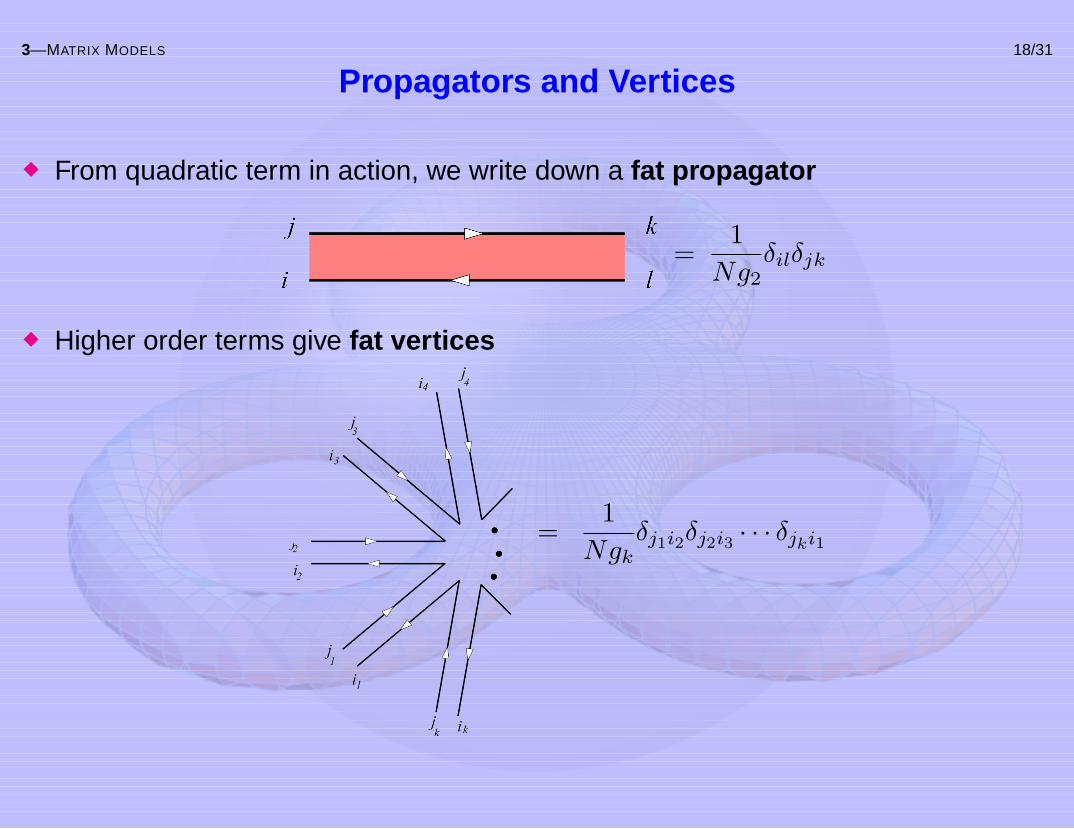
Propagators and Vertices
From quadratic term in action, we write down a fat propagator
=1
Ng2δilδjk
Higher order terms give fat vertices
=1
Ngkδj1i2δj2i3 · · · δjki1

3—MATRIX MODELS 19/31
Discretised SurfacesDuality: Feynman graph network←→ Discretised surface
Discretised surface
Dual Propogator
3—MATRIX MODELS 20/31
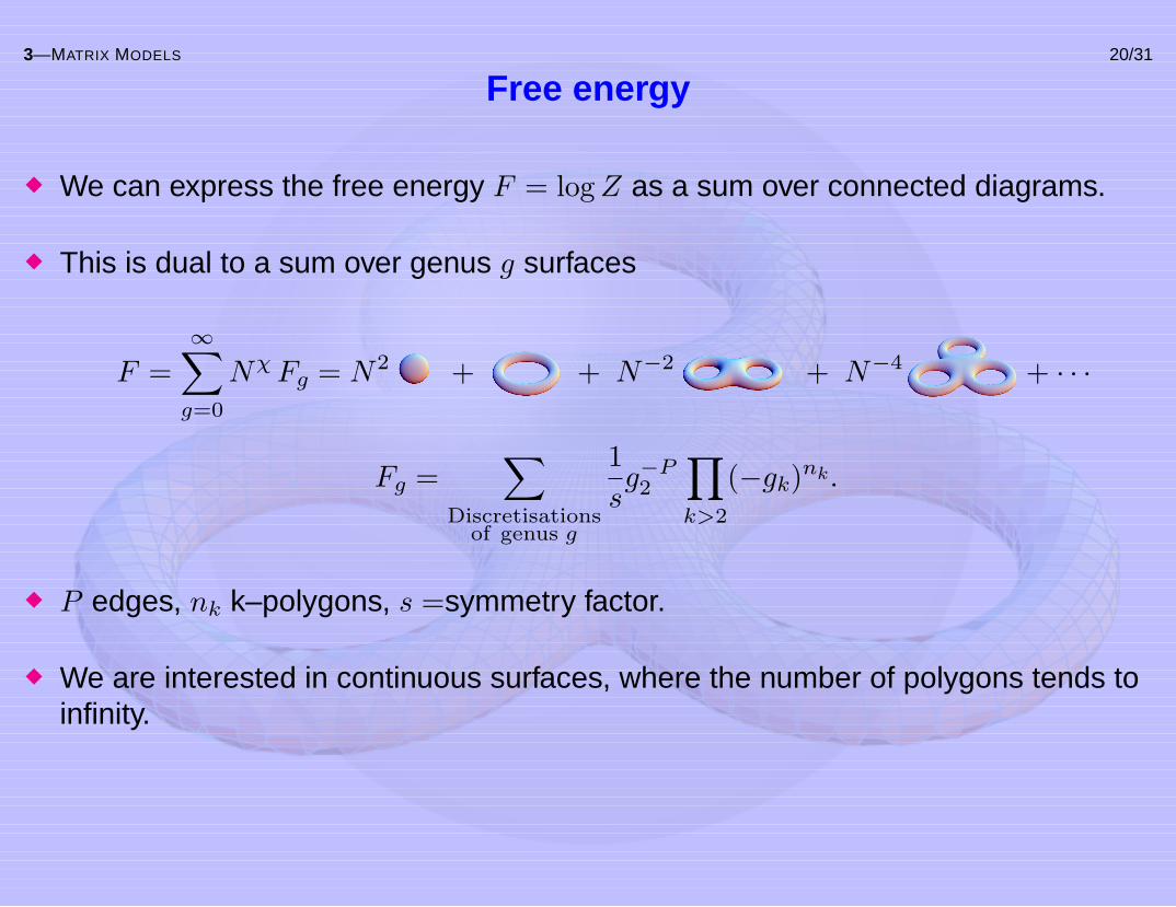
Free energy
We can express the free energy F = logZ as a sum over connected diagrams.
This is dual to a sum over genus g surfaces
F =∞∑
g=0
NχFg = N2 + + N−2 + N−4 + · · ·
Fg =∑
Discretisationsof genus g
1sg−P2
∏k>2
(−gk)nk.
P edges, nk k–polygons, s =symmetry factor.
We are interested in continuous surfaces, where the number of polygons tends toinfinity.

3—MATRIX MODELS 21/31
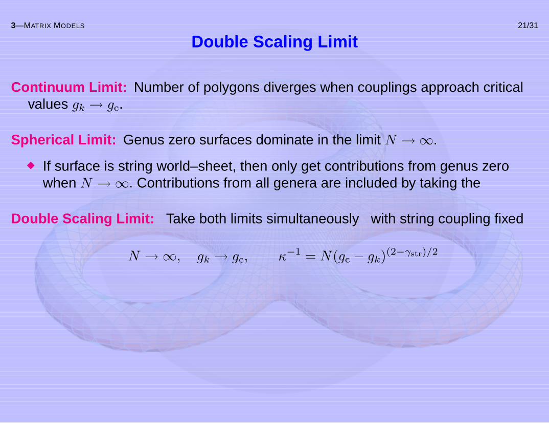
Double Scaling Limit
Continuum Limit: Number of polygons diverges when couplings approach criticalvalues gk → gc.
Spherical Limit: Genus zero surfaces dominate in the limit N →∞.
If surface is string world–sheet, then only get contributions from genus zerowhen N →∞. Contributions from all genera are included by taking the
Double Scaling Limit: Take both limits simultaneously with string coupling fixed
N →∞, gk → gc, κ−1 = N(gc − gk)(2−γstr)/2
4—MQM 22/31
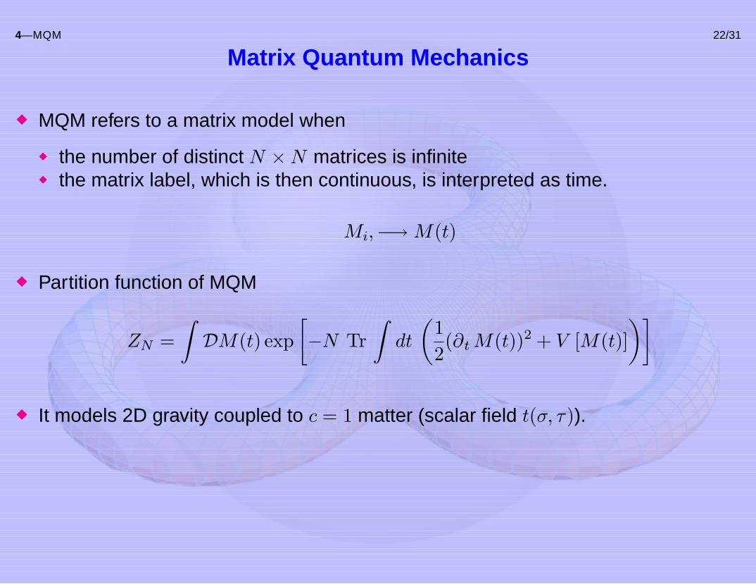
Matrix Quantum Mechanics
MQM refers to a matrix model when
the number of distinct N ×N matrices is infinitethe matrix label, which is then continuous, is interpreted as time.
Mi,−→M(t)
Partition function of MQM
ZN =∫DM(t) exp
[−N Tr
∫dt
(12(∂tM(t))2 + V [M(t)]
)]
It models 2D gravity coupled to c = 1 matter (scalar field t(σ, τ)).

4—MQM 23/31
Hamiltonian Analysis
Diagonalize the matrices
M(t) = Ω†(t)x(t)Ω(t), x(t) = diagx1(t), . . . , xN(t), ,Ω†(t)Ω(t) = 1
Quantum Hamiltonian of the system:
HMQM =N∑
i=1
(−2
2∆(x)∂2
∂ x2i
∆(x) + V (xi)
)+
12
∑i<j
Π2ij + Π2
ij
(xi − xj)2.
Write partition function as
ZN = Tr e−1T bHMQM, T → ∞
In this limit, only ground state contributes to the free energy
F = −E0
4—MQM 24/31
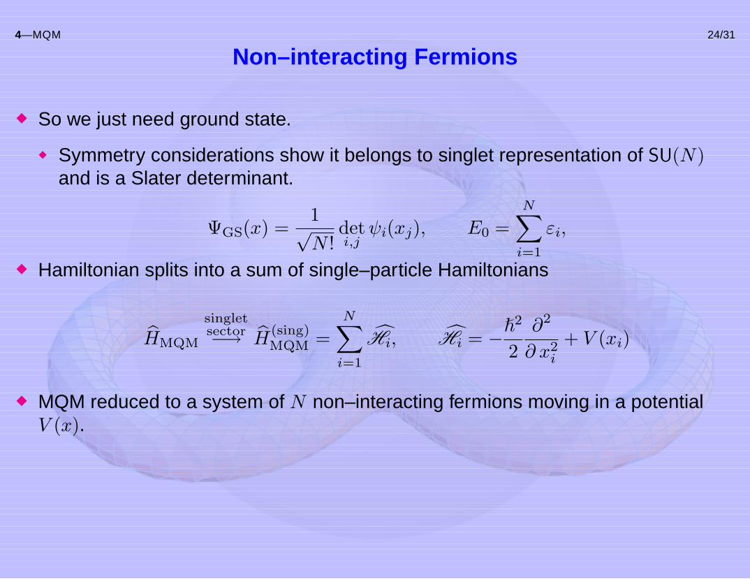
Non–interacting Fermions
So we just need ground state.
Symmetry considerations show it belongs to singlet representation of SU(N)and is a Slater determinant.
ΨGS(x) =1√N !
deti,j
ψi(xj), E0 =N∑
i=1
εi,
Hamiltonian splits into a sum of single–particle Hamiltonians
HMQM
singletsector−→ H
(sing)MQM =
N∑i=1
Hi, Hi = −2
2∂2
∂ x2i
+ V (xi)
MQM reduced to a system of N non–interacting fermions moving in a potentialV (x).
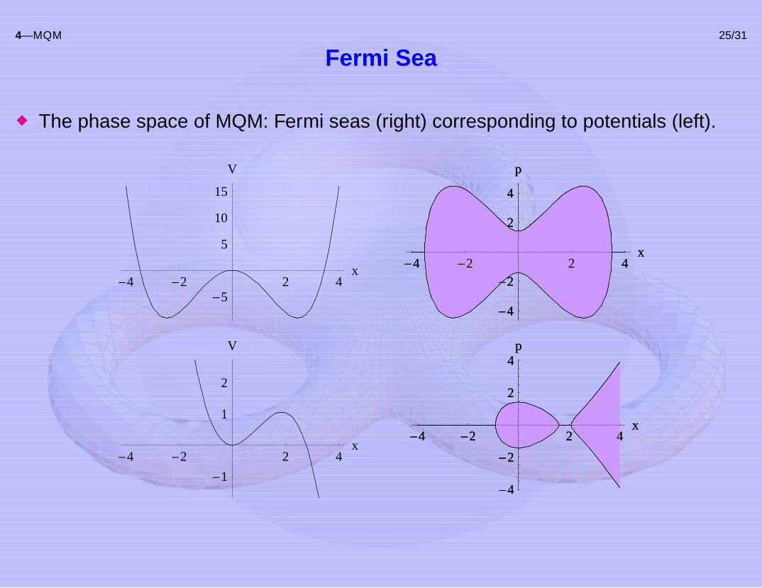
4—MQM 25/31
Fermi Sea
The phase space of MQM: Fermi seas (right) corresponding to potentials (left).
-4 -2 2 4x
-1
1
2
V
-4 -2 2 4x
-4
-2
2
4p
-4 -2 2 4x
-4
-2
2
4p
-4 -2 2 4x
-5
5
10
15
V
-4 -2 2 4x
-4
-2
2
4
p
-4 -2 2 4x
-4
-2
2
4
p
4—MQM 26/31
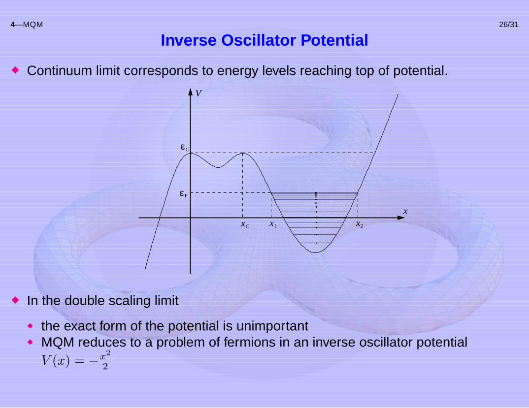
Inverse Oscillator Potential
Continuum limit corresponds to energy levels reaching top of potential.
V
Cε
x xx
εF
C 1 2
x
In the double scaling limit
the exact form of the potential is unimportantMQM reduces to a problem of fermions in an inverse oscillator potentialV (x) = −x2
2
5—MQM IN THE CHIRAL REPRESENTATION 27/31
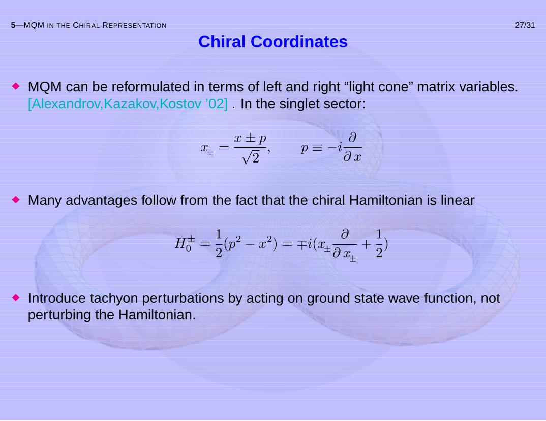
Chiral Coordinates
MQM can be reformulated in terms of left and right “light cone” matrix variables.[Alexandrov,Kazakov,Kostov ’02] . In the singlet sector:
x± =x± p√
2, p ≡ −i ∂
∂ x
Many advantages follow from the fact that the chiral Hamiltonian is linear
H±0 =
12(p2 − x2) = ∓i(x±
∂
∂ x±+
12)
Introduce tachyon perturbations by acting on ground state wave function, notperturbing the Hamiltonian.
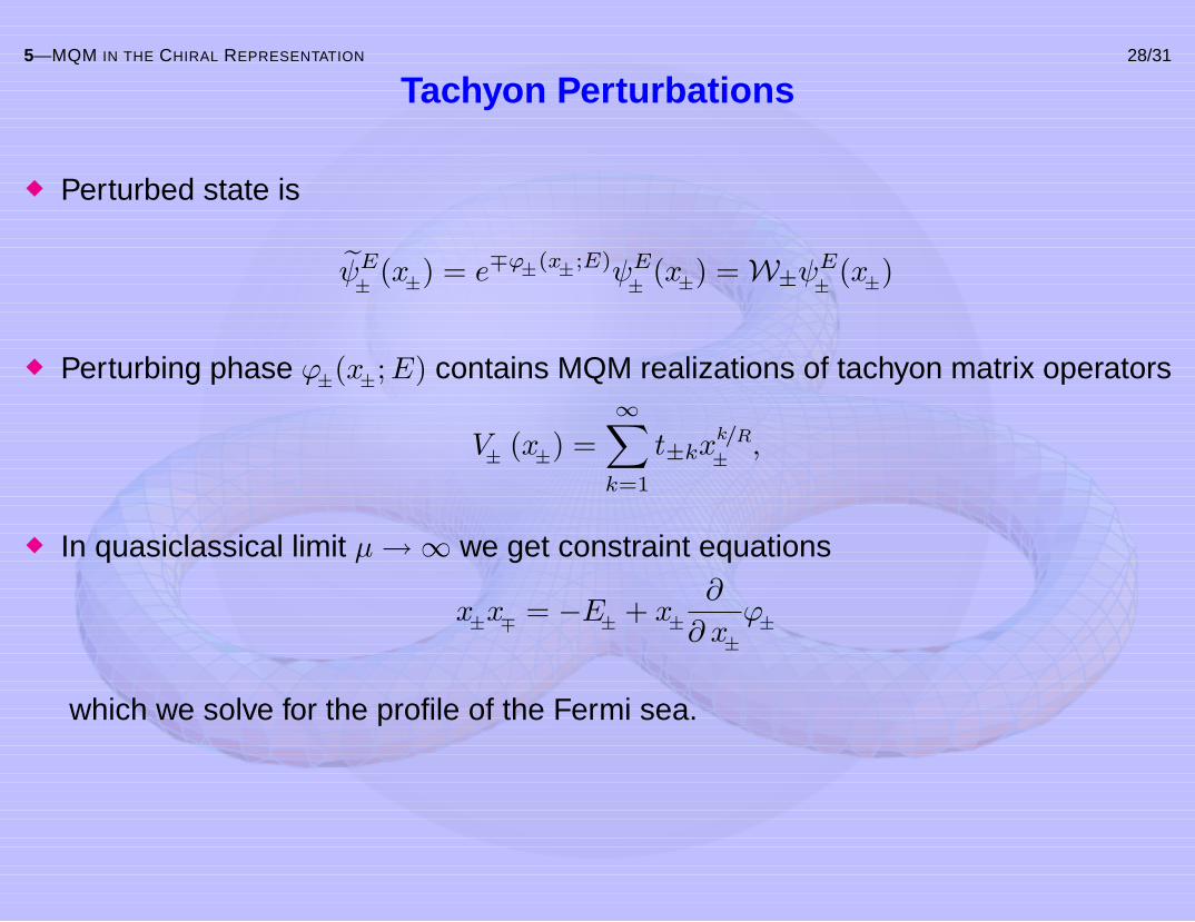
5—MQM IN THE CHIRAL REPRESENTATION 28/31
Tachyon Perturbations
Perturbed state is
ψE± (x±) = e∓ϕ±(x±;E)ψE
± (x±) =W±ψE± (x±)
Perturbing phase ϕ±(x±;E) contains MQM realizations of tachyon matrix operators
V± (x±) =∞∑
k=1
t±kxk/R
± ,
In quasiclassical limit µ→∞ we get constraint equations
x±x∓ = −E± + x±∂
∂ x±ϕ±
which we solve for the profile of the Fermi sea.
5—MQM IN THE CHIRAL REPRESENTATION 29/31
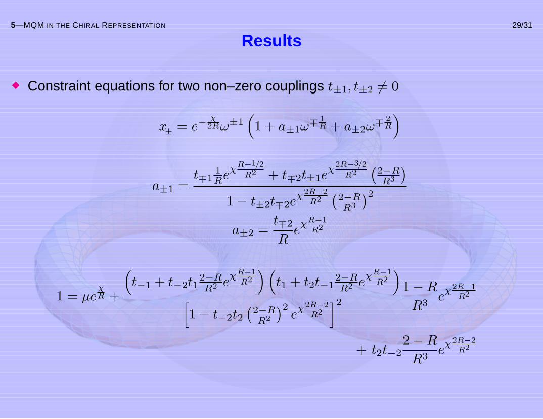
Results
Constraint equations for two non–zero couplings t±1, t±2 6= 0
x± = e−χ2Rω±1
(1 + a±1ω
∓ 1R + a±2ω
∓ 2R
)
a±1 =t∓1
1Re
χR−1/2
R2 + t∓2t±1eχ
2R−3/2
R2(2−RR3
)1− t±2t∓2e
χ2R−2R2(2−RR3
)2a±2 =
t∓2
Re
χR−1R2
1 = µeχR +
(t−1 + t−2t1
2−RR2 e
χR−1R2
)(t1 + t2t−1
2−RR2 e
χR−1R2
)[1− t−2t2
(2−RR2
)2e
χ2R−2R2
]2 1−RR3
eχ2R−1
R2
+ t2t−22−RR3
eχ2R−2
R2
5—MQM IN THE CHIRAL REPRESENTATION 30/31
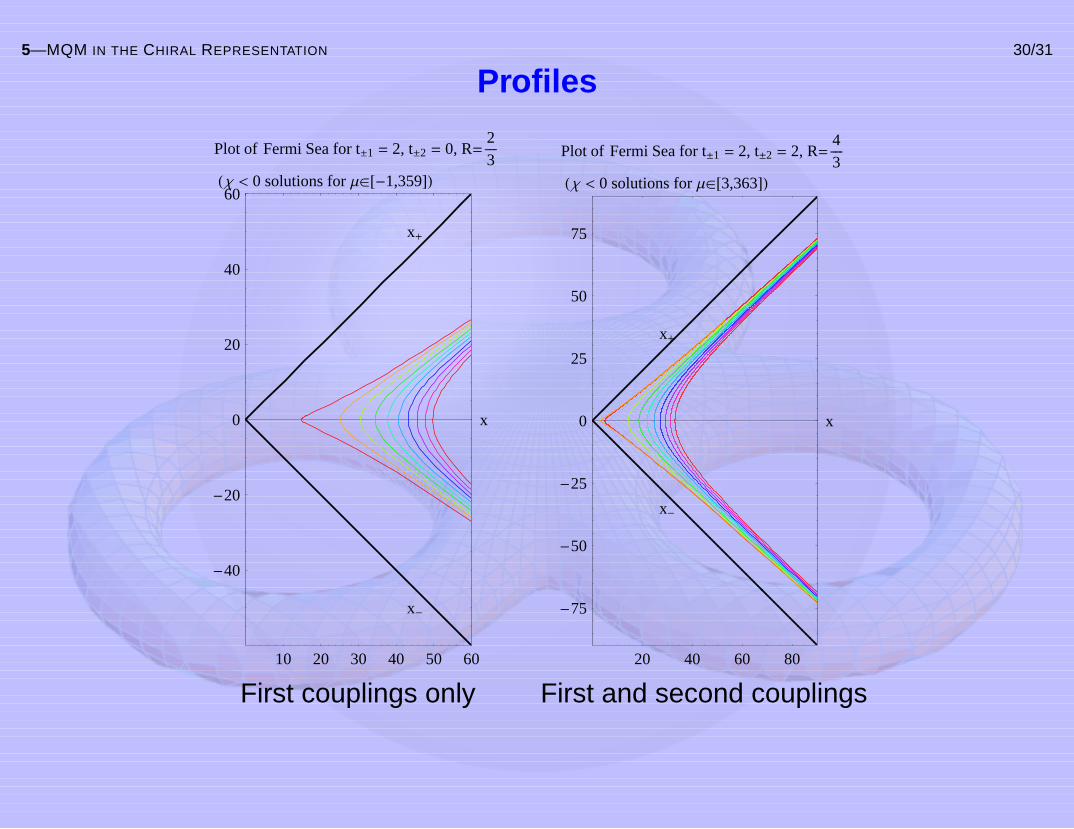
Profiles
10 20 30 40 50 60
-40
-20
0
20
40
60
x
Plot of Fermi Sea for t±1 = 2, t±2 = 0, R=23
HΧ < 0 solutions for ΜÎ@-1,359DL
x+
x-
20 40 60 80
-75
-50
-25
0
25
50
75
x
Plot of Fermi Sea for t±1 = 2, t±2 = 2, R=43
HΧ < 0 solutions for ΜÎ@3,363DL
x+
x-
First couplings only First and second couplings
5—MQM IN THE CHIRAL REPRESENTATION 31/31
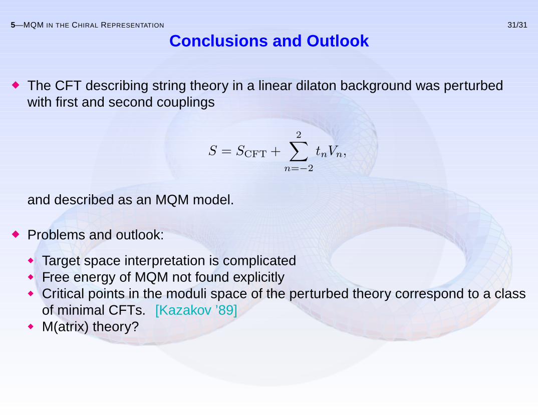
Conclusions and Outlook
The CFT describing string theory in a linear dilaton background was perturbedwith first and second couplings
S = SCFT +2∑
n=−2
tnVn,
and described as an MQM model.
Problems and outlook:
Target space interpretation is complicatedFree energy of MQM not found explicitlyCritical points in the moduli space of the perturbed theory correspond to a classof minimal CFTs. [Kazakov ’89]M(atrix) theory?