Matrix Factorization In Recommender Systems

Yong Zheng, PhDc

Center for Web Intelligence, DePaul University, USA

March 4, 2015

Matrix Factorization In Recommender Systems

• Background: Recommender Systems (RS)

• Evolution of Matrix Factorization (MF) in RS PCA SVD Basic MF Extended MF

• Dimension Reduction: PCA & SVD Other Applications: image processing, etc

• An Example: MF in Recommender Systems Basic MF and Extended MF

Table of Contents

1. Recommender System (RS)

• Definition: RS is a system able to provide or suggest items to the end users.


• Function: Alleviate information overload problems

Recommendation

1. Recommender System (RS) • Function: Alleviate information overload problems

Social RS (Twitter) Tagging RS (Flickr)


• Task-1: Rating Predictions

• Task-2: Top-N Recommendation

Provide a short list of recommendations; For example, top-5 twitter users, top-10 news;

User HarryPotter Batman Spiderman

U1 5 3 4

U2 ? 2 4

U3 4 2 ?

1. Recommender System (RS) • Evolution of Recommendation algorithms





Table of Contents

2. Matrix Factorization In RS

• Why we need MF in RS?

The very beginning: dimension reduction Amazon.com: thousands of users and items; Netflix.com: thousands of users and movies; How large the rating matrix it is ?????????? Computational costs high !!!


• Netflix Prize ($1 Million Contest), 2006-2009


• Netflix Prize ($1 Million Contest), 2006-2009

How about using BigData mining, such as MapReduce? 2003 - Google launches project Nutch 2004 - Google releases papers with MapReduce 2005 - Nutch began to use GFS and MapReduce 2006 - Yahoo! created Hadoop based on GFS & MapReduce 2007 - Yahoo started using Hadoop on a 1000 node cluster 2008 - Apache took over Hadoop 2009 - Hadoop was successfully process large-scale data 2011 - Hadoop releases version 1.0


• Evolution of Matrix Factorization (MF) in RS

Dimension Reduction Techniques: PCA & SVD

SVD-Based Matrix Factorization (SVD)

Basic Matrix Factorization

Extended Matrix Factorization

Modern Stage

Early Stage





Table of Contents

3. Dimension Reduction

• Why we need dimension reduction?

The curse of dimensionality: various problems that arise when analyzing and organizing data in high-dimensional spaces that do not occur in low-dimensional settings such as 2D or 3D spaces.

• Applications

Information Retrieval: Web documents, where the dimensionality is the vocabulary of words Recommender System: Large scale of rating matrix Social Networks: Facebook graph, where the dimensionality is the number of users Biology: Gene Expression Image Processing: Facial recognition


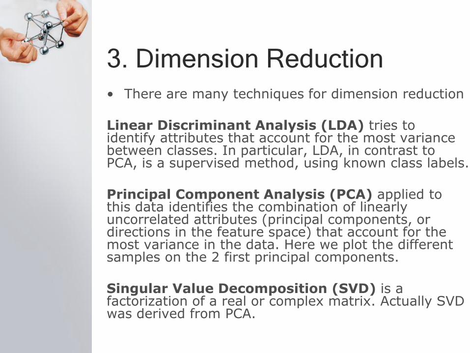
• There are many techniques for dimension reduction

Linear Discriminant Analysis (LDA) tries to identify attributes that account for the most variance between classes. In particular, LDA, in contrast to PCA, is a supervised method, using known class labels.

Principal Component Analysis (PCA) applied to this data identifies the combination of linearly uncorrelated attributes (principal components, or directions in the feature space) that account for the most variance in the data. Here we plot the different samples on the 2 first principal components. Singular Value Decomposition (SVD) is a factorization of a real or complex matrix. Actually SVD was derived from PCA.

3. Dimension Reduction • Brief History

Principal Component Analysis (PCA) - Draw a plane closest to data points (Pearson, 1901) - Retain most variance of the data (Hotelling, 1933) Singular Value Decomposition (SVD) - Low-rank approximation (Eckart-Young, 1936) - Practical applications or Efficient Computations

(Golub-Kahan, 1965)

Matrix Factorization In Recommender Systems - “Factorization Meets the Neighborhood: a Multifaceted.

Collaborative Filtering Model”，by Yehuda Koren, ACM KDD 2008 (formally reach an agreement by this paper)

3. Dimension Reduction Principal Component Analysis (PCA) Assume we have a data with multiple features 1). Try to find principle components – each component is a combination of the linearly uncorrelated attributes/features; 2). PCA allows to obtain an ordered list of those components that account for the largest amount of the variance from the data; 3). The amount of variance captured by the first component is larger than the amount of variance on the second component, and so on. 4). Then, we can reduce the dimensionality by ignoring the components with smaller contributions to the variance.


Principal Component Analysis (PCA) How to obtain those principal components? The basic principle or assumption in PCA is: The eigenvector of a covariance matrix equal to a principal component, because the eigenvector with the largest eigenvalue is the direction along which the data set has the maximum variance. Each eigenvector is associated with a eigenvalue; Eigenvalue tells how much the variance is; Eigenvector tells the direction of the variation; The next step: how to get the covariance matrix and how to calculate the eigenvectors/eigenvalues?


Principal Component Analysis (PCA) Step by steps Assume a data with 3 dimensions Step1: Center the data by subtracting the mean of each column

Mean(X) = 4.35

Mean (Y) = 4.292

Mean (Z) = 3.19

For example,

X11 = 2.5

Update:

X11 = 2.5-4.35 = -1.85

Original Data Transformed Data


Principal Component Analysis (PCA) Step2: Compute covariance matrix based on the transformed data

Matlab function: cov (Matrix)


Principal Component Analysis (PCA) Step3: Calculate eigenvectors & eigenvalues from covariance matrix

Matlab function:

[V,D] = eig (Covariance Matrix)

V = eigenvectors (each column)

D = eigenvalues (in the diagonal line) For example, 2.9155 correspond to vector <0.3603, -0.3863, 0.8491>

Each eigenvector is considered as a principle component.


Principal Component Analysis (PCA) Step4: Order the eigenvalues from largest to smallest, where the eigenvectors will also be re-ordered; and then we can select the top-K one; for example, we set K=2

K=2, it indicates that we will

reduce the dimensions to be

2. The last second columns

are extracted to have an

EigenMatrix


Principal Component Analysis (PCA) Step5: Project the original data to those eigenvectors to formulate the new data matrix

Original data, D, 10x3 Transformed data, TD, 10x3 EigenMatrix, EM, 3X2

FinalData (10xk) = TD (10x3) x EM (3xk), here k = 2



Original data, D, 10x3 Final Data, FD, 10x2

FinalData (10xk) = TD (10x3) x EM (3xk), here k = 2

After PCA



PCA finds a linear projection of high dimensional data into a lower dimensional subspace.

The idea of Projection Visualization of PCA


Principal Component Analysis (PCA) PCA reduces the dimensionality (the number of features) of a data set by maintaining as much variance as possible. Another example: Gene Expression

The original expression by 3 genres is projected to two new dimensions, Such

two-dimensional visualization of the samples allow us to draw qualitative conclusions about

the separability of experimental conditions (marked by different colors).


Singular Value Decomposition (SVD) • SVD is another approach used for dimension reduction; • Specifically, it is developed for Matrix Decomposition; • SVD actually is another way to do PCA; • The application of SVD to the domain of recommender

systems was boosted by the Netflix Prize Contest

Winner: BELLKOR’S PRAGMATIC CHAOS


Singular Value Decomposition (SVD) Any N × d matrix X can be decomposed in this way: r is the rank of matrix X, = the size of the largest

collection of linearly independent columns or rows in matrix X ;

U is a column-orthonormal N × r matrix; V is a column-orthonormal d × r matrix; ∑ is a diagonal r × r matrix, where the singular values

are sorted in descending order.

X U ∑ VT


Singular Value Decomposition (SVD) Any N × d matrix X can be decomposed in this way: Relations between PCA and SVD:

X U ∑ VT

In other words, V contains eigenvectors, and the ordered eigenvalues are present in ∑.


Singular Value Decomposition (SVD)


Singular Value Decomposition (SVD) Any N × d matrix X can be decomposed in this way: So, how to realize the dimension reduction in SVD? Simply, based on the computation above, SVD tries to find a matrix to approximate the original matrix X by reducing the value of r – only the selected eigenvectors corresponding to the top-K largest eigenvalues will be obtained; other dimension will be discarded.

X U ∑ VT


Singular Value Decomposition (SVD) So, how to realize the dimension reduction in SVD? SVD is an optimization algorithm. Assume original data matrix is X, and SVD process is to find an approximation

minimize the Frobenius norm over

all rank-k matrices ||X – D||F


References - Pearson, Karl. "Principal components analysis." The London,

Edinburgh, and Dublin Philosophical Magazine and Journal of Science 6.2 (1901): 559.

- De Lathauwer, L., et al. "Singular Value Decomposition." Proc. EUSIPCO-94, Edinburgh, Scotland, UK. Vol. 1. 1994.

- Wall, Michael E., Andreas Rechtsteiner, and Luis M. Rocha. "Singular value decomposition and principal component analysis." A practical approach to microarray data analysis. Springer US, 2003. 91-109.

- Sarwar, Badrul, et al. Application of dimensionality reduction in recommender system-a case study. No. TR-00-043. Minnesota Univ Minneapolis Dept of Computer Science, 2000.


Relevant Courses at CDM, DePaul University CSC 424 Advanced Data Analysis CSC 529 Advanced Data Mining CSC 478 Programming Data Mining Applications ECT 584 Web Data Mining for Business Intelligence





Table of Contents

4. MF in Recommender Systems

• Evolution of Matrix Factorization (MF) in RS

Dimension Reduction Techniques: PCA & SVD

SVD-Based Matrix Factorization (SVD)

Basic Matrix Factorization

Extended Matrix Factorization

Modern Stage

Early Stage


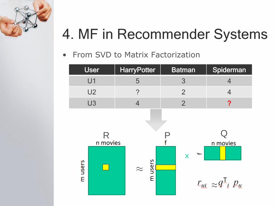
• From SVD to Matrix Factorization


U1 5 3 4

U2 ? 2 4

U3 4 2 ?



Rating Prediction function in SVD for Recommendation

C is a user, P is the item (e.g. movie)

We create two new matrices: and

They are considered as user and item matrices

We extract the corresponding row (by c) and column (by p) from

those matrices for computation purpose.




U1 5 3 4

U2 ? 2 4

U3 4 2 ?

R P Q


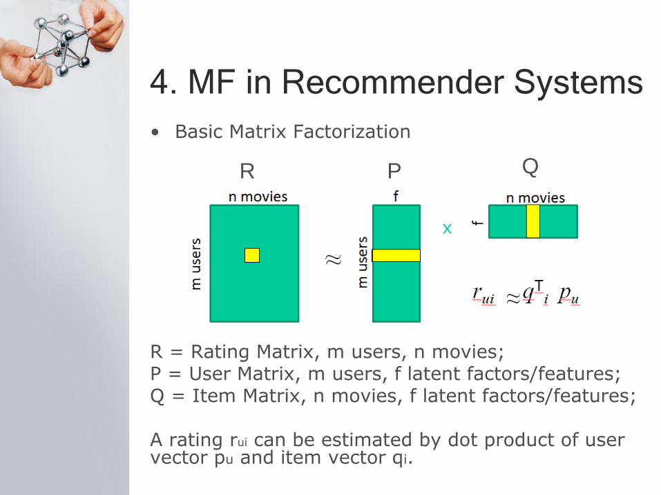
• Basic Matrix Factorization

R = Rating Matrix, m users, n movies; P = User Matrix, m users, f latent factors/features; Q = Item Matrix, n movies, f latent factors/features; A rating rui can be estimated by dot product of user vector pu and item vector qi.

R P Q



Interpretation: pu indicates how much user likes f latent factors; qi means how much one item obtains f latent factors; The dot product indicates how much user likes item; For example, the latent factor could be “Movie Genre”, such as action, romantic, comics, adventure, etc

R P Q



R P Q Relation between SVD &MF:

P = user matrix

Q = item matrix

= user matrix

= item matrix


• Basic Matrix Factorization Optimization: to learn the values in P and Q Xui is the value from the dot product of two vectors


• Basic Matrix Factorization Optimization: to learn the values in P and Q Goodness of fit: to reduce the prediction errors; Regularization term: to alleviate the overfitting; The function above is called cost function;

rui qti pu

~ ~ minq,p S (u,i) e R ( rui - qti pu )

2

minq,p S (u,i) e R ( rui - qti pu )

2 + l (|qi|2 + |pu|2 )

regularization goodness of fit

,


• Basic Matrix Factorization Optimization using stochastic gradient descent (SGD)


• Basic Matrix Factorization Optimization using stochastic gradient descent (SGD) Samples for updating the user and item matrices:


• Basic Matrix Factorization – A Real Example


U1 5 3 4

U2 ? 2 4

U3 4 2 ?


U1 5 3 4

U2 0 2 4

U3 4 2 0


• Basic Matrix Factorization – A Real Example

Predicted Rating (U3, Spiderman) = Dot product of the two Yellow vectors = 3.16822


U1 5 3 4

U2 0 2 4

U3 4 2 0

Set k=5, only 5 latent factors


• Extended Matrix Factorization

According to the purpose of the extension, it can be categorized into following contexts: 1). Adding Biases to MF User bias, e.g. user is a strict rater = always low ratings Item bias, e.g. a popular movie = always high ratings

4. MF in Recommender Systems • Extended Matrix Factorization

2). Adding Other influential factors a). Temporal effects For example, user’s rating given many years before may have less influences on predictions; Algorithm: Time SVD++ b). Content profiles For example, users or items share same or similar content (e.g. gender, user age group, movie genre, etc) may contribute to rating predictions; c). Contexts Users’ preferences may change from contexts to contexts d). Social ties from Facebook, twitter, etc


• Extended Matrix Factorization

3). Tensor Factorization (TF) There could be more than 2 dimensions in the rating space – multidimensional rating space; TF can be considered as multidimensional MF.


• Evaluate Algorithms on MovieLens Data Set

ItemKNN = Item-Based Collaborative Filtering RegSVD = SVD with regularization BiasedMF = MF approach by adding biases SVD++ = A complicated extension over MF

0.845

0.85

0.855

0.86

0.865

0.87

0.875

0.88

ItemKNN RegSVD BiasedMF SVD++

RMSE on MovieLens Data


• References

- Paterek, Arkadiusz. "Improving regularized singular value decomposition for collaborative filtering." Proceedings of KDD cup and workshop. Vol. 2007. 2007.

- Koren, Yehuda. "Factorization meets the neighborhood: a multifaceted collaborative filtering model." Proceedings of the 14th ACM SIGKDD international conference on Knowledge discovery and data mining. ACM, 2008.

- Koren, Yehuda, Robert Bell, and Chris Volinsky. "Matrix factorization techniques for recommender systems." Computer 8 (2009): 30-37.

- Karatzoglou, Alexandros, et al. "Multiverse recommendation: n-dimensional tensor factorization for context-aware collaborative filtering." Proceedings of the fourth ACM conference on Recommender systems. ACM, 2010.

- Baltrunas, Linas, Bernd Ludwig, and Francesco Ricci. "Matrix factorization techniques for context aware recommendation." Proceedings of the fifth ACM conference on Recommender systems. ACM, 2011.

- Introduction to Matrix Factorization for Recommendation Mining, By Apache Mahount, https://mahout.apache.org/users/ recommender/matrix-factorization.html


• Relevant Courses at CDM, DePaul University

CSC 478 Programming Data Mining Applications CSC 575 Intelligent Information Retrieval ECT 584 Web Data Mining for Business Intelligence

THANKS!

Matrix Factorization In Recommender Systems

Matrix Factorization In Recommender Systems

Engineering

Transcript of Matrix Factorization In Recommender Systems