MATLAB Software for Recursive Identification and … · 1 MATLAB Software for Recursive...

1

MATLAB Software for Recursive Identification and Scaling

Using a Structured Nonlinear Black-box Model – Revision 6

Torbjörn Wigren, Linda Brus and Soma Tayamon

Systems and Control, Department of Information Technology, Uppsala University, SE-75105 Uppsala,

SWEDEN. E-mail: [email protected], [email protected], [email protected]

September 2010

Abstract

This report is intended as a users manual for a package of MATLAB scripts and functions,

developed for recursive prediction error identification of nonlinear state space systems and nonlinear

static systems. The core of the package is an implementation of related output error identification and

scaling algorithms. The algorithms are based on a continuous time, structured black box state space

model of a nonlinear system. Furthermore, to initialize the algorithm an initiation scheme based on

Kalman filter theory is included. The purpose of the initialization algorithm is to find initial

parameters for the prediction error algorithm, and thus reducing the risk of convergence to local false

minima. An RPEM algorithm for recursive identification of nonlinear static systems, that re-uses the

parameterization of the nonlinear ODE model, is also included in the software package. In this version

of the software a new discretization of the continuous time model based on the midpoint integration

algorithm is added. The software can only be run off-line, i.e. no true real time operation is possible.

The algorithms are however implemented so that true on-line operation can be obtained by extraction

of the main algorithmic loop. The user must then provide the real time environment. The software

package contains scripts and functions that allow the user to either input live measurements or to

generate test data by simulation. The scripts and functions for the setup and execution of the

identification algorithms are somewhat more general than what is described in the references. There is

e.g. support for automatic re-initiation of the algorithms using the parameters obtained at the end of a

previous identification run. This allows for multiple runs through a set of data, something that is useful

for data sets that are too short to allow convergence in a single run. The re-initiation step also allows

the user to modify the degrees of the polynomial model structure and to specify terms that are to be

excluded from the model. This makes it possible to iteratively re-fine the estimated model using

multiple runs. The functionality for display of results include scripts for plotting of data, parameters,

prediction errors, eigenvalues and the condition number of the Hessian. The estimated model obtained

at the end of a run can be simulated and the model output plotted, alone or together with the data used

for identification. Model validation is supported by two methods apart from the display functionality.

2

First, a calculation of the RPEM loss function can be performed, using parameters obtained at the end

of an identification run. Secondly, the accuracy as a function of the output signal amplitude can be

assessed.

Keywords: Identification, Kalman filter, MATLAB, Nonlinear systems, Ordinary differential

equation, RPEM, Recursive algorithm, Sampling, Scaling, Software, State space model.

Prerequisites

This report only describes the parts of [ 1 ], [ 2 ], [ 3 ], [ 4 ], [ 5 ], [ 6 ] and [12] that are required for

the description of the software. Hence the user is assumed to have a working knowledge of the

algorithm of these publications and of MATLAB, see e.g. [ 7 ]. This, in turn, requires that the user

has a working knowledge of system identification and in particular of recursive identification methods

as described in e.g. [ 8 ]. The algorithm for identification of static systems is described in some detail

in the report.

Revisions

Revision 1: [ 10 ] describes revision 1.0 of the accompanying SW. The software of revision 1 has been

tested with MATLAB 5.3, MATLAB 6.5, and MATLAB 7.0 running on PCs and UNIX

workstations.

Revision 2: [ 11 ] includes functionality for recursive identification of static nonlinear systems. See

sections 9 and 10 of the report. Furthermore, an error has been corrected in the RPEM algorithm. The

timing error of one sample in the output equation of the RPEM affected identification results slightly

in case an explicit dependence of input signals was used in the output equation.

Revision 3: This revision adds a recursive algorithm for initialization of the dynamic prediction error

algorithm. The new algorithm is based on Kalman filter theory, for details see sections 11 and 12.

Revision 4: This revision corrects a bug that led to erroneous behaviour of the initilization algorithm,

for model orders higher than 2. The bug was due to a missed scaling in the differentiation part of the

code. The references [ 5 ] and [ 6 ] are updated accordingly.

Revision 5: This revision includes the use of midpoint algorithm as a discretization algorithm.

Revision 6: This revision corrects an error associated with scaling, introduced in the previous revision.

3

Installation

The file SW.zip is copied to the selected directory and unzipped. MATLAB is opened and a path is set

up to the selected directory using the path browser. The software is then ready for use.

Note: This report is written with respect to the software, as included in the SW.zip file. It may

therefore be advantageous to store the originally supplied software for reference purposes.

Error reports

When errors are found, these may be reported in an e-mail to:

[email protected].

1. Introduction

Identification of nonlinear systems is an active field of research today. There are several reasons for

this. First, many practical systems show strong nonlinear effects. This is e.g. true for high angle of

attack flight dynamics, many chemical reactions and electromechanical machinery of many kinds, see

e.g. [ 1 ], [ 2 ], [ 3 ], [ 4 ], [5], [6] and the references therein for further examples. Another important

reason is perhaps that linear methods for system identification are quite well understood today, hence

it is natural to move the focus to more challenging problems.

There are already a number of identification methods available for identification of nonlinear

systems. These include grey-box differential equation methods, where numerical integration is

combined with optimization in order to optimize the unknown physical parameters that appear in the

differential equations. An alternative approach is to start with a discrete time black box model, and to

apply existing methodology from the linear field to the solution of the nonlinear identification

problem. This is the approach taken in the NARMAX method and its related algorithms. There, a least

squares formulation can often be found, a fact that facilitates the solution. Other methods apply neural

networks for modeling of nonlinear dynamic systems. See [ 1 ], [ 2 ] and the references therein for a

more detailed survey.

This report focuses on software that implements new nonlinear recursive system identification

methods. Contrary to the above methods, this black box method estimates continuous time parameters

in a general state space model, with a known and possibly nonlinear measurement equation. The main

identification methods belong to the class of recursive prediction error methods (RPEMs) and the

methods are of output error type. Advantages include the fact that the stability of the estimated model

is checked by a projection algorithm, at each iteration step. The least squares approaches above cannot

guarantee a resulting stable model - this needs to be checked after the identification has been

4

completed. A further advantage is that the connection to the physical parameters can be retained to a

greater extent than if a discrete time nonlinear model is used as the starting point. There are also

disadvantages. A major disadvantage with output error methods is that they sometimes converge to a

local sub-optimal minimum point of the criterion function, meaning that careful initialization is

needed. The effect of local minimum points is reduced for the method described in [ 1 ] – [ 4 ], by a

method that scales the states, the estimated parameters of the model and, most importantly, the

Hessian of the criterion function. The scaling is implemented by a scaling of the sampling period used

when running the identification algorithm, see [ 1 ] – [ 3 ] and [ 12 ] for details. One important aspect

of this scaling method is that corresponding un-scaled parameter values can be calculated in a post-

identification step.

The nonlinear identification algorithms are based on a continuous time black box state space

model. This model is structured in that only one right hand side component of the ordinary differential

equation (ODE) model is parameterized as an unknown function. As shown in [ 1 ] and [ 2 ] this

avoids over-parameterization. The restriction imposed on the model structure may seem restrictive.

However, it is motivated in [ 1 ] and [ 2 ] that the selected structure can always (locally in the states)

model systems with more general right hand sides, a fact that extends the applicability of the method

significantly. The selected parameterization of the right hand side function of the ODE is a linear-in-

the-parameters multi-variate polynomial in the states and input signals. The approach taken allows for

MIMO nonlinear system identification. The covariance matrix of the measurement disturbances is

estimated on-line.

The second revision of the software package adds an RPEM algorithm for recursive identification

of nonlinear static systems. The algorithm re-uses the parameterization of the nonlinear function used

in the RPEM for identification of nonlinear dynamic systems described above. Most of the code of the

SW package has been re-used, however a number of scripts have been modified and appear in two

versions. This is marked by the inclusion of “Static” in one of the duplicated m-files. All other m-files

can be used as described for the RPEM for identification of nonlinear dynamics. Note that scaling is

not applicable in the static case. The static algorithm is described in sections 9 and 10.

The third revision adds a Kalman filter based algorithm to the software package. The new

algorithm is based on the same model structure as the RPEM for identification of nonlinear dynamic

systems, and is intended to provide initial parameters for the RPEM. Most parts of the scripts and

functions of the previous versions of the SW package can be used in combination with the new

algorithm.

The fourth revision corrects a problem in the previous revision, associated with the differentiation

of the measurements.

The fifth and sixth revisions includes the use of the midpoint integration method as another

discretization algorithm applied on the continuous time black box state space model. All of the

5

previous functions and scripts can be used with the new algorithm. The sixth edition corrects an error

associated with the scaling that appeared in the fifth edition.

Recursive system identification is a software dependent technology. Hence, when publishing new

methodology in this field, it is relevant to also provide useful software for application of the presented

algorithms. This facilitates a quick practical exploitation of new ideas. The development of the present

MATLAB software package is motivated by this fact.

The present software package is developed and tested using MATLAB 5.3, MATLAB 6.5,

MATLAB 7.0 and MATLAB 7.9. The software package does not rely on any MATLAB toolboxes. It

consists of a number of scripts and functions. Briefly, the software package consists of scripts for

setup, scripts for generation or measurement of data, scripts for execution of the RPEM and scripts for

generation and plotting of results. There is presently no GUI, the scripts must be run from the

command window. Furthermore, input parameters need to be configured in one or several of the setup

scripts, as well as when running the scripts. In case of data generation by simulation, the ODE that

defines the data generating system must be specified in standard MATLAB style. The software can

only be run off-line, i.e. there is no support for execution in a real time environment. The major parts

of the algorithmic loop can however easily be extracted for such purposes.

The report is organized according to the flow of tasks a user encounters when applying the scripts

of the package. A detailed description of the software is given for the nonlinear dynamiccase, the static

case is described more briefly in the end of this report. Before the software is described some basic

facts about the ODE model and the scaling method are reviewed.

2. Model – ODE case

The nonlinear MIMO model to be defined here is used for estimation of an unknown parameter vector

from measured inputs and outputs , given by

( ) ( ) ( ) ( ) ( ) ( ) ( )( )u t u t u t u t u tn

k k

nT

k= 1 11... ... ...

( ) ( ) ( )( )ym m m p

T

t y t y t= , ,...1

( 1 )

The superscript denotes differentiation times. The starting point for the derivation of the model is

the following n :th order state space ODE

( )

( )

( ) ( ) ( )

x

x

x

x

x

f x x u u u un

n

n

n

n

k k

nk

1

1

1

1

1

2

1 1 11

MM

K K K K−

=

, , , , , , , , , ,θθθθ

( 2 )

6

,

where is the state vector. The following polynomial parameterization of the

right hand side function of (2 ) is used

( ) ( )( )θθθθ,,...,,...,,...,,,..., 1

111kn

kk

n

n uuuuxxf

( ) ( )( ) ( ) ( ) ...... 11

11

1111.............

unxx

kn

kukun

uunxx

ii

n

i

iiiiii uxxθ

( )( ) ( ) ( ) ( )( ) ( )knk

ukkunu

in

k

i

k

inuuu ......... 1

11

1 = ( )θθθθϕϕϕϕ ux,T

.

( 3 )

Here

=( ) ( )

......... 01...0010...0...00...0

kn

kukn

ku

II θθθθ

=ϕϕϕϕ ( )( ) ( )( ) ( )( ......11−kkn

kuk n

k

In

k uu( ) ( )( )

( )

−

kn

ku

I

kk n

k

n

k uu1 ( )( ) ( )

......11 −− kn

kuk

In

ku

( ) ( ) ( ) ( )( ) ( )( ))TIn

k

II

n

I knk

ukunxx uuxx ...... 11

11

.

( 4 )

Please see example 5 below for a low order example of the above parameterization. In order to obtain

a discrete time model that is suitable for scaling two different discretization algorithms have been

applied to ( 2 ), the Euler method and the midpoint method.

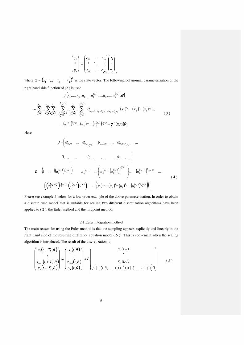
2.1 Euler integration method

The main reason for using the Euler method is that the sampling appears explicitly and linearly in the

right hand side of the resulting difference equation model ( 5 ) . This is convenient when the scaling

algorithm is introduced. The result of the discretization is

( 5 )

7

.

( 6 )

It can be remarked that the Euler method may require fast sampling in order not to introduce

significant discretization errors. This is fortunately a less important effect in system identification

applications. The reason is that the minimization algorithm uses the parameters as instruments to fit

the model output to the measured data, as expressed by the criterion function. Even if an additional

bias would be introduced in the estimated parameters, the input-output properties of the identified

model can be expected to describe the data well.

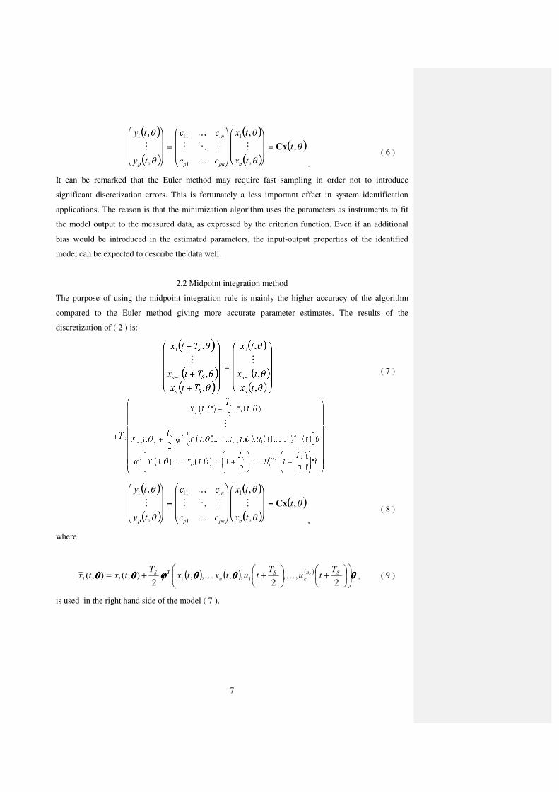
2.2 Midpoint integration method

The purpose of using the midpoint integration rule is mainly the higher accuracy of the algorithm

compared to the Euler method giving more accurate parameter estimates. The results of the

discretization of ( 2 ) is:

( 7 )

,

( 8 )

where

( ) ( ) ( ) θθθθθθθθθθθθϕϕϕϕθθθθθθθθ

+

++=

2,,

2,,,,

2),(),( 11

Sn

k

S

n

TS

ii

Ttu

Ttutxtx

Ttxtx kKK ,

( 9 )

is used in the right hand side of the model ( 7 ).

8

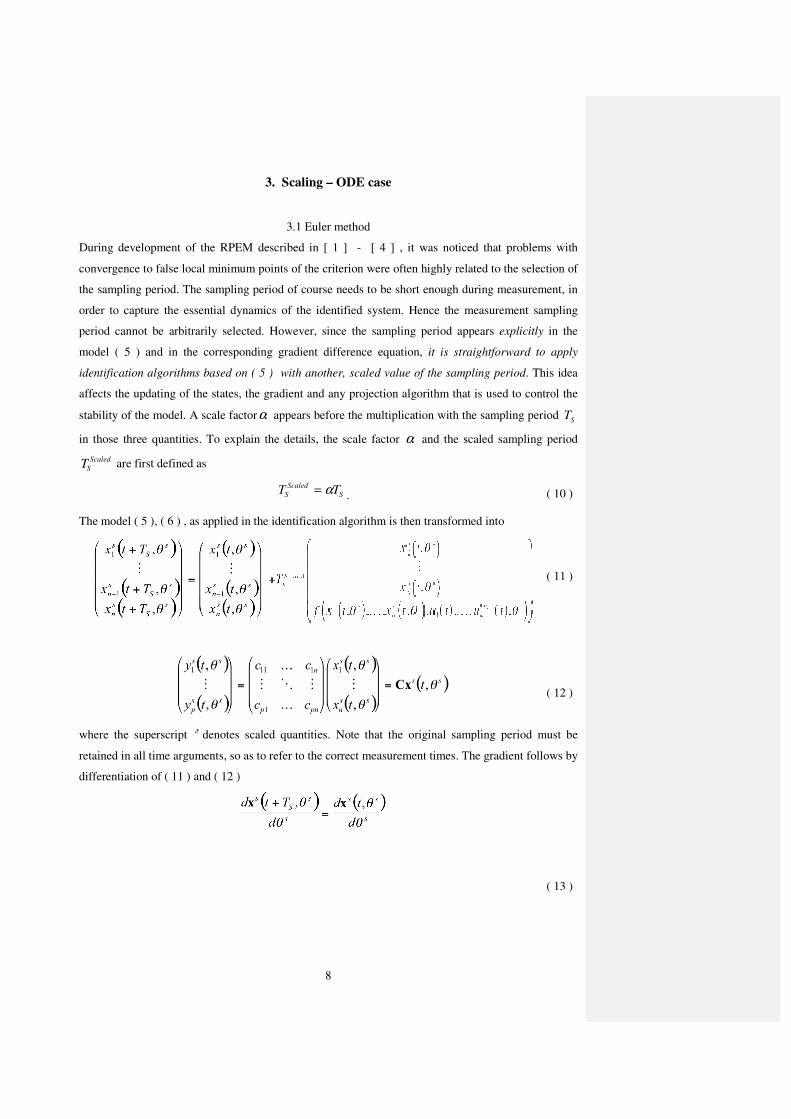
3. Scaling – ODE case

3.1 Euler method

During development of the RPEM described in [ 1 ] - [ 4 ] , it was noticed that problems with

convergence to false local minimum points of the criterion were often highly related to the selection of

the sampling period. The sampling period of course needs to be short enough during measurement, in

order to capture the essential dynamics of the identified system. Hence the measurement sampling

period cannot be arbitrarily selected. However, since the sampling period appears explicitly in the

model ( 5 ) and in the corresponding gradient difference equation, it is straightforward to apply

identification algorithms based on ( 5 ) with another, scaled value of the sampling period. This idea

affects the updating of the states, the gradient and any projection algorithm that is used to control the

stability of the model. A scale factorα appears before the multiplication with the sampling period TS

in those three quantities. To explain the details, the scale factor α and the scaled sampling period

TS

Scaled are first defined as

T TS

Scaled

S= α . ( 10 )

The model ( 5 ), ( 6 ) , as applied in the identification algorithm is then transformed into

( 11 )

( 12 )

where the superscript denotes scaled quantities. Note that the original sampling period must be

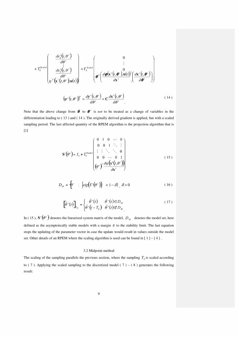
retained in all time arguments, so as to refer to the correct measurement times. The gradient follows by

differentiation of ( 11 ) and ( 12 )

( 13 )

9

( ) ( )( ) ( )

+

s

ss

s

ssT

Scaled

S

d

td

d

ttd

T

θθθθ

θθθθθθθθϕϕϕϕθθθθ

,,,

0

0

x

x

ux

M

( )( ) ( ) ( )s

ss

s

ssTss

d

td

d

tdt

θ

θ

θ

θθψ

,,,

xC

y==

. ( 14 )

Note that the above change from θθθθ to sθθθθ is not to be treated as a change of variables in the

differentiation leading to ( 13 ) and ( 14 ). The originally derived gradient is applied, but with a scaled

sampling period. The last affected quantity of the RPEM algorithm is the projection algorithm that is

[1]

( 15 )

}1 − δ , δ > 0 ( 16 )

.

( 17 )

In ( 15 ), denotes the linearized system matrix of the model, denotes the model set, here

defined as the asymptotically stable models with a margin to the stability limit. The last equation

stops the updating of the parameter vector in case the update would result in values outside the model

set. Other details of an RPEM where the scaling algorithm is used can be found in [ 1 ] – [ 4 ] .

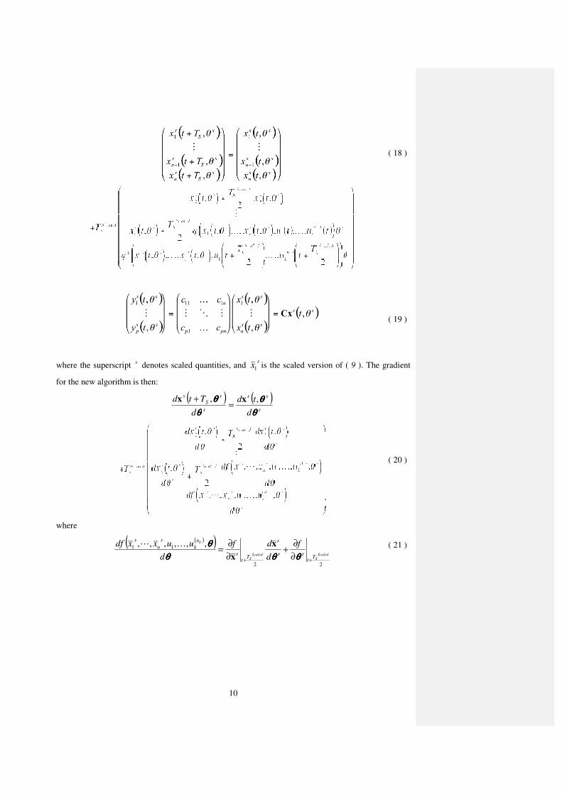
3.2 Midpoint method

The scaling of the sampling parallels the previous section, where the sampling ST is scaled according

to ( 7 ). Applying the scaled sampling to the discretized model ( 7 ) – ( 8 ) generates the following

result:

10

( 18 )

( 19 )

where the superscript s denotes scaled quantities, and

sx1 is the scaled version of ( 9 ). The gradient

for the new algorithm is then:

( ) ( )s

ss

s

s

S

s

d

td

d

Ttd

θθθθ

θθθθ

θθθθ

θθθθ ,, xx=

+

( 20 )

where

( )( )22

11 ,,,,,,Scaled

SScaled

S

k

Tt

ss

s

Tt

s

n

k

s

n

sf

d

df

d

uuxxdf

++ ∂

∂+

∂

∂=

θθθθθθθθθθθθ

θθθθ x

x

KL ( 21 )

11

( ) ( )( )

( )

∂

∂

+

+=

ss

Scaled

S

ss

s

ss

s

s

t

f

T

tutd

td

d

d

θθθθ

θθθθϕϕϕϕθθθθ

θθθθ

θθθθ

,

1000

0

100

0010

2

)(,,,

x

xxx

L

OOMM

MO

L

( )( )

( ) ( )( )( )

( )s

ss

ss

ssTs

s

ss

s

d

td

td

tdf

ttf

θθθθ

θθθθ

θθθθ



,

,

,

)(,,

x

x

x

x

ux

=∂

∂

=∂

∂

( 22 )

( 23 )

( 24 )

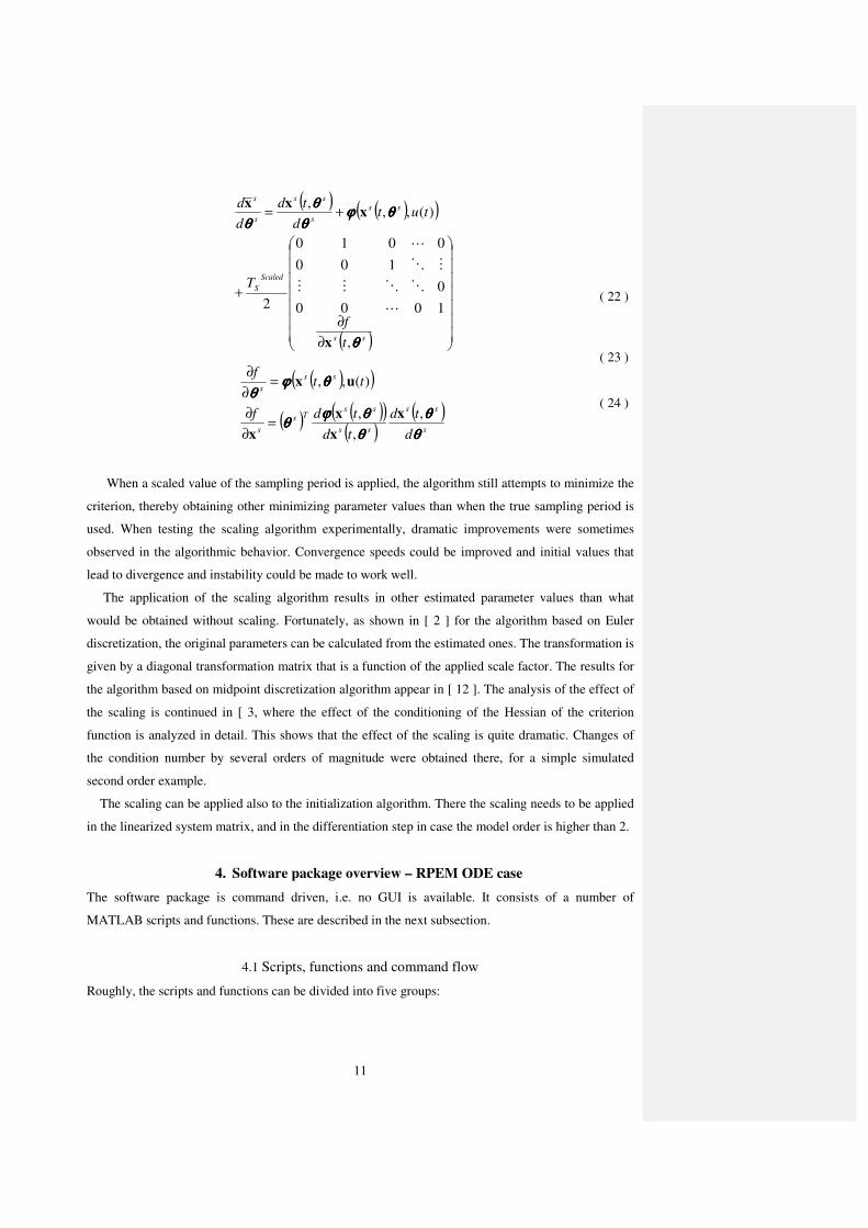
When a scaled value of the sampling period is applied, the algorithm still attempts to minimize the

criterion, thereby obtaining other minimizing parameter values than when the true sampling period is

used. When testing the scaling algorithm experimentally, dramatic improvements were sometimes

observed in the algorithmic behavior. Convergence speeds could be improved and initial values that

lead to divergence and instability could be made to work well.

The application of the scaling algorithm results in other estimated parameter values than what

would be obtained without scaling. Fortunately, as shown in [ 2 ] for the algorithm based on Euler

discretization, the original parameters can be calculated from the estimated ones. The transformation is

given by a diagonal transformation matrix that is a function of the applied scale factor. The results for

the algorithm based on midpoint discretization algorithm appear in [ 12 ]. The analysis of the effect of

the scaling is continued in [ 3, where the effect of the conditioning of the Hessian of the criterion

function is analyzed in detail. This shows that the effect of the scaling is quite dramatic. Changes of

the condition number by several orders of magnitude were obtained there, for a simple simulated

second order example.

The scaling can be applied also to the initialization algorithm. There the scaling needs to be applied

in the linearized system matrix, and in the differentiation step in case the model order is higher than 2.

4. Software package overview – RPEM ODE case

The software package is command driven, i.e. no GUI is available. It consists of a number of

MATLAB scripts and functions. These are described in the next subsection.

4.1 Scripts, functions and command flow

Roughly, the scripts and functions can be divided into five groups:

12

• Live data measurements. The two scripts of this group set up and perform clocked live data

measurements. The scripts are SetupLive.m and MeasurementMain.m.

• Simulated data generation. The four scripts of this group define a dynamic system, that is then

used for generation of simulated data. The scripts and functions are SetupData.m, f.m, h.m and

GenerateData.m.

• Recursive identification. The five scripts of this group perform the actual identification tasks,

supporting user interaction. The scripts and functions are SetupRPEM.m, RPEM.m, h_m.m,

dhdx_m.m and ReInitiate.m.

• Supporting functions - not called by the user. The four functions of this group are called by scripts

of the previous group. They are all related to the implementation of the RHS model of the

identified ODE. The scripts are GenerateIndices.m, f_m.m, dfdx_m.m and dfdtheta_m.m.

• Preparation and display of results. There are eleven scripts in this group. They all prepare,

compute and display results of the identification process. The scripts are PlotData.m,

SimulateModelOutput.m, PlotParameters.m, PlotPredictionErrors.m, PlotEigenvalues.m,

PlotCondition.m, ComputeRPEMLossFunction.m, PlotModelOutput.m,

PlotSystemAndModelOutput.m, PlotResidualErrors.m and MeanResidualAnalysis.m.

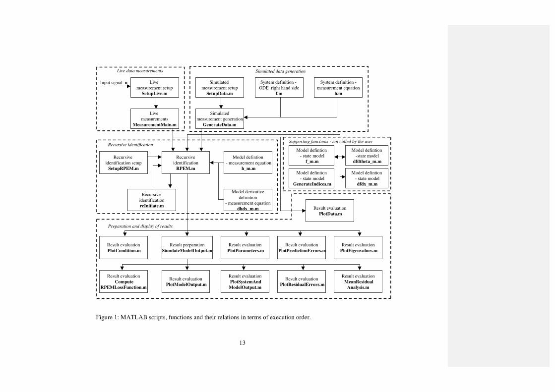
These groups of scripts and functions need to be operated in a particular order to make sense. This

order of execution between scripts and functions is displayed with arrows in Figure 1. A single

directional arrow indicates that the script/function pointed at may be executed only after the execution

of the pointing script/function. See Figure 1 for details.

There are three major ways to exploit the five groups of scripts and functions.

1. In case the user has input and output signals available, the first step is to define and run the script

SetupLive.m. This sets basic parameters like the sampling period. The user can then proceed

directly to use the groups Recursive Identification and Preparation and display of results. The

data, which can be simulated or live, should be stored in the (row) matrices u and y .

2. In case the user is to perform live measurements, all the steps of the Live data measurement group

should be executed first. The user can then proceed directly to use the groups Recursive

Identification and Preparation and display of results.

3. In case the user intends to use simulated data, this data can be generated by execution of the

scripts and functions of the group Simulated data generation. The user can then proceed directly

to use the groups Recursive Identification and Preparation and display of results.

13

Figure 1: MATLAB scripts, functions and their relations in terms of execution order.

Live

measurement setup

SetupLive.m

Live

measurements

MeasurementMain.m

Input signal u

Live data measurements

Simulated

measurement setup

SetupData.m

Simulated

measurement generation

GenerateData.m

System definition -

measurement equation

h.m

System definition -

ODE right hand side

f.m

Simulated data generation

Recursive

identification

RPEM.m

Recursive

identification setup

SetupRPEM.m

Model defintion

- measurement equation

h_m.m

Model derivative

definition

- measurement equation

dhdx_m.m

Recursive

identification

reInitiate.m

Recursive identification

Result evaluation

PlotModelOutput.m

Result evaluation

PlotSystemAnd

ModelOutput.m

Result evaluation

PlotResidualErrors.m

Result evaluation

PlotCondition.m

Result evaluation

PlotEigenvalues.m

Result evaluation

PlotPredictionErrors.m

Result evaluation

PlotParameters.m

Result preparation

SimulateModelOutput.m

Result evaluation

Compute

RPEMLossFunction.m

Result evaluation

MeanResidual

Analysis.m

Result evaluation

PlotData.m

Preparation and display of results

Model defintion

-state model

dfdtheta_m.m

Model defintion

- state model

f_m.m

Model defintion

- state model

dfdx_m.m

Model defintion

- state model

GenerateIndices.m

Supporting functions - not called by the user

14

4.2 Restrictions

The main restrictions of the software are

• The software is command line driven - no GUI support is implemented.

• The software does not support true real time operation - there is no real time OS support

implemented.

• The software has been tested and run using MATLAB 5.3, MATLAB 6.5, MATLAB 7.0 and

MATLAB 7.9..

5. Data input – RPEM ODE case

The generation of data begins the section where the actual software is described. Since the user has

access to all source files, the descriptions below do not describe code related issues and internal

variables. Only the parts that are required for the use of the software package are covered. When m-

files are reproduced, only the relevant parts are included, the reader should be aware that more

information can be found in the source code. Note that the setup files are to be treated as templates, the

user is hence required to modify right hand sides only - no addition or deletion of code should be used

in the normal use of the package.

5.1 Simulated data

The generation of simulated data requires that the user

1. Modifies the underlying ODE model, as given by f.m and h.m. The function f.m implements the

RHS of the ODE, using a conventional MATLAB function call. Note that the built in ODE solvers

of MATLAB are not used. Instead an Euler algorithm is implemented. The reason is that this

allows the generation of simulated data that can be exactly described by the applied model, should

this be desired. The function h.m implements the (possibly nonlinear) measurement equation. The

functions allow for addition of systems noise and measurement noise.

2. Provides further input data in the script SetupData.m. The parameters that define the data

generation are directly written into this script. These parameters define the sampling period, the

data length, the dimensions of the system, the type and parameters of the input signal, the type and

parameters of the disturbances, as well as the initial value of the ODE.

3. Executes SetupData.m. This loads the necessary parameters into the MATLAB workspace.

4. Generates data by execution of GenerateData.m. After the execution of this script, variables with

sampling instances, input signals and output signals are available in the MATLAB workspace.

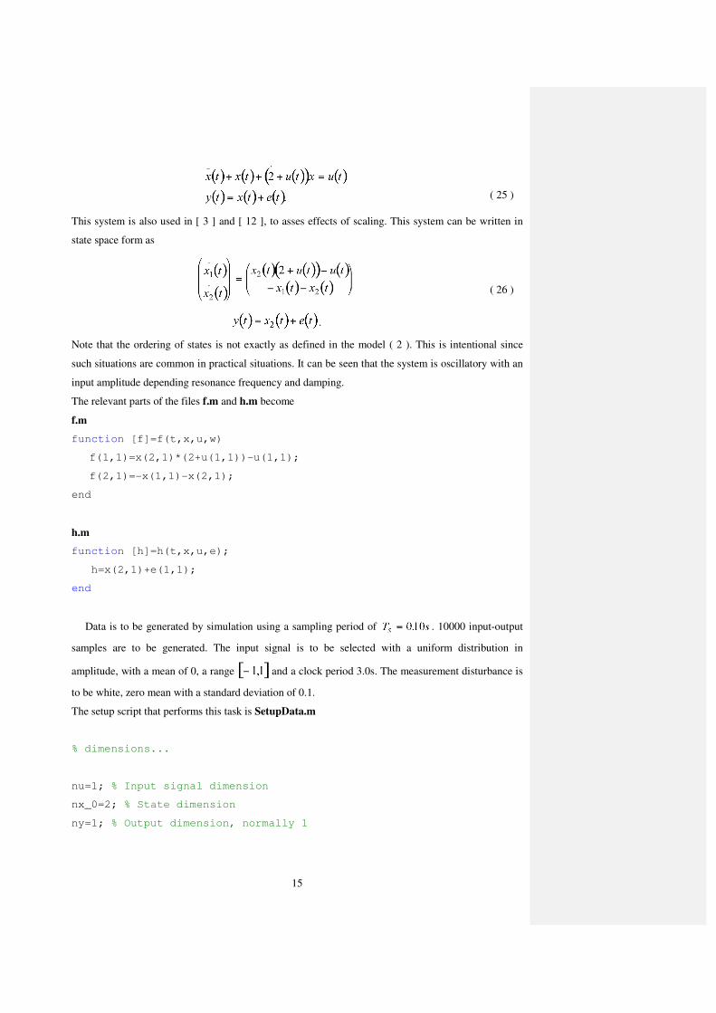
Example 1: This and the following examples illustrates the use of the software package for

identification of the system

15

( 25 )

This system is also used in [ 3 ] and [ 12 ], to asses effects of scaling. This system can be written in

state space form as

.

( 26 )

Note that the ordering of states is not exactly as defined in the model ( 2 ). This is intentional since

such situations are common in practical situations. It can be seen that the system is oscillatory with an

input amplitude depending resonance frequency and damping.

The relevant parts of the files f.m and h.m become

f.m

function [f]=f(t,x,u,w)

f(1,1)=x(2,1)*(2+u(1,1))-u(1,1);

f(2,1)=-x(1,1)-x(2,1);

end

h.m

function [h]=h(t,x,u,e);

h=x(2,1)+e(1,1);

end

Data is to be generated by simulation using a sampling period of . 10000 input-output

samples are to be generated. The input signal is to be selected with a uniform distribution in

amplitude, with a mean of 0, a range and a clock period 3.0s. The measurement disturbance is

to be white, zero mean with a standard deviation of 0.1.

The setup script that performs this task is SetupData.m

% dimensions...

nu=1; % Input signal dimension

nx_0=2; % State dimension

ny=1; % Output dimension, normally 1

16

% Input signal related...Type may be selected among:

%

% InputType=[

% 'PRBS ';

% 'Gaussian ';

% 'UniformPRBS';

% 'SineWave ';

% 'Custom '];

InputType=[

'UniformPRBS'];

uAmplitude=[

1.0];

uMean=[

0];

uFrequency=[

0.1];

ClockPeriod=[

30];% Clock period vector in terms of sampling time

% System disturbance related...Type may be selected among:

%

% DisturbanceTypeSystem=[

% 'WGN ';

% 'SineWave';

% 'Custom '];

DisturbanceTypeSystem=[

'WGN ';

'WGN '];

wSigma=[

0.0;

0.0]; % Gaussian system noise standard deviation (discrete time)

wMean=[

0;

0];

wSineAmplitude=[

17

0;

0];

wSineFrequency=[

0;

0];

% Measurement disturbance related... Type may be selected among:

%

% DisturbanceTypeMeasuremet=[

% 'WGN ';

% 'SineWave';

% 'Custom '];

DisturbanceTypeMeasurement=[

'WGN '];

eSigma=0.1; % Gaussian measurement noise standard deviation

eMean=[

0;

0];

eSineAmplitude=[

0];

eSineFrequency=[

0];

% sampling time and data length

Ts=0.1; % Sampling time in seconds

N=10000; % Number of data points

SamplingInstances=(Ts:Ts:N*Ts);

% ODE related...

x0=[0.5 -1.0]'; % Initial values

The final step of the data generation is to execute the files SetupData.m and GenerateData.m.

This is done in the MATLAB command window as follows

18

» SetupData

» GenerateData

…

percentReady =

100

»

5.2 Live data

The generation of simulated data requires that the user

1. Is connected to the system via MATLAB. The connection must be such that commands to control

DA-converters that generate input signals can be issued from within MATLAB. Similarly,

commands that read AD-converters that sample output signals must be available from within

MATLAB. The script MeasurementMain.m probably needs modification in a few parts in order

to interface correctly to the AD- and DA-converters of the system of the user.

2. Generates an input signal, that is stored in the matrix (row vector in the one-dimensional input

signal case) .

3. Provides further data in the script SetupLive.m. The parameters that define the data generation are

directly written into this script. These parameters defines the sampling period, the data length and

the dimensions of the system.

4. Executes SetupLive.m. This loads the necessary parameters into the MATLAB workspace.

5. Generates data by execution of MeasurementMain.m. After the execution of this file, variables

with input signals and output signals are available in the MATLAB workspace. This script operates

as a loop that continuously polls the MATLAB real time clock, waiting for the next sampling

instance. This means that it may not be possible to use the computer for other tasks during the data

collection session. The reason for this solution is that it avoids the need for a real time OS

connection. Note also that the calls to AD- and DA-converters may be different on other systems.

This script is hence likely to require some modification.

Example 2: The setup script file SetupLive.m becomes (empty since simulated data is used here)

% dimensions...Note that nx is not really relevant,

% it is however required in the RPEM setup so it is set in this file

nu=[]; % Input signal dimension

nx=[]; % State dimension

ny=[]; % Output dimension, normally 1

% sampling time and data length

19

Ts=[]; % Sampling time in seconds

N=[]; % Number of data points

SamplingInstances=(Ts:Ts:N*Ts);

The measurement process is started by typing

» SetupData

» GenerateData

…

in the MATLAB command window. During the measurement session, the script continuously displays

the time, the inputs as well as the measured outputs, as commanded to DA-converters and read by AD-

converters. After termination all data that is needed for identification is available in the MATLAB

workspace.

5.3 Display of data

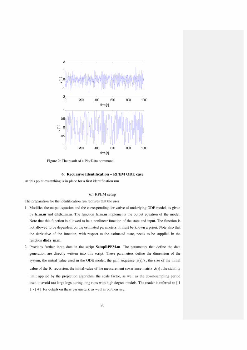
After execution of either one of the chain of actions of section 5.1 or section 5.2, data can be plotted.

1. The PlotData.m script that is executed in the MATLAB command window. This script makes use

of the dimensions of the system in order to divide the plot into several sub-windows, and in order

to provide the axis text.

Example 3: The MATLAB command window command is

» PlotData

»

The following plot is generated

20

Figure 2: The result of a PlotData command.

6. Recursive Identification – RPEM ODE case

At this point everything is in place for a first identification run.

6.1 RPEM setup

The preparation for the identification run requires that the user

1. Modifies the output equation and the corresponding derivative of underlying ODE model, as given

by h_m.m and dhdx_m.m. The function h_m.m implements the output equation of the model.

Note that this function is allowed to be a nonlinear function of the state and input. The function is

not allowed to be dependent on the estimated parameters, it must be known a priori. Note also that

the derivative of the function, with respect to the estimated state, needs to be supplied in the

function dhdx_m.m.

2. Provides further input data in the script SetupRPEM.m. The parameters that define the data

generation are directly written into this script. These parameters define the dimension of the

system, the initial value used in the ODE model, the gain sequence ( )µ t t , the size of the initial

value of the R -recursion, the initial value of the measurement covariance matrix ( )ΛΛΛΛ t , the stability

limit applied by the projection algorithm, the scale factor, as well as the down-sampling period

used to avoid too large logs during long runs with high degree models. The reader is referred to [ 1

] - [ 4 ] for details on these parameters, as well as on their use.

0 200 400 600 800 1000-2

-1

0

1

2

time [s]

y(1

)

0 200 400 600 800 1000-1

-0.5

0

0.5

1

time [s]

u(1

)

21

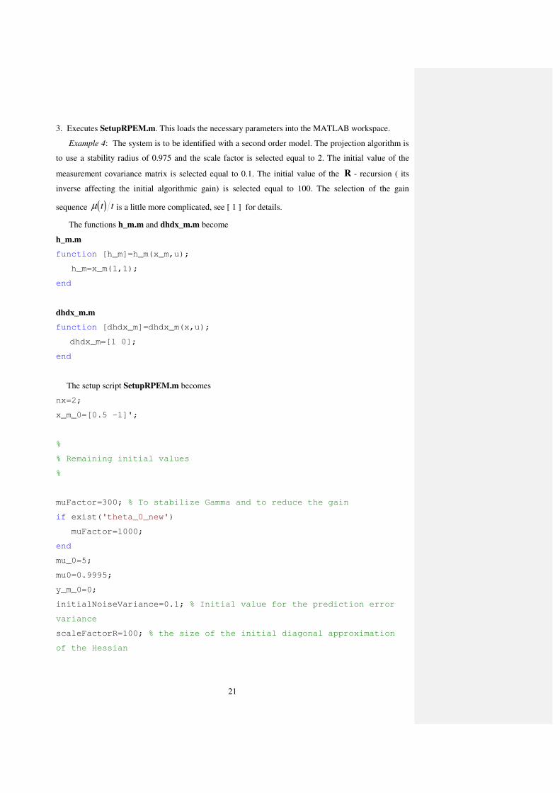
3. Executes SetupRPEM.m. This loads the necessary parameters into the MATLAB workspace.

Example 4: The system is to be identified with a second order model. The projection algorithm is

to use a stability radius of 0.975 and the scale factor is selected equal to 2. The initial value of the

measurement covariance matrix is selected equal to 0.1. The initial value of the R - recursion ( its

inverse affecting the initial algorithmic gain) is selected equal to 100. The selection of the gain

sequence ( )µ t t is a little more complicated, see [ 1 ] for details.

The functions h_m.m and dhdx_m.m become

h_m.m

function [h_m]=h_m(x_m,u);

h_m=x_m(1,1);

end

dhdx_m.m

function [dhdx_m]=dhdx_m(x,u);

dhdx_m=[1 0];

end

The setup script SetupRPEM.m becomes

nx=2;

x_m_0=[0.5 -1]';

%

% Remaining initial values

%

muFactor=300; % To stabilize Gamma and to reduce the gain

if exist('theta_0_new')

muFactor=1000;

end

mu_0=5;

mu0=0.9995;

y_m_0=0;

initialNoiseVariance=0.1; % Initial value for the prediction error

variance

scaleFactorR=100; % the size of the initial diagonal approximation

of the Hessian

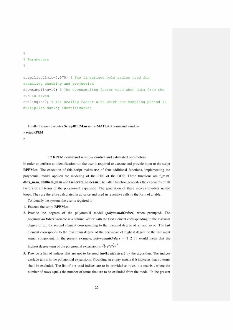
22

%

% Parameters

%

stabilityLimit=0.975; % The linearized pole radius used for

stability checking and projection

downSampling=10; % The downsampling factor used when data from the

run is saved

scalingTs=2; % The scaling factor with which the sampling period is

multiplied during identification

Finally the user executes SetupRPEM.m in the MATLAB command window

» setupRPEM

»

6.2 RPEM command window control and estimated parameters

In order to perform an identification run the user is required to execute and provide input to the script

RPEM.m. The execution of this script makes use of four additional functions, implementing the

polynomial model applied for modeling of the RHS of the ODE. These functions are f_m.m,

dfdx_m.m, dfdtheta_m.m and GenerateIndices.m. The latter function generates the exponents of all

factors of all terms of the polynomial expansion. The generation of these indices involves nested

loops. They are therefore calculated in advance and used in repetitive calls in the form of a table.

To identify the system, the user is required to

1. Execute the script RPEM.m

2. Provide the degrees of the polynomial model (polynomialOrders) when prompted. The

polynomialOrders variable is a column vector with the first element corresponding to the maximal

degree of x1 , the second element corresponding to the maximal degree of x2 and so on. The last

element corresponds to the maximum degree of the derivative of highest degree of the last input

signal component. In the present example, polynomialOrders = [1 2 3]' would mean that the

highest degree term of the polynomial expansion is θ123 1 22 3

x x u .

3. Provide a list of indices that are not to be used (notUsedIndices) by the algorithm. The indices

exclude terms in the polynomial expansions. Providing an empty matrix ([]) indicates that no terms

shall be excluded. The list of not used indices are to be provided as rows in a matrix , where the

number of rows equals the number of terms that are to be excluded from the model. In the present

23

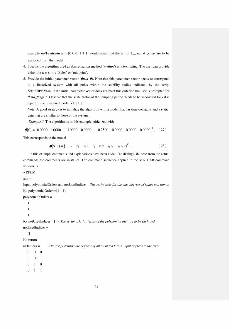
example notUsedIndices = [0 0 0; 1 1 1] would mean that the terms θ000 and θ111 1 2x x u are to be

excluded from the model.

4. Specify the algorithm used as discretization method (method) as a text string. The user can provide

either the text string ‘Euler’ or ‘midpoint’.

5. Provide the initial parameter vector (theta_0). Note that this parameter vector needs to correspond

to a linearized system with all poles within the stability radius indicated by the script

SetupRPEM.m. If the initial parameter vector does not meet this criterion the user is prompted for

theta_0 again. Observe that the scale factor of the sampling period needs to be accounted for - it is

a part of the linearized model, cf. [ 1 ].

Note: A good strategy is to initialize the algorithm with a model that has time constants and a static

gain that are similar to those of the system.

Example 5: The algorithm is in this example initialized with

( ) ( )$ . . . . . . . .θθθθ 0 0 0000 10000 10000 0 0000 0 2500 0 0000 0 0000 0 0000= − −T

. ( 27 )

This corresponds to the model

( ) ( )ϕϕϕϕ x,u u x x u x x u x x x x uT

= 1 2 2 1 1 1 2 1 2 . ( 28 )

In this example comments and explanations have been added. To distinguish these from the actual

commands the comments are in italics. The command sequence applied in the MATLAB command

window is

» RPEM

ans =

Input polynomialOrders and notUsedIndices - The script asks for the max degrees of states and inputs

K» polynomialOrders=[1 1 1]'

polynomialOrders =

1

1

1

K» notUsedIndices=[] - The script asks for terms of the polynomial that are to be excluded

notUsedIndices =

[]

K» return

allIndices = - The script returns the degrees of all included terms, input degrees to the right

0 0 0

0 0 1

0 1 0

0 1 1

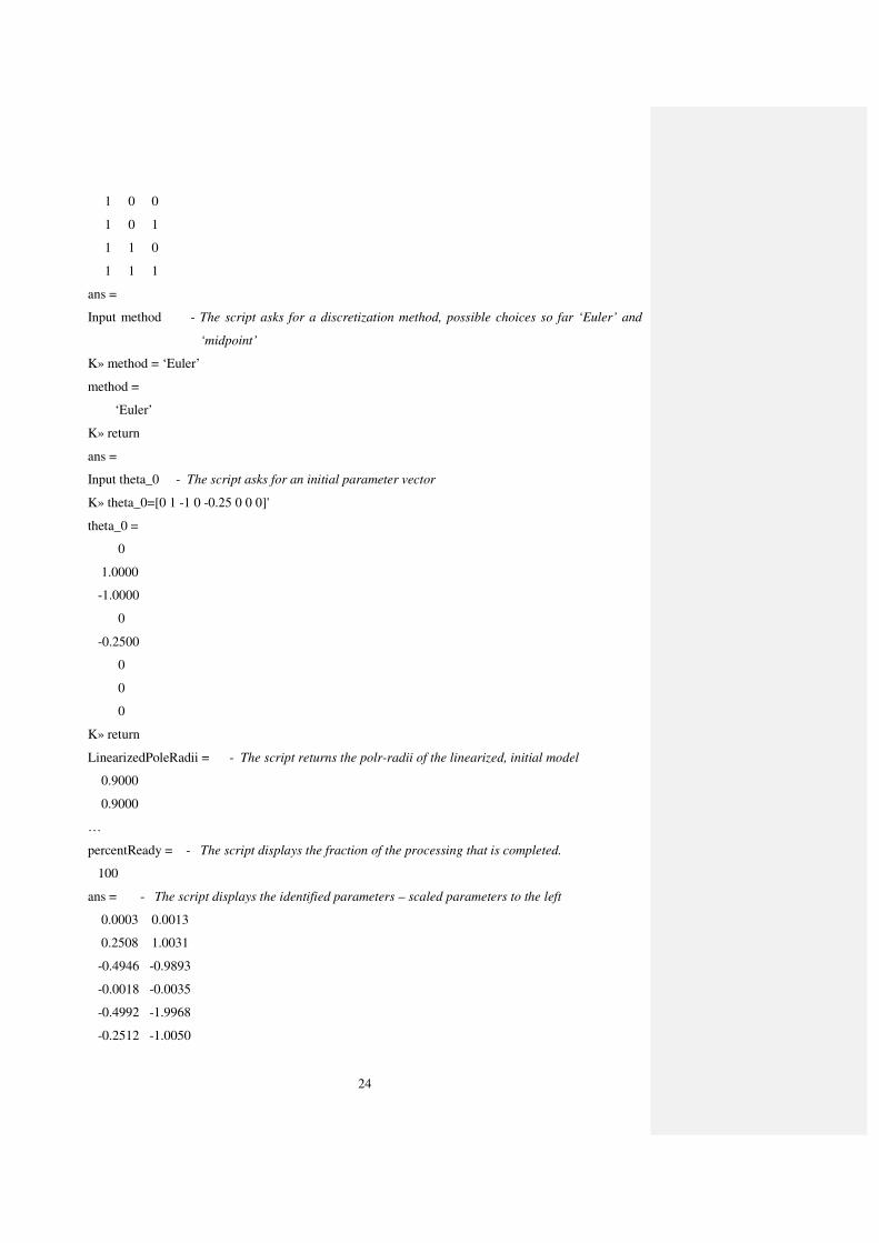
24

1 0 0

1 0 1

1 1 0

1 1 1

ans =

Input method - The script asks for a discretization method, possible choices so far ‘Euler’ and

‘midpoint’

K» method = ‘Euler’

method =

‘Euler’

K» return

ans =

Input theta_0 - The script asks for an initial parameter vector

K» theta_0=[0 1 -1 0 -0.25 0 0 0]'

theta_0 =

0

1.0000

-1.0000

0

-0.2500

0

0

0

K» return

LinearizedPoleRadii = - The script returns the polr-radii of the linearized, initial model

0.9000

0.9000

…

percentReady = - The script displays the fraction of the processing that is completed.

100

ans = - The script displays the identified parameters – scaled parameters to the left

0.0003 0.0013

0.2508 1.0031

-0.4946 -0.9893

-0.0018 -0.0035

-0.4992 -1.9968

-0.2512 -1.0050

25

0.0163 0.0326

-0.0174 -0.0347

»

The estimated parameters of the left column correspond to the ones obtained directly from the RPEM,

i.e. these are scaled parameters. The right column contain parameters that are recomputed to

correspond to the original sampling period. Note that the exact result depends on the generated input

signal. This may differ between systems and execution occasions since the seed for the random

number generator may differ. Hence, slight variations of the estimated parameters are normal.

6.3 Re-initiation, multiple runs and iterative refinement

The script RPEM.m produces a result for a certain choice of degrees of the right hand polynomial of

the ODE (if the stability check is not triggered so that the algorithm gets stuck close to the stability

limit). In case the result is not deemed sufficient, then a higher degree right hand side may be needed.

The opposite may also be true, i.e. the result is sufficient but the number of parameters used may be

unnecessarily high. So there is a need to

• Modify the degrees of the polynomial model of the ODE.

• Remove specific terms of the polynomial model of the ODE.

• Rerun the RPEM from the previous end results, with a redefined right hand side polynomial.

Exactly this is supported by the script reInitiate.m.

Note: Support for stepping also of the model order would be preferred. Such stepping does however

have complicated (nonlinear) stability impacts. For this reason the development of such functionality

is postponed to later versions of the software package.

In order to perform a new RPEM run with modified degrees, then user is required to

1. Run the script reInitiate.m. That script prompts the user for polynomialOrders and

notUsedIndices. The parameter vector at the end of the run, together with the previous and new

degrees, are then used to re-initiate all relevant quantities of the RPEM.

2. Rerun RPEM.m. Note that the RPEM does not need to prompt the user for any further information

this time.

Example 6: In this example the degree of the input signal is increased to 2.

The MATLAB command window commands become

» reInitiate

ans =

Input polynomialOrders and notUsedIndices

K» polynomialOrders=[1 1 2]'

polynomialOrders =

1

1

26

2

K» return

» RPEM

…

The identification is now finalized and everything is set for display of the results.

7. Display of results – RPEM ODE case

The display of results is straightforward. By a study of the source code, users should be able to tailor

available scripts and also write own ones when needed.

7.1 Parameters

In order to plot the parameters the user is required to

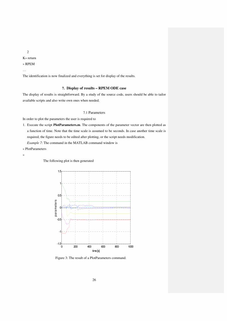
1. Execute the script PlotParameters.m. The components of the parameter vector are then plotted as

a function of time. Note that the time scale is assumed to be seconds. In case another time scale is

required, the figure needs to be edited after plotting, or the script needs modification.

Example 7: The command in the MATLAB command window is

» PlotParameters

»

The following plot is then generated

Figure 3: The result of a PlotParameters command.

0 200 400 600 800 1000-1.5

-1

-0.5

0

0.5

1

1.5

time [s]

pa

ram

ete

rs

27

7.2 Prediction errors

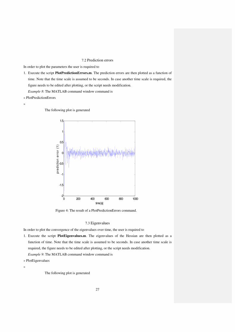
In order to plot the parameters the user is required to

1. Execute the script PlotPredictionErrors.m. The prediction errors are then plotted as a function of

time. Note that the time scale is assumed to be seconds. In case another time scale is required, the

figure needs to be edited after plotting, or the script needs modification.


» PlotPredictionErrors

»


Figure 4: The result of a PlotPredictionErrors command.

7.3 Eigenvalues

In order to plot the convergence of the eigenvalues over time, the user is required to

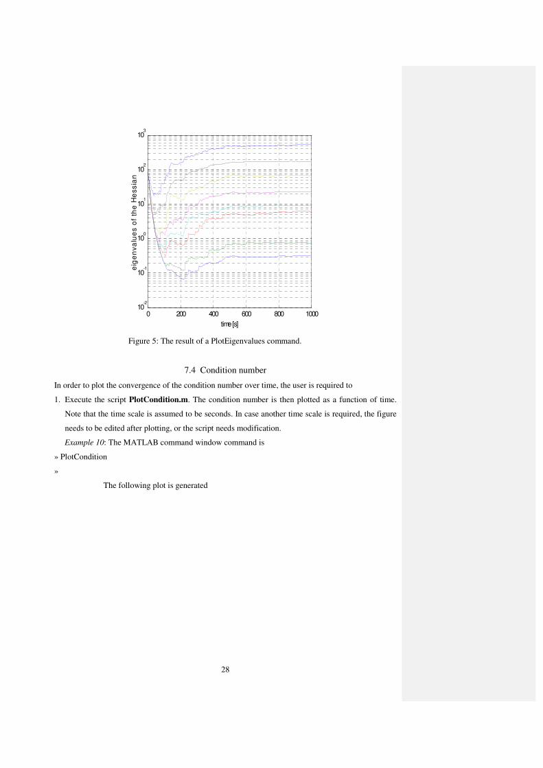
1. Execute the script PlotEigenvalues.m. The eigenvalues of the Hessian are then plotted as a

function of time. Note that the time scale is assumed to be seconds. In case another time scale is



» PlotEigenvalues

»


0 200 400 600 800 1000-2

-1.5

-1

-0.5

0

0.5

1

1.5

time [s]

pre

dic

tio

n e

rro

r (1

)

28

Figure 5: The result of a PlotEigenvalues command.

7.4 Condition number

In order to plot the convergence of the condition number over time, the user is required to

1. Execute the script PlotCondition.m. The condition number is then plotted as a function of time.

Note that the time scale is assumed to be seconds. In case another time scale is required, the figure

needs to be edited after plotting, or the script needs modification.


» PlotCondition

»


0 200 400 600 800 100010

-2

10-1

100

101

102

103

time [s]

eig

en

va

lue

s o

f th

e H

es

sia

n

29

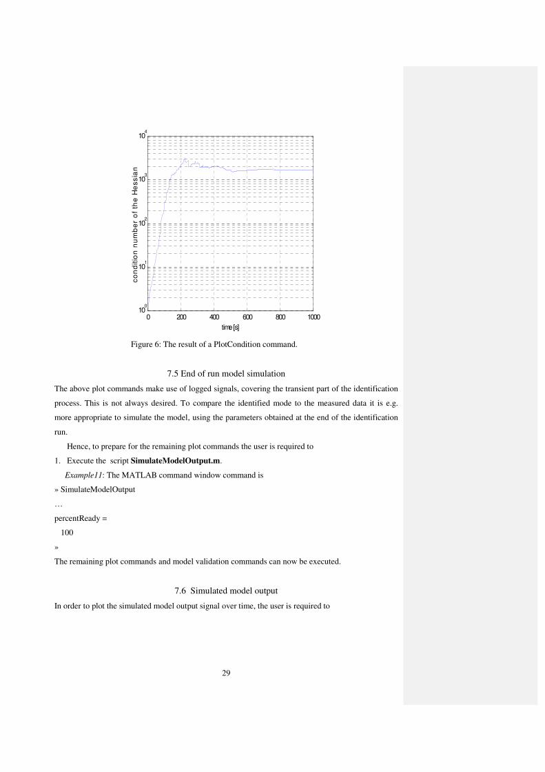
Figure 6: The result of a PlotCondition command.

7.5 End of run model simulation

The above plot commands make use of logged signals, covering the transient part of the identification

process. This is not always desired. To compare the identified mode to the measured data it is e.g.

more appropriate to simulate the model, using the parameters obtained at the end of the identification

run.

Hence, to prepare for the remaining plot commands the user is required to

1. Execute the script SimulateModelOutput.m.

Example11: The MATLAB command window command is

» SimulateModelOutput

…

percentReady =

100

»

The remaining plot commands and model validation commands can now be executed.

7.6 Simulated model output

In order to plot the simulated model output signal over time, the user is required to

0 200 400 600 800 100010

0

101

102

103

104

time [s]

co

nd

itio

n n

um

be

r o

f th

e H

ess

ian

30

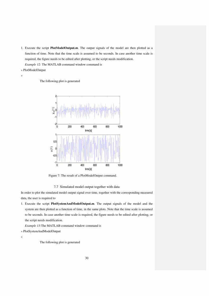
1. Execute the script PlotModelOutput.m. The output signals of the model are then plotted as a

function of time. Note that the time scale is assumed to be seconds. In case another time scale is



» PlotModelOutput

»


Figure 7: The result of a PlotModelOutput command.

7.7 Simulated model output together with data

In order to plot the simulated model output signal over time, together with the corresponding measured

data, the user is required to

1. Execute the script PlotSystemAndModelOutput.m. The output signals of the model and the

system are then plotted as a function of time, in the same plots. Note that the time scale is assumed

to be seconds. In case another time scale is required, the figure needs to be edited after plotting, or

the script needs modification.

Example 13:The MATLAB command window command is

» PlotSystemAndModelOutput

»


0 200 400 600 800 1000-2

-1

0

1

2

time [s]

ym

(1)

0 200 400 600 800 1000-1

-0.5

0

0.5

1

time [s]

u(1

)

31

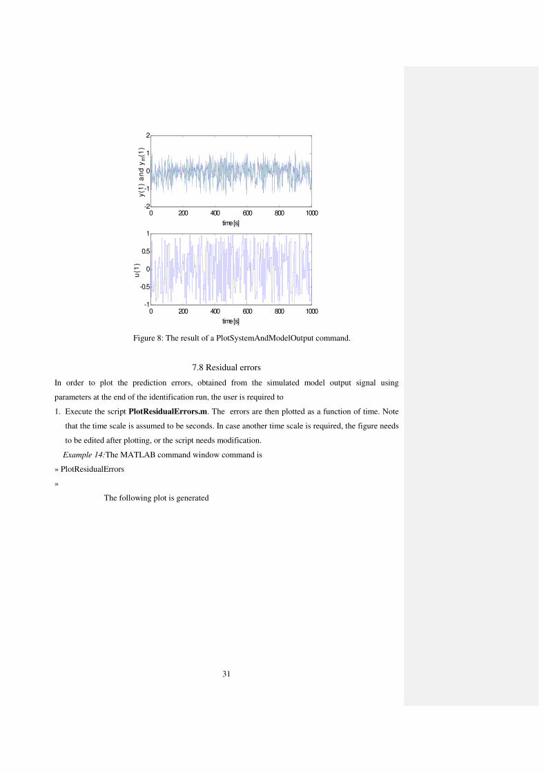
Figure 8: The result of a PlotSystemAndModelOutput command.

7.8 Residual errors

In order to plot the prediction errors, obtained from the simulated model output signal using

parameters at the end of the identification run, the user is required to

1. Execute the script PlotResidualErrors.m. The errors are then plotted as a function of time. Note

that the time scale is assumed to be seconds. In case another time scale is required, the figure needs

to be edited after plotting, or the script needs modification.

Example 14:The MATLAB command window command is

» PlotResidualErrors

»


0 200 400 600 800 1000-2

-1

0

1

2

time [s]

y(1

) a

nd

ym

(1)

0 200 400 600 800 1000-1

-0.5

0

0.5

1

time [s]

u(1

)

32

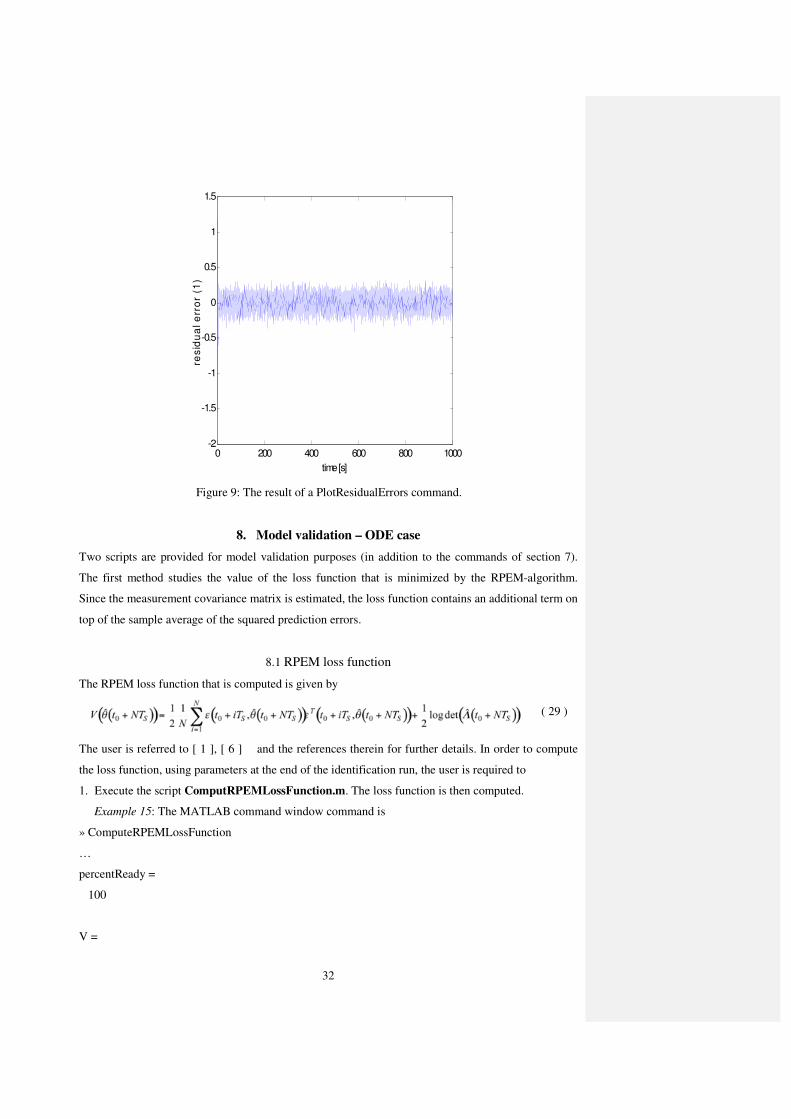
Figure 9: The result of a PlotResidualErrors command.

8. Model validation – ODE case

Two scripts are provided for model validation purposes (in addition to the commands of section 7).

The first method studies the value of the loss function that is minimized by the RPEM-algorithm.

Since the measurement covariance matrix is estimated, the loss function contains an additional term on

top of the sample average of the squared prediction errors.

8.1 RPEM loss function

The RPEM loss function that is computed is given by

( 29 )

The user is referred to [ 1 ], [ 6 ] and the references therein for further details. In order to compute

the loss function, using parameters at the end of the identification run, the user is required to

1. Execute the script ComputRPEMLossFunction.m. The loss function is then computed.


» ComputeRPEMLossFunction

…

percentReady =

100

V =

0 200 400 600 800 1000-2

-1.5

-1

-0.5

0

0.5

1

1.5

time [s]

res

idu

al e

rro

r (1

)

33

-1.7094

»

Note: Another relevant measure to use is the sum of the squared prediction errors.

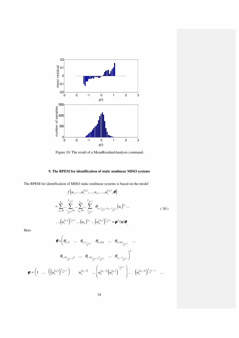
8.2 Mean residual analysis

Mean residual analysis is a method that evaluates the obtained static characteristics of an identified

model of any kind. It operates by sorting residual errors into bins, the bin being decided by the value

of the measured output signal with the same time index as the residual error. The mean of the residuals

are then computed, in each bin, and plotted against the range of the output signal. The number of

samples of each bin is also plotted. The user is referred to [ 7 ] for further details. In order to perform

mean residual analysis, the user is required to

1. Execute the script MeanResidualAnalysis.m.

2. Provide the intervals used by the method when prompted for intervals.

Example 16: This example performs mean residual analysis using about 40 intervals, each with an

output amplitude width of 0.1. The MATLAB command window command is

» meanResidualAnalysis

ans =

Input intervals for division into bins

K» intervals=(-2:0.1:2);

K» return

»

The following plot results

34

Figure 10: The result of a MeanResidualAnalysis command.

9. The RPEM for identification of static nonlinear MISO systems

The RPEM for identification of MISO static nonlinear systems is based on the model

( ) ( )( )f u u u un

k k

nk

1 11, ... , , ... , , ... , ,θθθθ

( )

( )

====

∑∑∑ ... ... ...i

I

i

I

i

I

uk

uk

un

un

u

u

000

11

11

1

1

( )

( )

i

I

uk

nk

uk

nk

∑( ) ( )

( )θi i i i

i

uu

n ukuk

nk

u

u1

11

1

1... ... .... ...

( )( ) ( ) ( ) ( )( ) ( ).. . . .. .. .u u u

ni

k

i

k

ni

un uk k u

k

nk

11

11

= ( )ϕϕϕϕ θθθθT u.

( 30 )

Here

θθθθ =( ) ( )

θ θ θ θ0 0 0 0 010 0 01... ... ... ...... ... ...I Iu

k

nku

k

nk

( ) ( ) ( ) ( )θ θ θ0 0 0 0 0

1 1 1... ... ...... ...I I I I I

T

uknk uk

nk uknk u

uknk− −

ϕϕϕϕ = ( )( ) ( ) ( )1

1... ...u uk

nI

k

nk uk

nk k

− ( ) ( )( )

( )

u uk

n

k

nk k

I

uk

nk

−

1 ( )( ) ( )... ...uk

nI

k uk

nk− −1 1

-3 -2 -1 0 1 2 3-0.2

-0.1

0

0.1

0.2

y(1)

me

an

re

sid

ua

l

-3 -2 -1 0 1 2 30

500

1000

1500

y(1)

nu

mb

er

of

sa

mp

les

35

( )( ) ( ) ( )( ) ( )u uk

nI

k

nI

k uk

nk k uk

nk− −

1 1

... ( ) ( )( ) ( )u u

I

k

nI

Tu

k uk

nk

1

1...

.

(31)

The recursive algorithm is then developed exactly as in [1] and [2]. The main difference is that the

state equation iteration and the corresponding state gradient iteration disappears. The end result is the

following algorithm where all variables are explained in detail in [1] and [2]

( ) ( ) ( )εεεε t t tm= −y y

( ) ( )ΛΛΛΛ ΛΛΛΛt t TS= − +( )µ t

t( ) ( ) ( )( )εεεε εεεεt t t T

TS− −ΛΛΛΛ

( ) ( )R Rt t TS= − +( )µ t

t( ) ( ) ( ) ( )( )ψψψψ ψψψψt t t t T

TSΛΛΛΛ− − −1

R

( ) ( )[$ $θθθθ θθθθt t TS= − +( )µ t

t( ) ( ) ( ) ( )]R − −1 1t t t tψψψψ εεεεΛΛΛΛ

( ) ( ) ( )( ) ( ) ( ) ( ) ( ) ( )( ) ( ) ( )( )( )

ϕϕϕϕ t u t u t u t u tk

nI

k

n

k

n

k

nk uk

nk k k k

I

uk

nk

=

− −1

1 1. . . . .. .. .

( ) ( )( ) ( ) ( ) ( )( ) ( ) ( ) ( )( ) ( ) ( )( ) ( ) ( )( ) ( )... ... ... ...u t u t u t u t u tk

nI

k

nI

k

nI I

k

nI

T

k uk

nk k uk

nk k uk

nk u k uk

nk− −− −

1 1

1

1 11

( ) ( )y t T tS

T+ = ϕϕϕϕ θθθθ

( ) ( )ψψψψ ϕϕϕϕt T t TS s+ = + .

( 32 )

It should be noted that this algorithm collapses to a least-squares case. Hence it will always converge.

10. Software – Static case

All software for identification of nonlinear static systems fits into the framework of Figure 1. As much

as possible of the software has been kept usable for both the nonlinear dynamic case and the nonlinear

static case. However, static versions of the following 7 scripts replace or add to the dynamic

counterparts, in case a static model is identified: dhdthetaStatic_m.m (new m-file),

GenerateDataStatic.m, hStatic_m.m, RPEMStatic.m, SetupDataStatic.m, SetupRPEMStatic.m

and SimulateModelOutputstatic.m. These files are now briefly described.

SetupDataStatic.m: This m-file sets up the parameters needed for static data generation. The file has

been modified by selection of parameters needed for dynamic data generation consistent with the static

case. Most variables are however left as dummy variables, so that SetupDataStatic.m does not

prevent the successful execution of existing scripts later in the data processing chain.

36

GenerateDataStatic.m: This file has been created from GenerateData.m by deletion of the state

iteration. Note that this script makes use of h.m that must be based only on input signals in the static

case. The state argument in the call is an empty matrix.

SetupRPEMStatic.m: This file has been created from SetupRPEM.m by setting the state dimension

equal to zero, by setting state initial values equal to a 0x1 matrix, and by setting the sampling period

scale factor scalingTs equal to 1. The latter is important since no scaling shall be applied in the static

case.

RPEMStatic.m: This file has been created from RPEM.m by deletion of the parts of the algorithm

that are not relevant in the static case. This is true for the state variable iteration and the corresponding

state gradient iteration. The exact details follow by a comparison of the RPEM of [2] with (32) above.

A further modification is the use of calls to the functions hStatic_m.m and dhdthetaStatic_m.m, in

order to compute output predictions and gradients.

hStatic_m.m: This function computes (30) above. It was created by small modifications of f_m.m.

The order of the output prediction (1) is e.g. included in the function call.

DhdthetaStatic_m.m: This function generates ϕϕϕϕ of (31). It was cretaed by small modifications of

dfdtheta_m.m. The order of the output prediction (1) is e.g. included in the function call.

SimulateModelOutputStatic.m. This file has been created from SimulateModelOutput.m by

deletion of the state variable iteration and by a call to the function hStatic_m.m for computation of the

output prediction.

11. Kalman filter based initialization algorithm

The Kalman filter based algorithm for initialization of the RPEM (dynamic case) is based on (3) just

like the RPEM. The recursive algorithm is then developed exactly as in [ 5 ] and [ 6 ]. The end result is

the following scheme where all variables are explained in detail in [ 5 ] and [ 6 ]

Initiate

)|0(),|0( SS TPTx −−

Iterate

1

2 ))|(()|()( −+−−= RHTttHPHTttPtKT

S

T

S

))|()()(()|()|( SmS TttxHtytKTttxttx −−+−=

)|()()|()|( SS TttHPtKTttPttP −−−=

)())(),(,()|( txtuttFtTtx S ξ=+

( 33 )

37

1))(),(,()|())(),(,()|( RtuttFttPtuttFtTtPT

S +=+ ξξ

It should be noted that this algorithm is similar to a least squares problem, solved recursively. Hence

(33) will always converge. The key ides to obtain the algorithm is to replace the estimated states of the

RPEM by an approximation ( )ξ t , obtained by repeated differentiation of the output signal. Note that

the scaled sampling period needs to be applied in the preceeding differentiation step, cf. [ 5 ] and [ 6 ].

12. Software – Kalman filter based initialization algorithm

To use the Kalman filter based initialization algorithm the following steps are required. Please note,

that since this algorithm is based on the same model structure as the dynamic RPEM in section 6 some

of the information is identical.

12.1 Initialization setup

The preparation for the identification run requires that the user

1. Modifies the output equation and the corresponding derivative of the underlying ODE model, as

given by h_m.m and dhdx_m.m. The function h_m.m implements the output equation of the

model. Note that this function is allowed to be a nonlinear function of the state and input. The

function is not allowed to be dependent on the estimated parameters, it must be known a priori.

Note also that the derivative of the function, with respect to the estimated state, needs to be

supplied in the function dhdx_m.m.

2. Provides further input data in the script SetupInit.m. The parameters that define the data

generation are directly written into this script. These parameters define the dimension of the

system, the initial value used in the ODE model, the size of the initial value of the P -recursion of

(33), the magnitude of the covariance matrices for the state and parameter vector system

disturbances, ( xR ,1 and θ,1R respectively), the magnitude of the measurement noise covariance,

2R , the scale factor, as well as the down-sampling period used to avoid too large logs during long

runs with high degree models. The reader is referred to [ 1 ] - [ 6 ] for details on these parameters,

as well as on their use.

3. Executes SetupInit.m. This loads the necessary parameters into the MATLAB workspace.

Example 17: The system used above is to be identified with a second order model, which implies

that the true parameter and corresponding regressor vectors are

( )T00120110 −−−=θ

( ) ( )ϕϕϕϕ x,u u x x u x x u x x x x uT

= 1 2 2 1 1 1 2 1 2 .

( 34 )

( 35 )

38

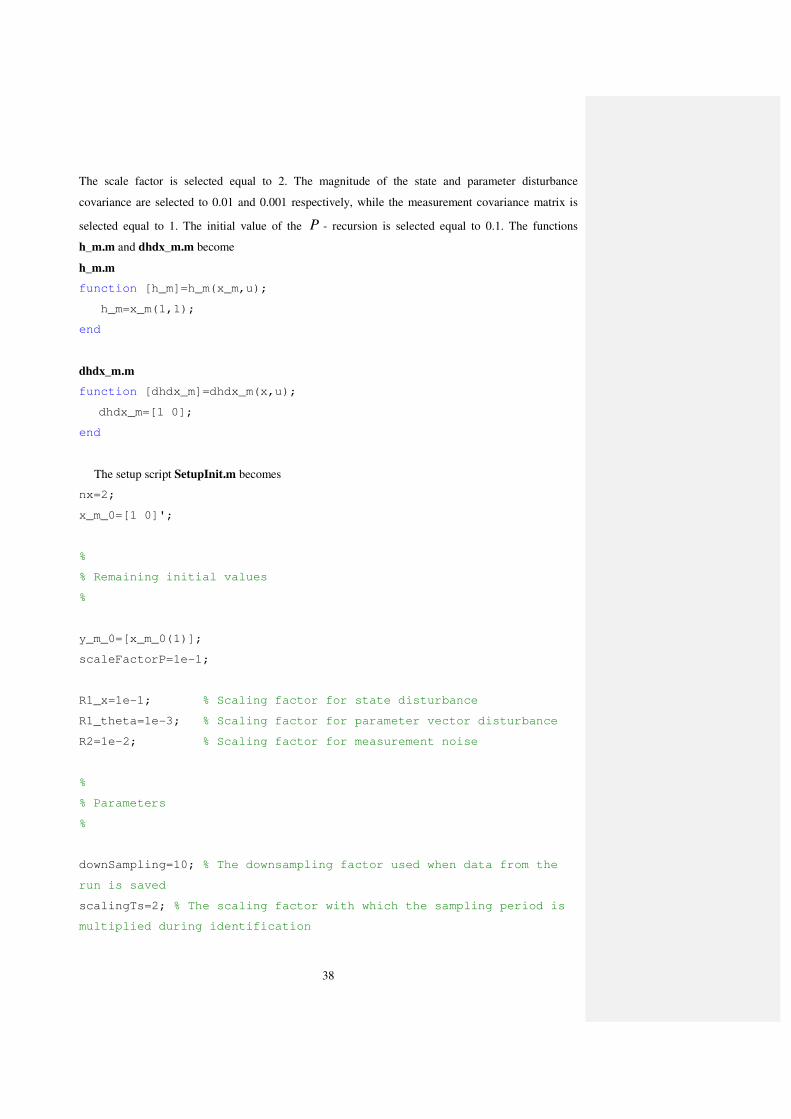
The scale factor is selected equal to 2. The magnitude of the state and parameter disturbance

covariance are selected to 0.01 and 0.001 respectively, while the measurement covariance matrix is

selected equal to 1. The initial value of the P - recursion is selected equal to 0.1. The functions

h_m.m and dhdx_m.m become

h_m.m

function [h_m]=h_m(x_m,u);

h_m=x_m(1,1);

end

dhdx_m.m

function [dhdx_m]=dhdx_m(x,u);

dhdx_m=[1 0];

end

The setup script SetupInit.m becomes

nx=2;

x_m_0=[1 0]';

%

% Remaining initial values

%

y_m_0=[x_m_0(1)];

scaleFactorP=1e-1;

R1_x=1e-1; % Scaling factor for state disturbance

R1_theta=1e-3; % Scaling factor for parameter vector disturbance

R2=1e-2; % Scaling factor for measurement noise

%

% Parameters

%

downSampling=10; % The downsampling factor used when data from the

run is saved

scalingTs=2; % The scaling factor with which the sampling period is

multiplied during identification

39

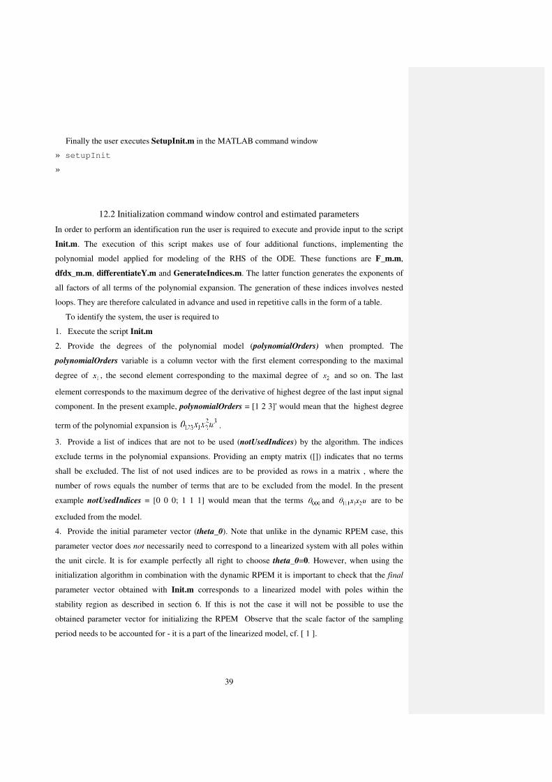
Finally the user executes SetupInit.m in the MATLAB command window

» setupInit

»

12.2 Initialization command window control and estimated parameters

In order to perform an identification run the user is required to execute and provide input to the script

Init.m. The execution of this script makes use of four additional functions, implementing the

polynomial model applied for modeling of the RHS of the ODE. These functions are F_m.m,

dfdx_m.m, differentiateY.m and GenerateIndices.m. The latter function generates the exponents of

all factors of all terms of the polynomial expansion. The generation of these indices involves nested

loops. They are therefore calculated in advance and used in repetitive calls in the form of a table.

To identify the system, the user is required to

1. Execute the script Init.m

2. Provide the degrees of the polynomial model (polynomialOrders) when prompted. The

polynomialOrders variable is a column vector with the first element corresponding to the maximal

degree of , the second element corresponding to the maximal degree of and so on. The last

element corresponds to the maximum degree of the derivative of highest degree of the last input signal

component. In the present example, polynomialOrders = [1 2 3]' would mean that the highest degree

term of the polynomial expansion is .

3. Provide a list of indices that are not to be used (notUsedIndices) by the algorithm. The indices

exclude terms in the polynomial expansions. Providing an empty matrix ([]) indicates that no terms

shall be excluded. The list of not used indices are to be provided as rows in a matrix , where the

number of rows equals the number of terms that are to be excluded from the model. In the present

example notUsedIndices = [0 0 0; 1 1 1] would mean that the terms and are to be

excluded from the model.

4. Provide the initial parameter vector (theta_0). Note that unlike in the dynamic RPEM case, this

parameter vector does not necessarily need to correspond to a linearized system with all poles within

the unit circle. It is for example perfectly all right to choose theta_0=0. However, when using the

initialization algorithm in combination with the dynamic RPEM it is important to check that the final

parameter vector obtained with Init.m corresponds to a linearized model with poles within the

stability region as described in section 6. If this is not the case it will not be possible to use the

obtained parameter vector for initializing the RPEM Observe that the scale factor of the sampling

period needs to be accounted for - it is a part of the linearized model, cf. [ 1 ].

40

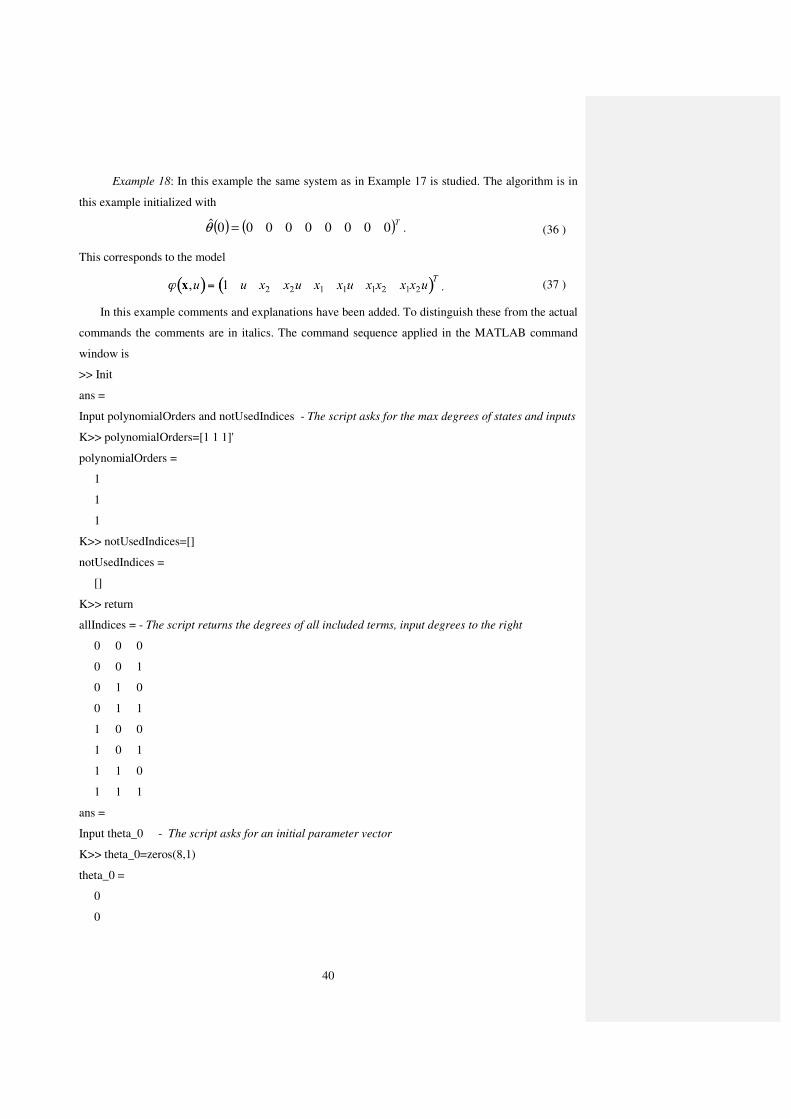
Example 18: In this example the same system as in Example 17 is studied. The algorithm is in

this example initialized with

( ) ( )T000000000ˆ =θ . (36 )

This corresponds to the model

. (37 )

In this example comments and explanations have been added. To distinguish these from the actual

commands the comments are in italics. The command sequence applied in the MATLAB command

window is

>> Init

ans =

Input polynomialOrders and notUsedIndices - The script asks for the max degrees of states and inputs

K>> polynomialOrders=[1 1 1]'

polynomialOrders =

1

1

1

K>> notUsedIndices=[]

notUsedIndices =

[]

K>> return

allIndices = - The script returns the degrees of all included terms, input degrees to the right

0 0 0

0 0 1

0 1 0

0 1 1

1 0 0

1 0 1

1 1 0

1 1 1

ans =

Input theta_0 - The script asks for an initial parameter vector

K>> theta_0=zeros(8,1)

theta_0 =

0

0

41

0

0

0

0

0

0

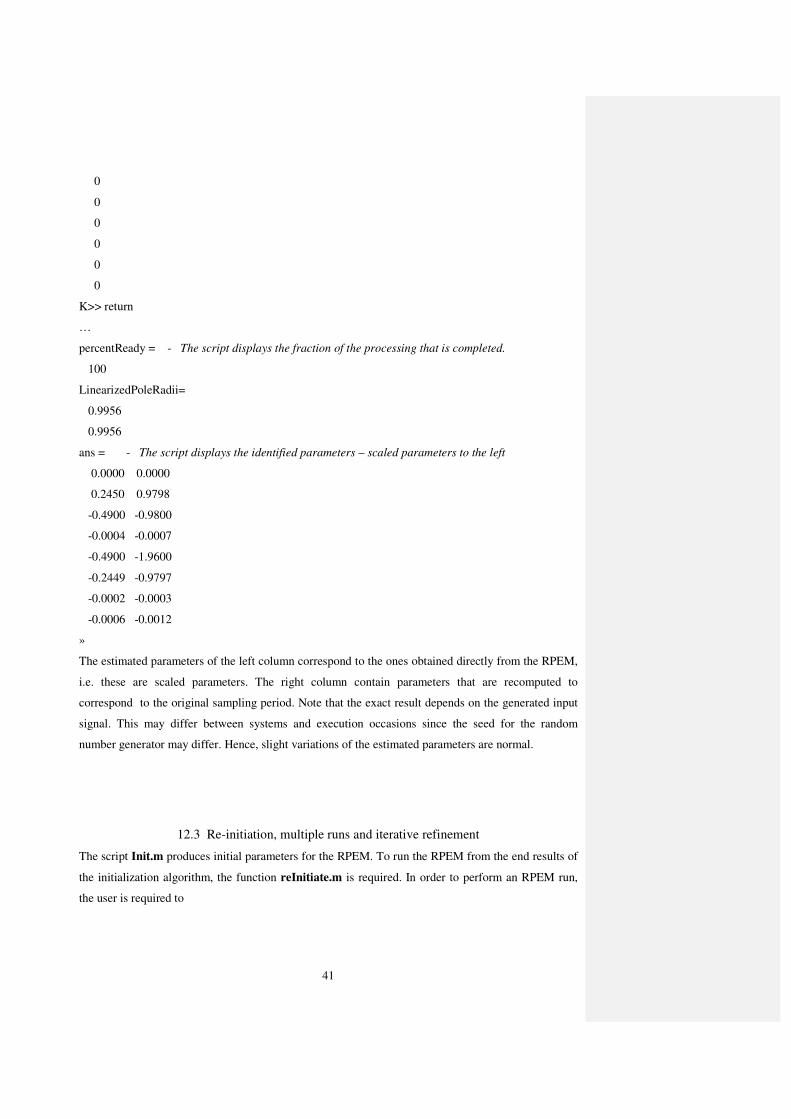
K>> return

…

percentReady = - The script displays the fraction of the processing that is completed.

100

LinearizedPoleRadii=

0.9956

0.9956

ans = - The script displays the identified parameters – scaled parameters to the left

0.0000 0.0000

0.2450 0.9798

-0.4900 -0.9800

-0.0004 -0.0007

-0.4900 -1.9600

-0.2449 -0.9797

-0.0002 -0.0003

-0.0006 -0.0012

»

The estimated parameters of the left column correspond to the ones obtained directly from the RPEM,

i.e. these are scaled parameters. The right column contain parameters that are recomputed to

correspond to the original sampling period. Note that the exact result depends on the generated input

signal. This may differ between systems and execution occasions since the seed for the random

number generator may differ. Hence, slight variations of the estimated parameters are normal.

12.3 Re-initiation, multiple runs and iterative refinement

The script Init.m produces initial parameters for the RPEM. To run the RPEM from the end results of

the initialization algorithm, the function reInitiate.m is required. In order to perform an RPEM run,

the user is required to

42

1. Run the script reInitiate.m. That script prompts the user for polynomialOrders and

notUsedIndices. The parameter vector at the end of the run, together with the previous and new

degrees, are then used to re-initiate all relevant quantities of the RPEM.

2. Run the SetupRPEM.m file, as described in section 6.

3. Rerun RPEM.m. Note that the RPEM does not need to prompt the user for any further information

this time.

Here, reinitiate.m is used in exactly the same way as described in section 6.3. Note, however, that the

model structure is normally not changed when the initialization algorithm is used in combination with

the RPEM, as the initial parameters are given for a specific model structure. By changing the model

structure between the initialization and RPEM algorithms, the benefits of an initialization algorithm

may be lost or significantly reduced.

13. Summary

This report describes a software package for identification of nonlinear systems. Future work in this

field, that result in useful MATLAB routines, will be integrated with the presently available

functionality. Updated versions of this report will then be made available.

14. References

[ 1 ] T. Wigren, "Recursive Prediction Error Identification of Nonlinear State Space Models",

Technical Reports from the department of Information Technology 004-2004, Uppsala University,

Uppsala, Sweden, January, 2004.

[ 2 ] T. Wigren, "Recursive prediction error identification and scaling of nonlinear state space models

using a restricted black box parameterization", Automatica, vol. 42, no. 1, pp. 159-168, 2006.

[ 3 ] T. Wigren "Scaling of the sampling period in nonlinear system identification", in Proceedings of

IEEE ACC 2005, Portland, Oregon, U.S.A., pp. 5058-5065, June 8-10, 2005.

[ 4 ] T . Wigren "Recursive identification based on nonlinear state space models applied to drum-

boiler dynamics with nonlinear output equations", in Proceedings of IEEE ACC 2005, Portland,

Oregon, U.S.A., pp. 5066-5072, June 8-10, 2005.

[5] L. Brus, Nonlinear Identification and Control with Solar Energy Applications. Ph. D. Dissertation,

Department of Information Technology, April 25, 2008.

[ 6 ] L. Brus, T. Wigren and B. Carlsson "Initialization of a nonlinear identification algorithm applied

to laboratory plant data", to appear in IEEE Trans. Contr. Sys. Tech., 2008.

43

[ 7 ] D. Hanselmann and B. Littlefield. Mastering Matlab 5 - A Comprehensive Tutorial and

Reference. Upper Saddle River, NJ: Prentice Hall, 1998.

[ 8 ] L. Ljung and T. Söderström. Theory and Practice of Recursive Identification. Cambridge, Ma:

MIT Press, 1983.

[ 9 ] T. Wigren, "User choices and model validation in system identification using nonlinear Wiener

models", Prep. 13:th IFAC Symposium on System Identification , Rotterdam, The Netherlands, pp.

863-868, August 27-29, 2003. Invited session paper.

[ 10 ] T. Wigren, “MATLAB software for recursive identification and scaling using a structured

nonlinear black—box model – revision 1”, Technical Reports from the department of Information

Technology 2005-002, Uppsala University, Uppsala, Sweden, January, 2005.

[ 11 ] T. Wigren, “MATLAB software for recursive identification and scaling using a structured

nonlinear black—box model – revision 2”, Technical Reports from the department of Information

Technology 2005-022, Uppsala University, Uppsala, Sweden, August, 2005.

[ 12 ] S. Tayamon and T. Wigren “Recursive Prediction Error Identification and Scaling of Non-linear

Systems with Midpoint Numerical Integration”, Technical Reports from the department of Information

Technology, In preparation, Uppsala University, Uppsala, Sweden, September, 2010.

Formaterat: Svenska (Sverige)

MATLAB Software for Recursive Identification and … · 1 MATLAB Software for Recursive...

Documents

Transcript of MATLAB Software for Recursive Identification and … · 1 MATLAB Software for Recursive...