Matlab Notes for Differential Equations

Lia Vas

Content 1. M-files2. Basics of first order differential equations3. Direction field4. Numerical solutions using ode45 5. Euler method

Practice problems 16. Second and higher order differential equations

Practice problems 27. Systems of differential equations

1. M-files

Suppose that you want to perform the same operation many times for different input values.Matlab allows you to create a function or a script that you can execute repeatedly withdifferent input values (i.e. to do programming). Such function or a script is called an M-file. AnM-file is an ordinary text file containing Matlab commands. You can create them using anytext editor that can save files as plain (ASCII) text. You can also create an M-file by using“File” menu and choosing “New M-file” option from your Matlab command window. Animportant fact to keep in mind when using M-files is that an M-file can be executed from thecommand window just if the "Current Directory" on the top of the command window is set tobe the same directory where the M-file is saved.

Example 1.1. Suppose that you want to solve the equation ax² + bx + c = 0 using thequadratic formula. We can create a function which will have as input values of a, b and c andwhich will give the solution(s) of the quadratic equation. We can enter the following in an M-file. function [x1 x2] = quadratic1(a, b, c)x1 = (-b+sqrt(b^2-4*a*c))/(2*a);x2 = (-b-sqrt(b^2-4*a*c))/(2*a);

To execute the M-file and find solutions of x² -3x + 2 = 0, you can use >> [x1, x2] = quadratic(1, -3, 2)The output is x1 = 2 x2 = 1Note that the semi-colon symbol after the commands suppresses display of the results ofthese commands. The values of x1 and x2 will still be displayed since we listed thesevariables in the brackets of the function.

Alternatively, the following M-file can be used. function [ ] = quadratic2(a, b, c)

- 1 -

x1 = (-b+sqrt(b^2-4*a*c))/(2*a)x2 = (-b-sqrt(b^2-4*a*c))/(2*a)Here we do not need to list the variables in the first line since we did not use the semi-colonsymbols when computing the values of x1 and x2. Also, you do not need to list x1 and x2 inthe first line since they will be displayed when 2nd and 3rd lines are executed. Also, you canexecute this M-file to solve x² -3x + 2 = 0 simply as quadratic(1, -3, 2) instead of [x1, x2] =quadratic(1, -3, 2) The output is the same as for the first version. >> quadratic(1, -3, 2)This means that you want to solve the equation. Matlab gives you the answers: x1 = 2 x2 = 1These M-files produce the complex values if the solutions of a quadratic equation arecomplex numbers. For example, to solve x² + 4 = 0, we can use >> quadratic(1, 0, 4)x1 = 0 + 2.0000i x2 = 0 - 2.0000i

Example 1.2. Suppose that we need to write a program that calculates the Cartesian coordinates (x,y) of a point given by polar coordinates (r,θ). One possible solution is the following M-file. function [x, y] = polar(r, theta)x = r*cos(theta);y = r*sin(theta);

For example, to calculate (x,y) coordinates of for r=3 and θ = π , we can use the command [x,y]=polar(3, pi) and get the answer x = -3 y = 3.6739e-016Note that y is very close to 0. The inaccuracy comes from the fact that using pi for π in Matlabgives an approximation of π not the exact value. The exact representation of π is obtained bysym('pi'). The command [x,y]=polar(3, sym('pi')) gives you the expected answer x = -3 y = 0.

2. Basics of First Order Differential Equations

To find symbolic solution of a differential equation, you can use the command dsolve. To usedsolve, the derivative of the function y is represented by Dy. The command has the followingform:

dsolve('equation', 'independent variable')

If we have the initial condition, we can get the particular solution on the following way:

dsolve('equation', 'initial condition', 'independent variable')

Example 2.1. Consider the equation x y' - y = 1. a) Find the general solution. b) Find theparticular solution corresponding to the initial condition y(1)=5 and graph it.

a) You can find the general solution by using: >> dsolve('x*Dy-y=1', 'x') You obtain ans = -1+x*C1 This means that the solution is any function of the form y = -1+

- 2 -

cx, where c is any constant.

b) To find the solution of x y' - y = 1 with the initial condition y(1)=5, we can use:>> dsolve('x*Dy-y=1', 'y(1)=5', 'x') ans = -1+6*xTo graph this solution, we can use: >> ezplot(ans)

We can graph a couple of different solutions on the same chart.

Example 2.2. Graph the solutions of the equation y' = x+y for y(0) taking integer valuesbetween -2 and 4.

First we can find the solution with the initial condition of the form y(0)=c. >> s = dsolve('Dy = x+y', 'y(0)=c', 'x') s = -x-1+exp(x)*(1+c)

Then, we can use the following M-file to produce the graph of the required particularsolutions.

function[ ]=many_solutions(s)for cval=-2:1:4 (this means that the variable cval is taking values starting at -2 and

ending at 4 with step size of 1. Change this line if you need to use different values of c)

hold on ezplot(subs(s, 'c', cval)) (this means that the value of c in s is substituted by values of

cval. Add the domain of the solutions to this command as explained in Review of Matlab if necessary)

hold offend

You can execute the M-file by >> many_solutions(s)

You can modify the window by using thecommand

axis([xmin, xmax, ymin, ymax])

For example, in the previous example you canuse axis([-1 6, -100 100]).

By changing s and values of c, you canmodify the M-file to produce graphs ofsolutions of different equations as the nextexample illustrates.

Example 2.3. Let us graph the solutions ofthe equation y' = (y-2)(100-y) for sufficiently many values of y(0) so that the limiting behaviorof all solutions can be determined.

- 3 -

First we solve the equation naming the general solution s. >> s = dsolve('Dy = (y-2)*(100-y)', 'y(0)=c', 'x') Since this is an autonomous equation with the equilibrium solutions at y=2 and y=100, inorder to get a telling graph, we can graph a few solutions with initial conditions less than 2, afew between 2 and 100 and a few above 100. We can use the same M-file as in the previousexample, but with a few modification. For one, we need to modify the line that specifies thevalues of initial condition c. For example we can take the values of c to be 0, 10, 20, ... , 150.So, we start at 0 and end with 150 making the step size of 10. In Matlab, we can representthis by 0:10:150. Thus, substitute the line cval=-2:1:4 with cval=0:10:150 and use the M-filemany_solutions again. Secondly, to see the graphs for t values larger than 6, [0, 15] forexample, modify the line with ezplot to be ezplot(subs(s, 'c', cval), [0 15]). Finally, a nicewindow for this graph can be axis([0 15 0 150]) for example.

3. Direction Fields

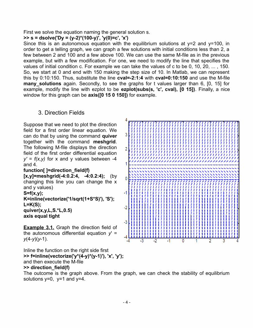
Suppose that we need to plot the directionfield for a first order linear equation. Wecan do that by using the command quivertogether with the command meshgrid.The following M-file displays the directionfield of the first order differential equationy' = f(x,y) for x and y values between -4and 4. function[ ]=direction_field(f)[x,y]=meshgrid(-4:0.2:4, -4:0.2:4); (bychanging this line you can change the xand y values)S=f(x,y);K=inline(vectorize('1/sqrt(1+S*S)'), 'S');L=K(S);quiver(x,y,L,S.*L,0.5)axis equal tight

Example 3.1. Graph the direction field ofthe autonomous differential equation y' =y(4-y)(y-1).

Inline the function on the right side first >> f=inline(vectorize('y*(4-y)*(y-1)'), 'x', 'y'); and then execute the M-file>> direction_field(f)The outcome is the graph above. From the graph, we can check the stability of equilibriumsolutions y=0, y=1 and y=4.

- 4 -

4. Numerical solutions using ode45

Many differential equations cannot be solved explicitly in terms of elementary functions. forthose equations, approximate solutions can be obtained using numerical methods.Approximate solutions can be found by using the command ode45. We can illustrate the useof this command on the following example.

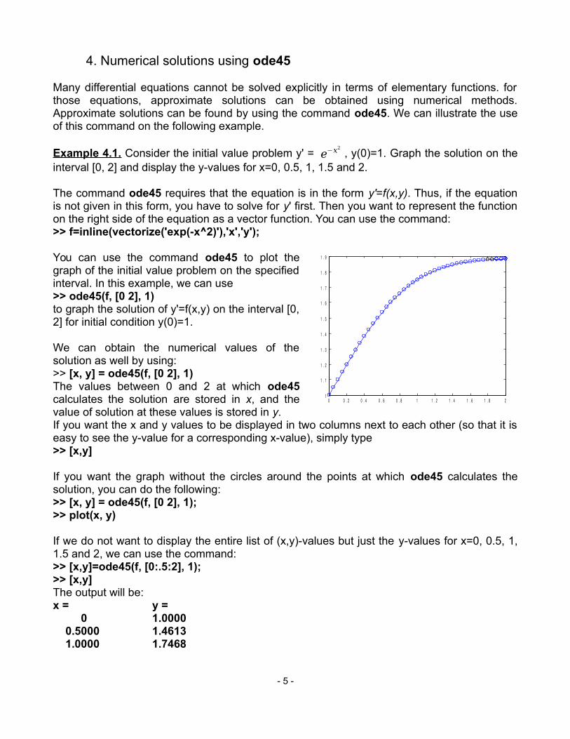
Example 4.1. Consider the initial value problem y' = e−x2 , y(0)=1. Graph the solution on theinterval [0, 2] and display the y-values for x=0, 0.5, 1, 1.5 and 2.

The command ode45 requires that the equation is in the form y'=f(x,y). Thus, if the equationis not given in this form, you have to solve for y' first. Then you want to represent the functionon the right side of the equation as a vector function. You can use the command: >> f=inline(vectorize('exp(-x^2)'),'x','y');

You can use the command ode45 to plot thegraph of the initial value problem on the specifiedinterval. In this example, we can use >> ode45(f, [0 2], 1)to graph the solution of y'=f(x,y) on the interval [0,2] for initial condition y(0)=1.

We can obtain the numerical values of thesolution as well by using: >> [x, y] = ode45(f, [0 2], 1)The values between 0 and 2 at which ode45calculates the solution are stored in x, and thevalue of solution at these values is stored in y. If you want the x and y values to be displayed in two columns next to each other (so that it iseasy to see the y-value for a corresponding x-value), simply type >> [x,y]

If you want the graph without the circles around the points at which ode45 calculates thesolution, you can do the following: >> [x, y] = ode45(f, [0 2], 1);>> plot(x, y)

If we do not want to display the entire list of (x,y)-values but just the y-values for x=0, 0.5, 1,1.5 and 2, we can use the command:>> [x,y]=ode45(f, [0:.5:2], 1);>> [x,y]The output will be: x = y = 0 1.0000 0.5000 1.4613 1.0000 1.7468

- 5 -

0 0 . 2 0 . 4 0 . 6 0 . 8 1 1 . 2 1 . 4 1 . 6 1 . 8 21

1 . 1

1 . 2

1 . 3

1 . 4

1 . 5

1 . 6

1 . 7

1 . 8

1 . 9

1.5000 1.8562 2.0000 1.8821

5. Euler Method

The following M-file calculates the numerical values of the solution of an initial value problemusing the Euler method. It approximates the solution of the initial value problem y' = f(x,y),y(x0) = y0 on the interval [x0, xn] using n steps using the following formulas:

h = (xn - x0)/n, xi+1 = xi +h, and yi+1 = yi +f(xi , yi) h

for all i=0,1...,n-1. The input is the inline function f, x0, y0, xn and n. The output is the list of xand y values of the approximate solution.

function [x, y] = euler(f, xinit, yinit, xfinal, n)h = (xfinal - xinit)/n; (calculates the step size)x = zeros(n+1, 1);y = zeros(n+1, 1); (initialize x and y as column vectors of size n+1)x(1) = xinit;y(1) = yinit; (the first entry in the vectors x and y is x0 and y0 respectively)for i = 1:n x(i + 1) = x(i) + h; (every entry in vector x is the previous entry plus the step size h) y(i + 1) = y(i) + h*f(x(i), y(i)); (Euler Method formula)end

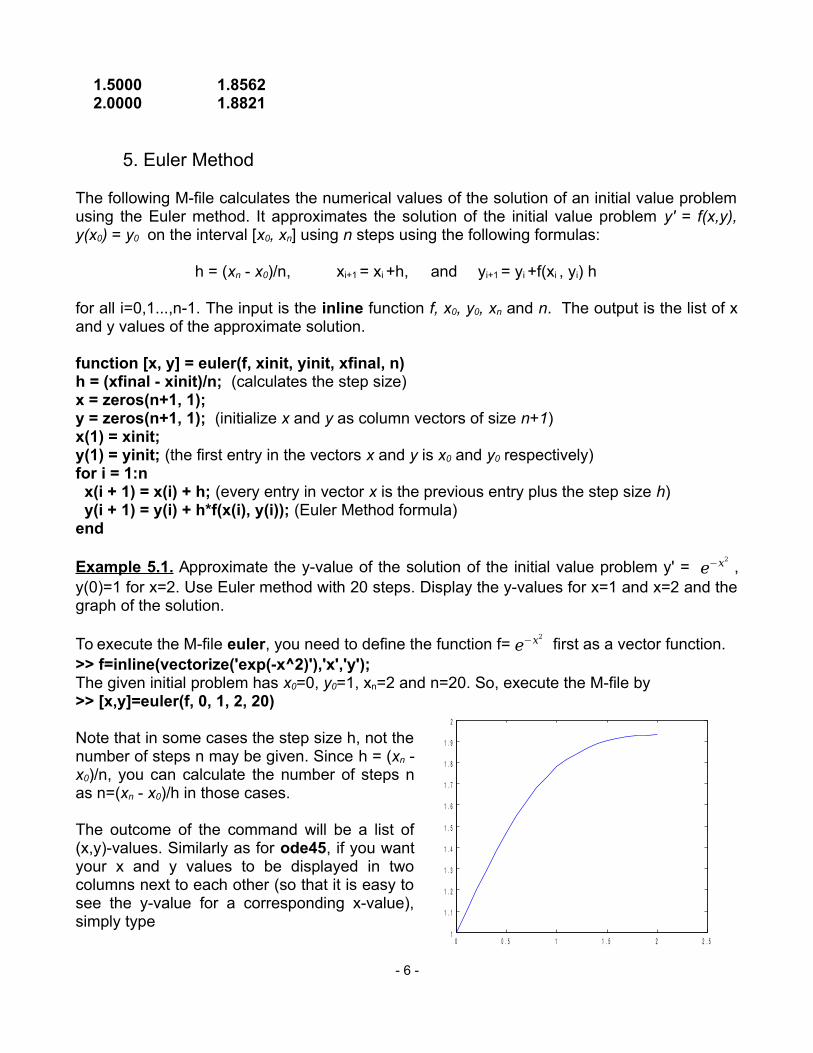
Example 5.1. Approximate the y-value of the solution of the initial value problem y' = e−x2 ,y(0)=1 for x=2. Use Euler method with 20 steps. Display the y-values for x=1 and x=2 and thegraph of the solution.

To execute the M-file euler, you need to define the function f= e−x2 first as a vector function. >> f=inline(vectorize('exp(-x^2)'),'x','y');The given initial problem has x0=0, y0=1, xn=2 and n=20. So, execute the M-file by >> [x,y]=euler(f, 0, 1, 2, 20)

Note that in some cases the step size h, not thenumber of steps n may be given. Since h = (xn -x0)/n, you can calculate the number of steps nas n=(xn - x0)/h in those cases.

The outcome of the command will be a list of(x,y)-values. Similarly as for ode45, if you wantyour x and y values to be displayed in twocolumns next to each other (so that it is easy tosee the y-value for a corresponding x-value),simply type

- 6 -

0 0 . 5 1 1 . 5 2 2 . 51

1 . 1

1 . 2

1 . 3

1 . 4

1 . 5

1 . 6

1 . 7

1 . 8

1 . 9

2

>> [x,y]To graph this list, use plot(x,y).

The list consists of 21 (x,y) points. The list starts with the initial condition (x,y)=(0,1). The x-values are all h=(2-0)/20=0.1 units apart. The last x-value is 2 and the corresponding y-valueis 1.9311. From this list you can see the y-values corresponding to x=1 and x=2.

x y1 1.77782 1.9311

Alternatively, if you need to display a specific (x,y)-value, you need to determine the i-valuethat corresponds to this point (i.e. you need to count the steps performed until the point hasbeen calculated). Then you can display the point by typing x(i) and y(i).

For example, the point with x=1 is the 11th point calculated (Note: not 10th point - recall thatx=0 corresponds to first point calculated, not the zeroth point calculated). So, to display this x-value you can type>> x(11) and obtain the answer ans = 1.000To display the corresponding y-value, you can type >> y(11) and obtain the answer ans = 1.7778Similarly, the point with x=2 is the 21th point calculated. You can display the x and y values asfollows. >> x(21) ans = 2.000>> y(21) ans = 1.9311

Practice problems

1. a) Find the general solution of the differential equation y'-2y=6x. b) Find the particular solution with initial condition y(0)=3.c) Plot the particular solution on interval [0,2] and find the value of this solution at 2.

2. Graph the solutions of the differential equation y'=0.1y(1-y) for the y-values of the initialcondition y(0) taking values 0.1, 0.3, 0.5 and 0.7.

3. Consider the autonomous equation y' = (y+1)(3-y)²(5-y).a) Find the equilibrium solution(s) of the equation and check the stability. Sketch thegraph of all solutions.b) Use Matlab to sketch the direction field of this equation. Check if the graph agreeswith your answer for part a).

4. Consider the equation y' = (y+1)(3-y)²(5-y). Using ode45, find the value of the solutionwith the initial condition y(0)=4 at x=5. Graph the solution with initial condition y(0)=4for x-values in [0, 5].

5. Consider the equation y' = (y-1)(5-y). Using the M-file euler, find the value of thesolution with the initial condition y(0)=2 at x=3 for step size of 0.25. Graph the solution

- 7 -

with initial condition y(0)=2 for x-values in [0, 3].

Solutions. 1. a) General solution: dsolve('Dy-2*y=6*x', 'x') ans= (-6x-3)/2+C1*exp(2x)b) Particular solution: dsolve('Dy-2*y=6*x', 'y(0)=3', 'x') ans= (-6x-3+9*exp(2x))/2c) syms x ezplot((-6x-3+9*exp(2x))/2, [0 2])To find the value at 2: f=inline((-6x-3+9*exp(2x))/2, x) f(2)

ans=238.192. Modify the M-file many_solutions so thatthe second line is cval=0.1:0.2:0.7 (this meansthat cval is taking values starting at 0.1 andending at 0.7 that are 0.2 away from eachother). Thus cval= 0.1, 0.3, 0.5 and 0.7. Also, tosee better the limiting behavior of the solutions,you may want to graph the solutions on domainthat includes large values of x. To do thismodify the line with ezplot command toezplot(subs(s, 'c', cval), [0 100]) for example.Then execute s = dsolve('Dy=0.1*y*(1-y)','y(0)=c', 'x') and many_solutions(s) andobtain the following graph.

3. a) Set the right side of the equation equal to zero. Obtain theequilibrium solutions y=-1, y=3 and y=5. Analyze the sign. Obtainthat y=-1 is unstable, y=3 is semistable and y=5 is stable. b) First inline the function f=inline(vectorize('(y+1)*(3-y)^2*(5-y)'), 'x', 'y')

Then you can execute the relevant M-file by direction_field(f)To get a graph with all three equilibrium solutions displayed, youneed to modify the meshgrid command so that y-values smallerthan -1 and larger than 5 are displayed as well. For example,[x,y]=meshgrid(0:0.2:6, -3:0.2:10);

4. First, inline the function as a vector function using the samecommand as in previous problem. To display x andy values use [x,y]=ode45(f, [0,5], 4). The last y-value corresponds to value at x=5 and it isy=4.9997. To get the graph of solution with theinitial condition y(0)=4 on interval [0,5] use ode45(f,[0,5], 4).

5. First, inline the function as a vector function usingf=inline(vectorize('(y-1)*(5-y)'), 'x', 'y'). Note that thestep size of 0.25 corresponds to the number ofsteps n=(3-0)/0.25=12.

- 8 -

0 0.5 1 1.5 2 2.5 3 3.5 4 4.5 54

4.2

4.4

4.6

4.8

5

5.2

5.4

Execute the M-file euler by [x,y]=euler(f, 0, 2, 3, 12) To display the answers in two columns, one corresponding to x and the other to y-values usesimply [x,y]. The list starts by x=0 and y=2. The list ends with x=3 and y=5.000. Graph the listby using plot(x,y). The graph should look similar to the graph from the previous problem.

6. Second and Higher Order Differential Equations

Second order linear equations can be solved similarly as the first order differentialequations: analytically using dsolve and numerically using ode45. For command dsolve,recall that we represent the first derivative of the function y with Dy. The second derivative ofy is represented with D2y.

Example 6.1. a) Find general solution of y''-3y'+2y = sin x. b) Find the particular solution of the same equation with the initial conditions

y(0) = 1, y'(0)=-1.

a) For the general solution, use: >> dsolve('D2y-3*Dy+2*y=sin(x)', 'x')ans=3/10*cos(x)+1/10*sin(x)+C1*exp(x)+C2*exp(2*x)

b) For the particular solution with the initial conditions y(0) = 1, y'(0)=-1, use: >> dsolve('D2y-3*Dy+2*y=sin(x)', 'y(0)=1', 'Dy(0)=-1', 'x')ans = 3/10*cos(x)+1/10*sin(x)+5/2*exp(x)-9/5*exp(2*x).

For equations that can not be solved in terms of elementary functions, we usenumerical methods. For ode45, the second order differential equation must be converted toa system of two first order equations using the substitution

(S) y=y1 and y'=y2. The first equation of the new system reflects the relation between the two new functions: thesecond one is the derivative of the first. So, the first equation is

(1) y1'=y2 .The second equation is obtained by applying the substitution to the original differentialequation and solving it for y''=y2'. For example, the equation y''-3y'+2y = sin x from theprevious example with substitution (S) becomes y2'-3y2 +2 y1 = sin x. Solving for y2' producesthe second equation of the system to be y2'=sin x+3y2-2y1 . Thus, the system is

(1) y1'=y2 and (2) y2'=sin x+3y2-2y1

We illustrate the use of ode45 command for solving second order equations on the followingexample.

Example 6.2. Consider the following initial value problem

y'' + x y' + y = 0 with y(0)=1 and y'(0)=0.

(a) Using ode45, graph the solution on interval [0, 5]. (b) Using ode45, display the list of y-values of the solution for the integer x-values from 0 to 5.

- 9 -

First, you need to convert the given second order differential equation into a system of twofirst order equations using the substitution (S) y=y1 and y'=y2. The first equation of the newsystem is (1) y1'=y2 . The second equation is obtained by using the substitution for the givenequation y'' + xy' + y = 0 to obtain y2' + xy2+ y1 =0 and then solving for y2' to get (2) y2'=-xy2- y1.Thus, the newly obtained system is

(1) y1'=y2 and (2) y2'=-x y2- y1 .

In Matlab, the two new functions can be denoted by y(1) and y(2). The solution y will berepresented as vector y=[y(1); y(2)]. Keep in mind that y(1) corresponds to the solution y ofthe original equation. The function y(2) corresponds to the derivative y'. This problem is notasking for the derivative y' so you can consider y(2) to be a byproduct.

Inline the right side of the two equations as a vector function f that depends on independentvariable x and dependent variable y.

f=inline('[y(2); -x*y(2)-y(1)]','x','y');The first entry of f is the right side of the first equation and the second entry of f is the rightside of the second equation.

(a) To graph the solution on interval [0, 5], you canuse

ode45(f, [0, 5], [1;0])In this command, [0, 5] indicates the interval for xand [1;0] indicate the initial values y(0)=1 andy'(0)=0. The output is a graph with two functionsy(1) representing the solution y and y(2)representing its derivative y'. The first one will beplotted in blue and the second one in green.

Alternatively, you can use [x,y]=ode45(f, [0, 5], [1;0]); followed by plot(x,y)

The first command calculates numerical values ofthe solution. Since we do not need those valuesdisplayed, the command ends with a semi-colon.The second commands plots the valuescalculated. The graph looks similar as the firstgraph above.

To display graph of y without the graph of y', youcan use

[x,y]=ode45(f, [0, 5], [1;0]); followed byplot(x,y(:,1))

These command produce the following graph.

(b) To obtain numerical values of the solution use

[x, y] = ode45(f, [0:1:5], [1;0])Here [0:1:5] indicates that the x is taking values starting at 0, ending at 5 at step 1 away from

- 10 -

each other. [1;0] indicates the initial values, just as in part (a). The vector y in the output willconsist of two columns. The first y(1) consists of the values of the solution y at x-valuesbetween 0 and 5 and the second y(2) consists of the values of the derivative y' at thesepoints. If you want the x and y values to be displayed in columns next to each other (so that itis easy to see the y-value for a corresponding x-value), you can use [x,y]. Obtain the list

ans = 0 1.0000 0 1.0000 0.6065 -0.6065 2.0000 0.1354 -0.2707 3.0000 0.0111 -0.0333 4.0000 0.0003 -0.0013 5.0000 0.0000 -0.0000

Here the three columns represent x, y and y' values respectively.

Practice problems 21. a) Find the general solution of the equation y''-4 y'+4 y= ex +x². b) Find particular

solution of the initial value problem with y(0)=8, y'(0)=3.2. Using ode45 graph the solution of y'' + x² y' + y = cos 2x, y(0)=1, y'(0)=-1 for t in [0, 4].

Solutions

1. a) dsolve('D2y-4*Dy+4*y=exp(x)+x^2', 'x')ans = exp(x)+1/4*x^2+1/2*x+3/8+C1*exp(2*x)+C2*exp(2*x)*xb) dsolve('D2y-4*Dy+4*y=exp(x)+x^2','y(0)=8', 'Dy(0)=3', 'x')ans = exp(x)+1/4*x^2+1/2*x+3/8+53/8*exp(2*x)-47/4*exp(2*x)*x

2. Convert to a system using y=y1 and y'=y2. The first equation of the system is y1'=y2 and thesecond is obtained from y'' + x²y' + y = cos 2x → y2'+ x²y2 + y1 = cos 2x → y2'=cos 2x - x² y2 -y1. So the system is

(1) y1'=y2 and (2) y2'=cos 2x - x² y2 - y1

Inline the right side of the two equations as a vector function f by f=inline('[y(2); cos(2*x)-x^2*y(2)-y(1)]','x','y').

To graph the solution on interval [0, 4], you can use ode45(f, [0, 4], [1;-1]). The values [1;-1]correspond to the y and y' values from the initial conditions.

7. Systems of Differential Equations

Symbolic Solutions. You can find the symbolic solutions of a system of differential equationsby using the command dsolve.

Example 7.1. Consider the system dx/dt=2x-y dy/dt=3x-2y

a) Find the general solution of this system. b) Find the particular solution of the initial value problem with x(0)=1 and y(0)=2. c) Graph the particular solution on interval 0≤t≤20.

- 11 -

d) Plot sufficiently many solutions in the phase plane to determine the type of the equilibrium point (0,0).

a) [x,y] = dsolve('Dx = 2*x - y', 'Dy = 3*x - 2*y', 't')b) [x,y] = dsolve('Dx = 2*x - y', 'Dy = 3*x - 2*y', 'x(0) = 1', 'y(0) = 2', 't')c) To graph these two solutions on [0,20], you can use

ezplot(x, [0,20]) hold on ezplot(y, [0,20]) hold offd) To get the trajectories in the phase plane, you can graph a few solutions with different initialconditions on the same plot. For example, to graph the solutions for initial conditions x(0) and y(0) taking integer values between -2 and 2 and the value of parameter t between -3 and 3 taking 0.1 as a step size (thus, the t values will be: -3, -2.9, -2.8,...., 2.8, 2.9, 3) you can use the following M-file. close all; axes; hold on t = -3:0.1:3;for a = -2:2 for b = -2:2 echo off [x,y] = dsolve('Dx = 2*x - y', 'Dy =3*x - 2*y', 'x(0) = a', 'y(0) = b', 't');

xv = inline(vectorize(x), 't', 'a','b');

yv = inline(vectorize(y), 't', 'a','b'); plot(xv(t, a, b), yv(t, a, b)) endendhold offaxis([-10 10 -10 10])

From the graph, we conclude that(0,0) is unstable and that it is a saddle point.

Numeric Solutions. Finding symbolic solutions might be very limiting because many systemsof differential equations cannot be solved explicitly in terms of elementary functions. For thoseequations or systems of equations, numerical methods are used in order to get theapproximate solution. To find numeric solutions, you can use the command ode45. In order touse it, the system needs to be in the form x'=f(x,y,t) and y'=g(x,y,t) and the right sides of theequations should be represented as a vector function using inline first. The function x can berepresented as y(1) and the function y as y(2). The first entry of the inlined function f is theright side of the first equation and the second entry of f is the right side of the secondequation. Example 7.2. Consider the system

dx/dt=2x-x2-xy dy/dt=xy-ywith the initial conditions x(0)=1 and y(0)=2.a) Display the (x,y)-values of a numerical solution for t taking integer values between 0 and 6.

- 12 -

b) Graph the solutions on interval [0,20]. c) Graph the solution from b) in the phase plane. d) Plot sufficiently many solutions of this system (without the given initial conditions) in the phase plane to determine the type of the equilibrium point (1,1). First, inline the right side of equation as a function of independent variable t. The unknownfunctions x and y are represented by y(1) and y(2) respectively.

f = inline('[2*y(1)-y(1)^2-y(1)*y(2); y(1)*y(2)-y(2)]','t','y');

a) The command [t,y]=ode45(f, [0:1:6], [1;2])computes the (x,y)-values at t=0,1,2,...,6. The part [0:1:6] indicates that t-values start at 0, end at 6 and are 1 step away from each other. The part [1;2] reflects the initial conditions x(0)=1 and y(0)=2. Note that here y is a vector whose entries will be the values of y(1) representing x and y(2) representing y. If you want the t, x and y values to be displayed in columns next to each other (so that it is easy to see the (x,y)-value for a corresponding t-value), you can use [t,y]. Obtain the list

ans = 0 1.0000 2.0000 1.0000 0.5909 1.5148 2.0000 0.6791 1.0294 3.0000 0.9123 0.8370 4.0000 1.0763 0.8424 5.0000 1.0980 0.9281 6.0000 1.0502 1.0016

b) The command ode45(f,[0,20],[1;2]) will graph the two solutions on the same plot asfunctions of t. The function x will be graphed in blue and y in green (the first graph).

Alternatively, you can graph using [t,y]=ode45(f,[0 20],[1;2]); followed by plot(t,y)The first command calculates numerical values of thesolution. Since we do not need those values displayed,the command ends with a semi-colon. The secondcommands plots the values calculated. The graph(second one displayed) looks similar as the first graphabove.

Note that both x and y approach 1 for large values of t.This may be relevant when determining the stability ofthe equilibrium point (1,1).

You may need to display just the first or just the secondfunction. In this case, the command [t,y]=ode45(f,[0 20],[1;2]); followed by plot(t,y(:,1)) plots just x-values (third graph displayed).

- 13 -

Similarly, the command [t,y]=ode45(f,[0 20],[1;2]); followed by plot(t,y(:,2)) plots just y-values.

c) The command [t,y] = ode45(f,[0,20],[1;2]); followed by plot(y(:,1),y(:,2)) plots the solution in the phase plane: it plots (x,y) as aparametric curve of parameter t in (x,y)-plane.

The graph on the right displays the output of thiscommand. Note that we can determine the orientationof this parametric curve using the previous graphs. Inparticular, from the previous graphs we can note thatboth x and y values converge to 1. Moreover, the initialcondition (x,y)=(1,2) indicates that this is the initial point.Thus, the curve is traced starting from point (1,2) andending at point (1,1).

d) The following M-file can be used to graph the trajectories in the phase plane for x(0) and y(0) taking integer initial values between 0 and 5.

close all; hold onfor a = 0:1:5 for b = 0:1:5 (modify these values if necessary tochange the density and position of the curves) [t, y] = ode45(f, 0:0.2:20, [a; b]); plot(y(:,1), y(:,2)) endendhold offaxis([0 2 0 2]) (modify these values to change thewindow)

From the graph, we conclude that (1,1) is a spiralpoint. The stability can be determined by analyzingthe graphs of solutions as functions of t: both x andy approach 1, thus (1,1) is stable.

- 14 -