MATLAB - Illinoiscda.psych.uiuc.edu/matlab_pdf/refbook3.pdf · matlab Start MATLAB (UNIX systems)...
1042
Function Reference Volume 3: P - Z Version 7 MATLAB ® The Language of Technical Computing
Transcript of MATLAB - Illinoiscda.psych.uiuc.edu/matlab_pdf/refbook3.pdf · matlab Start MATLAB (UNIX systems)...
Function ReferenceVolume 3: P - ZVersion 7
MATLAB®
The Language of Technical Computing

How to Contact The MathWorks:
www.mathworks.com Webcomp.soft-sys.matlab Newsgroup
[email protected] Technical [email protected] Product enhancement [email protected] Bug [email protected] Documentation error [email protected] Order status, license renewals, [email protected] Sales, pricing, and general information
508-647-7000 Phone
508-647-7001 Fax
The MathWorks, Inc. Mail3 Apple Hill DriveNatick, MA 01760-2098
For contact information about worldwide offices, see the MathWorks Web site.
MATLAB Function Reference Volume 3: P - Z COPYRIGHT 1984 - 2004 by The MathWorks, Inc. The software described in this document is furnished under a license agreement. The software may be used or copied only under the terms of the license agreement. No part of this manual may be photocopied or repro-duced in any form without prior written consent from The MathWorks, Inc.
FEDERAL ACQUISITION: This provision applies to all acquisitions of the Program and Documentation by, for, or through the federal government of the United States. By accepting delivery of the Program or Documentation, the government hereby agrees that this software or documentation qualifies as commercial computer software or commercial computer software documentation as such terms are used or defined in FAR 12.212, DFARS Part 227.72, and DFARS 252.227-7014. Accordingly, the terms and conditions of this Agreement and only those rights specified in this Agreement, shall pertain to and govern the use, modification, reproduction, release, performance, display, and disclosure of the Program and Documentation by the federal government (or other entity acquiring for or through the federal government) and shall supersede any conflicting contractual terms or conditions. If this License fails to meet the government's needs or is inconsistent in any respect with federal procurement law, the government agrees to return the Program and Documentation, unused, to The MathWorks, Inc.
MATLAB, Simulink, Stateflow, Handle Graphics, and Real-Time Workshop are registered trademarks, and TargetBox is a trademark of The MathWorks, Inc.
Other product or brand names are trademarks or registered trademarks of their respective holders.
Printing History: December 1996 First printing For MATLAB 5.0 (Release 8)June 1997 Online only Revised for MATLAB 5.1 (Release 9)October 1997 Online only Revised for MATLAB 5.2 (Release 10)January 1999 Online only Revised for MATLAB 5.3 (Release 11June 1999 Second printing For MATLAB 5.3 (Release 11)June 2001 Online only Revised for MATLAB 6.1 (Release 12.1)July 2002 Online only Revised for 6.5 (Release 13)June 2004 Online only Revised for 7.0 (Release 14)
i
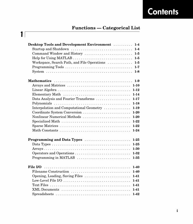
Contents
1Functions — Categorical List
Desktop Tools and Development Environment . . . . . . . . . . 1-4Startup and Shutdown . . . . . . . . . . . . . . . . . . . . . . . . . . . . . . . . 1-4Command Window and History . . . . . . . . . . . . . . . . . . . . . . . . . 1-5Help for Using MATLAB . . . . . . . . . . . . . . . . . . . . . . . . . . . . . . . 1-5Workspace, Search Path, and File Operations . . . . . . . . . . . . . 1-5Programming Tools . . . . . . . . . . . . . . . . . . . . . . . . . . . . . . . . . . . 1-7System . . . . . . . . . . . . . . . . . . . . . . . . . . . . . . . . . . . . . . . . . . . . . 1-8
Mathematics . . . . . . . . . . . . . . . . . . . . . . . . . . . . . . . . . . . . . . . . . 1-9Arrays and Matrices . . . . . . . . . . . . . . . . . . . . . . . . . . . . . . . . . 1-10Linear Algebra . . . . . . . . . . . . . . . . . . . . . . . . . . . . . . . . . . . . . . 1-12Elementary Math . . . . . . . . . . . . . . . . . . . . . . . . . . . . . . . . . . . 1-14Data Analysis and Fourier Transforms . . . . . . . . . . . . . . . . . . 1-17Polynomials . . . . . . . . . . . . . . . . . . . . . . . . . . . . . . . . . . . . . . . . 1-18Interpolation and Computational Geometry . . . . . . . . . . . . . . 1-19Coordinate System Conversion . . . . . . . . . . . . . . . . . . . . . . . . . 1-20Nonlinear Numerical Methods . . . . . . . . . . . . . . . . . . . . . . . . . 1-20Specialized Math . . . . . . . . . . . . . . . . . . . . . . . . . . . . . . . . . . . . 1-22Sparse Matrices . . . . . . . . . . . . . . . . . . . . . . . . . . . . . . . . . . . . . 1-22Math Constants . . . . . . . . . . . . . . . . . . . . . . . . . . . . . . . . . . . . . 1-24
Programming and Data Types . . . . . . . . . . . . . . . . . . . . . . . . 1-25Data Types . . . . . . . . . . . . . . . . . . . . . . . . . . . . . . . . . . . . . . . . . 1-25Arrays . . . . . . . . . . . . . . . . . . . . . . . . . . . . . . . . . . . . . . . . . . . . . 1-30Operators and Operations . . . . . . . . . . . . . . . . . . . . . . . . . . . . . 1-32Programming in MATLAB . . . . . . . . . . . . . . . . . . . . . . . . . . . . 1-35
File I/O . . . . . . . . . . . . . . . . . . . . . . . . . . . . . . . . . . . . . . . . . . . . . 1-40Filename Construction . . . . . . . . . . . . . . . . . . . . . . . . . . . . . . . 1-40Opening, Loading, Saving Files . . . . . . . . . . . . . . . . . . . . . . . . 1-41Low-Level File I/O . . . . . . . . . . . . . . . . . . . . . . . . . . . . . . . . . . . 1-41Text Files . . . . . . . . . . . . . . . . . . . . . . . . . . . . . . . . . . . . . . . . . . 1-41XML Documents . . . . . . . . . . . . . . . . . . . . . . . . . . . . . . . . . . . . 1-41Spreadsheets . . . . . . . . . . . . . . . . . . . . . . . . . . . . . . . . . . . . . . . 1-42

ii Contents
Scientific Data . . . . . . . . . . . . . . . . . . . . . . . . . . . . . . . . . . . . . . 1-42Audio and Audio/Video . . . . . . . . . . . . . . . . . . . . . . . . . . . . . . . 1-43Images . . . . . . . . . . . . . . . . . . . . . . . . . . . . . . . . . . . . . . . . . . . . . 1-43Internet Exchange . . . . . . . . . . . . . . . . . . . . . . . . . . . . . . . . . . . 1-44
Graphics . . . . . . . . . . . . . . . . . . . . . . . . . . . . . . . . . . . . . . . . . . . . 1-45Basic Plots and Graphs . . . . . . . . . . . . . . . . . . . . . . . . . . . . . . . 1-45Annotating Plots . . . . . . . . . . . . . . . . . . . . . . . . . . . . . . . . . . . . 1-46Specialized Plotting . . . . . . . . . . . . . . . . . . . . . . . . . . . . . . . . . . 1-46Bit-Mapped Images . . . . . . . . . . . . . . . . . . . . . . . . . . . . . . . . . . 1-49Printing . . . . . . . . . . . . . . . . . . . . . . . . . . . . . . . . . . . . . . . . . . . . 1-49Handle Graphics . . . . . . . . . . . . . . . . . . . . . . . . . . . . . . . . . . . . 1-49
3-D Visualization . . . . . . . . . . . . . . . . . . . . . . . . . . . . . . . . . . . . . 1-52Surface and Mesh Plots . . . . . . . . . . . . . . . . . . . . . . . . . . . . . . . 1-52View Control . . . . . . . . . . . . . . . . . . . . . . . . . . . . . . . . . . . . . . . . 1-53Lighting . . . . . . . . . . . . . . . . . . . . . . . . . . . . . . . . . . . . . . . . . . . 1-55Transparency . . . . . . . . . . . . . . . . . . . . . . . . . . . . . . . . . . . . . . . 1-55Volume Visualization . . . . . . . . . . . . . . . . . . . . . . . . . . . . . . . . . 1-55
Creating Graphical User Interfaces . . . . . . . . . . . . . . . . . . . . 1-56Predefined Dialog Boxes . . . . . . . . . . . . . . . . . . . . . . . . . . . . . . 1-56Deploying User Interfaces . . . . . . . . . . . . . . . . . . . . . . . . . . . . . 1-57Developing User Interfaces . . . . . . . . . . . . . . . . . . . . . . . . . . . . 1-57User Interface Objects . . . . . . . . . . . . . . . . . . . . . . . . . . . . . . . . 1-57Finding Objects from Callbacks . . . . . . . . . . . . . . . . . . . . . . . . 1-57
2Functions — Alphabetical List

1Functions — Categorical List
The MATLAB® Function Reference contains descriptions of all MATLAB commands and functions.
Select a category from the following table to see a list of related functions.
See Simulink®, Stateflow®, Real-Time Workshop®, and the individual toolboxes for lists of their functions
Desktop Tools and Development Environment
Startup, Command Window, help, editing and debugging, tuning, other general functions
Mathematics Arrays and matrices, linear algebra, data analysis, other areas of mathematics
Programming and Data Types
Function/expression evaluation, program control, function handles, object oriented programming, error handling, operators, data types, dates and times, timers
File I/O General and low-level file I/O, plus specific file formats, like audio, spreadsheet, HDF, images
Graphics Line plots, annotating graphs, specialized plots, images, printing, Handle Graphics®
3-D Visualization Surface and mesh plots, view control, lighting and transparency, volume visualization.
Creating Graphical User Interface
GUIDE, programming graphical user interfaces.
External Interfaces Java, COM, Serial Port functions.

1 Functions — Categorical List
1-4
Desktop Tools and Development EnvironmentGeneral functions for working in MATLAB, including functions for startup, Command Window, help, and editing and debugging.
Startup and Shutdownexit Terminate MATLAB (same as quit)finish MATLAB termination M-filegenpath Generate a path stringmatlab Start MATLAB (UNIX systems)matlab Start MATLAB (Windows systems)matlabrc MATLAB startup M-file for single user systems or administratorsprefdir Return directory containing preferences, history, and layout filespreferences Display Preferences dialog box for MATLAB and related productsquit Terminate MATLABstartup MATLAB startup M-file for user-defined options
“Startup and Shutdown” Startup and shutdown options
“Command Window and History”
Controlling Command Window and History
“Help for Using MATLAB”
Finding information
“Workspace, Search Path, and File Operations”
File, search path, variable management
“Programming Tools” Editing and debugging, source control, Notebook
“System” Identifying current computer, license, product version, and more

Desktop Tools and Development Environment
1-5
Command Window and Historyclc Clear Command WindowcommandhistoryOpen the Command History, or select it if already opencommandwindowOpen the Command Window, or select it if already opendiary Save session to filedos Execute DOS command and return resultformat Control display format for outputhome Move cursor to upper left corner of Command Windowmatlab: Run specified function via hyperlink (matlabcolon)more Control paged output for Command Windowperl Call Perl script using appropriate operating system executablesystem Execute operating system command and return resultunix Execute UNIX command and return result
Help for Using MATLABdoc Display online documentation in MATLAB Help browserdemo Access product demos via Help browserdocopt Web browser for UNIX platformsdocsearch Open Help browser Search pane and run search for specified termhelp Display help for MATLAB functions in Command Windowhelpbrowser Display Help browser for access to full online documentation and demoshelpwin Provide access to and display M-file help for all functionsinfo Display Release Notes for MathWorks productslookfor Search for specified keyword in all help entriesplayshow Run published M-file demosupport Open MathWorks Technical Support Web pageweb Open Web site or file in Web browser or Help browserwhatsnew Display Release Notes for MathWorks products
Workspace, Search Path, and File Operations• “Workspace”
• “Search Path”
• “File Operations”

1 Functions — Categorical List
1-6
Workspaceassignin Assign value to workspace variableclear Remove items from workspace, freeing up system memoryevalin Execute string containing MATLAB expression in a workspaceexist Check if variables or functions are definedopenvar Open workspace variable in Array Editor for graphical editingpack Consolidate workspace memoryuiimport Open Import Wizard, the graphical user interface to import datawhich Locate functions and fileswho, whos List variables in the workspaceworkspace Display Workspace browser, a tool for managing the workspace
Search Pathaddpath Add directories to MATLAB search pathgenpath Generate path stringpartialpath Partial pathnamepath View or change the MATLAB directory search pathpath2rc Replaced by savepathpathdef List of directories in the MATLAB search pathpathsep Return path separator for current platformpathtool Open Set Path dialog box to view and change MATLAB pathrestoredefaultpathRestore the default search pathrmpath Remove directories from MATLAB search pathsavepath Save current MATLAB search path to pathdef.m file
File Operationscd Change working directorycopyfile Copy file or directorydelete Delete files or graphics objectsdir Display directory listingexist Check if variables or functions are definedfileattrib Set or get attributes of file or directoryfilebrowser Display Current Directory browser, a tool for viewing fileslookfor Search for specified keyword in all help entriesls List directory on UNIXmatlabroot Return root directory of MATLAB installationmkdir Make new directorymovefile Move file or directorypwd Display current directoryrecycle Set option to move deleted files to recycle folderrehash Refresh function and file system path cachesrmdir Remove directory

Desktop Tools and Development Environment
1-7
type List fileweb Open Web site or file in Web browser or Help browserwhat List MATLAB specific files in current directorywhich Locate functions and files
See also “File I/O” functions.
Programming Tools• “Editing and Debugging”
• “Performance Improvement and Tuning Tools and Techniques”
• “Source Control”
• “Publishing”
Editing and Debuggingdbclear Clear breakpointsdbcont Resume executiondbdown Change local workspace contextdbquit Quit debug modedbstack Display function call stackdbstatus List all breakpointsdbstep Execute one or more lines from current breakpointdbstop Set breakpointsdbtype List M-file with line numbersdbup Change local workspace contextdebug M-file debugging functionsedit Edit or create M-filekeyboard Invoke the keyboard in an M-file
Performance Improvement and Tuning Tools and Techniquesmemory Help for memory limitationsmlint Check M-files for possible problems, and report resultsmlintrpt Run mlint for file or directory, reporting results in Web browserpack Consolidate workspace memoryprofile Profile the execution time for a functionprofsave Save profile report in HTML formatrehash Refresh function and file system path cachessparse Create sparse matrixzeros Create array of all zeros
1 Functions — Categorical List
1-8
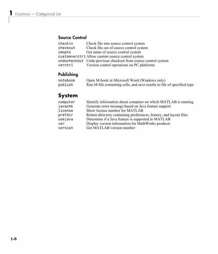
Source Controlcheckin Check file into source control systemcheckout Check file out of source control systemcmopts Get name of source control systemcustomverctrlAllow custom source control systemundocheckout Undo previous checkout from source control systemverctrl Version control operations on PC platforms
Publishingnotebook Open M-book in Microsoft Word (Windows only)publish Run M-file containing cells, and save results to file of specified type
Systemcomputer Identify information about computer on which MATLAB is runningjavachk Generate error message based on Java feature supportlicense Show license number for MATLABprefdir Return directory containing preferences, history, and layout filesusejava Determine if a Java feature is supported in MATLABver Display version information for MathWorks productsversion Get MATLAB version number

Mathematics
1-9
MathematicsFunctions for working with arrays and matrices, linear algebra, data analysis, and other areas of mathematics.
“Arrays and Matrices” Basic array operators and operations, creation of elementary and specialized arrays and matrices
“Linear Algebra” Matrix analysis, linear equations, eigenvalues, singular values, logarithms, exponentials, factorization
“Elementary Math” Trigonometry, exponentials and logarithms, complex values, rounding, remainders, discrete math
“Data Analysis and Fourier Transforms”
Descriptive statistics, finite differences, correlation, filtering and convolution, fourier transforms
“Polynomials” Multiplication, division, evaluation, roots, derivatives, integration, eigenvalue problem, curve fitting, partial fraction expansion
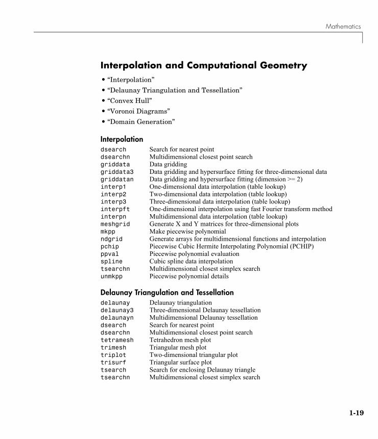
“Interpolation and Computational Geometry”
Interpolation, Delaunay triangulation and tessellation, convex hulls, Voronoi diagrams, domain generation
“Coordinate System Conversion”
Conversions between Cartesian and polar or spherical coordinates
“Nonlinear Numerical Methods”
Differential equations, optimization, integration
“Specialized Math” Airy, Bessel, Jacobi, Legendre, beta, elliptic, error, exponential integral, gamma functions
“Sparse Matrices” Elementary sparse matrices, operations, reordering algorithms, linear algebra, iterative methods, tree operations
“Math Constants” Pi, imaginary unit, infinity, Not-a-Number, largest and smallest positive floating point numbers, floating point relative accuracy

1 Functions — Categorical List
1-10
Arrays and Matrices• “Basic Information”
• “Operators”
• “Operations and Manipulation”
• “Elementary Matrices and Arrays”
• “Specialized Matrices”
Basic Informationdisp Display arraydisplay Display arrayisempty True for empty matrixisequal True if arrays are identicalisfloat True for floating-point arraysisinteger True for integer arraysislogical True for logical arrayisnumeric True for numeric arraysisscalar True for scalarsissparse True for sparse matrixisvector True for vectorslength Length of vectorndims Number of dimensionsnumel Number of elementssize Size of matrix
Operators+ Addition+ Unary plus- Subtraction- Unary minus* Matrix multiplication^ Matrix power\ Backslash or left matrix divide/ Slash or right matrix divide' Transpose.' Nonconjugated transpose.* Array multiplication (element-wise).^ Array power (element-wise).\ Left array divide (element-wise)./ Right array divide (element-wise)
Mathematics
1-11
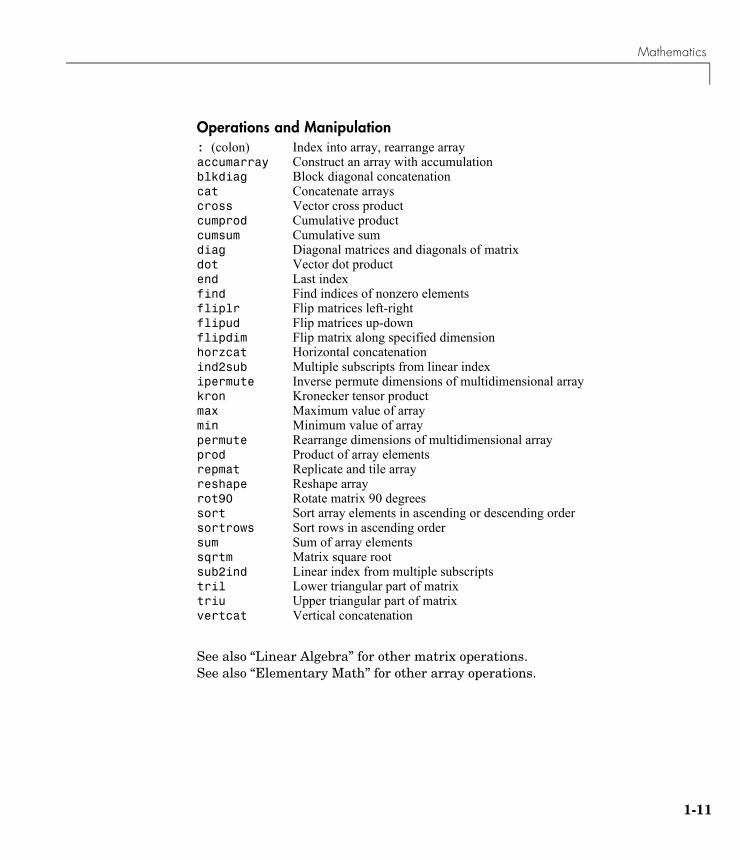
Operations and Manipulation: (colon) Index into array, rearrange arrayaccumarray Construct an array with accumulationblkdiag Block diagonal concatenationcat Concatenate arrayscross Vector cross productcumprod Cumulative productcumsum Cumulative sumdiag Diagonal matrices and diagonals of matrixdot Vector dot productend Last indexfind Find indices of nonzero elementsfliplr Flip matrices left-rightflipud Flip matrices up-downflipdim Flip matrix along specified dimensionhorzcat Horizontal concatenationind2sub Multiple subscripts from linear indexipermute Inverse permute dimensions of multidimensional arraykron Kronecker tensor productmax Maximum value of arraymin Minimum value of arraypermute Rearrange dimensions of multidimensional arrayprod Product of array elementsrepmat Replicate and tile arrayreshape Reshape arrayrot90 Rotate matrix 90 degreessort Sort array elements in ascending or descending ordersortrows Sort rows in ascending ordersum Sum of array elementssqrtm Matrix square rootsub2ind Linear index from multiple subscriptstril Lower triangular part of matrixtriu Upper triangular part of matrixvertcat Vertical concatenation
See also “Linear Algebra” for other matrix operations.See also “Elementary Math” for other array operations.

1 Functions — Categorical List
1-12
Elementary Matrices and Arrays: (colon) Regularly spaced vectorblkdiag Construct block diagonal matrix from input argumentsdiag Diagonal matrices and diagonals of matrixeye Identity matrixfreqspace Frequency spacing for frequency responselinspace Generate linearly spaced vectorslogspace Generate logarithmically spaced vectorsmeshgrid Generate X and Y matrices for three-dimensional plotsndgrid Arrays for multidimensional functions and interpolationones Create array of all onesrand Uniformly distributed random numbers and arraysrandn Normally distributed random numbers and arraysrepmat Replicate and tile arrayzeros Create array of all zeros
Specialized Matricescompan Companion matrixgallery Test matriceshadamard Hadamard matrixhankel Hankel matrixhilb Hilbert matrixinvhilb Inverse of Hilbert matrixmagic Magic squarepascal Pascal matrixrosser Classic symmetric eigenvalue test problemtoeplitz Toeplitz matrixvander Vandermonde matrixwilkinson Wilkinson’s eigenvalue test matrix
Linear Algebra• “Matrix Analysis”
• “Linear Equations”
• “Eigenvalues and Singular Values”
• “Matrix Logarithms and Exponentials”
• “Factorization”

Mathematics
1-13
Matrix Analysiscond Condition number with respect to inversioncondeig Condition number with respect to eigenvaluesdet Determinantnorm Matrix or vector normnormest Estimate matrix 2-normnull Null spaceorth Orthogonalizationrank Matrix rankrcond Matrix reciprocal condition number estimaterref Reduced row echelon formsubspace Angle between two subspacestrace Sum of diagonal elements
Linear Equations\ and / Linear equation solutionchol Cholesky factorizationcholinc Incomplete Cholesky factorizationcond Condition number with respect to inversioncondest 1-norm condition number estimatefunm Evaluate general matrix functioninv Matrix inverselinsolve Solve linear systems of equationslscov Least squares solution in presence of known covariancelsqnonneg Nonnegative least squareslu LU matrix factorizationluinc Incomplete LU factorizationpinv Moore-Penrose pseudoinverse of matrixqr Orthogonal-triangular decompositionrcond Matrix reciprocal condition number estimate
Eigenvalues and Singular Valuesbalance Improve accuracy of computed eigenvaluescdf2rdf Convert complex diagonal form to real block diagonal formcondeig Condition number with respect to eigenvalueseig Eigenvalues and eigenvectorseigs Eigenvalues and eigenvectors of sparse matrixgsvd Generalized singular value decompositionhess Hessenberg form of matrixpoly Polynomial with specified rootspolyeig Polynomial eigenvalue problemqz QZ factorization for generalized eigenvalues

1 Functions — Categorical List
1-14
rsf2csf Convert real Schur form to complex Schur formschur Schur decompositionsvd Singular value decompositionsvds Singular values and vectors of sparse matrix
Matrix Logarithms and Exponentialsexpm Matrix exponentiallogm Matrix logarithmsqrtm Matrix square root
Factorizationbalance Diagonal scaling to improve eigenvalue accuracycdf2rdf Complex diagonal form to real block diagonal formchol Cholesky factorizationcholinc Incomplete Cholesky factorizationcholupdate Rank 1 update to Cholesky factorizationlu LU matrix factorizationluinc Incomplete LU factorizationplanerot Givens plane rotationqr Orthogonal-triangular decompositionqrdelete Delete column or row from QR factorizationqrinsert Insert column or row into QR factorizationqrupdate Rank 1 update to QR factorizationqz QZ factorization for generalized eigenvaluesrsf2csf Real block diagonal form to complex diagonal form
Elementary Math• “Trigonometric”
• “Exponential”
• “Complex”
• “Rounding and Remainder”
• “Discrete Math (e.g., Prime Factors)”
Mathematics
1-15
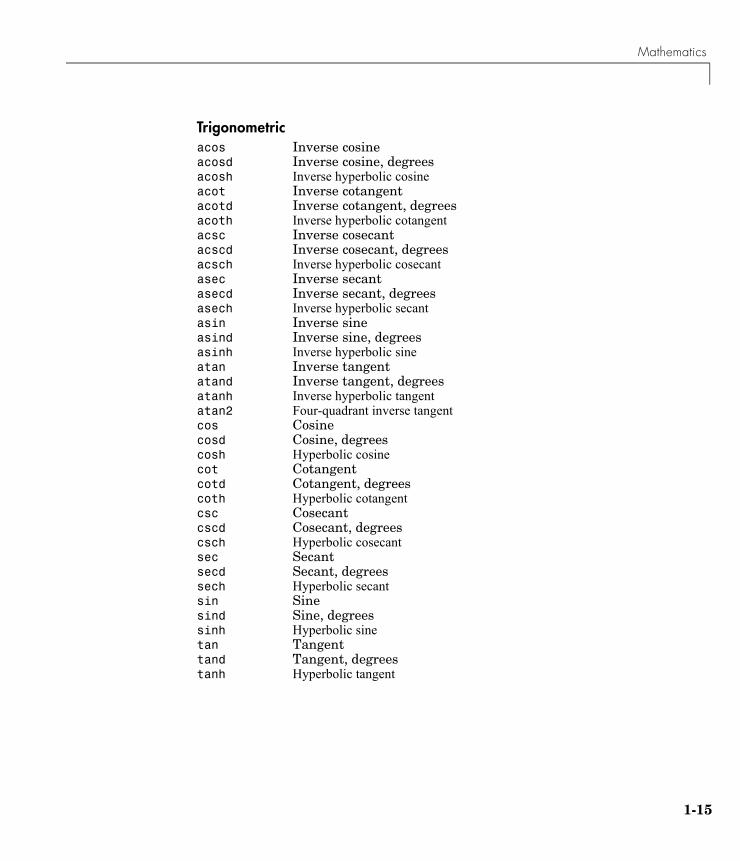
Trigonometricacos Inverse cosineacosd Inverse cosine, degreesacosh Inverse hyperbolic cosineacot Inverse cotangentacotd Inverse cotangent, degreesacoth Inverse hyperbolic cotangentacsc Inverse cosecantacscd Inverse cosecant, degreesacsch Inverse hyperbolic cosecantasec Inverse secantasecd Inverse secant, degreesasech Inverse hyperbolic secantasin Inverse sineasind Inverse sine, degreesasinh Inverse hyperbolic sineatan Inverse tangentatand Inverse tangent, degreesatanh Inverse hyperbolic tangentatan2 Four-quadrant inverse tangentcos Cosinecosd Cosine, degreescosh Hyperbolic cosinecot Cotangentcotd Cotangent, degreescoth Hyperbolic cotangentcsc Cosecantcscd Cosecant, degreescsch Hyperbolic cosecantsec Secantsecd Secant, degreessech Hyperbolic secantsin Sinesind Sine, degreessinh Hyperbolic sinetan Tangenttand Tangent, degreestanh Hyperbolic tangent
1 Functions — Categorical List
1-16
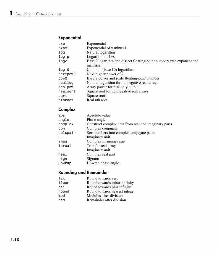
Exponentialexp Exponentialexpm1 Exponential of x minus 1log Natural logarithmlog1p Logarithm of 1+xlog2 Base 2 logarithm and dissect floating-point numbers into exponent and
mantissalog10 Common (base 10) logarithmnextpow2 Next higher power of 2pow2 Base 2 power and scale floating-point numberreallog Natural logarithm for nonnegative real arraysrealpow Array power for real-only outputrealsqrt Square root for nonnegative real arrayssqrt Square rootnthroot Real nth root
Complexabs Absolute valueangle Phase anglecomplex Construct complex data from real and imaginary partsconj Complex conjugatecplxpair Sort numbers into complex conjugate pairsi Imaginary unitimag Complex imaginary partisreal True for real arrayj Imaginary unitreal Complex real partsign Signumunwrap Unwrap phase angle
Rounding and Remainderfix Round towards zerofloor Round towards minus infinityceil Round towards plus infinityround Round towards nearest integermod Modulus after divisionrem Remainder after division

Mathematics
1-17
Discrete Math (e.g., Prime Factors)factor Prime factorsfactorial Factorial functiongcd Greatest common divisorisprime True for prime numberslcm Least common multiplenchoosek All combinations of N elements taken K at a timeperms All possible permutationsprimes Generate list of prime numbersrat, rats Rational fraction approximation
Data Analysis and Fourier Transforms• “Basic Operations”
• “Finite Differences”
• “Correlation”
• “Filtering and Convolution”
• “Fourier Transforms”
Basic Operationscumprod Cumulative productcumsum Cumulative sumcumtrapz Cumulative trapezoidal numerical integrationmax Maximum elements of arraymean Average or mean value of arraysmedian Median value of arraysmin Minimum elements of arrayprod Product of array elementssort Sort array elements in ascending or descending ordersortrows Sort rows in ascending orderstd Standard deviationsum Sum of array elementstrapz Trapezoidal numerical integrationvar Variance
Finite Differencesdel2 Discrete Laplaciandiff Differences and approximate derivativesgradient Numerical gradient

1 Functions — Categorical List
1-18
Correlationcorrcoef Correlation coefficientscov Covariance matrixsubspace Angle between two subspaces
Filtering and Convolutionconv Convolution and polynomial multiplicationconv2 Two-dimensional convolutionconvn N-dimensional convolutiondeconv Deconvolution and polynomial divisiondetrend Linear trend removalfilter Filter data with infinite impulse response (IIR) or finite impulse response
(FIR) filterfilter2 Two-dimensional digital filtering
Fourier Transformsabs Absolute value and complex magnitudeangle Phase anglefft One-dimensional discrete Fourier transformfft2 Two-dimensional discrete Fourier transformfftn N-dimensional discrete Fourier Transformfftshift Shift DC component of discrete Fourier transform to center of spectrumfftw Interface to the FFTW library run-time algorithm for tuning FFTs ifft Inverse one-dimensional discrete Fourier transformifft2 Inverse two-dimensional discrete Fourier transformifftn Inverse multidimensional discrete Fourier transformifftshift Inverse fast Fourier transform shiftnextpow2 Next power of twounwrap Correct phase angles
Polynomialsconv Convolution and polynomial multiplicationdeconv Deconvolution and polynomial divisionpoly Polynomial with specified rootspolyder Polynomial derivativepolyeig Polynomial eigenvalue problempolyfit Polynomial curve fittingpolyint Analytic polynomial integrationpolyval Polynomial evaluationpolyvalm Matrix polynomial evaluationresidue Convert between partial fraction expansion and polynomial coefficientsroots Polynomial roots
Mathematics
1-19
Interpolation and Computational Geometry• “Interpolation”
• “Delaunay Triangulation and Tessellation”
• “Convex Hull”
• “Voronoi Diagrams”
• “Domain Generation”
Interpolationdsearch Search for nearest pointdsearchn Multidimensional closest point searchgriddata Data griddinggriddata3 Data gridding and hypersurface fitting for three-dimensional datagriddatan Data gridding and hypersurface fitting (dimension >= 2)interp1 One-dimensional data interpolation (table lookup)interp2 Two-dimensional data interpolation (table lookup)interp3 Three-dimensional data interpolation (table lookup)interpft One-dimensional interpolation using fast Fourier transform methodinterpn Multidimensional data interpolation (table lookup)meshgrid Generate X and Y matrices for three-dimensional plotsmkpp Make piecewise polynomialndgrid Generate arrays for multidimensional functions and interpolationpchip Piecewise Cubic Hermite Interpolating Polynomial (PCHIP)ppval Piecewise polynomial evaluationspline Cubic spline data interpolationtsearchn Multidimensional closest simplex searchunmkpp Piecewise polynomial details
Delaunay Triangulation and Tessellationdelaunay Delaunay triangulationdelaunay3 Three-dimensional Delaunay tessellationdelaunayn Multidimensional Delaunay tessellationdsearch Search for nearest pointdsearchn Multidimensional closest point searchtetramesh Tetrahedron mesh plottrimesh Triangular mesh plottriplot Two-dimensional triangular plottrisurf Triangular surface plottsearch Search for enclosing Delaunay triangletsearchn Multidimensional closest simplex search

1 Functions — Categorical List
1-20
Convex Hullconvhull Convex hullconvhulln Multidimensional convex hullpatch Create patch graphics objectplot Linear two-dimensional plottrisurf Triangular surface plot
Voronoi Diagramsdsearch Search for nearest pointpatch Create patch graphics objectplot Linear two-dimensional plotvoronoi Voronoi diagramvoronoin Multidimensional Voronoi diagrams
Domain Generationmeshgrid Generate X and Y matrices for three-dimensional plotsndgrid Generate arrays for multidimensional functions and interpolation
Coordinate System Conversion
Cartesiancart2sph Transform Cartesian to spherical coordinatescart2pol Transform Cartesian to polar coordinatespol2cart Transform polar to Cartesian coordinatessph2cart Transform spherical to Cartesian coordinates
Nonlinear Numerical Methods• “Ordinary Differential Equations (IVP)”
• “Delay Differential Equations”
• “Boundary Value Problems”
• “Partial Differential Equations”
• “Optimization”
• “Numerical Integration (Quadrature)”

Mathematics
1-21
Ordinary Differential Equations (IVP)ode113 Solve non-stiff differential equations, variable order methodode15i Solve fully implicit differential equations, variable order methodode15s Solve stiff ODEs and DAEs Index 1, variable order methodode23 Solve non-stiff differential equations, low order methodode23s Solve stiff differential equations, low order methodode23t Solve moderately stiff ODEs and DAEs Index 1, trapezoidal ruleode23tb Solve stiff differential equations, low order methodode45 Solve non-stiff differential equations, medium order methododextend Extend the solution of an initial value problemodeget Get ODE options parametersodeset Create/alter ODE options structuredecic Compute consistent initial conditions for ode15ideval Evaluate solution of differential equation problem
Delay Differential Equationsdde23 Solve delay differential equations with constant delaysddeget Get DDE options parametersddeset Create/alter DDE options structuredeval Evaluate solution of differential equation problem
Boundary Value Problemsbvp4c Solve boundary value problems for ODEsbvpget Get BVP options parametersbvpset Create/alter BVP options structuredeval Evaluate solution of differential equation problem
Partial Differential Equationspdepe Solve initial-boundary value problems for parabolic-elliptic PDEspdeval Evaluates by interpolation solution computed by pdepe
Optimizationfminbnd Scalar bounded nonlinear function minimizationfminsearch Multidimensional unconstrained nonlinear minimization, by
Nelder-Mead direct search methodfzero Scalar nonlinear zero findinglsqnonneg Linear least squares with nonnegativity constraintsoptimset Create or alter optimization options structureoptimget Get optimization parameters from options structure

1 Functions — Categorical List
1-22
Numerical Integration (Quadrature)quad Numerically evaluate integral, adaptive Simpson quadrature (low order)quadl Numerically evaluate integral, adaptive Lobatto quadrature (high order)quadv Vectorized quadraturedblquad Numerically evaluate double integraltriplequad Numerically evaluate triple integral
Specialized Mathairy Airy functionsbesselh Bessel functions of third kind (Hankel functions)besseli Modified Bessel function of first kindbesselj Bessel function of first kindbesselk Modified Bessel function of second kindbessely Bessel function of second kindbeta Beta functionbetainc Incomplete beta functionbetaln Logarithm of beta functionellipj Jacobi elliptic functionsellipke Complete elliptic integrals of first and second kinderf Error functionerfc Complementary error functionerfcinv Inverse complementary error functionerfcx Scaled complementary error functionerfinv Inverse error functionexpint Exponential integralgamma Gamma functiongammainc Incomplete gamma functiongammaln Logarithm of gamma functionlegendre Associated Legendre functionspsi Psi (polygamma) function
Sparse Matrices • “Elementary Sparse Matrices”
• “Full to Sparse Conversion”
• “Working with Sparse Matrices”
• “Reordering Algorithms”
• “Linear Algebra”
• “Linear Equations (Iterative Methods)”
• “Tree Operations”

Mathematics
1-23
Elementary Sparse Matricesspdiags Sparse matrix formed from diagonalsspeye Sparse identity matrixsprand Sparse uniformly distributed random matrixsprandn Sparse normally distributed random matrixsprandsym Sparse random symmetric matrix
Full to Sparse Conversionfind Find indices of nonzero elementsfull Convert sparse matrix to full matrixsparse Create sparse matrixspconvert Import from sparse matrix external format
Working with Sparse Matricesissparse True for sparse matrixnnz Number of nonzero matrix elementsnonzeros Nonzero matrix elementsnzmax Amount of storage allocated for nonzero matrix elementsspalloc Allocate space for sparse matrixspfun Apply function to nonzero matrix elementsspones Replace nonzero sparse matrix elements with onesspparms Set parameters for sparse matrix routinesspy Visualize sparsity pattern
Reordering Algorithmscolamd Column approximate minimum degree permutationcolmmd Column minimum degree permutationcolperm Column permutationdmperm Dulmage-Mendelsohn permutationrandperm Random permutationsymamd Symmetric approximate minimum degree permutationsymmmd Symmetric minimum degree permutationsymrcm Symmetric reverse Cuthill-McKee permutation
Linear Algebracholinc Incomplete Cholesky factorizationcondest 1-norm condition number estimateeigs Eigenvalues and eigenvectors of sparse matrixluinc Incomplete LU factorizationnormest Estimate matrix 2-normsprank Structural ranksvds Singular values and vectors of sparse matrix

1 Functions — Categorical List
1-24
Linear Equations (Iterative Methods)bicg BiConjugate Gradients methodbicgstab BiConjugate Gradients Stabilized methodcgs Conjugate Gradients Squared methodgmres Generalized Minimum Residual methodlsqr LSQR implementation of Conjugate Gradients on Normal Equationsminres Minimum Residual methodpcg Preconditioned Conjugate Gradients methodqmr Quasi-Minimal Residual methodspaugment Form least squares augmented systemsymmlq Symmetric LQ method
Tree Operationsetree Elimination treeetreeplot Plot elimination treegplot Plot graph, as in “graph theory”symbfact Symbolic factorization analysistreelayout Lay out tree or foresttreeplot Plot picture of tree
Math Constantseps Floating-point relative accuracyi Imaginary unitInf Infinity, ∞ intmax Largest possible value of specified integer typeintmin Smallest possible value of specified integer typej Imaginary unitNaN Not-a-Numberpi Ratio of a circle’s circumference to its diameter, π realmax Largest positive floating-point numberrealmin Smallest positive floating-point number

Programming and Data Types
1-25
Programming and Data Types
Functions to store and operate on data at either the MATLAB command line or in programs and scripts. Functions to write, manage, and execute MATLAB programs.
Data Types• “Numeric”
• “Characters and Strings”
• “Structures”
• “Cell Arrays”
• “Data Type Conversion”
• “Determine Data Type”
“Data Types” Numeric, character, structures, cell arrays, and data type conversion
“Arrays” Basic array operations and manipulation
“Operators and Operations” Special characters and arithmetic, bit-wise, relational, logical, set, date and time operations
“Programming in MATLAB” M-files, function/expression evaluation, program control, function handles, object oriented programming, error handling

1 Functions — Categorical List
1-26
Numeric[ ] Array constructorcat Concatenate arraysclass Return object’s class name (e.g., numeric)find Find indices and values of nonzero array elementsintmax Largest possible value of specified integer typeintmin Smallest possible value of specified integer typeintwarning Enable or disable integer warningsipermute Inverse permute dimensions of multidimensional arrayisa Determine if item is object of given class (e.g., numeric)isequal Determine if arrays are numerically equalisequalwithequalnansTest for equality, treating NaNs as equalisnumeric Determine if item is numeric arrayisreal Determine if all array elements are real numbersisscalar True for scalars (1-by-1 matrices)isvector True for vectors (1-by-N or N-by-1 matrices)permute Rearrange dimensions of multidimensional arrayrealmax Largest positive floating-point numberrealmin Smallest positive floating-point numberreshape Reshape arraysqueeze Remove singleton dimensions from arrayzeros Create array of all zeros
Characters and Strings
Description of Strings in MATLAB
strings Describes MATLAB string handling
Creating and Manipulating Strings
blanks Create string of blankschar Create character array (string)cellstr Create cell array of strings from character arraydatestr Convert to date string formatdeblank Strip trailing blanks from the end of stringlower Convert string to lower casesprintf Write formatted data to stringsscanf Read string under format controlstrcat String concatenation
Programming and Data Types
1-27
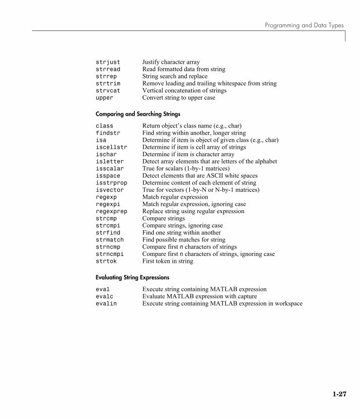
strjust Justify character arraystrread Read formatted data from stringstrrep String search and replacestrtrim Remove leading and trailing whitespace from stringstrvcat Vertical concatenation of stringsupper Convert string to upper case
Comparing and Searching Strings
class Return object’s class name (e.g., char)findstr Find string within another, longer stringisa Determine if item is object of given class (e.g., char)iscellstr Determine if item is cell array of stringsischar Determine if item is character arrayisletter Detect array elements that are letters of the alphabetisscalar True for scalars (1-by-1 matrices)isspace Detect elements that are ASCII white spacesisstrprop Determine content of each element of stringisvector True for vectors (1-by-N or N-by-1 matrices)regexp Match regular expressionregexpi Match regular expression, ignoring caseregexprep Replace string using regular expressionstrcmp Compare stringsstrcmpi Compare strings, ignoring casestrfind Find one string within anotherstrmatch Find possible matches for stringstrncmp Compare first n characters of stringsstrncmpi Compare first n characters of strings, ignoring casestrtok First token in string
Evaluating String Expressions
eval Execute string containing MATLAB expressionevalc Evaluate MATLAB expression with captureevalin Execute string containing MATLAB expression in workspace

1 Functions — Categorical List
1-28
Structurescell2struct Cell array to structure array conversionclass Return object’s class name (e.g., struct)deal Deal inputs to outputsfieldnames Field names of structureisa Determine if item is object of given class (e.g., struct)isequal Determine if arrays are numerically equalisfield Determine if item is structure array fieldisscalar True for scalars (1-by-1 matrices)isstruct Determine if item is structure arrayisvector True for vectors (1-by-N or N-by-1 matrices)orderfields Order fields of a structure arrayrmfield Remove structure fieldsstruct Create structure arraystruct2cell Structure to cell array conversion
Cell Arrays Construct cell arraycell Construct cell arraycellfun Apply function to each element in cell arraycellstr Create cell array of strings from character arraycell2mat Convert cell array of matrices into single matrixcell2struct Cell array to structure array conversioncelldisp Display cell array contentscellplot Graphically display structure of cell arraysclass Return object’s class name (e.g., cell)deal Deal inputs to outputsisa Determine if item is object of given class (e.g., cell)iscell Determine if item is cell arrayiscellstr Determine if item is cell array of stringsisequal Determine if arrays are numerically equalisscalar True for scalars (1-by-1 matrices)isvector True for vectors (1-by-N or N-by-1 matrices)mat2cell Divide matrix up into cell array of matricesnum2cell Convert numeric array into cell arraystruct2cell Structure to cell array conversion

Programming and Data Types
1-29
Data Type Conversion
Numeric
double Convert to double-precisionint8 Convert to signed 8-bit integerint16 Convert to signed 16-bit integerint32 Convert to signed 32-bit integerint64 Convert to signed 64-bit integersingle Convert to single-precisionuint8 Convert to unsigned 8-bit integeruint16 Convert to unsigned 16-bit integeruint32 Convert to unsigned 32-bit integeruint64 Convert to unsigned 64-bit integer
String to Numeric
base2dec Convert base N number string to decimal numberbin2dec Convert binary number string to decimal numberhex2dec Convert hexadecimal number string to decimal numberhex2num Convert hexadecimal number string to double numberstr2double Convert string to double-precision numberstr2num Convert string to number
Numeric to String
char Convert to character array (string)dec2base Convert decimal to base N number in stringdec2bin Convert decimal to binary number in stringdec2hex Convert decimal to hexadecimal number in stringint2str Convert integer to stringmat2str Convert a matrix to stringnum2str Convert number to string
Other Conversions
cell2mat Convert cell array of matrices into single matrixcell2struct Convert cell array to structure arraydatestr Convert serial date number to stringfunc2str Convert function handle to function name stringlogical Convert numeric to logical arraymat2cell Divide matrix up into cell array of matricesnum2cell Convert a numeric array to cell arraystr2func Convert function name string to function handlestruct2cell Convert structure to cell array

1 Functions — Categorical List
1-30
Determine Data Typeis* Detect stateisa Determine if item is object of given classiscell Determine if item is cell arrayiscellstr Determine if item is cell array of stringsischar Determine if item is character arrayisfield Determine if item is character arrayisfloat True for floating-point arraysisinteger True for integer arraysisjava Determine if item is Java objectislogical Determine if item is logical arrayisnumeric Determine if item is numeric arrayisobject Determine if item is MATLAB OOPs objectisreal Determine if all array elements are real numbersisstruct Determine if item is MATLAB structure array
Arrays• “Array Operations”
• “Basic Array Information”
• “Array Manipulation”
• “Elementary Arrays”
Array Operations[ ] Array constructor, Array row element separator; Array column element separator: Specify range of array elementsend Indicate last index of array+ Addition or unary plus- Subtraction or unary minus.* Array multiplication./ Array right division.\ Array left division.^ Array power.' Array (nonconjugated) transpose

Programming and Data Types
1-31
Basic Array Informationdisp Display text or arraydisplay Overloaded method to display text or arrayisempty Determine if array is emptyisequal Determine if arrays are numerically equalisequalwithequalnansTest for equality, treating NaNs as equalislogical Determine if item is logical arrayisnumeric Determine if item is numeric arrayisscalar Determine if item is a scalarisvector Determine if item is a vectorlength Length of vectorndims Number of array dimensionsnumel Number of elements in matrix or cell arraysize Array dimensions
Array Manipulation: Specify range of array elementsblkdiag Construct block diagonal matrix from input argumentscat Concatenate arrayscircshift Shift array circularlyfind Find indices and values of nonzero elementsfliplr Flip matrices left-rightflipud Flip matrices up-downflipdim Flip array along specified dimensionhorzcat Horizontal concatenationind2sub Subscripts from linear indexipermute Inverse permute dimensions of multidimensional arraypermute Rearrange dimensions of multidimensional arrayrepmat Replicate and tile arrayreshape Reshape arrayrot90 Rotate matrix 90 degreesshiftdim Shift dimensionssort Sort array elements in ascending or descending ordersortrows Sort rows in ascending ordersqueeze Remove singleton dimensionssub2ind Single index from subscriptsvertcat Horizontal concatenation

1 Functions — Categorical List
1-32
Elementary Arrays: Regularly spaced vectorblkdiag Construct block diagonal matrix from input argumentseye Identity matrixlinspace Generate linearly spaced vectorslogspace Generate logarithmically spaced vectorsmeshgrid Generate X and Y matrices for three-dimensional plotsndgrid Generate arrays for multidimensional functions and interpolationones Create array of all onesrand Uniformly distributed random numbers and arraysrandn Normally distributed random numbers and arrayszeros Create array of all zeros
Operators and Operations• “Special Characters”
• “Arithmetic Operations”
• “Bit-wise Operations”
• “Relational Operations”
• “Logical Operations”
• “Set Operations”
• “Date and Time Operations”
Special Characters: Specify range of array elements ( ) Pass function arguments, or prioritize operations[ ] Construct array Construct cell array. Decimal point, or structure field separator... Continue statement to next line, Array row element separator; Array column element separator% Insert comment line into code! Command to operating system= Assignment

Programming and Data Types
1-33
Arithmetic Operations+ Plus- Minus. Decimal point= Assignment* Matrix multiplication/ Matrix right division\ Matrix left division^ Matrix power' Matrix transpose.* Array multiplication (element-wise)./ Array right division (element-wise).\ Array left division (element-wise).^ Array power (element-wise).' Array transpose
Bit-wise Operationsbitand Bit-wise ANDbitcmp Bit-wise complementbitor Bit-wise ORbitmax Maximum floating-point integerbitset Set bit at specified positionbitshift Bit-wise shiftbitget Get bit at specified positionbitxor Bit-wise XOR
Relational Operations< Less than<= Less than or equal to> Greater than>= Greater than or equal to== Equal to~= Not equal to

1 Functions — Categorical List
1-34
Logical Operations&& Logical AND|| Logical OR& Logical AND for arrays| Logical OR for arrays~ Logical NOTall Test to determine if all elements are nonzeroany Test for any nonzero elementsfalse False arrayfind Find indices and values of nonzero elementsis* Detect stateisa Determine if item is object of given classiskeyword Determine if string is MATLAB keywordisvarname Determine if string is valid variable namelogical Convert numeric values to logicaltrue True arrayxor Logical EXCLUSIVE OR
Set Operationsintersect Set intersection of two vectorsismember Detect members of setsetdiff Return set difference of two vectorsissorted Determine if set elements are in sorted ordersetxor Set exclusive or of two vectorsunion Set union of two vectorsunique Unique elements of vector
Date and Time Operationsaddtodate Modify particular field of date numbercalendar Calendar for specified monthclock Current time as date vectorcputime Elapsed CPU timedate Current date stringdatenum Serial date numberdatestr Convert serial date number to stringdatevec Date componentseomday End of monthetime Elapsed timenow Current date and timetic, toc Stopwatch timerweekday Day of the week

Programming and Data Types
1-35
Programming in MATLAB
• “M-File Functions and Scripts”
• “Evaluation of Expressions and Functions”
• “Timer Functions”
• “Variables and Functions in Memory”
• “Control Flow”
• “Function Handles”
• “Object-Oriented Programming”
• “Error Handling”
• “MEX Programming”
M-File Functions and Scripts( ) Pass function arguments% Insert comment line into code... Continue statement to next linedepfun List dependent functions of M-file or P-filedepdir List dependent directories of M-file or P-fileecho Echo M-files during executionfunction Function M-filesinput Request user inputinputname Input argument namemfilename Name of currently running M-filenamelengthmaxReturn maximum identifier lengthnargin Number of function input argumentsnargout Number of function output argumentsnargchk Check number of input argumentsnargoutchk Validate number of output argumentspcode Create preparsed pseudocode file (P-file)script Describes script M-filevarargin Accept variable number of argumentsvarargout Return variable number of arguments

1 Functions — Categorical List
1-36
Evaluation of Expressions and Functionsbuiltin Execute built-in function from overloaded methodcellfun Apply function to each element in cell arrayecho Echo M-files during executioneval Interpret strings containing MATLAB expressionsevalc Evaluate MATLAB expression with captureevalin Evaluate expression in workspacefeval Evaluate functioniskeyword Determine if item is MATLAB keywordisvarname Determine if item is valid variable namepause Halt execution temporarilyrun Run script that is not on current pathscript Describes script M-filesymvar Determine symbolic variables in expressiontic, toc Stopwatch timer
Timer Functionsdelete Delete timer object from memorydisp Display information about timer objectget Retrieve information about timer object propertiesisvalid Determine if timer object is valid set Display or set timer object propertiesstart Start a timerstartat Start a timer at a specific timerstop Stop a timertimer Create a timer objecttimerfind Return an array of all visible timer objects in memorytimerfindall Return an array of all timer objects in memorywait Block command line until timer completes
Variables and Functions in Memoryassignin Assign value to workspace variablegenvarname Construct valid variable name from stringglobal Define global variablesinmem Return names of functions in memoryisglobal Determine if item is global variablemislocked True if M-file cannot be clearedmlock Prevent clearing M-file from memorymunlock Allow clearing M-file from memorynamelengthmaxReturn maximum identifier lengthpack Consolidate workspace memorypersistent Define persistent variablerehash Refresh function and file system caches

Programming and Data Types
1-37
Control Flowbreak Terminate execution of for loop or while loopcase Case switchcatch Begin catch blockcontinue Pass control to next iteration of for or while loopelse Conditionally execute statementselseif Conditionally execute statementsend Terminate conditional statements, or indicate last indexerror Display error messagesfor Repeat statements specific number of timesif Conditionally execute statementsotherwise Default part of switch statementreturn Return to invoking functionswitch Switch among several cases based on expressiontry Begin try blockwhile Repeat statements indefinite number of times
Function Handlesclass Return object’s class name (e.g. function_handle)feval Evaluate functionfunction_handle
Describes function handle data typefunctions Return information about function handlefunc2str Constructs function name string from function handleisa Determine if item is object of given class (e.g. function_handle)isequal Determine if function handles are equalstr2func Constructs function handle from function name string
Object-Oriented Programming
MATLAB Classes and Objects
class Create object or return class of objectfieldnames List public fields belonging to object,inferiorto Establish inferior class relationshipisa Determine if item is object of given classisobject Determine if item is MATLAB OOPs objectloadobj User-defined extension of load function for user objectsmethods Display information on class methodsmethodsview Display information on class methods in separate windowsaveobj User-defined extension of save function for user objectssubsasgn Overloaded method for A(I)=B, AI=B, and A.field=B

1 Functions — Categorical List
1-38
subsindex Overloaded method for X(A)subsref Overloaded method for A(I), AI and A.fieldsubstruct Create structure argument for subsasgn or subsrefsuperiorto Establish superior class relationship
Java Classes and Objects
cell Convert Java array object to cell arrayclass Return class name of Java objectclear Clear Java import list or Java class definitionsdepfun List Java classes used by M-fileexist Determine if item is Java classfieldnames List public fields belonging to objectim2java Convert image to instance of Java image objectimport Add package or class to current Java import listinmem List names of Java classes loaded into memoryisa Determine if item is object of given classisjava Determine if item is Java objectjavaaddpath Add entries to dynamic Java class pathjavaArray Construct Java arrayjavachk Generate error message based on Java feature supportjavaclasspathSet and get dynamic Java class pathjavaMethod Invoke Java methodjavaObject Construct Java objectjavarmpath Remove entries from dynamic Java class pathmethods Display information on class methodsmethodsview Display information on class methods in separate windowusejava Determine if a Java feature is supported in MATLABwhich Display package and class name for method
Error Handlingcatch Begin catch block of try/catch statementerror Display error messageferror Query MATLAB about errors in file input or outputintwarning Enable or disable integer warningslasterr Return last error message generated by MATLABlasterror Last error message and related informationlastwarn Return last warning message issued by MATLABrethrow Reissue errortry Begin try block of try/catch statementwarning Display warning message

Programming and Data Types
1-39
MEX Programmingdbmex Enable MEX-file debugginginmem Return names of currently loaded MEX-filesmex Compile MEX-function from C or Fortran source codemexext Return MEX-filename extension

1 Functions — Categorical List
1-40
File I/OFunctions to read and write data to files of different format types.
To see a listing of file formats that are readable from MATLAB, go to file formats.
Filename Constructionfileparts Return parts of filenamefilesep Return directory separator for this platformfullfile Build full filename from partstempdir Return name of system's temporary directorytempname Return unique string for use as temporary filename
“Filename Construction” Get path, directory, filename information; construct filenames
“Opening, Loading, Saving Files” Open files; transfer data between files and MATLAB workspace
“Low-Level File I/O” Low-level operations that use a file identifier (e.g., fopen, fseek, fread)
“Text Files” Delimited or formatted I/O to text files
“XML Documents” Documents written in Extensible Markup Language
“Spreadsheets” Excel and Lotus 123 files
“Scientific Data” CDF, FITS, HDF formats
“Audio and Audio/Video” General audio functions; SparcStation, WAVE, AVI files
“Images” Graphics files
“Internet Exchange” URL, zip, and e-mail

File I/O
1-41
Opening, Loading, Saving Filesimportdata Load data from various types of filesload Load all or specific data from MAT or ASCII fileopen Open files of various types using appropriate editor or programsave Save all or specific data to MAT or ASCII fileuiimport Open Import Wizard, the graphical user interface to import datawinopen Open file in appropriate application (Windows only)
Low-Level File I/Ofclose Close one or more open filesfeof Test for end-of-fileferror Query MATLAB about errors in file input or outputfgetl Return next line of file as string without line terminator(s)fgets Return next line of file as string with line terminator(s)fopen Open file or obtain information about open filesfprintf Write formatted data to filefread Read binary data from filefrewind Rewind open filefscanf Read formatted data from filefseek Set file position indicatorftell Get file position indicatorfwrite Write binary data to file
Text Filescsvread Read numeric data from text file, using comma delimitercsvwrite Write numeric data to text file, using comma delimiterdlmread Read numeric data from text file, specifying your own delimiterdlmwrite Write numeric data to text file, specifying your own delimitertextread Read data from text file, write to multiple outputstextscan Read data from text file, convert and write to cell array
XML Documentsxmlread Parse XML documentxmlwrite Serialize XML Document Object Model nodexslt Transform XML document using XSLT engine

1 Functions — Categorical List
1-42
Spreadsheets
Microsoft Excel Functionsxlsfinfo Determine if file contains Microsoft Excel (.xls) spreadsheetxlsread Read Microsoft Excel spreadsheet file (.xls)xlswrite Write Microsoft Excel spreadsheet file (.xls)
Lotus123 Functionswk1read Read Lotus123 WK1 spreadsheet file into matrixwk1write Write matrix to Lotus123 WK1 spreadsheet file
Scientific Data
Common Data Format (CDF)cdfepoch Convert MATLAB date number or date string into CDF epochcdfinfo Return information about CDF filecdfread Read CDF filecdfwrite Write CDF file
Flexible Image Transport Systemfitsinfo Return information about FITS filefitsread Read FITS file
Hierarchical Data Format (HDF)hdf Interface to HDF4 fileshdfinfo Return information about HDF4 or HDF-EOS filehdfread Read HDF4 filehdftool Start HDF4 Import Toolhdf5 Describes HDF5 data type objectshdf5info Return information about HDF5 filehdf5read Read HDF5 filehdf5write Write data to file in HDF5 format
Band-Interleaved DatamultibandreadRead band-interleaved data from filemultibandwriteWrite band-interleaved data to file

File I/O
1-43
Audio and Audio/Video
Generalaudioplayer Create audio player objectaudiorecorderPerform real-time audio capturebeep Produce beep soundlin2mu Convert linear audio signal to mu-lawmmfileinfo Information about a multimedia filemu2lin Convert mu-law audio signal to linearsound Convert vector into soundsoundsc Scale data and play as sound
SPARCstation-Specific Sound Functionsauread Read NeXT/SUN (.au) sound fileauwrite Write NeXT/SUN (.au) sound file
Microsoft WAVE Sound Functionswavplay Play sound on PC-based audio output devicewavread Read Microsoft WAVE (.wav) sound filewavrecord Record sound using PC-based audio input devicewavwrite Write Microsoft WAVE (.wav) sound file
Audio/Video Interleaved (AVI) Functionsaddframe Add frame to AVI fileavifile Create new AVI fileaviinfo Return information about AVI fileaviread Read AVI fileclose Close AVI filemovie2avi Create AVI movie from MATLAB movie
Imagesim2java Convert image to instance of Java image objectimfinfo Return information about graphics fileimread Read image from graphics fileimwrite Write image to graphics file

1 Functions — Categorical List
1-44
Internet Exchangeftp Connect to FTP server, creating an FTP objectsendmail Send e-mail message (attachments optional) to list of addressesunzip Extract contents of zip fileurlread Read contents at URLurlwrite Save contents of URL to filezip Create compressed version of files in zip format

Graphics
1-45
Graphics2-D graphs, specialized plots (e.g., pie charts, histograms, and contour plots), function plotters, and Handle Graphics functions.
Basic Plots and Graphsbox Axis box for 2-D and 3-D plotserrorbar Plot graph with error barshold Hold current graphLineSpec Line specification syntaxloglog Plot using log-log scalespolar Polar coordinate plotplot Plot vectors or matrices. plot3 Plot lines and points in 3-D spaceplotyy Plot graphs with Y tick labels on the left and rightsemilogx Semi-log scale plotsemilogy Semi-log scale plotsubplot Create axes in tiled positions
Plotting ToolsfigurepaletteDisplay figure palette on figurepan Turn panning on or off.plotbrowser Display plot browser on figureplottools Start plotting toolspropertyeditorDisplay property editor on figurezoom Turn zooming on or off
Basic Plots and Graphs Linear line plots, log and semilog plots
Annotating Plots Titles, axes labels, legends, mathematical symbols
Specialized Plotting Bar graphs, histograms, pie charts, contour plots, function plotters
Bit-Mapped Images Display image object, read and write graphics file, convert to movie frames
Printing Printing and exporting figures to standard formats
Handle Graphics Creating graphics objects, setting properties, finding handles

1 Functions — Categorical List
1-46
Annotating Plots
annotation Create annotation objectsclabel Add contour labels to contour plotdatetick Date formatted tick labelsgtext Place text on 2-D graph using mouselegend Graph legend for lines and patchestexlabel Produce the TeX format from character stringtitle Titles for 2-D and 3-D plotsxlabel X-axis labels for 2-D and 3-D plotsylabel Y-axis labels for 2-D and 3-D plotszlabel Z-axis labels for 3-D plots
Annotation Object Properties
arrow Properties for annotation arrowsdoublearrow Properties for double-headed annotation arrowsellipse Properties for annotation ellipsesline Properties for annotation linesrectangle Properties for annotation rectanglestextarrow Properties for annotation textbox
Specialized Plotting• “Area, Bar, and Pie Plots”
• “Contour Plots”
• “Direction and Velocity Plots”
• “Discrete Data Plots”
• “Function Plots”
• “Histograms”
• “Polygons and Surfaces”
• “Scatter/Bubble Plots”
• “Animation”

Graphics
1-47
Area, Bar, and Pie Plotsarea Area plotbar Vertical bar chartbarh Horizontal bar chartbar3 Vertical 3-D bar chartbar3h Horizontal 3-D bar chartpareto Pareto charpie Pie plotpie3 3-D pie plot
Contour Plotscontour Contour (level curves) plotcontour3 3-D contour plotcontourc Contour computationcontourf Filled contour plotezcontour Easy to use contour plotterezcontourf Easy to use filled contour plotter
Direction and Velocity Plotscomet Comet plotcomet3 3-D comet plotcompass Compass plotfeather Feather plotquiver Quiver (or velocity) plotquiver3 3-D quiver (or velocity) plot
Discrete Data Plotsstem Plot discrete sequence datastem3 Plot discrete surface datastairs Stairstep graph
Function Plotsezcontour Easy to use contour plotterezcontourf Easy to use filled contour plotterezmesh Easy to use 3-D mesh plotterezmeshc Easy to use combination mesh/contour plotterezplot Easy to use function plotterezplot3 Easy to use 3-D parametric curve plotterezpolar Easy to use polar coordinate plotterezsurf Easy to use 3-D colored surface plotterezsurfc Easy to use combination surface/contour plotterfplot Plot a function

1 Functions — Categorical List
1-48
Histogramshist Plot histogramshistc Histogram countrose Plot rose or angle histogram
Polygons and Surfacesconvhull Convex hullcylinder Generate cylinderdelaunay Delaunay triangulationdsearch Search Delaunay triangulation for nearest pointellipsoid Generate ellipsoidfill Draw filled 2-D polygonsfill3 Draw filled 3-D polygons in 3-spaceinpolygon True for points inside a polygonal regionpcolor Pseudocolor (checkerboard) plotpolyarea Area of polygonribbon Ribbon plotslice Volumetric slice plotsphere Generate spheretsearch Search for enclosing Delaunay trianglevoronoi Voronoi diagramwaterfall Waterfall plot
Scatter/Bubble Plotsplotmatrix Scatter plot matrixscatter Scatter plotscatter3 3-D scatter plot
Animationframe2im Convert movie frame to indexed imagegetframe Capture movie frameim2frame Convert image to movie framemovie Play recorded movie framesnoanimate Change EraseMode of all objects to normal

Graphics
1-49
Bit-Mapped Imagesframe2im Convert movie frame to indexed imageimage Display image objectimagesc Scale data and display image objectimfinfo Information about graphics fileimformats Manage file format registryim2frame Convert image to movie frameim2java Convert image to instance of Java image objectimread Read image from graphics fileimwrite Write image to graphics fileind2rgb Convert indexed image to RGB image
Printingframeedit Edit print frame for Simulink and Stateflow diagramorient Hardcopy paper orientationpagesetupdlg Page setup dialog boxprint Print graph or save graph to fileprintdlg Print dialog boxprintopt Configure local printer defaultsprintpreview Preview figure to be printedsaveas Save figure to graphic file
Handle Graphics• Finding and Identifying Graphics Objects
• Object Creation Functions
• Figure Windows
• Axes Operations

1 Functions — Categorical List
1-50
Finding and Identifying Graphics Objectsallchild Find all children of specified objectsancestor Find ancestor of graphics objectcopyobj Make copy of graphics object and its childrendelete Delete files or graphics objectsfindall Find all graphics objects (including hidden handles)figflag Test if figure is on screenfindfigs Display off-screen visible figure windowsfindobj Find objects with specified property valuesgca Get current Axes handlegcbo Return object whose callback is currently executinggcbf Return handle of figure containing callback objectgco Return handle of current objectget Get object propertiesishandle True if value is valid object handleset Set object properties
Object Creation Functionsaxes Create axes objectfigure Create figure (graph) windowshggroup Create a group objecthgtransform Create a group to transformimage Create image (2-D matrix)light Create light object (illuminates Patch and Surface)line Create line object (3-D polylines)patch Create patch object (polygons)rectangle Create rectangle object (2-D rectangle)rootobject List of root propertiessurface Create surface (quadrilaterals)text Create text object (character strings)uicontextmenuCreate context menu (popup associated with object)
Plot Objectsareaseries Property listbarseries Property listcontourgroup Property listerrorbarseriesProperty listlineseries Property listquivergroup Property listscattergroup Property liststairseries Property liststemseries Property listsurfaceplot Property list
Graphics
1-51
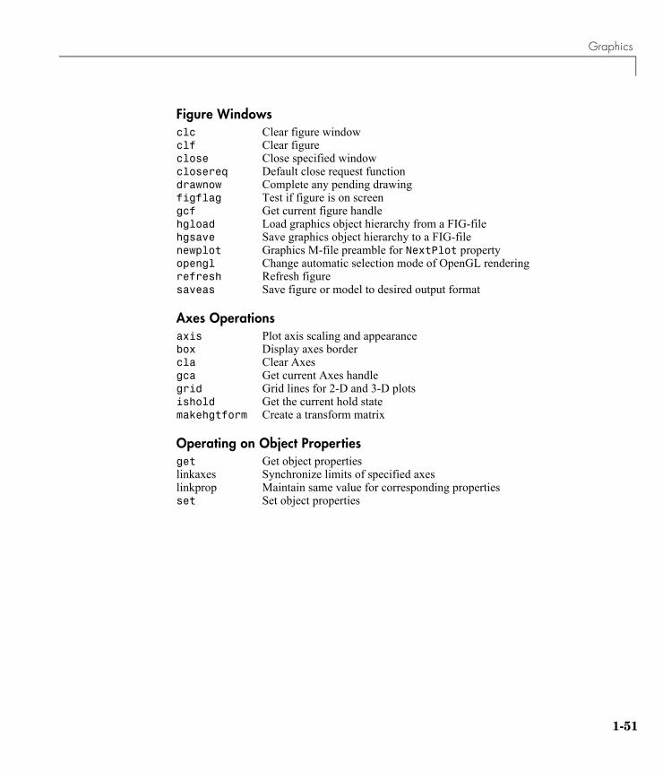
Figure Windowsclc Clear figure windowclf Clear figureclose Close specified windowclosereq Default close request functiondrawnow Complete any pending drawingfigflag Test if figure is on screengcf Get current figure handlehgload Load graphics object hierarchy from a FIG-filehgsave Save graphics object hierarchy to a FIG-filenewplot Graphics M-file preamble for NextPlot propertyopengl Change automatic selection mode of OpenGL renderingrefresh Refresh figuresaveas Save figure or model to desired output format
Axes Operationsaxis Plot axis scaling and appearancebox Display axes bordercla Clear Axesgca Get current Axes handlegrid Grid lines for 2-D and 3-D plotsishold Get the current hold statemakehgtform Create a transform matrix
Operating on Object Propertiesget Get object propertieslinkaxes Synchronize limits of specified axeslinkprop Maintain same value for corresponding propertiesset Set object properties

1 Functions — Categorical List
1-52
3-D VisualizationCreate and manipulate graphics that display 2-D matrix and 3-D volume data, controlling the view, lighting and transparency.
Surface and Mesh Plots• Creating Surfaces and Meshes
• Domain Generation
• Color Operations
• Colormaps
Creating Surfaces and Mesheshidden Mesh hidden line removal modemeshc Combination mesh/contourplotmesh 3-D mesh with reference planepeaks A sample function of two variablessurf 3-D shaded surface graphsurface Create surface low-level objectssurfc Combination surf/contourplotsurfl 3-D shaded surface with lightingtetramesh Tetrahedron mesh plottrimesh Triangular mesh plottriplot 2-D triangular plottrisurf Triangular surface plot
Domain Generationgriddata Data gridding and surface fittingmeshgrid Generation of X and Y arrays for 3-D plots
Surface and Mesh Plots Plot matrices, visualize functions of two variables, specify colormap
View Control Control the camera viewpoint, zooming, rotation, aspect ratio, set axis limits
Lighting Add and control scene lighting
Transparency Specify and control object transparency
Volume Visualization Visualize gridded volume data

3-D Visualization
1-53
Color Operationsbrighten Brighten or darken colormapcaxis Pseudocolor axis scalingcolormapeditorStart colormap editorcolorbar Display color bar (color scale)colordef Set up color defaultscolormap Set the color look-up table (list of colormaps)ColorSpec Ways to specify colorgraymon Graphics figure defaults set for grayscale monitorhsv2rgb Hue-saturation-value to red-green-blue conversionrgb2hsv RGB to HSVconversionrgbplot Plot colormapshading Color shading modespinmap Spin the colormapsurfnorm 3-D surface normalswhitebg Change axes background color for plots
Colormapsautumn Shades of red and yellow colormapbone Gray-scale with a tinge of blue colormapcontrast Gray colormap to enhance image contrastcool Shades of cyan and magenta colormapcopper Linear copper-tone colormapflag Alternating red, white, blue, and black colormapgray Linear gray-scale colormaphot Black-red-yellow-white colormaphsv Hue-saturation-value (HSV) colormapjet Variant of HSVlines Line color colormapprism Colormap of prism colorsspring Shades of magenta and yellow colormapsummer Shades of green and yellow colormapwinter Shades of blue and green colormap
View Control• Controlling the Camera Viewpoint
• Setting the Aspect Ratio and Axis Limits
• Object Manipulation
• Selecting Region of Interest

1 Functions — Categorical List
1-54
Controlling the Camera Viewpointcamdolly Move camera position and targetcamlookat View specific objectscamorbit Orbit about camera targetcampan Rotate camera target about camera positioncampos Set or get camera positioncamproj Set or get projection typecamroll Rotate camera about viewing axiscamtarget Set or get camera targetcameratoolbarControl camera toolbar programmaticallycamup Set or get camera up-vectorcamva Set or get camera view anglecamzoom Zoom camera in or outview 3-D graph viewpoint specification. viewmtx Generate view transformation matricesmakehgtform Create a transform matrix
Setting the Aspect Ratio and Axis Limitsdaspect Set or get data aspect ratiopbaspect Set or get plot box aspect ratioxlim Set or get the current x-axis limitsylim Set or get the current y-axis limitszlim Set or get the current z-axis limits
Object Manipulationpan Turns panning on or offreset Reset axis or figurerotate Rotate objects about specified origin and directionrotate3d Interactively rotate the view of a 3-D plotselectmoveresizeInteractively select, move, or resize objectszoom Zoom in and out on a 2-D plot
Selecting Region of Interestdragrect Drag XOR rectangles with mouserbbox Rubberband box

3-D Visualization
1-55
Lightingcamlight Cerate or position Lightlight Light object creation functionlightangle Position light in sphereical coordinateslighting Lighting modematerial Material reflectance mode
Transparencyalpha Set or query transparency properties for objects in current axesalphamap Specify the figure alphamapalim Set or query the axes alpha limits
Volume Visualizationconeplot Plot velocity vectors as cones in 3-D vector fieldcontourslice Draw contours in volume slice planecurl Compute curl and angular velocity of vector fielddivergence Compute divergence of vector fieldflow Generate scalar volume datainterpstreamspeedInterpolate streamline vertices from vector-field magnitudesisocaps Compute isosurface end-cap geometryisocolors Compute colors of isosurface verticesisonormals Compute normals of isosurface verticesisosurface Extract isosurface data from volume datareducepatch Reduce number of patch facesreducevolume Reduce number of elements in volume data setshrinkfaces Reduce size of patch facesslice Draw slice planes in volumesmooth3 Smooth 3-D datastream2 Compute 2-D stream line datastream3 Compute 3-D stream line datastreamline Draw stream lines from 2- or 3-D vector datastreamparticlesDraws stream particles from vector volume datastreamribbon Draws stream ribbons from vector volume datastreamslice Draws well-spaced stream lines from vector volume datastreamtube Draws stream tubes from vector volume datasurf2patch Convert surface data to patch datasubvolume Extract subset of volume data setvolumebounds Return coordinate and color limits for volume (scalar and vector)

1 Functions — Categorical List
1-56
Creating Graphical User InterfacesPredefined dialog boxes and functions to control GUI programs.
Predefined Dialog Boxesdialog Create dialog boxerrordlg Create error dialog boxhelpdlg Display help dialog boxinputdlg Create input dialog boxlistdlg Create list selection dialog boxmsgbox Create message dialog boxpagesetupdlg Page setup dialog boxprintdlg Display print dialog boxquestdlg Create question dialog boxuigetdir Display dialog box to retrieve name of directoryuigetfile Display dialog box to retrieve name of file for readinguiputfile Display dialog box to retrieve name of file for writinguisetcolor Set ColorSpec using dialog boxuisetfont Set font using dialog boxwaitbar Display wait barwarndlg Create warning dialog box
Predefined Dialog Boxes Dialog boxes for error, user input, waiting, etc.
Deploying User Interfaces
Launching GUIs, creating the handles structure
Developing User Interfaces
Starting GUIDE, managing application data, getting user input
User Interface Objects Creating GUI components
Finding Objects from Callbacks
Finding object handles from within callbacks functions
GUI Utility Functions Moving objects, text wrapping
Controlling Program Execution
Wait and resume based on user input

Creating Graphical User Interfaces
1-57
Deploying User Interfacesguidata Store or retrieve application dataguihandles Create a structure of handles movegui Move GUI figure onscreenopenfig Open or raise GUI figure
Developing User Interfacesguide Open GUI Layout Editorinspect Display Property Inspector
Working with Application Datagetappdata Get value of application dataisappdata True if application data existsrmappdata Remove application datasetappdata Specify application data
Interactive User Inputginput Graphical input from a mouse or cursorwaitfor Wait for conditions before resuming executionwaitforbuttonpressWait for key/buttonpress over figure
User Interface Objectsmenu Generate menu of choices for user inputuibuttongroupCreate component to exclusively manage radiobuttons and togglebuttonsuicontextmenuCreate context menuuicontrol Create user interface controluimenu Create user interface menuuipanel Create panel container objectuipushtool Create toolbar push buttonuitoggletool Create toolbar toggle buttonuitoolbar Create toolbar
Finding Objects from Callbacksfindall Find all graphics objectsfindfigs Display off-screen visible figure windowsfindobj Find specific graphics objectgcbf Return handle of figure containing callback objectgcbo Return handle of object whose callback is executing

1 Functions — Categorical List
1-58

2Functions — Alphabetical List

pack
2-1596
2packPurpose Consolidate workspace memory
Syntax packpack filenamepack('filename')
Description pack frees up needed space by reorganizing information so it only uses the minimum memory required. You must run pack from a directory for which you have write permission. Running pack clears all variables not in the base workspace, so persistent variables, for example, will be cleared.
pack filename accepts an optional filename for the temporary file used to hold the variables. Otherwise, it uses the file named pack.tmp. You must run pack from a directory for which you have write permission.
pack('filename') is the function form of pack.
Remarks The pack function does not affect the amount of memory allocated to the MATLAB process. You must quit MATLAB to free up this memory.
Since MATLAB uses a heap method of memory management, extended MATLAB sessions may cause memory to become fragmented. When memory is fragmented, there may be plenty of free space, but not enough contiguous memory to store a new large variable.
If you get the Out of memory message from MATLAB, the pack function may find you some free memory without forcing you to delete variables.
The pack function frees space by:
• Saving all variables in the base workspace to disk in a temporary file called pack.tmp
• Clearing all variables and functions from memory
• Reloading the base workspace variables back from pack.tmp
• Deleting the temporary file pack.tmp

pack
2-1597
If you use pack and there is still not enough free memory to proceed, you must clear some variables. If you run out of memory often, you can allocate larger matrices earlier in the MATLAB session and use these system-specific tips:
• UNIX: Ask your system manager to increase your swap space.
• Windows: Increase virtual memory using the Windows Control Panel.
To maintain persistent variables when you run pack, use mlock in the function.
Examples Change the current directory to one that is writable, run pack, and return to the previous directory.
cwd = pwd;cd(tempdir);packcd(cwd)
See Also clear, memory

pagesetupdlg
2-1598
2pagesetupdlgPurpose Page position dialog box
Syntax dlg = pagesetupdlg(fig)
Description dlg = pagesetupdlg(fig) creates a dialog box from which a set of pagelayout properties for the figure window, fig, can be set.
pagesetupdlg implements the "Page Setup..." option in the Figure File Menu.
Unlike pagedlg, pagesetupdlg currently only supports setting the layout for a single figure. fig must be a single figure handle, not a vector of figures or a simulink diagram.
See Also printpreview, printopt

pan
2-1599
2panPurpose Pan the view of a graph interactively
Syntax pan onpan xonpan yonpan offpanpan(figure_handle,...)
Description pan on truns on mouse-based panning in the current figure.
pan xon turns on panning only in the x direction in the current figure.
pan yon turns on panning only in the y direction in the current figure.
pan off turns panning off in the current figure.
pan toggles the pan state in the current figure on or off.
pan(figure_handle,...) sets the pan state in the specified figure.
See Also zoom, linkaxes
“Object Manipulation” for related functions

pareto
2-1600
2paretoPurpose Pareto chart
Syntax pareto(Y)pareto(Y,names)pareto(Y,X)H = pareto(...)
Description Pareto charts display the values in the vector Y as bars drawn in descending order.
pareto(Y) labels each bar with its element index in Y.
pareto(Y,names) labels each bar with the associated name in the string matrix or cell array names.
pareto(Y,X) labels each bar with the associated value from X.
H = pareto(...) returns a combination of patch and line object handles.
See Also hist, bar

partialpath
2-1601
2partialpathPurpose Partial pathname
Description A partial pathname is a pathname relative to the MATLAB path, matlabpath. It is used to locate private and method files, which are usually hidden, or to restrict the search for files when more than one file with the given name exists.
A partial pathname contains the last component, or last several components, of the full pathname separated by /. For example, matfun/trace, private/children, and demos/clown.mat are valid partial pathnames. Specifying the @ in method directory names is optional.
Partial pathnames make it easy to find toolbox or MATLAB relative files on your path, independent of the location where MATLAB is installed.
Many commands accept partial pathnames instead of a full pathname. Some of these commands are
help, type, load, exist, what, which, edit, dbtype, dbstop, dbclear, and fopen
Examples The following example uses a partial pathname:
what graph2d/@figobj
M-files in directory matlabroot\toolbox\matlab\graph2d\@figobj
deselectall doresize figobj middrag subsasgndoclick enddrag get set subsref
P-files in directory matlabroot\toolbox\matlab\graph2d\@figobj
deselectall doresize figobj middrag subsasgndoclick enddrag get set subsref
The @ in the class directory name @figobj is not necessary. You get the same response from the following command:
what graph2d/figobj
See Also fileparts, matlabroot, path

pascal
2-1602
2pascalPurpose Pascal matrix
Syntax A = pascal(n)A = pascal(n,1)A = pascal(n,2)
Description A = pascal(n) returns the Pascal matrix of order n: a symmetric positive definite matrix with integer entries taken from Pascal’s triangle. The inverse of A has integer entries.
A = pascal(n,1) returns the lower triangular Cholesky factor (up to the signs of the columns) of the Pascal matrix. It is involutary, that is, it is its own inverse.
A = pascal(n,2) returns a transposed and permuted version of pascal(n,1). A is a cube root of the identity matrix.
Examples pascal(4) returns
1 1 1 11 2 3 41 3 6 101 4 10 20
A = pascal(3,2) produces
A = 1 1 1 -2 -1 0 1 0 0
See Also chol

patch
2-1603
2patchPurpose Create patch graphics object
Syntax patch(X,Y,C)patch(X,Y,Z,C)patch(FV)patch(...'PropertyName',PropertyValue...)patch('PropertyName',PropertyValue...) PN/PV pairs onlyhandle = patch(...)
Description patch is the low-level graphics function for creating patch graphics objects. A patch object is one or more polygons defined by the coordinates of its vertices. You can specify the coloring and lighting of the patch. See Creating 3-D Models with Patches for more information on using patch objects.
patch(X,Y,C) adds the filled two-dimensional patch to the current axes. The elements of X and Y specify the vertices of a polygon. If X and Y are matrices, MATLAB draws one polygon per column. C determines the color of the patch. It can be a single ColorSpec, one color per face, or one color per vertex (see “Remarks”). If C is a 1-by-3 vector, it is assumed to be an RGB triplet, specifying a color directly.
patch(X,Y,Z,C) creates a patch in three-dimensional coordinates.
patch(FV) creates a patch using structure FV, which contains the fields vertices, faces, and optionally facevertexdata. These fields correspond to the Vertices, Faces, and FaceVertexCData patch properties.
patch(...'PropertyName',PropertyValue...) follows the X, Y, (Z), and C arguments with property name/property value pairs to specify additional patch properties.
patch('PropertyName',PropertyValue,...) specifies all properties using property name/property value pairs. This form enables you to omit the color specification because MATLAB uses the default face color and edge color unless you explicitly assign a value to the FaceColor and EdgeColor properties. This form also allows you to specify the patch using the Faces and Vertices properties instead of x-, y-, and z-coordinates. See the “Examples” section for more information.
patch
2-1604
handle = patch(...) returns the handle of the patch object it creates.
Remarks Unlike high-level area creation functions, such as fill or area, patch does not check the settings of the figure and axes NextPlot properties. It simply adds the patch object to the current axes.
If the coordinate data does not define closed polygons, patch closes the polygons. The data can define concave or intersecting polygons. However, if the edges of an individual patch face intersect themselves, the resulting face may or may not be completely filled. In that case, it is better to break up the face into smaller polygons.
Specifying Patch PropertiesYou can specify properties as property name/property value pairs, structure arrays, and cell arrays (see the set and get reference pages for examples of how to specify these data types).
There are two patch properties that specify color:
• CData — Use when specifying x-, y-, and z-coordinates (XData, YData, ZData).
• FaceVertexCData — Use when specifying vertices and connection matrix (Vertices and Faces).
The CData and FaceVertexCData properties accept color data as indexed or true color (RGB) values. See the CData and FaceVertexCData property descriptions for information on how to specify color.
Indexed color data can represent either direct indices into the colormap or scaled values that map the data linearly to the entire colormap (see the caxis function for more information on this scaling). The CDataMapping property determines how MATLAB interprets indexed color data.

patch
2-1605
Color Data InterpretationYou can specify patch colors as
• A single color for all faces
• One color for each face, enabling flat coloring
• One color for each vertex, enabling interpolated coloring
The following tables summarize how MATLAB interprets color data defined by the CData and FaceVertexCData properties.
Interpretation of the CData Property
Color Specification
FaceVertexCData
CData
Indexed
True Color
direct
scaled
(CDataMapping)
Color Interpretation by MATLAB
Color Mapping
[X,Y,Z]Data CData Required for Results ObtainedDimensions Indexed True Color
m-by-n scalar 1-by-1-by-3 Use the single color specified for all patch faces. Edges can be only a single color.

patch
2-1606
Interpretation of the FaceVertexCData Property
Examples This example creates a patch object using two different methods:
• Specifying x-, y-, and z-coordinates and color data (XData, YData, ZData, and CData properties)
• Specifying vertices, the connection matrix, and color data (Vertices, Faces, FaceVertexCData, and FaceColor properties)
m-by-n 1-by-n(n >= 4)
1-by-n-by-3 Use one color for each patch face. Edges can be only a single color.
m-by-n m-by-n m-by-n-3 Assign a color to each vertex. Patch faces can be flat (a single color) or interpolated. Edges can be flat or interpolated.
[X,Y,Z]Data CData Required for Results ObtainedDimensions Indexed True Color
Vertices Faces FaceVertexCData Required for
Results Obtained
Dimensions Dimensions Indexed True Color
m-by-n k-by-3 scalar 1-by-3 Use the single color specified for all patch faces. Edges can be only a single color.
m-by-n k-by-3 k-by-1 k-by-3 Use one color for each patch face. Edges can be only a single color.
m-by-n k-by-3 m-by-1 m-by-3 Assign a color to each vertex. Patch faces can be flat (a single color) or interpolated. Edges can be flat or interpolated.

patch
2-1607
Specifying X, Y, and Z CoordinatesThe first approach specifies the coordinates of each vertex. In this example, the coordinate data defines two triangular faces, each having three vertices. Using true color, the top face is set to white and the bottom face to gray.
x = [0 0;0 1;1 1];y = [1 1;2 2;2 1];z = [1 1;1 1;1 1];tcolor(1,1,1:3) = [1 1 1];tcolor(1,2,1:3) = [.7 .7 .7];patch(x,y,z,tcolor)
Notice that each face shares two vertices with the other face (V1-V4 and V3-V5).
Specifying Vertices and FacesThe Vertices property contains the coordinates of each unique vertex defining the patch. The Faces property specifies how to connect these vertices to form each face of the patch. For this example, two vertices share the same location so you need to specify only four of the six vertices. Each row contains the x-, y-, and z-coordinates of each vertex.
vert = [0 1 1;0 2 1;1 2 1;1 1 1];
There are only two faces, defined by connecting the vertices in the order indicated.
0 0.2 0.4 0.6 0.8 11
1.1
1.2
1.3
1.4
1.5
1.6
1.7
1.8
1.9
2
V2 V3V5
V6V1
V4
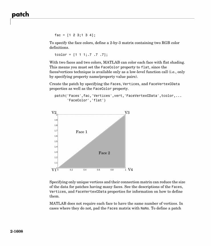
patch
2-1608
fac = [1 2 3;1 3 4];
To specify the face colors, define a 2-by-3 matrix containing two RGB color definitions.
tcolor = [1 1 1;.7 .7 .7];
With two faces and two colors, MATLAB can color each face with flat shading. This means you must set the FaceColor property to flat, since the faces/vertices technique is available only as a low-level function call (i.e., only by specifying property name/property value pairs).
Create the patch by specifying the Faces, Vertices, and FaceVertexCData properties as well as the FaceColor property.
patch('Faces',fac,'Vertices',vert,'FaceVertexCData',tcolor,...'FaceColor','flat')
Specifying only unique vertices and their connection matrix can reduce the size of the data for patches having many faces. See the descriptions of the Faces, Vertices, and FaceVertexCData properties for information on how to define them.
MATLAB does not require each face to have the same number of vertices. In cases where they do not, pad the Faces matrix with NaNs. To define a patch
0 0.2 0.4 0.6 0.8 11
1.1
1.2
1.3
1.4
1.5
1.6
1.7
1.8
1.9
2
V1
V2 V3
V4
Face 1
Face 2

patch
2-1609
with faces that do not close, add one or more NaNs to the row in the Vertices matrix that defines the vertex you do not want connected.
Object Hierarchy
Setting Default PropertiesYou can set default patch properties on the axes, figure, and root levels:
set(0,'DefaultPatchPropertyName',PropertyValue...)set(gcf,'DefaultPatchPropertyName',PropertyValue...)set(gca,'DefaultPatchPropertyName',PropertyValue...)
PropertyName is the name of the patch property and PropertyValue is the value you are specifying. Use set and get to access patch properties.
Property List The following table lists all patch properties and provides a brief description of each. The property name links take you to an expanded description of the properties.
Patch
Axes
Patch
Group Object
Property Name Property Description Property Value
Data Defining the Object
Faces Connection matrix for Vertices Values: m-by-n matrixDefault: [1,2,3]
Vertices Matrix of x-, y-, and z-coordinates of the vertices (used with Faces)
Value: matrixDefault: [0,1;1,1;0,0]
XData The x-coordinates of the vertices of the patch
Value: vector or matrixDefault: [0;1;0]

patch
2-1610
YData The y-coordinates of the vertices of the patch
Value: vector or matrixDefault: [1;1;0]
ZData The z-coordinates of the vertices of the patch
Value: vector or matrixDefault: [] (empty matrix)
Specifying Color
CData Color data for use with the XData/YData/ZData method
Value: scalar, vector, or matrixDefault: [] (empty matrix)
CDataMapping Controls mapping of CData to colormap
Values: scaled, directDefault: scaled
EdgeColor Color of face edges Values: ColorSpec, none, flat, interpDefault: ColorSpec
FaceColor Color of face Values: ColorSpec, none, flat, interpDefault: ColorSpec
FaceVertexCData Color data for use with Faces/Vertices method
Value: matrixDefault: [] (empty matrix)
MarkerEdgeColor Color of marker or the edge color for filled markers
Values: ColorSpec, none, autoDefault: auto
MarkerFaceColor Fill color for markers that are closed shapes
Values: ColorSpec, none, autoDefault: none
Controlling the Effects of Lights
AmbientStrength Intensity of the ambient light Value: scalar >=0 and <=1Default: 0.3
Property Name Property Description Property Value

patch
2-1611
BackFaceLighting Controls lighting of faces pointing away from camera
Values: unlit, lit, reverselitDefault: reverselit
DiffuseStrength Intensity of diffuse light Value: scalar >=0 and <=1Default: 0.6
EdgeLighting Method used to light edges Values: none, flat, gouraud, phongDefault: none
FaceLighting Method used to light edges Values: none, flat, gouraud, phongDefault: none
NormalMode MATLAB generated or user-specified normal vectors
Values: auto, manualDefault: auto
SpecularColorReflectance Composite color of specularly reflected light
Value: scalar 0 to 1Default: 1
SpecularExponent Harshness of specular reflection Value: scalar >= 1Default: 10
SpecularStrength Intensity of specular light Value: scalar >=0 and <=1Default: 0.9
VertexNormals Vertex normal vectors Value: matrix
Defining Edges and Markers
LineStyle Select from five line styles. Values: −, −−, :, −., noneDefault: −
LineWidth The width of the edge in points Value: scalarDefault: 0.5 points
Marker Marker symbol to plot at data points
Values: see Marker propertyDefault: none
Property Name Property Description Property Value

patch
2-1612
MarkerSize Size of marker in points Value: size in pointsDefault: 6
Specifying Transparency
AlphaDataMapping Transparency mapping method Values: none, direct, scaledDefault: scaled
EdgeAlpha Transparency of the edges of patch faces
Values: scalar, flat, interpDefault: 1 (opaque)
FaceAlpha Transparency of the patch face Values: scalar, flat, interpDefault: 1 (opaque)
FaceVertexAlphaData Face and vertex transparency data
Value: m-by-1 matrix
Controlling the Appearance
Clipping Clipping to axes rectangle Values: on, offDefault: on
EraseMode Method of drawing and erasing the patch (useful for animation)
Values: normal, none, xor, backgroundDefault: normal
SelectionHighlight Highlights patch when selected (Selected property set to on)
Values: on, off Default: on
Visible Makes the patch visible or invisible
Values: on, off Default: on
Controlling Access to Objects
HandleVisibility Determines if and when the patch’s handle is visible to other functions
Values: on, callback, offDefault: on
Property Name Property Description Property Value

patch
2-1613
HitTest Determines if the patch can become the current object (see the figure CurrentObject property)
Values: on, off Default: on
Controlling Callback Routine Execution
BeingDeleted Query to see if object is being deleted.
Values: on | offRead only
BusyAction Specifies how to handle callback routine interruption
Values: cancel, queueDefault: queue
ButtonDownFcn Defines a callback routine that executes when a mouse button is pressed on over the patch
Value: string or function handleDefault: '' (empty string)
CreateFcn Defines a callback routine that executes when a patch is created
Value: string or function handleDefault: '' (empty string)
DeleteFcn Defines a callback routine that executes when the patch is deleted (via close or delete)
Value: string or function handleDefault: '' (empty string)
Interruptible Determines if callback routine can be interrupted
Values: on, off Default: on (can be interrupted)
UIContextMenu Associates a context menu with the patch
Value: handle of a Uicontrextmenu
General Information About the Patch
Children Patch objects have no children. Value: [] (empty matrix)
Parent The parent of a patch object is an axes, hggroup, or hgtransform object.
Value: object handle
Property Name Property Description Property Value

patch
2-1614
See Also area, caxis, fill, fill3, isosurface, surface
Selected Indicates whether the patch is in a selected state
Values: on, off Default: on
Tag User-specified label Value: any string Default: '' (empty string)
Type The type of graphics object (read only)
Value: the string 'patch'
UserData User-specified data Value: any matrixDefault: [] (empty matrix)
Property Name Property Description Property Value

Patch Properties
2-1615
2Patch PropertiesModifying Properties
You can set and query graphics object properties in two ways:
• The Property Editor is an interactive tool that enables you to see and change object property values.
• The set and get commands enable you to set and query the values of properties.
To change the default values of properties, see Setting Default Property Values.
See Core Objects for general information about this type of object.
Patch Property Descriptions
This section lists property names along with the type of values each accepts. Curly braces enclose default values.
AlphaDataMapping none | direct | scaled
Transparency mapping method. This property determines how MATLAB interprets indexed alpha data. This property can be any of the following:
• none — The transparency values of FaceVertexAlphaData are between 0 and 1 or are clamped to this range (the default).
• scaled — Transform the FaceVertexAlphaData to span the portion of the alphamap indicated by the axes ALim property, linearly mapping data values to alpha values.
• direct — Use the FaceVertexAlphaData as indices directly into the alphamap. When not scaled, the data are usually integer values ranging from 1 to length(alphamap). MATLAB maps values less than 1 to the first alpha value in the alphamap, and values greater than length(alphamap) to the last alpha value in the alphamap. Values with a decimal portion are fixed to the nearest lower integer. If FaceVertexAlphaData is an array of uint8 integers, then the indexing begins at 0 (i.e., MATLAB maps a value of 0 to the first alpha value in the alphamap).
AmbientStrength scalar >= 0 and <= 1
Strength of ambient light. This property sets the strength of the ambient light, which is a nondirectional light source that illuminates the entire scene. You must have at least one visible light object in the axes for the ambient light to be visible. The axes AmbientColor property sets the color of the ambient light, which is therefore the same on all objects in the axes.

Patch Properties
2-1616
You can also set the strength of the diffuse and specular contribution of light objects. See the DiffuseStrength and SpecularStrength properties.
BackFaceLighting unlit | lit | reverselit
Face lighting control. This property determines how faces are lit when their vertex normals point away from the camera:
• unlit — Face is not lit.
• lit — Face is lit in normal way.
• reverselit — Face is lit as if the vertex pointed towards the camera.
This property is useful for discriminating between the internal and external surfaces of an object. See the Using MATLAB Graphics manual for an example.
BeingDeleted on | off Read Only
This object is being deleted. The BeingDeleted property provides a mechanism that you can use to determine if objects are in the process of being deleted. MATLAB sets the BeingDeleted property to on when the object’s delete function callback is called (see the DeleteFcn property) It remains set to on while the delete function executes, after which the object no longer exists.
For example, an object’s delete function might call other functions that act on a number of different objects. These functions may not need to perform actions on objects that are going to be deleted, and therefore, can check the object’s BeingDeleted property before acting.
BusyAction cancel | queue
Callback routine interruption. The BusyAction property enables you to control how MATLAB handles events that potentially interrupt executing callback routines. If there is a callback routine executing, callback routines invoked subsequently always attempt to interrupt it. If the Interruptible property of the object whose callback is executing is set to on (the default), then interruption occurs at the next point where the event queue is processed. If the Interruptible property is off, the BusyAction property (of the object owning the executing callback) determines how MATLAB handles the event. The choices are
• cancel — Discard the event that attempted to execute a second callback routine.

Patch Properties
2-1617
• queue — Queue the event that attempted to execute a second callback routine until the current callback finishes.
ButtonDownFcn string or function handle
Button press callback routine. A callback routine that executes whenever you press a mouse button while the pointer is over the patch object. Define this routine as a string that is a valid MATLAB expression or the name of an M-file. The expression executes in the MATLAB workspace.
See Function Handle Callbacks for information on how to use function handles to define the callback function.
CData scalar, vector, or matrix
Patch colors. This property specifies the color of the patch. You can specify color for each vertex, each face, or a single color for the entire patch. The way MATLAB interprets CData depends on the type of data supplied. The data can be numeric values that are scaled to map linearly into the current colormap, integer values that are used directly as indices into the current colormap, or arrays of RGB values. RGB values are not mapped into the current colormap, but interpreted as the colors defined. On true color systems, MATLAB uses the actual colors defined by the RGB triples.
The following two diagrams illustrate the dimensions of CData with respect to the coordinate data arrays, XData, YData, and ZData. The first diagram illustrates the use of indexed color.

Patch Properties
2-1618
The second diagram illustrates the use of true color. True color requires m-by-n-by-3 arrays to define red, green, and blue components for each color.
Single Color
CData
[X,Y,Z]Data
Face1
Face2
Face3
Face4
Face5
One Color Per Face
CData
One Color Per Vertex
CData
[X,Y,Z]Data
[X,Y,Z]Data

Patch Properties
2-1619
Note that if CData contains NaNs, MATLAB does not color the faces.
See also the Faces, Vertices, and FaceVertexCData properties for an alternative method of patch definition.
CDataMapping scaled | direct
Direct or scaled color mapping. This property determines how MATLAB interprets indexed color data used to color the patch. (If you use true color specification for CData or FaceVertexCData, this property has no effect.)
• scaled — Transform the color data to span the portion of the colormap indicated by the axes CLim property, linearly mapping data values to colors. See the caxis command for more information on this mapping.
• direct — Use the color data as indices directly into the colormap. When not scaled, the data are usually integer values ranging from 1 to length(colormap). MATLAB maps values less than 1 to the first color in the colormap, and values greater than length(colormap) to the last color in the
Single Color One Color Per Face
One Color Per Vertex
BG
R
CData
Face1
Face2
Face3
Face4
Face5
RG
B
CDataRed
GreenBlue
CData
[X,Y,Z]Data
[X,Y,Z]Data [X,Y,Z]Data

Patch Properties
2-1620
colormap. Values with a decimal portion are fixed to the nearest lower integer.
Children matrix of handles
Always the empty matrix; patch objects have no children.
Clipping on | off
Clipping to axes rectangle. When Clipping is on, MATLAB does not display any portion of the patch outside the axes rectangle.
CreateFcn string or function handle
Callback routine executed during object creation. This property defines a callback routine that executes when MATLAB creates a patch object. You must define this property as a default value for patches or in a call to the patch function that creates a new object.
For example, the following statement creates a patch (assuming x, y, z, and c are defined), and executes the function referenced by the function handle @myCreateFcn.
patch(x,y,z,c,'CreateFcn',@myCreateFcn)
MATLAB executes the create function after setting all properties for the patch created. Setting this property on an existing patch object has no effect.
The handle of the object whose CreateFcn is being executed is accessible only through the root CallbackObject property, which you can query using gcbo.
See Function Handle Callbacks for information on how to use function handles to define the callback function.
DeleteFcn string or function handle
Delete patch callback routine. A callback routine that executes when you delete the patch object (e.g., when you issue a delete command or clear the axes (cla) or figure (clf) containing the patch). MATLAB executes the routine before deleting the object’s properties so these values are available to the callback routine.
The handle of the object whose DeleteFcn is being executed is accessible only through the root CallbackObject property, which you can query using gcbo.

Patch Properties
2-1621
See Function Handle Callbacks for information on how to use function handles to define the callback function.
DiffuseStrength scalar >= 0 and <= 1
Intensity of diffuse light. This property sets the intensity of the diffuse component of the light falling on the patch. Diffuse light comes from light objects in the axes.
You can also set the intensity of the ambient and specular components of the light on the patch object. See the AmbientStrength and SpecularStrength properties.
EdgeAlpha scalar = 1 | flat | interp
Transparency of the edges of patch faces. This property can be any of the following:
• scalar — A single non-NaN scalar value between 0 and 1 that controls the transparency of all the edges of the object. 1 (the default) means fully opaque and 0 means completely transparent.
• flat — The alpha data (FaceVertexAlphaData) of each vertex controls the transparency of the edge that follows it.
• interp — Linear interpolation of the alpha data (FaceVertexAlphaData) at each vertex determines the transparency of the edge.
Note that you cannot specify flat or interp EdgeAlpha without first setting FaceVertexAlphaData to a matrix containing one alpha value per face (flat) or one alpha value per vertex (interp).
EdgeColor ColorSpec | none | flat | interp
Color of the patch edge. This property determines how MATLAB colors the edges of the individual faces that make up the patch.
• ColorSpec — A three-element RGB vector or one of the MATLAB predefined names, specifying a single color for edges. The default edge color is black. See ColorSpec for more information on specifying color.
• none — Edges are not drawn.
• flat — The color of each vertex controls the color of the edge that follows it. This means flat edge coloring is dependent on the order in which you specify the vertices:

Patch Properties
2-1622
• interp — Linear interpolation of the CData or FaceVertexCData values at the vertices determines the edge color.
EdgeLighting none | flat | gouraud | phong
Algorithm used for lighting calculations. This property selects the algorithm used to calculate the effect of light objects on patch edges. Choices are
• none — Lights do not affect the edges of this object.
• flat — The effect of light objects is uniform across each edge of the patch.
• gouraud — The effect of light objects is calculated at the vertices and then linearly interpolated across the edge lines.
• phong — The effect of light objects is determined by interpolating the vertex normals across each edge line and calculating the reflectance at each pixel. Phong lighting generally produces better results than Gouraud lighting, but takes longer to render.
EraseMode normal | none | xor | background
Erase mode. This property controls the technique MATLAB uses to draw and erase patch objects. Alternative erase modes are useful in creating animated sequences, where control of the way individual objects redraw is necessary to improve performance and obtain the desired effect.
• normal — Redraw the affected region of the display, performing the three-dimensional analysis necessary to ensure that all objects are rendered correctly. This mode produces the most accurate picture, but is the slowest. The other modes are faster, but do not perform a complete redraw and are therefore less accurate.
Vertex controlling thecolor of the following edge

Patch Properties
2-1623
• none — Do not erase the patch when it is moved or destroyed. While the object is still visible on the screen after erasing with EraseMode none, you cannot print it because MATLAB stores no information about its former location.
• xor— Draw and erase the patch by performing an exclusive OR (XOR) with each pixel index of the screen behind it. Erasing the patch does not damage the color of the objects behind it. However, patch color depends on the color of the screen behind it and is correctly colored only when over the axes background Color, or the figure background Color if the axes Color is set to none.
• background — Erase the patch by drawing it in the axes background Color, or the figure background Color if the axes Color is set to none. This damages objects that are behind the erased patch, but the patch is always properly colored.
Printing with Nonnormal Erase Modes. MATLAB always prints figures as if the EraseMode of all objects is normal. This means graphics objects created with EraseMode set to none, xor, or background can look different on screen than on paper. On screen, MATLAB may mathematically combine layers of colors (e.g., perform an XOR of a pixel color with that of the pixel behind it) and ignore three-dimensional sorting to obtain greater rendering speed. However, these techniques are not applied to the printed output.
You can use the MATLAB getframe command or other screen capture application to create an image of a figure containing nonnormal mode objects.
FaceAlpha scalar = 1 | flat | interp
Transparency of the patch face. This property can be any of the following:
• A scalar — A single non-NaN value between 0 and 1 that controls the transparency of all the faces of the object. 1 (the default) means fully opaque and 0 means completely transparent (invisible).
• flat — The values of the alpha data (FaceVertexAlphaData) determine the transparency for each face. The alpha data at the first vertex determines the transparency of the entire face.
• interp — Bilinear interpolation of the alpha data (FaceVertexAlphaData) at each vertex determines the transparency of each face.
Patch Properties
2-1624
Note that you cannot specify flat or interp FaceAlpha without first setting FaceVertexAlphaData to a matrix containing one alpha value per face (flat) or one alpha value per vertex (interp).
FaceColor ColorSpec | none | flat | interp
Color of the patch face. This property can be any of the following:
• ColorSpec — A three-element RGB vector or one of the MATLAB predefined names, specifying a single color for faces. See ColorSpec for more information on specifying color.
• none — Do not draw faces. Note that edges are drawn independently of faces.
• flat — The CData or FaceVertexCData property must contain one value per face and determines the color for each face in the patch. The color data at the first vertex determines the color of the entire face.
• interp — Bilinear interpolation of the color at each vertex determines the coloring of each face.The CData or FaceVertexCData property must contain one value per vertex.
FaceLighting none | flat | gouraud | phong
Algorithm used for lighting calculations. This property selects the algorithm used to calculate the effect of light objects on patch faces. Choices are
• none — Lights do not affect the faces of this object.
• flat — The effect of light objects is uniform across the faces of the patch. Select this choice to view faceted objects.
• gouraud — The effect of light objects is calculated at the vertices and then linearly interpolated across the faces. Select this choice to view curved surfaces.
• phong — The effect of light objects is determined by interpolating the vertex normals across each face and calculating the reflectance at each pixel. Select this choice to view curved surfaces. Phong lighting generally produces better results than Gouraud lighting, but takes longer to render.
Faces m-by-n matrix
Vertex connection defining each face. This property is the connection matrix specifying which vertices in the Vertices property are connected. The Faces matrix defines m faces with up to n vertices each. Each row designates the

Patch Properties
2-1625
connections for a single face, and the number of elements in that row that are not NaN defines the number of vertices for that face.
The Faces and Vertices properties provide an alternative way to specify a patch that can be more efficient than using x, y, and z coordinates in most cases. For example, consider the following patch. It is composed of eight triangular faces defined by nine vertices.
The corresponding Faces and Vertices properties are shown to the right of the patch. Note how some faces share vertices with other faces. For example, the fifth vertex (V5) is used six times, once each by faces one, two, and three and six, seven, and eight. Without sharing vertices, this same patch requires 24 vertex definitions.
FaceVertexAlphaData m-by-1 matrix
Face and vertex transparency data. The FaceVertexAlphaData property specifies the transparency of patches that have been defined by the Faces and Vertices properties. The interpretation of the values specified for FaceVertexAlphaData depends on the dimensions of the data.
FaceVertexAlphaData can be one of the following:
V1 V4 5
V1 5 V2
V2 5 V6
V2 V6 V3
V4 V7 V8
V4 V8 7
V8 V9
5 V9 V60 0.2 0.4 0.6 0.8 1 1.2 1.4 1.6 1.8 2
0
0.2
0.4
0.6
0.8
1
1.2
1.4
1.6
1.8
2
F1
Faces property
V5
V5
V5
V5
F5 F7
F1 F3
F6 F8
F4F2
F2
F3
F4
F5
F6
F7
F8
V7 V8 V9
V4 V5
V1
V6
V2 V3
V5 X1 Y1 Z1
X2 Y2 Z2
X3 Y3 Z3
X4 Y4 Z4
X5 Y5 Z5
Vertices property
X6 Y6 Z6
X7 Y7 Z7
X8 Y8 Z8
X9 Y9 Z9
X5 Y5 Z5
V1
V2
V3
V4
V5
V6
V7
V8
V9
V5

Patch Properties
2-1626
• A single value, which applies the same transparency to the entire patch. The FaceAlpha property must be set to flat.
• An m-by-1 matrix (where m is the number of rows in the Faces property), which specifies one transparency value per face. The FaceAlpha property must be set to flat.
• An m-by-1 matrix (where m is the number of rows in the Vertices property), which specifies one transparency value per vertex. The FaceAlpha property must be set to interp.
The AlphaDataMapping property determines how MATLAB interprets the FaceVertexAlphaData property values.
FaceVertexCData matrix
Face and vertex colors. The FaceVertexCData property specifies the color of patches defined by the Faces and Vertices properties. You must also set the values of the FaceColor, EdgeColor, MarkerFaceColor, or MarkerEdgeColor are set appropriately. The interpretation of the values specified for FaceVertexCData depends on the dimensions of the data.
For indexed colors, FaceVertexCData can be
• A single value, which applies a single color to the entire patch
• An n-by-1 matrix, where n is the number of rows in the Faces property, which specifies one color per face
• An n-by-1 matrix, where n is the number of rows in the Vertices property, which specifies one color per vertex
For true colors, FaceVertexCData can be
• A 1-by-3 matrix, which applies a single color to the entire patch
• An n-by-3 matrix, where n is the number of rows in the Faces property, which specifies one color per face
• An n-by-3 matrix, where n is the number of rows in the Vertices property, which specifies one color per vertex
The following diagram illustrates the various forms of the FaceVertexCData property for a patch having eight faces and nine vertices. The CDataMapping property determines how MATLAB interprets the FaceVertexCData property when you specify indexed colors

Patch Properties
2-1627
HandleVisibility on | callback | off
Control access to object’s handle by command-line users and GUIs. This property determines when an object’s handle is visible in its parent’s list of children. HandleVisibility is useful for preventing command-line users from accidentally drawing into or deleting a figure that contains only user interface devices (such as a dialog box).
Handles are always visible when HandleVisibility is on.
Setting HandleVisibility to callback causes handles to be visible from within callback routines or functions invoked by callback routines, but not from within functions invoked from the command line. This provides a means to
B9B9
B1
B2
B3
B4
B5
B6
B7
B8
BGC1
C2
C3
C4
C5
C6
C7
C8
C1
C2
C3
C4
C5
C6
C7
C8
C9
C R G1
G2
G3
G4
G5
G6
G7
G8
R1
R2
R3
R4
R5
R6
R7
R8
B1
B2
B3
B4
B5
B6
B7
B8
G1
G2
G3
G4
G5
G6
G7
G8
R1
R2
R3
R4
R5
R6
R7
R8
R9
FaceVertexCData
Indexed
Single colorOne color per face
One color per vertex
True color
Single colorOne color per face
One color per vertex

Patch Properties
2-1628
protect GUIs from command-line users, while allowing callback routines to have complete access to object handles.
Setting HandleVisibility to off makes handles invisible at all times. This may be necessary when a callback routine invokes a function that might potentially damage the GUI (such as evaluating a user-typed string), and so temporarily hides its own handles during the execution of that function.
When a handle is not visible in its parent’s list of children, it cannot be returned by functions that obtain handles by searching the object hierarchy or querying handle properties. This includes get, findobj, gca, gcf, gco, newplot, cla, clf, and close.
When a handle’s visibility is restricted using callback or off, the object’s handle does not appear in its parent’s Children property, figures do not appear in the root’s CurrentFigure property, objects do not appear in the root’s CallbackObject property or in the figure’s CurrentObject property, and axes do not appear in their parent’s CurrentAxes property.
You can set the root ShowHiddenHandles property to on to make all handles visible regardless of their HandleVisibility settings (this does not affect the values of the HandleVisibility properties).
Handles that are hidden are still valid. If you know an object’s handle, you can set and get its properties, and pass it to any function that operates on handles.
HitTest on | off
Selectable by mouse click. HitTest determines if the patch can become the current object (as returned by the gco command and the figure CurrentObject property) as a result of a mouse click on the patch. If HitTest is off, clicking the patch selects the object below it (which may be the axes containing it).
Interruptible on | off
Callback routine interruption mode. The Interruptible property controls whether a patch callback routine can be interrupted by subsequently invoked callback routines. Only callback routines defined for the ButtonDownFcn are affected by the Interruptible property. MATLAB checks for events that can interrupt a callback routine only when it encounters a drawnow, figure, getframe, or pause command in the routine. See the BusyAction property for related information.

Patch Properties
2-1629
LineStyle − | −− | : | −. | none
Edge linestyle. This property specifies the line style of the patch edges. The following table lists the available line styles.
You can use LineStyle none when you want to place a marker at each point but do not want the points connected with a line (see the Marker property).
LineWidth scalar
Edge line width. The width, in points, of the patch edges (1 point = 1/72 inch). The default LineWidth is 0.5 points.
Marker character (see table)
Marker symbol. The Marker property specifies marks that locate vertices. You can set values for the Marker property independently from the LineStyle property. The following tables lists the available markers.
Symbol Line Style
− Solid line (default)
−− Dashed line
: Dotted line
−. Dash-dot line
none No line
Marker Specifier Description
+ Plus sign
o Circle
* Asterisk
. Point
x Cross
s Square

Patch Properties
2-1630
MarkerEdgeColor ColorSpec | none | auto | flat
Marker edge color. The color of the marker or the edge color for filled markers (circle, square, diamond, pentagram, hexagram, and the four triangles).
• ColorSpec — Defines the color to use.
• none — Specifies no color, which makes nonfilled markers invisible.
• auto — Sets MarkerEdgeColor to the same color as the EdgeColor property.
MarkerFaceColor ColorSpec | none | auto | flat
Marker face color. The fill color for markers that are closed shapes (circle, square, diamond, pentagram, hexagram, and the four triangles).
• ColorSpec — Defines the color to use.
• none — Makes the interior of the marker transparent, allowing the background to show through.
• auto — Sets the fill color to the axes color, or the figure color, if the axes Color property is set to none.
MarkerSize size in points
Marker size. A scalar specifying the size of the marker, in points. The default value for MarkerSize is 6 points (1 point = 1/72 inch). Note that MATLAB draws the point marker at 1/3 of the specified size.
d Diamond
^ Upward-pointing triangle
v Downward-pointing triangle
> Right-pointing triangle
< Left-pointing triangle
p Five-pointed star (pentagram)
h Six-pointed star (hexagram)
none No marker (default)
Marker Specifier Description

Patch Properties
2-1631
NormalMode auto | manual
MATLAB generated or user-specified normal vectors. When this property is auto, MATLAB calculates vertex normals based on the coordinate data. If you specify your own vertex normals, MATLAB sets this property to manual and does not generate its own data. See also the VertexNormals property.
Parent handle of axes, hggroup, or hgtransform
Parent of patch object. This property contains the handle of the patch object’s parent. The parent of a patch object is the axes, hggroup, or hgtransform object that contains it.
See Objects That Can Contain Other Objects for more information on parenting graphics objects.
Selected on | off
Is object selected? When this property is on, MATLAB displays selection handles or a dashed box (depending on the number of faces) if the SelectionHighlight property is also on. You can, for example, define the ButtonDownFcn to set this property, allowing users to select the object with the mouse.
SelectionHighlight on | off
Objects are highlighted when selected. When the Selected property is on, MATLAB indicates the selected state by
• Drawing handles at each vertex for a single-faced patch
• Drawing a dashed bounding box for a multifaced patch
When SelectionHighlight is off, MATLAB does not draw the handles.
SpecularColorReflectancescalar in the range 0 to 1
Color of specularly reflected light. When this property is 0, the color of the specularly reflected light depends on both the color of the object from which it reflects and the color of the light source. When set to 1, the color of the specularly reflected light depends only on the color of the light source (i.e., the light object Color property). The proportions vary linearly for values in between.

Patch Properties
2-1632
SpecularExponent scalar >= 1
Harshness of specular reflection. This property controls the size of the specular spot. Most materials have exponents in the range of 5 to 20.
SpecularStrength scalar >= 0 and <= 1
Intensity of specular light. This property sets the intensity of the specular component of the light falling on the patch. Specular light comes from light objects in the axes.
You can also set the intensity of the ambient and diffuse components of the light on the patch object. See the AmbientStrength and DiffuseStrength properties.
Tag string
User-specified object label. The Tag property provides a means to identify graphics objects with a user-specified label. This is particularly useful when you are constructing interactive graphics programs that would otherwise need to define object handles as global variables or pass them as arguments between callback routines.
For example, suppose you use patch objects to create borders for a group of uicontrol objects and want to change the color of the borders in a uicontrol’s callback routine. You can specify a Tag with the patch definition
patch(X,Y,'k','Tag','PatchBorder')
Then use findobj in the uicontrol’s callback routine to obtain the handle of the patch and set its FaceColor property.
set(findobj('Tag','PatchBorder'),'FaceColor','w')
Type string (read only)
Class of the graphics object. For patch objects, Type is always the string 'patch'.
UIContextMenu handle of a uicontextmenu object
Associate a context menu with the patch. Assign this property the handle of a uicontextmenu object created in the same figure as the patch. Use the uicontextmenu function to create the context menu. MATLAB displays the context menu whenever you right-click over the patch.

Patch Properties
2-1633
UserData matrix
User-specified data. Any matrix you want to associate with the patch object. MATLAB does not use this data, but you can access it using set and get.
VertexNormals matrix
Surface normal vectors. This property contains the vertex normals for the patch. MATLAB generates this data to perform lighting calculations. You can supply your own vertex normal data, even if it does not match the coordinate data. This can be useful to produce interesting lighting effects.
Vertices matrix
Vertex coordinates. A matrix containing the x-, y-, z-coordinates for each vertex. See the Faces property for more information.
Visible on | off
Patch object visibility. By default, all patches are visible. When set to off, the patch is not visible, but still exists, and you can query and set its properties.
XData vector or matrix
X-coordinates. The x-coordinates of the patch vertices. If XData is a matrix, each column represents the x-coordinates of a single face of the patch. In this case, XData, YData, and ZData must have the same dimensions.
YData vector or matrix
Y-coordinates. The y-coordinates of the patch vertices. If YData is a matrix, each column represents the y-coordinates of a single face of the patch. In this case, XData, YData, and ZData must have the same dimensions.
ZData vector or matrix
Z-coordinates. The z-coordinates of the patch vertices. If ZData is a matrix, each column represents the z-coordinates of a single face of the patch. In this case, XData, YData, and ZData must have the same dimensions.
See Also patch

path
2-1634
2pathPurpose View or change the MATLAB directory search path
Graphical Interface
As an alternative to the path function, use the Set Path dialog box. To open it, select Set Path from the File menu in the MATLAB desktop.
Syntax pathpath('newpath')path(path,'newpath')path('newpath',path)p = path(...)
Description path displays the current MATLAB search path. The initial search path list is defined by toolbox/local/pathdef.m.
path('newpath') changes the search path to newpath, where newpath is a string array of directories.
path(path,'newpath') appends the newpath directory to the current search path.
path('newpath',path) prepends the newpath directory to the current search path.
p = path(...) returns the specified path in string variable p.
Note Save any M-files you create and any MathWorks-supplied M-files that you edit in a directory that is not in the $matlabroot/toolbox directory tree. If you keep your files in $matlabroot/toolbox directories, they can be overwritten when you install a new version of MATLAB. Also note that locations of files in the $matlabroot/toolbox directory tree are loaded and cached in memory at the beginning of each MATLAB session to improve performance. If you save files to $matlabroot/toolbox directories using an external editor or add or remove in from these directories using file system operations, run rehash toolbox before you use the files in the current session. If you make changes to existing files in $matlabroot/toolbox directories using an external editor, run clear functionname before you use the files in

path
2-1635
the current session. For more information, see rehash or Toolbox Path Caching.
Examples Add a new directory to the search path on Windows.
path(path,'c:/tools/goodstuff')
Add a new directory to the search path on UNIX.
path(path,'/home/tools/goodstuff')
See Also addpath, cd, dir, genpath, matlabroot, partialpath, pathdef, pathsep, pathtool, rehash, restoredefaultpath, rmpath, savepath, startup, what
Search Path

path2rc
2-1636
2path2rcPurpose Save current MATLAB search path to pathdef.m file
Syntax path2rc
Description path2rc runs savepath. The savepath function is replacing path2rc. Use savepath instead of path2rc and replace instances of path2rc with savepath.

pathdef
2-1637
2pathdefPurpose List of directories in the MATLAB search path
Tropical Interface
As an alternative to using the pathdef.m file directly, use the Set Path dialog box. To open it, select Set Path from the File menu in the MATLAB desktop.
Syntax pathdef
Description pathdef returns a string listing of the directories in the MATLAB search path. Use path to view each directory in pathdef.m on a separate line.
When you start a new session, MATLAB creates the search path defined in the pathdef.m file located in the MATLAB startup directory. If that directory does not contain a pathdef.m file, MATLAB uses the search path defined in $matlabroot/toolbox/local/pathdef.m.
Make changes to the path using the Set Path dialog box and addpath and rmpath. While you can edit pathdef.m directly, use caution so you do not accidentally make MATLAB supplied directories unusable. Use savepath to save pathdef.m, and to use that path in future sessions, specify the MATLAB startup directory as its location.
See Also addpath, cd, dir, genpath, matlabroot, partialpath, path, pathsep, pathtool, rehash, restoredefaultpath, rmpath, savepath, startup, what
Search Path documentation, including:
• “How MATLAB Finds the Search Path, pathdef.m”
• “Saving Settings to the Path”
• “Using the Path in Future Sessions”
• “Recovering from Problems with the Search Path”

pathsep
2-1638
2pathsep Purpose Return path separator for current platform
Syntax c = pathsep
Description c = pathsep returns the path separator character for this platform. The path separator is the character that separates directories in the string returned by the matlabpath function.
Examples Extract each individual path from the string returned by matlabpath. Use pathsep to define the path separator:
s = matlabpath;p = 1;
while true t = strtok(s(p:end), pathsep); disp(sprintf('%s', t)) p = p + length(t) + 1; if isempty(strfind(s(p:end),';')) break, end; end
Here is the output:
D:\Applications\matlabR14beta2\toolbox\matlab\generalD:\Applications\matlabR14beta2\toolbox\matlab\opsD:\Applications\matlabR14beta2\toolbox\matlab\langD:\Applications\matlabR14beta2\toolbox\matlab\elmatD:\Applications\matlabR14beta2\toolbox\matlab\elfun . . .
See Also filesep, fullfile, fileparts

pathtool
2-1639
2pathtoolPurpose Open Set Path dialog box to view and change MATLAB path
Graphical Interface
As an alternative to the pathtool function, select Set Path from the File menu in the MATLAB desktop.
Syntax pathtool
Description pathtool opens the Set Path dialog box, a graphical user interface you use to view and modify the MATLAB search path.
Make changes to the search path.
Directories on the current search path.
Save changes for use in future MATLAB sessions.
Use the changes for the current session, but do not save the changes for use in future MATLAB sessions.
Replace current path with all directories installed with MATLAB and related products.

pathtool
2-1640
See Also addpath, cd, dir, genpath, matlabroot, partialpath, path, pathdef, pathsep, rehash, restoredefaultpath, rmpath, savepath, startup, what
Search Path documentation, including, “Setting the Search Path”

pause
2-1641
2pausePurpose Halt execution temporarily
Syntax pausepause(n)pause on pause off
Description pause, by itself, causes M-files to stop and wait for you to press any key before continuing.
pause(n) pauses execution for n seconds before continuing, where n can be any nonnegative real number. The resolution of the clock is platform specific. A fractional pause of 0.01 seconds should be supported on most platforms.
pause on allows subsequent pause commands to pause execution.
pause off ensures that any subsequent pause or pause(n) statements do not pause execution. This allows normally interactive scripts to run unattended.
See Also drawnow

pbaspect
2-1642
2pbaspectPurpose Set or query the plot box aspect ratio
Syntax pbaspectpbaspect([aspect_ratio])pbaspect('mode')pbaspect('auto')pbaspect('manual')pbaspect(axes_handle,...)
Description The plot box aspect ratio determines the relative size of the x-, y-, and z-axes.
pbaspect with no arguments returns the plot box aspect ratio of the current axes.
pbaspect([aspect_ratio]) sets the plot box aspect ratio in the current axes to the specified value. Specify the aspect ratio as three relative values representing the ratio of the x-, y-, and z-axes size. For example, a value of [1 1 1] (the default) means the plot box is a cube (although with stretch-to-fill enabled, it may not appear as a cube). See Remarks.
pbaspect('mode') returns the current value of the plot box aspect ratio mode, which can be either auto (the default) or manual. See Remarks.
pbaspect('auto') sets the plot box aspect ratio mode to auto.
pbaspect('manual') sets the plot box aspect ratio mode to manual.
pbaspect(axes_handle,...) performs the set or query on the axes identified by the first argument, axes_handle. If you do not specify an axes handle, pbaspect operates on the current axes.
Remarks pbaspect sets or queries values of the axes object PlotBoxAspectRatio and PlotBoxAspectRatioMode properties.
When the plot box aspect ratio mode is auto, MATLAB sets the ratio to [1 1 1], but may change it to accommodate manual settings of the data aspect ratio, camera view angle, or axis limits. See the axes DataAspectRatio property for a table listing the interactions between various properties.

pbaspect
2-1643
Setting a value for the plot box aspect ratio or setting the plot box aspect ratio mode to manual disables the MATLAB stretch-to-fill feature (stretching of the axes to fit the window). This means setting the plot box aspect ratio to its current value,
pbaspect(pbaspect)
can cause a change in the way the graphs look. See the Remarks section of the axes reference description and the “Aspect Ratio” section in the Using MATLAB Graphics manual for a discussion of stretch-to-fill.
Examples The following surface plot of the function is useful to illustrate the plot box aspect ratio. First plot the function over the range –2 ≤ x ≤ 2, –2 ≤ y ≤ 2,
[x,y] = meshgrid([-2:.2:2]);z = x.*exp(-x.^2 - y.^2);surf(x,y,z)
Querying the plot box aspect ratio shows that the plot box is square.
pbaspectans =
z xe x2 y2––( )=
−2−1
01
2
−2
−1
0
1
2−0.5
0
0.5
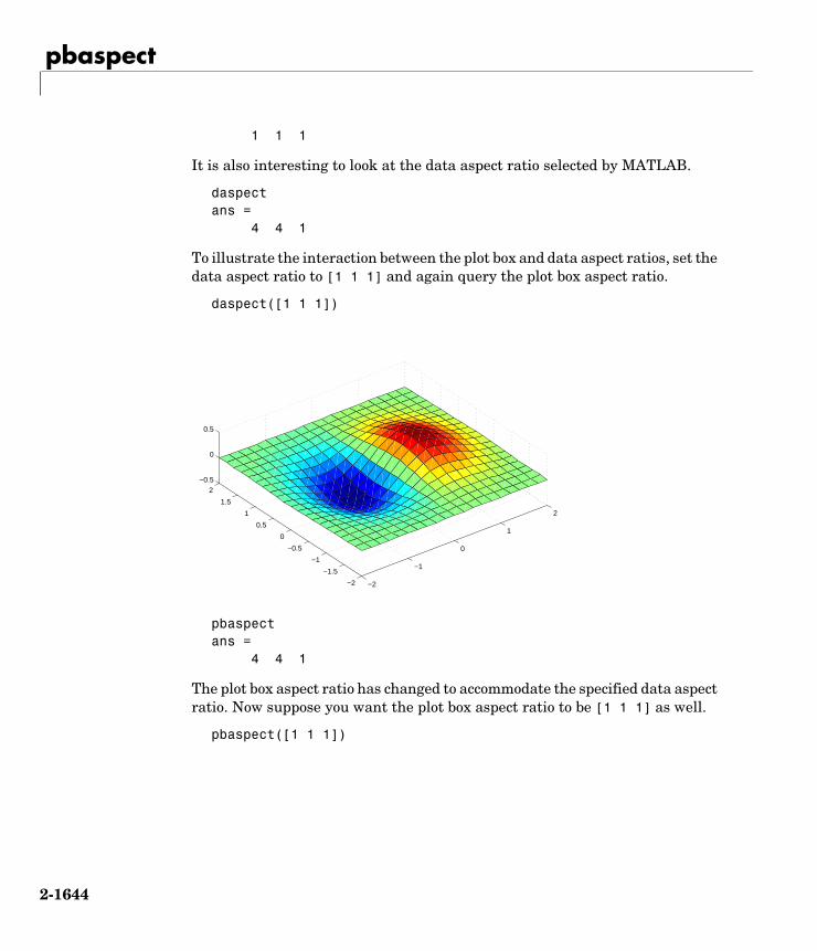
pbaspect
2-1644
1 1 1
It is also interesting to look at the data aspect ratio selected by MATLAB.
daspectans =
4 4 1
To illustrate the interaction between the plot box and data aspect ratios, set the data aspect ratio to [1 1 1] and again query the plot box aspect ratio.
daspect([1 1 1])
pbaspectans =
4 4 1
The plot box aspect ratio has changed to accommodate the specified data aspect ratio. Now suppose you want the plot box aspect ratio to be [1 1 1] as well.
pbaspect([1 1 1])
−2
−1
0
1
2
−2
−1.5
−1
−0.5
0
0.5
1
1.5
2−0.5
0
0.5

pbaspect
2-1645
Notice how MATLAB changed the axes limits because of the constraints introduced by specifying both the plot box and data aspect ratios.
You can also use pbaspect to disable stretch-to-fill. For example, displaying two subplots in one figure can give surface plots a squashed appearance. Disabling stretch-to-fill,
upper_plot = subplot(211);surf(x,y,z)lower_plot = subplot(212);surf(x,y,z)pbaspect(upper_plot,'manual')
−2
−1
0
1
2
−2
−1
0
1
2−2
−1.5
−1
−0.5
0
0.5
1
1.5
2
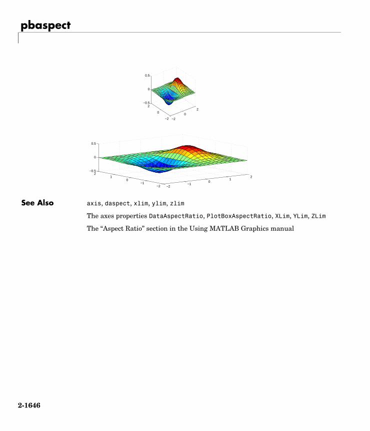
pbaspect
2-1646
See Also axis, daspect, xlim, ylim, zlim
The axes properties DataAspectRatio, PlotBoxAspectRatio, XLim, YLim, ZLim
The “Aspect Ratio” section in the Using MATLAB Graphics manual
−20
2
−2
0
2−0.5
0
0.5
−2−1
01
2
−2−1
01
2−0.5
0
0.5

pcg
2-1647
2pcgPurpose Preconditioned Conjugate Gradients method
Syntax x = pcg(A,b)pcg(A,b,tol)pcg(A,b,tol,maxit)pcg(A,b,tol,maxit,M)pcg(A,b,tol,maxit,M1,M2)pcg(A,b,tol,maxit,M1,M2,x0)pcg(A,b,tol,maxit,M1,M2,x0,p1,p2,...)[x,flag] = pcg(A,b,tol,maxit,M1,M2,x0,p1,p2,...) [x,flag,relres] = pcg(A,b,tol,maxit,M1,M2,x0,p1,p2,...)[x,flag,relres,iter] = pcg(A,b,tol,maxit,M1,M2,x0,p1,p2,...)[x,flag,relres,iter,resvec] = pcg(A,b,tol,maxit,M1,M2,x0,p1,p2,...)
Description x = pcg(A,b) attempts to solve the system of linear equations A*x=b for x. The n-by-n coefficient matrix A must be symmetric and positive definite, and should also be large and sparse. The column vector b must have length n. A can be a function afun such that afun(x) returns A*x.
If pcg converges, a message to that effect is displayed. If pcg fails to converge after the maximum number of iterations or halts for any reason, a warning message is printed displaying the relative residual norm(b-A*x)/norm(b) and the iteration number at which the method stopped or failed.
pcg(A,b,tol) specifies the tolerance of the method. If tol is [], then pcg uses the default, 1e-6.
pcg(A,b,tol,maxit) specifies the maximum number of iterations. If maxit is [], then pcg uses the default, min(n,20).
pcg(A,b,tol,maxit,M) and pcg(A,b,tol,maxit,M1,M2) use symmetric positive definite preconditioner M or M = M1*M2 and effectively solve the system inv(M)*A*x = inv(M)*b for x. If M is [] then pcg applies no preconditioner. M can be a function that returns M\x.
pcg(A,b,tol,maxit,M1,M2,x0) specifies the initial guess. If x0 is [], then pcg uses the default, an all-zero vector.

pcg
2-1648
pcg(afun,b,tol,maxit,m1fun,m2fun,x0,p1,p2,...) passes parameters p1,p2,... to functions afun(x,p1,p2,...), m1fun(x,p1,p2,...), and m2fun(x,p1,p2,...).
[x,flag] = pcg(A,b,tol,maxit,M1,M2,x0) also returns a convergence flag.
Whenever flag is not 0, the solution x returned is that with minimal norm residual computed over all the iterations. No messages are displayed if the flag output is specified.
[x,flag,relres] = pcg(A,b,tol,maxit,M1,M2,x0) also returns the relative residual norm(b-A*x)/norm(b). If flag is 0, relres <= tol.
[x,flag,relres,iter] = pcg(A,b,tol,maxit,M1,M2,x0) also returns the iteration number at which x was computed, where 0 <= iter <= maxit.
[x,flag,relres,iter,resvec] = pcg(A,b,tol,maxit,M1,M2,x0) also returns a vector of the residual norms at each iteration including norm(b-A*x0).
Examples Example 1.
A = gallery('wilk',21); b = sum(A,2);tol = 1e-12; maxit = 15; M = diag([10:-1:1 1 1:10]);
Flag Convergence
0 pcg converged to the desired tolerance tol within maxit iterations.
1 pcg iterated maxit times but did not converge.
2 Preconditioner M was ill-conditioned.
3 pcg stagnated. (Two consecutive iterates were the same.)
4 One of the scalar quantities calculated during pcg became too small or too large to continue computing.

pcg
2-1649
[x,flag,rr,iter,rv] = pcg(A,b,tol,maxit,M);
Alternatively, use this one-line matrix-vector product function
function y = afun(x,n)y = [0; x(1:n-1)] + [((n-1)/2:-1:0)'; (1:(n-1)/2)'].*x + [x(2:n); 0];
and this one-line preconditioner backsolve function
function y = mfun(r,n)y = r ./ [((n-1)/2:-1:1)'; 1; (1:(n-1)/2)'];
as inputs to pcg
[x1,flag1,rr1,iter1,rv1] = pcg(@afun,b,tol,maxit,@mfun,... [],[],21);
Example 2.
A = delsq(numgrid('C',25));b = ones(length(A),1);[x,flag] = pcg(A,b)
flag is 1 because pcg does not converge to the default tolerance of 1e-6 within the default 20 iterations.
R = cholinc(A,1e-3);[x2,flag2,relres2,iter2,resvec2] = pcg(A,b,1e-8,10,R',R)
flag2 is 0 because pcg converges to the tolerance of 1.2e-9 (the value of relres2) at the sixth iteration (the value of iter2) when preconditioned by the incomplete Cholesky factorization with a drop tolerance of 1e-3. resvec2(1) = norm(b) and resvec2(7) = norm(b-A*x2). You can follow the progress of pcg by plotting the relative residuals at each iteration starting from the initial estimate (iterate number 0).
semilogy(0:iter2,resvec2/norm(b),'-o')xlabel('iteration number')ylabel('relative residual')

pcg
2-1650
See Also bicg, bicgstab, cgs, cholinc, gmres, lsqr, minres, qmr, symmlq
@ (function handle), \ (backslash)
References [1] Barrett, R., M. Berry, T. F. Chan, et al., Templates for the Solution of Linear Systems: Building Blocks for Iterative Methods, SIAM, Philadelphia, 1994.
0 1 2 3 4 5 610
−9
10−8
10−7
10−6
10−5
10−4
10−3
10−2
10−1
100
iteration number
rela
tive
resi
dual

pchip
2-1651
2pchipPurpose Piecewise Cubic Hermite Interpolating Polynomial (PCHIP)
Syntax yi = pchip(x,y,xi)pp = pchip(x,y)
Description yi = pchip(x,y,xi) returns vector yi containing elements corresponding to the elements of xi and determined by piecewise cubic interpolation within vectors x and y. The vector x specifies the points at which the data y is given. If y is a matrix, then the interpolation is performed for each column of y and yi is length(xi)-by-size(y,2).
pp = pchip(x,y) returns a piecewise polynomial structure for use by ppval. x can be a row or column vector. y is a row or column vector of the same length as x, or a matrix with length(x) columns.
pchip finds values of an underlying interpolating function at intermediate points, such that:
• On each subinterval , is the cubic Hermite interpolant to the given values and certain slopes at the two endpoints.
• interpolates , i.e., , and the first derivative is continuous. is probably not continuous; there may be jumps at the .
• The slopes at the are chosen in such a way that preserves the shape of the data and respects monotonicity. This means that, on intervals where the data are monotonic, so is ; at points where the data has a local extremum, so does .
Note If is a matrix, satisfies the above for each column of .
Remarks spline constructs in almost the same way pchip constructs . However, spline chooses the slopes at the differently, namely to make even
continuous. This has the following effects:
• spline produces a smoother result, i.e. is continuous.
• spline produces a more accurate result if the data consists of values of a smooth function.
P x( )
xk x xk 1+≤ ≤ P x( )
P x( ) y P xj( ) yj= P ′ x( )P″ x( ) xj
xj P x( )
P x( )P x( )
y P x( ) y
S x( ) P x( )xj
S″ x( )
S″ x( )

pchip
2-1652
• pchip has no overshoots and less oscillation if the data are not smooth.
• pchip is less expensive to set up.
• The two are equally expensive to evaluate.
Examples x = -3:3; y = [-1 -1 -1 0 1 1 1]; t = -3:.01:3;p = pchip(x,y,t);s = spline(x,y,t);plot(x,y,'o',t,p,'-',t,s,'-.')legend('data','pchip','spline',4)
See Also interp1, spline, ppval
References [1] Fritsch, F. N. and R. E. Carlson, “Monotone Piecewise Cubic Interpolation,” SIAM J. Numerical Analysis, Vol. 17, 1980, pp.238-246.
[2] Kahaner, David, Cleve Moler, Stephen Nash, Numerical Methods and Software, Prentice Hall, 1988.
−3 −2 −1 0 1 2 3−1.5
−1
−0.5
0
0.5
1
1.5
datapchipspline

pcode
2-1653
2pcodePurpose Create preparsed pseudocode file (P-file)
Syntax pcode funpcode *.mpcode fun1 fun2 ...pcode... -inplace
Description pcode fun parses the M-file fun.m into the P-file fun.p and puts it into the current directory. The original M-file can be anywhere on the search path.
pcode *.m creates P-files for all the M-files in the current directory.
pcode fun1 fun2 ... creates P-files for the listed functions.
pcode... -inplace creates P-files in the same directory as the M-files. An error occurs if the files can’t be created.

pcolor
2-1654
2pcolor Purpose Pseudocolor plot
Syntax pcolor(C)pcolor(X,Y,C)pcolor(axes_handle,...)h = pcolor(...)
Description A pseudocolor plot is a rectangular array of cells with colors determined by C. MATLAB creates a pseudocolor plot using each set of four adjacent points in C to define a surface rectangle (i.e., cell).
The default shading is faceted, which colors each cell with a single color. The last row and column of C are not used in this case. With shading interp, each cell is colored by bilinear interpolation of the colors at its four vertices, using all elements of C.
The minimum and maximum elements of C are assigned the first and last colors in the colormap. Colors for the remaining elements in C are determined by a linear mapping from value to colormap element.
pcolor(C) draws a pseudocolor plot. The elements of C are linearly mapped to an index into the current colormap. The mapping from C to the current colormap is defined by colormap and caxis.
pcolor(X,Y,C) draws a pseudocolor plot of the elements of C at the locations specified by X and Y. The plot is a logically rectangular, two-dimensional grid with vertices at the points [X(i,j), Y(i,j)]. X and Y are vectors or matrices that specify the spacing of the grid lines. If X and Y are vectors, X corresponds to the columns of C and Y corresponds to the rows. If X and Y are matrices, they must be the same size as C.
pcolor(axes_handles,...) plots into the axes with handle axes_handle instead of the current axes (gca).
h = pcolor(...) returns a handle to a surface graphics object.
Remarks A pseudocolor plot is a flat surface plot viewed from above. pcolor(X,Y,C) is the same as viewing surf(X,Y,0*Z,C) using view([0 90]).

pcolor
2-1655
When you use shading faceted or shading flat, the constant color of each cell is the color associated with the corner having the smallest x-y coordinates. Therefore, C(i,j) determines the color of the cell in the ith row and jth column. The last row and column of C are not used.
When you use shading interp, each cell’s color results from a bilinear interpolation of the colors at its four vertices, and all elements of C are used.
Examples A Hadamard matrix has elements that are +1 and 1. A colormap with only two entries is appropriate when displaying a pseudocolor plot of this matrix.
pcolor(hadamard(20))colormap(gray(2))axis ijaxis square
A simple color wheel illustrates a polar coordinate system.
n = 6;r = (0:n)'/n;theta = pi*( n:n)/n;X = r*cos(theta);Y = r*sin(theta);C = r*cos(2*theta);pcolor(X,Y,C)
2 4 6 8 10 12 14 16 18 20

pcolor
2-1656
axis equal tight
Algorithm The number of vertex colors for pcolor(C) is the same as the number of cells for image(C). pcolor differs from image in that pcolor(C) specifies the colors of vertices, which are scaled to fit the colormap; changing the axes clim property changes this color mapping. image(C) specifies the colors of cells and directly indexes into the colormap without scaling. Additionally, pcolor(X,Y,C) can produce parametric grids, which is not possible with image.
See Also caxis, image, mesh, shading, surf, view
−1 −0.5 0 0.5 1−1
−0.8
−0.6
−0.4
−0.2
0
0.2
0.4
0.6
0.8
1

pdepe
2-1657
2pdepePurpose Solve initial-boundary value problems for systems of parabolic and elliptic partial differential equations (PDEs) in one space variable and time
Syntax sol = pdepe(m,pdefun,icfun,bcfun,xmesh,tspan)sol = pdepe(m,pdefun,icfun,bcfun,xmesh,tspan,options)sol = pdepe(m,pdefun,icfun,bcfun,xmesh,tspan,options,p1,p2...)
Arguments
Description sol = pdepe(m,pdefun,icfun,bcfun,xmesh,tspan) solves initial-boundary value problems for systems of parabolic and elliptic PDEs in the one space variable and time . The ordinary differential equations (ODEs) resulting from discretization in space are integrated to obtain approximate solutions at times specified in tspan. The pdepe function returns values of the solution on a mesh provided in xmesh.
m A parameter corresponding to the symmetry of the problem. m can be slab = 0, cylindrical = 1, or spherical = 2.
pdefun A function that defines the components of the PDE.
icfun A function that defines the initial conditions.
bcfun A function that defines the boundary conditions.
xmesh A vector [x0, x1, ..., xn] specifying the points at which a numerical solution is requested for every value in tspan. The elements of xmesh must satisfy x0 < x1 < ... < xn. The length of xmesh must be >= 3.
tspan A vector [t0, t1, ..., tf] specifying the points at which a solution is requested for every value in xmesh. The elements of tspan must satisfy t0 < t1 < ... < tf. The length of tspan must be >= 3.
options Some options of the underlying ODE solver are available in pdepe: RelTol, AbsTol, NormControl, InitialStep, and MaxStep. In most cases, default values for these options provide satisfactory solutions. See odeset for details.
p1,p2,... Optional parameters to be passed to pdefun, icfun, and bcfun.
x t

pdepe
2-1658
pdepe solves PDEs of the form:
(2-1)
The PDEs hold for and . The interval must be finite. can be 0, 1, or 2, corresponding to slab, cylindrical, or spherical symmetry,
respectively. If , then must be >= 0.
In Equation 2-1, is a flux term and is a source term. The coupling of the partial derivatives with respect to time is restricted to multiplication by a diagonal matrix . The diagonal elements of this matrix are either identically zero or positive. An element that is identically zero corresponds to an elliptic equation and otherwise to a parabolic equation. There must be at least one parabolic equation. An element of that corresponds to a parabolic equation can vanish at isolated values of if those values of are mesh points. Discontinuities in and/or due to material interfaces are permitted provided that a mesh point is placed at each interface.
For and all , the solution components satisfy initial conditions of the form
(2-2)
For all and either or , the solution components satisfy a boundary condition of the form
(2-3)
Elements of are either identically zero or never zero. Note that the boundary conditions are expressed in terms of the flux rather than . Also, of the two coefficients, only can depend on .
In the call sol = pdepe(m,pdefun,icfun,bcfun,xmesh,tspan):
• m corresponds to .
• xmesh(1) and xmesh(end) correspond to and .
• tspan(1) and tspan(end) correspond to and .
c x t u∂u∂x-------, , ,
∂u∂t------- x m– ∂
∂x------ xm f x t u
∂u∂x-------, , ,
s x t u
∂u∂x-------, , ,
+=
t0 t tf≤ ≤ a x b≤ ≤ a b,[ ]m
m 0> a
f x t u ∂u ∂x⁄, , ,( ) s x t u ∂u ∂x⁄, , ,( )
c x t u ∂u ∂x⁄, , ,( )
cx
x c s
t t0= x
u x t0,( ) u0 x( )=
t x a= x b=
p x t u, ,( ) q x t,( ) f x t uu∂x∂
-------, , , + 0=
qf ∂u ∂x⁄
p u
m
a b
t0 tf

pdepe
2-1659
• pdefun computes the terms , , and (Equation 2-1). It has the form [c,f,s] = pdefun(x,t,u,dudx)
The input arguments are scalars x and t and vectors u and dudx that approximate the solution and its partial derivative with respect to , respectively. c, f, and s are column vectors. c stores the diagonal elements of the matrix (Equation 2-1).
• icfun evaluates the initial conditions. It has the formu = icfun(x)
When called with an argument x, icfun evaluates and returns the initial values of the solution components at x in the column vector u.
• bcfun evaluates the terms and of the boundary conditions (Equation 2-3). It has the form [pl,ql,pr,qr] = bcfun(xl,ul,xr,ur,t)
ul is the approximate solution at the left boundary xl = and ur is the approximate solution at the right boundary xr = . pl and ql are column vectors corresponding to and evaluated at xl, similarly pr and qr correspond to xr. When and , boundedness of the solution near
requires that the flux vanish at . pdepe imposes this boundary condition automatically and it ignores values returned in pl and ql.
pdepe returns the solution as a multidimensional array sol. = ui = sol(:,:,i) is an approximation to the ith component of the solution
vector . The element ui(j,k) = sol(j,k,i) approximates at = (tspan(j),xmesh(k)).
ui = sol(j,:,i) approximates component i of the solution at time tspan(j) and mesh points xmesh(:). Use pdeval to compute the approximation and its partial derivative at points not included in xmesh. See pdeval for details.
sol = pdepe(m,pdefun,icfun,bcfun,xmesh,tspan,options) solves as above with default integration parameters replaced by values in options, an argument created with the odeset function. Only some of the options of the underlying ODE solver are available in pdepe: RelTol, AbsTol, NormControl,
c f s
u x
c
p q
ab
p qm 0> a 0=
x 0= f a 0=
uiu ui
t x,( )
∂ui ∂x⁄

pdepe
2-1660
InitialStep, and MaxStep. The defaults obtained by leaving off the input argument options will generally be satisfactory. See odeset for details.
sol = pdepe(m,pdefun,icfun,bcfun,xmesh,tspan,options,p1,p2...)passes the additional parameters p1, p2, ... to the functions pdefun, icfun, and bcfun. Use options = [] as a placeholder if no options are set.
Remarks • The arrays xmesh and tspan play different roles in pdepe.
tspan The pdepe function performs the time integration with an ODE solver that selects both the time step and formula dynamically. The elements of tspan merely specify where you want answers and the cost depends weakly on the length of tspan.
xmesh Second order approximations to the solution are made on the mesh specified in xmesh. Generally, it is best to use closely spaced mesh points where the solution changes rapidly. pdepe does not select the mesh in automatically. You must provide an appropriate fixed mesh in xmesh. The cost depends strongly on the length of xmesh. When , it is not necessary to use a fine mesh near to account for the coordinate singularity.
• The time integration is done with ode15s. pdepe exploits the capabilities of ode15s for solving the differential-algebraic equations that arise when Equation 2-1 contains elliptic equations, and for handling Jacobians with a specified sparsity pattern.
• After discretization, elliptic equations give rise to algebraic equations. If the elements of the initial conditions vector that correspond to elliptic equations are not “consistent” with the discretization, pdepe tries to adjust them before beginning the time integration. For this reason, the solution returned for the initial time may have a discretization error comparable to that at any other time. If the mesh is sufficiently fine, pdepe can find consistent initial conditions close to the given ones. If pdepe displays a message that it has difficulty finding consistent initial conditions, try refining the mesh.
No adjustment is necessary for elements of the initial conditions vector that correspond to parabolic equations.
x
m 0>x 0=

pdepe
2-1661
Examples Example 1. This example illustrates the straightforward formulation, computation, and plotting of the solution of a single PDE.
This equation holds on an interval for times .
The PDE satisfies the initial condition
and boundary conditions
It is convenient to use subfunctions to place all the functions required by pdepe in a single M-file.
function pdex1
m = 0;x = linspace(0,1,20);t = linspace(0,2,5);
sol = pdepe(m,@pdex1pde,@pdex1ic,@pdex1bc,x,t);% Extract the first solution component as u.u = sol(:,:,1);
% A surface plot is often a good way to study a solution.surf(x,t,u) title('Numerical solution computed with 20 mesh points.')xlabel('Distance x')ylabel('Time t')
% A solution profile can also be illuminating.figureplot(x,u(end,:))title('Solution at t = 2')xlabel('Distance x')
π2 ∂u∂t------ ∂
∂x------ ∂u
∂x------ =
0 x 1≤ ≤ t 0≥
u x 0,( ) πxsin=
u 0 t,( ) 0≡
πe t– ∂u∂x------ 1 t,( )+ 0=

pdepe
2-1662
ylabel('u(x,2)')% --------------------------------------------------------------function [c,f,s] = pdex1pde(x,t,u,DuDx)c = pi^2;f = DuDx;s = 0;% --------------------------------------------------------------function u0 = pdex1ic(x)u0 = sin(pi*x);% --------------------------------------------------------------function [pl,ql,pr,qr] = pdex1bc(xl,ul,xr,ur,t)pl = ul;ql = 0;pr = pi * exp(-t);qr = 1;
In this example, the PDE, initial condition, and boundary conditions are coded in subfunctions pdex1pde, pdex1ic, and pdex1bc.
The surface plot shows the behavior of the solution.
00.2
0.40.6
0.81
0
0.5
1
1.5
20
0.2
0.4
0.6
0.8
1
Distance x
Numerical solution computed with 20 mesh points.
Time t

pdepe
2-1663
The following plot shows the solution profile at the final value of t (i.e., t = 2).
Example 2. This example illustrates the solution of a system of PDEs. The problem has boundary layers at both ends of the interval. The solution changes rapidly for small .
The PDEs are
where .
This equation holds on an interval for times .
0 0.1 0.2 0.3 0.4 0.5 0.6 0.7 0.8 0.9 1−0.02
0
0.02
0.04
0.06
0.08
0.1
0.12
0.14Solution at t = 2
Distance x
u(x,
2)
t
∂u1∂t
--------- 0.024∂2u1
∂x2------------ F u1 u2–( )–=
∂u2∂t
--------- 0.170∂2u2
∂x2------------ F u1 u2–( )+=
F y( ) exp 5.73y( ) exp 11.46– y( )–=
0 x 1≤ ≤ t 0≥

pdepe
2-1664
The PDE satisfies the initial conditions
and boundary conditions
In the form expected by pdepe, the equations are
The boundary conditions on the partial derivatives of have to be written in terms of the flux. In the form expected by pdepe, the left boundary condition is
and the right boundary condition is
The solution changes rapidly for small . The program selects the step size in time to resolve this sharp change, but to see this behavior in the plots, the example must select the output times accordingly. There are boundary layers in the solution at both ends of [0,1], so the example places mesh points near 0 and 1 to resolve these sharp changes. Often some experimentation is needed to select a mesh that reveals the behavior of the solution.
u1 x 0,( ) 1≡
u2 x 0,( ) 0≡
∂u1∂x
--------- 0 t,( ) 0≡
u2 0 t,( ) 0≡
u1 1 t,( ) 1≡
∂u2∂x
--------- 1 t,( ) 0≡
1
1
∂∂t-----
u1
u2
∂∂x------
0.024 ∂u1 ∂x⁄( )
0.170 ∂u2 ∂x⁄( )
F u1 u2–( )–
F u1 u2–( )+=.∗
u
0u2
1
0+
0.024 ∂u1 ∂x⁄( )
0.170 ∂u2 ∂x⁄( )
0
0=.∗
u1 1–
0
0
1+
0.024 ∂u1 ∂x⁄( )
0.170 ∂u2 ∂x⁄( )0
0=.∗
t

pdepe
2-1665
function pdex4m = 0;x = [0 0.005 0.01 0.05 0.1 0.2 0.5 0.7 0.9 0.95 0.99 0.995 1];t = [0 0.005 0.01 0.05 0.1 0.5 1 1.5 2];
sol = pdepe(m,@pdex4pde,@pdex4ic,@pdex4bc,x,t);u1 = sol(:,:,1);u2 = sol(:,:,2);
figuresurf(x,t,u1)title('u1(x,t)')xlabel('Distance x')ylabel('Time t')
figuresurf(x,t,u2)title('u2(x,t)')xlabel('Distance x')ylabel('Time t')% --------------------------------------------------------------function [c,f,s] = pdex4pde(x,t,u,DuDx)c = [1; 1]; f = [0.024; 0.17] .* DuDx; y = u(1) - u(2);F = exp(5.73*y)-exp(-11.47*y);s = [-F; F]; % --------------------------------------------------------------function u0 = pdex4ic(x);u0 = [1; 0]; % --------------------------------------------------------------function [pl,ql,pr,qr] = pdex4bc(xl,ul,xr,ur,t)pl = [0; ul(2)]; ql = [1; 0]; pr = [ur(1)-1; 0]; qr = [0; 1];
In this example, the PDEs, intial conditions, and boundary conditions are coded in subfunctions pdex4pde, pdex4ic, and pdex4bc.

pdepe
2-1666
The surface plots show the behavior of the solution components.
00.2
0.40.6
0.81
0
0.5
1
1.5
20
0.2
0.4
0.6
0.8
1
Distance x
u1(x,t)
Time t
00.2
0.40.6
0.81
0
0.5
1
1.5
20
0.1
0.2
0.3
0.4
0.5
0.6
0.7
0.8
Distance x
u2(x,t)
Time t

pdepe
2-1667
See Also function_handle, pdeval, ode15s, odeset, odeget
References [1] Skeel, R. D. and M. Berzins, “A Method for the Spatial Discretization of Parabolic Equations in One Space Variable,” SIAM Journal on Scientific and Statistical Computing, Vol. 11, 1990, pp.1-32.

pdeval
2-1668
2pdevalPurpose Evaluate the numerical solution of a PDE using the output of pdepe
Syntax [uout,duoutdx] = pdeval(m,xmesh,ui,xout)
Arguments
Description [uout,duoutdx] = pdeval(m,x,ui,xout) approximates the solution and its partial derivative at points from the interval [x0,xn]. The pdeval function returns the computed values in uout and duoutdx, respectively.
Note pdeval evaluates the partial derivative rather than the flux . Although the flux is continuous, the partial derivative may have a jump at a material interface.
See Also pdepe
m Symmetry of the problem: slab = 0, cylindrical = 1, spherical = 2. This is the first input argument used in the call to pdepe.
xmesh A vector [x0, x1, ..., xn] specifying the points at which the elements of ui were computed. This is the same vector with which pdepe was called.
ui A vector sol(j,:,i) that approximates component i of the solution at time and mesh points xmesh, where sol is the solution returned by pdepe.
xout A vector of points from the interval [x0,xn] at which the interpolated solution is requested.
tf
ui∂ui ∂x⁄
∂ui ∂x⁄ f

peaks
2-1669
2peaksPurpose A sample function of two variables.
Syntax Z = peaks;Z = peaks(n);Z = peaks(V);Z = peaks(X,Y); peaks;peaks(N);peaks(V);peaks(X,Y); [X,Y,Z] = peaks;[X,Y,Z] = peaks(n);[X,Y,Z] = peaks(V);
Description peaks is a function of two variables, obtained by translating and scaling Gaussian distributions, which is useful for demonstrating mesh, surf, pcolor, contour, and so on.
Z = peaks; returns a 49-by-49 matrix.
Z = peaks(n); returns an n-by-n matrix.
Z = peaks(V); returns an n-by-n matrix, where n = length(V).
Z = peaks(X,Y); evaluates peaks at the given X and Y (which must be the same size) and returns a matrix the same size.
peaks(...) (with no output argument) plots the peaks function with surf.
[X,Y,Z] = peaks(...); returns two additional matrices, X and Y, for parametric plots, for example, surf(X,Y,Z,del2(Z)). If not given as input, the underlying matrices X and Y are
[X,Y] = meshgrid(V,V)
where V is a given vector, or V is a vector of length n with elements equally spaced from −3 to 3. If no input argument is given, the default n is 49.
See Also meshgrid, surf

perl
2-1670
2perlPurpose Call Perl script using appropriate operating system executable
Syntax perl('perlfile')perl('perlfile',arg1,arg2,...)result = perl(...)
Description perl('perlfile') calls the Perl script perlfile, using the appropriate oper-ating system Perl executable. Perl is included with MATLAB, so MATLAB users can run M-files containing the perl function.
perl('perlfile',arg1,arg2,...) calls the Perl script perlfile, using the appropriate operating system Perl executable, and passes the arguments arg1, arg2, and so on, to perlfile.
result = perl(...) returns the results of attempted Perl call to result.
Examples Given the Perl script, hello.pl
$input = $ARGV[0]; print "Hello $input.";
run the following statement in MATLAB
perl('hello.pl','World')
MATLAB returns
ans =Hello World.
It is sometimes beneficial to use Perl scripts instead of MATLAB code. The perl function allows you to run those scripts from within MATLAB. Specific examples where you might choose to use a Perl script include:
• Perl script already exists
• Perl script preprocesses data quickly, formatting it in a way more easily read by MATLAB
• Perl has features not supported by MATLAB
See Also ! (exclamation point), dos, regexp, system, unix

perms
2-1671
2permsPurpose All possible permutations
Syntax P = perms(v)
Description P = perms(v), where v is a row vector of length n, creates a matrix whose rows consist of all possible permutations of the n elements of v. Matrix P contains n! rows and n columns.
Examples The command perms(2:2:6) returns all the permutations of the numbers 2, 4, and 6:
6 4 2 6 2 4 4 6 2 4 2 6 2 4 6 2 6 4
Limitations This function is only practical for situations where n is less than about 15.
See Also nchoosek, permute, randperm

permute
2-1672
2permutePurpose Rearrange the dimensions of a multidimensional array
Syntax B = permute(A,order)
Description B = permute(A,order) rearranges the dimensions of A so that they are in the order specified by the vector order. B has the same values of A but the order of the subscripts needed to access any particular element is rearranged as specified by order. All the elements of order must be unique.
Remarks permute and ipermute are a generalization of transpose (.') for multidimensional arrays.
Examples Given any matrix A, the statement
permute(A,[2 1])
is the same as A'.
For example:
A = [1 2; 3 4]; permute(A,[2 1])ans = 1 3 2 4
The following code permutes a three-dimensional array:
X = rand(12,13,14);Y = permute(X,[2 3 1]);size(Y)ans = 13 14 12
See Also ipermute

persistent
2-1673
2persistentPurpose Define persistent variable
Syntax persistent X Y Z
Description persistent X Y Z defines X, Y, and Z as variables that are local to the function in which they are declared; yet their values are retained in memory between calls to the function. Persistent variables are similar to global variables because MATLAB creates permanent storage for both. They differ from global variables in that persistent variables are known only to the function in which they are declared. This prevents persistent variables from being changed by other functions or from the MATLAB command line.
Persistent variables are cleared when the M-file is cleared from memory or when the M-file is changed. To keep an M-file in memory until MATLAB quits, use mlock.
If the persistent variable does not exist the first time you issue the persistent statement, it is initialized to the empty matrix.
It is an error to declare a variable persistent if a variable with the same name exists in the current workspace.
Remarks There is no function form of the persistent command (i.e., you cannot use parentheses and quote the variable names).
See Also clear, global, mislocked, mlock, munlock

pi
2-1674
2piPurpose Ratio of a circle’s circumference to its diameter,
Syntax pi
Description pi returns the floating-point number nearest the value of . The expressions 4*atan(1) and imag(log(-1)) provide the same value.
Examples The expression sin(pi) is not exactly zero because pi is not exactly .
sin(pi)
ans =
1.2246e-16
See Also ans, eps, i, Inf, j, NaN
π
π
π

pie
2-1675
2piePurpose Pie chart
Syntax pie(X)pie(X,explode)pie(...,labels)pie(axes_handle,...)h = pie(...)
Description pie(X) draws a pie chart using the data in X. Each element in X is represented as a slice in the pie chart.
pie(X,explode) offsets a slice from the pie. explode is a vector or matrix of zeros and nonzeros that correspond to X. A nonzero value offsets the corresponding slice from the center of the pie chart, so that X(i,j) is offset from the center if explode(i,j) is nonzero. explode must be the same size as X.
pie(...,labels) specifies text labels for the slices. The number of labels must equal the number of elements in X. For example,
pie(1:3,'Taxes','Expenses','Profit')
pie(axes_handle,...) plots into the axes with handle axes_handle instead of the current axes (gca).
h = pie(...) returns a vector of handles to patch and text graphics objects.
Remarks The values in X are normalized via X/sum(X) to determine the area of each slice of the pie. If sum(X)≤1, the values in X directly specify the area of the pie slices. MATLAB draws only a partial pie if sum(X)<1.
Examples Emphasize the second slice in the chart by setting its corresponding explode element to 1.
x = [1 3 0.5 2.5 2];explode = [0 1 0 0 0];pie(x,explode)colormap jet

pie
2-1676
See Also pie3
11%
33%
6%
28%
22%

pie3
2-1677
2pie3Purpose Three-dimensional pie chart
Syntax pie3(X)pie3(X,explode)pie3(...,labels)pie3(axes_handle,...)h = pie3(...)
Description pie3(X) draws a three-dimensional pie chart using the data in X. Each element in X is represented as a slice in the pie chart.
pie3(X,explode) specifies whether to offset a slice from the center of the pie chart. X(i,j) is offset from the center of the pie chart if explode(i,j) is nonzero. explode must be the same size as X.
pie3(...,labels) specifies text labels for the slices. The number of labels must equal the number of elements in X. For example,
pie3(1:3,'Taxes','Expenses','Profit')
pie3(axes_handle,...) plots into the axes with handle axes_handle instead of the current axes (gca).
h = pie(...) returns a vector of handles to patch, surface, and text graphics objects.
Remarks The values in X are normalized via X/sum(X) to determine the area of each slice of the pie. If sum(X)≤1, the values in X directly specify the area of the pie slices. MATLAB draws only a partial pie if sum(X)<1.
Examples Offset a slice in the pie chart by setting the corresponding explode element to 1:
x = [1 3 0.5 2.5 2]explode = [0 1 0 0 0]pie3(x,explode)colormap hsv

pie3
2-1678
See Also pie
28%
6%
22%
33%
11%

pinv
2-1679
2pinvPurpose Moore-Penrose pseudoinverse of a matrix
Syntax B = pinv(A)B = pinv(A,tol)
Definition The Moore-Penrose pseudoinverse is a matrix B of the same dimensions as A' satisfying four conditions:
A*B*A = AB*A*B = BA*B is HermitianB*A is Hermitian
The computation is based on svd(A) and any singular values less than tol are treated as zero.
Description B = pinv(A) returns the Moore-Penrose pseudoinverse of A.
B = pinv(A,tol) returns the Moore-Penrose pseudoinverse and overrides the default tolerance, max(size(A))*norm(A)*eps.
Examples If A is square and not singular, then pinv(A) is an expensive way to compute inv(A). If A is not square, or is square and singular, then inv(A) does not exist. In these cases, pinv(A) has some of, but not all, the properties of inv(A).
If A has more rows than columns and is not of full rank, then the overdetermined least squares problem
minimize norm(A*x-b)
does not have a unique solution. Two of the infinitely many solutions are
x = pinv(A)*b
and
y = A\b
These two are distinguished by the facts that norm(x) is smaller than the norm of any other solution and that y has the fewest possible nonzero components.
For example, the matrix generated by

pinv
2-1680
A = magic(8); A = A(:,1:6)
is an 8-by-6 matrix that happens to have rank(A) = 3.
A =64 2 3 61 60 69 55 54 12 13 5117 47 46 20 21 4340 26 27 37 36 3032 34 35 29 28 3841 23 22 44 45 1949 15 14 52 53 118 58 59 5 4 62
The right-hand side is b = 260*ones(8,1),
b =260260260260260260260260
The scale factor 260 is the 8-by-8 magic sum. With all eight columns, one solution to A*x = b would be a vector of all 1’s. With only six columns, the equations are still consistent, so a solution exists, but it is not all 1’s. Since the matrix is rank deficient, there are infinitely many solutions. Two of them are
x = pinv(A)*b
which is
x =1.15381.46151.38461.38461.46151.1538

pinv
2-1681
and
y = A\b
which produces this result.
Warning: Rank deficient, rank = 3 tol = 1.8829e-013.y = 4.0000 5.0000 0 0 0 -1.0000
Both of these are exact solutions in the sense that norm(A∗ x-b) and norm(A∗ y-b) are on the order of roundoff error. The solution x is special because
norm(x) = 3.2817
is smaller than the norm of any other solution, including
norm(y) = 6.4807
On the other hand, the solution y is special because it has only three nonzero components.
See Also inv, qr, rank, svd

planerot
2-1682
2planerotPurpose Givens plane rotation
Syntax [G,y] = planerot(x)
Description [G,y] = planerot(x) where x is a 2-component column vector, returns a 2-by-2 orthogonal matrix G so that y = G*x has y(2) = 0.
Examples x = [3 4];[G,y] = planerot(x')
G = 0.6000 0.8000 -0.8000 0.6000
y = 5 0
See Also qrdelete, qrinsert

playshow
2-1683
2playshowPurpose Run published M-file demo
Syntax playshow demoname
Description playshow runs the published M-file demo demoname. To determine if a demo is a published M-file type, view the H1 line for the demo M-file, that is, the first comment line. If it begins with two comment symbols (%%), it is a published M-file demo.
Examples The first line in nesteddemo begins with two comment symbols:
%% Nested Function Examples
Therefore, type playshow nesteddemo to run the demo.
See Also demo, helpbrowser

plot
2-1684
2plotPurpose Linear 2-D plot
Syntax plot(Y)plot(X1,Y1,...)plot(X1,Y1,LineSpec,...)plot(...,'PropertyName',PropertyValue,...)plot(axes_handle,...)h = plot(...)hlines = plot('v6',...)
Description plot(Y) plots the columns of Y versus their index if Y is a real number. If Y is complex, plot(Y) is equivalent to plot(real(Y),imag(Y)). In all other uses of plot, the imaginary component is ignored.
plot(X1,Y1,...) plots all lines defined by Xn versus Yn pairs. If only Xn or Yn is a matrix, the vector is plotted versus the rows or columns of the matrix, depending on whether the vector’s row or column dimension matches the matrix.
plot(X1,Y1,LineSpec,...) plots all lines defined by the Xn,Yn,LineSpec triples, where LineSpec is a line specification that determines line type, marker symbol, and color of the plotted lines. You can mix Xn,Yn,LineSpec triples with Xn,Yn pairs: plot(X1,Y1,X2,Y2,LineSpec,X3,Y3).
Note See LineSpec for a list of line style, marker, and color specifiers.
plot(...,'PropertyName',PropertyValue,...) sets properties to the specified property values for all lineseries graphics objects created by plot. (See the “Examples” section for examples.)
plot(axes_handle,...) plots into the axes with handle axes_handle instead of the current axes (gca).
h = plot(...) returns a column vector of handles to lineseries graphics objects, one handle per line.

plot
2-1685
Backward Compatible Version
hlines = plot('v6',...) returns the handles to line objects instead of lineseries objects.
Remarks If you do not specify a color when plotting more than one line, plot automatically cycles through the colors in the order specified by the current axes ColorOrder property. After cycling through all the colors defined by ColorOrder, plot then cycles through the line styles defined in the axes LineStyleOrder property.
The default LineStyleOrder property has a single entry (a solid line with no marker).
Cycling Through Line Colors and StylesBy default, MATLAB resets the ColorOrder and LineStyleOrder properties each time you call plot. If you want changes you make to these properties to persist, then you must define these changes as default values. For example,
set(0,'DefaultAxesColorOrder',[0 0 0],...'DefaultAxesLineStyleOrder','-|-.|--|:')
sets the default ColorOrder to use only the color black and sets the LineStyleOrder to use solid, dash-dot, dash-dash, and dotted line styles.
Prevent Resetting of Color and Styles with hold allThe all option to the hold command prevents the ColorOrder and LineStyleOrder from being reset in subsequent plot commands. In the following sequence of commands, MATLAB continues to cycle through the colors defined by the axes ColorOrder property (see above).
plot(rand(12,2))hold allplot(randn(12,2))
Additional Information
• See Creating Line Plots and Annotating Graphs for more information on plotting.
• See LineSpec for more information on specifying line styles and colors.

plot
2-1686
Examples Specifying the Color and Size of MarkersYou can also specify other line characteristics using graphics properties (see line for a description of these properties):
• LineWidth — Specifies the width (in points) of the line.
• MarkerEdgeColor — Specifies the color of the marker or the edge color for filled markers (circle, square, diamond, pentagram, hexagram, and the four triangles).
• MarkerFaceColor — Specifies the color of the face of filled markers.
• MarkerSize — Specifies the size of the marker in units of points.
For example, these statements,
x = -pi:pi/10:pi;y = tan(sin(x)) - sin(tan(x));plot(x,y,'--rs','LineWidth',2,... 'MarkerEdgeColor','k',... 'MarkerFaceColor','g',... 'MarkerSize',10)
produce this graph.

plot
2-1687
Specifying Tick-Mark Location and LabelingYou can adjust the axis tick-mark locations and the labels appearing at each tick. For example, this plot of the sine function relabels the x-axis with more meaningful values:
x = -pi:.1:pi;y = sin(x);plot(x,y)set(gca,'XTick',-pi:pi/2:pi)set(gca,'XTickLabel','-pi','-pi/2','0','pi/2','pi')
Now add axis labels and annotate the point −pi/4, sin(−pi/4).
−4 −3 −2 −1 0 1 2 3 4−3
−2
−1
0
1
2
3

plot
2-1688
Adding Titles, Axis Labels, and AnnotationsMATLAB enables you to add axis labels and titles. For example, using the graph from the previous example, add an x- and y-axis label:
xlabel('-\pi \leq \Theta \leq \pi')ylabel('sin(\Theta)')title('Plot of sin(\Theta)')text(-pi/4,sin(-pi/4),'\leftarrow sin(-\pi\div4)',...
'HorizontalAlignment','left')
Now change the line color to red by first finding the handle of the line object created by plot and then setting its Color property. In the same statement, set the LineWidth property to 2 points.
set(findobj(gca,'Type','line','Color',[0 0 1]),...'Color','red',...
'LineWidth',2)
−pi −pi/2 0 pi/2 pi−1
−0.8
−0.6
−0.4
−0.2
0
0.2
0.4
0.6
0.8
1

plot
2-1689
See Also axis, bar, grid, hold, legend, line, LineSpec, loglog, plot3, plotyy, semilogx, semilogy, subplot, title, xlabel, xlim, ylabel, ylim, zlabel, zlim, stem
See the text String property for a list of symbols and how to display them.
See the Plot Editor for information on plot annotation tools in the figure window toolbar.
See Basic Plots and Graphs for related functions.
−pi −pi/2 0 pi/2 pi−1
−0.8
−0.6
−0.4
−0.2
0
0.2
0.4
0.6
0.8
1
−π ≤ Θ ≤ π
sin(Θ
)
Plot of sin(Θ)
← sin(−π÷4)

plot3
2-1690
2plot3Purpose 3-D line plot
Syntax plot3(X1,Y1,Z1,...)plot3(X1,Y1,Z1,LineSpec,...)plot3(...,'PropertyName',PropertyValue,...)h = plot3(...)
Description The plot3 function displays a three-dimensional plot of a set of data points.
plot3(X1,Y1,Z1,...), where X1, Y1, Z1 are vectors or matrices, plots one or more lines in three-dimensional space through the points whose coordinates are the elements of X1, Y1, and Z1.
plot3(X1,Y1,Z1,LineSpec,...) creates and displays all lines defined by the Xn,Yn,Zn,LineSpec quads, where LineSpec is a line specification that determines line style, marker symbol, and color of the plotted lines.
plot3(...,'PropertyName',PropertyValue,...) sets properties to the specified property values for all line graphics objects created by plot3.
h = plot3(...) returns a column vector of handles to lineseries graphics objects, with one handle per object.
Remarks If one or more of X1, Y1, Z1 is a vector, the vectors are plotted versus the rows or columns of the matrix, depending whether the vectors’ lengths equal the number of rows or the number of columns.
You can mix Xn,Yn,Zn triples with Xn,Yn,Zn,LineSpec quads, for example,
plot3(X1,Y1,Z1,X2,Y2,Z2,LineSpec,X3,Y3,Z3)
See LineSpec and plot for information on line types and markers.
Examples Plot a three-dimensional helix.
t = 0:pi/50:10*pi;plot3(sin(t),cos(t),t)grid onaxis square

plot3
2-1691
See Also axis, bar3, grid, line, LineSpec, loglog, plot, semilogx, semilogy, subplot
−1
−0.5
0
0.5
1
−1
−0.5
0
0.5
10
5
10
15
20
25
30
35

plotbrowser
2-1692
2plotbrowserPurpose Show or hide figure plotbrowser
Syntax plotbrowser('on')plotbrowser('off')plotbrowser('toggle')plotbrowser(figure_handle,...)
Description plotbrowser('on') displays the Plot Browser on the current figure.
plotbrowser('off') hides the Plot Browser on the current figure.
plotbrowser('toggle') or plotbrowser toggles the visibility of the Plot Browser on the current figure.
plotbrowser(figure_handle,...) shows or hides the Plot Browser on the figure specified by figure_handle.
See Also figurepalette, propertyeditor

plotedit
2-1693
2ploteditPurpose Start plot edit mode to allow editing and annotation of plots
Syntax plotedit onplotedit offploteditplotedit('state')plotedit(h)plotedit(h,'state')
Description plotedit on starts plot edit mode for the current figure, allowing you to use a graphical interface to annotate and edit plots easily. In plot edit mode, you can label axes, change line styles, and add text, line, and arrow annotations.
plotedit off ends plot mode for the current figure.
plotedit toggles the plot edit mode for the current figure.
plotedit(h) toggles the plot edit mode for the figure specified by figure handle h.
plotedit('state') specifies the plotedit state for the current figure. Values for state can be as shown.
Note hidetoolsmenu is intended for GUI developers who do not want the Tools menu to appear in applications that use the figure window.
plotedit(h,'state') specifies the plotedit state for figure handle h.
Value for state Description
on Starts plot edit mode
off Ends plot edit mode
showtoolsmenu Displays the Tools menu in the menu bar
hidetoolsmenu Removes the Tools menu from the menu bar

plotedit
2-1694
Remarks Plot Editing Mode Graphical Interface Components
Examples Start plot edit mode for figure 2.
plotedit(2)
End plot edit mode for figure 2.
plotedit(2, 'off')
Hide the Tools menu for the current figure:
plotedit('hidetoolsmenu')
See Also axes, line, open, plot, print, saveas, text, propedit
To start plot edit mode, click this button.
Use these toolbar buttons to add a legend, text, and arrows.
Use the Edit, Insert, and Tools menus to add objects or edit existing objects in a
Access object-specific plot edit functions through context-sensitive pop-up menus.
Position labels, legends, and other objects by clicking and dragging.
Double-click on an object to select it.

plotedit
2-1695

plotmatrix
2-1696
2plotmatrixPurpose Draw scatter plots
Syntax plotmatrix(X,Y)plotmatrix(...,'LineSpec')[H,AX,BigAx,P] = plotmatrix(...)
Description plotmatrix(X,Y) scatter plots the columns of X against the columns of Y. If X is p-by-m and Y is p-by-n, plotmatrix produces an n-by-m matrix of axes. plotmatrix(Y) is the same as plotmatrix(Y,Y) except that the diagonal is replaced by hist(Y(:,i)).
plotmatrix(...,'LineSpec') uses a LineSpec to create the scatter plot. The default is '.'.
[H,AX,BigAx,P] = plotmatrix(...) returns a matrix of handles to the objects created in H, a matrix of handles to the individual subaxes in AX, a handle to a big (invisible) axes that frames the subaxes in BigAx, and a matrix of handles for the histogram plots in P. BigAx is left as the current axes so that a subsequent title, xlabel, or ylabel command is centered with respect to the matrix of axes.
Examples Generate plots of random data.
x = randn(50,3); y = x*[-1 2 1;2 0 1;1 -2 3;]';plotmatrix(y,'*r')
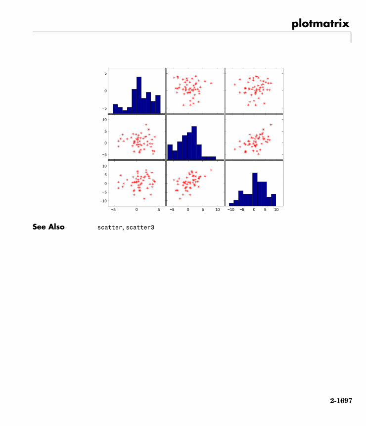
plotmatrix
2-1697
See Also scatter, scatter3
−10 −5 0 5 10−5 0 5 10−5 0 5
−10
−5
0
5
10
−5
0
5
10
−5
0
5

plottools
2-1698
2plottoolsPurpose Show or hide the plot tools
Syntax plottools('on')plottools('off')plottoolsplottools(figure_handle,...)plottools(...,'tool')
Description plottools('on') displays the Figure Palette, Plot Browser, and Property Editor on the current figure.
plottools('off') hides the Figure Palette, Plot Browser, and Property Editor on the current figure.
plottools with no arguments, is the same as plottools('on')
plottools(figure_handle,...) displays or hides the plot tools on the specified figure instead of the current figure.
plottools(...,'tool') operates on the specified tool only. tool can be one of the following strings:
• figurepalette• plotbrowser• propertyeditor
See Also figurepalette, plotbrowser, propertyeditor

plotyy
2-1699
2plotyyPurpose Create graphs with y-axes on both left and right side
Syntax plotyy(X1,Y1,X2,Y2)plotyy(X1,Y1,X2,Y2,'function')plotyy(X1,Y1,X2,Y2,'function1','function2')[AX,H1,H2] = plotyy(...)
Description plotyy(X1,Y1,X2,Y2) plots X1 versus Y1 with y-axis labeling on the left and plots X2 versus Y2 with y-axis labeling on the right.
plotyy(X1,Y1,X2,Y2,function) uses the specified plotting function to produce the graph.
function can be either a function handle or a string specifying plot, semilogx, semilogy, loglog, stem, or any MATLAB function that accepts the syntax
h = function(x,y)
For example,
plotyy(x1,y1,x2,y2,@loglog) % function handleplotyyx1,y1,x2,y2,'loglog') % string
Function handles enable you to access user-defined subfunctions and can provide other advantages. See @ for more information on using function handles.
plotyy(X1,Y1,X2,Y2,'function1','function2') uses function1(X1,Y1) to plot the data for the left axis and function2(X2,Y2) to plot the data for the right axis.
[AX,H1,H2] = plotyy(...) returns the handles of the two axes created in AX and the handles of the graphics objects from each plot in H1 and H2. AX(1) is the left axes and AX(2) is the right axes.
Examples This example graphs two mathematical functions using plot as the plotting function. The two y-axes enable you to display both sets of data on one graph even though relative values of the data are quite different.
x = 0:0.01:20;y1 = 200*exp(-0.05*x).*sin(x);

plotyy
2-1700
y2 = 0.8*exp(-0.5*x).*sin(10*x);[AX,H1,H2] = plotyy(x,y1,x,y2,'plot');
You can use the handles returned by plotyy to label the axes and set the line styles used for plotting. With the axes handles you can specify the YLabel properties of the left- and right-side y-axis:
set(get(AX(1),'Ylabel'),'String','Left Y-axis')set(get(AX(2),'Ylabel'),'String','Right Y-axis')
Use the xlabel and title commands to label the x-axis and add a title:
xlabel('Zero to 20 \musec.')title('Labeling plotyy')
Use the line handles to set the LineStyle properties of the left- and right-side plots:
set(H1,'LineStyle','--')set(H2,'LineStyle',':')
0 5 10 15 20−200
−150
−100
−50
0
50
100
150
200
Left
Y−
axis
Zero to 20 µsec.
Labeling plotyy
0 5 10 15 20−0.8
−0.6
−0.4
−0.2
0
0.2
0.4
0.6
0.8
Rig
ht Y
−ax
is

plotyy
2-1701
See Also plot, loglog, semilogx, semilogy, axes properties XAxisLocation, YAxisLocation
See Using Multiple X- and Y-Axes for more information.

pol2cart
2-1702
2pol2cartPurpose Transform polar or cylindrical coordinates to Cartesian
Syntax [X,Y] = pol2cart(THETA,RHO)[X,Y,Z] = pol2cart(THETA,RHO,Z)
Description [X,Y] = pol2cart(THETA,RHO) transforms the polar coordinate data stored in corresponding elements of THETA and RHO to two-dimensional Cartesian, or xy, coordinates. The arrays THETA and RHO must be the same size (or either can be scalar). The values in THETA must be in radians.
[X,Y,Z] = pol2cart(THETA,RHO,Z) transforms the cylindrical coordinate data stored in corresponding elements of THETA, RHO, and Z to three-dimensional Cartesian, or xyz, coordinates. The arrays THETA , RHO, and Z must be the same size (or any can be scalar). The values in THETA must be in radians.
Algorithm The mapping from polar and cylindrical coordinates to Cartesian coordinates is:
See Also cart2pol, cart2sph, sph2cart
theta = atan2(y,x)rho = sqrt(x.^2 + y.^2)
Cylindrical to Cartesian Mapping
Z
Y
X
rhotheta
P
z
Polar to Cartesian Mapping
P
X
Y
rho
theta
theta = atan2(y,x)rho = sqrt(x.^2 + y.^2)
z = z

polar
2-1703
2polarPurpose Plot polar coordinates
Syntax polar(theta,rho)polar(theta,rho,LineSpec)polar(axes_handle,...)h = polar(...)
Description The polar function accepts polar coordinates, plots them in a Cartesian plane, and draws the polar grid on the plane.
polar(theta,rho) creates a polar coordinate plot of the angle theta versus the radius rho. theta is the angle from the x-axis to the radius vector specified in radians; rho is the length of the radius vector specified in dataspace units.
polar(theta,rho,LineSpec) LineSpec specifies the line type, plot symbol, and color for the lines drawn in the polar plot.
polar(axes_handle,...) plots into the axes with handle axes_handle instead of the current axes (gca).
h = polar(...) returns the handle of a line object in h.
Examples Create a simple polar plot using a dashed red line:
t = 0:.01:2*pi;
polar(t,sin(2*t).*cos(2*t),'--r')

polar
2-1704
See Also cart2pol, compass, LineSpec, plot, pol2cart, rose
0.125
0.25
0.375
0.5
30
210
60
240
90
270
120
300
150
330
180 0

poly
2-1705
2polyPurpose Polynomial with specified roots
Syntax p = poly(A)p = poly(r)
Description p = poly(A) where A is an n-by-n matrix returns an n+1 element row vector whose elements are the coefficients of the characteristic polynomial,
. The coefficients are ordered in descending powers: if a vector c has n+1 components, the polynomial it represents is
p = poly(r) where r is a vector returns a row vector whose elements are the coefficients of the polynomial whose roots are the elements of r.
Remarks Note the relationship of this command to
r = roots(p)
which returns a column vector whose elements are the roots of the polynomial specified by the coefficients row vector p. For vectors, roots and poly are inverse functions of each other, up to ordering, scaling, and roundoff error.
Examples MATLAB displays polynomials as row vectors containing the coefficients ordered by descending powers. The characteristic equation of the matrix
A =
1 2 34 5 67 8 0
is returned in a row vector by poly:
p = poly(A)
p =1 -6 -72 -27
The roots of this polynomial (eigenvalues of matrix A) are returned in a column vector by roots:
r = roots(p)
det sl A–( )c1sn … cns cn 1++ + +

poly
2-1706
r =
12.1229-5.7345-0.3884
Algorithm The algorithms employed for poly and roots illustrate an interesting aspect of the modern approach to eigenvalue computation. poly(A) generates the characteristic polynomial of A, and roots(poly(A)) finds the roots of that polynomial, which are the eigenvalues of A. But both poly and roots use eig, which is based on similarity transformations. The classical approach, which characterizes eigenvalues as roots of the characteristic polynomial, is actually reversed.
If A is an n-by-n matrix, poly(A) produces the coefficients c(1) through c(n+1), with c(1) = 1, in
The algorithm is
z = eig(A);c = zeros(n+1,1); c(1) = 1;for j = 1:n
c(2:j+1) = c(2:j+1)-z(j)*c(1:j);end
This recursion is easily derived by expanding the product.
It is possible to prove that poly(A) produces the coefficients in the characteristic polynomial of a matrix within roundoff error of A. This is true even if the eigenvalues of A are badly conditioned. The traditional algorithms for obtaining the characteristic polynomial, which do not use the eigenvalues, do not have such satisfactory numerical properties.
See Also conv, polyval, residue, roots
det λI A–( ) c1λn … cnλ cn 1++ + +=
λ λ 1–( ) λ λ2–( )… λ λn–( )

polyarea
2-1707
2polyareaPurpose Area of polygon
Syntax A = polyarea(X,Y)A = polyarea(X,Y,dim)
Description A = polyarea(X,Y) returns the area of the polygon specified by the vertices in the vectors X and Y.
If X and Y are matrices of the same size, then polyarea returns the area of polygons defined by the columns X and Y.
If X and Y are multidimensional arrays, polyarea returns the area of the polygons in the first nonsingleton dimension of X and Y.
A = polyarea(X,Y,dim) operates along the dimension specified by scalar dim.
Examples L = linspace(0,2.*pi,6); xv = cos(L)';yv = sin(L)';xv = [xv ; xv(1)]; yv = [yv ; yv(1)];A = polyarea(xv,yv);plot(xv,yv); title(['Area = ' num2str(A)]); axis image
See Also convhull, inpolygon, rectint
−0.5 0 0.5 1
−0.8
−0.6
−0.4
−0.2
0
0.2
0.4
0.6
0.8
Area = 2.3776

polyder
2-1708
2polyderPurpose Polynomial derivative
Syntax k = polyder(p)k = polyder(a,b)[q,d] = polyder(b,a)
Description The polyder function calculates the derivative of polynomials, polynomial products, and polynomial quotients. The operands a, b, and p are vectors whose elements are the coefficients of a polynomial in descending powers.
k = polyder(p) returns the derivative of the polynomial p.
k = polyder(a,b) returns the derivative of the product of the polynomials a and b.
[q,d] = polyder(b,a) returns the numerator q and denominator d of the derivative of the polynomial quotient b/a.
Examples The derivative of the product
is obtained with
a = [3 6 9];b = [1 2 0];k = polyder(a,b)k =
12 36 42 18
This result represents the polynomial
See Also conv, deconv
3x2 6x 9+ +( ) x2 2x+( )
12x3 36x2 42x 18+ + +

polyeig
2-1709
2polyeigPurpose Polynomial eigenvalue problem
Syntax [X,e] = polyeig(A0,A1,...Ap)e = polyeig(A0,A1,..,Ap)[X, e, s] = polyeig(A0,A1,..,AP)
Description [X,e] = polyeig(A0,A1,...Ap) solves the polynomial eigenvalue problem of degree p
where polynomial degree p is a non-negative integer, and A0,A1,...Ap are input matrices of order n. The output consists of a matrix X, of size n-by-n*p, whose columns are the eigenvectors, and a vector e, of length n*p, containing the eigenvalues.
If lambda is the jth eigenvalue in e, and x is the jth column of eigenvectors in X, then (A0 + lambda*A1 + ... + lambda^p*Ap)*x is approximately 0.
e = polyeig(A0,A1,..,Ap) is a vector of length n*p whose elements are the eigenvalues of the polynomial eigenvalue problem.
[X, e, s] = polyeig(A0,A1,..,AP) also returns a p*n length vector s, of length p*n, containing condition numbers for the eigenvalues. At least one of A0 and AP must be nonsingular. Large condition numbers imply that the problem is close to a problem with multiple eigenvalues.
Remarks Based on the values of p and n, polyeig handles several special cases:
• p = 0, or polyeig(A) is the standard eigenvalue problem: eig(A).
• p = 1, or polyeig(A,B) is the generalized eigenvalue problem: eig(A,-B).
• n = 1, or polyeig(a0,a1,...ap) for scalars a0, a1 ..., ap is the standard polynomial problem: roots([ap ... a1 a0]).
If both A0 and Ap are singular the problem is potentially ill-posed. Theoretically, the solutions might not exist or might not be unique. Computationally, the computed solutions might be inaccurate. If one, but not both, of A0 and Ap is singular, the problem is well posed, but some of the eigenvalues might be zero or infinite.
A0 λA1 … λPAp+ + +( )x 0 =

polyeig
2-1710
Algorithm The polyeig function uses the QZ factorization to find intermediate results in the computation of generalized eigenvalues. It uses these intermediate results to determine if the eigenvalues are well-determined. See the descriptions of eig and qz for more on this.
See Also coneig, eig, qz
References [1] Dedieu, Jean-Pierre Dedieu and Francoise Tisseur, “Perturbation theory for homogeneous polynomial eigenvalue problems,” Linear Algebra Appl., Vol. 358, pp. 71-94, 2003.
[2] Tisseur, Francoise and Karl Meerbergen, “The quadratic eigenvalue problem,” SIAM Rev., Vol. 43, Number 2, pp. 235-286, 2001.

polyfit
2-1711
2polyfitPurpose Polynomial curve fitting
Syntax p = polyfit(x,y,n)[p,S] = polyfit(x,y,n)[p,S,mu] = polyfit(x,y,n)
Description p = polyfit(x,y,n) finds the coefficients of a polynomial p(x) of degree n that fits the data, p(x(i)) to y(i), in a least squares sense. The result p is a row vector of length n+1 containing the polynomial coefficients in descending powers
[p,S] = polyfit(x,y,n) returns the polynomial coefficients p and a structure S for use with polyval to obtain error estimates or predictions. If the errors in the data y are independent normal with constant variance, polyval produces error bounds that contain at least 50% of the predictions.
[p,S,mu] = polyfit(x,y,n) finds the coefficients of a polynomial in
where and . mu is the two-element vector . This centering and scaling transformation improves the numerical properties of both the polynomial and the fitting algorithm.
Examples This example involves fitting the error function, erf(x), by a polynomial in x. This is a risky project because erf(x) is a bounded function, while polynomials are unbounded, so the fit might not be very good.
First generate a vector of x points, equally spaced in the interval ; then evaluate erf(x) at those points.
x = (0: 0.1: 2.5)';y = erf(x);
The coefficients in the approximating polynomial of degree 6 are
p = polyfit(x,y,6)
p x( ) p1xn p2xn 1– … pnx pn 1++ + + +=
xx µ1–µ2
---------------=
µ1 mean x( )= µ2 std x( )= µ1 µ2,[ ]
0 2.5,[ ]

polyfit
2-1712
p =
0.0084 -0.0983 0.4217 -0.7435 0.1471 1.1064 0.0004
There are seven coefficients and the polynomial is
To see how good the fit is, evaluate the polynomial at the data points with
f = polyval(p,x);
A table showing the data, fit, and error is
table = [x y f y-f]
table =
0 0 0.0004 -0.00040.1000 0.1125 0.1119 0.00060.2000 0.2227 0.2223 0.00040.3000 0.3286 0.3287 -0.00010.4000 0.4284 0.4288 -0.0004...2.1000 0.9970 0.9969 0.00012.2000 0.9981 0.9982 -0.00012.3000 0.9989 0.9991 -0.00032.4000 0.9993 0.9995 -0.00022.5000 0.9996 0.9994 0.0002
So, on this interval, the fit is good to between three and four digits. Beyond this interval the graph shows that the polynomial behavior takes over and the approximation quickly deteriorates.
x = (0: 0.1: 5)';y = erf(x);f = polyval(p,x);plot(x,y,'o',x,f,'-')axis([0 5 0 2])
0.0084x6 0.0983x5– 0.4217x4 0.7435x3– 0.1471x2 1.1064x 0.0004+ + + +

polyfit
2-1713
Algorithm The polyfit M-file forms the Vandermonde matrix, , whose elements are powers of .
It then uses the backslash operator, \, to solve the least squares problem
You can modify the M-file to use other functions of as the basis functions.
See Also poly, polyval, roots
0
0.2
0.4
0.6
0.8
1
1.2
1.4
1.6
1.8
2
0 0.5 1 1.5 2 2.5 3 3.5 4 4.5 5o
o
o
o
o
o
oo
oo
oo o o o o o o o o o o o o o o o o o o o o o o o o o o o o o o o o o o o o o o o
Vx
vi j, xin j–=
Vp y≅
x

polyint
2-1714
2polyintPurpose Integrate polynomial analytically
Syntax polyint(p,k)polyint(p)
Description polyint(p,k) returns a polynomial representing the integral of polynomial p, using a scalar constant of integration k.
polyint(p) assumes a constant of integration k=0.
See Also polyder, polyval, polyvalm, polyfit

polyval
2-1715
2polyvalPurpose Polynomial evaluation
Syntax y = polyval(p,x)y = polyval(p,x,[],mu)[y,delta] = polyval(p,x,S)[y,delta] = polyval(p,x,S,mu)
Description y = polyval(p,x) returns the value of a polynomial of degree n evaluated at x. The input argument p is a vector of length n+1 whose elements are the coefficients in descending powers of the polynomial to be evaluated.
x can be a matrix or a vector. In either case, polyval evaluates p at each element of x.
y = polyval(p,x,[],mu) uses in place of . In this equation, and . The centering and scaling parameters
mu = are optional output computed by polyfit.
[y,delta] = polyval(p,x,S) and [y,delta] = polyval(p,x,S,mu) use the optional output structure S generated by polyfit to generate error estimates, y±delta. If the errors in the data input to polyfit are independent normal with constant variance, y±delta contains at least 50% of the predictions.
Remarks The polyvalm(p,x) function, with x a matrix, evaluates the polynomial in a matrix sense. See polyvalm for more information.
Examples The polynomial is evaluated at = 5, 7, and 9 with
p = [3 2 1];polyval(p,[5 7 9])
which results in
ans =
86 162 262
For another example, see polyfit.
y p1xn p2xn 1– … pnx pn 1++ + + +=
x x µ1–( ) µ2⁄= xµ1 mean x( )= µ2 std x( )=
µ1 µ2,[ ]
p x( ) 3x2 2x 1+ += x

polyval
2-1716
See Also polyfit, polyvalm

polyvalm
2-1717
2polyvalmPurpose Matrix polynomial evaluation
Syntax Y = polyvalm(p,X)
Description Y = polyvalm(p,X) evaluates a polynomial in a matrix sense. This is the same as substituting matrix X in the polynomial p.
Polynomial p is a vector whose elements are the coefficients of a polynomial in descending powers, and X must be a square matrix.
Examples The Pascal matrices are formed from Pascal’s triangle of binomial coefficients. Here is the Pascal matrix of order 4.
X = pascal(4)X =
1 1 1 11 2 3 41 3 6 101 4 10 20
Its characteristic polynomial can be generated with the poly function.
p = poly(X)p =
1 -29 72 -29 1
This represents the polynomial .
Pascal matrices have the curious property that the vector of coefficients of the characteristic polynomial is palindromic; it is the same forward and backward.
Evaluating this polynomial at each element is not very interesting.
polyval(p,X)ans =
16 16 16 1616 15 -140 -56316 -140 -2549 -1208916 -563 -12089 -43779
But evaluating it in a matrix sense is interesting.
polyvalm(p,X)
x4 29x3– 72x2 29x– 1+ +

polyvalm
2-1718
ans =0 0 0 00 0 0 00 0 0 00 0 0 0
The result is the zero matrix. This is an instance of the Cayley-Hamilton theorem: a matrix satisfies its own characteristic equation.
See Also polyfit, polyval
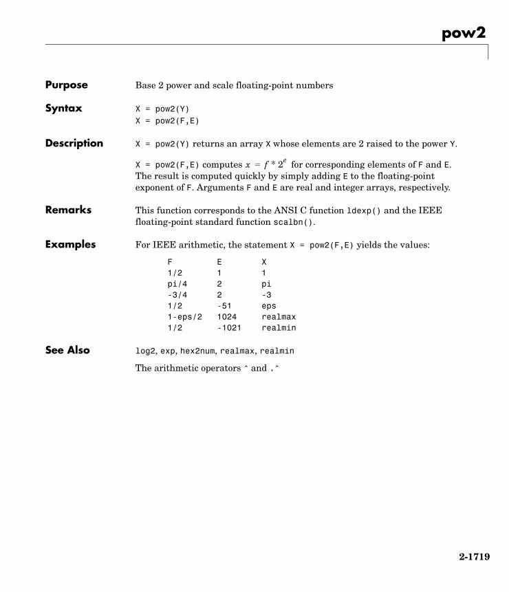
pow2
2-1719
2pow2Purpose Base 2 power and scale floating-point numbers
Syntax X = pow2(Y)X = pow2(F,E)
Description X = pow2(Y) returns an array X whose elements are 2 raised to the power Y.
X = pow2(F,E) computes for corresponding elements of F and E. The result is computed quickly by simply adding E to the floating-point exponent of F. Arguments F and E are real and integer arrays, respectively.
Remarks This function corresponds to the ANSI C function ldexp() and the IEEE floating-point standard function scalbn().
Examples For IEEE arithmetic, the statement X = pow2(F,E) yields the values:
F E X1/2 1 1pi/4 2 pi-3/4 2 -31/2 -51 eps1-eps/2 1024 realmax1/2 -1021 realmin
See Also log2, exp, hex2num, realmax, realmin
The arithmetic operators ^ and .^
x f * 2e=

ppval
2-1720
2ppvalPurpose Evaluate piecewise polynomial.
Syntax v = ppval(pp,xx)v = ppval(xx,pp)
Description v = ppval(pp,xx) returns the value at the points xx of the piecewise polynomial contained in pp, as constructed by spline or the spline utility mkpp.
v = ppval(xx,pp) returns the same result but can be used with functions like fminbnd, fzero and quad that take a function as an argument.
Examples Compare the results of integrating the function cos
a = 0; b = 10;int1 = quad(@cos,a,b,[],[])
int1 = -0.5440
with the results of integrating the piecewise polynomial pp that approximates the cosine function by interpolating the computed values x and y.
x = a:b; y = cos(x);pp = spline(x,y);int2 = quad(@ppval,a,b,[],[],pp)
int2 = -0.5485
int1 provides the integral of the cosine function over the interval [a,b], while int2 provides the integral over the same interval of the piecewise polynomial pp.
See Also mkpp, spline, unmkpp

prefdir
2-1721
2prefdirPurpose Return directory containing preferences, history, and layout files
Syntax prefdird = prefdird = prefdir(1)
Description prefdir returns the directory that contains preferences for MATLAB and related products (matlab.prf), the command history (history.m), the MATLAB shortcuts (shortcuts.xml), and the MATLAB desktop layout files (MATLABDesktop.xml and Your_Saved_LayoutMATLABLayout.xml).
On Macintosh platforms, the directory might be in a hidden folder, for example, myname/.matlab/R14. To access the directory, select Go -> Go to Folder in the Finder. In the resulting dialog box, type the path returned by prefdir and press Enter.
d = prefdir returns the name of the directory containing preferences and related files, but does not ensure its existence.
d = prefdir(1) creates a directory for preferences and related files if one does not exist.
Examples Run
prefdir
MATLAB returns
ans =
C:\WINNT\Profiles\tbear.MATHWORKS\Application Data\MathWorks\MATLAB\R14
Running dir for the directory shows
. history.m
.. matlab.prf cwdhistory.m MATLABDesktop.xmlshortcuts.xml
and possibly other files for other MathWorks products and any desktop layouts you saved.

prefdir
2-1722
See Also Fonts, Colors, and Other Preferences

preferences
2-1723
2preferencesPurpose Display Preferences dialog box for MATLAB and related products
Graphical Interface
As an alternative to the preferences function, select Preferences from the File menu in the MATLAB desktop or any desktop tool.
Syntax preferences
Description preferences displays the Preferences dialog box, from which you can make changes to options for MATLAB and related products. For more information, see Fonts, Colors, and Other Preferences.

primes
2-1724
2primesPurpose Generate list of prime numbers
Syntax p = primes(n)
Description p = primes(n) returns a row vector of the prime numbers less than or equal to n. A prime number is one that has no factors other than 1 and itself.
Examples p = primes(37)
p =
2 3 5 7 11 13 17 19 23 29 31 37
See Also factor

print, printopt
2-1725
2print, printoptPurpose Create hardcopy output
Syntax printprint filenameprint -ddriverprint -dformatprint -dformat filenameprint -smodelnameprint ... -options[pcmd,dev] = printopt
Description print and printopt produce hardcopy output. All arguments to the print command are optional. You can use them in any combination or order.
print sends the contents of the current figure, including bitmap representations of any user interface controls, to the printer using the device and system printing command defined by printopt.
print filename directs the output to the file designated by filename. If filename does not include an extension, print appends an appropriate extension.
print -ddriver prints the figure using the specified printer driver, (such as color PostScript). If you omit -ddriver, print uses the default value stored in printopt.m. The Printer Driver table lists all supported device types.
print -dformat copies the figure to the system clipboard (Windows only). A valid format for this operation is either -dmeta (Windows Enhanced Metafile) or -dbitmap (Windows Bitmap).
print -dformat filename exports the figure to the specified file using the specified graphics format, (such as TIFF). The Graphics Format table lists all supported graphics file formats.
print -smodelname prints the current Simulink model modelname.
print -options specifies print options that modify the action of the print command. (For example, the noui option suppresses printing of user interface controls.) The Options section lists available options.

print, printopt
2-1726
print(...) is the function form of print. It enables you to pass variables for any input arguments. This form is useful for passing filenames and handles. See Batch Processing for an example.
[pcmd,dev] = printopt returns strings containing the current system-dependent printing command and output device. printopt is an M-file used by print to produce the hardcopy output. You can edit the M-file printopt.m to set your default printer type and destination.
pcmd and dev are platform-dependent strings. pcmd contains the command that print uses to send a file to the printer. dev contains the printer driver or graphics format option for the print command. Their defaults are platform dependent.
Drivers The table below shows the complete list of printer drivers supported by MATLAB. If you do not specify a driver, MATLAB uses the default setting shown in the previous table.
Some of the drivers are available from a product called Ghostscript, which is shipped with MATLAB. The last column indicates when Ghostscript is used.
Some drivers are not available on all platforms. This is noted in the first column of the table.
Platform System Printing Command
Driver or Format
UNIX lpr r dps2
Windows COPY /B %s LPT1: dwin
Printer Driver PRINT Command Option String
GhostScript
Canon BubbleJet BJ10e -dbj10e Yes
Canon BubbleJet BJ200 color -dbj200 Yes
Canon Color BubbleJet BJC-70/BJC-600/BJC-4000 -dbjc600 Yes
Canon Color BubbleJet BJC-800 -dbjc800 Yes

print, printopt
2-1727
DEC LN03 -dln03 Yes
Epson and compatible 9- or 24-pin dot matrix print drivers
-depson Yes
Epson and compatible 9-pin with interleaved lines (triple resolution)
-deps9high Yes
Epson LQ-2550 and compatible; color (not supported on HP-700)
-depsonc Yes
Fujitsu 3400/2400/1200 -depsonc Yes
HP DesignJet 650C color (not supported on Windows) -ddnj650c Yes
HP DeskJet 500 -ddjet500 Yes
HP DeskJet 500C (creates black and white output) -dcdjmono Yes
HP DeskJet 500C (with 24 bit/pixel color and high-quality Floyd-Steinberg color dithering) (not supported on Windows)
-dcdjcolor Yes
HP DeskJet 500C/540C color (not supported on Windows)
-dcdj500 Yes
HP Deskjet 550C color (not supported on Windows) -dcdj550 Yes
HP DeskJet and DeskJet Plus -ddeskjet Yes
HP LaserJet -dlaserjet Yes
HP LaserJet+ -dljetplus Yes
HP LaserJet IIP -dljet2p Yes
HP LaserJet III -dljet3 Yes
HP LaserJet 4.5L and 5P -dljet4 Yes
HP LaserJet 5 and 6 -dpxlmono Yes
Printer Driver PRINT Command Option String
GhostScript

print, printopt
2-1728
Note Generally, Level 2 PostScript files are smaller and are rendered more quickly when printing than Level 1 PostScript files. However, not all PostScript printers support Level 2, so determine the capabilities of your printer before using those drivers. Level 2 PostScript is the default for UNIX. You can change this default by editing the printopt.m file.
Graphics Format Files
To save your figure as a graphics-format file, specify a format switch and filename. To set the resolution of the output file for a built-in MATLAB format, use the -r switch. (For example, -r300 sets the output resolution to 300 dots per inch.) The -r switch is also supported for Windows Enhanced Metafiles but is not supported for Ghostscript formats.
HP PaintJet color -dpaintjet Yes
HP PaintJet XL color -dpjxl Yes
HP PaintJet XL color -dpjetxl Yes
HP PaintJet XL300 color (not supported on Windows) -dpjxl300 Yes
HPGL for HP 7475A and other compatible plotters. (Renderer cannot be set to Z-buffer.)
-dhpgl No
IBM 9-pin Proprinter -dibmpro Yes
PostScript black and white -dps No
PostScript color -dpsc No
PostScript Level 2 black and white -dps2 No
PostScript Level 2 color -dpsc2 No
Windows color (Windows only) -dwinc No
Windows monochrome (Windows only) -dwin No
Printer Driver PRINT Command Option String
GhostScript

print, printopt
2-1729
The table below shows the supported output formats for exporting from MATLAB and the switch settings to use. In some cases, a format is available both as a MATLAB output filter and as a Ghostscript output filter. The first column indicates this by showing “MATLAB” or “Ghostscript” in parentheses. All formats except for EMF are supported on both the PC and UNIX platforms.
Graphics Format Bitmap or Vector
PRINT Command Option String
MATLAB or Ghostscript
BMP monochrome BMP Bitmap -dbmpmono Ghostscript
BMP 24-bit BMP Bitmap -dbmp16m Ghostscript
BMP 8-bit (256-color) BMP *this format uses a fixed colormap
Bitmap -dbmp256 Ghostscript
BMP 24-bit Bitmap -dbmp MATLAB
EMF Vector -dmeta MATLAB
EPS black and white Vector -deps MATLAB
EPS color Vector -depsc MATLAB
EPS Level 2 black and white Vector -deps2 MATLAB
EPS Level 2 color Vector -depsc2 MATLAB
HDF 24-bit Bitmap -dhdf MATLAB
ILL (Adobe Illustrator) Vector -dill MATLAB
JPEG 24-bit Bitmap -djpeg MATLAB
PBM (plain format) 1-bit Bitmap -dpbm Ghostscript
PBM (raw format) 1-bit Bitmap -dpbmraw Ghostscript
PCX 1-bit Bitmap -dpcxmono Ghostscript
PCX 24-bit color PCX file format, three 8-bit planes
Bitmap -dpcx24b Ghostscript

print, printopt
2-1730
The TIFF image format is supported on all platforms by almost all word processors for importing images. JPEG is a lossy, highly compressed format that is supported on all platforms for image processing and for inclusion into HTML documents on the World Wide Web. To create these formats, MATLAB renders the figure using the Z-buffer rendering method and the resulting bitmap is then saved to the specified file.
Options This table summarizes options that you can specify for print. The second column also shows which tutorial sections contain more detailed information.
PCX 8-bit Newer color PCX file format (256-color)
Bitmap -dpcx256 Ghostscript
PCX Older color PCX file format (EGA/VGA, 16-color)
Bitmap -dpcx16 Ghostscript
PCX 8-bit Bitmap -dpcx MATLAB
PDF Color PDF file format -dpdf Ghostscript
PGM Portable Graymap (plain format) Bitmap -dpgm Ghostscript
PGM Portable Graymap (raw format) Bitmap -dpgmraw Ghostscript
PNG 24-bit Bitmap -dpng MATLAB
PPM Portable Pixmap, plain format Bitmap -dppm Ghostscript
PPM Portable Pixmap raw format Bitmap -dppmraw Ghostscript
TIFF 24-bit Bitmap -dtiff or -dtiffn
MATLAB
TIFF preview for EPS Files Bitmap -tiff
Graphics Format Bitmap or Vector
PRINT Command Option String
MATLAB or Ghostscript

print, printopt
2-1731
The sections listed are located under Printing and Exporting Figures with MATLAB.
Option Description
-adobecset PostScript only. Use PostScript default character set encoding. See “Early PostScript 1 Printers.”
-append PostScript only. Append figure to existing PostScript file. See “Settings That Are Driver Specific.”
-cmyk PostScript only. Print with CMYK colors instead of RGB. See “Setting CMYK Color.”
-ddriver Printing only. Printer driver to use. See Drivers table.
-dformat Exporting only. Graphics format to use. See Graphics Format Files table.
-dsetup Display the Print Setup dialog.
-fhandle Handle of figure to print. Note that you cannot specify both this option and the -swindowtitle option. See “Which Figure Is Printed.”
-loose PostScript and Ghostscript only. Use loose bounding box for PostScript. See “Producing Uncropped Figures.”
-noui Suppress printing of user interface controls. See “Excluding User Interface Controls.”
-opengl Render using the OpenGL algorithm. Note that you cannot specify this method in conjunction with -zbuffer or -painters. See “Selecting a Renderer.”
-painters Render using the Painter’s algorithm. Note that you cannot specify this method in conjunction with -zbuffer or -opengl. See “Selecting a Renderer.”
-Pprinter Specify name of printer to use. See “Selecting Printer.”
-rnumber PostScript and Ghostscript only. Specify resolution in dots per inch. See “Setting the Resolution.”

print, printopt
2-1732
Paper Sizes MATLAB supports a number of standard paper sizes. You can select from the following list by setting the PaperType property of the figure or selecting a supported paper size from the Print dialog box.
-swindowtitle Specify name of Simulink system window to print. Note that you cannot specify both this option and the -fhandle option. See “Which Figure Is Printed.”
-v Windows only. Display the Windows Print dialog box. The v stands for “verbose mode.”
-zbuffer Render using the Z-buffer algorithm. Note that you cannot specify this method in conjunction with -opengl or -painters. See “Selecting a Renderer.”
Option Description
Property Value Size (Width-by-Height)
usletter 8.5-by-11 inches
uslegal 11-by-14 inches
tabloid 11-by-17 inches
A0 841-by-1189 mm
A1 594-by-841 mm
A2 420-by-594 mm
A3 297-by-420 mm
A4 210-by-297 mm
A5 148-by-210 mm
B0 1029-by-1456 mm
B1 728-by-1028 mm
B2 514-by-728 mm

print, printopt
2-1733
Printing Tips This section includes information about specific printing issues.
Figures with Resize FunctionsThe print command produces a warning when you print a figure having a callback routine defined for the figure ResizeFcn. To avoid the warning, set the figure PaperPositionMode property to auto or select Match Figure Screen Size in the File->Page Setup dialog box.
Troubleshooting MS-Windows PrintingIf you encounter problems such as segmentation violations, general protection faults, or application errors, or the output does not appear as you expect when using MS-Windows printer drivers, try the following:
B3 364-by-514 mm
B4 257-by-364 mm
B5 182-by-257 mm
arch-A 9-by-12 inches
arch-B 12-by-18 inches
arch-C 18-by-24 inches
arch-D 24-by-36 inches
arch-E 36-by-48 inches
A 8.5-by-11 inches
B 11-by-17 inches
C 17-by-22 inches
D 22-by-34 inches
E 34-by-43 inches
Property Value Size (Width-by-Height)

print, printopt
2-1734
• If your printer is PostScript compatible, print with one of the MATLAB built-in PostScript drivers. There are various PostScript device options that you can use with the print command: they all start with −dps.
• The behavior you are experiencing may occur only with certain versions of the print driver. Contact the print driver vendor for information on how to obtain and install a different driver.
• Try printing with one of the MATLAB built-in Ghostscript devices. These devices use Ghostscript to convert PostScript files into other formats, such as HP LaserJet, PCX, Canon BubbleJet, and so on.
• Copy the figure as a Windows Enhanced Metafile using the Edit-->Copy Figure menu item on the figure window menu or the print −dmeta option at the command line. You can then import the file into another application for printing.
You can set copy options in the figure’s File-->Preferences-->Copying Options dialog box. The Windows Enhanced Metafile clipboard format produces a better quality image than Windows Bitmap.
Printing MATLAB GUIsYou can generally obtain better results when printing a figure window that contains MATLAB uicontrols by setting these key properties:
• Set the figure PaperPositionMode property to auto. This ensures the printed version is the same size as the onscreen version. With PaperPositionMode set to auto MATLAB does not resize the figure to fit the current value of the PaperPosition. This is particularly important if you have specified a figure ResizeFcn, because if MATLAB resizes the figure during the print operation, the ResizeFcn is automatically called.
To set PaperPositionMode on the current figure, use the commandset(gcf,'PaperPositionMode','auto')
• Set the figure InvertHardcopy property to off. By default, MATLAB changes the figure background color of printed output to white, but does not change the color of uicontrols. If you have set the background color, for example, to match the gray of the GUI devices, you must set InvertHardcopy to off to preserve the color scheme.
To set InvertHardcopy on the current figure, use the commandset(gcf,'InvertHardcopy','off')

print, printopt
2-1735
• Use a color device if you want lines and text that are in color on the screen to be written to the output file as colored objects. Black and white devices convert colored lines and text to black or white to provide the best contrast with the background and to avoid dithering.
• Use the print command’s −loose option to prevent MATLAB from using a bounding box that is tightly wrapped around objects contained in the figure. This is important if you have intentionally used space between uicontrols or axes and the edge of the figure and you want to maintain this appearance in the printed output.
Notes on Printing Interpolated Shading with PostScript DriversMATLAB can print surface objects (such as graphs created with surf or mesh) using interpolated colors. However, only patch objects that are composed of triangular faces can be printed using interpolated shading.
Printed output is always interpolated in RGB space, not in the colormap colors. This means that if you are using indexed color and interpolated face coloring, the printed output can look different from what is displayed on screen.
PostScript files generated for interpolated shading contain the color information of the graphics object’s vertices and require the printer to perform the interpolation calculations. This can take an excessive amount of time and in some cases, printers may actually time out before finishing the print job. One solution to this problem is to interpolate the data and generate a greater number of faces, which can then be flat shaded.
To ensure that the printed output matches what you see on the screen, print using the -zbuffer option. To obtain higher resolution (for example, to make text look better), use the -r option to increase the resolution. There is, however, a tradeoff between the resolution and the size of the created PostScript file, which can be quite large at higher resolutions. The default resolution of 150 dpi generally produces good results. You can reduce the size of the output file by making the figure smaller before printing it and setting the figure PaperPositionMode to auto, or by just setting the PaperPosition property to a smaller size.
Examples Specifying the Figure to PrintYou can print a noncurrent figure by specifying the figure’s handle. If a figure has the title “Figure No. 2”, its handle is 2. The syntax is

print, printopt
2-1736
print -fhandle
This example prints the figure whose handle is 2, regardless of which figure is the current figure.
print -f2
Note You must use the -f option if the figure’s handle is hidden (i.e., its HandleVisibility property is set to off).
This example saves the figure with the handle -f2 to a PostScript file named Figure2, which can be printed later.
print -f2 -dps 'Figure2.ps'
If the figure uses noninteger handles, use the figure command to get its value, and then pass it in as the first argument.
h = figure('IntegerHandle','off')print h -depson
You can also pass a figure handle as a variable to the function form of print. For example,
h = figure; plot(1:4,5:8)print(h)
This example uses the function form of print to enable a filename to be passed in as a variable.
filename = 'mydata';print('-f3', '-dpsc', filename);
(Because a filename is specified, the figure will be printed to a file.)
Specifying the Model to PrintTo print a noncurrent Simulink model, use the -s option with the title of the window. For example, this command prints the Simulink window titled f14.
print -sf14

print, printopt
2-1737
If the window title includes any spaces, you must call the function form rather than the command form of print. For example, this command saves Simulink window title Thruster Control.
print('-sThruster Control')
To print the current system, use
print -s
For information about issues specific to printing Simulink windows, see the Simulink documentation.
This example prints a surface plot with interpolated shading. Setting the current figure’s (gcf) PaperPositionMode to auto enables you to resize the figure window and print it at the size you see on the screen. See Options and the previous section for information on the −zbuffer and −r200 options.
surf(peaks)shading interpset(gcf,'PaperPositionMode','auto')print −dpsc2 −zbuffer −r200
Batch ProcessingYou can use the function form of print to pass variables containing file names. For example, this for loop creates a series of graphs and prints each one with a different file name.
for k=1:length(fnames)surf(Z(:,:,k))print('-dtiff','-r200',fnames(k))
end
Tiff PreviewThe command
print -depsc -tiff -r300 picture1
saves the current figure at 300 dpi, in a color Encapsulated PostScript file named picture1.eps. The -tiff option creates a 72 dpi TIFF preview, which many word processor applications can display on screen after you import the EPS file. This enables you to view the picture on screen within your word

print, printopt
2-1738
processor and print the document to a PostScript printer using a resolution of 300 dpi.
See Also orient, figure

printdlg
2-1739
2printdlgPurpose Display print dialog box
Syntax printdlgprintdlg(fig)printdlg('-crossplatform',fig)printdlg('-setup',fig)
Description printdlg prints the current figure.
printdlg(fig) creates a dialog box from which you can print the figure window identified by the handle fig. Note that uimenus do not print.
printdlg('-crossplatform',fig) displays the standard cross-platform MATLAB printing dialog rather than the built-in printing dialog box for Microsoft Windows computers. Insert this option before the fig argument.
printdlg('-setup',fig) forces the printing dialog to appear in a setup mode. Here one can set the default printing options without actually printing.

printpreview
2-1740
2printpreviewPurpose
Preview figure to be printed
Syntax printpreviewprintpreview(f)
Description printpreview displays a dialog box showing the figure in the currently active figure window as it will be printed. The figure is displayed with a 1/4 size thumbnail or full size image.
printpreview(f) displays a dialog box showing the figure having the handle f as it will be printed.
You can select any of the following options from the Print Preview dialog box.
See Also printdlg, pagesetupdlg
Option Button Description
Print... Close Print Preview and open the Print dialog
Page Setup... Open the Page Setup dialog
Zoom In Display a full size image of the page
Zoom Out Display a 1/4 scaled image of the page
Close Close the Print Preview dialog

prod
2-1741
2prodPurpose Product of array elements
Syntax B = prod(A)B = prod(A,dim)
Description B = prod(A) returns the products along different dimensions of an array.
If A is a vector, prod(A) returns the product of the elements.
If A is a matrix, prod(A) treats the columns of A as vectors, returning a row vector of the products of each column.
If A is a multidimensional array, prod(A) treats the values along the first non-singleton dimension as vectors, returning an array of row vectors.
B = prod(A,dim) takes the products along the dimension of A specified by scalar dim.
Examples The magic square of order 3 is
M = magic(3)
M =8 1 63 5 74 9 2
The product of the elements in each column is
prod(M) =
96 45 84
The product of the elements in each row can be obtained by:
prod(M,2) =
4810572
See Also cumprod, diff, sum
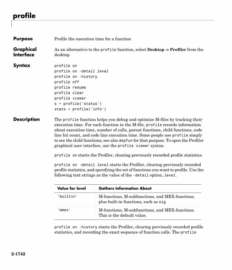
profile
2-1742
2profilePurpose Profile the execution time for a function
Graphical Interface
As an alternative to the profile function, select Desktop -> Profiler from the desktop.
Syntax profile onprofile on -detail levelprofile on -historyprofile offprofile resumeprofile clearprofile viewers = profile('status')stats = profile('info')
Description The profile function helps you debug and optimize M-files by tracking their execution time. For each function in the M-file, profile records information about execution time, number of calls, parent functions, child functions, code line hit count, and code line execution time. Some people use profile simply to see the child functions; see also depfun for that purpose. To open the Profiler graphical user interface, use the profile viewer syntax.
profile on starts the Profiler, clearing previously recorded profile statistics.
profile on -detail level starts the Profiler, clearing previously recorded profile statistics, and specifying the set of functions you want to profile. Use the following text strings as the value of the -detail option, level.
profile on -history starts the Profiler, clearing previously recorded profile statistics, and recording the exact sequence of function calls. The profile
Value for level Gathers Information About
'builtin' M-functions, M-subfunctions, and MEX-functions, plus built-in functions, such as eig
'mmex' M-functions, M-subfunctions, and MEX-functions. This is the default value.

profile
2-1743
function records up to 10,000 function entry and exit events. For more than 10,000 events, profile continues to record other profile statistics, but not the sequence of calls. By default, the history option is not enabled.
profile off stops the Profiler.
profile resume restarts the Profiler without clearing previously recorded statistics.
profile clear clears the statistics recorded by profile.
profile viewer stops the Profiler and displays the results in the Profiler window.
S = profile('status') returns a structure containing information about the current status of the Profiler. The table lists the fields in the order they appear in the structure.
stats = profile('info') stops the Profiler and displays a structure containing the results. Use this function to access the data generated by profile. The table lists the fields in the order they appear in the structure.
Field Values
ProfilerStatus 'on' or 'off'
DetailLevel 'mmex' or 'builtin'
HistoryTracking 'on' or 'off'
Field Description
FunctionTable Structure array containing statistics about each functions called
FunctionHistory Array containing function call history
ClockPrecision Precision of profile’s time measurement

profile
2-1744
The FunctionTable field is an array of structures, where each structure contains information about one of the functions or subfunctions called during execution. The following table lists these fields in the order they appear in the structure.
Name Name of the profiler
ClockSpeed Estimated clock speed of the CPU
Field Description
FunctionName Function name, includes subfunction references
FileName Filename is a fully qualified path
Type M-functions, MEX-functions, and many other types of functions including M-subfunctions, nested functions, and anonymous functions
NumCalls Number of times this function was called
TotalTime Total time spent in this function and its child functions
TotalRecursiveTime No longer used. Ignore value.
Children FunctionTable indices to child functions
Parents FunctionTable indices to parent functions
Field Description

profile
2-1745
Examples This example profiles the MATLAB magic command and then displays the results in the Profiler window. The example then retrieves the profile data on which the HTML display is based and uses the profsave command to save the profile data in HTML form.
profile onplot(magic(35))profile viewerp = profile('info');profsave(p,'profile_results')
Another way to save profile data is to store it in a MAT-file. This example stores the profile data in a MAT-file, clears the profile data from memory, and then loads the profile data from the MAT-file. This example also shows a way to bring the reloaded profile data into the Profiler graphical interface as live profile data; not as a static HTML page.
p = profile('info');save myprofiledata pclear pload myprofiledataprofview(0,p)
ExecutedLines Array containing line-by-line details for the function being profiled.Column 1: Number of the line that executed. If a line was not executed, it does not appear in this matrix. Column 2: Number of times that line was executedColumn 3: Total time spent on that line. Note: The sum of Column 3 does not necessarily add up to the function's TotalTime.
IsRecursive Boolean value: True if recursive, otherwise False
AcceleratorMessages No longer used
Field Description

profile
2-1746
This example illustrates an effective way to view the results of profiling when the history option is enabled. The history data describes the sequence of functions entered and exited during execution. The profile command returns history data in the FunctionHistory field of the structure it returns. The history data is a 2-by-n array. The first row contains Boolean values where 1 means entrance into a function and 0 means exit from a function. The second row identifies the function being entered or exited by its index in the FunctionTable field. This example reads the history data and displays it in the MATLAB Command Window.
profile on -historyplot(magic(4));p = profile('info');
for n = 1:size(p.FunctionHistory,2) if p.FunctionHistory(1,n)==0 str = 'entering function: '; else str = ' exiting function: '; end disp([str p.FunctionTable(p.FunctionHistory(2,n)).FunctionName]);end
See Also depdir, depfun, mlint, profsave
See Profiling for Improving Performance

profsave
2-1747
2profsavePurpose Save profile report in HTML format
Syntax profsaveprofsave(profinfo)profsave(profinfo,dirname)
Description profsave executes the profile('info') function and saves the results in HTML format. profsave creates a separate HTML file for each function listed in the FunctionTable field of the structure returned by profile. By default, profsave stores the HTML files in a subdirectory of the current directory named profile_results.
profsave(profinfo) saves the profiling results, profinfo, in HTML format. profinfo is a structure of profiling information returned by the profile('info') function.
profsave(profinfo,dirname) saves the profiling results, profinfo, in HTML format. profsave creates a separate HTML file for each function listed in the FunctionTable field of profinfo and stores them in the directory specified by dirname.
Examples Run profile and save the results.
profile onplot(magic(5))profile offprofsave(profile('info'),'myprofile_results')
See Also profile
Profiling for Improving Performance

propedit
2-1748
2propeditPurpose Starts the Property Editor
Syntax propeditpropedit(handle_list)propedit(handle_list,'v6')
Description propedit starts the Property Editor, a graphical user interface to the properties of graphics objects. There must be a current figure to call propedit without an object handle.
propedit(handle_list) edits the properties for the object (or objects) in handle_list.
propedit(handle_list,'v6') displays the MATLAB Version 6 Property Editor.
Starting the Property Editor enables plot editing mode for the figure.
Note The Version 6 Property Editor may not work with all objects.
See Also inspect, plotedit, propertyeditor

propertyeditor
2-1749
2propertyeditor
Purpose Show or hide property editor
Syntax propertyeditor('on')propertyeditor('off')propertyeditor('toggle'), propertyeditorpropertyeditor(figure_handle,...)
Description propertyeditor('on') displays the property editor on the current figure.
propertyeditor('off') hides the property editor on the current figure.
propertyeditor('toggle') or propertyeditor toggles the visibility of the property editor on the current figure.
propertyeditor(figure_handle,...) displays or hides the property editor on the figure specified by figure_handle.
See Also plotbrowser, figurepalette

psi
2-1750
2psiPurpose Psi (polygamma) function
Syntax Y = psi(X)Y = psi(k,X)Y = psi(k0:k1,X)
Description Y = psi(X) evaluates the function for each element of array X. X must be real and nonnegative. The function, also known as the digamma function, is the logarithmic derivative of the gamma function
Y = psi(k,X) evaluates the kth derivative of at the elements of X. psi(0,X) is the digamma function, psi(1,X) is the trigamma function, psi(2,X) is the tetragamma function, etc.
Y = psi(k0:k1,X) evaluates derivatives of order k0 through k1 at X. Y(k,j) is the (k-1+k0)th derivative of , evaluated at X(j).
Examples Example 1. Use the psi function to calculate Euler's constant, .
format long-psi(1)ans = 0.57721566490153
-psi(0,1)ans = 0.57721566490153
Example 2. The trigamma function of 2, psi(1,2), is the same as .
format longpsi(1,2)ans = 0.64493406684823
ψψ
ψ x( ) digamma x( )=d log Γ x( )( )( )
dx----------------------------------=
d Γ x( )( ) dx⁄Γ x( )
-----------------------------=
ψ
ψ
γ
π2 6⁄( ) 1–

psi
2-1751
pi^2/6 - 1ans = 0.64493406684823
Example 3. This code produces the first page of Table 6.1 in Abramowitz and Stegun [1].
x = (1:.005:1.250)'; [x gamma(x) gammaln(x) psi(0:1,x)' x-1]
Example 4. This code produces a portion of Table 6.2 in [1].
psi(2:3,1:.01:2)'
See Also gamma, gammainc, gammaln
References [1] Abramowitz, M. and I. A. Stegun, Handbook of Mathematical Functions, Dover Publlications, 1965, Sections 6.3 and 6.4.

publish
2-1752
2publishPurpose Run M-file containing cells, and save results to file of specified type
Graphical Interface
As an alternative to the publish function, use the File -> Publish To menu items in the Editor/Debugger.
Syntax publish('script')publish('script', 'format')publish('script', 'options')
Description publish('script') runs the file named script and publishes the code, comments, and results to an HTML output file. The output file is named script.html and is stored, along with other supporting output files, in an html subdirectory in script’s directory.
publish('script', 'format') runs the file named script and publishes the code, comments, and results to an output file using the specified format. Allowable values for format are html (the default), xml, tex for LaTeX, doc for Microsoft Word documents, and ppt for Microsoft PowerPoint documents. The output file is named script.format and is stored, along with other supporting output files, in an html subdirectory in script’s directory.
publish('script', 'options') provides a structure of options that may contain any of the following fields (first choice listed is the default):
Field Values
format 'html' | 'doc' | 'ppt' | 'xml' | 'rpt' | 'latex'
stylesheet '' | an XSL filename (ignored unless format is HTML or XML)
outputDir '' (an html subfolder below the file) | full path
imageFormat 'png' | any supported by PRINT or IMWRITE, depending on figureSnapMethod
figureSnapMethod 'print' | 'getframe'

publish
2-1753
Examples To publish the file d:/mymfiles/sine_wave.m to HTML, run
publish('d:/mymfiles/sine_wave.m', 'html')
MATLAB runs the file and saves the code, comments, and results to d:/mymfiles/html/sine_wave.html. Open that file in a browser to view the published document.
See Also notebook
Publishing to HTML, XML, LaTeX, Word and PowerPoint Using Cells
useNewFigure true | false
maxHeight [] | positive integer (pixels)
maxWidth [] | positive integer (pixels)
showCode true | false
evalCode true | false
stopOnError true | false
createThumbnail true | false
Field Values

pwd
2-1754
2pwdPurpose Display current directory
Graphical Interface
As an alternative to the pwd function, use the current directory field in the MATLAB desktop toolbar.
Syntax pwds = pwd
Description pwd displays the current working directory.
s = pwd returns the current directory to the variable s.
See Also cd, dir, fileparts, mfilename, path, what

qmr
2-1755
2qmrPurpose Quasi-Minimal Residual method
Syntax x = qmr(A,b)qmr(A,b,tol)qmr(A,b,tol,maxit)qmr(A,b,tol,maxit,M)qmr(A,b,tol,maxit,M1,M2)qmr(A,b,tol,maxit,M1,M2,x0)qmr(afun,b,tol,maxit,m1fun,m2fun,x0,p1,p2,...)[x,flag] = qmr(A,b,...)[x,flag,relres] = qmr(A,b,...)[x,flag,relres,iter] = qmr(A,b,...)[x,flag,relres,iter,resvec] = qmr(A,b,...)
Description x = qmr(A,b) attempts to solve the system of linear equations A*x=b for x. The n-by-n coefficient matrix A must be square and should be large and sparse. The column vector b must have length n. A can be a function afun such that afun(x) returns A*x and afun(x,'transp') returns A'*x.
If qmr converges, a message to that effect is displayed. If qmr fails to converge after the maximum number of iterations or halts for any reason, a warning message is printed displaying the relative residual norm(b-A*x)/norm(b) and the iteration number at which the method stopped or failed.
qmr(A,b,tol) specifies the tolerance of the method. If tol is [], then qmr uses the default, 1e-6.
qmr(A,b,tol,maxit) specifies the maximum number of iterations. If maxit is [], then qmr uses the default, min(n,20).
qmr(A,b,tol,maxit,M) and qmr(A,b,tol,maxit,M1,M2) use preconditioners M or M = M1*M2 and effectively solve the system inv(M)*A*x = inv(M)*b for x. If M is [] then qmr applies no preconditioner. M can be a function mfun such that mfun(x) returns M\x and mfun(x,'transp') returns M'\x.
qmr(A,b,tol,maxit,M1,M2,x0) specifies the initial guess. If x0 is [], then qmr uses the default, an all zero vector.

qmr
2-1756
qmr(afun,b,tol,maxit,m1fun,m2fun,x0,p1,p2,...) passes parameters p1,p2,... to functions afun(x,p1,p2,...) and afun(x,p1,p2,...,'transp') and similarly to the preconditioner functions m1fun and m2fun.
[x,flag] = qmr(A,b,...) also returns a convergence flag.
Whenever flag is not 0, the solution x returned is that with minimal norm residual computed over all the iterations. No messages are displayed if the flag output is specified.
[x,flag,relres] = qmr(A,b,...) also returns the relative residual norm(b-A*x)/norm(b). If flag is 0, relres <= tol.
[x,flag,relres,iter] = qmr(A,b,...) also returns the iteration number at which x was computed, where 0 <= iter <= maxit.
[x,flag,relres,iter,resvec] = qmr(A,b,...) also returns a vector of the residual norms at each iteration, including norm(b-A*x0).
Examples Example 1.
n = 100;on = ones(n,1);A = spdiags([-2*on 4*on -on],-1:1,n,n);b = sum(A,2);
Flag Convergence
0 qmr converged to the desired tolerance tol within maxit iterations.
1 qmr iterated maxit times but did not converge.
2 Preconditioner M was ill-conditioned.
3 The method stagnated. (Two consecutive iterates were the same.)
4 One of the scalar quantities calculated during qmr became too small or too large to continue computing.

qmr
2-1757
tol = 1e-8; maxit = 15;M1 = spdiags([on/(-2) on],-1:0,n,n);M2 = spdiags([4*on -on],0:1,n,n);x = qmr(A,b,tol,maxit,M1,M2,[]);
Alternatively, use this matrix-vector product function
function y = afun(x,n,transp_flag)if (nargin > 2) & strcmp(transp_flag,'transp') y = 4 * x; y(1:n-1) = y(1:n-1) - 2 * x(2:n); y(2:n) = y(2:n) - x(1:n-1);else y = 4 * x; y(2:n) = y(2:n) - 2 * x(1:n-1); y(1:n-1) = y(1:n-1) - x(2:n);end
as input to qmr
x1 = qmr(@afun,b,tol,maxit,M1,M2,[],n);
Example 2.
load west0479;A = west0479;b = sum(A,2);[x,flag] = qmr(A,b)
flag is 1 because qmr does not converge to the default tolerance 1e-6 within the default 20 iterations.
[L1,U1] = luinc(A,1e-5);[x1,flag1] = qmr(A,b,1e-6,20,L1,U1)
flag1 is 2 because the upper triangular U1 has a zero on its diagonal, and qmr fails in the first iteration when it tries to solve a system such as U1*y = r for y using backslash.
[L2,U2] = luinc(A,1e-6);[x2,flag2,relres2,iter2,resvec2] = qmr(A,b,1e-15,10,L2,U2)
flag2 is 0 because qmr converges to the tolerance of 1.6571e-016 (the value of relres2) at the eighth iteration (the value of iter2) when preconditioned by

qmr
2-1758
the incomplete LU factorization with a drop tolerance of 1e-6. resvec2(1) = norm(b) and resvec2(9) = norm(b-A*x2). You can follow the progress of qmr by plotting the relative residuals at each iteration starting from the initial estimate (iterate number 0).
semilogy(0:iter2,resvec2/norm(b),'-o')xlabel('iteration number')ylabel('relative residual')
See Also bicg, bicgstab, cgs, gmres, lsqr, luinc, minres, pcg, symmlq
@ (function handle), \ (backslash)
References [1] Barrett, R., M. Berry, T. F. Chan, et al., Templates for the Solution of Linear Systems: Building Blocks for Iterative Methods, SIAM, Philadelphia, 1994.
[2] Freund, Roland W. and Nöel M. Nachtigal, “QMR: A quasi-minimal residual method for non-Hermitian linear systems”, SIAM Journal: Numer. Math. 60, 1991, pp. 315-339.
0 1 2 3 4 5 6 7 810
−16
10−14
10−12
10−10
10−8
10−6
10−4
10−2
100
102
iteration number
rela
tive
resi
dual
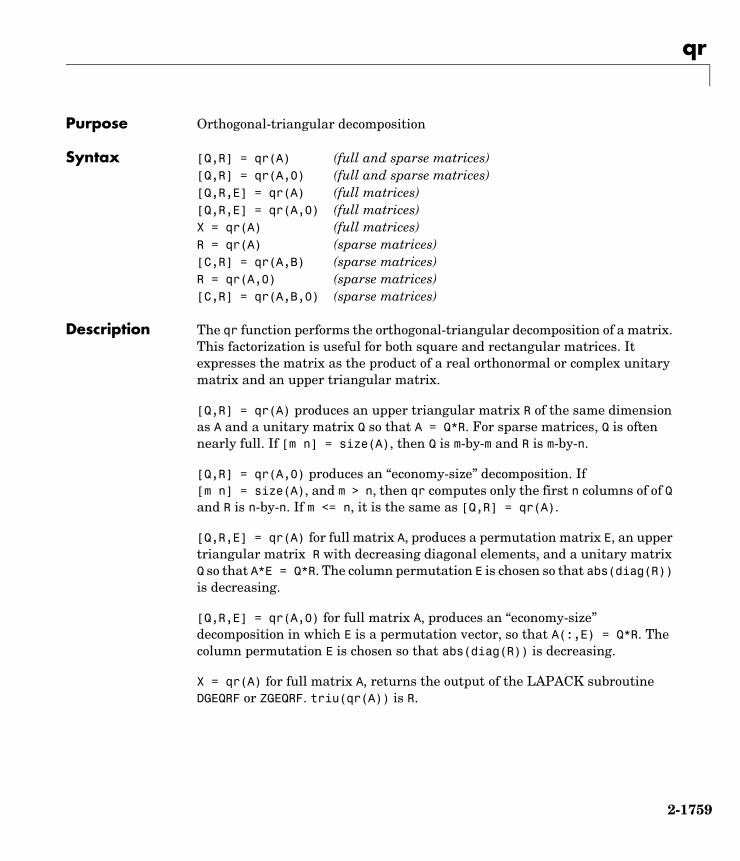
qr
2-1759
2qrPurpose Orthogonal-triangular decomposition
Syntax [Q,R] = qr(A) (full and sparse matrices)[Q,R] = qr(A,0) (full and sparse matrices)[Q,R,E] = qr(A) (full matrices)[Q,R,E] = qr(A,0) (full matrices)X = qr(A) (full matrices)R = qr(A) (sparse matrices)[C,R] = qr(A,B) (sparse matrices)R = qr(A,0) (sparse matrices)[C,R] = qr(A,B,0) (sparse matrices)
Description The qr function performs the orthogonal-triangular decomposition of a matrix. This factorization is useful for both square and rectangular matrices. It expresses the matrix as the product of a real orthonormal or complex unitary matrix and an upper triangular matrix.
[Q,R] = qr(A) produces an upper triangular matrix R of the same dimension as A and a unitary matrix Q so that A = Q*R. For sparse matrices, Q is often nearly full. If [m n] = size(A), then Q is m-by-m and R is m-by-n.
[Q,R] = qr(A,0) produces an “economy-size” decomposition. If [m n] = size(A), and m > n, then qr computes only the first n columns of of Q and R is n-by-n. If m <= n, it is the same as [Q,R] = qr(A).
[Q,R,E] = qr(A) for full matrix A, produces a permutation matrix E, an upper triangular matrix R with decreasing diagonal elements, and a unitary matrix Q so that A*E = Q*R. The column permutation E is chosen so that abs(diag(R)) is decreasing.
[Q,R,E] = qr(A,0) for full matrix A, produces an “economy-size” decomposition in which E is a permutation vector, so that A(:,E) = Q*R. The column permutation E is chosen so that abs(diag(R)) is decreasing.
X = qr(A) for full matrix A, returns the output of the LAPACK subroutine DGEQRF or ZGEQRF. triu(qr(A)) is R.

qr
2-1760
R = qr(A) for sparse matrix A, produces only an upper triangular matrix, R. The matrix R provides a Cholesky factorization for the matrix associated with the normal equations,
R'*R = A'*A
This approach avoids the loss of numerical information inherent in the computation of A'*A. It may be preferred to [Q,R] = qr(A) since Q is always nearly full.
[C,R] = qr(A,B) for sparse matrix A, applies the orthogonal transformations to B, producing C = Q'*B without computing Q. B and A must have the same number of rows.
R = qr(A,0) and [C,R] = qr(A,B,0) for sparse matrix A, produce “economy-size” results.
For sparse matrices, the Q-less QR factorization allows the solution of sparse least squares problems
with two steps
[C,R] = qr(A,b)x = R\c
If A is sparse but not square, MATLAB uses the two steps above for the linear equation solving backslash operator, i.e., x = A\b.
Examples Example 1. Start with
A = [ 1 2 3 4 5 6 7 8 9 10 11 12 ]
This is a rank-deficient matrix; the middle column is the average of the other two columns. The rank deficiency is revealed by the factorization:
[Q,R] = qr(A)
Q =
minimize Ax b–

qr
2-1761
-0.0776 -0.8331 0.5444 0.0605-0.3105 -0.4512 -0.7709 0.3251-0.5433 -0.0694 -0.0913 -0.8317-0.7762 0.3124 0.3178 0.4461
R =
-12.8841 -14.5916 -16.29920 -1.0413 -2.08260 0 0.00000 0 0
The triangular structure of R gives it zeros below the diagonal; the zero on the diagonal in R(3,3) implies that R, and consequently A, does not have full rank.
Example 2. This examples uses matrix A from the first example. The QR factorization is used to solve linear systems with more equations than unknowns. For example, let
b = [1;3;5;7]
The linear system represents four equations in only three unknowns. The best solution in a least squares sense is computed by
x = A\b
which produces
Warning: Rank deficient, rank = 2, tol = 1.4594E-014x =
0.50000
0.1667
The quantity tol is a tolerance used to decide if a diagonal element of R is negligible. If [Q,R,E] = qr(A), then
tol = max(size(A))*eps*abs(R(1,1))
The solution x was computed using the factorization and the two steps
y = Q'*b;x = R\y
Ax b=

qr
2-1762
The computed solution can be checked by forming . This equals to within roundoff error, which indicates that even though the simultaneous equations
are overdetermined and rank deficient, they happen to be consistent. There are infinitely many solution vectors x; the QR factorization has found just one of them.
Algorithm The qr function uses LAPACK routines to compute the QR decomposition:
See Also lu, null, orth, qrdelete, qrinsert, qrupdate
The arithmetic operators \ and /
References [1] Anderson, E., Z. Bai, C. Bischof, S. Blackford, J. Demmel, J. Dongarra, J. Du Croz, A. Greenbaum, S. Hammarling, A. McKenney, and D. Sorensen, LAPACK User’s Guide (http://www.netlib.org/lapack/lug/lapack_lug.html), Third Edition, SIAM, Philadelphia, 1999.
Ax b
Ax b=
Syntax Real Complex
R = qr(A)R = qr(A,0)
DGEQRF ZGEQRF
[Q,R] = qr(A)[Q,R] = qr(A,0)
DGEQRF, DORGQR ZGEQRF, ZUNGQR
[Q,R,e] = qr(A)[Q,R,e] = qr(A,0)
DGEQP3, DORGQR ZGEQPF, ZUNGQR

qrdelete
2-1763
2qrdeletePurpose Delete column or row from QR factorization
Syntax [Q1,R1] = qrdelete(Q,R,j)[Q1,R1] = qrdelete(Q,R,j,'col')[Q1,R1] = qrdelete(Q,R,j,'row')
Description [Q1,R1] = qrdelete(Q,R,j) returns the QR factorization of the matrix A1, where A1 is A with the column A(:,j) removed and [Q,R] = qr(A) is the QR factorization of A.
[Q1,R1] = qrdelete(Q,R,j,'col') is the same as qrdelete(Q,R,j).
[Q1,R1] = qrdelete(Q,R,j,'row') returns the QR factorization of the matrix A1, where A1 is A with the row A(j,:) removed and [Q,R] = qr(A) is the QR factorization of A.
Examples A = magic(5);[Q,R] = qr(A);j = 3;[Q1,R1] = qrdelete(Q,R,j,'row');
Q1 = 0.5274 -0.5197 -0.6697 -0.0578 0.7135 0.6911 0.0158 0.1142 0.3102 -0.1982 0.4675 -0.8037 0.3413 -0.4616 0.5768 0.5811
R1 = 32.2335 26.0908 19.9482 21.4063 23.3297 0 -19.7045 -10.9891 0.4318 -1.4873 0 0 22.7444 5.8357 -3.1977 0 0 0 -14.5784 3.7796
returns a valid QR factorization, although possibly different from
A2 = A; A2(j,:) = [];[Q2,R2] = qr(A2)

qrdelete
2-1764
Q2 = -0.5274 0.5197 0.6697 -0.0578 -0.7135 -0.6911 -0.0158 0.1142 -0.3102 0.1982 -0.4675 -0.8037 -0.3413 0.4616 -0.5768 0.5811
R2 = -32.2335 -26.0908 -19.9482 -21.4063 -23.3297 0 19.7045 10.9891 -0.4318 1.4873 0 0 -22.7444 -5.8357 3.1977 0 0 0 -14.5784 3.7796
Algorithm The qrdelete function uses a series of Givens rotations to zero out the appropriate elements of the factorization.
See Also planerot, qr, qrinsert

qrinsert
2-1765
2qrinsertPurpose Insert column or row into QR factorization
Syntax [Q1,R1] = qrinsert(Q,R,j,x)[Q1,R1] = qrinsert(Q,R,j,x,'col')[Q1,R1] = qrinsert(Q,R,j,x,'row')
Description [Q1,R1] = qrinsert(Q,R,j,x) returns the QR factorization of the matrix A1, where A1 is A = Q*R with the column x inserted before A(:,j). If A has n columns and j = n+1, then x is inserted after the last column of A.
[Q1,R1] = qrinsert(Q,R,j,x,'col') is the same as qrinsert(Q,R,j,x).
[Q1,R1] = qrinsert(Q,R,j,x,'row') returns the QR factorization of the matrix A1, where A1 is A = Q*R with an extra row, x, inserted before A(j,:).
Examples A = magic(5); [Q,R] = qr(A);j = 3; x = 1:5;[Q1,R1] = qrinsert(Q,R,j,x,'row')
Q1 = 0.5231 0.5039 -0.6750 0.1205 0.0411 0.0225 0.7078 -0.6966 0.0190 -0.0788 0.0833 -0.0150 0.0308 0.0592 0.0656 0.1169 0.1527 -0.9769 0.1231 0.1363 0.3542 0.6222 0.6398 0.2104 0.3077 0.1902 0.4100 0.4161 -0.7264 -0.0150 0.3385 0.4500 0.4961 -0.6366 0.1761 0.0225
R1 = 32.4962 26.6801 21.4795 23.8182 26.0031 0 19.9292 12.4403 2.1340 4.3271 0 0 24.4514 11.8132 3.9931 0 0 0 20.2382 10.3392 0 0 0 0 16.1948 0 0 0 0 0
returns a valid QR factorization, although possibly different from

qrinsert
2-1766
A2 = [A(1:j-1,:); x; A(j:end,:)];[Q2,R2] = qr(A2)
Q2 = -0.5231 0.5039 0.6750 -0.1205 0.0411 0.0225 -0.7078 -0.6966 -0.0190 0.0788 0.0833 -0.0150 -0.0308 0.0592 -0.0656 -0.1169 0.1527 -0.9769 -0.1231 0.1363 -0.3542 -0.6222 0.6398 0.2104 -0.3077 0.1902 -0.4100 -0.4161 -0.7264 -0.0150 -0.3385 0.4500 -0.4961 0.6366 0.1761 0.0225
R2 = -32.4962 -26.6801 -21.4795 -23.8182 -26.0031 0 19.9292 12.4403 2.1340 4.3271 0 0 -24.4514 -11.8132 -3.9931 0 0 0 -20.2382 -10.3392 0 0 0 0 16.1948 0 0 0 0 0
Algorithm The qrinsert function inserts the values of x into the jth column (row) of R. It then uses a series of Givens rotations to zero out the nonzero elements of R on and below the diagonal in the jth column (row).
See Also planerot, qr, qrdelete

qrupdate
2-1767
2qrupdateDescription Rank 1 update to QR factorization
Syntax [Q1,R1] = qrupdate(Q,R,u,v)
Description [Q1,R1] = qrupdate(Q,R,u,v) when [Q,R] = qr(A) is the original QR factorization of A, returns the QR factorization of A + u*v', where u and v are column vectors of appropriate lengths.
Remarks qrupdate works only for full matrices.
Examples The matrix
mu = sqrt(eps)
mu =
1.4901e-08
A = [ones(1,4); mu*eye(4)];
is a well-known example in least squares that indicates the dangers of forming A'*A. Instead, we work with the QR factorization – orthonormal Q and upper triangular R.
[Q,R] = qr(A);
As we expect, R is upper triangular.
R =
-1.0000 -1.0000 -1.0000 -1.0000 0 0.0000 0.0000 0.0000 0 0 0.0000 0.0000 0 0 0 0.0000 0 0 0 0
In this case, the upper triangular entries of R, excluding the first row, are on the order of sqrt(eps).
Consider the update vectors
u = [-1 0 0 0 0]'; v = ones(4,1);
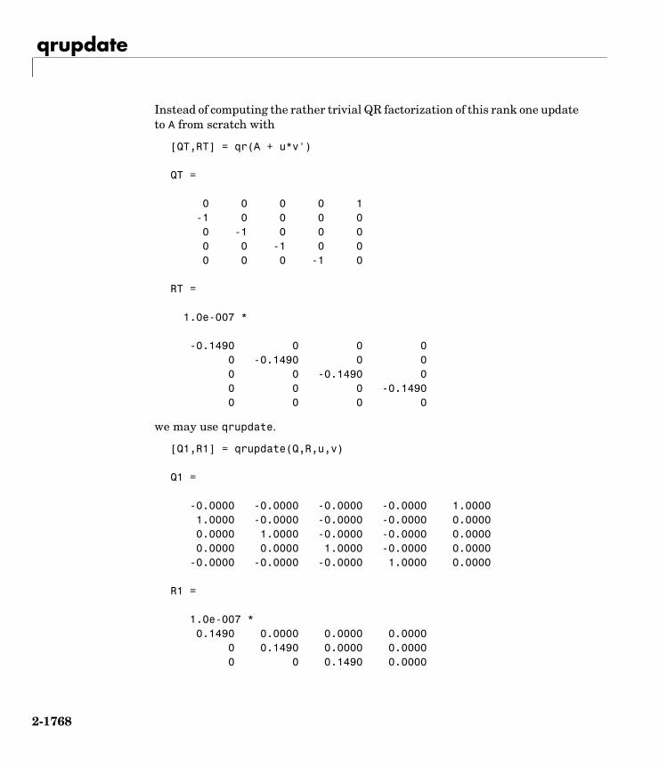
qrupdate
2-1768
Instead of computing the rather trivial QR factorization of this rank one update to A from scratch with
[QT,RT] = qr(A + u*v')
QT =
0 0 0 0 1 -1 0 0 0 0 0 -1 0 0 0 0 0 -1 0 0 0 0 0 -1 0
RT =
1.0e-007 *
-0.1490 0 0 0 0 -0.1490 0 0 0 0 -0.1490 0 0 0 0 -0.1490 0 0 0 0
we may use qrupdate.
[Q1,R1] = qrupdate(Q,R,u,v)
Q1 =
-0.0000 -0.0000 -0.0000 -0.0000 1.0000 1.0000 -0.0000 -0.0000 -0.0000 0.0000 0.0000 1.0000 -0.0000 -0.0000 0.0000 0.0000 0.0000 1.0000 -0.0000 0.0000 -0.0000 -0.0000 -0.0000 1.0000 0.0000
R1 =
1.0e-007 * 0.1490 0.0000 0.0000 0.0000 0 0.1490 0.0000 0.0000 0 0 0.1490 0.0000

qrupdate
2-1769
0 0 0 0.1490 0 0 0 0
Note that both factorizations are correct, even though they are different.
Algorithm qrupdate uses the algorithm in section 12.5.1 of the third edition of Matrix Computations by Golub and van Loan. qrupdate is useful since, if we take N = max(m,n), then computing the new QR factorization from scratch is roughly an algorithm, while simply updating the existing factors in this way is an algorithm.
References [1] Golub, Gene H. and Charles Van Loan, Matrix Computations, Third Edition, Johns Hopkins University Press, Baltimore, 1996
See Also cholupdate, qr
O N3( )O N2( )

quad, quad8
2-1770
2quad, quad8Purpose Numerically evaluate integral, adaptive Simpson quadrature
Note The quad8 function, which implemented a higher order method, is obsolete. The quadl function is its recommended replacement.
Syntax q = quad(fun,a,b)q = quad(fun,a,b,tol)q = quad(fun,a,b,tol,trace)[q,fcnt] = quadl(fun,a,b,...)
Description Quadrature is a numerical method used to find the area under the graph of a function, that is, to compute a definite integral.
q = quad(fun,a,b) tries to approximate the integral of function fun from a to b to within an error of 1e-6 using recursive adaptive Simpson quadrature. fun is a function handle for either an M-file function or an anonymous function. The function y = fun(x) should accept a vector argument x and return a vector result y, the integrand evaluated at each element of x.
Parameterizing Functions Called by Function Functions, in the online MATLAB documentation, explains how to provide addition parameters to the function fun, if necessary.
q = quad(fun,a,b,tol) uses an absolute error tolerance tol instead of the default which is 1.0e-6. Larger values of tol result in fewer function evaluations and faster computation, but less accurate results. In MATLAB version 5.3 and earlier, the quad function used a less reliable algorithm and a default relative tolerance of 1.0e-3.
q = quad(fun,a,b,tol,trace) with non-zero trace shows the values of [fcnt a b-a Q] during the recursion.
[q,fcnt] = quad(...) returns the number of function evaluations.
q f x( ) xda
b
∫=

quad, quad8
2-1771
The function quadl may be more efficient with high accuracies and smooth integrands.
Examples Pass M-file function handle @myfun to quad:
Q = quad(@myfun,0,2);
where the M-file myfun.m is
function y = myfun(x) y = 1./(x.^3-2*x-5);
Pass anonymous function handle F to quad:
F = @(x)1./(x.^3-2*x-5);Q = quad(F,0,2);
Algorithm quad implements a low order method using an adaptive recursive Simpson’s rule.
Diagnostics quad may issue one of the following warnings:
'Minimum step size reached' indicates that the recursive interval subdivision has produced a subinterval whose length is on the order of roundoff error in the length of the original interval. A nonintegrable singularity is possible.
'Maximum function count exceeded' indicates that the integrand has been evaluated more than 10,000 times. A nonintegrable singularity is likely.
'Infinite or Not-a-Number function value encountered' indicates a floating point overflow or division by zero during the evaluation of the integrand in the interior of the interval.
See Also dblquad, quadl, triplequad, @ (function handle), anonymous functions
References [1] Gander, W. and W. Gautschi, “Adaptive Quadrature – Revisited”, BIT, Vol. 40, 2000, pp. 84-101. This document is also available at http://www.inf.ethz.ch/personal/gander.

quadl
2-1772
2quadlPurpose Numerically evaluate integral, adaptive Lobatto quadrature
Syntax q = quadl(fun,a,b)q = quadl(fun,a,b,tol)q = quadl(fun,a,b,tol,trace)[q,fcnt] = quadl(fun,a,b,...)
Description q = quadl(fun,a,b) approximates the integral of function fun from a to b, to within an error of 10-6 using recursive adaptive Lobatto quadrature. fun is a function handle for either an M-file function or an anonymous function. fun accepts a vector x and returns a vector y, the function fun evaluated at each element of x.
Parameterizing Functions Called by Function Functions, in the online MATLAB documentation, explains how to provide addition parameters to the function fun, if necessary.
q = quadl(fun,a,b,tol) uses an absolute error tolerance of tol instead of the default, which is 1.0e-6. Larger values of tol result in fewer function evaluations and faster computation, but less accurate results.
quadl(fun,a,b,tol,trace) with non-zero trace shows the values of [fcnt a b-a q] during the recursion.
[q,fcnt] = quadl(...) returns the number of function evaluations.
Use array operators .*, ./ and .^ in the definition of fun so that it can be evaluated with a vector argument.
The function quad may be more efficient with low accuracies or nonsmooth integrands.
Examples Pass M-file function handle @myfun to quadl:
Q = quadl(@myfun,0,2);
where the M-file myfun.m is
function y = myfun(x) y = 1./(x.^3-2*x-5);
Pass anonymous function handle F to quadl:

quadl
2-1773
F = @(x) 1./(x.^3-2*x-5);Q = quadl(F,0,2);
Algorithm quadl implements a high order method using an adaptive Gauss/Lobatto qudrature rule.
Diagnostics quadl may issue one of the following warnings:
'Minimum step size reached' indicates that the recursive interval subdivision has produced a subinterval whose length is on the order of roundoff error in the length of the original interval. A nonintegrable singularity is possible.
'Maximum function count exceeded' indicates that the integrand has been evaluated more than 10,000 times. A nonintegrable singularity is likely.
'Infinite or Not-a-Number function value encountered' indicates a floating point overflow or division by zero during the evaluation of the integrand in the interior of the interval.
See Also dblquad, quad, triplequad, @ (function handle), anonymous functions
References [1] Gander, W. and W. Gautschi, “Adaptive Quadrature – Revisited”, BIT, Vol. 40, 2000, pp. 84-101. This document is also available at http://www.inf.ethz.ch/personal/gander.
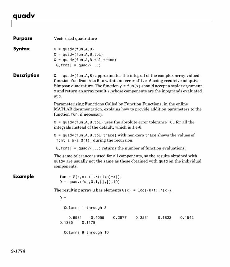
quadv
2-1774
2quadvPurpose Vectorized quadrature
Syntax Q = quadv(fun,A,B)Q = quadv(fun,A,B,tol)Q = quadv(fun,A,B,tol,trace)[Q,fcnt] = quadv(...)
Description Q = quadv(fun,A,B) approximates the integral of the complex array-valued function fun from A to B to within an error of 1.e-6 using recursive adaptive Simpson quadrature. The function y = fun(x) should accept a scalar argument x and return an array result Y, whose components are the integrands evaluated at x.
Parameterizing Functions Called by Function Functions, in the online MATLAB documentation, explains how to provide addition parameters to the function fun, if necessary.
Q = quadv(fun,A,B,tol) uses the absolute error tolerance TOL for all the integrals instead of the default, which is 1.e-6.
Q = quadv(fun,A,B,tol,trace) with non-zero trace shows the values of [fcnt a b-a Q(1)] during the recursion.
[Q,fcnt] = quadv(...) returns the number of function evaluations.
The same tolerance is used for all components, so the results obtained with quadv are usually not the same as those obtained with quad on the individual components.
Example fun = @(x,n) (1./((1:n)+x));Q = quadv(fun,0,1,[],[],10)
The resulting array Q has elements Q(k) = log((k+1)./(k)).
Q =
Columns 1 through 8
0.6931 0.4055 0.2877 0.2231 0.1823 0.1542 0.1335 0.1178
Columns 9 through 10

quadv
2-1775
0.1054 0.0953
See Also quad, dblquad, triplequad

questdlg
2-1776
2questdlgPurpose Create and display question dialog box
Syntax button = questdlg('qstring')button = questdlg('qstring','title')button = questdlg('qstring','title','default')button = questdlg('qstring','title','str1','str2','default')button = questdlg('qstring','title','str1','str2','str3','default')
Description button = questdlg('qstring') displays a modal dialog presenting the question 'qstring'. The dialog has three default buttons, Yes, No, and Cancel. If the user presses one of these three buttons, button is set to the name of the button pressed. If the user presses the close button on the dialog, button is set to the empty string. If the user presses the Return key, button is set to 'Yes'. 'qstring' is a cell array or a string that automatically wraps to fit within the dialog box.
button = questdlg('qstring','title') displays a question dialog with 'title' displayed in the dialog’s title bar.
button = questdlg('qstring','title','default') specifies which push button is the default in the event that the Return key is pressed. 'default' must be 'Yes', 'No', or 'Cancel'.
button = questdlg('qstring','title','str1','str2','default')creates a question dialog box with two push buttons labeled 'str1' and 'str2'. 'default' specifies the default button selection and must be 'str1' or 'str2'.
button = questdlg('qstring','title','str1','str2','str3','default') creates a question dialog box with three push buttons labeled 'str1', 'str2', and 'str3'. 'default' specifies the default button selection and must be 'str1', 'str2', or 'str3'.
In all cases where 'default' is specified, if'default' is not set to one of the button names, pressing the Return key displays a warning and the dialog remains open.
See Also inputdlg, textwrap

quit
2-1777
2quitPurpose Terminate MATLAB
Graphical Interface
As an alternative to the quit function, use the close box or select Exit MATLAB from the File menu in the MATLAB desktop.
Syntax quitquit cancelquit force
Description quit terminates MATLAB after running finish.m, if finish.m exists. The workspace is not automatically saved by quit. To save the workspace or perform other actions when quitting, create a finish.m file to perform those actions. For example, you can display a dialog box to confirm quitting using a finish.m file—see the following examples for details. If an error occurs while finish.m is running, quit is canceled so that you can correct your finish.m file without losing your workspace.
quit cancel is for use in finish.m and cancels quitting. It has no effect anywhere else.
quit force bypasses finish.m and terminates MATLAB. Use this to override finish.m, for example, if an errant finish.m will not let you quit.
Remarks When using Handle Graphics in finish.m, use uiwait, waitfor, or drawnow so that figures are visible. See the reference pages for these functions for more information.

quit
2-1778
Examples Two sample finish.m files are included with MATLAB. Use them to help you create your own finish.m, or rename one of the files to finish.m to use it.
• finishsav.m—Saves the workspace to a MAT-file when MATLAB quits.
• finishdlg.m—Displays a dialog allowing you to cancel quitting; it uses quit cancel and contains the following code:
button = questdlg('Ready to quit?', ... 'Exit Dialog','Yes','No','No');switch button case 'Yes', disp('Exiting MATLAB'); %Save variables to matlab.mat save case 'No', quit cancel;end
See Also finish, save, startup
quiverPurpose Quiver or velocity plot
Syntax quiver(x,y,u,v)quiver(u,v)quiver(...,scale)quiver(...,LineSpec)quiver(...,LineSpec,'filled')quiver(axes_handle,...)h = quiver(...)hlines = quiver('v6',...)
Description A quiver plot displays velocity vectors as arrows with components (u,v) at the points (x,y).
For example, the first vector is defined by components u(1),v(1) and is displayed at the point x(1),y(1).
quiver(x,y,u,v) plots vectors as arrows at the coordinates specified in each corresponding pair of elements in x and y. The matrices x, y, u, and v must all

quit
2-1779
be the same size and contain corresponding position and velocity components. However, x and y can also be vectors, as explained in the next section.
Expanding x and y CoordinatesMATLAB expands x and y if they are not matrices. This expansion is equivalent to calling meshgrid to generate matrices from vectors:
[x,y] = meshgrid(x,y);quiver(x,y,u,v)
In this case, the following must be true:
length(x) = n and length(y) = m, where [m,n] = size(u) = size(v).
The vector x corresponds to the columns of u and v, and vector y corresponds to the rows of u and v.
quiver(u,v) draws vectors specified by u and v at equally spaced points in the x-y plane.
quiver(...,scale) automatically scales the arrows to fit within the grid and then stretches them by the factor scale. scale = 2 doubles their relative length and scale = 0.5 halves the length. Use scale = 0 to plot the velocity vectors without automatic scaling.
quiver(...,LineSpec) specifies line style, marker symbol, and color using any valid LineSpec. quiver draws the markers at the origin of the vectors.
quiver(...,LineSpec,'filled') fills markers specified by LineSpec.
quiver(axes_handles,...) plots into the axes with handle axes_handle instead of the current axes (gca).
h = quiver(...) returns the handle to the quivergroup object.
Backward Compatible Version
hlines = quiver('v6',...) returns the handles of line objects instead of quivergroup objects for compatibility with MATLAB 6.5 and earlier.

quit
2-1780
Examples Showing the Gradient with Quiver PlotsPlot the gradient field of the function :
[X,Y] = meshgrid(-2:.2:2);Z = X.*exp(-X.^2 - Y.^2);[DX,DY] = gradient(Z,.2,.2);contour(X,Y,Z)hold onquiver(X,Y,DX,DY)colormap hsvhold off
See Also contour, LineSpec, plot, quiver3
“Direction and Velocity Plots” for related functions
Two-Dimensional Quiver Plots for more examples
See “Quivergroup Properties” for property descriptions
z xe x2 y2––( )=
−2 −1.5 −1 −0.5 0 0.5 1 1.5 2−2
−1.5
−1
−0.5
0
0.5
1
1.5
2

quiver3
2-1781
2quiver3Purpose Three-dimensional velocity plot
Syntax quiver3(x,y,z,u,v,w)quiver3(z,u,v,w)quiver3(...,scale)quiver3(...,LineSpec)quiver3(...,LineSpec,'filled')quiver3(axes_handle,...)h = quiver3(...)
Description A three-dimensional quiver plot displays vectors with components (u,v,w) at the points (x,y,z).
quiver3(x,y,z,u,v,w) plots vectors with components (u,v,w) at the points (x,y,z). The matrices x,y,z,u,v,w must all be the same size and contain the corresponding position and vector components.
quiver3(z,u,v,w) plots the vectors at the equally spaced surface points specified by matrix z. quiver3 automatically scales the vectors based on the distance between them to prevent them from overlapping.
quiver3(...,scale) automatically scales the vectors to prevent them from overlapping, then multiplies them by scale. scale = 2 doubles their relative length and scale = 0.5 halves them. Use scale = 0 to plot the vectors without the automatic scaling.
quiver3(...,LineSpec) specifies line type and color using any valid LineSpec.
quiver3(...,LineSpec,'filled') fills markers specified by LineSpec.
quiver3(axes_handles,...) plots into the axes with handle axes_handle instead of the current axes (gca).
h = quiver3(...) returns a vector of line handles.
Examples Plot the surface normals of the function .
[X,Y] = meshgrid(-2:0.25:2,-1:0.2:1);Z = X.* exp(-X.^2 - Y.^2);
z xe x2 y2––( )=

quiver3
2-1782
[U,V,W] = surfnorm(X,Y,Z);quiver3(X,Y,Z,U,V,W,0.5);hold onsurf(X,Y,Z);colormap hsvview(-35,45)axis ([-2 2 -1 1 -.6 .6])hold off
See Also axis, contour, LineSpec, plot, plot3, quiver, surfnorm, view
“Direction and Velocity Plots” for related functions
Three-Dimensional Quiver Plots for more examples
−2
−1
0
1
2
−1
−0.5
0
0.5
1
−0.4
−0.2
0
0.2
0.4
0.6

Quivergroup Properties
2-1783
2Quivergroup PropertiesModifying Properties
You can set and query graphics object properties using the set and get commands or the Property Editor (propertyeditor).
Note that you cannot define default properties for areaseries objects.
See Plot Objects for more information on quivergroup objects.
Quivergroup Property Descriptions
This section provides a description of properties. Curly braces enclose default values.
AutoScale on | off
Autoscale arrow length. Based on average spacing in the x and y directions, AutoScale scales the arrow length to fit within the grid-defined coordinate data and keeps the arrows from overlapping. After autoscaling, quiver applies the AutoScaleFactor to the arrow length.
AutoScaleFactor scalar (default = 0.9)
User-specified scale factor. When AutoScale is on, the quiver function applies this user-specified autoscale factor to the arrow length. A value of 2 doubles the length of the arrows; 0.5 halves the length.
BeingDeleted on | off Read Only
This object is being deleted. The BeingDeleted property provides a mechanism that you can use to determine if objects are in the process of being deleted. MATLAB sets the BeingDeleted property to on when the object’s delete function callback is called (see the DeleteFcn property). It remains set to on while the delete function executes, after which the object no longer exists.
For example, an object’s delete function might call other functions that act on a number of different objects. These functions might not need to perform actions on objects that are going to be deleted, and therefore can check the object’s BeingDeleted property before acting.
BusyAction cancel | queue
Callback routine interruption. The BusyAction property enables you to control how MATLAB handles events that potentially interrupt executing callbacks. If there is a callback function executing, callbacks invoked subsequently always attempt to interrupt it.
If the Interruptible property of the object whose callback is executing is set to on (the default), then interruption occurs at the next point where the event

Quivergroup Properties
2-1784
queue is processed. If the Interruptible property is off, the BusyAction property (of the object owning the executing callback) determines how MATLAB handles the event. The choices are
• cancel — Discard the event that attempted to execute a second callback routine.
• queue — Queue the event that attempted to execute a second callback routine until the current callback finishes.
ButtonDownFcn string or function handle
Button press callback function. A callback that executes whenever you press a mouse button while the pointer is over the quivergroup object.
This property can be
• A string that is a valid MATLAB expression
• The name of an M-file
• A function handle
The expression executes in the MATLAB workspace.
See Function Handle Callbacks for information on how to use function handles to define the callbacks.
Children array of graphics object handles
Children of the quivergroup object. An array containing the handles of all line objects parented to the quivergroup object (whether visible or not).
Note that if a child object’s HandleVisibility property is set to callback or off, its handle does not show up in the quiver Children property unless you set the Root ShowHiddenHandles property to on:
set(0,'ShowHiddenHandles','on')
Clipping on | off
Clipping mode. MATLAB clips quiver plots to the axes plot box by default. If you set Clipping to off, arrows might be displayed outside the axes plot box.
Color ColorSpec
Color of arrows. A three-element RGB vector or one of the MATLAB predefined names, specifying the arrow color. See the ColorSpec reference page for more

Quivergroup Properties
2-1785
information on specifying color. For example, the following statement shows the arrow color set to blue.
h = quiver(u,v,'Color','b');
CreateFcn string or function handle
Callback routine executed during object creation. This property defines a callback that executes when MATLAB creates a quivergroup object. You must specify the callback during the creation of the object. For example,
quiver(u,v,'CreateFcn',@CallbackFcn)
where @CallbackFcn is a function handle that references the callback function.
MATLAB executes this routine after setting all other quivergroup properties. Setting this property on an existing quivergroup object has no effect.
The handle of the object whose CreateFcn is being executed is accessible only through the root CallbackObject property, which you can query using gcbo.
See Function Handle Callbacks for information on how to use function handles to define the callback function.
DeleteFcn string or function handle
Callback executed during object deletion. A callback that executes when the quivergroup object is deleted (e.g., this might happen when you issue a delete command on the quivergroup object, its parent axes, or the figure containing it). MATLAB executes the callback before destroying the object’s properties so that the callback routine can query these values.
The handle of the object whose DeleteFcn is being executed is accessible only through the Root CallbackObject property, which can be queried using gcbo.
See Function Handle Callbacks for information on how to use function handles to define the callback function.
See the BeingDeleted property for related information.
DisplayName string
Label used by plot legends. The legend and the plot browser use this text for labels for any quivergroup objects appearing in these legends.

Quivergroup Properties
2-1786
EraseMode normal | none | xor | background
Erase mode. This property controls the technique MATLAB uses to draw and erase quiver child objects (the lines used to construct the arrows). Alternative erase modes are useful for creating animated sequences, where control of the way individual objects are redrawn is necessary to improve performance and obtain the desired effect.
• normal — Redraw the affected region of the display, performing the three-dimensional analysis necessary to ensure that all objects are rendered correctly. This mode produces the most accurate picture, but is the slowest. The other modes are faster but do not perform a complete redraw and are therefore less accurate.
• none — Do not erase objects when they are moved or destroyed. While the objects are still visible on the screen after erasing with EraseMode none, you cannot print these objects because MATLAB stores no information about their former locations.
• xor— Draw and erase the object by performing an exclusive OR (XOR) with each pixel index of the screen behind it. Erasing the object does not damage the color of the objects behind it. However, the color of the erased object depends on the color of the screen behind it and it is correctly colored only when it is over the axes background color (or the figure background color if the axes Color property is set to none). That is, it isn’t erased correctly if there are objects behind it.
• background — Erase the graphics objects by redrawing them in the axes background color, (or the figure background color if the axes Color property is set to none). This damages other graphics objects that are behind the erased object, but the erased object is always properly colored.
Printing with Nonnormal Erase ModesMATLAB always prints figures as if the EraseMode of all objects is normal. This means graphics objects created with EraseMode set to none, xor, or background can look different on screen than on paper. On screen, MATLAB might mathematically combine layers of colors (e.g., performing an XOR operation on a pixel color and the pixel behind it) and ignore three-dimensional sorting to obtain greater rendering speed. However, these techniques are not applied to the printed output.

Quivergroup Properties
2-1787
Set the axes background color with the axes Color property. Set the figure background color with the figure Color property.
You can use the MATLAB getframe command or other screen capture applications to create an image of a figure containing nonnormal mode objects.
HandleVisibility on | callback | off
Control access to object’s handle by command-line users and GUIs. This property determines when an object’s handle is visible in its parent’s list of children. HandleVisibility is useful for preventing command-line users from accidentally accessing the quivergroup object.
• on — Handles are always visible when HandleVisibility is on.
• callback — Setting HandleVisibility to callback causes handles to be visible from within callback routines or functions invoked by callback routines, but not from within functions invoked from the command line. This provides a means to protect GUIs from command-line users, while allowing callback routines to have access to object handles.
• off — Setting HandleVisibility to off makes handles invisible at all times. This might be necessary when a callback invokes a function that might potentially damage the GUI (such as evaluating a user-typed string) and so temporarily hides its own handles during the execution of that function.
Functions Affected by Handle VisibilityWhen a handle is not visible in its parent’s list of children, it cannot be returned by functions that obtain handles by searching the object hierarchy or querying handle properties. This includes get, findobj, gca, gcf, gco, newplot, cla, clf, and close.
Properties Affected by Handle VisibilityWhen a handle’s visibility is restricted using callback or off, the object’s handle does not appear in its parent’s Children property, figures do not appear in the root’s CurrentFigure property, objects do not appear in the root’s CallbackObject property or in the figure’s CurrentObject property, and axes do not appear in their parent’s CurrentAxes property.

Quivergroup Properties
2-1788
Overriding Handle VisibilityYou can set the root ShowHiddenHandles property to on to make all handles visible regardless of their HandleVisibility settings (this does not affect the values of the HandleVisibility properties). See also findall.
Handle ValidityHandles that are hidden are still valid. If you know an object’s handle, you can set and get its properties and pass it to any function that operates on handles.
HitTest on | off
Selectable by mouse click. HitTest determines whether the quivergroup object can become the current object (as returned by the gco command and the figure CurrentObject property) as a result of a mouse click on the line objects that compose the quiver plot. If HitTest is off, clicking the quivergroup object selects the object below it (which is usually the axes containing it).
HitTestArea on | off
Select quivergroup object on arrows or extent of graph. This property enables you to select quivergroup objects in two ways:
• Select by clicking quiver arrows (default).
• Select by clicking anywhere in the extent of the quiver plot.
When HitTestArea is off, you must click the quiver lines (excluding the base line) to select the quivergroup object. When HitTestArea is on, you can select the quivergroup object by clicking anywhere within the extent of the graph (i.e., anywhere within a rectangle that encloses all the arrows).
Interruptible on | off
Callback routine interruption mode. The Interruptible property controls whether a quivergroup object callback can be interrupted by subsequently invoked callbacks.
Only callbacks defined for the ButtonDownFcn property are affected by the Interruptible property. MATLAB checks for events that can interrupt a callback only when it encounters a drawnow, figure, getframe, or pause command in the routine. See the BusyAction property for related information.
Setting Interruptible to on allows any graphics object’s callback to interrupt callback routines originating from a quiver property. Note that MATLAB does

Quivergroup Properties
2-1789
not save the state of variables or the display (e.g., the handle returned by the gca or gcf command) when an interruption occurs.
LineStyle − | −− | : | −. | none
Line style. This property specifies the line style used for the quiver arrows. Available line styles are shown in the following table.
You can use LineStyle none when you want to place a marker at each point but do not want the points connected with a line (see the Marker property).
LineWidth scalar
Width of the quiver arrows. Specify this value in points (1 point = 1/72 inch). The default LineWidth is 0.5 points.
Marker character (see table)
Marker symbol. The Marker property specifies the type of markers that are displayed at the x- and y-coordinates. You can set values for the Marker property independently from the LineStyle property. Supported markers include those shown in the following table.
Symbol Line Style
− Solid line (default)
−− Dashed line
: Dotted line
−. Dash-dot line
none No line
Marker Specifier Description
+ Plus sign
o Circle
* Asterisk
. Point

Quivergroup Properties
2-1790
MarkerEdgeColor ColorSpec | none | auto
Marker edge color. The color of the marker or the edge color for filled markers (circle, square, diamond, pentagram, hexagram, and the four triangles). ColorSpec defines the color to use. none specifies no color, which makes nonfilled markers invisible. auto sets MarkerEdgeColor to the same color as the quiver Color property.
MarkerFaceColor ColorSpec | none | auto
Marker face color. The fill color for markers that are closed shapes (circle, square, diamond, pentagram, hexagram, and the four triangles). ColorSpec defines the color to use. none makes the interior of the marker transparent, allowing the background to show through. auto sets the fill color to the axes color, or to the figure color, if the axes Color property is set to none (which is the factory default for axes).
MarkerSize size in points
Marker size. A scalar specifying the size of the marker in points. The default value for MarkerSize is 6 points (1 point = 1/72 inch). Note that MATLAB draws the point marker (specified by the '.' symbol) at one-third the specified size.
x Cross
s Square
d Diamond
^ Upward-pointing triangle
v Downward-pointing triangle
> Right-pointing triangle
< Left-pointing triangle
p Five-pointed star (pentagram)
h Six-pointed star (hexagram)
none No marker (default)
Marker Specifier Description

Quivergroup Properties
2-1791
MaxHeadSize scalar (default = 0.2
Maximum size of arrowhead. A value determining the maximum size of the arrowhead relative to the length of the arrow.
Parent axes handle
Parent of quivergroup object. This property contains the handle of the quivergroup object’s parent object. The parent of a quivergroup object is the axes, hggroup, or hgtransform object that contains it.
See Objects That Can Contain Other Objects for more information on parenting graphics objects.
Selected on | off
Is object selected? When you set this property to on, MATLAB displays selection handles at the corners and midpoints if the SelectionHighlight property is also on (the default). You can, for example, define the ButtonDownFcn callback to set this property to on, thereby indicating that the quivergroup object is selected.
SelectionHighlight on | off
Objects are highlighted when selected. When the Selected property is on, MATLAB indicates the selected state by drawing selection handles on the arrows. When SelectionHighlight is off, MATLAB does not draw the handles.
ShowArrowHead on | off
Display arrowheads on vectors. When this property is on, MATLAB draws arrowheads on the vectors displayed by quiver. When you set this property to off, quiver draws the vectors as lines without arrowheads.
Tag string
User-specified object label. The Tag property provides a means to identify graphics objects with a user-specified label. This is particularly useful when you are constructing interactive graphics programs that would otherwise need to define object handles as global variables or pass them as arguments between callbacks.
For example, you might create a quivergroup object and set the Tag property:
t = quiver(u,v,'Tag','quiver1')

Quivergroup Properties
2-1792
When you want to access the quivergroup object, you can use findobj to find the object’s handle. The following statement changes the Color property of the object whose Tag is quiver1.
set(findobj('Tag','quiver1'),'Color','red')
Type string (read only)
Type of graphics object. This property contains a string that identifies the class of the graphics object. For stem objects, Type is 'hggroup'. This statement finds all the hggroup objects in the current axes.
t = findobj(gca,'Type','hggroup');
UIContextMenu handle of a uicontextmenu object
Associate a context menu with the quivergroup object. Assign this property the handle of a uicontextmenu object created in the quivergroup object’s parent figure. Use the uicontextmenu function to create the context menu. MATLAB displays the context menu whenever you right-click over the extent of the quivergroup object.
UserData array
User-specified data. This property can be any data you want to associate with the quivergroup object (including cell arrays and structures). The quivergroup object does not set values for this property, but you can access it using the set and get functions.
Visible on | off
Visibility of quivergroup object and its children. By default, stem object visibility is on. This means all children of the quivergroup object are visible unless the child object’s Visible property is set to off. Setting a quivergroup object’s Visible property to off also makes its children invisible.
UData matrix
One dimension of 2-D or 3-D vector components. UData, VData, and WData, together specify the components of the vectors displayed as arrows in the quiver graph. For example, the first vector is defined by components UData(1),VData(1),WData(1).
Quivergroup Properties
2-1793
UDataSource string (MATLAB variable)
Link UData to MATLAB variable. Set this property to a MATLAB variable that, by default, is evaluated in the base workspace to generate the UData.
MATLAB reevaluates this property only when you set it. Therefore, a change to workspace variables appearing in an expression does not change UData.
You can use the refreshdata function to force an update of the object’s data. refreshdata also enables you to specify that the data source variable be evaluated in the workspace of a function from which you call refreshdata.
See the refreshdata reference page for more information.
Note If you change one data source property to return data of a different dimension, you might cause the function to generate a warning and not render the graph until you have changed all data source properties to appropriate values.
VData matrix
One dimension of 2-D or 3-D vector components. UData, VData and WData (for 3-D) together specify the components of the vectors displayed as arrows in the quiver graph. For example, the first vector is defined by components UData(1),VData(1),WData(1).
VDataSource string (MATLAB variable)
Link VData to MATLAB variable. Set this property to a MATLAB variable that, by default, is evaluated in the base workspace to generate the VData.
MATLAB reevaluates this property only when you set it. Therefore, a change to workspace variables appearing in an expression does not change VData.
You can use the refreshdata function to force an update of the object’s data. refreshdata also enables you to specify that the data source variable be evaluated in the workspace of a function from which you call refreshdata.
See the refreshdata reference page for more information.

Quivergroup Properties
2-1794
Note If you change one data source property to return data of a different dimension, you might cause the function to generate a warning and not render the graph until you have changed all data source properties to appropriate values.
WData matrix
One dimension of 2-D or 3-D vector components. UData, VData and WData (for 3-D) together specify the components of the vectors displayed as arrows in the quiver graph. For example, the first vector is defined by components UData(1),VData(1),WData(1).
WDataSource string (MATLAB variable)
Link WData to MATLAB variable. Set this property to a MATLAB variable that, by default, is evaluated in the base workspace to generate the WData.
MATLAB reevaluates this property only when you set it. Therefore, a change to workspace variables appearing in an expression does not change WData.
You can use the refreshdata function to force an update of the object’s data. refreshdata also enables you to specify that the data source variable be evaluated in the workspace of a function from which you call refreshdata.
See the refreshdata reference page for more information.
Note If you change one data source property to return data of a different dimension, you might cause the function to generate a warning and not render the graph until you have changed all data source properties to appropriate values.
XData vector or matrix
X-axis coordinates of arrows. The quiver function draws an individual arrow at each x-axis location in the XData array. XData can be either a matrix equal in size to all other data properties or for 2-D, a vector equal in length to the number of columns in UData or VData. That is, length(XData) == size(UData,2).

Quivergroup Properties
2-1795
If you do not specify XData (i.e., the input argument X), the quiver function uses the indices of UData to create the quiver graph. See the XDataMode property for related information.
XDataMode auto | manual
Use automatic or user-specified x-axis values. If you specify XData (by setting the XData property or specifying the input argument X), the quiver function sets this property to manual.
If you set XDataMode to auto after having specified XData, the quiver function resets the x tick-mark labels to the indices of the U, V, and W data, overwriting any previous values.
XDataSource string (MATLAB variable)
Link XData to MATLAB variable. Set this property to a MATLAB variable that, by default, is evaluated in the base workspace to generate the XData.
MATLAB reevaluates this property only when you set it. Therefore, a change to workspace variables appearing in an expression does not change XData.
You can use the refreshdata function to force an update of the object’s data. refreshdata also enables you to specify that the data source variable be evaluated in the workspace of a function from which you call refreshdata.
See the refreshdata reference page for more information.
Note If you change one data source property to return data of a different dimension, you might cause the function to generate a warning and not render the graph until you have changed all data source properties to appropriate values.
YData vector or matrix
Y-axis coordinates of arrows. The quiver function draws an individual arrow at each y-axis location in the YData array. YData can be either a matrix equal in size to all other data properties or for 2-D, a vector equal in length to the number of rows in UData or VData. That is, length(YData) == size(UData,1).

Quivergroup Properties
2-1796
If you do not specify YData (i.e., the input argument Y), the quiver function uses the indices of VData to create the quiver graph. See the YDataMode property for related information.
The input argument y in the quiver function calling syntax assigns values to YData.
YDataMode auto | manual
Use automatic or user-specified y-axis values. If you specify YData (by setting the YData property or specifying the input argument Y), MATLAB sets this property to manual.
If you set YDataMode to auto after having specified YData, MATLAB resets the y tick-mark labels to the indices of the U, V, and W data, overwriting any previous values.
YDataSource string (MATLAB variable)
Link YData to MATLAB variable. Set this property to a MATLAB variable that, by default, is evaluated in the base workspace to generate the YData.
MATLAB reevaluates this property only when you set it. Therefore, a change to workspace variables appearing in an expression does not change YData.
You can use the refreshdata function to force an update of the object’s data. refreshdata also enables you to specify that the data source variable be evaluated in the workspace of a function from which you call refreshdata.
See the refreshdata reference page for more information.
Note If you change one data source property to a variable that contains data of a different dimension, you might cause the function to generate a warning and not render the graph until you have changed all data source properties to appropriate values.
ZData vector or matrix
Z-axis coordinates of arrows. The quiver function draws an individual arrow at each z-axis location in the ZData array. ZData must be a matrix equal in size to XData and YData.

Quivergroup Properties
2-1797
The input argument z in the quiver3 function calling syntax assigns values to ZData.

qz
2-1798
2qzPurpose QZ factorization for generalized eigenvalues
Syntax [AA,BB,Q,Z,] = qz(A,B)[AA,BB,Q,Z,V,W] = qz(A,B)qz(A,B,flag)
Description The qz function gives access to intermediate results in the computation of generalized eigenvalues.
[AA,BB,Q,Z] = qz(A,B) for square matrices A and B, produces upper quasitriangular matrices AA and BB, and unitary matrices Q and Z such that Q*A*Z = AA, and Q*B*Z = BB. For complex matrices, AA and BB are triangular.
[AA,BB,Q,Z,V,W] = qz(A,B) also produces matrices V and W whose columns are generalized eigenvectors.
qz(A,B,flag) for real matrices A and B, produces one of two decompositions depending on the value of flag:
If AA is triangular, the diagonal elements of AA and BB, and , are the generalized eigenvalues that satisfy
The eigenvalues produced by
are the ratios of the s and s.
If AA is triangular, the diagonal elements of AA and BB,
'complex' Produces a possibly complex decomposition with a triangular AA. For compatibility with earlier versions, 'complex' is the default.
'real' Produces a real decomposition with a quasitriangular AA, containing 1-by-1 and 2-by-2 blocks on its diagonal.
α diag AA( )=β diag BB( )=
A*V*β B*V*α=β*W '*A α*W '*B=
λ eig A B,( )=
α β
λ α . /β=

rand
2-1799
2randPurpose Uniformly distributed random numbers and arrays
Syntax Y = rand(n)Y = rand(m,n)Y = rand([m n])Y = rand(m,n,p,...)Y = rand([m n p...])Y = rand(size(A))rands = rand('state')
Description The rand function generates arrays of random numbers whose elements are uniformly distributed in the interval (0,1).
Y = rand(n) returns an n-by-n matrix of random entries. An error message appears if n is not a scalar.
Y = rand(m,n) or Y = rand([m n]) returns an m-by-n matrix of random entries.
Y = rand(m,n,p,...) or Y = rand([m n p...]) generates random arrays.
Y = rand(size(A)) returns an array of random entries that is the same size as A.
rand, by itself, returns a scalar whose value changes each time it’s referenced.
s = rand('state') returns a 35-element vector containing the current state of the uniform generator. To change the state of the generator:
rand('state',s) Resets the state to s.
rand('state',0) Resets the generator to its initial state.
rand('state',j) For integer j, resets the generator to its j-th state.
rand('state',sum(100*clock)) Resets it to a different state each time.

rand
2-1800
Examples Example 1. R = rand(3,4) may produce
R = 0.2190 0.6793 0.5194 0.0535 0.0470 0.9347 0.8310 0.5297 0.6789 0.3835 0.0346 0.6711
This code makes a random choice between two equally probable alternatives.
if rand < .5 'heads' else 'tails' end
Example 2. Generate a uniform distribution of random numbers on a specified interval [a,b]. To do this, multiply the output of rand by (b-a) then add a. For example, to generate a 5-by-5 array of uniformly distributed random numbers on the interval [10,50]
a = 10; b = 50;x = a + (b-a) * rand(5)x =
18.1106 10.6110 26.7460 43.5247 30.1125 17.9489 39.8714 43.8489 10.7856 38.3789 34.1517 27.8039 31.0061 37.2511 27.1557 20.8875 47.2726 18.1059 25.1792 22.1847 17.9526 28.6398 36.8855 43.2718 17.5861
See Also randn, randperm, sprand, sprandn

randn
2-1801
2randnPurpose Normally distributed random numbers and arrays
Syntax Y = randn(n)Y = randn(m,n)Y = randn([m n])Y = randn(m,n,p,...)Y = randn([m n p...])Y = randn(size(A))randns = randn('state')
Description The randn function generates arrays of random numbers whose elements are normally distributed with mean 0, variance , and standard deviation
.
Y = randn(n) returns an n-by-n matrix of random entries. An error message appears if n is not a scalar.
Y = randn(m,n) or Y = randn([m n]) returns an m-by-n matrix of random entries.
Y = randn(m,n,p,...) or Y = randn([m n p...]) generates random arrays.
Y = randn(size(A)) returns an array of random entries that is the same size as A.
randn, by itself, returns a scalar whose value changes each time it’s referenced.
s = randn('state') returns a 2-element vector containing the current state of the normal generator. To change the state of the generator:
randn('state',s) Resets the state to s.
randn('state',0) Resets the generator to its initial state.
randn('state',j) For integer j, resets the generator to its jth state.
randn('state',sum(100*clock)) Resets it to a different state each time.
σ2 1=σ 1=
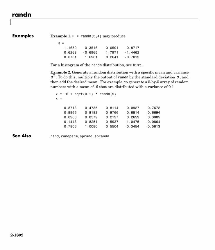
randn
2-1802
Examples Example 1. R = randn(3,4) may produce
R = 1.1650 0.3516 0.0591 0.8717 0.6268 -0.6965 1.7971 -1.4462 0.0751 1.6961 0.2641 -0.7012
For a histogram of the randn distribution, see hist.
Example 2. Generate a random distribution with a specific mean and variance . To do this, multiply the output of randn by the standard deviation , and
then add the desired mean. For example, to generate a 5-by-5 array of random numbers with a mean of .6 that are distributed with a variance of 0.1
x = .6 + sqrt(0.1) * randn(5)x =
0.8713 0.4735 0.8114 0.0927 0.7672 0.9966 0.8182 0.9766 0.6814 0.6694 0.0960 0.8579 0.2197 0.2659 0.3085 0.1443 0.8251 0.5937 1.0475 -0.0864 0.7806 1.0080 0.5504 0.3454 0.5813
See Also rand, randperm, sprand, sprandn
σ2 σ
randperm
2-1803
2randpermPurpose Random permutation
Syntax p = randperm(n)
Description p = randperm(n) returns a random permutation of the integers 1:n.
Remarks The randperm function calls rand and therefore changes rand’s state.
Examples randperm(6) might be the vector
[3 2 6 4 1 5]
or it might be some other permutation of 1:6.
See Also permute

rank
2-1804
2rankPurpose Rank of a matrix
Syntax k = rank(A)k = rank(A,tol)
Description The rank function provides an estimate of the number of linearly independent rows or columns of a full matrix.
k = rank(A) returns the number of singular values of A that are larger than the default tolerance, max(size(A))*norm(A)*eps.
k = rank(A,tol) returns the number of singular values of A that are larger than tol.
Remark Use sprank to determine the structural rank of a sparse matrix.
Algorithm There are a number of ways to compute the rank of a matrix. MATLAB uses the method based on the singular value decomposition, or SVD. The SVD algorithm is the most time consuming, but also the most reliable.
The rank algorithm is
s = svd(A);tol = max(size(A))*s(1)*eps;r = sum(s > tol);
See Also sprank
References [1] Anderson, E., Z. Bai, C. Bischof, S. Blackford, J. Demmel, J. Dongarra, J. Du Croz, A. Greenbaum, S. Hammarling, A. McKenney, and D. Sorensen, LAPACK User’s Guide (http://www.netlib.org/lapack/lug/lapack_lug.html), Third Edition, SIAM, Philadelphia, 1999.

rat, rats
2-1805
2rat, ratsPurpose Rational fraction approximation
Syntax [N,D] = rat(X)[N,D] = rat(X,tol)rat(...)S = rats(X,strlen)S = rats(X)
Description Even though all floating-point numbers are rational numbers, it is sometimes desirable to approximate them by simple rational numbers, which are fractions whose numerator and denominator are small integers. The rat function attempts to do this. Rational approximations are generated by truncating continued fraction expansions. The rats function calls rat, and returns strings.
[N,D] = rat(X) returns arrays N and D so that N./D approximates X to within the default tolerance, 1.e-6*norm(X(:),1).
[N,D] = rat(X,tol) returns N./D approximating X to within tol.
rat(X), with no output arguments, simply displays the continued fraction.
S = rats(X,strlen) returns a string containing simple rational approximations to the elements of X. Asterisks are used for elements that cannot be printed in the allotted space, but are not negligible compared to the other elements in X. strlen is the length of each string element returned by the rats function. The default is strlen = 13, which allows 6 elements in 78 spaces.
S = rats(X) returns the same results as those printed by MATLAB with format rat.
Examples Ordinarily, the statement
s = 1 - 1/2 + 1/3 - 1/4 + 1/5 - 1/6 + 1/7
produces
s = 0.7595

rat, rats
2-1806
However, with
format rat
or with
rats(s)
the printed result is
s = 319/420
This is a simple rational number. Its denominator is 420, the least common multiple of the denominators of the terms involved in the original expression. Even though the quantity s is stored internally as a binary floating-point number, the desired rational form can be reconstructed.
To see how the rational approximation is generated, the statement rat(s)
produces
1 + 1/(-4 + 1/(-6 + 1/(-3 + 1/(-5))))
And the statement
[n,d] = rat(s)
produces
n = 319, d = 420
The mathematical quantity is certainly not a rational number, but the MATLAB quantity pi that approximates it is a rational number. pi is the ratio of a large integer and 252:
14148475504056880/4503599627370496
However, this is not a simple rational number. The value printed for pi with format rat, or with rats(pi), is
355/113
This approximation was known in Euclid’s time. Its decimal representation is
3.14159292035398
π

rat, rats
2-1807
and so it agrees with pi to seven significant figures. The statement
rat(pi)
produces
3 + 1/(7 + 1/(16))
This shows how the 355/113 was obtained. The less accurate, but more familiar approximation 22/7 is obtained from the first two terms of this continued fraction.
Algorithm The rat(X) function approximates each element of X by a continued fraction of the form
The s are obtained by repeatedly picking off the integer part and then taking the reciprocal of the fractional part. The accuracy of the approximation increases exponentially with the number of terms and is worst when X = sqrt(2). For x = sqrt(2), the error with k terms is about 2.68*(.173)^k, so each additional term increases the accuracy by less than one decimal digit. It takes 21 terms to get full floating-point accuracy.
See Also format
nd--- d1
1
d21
d3 … 1dk------+ +
-------------------------------------+
--------------------------------------------------+=
d

rbbox
2-1808
2rbboxPurpose Create rubberband box for area selection
Syntax rbboxrbbox(initialRect)rbbox(initialRect,fixedPoint)rbbox(initialRect,fixedPoint,stepSize)finalRect = rbbox(...)
Description rbbox initializes and tracks a rubberband box in the current figure. It sets the initial rectangular size of the box to 0, anchors the box at the figure’s CurrentPoint, and begins tracking from this point.
rbbox(initialRect) specifies the initial location and size of the rubberband box as [x y width height], where x and y define the lower left corner, and width and height define the size. initialRect is in the units specified by the current figure’s Units property, and measured from the lower left corner of the figure window. The corner of the box closest to the pointer position follows the pointer until rbbox receives a button-up event.
rbbox(initialRect,fixedPoint) specifies the corner of the box that remains fixed. All arguments are in the units specified by the current figure’s Units property, and measured from the lower left corner of the figure window. fixedPoint is a two-element vector, [x y]. The tracking point is the corner diametrically opposite the anchored corner defined by fixedPoint.
rbbox(initialRect,fixedPoint,stepSize) specifies how frequently the rubberband box is updated. When the tracking point exceeds stepSize figure units, rbbox redraws the rubberband box. The default stepsize is 1.
finalRect = rbbox(...) returns a four-element vector, [x y width height], where x and y are the x and y components of the lower left corner of the box, and width and height are the dimensions of the box.
Remarks rbbox is useful for defining and resizing a rectangular region:

rbbox
2-1809
• For box definition, initialRect is [x y 0 0], where (x,y) is the figure’s CurrentPoint.
• For box resizing, initialRect defines the rectangular region that you resize (e.g., a legend). fixedPoint is the corner diametrically opposite the tracking point.
rbbox returns immediately if a button is not currently pressed. Therefore, you use rbbox with waitforbuttonpress so that the mouse button is down when rbbox is called. rbbox returns when you release the mouse button.
Examples Assuming the current view is view(2), use the current axes’ CurrentPoint property to determine the extent of the rectangle in dataspace units:
k = waitforbuttonpress;
point1 = get(gca,'CurrentPoint'); % button down detectedfinalRect = rbbox; % return figure unitspoint2 = get(gca,'CurrentPoint'); % button up detected
point1 = point1(1,1:2); % extract x and ypoint2 = point2(1,1:2);
p1 = min(point1,point2); % calculate locationsoffset = abs(point1-point2); % and dimensions
x = [p1(1) p1(1)+offset(1) p1(1)+offset(1) p1(1) p1(1)];y = [p1(2) p1(2) p1(2)+offset(2) p1(2)+offset(2) p1(2)];
hold onaxis manualplot(x,y) % redraw in dataspace units
See Also axis, dragrect, waitforbuttonpress
“View Control” for related functions

rcond
2-1810
2rcondPurpose Matrix reciprocal condition number estimate
Syntax c = rcond(A)
Description c = rcond(A) returns an estimate for the reciprocal of the condition of A in 1-norm using the LAPACK condition estimator. If A is well conditioned, rcond(A) is near 1.0. If A is badly conditioned, rcond(A) is near 0.0. Compared to cond, rcond is a more efficient, but less reliable, method of estimating the condition of a matrix.
Algorithm rcond uses LAPACK routines to compute the estimate of the reciprocal condition number:
See Also cond, condest, norm, normest, rank, svd
References [1] Anderson, E., Z. Bai, C. Bischof, S. Blackford, J. Demmel, J. Dongarra, J. Du Croz, A. Greenbaum, S. Hammarling, A. McKenney, and D. Sorensen, LAPACK User’s Guide (http://www.netlib.org/lapack/lug/lapack_lug.html), Third Edition, SIAM, Philadelphia, 1999.
Matrix Routine
Real DLANGE, DGETRF, DGECON
Complex ZLANGE, ZGETRF, ZGECON
real
2-1811
2realPurpose Real part of complex number
Syntax X = real(Z)
Description X = real(Z) returns the real part of the elements of the complex array Z.
Examples real(2+3*i) is 2.
See Also abs, angle, conj, i, j, imag
reallog
2-1812
2reallogPurpose Natural logarithm for nonnegative real arrays
Syntax Y = reallog(X)
Description Y = reallog(X) returns the natural logarithm of each element in array X. Array X must contain only nonnegative real numbers. The size of Y is the same as the size of X.
Examples M = magic(4)
M = 16 2 3 13 5 11 10 8 9 7 6 12 4 14 15 1
reallog(M)
ans = 2.7726 0.6931 1.0986 2.5649 1.6094 2.3979 2.3026 2.0794 2.1972 1.9459 1.7918 2.4849 1.3863 2.6391 2.7081 0
See Also log, realpow, realsqrt

realmax
2-1813
2realmaxPurpose Largest positive floating-point number
Syntax n = realmax
Description n = realmax returns the largest floating-point number representable on your computer. Anything larger overflows.
realmax('double') is the same as realmax with no arguments.
realmax('single') is the largest single precision floating point number representable on your computer. Anything larger overflows to single(Inf).
Examples realmax is one bit less than 21024 or about 1.7977e+308.
Algorithm The realmax function is equivalent to pow2(2-eps,maxexp), where maxexp is the largest possible floating-point exponent.
Execute type realmax to see maxexp for various computers.
See Also eps, realmin, intmax

realmin
2-1814
2realminPurpose Smallest positive floating-point number
Syntax n = realmin
Description n = realmin returns the smallest positive normalized floating-point number on your computer. Anything smaller underflows or is an IEEE “denormal.”
REALMIN('double') is the same as REALMIN with no arguments.
REALMIN('single') is the smallest positive normalized single precision floating point number on your computer.
Examples realmin is 2^(-1022) or about 2.2251e-308.
Algorithm The realmin function is equivalent to pow2(1,minexp) where minexp is the smallest possible floating-point exponent.
Execute type realmin to see minexp for various computers.
See Also eps, realmax, intmin

realpow
2-1815
2realpowPurpose Array power for real-only output
Syntax Z = realpow(X,Y)
Description Z = realpow(X,Y) raises each element of array X to the power of its corresponding element in array Y. Arrays X and Y must be the same size. The range of realpow is the set of all real numbers, i.e., all elements of the output array Z must be real.
Examples X = -2*ones(3,3)
X = -2 -2 -2 -2 -2 -2 -2 -2 -2
Y = pascal(3)
ans = 1 1 1 1 2 3 1 3 6
realpow(X,Y)
ans = -2 -2 -2 -2 4 -8 -2 -8 64
See Also reallog, realsqrt, .^ (array power operator)

realsqrt
2-1816
2realsqrtPurpose Square root for nonnegative real arrays
Syntax Y = realsqrt(X)
Description Y = realsqrt(X) returns the square root of each element of array X. Array X must contain only nonnegative real numbers. The size of Y is the same as the size of X.
Examples M = magic(4)
M = 16 2 3 13 5 11 10 8 9 7 6 12 4 14 15 1
realsqrt(M)
ans = 4.0000 1.4142 1.7321 3.6056 2.2361 3.3166 3.1623 2.8284 3.0000 2.6458 2.4495 3.4641 2.0000 3.7417 3.8730 1.0000
See Also reallog, realpow, sqrt, sqrtm

rectangle
2-1817
2rectanglePurpose Create a 2-D rectangle object
Syntax rectanglerectangle('Position',[x,y,w,h])rectangle(...,'Curvature',[x,y])h = rectangle(...)
Description rectangle draws a rectangle with Position [0,0,1,1] and Curvature [0,0] (i.e., no curvature).
rectangle('Position',[x,y,w,h]) draws the rectangle from the point x,y and having a width of w and a height of h. Specify values in axes data units.
Note that, to display a rectangle in the specified proportions, you need to set the axes data aspect ratio so that one unit is of equal length along both the x and y axes. You can do this with the command axis equal or daspect([1,1,1]).
rectangle(...,'Curvature',[x,y]) specifies the curvature of the rectangle sides, enabling it to vary from a rectangle to an ellipse. The horizontal curvature x is the fraction of width of the rectangle that is curved along the top and bottom edges. The vertical curvature y is the fraction of the height of the rectangle that is curved along the left and right edges.
The values of x and y can range from 0 (no curvature) to 1 (maximum curvature). A value of [0,0] creates a rectangle with square sides. A value of [1,1] creates an ellipse. If you specify only one value for Curvature, then the same length (in axes data units) is curved along both horizontal and vertical sides. The amount of curvature is determined by the shorter dimension.
h = rectangle(...) returns the handle of the rectangle object created.
Remarks Rectangle objects are 2-D and can be drawn in an axes only if the view is [0 90] (i.e., view(2)). Rectangles are children of axes and are defined in coordinates of the axes data.
Examples This example sets the data aspect ratio to [1,1,1] so that the rectangle is displayed in the specified proportions (daspect). Note that the horizontal and

rectangle
2-1818
vertical curvature can be different. Also, note the effects of using a single value for Curvature.
rectangle('Position',[0.59,0.35,3.75,1.37],...'Curvature',[0.8,0.4],...'LineWidth',2,'LineStyle','--')
daspect([1,1,1])
Specifying a single value of [0.4] for Curvature produces
A Curvature of [1] produces a rectangle with the shortest side completely round:
0.5 1 1.5 2 2.5 3 3.5 4 4.50
0.2
0.4
0.6
0.8
1
1.2
1.4
1.6
1.8
2
0.5 1 1.5 2 2.5 3 3.5 4 4.50
0.2
0.4
0.6
0.8
1
1.2
1.4
1.6
1.8
2

rectangle
2-1819
This example creates an ellipse and colors the face red.
rectangle('Position',[1,2,5,10],'Curvature',[1,1],...'FaceColor','r')
daspect([1,1,1])xlim([0,7])ylim([1,13])
0.5 1 1.5 2 2.5 3 3.5 4 4.50
0.2
0.4
0.6
0.8
1
1.2
1.4
1.6
1.8
2

rectangle
2-1820
See Also line, patch, rectangle properties
“Object Creation Functions” for related functions
See the annotation function for information about the rectangle annotation object.
Object Hierarchy
0 1 2 3 4 5 6 7
2
4
6
8
10
12
Rectangle
Axes
Rectangle
Group Object

rectangle
2-1821
Setting Default PropertiesYou can set default rectangle properties on the axes, figure, and root levels:
set(0,'DefaultRectangleProperty',PropertyValue...)set(gcf,'DefaultRectangleProperty',PropertyValue...)set(gca,'DefaultRectangleProperty',PropertyValue...)
where Property is the name of the rectangle property whose default value you want to set and PropertyValue is the value you are specifying. Use set and get to access the surface properties.
Property List The following table lists all rectangle properties and provides a brief description of each. The property name links take you to an expanded description of the properties.
Property Name Property Description Property Value
Defining the Rectangle Object
Curvature Degree of horizontal and vertical curvature
Value: two-element vector with values between 0 and 1Default: [0,0]
EraseMode Method of drawing and erasing the rectangle (useful for animation)
Values: normal, none, xor, backgroundDefault: normal
EdgeColor Color of rectangle edges Value: ColorSpec or noneDefault: ColorSpec [0,0,0]
FaceColor Color of rectangle interior Value: ColorSpec or noneDefault: none
LineStyle Line style of edges Values: −, −−, :, −., noneDefault: −
LineWidth Width of edge lines in points Value: scalarDefault: 0.5 points
Position Location and width and height of rectangle
Value: [x,y,width,height]Default: [0,0,1,1]

rectangle
2-1822
General Information About Rectangle Objects
Children Rectangle objects have no children.
Parent The parent of a rectangle object is an axes, hggroup, or hgtransform object.
Value: object handle
Selected Indicates if the rectangle is in a selected state
Values: on, off Default: off
Tag User-specified label Value: any string Default: '' (empty string)
Type The type of graphics object (read only)
Value: the string 'rectangle'
UserData User-specified data Value: any matrixDefault: [] (empty matrix)
Properties Related to Callback Routine Execution
BeingDeleted Query to see if object is being deleted.
Values: on | offRead only
BusyAction Specifies how to handle callback routine interruption
Values: cancel, queue Default: queue
ButtonDownFcn Defines a callback routine that executes when a mouse button is pressed on over the rectangle
Value: string or function handleDefault: '' (empty string)
CreateFcn Defines a callback routine that executes when a rectangle is created
Value: string or function handleDefault: '' (empty string)
DeleteFcn Defines a callback routine that executes when the rectangle is deleted (via close or delete)
Value: string or function handleDefault: '' (empty string)
Property Name Property Description Property Value

rectangle
2-1823
Interruptible Determines if callback routine can be interrupted
Values: on, off Default: on (can be interrupted)
UIContextMenu Associates a context menu with the rectangle
Value: handle of a Uicontextmenu
Controlling Access to Objects
HandleVisibility Determines if and when the rectangle’s handle is visible to other functions
Values: on, callback, offDefault: on
HitTest Determines if the rectangle can become the current object (see the Figure CurrentObject property)
Values: on, off Default: on
Controlling the Appearance
Clipping Clipping to axes rectangle Values: on, offDefault: on
SelectionHighlight Highlights rectangle when selected (Selected property is set to on)
Values: on, off Default: on
Visible Makes the rectangle visible or invisible
Values: on, off Default: on
Property Name Property Description Property Value

Rectangle properties
2-1824
2Rectangle propertiesModifying Properties
You can set and query graphics object properties in two ways:
• The Property Editor is an interactive tool that enables you to see and change object property values.
• The set and get commands enable you to set and query the values of properties.
To change the default values of properties, see Setting Default Property Values.
See Core Objects for general information about this type of object.
Rectangle Property Descriptions
This section lists property names along with the type of values each accepts. Curly braces enclose default values.
BeingDeleted on | off read only
This object is being deleted. The BeingDeleted property provides a mechanism that you can use to determine if objects are in the process of being deleted. MATLAB sets the BeingDeleted property to on when the object’s delete function callback is called (see the DeleteFcn property). It remains set to on while the delete function executes, after which the object no longer exists.
For example, an object’s delete function might call other functions that act on a number of different objects. These functions may not need to perform actions on objects that are going to be deleted, and therefore, can check the object’s BeingDeleted property before acting.
BusyAction cancel | queue
Callback routine interruption. The BusyAction property enables you to control how MATLAB handles events that potentially interrupt executing callback routines. If there is a callback routine executing, callback routines invoked subsequently always attempt to interrupt it. If the Interruptible property of the object whose callback is executing is set to on (the default), then interruption occurs at the next point where the event queue is processed. If the Interruptible property is off, the BusyAction property (of the object owning the executing callback) determines how MATLAB handles the event. The choices are

Rectangle properties
2-1825
• cancel — Discard the event that attempted to execute a second callback routine.
• queue — Queue the event that attempted to execute a second callback routine until the current callback finishes.
ButtonDownFcn string or function handle
Button press callback routine. A callback routine that executes whenever you press a mouse button while the pointer is over the rectangle object. Define this routine as a string that is a valid MATLAB expression or the name of an M-file. The expression executes in the MATLAB workspace.
See Function Handle Callbacks for information on how to use function handles to define the callback function.
Children vector of handles
The empty matrix; rectangle objects have no children.
Clipping on | off
Clipping mode. MATLAB clips rectangles to the axes plot box by default. If you set Clipping to off, rectangles are displayed outside the axes plot box. This can occur if you create a rectangle, set hold to on, freeze axis scaling (axis set to manual), and then create a larger rectangle.
CreateFcn string or function handle
Callback routine executed during object creation. This property defines a callback routine that executes when MATLAB creates a rectangle object. You must define this property as a default value for rectangles or in a call to the rectangle function to create a new rectangle object. For example, the statement
set(0,'DefaultRectangleCreateFcn',...
'set(gca,''DataAspectRatio'',[1,1,1])')
defines a default value on the root level that sets the axes DataAspectRatio whenever you create a rectangle object. MATLAB executes this routine after setting all rectangle properties. Setting this property on an existing rectangle object has no effect.
The handle of the object whose CreateFcn is being executed is accessible only through the root CallbackObject property, which you can query using gcbo.

Rectangle properties
2-1826
See Function Handle Callbacks for information on how to use function handles to define the callback function.
Curvature one- or two-element vector [x,y]
Amount of horizontal and vertical curvature. This property specifies the curvature of the rectangle sides, which enables the shape of the rectangle to vary from rectangular to ellipsoidal. The horizontal curvature x is the fraction of width of the rectangle that is curved along the top and bottom edges. The vertical curvature y is the fraction of the height of the rectangle that is curved along the left and right edges.
The values of x and y can range from 0 (no curvature) to 1 (maximum curvature). A value of [0,0] creates a rectangle with square sides. A value of [1,1] creates an ellipse. If you specify only one value for Curvature, then the same length (in axes data units) is curved along both horizontal and vertical sides. The amount of curvature is determined by the shorter dimension.
DeleteFcn string or function handle
Delete rectangle callback routine. A callback routine that executes when you delete the rectangle object (e.g., when you issue a delete command or clear the axes or figure). MATLAB executes the routine before deleting the object’s properties so these values are available to the callback routine.
The handle of the object whose DeleteFcn is being executed is accessible only through the root CallbackObject property, which you can query using gcbo.
See Function Handle Callbacks for information on how to use function handles to define the callback function.
EdgeColor ColorSpec | none
Color of the rectangle edges. This property specifies the color of the rectangle edges as a color or specifies that no edges be drawn.
EraseMode normal | none | xor | background
Erase mode. This property controls the technique MATLAB uses to draw and erase rectangle objects. Alternative erase modes are useful for creating animated sequences, where control of the way individual objects are redrawn is necessary to improve performance and obtain the desired effect.
• normal (the default) — Redraw the affected region of the display, performing the three-dimensional analysis necessary to ensure that all objects are

Rectangle properties
2-1827
rendered correctly. This mode produces the most accurate picture, but is the slowest. The other modes are faster, but do not perform a complete redraw and are therefore less accurate.
• none — Do not erase the rectangle when it is moved or destroyed. While the object is still visible on the screen after erasing with EraseMode none, you cannot print it because MATLAB stores no information about its former location.
• xor — Draw and erase the rectangle by performing an exclusive OR (XOR) with the color of the screen beneath it. This mode does not damage the color of the objects beneath the rectangle. However, the rectangle’s color depends on the color of whatever is beneath it on the display.
• background — Erase the rectangle by drawing it in the axes background Color, or the figure background Color if the axes Color is set to none. This damages objects that are behind the erased rectangle, but rectangles are always properly colored.
Printing with Nonnormal Erase Modes.
MATLAB always prints figures as if the EraseMode of all objects is normal. This means graphics objects created with EraseMode set to none, xor, or background can look different on screen than on paper. On screen, MATLAB can mathematically combine layers of colors (e.g., performing an XOR of a pixel color with that of the pixel behind it) and ignore three-dimensional sorting to obtain greater rendering speed. However, these techniques are not applied to the printed output.
You can use the MATLAB getframe command or other screen capture application to create an image of a figure containing nonnormal mode objects.
FaceColor ColorSpec | none
Color of rectangle face. This property specifies the color of the rectangle face, which is not colored by default.
HandleVisibility on | callback | off
Control access to object’s handle by command-line users and GUIs. This property determines when an object’s handle is visible in its parent’s list of children. HandleVisibility is useful for preventing command-line users from accidentally drawing into or deleting a figure that contains only user interface devices (such as a dialog box).

Rectangle properties
2-1828
Handles are always visible when HandleVisibility is on.
Setting HandleVisibility to callback causes handles to be visible from within callback routines or functions invoked by callback routines, but not from within functions invoked from the command line. This provides a means to protect GUIs from command-line users, while allowing callback routines to have complete access to object handles.
Setting HandleVisibility to off makes handles invisible at all times. This may be necessary when a callback routine invokes a function that might potentially damage the GUI (such as evaluating a user-typed string), and so temporarily hides its own handles during the execution of that function.
When a handle is not visible in its parent’s list of children, it cannot be returned by functions that obtain handles by searching the object hierarchy or querying handle properties. This includes get, findobj, gca, gcf, gco, newplot, cla, clf, and close.
When a handle’s visibility is restricted using callback or off, the object’s handle does not appear in its parent’s Children property, figures do not appear in the root’s CurrentFigure property, objects do not appear in the root’s CallbackObject property or in the figure’s CurrentObject property, and axes do not appear in their parent’s CurrentAxes property.
You can set the Root ShowHiddenHandles property to on to make all handles visible regardless of their HandleVisibility settings (this does not affect the values of the HandleVisibility properties).
Handles that are hidden are still valid. If you know an object’s handle, you can set and get its properties and pass it to any function that operates on handles.
HitTest on | off
Selectable by mouse click. HitTest determines if the rectangle can become the current object (as returned by the gco command and the figure CurrentObject property) as a result of a mouse click on the rectangle. If HitTest is off, clicking the rectangle selects the object below it (which may be the axes containing it).
Interruptible on | off
Callback routine interruption mode. The Interruptible property controls whether a rectangle callback routine can be interrupted by subsequently

Rectangle properties
2-1829
invoked callback routines. Only callback routines defined for the ButtonDownFcn are affected by the Interruptible property. MATLAB checks for events that can interrupt a callback routine only when it encounters a drawnow, figure, getframe, or pause command in the routine.
LineStyle − | −− | : | −. | none
Line style of rectangle edge. This property specifies the line style of the edges. The available line styles are
LineWidth scalar
The width of the rectangle edge line. Specify this value in points (1 point = 1/72 inch). The default LineWidth is 0.5 points.
Parent handle of axes, hggroup, or hgtransform
Parent of rectangle object. This property contains the handle of the rectangle object’s parent. The parent of a rectangle object is the axes, hggroup, or hgtransform object that contains it.
See Objects That Can Contain Other Objects for more information on parenting graphics objects.
Position four-element vector [x,y,width,height]
Location and size of rectangle. This property specifies the location and size of the rectangle in the data units of the axes. The point defined by x, y specifies one corner of the rectangle, and width and height define the size in units along the x-and y-axes respectively.
Symbol Line Style
− Solid line (default)
−− Dashed line
: Dotted line
−. Dash-dot line
none No line

Rectangle properties
2-1830
Selected on | off
Is object selected? When this property is on MATLAB displays selection handles if the SelectionHighlight property is also on. You can, for example, define the ButtonDownFcn to set this property, allowing users to select the object with the mouse.
SelectionHighlight on | off
Objects are highlighted when selected. When the Selected property is on, MATLAB indicates the selected state by drawing handles at each vertex. When SelectionHighlight is off, MATLAB does not draw the handles.
Tag string
User-specified object label. The Tag property provides a means to identify graphics objects with a user-specified label. This is particularly useful when you are constructing interactive graphics programs that would otherwise need to define object handles as global variables or pass them as arguments between callback routines. You can define Tag as any string.
Type string (read only)
Class of graphics object. For rectangle objects, Type is always the string 'rectangle'.
UIContextMenu handle of a uicontextmenu object
Associate a context menu with the rectangle. Assign this property the handle of a uicontextmenu object created in the same figure as the rectangle. Use the uicontextmenu function to create the context menu. MATLAB displays the context menu whenever you right-click over the rectangle.
UserData matrix
User-specified data. Any data you want to associate with the rectangle object. MATLAB does not use this data, but you can access it using the set and get commands.
Visible on | off
Rectangle visibility. By default, all rectangles are visible. When set to off, the rectangle is not visible, but still exists, and you can get and set its properties.

rectint
2-1831
2rectintPurpose Rectangle intersection area.
Syntax area = rectint(A,B)
Description area = rectint(A,B) returns the area of intersection of the rectangles specified by position vectors A and B.
If A and B each specify one rectangle, the output area is a scalar.
A and B can also be matrices, where each row is a position vector. area is then a matrix giving the intersection of all rectangles specified by A with all the rectangles specified by B. That is, if A is n-by-4 and B is m-by-4, then area is an n-by-m matrix where area(i,j) is the intersection area of the rectangles specified by the ith row of A and the jth row of B.
Note A position vector is a four-element vector [x,y,width,height], where the point defined by x and y specifies one corner of the rectangle, and width and height define the size in units along the x and y axes respectively.
See Also polyarea

recycle
2-1832
2recycle Purpose Set option to move deleted files to recycle folder
Syntax S = recycleS = recycle stateS = recycle('state')
Description S = recycle returns a character array S that shows the current state of the MATLAB file recycling option. This state can be either on or off. When file recycling is on, MATLAB moves all files that you delete with the delete function to either the recycle bin (on the PC or Macintosh) or a temporary folder (on UNIX). When file recycling is off, any files you delete are actually removed from the system.
The default recycle state is off. You can turn recycling on for all of your MATLAB sessions using the Preferences dialog box (Select File -> Preferences -> General). Under the heading Default behavior of the delete function select Move files to the Recycle Bin.
S = recycle state sets the MATLAB recycle option to the given state, either on or off. Return value S shows the previous recycle state.
S = recycle('state') is the function format for this command.
Remarks To set the recycle state for all MATLAB sessions, use the Preferences dialog box. Open the Preferences dialog and select General. To enable or disable recycling, click Move files to the recycle bin or Delete files permanently. See “General Preferences for MATLAB” in the Desktop Tools and Development Environment documentation for more information.
Examples Start from a state where file recycling has been turned off. Check the current recycle state:
recycleans = off
Turn file recycling on. Delete a file and verify that it has been transferred to the recycle bin or temporary folder:
recycle on;delete myfile.txt

recycle
2-1833
See Also delete, dir, ls, fileparts, mkdir, rmdir

reducepatch
2-1834
2reducepatchPurpose Reduce the number of patch faces
Syntax reducepatch(p,r)nfv = reducepatch(p,r)nfv = reducepatch(fv,r)reducepatch(...,'fast')reducepatch(...,'verbose')nfv = reducepatch(f,v,r)[nf,nv] = reducepatch(...)
Description reducepatch(p,r) reduces the number of faces of the patch identified by handle p, while attempting to preserve the overall shape of the original object. MATLAB interprets the reduction factor r in one of two ways depending on its value:
• If r is less than 1, r is interpreted as a fraction of the original number of faces. For example, if you specify r as 0.2, then the number of faces is reduced to 20% of the number in the original patch.
• If r is greater than or equal to 1, then r is the target number of faces. For example, if you specify r as 400, then the number of faces is reduced until there are 400 faces remaining.
nfv = reducepatch(p,r) returns the reduced set of faces and vertices but does not set the Faces and Vertices properties of patch p. The struct nfv contains the faces and vertices after reduction.
nfv = reducepatch(fv,r) performs the reduction on the faces and vertices in the struct fv.
nfv = reducepatch(p) or nfv = reducepatch(fv) uses a reduction value of 0.5.
reducepatch(...,'fast') assumes the vertices are unique and does not compute shared vertices.
reducepatch(...,'verbose') prints progress messages to the command window as the computation progresses.

reducepatch
2-1835
nfv = reducepatch(f,v,r) performs the reduction on the faces in f and the vertices in v.
[nf,nv] = reducepatch(...) returns the faces and vertices in the arrays nf and nv.
Remarks If the patch contains nonshared vertices, MATLAB computes shared vertices before reducing the number of faces. If the faces of the patch are not triangles, MATLAB triangulates the faces before reduction. The faces returned are always defined as triangles.
The number of output triangles may not be exactly the number specified with the reduction factor argument (r), particularly if the faces of the original patch are not triangles.
Examples This example illustrates the effect of reducing the number of faces to only 15% of the original value.
[x,y,z,v] = flow;p = patch(isosurface(x,y,z,v,-3));set(p,'facecolor','w','EdgeColor','b');daspect([1,1,1])view(3)figure;h = axes;p2 = copyobj(p,h);reducepatch(p2,0.15)daspect([1,1,1])view(3)

reducepatch
2-1836
02
46
810
−4
−2
0
2
4−3
−2
−1
0
1
2
3
Before Reduction

reducepatch
2-1837
See Also isosurface, isocaps, isonormals, smooth3, subvolume, reducevolume
“Volume Visualization” for related functions
Vector Field Displayed with Cone Plots for another example
0
2
4
6
8
10
−4
−2
0
2
4−3
−2
−1
0
1
2
3
After Reduction to 15% of Original Number of Faces
reducevolume
2-1838
2reducevolumePurpose Reduce the number of elements in a volume data set
Syntax [nx,ny,nz,nv] = reducevolume(X,Y,Z,V,[Rx,Ry,Rz])[nx,ny,nz,nv] = reducevolume(V,[Rx,Ry,Rz])nv = reducevolume(...)
Description [nx,ny,nz,nv] = reducevolume(X,Y,Z,V,[Rx,Ry,Rz]) reduces the number of elements in the volume by retaining every Rxth element in the x direction, every Ryth element in the y direction, and every Rzth element in the z direction. If a scalar R is used to indicate the amount or reduction instead of a three-element vector, MATLAB assumes the reduction to be [R R R].
The arrays X, Y, and Z define the coordinates for the volume V. The reduced volume is returned in nv, and the coordinates of the reduced volume are returned in nx, ny, and nz.
[nx,ny,nz,nv] = reducevolume(V,[Rx,Ry,Rz]) assumes the arrays X, Y, and Z are defined as [X,Y,Z] = meshgrid(1:n,1:m,1:p) where [m,n,p] = size(V).
nv = reducevolume(...) returns only the reduced volume.
Examples This example uses a data set that is a collection of MRI slices of a human skull. This data is processed in a variety of ways:
• The 4-D array is squeezed (squeeze) into three dimensions and then reduced (reducevolume) so that what remains is every fourth element in the x and y directions and every element in the z direction.
• The reduced data is smoothed (smooth3).
• The outline of the skull is an isosurface generated as a patch (p1) whose vertex normals are recalculated to improve the appearance when lighting is applied (patch, isosurface, isonormals).
• A second patch (p2) with an interpolated face color draws the end caps (FaceColor, isocaps).
• The view of the object is set (view, axis, daspect).

reducevolume
2-1839
• A 100-element grayscale colormap provides coloring for the end caps (colormap).
• Adding a light to the right of the camera illuminates the object (camlight, lighting).
load mriD = squeeze(D);[x,y,z,D] = reducevolume(D,[4,4,1]);D = smooth3(D);p1 = patch(isosurface(x,y,z,D, 5,'verbose'),... 'FaceColor','red','EdgeColor','none');isonormals(x,y,z,D,p1);
p2 = patch(isocaps(x,y,z,D, 5),...'FaceColor','interp','EdgeColor','none');
view(3); axis tight; daspect([1,1,.4])colormap(gray(100))camlight; lighting gouraud
See Also isosurface, isocaps, isonormals, smooth3, subvolume, reducepatch
“Volume Visualization” for related functions

refresh
2-1840
2refreshPurpose Redraw current figure
Syntax refreshrefresh(h)
Description refresh erases and redraws the current figure.
refresh(h) redraws the figure identified by h.
See Also “Figure Windows” for related functions

refreshdata
2-1841
2refreshdataPurpose Refresh data in graph when data source is specified
Syntax refreshdatarefreshdata(figure_handle)refreshdata(object_handles)refreshdata(object_handles,'workspace')
Description refreshdata evaluates any data source properties (XDataSource, YDataSource, or ZDataSource) on all objects in graphs in the current figure. If the specified data source has changed, MATLAB updates the graph to reflect this change.
Note that the variable assigned to the data source property must be in the base workspace.
refreshdata(figure_handle) refreshes the data of the objects in the specified figure.
refreshdata(object_handles) refreshes the data of the objects specified in objects_handles or the children of those objects. Therefore, object_handles can contain figure, axes, or plot object handles.
refreshdata(object_handles,'workspace') enables you to specify whether the data source properties are evaluated in the base workspace or the workspace of the function in which refreshdata was called. workspace is a string that can be:
• base — evaluate the data source properties in the base workspace.
• caller — evaluate the data source properties in the workspace of the function that called refreshdata.
Examples This example creates a contour plot and changes its data source. The call to refreshdata causes the graph to update.
z = peaks(5);[c h] = contour(z,'ZDataSource','z');drawnowpause(3) % Wait 3 seconds and the graph will updatez = peaks(20);refreshdata(h)

refreshdata
2-1842
See Also The [X,Y,Z]DataSource properties of plot objects.

regexp, regexpi
2-1843
2regexp, regexpiPurpose Match regular expression
Syntax Each of these syntaxes apply to both regexp and regexpi. The regexp function is case sensitive in matching regular expressions to a string, and regexpi is case insensitive:
regexp('str', 'expr')[start end extents match tokens names] = regexp('str', 'expr')[v1 v2 ...] = regexp('str', 'expr', 'q1', 'q2', ...)[v1 v2 ...] = regexp('str', 'expr', 'q1', 'q2', ..., 'once')regexp 'str' 'expr' 'q1' 'q2' ... 'once'
Description The following descriptions apply to both regexp and regexpi:
regexp('str', 'expr') returns a row vector containing the starting index of each substring of str that matches the regular expression string expr. If no matches are found, regexp returns an empty array. The str and expr arguments can also be cell arrays of strings. See the guidelines listed below under “Multiple Strings and Expressions”.
[start end extents match tokens names] = regexp('str', 'expr')returns up to six values, one for each output variable you specify, and in the default order (as shown in the table below).
[v1 v2 ...] = regexp('str', 'expr', q1, q2, ...) returns up to six values, one for each output variable you specify, and ordered according to the order of the qualifier arguments, q1, q2, etc.
Return Values for Regular Expressions
Default Order
Description Qualifier
1 Row vector containing the starting index of each substring of str that matches expr
start
2 Row vector containing the ending index of each substring of str that matches expr
end
3 Cell array containing the starting and ending indices of each sub-string of str that matches a token in expr
tokenExtents

regexp, regexpi
2-1844
[v1 v2 ...] = regexp('str', 'expr', 'q1', 'q2', ..., 'once')returns just the first match found. The keyword once must come last in the argument list. Output and qualifier arguments are not required.
regexp 'str' 'expr' 'q1' 'q2' ... 'once' is the command syntax for this function. Only the 'str' and 'expr' arguments are required.
Remarks Multiple Strings and ExpressionsEither the str or expr argument, or both, can be a cell array of strings, according to the following guidelines:
• If str is a cell array of strings, then each of the regexp outputs is a cell array having the same dimensions as str.
• If str is a single string but expr is a cell array of strings, then each of the regexp outputs is a cell array having the same dimensions as expr.
• If both str and expr are cell arrays of strings, these two cell arrays must contain the same number of elements.
See “Regular Expressions” in the MATLAB documentation for a listing of all regular expression elements supported by MATLAB.
regexp does not support international character sets.
4 Cell array containing the text of each substring of str that matches expr
match
5 Cell array containing the text of each token captured by regexp. tokens
6 Structure array containing the name and text of each named token captured by regexp. If there are no named tokens in expr, regexp returns a structure array with no fields.
Field names of the returned structure are set to the token names, and field values are the text of those tokens. Named tokens are generated by the expression (?<tokenname>).
names
Return Values for Regular Expressions
Default Order
Description Qualifier

regexp, regexpi
2-1845
Examples Example 1Return a row vector of indices that match words that start with c, end with t, and contain one or more vowels between them. Make the matches insensitive to letter case (by using regexpi):
str = 'bat cat can car COAT court cut ct CAT-scan';regexpi(str, 'c[aeiou]+t')ans = 5 17 28 35
Example 2Return a cell array of row vectors of indices that match capital letters and white spaces in the cell array of strings str:
str = 'Madrid, Spain' 'Romeo and Juliet' 'MATLAB is great';s1 = regexp(str, '[A-Z]');s2 = regexp(str, '\s');
Capital letters, '[A-Z]', were found at these str indices:
s1:ans = 1 9ans = 1 11ans = 1 2 3 4 5 6
Space characters, '\s', were found at these str indices:
s2:ans = 8ans = 6 10ans = 7 10

regexp, regexpi
2-1846
Example 3Return the text and the starting and ending indices of words containing the letter x:
str = 'regexp helps you relax';[m s e] = regexp(str, '\w*x\w*', 'match', 'start', 'end')m = 'regexp' 'relax's = 1 18e = 6 22
Example 4Search a string for opening and closing HTML tags. Use the expression <(\w+) to find the opening tag (e.g., '<tagname') and to create a token for it. Use the expression </\1> to find another occurrence of the same token, but formatted as a closing tag (e.g., '</tagname>'):
str = 'if <code>A</code> == x<sup>2</sup>, <em>disp(x)</em>';expr = '<(\w+).*?>.*?</\1>';
[tok mat] = regexp(str, expr, 'tokens', 'match');
tok:ans = 'code'ans = 'sup'ans = 'em'
mat:ans = <code>A</code>ans = <sup>2</sup>ans = <em>disp(x)</em>

regexp, regexpi
2-1847
See “Tokens” in the MATLAB Programming documentation for information on using tokens.
Example 5Enter a string containing two names, the first and last names being in a different order:
str = sprintf('John Davis\nRogers, James')str = John Davis Rogers, James
Create an expression that generates first and last name tokens, assigning the names first and last to the tokens. Call regexp to get the text and names of each token found:
expr = ... '(?<first>\w+)\s+(?<last>\w+)|(?<last>\w+),\s+(?<first>\w+)';
[tokens names] = regexp(str, expr, 'tokens', 'names');
Examine the tokens cell array that was returned. The first and last name tokens appear in the order in which they were generated: first name–last name, then last name–first name:
tokens:ans = 'John' 'Davis'ans = 'Rogers' 'James'
Now examine the names structure that was returned. First and last names appear in a more usable order:
names(:,1)ans = first: 'John' last: 'Davis'

regexp, regexpi
2-1848
names(:,2)ans = first: 'James' last: 'Rogers'
See Also regexprep, strfind, findstr, strmatch, strcmp, strcmpi, strncmp, strncmpi

regexprep
2-1849
2regexprepPurpose Replace string using regular expression
Syntax s = regexprep('str', 'expr', 'repstr')s = regexprep('str', 'expr', 'repstr', optionlist)
Description s = regexprep('str', 'expr', 'repstr') replaces all occurrences of the regular expression expr in string str with the string repstr. The new string is returned in s. If no matches are found, return string s is the same as input string str.
If str is a cell array of strings, then the regexprep return value s is always a cell array of strings having the same dimensions as str.
If expr is a cell array of strings and repstr is a single string, regexprep uses the same replacement string on each expression in expr. If both expr and repstr are cell arrays of strings, then expr and repstr must contain the same number of elements, and regexprep pairs each repstr element with its matching element in expr.
You can capture parts of the input string as tokens and then reuse them in the replacement string. Specify the parts of the string to capture using the (...) operator. Specify the tokens to use in the replacement string using the operators $1, $2, $N to reference the first, second, and Nth tokens captured. (See the section on “Tokens” and the example “Using Tokens in a Replacement String” in the External Interfaces documentation for information on using tokens.)
s = regexprep('str', 'expr', 'repstr' optionlist) By default, regexprep replaces all matches and is case sensitive. You can use one or more

regexprep
2-1850
of the following options with regexprep. Separate each option in optionlist with a comma.
Remarks See “Regular Expressions” in the MATLAB documentation for a listing of all regular expression metacharacters supported by MATLAB.
regexprep does not support international character sets.
Examples Example 1Perform a case-sensitive replacement on words starting with m and ending with y:
str = 'My flowers may bloom in May';pat = 'm(\w*)y';regexprep(str, pat, 'April')ans = My flowers April bloom in May
Replace all words starting with m and ending with y, regardless of case, but maintain the original case in the replacement strings:
regexprep(str, pat, 'April', 'preservecase')ans = April flowers april bloom in April
Option Description
'ignorecase' Ignore the case of characters when matching expr to str.
'preservecase' Ignore case when matching (as with 'ignorecase'), but override the case of replace characters with the case of corresponding characters in str when replac-ing.
'once' Replace only the first occurrence of expr in str.
N Replace only the Nth occurrence of expr in str.

regexprep
2-1851
Example 2Replace all variations of the words 'walk up' using the letters following walk as a token. In the replacement string
str = 'I walk up, they walked up, we are walking up.';pat = 'walk(\w*) up';regexprep(str, pat, 'ascend$1')ans = I ascend, they ascended, we are ascending.
Example 3This example operates on a cell array of strings. It searches for consecutive matching letters (e.g., 'oo') and uses a common replacement value ('--') for all matches. The function returns a cell array of strings having the same dimensions as the input cell array:
str = ...'Whose woods these are I think I know.' ; ...'His house is in the village though;' ; ...'He will not see me stopping here' ; ...'To watch his woods fill up with snow.';
a = regexprep(str, '(.)\1', '--', 'ignorecase')a = 'Whose w--ds these are I think I know.' 'His house is in the vi--age though;' 'He wi-- not s-- me sto--ing here' 'To watch his w--ds fi-- up with snow.'
See Also regexp, regexpi, strfind, findstr, strmatch, strcmp, strcmpi, strncmp, strncmpi

rehash
2-1852
2rehashPurpose Refresh function and file system path caches
Syntax rehashrehash pathrehash toolboxrehash pathresetrehash toolboxresetrehash toolboxcache
Description rehash with no arguments updates the MATLAB list of known files and classes for directories on the search path that are not in $matlabroot/toolbox. It compares the timestamps for loaded functions (functions that have been called but not cleared in the current session) against their timestamps on disk. It clears loaded functions if the files on disk are newer. All of this normally happens each time MATLAB displays the Command Window prompt. Therefore, use rehash with no arguments only when you run an M-file that updates another M-file, and the calling file needs to reuse the updated version before it has finished running.
rehash path performs the same updates as rehash, but uses a different technique for detecting the files and directories that require updates. If you receive a warning during MATLAB startup notifying you that MATLAB could not tell if a directory has changed and you encounter problems with MATLAB using the most current versions of your M-files, run rehash path.
rehash toolbox updates all directories in $matlabroot/toolbox. Run this when you add or remove files in $matlabroot/toolbox during a session by some means other than MATLAB tools, like the Editor.
rehash pathreset performs the same updates as rehash path, and also ensures the known files and classes list follows precedence rules for shadowed functions.
rehash toolboxreset performs the same updates as rehash toolbox, and also ensures the known files and classes list follows precedence rules for shadowed functions.

rehash
2-1853
rehash toolboxcache performs the same updates as rehash toolbox, and also updates the cache file. This is the equivalent of clicking the Update Toolbox Path Cache button in General Preferences.
See Also addpath, clear, path, rmpath
Toolbox Path Caching

rem
2-1854
2remPurpose Remainder after division
Syntax R = rem(X,Y)
Description R = rem(X,Y) if Y ~= 0, returns X - n.*Y where n = fix(X./Y). If Y is not an integer and the quotient X./Y is within roundoff error of an integer, then n is that integer. By convention, rem(X,0) is NaN. The inputs X and Y must be real arrays of the same size, or real scalars.
Remarks So long as operands X and Y are of the same sign, the statement rem(X,Y) returns the same result as does mod(X,Y). However, for positive X and Y,
rem(-X,Y) = mod(-X,Y)-Y
The rem function returns a result that is between 0 and sign(X)*abs(Y). If Y is zero, rem returns NaN.
See Also mod

rename (ftp)
2-1855
2rename (ftp)Purpose Rename file on FTP server
Syntax rename(f,'oldname','newname')
Description rename(f,'oldname','newname') changes the name of the file oldname to newname in the current directory of the FTP server f, where f was created using ftp.
Examples Connect to server testsite, view the contents, and change the name of testfile.m to showresults.m.
test=ftp('ftp.testsite.com');dir(test). .. testfile.mrename(test,'testfile.m','showresults.m')dir(test). .. showresults.m
See Also dir (ftp), delete (ftp), ftp, mget (ftp), mput (ftp)

repmat
2-1856
2repmatPurpose Replicate and tile an array
Syntax B = repmat(A,m,n)B = repmat(A,[m n])B = repmat(A,[m n p...])repmat(A,m,n)
Description B = repmat(A,m,n) creates a large matrix B consisting of an m-by-n tiling of copies of A. The statement repmat(A,n) creates an n-by-n tiling.
B = repmat(A,[m n]) accomplishes the same result as repmat(A,m,n).
B = repmat(A,[m n p...]) produces a multidimensional (m-by-n-by-p-by-...) array composed of copies of A. A may be multidimensional.
repmat(A,m,n) when A is a scalar, produces an m-by-n matrix filled with A’s value. This can be much faster than a*ones(m,n) when m or n is large.
Examples In this example, repmat replicates 12 copies of the second-order identity matrix, resulting in a “checkerboard” pattern.
B = repmat(eye(2),3,4)
B = 1 0 1 0 1 0 1 0 0 1 0 1 0 1 0 1 1 0 1 0 1 0 1 0 0 1 0 1 0 1 0 1 1 0 1 0 1 0 1 0 0 1 0 1 0 1 0 1
The statement N = repmat(NaN,[2 3]) creates a 2-by-3 matrix of NaNs.

reset
2-1857
2resetPurpose Reset graphics object properties to their defaults
Syntax reset(h)
Description reset(h) resets all properties having factory defaults on the object identified by h. To see the list of factory defaults, use the statement
get(0,'factory')
If h is a figure, MATLAB does not reset Position, Units, PaperPosition, and PaperUnits. If h is an axes, MATLAB does not reset Position and Units.
Examples reset(gca) resets the properties of the current axes.
reset(gcf) resets the properties of the current figure.
See Also cla, clf, gca, gcf, hold
“Object Manipulation” for related functions

reshape
2-1858
2reshapePurpose Reshape array
Syntax B = reshape(A,m,n)B = reshape(A,m,n,p,...)B = reshape(A,[m n p ...])B = reshape(A,...,[],...)B = reshape(A,siz)
Description B = reshape(A,m,n) returns the m-by-n matrix B whose elements are taken column-wise from A. An error results if A does not have m*n elements.
B = reshape(A,m,n,p,...) or B = reshape(A,[m n p ...]) returns an n-dimensional array with the same elements as A but reshaped to have the size m-by-n-by-p-by-... . The product of the specified dimensions, m*n*p*..., must be the same as prod(size(A)).
B = reshape(A,...,[],...) calculates the length of the dimension represented by the placeholder [], such that the product of the dimensions equals prod(size(A)). The value of prod(size(A)) must be evenly divisible by the product of the specified dimensions. You can use only one occurence of [].
B = reshape(A,siz) returns an n-dimensional array with the same elements as A, but reshaped to siz, a vector representing the dimensions of the reshaped array. The quantity prod(siz) must be the same as prod(size(A)).
Examples Reshape a 3-by-4 matrix into a 2-by-6 matrix.
A = 1 4 7 10 2 5 8 11 3 6 9 12 B = reshape(A,2,6) B = 1 3 5 7 9 11 2 4 6 8 10 12B = reshape(A,2,[])

reshape
2-1859
B = 1 3 5 7 9 11 2 4 6 8 10 12
See Also shiftdim, squeeze
The colon operator :

residue
2-1860
2residuePurpose Convert between partial fraction expansion and polynomial coefficients
Syntax [r,p,k] = residue(b,a)[b,a] = residue(r,p,k)
Description The residue function converts a quotient of polynomials to pole-residue representation, and back again.
[r,p,k] = residue(b,a) finds the residues, poles, and direct term of a partial fraction expansion of the ratio of two polynomials, and , of the form
where and are the jth elements of the input vectors b and a.
[b,a] = residue(r,p,k) converts the partial fraction expansion back to the polynomials with coefficients in b and a.
Definition If there are no multiple roots, then
The number of poles n is
n = length(a)-1 = length(r) = length(p)
The direct term coefficient vector is empty if length(b) < length(a); otherwise
length(k) = length(b)-length(a)+1
If p(j) = ... = p(j+m-1) is a pole of multiplicity m, then the expansion includes terms of the form
b s( ) a s( )
b s( )a s( )-----------
b1sm b2sm 1– b3sm 2– … bm 1++ + + +
a1sn a2sn 1– a3sn 2– … an 1++ + + +-------------------------------------------------------------------------------------------------------=
bj aj
b s( )a s( )-----------
r1s p1–---------------
r2s p2–--------------- …
rns pn–--------------- k s( )+ + + +=
rjs pj–-------------
rj 1+
s pj–( )2--------------------- …
rj m 1–+
s pj–( )m-----------------------+ + +

residue
2-1861
Arguments
Algorithm It first obtains the poles with roots. Next, if the fraction is nonproper, the direct term k is found using deconv, which performs polynomial long division. Finally, the residues are determined by evaluating the polynomial with individual roots removed. For repeated roots, resi2 computes the residues at the repeated root locations.
Limitations Numerically, the partial fraction expansion of a ratio of polynomials represents an ill-posed problem. If the denominator polynomial, , is near a polynomial with multiple roots, then small changes in the data, including roundoff errors, can make arbitrarily large changes in the resulting poles and residues. Problem formulations making use of state-space or zero-pole representations are preferable.
Examples If the ratio of two polynomials is expressed as
then
b = [ 5 3 -2 7]a = [-4 0 8 3]
and you can calculate the partial fraction expansion as
[r, p, k] = residue(b,a)
r = -1.4167 -0.6653 1.3320
b,a Vectors that specify the coefficients of the polynomials in descending powers of
r Column vector of residues
p Column vector of poles
k Row vector of direct terms
s
a s( )
b s( )a s( )----------- 5s3 3s2 2s– 7+ +
4s3– 8s 3+ +-----------------------------------------------=

residue
2-1862
p = 1.5737 -1.1644 -0.4093
k = -1.2500
Now, convert the partial fraction expansion back to polynomial coefficients.
[b,a] = residue(r,p,k)
b = -1.2500 -0.7500 0.5000 -1.7500
a = 1.0000 -0.0000 -2.0000 -0.7500
The result can be expressed as
Note that the result is normalized for the leading coefficient in the denominator.
See Also deconv, poly, roots
References [1] Oppenheim, A.V. and R.W. Schafer, Digital Signal Processing, Prentice-Hall, 1975, p. 56.
b s( )a s( )----------- 1.25s3– 0.75s2– 0.50s 1.75–+
s3 2.00s– 0.75–------------------------------------------------------------------------------------=

restoredefaultpath
2-1863
2restoredefaultpathPurpose Restore the default search path
Syntax restoredefaultpathrestoredefaultpath; matlabrc
Description restoredefaultpath sets the search path to include only installed products from the MathWorks. Run restoredefaultpath if you are having problems with the search path. If restoredefaultpath seems to correct the problem, run savepath. Start MATLAB again to be sure the problem does not reappear.
restoredefaultpath; matlabrc sets the search path to include only installed products from the MathWorks and corrects path problems encountered during startup. Run restoredefaultpath; matlabrc if you are having problems with the search path and restoredefaultpath by itself does not correct the problem. After the problem seems to be resolved, run savepath. Start MATLAB again to be sure the problem does not reappear.
See Also addpath, path, pathdef, rmpath, savepath
Search Path in the MATLAB User Guide

rethrow
2-1864
2rethrowPurpose Reissue error
Syntax rethrow(err)
Description rethrow(err) reissues the error specified by err. The currently running M-file terminates and control returns to the keyboard (or to any enclosing catch block). The err argument must be a MATLAB structure containing the following character array fields.
See “Message Identifiers” in the MATLAB documentation for more information on the syntax and usage of message identifiers.
A convenient way to get a valid err structure for the last error issued is by using the lasterror function.
Examples rethrow is usually used in conjunction with try-catch statements to reissue an error from a catch block after performing catch-related operations. For example,
try do_somethingcatch do_cleanup rethrow(lasterror)end
See Also error, lasterror, lasterr, try, catch, dbstop
Fieldname Description
message Text of the error message
identifier Message identifier of the error message

return
2-1865
2returnPurpose Return to the invoking function
Syntax return
Description return causes a normal return to the invoking function or to the keyboard. It also terminates keyboard mode.
Examples If the determinant function were an M-file, it might use a return statement in handling the special case of an empty matrix, as follows:
function d = det(A)%DET det(A) is the determinant of A.if isempty(A) d = 1; returnelse ...end
See Also break, continue, disp, end, error, for, if, keyboard, switch, while

rgb2hsv
2-1866
2rgb2hsvPurpose Convert RGB colormap to HSV colormap
Syntax cmap = rgb2hsv(M)
Description cmap = rgb2hsv(M) converts an RGB colormap M to an HSV colormap cmap. Both colormaps are m-by-3 matrices. The elements of both colormaps are in the range 0 to 1.
The columns of the input matrix M represent intensities of red, green, and blue, respectively. The columns of the output matrix cmap represent hue, saturation, and value, respectively.
hsv_image = rgb2hsv(rgb_image) converts the RGB image to the equivalent HSV image. RGB is an m-by-n-by-3 image array whose three planes contain the red, green, and blue components for the image. HSV is returned as an m-by-n-by-3 image array whose three planes contain the hue, saturation, and value components for the image.
See Also brighten, colormap, hsv2rgb, rgbplot
“Color Operations” for related functions

rgbplot
2-1867
2rgbplotPurpose Plot colormap
Syntax rgbplot(cmap)
Description rgbplot(cmap) plots the three columns of cmap, where cmap is an m-by-3 colormap matrix. rgbplot draws the first column in red, the second in green, and the third in blue.
Examples Plot the RGB values of the copper colormap.
rgbplot(copper)
See Also colormap
“Color Operations” for related functions
0 10 20 30 40 50 60 700
0.1
0.2
0.3
0.4
0.5
0.6
0.7
0.8
0.9
1

ribbon
2-1868
2ribbonPurpose Ribbon plot
Syntax ribbon(Y)ribbon(X,Y)ribbon(X,Y,width)ribbon(axes_handle,...)h = ribbon(...)
Description ribbon(Y) plots the columns of Y as separate three-dimensional ribbons using X = 1:size(Y,1).
ribbon(X,Y) plots X versus the columns of Y as three-dimensional strips. X and Y are vectors of the same size or matrices of the same size. Additionally, X can be a row or a column vector, and Y a matrix with length(X) rows.
ribbon(X,Y,width) specifies the width of the ribbons. The default is 0.75.
ribbon(axes_handle,...) plots into the axes with handle axes_handle instead of the current axes (gca).
h = ribbon(...) returns a vector of handles to surface graphics objects. ribbon returns one handle per strip.
Examples Create a ribbon plot of the peaks function.
[x,y] = meshgrid(-3:.5:3,-3:.1:3);z = peaks(x,y);ribbon(y,z)colormap hsv
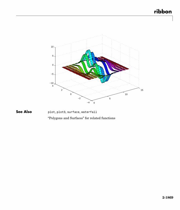
ribbon
2-1869
See Also plot, plot3, surface, waterfall
“Polygons and Surfaces” for related functions
0
5
10
15
−4
−2
0
2
4−10
−5
0
5
10

rmappdata
2-1870
2rmappdataPurpose Remove application-defined data
Syntax rmappdata(h,name)
Description rmappdata(h,name) removes the application-defined data name from the object specified by handle h.
See Also getappdata, isappdata, setappdata

rmdir
2-1871
2rmdirPurpose Remove directory
Graphical Interface
As an alternative to the rmdir function, use the delete feature in the Current Directory browser.
Syntax rmdir('dirname')rmdir('dirname','s')[status,message,messageid] = rmdir('dirname','s')
Description rmdir('dirname') removes the directory dirname from the current directory. If the directory is not empty, you must use the s argument. If dirname is not in the current directory, specify the relative path to the current directory or the full path for dirname.
rmdir('dirname','s') removes the directory dirname and its contents from the current directory. This removes all subdirectories and files in the current directory regardless of their write permissions.
[status, message, messageid] = rmdir('dirname','s') removes the directory dirname and its contents from the current directory, returning the status, a message, and the MATLAB error message ID (see error and lasterr). Here, status is 1 for success and is 0 for error, and message, messageid, and the s input argument are optional.
Examples Remove Empty DirectoryTo remove myfiles from the current directory, where myfiles is empty, type
rmdir('myfiles')
If the current directory is matlabr13/work, and myfiles is in d:/matlabr13/work/project/, use the relative path to myfiles
rmdir('project/myfiles')
or the full path to myfiles
rmdir('d:/matlabr13/work/project/myfiles')

rmdir
2-1872
Remove Directory and All ContentsTo remove myfiles, its subdirectories, and all files in the directories, assuming myfiles is in the current directory, type
rmdir('myfiles','s')
Remove Directory and Return ResultsTo remove myfiles from the current directory, type
[stat, mess, id]=rmdir('myfiles')
MATLAB returns
stat = 0
mess =
The directory is not empty.
id =
MATLAB:RMDIR:OSError
indicating the directory myfiles is not empty.
To remove myfiles and its contents, run
[stat, mess]=rmdir('myfiles','s')
and MATLAB returns
stat =
1
mess =
''
indicating myfiles and its contents were removed.

rmdir
2-1873
See Also cd, copyfile, delete, dir, error, fileattrib, filebrowser, lasterr, mkdir, movefile
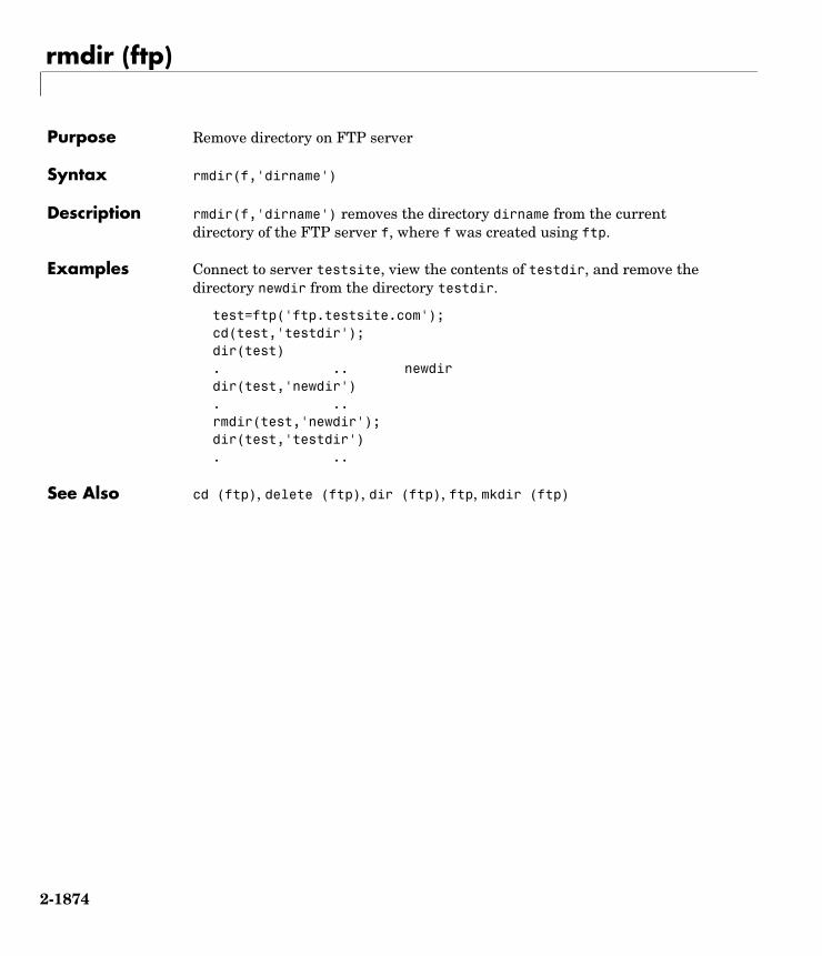
rmdir (ftp)
2-1874
2rmdir (ftp)Purpose Remove directory on FTP server
Syntax rmdir(f,'dirname')
Description rmdir(f,'dirname') removes the directory dirname from the current directory of the FTP server f, where f was created using ftp.
Examples Connect to server testsite, view the contents of testdir, and remove the directory newdir from the directory testdir.
test=ftp('ftp.testsite.com');cd(test,'testdir');dir(test). .. newdirdir(test,'newdir'). ..rmdir(test,'newdir');dir(test,'testdir'). ..
See Also cd (ftp), delete (ftp), dir (ftp), ftp, mkdir (ftp)

rmfield
2-1875
2rmfieldPurpose Remove structure fields
Syntax s = rmfield(s,'field')s = rmfield(s,FIELDS)
Description s = rmfield(s,'field') removes the specified field from the structure array s.
s = rmfield(s,FIELDS) removes more than one field at a time when FIELDS is a character array of field names or cell array of strings.
See Also fieldnames, setfield, getfield, isfield, orderfields, dynamic field names

rmpath
2-1876
2rmpathPurpose Remove directories from MATLAB search path
Graphical Interface
As an alternative to the rmpath function, use the Set Path dialog box. To open it, select Set Path from the File menu in the MATLAB desktop.
Syntax rmpath('directory')rmpath directory
Description rmpath('directory') removes the specified directory from the current MATLAB search path. Use the full pathname for directory.
rmpath directory is the unquoted form of the syntax.
Examples Remove /usr/local/matlab/mytools from the search path.
rmpath /usr/local/matlab/mytools
See Also addpath, cd, dir, genpath, matlabroot, partialpath, path, pathdef, pathsep, pathtool, rehash, restoredefaultpath, savepath, what
Search Path

root object
2-1877
2root objectPurpose Root object properties
Description The root is a graphics object that corresponds to the computer screen. There is only one root object and it has no parent. The children of the root object are figures.
The root object exists when you start MATLAB; you never have to create it and you cannot destroy it. Use set and get to access the root properties.
See Also diary, echo, figure, format, gcf, get, set
Object Hierarchy
Axes Uiobjects
Figure
Root

Root Properties
2-1878
2Root PropertiesModifying Properties
You can set and query graphics object properties in two ways:
• The Property Editor is an interactive tool that enables you to see and change object property values.
• The set and get commands enable you to set and query the values of properties.
To change the default values of properties, see Setting Default Property Values.
Root Properties This section lists property names along with the type of values each accepts. Curly braces enclose default values.
BusyAction cancel | queue
Not used by the root object.
ButtonDownFcn string
Not used by the root object.
CallbackObject handle (read only)
Handle of current callback’s object. This property contains the handle of the object whose callback routine is currently executing. If no callback routines are executing, this property contains the empty matrix [ ]. See also the gco command.
CaptureMatrix (obsolete)
This property has been superseded by the getframe command.
CaptureRect (obsolete)
This property has been superseded by the getframe command.
Children vector of handles
Handles of child objects. A vector containing the handles of all nonhidden figure objects (see HandleVisibility for more information). You can change the order of the handles and thereby change the stacking order of the figures on the display.
Clipping on | off
Clipping has no effect on the root object.

Root Properties
2-1879
CommandWindowSize [columns rows]
Current size of command window. This property contains the size of the MATLAB command window in a two-element vector. The first element is the number of columns wide and the second element is the number of rows tall.
CreateFcn
The root does not use this property.
CurrentFigure figure handle
Handle of the current figure window, which is the one most recently created, clicked in, or made current with the statement
figure(h)
which restacks the figure to the top of the screen, or
set(0,'CurrentFigure',h)
which does not restack the figures. In these statements, h is the handle of an existing figure. If there are no figure objects,
get(0,'CurrentFigure')
returns the empty matrix. Note, however, that gcf always returns a figure handle, and creates one if there are no figure objects.
DeleteFcn string
This property is not used, because you cannot delete the root object.
Diary on | off
Diary file mode. When this property is on, MATLAB maintains a file (whose name is specified by the DiaryFile property) that saves a copy of all keyboard input and most of the resulting output. See also the diary command.
DiaryFile string
Diary filename. The name of the diary file. The default name is diary.
Echo on | off
Script echoing mode. When Echo is on, MATLAB displays each line of a script file as it executes. See also the echo command.

Root Properties
2-1880
ErrorMessage string
Text of last error message. This property contains the last error message issued by MATLAB.
FixedWidthFontName font name
Fixed-width font to use for axes, text, and uicontrols whose FontName is set to FixedWidth. MATLAB uses the font name specified for this property as the value for axes, text, and uicontrol FontName properties when their FontName property is set to FixedWidth. Specifying the font name with this property eliminates the need to hardcode font names in MATLAB applications and thereby enables these applications to run without modification in locales where non-ASCII character sets are required. In these cases, MATLAB attempts to set the value of FixedWidthFontName to the correct value for a given locale.
MATLAB application developers should not change this property, but should create axes, text, and uicontrols with FontName properties set to FixedWidth when they want to use a fixed-width font for these objects.
MATLAB end users can set this property if they do not want to use the preselected value. In locales where Latin-based characters are used, Courier is the default.
Format short | shortE | long | longE | bank |hex | + | rat
Output format mode. This property sets the format used to display numbers. See also the format command.
• short — Fixed-point format with 5 digits
• shortE — Floating-point format with 5 digits
• shortG — Fixed- or floating-point format displaying as many significant figures as possible with 5 digits
• long — Scaled fixed-point format with 15 digits
• longE — Floating-point format with 15 digits
• longG — Fixed- or floating-point format displaying as many significant figures as possible with 15 digits
• bank — Fixed-format of dollars and cents
• hex — Hexadecimal format

Root Properties
2-1881
• + — Displays + and – symbols
• rat — Approximation by ratio of small integers
FormatSpacing compact | loose
Output format spacing (see also format command).
• compact — Suppress extra line feeds for more compact display.
• loose — Display extra line feeds for a more readable display.
HandleVisibility on | callback | off
This property is not useful on the root object.
HitTest on | off
This property is not useful on the root object.
Interruptible on | off
This property is not useful on the root object.
Language string
System environment setting.
MonitorPosition [x y width height;x y width height]
Width and height of primary and secondary monitors, in pixels. This property contains the width and height of each monitor connnected to your computer. The x and y values for the primary monitor are 0, 0 and the width and height of the monitor are specified in pixels.
The secondary monitor position is specified as
x = primary monitor width + 1y = primary monitor height + 1
Querying the value of the figure MonitorPosition on a multiheaded system returnes the position for each monitor on a separate line.
v = get(0,'MonitorPosition')v =
x y width height % Primary monitorx y width height % Secondary monitor
Note that MATLAB sets the value of the ScreenSize property to the combined size of the monitors.

Root Properties
2-1882
Parent handle
Handle of parent object. This property always contains the empty matrix, because the root object has no parent.
PointerLocation [x,y]
Current location of pointer. A vector containing the x- and y-coordinates of the pointer position, measured from the lower left corner of the screen. You can move the pointer by changing the values of this property. The Units property determines the units of this measurement.
This property always contains the instantaneous pointer location, even if the pointer is not in a MATLAB window. A callback routine querying the PointerLocation can get a different value than the location of the pointer when the callback was triggered. This difference results from delays in callback execution caused by competition for system resources.
PointerWindow handle (read only)
Handle of window containing the pointer. MATLAB sets this property to the handle of the figure window containing the pointer. If the pointer is not in a MATLAB window, the value of this property is 0. A callback routine querying the PointerWindow can get the wrong window handle if you move the pointer to another window before the callback executes. This error results from delays in callback execution caused by competition for system resources.
RecursionLimit integer
Number of nested M-file calls. This property sets a limit to the number of nested calls to M-files MATLAB will make before stopping (or potentially running out of memory). By default the value is set to a large value. Setting this property to a smaller value (something like 150, for example) should prevent MATLAB from running out of memory and will instead cause MATLAB to issue an error when the limit is reached.
ScreenDepth bits per pixel
Screen depth. The depth of the display bitmap (i.e., the number of bits per pixel). The maximum number of simultaneously displayed colors on the current graphics device is 2 raised to this power.
ScreenDepth supersedes the BlackAndWhite property. To override automatic hardware checking, set this property to 1. This value causes MATLAB to assume the display is monochrome. This is useful if MATLAB is running on
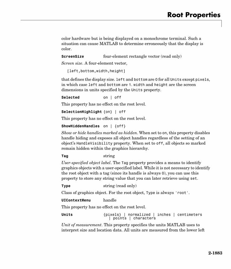
Root Properties
2-1883
color hardware but is being displayed on a monochrome terminal. Such a situation can cause MATLAB to determine erroneously that the display is color.
ScreenSize four-element rectangle vector (read only)
Screen size. A four-element vector,
[left,bottom,width,height]
that defines the display size. left and bottom are 0 for all Units except pixels, in which case left and bottom are 1. width and height are the screen dimensions in units specified by the Units property.
Selected on | off
This property has no effect on the root level.
SelectionHighlight on | off
This property has no effect on the root level.
ShowHiddenHandles on | off
Show or hide handles marked as hidden. When set to on, this property disables handle hiding and exposes all object handles regardless of the setting of an object’s HandleVisibility property. When set to off, all objects so marked remain hidden within the graphics hierarchy.
Tag string
User-specified object label. The Tag property provides a means to identify graphics objects with a user-specified label. While it is not necessary to identify the root object with a tag (since its handle is always 0), you can use this property to store any string value that you can later retrieve using set.
Type string (read only)
Class of graphics object. For the root object, Type is always 'root'.
UIContextMenu handle
This property has no effect on the root level.
Units pixels | normalized | inches | centimeters| points | characters
Unit of measurement. This property specifies the units MATLAB uses to interpret size and location data. All units are measured from the lower left

Root Properties
2-1884
corner of the screen. Normalized units map the lower left corner of the screen to (0,0) and the upper right corner to (1.0,1.0). inches, centimeters, and points are absolute units (one point equals 1/72 of an inch). Characters are units defined by characters from the default system font; the width of one unit is the width of the letter x, the height of one character is the distance between the baselines of two lines of text.
This property affects the PointerLocation and ScreenSize properties. If you change the value of Units, it is good practice to return it to its default value after completing your operation, so as not to affect other functions that assume Units is set to the default value.
UserData matrix
User-specified data. This property can be any data you want to associate with the root object. MATLAB does not use this property, but you can access it using the set and get functions.
Visible on | off
Object visibility. This property has no effect on the root object.

roots
2-1885
2rootsPurpose Polynomial roots
Syntax r = roots(c)
Description r = roots(c) returns a column vector whose elements are the roots of the polynomial c.
Row vector c contains the coefficients of a polynomial, ordered in descending powers. If c has n+1 components, the polynomial it represents is
.
Remarks Note the relationship of this function to p = poly(r), which returns a row vector whose elements are the coefficients of the polynomial. For vectors, roots and poly are inverse functions of each other, up to ordering, scaling, and roundoff error.
Examples The polynomial is represented in MATLAB as
p = [1 -6 -72 -27]
The roots of this polynomial are returned in a column vector by
r = roots(p)
r = 12.1229 -5.7345 -0.3884
Algorithm The algorithm simply involves computing the eigenvalues of the companion matrix:
A = diag(ones(n-1,1),-1);A(1,:) = -c(2:n+1)./c(1);eig(A)
It is possible to prove that the results produced are the exact eigenvalues of a matrix within roundoff error of the companion matrix A, but this does not mean that they are the exact roots of a polynomial with coefficients within roundoff error of those in c.
c1sn … cns cn 1++ + +
s3 6s2– 72s– 27–

roots
2-1886
See Also fzero, poly, residue

rose
2-1887
2rosePurpose Angle histogram
Syntax rose(theta)rose(theta,x)rose(theta,nbins)rose(axes_handles,...)h = rose(...)[tout,rout] = rose(...)
Description rose creates an angle histogram, which is a polar plot showing the distribution of values grouped according to their numeric range. Each group is shown as one bin.
rose(theta) plots an angle histogram showing the distribution of theta in 20 angle bins or less. The vector theta, expressed in radians, determines the angle of each bin from the origin. The length of each bin reflects the number of elements in theta that fall within a group, which ranges from 0 to the greatest number of elements deposited in any one bin.
rose(theta,x) uses the vector x to specify the number and the locations of bins. length(x) is the number of bins and the values of x specify the center angle of each bin. For example, if x is a five-element vector, rose distributes the elements of theta in five bins centered at the specified x values.
rose(theta,nbins) plots nbins equally spaced bins in the range [0, 2*pi]. The default is 20.
rose(axes_handle,...) plots into the axes with handle axes_handle instead of the current axes (gca).
h = rose(...) returns the handles of the line objects used to create the graph.
[tout,rout] = rose(...) returns the vectors tout and rout so polar(tout,rout) generates the histogram for the data. This syntax does not generate a plot.

rose
2-1888
Example Create a rose plot showing the distribution of 50 random numbers.
theta = 2*pi*rand(1,50);rose(theta)
See Also compass, feather, hist, line, polar
“Histograms” for related functions
Histograms in Polar Coordinates for another example
1
2
3
4
5
30
210
60
240
90
270
120
300
150
330
180 0

rosser
2-1889
2rosserPurpose Classic symmetric eigenvalue test problem
Syntax A = rosser
Description A = rosser returns the Rosser matrix. This matrix was a challenge for many matrix eigenvalue algorithms. But LAPACK's DSYEV routine used in MATLAB has no trouble with it. The matrix is 8-by-8 with integer elements. It has:
• A double eigenvalue
• Three nearly equal eigenvalues
• Dominant eigenvalues of opposite sign
• A zero eigenvalue
• A small, nonzero eigenvalue
Examples rosser
ans =
611 196 -192 407 -8 -52 -49 29 196 899 113 -192 -71 -43 -8 -44 -192 113 899 196 61 49 8 52 407 -192 196 611 8 44 59 -23 -8 -71 61 8 411 -599 208 208 -52 -43 49 44 -599 411 208 208 -49 -8 8 59 208 208 99 -911 29 -44 52 -23 208 208 -911 99

rot90
2-1890
2rot90Purpose Rotate matrix 90°
Syntax B = rot90(A)B = rot90(A,k)
Description B = rot90(A) rotates matrix A counterclockwise by 90 degrees.
B = rot90(A,k) rotates matrix A counterclockwise by k*90 degrees, where k is an integer.
Examples The matrix
X = 1 2 3 4 5 6 7 8 9
rotated by 90 degrees is
Y = rot90(X)Y = 3 6 9 2 5 8 1 4 7
See Also flipdim, fliplr, flipud

rotate
2-1891
2rotatePurpose Rotate object about a specified direction
Syntax rotate(h,direction,alpha)rotate(...,origin)
Description The rotate function rotates a graphics object in three-dimensional space, according to the right-hand rule.
rotate(h,direction,alpha) rotates the graphics object h by alpha degrees. direction is a two- or three-element vector that describes the axis of rotation in conjunction with the origin.
rotate(...,origin) specifies the origin of the axis of rotation as a three-element vector. The default origin is the center of the plot box.
Remarks The graphics object you want rotated must be a child of the same axes. The object’s data is modified by the rotation transformation. This is in contrast to view and rotate3d, which only modify the viewpoint.
The axis of rotation is defined by an origin and a point P relative to the origin. P is expressed as the spherical coordinates [theta phi] or as Cartesian coordinates.
The two-element form for direction specifies the axis direction using the spherical coordinates [theta phi]. theta is the angle in the x-y plane counterclockwise from the positive x-axis. phi is the elevation of the direction vector from the x-y plane.
Z
Y
X
P
originaxis of ro
tation

rotate
2-1892
The three-element form for direction specifies the axis direction using Cartesian coordinates. The direction vector is the vector from the origin to (X,Y,Z).
Examples Rotate a graphics object 180° about the x-axis.
h = surf(peaks(20));rotate(h,[1 0 0],180)
Rotate a surface graphics object 45° about its center in the z direction.
h = surf(peaks(20));zdir = [0 0 1];center = [10 10 0];rotate(h,zdir,45,center)
Remarks rotate changes the Xdata, Ydata, and Zdata properties of the appropriate graphics object.
See Also rotate3d, sph2cart, view
The axes CameraPosition, CameraTarget, CameraUpVector, CameraViewAngle
“Object Manipulation” for related functions
Z
Y
X
theta
P
phi
r

rotate3d
2-1893
2rotate3d Purpose Rotate 3-D view using mouse
Syntax rotate3d onrotate3d offrotate3drotate3d(figure_handle,...)rotate3d(axes_handle,...)
Description rotate3d on enables mouse-base rotation on all axes within the current figure.
rotate3d off disables interactive axes rotation in the current figure.
rotate3d toggles interactive axes rotation in the current figure.
rotate3d(figure_handle,...) enables rotation within the specified figure instead of the current figure.
rotate3d(axes_handle,...) enables rotation only in the specified axes.
Using rotate3dWhen enabled, rotate3d provides continuous rotation of axes and the objects it contains through mouse movement. A numeric readout appears in the lower left corner of the figure during rotation, showing the current azimuth and elevation of the axes. Releasing the mouse button removes the animated box and the readout.
You can also enable 3-D rotation from the figure Tools menu or the figure toolbar.
See Also camorbit, rotate, view
Object Manipulation for related functions

round
2-1894
2roundPurpose Round to nearest integer
Syntax Y = round(X)
Description Y = round(X) rounds the elements of X to the nearest integers. For complex X, the imaginary and real parts are rounded independently.
Examples a = [-1.9, -0.2, 3.4, 5.6, 7.0, 2.4+3.6i]
a = Columns 1 through 4 -1.9000 -0.2000 3.4000 5.6000 Columns 5 through 6 7.0000 2.4000 + 3.6000i
round(a)
ans = Columns 1 through 4 -2.0000 0 3.0000 6.0000 Columns 5 through 6 7.0000 2.0000 + 4.0000i
See Also ceil, fix, floor
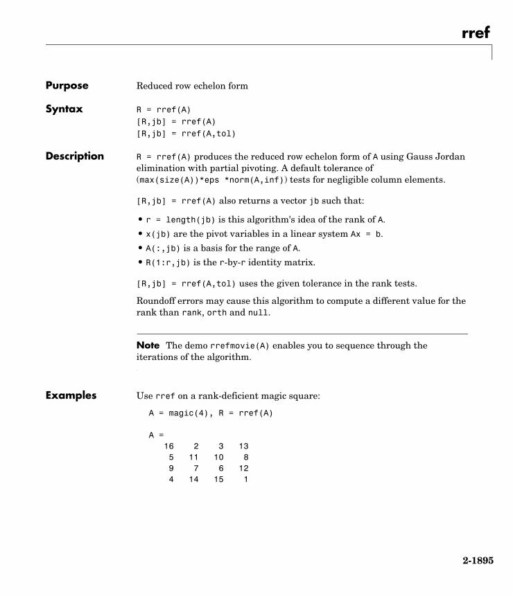
rref
2-1895
2rrefPurpose Reduced row echelon form
Syntax R = rref(A)[R,jb] = rref(A)[R,jb] = rref(A,tol)
Description R = rref(A) produces the reduced row echelon form of A using Gauss Jordan elimination with partial pivoting. A default tolerance of (max(size(A))*eps *norm(A,inf)) tests for negligible column elements.
[R,jb] = rref(A) also returns a vector jb such that:
• r = length(jb) is this algorithm's idea of the rank of A.
• x(jb) are the pivot variables in a linear system Ax = b.
• A(:,jb) is a basis for the range of A.
• R(1:r,jb) is the r-by-r identity matrix.
[R,jb] = rref(A,tol) uses the given tolerance in the rank tests.
Roundoff errors may cause this algorithm to compute a different value for the rank than rank, orth and null.
Note The demo rrefmovie(A) enables you to sequence through the iterations of the algorithm.
Examples Use rref on a rank-deficient magic square:
A = magic(4), R = rref(A)
A = 16 2 3 13 5 11 10 8 9 7 6 12 4 14 15 1

rref
2-1896
R = 1 0 0 1 0 1 0 3 0 0 1 -3 0 0 0 0
See Also inv, lu, rank

rsf2csf
2-1897
2rsf2csfPurpose Convert real Schur form to complex Schur form
Syntax [U,T] = rsf2csf(U,T)
Description The complex Schur form of a matrix is upper triangular with the eigenvalues of the matrix on the diagonal. The real Schur form has the real eigenvalues on the diagonal and the complex eigenvalues in 2-by-2 blocks on the diagonal.
[U,T] = rsf2csf(U,T) converts the real Schur form to the complex form.
Arguments U and T represent the unitary and Schur forms of a matrix A, respectively, that satisfy the relationships: A = U*T*U' and U'*U = eye(size(A)). See schur for details.
Examples Given matrix A,
1 1 1 3 1 2 1 1 1 1 3 1-2 1 1 4
with the eigenvalues
4.8121 1.9202 + 1.4742i 1.9202 + 1.4742i 1.3474
Generating the Schur form of A and converting to the complex Schur form
[u,t] = schur(A);[U,T] = rsf2csf(u,t)
yields a triangular matrix T whose diagonal (underlined here for readability) consists of the eigenvalues of A.
U =
-0.4916 -0.2756 - 0.4411i 0.2133 + 0.5699i -0.3428-0.4980 -0.1012 + 0.2163i -0.1046 + 0.2093i 0.8001-0.6751 0.1842 + 0.3860i -0.1867 - 0.3808i -0.4260-0.2337 0.2635 - 0.6481i 0.3134 - 0.5448i 0.2466

rsf2csf
2-1898
T =
4.8121 -0.9697 + 1.0778i -0.5212 + 2.0051i -1.0067 0 1.9202 + 1.4742i 2.3355 0.1117 + 1.6547i 0 0 1.9202 - 1.4742i 0.8002 + 0.2310i 0 0 0 1.3474
See Also schur

save
2-1899
2savePurpose Save workspace variables on disk
Graphical Interface
As an alternative to the save function, select Save Workspace As from the File menu in the MATLAB desktop, or use the Workspace browser.
Syntax savesave('filename')save('filename', 'var1', 'var2', ...)save('filename', '-struct', 's')save('filename', '-struct', 's', 'f1', 'f2', ...)save('-regexp', expr1, expr2, ...)save('..., 'format')save filename var1 var2 ...
Description save by itself stores all workspace variables in a binary format in the current directory in a file named matlab.mat. Retrieve the data with load. MAT-files are double-precision, binary, MATLAB format files. They can be created on one machine and later read by MATLAB on another machine with a different floating-point format, retaining as much accuracy and range as the different formats allow. They can also be manipulated by other programs external to MATLAB.
save('filename') stores all workspace variables in the current directory in filename.mat. To save to another directory, use the full pathname for the filename. If filename is the special string stdio, the save command sends the data as standard output.
save('filename', 'var1', 'var2', ...) saves only the specified workspace variables in filename.mat. Use the * wildcard to save only those variables that match the specified pattern. For example, save('A*') saves all variables that start with A.
save('filename', '-struct', 's') saves all fields of the scalar structure s as individual variables within the file filename.
save('filename', '-struct', 's', 'f1', 'f2', ...) saves as individual variables only those structure fields specified (s.f1, s.f2, ...).

save
2-1900
save('-regexp', expr1, expr2, ...) saves those variables that match any of the regular expressions expr1, expr2, etc.
save(..., 'format') enables you to make use of other data formats available with the save function. See the following table.
save filename var1 var2 ... is the command form of the syntax.
Remarks By default, MATLAB compresses the data it saves to MAT-files. MATLAB also uses Unicode character encoding when saving character data. Specify the -v6 option if you want to disable both of these features for a particular save operation. If you save data to a MAT-file that you intend to load using MATLAB Version 6 or earlier, then you must specify the -v6 option when saving.
To override the compression and Unicode setting for all of your MATLAB sessions, use the Preferences dialog box. Open the Preferences dialog and select General and then MAT-Files. To disable data compression and Unicode encoding, click Ensure backward compatibility (-v6). To turn these features back on, click Use default features (Unicode and compression). See “General Preferences for MATLAB” in the Desktop Tools and Development Environment documentation for more information.
Format How Data Is Stored
-append The specified existing MAT-file, appended to the end. See Remarks, below.
-ascii 8-digit ASCII format
-ascii -double 16-digit ASCII format
-ascii -tabs Delimits with tabs
-ascii -double -tabs 16-digit ASCII format, tab delimited
-mat Binary MAT-file form (default)
-v4 A format that MATLAB Version 4 can open
-v6 A format that MATLAB Version 6 and ear-lier can open

save
2-1901
For information on any of the following topics related to saving to MAT-files, see “Exporting Data to MAT-Files” in the “MATLAB Programming” documentation:
• Appending variables to an existing MAT-file
• Compressing data in the MAT-file
• Saving in ASCII format
• Saving in MATLAB Version 4 format
• Saving with Unicode character encoding
• Data storage requirements
• Saving from external programs
Examples Example 1Save all variables from the workspace in binary MAT-file test.mat:
save test.mat
Example 2Save variables p and q in binary MAT-file test.mat:
savefile = 'test.mat';p = rand(1, 10);q = ones(10);save(savefile, 'p', 'q')
Example 3Save the variables vol and temp in ASCII format to a file named june10:
save('d:\mymfiles\june10','vol','temp','-ASCII')
Example 4Save the fields of structure s1 as individual variables rather than as an entire structure.
s1.a = 12.7; s1.b = 'abc', [4 5; 6 7]; s1.c = 'Hello!';save newstruct.mat -struct s1;clear
Check what was saved to newstruct.mat:

save
2-1902
whos -file newstruct.mat Name Size Bytes Class
a 1x1 8 double array b 1x2 158 cell array c 1x6 12 char array
Grand total is 16 elements using 178 bytes
Read only the b field into the MATLAB workspace.
str = load('newstruct.mat', 'b')str = b: 'abc' [2x2 double]
Example 5Using regular expressions, save in MAT-file mydata.mat those variables with names that begin with Mon, Tue, or Wed:
save('mydata', '-regexp', '^Mon|^Tue|^Wed');
Here is another way of doing the same thing. In this case, there are three separate expression arguments:
save('mydata', '-regexp', '^Mon', '^Tue', '^Wed');
Example 6Save a 3000-by-3000 matrix uncompressed to file c1.mat, and compressed to file c2.mat. The compressed file uses about one quarter the disk space required to store the uncompressed data:
x = ones(3000);y = uint32(rand(3000) * 100);
save c1 x ysave c2 x y -compress
d1 = dir('c1.mat');d2 = dir('c2.mat');
d1.bytes

save
2-1903
ans = 45000240 % Size of the uncompressed datad2.bytesans = 11985634 % Size of the compressed data
d2.bytes/d1.bytesans = 0.2663 % Ratio of compressed to uncompressed
Example 7This example is similar to the last one, except that it saves one variable uncompressed, and then a second variable compressed to the same MAT-file. It then loads this data back into the MATLAB workspace:
x = ones(3000);y = uint32(rand(3000) * 100);
save c1 x;save c1 y -compress -append;
d = dir('c1.mat');d.bytesans = 20952950
clearload c1whos Name Size Bytes Class
x 3000x3000 72000000 double array y 3000x3000 36000000 uint32 array
Grand total is 18000000 elements using 108000000 bytes
See Also load, clear, diary, fprintf, fwrite, who, workspace

saveas
2-1904
2saveasPurpose Save figure or model using specified format
Syntax saveas(h,'filename.ext')saveas(h,'filename','format')
Description saveas(h,'filename.ext') saves the figure or model with the handle h to the file filename.ext. The format of the file is determined by the extension, ext. Allowable values for ext are listed in this table.
saveas(h,'filename','format') saves the figure or model with the handle h to the file called filename using the specified format. The filename can have an extension, but the extension is not used to define the file format. If no extension is specified, the standard extension corresponding to the specified format is automatically appended to the filename.
ext Values Format
ai Adobe Illustrator ‘88
bmp Windows bitmap
emf Enhanced metafile
eps EPS Level 1
fig MATLAB figure (invalid for Simulink models)
jpg JPEG image (invalid for Simulink models)
m MATLAB M-file (invalid for Simulink models)
pbm Portable bitmap
pcx Paintbrush 24-bit
pgm Portable Graymap
png Portable Network Graphics
ppm Portable Pixmap
tif TIFF image, compressed

saveas
2-1905
Allowable values for format are the extensions in the table above and the device types supported by print. The print device types include the formats listed in the table of extensions above as well as additional file formats. Use an extension from the table above or from the list of device types supported by print. When using the print device type to specify format for saveas, do not use the prefixed -d.
Remarks You can use open to open files saved using saveas with an m or fig extension. Other formats are not supported by open. The Save As dialog box you access from the figure window’s File menu uses saveas, limiting the file extensions to m and fig. The Export dialog box you access from the figure window’s File menu uses saveas with the format argument.
Examples Example 1 – Specify File ExtensionSave the current figure that you annotated using the Plot Editor to a file named pred_prey using the MATLAB fig format. This allows you to open the file pred_prey.fig at a later time and continue editing it with the Plot Editor.
saveas(gcf,'pred_prey.fig')
Example 2 – Specify File Format but No ExtensionSave the current figure, using Adobe Illustrator format, to the file logo. Use the ai extension from the above table to specify the format. The file created is logo.ai.
saveas(gcf,'logo', 'ai')
This is the same as using the Adobe Illustrator format from the print devices table, which is -dill; use doc print or help print to see the table for print device types. The file created is logo.ai. MATLAB automatically appends the ai extension for an Illustrator format file because no extension was specified.
saveas(gcf,'logo', 'ill')
Example 3 – Specify File Format and ExtensionSave the current figure to the file star.eps using the Level 2 Color PostScript format. If you use doc print or help print, you can see from the table for print device types that the device type for this format is -dpsc2. The file created is star.eps.

saveas
2-1906
saveas(gcf,'star.eps', 'psc2')
In another example, save the current model to the file trans.tiff using the TIFF format with no compression. From the table for print device types, you can see that the device type for this format is -dtiffn. The file created is trans.tiff.
saveas(gcf,'trans.tiff', 'tiffn')
See Also open, print
“Printing” for related functions

saveobj
2-1907
2saveobjPurpose Save an object to a MAT-file
Syntax B = saveobj(A)
Description B = saveobj(A) is called by the MATLAB save function when object A is saved to a MAT-file. This call executes the saveobj method for the object’s class, if such a method exists. The return value B is subsequently used by save to populate the MAT-file.
When you issue a save command on an object, MATLAB looks for a method called saveobj in the class directory. You can overload this method to modify the object before the save operation. For example, you could define a saveobj method that saves related data along with the object.
Remarks saveobj can be overloaded only for user objects. save will not call saveobj for a built-in datatype, such as double, even if @double/saveobj exists.
saveobj will be separately invoked for each object to be saved.
A child object does not inherit the saveobj method of its parent class. To implement saveobj for any class, including a class that inherits from a parent, you must define a saveobj method within that class directory.
Examples The following example shows a saveobj method written for the portfolio class. The method determines if a portfolio object has already been assigned an account number from a previous save operation. If not, saveobj calls getAccountNumber to obtain the number and assigns it to the account_number field. The contents of b is saved to the MAT-file.
function b = saveobj(a)if isempty(a.account_number) a.account_number = getAccountNumber(a);endb = a;
See Also save, load, loadobj

savepath
2-1908
2savepathPurpose Save current MATLAB search path to pathdef.m file
Graphical Interface
As an alternative to the savepath function, use the Set Path dialog box. To open it, select Set Path from the File menu in the MATLAB desktop.
Syntax savepathsavepath newfile
Description savepath saves the current MATLAB search path to pathdef.m. It returns
savepath newfile saves the current MATLAB search path to newfile, where newfile is in the current directory or is a relative or absolute path.
Examples The statement
savepath myfiles/pathdef.m
saves the current search path to the file pathdef.m, which is located in the myfiles directory in the MATLAB current directory.
Consider using savepath in your MATLAB finish.m file to save the path when you exit MATLAB.
See Also addpath, cd, dir, finish, genpath, matlabroot, partialpath, pathdef, pathsep, pathtool, rehash, restoredefaultpath, rmpath, savepath, startup, what
Search Path
0 If the file was saved successfully
1 If the save failed

scatter
2-1909
2scatterPurpose 2-D scatter/bubble graph
Syntax scatter(X,Y,S,C)scatter(X,Y)scatter(X,Y,S)scatter(...,markertype)scatter(...,'filled')scatter(...,'PropertyName',propertyvalue)scatter(axes_handle,...)h = scatter(...)hlines = scatter('v6',...)
Description scatter(X,Y,S,C) displays colored circles at the locations specified by the vectors X and Y (which must be the same size).
S determines the area of each marker (specified in points^2). S can be a vector the same length as X and Y or a scalar. If S is a scalar, MATLAB draws all the markers the same size.
C determines the colors of each marker. When C is a vector the same length as X and Y, the values in C are linearly mapped to the colors in the current colormap. When C is a length(X)-by-3 matrix, it specifies the colors of the markers as RGB values. C can also be a color string (see ColorSpec for a list of color string specifiers).
scatter(X,Y) draws the markers in the default size and color.
scatter(X,Y,S) draws the markers at the specified sizes (S) with a single color. This type of graph is also known as a bubble plot.
scatter(...,markertype) uses the marker type specified instead of 'o' (see LineSpec for a list of marker specifiers).
scatter(...,'filled') fills the markers.
scatter(...,'PropertyName',propertyvalue) creates the scatter graph, applying the specified property settings. See scattergroup properties for a description of properties.

scatter
2-1910
scatter(axes_handles,...) plots into the axes with handle axes_handle instead of the current axes (gca).
h = scatter(...) returns the handle of the scattergroup object created.
Backward Compatible Version
hpatch = scatter('v6',...) returns the handles to the patch objects created by scatter (see Patch Properties for a list of properties you can specify using the object handles and set).
See Plot Objects and Backward Compatibility for more information.
Examples load seamountscatter(x,y,5,z)
See Also scatter3, plot3
“Scatter/Bubble Plots” for related functions
See Triangulation and Interpolation of Scatter Data for related information.
See “Scattergroup Properties” for property descriptions
210.8 210.9 211 211.1 211.2 211.3 211.4 211.5 211.6 211.7 211.8−48.45
−48.4
−48.35
−48.3
−48.25
−48.2
−48.15
−48.1
−48.05
−48
−47.95

scatter3
2-1911
2scatter3Purpose 3-D scatter plot
Syntax scatter3(X,Y,Z,S,C)scatter3(X,Y,Z)scatter3(X,Y,Z,S)scatter3(...,markertype)scatter3(...,'filled')h = scatter3(...,)hpatch = scatter3('v6',...)
Description scatter3(X,Y,Z,S,C) displays colored circles at the locations specified by the vectors X, Y, and Z (which must all be the same size).
S determines the size of each marker (specified in points). S can be a vector the same length as X, Y, and Z or a scalar. If S is a scalar, MATLAB draws all the markers the same size.
C determines the colors of each marker. When C is a vector the same length as X, Y, and Z, the values in C are linearly mapped to the colors in the current colormap. When C is a length(X)-by-3 matrix, it specifies the colors of the markers as RGB values. C can also be a color string (see ColorSpec for a list of color string specifiers).
scatter3(X,Y,Z) draws the markers in the default size and color.
scatter3(X,Y,Z,S) draws the markers at the specified sizes (S) with a single color.
scatter3(...,markertype) uses the marker type specified instead of 'o' (see LineSpec for a list of marker specifiers).
scatter3(...,'filled') fills the markers.
h = scatter3(...) returns handles to the scattergroup objects created by scatter3. See “Scattergroup Properties” for property descriptions.
Backward Compatible Versionhpatch = scatter3('v6',...) returns the handles to the patch objects created by scatter3 (see Patch for a list of properties you can specify using the object handles and set).

scatter3
2-1912
Remarks Use plot3 for single color, single marker size 3-D scatter plots.
Examples [x,y,z] = sphere(16);X = [x(:)*.5 x(:)*.75 x(:)];Y = [y(:)*.5 y(:)*.75 y(:)];Z = [z(:)*.5 z(:)*.75 z(:)];S = repmat([1 .75 .5]*10,prod(size(x)),1);C = repmat([1 2 3],prod(size(x)),1);scatter3(X(:),Y(:),Z(:),S(:),C(:),'filled'), view(−60,60)
See Also scatter, plot3
See “Scattergroup Properties” for property descriptions
“Scatter/Bubble Plots” for related functions
−1
−0.5
0
0.5
1
−1
−0.5
0
0.5
1
−1
−0.5
0
0.5
1

Scattergroup Properties
2-1913
2Scattergroup PropertiesModifying Properties
You can set and query graphics object properties using the set and get commands or the Property Editor (propertyeditor).
Note that you cannot define default property values for scattergroup objects.
See Plot Objects for information on scattergroup objects.
Scattergroup Property Descriptions
This section provides a description of properties. Curly braces enclose default values.
BeingDeleted on | off Read Only
This object is being deleted. The BeingDeleted property provides a mechanism that you can use to determine whether objects are in the process of being deleted. MATLAB sets the BeingDeleted property to on when the object’s delete function callback is called (see the DeleteFcn property). It remains set to on while the delete function executes, after which the object no longer exists.
For example, an object’s delete function might call other functions that act on a number of different objects. These functions might not need to perform actions on objects if the objects are going to be deleted, and therefore can check the object’s BeingDeleted property before acting.
BusyAction cancel | queue
Callback routine interruption. The BusyAction property enables you to control how MATLAB handles events that potentially interrupt executing callbacks. If there is a callback function executing, callbacks invoked subsequently always attempt to interrupt it.
If the Interruptible property of the object whose callback is executing is set to on (the default), then interruption occurs at the next point where the event queue is processed. If the Interruptible property is off, the BusyAction property (of the object owning the executing callback) determines how MATLAB handles the event. The choices are
• cancel — Discard the event that attempted to execute a second callback routine.
• queue — Queue the event that attempted to execute a second callback routine until the current callback finishes.

Scattergroup Properties
2-1914
ButtonDownFcn string or function handle
Button press callback function. A callback that executes whenever you press a mouse button while the pointer is over the scattergroup object.
This property can be
• A string that is a valid MATLAB expression
• The name of an M-file
• A function handle
The expression executes in the MATLAB workspace.
See Function Handle Callbacks for information on how to use function handles to define the callbacks.
CData vector, m-by-3 matrix, ColorSpec
Color of markers. When CData is a vector the same length as XData and YData, the values in CData are linearly mapped to the colors in the current colormap. When CData is a length(XData)-by-3 matrix, it specifies the colors of the markers as RGB values. CData can also be a color string (see ColorSpec for a list of color string specifiers).
CDataSource string (MATLAB variable)
Link YData to MATLAB variable. Set this property to a MATLAB variable that, by default, is evaluated in the base workspace to generate the CData.
MATLAB reevaluates this property only when you set it. Therefore, a change to workspace variables appearing in an expression does not change CData.
You can use the refreshdata function to force an update of the object’s data. refreshdata also enables you to specify that the data source variable be evaluated in the workspace of a function from which you call refreshdata.
See the refreshdata reference page for more information.
Note If you change one data source property to a variable that contains data of a different dimension, you might cause the function to generate a warning and not render the graph until you have changed all data source properties to appropriate values.

Scattergroup Properties
2-1915
Children array of graphics object handles
Children of the scattergroup object. An array containing the handle of a patch object parented to the scattergroup object (whether visible or not).
Note that if a child object’s HandleVisibility property is set to callback or off, its handle does not show up in the stem Children property unless you set the Root ShowHiddenHandles property to on:
set(0,'ShowHiddenHandles','on')
Clipping on | off
Clipping mode. MATLAB clips scatter plots to the axes plot box by default. If you set Clipping to off, lines might be displayed outside the axes plot box.
CreateFcn string or function handle
Callback routine executed during object creation. This property defines a callback that executes when MATLAB creates a scattergroup object. You must specify the callback during the creation of the object. For example,
scatter(x,y,'CreateFcn',@CallbackFcn)
where @CallbackFcn is a function handle that references the callback function.
MATLAB executes this routine after setting all other scattergroup properties. Setting this property on an existing scattergroup object has no effect.
The handle of the object whose CreateFcn is being executed is accessible only through the root CallbackObject property, which you can query using gcbo.
See Function Handle Callbacks for information on how to use function handles to define the callback function.
DeleteFcn string or function handle
Callback executed during object deletion. A callback that executes when the scattergroup object is deleted (e.g., this might happen when you issue a delete command on the scattergroup object, its parent axes, or the figure containing it). MATLAB executes the callback before destroying the object’s properties so the callback routine can query these values.
The handle of the object whose DeleteFcn is being executed is accessible only through the root CallbackObject property, which can be queried using gcbo.

Scattergroup Properties
2-1916
See Function Handle Callbacks for information on how to use function handles to define the callback function.
See the BeingDeleted property for related information.
DisplayName string
Label used by plot legends. The legend and the plot browser use this text for labels for any scattergroup objects appearing in these legends.
EraseMode normal | none | xor | background
Erase mode. This property controls the technique MATLAB uses to draw and erase scatter child objects (the patch used to construct the scatter graph). Alternative erase modes are useful for creating animated sequences, where control of the way individual objects are redrawn is necessary to improve performance and obtain the desired effect.
• normal — Redraw the affected region of the display, performing the three-dimensional analysis necessary to ensure that all objects are rendered correctly. This mode produces the most accurate picture, but is the slowest. The other modes are faster, but do not perform a complete redraw and are therefore less accurate.
• none — Do not erase objects when they are moved or destroyed. While the objects are still visible on the screen after erasing with EraseMode none, you cannot print these objects because MATLAB stores no information about their former locations.
• xor— Draw and erase the object by performing an exclusive OR (XOR) with each pixel index of the screen behind it. Erasing the object does not damage the color of the objects behind it. However, the color of the erased object depends on the color of the screen behind it and it is correctly colored only when it is over the axes background color (or the figure background color if the axes Color property is set to none). That is, it isn’t erased correctly if there are objects behind it.
• background — Erase the graphics objects by redrawing them in the axes background color, (or the figure background color if the axes Color property is set to none). This damages other graphics objects that are behind the erased object, but the erased object is always properly colored.

Scattergroup Properties
2-1917
Printing with Nonnormal Erase ModesMATLAB always prints figures as if the EraseMode of all objects is normal. This means graphics objects created with EraseMode set to none, xor, or background can look different on screen than on paper. On screen, MATLAB can mathematically combine layers of colors (e.g., performing an XOR operation on a pixel color with that of the pixel behind it) and ignore three-dimensional sorting to obtain greater rendering speed. However, these techniques are not applied to the printed output.
Set the axes background color with the axes Color property. Set the figure background color with the figure Color property.
You can use the MATLAB getframe command or other screen capture applications to create an image of a figure containing nonnormal mode objects.
HandleVisibility on | callback | off
Control access to object’s handle by command-line users and GUIs. This property determines when an object’s handle is visible in its parent’s list of children. HandleVisibility is useful for preventing command-line users from accidentally accessing the scattergroup object.
• on — Handles are always visible when HandleVisibility is on.
• callback — Setting HandleVisibility to callback causes handles to be visible from within callback routines or functions invoked by callback routines, but not from within functions invoked from the command line. This provides a means to protect GUIs from command-line users, while allowing callback routines to have access to object handles.
• off — Setting HandleVisibility to off makes handles invisible at all times. This might be necessary when a callback invokes a function that might potentially damage the GUI (such as evaluating a user-typed string) and so temporarily hides its own handles during the execution of that function.
Functions Affected by Handle VisibilityWhen a handle is not visible in its parent’s list of children, it cannot be returned by functions that obtain handles by searching the object hierarchy or querying handle properties. This includes get, findobj, gca, gcf, gco, newplot, cla, clf, and close.

Scattergroup Properties
2-1918
Properties Affected by Handle VisibilityWhen a handle’s visibility is restricted using callback or off, the object’s handle does not appear in its parent’s Children property, figures do not appear in the root’s CurrentFigure property, objects do not appear in the root’s CallbackObject property or in the figure’s CurrentObject property, and axes do not appear in their parent’s CurrentAxes property.
Overriding Handle VisibilityYou can set the root ShowHiddenHandles property to on to make all handles visible regardless of their HandleVisibility settings (this does not affect the values of the HandleVisibility properties). See also findall.
Handle ValidityHandles that are hidden are still valid. If you know an object’s handle, you can set and get its properties and pass it to any function that operates on handles.
HitTest on | off
Selectable by mouse click. HitTest determines whether the scattergroup object can become the current object (as returned by the gco command and the figure CurrentObject property) as a result of a mouse click on the line objects that compose the stem plot. If HitTest is off, clicking the stemseries object selects the object below it (which is usually the axes containing it).
HitTestArea on | off
Select scattergroup object on markers or area of scatter graph. This property enables you to select scattergroup objects in two ways:
• Select by clicking on scatter markers (default).
• Select by clicking anywhere in the extent of the scatter graph.
When HitTestArea is off, you must click the scatter markers to select the scattergroup object. When HitTestArea is on, you can select the scattergroup object by clicking anywhere within the extent of the scatter graph (i.e., anywhere within a rectangle that encloses all the scatter markers).
Interruptible on | off
Callback routine interruption mode. The Interruptible property controls whether a scattergroup object callback can be interrupted by callbacks invoked subsequently.

Scattergroup Properties
2-1919
Only callbacks defined for the ButtonDownFcn property are affected by the Interruptible property. MATLAB checks for events that can interrupt a callback only when it encounters a drawnow, figure, getframe, or pause command in the routine. See the BusyAction property for related information.
Setting Interruptible to on allows any graphics object’s callback to interrupt callback routines originating from a stem property. Note that MATLAB does not save the state of variables or the display (e.g., the handle returned by the gca or gcf command) when an interruption occurs.
LineWidth width in points (default: 0.5 points)
Width of line that draws the edge of markers. You can set the thickness of the lines used to draw the markers to a value in points.
Marker character (see table)
Marker symbol. The Marker property specifies the type of markers that are displayed on the scatter graph. The following table shows supported markers.
Marker Specifier Description
+ Plus sign
o Circle
* Asterisk
. Point
x Cross
s Square
d Diamond
^ Upward-pointing triangle
v Downward-pointing triangle
> Right-pointing triangle
< Left-pointing triangle
p Five-pointed star (pentagram)

Scattergroup Properties
2-1920
MarkerEdgeColor ColorSpec | none | auto
Marker edge color. The color of the marker or the edge color for filled markers (circle, square, diamond, pentagram, hexagram, and the four triangles). ColorSpec defines the color to use. none specifies no color, which makes nonfilled markers invisible. auto uses the CData property to determine the MarkerEdgeColor.
MarkerFaceColor ColorSpec | none | auto
Marker face color. The fill color for markers that are closed shapes (circle, square, diamond, pentagram, hexagram, and the four triangles). ColorSpec defines the color to use. none makes the interior of the marker transparent, allowing the background to show through. auto sets the fill color to the axes color, or the figure color if the axes Color property is set to none (which is the factory default for axes objects).
Parent handle of axes, hggroup, or hgtransform
Parent of scattergroup object. This property contains the handle of the scattergroup object’s parent. The parent of a scattergroup object is the axes that contains it. You can reparent scattergroup objects to other axes, hggroup, or hgtransform objects.
See Objects That Can Contain Other Objects for more information on parenting graphics objects.
Selected on | off
Is object selected. When you set this property to on, MATLAB displays selection handles at the corners and midpoints if the SelectionHighlight property is also on (the default). You can, for example, define the ButtonDownFcn callback to set this property to on, thereby indicating that the scattergroup object is selected.
h Six-pointed star (hexagram)
none No marker (default)
Marker Specifier Description

Scattergroup Properties
2-1921
SelectionHighlight on | off
Objects are highlighted when selected. When the Selected property is on, MATLAB indicates the selected state by drawing selection handles on the scatter markers. When SelectionHighlight is off, MATLAB does not draw the handles.
SizeData square points
Size of markers in square points. This property specifies the area of the marker in the scatter graph in units of points. Since there are 72 points to one inch, to specify a marker that has an area of one square inch you would use a value of 72^2.
Tag string
User-specified object label. The Tag property provides a means to identify graphics objects with a user-specified label. This is particularly useful when you are constructing interactive graphics programs that would otherwise need to define object handles as global variables or pass them as arguments between callbacks.
For example, you might create a stemseries object and set the Tag property:
t = scatter(x,y,'Tag','scatter1')
When you want to access the scattergroup object, you can use findobj to find the scattergroup object’s handle. The following statement changes the MarkerFaceColor property of the object whose Tag is scatter1.
set(findobj('Tag','scatter1'),'MarkerFaceColor','red')
Type string (read only)
Type of graphics object. This property contains a string that identifies the class of the graphics object. For stemseries objects, Type is 'hggroup'. The following statement finds all the hggroup objects in the current axes.
t = findobj(gca,'Type','hggroup');
UIContextMenu handle of a uicontextmenu object
Associate a context menu with the scattergroup object. Assign this property the handle of a uicontextmenu object created in the scattergroup object’s parent figure. Use the uicontextmenu function to create the context menu. MATLAB

Scattergroup Properties
2-1922
displays the context menu whenever you right-click over the scattergroup object.
UserData array
User-specified data. This property can be any data you want to associate with the scattergroup object (including cell arrays and structures). The scattergroup object does not set values for this property, but you can access it using the set and get functions.
Visible on | off
Visibility of scattergroup object and its children. By default, scattergroup object visibility is on. This means all children of the scattergroup object are visible unless the child object’s Visible property is set to off. Setting a scattergroup object’s Visible property to off also makes its children invisible.
XData array
X-coordinates of scatter markers. The scatter function draws individual markers at each x-axis location in the XData array. The input argument x in the scatter function calling syntax assigns values to XData.
XDataSource string (MATLAB variable)
Link XData to MATLAB variable. Set this property to a MATLAB variable that, by default, is evaluated in the base workspace to generate the XData.
MATLAB reevaluates this property only when you set it. Therefore, a change to workspace variables appearing in an expression does not change XData.
You can use the refreshdata function to force an update of the object’s data. refreshdata also enables you to specify that the data source variable be evaluated in the workspace of a function from which you call refreshdata.
See the refreshdata reference page for more information.
Note If you change one data source property to a variable that contains data of a different dimension, you might cause the function to generate a warning and not render the graph until you have changed all data source properties to appropriate values.

Scattergroup Properties
2-1923
YData scalar, vector, or matrix
Y-coordinates of scatter markers. The scatter function draws individual markers at each y-axis location in the YData array.
The input argument y in the scatter function calling syntax assigns values to YData.
YDataSource string (MATLAB variable)
Links YData to MATLAB variable. Set this property to a MATLAB variable that, by default, is evaluated in the base workspace to generate the YData.
MATLAB reevaluates this property only when you set it. Therefore, a change to workspace variables appearing in an expression does not change YData.
You can use the refreshdata function to force an update of the object’s data. refreshdata also enables you to specify that the data source variable be evaluated in the workspace of a function from which you call refreshdata.
See the refreshdata reference page for more information.
Note If you change one data source property to a variable that contains data of a different dimension, you might cause the function to generate a warning and not render the graph until you have changed all data source properties to appropriate values.
ZData vector of coordinates
Z-coordinates. A vector of z-coordinates defining the scattergroup object. XData and YData must be the same length.
ZDataSource string (MATLAB variable)
Link ZData to MATLAB variable. Set this property to a MATLAB variable that, by default, is evaluated in the base workspace to generate the ZData.
MATLAB reevaluates this property only when you set it. Therefore, a change to workspace variables appearing in an expression does not change ZData.
You can use the refreshdata function to force an update of the object’s data. refreshdata also enables you to specify that the data source variable be evaluated in the workspace of a function from which you call refreshdata.

Scattergroup Properties
2-1924
See the refreshdata reference page for more information.
Note If you change one data source property to a variable that contains data of a different dimension, you might cause the function to generate a warning and not render the graph until you have changed all data source properties to appropriate values.
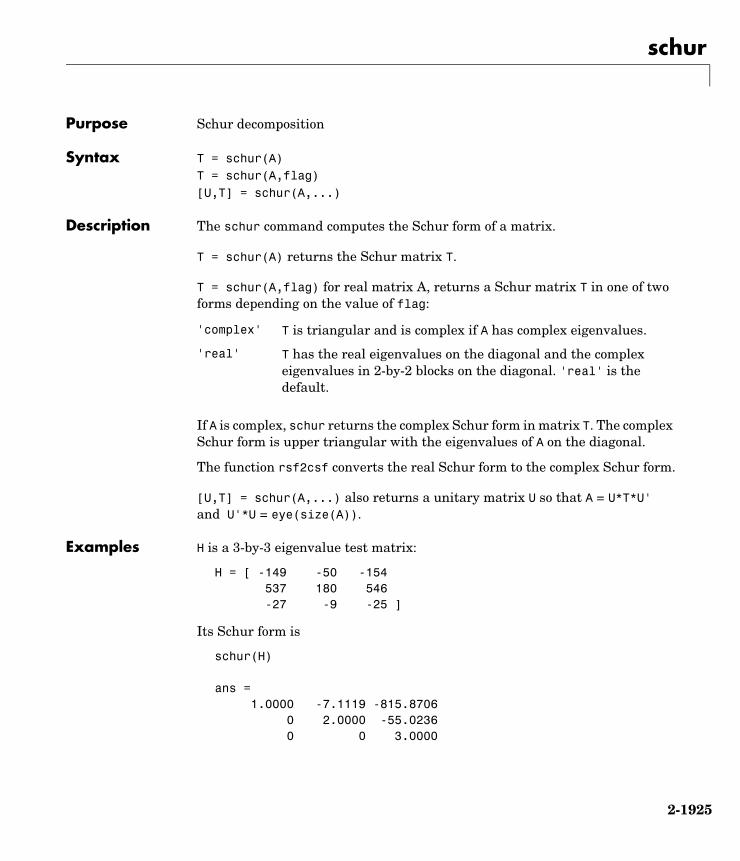
schur
2-1925
2schurPurpose Schur decomposition
Syntax T = schur(A)T = schur(A,flag)[U,T] = schur(A,...)
Description The schur command computes the Schur form of a matrix.
T = schur(A) returns the Schur matrix T.
T = schur(A,flag) for real matrix A, returns a Schur matrix T in one of two forms depending on the value of flag:
If A is complex, schur returns the complex Schur form in matrix T. The complex Schur form is upper triangular with the eigenvalues of A on the diagonal.
The function rsf2csf converts the real Schur form to the complex Schur form.
[U,T] = schur(A,...) also returns a unitary matrix U so that A = U*T*U' and U'*U = eye(size(A)).
Examples H is a 3-by-3 eigenvalue test matrix:
H = [ -149 -50 -154 537 180 546 -27 -9 -25 ]
Its Schur form is
schur(H)
ans = 1.0000 -7.1119 -815.8706 0 2.0000 -55.0236 0 0 3.0000
'complex' T is triangular and is complex if A has complex eigenvalues.
'real' T has the real eigenvalues on the diagonal and the complex eigenvalues in 2-by-2 blocks on the diagonal. 'real' is the default.

schur
2-1926
The eigenvalues, which in this case are 1, 2, and 3, are on the diagonal. The fact that the off-diagonal elements are so large indicates that this matrix has poorly conditioned eigenvalues; small changes in the matrix elements produce relatively large changes in its eigenvalues.
Algorithm schur uses LAPACK routines to compute the Schur form of a matrix:
See Also eig, hess, qz, rsf2csf
References [1] Anderson, E., Z. Bai, C. Bischof, S. Blackford, J. Demmel, J. Dongarra, J. Du Croz, A. Greenbaum, S. Hammarling, A. McKenney, and D. Sorensen, LAPACK User’s Guide (http://www.netlib.org/lapack/lug/lapack_lug.html), Third Edition, SIAM, Philadelphia, 1999.
Matrix A Routine
Real symmetric DSYTRD, DSTEQRDSYTRD, DORGTR, DSTEQR (with output U)
Real nonsymmetric DGEHRD, DHSEQRDGEHRD, DORGHR, DHSEQR (with output U)
Complex Hermitian ZHETRD, ZSTEQRZHETRD, ZUNGTR, ZSTEQR (with output U)
Non-Hermitian ZGEHRD, ZHSEQRZGEHRD, ZUNGHR, ZHSEQR (with output U)

script
2-1927
2scriptPurpose Script M-files
Description A script file is an external file that contains a sequence of MATLAB statements. By typing the filename, you can obtain subsequent MATLAB input from the file. Script files have a filename extension of .m and are often called M-files.
Scripts are the simplest kind of M-file. They are useful for automating blocks of MATLAB commands, such as computations you have to perform repeatedly from the command line. Scripts can operate on existing data in the workspace, or they can create new data on which to operate. Although scripts do not return output arguments, any variables that they create remain in the workspace, so you can use them in further computations. In addition, scripts can produce graphical output using commands like plot.
Scripts can contain any series of MATLAB statements. They require no declarations or begin/end delimiters.
Like any M-file, scripts can contain comments. Any text following a percent sign (%) on a given line is comment text. Comments can appear on lines by themselves, or you can append them to the end of any executable line.
See Also echo, function, type

sec
2-1928
2secPurpose Secant of an argument in radians
Syntax Y = sec(X)
Description The sec function operates element-wise on arrays. The function’s domains and ranges include complex values. All angles are in radians.
Y = sec(X) returns an array the same size as X containing the secant of the elements of X.
Examples Graph the secant over the domains and .
x1 = -pi/2+0.01:0.01:pi/2-0.01; x2 = pi/2+0.01:0.01:(3*pi/2)-0.01; plot(x1,sec(x1),x2,sec(x2)), grid on
The expression sec(pi/2) does not evaluate as infinite but as the reciprocal of the floating-point accuracy eps, because pi is a floating-point approximation to the exact value of .
Definition The secant can be defined as
π– 2⁄ x π 2⁄< < π 2⁄ x 3π 2⁄< <
−2 −1 0 1 2 3 4 5−150
−100
−50
0
50
100
150
π
sec z( ) 1cos z( )----------------=

sec
2-1929
Algorithm sec uses FDLIBM, which was developed at SunSoft, a Sun Microsystems, Inc. business, by Kwok C. Ng, and others. For information about FDLIBM, see http://www.netlib.org.
See Also asec, asech, eps, pi, secd, sech

secd
2-1930
2secdPurpose Secant of an argument in degrees
Syntax Y = secd(X)
Description Y = secd(X) is the secant of the elements of X, expressed in degrees. For odd integers n, secd(n*90) is infinite, whereas sec(n*pi/2) is large but finite, reflecting the accuracy of the floating point value of pi.
See Also asecd, sec

sech
2-1931
2sechPurpose Hyperbolic secant
Syntax Y = sech(X)
Description The sech function operates element-wise on arrays. The function’s domains and ranges include complex values. All angles are in radians.
Y = sech(X) returns an array the same size as X containing the hyperbolic secant of the elements of X.
Examples Graph the hyperbolic secant over the domain
x = -2*pi:0.01:2*pi; plot(x,sech(x)), grid on
Algorithm sech uses this algorithm.
Definition The secant can be defined as
2π– x 2π.≤ ≤
−8 −6 −4 −2 0 2 4 6 80
0.1
0.2
0.3
0.4
0.5
0.6
0.7
0.8
0.9
1
z( )sech 1z( )cosh
--------------------=
z( )sech 1z( )cosh
--------------------=

sech
2-1932
Algorithm sec uses FDLIBM, which was developed at SunSoft, a Sun Microsystems, Inc. business, by Kwok C. Ng, and others. For information about FDLIBM, see http://www.netlib.org.
See Also asec, asech, sec

selectmoveresize
2-1933
2selectmoveresizePurpose Select, move, resize, or copy axes and uicontrol graphics objects
Syntax A = selectmoveresize;set(h,'ButtonDownFcn','selectmoveresize')
Description selectmoveresize is useful as the callback routine for axes and uicontrol button down functions. When executed, it selects the object and allows you to move, resize, and copy it.
For example, this statement sets the ButtonDownFcn of the current axes to selectmoveresize:
set(gca,'ButtonDownFcn','selectmoveresize')
A = selectmoveresize returns a structure array containing
• A.Type: a string containing the action type, which can be Select, Move, Resize, or Copy
• A.Handles: a list of the selected handles, or, for a Copy, an m-by-2 matrix containing the original handles in the first column and the new handles in the second column
See Also The ButtonDownFcn of axes and uicontrol graphics objects
“Object Manipulation” for related functions
semilogx, semilogy
2-1934
2semilogx, semilogy Purpose Semilogarithmic plots
Syntax semilogx(Y)semilogx(X1,Y1,...)semilogx(X1,Y1,LineSpec,...)semilogx(...,'PropertyName',PropertyValue,...)h = semilogx(...)hlines = semilogx('v6',...)semilogy(...)h = semilogy(...)hlines = semilogx('v6',...)
Description semilogx and semilogy plot data as logarithmic scales for the x- and y-axis, respectively, logarithmic.
semilogx(Y) creates a plot using a base 10 logarithmic scale for the x-axis and a linear scale for the y-axis. It plots the columns of Y versus their index if Y contains real numbers. semilogx(Y) is equivalent to semilogx(real(Y), imag(Y)) if Y contains complex numbers. semilogx ignores the imaginary component in all other uses of this function.
semilogx(X1,Y1,...) plots all Xn versus Yn pairs. If only Xn or Yn is a matrix, semilogx plots the vector argument versus the rows or columns of the matrix, depending on whether the vector’s row or column dimension matches the matrix.
semilogx(X1,Y1,LineSpec,...) plots all lines defined by the Xn,Yn,LineSpec triples. LineSpec determines line style, marker symbol, and color of the plotted lines.
semilogx(...,'PropertyName',PropertyValue,...) sets property values for all lineseries graphics objects created by semilogx.
semilogy(...) creates a plot using a base 10 logarithmic scale for the y-axis and a linear scale for the x-axis.
h = semilogx(...) and h = semilogy(...) return a vector of handles to lineseries graphics objects, one handle per line.

semilogx, semilogy
2-1935
Backward Compatible Version
hlines = semilogx('v6',...) and hlines = semilogy('v6',...) return the handles to line objects instead of lineseries objects.
Remarks If you do not specify a color when plotting more than one line, semilogx and semilogy automatically cycle through the colors and line styles in the order specified by the current axes ColorOrder and LineStyleOrder properties.
You can mix Xn,Yn pairs with Xn,Yn,LineSpec triples; for example,
semilogx(X1,Y1,X2,Y2,LineSpec,X3,Y3)
Examples Create a simple semilogy plot.
x = 0:.1:10;semilogy(x,10.^x)
See Also line, LineSpec, loglog, plot“Basic Plots and Graphs” for related functions
0 1 2 3 4 5 6 7 8 9 1010
0
101
102
103
104
105
106
107
108
109
1010
sendmail
2-1936
2sendmailPurpose Send e-mail message to list of e-mail addresses
Syntax sendmail('recipients','subject')sendmail('recipients','subject','message','attachments')
Description sendmail('recipients','subject') sends e-mail to recipients with the specified subject. For recipients, use a string for a single address, or a cell array of strings for multiple addresses.
sendmail('recipients','subject','message','attachments') sends message to recipients with the specified subject. For recipients, use a string for a single address, or a cell array of strings for multiple addresses. For message, use a string or cell array. When message is a string, the text automatically wraps at 75 characters. When message is a cell array, it does not wrap but rather each cell is a new line. To force text to start on a new line in strings or cells, use 10, as shown in the “Example of sendmail with New Lines Specified” on page 2-1937. Specify attachments as a cell array of files to send along with message.
To use sendmail, you must set the preferences for your e-mail server (Internet SMTP server) and your e-mail address must be set. MATLAB tries to read the SMTP mail server from your system registry, but if it cannot, it results in an error. In this event, identify the outgoing mail server for your electronic mail application, which is usually listed in the application’s preferences, or, consult your e-mail system administrator. Then provide the information to MATLAB using
setpref('Internet','SMTP_Server','myserver.myhost.com');
If you cannot easily determine your e-mail server, try using mail, as in
setpref('Internet','SMTP_Server','mail');
which might work because mail is often a default for mail systems.
Similarly, if MATLAB cannot determine your e-mail address and produces an error, specify your e-mail address using
setpref('Internet','E_mail','[email protected]');

sendmail
2-1937
Note The sendmail function does not support email servers that require authentication.
Examples Example of sendmail with Two Attachmentssendmail('[email protected]','Test subject','Test message','directory/attach1.html','attach2.doc');
Example of sendmail with New Lines SpecifiedThis mail message forces the message to start new lines after each 10.
sendmail('[email protected]','New subject', ...['Line1 of message' 10 'Line2 of message' 10 ... 'Line3 of message' 10 'Line4 of message']);
The resulting message is
Line1 of messageLine2 of messageLine3 of message Line4 of message

set
2-1938
2setPurpose Set object properties
Syntax set(H,'PropertyName',PropertyValue,...)set(H,a)set(H,pn,pv...)set(H,pn,<m-by-n cell array>)a= set(h)a= set(0,'FactoryObjectTypePropertyName')a= set(h,'Default')a= set(h,'DefaultObjectTypePropertyName')<cell array> = set(h,'PropertyName')
Description set(H,'PropertyName',PropertyValue,...) sets the named properties to the specified values on the object(s) identified by H. H can be a vector of handles, in which case set sets the properties’ values for all the objects.
set(H,a) sets the named properties to the specified values on the object(s) identified by H. a is a structure array whose field names are the object property names and whose field values are the values of the corresponding properties.
set(H,pn,pv,...) sets the named properties specified in the cell array pn to the corresponding value in the cell array pv for all objects identified in H.
set(H,pn,<m-by-n cell array>) sets n property values on each of m graphics objects, where m = length(H) and n is equal to the number of property names contained in the cell array pn. This allows you to set a given group of properties to different values on each object.
a = set(h) returns the user-settable properties and possible values for the object identified by h. a is a structure array whose field names are the object’s property names and whose field values are the possible values of the corresponding properties. If you do not specify an output argument, MATLAB displays the information on the screen. h must be scalar.
a = set(0,'FactoryObjectTypePropertyName') returns the possible values of the named property for the specified object type, if the values are strings. The argument FactoryObjectTypePropertyName is the word Factory concatenated with the object type (e.g., axes) and the property name (e.g., CameraPosition).

set
2-1939
a = set(h,'Default') returns the names of properties having default values set on the object identified by h. set also returns the possible values if they are strings. h must be scalar.
a = set(h,'DefaultObjectTypePropertyName') returns the possible values of the named property for the specified object type, if the values are strings. The argument DefaultObjectTypePropertyName is the word Default concatenated with the object type (e.g., axes) and the property name (e.g., CameraPosition). For example, DefaultAxesCameraPosition. h must be scalar.
pv = set(h,'PropertyName') returns the possible values for the named property. If the possible values are strings, set returns each in a cell of the cell array pv. For other properties, set returns an empty cell array. If you do not specify an output argument, MATLAB displays the information on the screen. h must be scalar.
Remarks You can use any combination of property name/property value pairs, structure arrays, and cell arrays in one call to set.
Examples Set the Color property of the current axes to blue.
set(gca,'Color','b')
Change all the lines in a plot to black.
plot(peaks)set(findobj('Type','line'),'Color','k')
You can define a group of properties in a structure to better organize your code. For example, these statements define a structure called active, which contains a set of property definitions used for the uicontrol objects in a particular figure. When this figure becomes the current figure, MATLAB changes colors and enables the controls.
active.BackgroundColor = [.7 .7 .7];active.Enable = 'on';active.ForegroundColor = [0 0 0];
if gcf == control_fig_handleset(findobj(control_fig_handle,'Type','uicontrol'),active)
end

set
2-1940
You can use cell arrays to set properties to different values on each object. For example, these statements define a cell array to set three properties,
PropName(1) = 'BackgroundColor';PropName(2) = 'Enable';PropName(3) = 'ForegroundColor';
These statements define a cell array containing three values for each of three objects (i.e., a 3-by-3 cell array).
PropVal(1,1) = [.5 .5 .5]; PropVal(1,2) = 'off'; PropVal(1,3) = [.9 .9 .9];
PropVal(2,1) = [1 0 0]; PropVal(2,2) = 'on'; PropVal(2,3) = [1 1 1];
PropVal(3,1) = [.7 .7 .7]; PropVal(3,2) = 'on'; PropVal(3,3) = [0 0 0];
Now pass the arguments to set,
set(H,PropName,PropVal)
where length(H) = 3 and each element is the handle to a uicontrol.
Setting Different Values for the Same Property on Multiple ObjectsSuppose you want to set the value of the Tag property on five line objects, each to a different value. Note how the value cell array needs to be transposed to have the proper shape.
h = plot(rand(5));set(h,'Tag','line1','line2','line3','line4','line5'')
See Also findobj, gca, gcf, gco, gcbo, get
“Finding and Identifying Graphics Objects” for related functions

set (timer)
2-1941
2set (timer)Purpose Configure or display timer object properties
Syntax set(obj)prop_struct = set(obj)set(obj,'PropertyName')prop_cell = set(obj,'PropertyName')set(obj,'PropertyName',PropertyValue,...)set(obj,S)set(obj,PN,PV)
Description set(obj) displays property names and their possible values for all configurable properties of timer object obj. obj must be a single timer object.
prop_struct = set(obj) returns the property names and their possible values for all configurable properties of timer object obj. obj must be a single timer object. The return value, prop_struct, is a structure whose field names are the property names of obj, and whose values are cell arrays of possible property values or empty cell arrays if the property does not have a finite set of possible string values.
set(obj,'PropertyName') displays the possible values for the specified property, PropertyName, of timer object obj. obj must be a single timer object.
prop_cell=set(obj,'PropertyName') returns the possible values for the specified property, PropertyName, of timer object obj. obj must be a single timer object. The returned array, prop_cell, is a cell array of possible value strings or an empty cell array if the property does not have a finite set of possible string values.
set(obj,'PropertyName',PropertyValue,...) configures the property, PropertyName, to the specified value, PropertyValue, for timer object obj. You can specify multiple property name/property value pairs in a single statement. obj can be a single timer object or a vector of timer objects, in which case set configures the property values for all the timer objects specified.
set(obj,S) configures the properties of obj, with the values specified in S, where S is a structure whose field names are object property names.
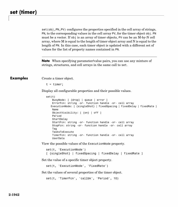
set (timer)
2-1942
set(obj,PN,PV) configures the properties specified in the cell array of strings, PN, to the corresponding values in the cell array PV, for the timer object obj. PN must be a vector. If obj is an array of timer objects, PV can be an M-by-N cell array, where M is equal to the length of timer object array and N is equal to the length of PN. In this case, each timer object is updated with a different set of values for the list of property names contained in PN.
Note When specifying parameter/value pairs, you can use any mixture of strings, structures, and cell arrays in the same call to set.
Examples Create a timer object.
t = timer;
Display all configurable properties and their possible values.
set(t)BusyMode: [ drop | queue | error ]
ErrorFcn: string -or- function handle -or- cell array ExecutionMode: [ singleShot | fixedSpacing | fixedDelay | fixedRate ] Name ObjectVisibility: [ on | off ] Period StartDelay StartFcn: string -or- function handle -or- cell array StopFcn: string -or- function handle -or- cell array Tag TasksToExecute TimerFcn: string -or- function handle -or- cell array UserData
View the possible values of the ExecutionMode property.
set(t, 'ExecutionMode')[ singleShot | fixedSpacing | fixedDelay | fixedRate ]
Set the value of a specific timer object property.
set(t, 'ExecutionMode', 'FixedRate')
Set the values of several properties of the timer object.
set(t, 'TimerFcn', 'callbk', 'Period', 10)

set (timer)
2-1943
Use a cell array to specify the names of the properties you want to set and another cell array to specify the values of these properties.
set(t, 'StartDelay', 'Period', 30, 30)
See Also timer, get

setappdata
2-1944
2setappdataPurpose Set application-defined data
Syntax setappdata(h,name,value)
Description setappdata(h,name,value) sets application-defined data for the object with handle h. The application-defined data, which is created if it does not already exist, is assigned a name and a value. value can be any type of data.
See Also getappdata, isappdata, rmappdata
Purpose Return the set difference of two vectors
Syntax c = setdiff(A, B)c = setdiff(A, B, 'rows')[c, i] = setdiff(...)
Description c = setdiff(A, B) returns the values in A that are not in B. The resulting vector is sorted in ascending order. In set theory terms, c = A - B. A and B can be cell arrays of strings.
c = setdiff(A, B, 'rows'), when A and B are matrices with the same number of columns, returns the rows from A that are not in B.
[c,i] = setdiff(...) also returns an index vector index such that c = a(i) or c = a(i,:).
Examples A = magic(5);B = magic(4);[c, i] = setdiff(A(:), B(:));c' = 17 18 19 20 21 22 23 24 25i' = 1 10 14 18 19 23 2 6 15
See Also intersect, ismember, issorted, setxor, union, unique

setdiff
2-1945
2setdiffPurpose Return the set difference of two vectors
Syntax c = setdiff(A, B)c = setdiff(A, B, 'rows')[c, i] = setdiff(...)
Description c = setdiff(A, B) returns the values in A that are not in B. The resulting vector is sorted in ascending order. In set theory terms, c = A - B. A and B can be cell arrays of strings.
c = setdiff(A, B, 'rows'), when A and B are matrices with the same number of columns, returns the rows from A that are not in B.
[c,i] = setdiff(...) also returns an index vector index such that c = a(i) or c = a(i,:).
Examples A = magic(5);B = magic(4);[c, i] = setdiff(A(:), B(:));c' = 17 18 19 20 21 22 23 24 25i' = 1 10 14 18 19 23 2 6 15
See Also intersect, ismember, issorted, setxor, union, unique

setfield
2-1946
2setfieldPurpose Set field of structure array
Syntax s = setfield(s, 'field', v)s = setfield(s, i,j, 'field', k ,v)
Description s = setfield(s, 'field', v), where s is a 1-by-1 structure, sets the contents of the specified field to the value v. This is equivalent to the syntax s.field = v.
s = setfield(s, i,j, 'field', k, v) sets the contents of the specified field to the value v. This is equivalent to the syntax s(i,j).field(k) = v. All subscripts must be passed as cell arrays — that is, they must be enclosed in curly braces (similar toi,j and k above). Pass field references as strings.
Remarks In many cases, you can use dynamic field names in place of the getfield and setfield functions. Dynamic field names express structure fields as variable expressions that MATLAB evaluates at run-time. See Technical Note 32236 for information about using dynamic field names versus the getfield and setfield functions.
Examples Given the structure
mystr(1,1).name = 'alice';mystr(1,1).ID = 0;mystr(2,1).name = 'gertrude';mystr(2,1).ID = 1;
You can change the name field of mystr(2,1) using
mystr = setfield(mystr, 2,1, 'name', 'ted');mystr(2,1).name
ans =
ted
The following example sets fields of a structure using setfield with variable and quoted field names and additional subscripting arguments.
class = 5; student = 'John_Doe';
setfield
2-1947
grades_Doe = [85, 89, 76, 93, 85, 91, 68, 84, 95, 73];grades = [];
grades = setfield(grades, class, student, 'Math', ... 10, 21:30, grades_Doe);
You can check the outcome using the standard structure syntax.
grades(class).John_Doe.Math(10, 21:30)
ans =
85 89 76 93 85 91 68 84 95 73
See Also getfield, fieldnames, isfield, orderfields, rmfield, dynamic field names

setstr
2-1948
2setstrPurpose Set string flag
Description This MATLAB 4 function has been renamed char in MATLAB 5.

setxor
2-1949
2setxorPurpose Set exclusive OR of two vectors
Syntax c = setxor(A, B)c = setxor(A, B, 'rows')[c, ia, ib] = setxor(...)
Description c = setxor(A, B) returns the values that are not in the intersection of A and B. The resulting vector is sorted. A and B can be cell arrays of strings.
c = setxor(A, B, 'rows'), when A and B are matrices with the same number of columns, returns the rows that are not in the intersection of A and B.
[c, ia, ib] = setxor(...) also returns index vectors ia and ib such that c is a sorted combination of the elements c = a(ia) and c = b(ib) or, for row combinations, c = a(ia,:) and c = b(ib,:).
Examples a = [-1 0 1 Inf -Inf NaN];b = [-2 pi 0 Inf];c = setxor(a, b)
c = -Inf -2.0000 -1.0000 1.0000 3.1416 NaN
See Also intersect, ismember, issorted, setdiff, union, unique

shading
2-1950
2shadingPurpose Set color shading properties
Syntax shading flatshading facetedshading interp
Description The shading function controls the color shading of surface and patch graphics objects.
shading flat each mesh line segment and face has a constant color determined by the color value at the endpoint of the segment or the corner of the face that has the smallest index or indices.
shading faceted flat shading with superimposed black mesh lines. This is the default shading mode.
shading interp varies the color in each line segment and face by interpolating the colormap index or true color value across the line or face.
Examples Compare a flat, faceted, and interpolated-shaded sphere.
subplot(3,1,1)sphere(16)axis squareshading flattitle('Flat Shading')
subplot(3,1,2)sphere(16)axis squareshading facetedtitle('Faceted Shading')
subplot(3,1,3)sphere(16)axis squareshading interptitle('Interpolated Shading')

shading
2-1951
Algorithm shading sets the EdgeColor and FaceColor properties of all surface and patch graphics objects in the current axes. shading sets the appropriate values, depending on whether the surface or patch objects represent meshes or solid surfaces.
See Also fill, fill3, hidden, mesh, patch, pcolor, surf
shading
2-1952
The EdgeColor and FaceColor properties for surface and patch graphics objects
“Color Operations” for related functions

shiftdim
2-1953
2shiftdimPurpose Shift dimensions
Syntax B = shiftdim(X,n)[B,nshifts] = shiftdim(X)
Description B = shiftdim(X,n) shifts the dimensions of X by n. When n is positive, shiftdim shifts the dimensions to the left and wraps the n leading dimensions to the end. When n is negative, shiftdim shifts the dimensions to the right and pads with singletons.
[B,nshifts] = shiftdim(X) returns the array B with the same number of elements as X but with any leading singleton dimensions removed. A singleton dimension is any dimension for which size(A,dim) = 1. nshifts is the number of dimensions that are removed.
If X is a scalar, shiftdim has no effect.
Examples The shiftdim command is handy for creating functions that, like sum or diff, work along the first nonsingleton dimension.
a = rand(1,1,3,1,2);[b,n] = shiftdim(a); % b is 3-by-1-by-2 and n is 2.c = shiftdim(b,-n); % c == a.d = shiftdim(a,3); % d is 1-by-2-by-1-by-1-by-3.
See Also circshift, reshape, squeeze

showplottool
2-1954
2showplottoolPurpose Show or hide one of the figure plot tools
Syntax showplottool('tool')showplottool('on','tool')showplottool('off','tool')showplottool('toggle','tool')showplottool(figure_handle,...)
Description showplottool('tool') shows the specified plot tool on the current figure. tool can be one of the following strings:
• figurepalette• plotbrowser• propertyeditor
showplottool('on','tool') shows the specified plot tool on the current figure.
showplottool('off','tool') hides the specified plot tool on the current figure.
showplottool('toggle','tool') toggles the visibility of the specified plot tool on the current figure.
showplottool(figure_handle,...) operates on the specified figure instead of the current figure.
See Also getplottool, plottools

shrinkfaces
2-1955
2shrinkfacesPurpose Reduce the size of patch faces
Syntax shrinkfaces(p,sf)nfv = shrinkfaces(p,sf)nfv = shrinkfaces(fv,sf)shrinkfaces(p), shrinkfaces(fv)nfv = shrinkfaces(f,v,sf)[nf,nv] = shrinkfaces(...)
Description shrinkfaces(p,sf) shrinks the area of the faces in patch p to shrink factor sf. A shrink factor of 0.6 shrinks each face to 60% of its original area. If the patch contains shared vertices, MATLAB creates nonshared vertices before performing the face-area reduction.
nfv = shrinkfaces(p,sf) returns the face and vertex data in the struct nfv, but does not set the Faces and Vertices properties of patch p.
nfv = shrinkfaces(fv,sf) uses the face and vertex data from the struct fv.
shrinkfaces(p) and shrinkfaces(fv) (without specifying a shrink factor) assume a shrink factor of 0.3.
nfv = shrinkfaces(f,v,sf) uses the face and vertex data from the arrays f and v.
[nf,nv] = shrinkfaces(...) returns the face and vertex data in two separate arrays instead of a struct.
Examples This example uses the flow data set, which represents the speed profile of a submerged jet within an infinite tank (type help flow for more information). Two isosurfaces provide a before and after view of the effects of shrinking the face size.
• First reducevolume samples the flow data at every other point and then isosurface generates the faces and vertices data.
• The patch command accepts the face/vertex struct and draws the first (p1) isosurface.
• Use the daspect, view, and axis commands to set up the view and then add a title.

shrinkfaces
2-1956
• The shrinkfaces command modifies the face/vertex data and passes it directly to patch.
[x,y,z,v] = flow;[x,y,z,v] = reducevolume(x,y,z,v,2);fv = isosurface(x,y,z,v,-3);p1 = patch(fv);set(p1,'FaceColor','red','EdgeColor',[.5,.5,.5]);daspect([1 1 1]); view(3); axis tighttitle('Original')
figurep2 = patch(shrinkfaces(fv,.3));set(p2,'FaceColor','red','EdgeColor',[.5,.5,.5]);daspect([1 1 1]); view(3); axis tighttitle('After Shrinking')
2
4
6
8
−3−2
−10
12
3−3
−2
−1
0
1
2
3
Original

shrinkfaces
2-1957
See Also isosurface, patch, reducevolume, daspect, view, axis
“Volume Visualization” for related functions
2
4
6
8
−2−1
01
2
−2
−1
0
1
2
After Shrinking

sign
2-1958
2signPurpose Signum function
Syntax Y = sign(X)
Description Y = sign(X) returns an array Y the same size as X, where each element of Y is:
• 1 if the corresponding element of X is greater than zero
• 0 if the corresponding element of X equals zero
• -1 if the corresponding element of X is less than zero
For nonzero complex X, sign(X) = X./abs(X).
See Also abs, conj, imag, real

sin
2-1959
2sinPurpose Sine of an argument in radians
Syntax Y = sin(X)
Description The sin function operates element-wise on arrays. The function’s domains and ranges include complex values. All angles are in radians.
Y = sin(X) returns the circular sine of the elements of X.
Examples Graph the sine function over the domain .
x = -pi:0.01:pi;plot(x,sin(x)), grid on
The expression sin(pi) is not exactly zero, but rather a value the size of the floating-point accuracy eps, because pi is only a floating-point approximation to the exact value of .
Definition The sine can be defined as
π– x π≤ ≤
−4 −3 −2 −1 0 1 2 3 4−1
−0.8
−0.6
−0.4
−0.2
0
0.2
0.4
0.6
0.8
1
π
x iy+( )sin x( )cosh y( )sin i x( )sinh y( )cos+=
z( )sin eiz e iz––2i
----------------------=

sin
2-1960
Algorithm sin uses FDLIBM, which was developed at SunSoft, a Sun Microsystems, Inc. business, by Kwok C. Ng, and others. For information about FDLIBM, see http://www.netlib.org.
See Also asin, asinh, sind, sinh

sind
2-1961
2sindPurpose Sine of an argument in degrees
Syntax Y = sind(X)
Description Y = sind(X) is the sine of the elements of X, expressed in degrees. For integers n, sind(n*180) is exactly zero, whereas sin(n*pi) reflects the accuracy of the floating point value of pi.
See Also asind, sin

single
2-1962
2singlePurpose Convert to single-precision
Syntax B = single(A)
Description B = single(A) converts the matrix A to single precision, returning that value in B. A can be any numeric object (such as a double). If A is already single precision, single has no effect. Single-precision quantities require less storage than double-precision quantities, but have less precision and a smaller range.
The single class is primarily meant to be used to store single-precision values. Hence most operations that manipulate arrays without changing their elements are defined. Examples are reshape, size, the relational operators, subscripted assignment, and subscripted reference.
You can define your own methods for the single class by placing the appropriately named method in an @single directory within a directory on your path.
Examples a = magic(4);b = single(a);
whos Name Size Bytes Class
a 4x4 128 double array b 4x4 64 single array
See Also double

sinh
2-1963
2sinhPurpose Hyperbolic sine of an argument in radians
Syntax Y = sinh(X)
Description The sinh function operates element-wise on arrays. The function’s domains and ranges include complex values. All angles are in radians.
Y = sinh(X) returns the hyperbolic sine of the elements of X.
Examples Graph the hyperbolic sine function over the domain .
x = -5:0.01:5;plot(x,sinh(x)), grid on
Definition The hyperbolic sine can be defined as
Algorithm sinh uses FDLIBM, which was developed at SunSoft, a Sun Microsystems, Inc. business, by Kwok C. Ng, and others. For information about FDLIBM, see http://www.netlib.org.
See Also asin, asinh, sin
5– x 5≤ ≤
−5 0 5−80
−60
−40
−20
0
20
40
60
80
sinh z( ) ez e z––2
------------------=

size
2-1964
2sizePurpose Array dimensions
Syntax d = size(X)[m,n] = size(X)m = size(X,dim)[d1,d2,d3,...,dn] = size(X)
Description d = size(X) returns the sizes of each dimension of array X in a vector d with ndims(X) elements.
[m,n] = size(X) returns the size of matrix X in separate variables m and n.
m = size(X,dim) returns the size of the dimension of X specified by scalar dim.
[d1,d2,d3,...,dn] = size(X) returns the sizes of the first n dimensions of array X in separate variables.
If the number of output arguments n does not equal ndims(X), then for:
Note For a Java array, size returns the length of the Java array as the number of rows. The number of columns is always 1. For a Java array of arrays, the result describes only the top level array.
Examples Example 1. The size of the second dimension of rand(2,3,4) is 3.
m = size(rand(2,3,4),2)
m = 3
Here the size is output as a single vector.
n > ndims(X) size returns ones in the “extra” variables, i.e., outputs ndims(X)+1 through n.
n < ndims(X) dn contains the product of the sizes of the remaining dimensions of X, i.e., dimensions n+1 through ndims(X).

size
2-1965
d = size(rand(2,3,4))
d = 2 3 4
Here the size of each dimension is assigned to a separate variable.
[m,n,p] = size(rand(2,3,4))m = 2
n = 3
p = 4
Example 2. If X = ones(3,4,5), then
[d1,d2,d3] = size(X)
d1 = d2 = d3 = 3 4 5
But when the number of output variables is less than ndims(X):
[d1,d2] = size(X)
d1 = d2 = 3 20
The “extra” dimensions are collapsed into a single product.
If n > ndims(X), the “extra” variables all represent singleton dimensions:
[d1,d2,d3,d4,d5,d6] = size(X)
d1 = d2 = d3 = 3 4 5
d4 = d5 = d6 = 1 1 1

size
2-1966
See Also exist, length, numel, whos

slice
2-1967
2slicePurpose Volumetric slice plot
Syntax slice(V,sx,sy,sz)slice(X,Y,Z,V,sx,sy,sz)slice(V,XI,YI,ZI)slice(X,Y,Z,V,XI,YI,ZI)slice(...,'method')slice(axes_handle,...)h = slice(...)
Description slice displays orthogonal slice planes through volumetric data.
slice(V,sx,sy,sz) draws slices along the x, y, z directions in the volume V at the points in the vectors sx, sy, and sz. V is an m-by-n-by-p volume array containing data values at the default location X = 1:n, Y = 1:m, Z = 1:p. Each element in the vectors sx, sy, and sz defines a slice plane in the x-, y-, or z-axis direction.
slice(X,Y,Z,V,sx,sy,sz) draws slices of the volume V. X, Y, and Z are three-dimensional arrays specifying the coordinates for V. X, Y, and Z must be monotonic and orthogonally spaced (as if produced by the function meshgrid). The color at each point is determined by 3-D interpolation into the volume V.
slice(V,XI,YI,ZI) draws data in the volume V for the slices defined by XI, YI, and ZI. XI, YI, and ZI are matrices that define a surface, and the volume is evaluated at the surface points. XI, YI, and ZI must all be the same size.
slice(X,Y,Z,V,XI,YI,ZI) draws slices through the volume V along the surface defined by the arrays XI, YI, ZI.
slice(...,'method') specifies the interpolation method. 'method' is 'linear', 'cubic', or 'nearest'.
• linear specifies trilinear interpolation (the default).
• cubic specifies tricubic interpolation.
• nearest specifies nearest-neighbor interpolation.
slice(axes_handles,...) plots into the axes with handle axes_handle instead of the current axes (gca).

slice
2-1968
h = slice(...) returns a vector of handles to surface graphics objects.
Remarks The color drawn at each point is determined by interpolation into the volume V.
Examples Visualize the function
over the range –2 ≤x ≤2, –2 ≤y ≤2, 2 ≤z ≤2:
[x,y,z] = meshgrid(−2:.2:2,−2:.25:2,−2:.16:2);v = x.*exp(−x.^2−y.^2−z.^2);xslice = [−1.2,.8,2]; yslice = 2; zslice = [−2,0];slice(x,y,z,v,xslice,yslice,zslice)colormap hsv
Slicing At Arbitrary AnglesYou can also create slices that are oriented in arbitrary planes. To do this,
v xe x2 y2– z2––( )=
−2−1
01
2
−2
−1
0
1
2−2
−1.5
−1
−0.5
0
0.5
1
1.5
2
x-axis sliced at -1.2, .8, and 2
y-axis sliced at 2
z-axis sliced at 0 and -2

slice
2-1969
• Create a slice surface in the domain of the volume (surf, linspace).
• Orient this surface with respect to the axes (rotate).
• Get the XData, YData, and ZData of the surface (get).
• Use this data to draw the slice plane within the volume.
For example, these statements slice the volume in the first example with a rotated plane. Placing these commands within a for loop “passes” the plane through the volume along the z-axis.
for i = −2:.5:2hsp = surf(linspace(−2,2,20),linspace(−2,2,20),zeros(20)+i);rotate(hsp,[1,−1,1],30)xd = get(hsp,'XData');yd = get(hsp,'YData');zd = get(hsp,'ZData');delete(hsp)slice(x,y,z,v,[−2,2],2,-2) % Draw some volume boundarieshold onslice(x,y,z,v,xd,yd,zd)hold offaxis tightview(−5,10)drawnow
end
The following picture illustrates three positions of the same slice surface as it passes through the volume.

slice
2-1970
Slicing with a Nonplanar SurfaceYou can slice the volume with any surface. This example probes the volume created in the previous example by passing a spherical slice surface through the volume.
[xsp,ysp,zsp] = sphere;slice(x,y,z,v,[-2,2],2,-2) % Draw some volume boundaries
for i = -3:.2:3hsp = surface(xsp+i,ysp,zsp);rotate(hsp,[1 0 0],90)xd = get(hsp,'XData');yd = get(hsp,'YData');zd = get(hsp,'ZData');delete(hsp)hold onhslicer = slice(x,y,z,v,xd,yd,zd);axis tight
−2.5 −2 −1.5 −1 −0.5 0 0.5 1 1.5 2 2.5−20
2
−2
−1.5
−1
−0.5
0
0.5
1
1.5
2

slice
2-1971
xlim([-3,3])view(-10,35)drawnowdelete(hslicer)hold off
end
The following picture illustrates three positions of the spherical slice surface as it passes through the volume.
See Also interp3, meshgrid
“Volume Visualization” for related functions
Exploring Volumes with Slice Planes for more examples
−3 −2 −1 0 1 2 3−2
−1
0
1
2
−2
−1.5
−1
−0.5
0
0.5
1
1.5
2

smooth3
2-1972
2smooth3Purpose Smooth 3-D data
Syntax W = smooth3(V)W = smooth3(V,'filter')W = smooth3(V,'filter',size)W = smooth3(V,'filter',size,sd)
Description W = smooth3(V) smoothes the input data V and returns the smoothed data in W.
W = smooth3(V,'filter') filter determines the convolution kernel and can be the strings
• 'gaussian'
• 'box' (default)
W = smooth3(V,'filter',size) sets the size of the convolution kernel (default is [3 3 3]). If size is scalar, then size is interpreted as [size, size, size].
W = smooth3(V,'filter',size,sd) sets an attribute of the convolution kernel. When filter is gaussian, sd is the standard deviation (default is .65).
Examples This example smoothes some random 3-D data and then creates an isosurface with end caps.
rand('seed',0)data = rand(10,10,10);data = smooth3(data,'box',5);p1 = patch(isosurface(data,.5), ... 'FaceColor','blue','EdgeColor','none');p2 = patch(isocaps(data,.5), ... 'FaceColor','interp','EdgeColor','none');isonormals(data,p1)view(3); axis vis3d tightcamlight; lighting phong

smooth3
2-1973
See Also isocaps, isonormals, isosurface, patch
“Volume Visualization” for related functions
See Displaying an Isosurface for another example.

sort
2-1974
2sortPurpose Sort array elements in ascending or descending order
Syntax B = sort(A)B = sort(A,dim)B = sort(...,mode)[B,IX] = sort(...)
Description B = sort(A) sorts the elements along different dimensions of an array, and arranges those elements in ascending order.
Integer, real, logical, and character arrays are permitted. In addition, any of the numeric types can be complex. For elements of A with identical values, the order of these elements is preserved in the sorted list. When A is complex, the elements are sorted by magnitude, i.e., abs(A), and where magnitudes are equal, further sorted by phase angle, i.e., angle(A), on the interval . If A includes any NaN elements, sort places these at the high end.
B = sort(A,dim) sorts the elements along the dimension of A specified by a scalar dim. If dim is a vector, sort works iteratively on the specified dimensions. Thus, sort(A,[1 2]) is equivalent to sort(sort(A,2),1).
B = sort(...,mode) sorts the elements in the specified direction, depending on the value of mode.
If A is a ... sort(A) ...
Vector Sorts the elements of A.
Matrix Sorts each column of A.
Multidimensional array
Sorts A along the first non-singleton dimension, and returns an array of sorted vectors.
Cell array of strings
Sorts the strings in ASCII dictionary order.
'ascend' Ascending order (default)
'descend' Descending order
π π,–[ ]

sort
2-1975
[B,IX] = sort(A,...) also returns an array of indices IX, where size(IX) == size(A). If A is a vector, B = A(IX). If A is an m-by-n matrix, then each column of IX is a permutation vector of the corresponding column of A, such that
for j = 1:n B(:,j) = A(IX(:,j),j); end
If A has repeated elements of equal value, the returned indices preserve the original ordering.
Examples Example 1. This example sorts a matrix A in each dimension, and then sorts it a third time, requesting an array of indices for the sorted result.
A = [ 3 7 5 0 4 2 ];
sort(A,1)
ans = 0 4 2 3 7 5
sort(A,2)
ans = 3 5 7 0 2 4
[B,IX] = sort(A,2)
B = 3 5 7 0 2 4
IX = 1 3 2 1 3 2

sort
2-1976
Example 2. This example sorts each column of a matrix in descending order.
A = [ 3 7 5 6 8 3 0 4 2 ];
sort(A,1,'descend')
ans = 6 8 5 3 7 3 0 4 2
This is equivalent to
sort(A,'descend')
ans = 6 8 5 3 7 3 0 4 2
See Also max, mean, median, min, sortrows

sortrows
2-1977
2sortrowsPurpose Sort rows in ascending order
Syntax B = sortrows(A)B = sortrows(A,column)[B,index] = sortrows(A)
Description B = sortrows(A) sorts the rows of A as a group in ascending order. Argument A must be either a matrix or a column vector.
For strings, this is the familiar dictionary sort. When A is complex, the elements are sorted by magnitude, and, where magnitudes are equal, further sorted by phase angle on the interval .
B = sortrows(A,column) sorts the matrix based on the columns specified in the vector column. For example, sortrows(A,[2 3]) sorts the rows of A by the second column, and where these are equal, further sorts by the third column.
[B,index] = sortrows(A) also returns an index vector index.
If A is a column vector, then B = A(index).
If A is an m-by-n matrix, then B = A(index,:).
Examples Given the 5-by-5 string matrix,
A = ['one ';'two ';'three';'four ';'five '];
The commands B = sortrows(A) and C = sortrows(A,1) yield
B = C = five four four five one one three two two three
See Also sort
π π,–[ ]

sound
2-1978
2soundPurpose Convert vector into sound
Syntax sound(y,Fs)sound(y)sound(y,Fs,bits)
Description sound(y,Fs) sends the signal in vector y (with sample frequency Fs) to the speaker on PC and most UNIX platforms. Values in y are assumed to be in the range . Values outside that range are clipped. Stereo sound is played on platforms that support it when y is an n-by-2 matrix.
Note The playback duration that results from setting Fs depends on the sound card you have installed. Most sound cards support sample frequencies of approximately 5-10 kHz to 44.1 kHz. Sample frequencies outside this range can produce unexpected results.
sound(y) plays the sound at the default sample rate or 8192 Hz.
sound(y,Fs,bits) plays the sound using bits number of bits/sample, if possible. Most platforms support bits = 8 or bits = 16.
Remarks MATLAB supports all Windows-compatible sound devices.
See Also auread, auwrite, soundsc, wavread, wavwrite
1.0 y 1.0≤ ≤–

soundsc
2-1979
2soundscPurpose Scale data and play as sound
Syntax soundsc(y,Fs)soundsc(y)soundsc(y,Fs,bits)soundsc(y,...,slim)
Description soundsc(y,Fs) sends the signal in vector y (with sample frequency Fs) to the speaker on PC and most UNIX platforms. The signal y is scaled to the range
before it is played, resulting in a sound that is played as loud as possible without clipping.
Note The playback duration that results from setting Fs depends on the sound card you have installed. Most sound cards support sample frequencies of approximately 5-10 kHz to 44.1 kHz. Sample frequencies outside this range can produce unexpected results.
soundsc(y) plays the sound at the default sample rate or 8192 Hz.
soundsc(y,Fs,bits) plays the sound using bits number of bits/sample if possible. Most platforms support bits = 8 or bits = 16.
soundsc(y,...,slim), where slim = [slow shigh], maps the values in y between slow and shigh to the full sound range. The default value is slim = [min(y) max(y)].
Remarks MATLAB supports all Windows-compatible sound devices.
See Also auread, auwrite, sound, wavread, wavwrite
1.0 y 1.0≤ ≤–

spalloc
2-1980
2spallocPurpose Allocate space for sparse matrix
Syntax S = spalloc(m,n,nzmax)
Description S = spalloc(m,n,nzmax) creates an all zero sparse matrix S of size m-by-n with room to hold nzmax nonzeros. The matrix can then be generated column by column without requiring repeated storage allocation as the number of nonzeros grows.
spalloc(m,n,nzmax) is shorthand for
sparse([],[],[],m,n,nzmax)
Examples To generate efficiently a sparse matrix that has an average of at most three nonzero elements per column
S = spalloc(n,n,3*n);for j = 1:n
S(:,j) = [zeros(n-3,1)' round(rand(3,1))']';end

sparse
2-1981
2sparsePurpose Create sparse matrix
Syntax S = sparse(A)S = sparse(i,j,s,m,n,nzmax)S = sparse(i,j,s,m,n)S = sparse(i,j,s)S = sparse(m,n)
Description The sparse function generates matrices in the MATLAB sparse storage organization.
S = sparse(A) converts a full matrix to sparse form by squeezing out any zero elements. If S is already sparse, sparse(S) returns S.
S = sparse(i,j,s,m,n,nzmax) uses vectors i, j, and s to generate an m-by-n sparse matrix such that S(i(k),j(k)) = s(k), with space allocated for nzmax nonzeros. Vectors i, j, and s are all the same length. Any elements of s that are zero are ignored, along with the corresponding values of i and j. Any elements of s that have duplicate values of i and j are added together.
Note If any value in i or j is larger than the maximum integer size, 2^31-1, then the sparse matrix cannot be constructed.
To simplify this six-argument call, you can pass scalars for the argument s and one of the arguments i or j—in which case they are expanded so that i, j, and s all have the same length.
S = sparse(i,j,s,m,n) uses nzmax = length(s).
S = sparse(i,j,s) uses m = max(i) and n = max(j). The maxima are computed before any zeros in s are removed, so one of the rows of [i j s] might be [m n 0].
S = sparse(m,n) abbreviates sparse([],[],[],m,n,0). This generates the ultimate sparse matrix, an m-by-n all zero matrix.

sparse
2-1982
Remarks All of the MATLAB built-in arithmetic, logical, and indexing operations can be applied to sparse matrices, or to mixtures of sparse and full matrices. Operations on sparse matrices return sparse matrices and operations on full matrices return full matrices.
In most cases, operations on mixtures of sparse and full matrices return full matrices. The exceptions include situations where the result of a mixed operation is structurally sparse, for example, A.*S is at least as sparse as S.
Note If you divide a sparse matrix S by 0, for each entry of S that is 0, the corresponding entry of S/0 is also 0. This differs from the usual MATLAB arithmetic rule that 0/0 = NaN, which applies to nonsparse matrices.
Examples S = sparse(1:n,1:n,1) generates a sparse representation of the n-by-n identity matrix. The same S results from S = sparse(eye(n,n)), but this would also temporarily generate a full n-by-n matrix with most of its elements equal to zero.
B = sparse(10000,10000,pi) is probably not very useful, but is legal and works; it sets up a 10000-by-10000 matrix with only one nonzero element. Don’t try full(B); it requires 800 megabytes of storage.
This dissects and then reassembles a sparse matrix:
[i,j,s] = find(S);[m,n] = size(S);S = sparse(i,j,s,m,n);
So does this, if the last row and column have nonzero entries:
[i,j,s] = find(S);S = sparse(i,j,s);
See Also diag, find, full, nnz, nonzeros, nzmax, spones, sprandn, sprandsym, spy
The sparfun directory

spaugment
2-1983
2spaugmentPurpose Form least squares augmented system
Syntax S = spaugment(A,c)
Description S = spaugment(A,c) creates the sparse, square, symmetric indefinite matrix S = [c*I A; A' 0]. The matrix S is related to the least squares problem
min norm(b - A*x)
by
r = b - A*xS * [r/c; x] = [b; 0]
The optimum value of the residual scaling factor c, involves min(svd(A)) and norm(r), which are usually too expensive to compute.
S = spaugment(A) without a specified value of c, uses max(max(abs(A)))/1000.
Note In previous versions of MATLAB, the augmented matrix was used by sparse linear equation solvers, \ and /, for nonsquare problems. Now, MATLAB performs a least squares solve using the qr factorization of A instead.
See Also spparms

spconvert
2-1984
2spconvertPurpose Import matrix from sparse matrix external format
Syntax S = spconvert(D)
Description spconvert is used to create sparse matrices from a simple sparse format easily produced by non-MATLAB sparse programs. spconvert is the second step in the process:
1 Load an ASCII data file containing [i,j,v] or [i,j,re,im] as rows into a MATLAB variable.
2 Convert that variable into a MATLAB sparse matrix.
S = spconvert(D) converts a matrix D with rows containing [i,j,s] or [i,j,r,s] to the corresponding sparse matrix. D must have an nnz or nnz+1 row and three or four columns. Three elements per row generate a real matrix and four elements per row generate a complex matrix. A row of the form [m n 0] or [m n 0 0] anywhere in D can be used to specify size(S). If D is already sparse, no conversion is done, so spconvert can be used after D is loaded from either a MAT-file or an ASCII file.
Examples Suppose the ASCII file uphill.dat contains
1 1 1.0000000000000001 2 0.5000000000000002 2 0.3333333333333331 3 0.3333333333333332 3 0.2500000000000003 3 0.2000000000000001 4 0.2500000000000002 4 0.2000000000000003 4 0.1666666666666674 4 0.1428571428571434 4 0.000000000000000
Then the statements
load uphill.datH = spconvert(uphill)

spconvert
2-1985
H = (1,1) 1.0000 (1,2) 0.5000 (2,2) 0.3333 (1,3) 0.3333 (2,3) 0.2500 (3,3) 0.2000 (1,4) 0.2500 (2,4) 0.2000 (3,4) 0.1667 (4,4) 0.1429
recreate sparse(triu(hilb(4))), possibly with roundoff errors. In this case, the last line of the input file is not necessary because the earlier lines already specify that the matrix is at least 4-by-4.

spdiags
2-1986
2spdiagsPurpose Extract and create sparse band and diagonal matrices
Syntax [B,d] = spdiags(A)B = spdiags(A,d)A = spdiags(B,d,A)A = spdiags(B,d,m,n)
Description The spdiags function generalizes the function diag. Four different operations, distinguished by the number of input arguments, are possible:
[B,d] = spdiags(A) extracts all nonzero diagonals from the m-by-n matrix A. B is a min(m,n)-by-p matrix whose columns are the p nonzero diagonals of A. d is a vector of length p whose integer components specify the diagonals in A.
B = spdiags(A,d) extracts the diagonals specified by d.
A = spdiags(B,d,A) replaces the diagonals specified by d with the columns of B. The output is sparse.
A = spdiags(B,d,m,n) creates an m-by-n sparse matrix by taking the columns of B and placing them along the diagonals specified by d.
Note If a column of B is longer than the diagonal it’s replacing, spdiags takes elements of super-diagonals from the lower part of the column of B, and elements of sub-diagonals from the upper part of the column of B.
Arguments The spdiags function deals with three matrices, in various combinations, as both input and output.
A An m-by-n matrix, usually (but not necessarily) sparse, with its nonzero or specified elements located on p diagonals.
B A min(m,n)-by-p matrix, usually (but not necessarily) full, whose columns are the diagonals of A.
d A vector of length p whose integer components specify the diagonals in A.

spdiags
2-1987
Roughly, A, B, and d are related by
for k = 1:pB(:,k) = diag(A,d(k))
end
Some elements of B, corresponding to positions outside of A, are not defined by these loops. They are not referenced when B is input and are set to zero when B is output.
Examples Example 1. This example generates a sparse tridiagonal representation of the classic second difference operator on n points.
e = ones(n,1);A = spdiags([e -2*e e], -1:1, n, n)
Turn it into Wilkinson’s test matrix (see gallery):
A = spdiags(abs(-(n-1)/2:(n-1)/2)',0,A)
Finally, recover the three diagonals:
B = spdiags(A)
Example 2. The second example is not square.
A = [11 0 13 00 22 0 240 0 33 041 0 0 440 52 0 00 0 63 00 0 0 74]
Here m = 7, n = 4, and p = 3.
The statement [B,d] = spdiags(A) produces d = [-3 0 2]' and
B = [41 11 052 22 063 33 1374 44 24]

spdiags
2-1988
Conversely, with the above B and d, the expression spdiags(B,d,7,4) reproduces the original A.
Example 3. This example shows how spdiags creates the diagonals when the columns of B are longer than the diagonals they are replacing.
B = repmat((1:6)',[1 7])
B =
1 1 1 1 1 1 1 2 2 2 2 2 2 2 3 3 3 3 3 3 3 4 4 4 4 4 4 4 5 5 5 5 5 5 5 6 6 6 6 6 6 6
d = [-4 -2 -1 0 3 4 5];A = spdiags(B,d,6,6);full(A)
ans =
1 0 0 4 5 6 1 2 0 0 5 6 1 2 3 0 0 6 0 2 3 4 0 0 1 0 3 4 5 0 0 2 0 4 5 6
See Also diag

speye
2-1989
2speyePurpose Sparse identity matrix
Syntax S = speye(m,n)S = speye(n)
Description S = speye(m,n) forms an m-by-n sparse matrix with 1s on the main diagonal.
S = speye(n) abbreviates speye(n,n).
Examples I = speye(1000) forms the sparse representation of the 1000-by-1000 identity matrix, which requires only about 16 kilobytes of storage. This is the same final result as I = sparse(eye(1000,1000)), but the latter requires eight megabytes for temporary storage for the full representation.
See Also spalloc, spones, spdiags, sprand, sprandn

spfun
2-1990
2spfunPurpose Apply function to nonzero sparse matrix elements
Syntax f = spfun(fun,S)
Description The spfun function selectively applies a function to only the nonzero elements of a sparse matrix S, preserving the sparsity pattern of the original matrix (except for underflow or if fun returns zero for some nonzero elements of S).
f = spfun(fun,S) evaluates fun(S) on the nonzero elements of S. You can specify fun as a function handle for an M-file or anonymous function.
Remarks Functions that operate element-by-element, like those in the elfun directory, are the most appropriate functions to use with spfun.
Examples Given the 4-by-4 sparse diagonal matrix
S = spdiags([1:4]',0,4,4)
S = (1,1) 1 (2,2) 2 (3,3) 3 (4,4) 4
Because fun returns nonzero values for all nonzero element of S, f = spfun(@exp,S) has the same sparsity pattern as S.
f = (1,1) 2.7183 (2,2) 7.3891 (3,3) 20.0855 (4,4) 54.5982
whereas exp(S) has 1s where S has 0s.
full(exp(S))
ans = 2.7183 1.0000 1.0000 1.0000 1.0000 7.3891 1.0000 1.0000

spfun
2-1991
1.0000 1.0000 20.0855 1.0000 1.0000 1.0000 1.0000 54.5982
See Also function handle (@), anonymous functions

sph2cart
2-1992
2sph2cartPurpose Transform spherical coordinates to Cartesian
Syntax [x,y,z] = sph2cart(THETA,PHI,R)
Description [x,y,z] = sph2cart(THETA,PHI,R) transforms the corresponding elements of spherical coordinate arrays to Cartesian, or xyz, coordinates. THETA, PHI, and R must all be the same size. THETA and PHI are angular displacements in radians from the positive x-axis and from the x-y plane, respectively.
Algorithm The mapping from spherical coordinates to three-dimensional Cartesian coordinates is
See Also cart2pol, cart2sph, pol2cart
x = r .* cos(phi) .* cos(theta)y = r .* cos(phi) .* sin(theta)
z = r .* sin(phi)
Z
Y
X
theta
P
phi
r

sphere
2-1993
2spherePurpose Generate sphere
Syntax spheresphere(n)[X,Y,Z] = sphere(...)
Description The sphere function generates the x-, y-, and z-coordinates of a unit sphere for use with surf and mesh.
sphere generates a sphere consisting of 20-by-20 faces.
sphere(n) draws a surf plot of an n-by-n sphere in the current figure.
[X,Y,Z] = sphere(n) returns the coordinates of a sphere in three matrices that are (n+1)-by-(n+1) in size. You draw the sphere with surf(X,Y,Z) or mesh(X,Y,Z).
Examples Generate and plot a sphere.
sphereaxis equal

sphere
2-1994
See Also cylinder, axis equal
“Polygons and Surfaces” for related functions
−1
−0.5
0
0.5
1
−1
−0.5
0
0.5
1−1
−0.5
0
0.5
1

spinmap
2-1995
2spinmapPurpose Spin colormap
Syntax spinmapspinmap(t)spinmap(t,inc)spinmap('inf')
Description The spinmap function shifts the colormap RGB values by some incremental value. For example, if the increment equals 1, color 1 becomes color 2, color 2 becomes color 3, etc.
spinmap cyclically rotates the colormap for approximately five seconds using an incremental value of 2.
spinmap(t) rotates the colormap for approximately 10*t seconds. The amount of time specified by t depends on your hardware configuration (e.g., if you are running MATLAB over a network).
spinmap(t,inc) rotates the colormap for approximately 10*t seconds and specifies an increment inc by which the colormap shifts. When inc is 1, the rotation appears smoother than the default (i.e., 2). Increments greater than 2 are less smooth than the default. A negative increment (e.g., –2) rotates the colormap in a negative direction.
spinmap('inf') rotates the colormap for an infinite amount of time. To break the loop, press Ctrl-C.
See Also colormap, colormapeditor
“Color Operations” for related functions

spline
2-1996
2splinePurpose Cubic spline data interpolation
Syntax pp = spline(x,Y)yy = spline(x,Y,xx)
Description pp = spline(x,Y) returns the piecewise polynomial form of the cubic spline interpolant for later use with ppval and the spline utility unmkpp. x must be a vector.
If Y is a vector, Y(j) is taken as the value to be matched at x(j), hence Y must have the same length as x, except in the case described in “Exceptions” (1). The not-a-knot end conditions are used.
If Y is a matrix or an N-dimensional array, Y(:,...,:,j) is taken as the value to be matched at x(j), hence the last dimension of Y must equal length(x), except in the case described in “Exceptions” (2).
yy = spline(x,Y,xx) is the same as yy = ppval(spline(x,Y),xx), thus providing, in yy, the values of the interpolant at xx. For information regarding the size of yy, see ppval.
Exceptions
1 If Y is a vector that contains two more values than x has entries, the first and last value in Y are used as the endslopes for the cubic spline. If Y is a vector, this means
- f(x) = Y(2:end-1)
- df(min(x)) = Y(1)
- df(max(x)) = Y(end)
2 If Y is a matrix or an N-dimensional array with size(Y,N) equal to length(x)+2, the following hold:
- f(x(j)) matches the value Y(:,...,:,j+1) for j=1:length(x)
- Df(min(x)) matches Y(:,:,...:,1)
- Df(max(x)) matches Y(:,:,...:,end)
Note You can also perform spline interpolation using the interp1 function with the command interp1(x,y,xx,'spline'). Note that while spline

spline
2-1997
performs interpolation on rows of an input matrix, interp1 performs interpolation on columns of an input matrix.
Examples Example 1. This generates a sine curve, then samples the spline over a finer mesh.
x = 0:10;y = sin(x);xx = 0:.25:10;yy = spline(x,y,xx);plot(x,y,'o',xx,yy)
Example 2. This illustrates the use of clamped or complete spline interpolation where end slopes are prescribed. Zero slopes at the ends of an interpolant to the values of a certain distribution are enforced.
x = -4:4;y = [0 .15 1.12 2.36 2.36 1.46 .49 .06 0];cs = spline(x,[0 y 0]);xx = linspace(-4,4,101);
0 1 2 3 4 5 6 7 8 9 10−1
−0.8
−0.6
−0.4
−0.2
0
0.2
0.4
0.6
0.8
1

spline
2-1998
plot(x,y,'o',xx,ppval(cs,xx),'-');
Example 3. The two vectors
t = 1900:10:1990;p = [ 75.995 91.972 105.711 123.203 131.669 ...
150.697 179.323 203.212 226.505 249.633 ];
represent the census years from 1900 to 1990 and the corresponding United States population in millions of people. The expression
spline(t,p,2000)
uses the cubic spline to extrapolate and predict the population in the year 2000. The result is
ans =270.6060
Example 4. The statements
x = pi*[0:.5:2]; y = [0 1 0 -1 0 1 0;
−4 −3 −2 −1 0 1 2 3 4−0.5
0
0.5
1
1.5
2
2.5
3

spline
2-1999
1 0 1 0 -1 0 1];pp = spline(x,y);yy = ppval(pp, linspace(0,2*pi,101));plot(yy(1,:),yy(2,:),'-b',y(1,2:5),y(2,2:5),'or'), axis equal
generate the plot of a circle, with the five data points y(:,2),...,y(:,6) marked with o's. Note that this y contains two more values (i.e., two more columns) than does x, hence y(:,1) and y(:,end) are used as endslopes.
Example 5. The following code generates sine and cosine curves, then samples the splines over a finer mesh.
x = 0:.25:1;Y = [sin(x); cos(x)];xx = 0:.1:1;YY = spline(x,Y,xx);plot(x,Y(1,:),'o',xx,YY(1,:),'-'); hold on;plot(x,Y(2,:),'o',xx,YY(2,:),':'); hold off;
−1 −0.5 0 0.5 1−1
−0.8
−0.6
−0.4
−0.2
0
0.2
0.4
0.6
0.8
1

spline
2-2000
Algorithm A tridiagonal linear system (with, possibly, several right sides) is being solved for the information needed to describe the coefficients of the various cubic polynomials which make up the interpolating spline. spline uses the functions ppval, mkpp, and unmkpp. These routines form a small suite of functions for working with piecewise polynomials. For access to more advanced features, see the M-file help for these functions and the Spline Toolbox.
See Also interp1, ppval, mkpp, unmkpp
References [1] de Boor, C., A Practical Guide to Splines, Springer-Verlag, 1978.
0 0.2 0.4 0.6 0.8 10
0.1
0.2
0.3
0.4
0.5
0.6
0.7
0.8
0.9
1

spones
2-2001
2sponesPurpose Replace nonzero sparse matrix elements with ones
Syntax R = spones(S)
Description R = spones(S) generates a matrix R with the same sparsity structure as S, but with 1’s in the nonzero positions.
Examples c = sum(spones(S)) is the number of nonzeros in each column.
r = sum(spones(S'))' is the number of nonzeros in each row.
sum(c) and sum(r) are equal, and are equal to nnz(S).
See Also nnz, spalloc, spfun

spparms
2-2002
2spparmsPurpose Set parameters for sparse matrix routines
Syntax spparms('key',value)spparmsvalues = spparms[keys,values] = spparmsspparms(values)value = spparms('key')spparms('default')spparms('tight')
Description spparms('key',value) sets one or more of the tunable parameters used in the sparse routines, particularly the minimum degree orderings, colmmd and symmmd, and the approximate minimum degree ordering, colamd. In ordinary use, you should never need to deal with this function.
The meanings of the key parameters are
'spumoni' Sparse Monitor flag:
0 Produces no diagnostic output, the default
1 Produces information about choice of algorithm based on matrix structure, and about storage allocation
2 Also produces very detailed information about the sparse matrix algorithms
'thr_rel','thr_abs'
Minimum degree threshold is thr_rel*mindegree + thr_abs.
'exact_d' Nonzero to use exact degrees in minimum degree. Zero to use approximate degrees.
'supernd' If positive, minimum degree amalgamates the supernodes every supernd stages.
'rreduce' If positive, minimum degree does row reduction every rreduce stages.
'wh_frac' Rows with density > wh_frac are ignored in colmmd.

spparms
2-2003
Note Cholesky-based \ and / on symmetric positive definite matrices use symmmd.LU-based \ and / (UMFPACK) on square matrices use a modified colamd.QR-based \ and / on rectangular matrices use colmmd.
spparms, by itself, prints a description of the current settings.
values = spparms returns a vector whose components give the current settings.
[keys,values] = spparms returns that vector, and also returns a character matrix whose rows are the keywords for the parameters.
spparms(values), with no output argument, sets all the parameters to the values specified by the argument vector.
value = spparms('key') returns the current setting of one parameter.
spparms('default') sets all the parameters to their default settings.
spparms('tight') sets the minimum degree ordering parameters to their tight settings, which can lead to orderings with less fill-in, but which make the ordering functions themselves use more execution time.
'autommd' Nonzero to use minimum degree (MMD) orderings with QR-based \ and /.
'autoamd' Nonzero to use colamd ordering with the UMFPACK LU-based \ and /.
'piv_tol' Pivot tolerance used by the UMFPACK LU-based \ and /.
'bandden' Band density used by LAPACK-based \ and / for banded matrices. Band density is defined as (# nonzeros in the band)/(# nonzeros in a full band). If bandden = 1.0, never use band solver. If bandden = 0.0, always use band solver. Default is 0.5.

spparms
2-2004
The key parameters for default and tight settings are
Notes Sparse A\b on symmetric positive definite A uses symmmd and Cholesky-based solver. symmmd uses the parameter 'autoamd'to turn the preordering on or off.
Sparse A\b on general square A uses UMFPACK and its modified colamd reordering. colamd does not used the parameters above, other than 'autoamd' which turns the preordering on or off, and 'piv_tol' which controls the pivot tolerance. UMFPACK also responds to 'spumoni', as do the majority of the built-in sparse matrix functions.
See Also \, chol, colamd, colmmd, symmmd
References [1] Gilbert, John R., Cleve Moler, and Robert Schreiber, “Sparse Matrices in MATLAB: Design and Implementation,” SIAM Journal on Matrix Analysis and Applications, Vol. 13, 1992, pp. 333-356.
Keyword Default Tight
values(1) 'spumoni' 0.0
values(2) 'thr_rel' 1.1 1.0
values(3) 'thr_abs' 1.0 0.0
values(4) 'exact_d' 0.0 1.0
values(5) 'supernd' 3.0 1.0
values(6) 'rreduce' 3.0 1.0
values(7) 'wh_frac' 0.5 0.5
values(8) 'autommd' 1.0
values(9) 'autoamd' 1.0
values(10) 'piv_tol' 0.1
values(11) 'bandden' 0.5
values(12) 'umfpack' 1.0

spparms
2-2005
[2] Davis, T. A., UMFPACK Version 4.0 User Guide (http://www.cise.ufl.edu/research/sparse/umfpack/v4.0/UserGuide.pdf), Dept. of Computer and Information Science and Engineering, Univ. of Florida, Gainesville, FL, 2002.

sprand
2-2006
2sprandPurpose Sparse uniformly distributed random matrix
Syntax R = sprand(S)R = sprand(m,n,density)R = sprand(m,n,density,rc)
Description R = sprand(S) has the same sparsity structure as S, but uniformly distributed random entries.
R = sprand(m,n,density) is a random, m-by-n, sparse matrix with approximately density*m*n uniformly distributed nonzero entries (0 <= density <= 1).
R = sprand(m,n,density,rc) also has reciprocal condition number approximately equal to rc. R is constructed from a sum of matrices of rank one.
If rc is a vector of length lr, where lr <= min(m,n), then R has rc as its first lr singular values, all others are zero. In this case, R is generated by random plane rotations applied to a diagonal matrix with the given singular values. It has a great deal of topological and algebraic structure.
See Also sprandn, sprandsym

sprandn
2-2007
2sprandnPurpose Sparse normally distributed random matrix
Syntax R = sprandn(S)R = sprandn(m,n,density)R = sprandn(m,n,density,rc)
Description R = sprandn(S) has the same sparsity structure as S, but normally distributed random entries with mean 0 and variance 1.
R = sprandn(m,n,density) is a random, m-by-n, sparse matrix with approximately density*m*n normally distributed nonzero entries (0 <= density <= 1).
R = sprandn(m,n,density,rc) also has reciprocal condition number approximately equal to rc. R is constructed from a sum of matrices of rank one.
If rc is a vector of length lr, where lr <= min(m,n), then R has rc as its first lr singular values, all others are zero. In this case, R is generated by random plane rotations applied to a diagonal matrix with the given singular values. It has a great deal of topological and algebraic structure.
See Also sprand, sprandsym

sprandsym
2-2008
2sprandsymPurpose Sparse symmetric random matrix
Syntax R = sprandsym(S)R = sprandsym(n,density)R = sprandsym(n,density,rc)R = sprandsym(n,density,rc,kind)
Description R = sprandsym(S) returns a symmetric random matrix whose lower triangle and diagonal have the same structure as S. Its elements are normally distributed, with mean 0 and variance 1.
R = sprandsym(n,density) returns a symmetric random, n-by-n, sparse matrix with approximately density*n*n nonzeros; each entry is the sum of one or more normally distributed random samples, and (0 <= density <= 1).
R = sprandsym(n,density,rc) returns a matrix with a reciprocal condition number equal to rc. The distribution of entries is nonuniform; it is roughly symmetric about 0; all are in .
If rc is a vector of length n, then R has eigenvalues rc. Thus, if rc is a positive (nonnegative) vector then R is a positive definite matrix. In either case, R is generated by random Jacobi rotations applied to a diagonal matrix with the given eigenvalues or condition number. It has a great deal of topological and algebraic structure.
R = sprandsym(n,density,rc,kind) returns a positive definite matrix. Argument kind can be:
• 1 to generate R by random Jacobi rotation of a positive definite diagonal matrix. R has the desired condition number exactly.
• 2 to generate an R that is a shifted sum of outer products. R has the desired condition number only approximately, but has less structure.
• 3 to generate an R that has the same structure as the matrix S and approximate condition number 1/rc. density is ignored.
See Also sprand, sprandn
1 1,–[ ]

sprank
2-2009
2sprankPurpose Structural rank
Syntax r = sprank(A)
Description r = sprank(A) is the structural rank of the sparse matrix A. Also known as maximum traversal, maximum assignment, and size of a maximum matching in the bipartite graph of A.
Always sprank(A) >= rank(full(A)), and in exact arithmetic sprank(A) == rank(full(sprandn(A))) with probability one.
Examples A = [1 0 2 02 0 4 0 ];
A = sparse(A);
sprank(A)
ans = 2
rank(full(A))
ans = 1
See Also dmperm

sprintf
2-2010
2sprintfPurpose Write formatted data to a string
Syntax [s, errmsg] = sprintf(format, A, ...)
Description [s, errmsg] = sprintf(format, A, ...) formats the data in matrix A (and in any additional matrix arguments) under control of the specified format string and returns it in the MATLAB string variable s. The sprintf function returns an error message string errmsg if an error occurred. errmsg is an empty matrix if no error occurred.
sprintf is the same as fprintf except that it returns the data in a MATLAB string variable rather than writing it to a file.
Format StringThe format argument is a string containing C language conversion specifications. A conversion specification controls the notation, alignment, significant digits, field width, and other aspects of output format. The format string can contain escape characters to represent nonprinting characters such as newline characters and tabs.
Conversion specifications begin with the % character and contain these optional and required elements:
• Flags (optional)
• Width and precision fields (optional)
• A subtype specifier (optional)
• Conversion character (required)
You specify these elements in the following order:

sprintf
2-2011
FlagsYou can control the alignment of the output using any of these optional flags.
Field Width and Precision SpecificationsYou can control the width and precision of the output by including these options in the format string.
Conversion CharactersConversion characters specify the notation of the output.
Character Description Example
A minus sign (-) Left-justifies the converted argument in its field
% 5.2d
A plus sign (+) Always prints a sign character (+ or –) %+5.2d
Zero (0) Pad with zeros rather than spaces. %05.2d
Character Description Example
Field width A digit string specifying the minimum number of digits to be printed.
%6f
Precision A digit string including a period (.) specifying the number of digits to be printed to the right of the decimal point
%6.2f
Specifier Description
%c Single character
%d Decimal notation (signed)
%e Exponential notation (using a lowercase e as in 3.1415e+00)
%E Exponential notation (using an uppercase E as in 3.1415E+00)

sprintf
2-2012
The following tables describe the nonalphanumeric characters found in format specification strings.
Escape Characters
This table lists the escape character sequences you use to specify non-printing characters in a format specification.
%f Fixed-point notation
%g The more compact of %e or %f, as defined in [2]. Insignificant zeros do not print.
%G Same as %g, but using an uppercase E
%o Octal notation (unsigned)
%s String of characters
%u Decimal notation (unsigned)
%x Hexadecimal notation (using lowercase letters a–f)
%X Hexadecimal notation (using uppercase letters A–F)
Character Description
\b Backspace
\f Form feed
\n New line
\r Carriage return
\t Horizontal tab
\\ Backslash
Specifier Description

sprintf
2-2013
Remarks The sprintf function behaves like its ANSI C language namesake with these exceptions and extensions.
• If you use sprintf to convert a MATLAB double into an integer, and the double contains a value that cannot be represented as an integer (for example, it contains a fraction), MATLAB ignores the specified conversion and outputs the value in exponential format. To successfully perform this conversion, use the fix, floor, ceil, or round functions to change the value in the double into a value that can be represented as an integer before passing it to sprintf.
• The following nonstandard subtype specifiers are supported for the conversion characters %o, %u, %x, and %X.
For example, to print a double value in hexadecimal use the format '%bx'.
• The sprintf function is vectorized for nonscalar arguments. The function recycles the format string through the elements of A (columnwise) until all the elements are used up. The function then continues in a similar manner through any additional matrix arguments.
• If %s is used to print part of a nonscalar double argument, the following behavior occurs:
a Successive values are printed as long as they are integers and in the range of a valid character. The first invalid character terminates the
\'' or ''
(two single quotes)
Single quotation mark
%% Percent character
Character Description
b The underlying C data type is a double rather than an unsigned integer. For example, to print a double-precision value in hexadecimal, use a format like '%bx'.
t The underlying C data type is a float rather than an unsigned integer.

sprintf
2-2014
printing for this %s specifier and is used for a later specifier. For example, pi terminates the string below and is printed using %f format.
Str = [65 66 67 pi]; sprintf('%s %f', Str) ans = ABC 3.141593
b If the first value to print is not a valid character, then just that value is printed for this %s specifier using an e conversion as a warning to the user. For example, pi is formatted by %s below in exponential notation, and 65, though representing a valid character, is formatted as fixed-point (%f).
Str = [pi 65 66 67]; sprintf('%s %f %s', Str) ans = 3.141593e+000 65.000000 BC
c One exception is zero, which is a valid character. If zero is found first, %s prints nothing and the value is skipped. If zero is found after at least one valid character, it terminates the printing for this %s specifier and is used for a later specifier.
• sprintf prints negative zero and exponents differently on some platforms, as shown in the following tables.
Negative Zero Printed with %e, %E, %f, %g, or %G
Display of Negative Zero
Platform %e or %E %f %g or %G
PC 0.000000e+000 0.000000 0
Others -0.000000e+00 -0.000000 -0
Exponents Printed with %e, %E, %g, or %G
Platform Minimum Digits in Exponent Example
PC 3 1.23e+004
UNIX 2 1.23e+04

sprintf
2-2015
You can resolve this difference in exponents by postprocessing the results of sprintf. For example, to make the PC output look like that of UNIX, use
a = sprintf('%e', 12345.678);if ispc, a = strrep(a, 'e+0', 'e+'); end
Examples
See Also int2str, num2str, sscanf
References [1] Kernighan, B.W., and D.M. Ritchie, The C Programming Language, Second Edition, Prentice-Hall, Inc., 1988.
[2] ANSI specification X3.159-1989: “Programming Language C,” ANSI, 1430 Broadway, New York, NY 10018.
Command Result
sprintf('%0.5g',(1+sqrt(5))/2) 1.618
sprintf('%0.5g',1/eps) 4.5036e+15
sprintf('%15.5f',1/eps) 4503599627370496.00000
sprintf('%d',round(pi)) 3
sprintf('%s','hello') hello
sprintf('The array is %dx%d.',2,3) The array is 2x3
sprintf('\n') Line termination character on all platforms

spy
2-2016
2spyPurpose Visualize sparsity pattern
Syntax spy(S)spy(S,markersize)spy(S,'LineSpec')spy(S,'LineSpec',markersize)
Description spy(S) plots the sparsity pattern of any matrix S.
spy(S,markersize), where markersize is an integer, plots the sparsity pattern using markers of the specified point size.
spy(S,'LineSpec'), where LineSpec is a string, uses the specified plot marker type and color.
spy(S,'LineSpec',markersize) uses the specified type, color, and size for the plot markers.
S is usually a sparse matrix, but full matrices are acceptable, in which case the locations of the nonzero elements are plotted.
Note spy replaces format +, which takes much more space to display essentially the same information.
Examples This example plots the 60-by-60 sparse adjacency matrix of the connectivity graph of the Buckminster Fuller geodesic dome. This matrix also represents the soccer ball and the carbon-60 molecule.
B = bucky;spy(B)

spy
2-2017
See Also find, gplot, LineSpec, symamd, symmmd, symrcm
0 10 20 30 40 50 60
0
10
20
30
40
50
60
nz = 180

sqrt
2-2018
2sqrtPurpose Square root
Syntax B = sqrt(X)
Description B = sqrt(X) returns the square root of each element of the array X. For the elements of X that are negative or complex, sqrt(X) produces complex results.
Remarks See sqrtm for the matrix square root.
Examples sqrt((-2:2)')ans =
0 + 1.4142i0 + 1.0000i0
1.00001.4142
See Also sqrtm

sqrtm
2-2019
2sqrtmPurpose Matrix square root
Syntax X = sqrtm(A)[X,resnorm] = sqrtm(A)[X,alpha,condest] = sqrtm(A)
Description X = sqrtm(A) is the principal square root of the matrix A, i.e. X*X = A.
X is the unique square root for which every eigenvalue has nonnegative real part. If A has any eigenvalues with negative real parts then a complex result is produced. If A is singular then A may not have a square root. A warning is printed if exact singularity is detected.
[X, resnorm] = sqrtm(A) does not print any warning, and returns the residual, norm(A-X^2,'fro')/norm(A,'fro').
[X, alpha, condest] = sqrtm(A) returns a stability factor alpha and an estimate condest of the matrix square root condition number of X. The residual norm(A-X^2,'fro')/norm(A,'fro') is bounded approximately by n*alpha*eps and the Frobenius norm relative error in X is bounded approximately by n*alpha*condest*eps, where n = max(size(A)).
Remarks If X is real, symmetric and positive definite, or complex, Hermitian and positive definite, then so is the computed matrix square root.
Some matrices, like X = [0 1; 0 0], do not have any square roots, real or complex, and sqrtm cannot be expected to produce one.
Examples Example 1. A matrix representation of the fourth difference operator is
X =5 -4 1 0 0-4 6 -4 1 01 -4 6 -4 10 1 -4 6 -40 0 1 -4 5
This matrix is symmetric and positive definite. Its unique positive definite square root, Y = sqrtm(X), is a representation of the second difference operator.

sqrtm
2-2020
Y =2 -1 -0 -0 -0-1 2 -1 0 -0 0 -1 2 -1 0-0 0 -1 2 -1-0 -0 -0 -1 2
Example 2. The matrix
X =7 1015 22
has four square roots. Two of them are
Y1 =1.5667 1.74082.6112 4.1779
and
Y2 =1 23 4
The other two are -Y1 and -Y2. All four can be obtained from the eigenvalues and vectors of X.
[V,D] = eig(X);D =
0.1386 00 28.8614
The four square roots of the diagonal matrix D result from the four choices of sign in
S =–0.3723 0
0 –5.3723
All four Ys are of the form
Y = V*S/V

sqrtm
2-2021
The sqrtm function chooses the two plus signs and produces Y1, even though Y2 is more natural because its entries are integers.
See Also expm, funm, logm

squeeze
2-2022
2squeezePurpose Remove singleton dimensions
Syntax B = squeeze(A)
Description B = squeeze(A) returns an array B with the same elements as A, but with all singleton dimensions removed. A singleton dimension is any dimension for which size(A,dim) = 1.
Examples Consider the 2-by-1-by-3 array Y = rand(2,1,3). This array has a singleton column dimension — that is, there’s only one column per page.
Y =
Y(:,:,1) = Y(:,:,2) = 0.5194 0.0346 0.8310 0.0535
Y(:,:,3) = 0.5297 0.6711
The command Z = squeeze(Y) yields a 2-by-3 matrix:
Z = 0.5194 0.0346 0.5297 0.8310 0.0535 0.6711
See Also reshape, shiftdim

sscanf
2-2023
2sscanfPurpose Read string under format control
Syntax A = sscanf(s, format)A = sscanf(s, format, size)[A, count, errmsg, nextindex] = sscanf(...)
Description A = sscanf(s, format) reads data from the MATLAB string variable s, converts it according to the specified format string, and returns it in matrix A. format is a string specifying the format of the data to be read. See “Remarks” for details. sscanf is the same as fscanf except that it reads the data from a MATLAB string variable rather than reading it from a file.
A = sscanf(s, format, size) reads the amount of data specified by size and converts it according to the specified format string. size is an argument that determines how much data is read. Valid options are
If the matrix A results from using character conversions only, and size is not of the form [M,N], a row vector is returned.
sscanf differs from its C language namesakes scanf() and fscanf() in an important respect — it is vectorized in order to return a matrix argument. The format string is cycled through the file until an end-of-file is reached or the amount of data specified by size is read in.
[A, count, errmsg, nextindex] = sscanf(...) reads data from the MATLAB string variable s, converts it according to the specified format string, and returns it in matrix A. count is an optional output argument that returns the number of elements successfully read. errmsg is an optional output argument that returns an error message string if an error occurred or an empty matrix if an error did not occur. nextindex is an optional output argument specifying one more than the number of characters scanned in s.
n Read n elements into a column vector.
inf Read to the end of the file, resulting in a column vector containing the same number of elements as are in the file.
[m,n] Read enough elements to fill an m-by-n matrix, filling the matrix in column order. n can be Inf, but not m.
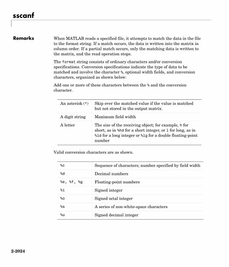
sscanf
2-2024
Remarks When MATLAB reads a specified file, it attempts to match the data in the file to the format string. If a match occurs, the data is written into the matrix in column order. If a partial match occurs, only the matching data is written to the matrix, and the read operation stops.
The format string consists of ordinary characters and/or conversion specifications. Conversion specifications indicate the type of data to be matched and involve the character %, optional width fields, and conversion characters, organized as shown below:
Add one or more of these characters between the % and the conversion character.
Valid conversion characters are as shown.
An asterisk (*) Skip over the matched value if the value is matched but not stored in the output matrix.
A digit string Maximum field width
A letter The size of the receiving object; for example, h for short, as in %hd for a short integer, or l for long, as in %ld for a long integer or %lg for a double floating-point number
%c Sequence of characters; number specified by field width
%d Decimal numbers
%e, %f, %g Floating-point numbers
%i Signed integer
%o Signed octal integer
%s A series of non-white-space characters
%u Signed decimal integer

sscanf
2-2025
If %s is used, an element read might use several MATLAB matrix elements, each holding one character. Use %c to read space characters, or %s to skip all white space.
Mixing character and numeric conversion specifications cause the resulting matrix to be numeric and any characters read to appear as their ASCII values, one character per MATLAB matrix element.
For more information about format strings, refer to the scanf() and fscanf() routines in a C language reference manual.
Examples Example 1The statements
s = '2.7183 3.1416';A = sscanf(s,'%f')
create a two-element vector containing poor approximations to e and pi.
Example 2
Create matrix A with both character and numeric data:
A = ['abc 46 6 ghi'; 'def 7 89 jkl'] A = abc 46 6 ghi def 7 89 jkl
Read A into 2-by-N matrix B, ignoring the character data. As stated in the Description section, sscanf fills matrix B in column order:
B = sscanf(A, '%*s %d %d %*s', [2, inf])B = 476 869
If you want sscanf to return the numeric data in B in the same order as in A, you can use this technique:
%x Signed hexadecimal integer
[...] Sequence of characters (scanlist)

sscanf
2-2026
for k = 1:2 C(k,:) = sscanf(A(k, :)', '%*s %d %d %*s', [1, inf]);end
CC = 46 6 7 89
See Also eval, sprintf, textread

stairs
2-2027
2stairsPurpose Stairstep graph
Syntax stairs(Y)stairs(X,Y)stairs(...,LineSpec)stairs(...,'PropertyName',propertyvalue)stairs(axes_handle,...)h = stairs(...)[xb,yb] = stairs(Y,...)
Description Stairstep graphs are useful for drawing time-history graphs of digitally sampled data.
stairs(Y) draws a stairstep graph of the elements of Y, drawing one line per column for matrices. The axes ColorOrder property determines the color of the lines.
When Y is a vector, the x-axis scale ranges from 1 to length(Y). When Y is a matrix, the x-axis scale ranges from 1 to the number of rows in Y.
stairs(X,Y) plots the elements in Y at the locations specified in X. The elements of X must be monotonic.
X must be the same size as Y or, if Y is a matrix, X can be a row or a column vector such that
length(X) = size(Y,1)
stairs(...,LineSpec) specifies a line style, marker symbol, and color for the graph (see LineSpec for more information).
stairs(...,'PropertyName',propertyvalue) creates the stairstep graph, applying the specified property settings. See Stairseries Properties for a description of properties.
stairs(axes_handles,...) plots into the axes with handle axes_handle instead of the current axes (gca).
h = stairs(...) returns the handles of the stairseries objects created (one per matrix column).

stairs
2-2028
[xb,yb] = stairs(Y,...) does not draw graphs, but returns vectors xb and yb such that plot(xb,yb) plots the stairstep graph.
Backward Compatible Version
hlines = stairs('v6',...) returns the handles of line objects instead of stairseries objects for compatibility with MATLAB 6.5 and earlier.
Examples Create a stairstep plot of a sine wave.
x = linspace(-2*pi,2*pi,40);stairs(x,sin(x))
See Also bar, hist, stem
“Discrete Data Plots” for related functions
See “Stairseries Properties” for property descriptions
−8 −6 −4 −2 0 2 4 6 8−1
−0.8
−0.6
−0.4
−0.2
0
0.2
0.4
0.6
0.8
1

Stairseries Properties
2-2029
2Stairseries PropertiesModifying Properties
You can set and query graphics object properties using the set and get commands or the Property Editor (propertyeditor).
Note that you cannot define default property values for stairseries objects.
See Plot Objects for information on stairseries objects.
Stairseries Property Descriptions
This section provides a description of properties. Curly braces enclose default values.
BeingDeleted on | off Read Only
This object is being deleted. The BeingDeleted property provides a mechanism that you can use to determine if objects are in the process of being deleted. MATLAB sets the BeingDeleted property to on when the object’s delete function callback is called (see the DeleteFcn property). It remains set to on while the delete function executes, after which the object no longer exists.
For example, an object’s delete function might call other functions that act on a number of different objects. These functions might not need to perform actions on objects if the objects are going to be deleted, and therefore, can check the object’s BeingDeleted property before acting.
BusyAction cancel | queue
Callback routine interruption. The BusyAction property enables you to control how MATLAB handles events that potentially interrupt executing callbacks. If there is a callback function executing, callbacks invoked subsequently always attempt to interrupt it.
If the Interruptible property of the object whose callback is executing is set to on (the default), then interruption occurs at the next point where the event queue is processed. If the Interruptible property is off, the BusyAction property (of the object owning the executing callback) determines how MATLAB handles the event. The choices are
• cancel — Discard the event that attempted to execute a second callback routine.
• queue — Queue the event that attempted to execute a second callback routine until the current callback finishes.

Stairseries Properties
2-2030
ButtonDownFcn string or function handle
Button press callback function. A callback that executes whenever you press a mouse button while the pointer is over the stairseries object.
This property can be
• A string that is a valid MATLAB expression
• The name of an M-file
• A function handle
The expression executes in the MATLAB workspace.
See Function Handle Callbacks for information on how to use function handles to define the callbacks.
Children array of graphics object handles
Children of the stairseries object. An array containing the handles of all line objects parented to the stairseries object (whether visible or not).
Note that if a child object’s HandleVisibility property is set to callback or off, its handle does not show up in the stairs Children property unless you set the Root ShowHiddenHandles property to on:
set(0,'ShowHiddenHandles','on')
Clipping on | off
Clipping mode. MATLAB clips stairs plots to the axes plot box by default. If you set Clipping to off, lines might be displayed outside the axes plot box.
Color ColorSpec
Color of lines. A three-element RGB vector or one of the MATLAB predefined names, specifying the line color. See the ColorSpec reference page for more information on specifying color.
CreateFcn string or function handle
Callback routine executed during object creation. This property defines a callback that executes when MATLAB creates a stairseries object. You must specify the callback during the creation of the object. For example,
stairs(1:10,'CreateFcn',@CallbackFcn)
where @CallbackFcn is a function handle that references the callback function.

Stairseries Properties
2-2031
MATLAB executes this routine after setting all other stairseries properties. Setting this property on an existing stairseries object has no effect.
The handle of the object whose CreateFcn is being executed is accessible only through the root CallbackObject property, which you can query using gcbo.
See Function Handle Callbacks for information on how to use function handles to define the callback function.
DeleteFcn string or function handle
Callback executed during object deletion. A callback that executes when the stairseries object is deleted (e.g., this might happen when you issue a delete command on the stairseries object, its parent axes, or the figure containing it). MATLAB executes the callback before destroying the object’s properties so the callback routine can query these values.
The handle of the object whose DeleteFcn is being executed is accessible only through the Root CallbackObject property, which can be queried using gcbo.
See Function Handle Callbacks for information on how to use function handles to define the callback function.
See the BeingDeleted property for related information.
DisplayName string
Label used by plot legends. The legend and the plot browser use this text for labels for any stairseries objects appearing in these legends.
EraseMode normal | none | xor | background
Erase mode. This property controls the technique MATLAB uses to draw and erase stairs child objects. Alternative erase modes are useful for creating animated sequences, where control of the way individual objects are redrawn is necessary to improve performance and obtain the desired effect.
• normal — Redraw the affected region of the display, performing the three-dimensional analysis necessary to ensure that all objects are rendered correctly. This mode produces the most accurate picture, but is the slowest. The other modes are faster, but do not perform a complete redraw and are therefore less accurate.
• none — Do not erase objects when they are moved or destroyed. While the objects are still visible on the screen after erasing with EraseMode none, you

Stairseries Properties
2-2032
cannot print these objects because MATLAB stores no information about their former locations.
• xor— Draw and erase the object by performing an exclusive OR (XOR) with each pixel index of the screen behind it. Erasing the object does not damage the color of the objects behind it. However, the color of the erased object depends on the color of the screen behind it and it is correctly colored only when it is over the axes background color (or the figure background color if the axes Color property is set to none). That is, it isn’t erased correctly if there are objects behind it.
• background — Erase the graphics objects by redrawing them in the axes background color, (or the figure background color if the axes Color property is set to none). This damages other graphics objects that are behind the erased object, but the erased object is always properly colored.
Printing with Nonnormal Erase ModesMATLAB always prints figures as if the EraseMode of all objects is normal. This means graphics objects created with EraseMode set to none, xor, or background can look different on screen than on paper. On screen, MATLAB can mathematically combine layers of colors (e.g., performing an XOR operation on a pixel color with that of the pixel behind it) and ignore three-dimensional sorting to obtain greater rendering speed. However, these techniques are not applied to the printed output.
Set the axes background color with the axes Color property. Set the figure background color with the figure Color property.
You can use the MATLAB getframe command or other screen capture applications to create an image of a figure containing nonnormal mode objects.
HandleVisibility on | callback | off
Control access to object’s handle by command-line users and GUIs. This property determines when an object’s handle is visible in its parent’s list of children. HandleVisibility is useful for preventing command-line users from accidentally accessing the stairseries object.
• on — Handles are always visible when HandleVisibility is on.
• callback — Setting HandleVisibility to callback causes handles to be visible from within callback routines or functions invoked by callback routines, but not from within functions invoked from the command line. This

Stairseries Properties
2-2033
provides a means to protect GUIs from command-line users, while allowing callback routines to have access to object handles.
• off — Setting HandleVisibility to off makes handles invisible at all times. This might be necessary when a callback invokes a function that might potentially damage the GUI (such as evaluating a user-typed string) and so temporarily hides its own handles during the execution of that function.
Functions Affected by Handle VisibilityWhen a handle is not visible in its parent’s list of children, it cannot be returned by functions that obtain handles by searching the object hierarchy or querying handle properties. This includes get, findobj, gca, gcf, gco, newplot, cla, clf, and close.
Properties Affected by Handle VisibilityWhen a handle’s visibility is restricted using callback or off, the object’s handle does not appear in its parent’s Children property, figures do not appear in the root’s CurrentFigure property, objects do not appear in the root’s CallbackObject property or in the figure’s CurrentObject property, and axes do not appear in their parent’s CurrentAxes property.
Overriding Handle VisibilityYou can set the root ShowHiddenHandles property to on to make all handles visible regardless of their HandleVisibility settings (this does not affect the values of the HandleVisibility properties). See also findall.
Handle ValidityHandles that are hidden are still valid. If you know an object’s handle, you can set and get its properties and pass it to any function that operates on handles.
HitTest on | off
Selectable by mouse click. HitTest determines if the stairseries object can become the current object (as returned by the gco command and the figure CurrentObject property) as a result of a mouse click on the line objects that compose the stairs plot. If HitTest is off, clicking the stairseries object selects the object below it (which is usually the axes containing it).
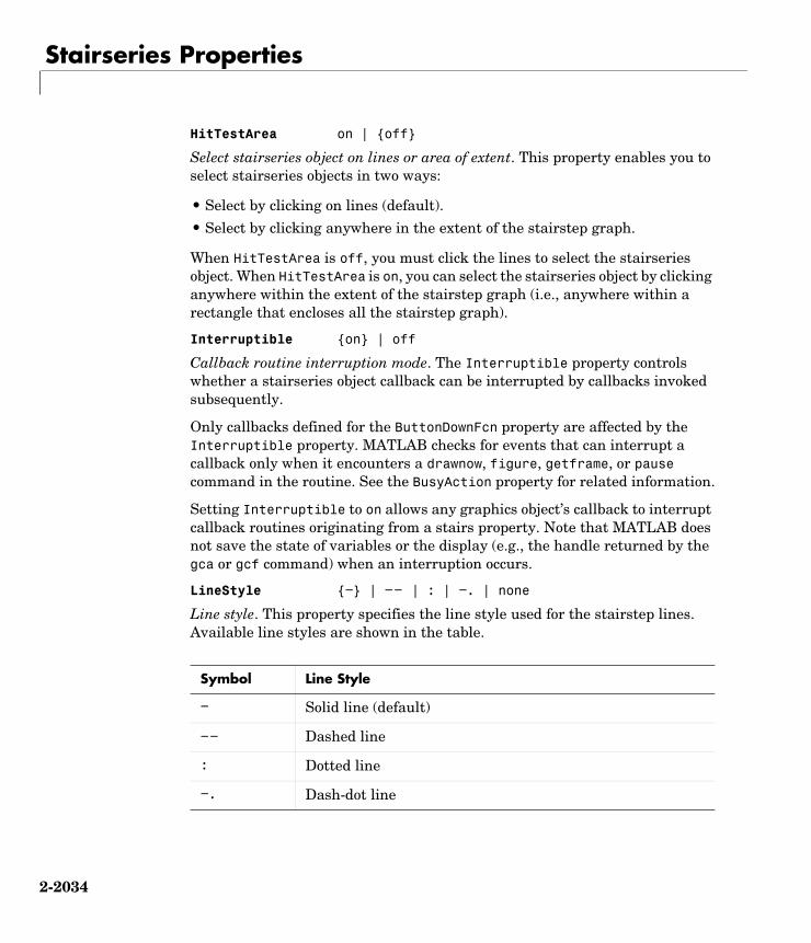
Stairseries Properties
2-2034
HitTestArea on | off
Select stairseries object on lines or area of extent. This property enables you to select stairseries objects in two ways:
• Select by clicking on lines (default).
• Select by clicking anywhere in the extent of the stairstep graph.
When HitTestArea is off, you must click the lines to select the stairseries object. When HitTestArea is on, you can select the stairseries object by clicking anywhere within the extent of the stairstep graph (i.e., anywhere within a rectangle that encloses all the stairstep graph).
Interruptible on | off
Callback routine interruption mode. The Interruptible property controls whether a stairseries object callback can be interrupted by callbacks invoked subsequently.
Only callbacks defined for the ButtonDownFcn property are affected by the Interruptible property. MATLAB checks for events that can interrupt a callback only when it encounters a drawnow, figure, getframe, or pause command in the routine. See the BusyAction property for related information.
Setting Interruptible to on allows any graphics object’s callback to interrupt callback routines originating from a stairs property. Note that MATLAB does not save the state of variables or the display (e.g., the handle returned by the gca or gcf command) when an interruption occurs.
LineStyle − | −− | : | −. | none
Line style. This property specifies the line style used for the stairstep lines. Available line styles are shown in the table.
Symbol Line Style
− Solid line (default)
−− Dashed line
: Dotted line
−. Dash-dot line

Stairseries Properties
2-2035
You can use LineStyle none when you want to place a marker at each point but do not want the points connected with a line (see the Marker property).
LineWidth scalar
The width of the stairs lines. Specify this value in points (1 point = 1/72 inch). The default LineWidth is 0.5 points.
Marker character (see table)
Marker symbol. The Marker property specifies the type of markers that are displayed at the end of the stairs lines. You can set values for the Marker property independently from the LineStyle property. Supported markers include those shown in the following table.
none No line
Marker Specifier Description
+ Plus sign
o Circle
* Asterisk
. Point
x Cross
s Square
d Diamond
^ Upward-pointing triangle
v Downward-pointing triangle
> Right-pointing triangle
< Left-pointing triangle
p Five-pointed star (pentagram)
Symbol Line Style

Stairseries Properties
2-2036
MarkerEdgeColor ColorSpec | none | auto
Marker edge color. The color of the marker or the edge color for filled markers (circle, square, diamond, pentagram, hexagram, and the four triangles). ColorSpec defines the color to use. none specifies no color, which makes nonfilled markers invisible. auto sets MarkerEdgeColor to the same color as the stairs Color property.
MarkerFaceColor ColorSpec | none | auto
Marker face color. The fill color for markers that are closed shapes (circle, square, diamond, pentagram, hexagram, and the four triangles). ColorSpec defines the color to use. none makes the interior of the marker transparent, allowing the background to show through. auto sets the fill color to the axes color, or the figure color, if the axes Color property is set to none (which is the factory default for axes).
MarkerSize size in points
Marker size. A scalar specifying the size of the marker in points. The default value for MarkerSize is 6 points (1 point = 1/72 inch). Note that MATLAB draws the point marker (specified by the '.' symbol) at one-third the specified size.
Parent handle of axes, hggroup, or hgtransform
Parent of stairseries object. This property contains the handle of the stairseries object’s parent. The parent of a stairseries object is the axes, hggroup, or hgtransform object that contains it.
See Objects That Can Contain Other Objects for more information on parenting graphics objects.
Selected on | off
Is object selected. When you set this property to on, MATLAB displays selection handles at the corners and midpoints if the SelectionHighlight property is also on (the default). You can, for example, define the ButtonDownFcn callback
h Six-pointed star (hexagram)
none No marker (default)
Marker Specifier Description

Stairseries Properties
2-2037
to set this property to on, thereby indicating that the stairseries object is selected.
SelectionHighlight on | off
Objects are highlighted when selected. When the Selected property is on, MATLAB indicates the selected state by drawing selection handles on the stairseries object. When SelectionHighlight is off, MATLAB does not draw the handles.
Tag string
User-specified object label. The Tag property provides a means to identify graphics objects with a user-specified label. This is particularly useful when you are constructing interactive graphics programs that would otherwise need to define object handles as global variables or pass them as arguments between callbacks.
For example, you might create a stairseries object and set the Tag property:
t = stairs(Y,'Tag','stairs1')
When you want to access the stairseries object, you can use findobj to find the stairseries object’s handle. The following statement changes the MarkerFaceColor property of the object whose Tag is stairs1.
set(findobj('Tag','stairs1'),'MarkerFaceColor','red')
Type string (read only)
Type of graphics object. This property contains a string that identifies the class of the graphics object. For stairseries objects, Type is 'hggroup'. The following statement finds all the hggroup objects in the current axes.
t = findobj(gca,'Type','hggroup');
UIContextMenu handle of a uicontextmenu object
Associate a context menu with the stairseries object. Assign this property the handle of a uicontextmenu object created in the stairseries object’s parent figure. Use the uicontextmenu function to create the context menu. MATLAB displays the context menu whenever you right-click over the stairseries object.

Stairseries Properties
2-2038
UserData array
User-specified data. This property can be any data you want to associate with the stairseries object (including cell arrays and structures). The stairseries object does not set values for this property, but you can access it using the set and get functions.
Visible on | off
Visibility of stairseries object and its children. By default, stairseries object visibility is on. This means all children of the stairs are visible unless the child object’s Visible property is set to off. Setting a stairseries object’s Visible property to off also makes its children invisible.
XData array
X-axis location of stairs. The stairs function uses XData to label the x-axis. XData can be either a matrix equal in size to YData or a vector equal in length to the number of rows in YData. That is, length(XData) == size(YData,1). XData must be monotonic.
If you do not specify XData (i.e., the input argument x), the stairs function uses the indices of YData to create the stairstep graph. See the XDataMode property for related information.
XDataMode auto | manual
Use automatic or user-specified x-axis values. If you specify XData (by setting the XData property or specifying the input argument x), the stairs function sets this property to manual.
If you set XDataMode to auto after having specified XData, the stairs function resets the stairs locations and x tick-mark labels to the indices of the YData, overwriting any previous values.
XDataSource string (MATLAB variable)
Link XData to MATLAB variable. Set this property to a MATLAB variable that, by default, is evaluated in the base workspace to generate the XData.
MATLAB reevaluates this property only when you set it. Therefore, a change to workspace variables appearing in an expression does not change XData.
You can use the refreshdata function to force an update of the object’s data. refreshdata also enables you to specify that the data source variable be evaluated in the workspace of a function from which you call refreshdata.

Stairseries Properties
2-2039
See the refreshdata reference page for more information.
Note If you change one data source property to return data of a different dimension, you might cause the function to generate a warning and not render the graph until you have changed all data source properties to appropriate values.
YData scalar, vector, or matrix
Stairs plot data. YData contains the data plotted in the stairstep graph. Each value in YData is represented by a marker in the stairstep graph. If YData is a matrix, the stairs function creates a line for each column in the matrix.
The input argument y in the stairs function calling syntax assigns values to YData.
YDataSource string (MATLAB variable)
Link YData to MATLAB variable. Set this property to a MATLAB variable that, by default, is evaluated in the base workspace to generate the YData.
MATLAB reevaluates this property only when you set it. Therefore, a change to workspace variables appearing in an expression does not change YData.
You can use the refreshdata function to force an update of the object’s data. refreshdata also enables you to specify that the data source variable be evaluated in the workspace of a function from which you call refreshdata.
See the refreshdata reference page for more information.
Note If you change one data source property to a variable that contains data of a different dimension, you might cause the function to generate a warning and not render the graph until you have changed all data source properties to appropriate values.
start
2-2040
2startPurpose Start timer(s) running
Syntax start(obj)
Description start(obj) starts the timer running, represented by the timer object, obj. If obj is an array of timer objects, start starts all the timers. Use the timer function to create a timer object.
start sets the Running property of the timer object, obj, to 'on', initiates TimerFcn callbacks, and executes the StartFcn callback.
The timer stops running if one of the following conditions apply:
• The number of TimerFcn callbacks specified in TasksToExecute have been executed.
• The stop(obj) command is issued.
• An error occurred while executing a TimerFcn callback.
See Also timer, stop

startat
2-2041
2startatPurpose Start timer(s) running at the specified time
Syntax startat(obj,time) startat(obj,S)startat(obj,S,pivotyear)startat(obj,Y,M,D)startat(obj,[Y,M,D])startat(obj,Y,M,D,H,MI,S)startat(obj,[Y,M,D,H,MI,S])
Description startat(obj,time) starts the timer running, represented by the timer object obj, at the time specified by the serial date number time. If obj is an array of timer objects, startat starts all the timers running at the specified time. Use the timer function to create the timer object.
startat sets the Running property of the timer object, obj, to 'on', initiates TimerFcn callbacks, and executes the StartFcn callback.
The serial date number, time, indicates the number of days that have elapsed since 1-Jan-0000 (starting at 1). See datenum for additional information about serial date numbers.
startat(obj,S) starts the timer running at the time specified by the date string S. The date string must use date format 0, 1, 2, 6, 13, 14, 15, 16, or 23, as defined by the datestr function. Date strings with two-character years are interpreted to be within the 100 years centered on the current year.
startat(obj,S,pivotyear) uses the specified pivot year as the starting year of the 100-year range in which a two-character year resides. The default pivot year is the current year minus 50 years.
startat(obj,Y,M,D)startat(obj,[Y,M,D]) start the timer at the year (Y), month (M), and day (D) specified. Y, M, and D must be arrays of the same size (or they can be a scalar).
startat(obj,Y,M,D,H,MI,S)startat(obj,[Y,M,D,H,MI,S]) start the timer at the year (Y), month (M), day (D), hour (H), minute (MI), and second (S) specified. Y, M, D, H, MI, and S must be arrays of the same size (or they can be a scalar). Values outside the normal range of each array are automatically carried to the next unit (for example,

startat
2-2042
month values greater than 12 are carried to years). Month values less than 1 are set to be 1; all other units can wrap and have valid negative values.
The timer stops running if one of the following conditions apply:
• The number of TimerFcn callbacks specified in TasksToExecute have been executed.
• The stop(obj) command is issued.
• An error occurred while executing a TimerFcn callback.
Examples This example uses a timer object to execute a function at a specified time.
t1=timer('TimerFcn','disp(''it is 10 o''''clock'')');startat(t1,'10:00:00');
This example uses a timer to display a message when an hour has elapsed.
t2=timer('TimerFcn','disp(''It has been an hour now.'')');startat(t2,now+1/24);
See Also datenum, datestr, now, timer, start, stop

startup
2-2043
2startupPurpose MATLAB startup M-file for user-defined options
Description startup automatically executes the master M-file matlabrc.m and, if it exists, startup.m, when MATLAB starts. On multiuser or networked systems, matlabrc.m is reserved for use by the system manager. The file matlabrc.m invokes the file startup.m if it exists on the MATLAB search path.
You can create a startup.m file in your own MATLAB directory. The file can include physical constants, Handle Graphics defaults, engineering conversion factors, or anything else you want predefined in your workspace.
There are other ways to predefine aspects of MATLAB. See Startup Options and About Preferences in the MATLAB documentation.
Algorithm Only matlabrc.m is actually invoked by MATLAB at startup. However, matlabrc.m contains the statements
if exist('startup')==2startup
end
that invoke startup.m. You can extend this process to create additional startup M-files, if required.
See Also matlabrc, matlabroot, path, quit

std
2-2044
2stdPurpose Standard deviation
Syntax s = std(X)s = std(X,flag)s = std(X,flag,dim)
Definition There are two common textbook definitions for the standard deviation s of a data vector X.
where
and is the number of elements in the sample. The two forms of the equation differ only in versus in the divisor.
Description s = std(X), where X is a vector, returns the standard deviation using (1) above. If X is a random sample of data from a normal distribution, is the best unbiased estimate of its variance.
If X is a matrix, std(X) returns a row vector containing the standard deviation of the elements of each column of X. If X is a multidimensional array, std(X) is the standard deviation of th elements along the first nonsingleton dimension of X.
s = std(X,flag) for flag = 0, is the same as std(X). For flag = 1, std(X,1) returns the standard deviation using (2) above, producing the second moment of the sample about its mean.
(1) s 1n 1–------------- xi x–( )2
i 1=
n
∑
12---
=
(2) s 1n--- xi x–( )2
i 1=
n
∑
12---
=
x 1n--- xi
i 1=
n
∑=
nn 1– n
s2

std
2-2045
s = std(X,flag,dim) computes the standard deviations along the dimension of X specified by scalar dim.
Examples For matrix X
X =1 5 9
7 15 22
s = std(X,0,1) s =
4.2426 7.0711 9.1924
s = std(X,0,2)s =
4.0007.5056
See Also corrcoef, cov, mean, median

stem
2-2046
2stemPurpose Plot discrete sequence data
Syntax stem(Y)stem(X,Y)stem(...,'fill')stem(...,LineSpec)stem(axes_handle,...)h = stem(...)hlines = stem('v6',...)
Description A two-dimensional stem plot displays data as lines extending from a baseline along the x-axis. A circle (the default) or other marker whose y-position represents the data value terminates each stem.
stem(Y) plots the data sequence Y as stems that extend from equally spaced and automatically generated values along the x-axis. When Y is a matrix, stem plots all elements in a row against the same x value.
stem(X,Y) plots X versus the columns of Y. X and Y must be vectors or matrices of the same size. Additionally, X can be a row or a column vector and Y a matrix with length(X) rows.
stem(...,'fill') specifies whether to color the circle at the end of the stem.
stem(...,LineSpec) specifies the line style, marker symbol, and color for the stem and top marker (the baseline is not affected). See LineSpec for more information.
stem(axes_handles,...) plots into the axes with handle axes_handle instead of the current axes (gca).
h = stem(...) returns a vector of stemseries object handles in h, one handle per column of data in Y.
Backward Compatible Version
hlines = stem('v6',...) returns the handles of line objects instead of stemseries objects for compatibility with MATLAB 6.5 and earlier.
hlines contains the handles to three line graphics objects:

stem
2-2047
• hlines(1) — The marker symbol at the top of each stem
• hlines(2) — The stem line
• hlines(3) — The baseline handle
See Plot Objects and Backward Compatibility for more information.
Examples Single Series of DataThis example creates a stem plot representing the cosine of 10 values linearly spaced between 0 and 2π. Note that the line style of the baseline is set by first getting its handle from the stemseries object’s BaseLine property.
t = linspace(-2*pi,2*pi,10);h = stem(t,cos(t),'fill','--');set(get(h,'BaseLine'),'LineStyle',':')set(h,'MarkerFaceColor','red')
−8 −6 −4 −2 0 2 4 6 8−1
−0.8
−0.6
−0.4
−0.2
0
0.2
0.4
0.6
0.8
1

stem
2-2048
The following diagram illustrates the parent-child relationship in the previous stem plot. Note that the stemseries object contains two line objects used to draw the stem lines and the end markers. The baseline is a separate line object.
Two Series of Data on One GraphThe following example creates a stem plot from a two-column matrix. In this case, the stem function creates two stemseries objects, one of each column of data. Both objects’ handles are returned in the output argument h.
• h(1) is the handle to the stemseries object plotting the expression exp(-.07*x).*cos(x).
• h(2) is the handle to the stemseries object plotting the expression exp(.05*x).*cos(x).
x = 0:25;y = [exp(-.07*x).*cos(x);exp(.05*x).*cos(x)]';h = stem(x,y);set(h(1),'MarkerFaceColor','blue')set(h(2),'MarkerFaceColor','red','Marker','square')
Line
Stemseries
Axes
Line(stems) (markers)
Line(baseline)

stem
2-2049
The following diagram illustrates the parent-child relationship in the previous stem plot. Note that each column in the input matrix y results in the creation of a stemseries object, which contains two line objects (one for the stems and one for the markers). The baseline is shared by both stemseries objects.
0 5 10 15 20 25−4
−3
−2
−1
0
1
2
3
4
Line
Stemseries
Axes
Stemseries
Line(stems) (markers)
Line Line(stems) (markers)
Line(baseline)blue red

stem
2-2050
See Also bar, plot, stairs
See “Stemseries Properties” for property descriptions

stem3
2-2051
2stem3Purpose Plot three-dimensional discrete sequence data
Syntax stem3(Z)stem3(X,Y,Z)stem3(...,'fill')stem3(...,LineSpec)h = stem3(...)hlines = stem3('v6',...)
Description Three-dimensional stem plots display lines extending from the x-y plane. A circle (the default) or other marker symbol whose z-position represents the data value terminates each stem.
stem3(Z) plots the data sequence Z as stems that extend from the x-y plane. x and y are generated automatically. When Z is a row vector, stem3 plots all elements at equally spaced x values against the same y value. When Z is a column vector, stem3 plots all elements at equally spaced y values against the same x value.
stem3(X,Y,Z) plots the data sequence Z at values specified by X and Y. X, Y, and Z must all be vectors or matrices of the same size.
stem3(...,'fill') specifies whether to color the interior of the circle at the end of the stem.
stem3(...,LineSpec) specifies the line style, marker symbol, and color for the stems. See LineSpec for more information.
h = stem3(...) returns handles to stemseries graphics objects.
Backward Compatible Version
hlines = stem3('v6',...) returns the handles of line objects instead of stemseries objects for compatibility with MATLAB 6.5 and earlier.
Examples Create a three-dimensional stem plot to visualize a function of two variables.
X = linspace(0,1,10);Y = X./2;Z = sin(X) + cos(Y);

stem3
2-2052
stem3(X,Y,Z,'fill')view(-25,30)
:
See Also bar, plot, stairs, stem
“Discrete Data Plots” for related functions
“Stemseries Properties” for descriptions of properties.
Three-Dimensional Stem Plots for more examples.
00.2
0.40.6
0.81
00.1
0.20.3
0.40.5
0
0.5
1
1.5
2

Stemseries Properties
2-2053
2Stemseries PropertiesModifying Properties
You can set and query graphics object properties using the set and get commands or with the property editor (propertyeditor).
Note that you cannot define default properties for stemseries objects.
See Plot Objects for information on stemseries objects.
Stemseries Property Descriptions
This section provides a description of properties. Curly braces enclose default values.
BaseLine handle of baseline
Handle of the baseline object. This property contains the handle of the line object used as the baseline. You can set the properties of this line using its handle. For example, the following statements create a stem plot, obtain the handle of the baseline from the stemseries object, and then set line properties that make the baseline a dashed, red line.
stem_handle = stem(randn(10,1));baseline_handle = get(stem_handle,'BaseLine');set(baseline_handle,'LineStyle','--','Color','red')
BaseValue y-axis value
Y-axis value where baseline is drawn. You can specify the value along the y-axis at which MATLAB draws the baseline.
BeingDeleted on | off Read Only
This object is being deleted. The BeingDeleted property provides a mechanism that you can use to determine if objects are in the process of being deleted. MATLAB sets the BeingDeleted property to on when the object’s delete function callback is called (see the DeleteFcn property). It remains set to on while the delete function executes, after which the object no longer exists.
For example, an object’s delete function might call other functions that act on a number of different objects. These functions might not need to perform actions on objects if the objects are going to be deleted, and therefore can check the object’s BeingDeleted property before acting.
BusyAction cancel | queue
Callback routine interruption. The BusyAction property enables you to control how MATLAB handles events that potentially interrupt executing callbacks. If
Stemseries Properties
2-2054
there is a callback function executing, callbacks invoked subsequently always attempt to interrupt it.
If the Interruptible property of the object whose callback is executing is set to on (the default), then interruption occurs at the next point where the event queue is processed. If the Interruptible property is off, the BusyAction property (of the object owning the executing callback) determines how MATLAB handles the event. The choices are
• cancel — Discard the event that attempted to execute a second callback routine.
• queue — Queue the event that attempted to execute a second callback routine until the current callback finishes.
ButtonDownFcn string or function handle
Button press callback function. A callback that executes whenever you press a mouse button while the pointer is over the stemseries object.
This property can be
• A string that is a valid MATLAB expression
• The name of an M-file
• A function handle
The expression executes in the MATLAB workspace.
See Function Handle Callbacks for information on how to use function handles to define the callbacks.
Children array of graphics object handles
Children of the stemseries object. An array containing the handles of all line objects parented to the stemseries object (whether visible or not).
Note that if a child object’s HandleVisibility property is set to callback or off, its handle does not show up in the stem Children property unless you set the Root ShowHiddenHandles property to on:
set(0,'ShowHiddenHandles','on')
Stemseries Properties
2-2055
Clipping on | off
Clipping mode. MATLAB clips stem plots to the axes plot box by default. If you set Clipping to off, lines might be displayed outside the axes plot box.
Color ColorSpec
Color of stem lines. A three-element RGB vector or one of the MATLAB predefined names, specifying the line color. See the ColorSpec reference page for more information on specifying color.
For example, the following statement would produce a stem plot with red lines.
h = stem(randn(10,1),'Color','r');
CreateFcn string or function handle
Callback routine executed during object creation. This property defines a callback that executes when MATLAB creates a stemseries object. You must specify the callback during the creation of the object. For example,
stem(x,y,'CreateFcn',@CallbackFcn)
where @CallbackFcn is a function handle that references the callback function.
MATLAB executes this routine after setting all other stemseries properties. Setting this property on an existing stemseries object has no effect.
The handle of the object whose CreateFcn is being executed is accessible only through the root CallbackObject property, which you can query using gcbo.
See Function Handle Callbacks for information on how to use function handles to define the callback function.
DeleteFcn string or function handle
Callback executed during object deletion. A callback that executes when the stemseries object is deleted (e.g., this might happen when you issue a delete command on the stemseries object, its parent axes, or the figure containing it). MATLAB executes the callback before destroying the object’s properties so the callback routine can query these values.
The handle of the object whose DeleteFcn is being executed is accessible only through the root CallbackObject property, which can be queried using gcbo.
See Function Handle Callbacks for information on how to use function handles to define the callback function.

Stemseries Properties
2-2056
See the BeingDeleted property for related information.
DisplayName string
Label used by plot legends. The legend and the plot browser use this text for labels for any stemseries objects appearing in these legends.
EraseMode normal | none | xor | background
Erase mode. This property controls the technique MATLAB uses to draw and erase stem child objects (the lines used to construct the stem plot). Alternative erase modes are useful for creating animated sequences, where control of the way individual objects are redrawn is necessary to improve performance and obtain the desired effect.
• normal — Redraw the affected region of the display, performing the three-dimensional analysis necessary to ensure that all objects are rendered correctly. This mode produces the most accurate picture, but is the slowest. The other modes are faster, but do not perform a complete redraw and are therefore less accurate.
• none — Do not erase objects when they are moved or destroyed. While the objects are still visible on the screen after erasing with EraseMode none, you cannot print these objects because MATLAB stores no information about their former locations.
• xor— Draw and erase the object by performing an exclusive OR (XOR) with each pixel index of the screen behind it. Erasing the object does not damage the color of the objects behind it. However, the color of the erased object depends on the color of the screen behind it and it is correctly colored only when it is over the axes background color (or the figure background color if the axes Color property is set to none). That is, it isn’t erased correctly if there are objects behind it.
• background — Erase the graphics objects by redrawing them in the axes background color (or the figure background color if the axes Color property is set to none). This damages other graphics objects that are behind the erased object, but the erased object is always properly colored.
Printing with Nonnormal Erase ModesMATLAB always prints figures as if the EraseMode of all objects is normal. This means graphics objects created with EraseMode set to none, xor, or background can look different on screen than on paper. On screen, MATLAB can

Stemseries Properties
2-2057
mathematically combine layers of colors (e.g., performing an XOR operation on a pixel color with that of the pixel behind it) and ignore three-dimensional sorting to obtain greater rendering speed. However, these techniques are not applied to the printed output.
Set the axes background color with the axes Color property. Set the figure background color with the figure Color property.
You can use the MATLAB getframe command or other screen capture applications to create an image of a figure containing nonnormal mode objects.
HandleVisibility on | callback | off
Control access to object’s handle by command-line users and GUIs. This property determines when an object’s handle is visible in its parent’s list of children. HandleVisibility is useful for preventing command-line users from accidentally accessing the stemseries object.
• on — Handles are always visible when HandleVisibility is on.
• callback — Setting HandleVisibility to callback causes handles to be visible from within callback routines or functions invoked by callback routines, but not from within functions invoked from the command line. This provides a means to protect GUIs from command-line users, while allowing callback routines to have access to object handles.
• off — Setting HandleVisibility to off makes handles invisible at all times. This might be necessary when a callback invokes a function that might potentially damage the GUI (such as evaluating a user-typed string) and so temporarily hides its own handles during the execution of that function.
Functions Affected by Handle VisibilityWhen a handle is not visible in its parent’s list of children, it cannot be returned by functions that obtain handles by searching the object hierarchy or querying handle properties. This includes get, findobj, gca, gcf, gco, newplot, cla, clf, and close.
Properties Affected by Handle VisibilityWhen a handle’s visibility is restricted using callback or off, the object’s handle does not appear in its parent’s Children property, figures do not appear in the root’s CurrentFigure property, objects do not appear in the root’s

Stemseries Properties
2-2058
CallbackObject property or in the figure’s CurrentObject property, and axes do not appear in their parent’s CurrentAxes property.
Overriding Handle VisibilityYou can set the root ShowHiddenHandles property to on to make all handles visible regardless of their HandleVisibility settings (this does not affect the values of the HandleVisibility properties). See also findall.
Handle ValidityHandles that are hidden are still valid. If you know an object’s handle, you can set and get its properties and pass it to any function that operates on handles.
HitTest on | off
Selectable by mouse click. HitTest determines whether the stemseries object can become the current object (as returned by the gco command and the figure CurrentObject property) as a result of a mouse click on the line objects that compose the stem plot. If HitTest is off, clicking the stemseries object selects the object below it (which is usually the axes containing it).
HitTestArea on | off
Select stemseries object on stem lines or area of extent. This property enables you to select stemseries objects in two ways:
• Select by clicking stem lines (default).
• Select by clicking anywhere in the extent of the stem graph.
When HitTestArea is off, you must click the stem lines (excluding the baseline) to select the stemseries object. When HitTestArea is on, you can select the stemseries object by clicking anywhere within the extent of the stem plot (i.e., anywhere within a rectangle that encloses all the stem lines).
Interruptible on | off
Callback routine interruption mode. The Interruptible property controls whether a stemseries object callback can be interrupted by callbacks invoked subsequently.
Only callbacks defined for the ButtonDownFcn property are affected by the Interruptible property. MATLAB checks for events that can interrupt a callback only when it encounters a drawnow, figure, getframe, or pause command in the routine. See the BusyAction property for related information.

Stemseries Properties
2-2059
Setting Interruptible to on allows any graphics object’s callback to interrupt callback routines originating from a stem property. Note that MATLAB does not save the state of variables or the display (e.g., the handle returned by the gca or gcf command) when an interruption occurs.
LineStyle − | −− | : | −. | none
Line style. This property specifies the line style used for the stem lines. Available line styles are shown in the table.
You can use LineStyle none when you want to place a marker at each point but do not want the points connected with a line (see the Marker property).
LineWidth scalar
Width of the stem lines. Specify this value in points (1 point = 1/72 inch). The default LineWidth is 0.5 points.
Marker character (see table)
Marker symbol. The Marker property specifies the type of markers that are displayed at the end of the stem lines. You can set values for the Marker property independently from the LineStyle property. Supported markers include those shown in the following table.
Symbol Line Style
− Solid line (default)
−− Dashed line
: Dotted line
−. Dash-dot line
none No line
Marker Specifier Description
+ Plus sign
o Circle

Stemseries Properties
2-2060
MarkerEdgeColor ColorSpec | none | auto
Marker edge color. The color of the marker or the edge color for filled markers (circle, square, diamond, pentagram, hexagram, and the four triangles). ColorSpec defines the color to use. none specifies no color, which makes nonfilled markers invisible. auto sets MarkerEdgeColor to the same color as the stem Color property.
MarkerFaceColor ColorSpec | none | auto
Marker face color. The fill color for markers that are closed shapes (circle, square, diamond, pentagram, hexagram, and the four triangles). ColorSpec defines the color to use. none makes the interior of the marker transparent, allowing the background to show through. auto sets the fill color to the axes color, or the figure color, if the axes Color property is set to none (which is the factory default for axes).
* Asterisk
. Point
x Cross
s Square
d Diamond
^ Upward-pointing triangle
v Downward-pointing triangle
> Right-pointing triangle
< Left-pointing triangle
p Five-pointed star (pentagram)
h Six-pointed star (hexagram)
none No marker (default)
Marker Specifier Description
Stemseries Properties
2-2061
MarkerSize size in points
Marker size. A scalar specifying the size of the marker in points. The default value for MarkerSize is 6 points (1 point = 1/72 inch). Note that MATLAB draws the point marker (specified by the '.' symbol) at one-third the specified size.
Parent handle of axes, hggroup, or hgtransform
Parent of stemseries object. This property contains the handle of the stemseries object’s parent. The parent of a stemseries object is the axes, hggroup, or hgtransform object that contains it.
See Objects That Can Contain Other Objects for more information on parenting graphics objects.
Selected on | off
Is object selected? When you set this property to on, MATLAB displays selection handles at the corners and midpoints if the SelectionHighlight property is also on (the default). You can, for example, define the ButtonDownFcn callback to set this property to on, thereby indicating that the stemseries object has been selected.
SelectionHighlight on | off
Objects are highlighted when selected. When the Selected property is on, MATLAB indicates the selected state by drawing selection handles on the stems. When SelectionHighlight is off, MATLAB does not draw the handles.
ShowBaseLine on | off
Turn baseline display on or off. This property determines whether stem plots display a baseline from which the stems are drawn. By default, the baseline is displayed.
Tag string
User-specified object label. The Tag property provides a means to identify graphics objects with a user-specified label. This is particularly useful when you are constructing interactive graphics programs that would otherwise need to define object handles as global variables or pass them as arguments between callbacks.
For example, you might create a stemseries object and set the Tag property:
t = stem(Y,'Tag','stem1')

Stemseries Properties
2-2062
When you want to access the stemseries object, you can use findobj to find the stemseries object’s handle. The following statement changes the MarkerFaceColor property of the object whose Tag is stem1.
set(findobj('Tag','stem1'),'MarkerFaceColor','red')
Type string (read only)
Type of graphics object. This property contains a string that identifies the class of the graphics object. For stemseries objects, Type is 'hggroup'. The following statement finds all the hggroup objects in the current axes.
t = findobj(gca,'Type','hggroup');
UIContextMenu handle of a uicontextmenu object
Associate a context menu with the stemseries object. Assign this property the handle of a uicontextmenu object created in the stemseries object’s parent figure. Use the uicontextmenu function to create the context menu. MATLAB displays the context menu whenever you right-click over the stemseries object.
UserData array
User-specified data. This property can be any data you want to associate with the stemseries object (including cell arrays and structures). The stemseries object does not set values for this property, but you can access it using the set and get functions.
Visible on | off
Visibility of stemseries object and its children. By default, stemseries object visibility is on. This means all children of the stem are visible unless the child object’s Visible property is set to off. Setting a stemseries object’s Visible property to off also makes its children invisible.
XData array
X-axis location of stems. The stem function draws an individual stem at each x-axis location in the XData array. XData can be either a matrix equal in size to YData or a vector equal in length to the number of rows in YData. That is, length(XData) == size(YData,1). XData does not need to be monotonically increasing.
If you do not specify XData (i.e., the input argument x), the stem function uses the indices of YData to create the stem plot. See the XDataMode property for related information.

Stemseries Properties
2-2063
XDataMode auto | manual
Use automatic or user-specified x-axis values. If you specify XData, MATLAB sets this property to manual.
If you set XDataMode to auto after having specified XData, MATLAB resets the x-axis ticks and x-tick labels to the column indices of the ZData, overwriting any previous values for XData.
XDataSource string (MATLAB variable)
Link XData to MATLAB variable. Set this property to a MATLAB variable that, by default, is evaluated in the base workspace to generate the XData.
MATLAB reevaluates this property only when you set it. Therefore, a change to workspace variables appearing in an expression does not change XData.
You can use the refreshdata function to force an update of the object’s data. refreshdata also enables you to specify that the data source variable be evaluated in the workspace of a function from which you call refreshdata.
See the refreshdata reference page for more information.
Note If you change one data source property to return data of a different dimension, you might cause the function to generate a warning and not render the graph until you have changed all data source properties to appropriate values.
YData scalar, vector, or matrix
Stem plot data. YData contains the data plotted as stems. Each value in YData is represented by a marker in the stem plot. If YData is a matrix, MATLAB creates a series of stems for each column in the matrix.
The input argument y in the stem function calling syntax assigns values to YData.
YDataSource string (MATLAB variable)
Link YData to MATLAB variable. Set this property to a MATLAB variable that, by default, is evaluated in the base workspace to generate the YData.
MATLAB reevaluates this property only when you set it. Therefore, a change to workspace variables appearing in an expression does not change YData.

Stemseries Properties
2-2064
You can use the refreshdata function to force an update of the object’s data. refreshdata also enables you to specify that the data source variable be evaluated in the workspace of a function from which you call refreshdata.
See the refreshdata reference page for more information.
Note If you change one data source property to a variable that contains data of a different dimension, you might cause the function to generate a warning and not render the graph until you have changed all data source properties to appropriate values.
ZData vector of coordinates
Z-coordinates. A data defining the stems for 3-D stem graphs. XData and YData (if specified) must be the same size.
ZDataSource string (MATLAB variable)
Link ZData to MATLAB variable. Set this property to a MATLAB variable that, by default, is evaluated in the base workspace to generate the ZData.
MATLAB reevaluates this property only when you set it. Therefore, a change to workspace variables appearing in an expression does not change ZData.
You can use the refreshdata function to force an update of the object’s data. refreshdata also enables you to specify that the data source variable be evaluated in the workspace of a function from which you call refreshdata.
See the refreshdata reference page for more information.
Note If you change one data source property to a variable that contains data of a different dimension, you might cause the function to generate a warning and not render the graph until you have changed all data source properties to appropriate values.

stop
2-2065
2stopPurpose Stop timer(s)
Syntax stop(obj)
Description stop(obj) stops the timer, represented by the timer object, obj. If obj is an array of timer objects, the stop function stops them all. Use the timer function to create a timer object.
The stop function sets the Running property of the timer object, obj, to 'off', halts further TimerFcn callbacks, and executes the StopFcn callback.
See Also timer, start

str2double
2-2066
2str2doublePurpose Convert string to double-precision value
Syntax x = str2double('str')X = str2double(C)
Description X = str2double('str') converts the string str, which should be an ASCII character representation of a real or complex scalar value, to the MATLAB double-precision representation. The string can contain digits, a comma (thousands separator), a decimal point, a leading + or - sign, an e preceding a power of 10 scale factor, and an i for a complex unit.
If str does not represent a valid scalar value, str2double returns NaN.
X = str2double(C) converts the strings in the cell array of strings C to double precision. The matrix X returned will be the same size as C.
Examples Here are some valid str2double conversions.
str2double('123.45e7')str2double('123 + 45i')str2double('3.14159')str2double('2.7i - 3.14')str2double('2.71' '3.1415')str2double('1,200.34')
See Also char, hex2num, num2str, str2num

str2func
2-2067
2str2funcPurpose Construct a function handle from a function name string
Syntax fhandle = str2func('str')
Description str2func('str') constructs a function handle fhandle for the function named in the string 'str'.
You can create a function handle using either the @function syntax or the str2func command. You can also perform this operation on a cell array of strings. In this case, an array of function handles is returned.
Examples Example 1To convert the string, 'sin', into a handle for that function, type
fh = str2func('sin')fh = @sin
Example 2If you pass a function name string in a variable, the function that receives the variable can convert the function name to a function handle using str2func. The example below passes the variable, funcname, to function makeHandle, which then creates a function handle. Here is the function M-file:
function fh = makeHandle(funcname)fh = str2func(funcname);
This is the code that calls makdHandle to construct the function handle:
makeHandle('sin')ans = @sin
Example 3In the following example, the myminbnd function expects to receive either a function handle or string in the first argument. If you pass a string, myminbnd constructs a function handle from it using str2func, and then uses that handle in a call to fminbnd:
function myminbnd(fhandle, lower, upper)if ischar(fhandle)

str2func
2-2068
disp 'converting function string to function handle ...' fhandle = str2func(fhandle);endfminbnd(fhandle, lower, upper)
Whether you call myminbnd with a function handle or function name string, the function can handle the argument appropriately:
myminbnd('humps', 0.3, 1)converting function string to function handle ...ans = 0.6370
See Also function_handle, func2str, functions

str2mat
2-2069
2str2matPurpose Form a blank padded character matrix from strings
Syntax S = str2mat(T1, T2, T3, ...)
Description S = str2mat(T1, T2, T3, ...) forms the matrix S containing the text strings T1, T2, T3, ... as rows. The function automatically pads each string with blanks in order to form a valid matrix. Each text parameter, Ti, can itself be a string matrix. This allows the creation of arbitrarily large string matrices. Empty strings are significant.
Note This routine will become obsolete in a future version. Use char instead.
Remarks str2mat differs from strvcat in that empty strings produce blank rows in the output. In strvcat, empty strings are ignored.
Examples x = str2mat('36842', '39751', '38453', '90307');
whos x Name Size Bytes Class
x 4x5 40 char array
x(2,3)
ans =
7
See Also char, strvcat

str2num
2-2070
2str2numPurpose String to number conversion
Syntax x = str2num('str')
Description x = str2num('str') converts the string str, which is an ASCII character representation of a numeric value, to numeric representation. The string can contain
• Digits
• A decimal point
• A leading + or - sign
• A letter e or d preceding a power of 10 scale factor
• A letter i or j indicating a complex or imaginary number.
The str2num function can also convert string matrices.
Examples str2num('3.14159e0') is approximately π.
To convert a string matrix,
str2num(['1 2';'3 4'])
ans =
1 2 3 4
See Also num2str, hex2num, sscanf, sparse, special characters

strcat
2-2071
2strcatPurpose String concatenation
Syntax t = strcat(s1, s2, s3, ...)
Description t = strcat(s1, s2, s3, ...) horizontally concatenates corresponding rows of the character arrays s1, s2, s3, etc. All input arrays must have the same number of rows (or any can be a single string). When the inputs are all character arrays, the output is also a character array.
When any of the inputs is a cell array of strings, strcat returns a cell array of strings formed by concatenating corresponding elements of s1, s2, etc. The inputs must all have the same size (or any can be a scalar). Any of the inputs can also be character arrays.
Trailing spaces in character array inputs are ignored and do not appear in the output. This is not true for inputs that are cell arrays of strings. Use the concatenation syntax [s1 s2 s3 ...] to preserve trailing spaces.
Remarks strcat and matrix operation are different for strings that contain trailing spaces:
a = 'hello 'b = 'goodbye'strcat(a, b)ans =hellogoodbye[a b]ans =hello goodbye
Examples Given two 1-by-2 cell arrays a and b,
a = b = 'abcde' 'fghi' 'jkl' 'mn'
the command t = strcat(a,b) yields
t = 'abcdejkl' 'fghimn'
Given the 1-by-1 cell array c = Q', the command t = strcat(a,b,c) yields

strcat
2-2072
t = 'abcdejklQ' 'fghimnQ'
See Also strvcat, cat, cellstr

strcmp
2-2073
2strcmpPurpose Compare strings
Syntax k = strcmp('str1', 'str2')TF = strcmp(S, T)
Description k = strcmp('str1', 'str2') compares the strings str1 and str2 and returns logical true (1) if the two are identical and logical false (0) otherwise.
TF = strcmp(S, T) where either S or T is a cell array of strings, returns an array TF the same size as S and T containing 1 for those elements of S and T that match and 0 otherwise. S and T must be the same size (or one can be a scalar cell). Either one can also be a character array with the right number of rows.
Remarks Note that the value returned by strcmp is not the same as the C language convention. In addition, the strcmp function is case sensitive; any leading and trailing blanks in either of the strings are explicitly included in the comparison.
strcmp is intended for comparison of character data. When used to compare numeric data, strcmp returns 0.
Examples strcmp('Yes', 'No') =0
strcmp('Yes', 'Yes') =1
A = 'MATLAB' 'SIMULINK'
'Toolboxes' 'The MathWorks'
B = 'Handle Graphics' 'Real Time Workshop'
'Toolboxes' 'The MathWorks'
C = 'Signal Processing' 'Image Processing'
'MATLAB' 'SIMULINK'
strcmp(A, B)ans =
0 0 1 1

strcmp
2-2074
strcmp(A, C)ans =
0 0 0 0
See Also strcmpi, strncmp, strncmpi, strmatch, strfind, findstr, regexp, regexpi, regexprep

strcmpi
2-2075
2strcmpiPurpose Compare strings ignoring case
Syntax strcmpi(str1, str2)strcmpi(S, T)
Description strcmpi(str1, str2) returns 1 if strings str1 and str2 are the same except for case and 0 otherwise.
strcmpi(S, T) when either S or T is a cell array of strings, returns an array the same size as S and T containing 1 for those elements of S and T that match except for case, and 0 otherwise. S and T must be the same size (or one can be a scalar cell). Either one can also be a character array with the right number of rows.
Remarks strcmpi is intended for comparison of character data. When used to compare numeric data, strcmpi returns 0.
strcmpi supports international character sets.
See Also strcmp, strncmpi, strncmp, strmatch, strfind, findstr, regexp, regexpi, regexprep

stream2
2-2076
2stream2Purpose Compute 2-D streamline data
Syntax XY = stream2(x,y,u,v,startx,starty)XY = stream2(u,v,startx,starty)XY = stream2(...,options)
Description XY = stream2(x,y,u,v,startx,starty) computes streamlines from vector data u and v. The arrays x and y define the coordinates for u and v and must be monotonic and 2-D plaid (such as the data produced by meshgrid). startx and starty define the starting positions of the streamlines. The section “Specifying Starting Points for Stream Plots” provides more information on defining starting points.
The returned value XY contains a cell array of vertex arrays.
XY = stream2(u,v,startx,starty) assumes the arrays x and y are defined as [x,y] = meshgrid(1:n,1:m) where [m,n] = size(u).
XY = stream2(...,options) specifies the options used when creating the streamlines. Define options as a one- or two-element vector containing the step size or the step size and the maximum number of vertices in a streamline:
[stepsize]
or
[stepsize, max_number_vertices]
If you do not specify a value, MATLAB uses the default:
• Stepsize = 0.1 (one tenth of a cell)
• Maximum number of vertices = 10000
Use the streamline command to plot the data returned by stream2.
Examples This example draws 2-D streamlines from data representing air currents over regions of North America.
load wind[sx,sy] = meshgrid(80,20:10:50);streamline(stream2(x(:,:,5),y(:,:,5),u(:,:,5),v(:,:,5),sx,sy));

stream2
2-2077
See Also coneplot, stream3, streamline
“Volume Visualization” for related functions
Specifying Starting Points for Stream Plots for related information

stream3
2-2078
2stream3Purpose Compute 3-D streamline data
Syntax XYZ = stream3(X,Y,Z,U,V,W,startx,starty,startz)XYZ = stream3(U,V,W,startx,starty,startz)
Description XYZ = stream3(X,Y,Z,U,V,W,startx,starty,startz) computes streamlines from vector data U, V, W. The arrays X, Y, Z define the coordinates for U, V, W and must be monotonic and 3-D plaid (such as the data produced by meshgrid). startx, starty, and startz define the starting positions of the streamlines. The section “Specifying Starting Points for Stream Plots” provides more information on defining starting points.
The returned value XYZ contains a cell array of vertex arrays.
XYZ = stream3(U,V,W,startx,starty,startz) assumes the arrays X, Y, and Z are defined as [X,Y,Z] = meshgrid(1:N,1:M,1:P) where [M,N,P] = size(U).
XYZ = stream3(...,options) specifies the options used when creating the streamlines. Define options as a one- or two-element vector containing the step size or the step size and the maximum number of vertices in a streamline:
[stepsize]
or
[stepsize, max_number_vertices]
If you do not specify values, MATLAB uses the default:
• Stepsize = 0.1 (one tenth of a cell)
• Maximum number of vertices = 10000
Use the streamline command to plot the data returned by stream3.
Examples This example draws 3-D streamlines from data representing air currents over regions of North America.
load wind[sx sy sz] = meshgrid(80,20:10:50,0:5:15);streamline(stream3(x,y,z,u,v,w,sx,sy,sz))view(3)

stream3
2-2079
See Also coneplot, stream2, streamline
“Volume Visualization” for related functions
Specifying Starting Points for Stream Plots for related information

streamline
2-2080
2streamlinePurpose Draw streamlines from 2-D or 3-D vector data
Syntax streamline(X,Y,Z,U,V,W,startx,starty,startz)streamline(U,V,W,startx,starty,startz)streamline(XYZ)streamline(X,Y,U,V,startx,starty)streamline(U,V,startx,starty)streamline(XY)streamline(...,options)streamline(axes_handle,...)h = streamline(...)
Description streamline(X,Y,Z,U,V,W,startx,starty,startz) draws streamlines from 3-D vector data U, V, W. The arrays X, Y, Z define the coordinates for U, V, W and must be monotonic and 3-D plaid (such as the data produced by meshgrid). startx, starty, startz define the starting positions of the streamlines. The section “Specifying Starting Points for Stream Plots” provides more information on defining starting points.
streamline(U,V,W,startx,starty,startz) assumes the arrays X, Y, and Z are defined as [X,Y,Z] = meshgrid(1:N,1:M,1:P) where [M,N,P] = size(U).
streamline(XYZ) assumes XYZ is a precomputed cell array of vertex arrays (as produced by stream3).
streamline(X,Y,U,V,startx,starty) draws streamlines from 2-D vector data U, V. The arrays X, Y define the coordinates for U, V and must be monotonic and 2-D plaid (such as the data produced by meshgrid). startx and starty define the starting positions of the streamlines. The output argument h contains a vector of line handles, one handle for each streamline.
streamline(U,V,startx,starty) assumes the arrays X and Y are defined as [X,Y] = meshgrid(1:N,1:M) where [M,N] = size(U).
streamline(XY) assumes XY is a precomputed cell array of vertex arrays (as produced by stream2).
streamline(...,options) specifies the options used when creating the streamlines. Define options as a one- or two-element vector containing the step size or the step size and the maximum number of vertices in a streamline:

streamline
2-2081
[stepsize]
or
[stepsize, max_number_vertices]
If you do not specify values, MATLAB uses the default:
• Stepsize = 0.1 (one tenth of a cell)
• Maximum number of vertices = 1000
streamline(axes_handles,...) plots into the axes with handle axes_handle instead of the current axes (gca).
h = streamline(...) returns a vector of line handles, one handle for each streamline.
Examples This example draws streamlines from data representing air currents over a region of North America. Loading the wind data set creates the variables x, y, z, u, v, and w in the MATLAB workspace.
The plane of streamlines indicates the flow of air from the west to the east (the x-direction) beginning at x = 80 (which is close to the minimum value of the x coordinates). The y- and z-coordinate starting points are multivalued and approximately span the range of these coordinates. meshgrid generates the starting positions of the streamlines.
load wind[sx,sy,sz] = meshgrid(80,20:10:50,0:5:15);h = streamline(x,y,z,u,v,w,sx,sy,sz);set(h,'Color','red')view(3)
See Also coneplot, stream2, stream3, streamparticles
“Volume Visualization” for related functions
Specifying Starting Points for Stream Plots for related information
Stream Line Plots of Vector Data for another example
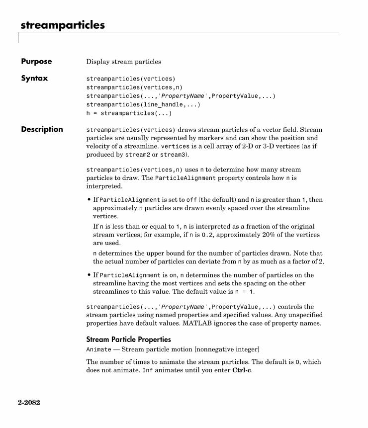
streamparticles
2-2082
2streamparticlesPurpose Display stream particles
Syntax streamparticles(vertices)streamparticles(vertices,n)streamparticles(...,'PropertyName',PropertyValue,...)streamparticles(line_handle,...)h = streamparticles(...)
Description streamparticles(vertices) draws stream particles of a vector field. Stream particles are usually represented by markers and can show the position and velocity of a streamline. vertices is a cell array of 2-D or 3-D vertices (as if produced by stream2 or stream3).
streamparticles(vertices,n) uses n to determine how many stream particles to draw. The ParticleAlignment property controls how n is interpreted.
• If ParticleAlignment is set to off (the default) and n is greater than 1, then approximately n particles are drawn evenly spaced over the streamline vertices.
If n is less than or equal to 1, n is interpreted as a fraction of the original stream vertices; for example, if n is 0.2, approximately 20% of the vertices are used.
n determines the upper bound for the number of particles drawn. Note that the actual number of particles can deviate from n by as much as a factor of 2.
• If ParticleAlignment is on, n determines the number of particles on the streamline having the most vertices and sets the spacing on the other streamlines to this value. The default value is n = 1.
streamparticles(...,'PropertyName',PropertyValue,...) controls the stream particles using named properties and specified values. Any unspecified properties have default values. MATLAB ignores the case of property names.
Stream Particle PropertiesAnimate — Stream particle motion [nonnegative integer]
The number of times to animate the stream particles. The default is 0, which does not animate. Inf animates until you enter Ctrl-c.

streamparticles
2-2083
FrameRate — Animation frames per second [nonnegative integer]
This property specifies the number of frames per second for the animation. Inf, the default, draws the animation as fast as possible. Note that the speed of the animation might be limited by the speed of the computer. In such cases, the value of FrameRate cannot necessarily be achieved.
ParticleAlignment — Align particles with streamlines [ on | off ]
Set this property to on to draw particles at the beginning of each streamline. This property controls how streamparticles interprets the argument n (number of stream particles).
Stream particles are line objects. In addition to stream particle properties, you can specify any line object property, such as Marker and EraseMode. streamparticles sets the following line properties when called.
You can override any of these properties by specifying a property name and value as arguments to streamparticles. For example, this statement uses RGB values to set the MarkerFaceColor to medium gray:
streamparticles(vertices,'MarkerFaceColor',[.5 .5 .5])
streamparticles(line_handle,...) uses the line object identified by line_handle to draw the stream particles.
h = streamparticles(...) returns a vector of handles to the line objects it creates.
Examples This example combines streamlines with stream particle animation. The interpstreamspeed function determines the vertices along the streamlines
Line Property Value Set by streamparticles
EraseMode xor
LineStyle none
Marker o
MarkerEdgeColor none
MarkerFaceColor red

streamparticles
2-2084
where stream particles will be drawn during the animation, thereby controlling the speed of the animation. Setting the axes DrawMode property to fast provides faster rendering.
load wind[sx sy sz] = meshgrid(80,20:1:55,5);verts = stream3(x,y,z,u,v,w,sx,sy,sz);sl = streamline(verts);iverts = interpstreamspeed(x,y,z,u,v,w,verts,.025);axis tight; view(30,30); daspect([1 1 .125])camproj perspective; camva(8)set(gca,'DrawMode','fast')box onstreamparticles(iverts,35,'animate',10,'ParticleAlignment','on')
The following picture is a static view of the animation.
This example uses the streamlines in the z = 5 plane to animate the flow along these lines with streamparticles.
load winddaspect([1 1 1]); view(2)[verts averts] = streamslice(x,y,z,u,v,w,[],[],[5]); sl = streamline([verts averts]);

streamparticles
2-2085
axis tight off;set(sl,'Visible','off')iverts = interpstreamspeed(x,y,z,u,v,w,verts,.05);set(gca,'DrawMode','fast','Position',[0 0 1 1],'ZLim',[4.9 5.1])set(gcf,'Color','black')streamparticles(iverts, 200, ... 'Animate',100,'FrameRate',40, ... 'MarkerSize',10,'MarkerFaceColor','yellow')
See Also interpstreamspeed, stream3, streamline
“Volume Visualization” for related functions
Creating Stream Particle Animations for more details
Specifying Starting Points for Stream Plots for related information

streamribbon
2-2086
2streamribbonPurpose Create a 3-D stream ribbon plot
Syntax streamribbon(X,Y,Z,U,V,W,startx,starty,startz)streamribbon(U,V,W,startx,starty,startz)streamribbon(vertices,X,Y,Z,cav,speed)streamribbon(vertices,cav,speed)streamribbon(vertices,twistangle)streamribbon(...,width)streamribbon(axes_handle,...)h = streamribbon(...)
Description streamribbon(X,Y,Z,U,V,W,startx,starty,startz) draws stream ribbons from vector volume data U, V, W. The arrays X, Y, Z define the coordinates for U, V, W and must be monotonic and 3-D plaid (as if produced by meshgrid). startx, starty, and startz define the starting positions of the stream ribbons at the center of the ribbons. The section “Specifying Starting Points for Stream Plots” provides more information on defining starting points.
The twist of the ribbons is proportional to the curl of the vector field. The width of the ribbons is calculated automatically.
Generally, you should set the DataAspectRatio (daspect) before calling streamribbon.
streamribbon(U,V,W,startx,starty,startz) assumes X, Y, and Z are determined by the expression
[X,Y,Z] = meshgrid(1:n,1:m,1:p)
where [m,n,p] = size(U).
streamribbon(vertices,X,Y,Z,cav,speed) assumes precomputed streamline vertices, curl angular velocity, and flow speed. vertices is a cell array of streamline vertices (as produced by stream3). X, Y, Z, cav, and speed are 3-D arrays.
streamribbon(vertices,cav,speed) assumes X, Y, and Z are determined by the expression
[X,Y,Z] = meshgrid(1:n,1:m,1:p)

streamribbon
2-2087
where [m,n,p] = size(cav).
streamribbon(vertices,twistangle) uses the cell array of vectors twistangle for the twist of the ribbons (in radians). The size of each corresponding element of vertices and twistangle must be equal.
streamribbon(...,width) sets the width of the ribbons to width.
streamribbon(axes_handles,...) plots into the axes with handle axes_handle instead of the current axes (gca).
h = streamribbon(...) returns a vector of handles (one per start point) to surface objects.
Examples This example uses stream ribbons to indicate the flow in the wind data set. Inputs include the coordinates, vector field components, and starting location for the stream ribbons.
load wind[sx sy sz] = meshgrid(80,20:10:50,0:5:15);daspect([1 1 1])streamribbon(x,y,z,u,v,w,sx,sy,sz);%-----Define viewing and lightingaxis tightshading interp;view(3);camlight; lighting gouraud

streamribbon
2-2088
This example uses precalculated vertex data (stream3), curl average velocity
(curl), and speed ( ). Using precalculated data enables you to use values other than those calculated from the single data source. In this case, the speed is reduced by a factor of 10 compared to the previous example.
load wind[sx sy sz] = meshgrid(80,20:10:50,0:5:15);daspect([1 1 1])verts = stream3(x,y,z,u,v,w,sx,sy,sz);cav = curl(x,y,z,u,v,w);spd = sqrt(u.^2 + v.^2 + w.^2).*.1;streamribbon(verts,x,y,z,cav,spd);%-----Define viewing and lightingaxis tightshading interpview(3)camlight; lighting gouraud
u2 v2 w2+ +

streamribbon
2-2089
This example specifies a twist angle for the stream ribbon.
t = 0:.15:15;verts = [cos(t)' sin(t)' (t/3)'];twistangle = cos(t)';daspect([1 1 1])streamribbon(verts,twistangle);%-----Define viewing and lightingaxis tightshading interp;view(3);camlight; lighting gouraud

streamribbon
2-2090
This example combines cone plots (coneplot) and stream ribbon plots in one graph.
%-----Define 3-D arrays x, y, z, u, v, wxmin = -7; xmax = 7;ymin = -7; ymax = 7; zmin = -7; zmax = 7; x = linspace(xmin,xmax,30);y = linspace(ymin,ymax,20);z = linspace(zmin,zmax,20);[x y z] = meshgrid(x,y,z);u = y; v = -x; w = 0*x+1;daspect([1 1 1]);[cx cy cz] = meshgrid(linspace(xmin,xmax,30),...
linspace(ymin,ymax,30),[-3 4]);h = coneplot(x,y,z,u,v,w,cx,cy,cz,'quiver');set(h,'color','k');%-----Plot two sets of streamribbons[sx sy sz] = meshgrid([-1 0 1],[-1 0 1],-6);streamribbon(x,y,z,u,v,w,sx,sy,sz);[sx sy sz] = meshgrid([1:6],[0],-6);streamribbon(x,y,z,u,v,w,sx,sy,sz);

streamribbon
2-2091
%-----Define viewing and lightingshading interpview(-30,10) ; axis off tightcamproj perspective; camva(66); camlookat; camdolly(0,0,.5,'fixtarget')camlight
See Also curl, streamtube, streamline, stream3
“Volume Visualization” for related functions
Displaying Curl with Stream Ribbons for another example
Specifying Starting Points for Stream Plots for related information

streamslice
2-2092
2streamslicePurpose Draws streamlines in slice planes
Syntax streamslice(X,Y,Z,U,V,W,startx,starty,startz)streamslice(U,V,W,startx,starty,startz)streamslice(X,Y,U,V)streamslice(U,V)streamslice(...,density)streamslice(...,'arrowmode')streamslice(...,'method')streamslice(axes_handle,...)h = streamslice(...)[vertices arrowvertices] = streamslice(...)
Description streamslice(X,Y,Z,U,V,W,startx,starty,startz) draws well spaced streamlines (with direction arrows) from vector data U, V, W in axis aligned x-, y-, z-planes starting at the points in the vectors startx, starty, startz. (The section “Specifying Starting Points for Stream Plots” provides more information on defining starting points.) The arrays X, Y, Z define the coordinates for U, V, W and must be monotonic and 3-D plaid (as if produced by meshgrid). U, V, W must be m-by-n-by-p volume arrays.
You should not assume that the flow is parallel to the slice plane. For example, in a stream slice at a constant z, the z component of the vector field W is ignored when you are calculating the streamlines for that plane.
Stream slices are useful for determining where to start streamlines, stream tubes, and stream ribbons. It is good practice is to set the axes DataAspectRatio to [1 1 1] when using streamslice.
streamslice(U,V,W,startx,starty,startz) assumes X, Y, and Z are determined by the expression
[X,Y,Z] = meshgrid(1:n,1:m,1:p)
where [m,n,p] = size(U).
streamslice(X,Y,U,V) draws well spaced streamlines (with direction arrows) from vector volume data U, V. The arrays X, Y define the coordinates for U, V and must be monotonic and 2-D plaid (as if produced by meshgrid).

streamslice
2-2093
streamslice(U,V) assumes X, Y, and Z are determined by the expression
[X,Y,Z] = meshgrid(1:n,1:m,1:p)
where [m,n,p] = size(U).
streamslice(...,density) modifies the automatic spacing of the streamlines. density must be greater than 0. The default value is 1; higher values produce more streamlines on each plane. For example, 2 produces approximately twice as many streamlines, while 0.5 produces approximately half as many.
streamslice(...,'arrowsmode') determines if direction arrows are present or not. arrowmode can be
• arrows — Draw direction arrows on the streamlines (default).
• noarrows — Do not draw direction arrows.
streamslice(...,'method') specifies the interpolation method to use. method can be
• linear — Linear interpolation (default)
• cubic — Cubic interpolation
• nearest — Nearest-neighbor interpolation
See interp3 for more information on interpolation methods.
streamslice(axes_handles,...) plots into the axes with handle axes_handle instead of the current axes (gca).
h = streamslice(...) returns a vector of handles to the line objects created.
[vertices arrowvertices] = streamslice(...) returns two cell arrays of vertices for drawing the streamlines and the arrows. You can pass these values to any of the streamline drawing functions (streamline, streamribbon, streamtube).
Examples This example creates a stream slice in the wind data set at z = 5.
load winddaspect([1 1 1])

streamslice
2-2094
streamslice(x,y,z,u,v,w,[],[],[5])axis tight
This example uses streamslice to calculate vertex data for the streamlines and the direction arrows. This data is then used by streamline to plot the lines
and arrows. Slice planes illustrating with color the wind speed ( ) are drawn by slice in the same planes.
load winddaspect([1 1 1])[verts averts] = streamslice(u,v,w,10,10,10); streamline([verts averts])spd = sqrt(u.^2 + v.^2 + w.^2);hold on; slice(spd,10,10,10);colormap(hot)shading interpview(30,50); axis(volumebounds(spd));camlight; material([.5 1 0])
u2 v2 w2+ +

streamslice
2-2095
This example superimposes contour lines on a surface and then uses streamslice to draw lines that indicate the gradient of the surface. interp2 is used to find the points for the lines that lie on the surface.
z = peaks;surf(z)shading interphold on[c ch] = contour3(z,20); set(ch,'edgecolor','b')[u v] = gradient(z); h = streamslice(-u,-v); set(h,'color','k')for i=1:length(h);
zi = interp2(z,get(h(i),'xdata'),get(h(i),'ydata'));set(h(i),'zdata',zi);
endview(30,50); axis tight

streamslice
2-2096
See Also contourslice, slice, streamline, volumebounds
“Volume Visualization” for related functions
Specifying Starting Points for Stream Plots for related information

streamtube
2-2097
2streamtubePurpose Creates a 3-D stream tube plot
Syntax streamtube(X,Y,Z,U,V,W,startx,starty,startz)streamtube(U,V,W,startx,starty,startz)streamtube(vertices,X,Y,Z,divergence)streamtube(vertices,divergence)streamtube(vertices,width)streamtube(vertices)streamtube(...,[scale n])streamtube(axes_handle,...)h = streamtube(...)
Description streamtube(X,Y,Z,U,V,W,startx,starty,startz) draws stream tubes from vector volume data U, V, W. The arrays X, Y, Z define the coordinates for U, V, W and must be monotonic and 3-D plaid (as if produced by meshgrid). startx, starty, and startz define the starting positions of the streamlines at the center of the tubes. The section “Specifying Starting Points for Stream Plots” provides more information on defining starting points.
The width of the tubes is proportional to the normalized divergence of the vector field.
Generally, you should set the DataAspectRatio (daspect) before calling streamtube.
streamtube(U,V,W,startx,starty,startz) assumes X, Y, and Z are determined by the expression
[X,Y,Z] = meshgrid(1:n,1:m,1:p)
where [m,n,p] = size(U).
streamtube(vertices,X,Y,Z,divergence) assumes precomputed streamline vertices and divergence. vertices is a cell array of streamline vertices (as produced by stream3). X, Y, Z, and divergence are 3-D arrays.
streamtube(vertices,divergence) assumes X, Y, and Z are determined by the expression
[X,Y,Z] = meshgrid(1:n,1:m,1:p)

streamtube
2-2098
where [m,n,p] = size(divergence).
streamtube(vertices,width) specifies the width of the tubes in the cell array of vectors, width. The size of each corresponding element of vertices and width must be equal. width can also be a scalar, specifying a single value for the width of all stream tubes.
streamtube(vertices) selects the width automatically.
streamtube(...,[scale n]) scales the width of the tubes by scale. The default is scale = 1. When the stream tubes are created, using start points or divergence, specifying scale = 0 suppresses automatic scaling. n is the number of points along the circumference of the tube. The default is n = 20.
streamtube(axes_handles,...) plots into the axes with handle axes_handle instead of the current axes (gca).
h = streamtube(...z) returns a vector of handles (one per start point) to surface objects used to draw the stream tubes.
Examples This example uses stream tubes to indicate the flow in the wind data set. Inputs include the coordinates, vector field components, and starting location for the stream tubes.
load wind[sx sy sz] = meshgrid(80,20:10:50,0:5:15);daspect([1 1 1])streamtube(x,y,z,u,v,w,sx,sy,sz);%-----Define viewing and lightingview(3)axis tightshading interp;camlight; lighting gouraud

streamtube
2-2099
This example uses precalculated vertex data (stream3) and divergence (divergence).
load wind[sx sy sz] = meshgrid(80,20:10:50,0:5:15);daspect([1 1 1])verts = stream3(x,y,z,u,v,w,sx,sy,sz);div = divergence(x,y,z,u,v,w);streamtube(verts,x,y,z,-div);%-----Define viewing and lightingview(3)axis tightshading interpcamlight; lighting gouraud

streamtube
2-2100
See Also divergence, streamribbon, streamline, stream3
“Volume Visualization” for related functions
Displaying Divergence with Stream Tubes for another example
Specifying Starting Points for Stream Plots for related information

strfind
2-2101
2strfindPurpose Find one string within another
Syntax k = strfind(str, pattern)k = strfind(cellstr, pattern)
Description k = strfind(str, pattern) searches the string str for occurrences of a shorter string, pattern, and returns the starting index of each such occurrence in the double array k. If pattern is not found in str, or if pattern is longer than str, then strfind returns the empty array [].
k = strfind(cellstr, pattern) searches each string in cell array of strings cellstr for occurrences of a shorter string, pattern, and returns the starting index of each such occurrence in cell array k. If pattern is not found in a string or if pattern is longer then all strings in the cell array, then strfind returns the empty array [], for that string in the cell array.
The search performed by strfind is case sensitive. Any leading and trailing blanks in pattern or in the strings being searched are explicitly included in the comparison.
Examples Use strfind to find a two-letter pattern in string S:
S = 'Find the starting indices of the pattern string';strfind(S, 'in')ans = 2 15 19 45
strfind(S, 'In')ans = []
strfind(S, ' ')ans = 5 9 18 26 29 33 41
Use strfind on a cell array of strings:
cstr = 'How much wood would a woodchuck chuck'; 'if a woodchuck could chuck wood?';
idx = strfind(cstr, 'wood');

strfind
2-2102
idx:,:ans = 10 23ans = 6 28
This means that 'wood' occurs at indices 10 and 23 in the first string and at indices 6 and 28 in the second.
See Also findstr, strmatch, strtok, strcmp, strncmp, strcmpi, strncmpi, regexp, regexpi, regexprep
strings
2-2103
2stringsPurpose MATLAB string handling
Syntax S = 'Any Characters'S = char(X)X = double(S)
Description S = 'Any Characters' creates a character array, or string. The string is actually a vector whose components are the numeric codes for the characters (the first 127 codes are ASCII). The actual characters displayed depend on the character set encoding for a given font. The length of S is the number of characters. A quotation within the string is indicated by two quotes.
S = [S1 S2 ...] concatenates character arrays S1, S2, etc. into a new character array, S.
S = strcat(S1, S2, ...) concatenates S1, S2, etc., which can be character arrays or cell arrays of strings. When the inputs are all character arrays, the output is also a character array. When any of the inputs is a cell array of strings, strcat returns a cell array of strings.
Trailing spaces in strcat character array inputs are ignored and do not appear in the output. This is not true for strcat inputs that are cell arrays of strings. Use the S = [S1 S2 ...] concatenation syntax, shown above, to preserve trailing spaces.
S = char(X) can be used to convert an array that contains positive integers representing numeric codes into a MATLAB character array.
X = double(S) converts the string to its equivalent double-precision numeric codes.
A collection of strings can be created in either of the following two ways:
• As the rows of a character array via strvcat
• As a cell array of strings via the curly braces
You can convert between character array and cell array of strings using char and cellstr. Most string functions support both types.
ischar(S) tells if S is a string variable. iscellstr(S) tells if S is a cell array of strings.

strings
2-2104
Examples Create a simple string that includes a single quote.
msg = 'You''re right!'
msg =You're right!
Create the string name using two methods of concatenation.
name = ['Thomas' ' R. ' 'Lee']
name = strcat('Thomas',' R.',' Lee')
Create a vertical array of strings.
C = strvcat('Hello','Yes','No','Goodbye')
C =Hello Yes No Goodbye
Create a cell array of strings.
S = 'Hello' 'Yes' 'No' 'Goodbye'
S = 'Hello' 'Yes' 'No' 'Goodbye'
See Also char, cellstr, ischar, iscellstr, strvcat, sprintf, sscanf, input

strjust
2-2105
2strjustPurpose Justify a character array
Syntax T = strjust(S)T = strjust(S, 'right')T = strjust(S, 'left')T = strjust(S, 'center')
Description T = strjust(S) or T = strjust(S, 'right') returns a right-justified version of the character array S.
T = strjust(S, 'left') returns a left-justified version of S.
T = strjust(S, 'center') returns a center-justified version of S.
See Also deblank

strmatch
2-2106
2strmatchPurpose Find possible matches for a string
Syntax x = strmatch('str', STRS)x = strmatch('str', STRS, 'exact')
Description x = strmatch('str', STRS) looks through the rows of the character array or cell array of strings STRS to find strings that begin with string str, returning the matching row indices. strmatch is fastest when STRS is a character array.
x = strmatch('str', STRS, 'exact') returns only the indices of the strings in STRS matching str exactly.
Examples The statement
x = strmatch('max', strvcat('max', 'minimax', 'maximum'))
returns x = [1; 3] since rows 1 and 3 begin with 'max'. The statement
x = strmatch('max', strvcat('max', 'minimax', 'maximum'),'exact')
returns x = 1, since only row 1 matches 'max' exactly.
See Also strcmp, strcmpi, strncmp, strncmpi, strfind, findstr, strvcat, regexp, regexpi, regexprep

strncmp
2-2107
2strncmpPurpose Compare the first n characters of two strings
Syntax k = strncmp('str1', 'str2', n)TF = strncmp(S, T, n)
Description k = strncmp('str1', 'str2', n) returns logical true (1) if the first n characters of the strings str1 and str2 are the same, and returns logical false (0) otherwise. Arguments str1 and str2 can also be cell arrays of strings.
TF = strncmp(S, T, N), where either S or T is a cell array of strings, returns an array TF the same size as S and T containing 1 for those elements of S and T that match (up to n characters), and 0 otherwise. S and T must be the same size (or one can be a scalar cell). Either one can also be a character array with the right number of rows.
Remarks The command strncmp is case sensitive. Any leading and trailing blanks in either of the strings are explicitly included in the comparison.
strncmp is intended for comparison of character data. When used to compare numeric data, strncmp returns 0.
See Also strncmpi, strcmp, strcmpi, strmatch, strfind, findstr, regexp, regexpi, regexprep

strncmpi
2-2108
2strncmpiPurpose Compare first n characters of strings ignoring case
Syntax strncmpi('str1', 'str2', n)TF = strncmpi(S, T, n)
Description strncmpi('str1', 'str2', n) returns 1 if the first n characters of the strings str1 and str2 are the same except for case, and 0 otherwise.
TF = strncmpi(S, T, n), when either S or T is a cell array of strings, returns an array the same size as S and T containing 1 for those elements of S and T that match except for case (up to n characters), and 0 otherwise. S and T must be the same size (or one can be a scalar cell). Either one can also be a character array with the right number of rows.
Remarks strncmpi is intended for comparison of character data. When used to compare numeric data, strncmpi returns 0.
strncmpi supports international character sets.
See Also strncmp, strcmpi, strcmp, strmatch, strfind, findstr, regexp, regexpi, regexprep

strread
2-2109
2strreadPurpose Read formatted data from a string
Syntax A = strread('str')[A, B, ...] = strread('str')[A, B, ...] = strread('str', 'format')[A, B, ...] = strread('str', 'format', N)[A, B, ...] = strread('str', 'format', N, param, value, ...)
Description A = strread('str') reads numeric data from input string str into a 1-by-N vector A, where N equals the number of whitespace-separated numbers in str. Use this form only with strings containing numeric data. See “Example 1” below.
[A, B, ...] = strread('str') reads numeric data from the string input str into scalar output variables A, B, and so on. The number of output variables must equal the number of whitespace-separated numbers in str. Use this form only with strings containing numeric data. See “Example 2” below.
[A, B, ...] = strread('str', 'format') reads data from str into variables A, B, and so on using the specified format. The number of output variables A, B, etc. must be equal to the number of format specifiers (e.g., %s or %d) in the format argument. You can read all of the data in str to a single output variable as long as you use only one format specifier in the command. See “Example 4” and “Example 5” below.
The table “Formats for strread” lists the valid format specifiers. More information on using formats is available under “Formats” in the Remarks section below.
[A, B, ...] = strread('str', 'format', N) reads data from str reusing the format string N times, where N is an integer greater than zero. If N is -1, strread reads the entire string. When str contains only numeric data, you can set format to the empty string (''). See “Example 3” below.
[A, B, ...] = strread('str', 'format', N, param, value, ...)customizes strread using param/value pairs, as listed in the table “Parameters and Values for strread” below. When str contains only numeric data, you can set format to the empty string (''). The N argument is optional and may be omitted entirely. See “Example 7” below.

strread
2-2110
Formats for strread
Format Action Output
Literals(ordinary characters)
Ignore the matching characters. For example, in a string that has Dept followed by a number (for depart-ment number), to skip the Dept and read only the number, use 'Dept' in the format string.
None
%d Read a signed integer value. Double array
%u Read an integer value. Double array
%f Read a floating-point value. Double array
%s Read a white-space separated string. Cell array of strings
%q Read a string, which could be in dou-ble quotes.
Cell array of strings. Does not include the double quotes.
%c Read characters, including white space.
Character array
%[...] Read the longest string containing characters specified in the brackets.
Cell array of strings
%[^...] Read the longest nonempty string containing characters that are not specified in the brackets.
Cell array of strings
%*... Ignore the characters following *. See Example 8 below.
No output
%w... Read field width specified by w. The %f format supports %w.pf, where w is the field width and p is the preci-sion.

strread
2-2111
Remarks DelimitersIf your data uses a character other than a space as a delimiter, you must use the strread parameter 'delimiter' to specify the delimiter. For example, if the string str used a semicolon as a delimiter, you would use this command:
[names, types, x, y, answer] = strread(str,'%s %s %f ... %d %s','delimiter',';')
Parameters and Values for strread
param value Action
white-space \* where * can be
Treats vector of characters, *, as white space. Default is \b\r\n\t.
bfnrt\\\'' or ''%%
BackspaceForm feedNew lineCarriage returnHorizontal tabBackslashSingle quotation markPercent sign
delimiter Delimiter character
Specifies delimiter character. Default is none.
expchars Exponent characters
Default is eEdD.
bufsize Positive integer
Specifies the maximum string length, in bytes. Default is 4095.
commentstyle matlab Ignores characters after %.
commentstyle shell Ignores characters after #.
commentstyle c Ignores characters between /* and */.
commentstyle c++ Ignores characters after //.
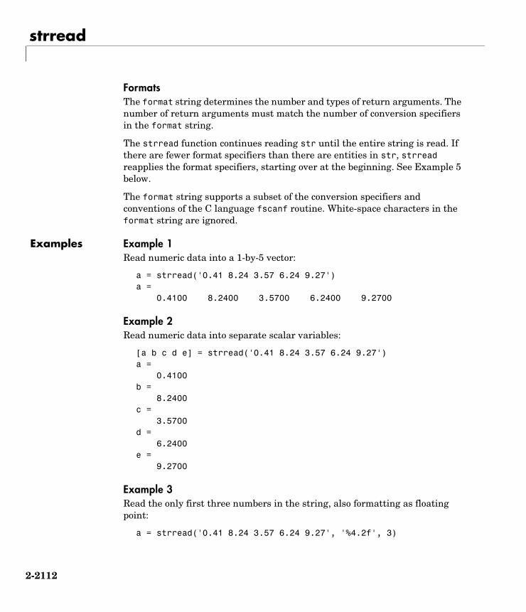
strread
2-2112
FormatsThe format string determines the number and types of return arguments. The number of return arguments must match the number of conversion specifiers in the format string.
The strread function continues reading str until the entire string is read. If there are fewer format specifiers than there are entities in str, strread reapplies the format specifiers, starting over at the beginning. See Example 5 below.
The format string supports a subset of the conversion specifiers and conventions of the C language fscanf routine. White-space characters in the format string are ignored.
Examples Example 1Read numeric data into a 1-by-5 vector:
a = strread('0.41 8.24 3.57 6.24 9.27')a = 0.4100 8.2400 3.5700 6.2400 9.2700
Example 2Read numeric data into separate scalar variables:
[a b c d e] = strread('0.41 8.24 3.57 6.24 9.27')a = 0.4100b = 8.2400c = 3.5700d = 6.2400e = 9.2700
Example 3Read the only first three numbers in the string, also formatting as floating point:
a = strread('0.41 8.24 3.57 6.24 9.27', '%4.2f', 3)

strread
2-2113
a = 0.4100 8.2400 3.5700
Example 4Truncate the data to one decimal digit by specifying format %3.1f. The second specifier, %*1d, tells strread not to read in the remaining decimal digit:
a = strread('0.41 8.24 3.57 6.24 9.27', '%3.1f %*1d')
a = 0.4000 8.2000 3.5000 6.2000 9.2000

strread
2-2114
Example 5Read six numbers into two variables, reusing the format specifiers:
[a b] = strread('0.41 8.24 3.57 6.24 9.27 3.29', '%f %f')
a = 0.4100 3.5700 9.2700b = 8.2400 6.2400 3.2900
Example 6Read string and numeric data to two output variables. Ignore commas in the input string:
str = 'Section 4, Page 7, Line 26';
[name value] = strread(str, '%s %d,')name = 'Section' 'Page' 'Line'value = 4 7 26
Example 7Read the string used in the last example, but this time delimiting with commas instead of spaces:
str = 'Section 4, Page 7, Line 26';
[a b c] = strread(str, '%s %s %s', 'delimiter', ',')

strread
2-2115
a = 'Section 4'b = 'Page 7'c = 'Line 26'
Example 8Read selected portions of the input string:
str = '<table border=5 width="100%" cellspacing=0>';
[border width space] = strread(str, ... '%*s%*s %c %*s "%4s" %*s %c', 'delimiter', '= ')border = 5width = '100%'space = 0
Example 9Read the string into two vectors, restricting the Answer values to T and F. Also note that two delimiters (comma and space) are used here:
str = 'Answer_1: T, Answer_2: F, Answer_3: F';
[a b] = strread(str, '%s %[TF]', 'delimiter', ', ')a = 'Answer_1:' 'Answer_2:' 'Answer_3:'b = 'T' 'F' 'F'
See Also textread, sscanf

strrep
2-2116
2strrepPurpose String search and replace
Syntax str = strrep(str1, str2, str3)
Description str = strrep(str1, str2, str3) replaces all occurrences of the string str2 within string str1 with the string str3.
strrep(str1, str2, str3), when any of str1, str2, or str3 is a cell array of strings, returns a cell array the same size as str1, str2, and str3 obtained by performing a strrep using corresponding elements of the inputs. The inputs must all be the same size (or any can be a scalar cell). Any one of the strings can also be a character array with the right number of rows.
Examples s1 = 'This is a good example.';str = strrep(s1, 'good', 'great')str =This is a great example.
A = 'MATLAB' 'SIMULINK'
'Toolboxes' 'The MathWorks'
B = 'Handle Graphics' 'Real Time Workshop'
'Toolboxes' 'The MathWorks'
C = 'Signal Processing' 'Image Processing'
'MATLAB' 'SIMULINK'
strrep(A, B, C)ans =
'MATLAB' 'SIMULINK' 'MATLAB' 'SIMULINK'
See Also strfind

strtok
2-2117
2strtokPurpose First token in string
Syntax token = strtok('str')token = strtok('str', delimiter)[token, rem] = strtok(...)
Description token = strtok('str') uses the default delimiters, the white-space characters. These include tabs (ASCII 9), carriage returns (ASCII 13), and spaces (ASCII 32). Any leading white-space characters are ignored. If str is a cell array of strings, token is a cell array of tokens.
token = strtok('str', delimiter) returns the first token in the text string str, that is, the first set of characters before a delimiter is encountered. The vector delimiter contains valid delimiter characters. Any leading delimiters are ignored. If str is a cell array of strings, token is a cell array of tokens.
[token, rem] = strtok(...) returns the remainder rem of the original string. The remainder consists of all characters from the first delimiter on. If str is a cell array of strings, token is a cell array of tokens, and rem is a character array.
Examples Example 1This example uses the default white-space delimiter:
s = ' This is a simple example.';[token, rem] = strtok(s)token = Thisrem = is a simple example.
Example 2Take a string of HTML code and break it down into segments delimited by the < and > characters. Write a while loop to parse the string and print each segment:

strtok
2-2118
s = sprintf('%s%s%s', ...'<ul class=continued><li class=continued><pre>', ...'<a name="13474"></a>token = strtok(''str'', delimiter)', ...'<a name="13475"></a>token = strtok(''str'')');
rem = s;
while true [tk, rem] = strtok(rem, '<>'); if isempty(tk), break; end disp(sprintf('%s',tk)) end
Here is the output:
ul class=continuedli class=continuedprea name="13474"/atoken = strtok('str', delimiter)a name="13475"/atoken = strtok('str')
Example 3Using strtok on a cell array of strings returns a cell array of strings in token and a character array in rem:
s = 'all in good time'; ... 'my dog has fleas'; ... 'leave no stone unturned';
rem = s;
for k = 1:4 [token, rem] = strtok(rem); token end

strtok
2-2119
Here is the output:
token = 'all' 'my' 'leave'token = 'in' 'dog' 'no'token = 'good' 'has' 'stone'token = 'time' 'fleas' 'unturned'
See Also findstr, strmatch

strtrim
2-2120
2strtrimPurpose Remove leading and trailing white-space from string
Syntax S = strtrim(str)C = strtrim(cstr)
Description S = strtrim(str) returns a copy of string str with all leading and trailing white-space characters removed. A white-space character is one for which the isspace function returns true.
C = strtrim(cstr) returns a copy of the cell array of strings cstr with all leading and trailing white-space characters removed from each string in the cell array.
Examples Remove the leading white-space characters (spaces and tabs) from str:
str = sprintf(' \t Remove leading white-space')str = Remove leading white-space
str = strtrim(str)str =Remove leading white-space
Remove leading and trailing white-space from the cell array of strings:
cstr = ' Trim leading white-space'; 'Trim trailing white-space ';
cstr = strtrim(cstr)cstr = 'Trim leading white-space' 'Trim trailing white-space'
See Also isspace, cellstr, deblank

struct
2-2121
2structPurpose Create structure array
Syntax s = struct('field1', , 'field2', , ...)s = struct('field1', values1, 'field2', values2, ...)
Description s = struct('field1', , 'field2', , ...) creates an empty structure with fields field1, field2, ....
s = struct('field1', values1, 'field2', values2, ...) creates a structure array with the specified fields and values. The value arrays values1, values2, etc., must be cell arrays of the same size or scalar cells. Corresponding elements of the value arrays are placed into corresponding structure array elements. The size of the resulting structure is the same size as the value cell arrays or 1-by-1 if none of the values is a cell.
Remarks The most common way to access the data in a structure is by specifying the name of the field that you want to reference. Another means of accessing structure data is to use dynamic field names. These names express the field as a variable expression that MATLAB evaluates at run-time.
Examples The command
s = struct('type', 'big','little', 'color', 'red', 'x', 3 4)
produces a structure array s:
s = 1x2 struct array with fields: type color x
The value arrays have been distributed among the fields of s:
s(1)ans =
type: 'big' color: 'red' x: 3
s(2)

struct
2-2122
ans = type: 'little'
color: 'red' x: 4
Similarly, the command
a.b = struct('z', );
produces an empty structure a.b with field z.
a.bans = 0x0 struct array with fields: z
See Also isstruct, fieldnames, isfield, orderfields, getfield, setfield, rmfield, substruct, deal, cell2struct, struct2cell, dynamic field names

struct2cell
2-2123
2struct2cellPurpose Structure to cell array conversion
Syntax c = struct2cell(s)
Description c = struct2cell(s) converts the m-by-n structure s (with p fields) into a p-by-m-by-n cell array c.
If structure s is multidimensional, cell array c has size [p size(s)].
Examples The commands
clear s, s.category = 'tree'; s.height = 37.4; s.name = 'birch';
create the structure
s = category: 'tree' height: 37.4000 name: 'birch'
Converting the structure to a cell array,
c = struct2cell(s)
c = 'tree' [37.4000] 'birch'
See Also cell2struct, cell, iscell, struct, isstruct, fieldnames, dynamic field names

strvcat
2-2124
2strvcatPurpose Vertical concatenation of strings
Syntax S = strvcat(t1, t2, t3, ...)
Description S = strvcat(t1, t2, t3, ...) forms the character array S containing the text strings (or string matrices) t1,t2,t3,... as rows. Spaces are appended to each string as necessary to form a valid matrix. Empty arguments are ignored.
Remarks If each text parameter, ti, is itself a character array, strvcat appends them vertically to create arbitrarily large string matrices.
Examples The command strvcat('Hello','Yes') is the same as ['Hello';'Yes '], except that strvcat performs the padding automatically.
t1 = 'first'; t2 = 'string'; t3 = 'matrix'; t4 = 'second';
S1 = strvcat(t1, t2, t3) S2 = strvcat(t4, t2, t3)
S1 = S2 =
first secondstring stringmatrix matrix
S3 = strvcat(S1, S2)
S3 =firststring matrixsecondstring matrix
See Also cat, int2str, mat2str, num2str, strings

sub2ind
2-2125
2sub2indPurpose Single index from subscripts
Syntax IND = sub2ind(siz,I,J)IND = sub2ind(siz,I1,I2,...,In)
Description The sub2ind command determines the equivalent single index corresponding to a set of subscript values.
IND = sub2ind(siz,I,J) returns the linear index equivalent to the row and column subscripts I and J for a matrix of size siz. siz is a 2-element vector, where siz(1) is the number of rows and siz(2) is the number of columns.
IND = sub2ind(siz,I1,I2,...,In) returns the linear index equivalent to the n subscripts I1,I2,...,In for an array of size siz. siz is an n-element vector that specifies the size of each array dimension.
Examples Create a 3-by-4-by-2 array, A.
A = [17 24 1 8; 2 22 7 14; 4 6 13 20];A(:,:,2) = A - 10
A(:,:,1) =
17 24 1 8 2 22 7 14 4 6 13 20
A(:,:,2) =
7 14 -9 -2 -8 12 -3 4 -6 -4 3 10
The value at row 2, column 1, page 2 of the array is -8.
A(2,1,2)
ans =
-8

sub2ind
2-2126
To convert A(2,1,2) into its equivalent single subscript, use sub2ind.
sub2ind(size(A),2,1,2)
ans =
14
You can now access the same location in A using the single subscripting method.
A(14)
ans =
-8
See Also ind2sub, find, size

subplot
2-2127
2subplotPurpose Create and control multiple axes
Syntax subplot(m,n,p)subplot(m,n,p,'replace')subplot(m,n,p,'align')subplot(h)subplot('Position',[left bottom width height])h = subplot(...)
Description subplot divides the current figure into rectangular panes that are numbered rowwise. Each pane contains an axes. Subsequent plots are output to the current pane.
subplot(m,n,p) creates an axes in the pth pane of a figure divided into an m-by-n matrix of rectangular panes. The new axes becomes the current axes.
If p is a vector, it specifies an axes having a position that covers all the subplot positions listed in p.
subplot(m,n,p,'replace') If the specified axes already exists, delete it and create a new axes.
subplot(m,n,p,'align') positions the individual axes so that the plot boxes align, but does not prevent the labels and ticks from overlapping.
subplot(h) makes the axes with handle h current for subsequent plotting commands.
subplot('Position',[left bottom width height]) creates an axes at the position specified by a four-element vector. left, bottom, width, and height are in normalized coordinates in the range from 0.0 to 1.0.
h = subplot(...) returns the handle to the new axes.
Remarks If a subplot specification causes a new axes to overlap any existing axes, then subplot deletes the existing axes and uicontrol objects. However, if the subplot specification exactly matches the position of an existing axes, then the matching axes is not deleted and it becomes the current axes.

subplot
2-2128
subplot(1,1,1) or clf deletes all axes objects and returns to the default subplot(1,1,1) configuration.
You can omit the parentheses and specify subplot as
subplot mnp
where m refers to the row, n refers to the column, and p specifies the pane.
Special Case – subplot(111)The command subplot(111) is not identical in behavior to subplot(1,1,1) and exists only for compatibility with previous releases. This syntax does not immediately create an axes, but instead sets up the figure so that the next graphics command executes a clf reset (deleting all figure children) and creates a new axes in the default position. This syntax does not return a handle, so it is an error to specify a return argument. (This behavior is implemented by setting the figure’s NextPlot property to replace.)
Examples To plot income in the top half of a figure and outgo in the bottom half,
income = [3.2 4.1 5.0 5.6];outgo = [2.5 4.0 3.35 4.9];subplot(2,1,1); plot(income)subplot(2,1,2); plot(outgo)

subplot
2-2129
The following illustration shows four subplot regions and indicates the command used to create each.
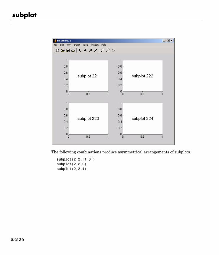
subplot
2-2130
The following combinations produce asymmetrical arrangements of subplots.
subplot(2,2,[1 3])subplot(2,2,2)subplot(2,2,4)

subplot
2-2131
You can also use the colon operator to specify multiple locations if they are in sequence.
subplot(2,2,1:2)subplot(2,2,3)subplot(2,2,4)

subplot
2-2132
See Also axes, cla, clf, figure, gca
“Basic Plots and Graphs” for more information

subsasgn
2-2133
2subsasgnPurpose Overloaded method for A(I)=B, AI=B, and A.field=B
Syntax A = subsasgn(A,S,B)
Description A = subsasgn(A,S,B) is called for the syntax A(i)=B, Ai=B, or A.i=B when A is an object. S is a structure array with the fields
• type: A string containing '()', '', or '.', where '()' specifies integer subscripts, '' specifies cell array subscripts, and '.' specifies subscripted structure fields.
• subs: A cell array or string containing the actual subscripts.
Remarks subsasgn is designed to be used by the MATLAB interpreter to handle indexed assignments to objects. Calling subsasgn directly as a function is not recommended. If you do use subsasgn in this way, it conforms to the formal MATLAB dispatching rules and can yield unexpected results.
Examples The syntax A(1:2,:)=B calls A=subsasgn(A,S,B) where S is a 1-by-1 structure with S.type='()' and S.subs = 1:2,':'. A colon used as a subscript is passed as the string ':'.
The syntax A1:2=B calls A=subsasgn(A,S,B) where S.type=''.
The syntax A.field=B calls subsasgn(A,S,B) where S.type='.' and S.subs='field'.
These simple calls are combined in a straightforward way for more complicated subscripting expressions. In such cases length(S) is the number of subscripting levels. For instance, A(1,2).name(3:5)=B calls A=subsasgn(A,S,B) where S is a 3-by-1 structure array with the following values:
See Also subsref
See “Handling Subscripted Assignment” for more information about overloaded methods and subsasgn.
S(1).type='()' S(2).type='.' S(3).type='()'
S(1).subs=1,2 S(2).subs='name' S(3).subs=3:5

subsindex
2-2134
2subsindexPurpose Overloaded method for X(A)
Syntax ind = subsindex(A)
Description ind = subsindex(A) is called for the syntax 'X(A)' when A is an object. subsindex must return the value of the object as a zero-based integer index. (ind must contain integer values in the range 0 to prod(size(X))-1.) subsindex is called by the default subsref and subsasgn functions, and you can call it if you overload these functions.
See Also subsasgn, subsref

subspace
2-2135
2subspacePurpose Angle between two subspaces
Syntax theta = subspace(A,B)
Description theta = subspace(A,B) finds the angle between two subspaces specified by the columns of A and B. If A and B are column vectors of unit length, this is the same as acos(A'*B).
Remarks If the angle between the two subspaces is small, the two spaces are nearly linearly dependent. In a physical experiment described by some observations A, and a second realization of the experiment described by B, subspace(A,B) gives a measure of the amount of new information afforded by the second experiment not associated with statistical errors of fluctuations.
Examples Consider two subspaces of a Hadamard matrix, whose columns are orthogonal.
H = hadamard(8);A = H(:,2:4);B = H(:,5:8);
Note that matrices A and B are different sizes— A has three columns and B four. It is not necessary that two subspaces be the same size in order to find the angle between them. Geometrically, this is the angle between two hyperplanes embedded in a higher dimensional space.
theta = subspace(A,B)theta = 1.5708
That A and B are orthogonal is shown by the fact that theta is equal to .
theta - pi/2ans = 0
π 2⁄

subsref
2-2136
2subsrefPurpose Overloaded method for A(I), AI and A.field
Syntax B = subsref(A,S)
Description B = subsref(A,S) is called for the syntax A(i), Ai, or A.i when A is an object. S is a structure array with the fields
• type: A string containing '()', '', or '.', where '()' specifies integer subscripts, '' specifies cell array subscripts, and '.' specifies subscripted structure fields.
• subs: A cell array or string containing the actual subscripts.
Remarks subsref is designed to be used by the MATLAB interpreter to handle indexed references to objects. Calling subsref directly as a function is not recommended. If you do use subsref in this way, it conforms to the formal MATLAB dispatching rules and can yield unexpected results.
Examples The syntax A(1:2,:) calls subsref(A,S) where S is a 1-by-1 structure with S.type='()' and S.subs=1:2,':'. A colon used as a subscript is passed as the string ':'.
The syntax A1:2 calls subsref(A,S) where S.type='' and S.subs=1:2.
The syntax A.field calls subsref(A,S) where S.type='.' and S.subs='field'.
These simple calls are combined in a straightforward way for more complicated subscripting expressions. In such cases length(S) is the number of subscripting levels. For instance, A(1,2).name(3:5) calls subsref(A,S) where S is a 3-by-1 structure array with the following values:
See Also subsasgn
See “Handling Subscripted Reference” for more information about overloaded methods and subsref.
S(1).type='()' S(2).type='.' S(3).type='()'
S(1).subs=1,2 S(2).subs='name' S(3).subs=3:5

substruct
2-2137
2substructPurpose Create structure argument for subsasgn or subsref
Syntax S = substruct(type1,subs1,type2,subs2,...)
Description S = substruct(type1,subs1,type2,subs2,...) creates a structure with the fields required by an overloaded subsref or subsasgn method. Each type string must be one of '.', '()', or ''. The corresponding subs argument must be either a field name (for the '.' type) or a cell array containing the index vectors (for the '()' or '' types).
The output S is a structure array containing the fields
• type: one of '.', '()', or ''
• subs: subscript values (field name or cell array of index vectors)
Examples To call subsref with parameters equivalent to the syntax
B = A(3,5).field
you can use
S = substruct('()',3,5,'.','field');B = subsref(A,S);
The structure created by substruct in this example contains the following:
S(1)
ans =
type: '()' subs: [3] [5]
S(2)
ans =
type: '.' subs: 'field'
See Also subsasgn, subsref

sum
2-2138
2sumPurpose Sum of array elements
Syntax B = sum(A)B = sum(A, dim)B = sum(A, 'double')B = sum(A, dim, 'double')B = sum(A, 'native')B = sum(A, dim, 'native')
Description B = sum(A) returns sums along different dimensions of an array.
If A is a vector, sum(A) returns the sum of the elements.
If A is a matrix, sum(A) treats the columns of A as vectors, returning a row vector of the sums of each column.
If A is a multidimensional array, sum(A) treats the values along the first non-singleton dimension as vectors, returning an array of row vectors.
B = sum(A,dim) sums along the dimension of A specified by scalar dim.
B = sum(..., 'double') performs additions in double-precision and return an answer of type double, even if A has data type single or an integer data type. This is the default for integer data types.
B = sum(..., 'native') performs additions in the native data type of A and return an answer of the same data type. This is the default for single and double.
Remarks sum(diag(X)) is the trace of X.
Examples The magic square of order 3 is
M = magic(3)M =
8 1 63 5 74 9 2
This is called a magic square because the sums of the elements in each column are the same.

sum
2-2139
sum(M) =15 15 15
as are the sums of the elements in each row, obtained by transposing:
sum(M') =15 15 15
Nondouble Data Type Support
This section describes the support of sum for data types other than double.
Data Type singleYou can apply sum to an array of type single and MATLAB returns an answer of type single. For example,
sum(single([2 5 8])
ans =
15
class(ans)
ans =
single
Integer Data TypesWhen you apply sum to any of the following integer data types, MATLAB returns an answer of type double:
• int8 and uint8
• int16 and uint16
• int32 and uint32
For example,
sum(single([2 5 8]);class(ans)
ans =

sum
2-2140
single
If you want MATLAB to perform additions on an integer data type in the same integer type as the input, use the syntax
sum(int8([2 5 8], 'native');class(ans)
ans =
int8
See Also cumsum, diff, prod, trac

subvolume
2-2141
2subvolumePurpose Extract subset of volume data set
Syntax [Nx,Ny,Nz,Nv] = subvolume(X,Y,Z,V,limits)[Nx,Ny,Nz,Nv] = subvolume(V,limits)Nv = subvolume(...)
Description [Nx,Ny,Nz,Nv] = subvolume(X,Y,Z,V,limits) extracts a subset of the volume data set V using the specified axis-aligned limits. limits = [xmin,xmax,ymin, ymax,zmin,zmax] (Any NaNs in the limits indicate that the volume should not be cropped along that axis.)
The arrays X, Y, and Z define the coordinates for the volume V. The subvolume is returned in NV and the coordinates of the subvolume are given in NX, NY, and NZ.
[Nx,Ny,Nz,Nv] = subvolume(V,limits) assumes the arrays X, Y, and Z are defined as
[X,Y,Z] = meshgrid(1:N,1:M,1:P)
where [M,N,P] = size(V).
Nv = subvolume(...) returns only the subvolume.
Examples This example uses a data set that is a collection of MRI slices of a human skull. The data is processed in a variety of ways:
• The 4-D array is squeezed (squeeze) into three dimensions and then a subset of the data is extracted (subvolume).
• The outline of the skull is an isosurface generated as a patch (p1) whose vertex normals are recalculated to improve the appearance when lighting is applied (patch, isosurface, isonormals).
• A second patch (p2) with interpolated face color draws the end caps (FaceColor, isocaps).
• The view of the object is set (view, axis, daspect).
• A 100-element grayscale colormap provides coloring for the end caps (colormap).
Adding lights to the right and left of the camera illuminates the object (camlight, lighting).

subvolume
2-2142
load mriD = squeeze(D);[x,y,z,D] = subvolume(D,[60,80,nan,80,nan,nan]);p1 = patch(isosurface(x,y,z,D, 5),...
'FaceColor','red','EdgeColor','none');isonormals(x,y,z,D,p1);p2 = patch(isocaps(x,y,z,D, 5),...
'FaceColor','interp','EdgeColor','none');view(3); axis tight; daspect([1,1,.4])colormap(gray(100))camlight right; camlight left; lighting gouraud
See Also isocaps, isonormals, isosurface, reducepatch, reducevolume, smooth3
“Volume Visualization” for related functions

superiorto
2-2143
2superiortoPurpose Superior class relationship
Syntax superiorto('class1','class2',...)
Description The superiorto function establishes a hierarchy that determines the order in which MATLAB calls object methods.
superiorto('class1','class2',...) invoked within a class constructor method (say myclass.m) indicates that myclass’s method should be invoked if a function is called with an object of class myclass and one or more objects of class class1, class2, and so on.
Remarks Suppose A is of class 'class_a', B is of class 'class_b' and C is of class 'class_c'. Also suppose the constructor class_c.m contains the statement superiorto('class_a'). Then e = fun(a,c) or e = fun(c,a) invokes class_c/fun.
If a function is called with two objects having an unspecified relationship, the two objects are considered to have equal precedence, and the leftmost object’s method is called. So fun(b,c) calls class_b/fun, while fun(c,b) calls class_c/fun.
See Also inferiorto

support
2-2144
2supportPurpose Open MathWorks Technical Support Web page
Syntax support
Description support opens The MathWorks Technical Support Web page, http://www.mathworks.com/support, in the MATLAB Web browser.
This Web page contains resources including
• A Search Engine, including an option for solutions to common problems
• Information about installation and licensing
• A patch archive for bug fixes you can download
• Other useful resources
See Also doc, web

surf, surfc
2-2145
2surf, surfcPurpose 3-D shaded surface plot
Syntax surf(Z)surf(X,Y,Z)surf(X,Y,Z,C)surf(...,'PropertyName',PropertyValue)surf(axes_handle,...)surfc(...)h = surf(...)h = surfc(...)hsurface = surf('v6',...), hsurface = surfc('v6',...)
Description Use surf and surfc to view mathematical functions over a rectangular region. surf and surfc create colored parametric surfaces specified by X, Y, and Z, with color specified by Z or C.
surf(Z) creates a a three-dimensional shaded surface from the z components in matrix Z, using x = 1:n and y = 1:m, where [m,n] = size(Z). The height, Z, is a single-valued function defined over a geometrically rectangular grid. Z specifies the color data as well as surface height, so color is proportional to surface height.
surf(X,Y,Z) creates a shaded surface using Z for the color data as well as surface height. X and Y are vectors or matrices defining the x and y components of a surface. If X and Y are vectors, length(X) = n and length(Y) = m, where [m,n] = size(Z). In this case, the vertices of the surface faces are
triples.
surf(X,Y,Z,C) creates a shaded surface, with color defined by C. MATLAB performs a linear transformation on this data to obtain colors from the current colormap.
surf(...,'PropertyName',PropertyValue) specifies surface properties along with the data.
surf(axes_handles,...) and surfc(axes_handles,...) plots into the axes with handle axes_handle instead of the current axes (gca).
surfc(...) draws a contour plot beneath the surface.
X j( ) Y i( ) Z i j,( ), ,( )

surf, surfc
2-2146
h = surf(...) and h = surfc(...) return a handle to a surfaceplot graphics object.
Backward Compatible Version
hsurface = surf('v6',...) and hsurface = surfc('v6',...) returns the handles of surface objects instead of surfaceplot objects for compatibility with MATLAB 6.5 and earlier.
Algorithm Abstractly, a parametric surface is parametrized by two independent variables, i and j, which vary continuously over a rectangle; for example, 1 ≤ i ≤ m and 1 ≤ j ≤ n. The three functions x(i,j), y(i,j), and z(i,j) specify the surface. When i and j are integer values, they define a rectangular grid with integer grid points. The functions x(i,j), y(i,j), and z(i,j) become three m-by-n matrices, X, Y, and Z. Surface color is a fourth function, c(i,j), denoted by matrix C.
Each point in the rectangular grid can be thought of as connected to its four nearest neighbors.
i 1,j |
i,j 1 i,j i,j+1 | i+1,j
This underlying rectangular grid induces four-sided patches on the surface. To express this another way, [X(:) Y(:) Z(:)] returns a list of triples specifying points in 3-space. Each interior point is connected to the four neighbors inherited from the matrix indexing. Points on the edge of the surface have three neighbors; the four points at the corners of the grid have only two neighbors. This defines a mesh of quadrilaterals or a quad-mesh.
Surface color can be specified in two different ways: at the vertices or at the centers of each patch. In this general setting, the surface need not be a single-valued function of x and y. Moreover, the four-sided surface patches need not be planar. For example, you can have surfaces defined in polar, cylindrical, and spherical coordinate systems.
The shading function sets the shading. If the shading is interp, C must be the same size as X, Y, and Z; it specifies the colors at the vertices. The color within

surf, surfc
2-2147
a surface patch is a bilinear function of the local coordinates. If the shading is faceted (the default) or flat, C(i,j) specifies the constant color in the surface patch:
(i,j) (i,j+1)| C(i,j) |
(i+1,j) (i+1,j+1)
In this case, C can be the same size as X, Y, and Z and its last row and column are ignored. Alternatively, its row and column dimensions can be one less than those of X, Y, and Z.
The surf and surfc functions specify the viewpoint using view(3).
The range of X, Y, and Z or the current setting of the axes XLimMode, YLimMode, and ZLimMode properties (also set by the axis function) determines the axis labels.
The range of C or the current setting of the axes CLim and ClimMode properties (also set by the caxis function) determines the color scaling. The scaled color values are used as indices into the current colormap.
Examples Display a surfaceplot and contour plot of the peaks surface.
[X,Y,Z] = peaks(30);surfc(X,Y,Z)colormap hsvaxis([−3 3 −3 3 −10 5])

surf, surfc
2-2148
Color a sphere with the pattern of +1s and -1s in a Hadamard matrix.
k = 5;n = 2^k 1;[x,y,z] = sphere(n);c = hadamard(2^k);surf(x,y,z,c);colormap([1 1 0; 0 1 1])axis equal
−3−2
−10
12
3
−3
−2
−1
0
1
2
3−10
−5
0
5

surf, surfc
2-2149
See Also axis, caxis, colormap, contour, delaunay, mesh, pcolor, shading, trisurf, view
Properties for surfaceplot graphics objects
“Creating Surfaces and Meshes” for related functions
Representing a Matrix as a Surface for more examples
Coloring Mesh and Surface Plots for information about how to control the coloring of surfaces
−1−0.5
00.5
1
−1
−0.5
0
0.5
1−1
−0.5
0
0.5
1

surf2patch
2-2150
2surf2patchPurpose Convert surface data to patch data
Syntax fvc = surf2patch(h)fvc = surf2patch(Z)fvc = surf2patch(Z,C)fvc = surf2patch(X,Y,Z)fvc = surf2patch(X,Y,Z,C)fvc = surf2patch(...,'triangles')
[f,v,c] = surf2patch(...)
Description fvc = surf2patch(h) converts the geometry and color data from the surface object identified by the handle h into patch format and returns the face, vertex, and color data in the struct fvc. You can pass this struct directly to the patch command.
fvc = surf2patch(Z) calculates the patch data from the surface’s ZData matrix Z.
fvc = surf2patch(Z,C) calculates the patch data from the surface’s ZData and CData matrices Z and C.
fvc = surf2patch(X,Y,Z) calculates the patch data from the surface’s XData, YData, and ZData matrices X, Y, and Z.
fvc = surf2patch(X,Y,Z,C) calculates the patch data from the surface’s XData, YData, ZData, and CData matrices X, Y, Z, and C.
fvc = surf2patch(...,'triangles') creates triangular faces instead of the quadrilaterals that compose surfaces.
[f,v,c] = surf2patch(...) returns the face, vertex, and color data in the three arrays f, v, and c instead of a struct.
Examples The first example uses the sphere command to generate the XData, YData, and ZData of a surface, which is then converted to a patch. Note that the ZData (z) is passed to surf2patch as both the third and fourth arguments — the third argument is the ZData and the fourth argument is taken as the CData. This is because the patch command does not automatically use the z-coordinate data for the color data, as does the surface command.

surf2patch
2-2151
Also, because patch is a low-level command, you must set the view to 3-D and shading to faceted to produce the same results produced by the surf command.
[x y z] = sphere; patch(surf2patch(x,y,z,z)); shading faceted; view(3)
In the second example surf2patch calculates face, vertex, and color data from a surface whose handle has been passed as an argument.
s = surf(peaks);pausepatch(surf2patch(s));delete(s)shading faceted; view(3)
See Also patch, reducepatch, shrinkfaces, surface, surf
“Volume Visualization” for related functions

surface
2-2152
2surfacePurpose Create surface object
Syntax surface(Z)surface(Z,C)surface(X,Y,Z)surface(X,Y,Z,C)surface(...'PropertyName',PropertyValue,...)h = surface(...)
Description surface is the low-level function for creating surface graphics objects. Surfaces are plots of matrix data created using the row and column indices of each element as the x- and y-coordinates and the value of each element as the z-coordinate.
surface(Z) plots the surface specified by the matrix Z. Here, Z is a single-valued function, defined over a geometrically rectangular grid.
surface(Z,C) plots the surface specified by Z and colors it according to the data in C (see “Examples”).
surface(X,Y,Z) uses C = Z, so color is proportional to surface height above the x-y plane.
surface(X,Y,Z,C) plots the parametric surface specified by X, Y, and Z, with color specified by C.
surface(x,y,Z), surface(x,y,Z,C) replaces the first two matrix arguments with vectors and must have length(x) = n and length(y) = m where [m,n] = size(Z). In this case, the vertices of the surface facets are the triples (x(j),y(i),Z(i,j)). Note that x corresponds to the columns of Z and y corresponds to the rows of Z. For a complete discussion of parametric surfaces, see the surf function.
surface(...'PropertyName',PropertyValue,...) follows the X, Y, Z, and C arguments with property name/property value pairs to specify additional surface properties.
h = surface(...) returns a handle to the created surface object.

surface
2-2153
Remarks surface does not respect the settings of the figure and axes NextPlot properties. It simply adds the surface object to the current axes.
If you do not specify separate color data (C), MATLAB uses the matrix (Z) to determine the coloring of the surface. In this case, color is proportional to values of Z. You can specify a separate matrix to color the surface independently of the data defining the area of the surface.
You can specify properties as property name/property value pairs, structure arrays, and cell arrays (see set and get for examples of how to specify these data types).
surface provides convenience forms that allow you to omit the property name for the XData, YData, ZData, and CData properties. For example,
surface('XData',X,'YData',Y,'ZData',Z,'CData',C)
is equivalent to
surface(X,Y,Z,C)
When you specify only a single matrix input argument,
surface(Z)
MATLAB assigns the data properties as if you specified
surface('XData',[1:size(Z,2)],...'YData',[1:size(Z,1)],...'ZData',Z,...'CData',Z)
The axis, caxis, colormap, hold, shading, and view commands set graphics properties that affect surfaces. You can also set and query surface property values after creating them using the set and get commands.
Example This example creates a surface using the peaks M-file to generate the data, and colors it using the clown image. The ZData is a 49-by-49 element matrix, while the CData is a 200-by-320 matrix. You must set the surface’s FaceColor to texturemap to use ZData and CData of different dimensions.
load clownsurface(peaks,flipud(X),...
'FaceColor','texturemap',...
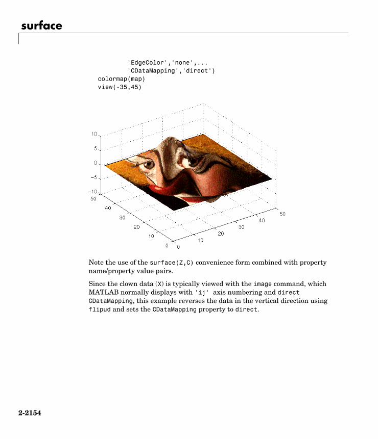
surface
2-2154
'EdgeColor','none',...'CDataMapping','direct')
colormap(map)view(-35,45)
Note the use of the surface(Z,C) convenience form combined with property name/property value pairs.
Since the clown data (X) is typically viewed with the image command, which MATLAB normally displays with 'ij' axis numbering and direct CDataMapping, this example reverses the data in the vertical direction using flipud and sets the CDataMapping property to direct.

surface
2-2155
Object Hierarchy
Setting Default PropertiesYou can set default surface properties on the axes, figure, and root levels:
set(0,'DefaultSurfaceProperty',PropertyValue...)set(gcf,'DefaultSurfaceProperty',PropertyValue...)set(gca,'DefaultSurfaceProperty',PropertyValue...)
where Property is the name of the surface property whose default value you want to set and PropertyValue is the value you are specifying. Use set and get to access the surface properties.
See Also ColorSpec, patch, pcolor, surf
Properties for surface graphics objects
“Creating Surfaces and Meshes” and “Object Creation Functions” for related functions
Surface
Axes
Surface
Group Object

Surface Properties
2-2156
2Surface PropertiesModifying Properties
You can set and query graphics object properties in two ways:
• The Property Editor is an interactive tool that enables you to see and change object property values.
• The set and get commands enable you to set and query the values of properties.
To change the default values of properties, see Setting Default Property Values.
See Core Objects for general information about this type of object.
Surface Property Descriptions
This section lists property names along with the types of values each accepts. Curly braces enclose default values.
AlphaData m-by-n matrix of double or uint8
The transparency data. A matrix of non-NaN values specifying the transparency of each face or vertex of the object. The AlphaData can be of class double or uint8.
MATLAB determines the transparency in one of three ways:
• Using the elements of AlphaData as transparency values (AlphaDataMapping set to none)
• Using the elements of AlphaData as indices into the current alphamap (AlphaDataMapping set to direct)
• Scaling the elements of AlphaData to range between the minimum and maximum values of the axes ALim property (AlphaDataMapping set to scaled, the default)
AlphaDataMapping none | direct | scaled
Transparency mapping method. This property determines how MATLAB interprets indexed alpha data. This property can be any of the following:
• none — The transparency values of AlphaData are between 0 and 1 or are clamped to this range (the default).
• scaled — Transform the AlphaData to span the portion of the alphamap indicated by the axes ALim property, linearly mapping data values to alpha values.

Surface Properties
2-2157
• direct — use the AlphaData as indices directly into the alphamap. When not scaled, the data are usually integer values ranging from 1 to length(alphamap). MATLAB maps values less than 1 to the first alpha value in the alphamap, and values greater than length(alphamap) to the last alpha value in the alphamap. Values with a decimal portion are fixed to the nearest lower integer. If AlphaData is an array of uint8 integers, then the indexing begins at 0 (i.e., MATLAB maps a value of 0 to the first alpha value in the alphamap).
AmbientStrength scalar >= 0 and <= 1
Strength of ambient light. This property sets the strength of the ambient light, which is a nondirectional light source that illuminates the entire scene. You must have at least one visible light object in the axes for the ambient light to be visible. The axes AmbientLightColor property sets the color of the ambient light, which is therefore the same on all objects in the axes.
You can also set the strength of the diffuse and specular contribution of light objects. See the surface DiffuseStrength and SpecularStrength properties.
BackFaceLighting unlit | lit | reverselit
Face lighting control. This property determines how faces are lit when their vertex normals point away from the camera.
• unlit — Face is not lit.
• lit — Face is lit in normal way.
• reverselit — Face is lit as if the vertex pointed towards the camera.
This property is useful for discriminating between the internal and external surfaces of an object. See Back Face Lighting for an example.
BeingDeleted on | off Read Only
This object is being deleted. The BeingDeleted property provides a mechanism that you can use to determine if objects are in the process of being deleted. MATLAB sets the BeingDeleted property to on when the object’s delete function callback is called (see the DeleteFcn property). It remains set to on while the delete function executes, after which the object no longer exists.
For example, an object’s delete function might call other functions that act on a number of different objects. These functions may not need to perform actions

Surface Properties
2-2158
on objects that are going to be deleted, and therefore, can check the object’s BeingDeleted property before acting.
BusyAction cancel | queue
Callback routine interruption. The BusyAction property enables you to control how MATLAB handles events that potentially interrupt executing callback routines. If there is a callback routine executing, callback routines invoked subsequently always attempt to interrupt it. If the Interruptible property of the object whose callback is executing is set to on (the default), then interruption occurs at the next point where the event queue is processed. If the Interruptible property is off, the BusyAction property (of the object owning the executing callback) determines how MATLAB handles the event. The choices are
• cancel — Discard the event that attempted to execute a second callback routine.
• queue — Queue the event that attempted to execute a second callback routine until the current callback finishes.
ButtonDownFcn string or function handle
Button press callback routine. A callback routine that executes whenever you press a mouse button while the pointer is over the surface object. Define this routine as a string that is a valid MATLAB expression or the name of an M-file. The expression executes in the MATLAB workspace.
See Function Handle Callbacks for information on how to use function handles to define the callback function.
CData matrix
Vertex colors. A matrix containing values that specify the color at every point in ZData. If you set the FaceColor property to texturemap, CData does not need to be the same size as ZData. In this case, MATLAB maps CData to conform to the surface defined by ZData.
You can specify color as indexed values or true color. Indexed color data specifies a single value for each vertex. These values are either scaled to map linearly into the current colormap (see caxis) or interpreted directly as indices into the colormap, depending on the setting of the CDataMapping property.

Surface Properties
2-2159
True color defines an RGB value for each vertex. If the coordinate data (XData, for example) are contained in m-by-n matrices, then CData must be an m-by-n-3 array. The first page contains the red components, the second the green components, and the third the blue components of the colors.
CDataMapping scaled | direct
Direct or scaled color mapping. This property determines how MATLAB interprets indexed color data used to color the surface. (If you use true color specification for CData, this property has no effect.)
• scaled — Transform the color data to span the portion of the colormap indicated by the axes CLim property, linearly mapping data values to colors. See the caxis reference page for more information on this mapping.
• direct — Use the color data as indices directly into the colormap. The color data should then be integer values ranging from 1 to length(colormap). MATLAB maps values less than 1 to the first color in the colormap, and values greater than length(colormap) to the last color in the colormap. Values with a decimal portion are fixed to the nearest lower integer.
Children matrix of handles
Always the empty matrix; surface objects have no children.
Clipping on | off
Clipping to axes rectangle. When Clipping is on, MATLAB does not display any portion of the surface that is outside the axes rectangle.
CreateFcn string or function handle
Callback routine executed during object creation. This property defines a callback routine that executes when MATLAB creates a surface object. You must define this property as a default value for surfaces or set the CreateFcn property during object creation.
For example, the following statement creates a surface (assuming x, y, z, and c are defined), and executes the function referenced by the function handle @myCreateFcn.
surface(x,y,z,c,'CreateFcn',@myCreateFcn)
MATLAB executes this routine after setting all surface properties. Setting this property on an existing surface object has no effect.

Surface Properties
2-2160
The handle of the object whose CreateFcn is being executed is accessible only through the root CallbackObject property, which you can query using gcbo.
See Function Handle Callbacks for information on how to use function handles to define the callback function.
DeleteFcn string or function handle
Delete surface callback routine. A callback routine that executes when you delete the surface object (e.g., when you issue a delete command or clear the axes or figure). MATLAB executes the routine before destroying the object’s properties so these values are available to the callback routine.
The handle of the object whose DeleteFcn is being executed is accessible only through the root CallbackObject property, which you can query using gcbo.
See Function Handle Callbacks for information on how to use function handles to define the callback function.
DiffuseStrength scalar >= 0 and <= 1
Intensity of diffuse light. This property sets the intensity of the diffuse component of the light falling on the surface. Diffuse light comes from light objects in the axes.
You can also set the intensity of the ambient and specular components of the light on the surface object. See the AmbientStrength and SpecularStrength properties.
EdgeAlpha scalar = 1 | flat | interp
Transparency of the surface edges. This property can be any of the following:
• scalar — A single non-Nan scalar value between 0 and 1 that controls the transparency of all the edges of the object. 1 (the default) means fully opaque and 0 means completely transparent.
• flat — The alpha data (AlphaData) value for the first vertex of the face determines the transparency of the edges.
• interp — Linear interpolation of the alpha data (AlphaData) values at each vertex determines the transparency of the edge.
Note that you must specify AlphaData as a matrix equal in size to ZData to use flat or interp EdgeAlpha.

Surface Properties
2-2161
EdgeColor ColorSpec | none | flat | interp
Color of the surface edge. This property determines how MATLAB colors the edges of the individual faces that make up the surface:
• ColorSpec — A three-element RGB vector or one of the MATLAB predefined names, specifying a single color for edges. The default EdgeColor is black. See ColorSpec for more information on specifying color.
• none — Edges are not drawn.
• flat — The CData value of the first vertex for a face determines the color of each edge.
• interp — Linear interpolation of the CData values at the face vertices determines the edge color.
EdgeLighting none | flat | gouraud | phong
Algorithm used for lighting calculations. This property selects the algorithm used to calculate the effect of light objects on surface edges. Choices are
• none — Lights do not affect the edges of this object.
• flat — The effect of light objects is uniform across each edge of the surface.
• gouraud — The effect of light objects is calculated at the vertices and then linearly interpolated across the edge lines.
• phong — The effect of light objects is determined by interpolating the vertex normals across each edge line and calculating the reflectance at each pixel. Phong lighting generally produces better results than Gouraud lighting, but takes longer to render.
Vertex controlling the
Direction of
Direction ofcolor of adjacent edges
increasing y data
increasing x data
Surface Properties
2-2162
EraseMode normal | none | xor | background
Erase mode. This property controls the technique MATLAB uses to draw and erase surface objects. Alternative erase modes are useful for creating animated sequences, where control of the way individual objects are redrawn is necessary to improve performance and obtain the desired effect.
• normal — Redraw the affected region of the display, performing the three-dimensional analysis necessary to ensure that all objects are rendered correctly. This mode produces the most accurate picture, but is the slowest. The other modes are faster, but do not perform a complete redraw and are therefore less accurate.
• none — Do not erase the surface when it is moved or destroyed. While the object is still visible on the screen after erasing with EraseMode none, you cannot print it because MATLAB stores no information about its former location.
• xor — Draw and erase the surface by performing an exclusive OR (XOR) with each pixel index of the screen behind it. Erasing the surface does not damage the color of the objects behind it. However, surface color depends on the color of the screen behind it and is correctly colored only when over the axes background Color, or the figure background Color if the axes Color is set to none.
• background — Erase the surface by drawing it in the axes background Color, or the figure background Color if the axes Color is set to none. This damages objects that are behind the erased object, but surface objects are always properly colored.
Printing with Nonnormal Erase Modes. MATLAB always prints figures as if the EraseMode of all objects is normal. This means graphics objects created with EraseMode set to none, xor, or background can look different on screen than on paper. On screen, MATLAB may mathematically combine layers of colors (e.g., performing an XOR of a pixel color with that of the pixel behind it) and ignore three-dimensional sorting to obtain greater rendering speed. However, these techniques are not applied to the printed output.
You can use the MATLAB getframe command or other screen capture application to create an image of a figure containing nonnormal mode objects.

Surface Properties
2-2163
FaceAlpha scalar = 1 | flat | interp | texturemap
Transparency of the surface faces. This property can be any of the following:
• scalar — A single non-NaN scalar value between 0 and 1 that controls the transparency of all the faces of the object. 1 (the default) means fully opaque and 0 means completely transparent (invisible).
• flat — The values of the alpha data (AlphaData) determine the transparency for each face. The alpha data at the first vertex determine the transparency of the entire face.
• interp — Bilinear interpolation of the alpha data (AlphaData) at each vertex determines the transparency of each face.
• texturemap — Use transparency for the texture map.
Note that you must specify AlphaData as a matrix equal in size to ZData to use flat or interp FaceAlpha.
FaceColor ColorSpec | none | flat | interp
Color of the surface face. This property can be any of the following:
• ColorSpec — A three-element RGB vector or one of the MATLAB predefined names, specifying a single color for faces. See ColorSpec for more information on specifying color.
• none — Do not draw faces. Note that edges are drawn independently of faces.
• flat — The values of CData determine the color for each face of the surface. The color data at the first vertex determine the color of the entire face.
• interp — Bilinear interpolation of the values at each vertex (the CData) determines the coloring of each face.
• texturemap — Texture map the CData to the surface. MATLAB transforms the color data so that it conforms to the surface. (See the texture mapping example.)
FaceLighting none | flat | gouraud | phong
Algorithm used for lighting calculations. This property selects the algorithm used to calculate the effect of light objects on the surface. Choices are
• none — Lights do not affect the faces of this object.
• flat — The effect of light objects is uniform across the faces of the surface. Select this choice to view faceted objects.

Surface Properties
2-2164
• gouraud — The effect of light objects is calculated at the vertices and then linearly interpolated across the faces. Select this choice to view curved surfaces.
• phong — The effect of light objects is determined by interpolating the vertex normals across each face and calculating the reflectance at each pixel. Select this choice to view curved surfaces. Phong lighting generally produces better results than Gouraud lighting, but takes longer to render.
HandleVisibility on | callback | off
Control access to object’s handle by command-line users and GUIs. This property determines when an object’s handle is visible in its parent’s list of children. This property is useful for preventing command-line users from accidentally drawing into or deleting a figure that contains only user interface devices (such as a dialog box).
Handles are always visible when HandleVisibility is on.
Setting HandleVisibility to callback causes handles to be visible from within callback routines or functions invoked by callback routines, but not from within functions invoked from the command line. This provides a means to protect GUIs from command-line users, while allowing callback routines to have complete access to object handles.
Setting HandleVisibility to off makes handles invisible at all times. This might be necessary when a callback routine invokes a function that could potentially damage the GUI (such as evaluating a user-typed string), and so temporarily hides its own handles during the execution of that function.
When a handle is not visible in its parent’s list of children, it cannot be returned by functions that obtain handles by searching the object hierarchy or querying handle properties. This includes get, findobj, gca, gcf, gco, newplot, cla, clf, and close.
When a handle’s visibility is restricted using callback or off, the object’s handle does not appear in its parent’s Children property, figures do not appear in the root’s CurrentFigure property, objects do not appear in the root’s CallbackObject property or in the figure’s CurrentObject property, and axes do not appear in their parent’s CurrentAxes property.

Surface Properties
2-2165
You can set the root ShowHiddenHandles property to on to make all handles visible, regardless of their HandleVisibility settings (this does not affect the values of the HandleVisibility properties).
Handles that are hidden are still valid. If you know an object’s handle, you can set and get its properties, and pass it to any function that operates on handles.
HitTest on | off
Selectable by mouse click. HitTest determines if the surface can become the current object (as returned by the gco command and the figure CurrentObject property) as a result of a mouse click on the surface. If HitTest is off, clicking on the surface selects the object below it (which may be the axes containing it).
Interruptible on | off
Callback routine interruption mode. The Interruptible property controls whether a surface callback routine can be interrupted by subsequently invoked callback routines. Only callback routines defined for the ButtonDownFcn are affected by the Interruptible property. MATLAB checks for events that can interrupt a callback routine only when it encounters a drawnow, figure, getframe, or pause command in the routine. See the BusyAction property for related information.
LineStyle - | -- | : | -. | none
Edge line type. This property determines the line style used to draw surface edges. The available line styles are shown in this table.
Symbol Line Style
Solid line (default)
Dashed line
: Dotted line
. Dash-dot line
none No line

Surface Properties
2-2166
LineWidth scalar
Edge line width. The width of the lines in points used to draw surface edges. The default width is 0.5 points (1 point = 1/72 inch).
Marker marker symbol (see table)
Marker symbol. The Marker property specifies symbols that are displayed at vertices. You can set values for the Marker property independently from the LineStyle property.
You can specify these markers.
Marker Specifier Description
+ Plus sign
o Circle
* Asterisk
. Point
x Cross
s Square
d Diamond
^ Upward-pointing triangle
v Downward-pointing triangle
> Right-pointing triangle
< Left-pointing triangle
p Five-pointed star (pentagram)
h Six-pointed star (hexagram)
none No marker (default)

Surface Properties
2-2167
MarkerEdgeColor none | auto | flat | ColorSpec
Marker edge color. The color of the marker or the edge color for filled markers (circle, square, diamond, pentagram, hexagram, and the four triangles).
• none specifies no color, which makes nonfilled markers invisible.
• auto uses the same color as the EdgeColor property.
• flat uses the CData value of the vertex to determine the color of the maker edge.
• ColorSpec defines a single color to use for the edge (see ColorSpec for more information).
MarkerFaceColor none | auto | flat | ColorSpec
Marker face color. The fill color for markers that are closed shapes (circle, square, diamond, pentagram, hexagram, and the four triangles).
• none makes the interior of the marker transparent, allowing the background to show through.
• auto uses the axes Color for the marker face color.
• flat uses the CData value of the vertex to determine the color of the face.
• ColorSpec defines a single color to use for all markers on the surface (see ColorSpec for more information).
MarkerSize size in points
Marker size. A scalar specifying the marker size, in points. The default value for MarkerSize is 6 points (1 point = 1/72 inch). Note that MATLAB draws the point marker at 1/3 the specified marker size.
MeshStyle both | row | column
Row and column lines. This property specifies whether to draw all edge lines or just row or column edge lines.
• both draws edges for both rows and columns.
• row draws row edges only.
• column draws column edges only.
NormalMode auto | manual
MATLAB generated or user-specified normal vectors. When this property is auto, MATLAB calculates vertex normals based on the coordinate data. If you

Surface Properties
2-2168
specify your own vertex normals, MATLAB sets this property to manual and does not generate its own data. See also the VertexNormals property.
Parent handle of axes, hggroup, or hgtransform
Parent of surface object. This property contains the handle of the surface object’s parent. The parent of a surface object is the axes, hggroup, or hgtransform object that contains it.
See Objects That Can Contain Other Objects for more information on parenting graphics objects.
Selected on | off
Is object selected? When this property is on, MATLAB displays a dashed bounding box around the surface if the SelectionHighlight property is also on. You can, for example, define the ButtonDownFcn to set this property, allowing users to select the object with the mouse.
SelectionHighlight on | off
Objects are highlighted when selected. When the Selected property is on, MATLAB indicates the selected state by drawing a dashed bounding box around the surface. When SelectionHighlight is off, MATLAB does not draw the handles.
SpecularColorReflectancescalar in the range 0 to 1
Color of specularly reflected light. When this property is 0, the color of the specularly reflected light depends on both the color of the object from which it reflects and the color of the light source. When set to 1, the color of the specularly reflected light depends only on the color or the light source (i.e., the light object Color property). The proportions vary linearly for values in between.
SpecularExponent scalar >= 1
Harshness of specular reflection. This property controls the size of the specular spot. Most materials have exponents in the range of 5 to 20.
SpecularStrength scalar >= 0 and <= 1
Intensity of specular light. This property sets the intensity of the specular component of the light falling on the surface. Specular light comes from light objects in the axes.

Surface Properties
2-2169
You can also set the intensity of the ambient and diffuse components of the light on the surface object. See the AmbientStrength and DiffuseStrength properties. Also see the material function.
Tag string
User-specified object label. The Tag property provides a means to identify graphics objects with a user-specified label. This is particularly useful when you are constructing interactive graphics programs that would otherwise need to define object handles as global variables or pass them as arguments between callback routines. You can define Tag as any string.
Type string (read only)
Class of the graphics object. The class of the graphics object. For surface objects, Type is always the string 'surface'.
UIContextMenu handle of a uicontextmenu object
Associate a context menu with the surface. Assign this property the handle of a uicontextmenu object created in the same figure as the surface. Use the uicontextmenu function to create the context menu. MATLAB displays the context menu whenever you right-click over the surface.
UserData matrix
User-specified data. Any matrix you want to associate with the surface object. MATLAB does not use this data, but you can access it using the set and get commands.
VertexNormals vector or matrix
Surface normal vectors. This property contains the vertex normals for the surface. MATLAB generates this data to perform lighting calculations. You can supply your own vertex normal data, even if it does not match the coordinate data. This can be useful to produce interesting lighting effects.
Visible on | off
Surface object visibility. By default, all surfaces are visible. When set to off, the surface is not visible, but still exists, and you can query and set its properties.

Surface Properties
2-2170
XData vector or matrix
X-coordinates. The x-position of the surface points. If you specify a row vector, surface replicates the row internally until it has the same number of columns as ZData.
YData vector or matrix
Y-coordinates. The y-position of the surface points. If you specify a row vector, surface replicates the row internally until it has the same number of rows as ZData.
ZData matrix
Z-coordinates. The z-position of the surface points. See the Description section for more information.

Surfaceplot Properties
2-2171
2Surfaceplot PropertiesModifying Properties
You can set and query graphics object properties in two ways:
• The Property Editor is an interactive tool that enables you to see and change object property values.
• The set and get commands enable you to set and query the values of properties.
Note that you cannot define default properties for surfaceplot objects.
See Plot Objects for information on surfaceplot objects.
Surfaceplot Property Descriptions
This section lists property names along with the types of values each accepts. Curly braces enclose default values.
AlphaData m-by-n matrix of double or uint8
The transparency data. A matrix of non-NaN values specifying the transparency of each face or vertex of the object. The AlphaData can be of class double or uint8.
MATLAB determines the transparency in one of three ways:
• Using the elements of AlphaData as transparency values (AlphaDataMapping set to none)
• Using the elements of AlphaData as indices into the current alphamap (AlphaDataMapping set to direct)
• Scaling the elements of AlphaData to range between the minimum and maximum values of the axes ALim property (AlphaDataMapping set to scaled, the default)
AlphaDataMapping none | direct | scaled
Transparency mapping method. This property determines how MATLAB interprets indexed alpha data. This property can be any of the following:
• none — The transparency values of AlphaData are between 0 and 1 or are clamped to this range (the default).
• scaled — Transform the AlphaData to span the portion of the alphamap indicated by the axes ALim property, linearly mapping data values to alpha values.
• direct — use the AlphaData as indices directly into the alphamap. When not scaled, the data are usually integer values ranging from 1 to

Surfaceplot Properties
2-2172
length(alphamap). MATLAB maps values less than 1 to the first alpha value in the alphamap, and values greater than length(alphamap) to the last alpha value in the alphamap. Values with a decimal portion are fixed to the nearest lower integer. If AlphaData is an array of uint8 integers, then the indexing begins at 0 (i.e., MATLAB maps a value of 0 to the first alpha value in the alphamap).
AmbientStrength scalar >= 0 and <= 1
Strength of ambient light. This property sets the strength of the ambient light, which is a nondirectional light source that illuminates the entire scene. You must have at least one visible light object in the axes for the ambient light to be visible. The axes AmbientLightColor property sets the color of the ambient light, which is therefore the same on all objects in the axes.
You can also set the strength of the diffuse and specular contribution of light objects. See the surfaceplot DiffuseStrength and SpecularStrength properties.
BackFaceLighting unlit | lit | reverselit
Face lighting control. This property determines how faces are lit when their vertex normals point away from the camera.
• unlit — Face is not lit.
• lit — Face is lit in normal way.
• reverselit — Face is lit as if the vertex pointed towards the camera.
This property is useful for discriminating between the internal and external surfaces of an object. See Back Face Lighting for an example.
BeingDeleted on | off Read Only
This object is being deleted. The BeingDeleted property provides a mechanism that you can use to determine if objects are in the process of being deleted. MATLAB sets the BeingDeleted property to on when the object’s delete function callback is called (see the DeleteFcn property). It remains set to on while the delete function executes, after which the object no longer exists.
For example, an object’s delete function might call other functions that act on a number of different objects. These functions may not need to perform actions on objects that are going to be deleted, and therefore, can check the object’s BeingDeleted property before acting.

Surfaceplot Properties
2-2173
BusyAction cancel | queue
Callback routine interruption. The BusyAction property enables you to control how MATLAB handles events that potentially interrupt executing callback routines. If there is a callback routine executing, callback routines invoked subsequently always attempt to interrupt it. If the Interruptible property of the object whose callback is executing is set to on (the default), then interruption occurs at the next point where the event queue is processed. If the Interruptible property is off, the BusyAction property (of the object owning the executing callback) determines how MATLAB handles the event. The choices are
• cancel — Discard the event that attempted to execute a second callback routine.
• queue — Queue the event that attempted to execute a second callback routine until the current callback finishes.
ButtonDownFcn string or function handle
Button press callback routine. A callback routine that executes whenever you press a mouse button while the pointer is over the surfaceplot object. Define this routine as a string that is a valid MATLAB expression or the name of an M-file. The expression executes in the MATLAB workspace.
See Function Handle Callbacks for information on how to use function handles to define the callback function.
CData matrix
Vertex colors. A matrix containing values that specify the color at every point in ZData. If you set the FaceColor property to texturemap, CData does not need to be the same size as ZData. In this case, MATLAB maps CData to conform to the surfaceplot defined by ZData.
You can specify color as indexed values or true color. Indexed color data specifies a single value for each vertex. These values are either scaled to map linearly into the current colormap (see caxis) or interpreted directly as indices into the colormap, depending on the setting of the CDataMapping property.
True color defines an RGB value for each vertex. If the coordinate data (XData, for example) are contained in m-by-n matrices, then CData must be an m-by-n-3 array. The first page contains the red components, the second the green components, and the third the blue components of the colors.

Surfaceplot Properties
2-2174
CDataMapping scaled | direct
Direct or scaled color mapping. This property determines how MATLAB interprets indexed color data used to color the surfaceplot. (If you use true color specification for CData, this property has no effect.)
• scaled — Transform the color data to span the portion of the colormap indicated by the axes CLim property, linearly mapping data values to colors. See the caxis reference page for more information on this mapping.
• direct — Use the color data as indices directly into the colormap. The color data should then be integer values ranging from 1 to length(colormap). MATLAB maps values less than 1 to the first color in the colormap, and values greater than length(colormap) to the last color in the colormap. Values with a decimal portion are fixed to the nearest lower integer.
CDataMode auto | manual
Use automatic or user-specified color data values. If you specify CData, MATLAB sets this property to manual and uses the CData values to color the surfaceplot.
If you set CDataMode to auto after having specified CData, MATLAB resets the color data of the surfaceplot to that defined by ZData, overwriting any previous values for CData.
CDataSource string (MATLAB variable)
Link CData to MATLAB variable. Set this property to a MATLAB variable that is evaluated in the base workspace to generate the CData.
MATLAB reevaluates this property only when you set it. Therefore, a change to workspace variables appearing in an expression does not change CData.
You can use the refreshdata function to force an update of the object’s data. refreshdata also enables you to specify that the data source variable be evaluated in the workspace of a function from which you call refreshdata.
See the refreshdata reference page for more information.

Surfaceplot Properties
2-2175
Note If you change one data source property to return data of a different dimension, you might cause the function to generate a warning and not render the graph until you have changed all data source properties to appropriate values.
Children matrix of handles
Always the empty matrix; surfaceplot objects have no children.
Clipping on | off
Clipping to axes rectangle. When Clipping is on, MATLAB does not display any portion of the surfaceplot that is outside the axes rectangle.
CreateFcn string or function handle
Callback routine executed during object creation. This property defines a callback that executes when MATLAB creates a surfaceplot object. You must specify the callback during the creation of the object. For example,
surf(peaks,'CreateFcn',@CallbackFcn)
where @CallbackFcn is a function handle that references the callback function.
MATLAB executes this routine after setting all other surfaceplot properties. Setting this property on an existing surfaceplot object has no effect.
The handle of the object whose CreateFcn is being executed is accessible only through the root CallbackObject property, which you can query using gcbo.
See Function Handle Callbacks for information on how to use function handles to define the callback function.
DeleteFcn string or function handle
Delete surfaceplot callback routine. A callback routine that executes when you delete the surfaceplot object (e.g., when you issue a delete command or clear the axes or figure). MATLAB executes the routine before destroying the object’s properties so these values are available to the callback routine.
The handle of the object whose DeleteFcn is being executed is accessible only through the root CallbackObject property, which you can query using gcbo.

Surfaceplot Properties
2-2176
See Function Handle Callbacks for information on how to use function handles to define the callback function.
DiffuseStrength scalar >= 0 and <= 1
Intensity of diffuse light. This property sets the intensity of the diffuse component of the light falling on the surface. Diffuse light comes from light objects in the axes.
You can also set the intensity of the ambient and specular components of the light on the surfaceplot object. See the AmbientStrength and SpecularStrength properties.
EdgeAlpha scalar = 1 | flat | interp
Transparency of the surfaceplot edges. This property can be any of the following:
• scalar — A single non-Nan scalar value between 0 and 1 that controls the transparency of all the edges of the object. 1 (the default) means fully opaque and 0 means completely transparent.
• flat — The alpha data (AlphaData) value for the first vertex of the face determines the transparency of the edges.
• interp — Linear interpolation of the alpha data (AlphaData) values at each vertex determines the transparency of the edge.
Note that you must specify AlphaData as a matrix equal in size to ZData to use flat or interp EdgeAlpha.
EdgeColor ColorSpec | none | flat | interp
Color of the surfaceplot edge. This property determines how MATLAB colors the edges of the individual faces that make up the surface:
• ColorSpec — A three-element RGB vector or one of the MATLAB predefined names, specifying a single color for edges. The default EdgeColor is black. See ColorSpec for more information on specifying color.
• none — Edges are not drawn.

Surfaceplot Properties
2-2177
• flat — The CData value of the first vertex for a face determines the color of each edge.
• interp — Linear interpolation of the CData values at the face vertices determines the edge color.
EdgeLighting none | flat | gouraud | phong
Algorithm used for lighting calculations. This property selects the algorithm used to calculate the effect of light objects on surfaceplot edges. Choices are
• none — Lights do not affect the edges of this object.
• flat — The effect of light objects is uniform across each edge of the surface.
• gouraud — The effect of light objects is calculated at the vertices and then linearly interpolated across the edge lines.
• phong — The effect of light objects is determined by interpolating the vertex normals across each edge line and calculating the reflectance at each pixel. Phong lighting generally produces better results than Gouraud lighting, but takes longer to render.
EraseMode normal | none | xor | background
Erase mode. This property controls the technique MATLAB uses to draw and erase surfaceplot objects. Alternative erase modes are useful for creating animated sequences, where control of the way individual objects are redrawn is necessary to improve performance and obtain the desired effect.
• normal — Redraw the affected region of the display, performing the three-dimensional analysis necessary to ensure that all objects are rendered correctly. This mode produces the most accurate picture, but is the slowest. The other modes are faster, but do not perform a complete redraw and are therefore less accurate.
Vertex controlling the
Direction of
Direction ofcolor of adjacent edges
increasing y data
increasing x data

Surfaceplot Properties
2-2178
• none — Do not erase the surfaceplot when it is moved or destroyed. While the object is still visible on the screen after erasing with EraseMode none, you cannot print it because MATLAB stores no information about its former location.
• xor — Draw and erase the surfaceplot by performing an exclusive OR (XOR) with each pixel index of the screen behind it. Erasing the surfaceplot does not damage the color of the objects behind it. However, surfaceplot color depends on the color of the screen behind it and is correctly colored only when over the axes background Color, or the figure background Color if the axes Color is set to none.
• background — Erase the surfaceplot by drawing it in the axes background Color, or the figure background Color if the axes Color is set to none. This damages objects that are behind the erased object, but surfaceplot objects are always properly colored.
Printing with Nonnormal Erase Modes. MATLAB always prints figures as if the EraseMode of all objects is normal. This means graphics objects created with EraseMode set to none, xor, or background can look different on screen than on paper. On screen, MATLAB may mathematically combine layers of colors (e.g., performing an XOR of a pixel color with that of the pixel behind it) and ignore three-dimensional sorting to obtain greater rendering speed. However, these techniques are not applied to the printed output.
You can use the MATLAB getframe command or other screen capture application to create an image of a figure containing nonnormal mode objects.
FaceAlpha scalar = 1 | flat | interp | texturemap
Transparency of the surfaceplot faces. This property can be any of the following:
• scalar — A single non-NaN scalar value between 0 and 1 that controls the transparency of all the faces of the object. 1 (the default) means fully opaque and 0 means completely transparent (invisible).
• flat — The values of the alpha data (AlphaData) determine the transparency for each face. The alpha data at the first vertex determine the transparency of the entire face.
• interp — Bilinear interpolation of the alpha data (AlphaData) at each vertex determines the transparency of each face.
• texturemap — Use transparency for the texture map.

Surfaceplot Properties
2-2179
Note that you must specify AlphaData as a matrix equal in size to ZData to use flat or interp FaceAlpha.
FaceColor ColorSpec | none | flat | interp
Color of the surfaceplot face. This property can be any of the following:
• ColorSpec — A three-element RGB vector or one of the MATLAB predefined names, specifying a single color for faces. See ColorSpec for more information on specifying color.
• none — Do not draw faces. Note that edges are drawn independently of faces.
• flat — The values of CData determine the color for each face of the surface. The color data at the first vertex determine the color of the entire face.
• interp — Bilinear interpolation of the values at each vertex (the CData) determines the coloring of each face.
• texturemap — Texture map the CData to the surface. MATLAB transforms the color data so that it conforms to the surface. (See the texture mapping example.)
FaceLighting none | flat | gouraud | phong
Algorithm used for lighting calculations. This property selects the algorithm used to calculate the effect of light objects on the surface. Choices are
• none — Lights do not affect the faces of this object.
• flat — The effect of light objects is uniform across the faces of the surface. Select this choice to view faceted objects.
• gouraud — The effect of light objects is calculated at the vertices and then linearly interpolated across the faces. Select this choice to view curved surfaces.
• phong — The effect of light objects is determined by interpolating the vertex normals across each face and calculating the reflectance at each pixel. Select this choice to view curved surfaces. Phong lighting generally produces better results than Gouraud lighting, but takes longer to render.
HandleVisibility on | callback | off
Control access to object’s handle by command-line users and GUIs. This property determines when an object’s handle is visible in its parent’s list of children. This property is useful for preventing command-line users from

Surfaceplot Properties
2-2180
accidentally drawing into or deleting a figure that contains only user interface devices (such as a dialog box).
Handles are always visible when HandleVisibility is on.
Setting HandleVisibility to callback causes handles to be visible from within callback routines or functions invoked by callback routines, but not from within functions invoked from the command line. This provides a means to protect GUIs from command-line users, while allowing callback routines to have complete access to object handles.
Setting HandleVisibility to off makes handles invisible at all times. This might be necessary when a callback routine invokes a function that could potentially damage the GUI (such as evaluating a user-typed string), and so temporarily hides its own handles during the execution of that function.
When a handle is not visible in its parent’s list of children, it cannot be returned by functions that obtain handles by searching the object hierarchy or querying handle properties. This includes get, findobj, gca, gcf, gco, newplot, cla, clf, and close.
When a handle’s visibility is restricted using callback or off, the object’s handle does not appear in its parent’s Children property, figures do not appear in the root’s CurrentFigure property, objects do not appear in the root’s CallbackObject property or in the figure’s CurrentObject property, and axes do not appear in their parent’s CurrentAxes property.
You can set the root ShowHiddenHandles property to on to make all handles visible, regardless of their HandleVisibility settings (this does not affect the values of the HandleVisibility properties).
Handles that are hidden are still valid. If you know an object’s handle, you can set and get its properties, and pass it to any function that operates on handles.
HitTest on | off
Selectable by mouse click. HitTest determines if the surfaceplot can become the current object (as returned by the gco command and the figure CurrentObject property) as a result of a mouse click on the surface. If HitTest is off, clicking on the surfaceplot selects the object below it (which may be the axes containing it).

Surfaceplot Properties
2-2181
Interruptible on | off
Callback routine interruption mode. The Interruptible property controls whether a surfaceplot callback routine can be interrupted by subsequently invoked callback routines. Only callback routines defined for the ButtonDownFcn are affected by the Interruptible property. MATLAB checks for events that can interrupt a callback routine only when it encounters a drawnow, figure, getframe, or pause command in the routine. See the BusyAction property for related information.
LineStyle - | -- | : | -. | none
Edge line type. This property determines the line style used to draw surfaceplot edges. The available line styles are shown in this table.
LineWidth scalar
Edge line width. The width of the lines in points used to draw surfaceplot edges. The default width is 0.5 points (1 point = 1/72 inch).
Marker marker symbol (see table)
Marker symbol. The Marker property specifies symbols that are displayed at vertices. You can set values for the Marker property independently from the LineStyle property.
Symbol Line Style
Solid line (default)
Dashed line
: Dotted line
. Dash-dot line
none No line

Surfaceplot Properties
2-2182
You can specify these markers.
MarkerEdgeColor none | auto | flat | ColorSpec
Marker edge color. The color of the marker or the edge color for filled markers (circle, square, diamond, pentagram, hexagram, and the four triangles).
• none specifies no color, which makes nonfilled markers invisible.
• auto uses the same color as the EdgeColor property.
• flat uses the CData value of the vertex to determine the color of the maker edge.
• ColorSpec defines a single color to use for the edge (see ColorSpec for more information).
Marker Specifier Description
+ Plus sign
o Circle
* Asterisk
. Point
x Cross
s Square
d Diamond
^ Upward-pointing triangle
v Downward-pointing triangle
> Right-pointing triangle
< Left-pointing triangle
p Five-pointed star (pentagram)
h Six-pointed star (hexagram)
none No marker (default)

Surfaceplot Properties
2-2183
MarkerFaceColor none | auto | flat | ColorSpec
Marker face color. The fill color for markers that are closed shapes (circle, square, diamond, pentagram, hexagram, and the four triangles).
• none makes the interior of the marker transparent, allowing the background to show through.
• auto uses the axes Color for the marker face color.
• flat uses the CData value of the vertex to determine the color of the face.
• ColorSpec defines a single color to use for all markers on the surfaceplot (see ColorSpec for more information).
MarkerSize size in points
Marker size. A scalar specifying the marker size, in points. The default value for MarkerSize is 6 points (1 point = 1/72 inch). Note that MATLAB draws the point marker at 1/3 the specified marker size.
MeshStyle both | row | column
Row and column lines. This property specifies whether to draw all edge lines or just row or column edge lines.
• both draws edges for both rows and columns.
• row draws row edges only.
• column draws column edges only.
NormalMode auto | manual
MATLAB generated or user-specified normal vectors. When this property is auto, MATLAB calculates vertex normals based on the coordinate data. If you specify your own vertex normals, MATLAB sets this property to manual and does not generate its own data. See also the VertexNormals property.
Parent handle of axes, hggroup, or hgtransform
Parent of surfaceplot object. This property contains the handle of the surfaceplot object’s parent. The parent of a surfaceplot object is the axes, hggroup, or hgtransform object that contains it.
See Objects That Can Contain Other Objects for more information on parenting graphics objects.

Surfaceplot Properties
2-2184
Selected on | off
Is object selected? When this property is on, MATLAB displays a dashed bounding box around the surfaceplot if the SelectionHighlight property is also on. You can, for example, define the ButtonDownFcn to set this property, allowing users to select the object with the mouse.
SelectionHighlight on | off
Objects are highlighted when selected. When the Selected property is on, MATLAB indicates the selected state by drawing a dashed bounding box around the surface. When SelectionHighlight is off, MATLAB does not draw the handles.
SpecularColorReflectancescalar in the range 0 to 1
Color of specularly reflected light. When this property is 0, the color of the specularly reflected light depends on both the color of the object from which it reflects and the color of the light source. When set to 1, the color of the specularly reflected light depends only on the color or the light source (i.e., the light object Color property). The proportions vary linearly for values in between.
SpecularExponent scalar >= 1
Harshness of specular reflection. This property controls the size of the specular spot. Most materials have exponents in the range of 5 to 20.
SpecularStrength scalar >= 0 and <= 1
Intensity of specular light. This property sets the intensity of the specular component of the light falling on the surface. Specular light comes from light objects in the axes.
You can also set the intensity of the ambient and diffuse components of the light on the surfaceplot object. See the AmbientStrength and DiffuseStrength properties. Also see the material function.
Tag string
User-specified object label. The Tag property provides a means to identify graphics objects with a user-specified label. This is particularly useful when you are constructing interactive graphics programs that would otherwise need to define object handles as global variables or pass them as arguments between callback routines. You can define Tag as any string.

Surfaceplot Properties
2-2185
Type string (read only)
Class of the graphics object. The class of the graphics object. For surfaceplot objects, Type is always the string 'surface'.
UIContextMenu handle of a uicontextmenu object
Associate a context menu with the surface. Assign this property the handle of a uicontextmenu object created in the same figure as the surface. Use the uicontextmenu function to create the context menu. MATLAB displays the context menu whenever you right-click over the surface.
UserData matrix
User-specified data. Any matrix you want to associate with the surfaceplot object. MATLAB does not use this data, but you can access it using the set and get commands.
VertexNormals vector or matrix
Surfaceplot normal vectors. This property contains the vertex normals for the surfaceplot. MATLAB generates this data to perform lighting calculations. You can supply your own vertex normal data, even if it does not match the coordinate data. This can be useful to produce interesting lighting effects.
Visible on | off
Surfaceplot object visibility. By default, all surfaceplots are visible. When set to off, the surfaceplot is not visible, but still exists, and you can query and set its properties.
XData vector or matrix
X-coordinates. The x-position of the surfaceplot data points. If you specify a row vector, MATLAB replicates the row internally until it has the same number of columns as ZData.
XDataMode auto | manual
Use automatic or user-specified x-axis values. If you specify XData, MATLAB sets this property to manual.
If you set XDataMode to auto after having specified XData, MATLAB resets the x-axis ticks and x-tick labels to the column indices of the ZData, overwriting any previous values for XData.

Surfaceplot Properties
2-2186
XDataSource string (MATLAB variable)
Link XData to MATLAB variable. Set this property to a MATLAB variable that is evaluated in the base workspace to generate the XData.
MATLAB reevaluates this property only when you set it. Therefore, a change to workspace variables appearing in an expression does not change XData.
You can use the refreshdata function to force an update of the object’s data. refreshdata also enables you to specify that the data source variable be evaluated in the workspace of a function from which you call refreshdata.
See the refreshdata reference page for more information.
Note If you change one data source property to return data of a different dimension, you might cause the function to generate a warning and not render the graph until you have changed all data source properties to appropriate values.
YData vector or matrix
Y-coordinates. The y-position of the surfaceplot data points. If you specify a row vector, MATLAB replicates the row internally until it has the same number of rows as ZData.
YDataMode auto | manual
Use automatic or user-specified x-axis values. If you specify XData, MATLAB sets this property to manual.
If you set YDataMode to auto after having specified YData, MATLAB resets the y-axis ticks and y-tick labels to the row indices of the ZData, overwriting any previous values for YData.
YDataSource string (MATLAB variable)
Link YData to MATLAB variable. Set this property to a MATLAB variable that is evaluated in the base workspace to generate the YData.
MATLAB reevaluates this property only when you set it. Therefore, a change to workspace variables appearing in an expression does not change YData.

Surfaceplot Properties
2-2187
You can use the refreshdata function to force an update of the object’s data. refreshdata also enables you to specify that the data source variable be evaluated in the workspace of a function from which you call refreshdata.
See the refreshdata reference page for more information.
Note If you change one data source property to a variable that contains data of a different dimension, you might cause the function to generate a warning and not render the graph until you have changed all data source properties to appropriate values.
ZData matrix
Z-coordinates. The z-position of the surfaceplot data points. See the Description section for more information.
ZDataSource string (MATLAB variable)
Link YData to MATLAB variable. Set this property to a MATLAB variable that is evaluated in the base workspace to generate the ZData.
MATLAB reevaluates this property only when you set it. Therefore, a change to workspace variables appearing in an expression does not change ZData.
You can use the refreshdata function to force an update of the object’s data. refreshdata also enables you to specify that the data source variable be evaluated in the workspace of a function from which you call refreshdata.
See the refreshdata reference page for more information.
Note If you change one data source property to a variable that contains data of a different dimension, you might cause the function to generate a warning and not render the graph until you have changed all data source properties to appropriate values.

surfl
2-2188
2surfl Purpose Surface plot with colormap-based lighting
Syntax surfl(Z)surfl(X,Y,Z)surfl(...,'light')surfl(...,s)surfl(X,Y,Z,s,k)h = surfl(...)
Description The surfl function displays a shaded surface based on a combination of ambient, diffuse, and specular lighting models.
surfl(Z) and surfl(X,Y,Z) create three-dimensional shaded surfaces using the default direction for the light source and the default lighting coefficients for the shading model. X, Y, and Z are vectors or matrices that define the x, y, and z components of a surface.
surfl(...,'light') produces a colored, lighted surface using a MATLAB light object. This produces results different from the default lighting method, surfl(...,'cdata'), which changes the color data for the surface to be the reflectance of the surface.
surfl(...,s) specifies the direction of the light source. s is a two- or three-element vector that specifies the direction from a surface to a light source. s = [sx sy sz] or s = [azimuth elevation]. The default s is 45° counterclockwise from the current view direction.
surfl(X,Y,Z,s,k) specifies the reflectance constant. k is a four-element vector defining the relative contributions of ambient light, diffuse reflection, specular reflection, and the specular shine coefficient. k = [ka kd ks shine] and defaults to [.55,.6,.4,10].
h = surfl(...) returns a handle to a surface graphics object.
Remarks For smoother color transitions, use colormaps that have linear intensity variations (e.g., gray, copper, bone, pink).
The ordering of points in the X, Y, and Z matrices defines the inside and outside of parametric surfaces. If you want the opposite side of the surface to reflect the

surfl
2-2189
light source, use surfl(X',Y',Z'). Because of the way surface normal vectors are computed, surfl requires matrices that are at least 3-by-3.
Examples View peaks using colormap-based lighting.
[x,y] = meshgrid( 3:1/8:3);z = peaks(x,y);surfl(x,y,z);shading interpcolormap(gray);axis([ 3 3 3 3 8 8])
To plot a lighted surface from a view direction other than the default,
view([10 10])grid onhold onsurfl(peaks)shading interpcolormap copperhold off

surfl
2-2190
See Also colormap, shading, light
“Creating Surfaces and Meshes” for functions related to surfaces
“Lighting” for functions related to lighting

surfnorm
2-2191
2surfnormPurpose Compute and display 3-D surface normals
Syntax surfnorm(Z)surfnorm(X,Y,Z)[Nx,Ny,Nz] = surfnorm(...)
Description The surfnorm function computes surface normals for the surface defined by X, Y, and Z. The surface normals are unnormalized and valid at each vertex. Normals are not shown for surface elements that face away from the viewer.
surfnorm(Z) and surfnorm(X,Y,Z) plot a surface and its surface normals. Z is a matrix that defines the z component of the surface. X and Y are vectors or matrices that define the x and y components of the surface.
[Nx,Ny,Nz] = surfnorm(...) returns the components of the three-dimensional surface normals for the surface.
Remarks The direction of the normals is reversed by calling surfnorm with transposed arguments:
surfnorm(X',Y',Z')
surfl uses surfnorm to compute surface normals when calculating the reflectance of a surface.
Algorithm The surface normals are based on a bicubic fit of the data in X, Y, and Z. For each vertex, diagonal vectors are computed and crossed to form the normal.
Examples Plot the normal vectors for a truncated cone.
[x,y,z] = cylinder(1:10);surfnorm(x,y,z)axis([−12 12 −12 12 −0.1 1])

surfnorm
2-2192
See Also surf, quiver3
“Colormaps” for related functions
−10−5
05
10
−10−5
05
10
0
0.2
0.4
0.6
0.8
1

svd
2-2193
2svdPurpose Singular value decomposition
Syntax s = svd(X)[U,S,V] = svd(X)[U,S,V] = svd(X,0)
Description The svd command computes the matrix singular value decomposition.
s = svd(X) returns a vector of singular values.
[U,S,V] = svd(X) produces a diagonal matrix S of the same dimension as X, with nonnegative diagonal elements in decreasing order, and unitary matrices U and V so that X = U*S*V'.
[U,S,V] = svd(X,0) produces the “economy size” decomposition. If X is m-by-n with m > n, then svd computes only the first n columns of U and S is n-by-n.
Examples For the matrix
X =1 23 45 67 8
the statement
[U,S,V] = svd(X)
produces
U =-0.1525 -0.8226 -0.3945 -0.3800-0.3499 -0.4214 0.2428 0.8007-0.5474 -0.0201 0.6979 -0.4614-0.7448 0.3812 -0.5462 0.0407
S = 14.2691 0 0 0.6268

svd
2-2194
0 0 0 0
V =-0.6414 0.7672-0.7672 -0.6414
The economy size decomposition generated by
[U,S,V] = svd(X,0)
produces
U =-0.1525 -0.8226-0.3499 -0.4214-0.5474 -0.0201-0.7448 0.3812
S = 14.2691 0 0 0.6268
V =-0.6414 0.7672-0.7672 -0.6414
Algorithm svd uses LAPACK routines to compute the singular value decomposition.
Diagnostics If the limit of 75 QR step iterations is exhausted while seeking a singular value, this message appears:
Solution will not converge.
References [1] Anderson, E., Z. Bai, C. Bischof, S. Blackford, J. Demmel, J. Dongarra, J. Du Croz, A. Greenbaum, S. Hammarling, A. McKenney, and D. Sorensen, LAPACK User’s Guide
Matrix Routine
Real DGESVD
Complex ZGESVD

svd
2-2195
(http://www.netlib.org/lapack/lug/lapack_lug.html), Third Edition, SIAM, Philadelphia, 1999.

svds
2-2196
2svdsPurpose A few singular values
Syntax s = svds(A)s = svds(A,k)s = svds(A,k,0)[U,S,V] = svds(A,...)
Description svds(A) computes the five largest singular values and associated singular vectors of the matrix A.
svds(A,k) computes the k largest singular values and associated singular vectors of the matrix A.
svds(A,k,0) computes the k smallest singular values and associated singular vectors.
With one output argument, s is a vector of singular values. With three output arguments and if A is m-by-n:
• U is m-by-k with orthonormal columns
• S is k-by-k diagonal
• V is n-by-k with orthonormal columns
• U*S*V' is the closest rank k approximation to A
Algorithm svds(A,k) uses eigs to find the k largest magnitude eigenvalues and corresponding eigenvectors of B = [0 A; A' 0].
svds(A,k,0) uses eigs to find the 2k smallest magnitude eigenvalues and corresponding eigenvectors of B = [0 A; A' 0], and then selects the k positive eigenvalues and their eigenvectors.
Example west0479 is a real 479-by-479 sparse matrix. svd calculates all 479 singular values. svds picks out the largest and smallest singular values.
load west0479s = svd(full(west0479))sl = svds(west0479,4)ss = svds(west0479,6,0)

svds
2-2197
These plots show some of the singular values of west0479 as computed by svd and svds.
The largest singular value of west0479 can be computed a few different ways:
svds(west0479,1) = 3.189517598808622e+05
max(svd(full(west0479))) = 3.18951759880862e+05
norm(full(west0479)) = 3.189517598808623e+05
and estimated:
normest(west0479) = 3.189385666549991e+05
See Also svd, eigs
1 2 3 43.165
3.17
3.175
3.18
3.185
3.19x 10
5 4 largest singular values of west0479
svds(A,4)svd(A)
1 2 3 4 5 60
1
2
3
4
5
6x 10
−5 6 smallest singular values of west0479
svds(A,6,0)svd(A)

switch
2-2198
2switchPurpose Switch among several cases based on expression
Syntax switch switch_exprcase case_expr
statement,...,statementcase case_expr1,case_expr2,case_expr3,...
statement,...,statement...otherwise
statement,...,statementend
Discussion The switch statement syntax is a means of conditionally executing code. In particular, switch executes one set of statements selected from an arbitrary number of alternatives. Each alternative is called a case, and consists of
• The case statement
• One or more case expressions
• One or more statements
In its basic syntax, switch executes the statements associated with the first case where switch_expr == case_expr. When the case expression is a cell array (as in the second case above), the case_expr matches if any of the elements of the cell array matches the switch expression. If no case expression matches the switch expression, then control passes to the otherwise case (if it exists). After the case is executed, program execution resumes with the statement after the end.
The switch_expr can be a scalar or a string. A scalar switch_expr matches a case_expr if switch_expr==case_expr. A string switch_expr matches a case_expr if strcmp(switch_expr,case_expr) returns 1 (true).
Note for C Programmers Unlike the C language switch construct, the MATLAB switch does not “fall through.” That is, switch executes only the first matching case; subsequent matching cases do not execute. Therefore, break statements are not used.

switch
2-2199
Examples To execute a certain block of code based on what the string, method, is set to,
method = 'Bilinear';
switch lower(method)case 'linear','bilinear'
disp('Method is linear')case 'cubic'
disp('Method is cubic')case 'nearest'
disp('Method is nearest')otherwise
disp('Unknown method.')end
Method is linear
See Also case, end, if, otherwise, while

symamd
2-2200
2symamdPurpose Symmetric approximate minimum degree permutation
Syntax p = symamd(S)p = symamd(S,knobs)[p,stats] = symamd(S)[p,stats] = symamd(S,knobs)
Description p = symamd(S) for a symmetric positive definite matrix S, returns the permutation vector p such that S(p,p) tends to have a sparser Cholesky factor than S. To find the ordering for S, symamd constructs a matrix M such that spones(M'*M) = spones (S), and then computes p = colamd(M). The symamd function may also work well for symmetric indefinite matrices.
S must be square; only the strictly lower triangular part is referenced.
knobs is a scalar. If S is n-by-n, rows and columns with more than knobs*n entries are removed prior to ordering, and ordered last in the output permutation p. If the knobs parameter is not present, then knobs = spparms('wh_frac').
stats is an optional vector that provides data about the ordering and the validity of the matrix S.
stats(1) Number of dense or empty rows ignored by symamd
stats(2) Number of dense or empty columns ignored by symamd
stats(3) Number of garbage collections performed on the internal data structure used by symamd (roughly of size 8.4*nnz(tril(S,-1)) + 9n integers)
stats(4) 0 if the matrix is valid, or 1 if invalid
stats(5) Rightmost column index that is unsorted or contains duplicate entries, or 0 if no such column exists
stats(6) Last seen duplicate or out-of-order row index in the column index given by stats(5), or 0 if no such row index exists
stats(7) Number of duplicate and out-of-order row indices

symamd
2-2201
Although, MATLAB built-in functions generate valid sparse matrices, a user may construct an invalid sparse matrix using the MATLAB C or Fortran APIs and pass it to symamd. For this reason, symamd verifies that S is valid:
• If a row index appears two or more times in the same column, symamd ignores the duplicate entries, continues processing, and provides information about the duplicate entries in stats(4:7).
• If row indices in a column are out of order, symamd sorts each column of its internal copy of the matrix S (but does not repair the input matrix S), continues processing, and provides information about the out-of-order entries in stats(4:7).
• If S is invalid in any other way, symamd cannot continue. It prints an error message, and returns no output arguments (p or stats) .
The ordering is followed by a symmetric elimination tree post-ordering.
Note symamd tends to be faster than symmmd and tends to return a better ordering.
See Also colamd, colmmd, colperm, spparms, symmmd, symrcm
References The authors of the code for symamd are Stefan I. Larimore and Timothy A. Davis ([email protected]), University of Florida. The algorithm was developed in collaboration with John Gilbert, Xerox PARC, and Esmond Ng, Oak Ridge National Laboratory. Sparse Matrix Algorithms Research at the University of Florida: http://www.cise.ufl.edu/research/sparse/

symbfact
2-2202
2symbfactPurpose Symbolic factorization analysis
Syntax count = symbfact(A)count = symbfact(A,'col')count = symbfact(A,'sym')[count,h,parent,post,R] = symbfact(...)
Description count = symbfact(A) returns the vector of row counts for the upper triangular Cholesky factor of a symmetric matrix whose upper triangle is that of A, assuming no cancellation during the factorization. symbfact should be much faster than chol(A).
count = symbfact(A,'col') analyzes A' *A (without forming it explicitly).
count = symbfact(A,'sym') is the same as count = symbfact(A).
[count,h,parent,post,R] = symbfact(...) has several optional return values.
See Also chol, etree, treelayout
h Height of the elimination tree
parent The elimination tree itself
post Postordering permutation of the elimination tree
R 0-1 matrix whose structure is that of chol(A)

symmlq
2-2203
2symmlqPurpose Symmetric LQ method
Syntax x = symmlq(A,b)symmlq(A,b,tol)symmlq(A,b,tol,maxit)symmlq(A,b,tol,maxit,M)symmlq(A,b,tol,maxit,M1,M2)symmlq(A,b,tol,maxit,M1,M2,x0)symmlq(afun,b,tol,maxit,m1fun,m2fun,x0,p1,p2,...)[x,flag] = symmlq(A,b,...)[x,flag,relres] = symmlq(A,b,...)[x,flag,relres,iter] = symmlq(A,b,...)[x,flag,relres,iter,resvec] = symmlq(A,b,...)[x,flag,relres,iter,resvec,resveccg] = symmlq(A,b,...)
Description x = symmlq(A,b) attempts to solve the system of linear equations A*x=b for x. The n-by-n coefficient matrix A must be symmetric but need not be positive definite. It should also be large and sparse. The column vector b must have length n. A can be a function afun such that afun(x) returns A*x.
If symmlq converges, a message to that effect is displayed. If symmlq fails to converge after the maximum number of iterations or halts for any reason, a warning message is printed displaying the relative residual norm(b-A*x)/norm(b) and the iteration number at which the method stopped or failed.
symmlq(A,b,tol) specifies the tolerance of the method. If tol is [], then symmlq uses the default, 1e-6.
symmlq(A,b,tol,maxit) specifies the maximum number of iterations. If maxit is [], then symmlq uses the default, min(n,20).
symmlq(A,b,tol,maxit,M) and symmlq(A,b,tol,maxit,M1,M2) use the symmetric positive definite preconditioner M or M = M1*M2 and effectively solve the system inv(sqrt(M))*A*inv(sqrt(M))*y = inv(sqrt(M))*b for y and then return x = inv(sqrt(M))*y. If M is [] then symmlq applies no preconditioner. M can be a function that returns M\x.

symmlq
2-2204
symmlq(A,b,tol,maxit,M1,M2,x0) specifies the initial guess. If x0 is [], then symmlq uses the default, an all-zero vector.
symmlq(afun,b,tol,maxit,m1fun,m2fun,x0,p1,p2,...) passes parameters p1,p2,... to functions afun(x,p1,p2,...), m1fun(x,p1,p2,...), and m2fun(x,p1,p2,...).
[x,flag] = symmlq(A,b,tol,maxit,M1,M2,x0,p1,p2,...) also returns a convergence flag.
Whenever flag is not 0, the solution x returned is that with minimal norm residual computed over all the iterations. No messages are displayed if the flag output is specified.
[x,flag,relres] = symmlq(A,b,tol,maxit,M1,M2,x0,p1,p2,...) also returns the relative residual norm(b-A*x)/norm(b). If flag is 0, relres <= tol.
[x,flag,relres,iter] = symmlq(A,b,tol,maxit,M1,M2,x0,p1,p2,...)also returns the iteration number at which x was computed, where 0 <= iter <= maxit.
Flag Convergence
0 symmlq converged to the desired tolerance tol within maxit iterations.
1 symmlq iterated maxit times but did not converge.
2 Preconditioner M was ill-conditioned.
3 symmlq stagnated. (Two consecutive iterates were the same.)
4 One of the scalar quantities calculated during symmlq became too small or too large to continue computing.
5 Preconditioner M was not symmetric positive definite.

symmlq
2-2205
[x,flag,relres,iter,resvec] = symmlq(A,b,tol,maxit,M1,M2,x0,p1,p2,...) also returns a vector of estimates of the symmlq residual norms at each iteration, including norm(b-A*x0).
[x,flag,relres,iter,resvec,resveccg] = symmlq(A,b,tol,maxit,M1,M2,x0,p1,p2,...) also returns a vector of estimates of the conjugate gradients residual norms at each iteration.
Examples Example 1.
n = 100; on = ones(n,1); A = spdiags([-2*on 4*on -2*on],-1:1,n,n);b = sum(A,2); tol = 1e-10; maxit = 50; M1 = spdiags(4*on,0,n,n);
x = symmlq(A,b,tol,maxit,M1,[],[]);symmlq converged at iteration 49 to a solution with relative residual 4.3e-015
Alternatively, use this matrix-vector product function
function y = afun(x,n) y = 4 * x; y(2:n) = y(2:n) - 2 * x(1:n-1); y(1:n-1) = y(1:n-1) - 2 * x(2:n);
as input to symmlq.
x1 = symmlq(@afun,b,tol,maxit,M1,[],[],n);
Example 2.
Use a symmetric indefinite matrix that fails with pcg.
A = diag([20:-1:1,-1:-1:-20]);b = sum(A,2); % The true solution is the vector of all ones.x = pcg(A,b); % Errors out at the first iteration.pcg stopped at iteration 1 without converging to the desiredtolerance 1e-006 because a scalar quantity became too small or too large to continue computing.

symmlq
2-2206
The iterate returned (number 0) has relative residual 1
However, symmlq can handle the indefinite matrix A.
x = symmlq(A,b,1e-6,40);symmlq converged at iteration 39 to a solution with relative residual 1.3e-007
See Also bicg, bicgstab, cgs, lsqr, gmres, minres, pcg, qmr
@ (function handle), / (slash)
References [1] Barrett, R., M. Berry, T. F. Chan, et al., Templates for the Solution of Linear Systems: Building Blocks for Iterative Methods, SIAM, Philadelphia, 1994.
[2] Paige, C. C. and M. A. Saunders, “Solution of Sparse Indefinite Systems of Linear Equations.” SIAM J. Numer. Anal., Vol.12, 1975, pp. 617-629.

symmmd
2-2207
2symmmdPurpose Sparse symmetric minimum degree ordering
Syntax p = symmmd(S)
Description p = symmmd(S) returns a symmetric minimum degree ordering of S. For a symmetric positive definite matrix S, this is a permutation p such that S(p,p) tends to have a sparser Cholesky factor than S. Sometimes symmmd works well for symmetric indefinite matrices too.
Remarks The minimum degree ordering is automatically used by \ and / for the solution of symmetric, positive definite, sparse linear systems.
Some options and parameters associated with heuristics in the algorithm can be changed with spparms.
Algorithm The symmetric minimum degree algorithm is based on the column minimum degree algorithm. In fact, symmmd(A) just creates a nonzero structure K such that K'*K has the same nonzero structure as A and then calls the column minimum degree code for K.
Examples Here is a comparison of reverse Cuthill-McKee and minimum degree on the Bucky ball example mentioned in the symrcm reference page.
B = bucky+4*speye(60);r = symrcm(B);p = symmmd(B);R = B(r,r);S = B(p,p);subplot(2,2,1), spy(R), title('B(r,r)')subplot(2,2,2), spy(S), title('B(s,s)')subplot(2,2,3), spy(chol(R)), title('chol(B(r,r))')subplot(2,2,4), spy(chol(S)), title('chol(B(s,s))')

symmmd
2-2208
Even though this is a very small problem, the behavior of both orderings is typical. RCM produces a matrix with a narrow bandwidth which fills in almost completely during the Cholesky factorization. Minimum degree produces a structure with large blocks of contiguous zeros which do not fill in during the factorization. Consequently, the minimum degree ordering requires less time and storage for the factorization.
See Also colamd, colmmd, colperm, symamd, symrcm
References [1] Gilbert, John R., Cleve Moler, and Robert Schreiber, “Sparse Matrices in MATLAB: Design and Implementation,” SIAM Journal on Matrix Analysis and Applications 13, 1992, pp. 333-356.
0 20 40 60
0
20
40
60
nz = 240
B(r,r)
0 20 40 60
0
20
40
60
nz = 240
B(s,s)
0 20 40 60
0
20
40
60
nz = 514
chol(B(r,r))
0 20 40 60
0
20
40
60
nz = 360
chol(B(s,s))

symrcm
2-2209
2symrcmPurpose Sparse reverse Cuthill-McKee ordering
Syntax r = symrcm(S)
Description r = symrcm(S) returns the symmetric reverse Cuthill-McKee ordering of S. This is a permutation r such that S(r,r) tends to have its nonzero elements closer to the diagonal. This is a good preordering for LU or Cholesky factorization of matrices that come from long, skinny problems. The ordering works for both symmetric and nonsymmetric S.
For a real, symmetric sparse matrix, S, the eigenvalues of S(r,r) are the same as those of S, but eig(S(r,r)) probably takes less time to compute than eig(S).
Algorithm The algorithm first finds a pseudoperipheral vertex of the graph of the matrix. It then generates a level structure by breadth-first search and orders the vertices by decreasing distance from the pseudoperipheral vertex. The implementation is based closely on the SPARSPAK implementation described by George and Liu.
Examples The statement
B = bucky
uses an M-file in the demos toolbox to generate the adjacency graph of a truncated icosahedron. This is better known as a soccer ball, a Buckminster Fuller geodesic dome (hence the name bucky), or, more recently, as a 60-atom carbon molecule. There are 60 vertices. The vertices have been ordered by numbering half of them from one hemisphere, pentagon by pentagon; then reflecting into the other hemisphere and gluing the two halves together. With this numbering, the matrix does not have a particularly narrow bandwidth, as the first spy plot shows
subplot(1,2,1), spy(B), title('B')
The reverse Cuthill-McKee ordering is obtained with
p = symrcm(B);R = B(p,p);

symrcm
2-2210
The spy plot shows a much narrower bandwidth.
subplot(1,2,2), spy(R), title('B(p,p)')
This example is continued in the reference pages for symmmd.
The bandwidth can also be computed with
[i,j] = find(B);bw = max(i-j) + 1
The bandwidths of B and R are 35 and 12, respectively.
See Also colamd, colmmd, colperm, symamd, symmmd
References [1] George, Alan and Joseph Liu, Computer Solution of Large Sparse Positive Definite Systems, Prentice-Hall, 1981.
[2] Gilbert, John R., Cleve Moler, and Robert Schreiber, “Sparse Matrices in MATLAB: Design and Implementation,” to appear in SIAM Journal on Matrix Analysis, 1992. A slightly expanded version is also available as a technical report from the Xerox Palo Alto Research Center.
0 20 40 60
0
10
20
30
40
50
60
nz = 180
B
0 20 40 60
0
10
20
30
40
50
60
nz = 180
B(p,p)

symvar
2-2211
2symvarPurpose Determine the symbolic variables in an expression
Syntax symvar 'expr's = symvar('expr')
Description symvar 'expr' searches the expression, expr, for identifiers other than i, j, pi, inf, nan, eps, and common functions. symvar displays those variables that it finds or, if no such variable exists, displays an empty cell array, .
s = symvar('expr') returns the variables in a cell array of strings, s. If no such variable exists, s is an empty cell array.
Examples symvar finds variables beta1 and x, but skips pi and the cos function.
symvar 'cos(pi*x - beta1)'
ans =
'beta1' 'x'
See Also findstr

system
2-2212
2systemPurpose Run operating system command and return result
Description system('command') calls upon the operating system to run command, for example dir or ls or a UNIX shell script, and directs the output to MATLAB. If command runs successfully, ans is 0. If command fails or does not exist on your operating system, ans is a nonzero value and an explanatory message appears.
[status, result] = system('command') calls upon the operating system to run command, and directs the output to MATLAB. If command runs successfully, status is 0 and result contains the output from command. If command fails or does not exist on your operating system, status is a nonzero value, result is an empty matrix, and an explanatory message appears.
Examples Display the current directory by accessing the operating system.
system('pwd')
MATLAB displays the current directory and shows that the command executed correctly because ans is 0.
D:/mymfiles/
ans = 0
Similarly, run the operating system pwd command and assign the current directory to curr_dir.
[s, curr_dir] = system('pwd')
MATLAB displays
s = 0
curr_dir = D:/mymfiles/
See Also ! (exclamation point), dos, perl, unix, winopen

tan
2-2213
2tanPurpose Tangent of an argument in radians
Syntax Y = tan(X)
Description The tan function operates element-wise on arrays. The function’s domains and ranges include complex values. All angles are in radians.
Y = tan(X) returns the circular tangent of each element of X.
Examples Graph the tangent function over the domain .
x = (-pi/2)+0.01:0.01:(pi/2)-0.01;plot(x,tan(x)), grid on
The expression tan(pi/2) does not evaluate as infinite but as the reciprocal of the floating point accuracy eps since pi is only a floating-point approximation to the exact value of .
Definition The tangent can be defined as
Algorithm tan uses FDLIBM, which was developed at SunSoft, a Sun Microsystems, Inc. business, by Kwok C. Ng, and others. For information about FDLIBM, see http://www.netlib.org.
See Also atan, atan2, tanh

tand
2-2214
2tandPurpose Tangent of an argument in degrees
Syntax Y = tand(X)
Description Y = tand(X) is the tangent of the elements of X, expressed in degrees. For odd integers n, tand(n*90) is infinite, whereas tan(n*pi/2) is large but finite, reflecting the accuracy of the floating point value of pi.
See Also atand, tan

tanh
2-2215
2tanhPurpose Hyperbolic tangent
Syntax Y = tanh(X)
Description The tanh function operates element-wise on arrays. The function’s domains and ranges include complex values. All angles are in radians.
Y = tanh(X) returns the hyperbolic tangent of each element of X.
Examples Graph the hyperbolic tangent function over the domain .
x = -5:0.01:5; plot(x,tanh(x)), grid on
Definition The hyperbolic tangent can be defined as
Algorithm tanh uses FDLIBM, which was developed at SunSoft, a Sun Microsystems, Inc. business, by Kwok C. Ng, and others. For information about FDLIBM, see http://www.netlib.org.
See Also atan, atan2, tan

tempdir
2-2216
2tempdirPurpose Return the name of the system’s temporary directory
Syntax tmp_dir = tempdir
Description tmp_dir = tempdir returns the name of the system’s temporary directory, if one exists. This function does not create a new directory.
See Opening Temporary Files and Directories for more information.
See Also tempname

tempname
2-2217
2tempnamePurpose Unique name for temporary file
Syntax tmp_nam = tempname
Description tmp_nam = tempname returns a unique string, tmp_nam, suitable for use as a temporary filename.
Note The filename that tempname generates is not guaranteed to be unique; however, it is likely to be so.
See Opening Temporary Files and Directories for more information.
See Also tempdir

tetramesh
2-2218
2tetrameshPurpose Tetrahedron mesh plot
Syntax tetramesh(T,X,c)tetramesh(T,X)h = tetramesh(...)tetramesh(...,'param','value','param','value'...)
Description tetramesh(T,X,c) displays the tetrahedrons defined in the m-by-4 matrix T as mesh. T is usually the output of delaunayn. A row of T contains indices into X of the vertices of a tetrahedron. X is an n-by-3 matrix, representing n points in 3 dimension. The tetrahedron colors are defined by the vector C, which is used as indices into the current colormap.
Note If T is the output of delaunay3, then X is the concatenation of the delaunay3 input arguments x, y, z interpreted as column vectors, i.e., X = [x(:) y(:) z(:)].
tetramesh(T,X) uses C = 1:m as the color for the m tetrahedrons. Each tetrahedron has a different color (modulo the number of colors available in the current colormap).
h = tetramesh(...) returns a vector of tetrahedron handles. Each element of h is a handle to the set of patches forming one tetrahedron. You can use these handles to view a particular tetrahedron by turning the patch 'Visible' property 'on' or 'off'.
tetramesh(...,'param','value','param','value'...) allows additional patch property name/property value pairs to be used when displaying the tetrahedrons. For example, the default transparency parameter is set to 0.9. You can overwrite this value by using the property name/property value pair ('FaceAlpha',value) where value is a number between 0 and 1. See Patch Properties for information about the available properties.
Examples Generate a 3-dimensional Delaunay tesselation, then use tetramesh to visualize the tetrahedrons that form the corresponding simplex.
d = [-1 1];

tetramesh
2-2219
[x,y,z] = meshgrid(d,d,d); % A cubex = [x(:);0];y = [y(:);0];z = [z(:);0];% [x,y,z] are corners of a cube plus the center.X = [x(:) y(:) z(:)];Tes = delaunayn(X)
Tes = 9 1 5 6 3 9 1 5 2 9 1 6 2 3 9 4 2 3 9 1 7 9 5 6 7 3 9 5 8 7 9 6 8 2 9 6 8 2 9 4 8 3 9 4 8 7 3 9
tetramesh(Tes,X);camorbit(20,0)
See Also delaunayn, patch, Patch Properties, trimesh, trisurf

texlabel
2-2220
2texlabelPurpose Produce TeX format from character string
Syntax texlabel(f)texlabel(f,'literal')
Description texlabel(f) converts the MATLAB expression f into the TeX equivalent for use in text strings. It processes Greek variable names (e.g., lambda, delta, etc.) into a string that is displayed as actual Greek letters.
texlabel(f,'literal') prints Greek variable names as literals.
If the string is too long to fit into a figure window, then the center of the expression is replaced with a tilde ellipsis (~~~).
Examples You can use texlabel as an argument to the title, xlabel, ylabel, zlabel, and text commands. For example,
title(texlabel('sin(sqrt(x^2 + y^2))/sqrt(x^2 + y^2)'))
By default, texlabel translates Greek variable names to the equivalent Greek letter. You can select literal interpretation by including the literal argument. For example, compare these two commands.
text(.5,.5,...texlabel('lambda12^(3/2)/pi - pi*delta^(2/3)'))
text(.25,.25,...texlabel('lambda12^(3/2)/pi - pi*delta^(2/3)','literal'))

texlabel
2-2221
See Also text, title, xlabel, ylabel, zlabel, the text String property
“Annotating Plots” for related functions
0 0.1 0.2 0.3 0.4 0.5 0.6 0.7 0.8 0.9 10
0.1
0.2
0.3
0.4
0.5
0.6
0.7
0.8
0.9
1
λ12
3/2/π − π δ2/3
lambda123/2/pi − pi delta2/3
text
2-2222
2textPurpose Create text object in current axes
Syntax text(x,y,'string')text(x,y,z,'string')text(...'PropertyName',PropertyValue...)h = text(...)
Description text is the low-level function for creating text graphics objects. Use text to place character strings at specified locations.
text(x,y,'string') adds the string in quotes to the location specified by the point (x,y).
text(x,y,z,'string') adds the string in 3-D coordinates.
text(x,y,z,'string','PropertyName',PropertyValue....) adds the string in quotes to the location defined by the coordinates and uses the values for the specified text properties. See the text property list section at the end of this page for a list of text properties.
text('PropertyName',PropertyValue....) omits the coordinates entirely and specifies all properties using property name/property value pairs.
h = text(...) returns a column vector of handles to text objects, one handle per object. All forms of the text function optionally return this output argument.
See the String property for a list of symbols, including Greek letters.
Remarks Specify the text location coordinates (the x, y, and z arguments) in the data units of the current axes (see “Examples”). The Extent, VerticalAlignment, and HorizontalAlignment properties control the positioning of the character string with regard to the text location point.
If the coordinates are vectors, text writes the string at all locations defined by the list of points. If the character string is an array the same length as x, y, and z, text writes the corresponding row of the string array at each point specified.
When specifying strings for multiple text objects, the string can be
• A cell array of strings

text
2-2223
• A padded string matrix
• A string vector using vertical slash characters ('|') as separators.
Each element of the specified string array creates a different text object.
When specifying the string for a single text object, cell arrays of strings and padded string matrices result in a text object with a multiline string, while vertical slash characters are not interpreted as separators and result in a single line string containing vertical slashes.
text is a low-level function that accepts property name/property value pairs as input arguments. However, the convenience form,
text(x,y,z,'string')
is equivalent to
text('XData',x,'YData',y,'ZData',z,'String','string')
You can specify other properties only as property name/property value pairs. See the text property list at the end of this page for a description of each property. You can specify properties as property name/property value pairs, structure arrays, and cell arrays (see the set and get reference pages for examples of how to specify these data types).
text does not respect the setting of the figure or axes NextPlot property. This allows you to add text objects to an existing axes without setting hold to on.
Examples The statements
plot(0:pi/20:2*pi,sin(0:pi/20:2*pi))text(pi,0,' \leftarrow sin(\pi)','FontSize',18)
annotate the point at (pi,0) with the string sin(π)

text
2-2224
.
The statement
text(x,y,'\ite^i\omega\tau = cos(\omega\tau) + i sin(\omega\tau)')
uses embedded TeX sequences to produce
See Also gtext, int2str, num2str, title, xlabel, ylabel, zlabel
The “Labeling Graphs” topic in the online Using MATLAB Graphics manual discusses positioning text.
See the annotation function for information about text annotations.
0 1 2 3 4 5 6 7−1
−0.8
−0.6
−0.4
−0.2
0
0.2
0.4
0.6
0.8
1
← sin(π)
eiωτ = cos(ωτ) + i sin(ωτ)

text
2-2225
Object Hierarchy
Setting Default PropertiesYou can set default text properties on the axes, figure, and root levels:
set(0,'DefaulttextProperty',PropertyValue...)set(gcf,'DefaulttextProperty',PropertyValue...)set(gca,'DefaulttextProperty',PropertyValue...)
Where Property is the name of the text property and PropertyValue is the value you are specifying. Use set and get to access text properties.
Property List The following table lists all text properties and provides a brief description of each. The property name links take you to an expanded description of the properties.
Text
Axes
Text
Group Object
Property Name Property Description Property Value
Defining the Character String
Editing Enables or disables editing mode Values: on, offDefault: off
Interpreter Enables or disables TeX two levels of interpretation
Values: latex, tex, noneDefault: tex
String The character string (including list of TeX character sequences)
Value: character string
Positioning the character string
Extent Position and size of text object Values: [left, bottom, width, height]

text
2-2226
HorizontalAlignment Horizontal alignment of text string Values: left, center, rightDefault: left
Position Position of text Extent rectangle Values: [x, y, z] coordinatesDefault: [] (empty matrix)
Rotation Orientation of text object Value: scalar (degrees)Default: 0
Units Units for Extent and Position properties
Values: pixels, normalized, inches, centimeters, points, dataDefault: data
VerticalAlignment Vertical alignment of text string Values: top, cap, middle, baseline, bottomDefault: middle
Text Bounding Box
BackgroundColor Color of text extent rectangle Value: ColorSpecDefault: none
EdgeColor Color of edge drawn around text extent rectangle
Value: ColorSpecDefault: none
LineWidth Width of the line (in points) used to draw the box around the text extent rectangle
Value: scalar (points)Default: 0.5
LineStyle Style of the line used to draw the box around the text extent rectangle
Values: −, −−, :, −., noneDefault: −
Margin Distance in pixels from the text extent to the edge of the box enclosing the text
Value: scalar (pixels)Default: 2
Specifying the Font
Property Name Property Description Property Value

text
2-2227
FontAngle Selects italic-style font Values: normal, italic, obliqueDefault: normal
FontName Selects font family Value: a font supported by your system or the string FixedWidthDefault: Helvetica
FontSize Size of font Value: size in FontUnitsDefault: 10 points
FontUnits Units for FontSize property Values: points, normalized, inches, centimeters, pixelsDefault: points
FontWeight Weight of text characters Values: light, normal, demi, boldDefault: normal
Controlling the Appearance
Clipping Clipping to axes rectangle Values: on, offDefault: on
EraseMode Method of drawing and erasing the text (useful for animation)
Values: normal, none, xor, backgroundDefault: normal
SelectionHighlight Highlights text when selected (Selected property is set to on)
Values: on, off Default: on
Visible Makes the text visible or invisible Values: on, off Default: on
Color Color of the text ColorSpec
Controlling Access to Text Objects
HandleVisibility Determines if and when the text’s handle is visible to other functions
Values: on, callback, offDefault: on
Property Name Property Description Property Value

text
2-2228
HitTest Determines if the text can become the current object (see the figure CurrentObject property)
Values: on, off Default: on
General Information About Text Objects
Children Text objects have no children. Value: [] (empty matrix)
Parent The parent of a text object is an axes hggroup, or hgtransform object.
Value: object handle
Selected Indicates whether the text is in a selected state
Values: on, off Default: off
Tag User-specified label Value: any string Default: '' (empty string)
Type The type of graphics object (read only)
Value: the string 'text'
UserData User-specified data Value: any matrixDefault: [] (empty matrix)
Controlling Callback Routine Execution
BeingDeleted Query to see if object is being deleted.
Values: on | offRead only
BusyAction Specifies how to handle callback routine interruption
Values: cancel, queueDefault: queue
ButtonDownFcn Defines a callback routine that executes when a mouse button is pressed on over the text
Value: string or function handleDefault: '' (empty string)
CreateFcn Defines a callback routine that executes when a text is created
Value: string or function handleDefault: '' (empty string)
Property Name Property Description Property Value

text
2-2229
DeleteFcn Defines a callback routine that executes when the text is deleted (via close or delete)
Value: string or function handleDefault: '' (empty string)
Interruptible Determines if callback routine can be interrupted
Values: on, off Default: on (can be interrupted)
UIContextMenu Associates a context menu with the text
Value: handle of a uicontextmenu
Property Name Property Description Property Value

Text Properties
2-2230
2Text PropertiesModifying Properties
You can set and query graphics object properties using the property editor or the set and get commands.
• The Property Editor is an interactive tool that enables you to see and change object property values.
• The set and get commands enable you to set and query the values of properties.
To change the default values of properties, see Setting Default Property Values.
See Core Objects for general information about this type of object.
Text Property Descriptions
This section lists property names along with the types of values each accepts. Curly braces enclose default values.
BackgroundColor ColorSpec | none
Color of text extent rectangle. This property enables you to define a color for the rectangle that encloses the text Extent. For example, the following code creates a text object that labels a plot and sets the background color to light green.
text(3*pi/4,sin(3*pi/4),...['sin(3*pi/4) = ',num2str(sin(3*pi/4))],...'HorizontalAlignment','center',... 'BackgroundColor',[.7 .9 .7]);
0 1 2 3 4 5 6 7−1
−0.8
−0.6
−0.4
−0.2
0
0.2
0.4
0.6
0.8
1
sin(3*pi/4) = 0.70711

Text Properties
2-2231
For additional features, see the following properties:
• EdgeColor — Color of the rectangle’s edge (none by default).
• LineStyle — Style of the rectangle’s edge line (first set EdgeColor)
• LineWidth — Width of the rectangle’s edge line (first set EdgeColor)
• Margin — Increase the size of the rectangle by adding a margin to the existing text extent rectangle.
See also “Drawing Text in a Box” in the MATLAB Graphics documentation for an example using background color with contour labels.
BeingDeleted on | off read only
This object is being deleted. The BeingDeleted property provides a mechanism that you can use to determine if objects are in the process of being deleted. MATLAB sets the BeingDeleted property to on when the object’s delete function callback is called (see the DeleteFcn property) It remains set to on while the delete function executes, after which the object no longer exists.
For example, an object’s delete function might call other functions that act on a number of different objects. These functions may not need to perform actions on objects that are going to be deleted, and therefore can check the object’s BeingDeleted property before acting.
BusyAction cancel | queue
Callback routine interruption. The BusyAction property enables you to control how MATLAB handles events that potentially interrupt executing callback routines. If there is a callback routine executing, callback routines invoked subsequently always attempt to interrupt it. If the Interruptible property of the object whose callback is executing is set to on (the default), then interruption occurs at the next point where the event queue is processed. If the Interruptible property is set to off, the BusyAction property (of the object owning the executing callback) determines how MATLAB handles the event. The choices are
• cancel — Discard the event that attempted to execute a second callback routine.
• queue — Queue the event that attempted to execute a second callback routine until the current callback finishes.

Text Properties
2-2232
ButtonDownFcn string or function handle
Button press callback routine. A callback routine that executes whenever you press a mouse button while the pointer is over the text object. Define this routine as a string that is a valid MATLAB expression or the name of an M-file. The expression executes in the MATLAB workspace.
See Function Handle Callbacks for information on how to use function handles to define the callback function.
Children matrix (read only)
The empty matrix; text objects have no children.
Clipping on | off
Clipping mode. When Clipping is on, MATLAB does not display any portion of the text that is outside the axes.
Color ColorSpec
Text color. A three-element RGB vector or one of the predefined names, specifying the text color. The default value for Color is white. See ColorSpec for more information on specifying color.
CreateFcn string or function handle
Callback routine executed during object creation. This property defines a callback routine that executes when MATLAB creates a text object. You must define this property as a default value for text or in a call to the text function that creates a new text object. For example, the statement
set(0,'DefaultTextCreateFcn',...'set(gcf,''Pointer'',''crosshair'')')
defines a default value on the root level that sets the figure Pointer property to crosshairs whenever you create a text object. MATLAB executes this routine after setting all text properties. Setting this property on an existing text object has no effect.
The handle of the object whose CreateFcn is being executed is accessible only through the root CallbackObject property, which you can query using gcbo.
See Function Handle Callbacks for information on how to use function handles to define the callback function.

Text Properties
2-2233
DeleteFcn string or function handle
Delete text callback routine. A callback routine that executes when you delete the text object (e.g., when you issue a delete command or clear the axes or figure). MATLAB executes the routine before destroying the object’s properties so these values are available to the callback routine.
The handle of the object whose DeleteFcn is being executed is accessible only through the root CallbackObject property, which you can query using gcbo.
See Function Handle Callbacks for information on how to use function handles to define the callback function.
EdgeColor ColorSpec | none
Color of edge drawn around text extent rectangle. This property enables you to specify the color of a box drawn around the text Extent. For example, the following code draws a red rectangle around text that labels a plot.
text(3*pi/4,sin(3*pi/4),...'\leftarrowsin(t) = .707',...'EdgeColor','red');
For additional features, see the following properties:
• BackgroundColor — Color of the rectangle’s interior (none by default)
• LineStyle — Style of the rectangle’s edge line (first set EdgeColor)
• LineWidth — Width of the rectangle’s edge line (first set EdgeColor)
0 1 2 3 4 5 6 7−1
−0.8
−0.6
−0.4
−0.2
0
0.2
0.4
0.6
0.8
1
←sin(t) = .707
Text Properties
2-2234
• Margin — Increases the size of the rectangle by adding a margin to the existing text extent rectangle
Editing on | off
Enable or disable editing mode. When this property is set to the default off, you cannot edit the text string interactively (i.e., you must change the String property to change the text). When this property is set to on, MATLAB places an insert cursor at the beginning of the text string and enables editing. To apply the new text string,
1 Press the Esc key.
2 Click in any figure window (including the current figure).
3 Reset the Editing property to off.
MATLAB then updates the String property to contain the new text and resets the Editing property to off. You must reset the Editing property to on to resume editing.
EraseMode normal | none | xor | background
Erase mode. This property controls the technique MATLAB uses to draw and erase text objects. Alternative erase modes are useful for creating animated sequences where controlling the way individual objects are redrawn is necessary to improve performance and obtain the desired effect.
• normal — Redraw the affected region of the display, performing the three-dimensional analysis necessary to ensure that all objects are rendered correctly. This mode produces the most accurate picture, but is the slowest. The other modes are faster, but do not perform a complete redraw and are therefore less accurate.
• none — Do not erase the text when it is moved or destroyed. While the object is still visible on the screen after erasing with EraseMode none, you cannot print it because MATLAB stores no information about its former location.
• xor — Draw and erase the text by performing an exclusive OR (XOR) with each pixel index of the screen beneath it. When the text is erased, it does not damage the objects beneath it. However, when text is drawn in xor mode, its color depends on the color of the screen beneath it. It is correctly colored only when it is over axes background Color, or the figure background Color if the axes Color is set to none.

Text Properties
2-2235
• background — Erase the text by drawing it in the axes background Color, or the figure background Color if the axes Color is set to none. This damages objects that are behind the erased text, but text is always properly colored.
Printing with Nonnormal Erase Modes. MATLAB always prints figures as if the EraseMode of all objects is set to normal. This means graphics objects created with EraseMode set to none, xor, or background can look differently on screen than on paper. On screen, MATLAB may mathematically combine layers of colors (e.g., performing an XOR of a pixel color with that of the pixel behind it) and ignore three-dimensional sorting to obtain greater rendering speed. However, these techniques are not applied to the printed output.
You can use the MATLAB getframe command or other screen capture application to create an image of a figure containing nonnormal mode objects.
Extent position rectangle (read only)
Position and size of text. A four-element read-only vector that defines the size and position of the text string
[left,bottom,width,height]
If the Units property is set to data (the default), left and bottom are the x- and y-coordinates of the lower left corner of the text Extent.
For all other values of Units, left and bottom are the distance from the lower left corner of the axes position rectangle to the lower left corner of the text Extent. width and height are the dimensions of the Extent rectangle. All measurements are in units specified by the Units property.
FontAngle normal | italic | oblique
Character slant. MATLAB uses this property to select a font from those available on your particular system. Generally, setting this property to italic or oblique selects a slanted font.
FontName A name, such as Courier, or the string FixedWidth
Font family. A string specifying the name of the font to use for the text object. To display and print properly, this must be a font that your system supports. The default font is Helvetica.

Text Properties
2-2236
Specifying a Fixed-Width FontIf you want text to use a fixed-width font that looks good in any locale, you should set FontName to the string FixedWidth:
set(text_handle,'FontName','FixedWidth')
This eliminates the need to hard-code the name of a fixed-width font, which may not display text properly on systems that do not use ASCII character encoding (such as in Japan where multibyte character sets are used). A properly written MATLAB application that needs to use a fixed-width font should set FontName to FixedWidth (note that this string is case sensitive) and rely on FixedWidthFontName to be set correctly in the end user’s environment.
End users can adapt a MATLAB application to different locales or personal environments by setting the root FixedWidthFontName property to the appropriate value for that locale from startup.m.
Note that setting the root FixedWidthFontName property causes an immediate update of the display to use the new font.
FontSize size in FontUnits
Font size. A value specifying the font size to use for text in units determined by the FontUnits property. The default point size is 10 (1 point = 1/72 inch).
FontWeight light | normal | demi | bold
Weight of text characters. MATLAB uses this property to select a font from those available on your particular system. Generally, setting this property to bold or demi causes MATLAB to use a bold font.
FontUnits points | normalized | inches | centimeters | pixels
Font size units. MATLAB uses this property to determine the units used by the FontSize property. Normalized units interpret FontSize as a fraction of the height of the parent axes. When you resize the axes, MATLAB modifies the screen FontSize accordingly. pixels, inches, centimeters, and points are absolute units (1 point = 1/72 inch).
HandleVisibility on | callback | off
Control access to object’s handle by command-line users and GUIs. This property determines when an object’s handle is visible in its parent’s list of children. HandleVisibility is useful for preventing command-line users from

Text Properties
2-2237
accidentally drawing into or deleting a figure that contains only user interface devices (such as a dialog box).
Handles are always visible when HandleVisibility is set to on.
Setting HandleVisibility to callback causes handles to be visible from within callback routines or functions invoked by callback routines, but not from within functions invoked from the command line. This provides a means to protect GUIs from command-line users, while allowing callback routines to have complete access to object handles.
Setting HandleVisibility to off makes handles invisible at all times. This may be necessary when a callback routine invokes a function that might potentially damage the GUI (such as evaluating a user-typed string), and so temporarily hides its own handles during the execution of that function.
When a handle is not visible in its parent’s list of children, it cannot be returned by functions that obtain handles by searching the object hierarchy or querying handle properties. This includes get, findobj, gca, gcf, gco, newplot, cla, clf, and close.
When a handle’s visibility is restricted using callback or off,
• The object’s handle does not appear in its parent’s Children property.
• Figures do not appear in the root’s CurrentFigure property.
• Objects do not appear in the root’s CallbackObject property or in the figure’s CurrentObject property.
• Axes do not appear in their parent’s CurrentAxes property.
You can set the root ShowHiddenHandles property to on to make all handles visible regardless of their HandleVisibility settings (this does not affect the values of the HandleVisibility properties).
Handles that are hidden are still valid. If you know an object’s handle, you can set and get its properties, and pass it to any function that operates on handles.
HitTest on | off
Selectable by mouse click. HitTest determines if the text can become the current object (as returned by the gco command and the figure CurrentObject property) as a result of a mouse click on the text. If HitTest is set to off,

Text Properties
2-2238
clicking the text selects the object below it (which is usually the axes containing it).
For example, suppose you define the button down function of an image (see the ButtonDownFcn property) to display text at the location you click with the mouse.
First define the callback routine.
function bd_functionpt = get(gca,'CurrentPoint');text(pt(1,1),pt(1,2),pt(1,3),...
'\fontsize20\oplus The spot to label',...'HitTest','off')
Now display an image, setting its ButtonDownFcn property to the callback routine.
load earthimage(X,'ButtonDownFcn','bd_function'); colormap(map)
When you click the image, MATLAB displays the text string at that location. With HitTest set to off, existing text cannot intercept any subsequent button down events that occur over the text. This enables the image’s button down function to execute.
HorizontalAlignmentleft | center | right
Horizontal alignment of text. This property specifies the horizontal justification of the text string. It determines where MATLAB places the string with regard to the point specified by the Position property. The following picture illustrates the alignment options.
See the Extent property for related information.
Left Center Right
HorizontalAlignment viewed with the VerticalAlignment set to middle (the default).

Text Properties
2-2239
Interpreter latex | tex | none
Interpret TEX instructions. This property controls whether MATLAB interprets certain characters in the String property as TEX instructions (default) or displays all characters literally. See the String property for a list of supported TEX instructions.
Latex InterpreterTo enable the LaTEX interpreter for text objects, set the Interpreter property to latex. For example, the following statement displays an equation in a figure at the point [.5 .5], and enlarges the font to 16 points.
text('Interpreter','latex',...'String','$$\int_0^x\!\int_y dF(u,v)$$',...'Position',[.5 .5],...'FontSize',16)

Text Properties
2-2240
Information About Using TEXThe following references may be useful to people who are not familiar with TEX.
• Donald E. Knuth, The TEXbook, Addison Wesley, 1986.
• The TEX Users Group home page: http://www.tug.org
Interruptible on | off
Callback routine interruption mode. The Interruptible property controls whether a text callback routine can be interrupted by subsequently invoked callback routines. Text objects have three properties that define callback routines: ButtonDownFcn, CreateFcn, and DeleteFcn. See the BusyAction property for information on how MATLAB executes callback routines.
LineStyle - | -- | : | -. | none
Edge line type. This property determines the line style used to draw the edges of the text Extent. The available line styles are shown in the following table.
For example, the following code draws a red rectangle with a dotted line style around text that labels a plot.
text(3*pi/4,sin(3*pi/4),... '\leftarrowsin(t) = .707',... 'EdgeColor','red',... 'LineWidth',2,... 'LineStyle',':');
Symbol Line Style
− Solid line (default)
−− Dashed line
: Dotted line
−. Dash-dot line
none No line

Text Properties
2-2241
For additional features, see the following properties:
• BackgroundColor — Color of the rectangle’s interior (none by default)
• EdgeColor — Color of the rectangle’s edge (none by default)
• LineWidth — Width of the rectangle’s edge line (first set EdgeColor)
• Margin — Increases the size of the rectangle by adding a margin to the existing text extent rectangle
LineWidth scalar (points)
Width of line used to draw text extent rectangle. When you set the text EdgeColor property to a color (the default is none), MATLAB displays a rectangle around the text Extent. Use the LineWidth property to specify the width of the rectangle edge. For example, the following code draws a red rectangle around text that labels a plot and specifies a line width of 3 points:
text(3*pi/4,sin(3*pi/4),...'\leftarrowsin(t) = .707',...'EdgeColor','red',...'LineWidth',3);
0 1 2 3 4 5 6 7−1
−0.8
−0.6
−0.4
−0.2
0
0.2
0.4
0.6
0.8
1
←sin(t) = .707

Text Properties
2-2242
For additional features, see the following properties:
• BackgroundColor — Color of the rectangle’s interior (none by default)
• EdgeColor — Color of the rectangle’s edge (none by default)
• LineStyle — Style of the rectangle’s edge line (first set EdgeColor)
• Margin — Increases the size of the rectangle by adding a margin to the existing text extent rectangle
Margin scalar (pixels)
Distance between the text extent and the rectangle edge. When you specify a color for the BackgroundColor or EdgeColor text properties, MATLAB draws a rectangle around the area defined by the text Extent plus the value specified by the Margin. For example, the following code displays a light green rectangle with a 10-pixel margin.
text(5*pi/4,sin(5*pi/4),...['sin(5*pi/4) = ',num2str(sin(5*pi/4))],...'HorizontalAlignment','center',... 'BackgroundColor',[.7 .9 .7],...'Margin',10);
0 1 2 3 4 5 6 7−1
−0.8
−0.6
−0.4
−0.2
0
0.2
0.4
0.6
0.8
1
←sin(t) = .707

Text Properties
2-2243
For additional features, see the following properties:
• BackgroundColor — Color of the rectangle’s interior (none by default)
• EdgeColor — Color of the rectangle’s edge (none by default)
• LineStyle — Style of the rectangle’s edge line (first set EdgeColor)
• LineWidth — Width of the rectangle’s edge line (first set EdgeColor)
Parent handle of axes, hggroup, or hgtransform
Parent of text object. This property contains the handle of the text object’s parent. The parent of a text object is the axes, hggroup, or hgtransform object that contains it.
See Objects That Can Contain Other Objects for more information on parenting graphics objects.
Position [x,y,[z]]
Location of text. A two- or three-element vector, [x y [z]], that specifies the location of the text in three dimensions. If you omit the z value, it defaults to 0. All measurements are in units specified by the Units property. Initial value is [0 0 0].
Rotation scalar (default = 0)
Text orientation. This property determines the orientation of the text string. Specify values of rotation in degrees (positive angles cause counterclockwise rotation).
0 1 2 3 4 5 6 7−1
−0.8
−0.6
−0.4
−0.2
0
0.2
0.4
0.6
0.8
1
sin(5*pi/4) = −0.70711

Text Properties
2-2244
Selected on | off
Is object selected? When this property is set to on, MATLAB displays selection handles if the SelectionHighlight property is also set to on. You can, for example, define the ButtonDownFcn to set this property, allowing users to select the object with the mouse.
SelectionHighlight on | off
Objects are highlighted when selected. When the Selected property is set to on, MATLAB indicates the selected state by drawing four edge handles and four corner handles. When SelectionHighlight is set to off, MATLAB does not draw the handles.
String string
The text string. Specify this property as a quoted string for single-line strings, or as a cell array of strings, or a padded string matrix for multiline strings. MATLAB displays this string at the specified location. Vertical slash characters are not interpreted as line breaks in text strings, and are drawn as part of the text string. See Mathematical Symbols, Greek Letters, and TeX Characters for an example.
When the text Interpreter property is set to Tex (the default), you can use a subset of TeX commands embedded in the string to produce special characters such as Greek letters and mathematical symbols. The following table lists these characters and the character sequences used to define them.
Character Sequence
Symbol Character Sequence
Symbol Character Sequence
Symbol
\alpha α \upsilon υ \sim ∼
\beta β \phi φ \leq ≤
\gamma γ \chi χ \infty ∞
\delta δ \psi ψ \clubsuit ♣
\epsilon ε \omega ω \diamondsuit ♦
\zeta ζ \Gamma Γ \heartsuit ♥
\eta η \Delta ∆ \spadesuit ♠

Text Properties
2-2245
\theta θ \Theta Θ \leftrightarrow ↔
\vartheta ϑ \Lambda Λ \leftarrow ←
\iota ι \Xi Ξ \uparrow ↑
\kappa κ \Pi Π \rightarrow →
\lambda λ \Sigma Σ \downarrow ↓
\mu µ \Upsilon Υ \circ °
\nu ν \Phi Φ \pm ±
\xi ξ \Psi Ψ \geq ≥
\pi π \Omega Ω \propto ∝
\rho ρ \forall ∀ \partial ∂
\sigma σ \exists ∃ \bullet •
\varsigma ς \ni ∋ \div ÷
\tau τ \cong ≅ \neq ≠
\equiv ≡ \approx ≈ \aleph ℵ
\Im ℑ \Re ℜ \wp ℘
\otimes ⊗ \oplus ⊕ \oslash ∅
\cap ∩ \cup ∪ \supseteq ⊇
\supset ⊃ \subseteq ⊆ \subset ⊂
\int ∫ \in ∈ \o ο
\rfloor \lceil \nabla ∇
\lfloor \cdot ⋅ \ldots …
\perp ⊥ \neg ¬ \prime ′
Character Sequence
Symbol Character Sequence
Symbol Character Sequence
Symbol

Text Properties
2-2246
You can also specify stream modifiers that control the font used. The first four modifiers are mutually exclusive. However, you can use \fontname in combination with one of the other modifiers:
• \bf — Bold font
• \it — Italic font
• \sl — Oblique font (rarely available)
• \rm — Normal font
• \fontnamefontname — Specify the name of the font family to use.
• \fontsizefontsize — Specify the font size in FontUnits.
Stream modifiers remain in effect until the end of the string or only within the context defined by braces .
Specifying Subscript and Superscript CharactersThe subscript character “_” and the superscript character “^” modify the character or substring defined in braces immediately following.
To print the special characters used to define the TeX strings when Interpreter is Tex, prefix them with the backslash “\” character: \\, \, \ \_, \^.
See the example in the text reference page for more information.
When Interpreter is set to none, no characters in the String are interpreted, and all are displayed when the text is drawn.
When Interpreter is set to latex, MATLAB provides a complete LaTEX interpreter for text objects. See the Interpreter property for more information.
\wedge ∧ \times × \0 ∅
\rceil \surd √ \mid |
\vee ∨ \varpi ϖ \copyright
\langle ⟨ \rangle ⟩
Character Sequence
Symbol Character Sequence
Symbol Character Sequence
Symbol

Text Properties
2-2247
Tag string
User-specified object label. The Tag property provides a means to identify graphics objects with a user-specified label. This is particularly useful when you are constructing interactive graphics programs that would otherwise need to define object handles as global variables or pass them as arguments between callback routines. You can define Tag as any string.
Type string (read only)
Class of graphics object. For text objects, Type is always the string 'text'.
Units pixels | normalized | inches | centimeters | points | data
Units of measurement. This property specifies the units MATLAB uses to interpret the Extent and Position properties. All units are measured from the lower left corner of the axes plot box.
• Normalized units map the lower left corner of the rectangle defined by the axes to (0,0) and the upper right corner to (1.0,1.0).
• pixels, inches, centimeters, and points are absolute units (1 point = 1/72 inch).
• data refers to the data units of the parent axes.
If you change the value of Units, it is good practice to return it to its default value after completing your computation so as not to affect other functions that assume Units is set to the default value.
UserData matrix
User-specified data. Any data you want to associate with the text object. MATLAB does not use this data, but you can access it using set and get.
UIContextMenu handle of a uicontextmenu object
Associate a context menu with the text. Assign this property the handle of a uicontextmenu object created in the same figure as the text. Use the uicontextmenu function to create the context menu. MATLAB displays the context menu whenever you right-click over the text.

Text Properties
2-2248
VerticalAlignment top | cap | middle | baseline | bottom
Vertical alignment of text. This property specifies the vertical justification of the text string. It determines where MATLAB places the string with regard to the value of the Position property. The possible values mean
• top — Place the top of the string’s Extent rectangle at the specified y-position.
• cap — Place the string so that the top of a capital letter is at the specified y-position.
• middle — Place the middle of the string at the specified y-position.
• baseline — Place font baseline at the specified y-position.
• bottom — Place the bottom of the string’s Extent rectangle at the specified y-position.
The following picture illustrates the alignment options.
Visible on | off
Text visibility. By default, all text is visible. When set to off, the text is not visible, but still exists, and you can query and set its properties.
Middle Top Cap
Baseline Bottom
Text VerticalAlignment property viewed with the HorizontalAlignmentproperty set to left (the default).

textread
2-2249
2textreadPurpose Read data from text file, write to multiple outputs
Graphical Interface
As an alternative to textread, use the Import Wizard. To activate the Import Wizard, select Import Data from the File menu.
Syntax [A,B,C,...] = textread('filename','format')[A,B,C,...] = textread('filename','format',N)[...] = textread(...,'param','value',...)
Description [A,B,C,...] = textread('filename','format') reads data from the file 'filename' into the variables A,B,C, and so on, using the specified format, until the entire file is read. textread is useful for reading text files with a known format. textread handles both fixed and free format files.
Note When reading large text files, reading from a specific point in a file, or reading file data into a cell array rather than multiple outputs, you might prefer to use the textscan function.
textread matches and converts groups of characters from the input. Each input field is defined as a string of non-white-space characters that extends to the next white-space or delimiter character, or to the maximum field width. Repeated delimiter characters are significant, while repeated white-space characters are treated as one.
The format string determines the number and types of return arguments. The number of return arguments is the number of items in the format string. The format string supports a subset of the conversion specifiers and conventions of the C language fscanf routine. Values for the format string are listed in the table below. White-space characters in the format string are ignored.

textread
2-2250
format Action Output
Literals(ordinary characters)
Ignore the matching characters. For example, in a file that has Dept followed by a number (for department number), to skip the Dept and read only the number, use 'Dept' in the format string.
None
%d Read a signed integer value. Double array
%u Read an integer value. Double array
%f Read a floating-point value. Double array
%s Read a white-space or delimiter-separated string.
Cell array of strings
%q Read a string, which could be in double quotes.
Cell array of strings. Does not include the double quotes.
%c Read characters, including white space.
Character array
%[...] Read the longest string containing characters specified in the brackets.
Cell array of strings
%[^...] Read the longest nonempty string containing characters that are not specified in the brackets.
Cell array of strings
%*...instead of %
Ignore the matching characters specified by *.
No output
%w...instead of %
Read field width specified by w. The %f format supports %w.pf, where w is the field width and p is the precision.

textread
2-2251
[A,B,C,...] = textread('filename','format',N) reads the data, reusing the format string N times, where N is an integer greater than zero. If N is smaller than zero, textread reads the entire file.
[...] = textread(...,'param','value',...) customizes textread using param/value pairs, as listed in the table below.
param value Action
' '\b\n\r\t
SpaceBackspaceNewlineCarriage returnHorizontal tab
bufsize Positive integer
Specifies the maximum string length, in bytes. Default is 4095.
commentstyle matlab Ignores characters after %.
commentstyle shell Ignores characters after #.
commentstyle c Ignores characters between /* and */.
commentstyle c++ Ignores characters after //.
delimiter One or more characters
Act as delimiters between elements. Default is none.
emptyvalue Scalar double Value given to empty cells when reading delimited files. Default is 0.
endofline Single character or '\r\n'
Character that denotes the end of a line.Default is determined from file
expchars Exponent characters
Default is eEdD.

textread
2-2252
Note When textread reads a consecutive series of whitespace values, it treats them as one white space. When it reads a consecutive series of delimiter values, it treats each as a separate delimiter.
Examples Example 1 — Read All Fields in Free Format File Using %The first line of mydata.dat is
Sally Level1 12.34 45 Yes
Read the first line of the file as a free format file using the % format.
[names, types, x, y, answer] = textread('mydata.dat', ...'%s %s %f %d %s', 1)
returns
names = 'Sally'types = 'Level1'x = 12.34000000000000y = 45answer = 'Yes'
headerlines Positive integer
Ignores the specified number of lines at the beginning of the file.
whitespace Any from the list below:
Treats vector of characters as white space. Default is ' \b\t'.
param value Action

textread
2-2253
Example 2 — Read as Fixed Format File, Ignoring the Floating Point ValueThe first line of mydata.dat is
Sally Level1 12.34 45 Yes
Read the first line of the file as a fixed format file, ignoring the floating-point value.
[names, types, y, answer] = textread('mydata.dat', ...'%9c %5s %*f %2d %3s', 1)
returns
names =Sally types = 'Level1'y = 45answer = 'Yes'
%*f in the format string causes textread to ignore the floating point value, in this case, 12.34.
Example 3 — Read Using Literal to Ignore Matching CharactersThe first line of mydata.dat is
Sally Level1 12.34 45 Yes
Read the first line of the file, ignoring the characters Type in the second field.
[names, typenum, x, y, answer] = textread('mydata.dat', ...'%s Type%d %f %d %s', 1)
returns
names = 'Sally'typenum = 1x = 12.34000000000000

textread
2-2254
y = 45answer = 'Yes'
Type%d in the format string causes the characters Type in the second field to be ignored, while the rest of the second field is read as a signed integer, in this case, 1.
Example 4 — Specify Value to Fill Empty CellsFor files with empty cells, use the emptyvalue parameter. Suppose the file data.csv contains:
1,2,3,4,,67,8,9,,11,12
Read the file using NaN to fill any empty cells:
data = textread('data.csv', '', 'delimiter', ',', ... 'emptyvalue', NaN);
Example 5 — Read M-File into a Cell Array of StringsRead the file fft.m into cell array of strings.
file = textread('fft.m','%s','delimiter','\n','whitespace','');
See Also textscan, dlmread, csvread, fscanf

textscan
2-2255
2textscanPurpose Read data from text file, convert, and write to cell array
Syntax C = textscan(fid, 'format')C = textscan(fid, 'format', N)C = textscan(fid, 'format', param, value, ...)C = textscan(fid, 'format', N, param, value, ...)
Description Before reading a file with textscan, you must open the file with the fopen function. fopen supplies the fid input required by textscan. When you are finished reading from the file, you should close the file by calling fclose(fid).
C = textscan(fid, 'format') reads data from an open text file identified by file identifier fid into cell array C. MATLAB parses the data into fields and converts it according to the conversion specifiers in the format string. These conversion specifiers determine the type of each cell in the output cell array. The number of specifiers determines the number of cells in the cell array.
C = textscan(fid, 'format', N) reads data from the file, reusing the format conversion specifier N times. If N is -1, or is unspecified, textscan reads the entire file. You can resume reading from the file after N cycles by calling textscan again using the original fid.
C = textscan(fid, 'format', param, value, ...) reads data from the file using nondefault parameter settings specified by one or more pairs of param and value arguments. The section “User Configurable Options” on page 2-2264 lists all valid parameter strings, value descriptions, and defaults.
C = textscan(fid, 'format', N, param, value, ...) reads data from the file, reusing the format conversion specifier N times, and using nondefault parameter settings specified by pairs of param and value arguments.
Note If textscan fails to convert a data field, it stops reading and returns all fields read before the failure. You can resume reading from the same file by calling textscan again using the same file identifier, fid.

textscan
2-2256
The Difference Between the textscan and textread FunctionsThe textscan function differs from textread in the following ways:
• The textscan function offers better performance than textread, making it a better choice when reading large files.
• With textscan, you can start reading at any point in the file. Once the file is open, (textscan requires that you open the file first), you can seek to any position in the file and begin the textscan at that point. The textread function requires that you start reading from the beginning of the file.
• Subsequent textscans start reading the file at the point where the last textscan left off. The textread function always begins at the start of the file, regardless of any prior textread.
• textscan returns a single cell array regardless of how many fields you read. With textscan, you don’t need to match the number of output arguments to the number of fields being read as you would with textread.
• textscan offers more choices in how the data being read is converted.
• textscan offers more user-configurable options.
Field DelimitersThe textscan function regards a text file as consisting of blocks. Each block consists of a number of internally consistent fields. Each field consists of a group of characters delimited by a field delimiter character. Fields can span a number of rows. Each row is delimited by an end-of-line (EOL) character sequence.
The default field delimiter is the white-space character, (i.e., any character that returns true from a call to the isspace function). You can set the delimiter to a different character by specifying a 'delimiter' parameter in the textscan command (see “User Configurable Options” on page 2-2264). If a nondefault delimiter is specified, repeated delimiter characters are treated as separate delimiters. When using the default delimiter, repeated white-space characters are treated as a single delimiter.
The default end-of-line character sequence depends on which operating system you are using. You can set end-of-line to a different character sequence by specifying an 'endofline' parameter in the textscan command (see “User Configurable Options” on page 2-2264). If you set the delimiter parameter to 'EOL' (using the third syntax shown above), textscan reads complete rows.

textscan
2-2257
Conversion SpecifiersThis table shows the conversion type specifiers supported by textscan.
Specifier Description
%n Read a number and convert to double.
%d Read a number and convert to int32.
%d8 Read a number and convert to int8.
%d16 Read a number and convert to int16.
%d32 Read a number and convert to int32.
%d64 Read a number and convert to int64.
%u Read a number and convert to uint32.
%u8 Read a number and convert to int8.
%u16 Read a number and convert to int16.
%u32 Read a number and convert to int32.
%u64 Read a number and convert to int64.
%f Read a number and convert to double.
%f32 Read a number and convert to single.
%f64 Read a number and convert to double.
%s Read a string.
%q Read a (possibly double-quoted) string.
%c Read one character, including white space.

textscan
2-2258
Specifying Field LengthTo read a certain number of characters or digits from a field, specify that number directly following the percent sign. For example, if the file you are reading contains the string
'Blackbird singing in the dead of night'
then the following command returns only five characters of the first field:
C = textscan(fid, '%5s', 1);C:ans = 'Black'
If you continue reading from the file, textscan resumes the operation at the point in the string where you left off. It applies the next format specifier to that portion of the field. For example, execute this command on the same file:
C = textscan(fid, '%s %s', 1);
Note Spaces between the conversion specifiers are shown only to make the example easier to read. They are not required.
textscan reads starting from where it left off and continues to the next whitespace, returning 'bird'. The second %s reads the word 'singing'.
The results are
C:ans =
%[...] Read characters that match characters between the brackets. Stop reading at the first nonmatching character or white-space. Use %[]...] to include ] in the set.
%[^...] Read characters that do not match characters between the brackets. Stop reading at the first matching character or white-space. Use %[^]...] to exclude ] from the set.
Specifier Description

textscan
2-2259
'bird'ans = 'singing'
Skipping FieldsTo skip any field, put an asterisk directly after the percent sign. MATLAB does not create an output cell for any fields that are skipped.
Refer to the example from the last section, where the file you are reading contains the string
'Blackbird singing in the dead of night'
Seek to the beginning of the file and then reread the line, this time skipping the second, fifth, and sixth fields:
fseek(fid, 0, -1);C = textscan(fid, '%s %*s %s %s %*s %*s %s', 1);
C is a cell array of cell arrays, each containing a string. Piece together the string and display it:
str = '';for k = 1:length(C) str = [str char(Ck) ' ']; if k == 4, disp(str), endend
Blackbird in the night
Skipping Literal StringsIn addition to skipping entire fields, you can have textscan skip leading literal characters in a string. Reading a file containing the following data,
Sally Level1 12.34Joe Level2 23.54Bill Level3 34.90
this command removes the substring 'Level' from the output and converts the level number to a uint8:
C = textscan(fid, '%s Level%u8 %f');

textscan
2-2260
This returns a cell array C with the second cell containing only the unsigned integers:
C1 = 'Sally'; 'Joe'; 'Bill' class cellC2 = [1; 2; 3] class uint8C3 = [12.34; 23.54; 34.90] class double
Specifying Numeric Field Length and Decimal DigitsWith numeric fields, you can specify the number of digits to read in the same manner described for strings in the section “Specifying Field Length” on page 2-2258. The next example uses a file containing the line
'405.36801 551.94387 298.00752 141.90663'
This command returns the starting 7 digits of each number in the line. Note that the decimal point counts as a digit.
C = textscan(fid, '%7f32 %*n');C: = [405.368; 551.943; 298.007; 141.906]
You can also control the number of digits that are read to the right of the decimal point for any numeric field of type %f, %f32, or %f64. The format specifier in this command uses a %9.1 prefix to cause textscan to read the first 9 digits of each number, but only include 1 digit of the decimal value in the number it returns:
C = textscan(fid, '%9.1f32 %*n');C: = [405.3; 551.9; 298.0; 141.9]

textscan
2-2261
Conversion of Numeric FieldsThis table shows how textscan interprets the numeric field specifiers.
Conversion specifiers %n, %d, %u, %f, or any variant thereof (e.g., %d16) return a K-by-1 MATLAB numeric vector of the type indicated by the conversion specifier, where K is the number of times that specifier was found in the file. textscan converts the numeric fields from the field content to the output type according to the conversion specifier and MATLAB rules regarding overflow and truncation. NaN, Inf, and -Inf are converted according to applicable MATLAB rules.
textscan imports any complex number as a whole into a complex numeric field, converting the real and imaginary parts to the specified numeric type. Valid forms for a complex number are
Embedded white-space in a complex number is invalid and is regarded as a field delimiter.
Format Specifier Action Taken
%n, %d, %u, %f, and variants thereof
Read to the first delimiter.Example: %n reads '473.238 ' as 473.238.
%Nn, %Nd, %Nu, %Nf, and variants thereof
Read N digits (counting a decimal point as a digit), or up to the first delimiter, whichever comes first.Example: %5f32 reads '473.238 ' as 473.2.
Specifiers that start with %N.Df
Read N digits (counting a decimal point as a digit), or up to the first delimiter, whichever comes first. Return D decimal digits in the output.Example: %7.2f reads '473.238 ' as 473.23.
Form Example
–<real>–<imag>i|j 5.7-3.1i
–<imag>i|j -7j

textscan
2-2262
Conversion of StringsThis table shows how textscan interprets the string field specifiers.
Conversion specifiers %s, %q, %[...], and %[^...] return a K-by-1 MATLAB cell vector of strings, where K is the number of times that specifier was found in the file. If you set the delimiter parameter to a non-white-space character, or set the whitespace parameter to '', textscan returns all characters in the string field, including white-space. Otherwise each string terminates at the beginning of white-space.
Format Specifier Action Taken
%s or %q Read to the first delimiter.Example: %s reads 'summer ' as 'summer'.
%Ns or %Nq Read N characters, or to the first delimiter, whichever comes first.Example: %3s reads 'summer ' as 'sum'.
%[abc] Read up to the first character not specified within the brackets (i.e., read up to the first character that is not an a, b, or c).Example: %[mus] reads 'summer ' as 'summ'.
%N[abc] Read N characters, or up to the first character not specified within the brackets, whichever comes first.Example: %2[mus] reads 'summer ' as 'su'.
%[^abc] Read up to the first character that is specified within the brackets, (i.e., read up to the first occurrence of an a, b, or c).Example: %[^xrg] reads 'summer ' as 'summe'.
%N[^abc] Read N characters, or up to the first character that is specified within the brackets, whichever comes first.Example: %2[^xrg] reads 'summer ' as 'su'.

textscan
2-2263
Conversion of CharactersThis table shows how textscan interprets the character field specifiers.
Conversion specifier %Nc returns a K-by-N MATLAB character array, where K is the number of times that specifier was found in the file. textscan returns all characters, including white-space but excluding the delimiter.
Conversion of Empty FieldsAn empty field in the text file is defined by two adjacent delimiters indicating an empty set of characters, or, in all cases except %c, white-space. The empty field is returned as NaN by default, but is user definable. In addition, you may specify custom strings to be used as empty values, in numeric fields only. textscan does not examing nonnumeric fields for custom empty values. See “User Configurable Options” on page 2-2264.
Note MATLAB represents integer NaN as zero. If textscan reads an empty field that is assigned an integer format specifier (one that starts with %d or %u), it returns the empty value as zero rather than as NaN. (See the value returned in C5 in “Example 6 — Using a Nondefault Empty Value”.
Format Specifier Action Taken
%c Read one character.Example: %c reads 'Let's go!' as 'L'.
%Nc Read N characters, including delimiter characters.Example: %9c reads 'Let's go!' as 'Let's go!'.

textscan
2-2264
User Configurable OptionsThis table shows the valid param-value options and their default values.
Parameter Value Default
bufSize Maximum string length in bytes 4095
commentStyle Symbol(s) designating text to be ignored (see “Values for commentStyle”, below)
None
delimiter Delimiter characters None
emptyValue Empty cell value in delimited files NaN
endOfLine End-of-line character Determined from the file
expChars Exponent characters 'eEdD'
headerLines Number of lines at beginning of file to skip
0
returnOnError Behavior on failing to read or convert (1=true or 0)
1
treatAsEmpty String(s) to be treated as an empty value. A single string or cell array of strings can be used.
None
whitespace White-space characters ' \b\t'
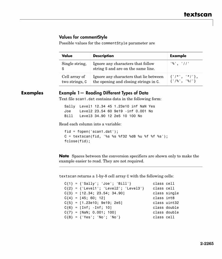
textscan
2-2265
Values for commentStylePossible values for the commentStyle parameter are
Examples Example 1— Reading Different Types of DataText file scan1.dat contains data in the following form:
Sally Level1 12.34 45 1.23e10 inf NaN YesJoe Level2 23.54 60 9e19 -inf 0.001 NoBill Level3 34.90 12 2e5 10 100 No
Read each column into a variable:
fid = fopen('scan1.dat');C = textscan(fid, '%s %s %f32 %d8 %u %f %f %s');fclose(fid);
Note Spaces between the conversion specifiers are shown only to make the example easier to read. They are not required.
textscan returns a 1-by-8 cell array C with the following cells:
C1 = 'Sally'; 'Joe'; 'Bill' class cellC2 = 'Level1'; 'Level2'; 'Level3' class cellC3 = [12.34; 23.54; 34.90] class singleC4 = [45; 60; 12] class int8C5 = [1.23e10; 9e19; 2e5] class uint32C6 = [Inf; -Inf; 10] class doubleC7 = [NaN; 0.001; 100] class doubleC8 = 'Yes'; 'No'; 'No' class cell
Value Description Example
Single string, S
Ignore any characters that follow string S and are on the same line.
'%', '//'
Cell array of two strings, C
Ignore any characters that lie between the opening and closing strings in C.
'/*', '*/','/%', '%/'

textscan
2-2266
Example 2 — Reading All But One FieldRead the file as a fixed-format file, skipping the third field:
fid = fopen('scan1.dat');C = textscan(fid, '%7c %6s %*f %d8 %u %f %f %s');fclose(fid);
textscan returns a 1-by-8 cell array C with the following cells:
C1 = ['Sally '; 'Joe '; 'Bill '] class charC2 = 'Level1'; 'Level2'; 'Level3' class cellC3 = [45; 60; 12] class int8C4 = [1.23e10; 9e19; 2e5] class uint32C5 = [Inf; -Inf; 10] class doubleC6 = [NaN; 0.001; 100] class doubleC7 = 'Yes'; 'No'; 'No' class cell
Example 3 — Reading Only the First FieldRead the first column into a cell array, skipping the rest of the line:
fid = fopen('scan1.dat');names = textscan(fid, '%s%*[^\n]');fclose(fid);
textscan returns a 1-by-1 cell array names:
size(names)ans = 1 1
The one cell contains
names1 = 'Sally'; 'Joe'; 'Bill' class cell
Example 4 — Removing a Literal String in the OutputThe second format specifier in this example, %sLevel, tells textscan to read the second field from a line in the file, but to ignore the initial string 'Level' within that field. All that is left of the field is a numeric digit. textscan assigns the next specifier, %f, to that digit, converting it to a double.
See C2 in the results:
fid = fopen('scan1.dat');

textscan
2-2267
C = textscan(fid, '%s Level%u8 %f32 %d8 %u %f %f %s');fclose(fid);
textscan returns a 1-by-8 cell array, C, with cells
C1 = 'Sally'; 'Joe'; 'Bill' class cellC2 = [1; 2; 3] class uint8C3 = [12.34; 23.54; 34.90] class singleC4 = [45; 60; 12] class int8C5 = [1.23e10; 9e19; 2e5] class uint32C6 = [Inf; -Inf; 10] class doubleC7 = [NaN; 0.001; 100] class doubleC8 = 'Yes'; 'No'; 'No' class cell
Example 5 — Using a Nondefault Delimiter and White-SpaceRead the M-file into a cell array of strings:
fid = fopen('fft.m');file = textscan(fid, '%s', 'delimiter', '\n', 'whitespace', '');fclose(fid);
textscan returns a 1-by-1 cell array, file, that contains a 37-by-1 cell array:
file = 37x1 cell
Show the first three lines of the file:
lines = file1;lines1:3, :ans = 'function [varargout] = fft(varargin)'ans = '%FFT Discrete Fourier transform.'ans = '% FFT(X) is the discrete Fourier transform (DFT) of vector X. For'
Example 6 — Using a Nondefault Empty ValueRead files with empty cells, setting the emptyvalue parameter. The file data.csv contains

textscan
2-2268
1, 2, 3, 4, , 67, 8, 9, , 11, 12
Read the file as shown here, using -Inf in empty cells:
fid = fopen('data.csv');C = textscan(fid, '%f%f%f%f%u32%f', 'delimiter', ',', ... 'emptyValue', -Inf);fclose(fid);
textscan returns a 1-by-6 cell array C with the following cells:
C1 = [1; 7] class doubleC2 = [2; 8] class doubleC3 = [3; 9] class doubleC4 = [4; NaN] class doubleC5 = [-Inf; 11] class uint32 (-Inf converted to 0)C6 = [6; 12] class double
Example 7 — Using Custom Empty Values and CommentsYou have a file data.csv that contains the lines
abc, 2, NA, 3, 4// Comment Heredef, na, 5, 6, 7
Designate what should be treated as empty values and as comments. Read in all other values from the file:
fid = fopen('data5.csv');C = textscan(fid, '%s%n%n%n%n', 'delimiter', ',', ... 'treatAsEmpty', 'NA', 'na', ... 'commentStyle', '//');fclose(fid);

textscan
2-2269
This returns the following data in cell array C:
C:ans = 'abc' 'def'ans = 2 NaNans = NaN 5ans = 3 6ans = 4 7
See Also dlmread, dlmwrite, xlswrite, fopen, importdata

textwrap
2-2270
2textwrapPurpose Return wrapped string matrix for given uicontrol
Syntax outstring = textwrap(h,instring)[outstring,position] = textwrap(h,instring)
Description outstring = textwrap(h,instring) returns a wrapped string cell array, outstring, that fits inside the uicontrol with handle h. instring is a cell array, with each cell containing a single line of text. outstring is the wrapped string matrix in cell array format. Each cell of the input string is considered a paragraph.
[outstring,position]=textwrap(h,instring) returns the recommended position of the uicontrol in the units of the uicontrol. position considers the extent of the multiline text in the x and y directions.
Example Place a text-wrapped string in a uicontrol:
pos = [10 10 100 10];h = uicontrol('Style','Text','Position',pos);string = 'This is a string for the uicontrol.',
'It should be correctly wrapped inside.';[outstring,newpos] = textwrap(h,string);pos(4) = newpos(4);set(h,'String',outstring,'Position',[pos(1),pos(2),pos(3)+10,pos(4)])
See Also uicontrol

tic, toc
2-2271
2tic, tocPurpose Stopwatch timer
Syntax ticany statements
toct = toc
Description tic starts a stopwatch timer.
toc prints the elapsed time since tic was used.
t = toc returns the elapsed time in t.
Examples This example measures how the time required to solve a linear system varies with the order of a matrix.
for n = 1:100A = rand(n,n);b = rand(n,1);ticx = A\b;t(n) = toc;
endplot(t)
See Also clock, cputime, etime, profile

timer
2-2272
2timerPurpose Construct timer object
Syntax T = timerT = timer( PropertyName1', PropertyValue1, 'PropertyName2',
PropertyValue2,...)
Description T = timer constructs a timer object with default attributes.
T = timer('PropertyName1', PropertyValue1, 'PropertyName2', PropertyValue2,...) constructs a timer object in which the given property name/value pairs are set on the object. See “Timer Object Properties” on page 2-2272 for a list of all the properties supported by the timer object.
Note that the property name/property value pairs can be in any format supported by the set function, i.e., property/value string pairs, structures, and property/value cell array pairs.
Examples This example constructs a timer object with a timer callback function handle, mycallback, and a 10 second interval.
t = timer('TimerFcn',@mycallback, 'Period', 10.0);
See Also delete, disp, get, isvalid, set, start, startat, stop, timerfind, timerfindall, wait
Timer Object Properties
The timer object supports the following properties that control its attributes. The table includes information about the data type of each property and its default value.

timer
2-2273
To view the value of the properties of a particular timer object, use the get function. To set the value of the properties of a timer object, use the set function.
Property Name Property Description Data Types, Values, and Defaults
AveragePeriod The average time between Timer-Fcn executions since the timer started.Note: Value is NaN until timer exe-cutes two timer callbacks.
Data type: Default: Read only:
doubleNaNAlways
BusyMode Action taken when a timer has to execute TimerFcn before the com-pletion of previous execution of TimerFcn.
• 'drop' — Do not execute the function.
• 'error' — Generate an error.
• 'queue' — Execute function at next opportunity.
Data type: Values:
Default:Read only:
Enumerated string'drop''error''queue''drop'While Running = 'on'
ErrorFcn Function that the timer executes when an error occurs. This func-tion executes before the StopFcn. See “Creating Timer Callback Functions” for more information.
Data type:
Default:Read only:
Text string, func-tion handle, or cell arrayNoneNever
ExecutionMode Determines how the timer object schedules timer events. See “Timer Execution Modes” for more information.
Data type: Values:
Default:Read only:
Enumerated string'singleShot''fixedDelay''fixedRate''fixedSpacing'singleShot'While Running = 'on'

timer
2-2274
InstantPeriod The time between the last two executions of TimerFcn.
Data type: Default: Read only:
doubleNaNAlways
Name User-supplied name Data type: Default:
Read only:
Text string'timer-i', where i is a number indi-cating the ith timer object cre-ated this session.To reset i to 1, exe-cute the clear classes command.Never
ObjectVisibility Provides a way for application developers to prevent end-user access to the timer objects created by their application. The timer-find function does not return an object whose ObjectVisibility property is set to 'off'. Objects that are not visible are still valid. If you have access to the object (for example, from within the M-file that created it), you can set its properties.
Data type: Values:
Default: Read only:
Enumerated string'off''on''on'Never
Period Specifies the delay, in seconds, between executions of TimerFcn.
Data type: Value:
Default:Read only:
doubleAny number > 0.001 1.0While Running = 'on'
Property Name Property Description Data Types, Values, and Defaults
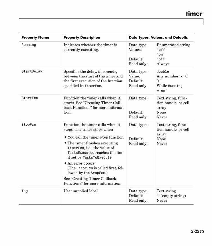
timer
2-2275
Running Indicates whether the timer is currently executing.
Data type: Values:
Default: Read only:
Enumerated string'off''on''off'Always
StartDelay Specifies the delay, in seconds, between the start of the timer and the first execution of the function specified in TimerFcn.
Data type: Value: Default: Read only:
doubleAny number >= 00While Running ='on'
StartFcn Function the timer calls when it starts. See “Creating Timer Call-back Functions” for more informa-tion.
Data type:
Default:Read only:
Text string, func-tion handle, or cell arrayNoneNever
StopFcn Function the timer calls when it stops. The timer stops when
• You call the timer stop function
• The timer finishes executing TimerFcn, i.e., the value of TasksExecuted reaches the lim-it set by TasksToExecute.
• An error occurs (The ErrorFcn is called first, fol-lowed by the StopFcn.)
See “Creating Timer Callback Functions” for more information.
Data type:
Default: Read only:
Text string, func-tion handle, or cell arrayNoneNever
Tag User supplied label Data type: Default: Read only:
Text string''(empty string)Never
Property Name Property Description Data Types, Values, and Defaults

timer
2-2276
TasksToExecute Specifies the number of times the timer should execute the function specified in the TimerFcn prop-erty.
Data type: Value: DefaultRead only:
doubleAny number > 01Never
TasksExecuted The number of times the timer has executed TimerFcn since the timer was started.
Data type: Value: Default: Read only:
doubleAny number >= 00Always
TimerFcn Timer callback function. See “Cre-ating Timer Callback Functions” for more information.
Data type:
Default:Read only:
Text string, func-tion handle, or cell arrayNoneNever
Type Identifies the object type Data type: Value:Read only:
Text string'timer'Always
UserData User-supplied data Data type: Default: Read only:
User-defined[]Never
Property Name Property Description Data Types, Values, and Defaults

timerfind
2-2277
2timerfindPurpose Find timer objects
Syntax out = timerfindout = timerfind('P1', V1, 'P2', V2,...)out = timerfind(S)out = timerfind(obj, 'P1', V1, 'P2', V2,...)
Description out = timerfind returns an array, out, of all the timer objects that exist in memory.
out = timerfind('P1', V1, 'P2', V2,...) returns an array, out, of timer objects whose property values match those passed as parameter/value pairs, P1, V1, P2, V2. Parameter/value pairs may be specified as a cell array.
out = timerfind(S) returns an array, out, of timer objects whose property values match those defined in the structure, S. The field names of S are timer object property names and the field values are the corresponding property values.
out = timerfind(obj, 'P1', V1, 'P2', V2,...) restricts the search for matching parameter/value pairs to the timer objects listed in obj. obj can be an array of timer objects.
Note When specifying parameter/value pairs, you can use any mixture of strings, structures, and cell arrays in the same call to timerfind.
Note that, for most properties, timerfind performs case-sensitive searches of property values. For example, if the value of an object's Name property is 'MyObject', timerfind will not find a match if you specify 'myobject'. Use the get function to determine the exact format of a property value. However, properties that have an enumerated list of possible values are not case sensitive. For example, timerfind will find an object with an ExecutionMode property value of 'singleShot' or 'singleshot'.
Examples These examples use timerfind to find timer objects with the specified property values.

timerfind
2-2278
t1 = timer('Tag', 'broadcastProgress', 'Period', 5);t2 = timer('Tag', 'displayProgress');out1 = timerfind('Tag', 'displayProgress')out2 = timerfind('Period', 'Tag', 5, 'broadcastProgress')
See Also get, timer, timerfindall

timerfindall
2-2279
2timerfindallPurpose Find timer objects, including invisible objects
Syntax out = timerfindallout = timerfindall('P1', V1, 'P2', V2,...)out = timerfindall(S)out = timerfindall(obj, 'P1', V1, 'P2', V2,...)
Description out = timerfindall returns an array, out, containing all the timer objects that exist in memory, regardless of the value of the object's ObjectVisibility property.
out = timerfindall('P1', V1, 'P2', V2,...) returns an array, out, of timer objects whose property values match those passed as parameter/value pairs, P1, V1, P2, V2. Parameter/value pairs may be specified as a cell array.
out = timerfindall(S) returns an array, out, of timer objects whose property values match those defined in the structure, S. The field names of S are timer object property names and the field values are the corresponding property values.
out = timerfindall(obj, 'P1', V1, 'P2', V2,...) restricts the search for matching parameter/value pairs to the timer objects listed in obj. obj can be an array of timer objects.
Note When specifying parameter/value pairs, you can use any mixture of strings, structures, and cell arrays in the same call to timerfindall.
Note that, for most properties, timerfindall performs case-sensitive searches of property values. For example, if the value of an object's Name property is 'MyObject', timerfindall will not find a match if you specify 'myobject'. Use the get function to determine the exact format of a property value. However, properties that have an enumerated list of possible values are not case sensitive. For example, timerfindall will find an object with an ExecutionMode property value of 'singleShot' or 'singleshot'.
Examples Create several timer objects.

timerfindall
2-2280
t1 = timer;t2 = timer;t3 = timer;
Set the ObjectVisibility property of one of the objects to 'off'.
t2.ObjectVisibility = 'off';
Use timerfind to get a listing of all the timer objects in memory. Note that the listing does not include the timer object (timer-2) whose ObjectVisibility property is set to 'off'.
timerfind
Timer Object Array
Index: ExecutionMode: Period: TimerFcn: Name: 1 singleShot 1 '' timer-1 2 singleShot 1 '' timer-3
Use timerfindall to get a listing of all the timer objects in memory. This listing includes the timer object whose ObjectVisibility property is set to 'off'.
timerfindall
Timer Object Array
Index: ExecutionMode: Period: TimerFcn: Name: 1 singleShot 1 '' timer-1 2 singleShot 1 '' timer-2
3 singleShot 1 '' timer-3
See Also get, timer, timerfind

title
2-2281
2titlePurpose Add title to current axes
Syntax title('string')title(fname)title(...,'PropertyName',PropertyValue,...)h = title(...)
Description Each axes graphics object can have one title. The title is located at the top and in the center of the axes.
title('string') outputs the string at the top and in the center of the current axes.
title(fname) evaluates the function that returns a string and displays the string at the top and in the center of the current axes.
title(...,'PropertyName',PropertyValue,...) specifies property name and property value pairs for the text graphics object that title creates.
h = title(...) returns the handle to the text object used as the title.
Examples Display today’s date in the current axes:
title(date)
Include a variable’s value in a title:
f = 70;c = (f 32)/1.8;title(['Temperature is ',num2str(c),'C'])
Include a variable’s value in a title and set the color of the title to yellow:
n = 3;title(['Case number #',int2str(n)],'Color','y')
Include Greek symbols in a title:
title('\ite^\omega\tau = cos(\omega\tau) + isin(\omega\tau)')
Include a superscript character in a title:
title('\alpha^2')

title
2-2282
Include a subscript character in a title:
title('X_1')
The text object String property lists the available symbols.
Create a multiline title using a multiline cell array.
title('First line';'Second line')
Remarks title sets the Title property of the current axes graphics object to a new text graphics object. See the text String property for more information.
See Also gtext, int2str, num2str, text, xlabel, ylabel, zlabel
“Annotating Plots” for related functions
Adding Titles to Graphs for more information on ways to add titles

todatenum
2-2283
2todatenum Purpose Convert CDF epoch object to MATLAB datenum
Syntax n = todatenum(ep_obj)
Description n = todatenum(obj) converts the CDF epoch object ep_obj into a MATLAB serial date number. Note that a CDF epoch is the number of milliseconds since 01-Jan-0000 whereas a MATLAB datenum is the number of days since 00-Jan-0000.
Examples Construct a CDF epoch object from a date string, and then convert the object back into a MATLAB date string:
dstr = datestr(today)dstr = 08-Oct-2003
obj = cdfepoch(dstr)obj = cdfepoch object: 08-Oct-2003 00:00:00
dstr2 = datestr(todatenum(obj))dstr2 = 08-Oct-2003
See Also cdfepoch, cdfinfo, cdfread, cdfwrite, datenum

toeplitz
2-2284
2toeplitzPurpose Toeplitz matrix
Syntax T = toeplitz(c,r)T = toeplitz(r)
Description A Toeplitz matrix is defined by one row and one column. A symmetric Toeplitz matrix is defined by just one row. toeplitz generates Toeplitz matrices given just the row or row and column description.
T = toeplitz(c,r) returns a nonsymmetric Toeplitz matrix T having c as its first column and r as its first row. If the first elements of c and r are different, a message is printed and the column element is used.
T = toeplitz(r) returns the symmetric or Hermitian Toeplitz matrix formed from vector r, where r defines the first row of the matrix.
Examples A Toeplitz matrix with diagonal disagreement is
c = [1 2 3 4 5];r = [1.5 2.5 3.5 4.5 5.5];toeplitz(c,r)Column wins diagonal conflict:ans =
1.000 2.500 3.500 4.500 5.5002.000 1.000 2.500 3.500 4.5003.000 2.000 1.000 2.500 3.5004.000 3.000 2.000 1.000 2.5005.000 4.000 3.000 2.000 1.000
See Also hankel

trace
2-2285
2tracePurpose Sum of diagonal elements
Syntax b = trace(A)
Description b = trace(A) is the sum of the diagonal elements of the matrix A.
Algorithm trace is a single-statement M-file.
t = sum(diag(A));
See Also det, eig

trapz
2-2286
2trapzPurpose Trapezoidal numerical integration
Syntax Z = trapz(Y)Z = trapz(X,Y)Z = trapz(...,dim)
Description Z = trapz(Y) computes an approximation of the integral of Y via the trapezoidal method (with unit spacing). To compute the integral for spacing other than one, multiply Z by the spacing increment.
If Y is a vector, trapz(Y) is the integral of Y.
If Y is a matrix,trapz(Y) is a row vector with the integral over each column.
If Y is a multidimensional array, trapz(Y) works across the first nonsingleton dimension.
Z = trapz(X,Y) computes the integral of Y with respect to X using trapezoidal integration.
If X is a column vector and Y an array whose first nonsingleton dimension is length(X), trapz(X,Y) operates across this dimension.
Z = trapz(...,dim) integrates across the dimension of Y specified by scalar dim. The length of X, if given, must be the same as size(Y,dim).
Examples The exact value of is 2.
To approximate this numerically on a uniformly spaced grid, use
X = 0:pi/100:pi;Y = sin(x);
Then both
Z = trapz(X,Y)
and
Z = pi/100*trapz(Y)
produce

trapz
2-2287
Z =1.9998
A nonuniformly spaced example is generated by
X = sort(rand(1,101)*pi);Y = sin(X);Z = trapz(X,Y);
The result is not as accurate as the uniformly spaced grid. One random sample produced
Z =1.9984
See Also cumsum, cumtrapz

treelayout
2-2288
2treelayoutPurpose Lay out tree or forest
Syntax [x,y] = treelayout(parent,post)[x,y,h,s] = treelayout(parent,post)
Description [x,y] = treelayout(parent,post) lays out a tree or a forest. parent is the vector of parent pointers, with 0 for a root. post is an optional postorder permutation on the tree nodes. If you omit post, treelayout computes it. x and y are vectors of coordinates in the unit square at which to lay out the nodes of the tree to make a nice picture.
[x,y,h,s] = treelayout(parent,post) also returns the height of the tree h and the number of vertices s in the top-level separator.
See Also etree, treeplot, etreeplot, symbfact

treeplot
2-2289
2treeplotPurpose Plot picture of tree
Syntax treeplot(p)treeplot(p,nodeSpec,edgeSpec)
Description treeplot(p) plots a picture of a tree given a vector of parent pointers, with p(i) = 0 for a root.
treeplot(p,nodeSpec,edgeSpec) allows optional parameters nodeSpec and edgeSpec to set the node or edge color, marker, and linestyle. Use '' to omit one or both.
See Also etree, etreeplot, treelayout

tril
2-2290
2trilPurpose Lower triangular part of a matrix
Syntax L = tril(X)L = tril(X,k)
Description L = tril(X) returns the lower triangular part of X.
L = tril(X,k) returns the elements on and below the kth diagonal of X. k = 0 is the main diagonal, k > 0 is above the main diagonal, and k < 0 is below the main diagonal.
Examples tril(ones(4,4),-1)
ans =
0 0 0 01 0 0 01 1 0 01 1 1 0
See Also diag, triu

trimesh
2-2291
2trimeshPurpose Triangular mesh plot
Syntax trimesh(Tri,X,Y,Z)trimesh(Tri,X,Y,Z,C)trimesh(...'PropertyName',PropertyValue...)h = trimesh(...)
Description trimesh(Tri,X,Y,Z) displays triangles defined in the m-by-3 face matrix Tri as a mesh. Each row of Tri defines a single triangular face by indexing into the vectors or matrices that contain the X, Y, and Z vertices.
trimesh(Tri,X,Y,Z,C) specifies color defined by C in the same manner as the surf function. MATLAB performs a linear transformation on this data to obtain colors from the current colormap.
trimesh(...'PropertyName',PropertyValue...) specifies additional patch property names and values for the patch graphics object created by the function.
h = trimesh(...) returns a handle to a patch graphics object.
Example Create vertex vectors and a face matrix, then create a triangular mesh plot.
x = rand(1,50);y = rand(1,50);z = peaks(6*x 3,6*x 3);tri = delaunay(x,y);trimesh(tri,x,y,z)
See Also patch, tetramesh, triplot, trisurf, delaunay
“Creating Surfaces and Meshes” for related functions

triplequad
2-2292
2triplequadPurpose Numerically evaluate triple integral
Syntax triplequad(fun,xmin,xmax,ymin,ymax,zmin,zmax)triplequad(fun,xmin,xmax,ymin,ymax,zmin,zmax,tol)triplequad(fun,xmin,xmax,ymin,ymax,zmin,zmax,tol,method)
Description triplequad(fun,xmin,xmax,ymin,ymax,zmin,zmax) evaluates the triple integral fun(x,y,z) over the three dimensional rectangular region xmin <= x <= xmax, ymin <= y <= ymax, zmin <= z <= zmax. fun is a function handle for either an M-file function or an anonymous function. fun(x,y,z) must accept a vector x and scalars y and z, and return a vector of values of the integrand.
Parameterizing Functions Called by Function Functions, in the online MATLAB documentation, explains how to provide addition parameters to the function fun, if necessary.
triplequad(fun,xmin,xmax,ymin,ymax,zmin,zmax,tol) uses a tolerance tol instead of the default, which is 1.0e-6.
triplequad(fun,xmin,xmax,ymin,ymax,zmin,zmax,tol,method) uses the quadrature function specified as method, instead of the default quad. Valid values for method are @quadl or the function handle of a user-defined quadrature method that has the same calling sequence as quad and quadl.
Examples Pass M-file function handle @integrnd to triplequad:
Q = triplequad(@integrnd,0,pi,0,1,-1,1);
where the M-file integrnd.m is
function f = integrnd(x,y,z)f = y*sin(x)+z*cos(x);
Pass anonymous function handle F to triplequad:
F = @(x,y,z)y*sin(x)+z*cos(x);Q = triplequad(F,0,pi,0,1,-1,1);
This example integrates y*sin(x)+z*cos(x) over the region 0 <= x <= pi, 0 <= y <= 1, -1 <= z <= 1. Note that the integrand can be evaluated with a vector x and scalars y and z.

triplequad
2-2293
See Also dblquad, quad, quadl, @ (function handle), anonymous functions

triplot
2-2294
2triplotPurpose 2-D triangular plot
Syntax triplot(TRI,x,y)triplot(TRI,x,y,color)h = triplot(...)triplot(...,'param','value','param','value'...)
Description triplot(TRI,x,y) displays the triangles defined in the m-by-3 matrix TRI. A row of TRI contains indices into the vectors x and y that define a single triangle. The default line color is blue.
triplot(TRI,x,y,color) uses the string color as the line color. color can also be a line specification. See ColorSpec for a list of valid color strings. See LineSpec for information about line specifications.
h = triplot(...) returns a vector of handles to the displayed triangles.
triplot(...,'param','value','param','value'...) allows additional line property name/property value pairs to be used when creating the plot. See Line Properties for information about the available properties.
Examples This code plots the Delaunay triangulation for 10 randomly generated points.
rand('state',7);x = rand(1,10); y = rand(1,10); TRI = delaunay(x,y);triplot(TRI,x,y,'red')
See Also ColorSpec, delaunay, line, Line Properties, LineSpec, plot, trimesh, trisurf

trisurf
2-2295
2trisurfPurpose Triangular surface plot
Syntax trisurf(Tri,X,Y,Z)trisurf(Tri,X,Y,Z,C)trisurf(...'PropertyName',PropertyValue...)h = trisurf(...)
Description trisurf(Tri,X,Y,Z) displays triangles defined in the m-by-3 face matrix Tri as a surface. Each row of Tri defines a single triangular face by indexing into the vectors or matrices that contain the X, Y, and Z vertices.
trisurf(Tri,X,Y,Z,C) specifies color defined by C in the same manner as the surf function. MATLAB performs a linear transformation on this data to obtain colors from the current colormap.
trisurf(...'PropertyName',PropertyValue...) specifies additional patch property names and values for the patch graphics object created by the function.
h = trisurf(...) returns a patch handle.
Example Create vertex vectors and a face matrix, then create a triangular surface plot.
x = rand(1,50);y = rand(1,50);z = peaks(6*x 3,6*x 3);tri = delaunay(x,y);trisurf(tri,x,y,z)
See Also patch, surf, tetramesh, trimesh, triplot, delaunay
“Creating Surfaces and Meshes” for related functions

triu
2-2296
2triuPurpose Upper triangular part of a matrix
Syntax U = triu(X)U = triu(X,k)
Description U = triu(X) returns the upper triangular part of X.
U = triu(X,k) returns the element on and above the kth diagonal of X. k = 0 is the main diagonal, k > 0 is above the main diagonal, and k < 0 is below the main diagonal.
Examples triu(ones(4,4),-1)
ans =
1 1 1 11 1 1 10 1 1 10 0 1 1
See Also diag, tril

true
2-2297
2truePurpose True array
Syntax truetrue(n)true(m, n)true(m, n, p, ...)true(size(A))
Description true is shorthand for logical 1.
true(n) is an n-by-n matrix of logical ones.
true(m, n) or true([m, n]) is an m-by-n matrix of logical ones.
true(m, n, p, ...) or true([m n p ...]) is an m-by-n-by-p-by-... array of logical ones.
true(size(A)) is an array of logical ones that is the same size as array A.
Remarks true(n) is much faster and more memory efficient than logical(ones(n)).
See Also false, logical

try
2-2298
2tryPurpose Begin try block
Description The general form of a try statement is
try, statement, ..., statement, catch, statement, ..., statement, end
Normally, only the statements between the try and catch are executed. However, if an error occurs during execution of any of the statements, the error is captured into lasterr, and the statements between the catch and end are executed. If an error occurs within the catch statements, execution stops unless caught by another try...catch block. The error string produced by a failed try block can be obtained with lasterr.
See Also catch, end, lasterr, eval, evalin

tsearch
2-2299
2tsearchPurpose Search for enclosing Delaunay triangle
Syntax T = tsearch(x,y,TRI,xi,yi)
Description T = tsearch(x,y,TRI,xi,yi) returns an index into the rows of TRI for each point in xi, yi. The tsearch command returns NaN for all points outside the convex hull. Requires a triangulation TRI of the points x,y obtained from delaunay.
See Also delaunay, delaunayn, dsearch, tsearchn

tsearchn
2-2300
2tsearchnPurpose N-dimensional closest simplex search
Syntax t = tsearchn(X,TES,XI)[t,P] = tsearchn(X,TES,XI)
Description t = tsearchn(X,TES,XI) returns the indices t of the enclosing simplex of the Delaunay tessellation TES for each point in XI. X is an m-by-n matrix, representing m points in N-dimensional space. XI is a p-by-n matrix, representing p points in N-dimensional space. tsearchn returns NaN for all points outside the convex hull of X. tsearchn requires a tessellation TES of the points X obtained from delaunayn.
[t,P] = tsearchn(X,TES,XI) also returns the barycentric coordinate P of XI in the simplex TES. P is a p-by-n+1 matrix. Each row of P is the Barencentric coordinate of the corresponding point in XI. It is useful for interpolation.
See Also delaunayn, griddatan, tsearch

uibuttongroup
2-2301
2uibuttongroupPurpose Container object to exclusively manage radio buttons and toggle buttons
Syntax uibuttongroup('PropertyName1,Value1,'PropertyName2',Value2,...)handle = uibuttongroup(...)
Description A uibuttongroup groups components and manages exclusive selection behavior for radio buttons and toggle buttons that it contains. It can also contain other user interface controls, axes, uipanels, and uibuttongroups. It cannot contain ActiveX controls.
uibuttongroup('PropertyName1',Value1,'PropertyName2',Value2,...)creates a visible container component in the current figure window. This component manages exclusive selection behavior for uicontrols of style radiobutton and togglebutton.
Use the Parent property to specify the parent as a figure, uipanel, or uibuttongroup. If you do not specify a parent, uibuttongroup adds the button group to the current figure. If no figure exists, one is created.
A uibuttongroup object can have axes, uicontrol, uipanel, and uibuttongroup objects as children. However, only uicontrols of style radiobutton and togglebutton are managed by the component.
For the children of a uibuttongroup object, the Position property is interpreted relative to the button group. If you move the button group, the children automatically move with it and maintain their positions in the button group.
Note Include code for uicontrols of style radiobutton and togglebutton that are managed by a uibuttongroup in the SelectionChangeFcn callback function, not in the individual uicontrol Callback functions. uibuttongroup overwrites the Callback properties of radio buttons and toggle buttons that it manages. See the SelectionChangeFcn property and the example on this reference page for more information.
handle = uibuttongroup(...) creates a uibuttongroup object and returns a handle to it in handle.

uibuttongroup
2-2302
After creating a uibuttongroup, you can set and query its property values using set and get. Run get(handle) to see a list of properties and their current values. Run set(handle) to see a list of object properties you can set and their legal values.
Properties This table lists all properties useful to uibuttongroup objects, grouping them by function. Each property name acts as a link to a description of the property. Curly braces denote the default value, if any.
Property Name Description Property Value
Controlling Style and Appearance
BackgroundColor Color of the uibuttongroup background
ColorSpec. Default is the same as the default uicontrol background.
BorderType Type of border around the uibuttongroup area.
[ none | etchedin | etchedout | beveledin | beveledout | line ]
BorderWidth Width in pixels of the button group border.
Integer. Default is 1.
Clipping Clipping of child axes, uipanels, and uibuttongroups to the uibuttongroup. Does not affect child uicontrols.
[on|off]
ForegroundColor Title font color and color of 2-D border line
ColorSpec. Default is [0 0 0] (black).
HighlightColor 3-D frame highlight color ColorSpec. Default is [1 1 1] (white).
SelectionHighlight Object highlighted when selected
[on|off]
ShadowColor 3-D frame shadow color ColorSpec. Default is [.5 .5 .5] (grey).

uibuttongroup
2-2303
Visible Uibuttongroup visibility. Note: Controls the Visible property of child axes, uipanels, and uibuttongroups. Does not affect child uicontrols.
[on|off]
General Information About the Object
Children All children of the uibuttongroup object
Vector of handles
Parent uibuttongroup object’s parent
Scalar figure, uipanel, or uibuttongroup handle
Selected Whether object is selected [on|off]
SelectedObject Currently selected radio button or toggle button
Scalar handle. Default is the first uicontrol radio button or toggle button added. Set to [] for no selection.
Tag User-specified object identifier
String
UserData User-specified data Matrix
Controlling the Object Position
Position Button group position relative to parent figure, panel, or button group
Position spec [x y w h]. Default is [0 0 1 1]
Units Units used to interpret the position vector
[inches|centimeters|normalized|points|pixels|characters]
Property Name Description Property Value

uibuttongroup
2-2304
Controlling Fonts and Labels
FontAngle Title font angle [normal|italic|oblique]
FontName Title font name String. Default is system dependent.
FontSize Title font size Integer. Default is system dependent.
FontUnits Title font units [inches|centimeters|normalized|points|pixels]
FontWeight Title font weight [light|normal|demi|bold]
Title Title string String
TitlePosition Location of title string in relation to the button group
[lefttop|centertop|righttop|leftbottom|centerbottom|rightbottom]
Controlling Callback Routine Execution
BusyAction Interruption of other callback routines
[queue|cancel]
ButtonDownFcn Button-press callback routine
String or function handle
CreateFcn Callback routine executed during object creation
String or function handle
DeleteFcn Callback routine executed during object deletion
String or function handle
Interruptible Callback routine interruption mode
[on|off]
Property Name Description Property Value

uibuttongroup
2-2305
Examples This example creates a uibuttongroup with three radiobuttons. It manages the radiobuttons with the SelectionChangeFcn callback, selcbk.
When you select a new radio button, selcbk displays the uibuttongroup handle on one line, the EventName, OldValue, and NewValue fields of the event data structure on a second line, and the value of the SelectedObject property on a third line.
h = uibuttongroup('visible','off','Position',[0 0 .2 1]);u0 = uicontrol('Style','Radio','String','Option 1',... 'pos',[10 350 100 30],'parent',h,'HandleVisibility','off');u1 = uicontrol('Style','Radio','String','Option 2',... 'pos',[10 250 100 30],'parent',h,'HandleVisibility','off');u2 = uicontrol('Style','Radio','String','Option 3',... 'pos',[10 150 100 30],'parent',h,'HandleVisibility','off');set(h,'SelectionChangeFcn',@selcbk);set(h,'SelectedObject',[]); % No selectionset(h,'Visible','on');
ResizeFcn User-specified resize routine
String or function handle
SelectionChangeFcn Callback routine executed when the selected radio button or toggle button changes.
String or function handle
UIContextMenu Associates a uicontextmenu with the uibuttongroup
Scalar handle
Controlling Access to Objects
HandleVisibility Handle accessibility from commandline and GUIs
[on|callback|off]
HitTest Selectable by mouse click [on|off]
Property Name Description Property Value

uibuttongroup
2-2306
For the SelectionChangeFcn callback, selcbk, the source and event data structure arguments are available only if selcbk is called using a function handle. See SelectionChangeFcn for more information.
function selcbk(source,eventdata)disp(source);disp([eventdata.EventName,' ',... get(eventdata.OldValue,'String'),' ', ... get(eventdata.NewValue,'String')]);disp(get(get(source,'SelectedObject'),'String'));
If you click Option 2 with no option selected, the SelectionChangeFcn callback, selcbk, displays:
3.0011
SelectionChanged Option 2Option 2

uibuttongroup
2-2307
If you then click Option 1, the SelectionChangeFcn callback, selcbk, displays:
3.0011
SelectionChanged Option 2 Option 1Option 1
See Also uicontrol, uipanel

Uibuttongroup Properties
2-2308
2Uibuttongroup PropertiesModifying Properties
You can set and query graphics object properties in two ways:
• The Property Inspector is an interactive tool that enables you to see and change object property values. The Property inspector is available from GUIDE, or use the inspect function at the command line.
• The set and get functions enable you to set and query the values of properties.
Uibuttongroup takes its default property values from uipanel. To set a uibuttongroup default property value, set the default for the corresponding uipanel property. Note that you can set no default values for the uibuttongroup SelectedObject and SelectionChangeFcn properties.
For more information about changing the default value of a property see Setting Default Property Values. For an example, see the CreateFcn property.
Uibuttongroup Properties
This section describes all properties useful to uibuttongroup objects and lists valid values. Curly braces enclose default values.
Property Name Description
BackgroundColor Color of the uibuttongroup background
BorderType Type of border around the uibuttongroup area.
BorderWidth Width of the button group border in pixels.
BusyAction Interruption of other callback routines
ButtonDownFcn Button-press callback routine
Children All children of the uibuttongroup
Clipping Clipping of child axes, uipanels, and uibuttongroups to the uibuttongroup. Does not affect child uicontrols.
CreateFcn Callback routine executed during object creation
DeleteFcn Callback routine executed during object deletion
FontAngle Title font angle

Uibuttongroup Properties
2-2309
FontName Title font name
FontSize Title font size
FontUnits Title font units
FontWeight Title font weight
ForegroundColor Title font color and color of 2-D border line
HandleVisibility Handle accessibility from command line and GUIs
HighlightColor 3-D frame highlight color
HitTest Selectable by mouse click
Interruptible Callback routine interruption mode
Parent uibuttongroup object’s parent
Position Uibuttongroup position relative to parent figure, uipanel, or uibuttongroup
ResizeFcn User-specified resize routine
Selected Whether object is selected
SelectedObject Currently selected uicontrol of style radiobutton or togglebutton
SelectionChangeFcn Callback routine executed when the selected radio button or toggle button changes.
SelectionHighlight Object highlighted when selected
ShadowColor 3-D frame shadow color
Tag User-specified object identifier
Title Title string
TitlePosition Location of title string in relation to the button group
UIContextMenu Associates uicontext menu with the uibuttongroup
Property Name Description

Uibuttongroup Properties
2-2310
BackgroundColor ColorSpec
Color of the uibuttongroup background. A three-element RGB vector or one of the MATLAB predefined names, specifying the background color. See the ColorSpec reference page for more information on specifying color.
BorderType none | etchedin | etchedout |beveledin | beveledout | line
Border of the uibuttongroup area. Used to define the button group area graphically. Etched and beveled borders provide a 3-D look. Use the HighlightColor and ShadowColor properties to specify the border color of etched and beveled borders. A line border is 2-D. Use the ForegroundColor property to specify its color.
BorderWidth integer
Width of the button group border. The width of the button group borders in pixels. The default border width is 1 pixel. 3-D borders wider than 3 may not appear correctly at the corners.
BusyAction cancel | queue
Callback routine interruption. If a callback is executing and the user triggers an event (such as a mouse click) on an object for which a callback is defined, the callback associated with the new event uses the value of BusyAction to decide whether or not to attempt to interrupt the executing callback.
• If the value is cancel, the event is discarded and the second callback does not execute.
• If the value is queue, and the Interruptible property of the first callback is on, the second callback is added to the event queue and executes in its turn after the first callback finishes execution.
Units Units used to interpret the position vector
UserData User-specified data
Visible Uibuttongroup visibility. Note: Controls the Visible property of child axes, uipanels, and uibuttongroups. Does not affect child uicontrols.
Property Name Description

Uibuttongroup Properties
2-2311
Note If the interrupting callback is a DeleteFcn or CreateFcn callback or a figure’s CloseRequest or ResizeFcn callback, it interrupts an executing callback regardless of the value of that object’s Interruptible property. See the Interruptible property for information about controlling a callback’s interruptibility.
ButtonDownFcn string or function handle
Button-press callback routine. A callback routine that executes when you press a mouse button while the pointer is in a 5-pixel wide border around the uibuttongroup. This is useful for implementing actions to interactively modify object properties, such as size and position, when they are clicked on (using the selectmoveresize function, for example).
If you define this routine as a string, the string can be a valid MATLAB expression or the name of an M-file. The expression executes in the MATLAB workspace.
Children vector of handles
Children of the uibuttongroup. A vector containing the handles of all children of the uibuttongroup. Although a uibuttongroup manages only uicontrols of style radiobutton and togglebutton, its children can be axes, uipanels, uibuttongroups, and other uicontrols. You can use this property to reorder the children.
Clipping on | off
Clipping mode. By default, MATLAB clips a uibuttongroup’s child axes, uipanels, and uibuttongroups to the uibuttongroup rectangle. If you set Clipping to off, the axis, uipanel, or uibuttongroup is displayed outside the button group rectangle. This property does not affect child uicontrols which, by default, can display outside the button group rectangle.
CreateFcn string or function handle
Callback routine executed during object creation. The specified function executes when MATLAB creates a uibuttongroup object. MATLAB sets all property values for the uibuttongroup before executing the CreateFcn callback so these values are available to the callback. Within the function, use gcbo to get the handle of the uibuttongroup being created.

Uibuttongroup Properties
2-2312
Setting this property on an existing uibuttongroup object has no effect.
To define a default CreateFcn callback for all new uibuttongroups you must define the same default for all uipanels. This default applies unless you override it by specifying a different CreateFcn callback when you call uibuttongroup. For example, the code
set(0,'DefaultUipanelCreateFcn','set(gcbo,... ''FontName'',''arial'',''FontSize'',12)')
creates a default CreateFcn callback that runs whenever you create a new panel or button group. It sets the default font name and font size of the uipanel or uibuttongroup title.
To override this default and create a button group whose FontName and FontSize properties are set to different values, call uibuttongroup with code similar to
hpt = uibuttongroup(...,'CreateFcn','set(gcbo,...''FontName'',''times'',''FontSize'',14)')
Note To override a default CreateFcn callback you must provide a new callback and not just provide different values for the specified properties. This is because the CreateFcn callback runs after the property values are set, and can override property values you have set explicitly in the uibuttongroup call. In the example above, if instead of redefining the CreateFcn property for this uibuttongroup, you had explicitly set FontSize to 14, the default CreateFcn callback would have set FontSize back to the system dependent default.
See Function Handle Callbacks for information on how to use function handles to define a callback function.
DeleteFcn string or function handle
Callback routine executed during object deletion. A callback routine that executes when you delete the uibuttongroup object (e.g., when you issue a delete command or clear the figure containing the uibuttongroup). MATLAB executes the routine before destroying the object's properties so these values are available to the callback routine. The handle of the object whose DeleteFcn

Uibuttongroup Properties
2-2313
is being executed is accessible only through the root CallbackObject property, which you can query using gcbo.
FontAngle normal | italic | oblique
Character slant used in the Title. MATLAB uses this property to select a font from those available on your particular system. Setting this property to italic or oblique selects a slanted version of the font, when it is available on your system.
FontName string
Font family used in the Title. The name of the font in which to display the Title. To display and print properly, this must be a font that your system supports. The default font is system dependent. To eliminate the need to hard code the name of a fixed-width font, which may not display text properly on systems that do not use ASCII character encoding (such as in Japan), set FontName to the string FixedWidth. This string value is case insensitive.
set(uicontrol_handle,'FontName','FixedWidth')
This then uses the value of the root FixedWidthFontName property, which can be set to the appropriate value for a locale from startup.m in the end user's environment. Setting the root FixedWidthFontName property causes an immediate update of the display to use the new font.
FontSize integer
Title font size. A number specifying the size of the font in which to display the Title, in units determined by the FontUnits property. The default size is system dependent.
FontUnits inches | centimeters | normalized | points |pixels
Title font size units. Normalized units interpret FontSize as a fraction of the height of the uibuttongroup. When you resize the uibuttongroup, MATLAB modifies the screen FontSize accordingly. pixels, inches, centimeters, and points are absolute units (1 point = 1/72 inch).
FontWeight light | normal | demi | bold
Weight of characters in the title. MATLAB uses this property to select a font from those available on your particular system. Setting this property to bold causes MATLAB to use a bold version of the font, when it is available on your system.

Uibuttongroup Properties
2-2314
ForegroundColor ColorSpec
Color used for title font and 2-D border line. A three-element RGB vector or one of the MATLAB predefined names, specifying the font or line color. See the ColorSpec reference page for more information on specifying color.
HandleVisibility on | callback | off
Control access to object’s handle. This property determines when an object’s handle is visible in its parent’s list of children. When a handle is not visible in its parent’s list of children, it is not returned by functions that obtain handles by searching the object hierarchy or querying handle properties. This includes get, findobj, gca, gcf, gco, newplot, cla, clf, and close. Neither is the handle visible in the parent figure’s CurrentObject property. Handles that are hidden are still valid. If you know an object’s handle, you can set and get its properties, and pass it to any function that operates on handles.
• Handles are always visible when HandleVisibility is on.
• Setting HandleVisibility to callback causes handles to be visible from within callback routines or functions invoked by callback routines, but not from within functions invoked from the command line. This provides a means to protect GUIs from command-line users, while allowing callback routines to have complete access to object handles.
• Setting HandleVisibility to off makes handles invisible at all times. This may be necessary when a callback routine invokes a function that might potentially damage the GUI (such as evaluating a user-typed string), and so temporarily hides its own handles during the execution of that function.
Note Uicontrols of style radiobutton and togglebutton that are managed by a uibuttongroup should not be accessed outside the button group. Set the HandleVisibility of such radio buttons and toggle buttons to off or callback to prevent inadvertent access.
You can set the root ShowHiddenHandles property to on to make all handles visible, regardless of their HandleVisibility settings. This does not affect the values of the HandleVisibility properties.

Uibuttongroup Properties
2-2315
HighlightColor ColorSpec
3-D frame highlight color. A three-element RGB vector or one of the MATLAB predefined names, specifying the highlight color. See the ColorSpec reference page for more information on specifying color.
HitTest on | off
Selectable by mouse click. HitTest determines if the figure can become the current object (as returned by the gco command and the figure CurrentObject property) as a result of a mouse click on the figure. If HitTest is off, clicking the figure sets the CurrentObject to the empty matrix.
Interruptible on | off
Callback routine interruption mode. If a callback is executing and the user triggers an event (such as a mouse click) on an object for which a callback is defined, that callback attempts to interrupt the first callback. MATLAB processes the callbacks according to these factors:
• The Interruptible property of the object whose callback is executing
• Whether the executing callback contains drawnow, figure, getframe, pause, or waitfor statements
• The BusyAction property of the object whose callback is waiting to execute
If the Interruptible property of the object whose callback is executing is on (the default), the callback can be interrupted. Whenever the callback calls one of the drawnow, figure, getframe, pause, or waitfor functions, the function processes any events in the event queue, including the waiting callback, before performing its defined task.
If the Interruptible property of the object whose callback is executing is off, the callback cannot be interrupted (except by certain callbacks; see the note below). The BusyAction property of the object whose callback is waiting to execute determines what happens to the waiting callback.
Note If the interrupting callback is a DeleteFcn or CreateFcn callback or a figure’s CloseRequest or ResizeFcn callback, it interrupts an executing callback regardless of the value of that object’s Interruptible property. The interrupting callback starts execution at the next drawnow, figure, getframe, pause, or waitfor statement. A figure’s WindowButtonDownFcn callback

Uibuttongroup Properties
2-2316
routine, or an object’s ButtonDownFcn or Callback routine are processed according to the rules described above.
Parent handle
Uibuttongroup parent. The handle of the uibuttongroup’s parent figure, uipanel, or uibuttongroup. You can move a uibuttongroup object to another figure, uipanel, or uibuttongroup by setting this property to the handle of the new parent.
Position position rectangle
Size and location of uibuttongroup relative to parent. The rectangle defined by this property specifies the size and location of the button group within the parent figure window, uipanel, or uibuttongroup. Specify Position as
[left bottom width height]
left and bottom are the distance from the lower-left corner of the parent object to the lower-left corner of the uibuttongroup object. width and height are the dimensions of the uibuttongroup rectangle, including the title. All measurements are in units specified by the Units property.
ResizeFcn string or function handle
Resize callback routine. MATLAB executes this callback routine whenever a user resizes the uibuttongroup and the figure Resize property is set to on, or in GUIDE, the Resize behavior option is set to Other. You can query the uibuttongroup Position property to determine its new size and position. During execution of the callback routine, the handle to the figure being resized is accessible only through the root CallbackObject property, which you can query using gcbo.
You can use ResizeFcn to maintain a GUI layout that is not directly supported by the MATLAB Position/Units paradigm.
See Function Handle Callbacks for information on how to use function handles to define the callback function.
See Resize Behavior for information on creating resize functions using GUIDE.

Uibuttongroup Properties
2-2317
Selected on | off (read only)
Is object selected? This property indicates whether the figure is selected. When this property is on, MATLAB displays selection handles if the SelectionHighlight property is also on. You can, for example, define the ButtonDownFcn to set this property, allowing users to select the object with the mouse.
SelectedObject scalar handle
Currently selected radio button or toggle button uicontrol in the managed group of components. Use this property to determine the currently selected component or to initialize selection of one of the radio buttons or toggle buttons. By default, SelectedObject is set to the first uicontrol radio button or toggle button that is added. Set it to [] if you want no selection. Note that SelectionChangeFcn does not execute when this property is set by the user.
SelectionChangeFcn string or function handle
Callback routine executed when the selected radio button or toggle button changes. If this routine is called as a function handle, uibuttongroup passes it two arguments. The first argument is the handle of the uibuttongroup. The second argument is an event data structure that contains the fields shown in the following table.
Include code for uicontrol radio buttons and toggle buttons that are managed by a uibuttongroup in the SelectionChangeFcn callback function, not in the individual uicontrol Callback functions. uibuttongroup overwrites the Callback properties of radio buttons and toggle buttons that it manages.
Event Data Structure Field
Description
EventName 'SelectionChanged'
OldValue Handle of the object selected before this event. [] if none was selected.
NewValue Handle of the currently selected object.
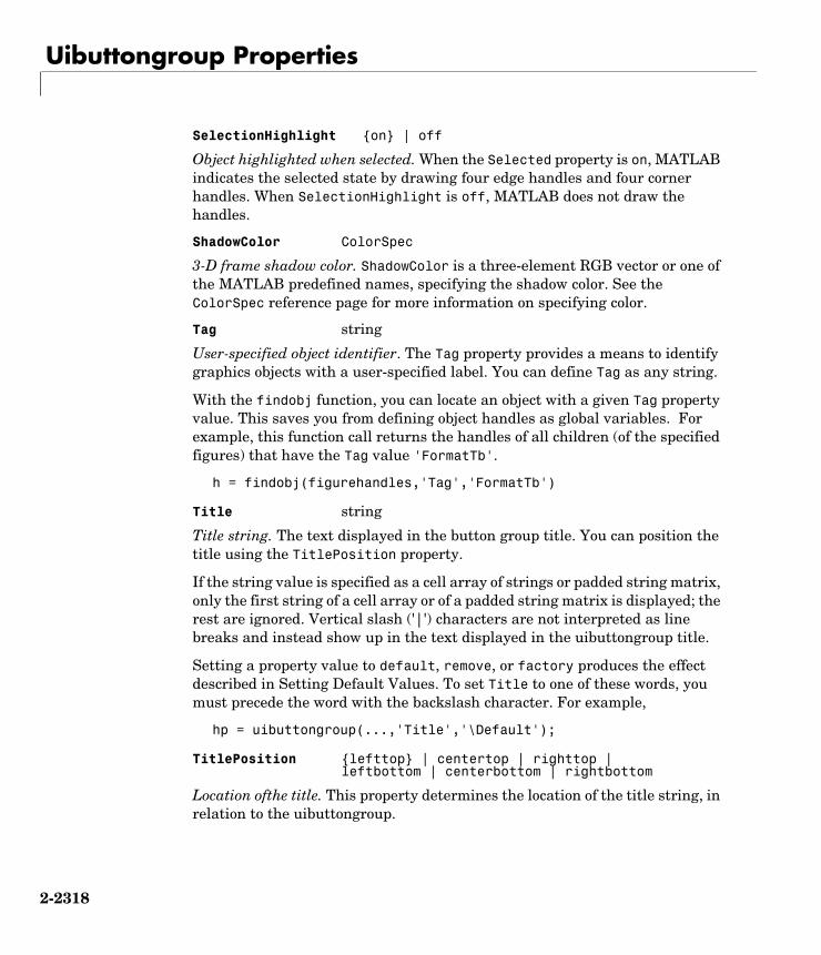
Uibuttongroup Properties
2-2318
SelectionHighlight on | off
Object highlighted when selected. When the Selected property is on, MATLAB indicates the selected state by drawing four edge handles and four corner handles. When SelectionHighlight is off, MATLAB does not draw the handles.
ShadowColor ColorSpec
3-D frame shadow color. ShadowColor is a three-element RGB vector or one of the MATLAB predefined names, specifying the shadow color. See the ColorSpec reference page for more information on specifying color.
Tag string
User-specified object identifier. The Tag property provides a means to identify graphics objects with a user-specified label. You can define Tag as any string.
With the findobj function, you can locate an object with a given Tag property value. This saves you from defining object handles as global variables. For example, this function call returns the handles of all children (of the specified figures) that have the Tag value 'FormatTb'.
h = findobj(figurehandles,'Tag','FormatTb')
Title string
Title string. The text displayed in the button group title. You can position the title using the TitlePosition property.
If the string value is specified as a cell array of strings or padded string matrix, only the first string of a cell array or of a padded string matrix is displayed; the rest are ignored. Vertical slash ('|') characters are not interpreted as line breaks and instead show up in the text displayed in the uibuttongroup title.
Setting a property value to default, remove, or factory produces the effect described in Setting Default Values. To set Title to one of these words, you must precede the word with the backslash character. For example,
hp = uibuttongroup(...,'Title','\Default');
TitlePosition lefttop | centertop | righttop |leftbottom | centerbottom | rightbottom
Location ofthe title. This property determines the location of the title string, in relation to the uibuttongroup.

Uibuttongroup Properties
2-2319
UIContextMenu handle
Associate a context menu with a uibuttongroup. Assign this property the handle of a Uicontextmenu object. MATLAB displays the context menu whenever you right-click the uibuttongroup. Use the uicontextmenu function to create the context menu.
Units inches | centimeters | normalized |points | pixels | characters
Units of measurement. MATLAB uses these units to interpret the Position property. All units are measured from the lower-left corner of the figure window.
• Normalized units map the lower-left corner of the figure window to (0,0) and the upper-right corner to (1.0,1.0).
• pixels, inches, centimeters, and points are absolute units (1 point = 1/72 inch).
• Character units are characters using the default system font; the width of one character is the width of the letter x, the height of one character is the distance between the baselines of two lines of text.
If you change the value of Units, it is good practice to return it to its default value after completing your computation so as not to affect other functions that assume Units is set to the default value.
UserData matrix
User-specified data. Any data you want to associate with the uibuttongroup object. MATLAB does not use this data, but you can access it using set and get.
Visible on | off
Uibuttongroup visibility. By default, a uibuttongroup object is visible. When set to off, the uibuttongroup is not visible, but still exists and you can query and set its properties.
Note The value of a uibuttongroup’s Visible property also controls the Visible property of child axes, uipanels, and uibuttongroups. This property does not affect the Visible property of child uicontrols.

uicontextmenu
2-2320
2uicontextmenuPurpose Create a context menu
Syntax handle = uicontextmenu('PropertyName',PropertyValue,...);
Description uicontextmenu creates a context menu, which is a menu that appears when the user right-clicks on a graphics object.
You create context menu items using the uimenu function. Menu items appear in the order the uimenu statements appear. You associate a context menu with an object using the UIContextMenu property for the object and specifying the context menu’s handle as the property value.
Properties This table lists all properties useful to uibuttongroup objects, grouping them by function. Each property name acts as a link to a description of the property. Curly braces denote the default value, if any.
This table lists the properties that are useful to uicontextmenu objects, grouping them by function. Each property name acts as a link to a description of the property.
Property Name Property Description Property Value
Controlling Style and Appearance
Visible Uicontextmenu visibility Value: on, offDefault: off
Position Location of uicontextmenu when Visible is set to on
Value: two-element vectorDefault: [0 0]
General Information About the Object
Children The uimenus defined for the uicontextmenu
Value: matrix
Parent Uicontextmenu object’s parent Value: scalar figure handle
Tag User-specified object identifier Value: string
Type Class of graphics object Value: string (read-only)Default: uicontrol

uicontextmenu
2-2321
Example These statements define a context menu associated with a line. When the user extend-clicks anywhere on the line, the menu appears. Menu items enable the user to change the line style.
% Define the context menucmenu = uicontextmenu;% Define the line and associate it with the context menuhline = plot(1:10, 'UIContextMenu', cmenu);% Define callbacks for context menu itemscb1 = ['set(hline, ''LineStyle'', ''--'')'];cb2 = ['set(hline, ''LineStyle'', '':'')'];cb3 = ['set(hline, ''LineStyle'', ''-'')'];% Define the context menu itemsitem1 = uimenu(cmenu, 'Label', 'dashed', 'Callback', cb1);item2 = uimenu(cmenu, 'Label', 'dotted', 'Callback', cb2);item3 = uimenu(cmenu, 'Label', 'solid', 'Callback', cb3);
UserData User-specified data Value: matrix
Controlling Callback Routine Execution
BusyAction Callback routine interruption Value: cancel, queueDefault: queue
Callback Control action Value: string
CreateFcn Callback routine executed during object creation
Value: string
DeleteFcn Callback routine executed during object deletion
Value: string
Interruptible Callback routine interruption mode Value: on, offDefault: on
Controlling Access to Objects
HandleVisibility Whether handle is accessible from command line and GUIs
Value: on, callback, offDefault: on
Property Name Property Description Property Value

uicontextmenu
2-2322
When the user extend-clicks on the line, the context menu appears, as shown in this figure:
See Also uibuttongroup, uicontrol, uimenu, uipanel

Uicontextmenu Properties
2-2323
2Uicontextmenu PropertiesModifying Properties
You can set and query graphics object properties in two ways:
• The Property Inspector is an interactive tool that enables you to see and change object property values. The Property inspector is available from GUIDE, or use the inspect function at the command line.
• The set and get functions enable you to set and query the values of properties.
For more information about changing the default value of a property see Setting Default Property Values. For an example, see the CreateFcn property.
UicontextmenuProperties
This section lists all properties useful to uicontextmenu objects along with valid values and descriptions of their use. Curly braces enclose default values.
Property Purpose
BusyAction Callback routine interruption
Callback Control action
Children The uimenus defined for the uicontextmenu
CreateFcn Callback routine executed during object creation
DeleteFcn Callback routine executed during object deletion
HandleVisibility Whether handle is accessible from command line and GUIs
Interruptible Callback routine interruption mode
Parent Uicontextmenu object’s parent
Position Location of uicontextmenu when Visible is set to on
Tag User-specified object identifier
Type Class of graphics object
UserData User-specified data
Visible Uicontextmenu visibility

Uicontextmenu Properties
2-2324
BusyAction cancel | queue
Callback routine interruption. If a callback is executing and the user triggers an event (such as a mouse click) on an object for which a callback is defined, the callback associated with the new event uses the value of BusyAction to decide whether or not to attempt to interrupt the executing callback.
• If the value is cancel, the event is discarded and the second callback does not execute.
• If the value is queue, and the Interruptible property of the first callback is on, the second callback is added to the event queue and executes in its turn after the first callback finishes execution.
Note If the interrupting callback is a DeleteFcn or CreateFcn callback or a figure’s CloseRequest or ResizeFcn callback, it interrupts an executing callback regardless of the value of that object’s Interruptible property. See the Interruptible property for information about controlling a callback’s interruptibility.
ButtonDownFcn string
This property has no effect on uicontextmenu objects.
Callback string
Control action. A routine that executes whenever you right-click an object for which a context menu is defined. The routine executes immediately before the context menu is posted. Define this routine as a string that is a valid MATLAB expression or the name of an M-file. The expression executes in the MATLAB workspace.
Children matrix
The uimenus defined for the uicontextmenu.
Clipping on | off
This property has no effect on uicontextmenu objects.
CreateFcn string
Callback routine executed during object creation. The specified function executes when MATLAB creates a uicontextmenu object. MATLAB sets all

Uicontextmenu Properties
2-2325
property values for the uicontextmenu before executing the CreateFcn callback so these values are available to the callback. Within the function, use gcbo to get the handle of the uicontextmenu being created.
Setting this property on an existing uicontextmenu object has no effect.
You can define a default CreateFcn callback for all new uicontextmenus. This default applies unless you override it by specifying a different CreateFcn callback when you call uicontextmenu. For example, the code
set(0,'DefaultUicontextmenuCreateFcn','set(gcbo,... ''Visible'',''on'')')
creates a default CreateFcn callback that runs whenever you create a new context menu. It sets the default Visible property of a context menu.
To override this default and create a context menu whose Visible property is set to a different value, call uicontextmenu with code similar to
hpt = uicontextmenu(...,'CreateFcn','set(gcbo,...''Visible'',''off'')')
Note To override a default CreateFcn callback you must provide a new callback and not just provide different values for the specified properties. This is because the CreateFcn callback runs after the property values are set, and can override property values you have set explicitly in the uicontextmenu call. In the example above, if instead of redefining the CreateFcn property for this uicontextmenu, you had explicitly set Visible to off, the default CreateFcn callback would have set Visible back to the default, i.e., on.
See Function Handle Callbacks for information on how to use function handles to define a callback function.
DeleteFcn string
Delete uicontextmenu callback routine. A callback routine that executes when you delete the uicontextmenu object (e.g., when you issue a delete command or clear the figure containing the uicontextmenu). MATLAB executes the routine before destroying the object’s properties so these values are available to the callback routine.

Uicontextmenu Properties
2-2326
The handle of the object whose DeleteFcn is being executed is accessible only through the root CallbackObject property, which you can query using gcbo.
See Function Handle Callbacks for information on how to use function handles to define a callback function.
HandleVisibility on | callback | off
Control access to object’s handle. This property determines when an object’s handle is visible in its parent’s list of children. When a handle is not visible in its parent’s list of children, it is not returned by functions that obtain handles by searching the object hierarchy or querying handle properties. This includes get, findobj, gca, gcf, gco, newplot, cla, clf, and close. Neither is the handle visible in the parent figure’s CurrentObject property. Handles that are hidden are still valid. If you know an object’s handle, you can set and get its properties, and pass it to any function that operates on handles.
• Handles are always visible when HandleVisibility is on.
• Setting HandleVisibility to callback causes handles to be visible from within callback routines or functions invoked by callback routines, but not from within functions invoked from the command line. This provides a means to protect GUIs from command-line users, while allowing callback routines to have complete access to object handles.
• Setting HandleVisibility to off makes handles invisible at all times. This may be necessary when a callback routine invokes a function that might potentially damage the GUI (such as evaluating a user-typed string), and so temporarily hides its own handles during the execution of that function.
You can set the root ShowHiddenHandles property to on to make all handles visible, regardless of their HandleVisibility settings. This does not affect the values of the HandleVisibility properties.
HitTest on | off
This property has no effect on uicontextmenu objects.
Interruptible on | off
Callback routine interruption mode. If a callback is executing and the user triggers an event (such as a mouse click) on an object for which a callback is defined, that callback attempts to interrupt the first callback. MATLAB processes the callbacks according to these factors:
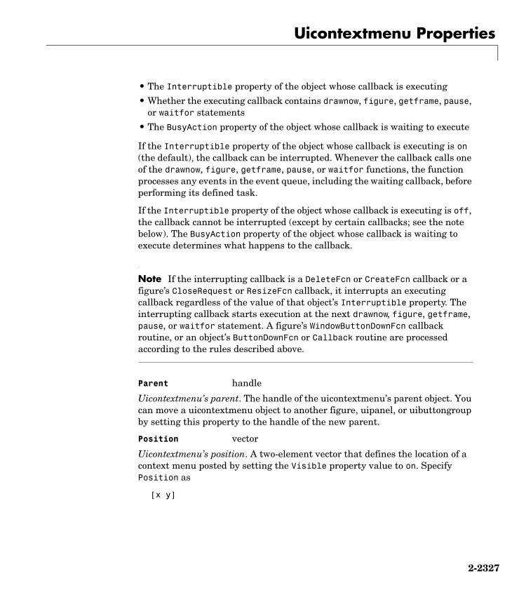
Uicontextmenu Properties
2-2327
• The Interruptible property of the object whose callback is executing
• Whether the executing callback contains drawnow, figure, getframe, pause, or waitfor statements
• The BusyAction property of the object whose callback is waiting to execute
If the Interruptible property of the object whose callback is executing is on (the default), the callback can be interrupted. Whenever the callback calls one of the drawnow, figure, getframe, pause, or waitfor functions, the function processes any events in the event queue, including the waiting callback, before performing its defined task.
If the Interruptible property of the object whose callback is executing is off, the callback cannot be interrupted (except by certain callbacks; see the note below). The BusyAction property of the object whose callback is waiting to execute determines what happens to the callback.
Note If the interrupting callback is a DeleteFcn or CreateFcn callback or a figure’s CloseRequest or ResizeFcn callback, it interrupts an executing callback regardless of the value of that object’s Interruptible property. The interrupting callback starts execution at the next drawnow, figure, getframe, pause, or waitfor statement. A figure’s WindowButtonDownFcn callback routine, or an object’s ButtonDownFcn or Callback routine are processed according to the rules described above.
Parent handle
Uicontextmenu’s parent. The handle of the uicontextmenu’s parent object. You can move a uicontextmenu object to another figure, uipanel, or uibuttongroup by setting this property to the handle of the new parent.
Position vector
Uicontextmenu’s position. A two-element vector that defines the location of a context menu posted by setting the Visible property value to on. Specify Position as
[x y]

Uicontextmenu Properties
2-2328
where vector elements represent the horizontal and vertical distances in pixels from the bottom left corner of the figure window, panel, or button group to the top left corner of the context menu.
Selected on | off
This property has no effect on uicontextmenu objects.
SelectionHighlight on | off
This property has no effect on uicontextmenu objects.
Tag string
User-specified object label. The Tag property provides a means to identify graphics objects with a user-specified label. This is particularly useful when constructing interactive graphics programs that would otherwise need to define object handles as global variables or pass them as arguments between callback routines. You can define Tag as any string.
Type string
Class of graphics object. For uicontextmenu objects, Type is always the string 'uicontextmenu'.
UIContextMenu handle
This property has no effect on uicontextmenus.
UserData matrix
User-specified data. Any data you want to associate with the uicontextmenu object. MATLAB does not use this data, but you can access it using set and get.
Visible on | off
Uicontextmenu visibility. The Visible property can be used in two ways:
• Its value indicates whether the context menu is currently posted. While the context menu is posted, the property value is on; when the context menu is not posted, its value is off.
• Its value can be set to on to force the posting of the context menu. Similarly, setting the value to off forces the context menu to be removed. When used in this way, the Position property determines the location of the posted context menu.
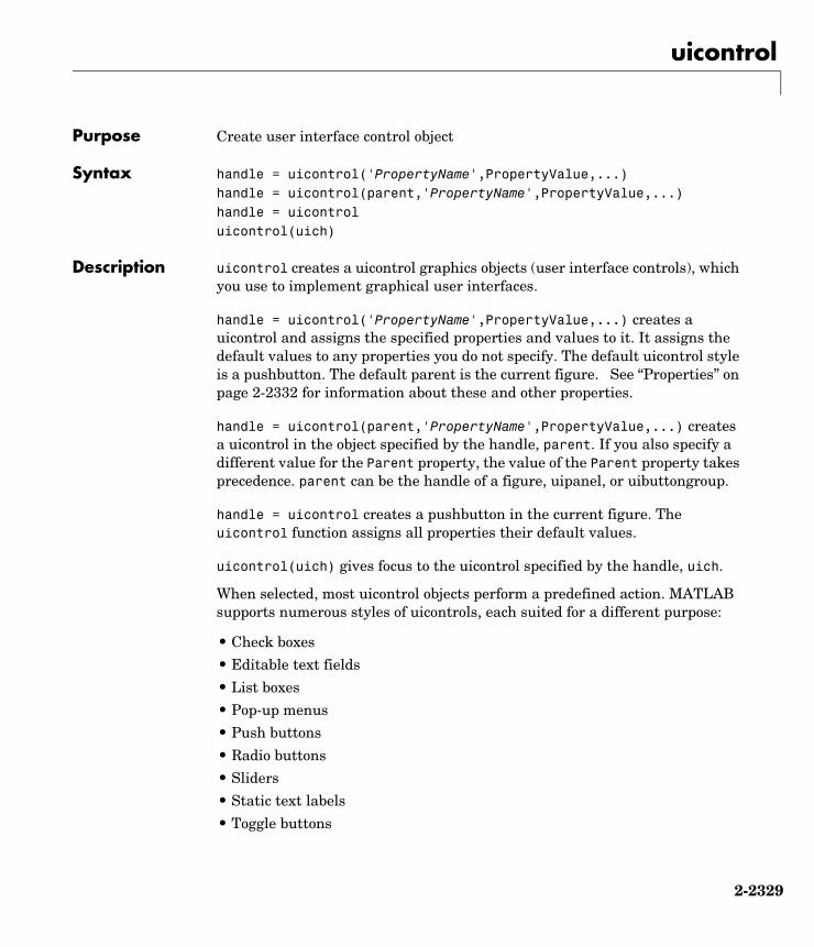
uicontrol
2-2329
2uicontrolPurpose Create user interface control object
Syntax handle = uicontrol('PropertyName',PropertyValue,...)handle = uicontrol(parent,'PropertyName',PropertyValue,...)handle = uicontroluicontrol(uich)
Description uicontrol creates a uicontrol graphics objects (user interface controls), which you use to implement graphical user interfaces.
handle = uicontrol('PropertyName',PropertyValue,...) creates a uicontrol and assigns the specified properties and values to it. It assigns the default values to any properties you do not specify. The default uicontrol style is a pushbutton. The default parent is the current figure. See “Properties” on page 2-2332 for information about these and other properties.
handle = uicontrol(parent,'PropertyName',PropertyValue,...) creates a uicontrol in the object specified by the handle, parent. If you also specify a different value for the Parent property, the value of the Parent property takes precedence. parent can be the handle of a figure, uipanel, or uibuttongroup.
handle = uicontrol creates a pushbutton in the current figure. The uicontrol function assigns all properties their default values.
uicontrol(uich) gives focus to the uicontrol specified by the handle, uich.
When selected, most uicontrol objects perform a predefined action. MATLAB supports numerous styles of uicontrols, each suited for a different purpose:
• Check boxes
• Editable text fields
• List boxes
• Pop-up menus
• Push buttons
• Radio buttons
• Sliders
• Static text labels
• Toggle buttons

uicontrol
2-2330
For information on using these uicontrols within GUIDE, the MATLAB GUI development environment, see
• Setting Component Properties — the Property Inspector
• Programming Callbacks for GUI Components
Specifying the Uicontrol Style To create a specific type of uicontrol, set the Style property as one of the following strings:
• 'checkbox'– Check boxes generate an action when selected. These devices are useful when providing the user with a number of independent choices. To activate a check box, click the mouse button on the object. The state of the device is indicated on the display.
• 'edit' – Editable text fields enable users to enter or modify text values. Use editable text when you want text as input. If Max-Min>1, then multiple lines are allowed. For multi-line edit boxes, a vertical scrollbar enables scrolling, as do the arrow keys.
• 'listbox' – List boxes display a list of items (defined using the String property) and enable users to select one or more items. The Min and Max properties control the selection mode:
If Max-Min>1, then multiple selection is allowed.
If Max-Min<=1, then only single selection is allowed.
The Value property indicates selected entries and contains the indices into the list of strings; a vector value indicates multiple selections. MATLAB evaluates the list box’s callback routine after any mouse button up event that changes the Value property. Therefore, you may need to add a “Done” button to delay action caused by multiple clicks on list items. List boxes differentiate between single and double clicks and set the figure SelectionType property to normal or open accordingly before evaluating the list box’s Callback property.
• 'popupmenu' – Pop-up menus open to display a list of choices (defined using the String property) when pressed. When not open, a pop-up menu indicates the current choice. Pop-up menus are useful when you want to provide users with a number of mutually exclusive choices, but do not want to take up the

uicontrol
2-2331
amount of space that a series of radio buttons requires. You must specify a value for the String property.
• 'pushbutton' – Push buttons generate an action when pressed. To activate a push button, click the mouse button on the push button.
• 'radiobutton' – Radio buttons are similar to check boxes, but are intended to be mutually exclusive within a group of related radio buttons (i.e., only one is in a pressed state at any given time). To activate a radio button, click the mouse button on the object. The state of the device is indicated on the display. Note that your code can implement the mutually exclusive behavior of radio buttons.
• 'slider' – Sliders accept numeric input within a specific range by enabling the user to move a sliding bar. Users move the bar by pressing the mouse button and dragging the pointer over the bar, or by clicking in the trough or on an arrow. The location of the bar indicates a numeric value, which is selected by releasing the mouse button. You can set the minimum, maximum, and current values of the slider.
• 'text' – Static text boxes display lines of text. Static text is typically used to label other controls, provide directions to the user, or indicate values associated with a slider. Users cannot change static text interactively and there is no way to invoke the callback routine associated with it.
• 'toggle' – Toggle buttons are controls that execute callbacks when clicked on and indicate their state, either on or off. Toggle buttons are useful for building toolbars.
Remarks The uicontrol function accepts property name/property value pairs, structures, and cell arrays as input arguments and optionally returns the handle of the created object. You can also set and query property values after creating the object using the set and get functions.
A uicontrol object is a child of a figure, uipanel, or uibuttongroup and therefore does not require an axes to exist when placed in a figure window, uipanel, or uibuttongroup.

uicontrol
2-2332
Properties This table lists all properties useful for uicontrol objects, grouping them by function. Each property name acts as a link to a description of the property.
Property Name Property Description Property Value
Controlling Style and Appearance
BackgroundColor Object background color Value: ColorSpecDefault: system dependent
CData Truecolor image displayed on the control
Value: matrix
ForegroundColor Color of text Value: ColorSpecDefault: [0 0 0]
SelectionHighlight Object highlighted when selected Value: on, offDefault: on
String Uicontrol label, also list box and pop-up menu items
Value: string
Visible Uicontrol visibility Value: on, offDefault: on
General Information About the Object
Children Uicontrol objects have no children
Enable Enable or disable the uicontrol Value: on, inactive, offDefault: on
Parent Uicontrol object’s parent Value: figure, uipanel, or uibuttongroup handle
Selected Whether object is selected Value: on, offDefault: off
SliderStep Slider step size Value: two-element vectorDefault: [0.01 0.1]

uicontrol
2-2333
Style Type of uicontrol object Value: pushbutton, togglebutton, radiobutton, checkbox, edit, text, slider, listbox, popupmenuDefault: pushbutton
Tag User-specified object identifier Value: string
TooltipString Content of object’s tooltip Value: string
Type Class of graphics object Value: string (read-only)Default: uicontrol
UserData User-specified data Value: matrix
Controlling the Object Position
Position Size and location of uicontrol object Value: position rectangleDefault: [20 20 60 20]
Units Units to interpret position vector Value: pixels, normalized, inches, centimeters, points, charactersDefault: pixels
Controlling Fonts and Labels
FontAngle Character slant Value: normal, italic, obliqueDefault: normal
FontName Font family Value: stringDefault: system dependent
FontSize Font size Value: size in FontUnitsDefault: system dependent
Property Name Property Description Property Value

uicontrol
2-2334
FontUnits Font size units Value: points, normalized, inches, centimeters, pixelsDefault: points
FontWeight Weight of text characters Value: light, normal, demi, boldDefault: normal
HorizontalAlignment Alignment of label string Value: left, center, rightDefault: depends on uicontrol object
String Uicontrol object label, also list box and pop-up menu items
Value: string
Controlling Callback Routine Execution
BusyAction Callback routine interruption Value: cancel, queueDefault: queue
ButtonDownFcn Button-press callback routine Value: string or function handle
Callback Control action Value: string or function handle
CreateFcn Callback routine executed during object creation
Value: string or function handle
DeleteFcn Callback routine executed during object deletion
Value: string or function handle
Interruptible Callback routine interruption mode Value: on, offDefault: on
KeyPressFcn Key press callback routine Value: string or function handle
UIContextMenu Uicontextmenu object associated with the uicontrol
Value: handle
Property Name Property Description Property Value

uicontrol
2-2335
Examples Example 1. The following statement creates a push button that clears the current axes when pressed.
h = uicontrol('Style', 'pushbutton', 'String', 'Clear',...'Position', [20 150 100 70], 'Callback', 'cla');
This statement gives focus to the pushbutton.
uicontrol(h)
Example 2. You can create a uicontrol object that changes figure colormaps by specifying a pop-up menu and supplying an M-file name as the object’s Callback:
hpop = uicontrol('Style', 'popup',...'String', 'hsv|hot|cool|gray',...'Position', [20 320 100 50],...'Callback', 'setmap');
Information About the Current State
ListboxTop Index of top-most string displayed in list box
Value: scalarDefault: [1]
Max Maximum value (depends on uicontrol object)
Value: scalarDefault: object dependent
Min Minimum value (depends on uicontrol object)
Value: scalarDefault: object dependent
Value Current value of uicontrol object Value: scalar or vectorDefault: object dependent
Controlling Access to Objects
HandleVisibility Whether handle is accessible from command line and GUIs
Value: on, callback, offDefault: on
HitTest Whether selectable by mouse click Value: on, offDefault: on
Property Name Property Description Property Value

uicontrol
2-2336
The above call to uicontrol defines four individual choices in the menu: hsv, hot, cool, and gray. You specify these choices with the String property, separating the choices with the “|” character.
The Callback, in this case setmap, is the name of an M-file that defines a more complicated set of instructions than a single MATLAB command. setmap contains these statements:
val = get(hpop,'Value');if val == 1
colormap(hsv)elseif val == 2
colormap(hot)elseif val == 3
colormap(cool)elseif val == 4
colormap(gray)end
The Value property contains a number that indicates the selected choice. The choices are numbered sequentially from one to four. The setmap M-file can get and then test the contents of the Value property to determine what action to take.
See Also textwrap, uibuttongroup, uimenu, uipanel

Uicontrol Properties
2-2337
2Uicontrol PropertiesModifying Properties
You can set and query graphics object properties in two ways:
• The Property Inspector is an interactive tool that enables you to see and change object property values. The Property inspector is available from GUIDE, or use the inspect function at the command line.
• The set and get commands enable you to set and query the values of properties
To change the default value of properties see Setting Default Property Values. You can also set default uicontrol properties on the root and figure levels:
set(0,'DefaultUicontrolProperty',PropertyValue...)set(gcf,'DefaultUicontrolProperty',PropertyValue...)
where Property is the name of the uicontrol property whose default value you want to set and PropertyValue is the value you are specifying as the default. Use set and get to access uicontrol properties.
For information on using these uicontrols within GUIDE, the MATLAB GUI development environment, see
• Setting Component Properties — the Property Inspector
• Programming Callbacks for GUI Components
Uicontrol Properties
This section lists all properties useful to uicontrol objects along with valid values and descriptions of their use. Curly braces enclose default values.
Property Purpose
BackgroundColor Object background color
BusyAction Callback routine interruption
ButtonDownFcn Button-press callback routine
Callback Control action
CData Truecolor image displayed on the control
Children Uicontrol objects have no children

Uicontrol Properties
2-2338
CreateFcn Callback routine executed during object creation
DeleteFcn Callback routine executed during object deletion
Enable Enable or disable the uicontrol
FontAngle Character slant
FontName Font family
FontSize Font size
FontUnits Font size units
FontWeight Weight of text characters
ForegroundColor Color of text
HandleVisibility Whether handle is accessible from command line and GUIs
HitTest Whether selectable by mouse click
HorizontalAlignment Alignment of label string
Interruptible Callback routine interruption mode
KeyPressFcn Key press callback routine
ListboxTop Index of top-most string displayed in list box
Max Maximum value (depends on uicontrol object)
Min Minimum value (depends on uicontrol object)
Parent Uicontrol object’s parent
Position Size and location of uicontrol object
Selected Whether object is selected
SelectionHighlight Object highlighted when selected
Property Purpose

Uicontrol Properties
2-2339
BackgroundColor ColorSpec
Object background color. The color used to fill the uicontrol rectangle. Specify a color using a three-element RGB vector or one of the MATLAB predefined names. The default color is determined by system settings. See ColorSpec for more information on specifying color.
BusyAction cancel | queue
Callback routine interruption. If a callback is executing and the user triggers an event (such as a mouse click) on an object for which a callback is defined, the callback associated with the new event uses the value of BusyAction to decide whether or not to attempt to interrupt the executing callback.
• If the value is cancel, the event is discarded and the second callback does not execute.
SliderStep Slider step size
String Uicontrol label, also list box and pop-up menu items
String Uicontrol object label, also list box and pop-up menu items
Style Type of uicontrol object
Tag User-specified object identifier
TooltipString Content of object’s tooltip
Type Class of graphics object
UIContextMenu Uicontextmenu object associated with the uicontrol
Units Units to interpret position vector
UserData User-specified data
Value Current value of uicontrol object
Visible Uicontrol visibility
Property Purpose

Uicontrol Properties
2-2340
• If the value is queue, and the Interruptible property of the first callback is on, the second callback is added to the event queue and executes in its turn after the first callback finishes execution.
Note If the interrupting callback is a DeleteFcn or CreateFcn callback or a figure’s CloseRequest or ResizeFcn callback, it interrupts an executing callback regardless of the value of that object’s Interruptible property. See the Interruptible property for information about controlling a callback’s interruptibility.
ButtonDownFcn string or function handle (GUIDE sets this property)
Button-press callback routine. A callback routine that executes when you press a mouse button while the pointer is in a 5-pixel wide border around the uicontrol. When the uicontrol’s Enable property is set to inactive or off, the ButtonDownFcn executes when you click the mouse in the 5-pixel border or on the control itself. This is useful for implementing actions to interactively modify control object properties, such as size and position, when they are clicked on (using selectmoveresize, for example).
Define this routine as a string that is a valid MATLAB expression or the name of an M-file. The expression executes in the MATLAB workspace.
To add a ButtonDownFcn callback in GUIDE, select View Callbacks from the Layout Editor View menu, then select ButtonDownFcn. GUIDE sets this property to the appropriate string and adds the callback to the M-file the next time you save the GUI. Alternatively, you can set this property to the string %automatic. The next time you save the GUI, GUIDE sets this property to the appropriate string and adds the callback to the M-file.
Use the Callback property to specify the callback routine that executes when you activate the enabled uicontrol (e.g., click on a push button).
Callback string (GUIDE sets this property)
Control action. A routine that executes whenever you activate the uicontrol object (e.g., when you click on a push button or move a slider). Define this routine as a string that is a valid MATLAB expression or the name of an M-file. The expression executes in the MATLAB workspace.

Uicontrol Properties
2-2341
To execute the callback routine for an edit text control, type in the desired text and then do one of the following:
• Click another component, the menu bar, or the background of the GUI.
• For a single line editable text box, press Enter, or
• For a multiline editable text box, press Ctl+Enter.
Callback routines defined for static text do not execute because no action is associated with these objects.
CData matrix
Truecolor image displayed on control. A three-dimensional matrix of RGB values that defines a truecolor image displayed on either a push button or toggle button. Each value must be between 0.0 and 1.0.
Children matrix
The empty matrix; uicontrol objects have no children.
Clipping on | off
This property has no effect on uicontrols.
CreateFcn string
Callback routine executed during object creation. The specified function executes when MATLAB creates a uicontrol object. MATLAB sets all property values for the uiconrtol before executing the CreateFcn callback so these values are available to the callback. Within the function, use gcbo to get the handle of the uicontrol being created.
Setting this property on an existing uicontrol object has no effect.
You can define a default CreateFcn callback for all new uicontrols. This default applies unless you override it by specifying a different CreateFcn callback when you call uicontrol. For example, the code
set(0,'DefaultUicontrolCreateFcn','set(gcbo,... ''BackgroundColor'',''white'')')
creates a default CreateFcn callback that runs whenever you create a new uicontrol. It sets the default background color of all new uicontrols.
To override this default and create a uicontrol whose BackgroundColor is set to a different value, call uicontrol with code similar to

Uicontrol Properties
2-2342
hpt = uicontrol(...,'CreateFcn','set(gcbo,...''BackgroundColor'',''blue'')')
Note To override a default CreateFcn callback you must provide a new callback and not just provide different values for the specified properties. This is because the CreateFcn callback runs after the property values are set, and can override property values you have set explicitly in the uicontrol call. In the example above, if instead of redefining the CreateFcn property for this uicontrol, you had explicitly set BackgroundColor to blue, the default CreateFcn callback would have set BackgroundColor back to the default, i.e., white.
See Function Handle Callbacks for information on how to use function handles to define a callback function.
DeleteFcn string
Delete uicontrol callback routine. A callback routine that executes when you delete the uicontrol object (e.g., when you issue a delete command or clear the figure containing the uicontrol). MATLAB executes the routine before destroying the object’s properties so these values are available to the callback routine.
The handle of the object whose DeleteFcn is being executed is accessible only through the root CallbackObject property, which you can query using gcbo.
See Function Handle Callbacks for information on how to use function handles to define a callback function.
Enable on | inactive | off
Enable or disable the uicontrol. This property controls how uicontrols respond to mouse button clicks, including which callback routines execute.
• on – The uicontrol is operational (the default).
• inactive – The uicontrol is not operational, but looks the same as when Enable is on.
• off – The uicontrol is not operational and its image (set by the Cdata property) is grayed out.

Uicontrol Properties
2-2343
When you left-click on a uicontrol whose Enable property is on, MATLAB performs these actions in this order:
1 Sets the figure’s SelectionType property.
2 Executes the uicontrol’s ClickedCallback routine.
3 Does not set the figure’s CurrentPoint property and does not execute either the control’s ButtonDownFcn or the figure’s WindowButtonDownFcn callback.
When you left-click on a uitoggletool whose Enable property is off, or when you right-click a uicontrol whose Enable property has any value, MATLAB performs these actions in this order:
1 Sets the figure’s SelectionType property.
2 Sets the figure’s CurrentPoint property.
3 Executes the figure’s WindowButtonDownFcn callback.
Extent position rectangle (read only)
Size of uicontrol character string. A four-element vector that defines the size and position of the character string used to label the uicontrol. It has the form:
[0,0,width,height]
The first two elements are always zero. width and height are the dimensions of the rectangle. All measurements are in units specified by the Units property.
Since the Extent property is defined in the same units as the uicontrol itself, you can use this property to determine proper sizing for the uicontrol with regard to its label. Do this by
• Defining the String property and selecting the font using the relevant properties.
• Getting the value of the Extent property.
• Defining the width and height of the Position property to be somewhat larger than the width and height of the Extent.
For multiline strings, the Extent rectangle encompasses all the lines of text. For single line strings, the Extent is returned as a single line, even if the string wraps when displayed on the control.

Uicontrol Properties
2-2344
FontAngle normal | italic | oblique
Character slant. MATLAB uses this property to select a font from those available on your particular system. Setting this property to italic or oblique selects a slanted version of the font, when it is available on your system.
FontName string
Font family. The name of the font in which to display the String. To display and print properly, this must be a font that your system supports. The default font is system dependent.
To use a fixed-width font that looks good in any locale (and displays properly in Japan, where multibyte character sets are used), set FontName to the string FixedWidth (this string value is case sensitive):
set(uicontrol_handle, 'FontName', 'FixedWidth')
This parameter value eliminates the need to hard code the name of a fixed-width font, which may not display text properly on systems that do not use ASCII character encoding (such as in Japan). A properly written MATLAB application that needs to use a fixed-width font should set FontName to FixedWidth and rely on the root FixedWidthFontName property to be set correctly in the end user’s environment.
End users can adapt a MATLAB application to different locales or personal environments by setting the root FixedWidthFontName property to the appropriate value for that locale from startup.m. Setting the root FixedWidthFontName property causes an immediate update of the display to use the new font.
FontSize size in FontUnits
Font size. A number specifying the size of the font in which to display the String, in units determined by the FontUnits property. The default point size is system dependent.
FontUnits points | normalized | inches |centimeters | pixels
Font size units. This property determines the units used by the FontSize property. Normalized units interpret FontSize as a fraction of the height of the uicontrol. When you resize the uicontrol, MATLAB modifies the screen FontSize accordingly. pixels, inches, centimeters, and points are absolute units (1 point = 1/72 inch).

Uicontrol Properties
2-2345
FontWeight light | normal | demi | bold
Weight of text characters. MATLAB uses this property to select a font from those available on your particular system. Setting this property to bold causes MATLAB to use a bold version of the font, when it is available on your system.
ForegroundColor ColorSpec
Color of text. This property determines the color of the text defined for the String property (the uicontrol label). Specify a color using a three-element RGB vector or one of MATLAB ’s predefined names. The default text color is black. See ColorSpec for more information on specifying color.
HandleVisibility on | callback | off
Control access to object’s handle. This property determines when an object’s handle is visible in its parent’s list of children. When a handle is not visible in its parent’s list of children, it is not returned by functions that obtain handles by searching the object hierarchy or querying handle properties. This includes get, findobj, gca, gcf, gco, newplot, cla, clf, and close. Neither is the handle visible in the parent figure’s CurrentObject property. Handles that are hidden are still valid. If you know an object’s handle, you can set and get its properties, and pass it to any function that operates on handles.
• Handles are always visible when HandleVisibility is on.
• Setting HandleVisibility to callback causes handles to be visible from within callback routines or functions invoked by callback routines, but not from within functions invoked from the command line. This provides a means to protect GUIs from command-line users, while allowing callback routines to have complete access to object handles.
• Setting HandleVisibility to off makes handles invisible at all times. This may be necessary when a callback routine invokes a function that might potentially damage the GUI (such as evaluating a user-typed string), and so temporarily hides its own handles during the execution of that function.
You can set the root ShowHiddenHandles property to on to make all handles visible, regardless of their HandleVisibility settings. This does not affect the values of the HandleVisibility properties.

Uicontrol Properties
2-2346
Note Radio buttons and toggle buttons that are managed by a uibuttongroup should not be accessed outside the button group. Set the HandleVisibility of such radio buttons and toggle buttons to off to prevent inadvertent access.
HitTest on | off
Selectable by mouse click. This property has no effect on uicontrol objects.
HorizontalAlignment left | center | right
Horizontal alignment of label string. This property determines the justification of the text defined for the String property (the uicontrol label):
• left — Text is left justified with respect to the uicontrol.
• center — Text is centered with respect to the uicontrol.
• right — Text is right justified with respect to the uicontrol.
On Microsoft Windows systems, this property affects only edit and text uicontrols.
Interruptible on | off
Callback routine interruption mode. If a callback is executing and the user triggers an event (such as a mouse click) on an object for which a callback is defined, that callback attempts to interrupt the first callback. MATLAB processes the callbacks according to these factors:
• The Interruptible property of the object whose callback is executing
• Whether the executing callback contains drawnow, figure, getframe, pause, or waitfor statements
• The BusyAction property of the object whose callback is waiting to execute
If the Interruptible property of the object whose callback is executing is on (the default), the callback can be interrupted. Whenever the callback calls one of the drawnow, figure, getframe, pause, or waitfor functions, the function processes any events in the event queue, including the waiting callback, before performing its defined task.
If the Interruptible property of the object whose callback is executing is off, the callback cannot be interrupted (except by certain callbacks; see the note

Uicontrol Properties
2-2347
below). The BusyAction property of the object whose callback is waiting to execute determines what happens to the callback.
Note If the interrupting callback is a DeleteFcn or CreateFcn callback or a figure’s CloseRequest or ResizeFcn callback, it interrupts an executing callback regardless of the value of that object’s Interruptible property. The interrupting callback starts execution at the next drawnow, figure, getframe, pause, or waitfor statement. A figure’s WindowButtonDownFcn callback routine, or an object’s ButtonDownFcn or Callback routine are processed according to the rules described above.
KeyPressFcn string or function handle
Key press callback function. A callback routine invoked by a key press when the callback’s uicontrol object has focus. Focus is denoted by a border or a dotted border, respectively, in UNIX and Microsoft Windows. If no uicontrol has focus, the figure’s key press callback function, if any, is invoked. KeyPressFcn can be a function handle, the name of an M-file, or any legal MATLAB expression.
If the specified value is the name of an M-file, the callback routine can query the figure's CurrentCharacter property to determine what particular key was pressed and thereby limit the callback execution to specific keys.

Uicontrol Properties
2-2348
If the specified value is a function handle, the callback routine can retrieve information about the key that was pressed from its event data structure argument.
See Function Handle Callbacks for information on how to use function handles to define the callback function.
ListboxTop scalar
Index of top-most string displayed in list box. This property applies only to the listbox style of uicontrol. It specifies which string appears in the top-most position in a list box that is not large enough to display all list entries. ListboxTop is an index into the array of strings defined by the String property and must have a value between 1 and the number of strings. Noninteger values are fixed to the next lowest integer.
Max scalar
Maximum value. This property specifies the largest value allowed for the Value property. Different styles of uicontrols interpret Max differently:
• Check boxes – Max is the setting of the Value property while the check box is selected.
Event Data Structure Field
Description Examples:
a = Shift Shift/a
Character Character interpretation of the key that was pressed.
'a' '=' '' 'A'
Modifier Current modifier, such as 'control', or an empty cell array if there is no modifier
1x0 cell
1x0 cell
'shift' 'shift'
Key Name of the key that was pressed.
'a' 'equal' 'shift' 'a'

Uicontrol Properties
2-2349
• Editable text – If Max − Min > 1, then editable text boxes accept multiline input. If Max − Min <= 1, then editable text boxes accept only single line input.
• List boxes – If Max − Min > 1, then list boxes allow multiple item selection. If Max − Min <= 1, then list boxes do not allow multiple item selection.
• Radio buttons – Max is the setting of the Value property when the radio button is selected.
• Sliders – Max is the maximum slider value and must be greater than the Min property. The default is 1.
• Toggle buttons – Max is the value of the Value property when the toggle button is selected. The default is 1.
• Pop-up menus, push buttons, and static text do not use the Max property.
Min scalar
Minimum value. This property specifies the smallest value allowed for the Value property. Different styles of uicontrols interpret Min differently:
• Check boxes – Min is the setting of the Value property while the check box is not selected.
• Editable text – If Max − Min > 1, then editable text boxes accept multiline input. If Max − Min <= 1, then editable text boxes accept only single line input.
• List boxes – If Max − Min > 1, then list boxes allow multiple item selection. If Max − Min <= 1, then list boxes allow only single item selection.
• Radio buttons – Min is the setting of the Value property when the radio button is not selected.
• Sliders – Min is the minimum slider value and must be less than Max. The default is 0.
• Toggle buttons – Min is the value of the Value property when the toggle button is not selected. The default is 0.
• Pop-up menus, push buttons, and static text do not use the Min property.
Parent handle
Uicontrol parent. The handle of the uicontrol’s parent object. You can move a uicontrol object to another figure, uipanel, or uibuttongroup by setting this property to the handle of the new parent.

Uicontrol Properties
2-2350
Position position rectangle
Size and location of uicontrol. The rectangle defined by this property specifies the size and location of the control within the parent figure window, uipanel, or uibuttongroup. Specify Position as
[left bottom width height]
left and bottom are the distance from the lower-left corner of the parent object to the lower-left corner of the uicontrol object. width and height are the dimensions of the uicontrol rectangle. All measurements are in units specified by the Units property.
On Microsoft Windows systems, the height of pop-up menus is automatically determined by the size of the font. The value you specify for the height of the Position property has no effect.
The width and height values determine the orientation of sliders. If width is greater than height, then the slider is oriented horizontally, If height is greater than width, then the slider is oriented vertically.
Selected on | off (read only)
Is object selected. When this property is on, MATLAB displays selection handles if the SelectionHighlight property is also on. You can, for example, define the ButtonDownFcn to set this property, allowing users to select the object with the mouse.
SelectionHighlight on | off
Object highlight when selected. When the Selected property is on, MATLAB indicates the selected state by drawing four edge handles and four corner handles. When SelectionHighlight is off, MATLAB does not draw the handles.
SliderStep [min_step max_step]
Slider step size. This property controls the amount the slider Value changes when you click the mouse on the arrow button (min_step) or on the slider trough (max_step). Specify SliderStep as a two-element vector; each value must be in the range [0, 1]. The actual step size is a function of the specified SliderStep and the total slider range (Max − Min). The default, [0.01 0.10], provides a 1 percent change for clicks on the arrow button and a 10 percent change for clicks in the trough.

Uicontrol Properties
2-2351
For example, if you create the following slider,
uicontrol('Style','slider','Min',1,'Max',7,...'SliderStep',[0.1 0.6])
clicking on the arrow button moves the indicator by,
0.1*(7 1)ans =
0.6000
and clicking in the trough moves the indicator by,
0.6*(7 1)ans =
3.6000
Note that if the specified step size moves the slider to a value outside the range, the indicator moves only to the Max or Min value.
See also the Max, Min, and Value properties.
String string
Uicontrol label, list box items, pop-up menu choices. For check boxes, editable text, push buttons, radio buttons, static text, and toggle buttons, the text displayed on the object. For list boxes and pop-up menus, the set of entries or items displayed in the object.
For uicontrol objects that display only one line of text, if the string value is specified as a cell array of strings or padded string matrix, only the first string of a cell array or of a padded string matrix is displayed; the rest are ignored. Vertical slash ('|') characters are not interpreted as line breaks and instead show up in the text displayed in the uicontrol.
For multiple line editable text or static text controls, line breaks occur between each row of the string matrix, each cell of a cell array of strings, and after any \n characters embedded in the string. Vertical slash ('|') characters are not interpreted as line breaks, and instead show up in the text displayed in the uicontrol.
For multiple items on a list box or pop-up menu, you can specify items as a cell array of strings, a padded string matrix, or within a string vector separated

Uicontrol Properties
2-2352
by vertical slash ('|') characters. Use the Value property to set the index of the initial item selected.
For editable text, this property value is set to the string entered by the user.
Setting the String Property to a Reserved WordSetting a property value to default, remove, or factory produces the effect described in Setting Default Values. To set a property to one of these words (e.g., String property set to the word 'Default'), you must precede the word with the backslash character. For example,
h = uicontrol('Style','edit','String','\Default');
Style pushbutton | togglebutton | radiobutton |checkbox | edit | text | slider | listbox | popupmenu
Style of uicontrol object to create. The Style property specifies the kind of uicontrol to create. See the uicontrol Description section for information on each type.
Tag string (GUIDE sets this property)
User-specified object label. The Tag property provides a means to identify graphics objects with a user-specified label. This is particularly useful when constructing interactive graphics programs that would otherwise need to define object handles as global variables or pass them as arguments between callback routines. You can define Tag as any string.
TooltipString string
Content of tooltip for object. The TooltipString property specifies the text of the tooltip associated with the uicontrol. When the user moves the mouse pointer over the control and leaves it there, the tooltip is displayed.
Type string (read only)
Class of graphics object. For uicontrol objects, Type is always the string 'uicontrol'.
UIContextMenu handle
Associate a context menu with uicontrol. Assign this property the handle of a uicontextmenu object. MATLAB displays the context menu whenever you right-click over the uicontrol. Use the uicontextmenu function to create the context menu.

Uicontrol Properties
2-2353
Units pixels | normalized | inches |centimeters | points | characters(GUIDE default: normalized)
Units of measurement. MATLAB uses these units to interpret the Extent and Position properties. All units are measured from the lower-left corner of the parent object.
• Normalized units map the lower-left corner of the parent object to (0,0) and the upper-right corner to (1.0,1.0).
• pixels, inches, centimeters, and points are absolute units (1 point = 1/72 inch).
• Character units are characters using the default system font; the width of one character is the width of the letter x, the height of one character is the distance between the baselines of two lines of text.
If you change the value of Units, it is good practice to return it to its default value after completing your computation so as not to affect other functions that assume Units is set to the default value.
UserData matrix
User-specified data. Any data you want to associate with the uicontrol object. MATLAB does not use this data, but you can access it using set and get.
Value scalar or vector
Current value of uicontrol. The uicontrol style determines the possible values this property can have:
• Check boxes set Value to Max when they are on (when selected) and Min when off (not selected).
• List boxes set Value to a vector of indices corresponding to the selected list entries, where 1 corresponds to the first item in the list.
• Pop-up menus set Value to the index of the item selected, where 1 corresponds to the first item in the menu. The Examples section shows how to use the Value property to determine which item has been selected.
• Radio buttons set Value to Max when they are on (when selected) and Min when off (not selected).
• Sliders set Value to the number indicated by the slider bar.

Uicontrol Properties
2-2354
• Toggle buttons set Value to Max when they are down (selected) and Min when up (not selected).
• Editable text, push buttons, and static text do not set this property.
Set the Value property either interactively with the mouse or through a call to the set function. The display reflects changes made to Value.
Visible on | off
Uicontrol visibility. By default, all uicontrols are visible. When set to off, the uicontrol is not visible, but still exists and you can query and set its properties.

uigetdir
2-2355
2uigetdirPurpose Standard dialog box for selecting a directory
Syntax directory_name = uigetdirdirectory_name = uigetdir('start_path')directory_name = uigetdir('start_path','dialog_title')directory_name = uigetdir('start_path','dialog_title',x,y)
Description uigetdir displays a dialog box enabling the user to browse through the directory structure and select a directory.
directory_name = uigetdir opens a dialog box in the current directory displaying the default title.
directory_name = uigetdir('start_path') opens a dialog box in the directory specified by start_path.
directory_name = uigetdir('start_path','dialog_title') opens a dialog box with the specified title.
directory_name = uigetdir('start_path','dialog_title',x,y) positions the dialog box at position [x,y], where x and y are the distance in pixel units from the left and top edges of the screen. This feature is only supported on UNIX platforms.
Remarks Returned directory_namedirectory_name is a string containing the path to the directory selected in the dialog box. If the user presses the Cancel button or closes the dialog window, directory_name is returned as the number 0.
Specifying start_pathstart_path specifies the directory to display when the dialog is first opened. If start_path is a string representing a valid directory path, the dialog box opens in the specified directory.
If start_path is an empty string (''), the dialog box opens in the current working directory.

uigetdir
2-2356
If start_path is not a valid directory path, the dialog box opens in the base directory:
• On Windows systems, the base directory is the Windows desktop directory.
• On UNIX systems, the base directory is the directory from which MATLAB is started.
Specifying dialog_titleThe placement of dialog_title in the dialog box depends on the computer system:
• On Windows systems, the string replaces the default caption inside the dialog box for specifying instructions to the user.
• On UNIX systems, the string replaces the default title of the dialog box.
If you do not specify the dialog_title argument, MATLAB uses the default string Select Directory to Open.
Adding and Moving DirectoriesOn Windows systems, users can click the New Folder button to add a new directory to the directory structure displayed. Users can also drag and drop existing directories.
Examples Example 1The following statement displays the directories on the C: drive.
dname = uigetdir('C:\');

uigetdir
2-2357
The dialog box is shown in the following figure.
If the user selects the directory MATLAB6.5\help\techdoc, as shown in the figure, and clicks OK, uigetdir returns
dname =C:\MATLAB6.5\help\techdoc
Example 2The following statement uses the matlabroot command to display the MATLAB root directory in the dialog box:
uigetdir(matlabroot,'MATLAB Root Directory')

uigetdir
2-2358
If the user selects the directory MATLAB6.5/notebook/pc, as shown in the figure, uigetdir returns a string like
C:\MATLAB6.5\notebook\pc
assuming that MATLAB is installed on drive C:\.
See Also uigetfile, uiputfile

uigetfile
2-2359
2uigetfilePurpose Standard dialog box for retrieving files
Syntax uigetfileuigetfile('FilterSpec')uigetfile('FilterSpec','DialogTitle')uigetfile('FilterSpec','DialogTitle','DefaultName')uigetfile(...,'Location',[x y])uigetfile(...,'MultiSelect',selectmode)[FileName,PathName] = uigetfile(...)[FileName,PathName,FilterIndex] = uigetfile(...)
Description uigetfile displays a dialog box used to retrieve one or more files. The dialog box lists the files and directories in the current directory.
uigetfile('FilterSpec') displays a dialog box that lists files in the current directory. FilterSpec determines the initial display of files and can include the * wildcard. For example, '∗ .m' lists all the MATLAB M-files.
If FilterSpec is a string or cell array, uigetfile appends 'All Files' to the list of file types. If FilterSpec is a cell array, the first column contains the list of extensions, and the second column contains the list of descriptions. FilterSpec can also be a filename. In this case the filename becomes the default filename and the file’s extension is used as the default filter. If FilterSpec is not specified, uigetfile uses the default list of file types (i.e., all MATLAB files).
uigetfile('FilterSpec','DialogTitle') displays a dialog box that has the title DialogTitle.
uigetfile('FilterSpec','DialogTitle','DefaultName') displays a dialog box in which a specified string, in this case 'DefaultName', appears in the File name field. 'Default Name' can be a filename or the name of a directory. If it is the name of a directory, you must follow it with a slash (/) or backslash (\) separator.
uigetfile(...,'Location',[x y]) positions the dialog box at position [x,y], where x and y are the distances in pixel units from the left and top edges of the screen. This feature is supported only on UNIX platforms.
uigetfile
2-2360
uigetfile(...,'MultiSelect',selectmode) specifies if multiple file selection is enabled for the uigetfile dialog. Valid values for selectmode are 'on' and 'off'(default). If the value of 'MultiSelect' is 'on' and the user selects more than one file in the dialog box, then FileName is a cell array of strings, each of which represents the name of a selected file. Otherwise, Filename is a string representing the selected filename. Because multiple selections are always in the same directory, PathName is always a string that represents a single directory.
[FileName,PathName] = uigetfile(...) returns the name and path of the file selected in the dialog box. After the user clicks the Done button, FileName contains the name of the file selected and PathName contains the name of the path selected. If the user clicks the Cancel button or closes the dialog window, FileName and PathName are set to 0.
[FileName,PathName,FilterIndex] = uigetfile(...) returns the index of the filter selected in the dialog box. The indexing starts at 1. If the user clicks the Cancel button or closes the dialog window, FilterIndex is set to 0.
Remarks A successful return occurs only if all the selected files exist. If the user selects a file that does not exist, an error message is displayed and control returns to the dialog box.
Examples Example 1. The following statement displays a dialog box that enables the user to retrieve a file. The statement lists all MATLAB M-files within a selected directory. The name and path of the selected file are returned in FileName and PathName. Note that uigetfile appends All Files(*.*) to the file types when FilterSpec is a string.
[FileName,PathName] = uigetfile('*.m','Select the M-file');
The dialog box is shown in the following figure.

uigetfile
2-2361
Example 2. To create a list of file types that appears in the Files of type list box, separate the file extensions with semicolons, as in the following code. Note that uigetfile displays a default description for each known file type, such as "Simulink Models" for .mdl files.
[filename, pathname] = ...uigetfile('*.m';'*.mdl';'*.mat';'*.*','File Selector');

uigetfile
2-2362
Example 3. If you want to create a list of file types and give them descriptions that are different from the defaults, use a cell array, as in the following code. This example also associates multiple file types with the 'MATLAB Files' description.
[filename, pathname] = uigetfile( ...'*.m;*.fig;*.mat;*.mdl','MATLAB Files (*.m,*.fig,*.mat,*.mdl)'; '*.m', 'M-files (*.m)'; ... '*.fig','Figures (*.fig)'; ... '*.mat','MAT-files (*.mat)'; ... '*.mdl','Models (*.mdl)'; ... '*.*', 'All Files (*.*)', ... 'Pick a file');
The first column of the cell array contains the file extensions, while the second contains the descriptions you want to provide for the the file types. Note that the first entry of column one contains several extensions, separated by semicolons, all of which are associated with the description 'MATLAB Files (*.m,*.fig,*.mat,*.mdl)'. The code produces the dialog box shown in the following figure.
Example 4. The following code checks for the existence of the file and displays a message about the result of the open operation.
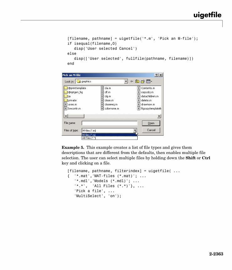
uigetfile
2-2363
[filename, pathname] = uigetfile('*.m', 'Pick an M-file');if isequal(filename,0) disp('User selected Cancel')else disp(['User selected', fullfile(pathname, filename)])end
Example 5. This example creates a list of file types and gives them descriptions that are different from the defaults, then enables multiple file selection. The user can select multiple files by holding down the Shift or Ctrl key and clicking on a file.
[filename, pathname, filterindex] = uigetfile( ... '*.mat','MAT-files (*.mat)'; ... '*.mdl','Models (*.mdl)'; ... '*.*', 'All Files (*.*)', ... 'Pick a file', ... 'MultiSelect', 'on');

uigetfile
2-2364
See Also uiputfile, uigetdir

uiimport
2-2365
2uiimportPurpose Open Import Wizard, the graphical user interface to import data
Syntax uiimportuiimport(filename)uiimport('-file')uiimport('-pastespecial')S = uiimport(...)
Description uiimport starts the Import Wizard in the current directory, presenting options to load data from a file or the clipboard.
uiimport(filename) starts the Import Wizard, opening the file specified in filename. The Import Wizard displays a preview of the data in the file.
uiimport('-file') works as above but presents the file selection dialog first.
uiimport('-pastespecial') works as above but presents the clipboard contents first.
S = uiimport(...) works as above with resulting variables stored as fields in the struct S.
Note For ASCII data, you must verify that the Import Wizard correctly identified the column delimiter.
See Also load, clipboard

uimenu
2-2366
2uimenuPurpose Create menus on figure windows
Syntax uimenu('PropertyName',PropertyValue,...)uimenu(parent,'PropertyName',PropertyValue,...)handle = uimenu('PropertyName',PropertyValue,...)handle = uimenu(parent,'PropertyName',PropertyValue,...)
Description uimenu creates a hierarchy of menus and submenus that are displayed in the figure window’s menu bar. You can also use uimenu to create menu items for context menus.
handle = uimenu('PropertyName',PropertyValue,...) creates a menu in the current figure’s menu bar using the values of the specified properties and assigns the menu handle to handle.
handle = uimenu(parent,'PropertyName',PropertyValue,...) creates a submenu of a parent menu or a menu item on a context menu specified by parent and assigns the menu handle to handle. If parent refers to a figure instead of another uimenu object or a uicontextmenu, MATLAB creates a new menu on the referenced figure’s menu bar.
Remarks MATLAB adds the new menu to the existing menu bar. Each menu choice can itself be a menu that displays its submenu when selected.
uimenu accepts property name/property value pairs, as well as structures and cell arrays of properties as input arguments. The uimenu Callback property defines the action taken when you activate the menu item. uimenu optionally returns the handle to the created uimenu object.
Uimenus only appear in figures whose WindowStyle is normal. If a figure containing uimenu children is changed to WindowStyle modal, the uimenu children still exist and are contained in the Children list of the figure, but are not displayed until the WindowStyle is changed to normal.
The value of the figure MenuBar property affects the location of the uimenu on the figure menu bar. When MenuBar is figure, a set of built-in menus precedes the uimenus on the menu bar (MATLAB controls the built-in menus and their handles are not available to the user). When MenuBar is none, uimenus are the only items on the menu bar (that is, the built-in menus do not appear).
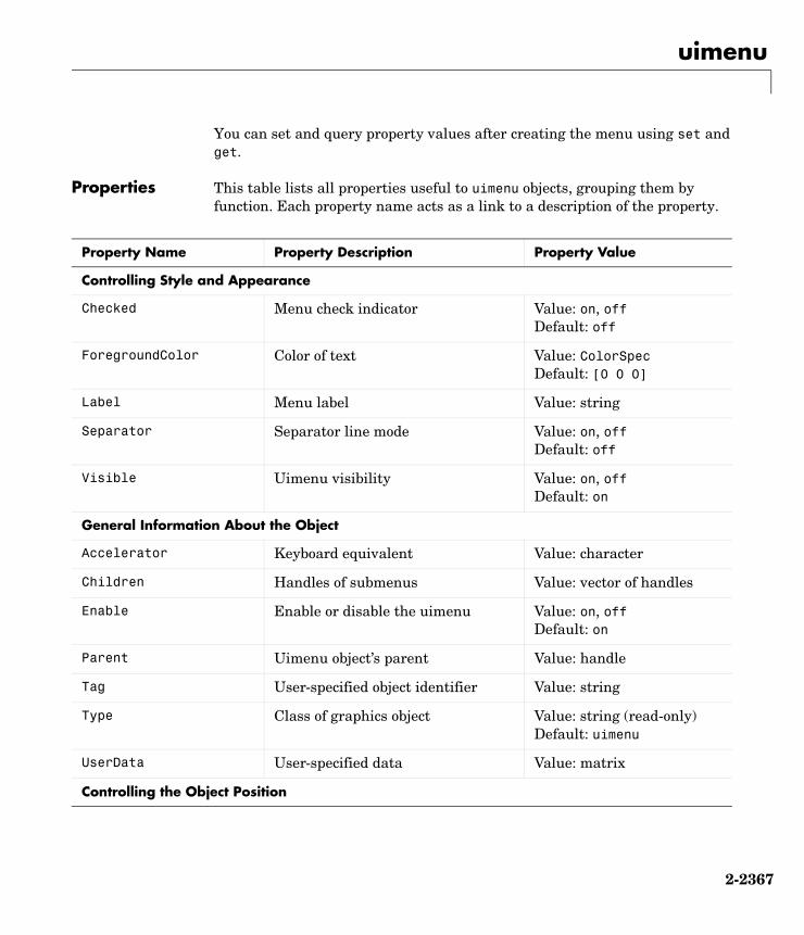
uimenu
2-2367
You can set and query property values after creating the menu using set and get.
Properties This table lists all properties useful to uimenu objects, grouping them by function. Each property name acts as a link to a description of the property.
Property Name Property Description Property Value
Controlling Style and Appearance
Checked Menu check indicator Value: on, offDefault: off
ForegroundColor Color of text Value: ColorSpecDefault: [0 0 0]
Label Menu label Value: string
Separator Separator line mode Value: on, offDefault: off
Visible Uimenu visibility Value: on, offDefault: on
General Information About the Object
Accelerator Keyboard equivalent Value: character
Children Handles of submenus Value: vector of handles
Enable Enable or disable the uimenu Value: on, offDefault: on
Parent Uimenu object’s parent Value: handle
Tag User-specified object identifier Value: string
Type Class of graphics object Value: string (read-only)Default: uimenu
UserData User-specified data Value: matrix
Controlling the Object Position

uimenu
2-2368
Examples This example creates a menu labeled Workspace whose choices allow users to create a new figure window, save workspace variables, and exit out of MATLAB. In addition, it defines an accelerator key for the Quit option.
f = uimenu('Label','Workspace');uimenu(f,'Label','New Figure','Callback','figure');uimenu(f,'Label','Save','Callback','save');uimenu(f,'Label','Quit','Callback','exit',...
'Separator','on','Accelerator','Q');
See Also uicontrol, uicontextmenu, gcbo, set, get, figure
Position Relative uimenu position Value: scalarDefault: [1]
Controlling Callback Routine Execution
BusyAction Callback routine interruption Value: cancel, queueDefault: queue
Callback Control action Value: string
CreateFcn Callback routine executed during object creation
Value: string
DeleteFcn Callback routine executed during object deletion
Value: string
Interruptible Callback routine interruption mode Value: on, offDefault: on
Controlling Access to Objects
HandleVisibility Whether handle is accessible from command line and GUIs
Value: on, callback, offDefault: on
Property Name Property Description Property Value

Uimenu Properties
2-2369
2Uimenu PropertiesModifying Properties
You can set and query graphics object properties in two ways:
• The Property Inspector is an interactive tool that enables you to see and change object property values. The Property inspector is available from GUIDE, or use the inspect function at the command line.
• The set and get commands enable you to set and query the values of properties
You can set default Uimenu properties on the root, figure and menu levels:
set(0,'DefaultUimenuPropertyName',PropertyValue...)set(gcf,'DefaultUimenuPropertyName',PropertyValue...)set(menu_handle,'DefaultUimenuPropertyName',PropertyValue...)
Where PropertyName is the name of the Uimenu property and PropertyValue is the value you specify as the default for that property.
For more information about changing the default value of property see Setting Default Property Values.
Uimenu Properties
This section lists all properties useful to uimenu objects along with valid values and instructions for their use. Curly braces enclose default values.
Property Name Property Description
Accelerator Keyboard equivalent
BusyAction Callback routine interruption
Callback Control action
Checked Menu check indicator
Children Handles of submenus
CreateFcn Callback routine executed during object creation
DeleteFcn Callback routine executed during object deletion
Enable Enable or disable the uimenu

Uimenu Properties
2-2370
Accelerator character
Keyboard equivalent. A character specifying the keyboard equivalent for the menu item. This allows users to select a particular menu choice by pressing the specified character in conjunction with another key, instead of selecting the menu item with the mouse. The key sequence is platform specific:
• For Microsoft Windows systems, the sequence is Ctrl+Accelerator. These keys are reserved for default menu items: c, v, and x.
• For UNIX systems, the sequence is Ctrl+Accelerator. These keys are reserved for default menu items: o, p, s, and w.
You can define an accelerator only for menu items that do not have children menus. Accelerators work only for menu items that directly execute a callback routine, not items that bring up other menus.
Note that the menu item does not have to be displayed (e.g., a submenu) for the accelerator key to work. However, the window focus must be in the figure when the key sequence is entered.
ForegroundColor Color of text
HandleVisibility Whether handle is accessible from command line and GUIs
Interruptible Callback routine interruption mode
Label Menu label
Parent Uimenu object’s parent
Position Relative uimenu position
Separator Separator line mode
Tag User-specified object identifier
Type Class of graphics object
UserData User-specified data
Visible Uimenu visibility
Property Name Property Description

Uimenu Properties
2-2371
To remove an accelerator, set Accelerator to an empty string, ''.
BusyAction cancel | queue
Callback routine interruption. If a callback is executing and the user triggers an event (such as a mouse click) on an object for which a callback is defined, the callback associated with the new event uses the value of BusyAction to decide whether or not to attempt to interrupt the executing callback.
• If the value is cancel, the event is discarded and the second callback does not execute.
• If the value is queue, and the Interruptible property of the first callback is on, the second callback is added to the event queue and executes in its turn after the first callback finishes execution.
Note If the interrupting callback is a DeleteFcn or CreateFcn callback or a figure’s CloseRequest or ResizeFcn callback, it interrupts an executing callback regardless of the value of that object’s Interruptible property. See the Interruptible property for information about controlling a callback’s interruptibility.
Callback string
Menu action. A callback routine that executes whenever you select the menu. Define this routine as a string that is a valid MATLAB expression or the name of an M-file. The expression executes in the MATLAB workspace.
A menu with children (submenus) executes its callback routine before displaying the submenus. A menu without children executes its callback routine when you release the mouse button (i.e., on the button up event).
Checked on | off
Menu check indicator. Setting this property to on places a check mark next to the corresponding menu item. Setting it to off removes the check mark. You can use this feature to create menus that indicate the state of a particular option. For example, suppose you have a menu item called Show axes that toggles the visibility of an axes between visible and invisible each time the user selects the menu item. If you want a check to appear next to the menu item

Uimenu Properties
2-2372
when the axes are visible, add the following code to the callback for the Show axes menu item:
if strcmp(get(gcbo, 'Checked'),'on') set(gcbo, 'Checked', 'off');else set(gcbo, 'Checked', 'on');end
This changes the value of the Checked property of the menu item from on to off or vice versa each time a user selects the menu item.
Note that there is no formal mechanism for indicating that an unchecked menu item will become checked when selected. Also, this property does not display the check mark on top level menus or submenus, although you can change the value of the property for these menus.
Note the following platform differences:
• On UNIX, the check mark is not displayed on submenus that have submenus.
• On Windows, the check mark is displayed on submenus, whether or not they have submenus.
Children vector of handles
Handles of submenus. A vector containing the handles of all children of the uimenu object. The children objects of uimenus are other uimenus, which function as submenus. You can use this property to reorder the menus.
CreateFcn string or function handle
Callback routine executed during object creation. The specified function executes when MATLAB creates a uimenu object. MATLAB sets all property values for the uimenu before executing the CreateFcn callback so these values are available to the callback. Within the function, use gcbo to get the handle of the uimenu being created.
Setting this property on an existing uimenu object has no effect.
You can define a default CreateFcn callback for all new uimenus. This default applies unless you override it by specifying a different CreateFcn callback when you call uimenu. For example, the code

Uimenu Properties
2-2373
set(0,'DefaultUimenuCreateFcn','set(gcbo,... ''Visible'',''on'')')
creates a default CreateFcn callback that runs whenever you create a new menu. It sets the default Visible property of a uimenu object.
To override this default and create a menu whose Visible property is set to a different value, call uimenu with code similar to
hpt = uimenu(...,'CreateFcn','set(gcbo,...''Visible'',''off'')')
Note To override a default CreateFcn callback you must provide a new callback and not just provide different values for the specified properties. This is because the CreateFcn callback runs after the property values are set, and can override property values you have set explicitly in the uimenu call. In the example above, if instead of redefining the CreateFcn property for this uimenu, you had explicitly set Visible to off, the default CreateFcn callback would have set Visible back to the default, i.e., on.
See Function Handle Callbacks for information on how to use function handles to define a callback function.
DeleteFcn string or function handle
Delete uimenu callback routine. A callback routine that executes when you delete the uimenu object (e.g., when you issue a delete command or cause the figure containing the uimenu to reset). MATLAB executes the routine before destroying the object’s properties so these values are available to the callback routine.
The handle of the object whose DeleteFcn is being executed is accessible only through the root CallbackObject property, which is more simply queried using gcbo.
See Function Handle Callbacks for information on how to use function handles to define a callback function.

Uimenu Properties
2-2374
Enable on | off
Enable or disable the uimenu. This property controls whether a menu item can be selected. When not enabled (set to off), the menu Label appears dimmed, indicating the user cannot select it.
ForegroundColor ColorSpec X-Windows only
Color of menu label string. This property determines color of the text defined for the Label property. Specify a color using a three-element RGB vector or one of the MATLAB predefined names. The default text color is black. See ColorSpec for more information on specifying color.
HandleVisibility on | callback | off
Control access to object’s handle. This property determines when an object’s handle is visible in its parent’s list of children. When a handle is not visible in its parent’s list of children, it is not returned by functions that obtain handles by searching the object hierarchy or querying handle properties. This includes get, findobj, gca, gcf, gco, newplot, cla, clf, and close. Neither is the handle visible in the parent figure’s CurrentObject property. Handles that are hidden are still valid. If you know an object’s handle, you can set and get its properties, and pass it to any function that operates on handles.
• Handles are always visible when HandleVisibility is on.
• Setting HandleVisibility to callback causes handles to be visible from within callback routines or functions invoked by callback routines, but not from within functions invoked from the command line. This provides a means to protect GUIs from command-line users, while allowing callback routines to have complete access to object handles.
• Setting HandleVisibility to off makes handles invisible at all times. This may be necessary when a callback routine invokes a function that might potentially damage the GUI (such as evaluating a user-typed string), and so temporarily hides its own handles during the execution of that function.
You can set the root ShowHiddenHandles property to on to make all handles visible, regardless of their HandleVisibility settings. This does not affect the values of the HandleVisibility properties.
Interruptible on | off
Callback routine interruption mode. If a callback is executing and the user triggers an event (such as a mouse click) on an object for which a callback is

Uimenu Properties
2-2375
defined, that callback attempts to interrupt the first callback. MATLAB processes the callbacks according to these factors:
• The Interruptible property of the object whose callback is executing
• Whether the executing callback contains drawnow, figure, getframe, pause, or waitfor statements
• The BusyAction property of the object whose callback is waiting to execute
If the Interruptible property of the object whose callback is executing is on (the default), the callback can be interrupted. Whenever the callback calls one of the drawnow, figure, getframe, pause, or waitfor functions, the function processes any events in the event queue, including the waiting callback, before performing its defined task.
If the Interruptible property of the object whose callback is executing is off, the callback cannot be interrupted (except by certain callbacks; see the note below). The BusyAction property of the object whose callback is waiting to execute determines what happens to the callback.
Note If the interrupting callback is a DeleteFcn or CreateFcn callback or a figure’s CloseRequest or ResizeFcn callback, it interrupts an executing callback regardless of the value of that object’s Interruptible property. The interrupting callback starts execution at the next drawnow, figure, getframe, pause, or waitfor statement. A figure’s WindowButtonDownFcn callback routine, or an object’s ButtonDownFcn or Callback routine are processed according to the rules described above.
Label string
Menu label. A string specifying the text label on the menu item. You can specify a mnemonic using the “&” character. Whatever character follows the “&” in the string appears underlined and selects the menu item when you type that character while the menu is visible. The “&” character is not displayed. To display the “&” character in a label, use two “&” characters in the string:
O&pen selection' yields Open selection
Save && Go' yields Save & Go

Uimenu Properties
2-2376
Parent handle
Uimenu’s parent. The handle of the uimenu’s parent object. The parent of a uimenu object is the figure on whose menu bar it displays, or the uimenu of which it is a submenu. You can move a uimenu object to another figure by setting this property to the handle of the new parent.
Position scalar
Relative menu position. The value of Position indicates placement on the menu bar or within a menu. Top-level menus are placed from left to right on the menu bar according to the value of their Position property, with 1 representing the left-most position. The individual items within a given menu are placed from top to bottom according to the value of their Position property, with 1 representing the top-most position.
Separator on | off
Separator line mode. Setting this property to on draws a dividing line above the menu item.
Tag string
User-specified object label. The Tag property provides a means to identify graphics objects with a user-specified label. This is particularly useful when constructing interactive graphics programs that would otherwise need to define object handles as global variables or pass them as arguments between callback routines. You can define Tag as any string.
Type string (read only)
Class of graphics object. For uimenu objects, Type is always the string 'uimenu'.
UserData matrix
User-specified data. Any matrix you want to associate with the uimenu object. MATLAB does not use this data, but you can access it using the set and get commands.
Visible on | off
Uimenu visibility. By default, all uimenus are visible. When set to off, the uimenu is not visible, but still exists and you can query and set its properties.

uint8, uint16, uint32, uint64
2-2377
2uint8, uint16, uint32, uint64Purpose Convert to unsigned integer
Syntax I = uint8(X)I = uint16(X)I = uint32(X)I = uint64(X)
Description I = uint*(X) converts the elements of array X into unsigned integers. X can be any numeric object (such as a double). The results of a uint* operation are shown in the next table.
double and single values are rounded to the nearest uint* value on conversion. A value of X that is above or below the range for an integer class is mapped to one of the endpoints of the range. For example,
uint16(70000)ans = 65535
If X is already an unsigned integer of the same class, then uint* has no effect.
You can define or overload your own methods for uint* (as you can for any object) by placing the appropriately named method in an @uint* directory within a directory on your path. Type help datatypes for the names of the methods you can overload.
Operation Output Range Output Type Bytes per Element
Output Class
uint8 0 to 255 Unsigned 8-bit integer
1 uint8
uint16 0 to 65,535 Unsigned 16-bit integer
2 uint16
uint32 0 to 4,294,967,295 Unsigned 32-bit integer
4 uint32
uint64 0 to 18,446,744,073,709,551,615 Unsigned 64-bit integer
8 uint64

uint8, uint16, uint32, uint64
2-2378
Remarks Most operations that manipulate arrays without changing their elements are defined for integer values. Examples are reshape, size, the logical and relational operators, subscripted assignment, and subscripted reference.
Some arithmetic operations are defined for integer arrays on interaction with other integer arrays of the same class (e.g., where both operands are uint16). Examples of these operations are +, -, .*, ./, .\ and .^. If at least one operand is scalar, then *, /, \, and ^ are also defined. Integer arrays may also interact with scalar double variables, including constants, and the result of the operation is an integer array of the same class. Integer arrays saturate on overflow in arithmetic.
A particularly efficient way to initialize a large array is by specifying the data type (i.e., class name) for the array in the zeros, ones, or eye function. For example, to create a 100-by-100 uint64 array initialized to zero, type
I = zeros(100, 100, 'uint64');
An easy way to find the range for any MATLAB integer type is to use the intmin and intmax functions as shown here for uint32:
intmin('uint32') intmax('uint32')ans = ans = 0 4294967295
See Also double, single, int8, int16, int32, int64, intmax, intmin

uiopen
2-2379
2uiopenPurpose Display a file selection dialog with appropriate file filters
Syntax uiopen
Description uiopen displays a file selection dialog from which a user can select a file to open. The dialog is the same as the one displayed when you select Open from the File menu in the MATLAB desktop.
Selecting a file in the dialog and clicking Open does the following:
• Gets the file using uigetfile
• Opens the file in the base workspace using the open command
Note uiopen cannot be compiled. If you want to create a file selection dialog that can be compiled, use uigetfile.
uiopen, or uiopen('MATLAB') displays the dialog with the file filter set to all MATLAB files.
uiopen('LOAD') displays the dialog with the file filter set to MAT-files (*.mat).
uiopen('FIGURE') displays the dialog with the file filter set to figure files (*.fig).
uiopen('SIMULINK') displays the dialog with the file filter set to model files (*.mdl).
uiopen('EDITOR') displays the dialog with the file filter set to all MATLAB files except for MAT-files and FIG-files. All files are opened in the MATLAB Editor.
See Also uigetfile, uiputfile, uisave

uipanel
2-2380
2uipanelPurpose Uipanel container object
Syntax h = uipanel('PropertyName1',value1,'PropertyName2',value2,...)
Description A uipanel groups components. It can contain user interface controls with which the user interacts directly. It can also contain axes, other uipanels, and uibuttongroups. It cannot contain ActiveX controls.
h = uipanel creates a uipanel container object in a figure, uipanel, or uibuttongroup. Use the Parent property to specify the parent figure, uipanel, or uibuttongroup. If you do not specify a parent, uipanel adds the panel to the current figure. If no figure exists, one is created.
A uipanel object can have axes, uicontrol, uipanel, and uibuttongroup objects as children. For the children of a uipanel, the Position property is interpreted relative to the uipanel. If you move the panel, the children automatically move with it and maintain their positions relative to the panel.
After creating a uipanel object, you can set and query its property values using set and get.
Properties This table lists all properties useful to uipanel objects, grouping them by function. Each property name acts as a link to a description of the property. Curly braces denote the default value, if any
Property Name Description Property Value
Controlling Style and Appearance
BackgroundColor Color of the uipanel background
ColorSpec. Default is the same as the default uicontrol background.
BorderType Type of border around the uipanel area.
[none|etchedin|etchedout|beveledin|beveledout|line]
BorderWidth Width of the panel border. Integer. Default is 1.

uipanel
2-2381
Clipping Clipping of child axes, uipanels, and uibuttongroups to the uipanel. Does not affect child uicontrols.
[on|off]
ForegroundColor Title font color and/or color of 2-D border line
ColorSpec. Default is [0 0 0] (black).
HighlightColor 3-D frame highlight color ColorSpec. Default is [1 1 1] (white).
SelectionHighlight Object highlighted when selected
[on|off]
ShadowColor 3-D frame shadow color ColorSpec. Default is [.5 .5 .5] (grey).
Visible Uipanel visibility. Note: Controls the Visible property of child axes, uibuttongroups. and uipanels. Does not affect child uicontrols.
[on|off]
General Information About the Object
Children All children of the uipanel Vector of handles
Parent Uipanel object’s parent Figure, uipanel, or uibuttongroup handle
Selected Whether object is selected [on|off]
Tag User-specified object identifier
String
UserData User-specified data Matrix
Property Name Description Property Value

uipanel
2-2382
Controlling the Object Position
Position Panel position relative to parent figure, uipanel, or uibuttongroup
Position spec [x y w h]. Default is [0 0 1 1]
Units Units usd to interpret the position vector
[inches|centimeters|normalized|points|pixels|characters]
Controlling Fonts and Labels
FontAngle Title font angle [normal|italic|oblique]
FontName Title font name String. Default is system dependent.
FontSize Title font size Integer. Default is system dependent.
FontUnits Title font units [inches|centimeters|normalized|points|pixels]
FontWeight Title font weight [light|normal|demi|bold]
Title Title string String
TitlePosition Location of title string in relation to the panel
[lefttop|centertop|righttop|leftbottom|centerbottom|rightbottom]
Controlling Callback Routine Execution
BusyAction Interruption of other callback routines
[queue|cancel]
ButtonDownFcn Button-press callback routine
String or function handle
Property Name Description Property Value

uipanel
2-2383
Examples This example creates a uipanel in a figure, then creates a subpanel in the first panel. Finally, it adds a pushbutton to the subpanel. Both panels use the default Units property value, normalized. Note that default Units for the uicontrol pushbutton is pixels.
h = figure;hp = uipanel('Title','Main Panel','FontSize',12,... 'BackgroundColor','white',... 'Position',[.25 .1 .67 .67]);hsp = uipanel('Parent',hp,'Title','Subpanel','FontSize',12,... 'Position',[.4 .1 .5 .5]);hbsp = uicontrol('Parent',hsp,'String','Push here',... 'Position',[18 18 72 36]);
CreateFcn Callback routine executed during object creation
String or function handle
DeleteFcn Callback routine executed during object deletion
String or function handle
Interruptible Callback routine interruption mode
[on|off]
ResizeFcn User-specified resize routine
String or function handle
UIContextMenu Associates a uicontextmenu with the uipanel
Handle
Controlling Access to Objects
HandleVisibility Handle accessibility from commandline and GUIs
[on|callback|off]
HitTest Selectable by mouse click [on|off]
Property Name Description Property Value

uipanel
2-2384
See Also hgtransform, uibuttongroup, uicontrol

Uipanel Properties
2-2385
2Uipanel PropertiesModifying Properties
You can set and query graphics object properties in two ways:
• The Property Inspector is an interactive tool that enables you to see and change object property values. The Property inspector is available from GUIDE, or use the inspect function at the command line.
• The set and get functions enable you to set and query the values of properties.
You can set default uipanel properties by typing:
set(h,'DefaultUipanelPropertyName',PropertyValue...)
Where h can be the root handle (0), a figure handle, or a uipanel handle. PropertyName is the name of the uipanel property and PropertyValue is the value you specify as the default for that property.
Note Default properties you set for uipanels also apply to uibuttongroups.
For more information about changing the default value of a property see Setting Default Property Values. For an example, see the CreateFcn property.
Uipanel Properties
This section lists all properties useful to uipanel objects along with valid values and a descriptions of their use. Curly braces enclose default values.
Property Name Description
BackgroundColor Color of the uipanel background
BorderType Type of border around the uipanel area.
BorderWidth Width of the panel border.
BusyAction Interruption of other callback routines
ButtonDownFcn Button-press callback routine
Children All children of the uipanel

Uipanel Properties
2-2386
Clipping Clipping of child axes, uipanels, and uibuttongroups to the uipanel. Does not affect child uicontrols.
CreateFcn Callback routine executed during object creation
DeleteFcn Callback routine executed during object deletion
FontAngle Title font angle
FontName Title font name
FontSize Title font size
FontUnits Title font units
FontWeight Title font weight
ForegroundColor Title font color and/or color of 2-D border line
HandleVisibility Handle accessibility from commandline and GUIs
HighlightColor 3-D frame highlight color
HitTest Selectable by mouse click
Interruptible Callback routine interruption mode
Parent Uipanel object’s parent
Position Panel position relative to parent figure or uipanel
ResizeFcn User-specified resize routine
Selected Whether object is selected
SelectionHighlight Object highlighted when selected
ShadowColor 3-D frame shadow color
Tag User-specified object identifier
Title Title string
TitlePosition Location of title string in relation to the panel
Property Name Description

Uipanel Properties
2-2387
BackgroundColor ColorSpec
Color of the uipanel background. A three-element RGB vector or one of the MATLAB predefined names, specifying the background color. See the ColorSpec reference page for more information on specifying color.
BorderType none | etchedin | etchedout |beveledin | beveledout | line
Border of the uipanel area. Used to define the panel area graphically. Etched and beveled borders provide a 3-D look. Use the HighlightColor and ShadowColor properties to specify the border color of etched and beveled borders. A line border is 2-D. Use the ForegroundColor property to specify its color.
BorderWidth integer
Width of the panel border. The width of the panel borders in pixels. The default border width is 1 pixel. 3-D borders wider than 3 may not appear correctly at the corners.
BusyAction cancel | queue
Callback routine interruption. If a callback is executing and the user triggers an event (such as a mouse click) on an object for which a callback is defined, the callback associated with the new event uses the value of BusyAction to decide whether or not to attempt to interrupt the executing callback.
• If the value is cancel, the event is discarded and the second callback does not execute.
UIContextMenu Associates uicontext menu with the uipanel
Units Units used to interpret the position vector
UserData User-specified data
Visible Uipanel visibility. Note: Controls the Visible property of child axes, uibuttongroups. and uipanels. Does not affect child uicontrols.
Property Name Description

Uipanel Properties
2-2388
• If the value is queue, and the Interruptible property of the first callback is on, the second callback is added to the event queue and executes in its turn after the first callback finishes execution.
Note If the interrupting callback is a DeleteFcn or CreateFcn callback or a figure’s CloseRequest or ResizeFcn callback, it interrupts an executing callback regardless of the value of that object’s Interruptible property. See the Interruptible property for information about controlling a callback’s interruptibility.
ButtonDownFcn string or function handle
Button-press callback routine. A callback routine that executes when you press a mouse button while the pointer is in a 5-pixel wide border around the uipanel. This is useful for implementing actions to interactively modify control object properties, such as size and position, when they are clicked on (using the selectmoveresize function, for example).
If you define this routine as a string, the string can be a valid MATLAB expression or the name of an M-file. The expression executes in the MATLAB workspace.
Children vector of handles
Children of the uipanel. A vector containing the handles of all children of the uipanel. A uipanel object’s children are axes, uipanels, uibuttongroups, and uicontrols. You can use this property to reorder the children.
Clipping on | off
Clipping mode. By default, MATLAB clips a uipanel’s child axes, uipanels, and uibuttongroups to the uipanel rectangle. If you set Clipping to off, the axis, uipanel, or uibuttongroup is displayed outside the panel rectangle. This property does not affect child uicontrols which, by default, can display outside the panel rectangle.
CreateFcn string or function handle
Callback routine executed during object creation. The specified function executes when MATLAB creates a uipanel object. MATLAB sets all property values for the uipanel before executing the CreateFcn callback so these values

Uipanel Properties
2-2389
are available to the callback. Within the function, use gcbo to get the handle of the uipanel being created.
Setting this property on an existing uipanel object has no effect.
You can define a default CreateFcn callback for all new uipanels. This default applies unless you override it by specifying a different CreateFcn callback when you call uipanel. For example, the code
set(0,'DefaultUipanelCreateFcn','set(gcbo,... ''FontName'',''arial'',''FontSize'',12)')
creates a default CreateFcn callback that runs whenever you create a new panel. It sets the default font name and font size of the uipanel title.
Note Uibuttongroup takes its default property values from uipanel. Defining a default property for all uipanels defines the same default property for all uibuttongroups.
To override this default and create a panel whose FontName and FontSize properties are set to different values, call uipanel with code similar to
hpt = uipanel(...,'CreateFcn','set(gcbo,...''FontName'',''times'',''FontSize'',14)')
Note To override a default CreateFcn callback you must provide a new callback and not just provide different values for the specified properties. This is because the CreateFcn callback runs after the property values are set, and can override property values you have set explicitly in the uipushtool call. In the example above, if instead of redefining the CreateFcn property for this uipanel, you had explicitly set Fontsize to 14, the default CreateFcn callback would have set FontSize back to the system dependent default.
See Function Handle Callbacks for information on how to use function handles to define a callback function.
Uipanel Properties
2-2390
DeleteFcn string or function handle
Callback routine executed during object deletion. A callback routine that executes when you delete the uipanel object (e.g., when you issue a delete command or clear the figure containing the uipanel). MATLAB executes the routine before destroying the object's properties so these values are available to the callback routine. The handle of the object whose DeleteFcn is being executed is accessible only through the root CallbackObject property, which you can query using gcbo.
FontAngle normal | italic | oblique
Character slant used in the Title. MATLAB uses this property to select a font from those available on your particular system. Setting this property to italic or oblique selects a slanted version of the font, when it is available on your system.
FontName string
Font family used in the Title. The name of the font in which to display the Title. To display and print properly, this must be a font that your system supports. The default font is system dependent. To eliminate the need to hard code the name of a fixed-width font, which may not display text properly on systems that do not use ASCII character encoding (such as in Japan), set FontName to the string FixedWidth (this string value is case insensitive).
set(uicontrol_handle,'FontName','FixedWidth')
This then uses the value of the root FixedWidthFontName property which can be set to the appropriate value for a locale from startup.m in the end user's environment. Setting the root FixedWidthFontName property causes an immediate update of the display to use the new font
FontSize integer
Title font size. A number specifying the size of the font in which to display the Title, in units determined by the FontUnits property. The default size is system dependent.
FontUnits inches | centimeters | normalized | points |pixels
Title font size units. Normalized units interpret FontSize as a fraction of the height of the uipanel. When you resize the uipanel, MATLAB modifies the

Uipanel Properties
2-2391
screen FontSize accordingly. pixels, inches, centimeters, and points are absolute units (1 point = 1/72 inch).
FontWeight light | normal | demi | bold
Weight of characters in the title. MATLAB uses this property to select a font from those available on your particular system. Setting this property to bold causes MATLAB to use a bold version of the font, when it is available on your system.
ForegroundColor ColorSpec
Color used for title font and 2-D border line. A three-element RGB vector or one of the MATLAB predefined names, specifying the font or line color. See the ColorSpec reference page for more information on specifying color.
HandleVisibility on | callback | off
Control access to object’s handle. This property determines when an object’s handle is visible in its parent’s list of children. When a handle is not visible in its parent’s list of children, it is not returned by functions that obtain handles by searching the object hierarchy or querying handle properties. This includes get, findobj, gca, gcf, gco, newplot, cla, clf, and close. Neither is the handle visible in the parent figure’s CurrentObject property. Handles that are hidden are still valid. If you know an object’s handle, you can set and get its properties, and pass it to any function that operates on handles.
• Handles are always visible when HandleVisibility is on.
• Setting HandleVisibility to callback causes handles to be visible from within callback routines or functions invoked by callback routines, but not from within functions invoked from the command line. This provides a means to protect GUIs from command-line users, while allowing callback routines to have complete access to object handles.
• Setting HandleVisibility to off makes handles invisible at all times. This may be necessary when a callback routine invokes a function that might potentially damage the GUI (such as evaluating a user-typed string), and so temporarily hides its own handles during the execution of that function.
You can set the root ShowHiddenHandles property to on to make all handles visible, regardless of their HandleVisibility settings. This does not affect the values of the HandleVisibility properties.
Uipanel Properties
2-2392
HighlightColor ColorSpec
3-D frame highlight color. A three-element RGB vector or one of the MATLAB predefined names, specifying the highlight color. See the ColorSpec reference page for more information on specifying color.
HitTest on | off
Selectable by mouse click. HitTest determines if the figure can become the current object (as returned by the gco command and the figure CurrentObject property) as a result of a mouse click on the figure. If HitTest is off, clicking the figure sets the CurrentObject to the empty matrix.
Interruptible on | off
Callback routine interruption mode. If a callback is executing and the user triggers an event (such as a mouse click) on an object for which a callback is defined, that callback attempts to interrupt the first callback. MATLAB processes the callbacks according to these factors:
• The Interruptible property of the object whose callback is executing
• Whether the executing callback contains drawnow, figure, getframe, pause, or waitfor statements
• The BusyAction property of the object whose callback is waiting to execute
If the Interruptible property of the object whose callback is executing is on (the default), the callback can be interrupted. Whenever the callback calls one of the drawnow, figure, getframe, pause, or waitfor functions, the function processes any events in the event queue, including the waiting callback, before performing its defined task.
If the Interruptible property of the object whose callback is executing is off, the callback cannot be interrupted (except by certain callbacks; see the note below). The BusyAction property of the object whose callback is waiting to execute determines what happens to the callback.
Note If the interrupting callback is a DeleteFcn or CreateFcn callback or a figure’s CloseRequest or ResizeFcn callback, it interrupts an executing callback regardless of the value of that object’s Interruptible property. The interrupting callback starts execution at the next drawnow, figure, getframe, pause, or waitfor statement. A figure’s WindowButtonDownFcn callback

Uipanel Properties
2-2393
routine, or an object’s ButtonDownFcn or Callback routine are processed according to the rules described above.
Parent handle
Uipanel parent. The handle of the uipanel’s parent figure, uipanel, or uibuttongroup. You can move a uipanel object to another figure, uipanel, or uibuttongroup by setting this property to the handle of the new parent.
Position position rectangle
Size and location of uipanel relative to parent. The rectangle defined by this property specifies the size and location of the panel within the parent figure window, uipanel, or uibuttongroup. Specify Position as
[left bottom width height]
left and bottom are the distance from the lower-left corner of the parent object to the lower-left corner of the uipanel object. width and height are the dimensions of the uipanel rectangle, including the title. All measurements are in units specified by the Units property.
ResizeFcn string or function handle
Resize callback routine. MATLAB executes this callback routine whenever a user resizes the uipanel and the figure Resize property is set to on, or in GUIDE, the Resize behavior option is set to Other. You can query the uipanel Position property to determine its new size and position. During execution of the callback routine, the handle to the figure being resized is accessible only through the root CallbackObject property, which you can query using gcbo.
You can use ResizeFcn to maintain a GUI layout that is not directly supported by the MATLAB Position/Units paradigm.
See Function Handle Callbacks for information on how to use function handles to define the callback function.
See Resize Behavior for information on creating resize functions using GUIDE.
Selected on | off (read only)
Is object selected? This property indicates whether the figure is selected. When this property is on, MATLAB displays selection handles if the SelectionHighlight property is also on. You can, for example, define the
Uipanel Properties
2-2394
ButtonDownFcn to set this property, allowing users to select the object with the mouse.
SelectionHighlight on | off
Object highlighted when selected. When the Selected property is on, MATLAB indicates the selected state by drawing four edge handles and four corner handles. When SelectionHighlight is off, MATLAB does not draw the handles.
ShadowColor ColorSpec
3-D frame shadow color. A three-element RGB vector or one of the MATLAB predefined names, specifying the shadow color. See the ColorSpec reference page for more information on specifying color.
Tag string
User-specified object identifier. The Tag property provides a means to identify graphics objects with a user-specified label. You can define Tag as any string.
With the findobj function, you can locate an object with a given Tag property value. This saves you from defining object handles as global variables. For example, this function call returns the handles of all children (of the specified figures) that have the Tag value 'FormatTb'.
h = findobj(figurehandles,'Tag','FormatTb')
Title string
Title string. The text displayed in the panel title. You can position the title using the TitlePosition property.
If the string value is specified as a cell array of strings or padded string matrix, only the first string of a cell array or of a padded string matrix is displayed; the rest are ignored. Vertical slash ('|') characters are not interpreted as line breaks and instead show up in the text displayed in the uipanel title.
Setting a property value to default, remove, or factory produces the effect described in Setting Default Values. To set Title to one of these words, you must precede the word with the backslash character. For example,
hp = uipanel(...,'Title','\Default');

Uipanel Properties
2-2395
TitlePosition lefttop | centertop | righttop |leftbottom | centerbottom | rightbottom
Location ofthe title. This property determines the location of the title string, in relation to the uipanel.
UIContextMenu handle
Associate a context menu with a uipanel. Assign this property the handle of a Uicontextmenu object. MATLAB displays the context menu whenever you right-click the uipanel. Use the uicontextmenu function to create the context menu.
Units inches | centimeters | normalized |points | pixels | characters
Units of measurement. MATLAB uses these units to interpret the Position property. All units are measured from the lower-left corner of the figure window.
• Normalized units map the lower-left corner of the figure window to (0,0) and the upper-right corner to (1.0,1.0).
• pixels, inches, centimeters, and points are absolute units (1 point = 1/72 inch).
• Character units are characters using the default system font; the width of one character is the width of the letter x, the height of one character is the distance between the baselines of two lines of text.
If you change the value of Units, it is good practice to return it to its default value after completing your computation so as not to affect other functions that assume Units is set to the default value.
UserData matrix
User-specified data. Any data you want to associate with the uipanel object. MATLAB does not use this data, but you can access it using set and get.
Visible on | off
Uipanel visibility. By default, a uipanel object is visible. When set to off, the uipanel is not visible, but still exists and you can query and set its properties.

Uipanel Properties
2-2396
Note The value of a uipanel’s Visible property also controls the Visible property of child axes, uipanels, and uibuttongroups. This property does not affect the Visible property of child uicontrols.

uipushtool
2-2397
2uipushtoolPurpose Create a push button on the current or specified toolbar
Syntax htt = uipushtool('PropertyName1',value1,...'PropertyName2',value2,...)
htt = uipushtool(ht,...)
Description uipushtool('PropertyName1',value1,'PropertyName2',value2,...)creates a push button on the uitoolbar at the top of the current figure window, and returns a handle to it. uipushtool assigns the specified property values, and assigns default values to the remaining properties. You can change the property values at a later time using the set function.
Type get(htt) to see a list of uipushtool object properties and their current values. Type set(htt) to see a list of uipushtool object properties that you can set and their legal property values. See the Uipushtool Properties reference page for more information.
uipushtool(ht,...) creates a button with ht as a parent. ht must be a uitoolbar handle.
Remarks uipushtool accepts property name/property value pairs, as well as structures and cell arrays of properties as input arguments.
Uipushtools only appear in figures whose WindowStyle is normal. If a figure containing a uitoolbar and its uipushtool children is changed to WindowStyle modal, the uipushtools still exist and are contained in the Children list of the uitoolbar, but are not displayed until the WindowStyle is changed to normal.
Properties This table lists all properties useful to uipushtool objects, grouping them by function. Each property name acts as a link to a more detailed description of the property.
Property Name Property Description Property Value
Controlling Style and Appearance
CData Truecolor image displayed on the uipushtool
Value: m-by-n-by-3 array

uipushtool
2-2398
Separator Separator line mode Value: on, offDefault: off
Visible Uipushtool visibility Value: on, offDefault: on
General Information About the Object
BeingDeleted This object is being deleted Value: on, off (read-only)Default: off
Enable Enable or disable the uipushtool Value: on, inactive, offDefault: on
Parent Uipushtool object’s parent toolbar. Value: handle
Tag User-specified object identifier Value: string
TooltipString Content of object’s tooltip Value: string
Type Class of graphics object Value: string (read-only)Default: uipushtool
UserData User-specified data Value: array
Controlling Callback Routine Execution
BusyAction Interruption of other callback routines
Value: cancel, queueDefault: queue
ClickedCallback Control action. Value: string or function handle
CreateFcn Callback routine executed during object creation
Value: string or function handle
DeleteFcn Callback routine executed during object deletion
Value: string or function handle
Interruptible Callback routine interruption mode Value: on, offDefault: on
Property Name Property Description Property Value

uipushtool
2-2399
Examples This example creates a uitoolbar object and places a uipushtool object on it.
h = figure('ToolBar','none')ht = uitoolbar(h)a = [.05:.05:0.95];b(:,:,1) = repmat(a,19,1)';b(:,:,2) = repmat(a,19,1);b(:,:,3) = repmat(flipdim(a,2),19,1);hpt = uipushtool(ht,'CData',b,'TooltipString','Hello')
Controlling Access to Objects
HandleVisibility Handle accessibility from command line and code associated with the GUIs.
Value: on, callback, offDefault: on
Property Name Property Description Property Value

uipushtool
2-2400
Object Hierarchy
See Also get, set, uicontrol, uitoggletool, uitoolbar
Root
UimenuAxes Uicontrol
Figure
Uicontextmenu
Uimenu Uimenu
Uitoolbar
Uipushtool Uitoggletool

Uipushtool Properties
2-2401
2Uipushtool PropertiesModifying Properties
You can set and query graphics object properties in two ways:
• The Property Inspector is an interactive tool that enables you to see and change object property values. The Property inspector is available from GUIDE, or use the inspect function at the command line.
• The set and get functions enable you to set and query the values of properties.
You can set default Uipushtool properties by typing:
set(h,'DefaultUipushtoolPropertyName',PropertyValue...)
Where h can be the root handle (0), a figure handle, a uitoolbar handle, or a uipushtool handle. PropertyName is the name of the Uipushtool property and PropertyValue is the value you specify as the default for that property.
For more information about changing the default value of a property see Setting Default Property Values.
Uipushtool Properties
This section lists all properties useful to uipushtool objects along with valid values and a descriptions of their use. Curly braces enclose default values.
Property Purpose
BeingDeleted This object is being deleted.
BusyAction Callback routine interruption.
CData Truecolor image displayed on the control.
ClickedCallback Control action.
CreateFcn Callback routine executed during object creation.
DeleteFcn Delete uipushtool callback routine.
Enable Enable or disable the uipushtool.
HandleVisibility Control access to object’s handle.
Interruptible Callback routine interruption mode.
Parent Handle of uipushtool’s parent.

Uipushtool Properties
2-2402
BeingDeleted on | off (read only)
This object is being deleted. The BeingDeleted property provides a mechanism that you can use to determine if objects are in the process of being deleted. MATLAB sets the BeingDeleted property to on when the object’s delete function callback is called (see the DeleteFcn property) It remains set to on while the delete function executes, after which the object no longer exists.
For example, some functions may not need to perform actions on objects that are being deleted, and therefore, can check the object’s BeingDeleted property before acting.
BusyAction cancel | queue
Callback routine interruption. If a callback is executing and the user triggers an event (such as a mouse click) on an object for which a callback is defined, the callback associated with the new event uses the value of BusyAction to decide whether or not to attempt to interrupt the executing callback.
• If the value is cancel, the event is discarded and the second callback does not execute.
• If the value is queue, and the Interruptible property of the first callback is on, the second callback is added to the event queue and executes in its turn after the first callback finishes execution.
Note If the interrupting callback is a DeleteFcn or CreateFcn callback or a figure’s CloseRequest or ResizeFcn callback, it interrupts an executing
Separator Separator line mode
Tag User-specified object label.
TooltipString Content of object’s tooltip.
Type Object class.
UserData User specified data.
Visible Uipushtool visibility.
Property (Continued) Purpose

Uipushtool Properties
2-2403
callback regardless of the value of that object’s Interruptible property. See the Interruptible property for information about controlling a callback’s interruptibility.
CData 3-dimensional array
Truecolor image displayed on control. An n-by-m-by-3 array of RGB values that defines a truecolor image displayed on either a push button or toggle button. Each value must be between 0.0 and 1.0. The largest image that fits on the push tool is 20-by-20. If the array is larger, only the center 20-by-20 part of the array is used.
ClickedCallback string or function handle
Control action. A routine that executes when the uipushtool’s Enable property is set to on, and you press a mouse button while the pointer is on the push tool itself or in a 5-pixel wide border around it.
CreateFcn string or function handle
Callback routine executed during object creation. The specified function executes when MATLAB creates a uipushtool object. MATLAB sets all property values for the uipushtool before executing the CreateFcn callback so these values are available to the callback. Within the function, use gcbo to get the handle of the push tool being created.
Setting this property on an existing uipushtool object has no effect.
You can define a default CreateFcn callback for all new uipushtools. This default applies unless you override it by specifying a different CreateFcn callback when you call uipushtool. For example, the code
imga(:,:,1) = rand(20);imga(:,:,2) = rand(20);imga(:,:,3) = rand(20);set(0,'DefaultUipushtoolCreateFcn','set(gcbo,''Cdata'',imga)'
creates a default CreateFcn callback that runs whenever you create a new push tool. It sets the default image imga on the push tool.
To override this default and create a push tool whose Cdata property is set to a different image, call uipushtool with code similar to

Uipushtool Properties
2-2404
a = [.05:.05:0.95];imgb(:,:,1) = repmat(a,19,1)';imgb(:,:,2) = repmat(a,19,1);imgb(:,:,3) = repmat(flipdim(a,2),19,1);hpt = uipushtool(...,'CreateFcn','set(gcbo,''CData'',imgb)',...)
Note To override a default CreateFcn callback you must provide a new callback and not just provide different values for the specified properties. This is because the CreateFcn callback runs after the property values are set, and can override property values you have set explicitly in the uipushtool call. In the example above, if instead of redefining the CreateFcn property for this push tool, you had explicitly set CData to imgb, the default CreateFcn callback would have set CData back to imga.
See Function Handle Callbacks for information on how to use function handles to define a callback function.
DeleteFcn string or function handle
Callback routine executed during object deletion. A callback routine that executes when you delete the uipushtool object (e.g., when you call the delete function or cause the figure containing the uipushtool to reset). MATLAB executes the routine before destroying the object’s properties so these values are available to the callback routine.
The handle of the object whose DeleteFcn is being executed is accessible only through the root CallbackObject property, which you can query using gcbo.
See Function Handle Callbacks for information on how to use function handles to define a callback function.
Enable on | off
Enable or disable the uipushtool. This property controls how uipushtools respond to mouse button clicks, including which callback routines execute.
• on – The uipushtool is operational (the default).
• off – The uipushtool is not operational and its image (set by the Cdata property) is grayed out.

Uipushtool Properties
2-2405
When you left-click on a uipushtool whose Enable property is on, MATLAB performs these actions in this order:
1 Sets the figure’s SelectionType property.
2 Executes the push tool’s ClickedCallback routine.
3 Does not set the figure’s CurrentPoint property and does not execute the figure’s WindowButtonDownFcn callback.
When you left-click on a uipushtool whose Enable property is off, or when you right-click a uipushtool whose Enable property has any value, MATLAB performs these actions in this order:
1 Sets the figure’s SelectionType property.
2 Sets the figure’s CurrentPoint property.
3 Executes the figure’s WindowButtonDownFcn callback.
4 Does not execute the push tool’s ClickedCallback routine.
HandleVisibility on | callback | off
Control access to object’s handle. This property determines when an object’s handle is visible in its parent’s list of children. When a handle is not visible in its parent’s list of children, it is not returned by functions that obtain handles by searching the object hierarchy or querying handle properties. This includes get, findobj, gca, gcf, gco, newplot, cla, clf, and close. Neither is the handle visible in the parent figure’s CurrentObject property. Handles that are hidden are still valid. If you know an object’s handle, you can set and get its properties, and pass it to any function that operates on handles.
• Handles are always visible when HandleVisibility is on.
• Setting HandleVisibility to callback causes handles to be visible from within callback routines or functions invoked by callback routines, but not from within functions invoked from the command line. This provides a means to protect GUIs from command-line users, while allowing callback routines to have complete access to object handles.
• Setting HandleVisibility to off makes handles invisible at all times. This may be necessary when a callback routine invokes a function that might potentially damage the GUI (such as evaluating a user-typed string), and so temporarily hides its own handles during the execution of that function.

Uipushtool Properties
2-2406
You can set the root ShowHiddenHandles property to on to make all handles visible, regardless of their HandleVisibility settings. This does not affect the values of the HandleVisibility properties.
Interruptible on | off
Callback routine interruption mode. If a callback is executing and the user triggers an event (such as a mouse click) on an object for which a callback is defined, that callback attempts to interrupt the first callback. MATLAB processes the callbacks according to these factors:
• The Interruptible property of the object whose callback is executing
• Whether the executing callback contains drawnow, figure, getframe, pause, or waitfor statements
• The BusyAction property of the object whose callback is waiting to execute
If the Interruptible property of the object whose callback is executing is on (the default), the callback can be interrupted. Whenever the callback calls one of the drawnow, figure, getframe, pause, or waitfor functions, the function processes any events in the event queue, including the waiting callback, before performing its defined task.
If the Interruptible property of the object whose callback is executing is off, the callback cannot be interrupted (except by certain callbacks; see the note below). The BusyAction property of the object whose callback is waiting to execute determines what happens to the callback.
Note If the interrupting callback is a DeleteFcn or CreateFcn callback or a figure’s CloseRequest or ResizeFcn callback, it interrupts an executing callback regardless of the value of that object’s Interruptible property. The interrupting callback starts execution at the next drawnow, figure, getframe, pause, or waitfor statement. A figure’s WindowButtonDownFcn callback routine, or an object’s ButtonDownFcn or Callback routine are processed according to the rules described above.

Uipushtool Properties
2-2407
Parent handle
Uipushtool parent. The handle of the uipushtool’s parent toolbar. You can move a uipushtool object to another toolbar by setting this property to the handle of the new parent.
Separator on | off
Separator line mode. Setting this property to on draws a dividing line to the left of the uipushtool.
Tag string
User-specified object identifier. The Tag property provides a means to identify graphics objects with a user-specified label. You can define Tag as any string.
With the findobj function, you can locate an object with a given Tag property value. This saves you from defining object handles as global variables. For example, this function call returns the handles of all children (of the specified toolbars) that have the Tag value 'Copy'.
h = findobj(uitoolbarhandles,'Tag','Copy')
TooltipString string
Content of tooltip for object. The TooltipString property specifies the text of the tooltip associated with the uipushtool. When the user moves the mouse pointer over the control and leaves it there, the tooltip is displayed.
Type string (read-only)
Object class. This property identifies the kind of graphics object. For uipushtool objects, Type is always the string 'uipushtool'.
UserData array
User specified data. You can specify UserData as any array you want to associate with the uipushtool object. The object does not use this data, but you can access it using the set and get functions.
Visible on | off
Uipushtool visibility. By default, all uipushtools are visible. When set to off, the uipushtool is not visible, but still exists and you can query and set its properties.

uiputfile
2-2408
2uiputfilePurpose Standard dialog box for saving files
Syntax uiputfileuiputfile('FilterSpec')uiputfile('FilterSpec','DialogTitle')uiputfile('FilterSpec','DialogTitle', 'DefaultName')uiputfile(...,'Location',[x y])[FileName,PathName] = uiputfile(...)[FileName,PathName,FilterIndex] = uiputfile(...)
Description uiputfile displays a dialog box used to select a file for saving. The dialog box lists the files and directories in the current directory.
uiputfile('FilterSpec') displays a dialog box that lists files in the current directory. FilterSpec determines what files are displayed initially in the dialog box. For example '*.m' lists all MATLAB M-files.
If FilterSpec is a string or cell array, uiputfile appends 'All Files' to the list of file types. If FilterSpec is a cell array, the first column is used as the list of extensions, and the second column is used as the list of descriptions. FilterSpec can also be a filename. In this case the filename becomes the default filename and the file’s extension is used as the default filter. If FilterSpec is not specified, uiputfile uses the default list of file types (i.e., all MATLAB files).
uiputfile('FilterSpec','DialogTitle') displays a dialog box that has the title DialogTitle. To use the default file types and specify a dialog title, enter
uiputfile('','DialogTitle')
uiputfile('FilterSpec','DialogTitle','DefaultName') displays a dialog box in which a specified string, in this case 'DefaultName', appears in the File name field. 'Default Name' can be a filename or the name of a directory. If it is the name of a directory, you must follow it with a slash (/) or backslash (\) separator.
uiputfile(...,'Location',[x y]) positions the dialog box at screen position [x,y], where x and y are the distances in pixel units from the left and top edges of the screen. This feature is supported only on UNIX platforms.

uiputfile
2-2409
[FileName,PathName] = uiputfile(...) returns the name and path of the file selected in the dialog box. If the user clicks the Cancel button or closes the dialog window, FileName and PathName are set to 0.
[FileName,PathName,FilterIndex] = uiputfile(...) returns the index of the filter selected in the dialog box. The indexing starts at 1. If the user clicks the Cancel button or closes the dialog window, FilterIndex is set to 0.
Remarks If the user specifies or selects an existing filename, a warning message is displayed asking whether the user wants to overwrite the file. If the user selects Yes, the existing file is overwritten and uiputfile returns successfully. If the user selects No, control returns to the dialog. For a successful return, the specified filename must be valid.
Examples Example 1. The following statement displays a dialog box titled 'Save file name' with the Filename field set to animinit.m and the filter set to M-files (*.m). Because FilterSpec is a string, the filter also includes All Files (*.*)
[file,path] = uiputfile('animinit.m','Save file name');
Example 2. The following statement displays a dialog box titled 'Save Workspace As' with the filter specifier set to MAT-files.
[file,path] = uiputfile('*.mat','Save Workspace As');

uiputfile
2-2410
Example 3. To display several file types in the Save as type list box, separate each file extension with a semicolon, as in the following code. Note that uiputfile displays a default description for each known file type, such as “Simulink Models” for .mdl files.
[filename, pathname] = uiputfile( ...'*.m';'*.mdl';'*.mat';'*.*', ...'Save as');

uiputfile
2-2411
Example 4. If you want to create a list of file types and give them descriptions that are different from the defaults, use a cell array, as in the following code. This example also associates multiple file types with the 'MATLAB Files' description.
[filename, pathname, filterindex] = uiputfile( ...'*.m;*.fig;*.mat;*.mdl','MATLAB Files (*.m,*.fig,*.mat,*.mdl)';'*.m', 'M-files (*.m)'; ...'*.fig','Figures (*.fig)'; ...'*.mat','MAT-files (*.mat)'; ...'*.mdl','Models (*.mdl)'; ...'*.*', 'All Files (*.*)', ...'Save as');
The first column of the cell array contains the file extensions, while the second contains the descriptions you want to provide for the the file types. Note that the first entry of column one contains several extensions, separated by semicolons, all of which are associated with the description 'MATLAB Files (*.m,*.fig,*.mat,*.mdl)'. The code produces the dialog box shown in the following figure.
Example 5. The following code checks for the existence of the file and displays a message about the result of the open operation.

uiputfile
2-2412
[filename, pathname] = uigetfile('*.m', 'Pick an M-file');if isequal(filename,0) | isequal(pathname,0) disp('User selected Cancel')else disp(['User selected',fullfile(pathname,filename)])end
See Also uigetfile

uiresume, uiwait
2-2413
2uiresume, uiwaitPurpose Control program execution
Syntax uiwait(h)uiwait(h,timeout)uiresume(h)
Description The uiwait and uiresume functions block and resume MATLAB program execution.
uiwait blocks execution until uiresume is called or the current figure is deleted. This syntax is the same as uiwait(gcf).
uiwait(h) blocks execution until uiresume is called or the figure h is deleted.
uiwait(h,timeout) blocks execution until uiresume is called, the figure h is deleted, or timeout seconds elapse.
uiresume(h) resumes the M-file execution that uiwait suspended.
Remarks When creating a dialog, you should have a uicontrol with a callback that calls uiresume or a callback that destroys the dialog box. These are the only methods that resume program execution after the uiwait function blocks execution.
uiwait is a convenient way to use the waitfor command. You typically use it in conjunction with a dialog box. It provides a way to block the execution of the M-file that created the dialog, until the user responds to the dialog box. When used in conjunction with a modal dialog, uiwait/uiresume can block the execution of the M-file and restrict user interaction to the dialog only.
See Also uicontrol, uimenu, waitfor, figure, dialog

uisave
2-2414
2uisavePurpose Display a dialog for saving workspace variables
Syntax uisave
Description uisave displays a dialog for saving workspace variables to a MAT-file, as shown in the figure below.
If you type a name in the File name field, such as my_vars, and click Save, the dialog saves all workspace variables as my_vars.mat.
Note uisave cannot be compiled. If you want to create a dialog that can be compiled, use uiputfile.
See Also uigetfile, uiputfile, uiopen

uisetcolor
2-2415
2uisetcolorPurpose Set an object’s ColorSpec from a dialog box interactively
Syntax c = uisetcolor(h_or_c, 'DialogTitle');
Description uisetcolor displays a dialog box for the user to fill in, then applies the selected color to the appropriate property of the graphics object identified by the first argument.
h_or_c can be either a handle to a graphics object or an RGB triple. If you specify a handle, it must specify a graphics object that have a Color property. If you specify a color, it must be a valid RGB triple (e.g., [1 0 0] for red). The color specified is used to initialize the dialog box. If no initial RGB is specified, the dialog box initializes the color to black.
DialogTitle is a string that is used as the title of the dialog box.
c is the RGB value selected by the user. If the user presses Cancel from the dialog box, or if any error occurs, c is set to the input RGB triple, if provided; otherwise, it is set to 0.
See Also ColorSpec

uisetfont
2-2416
2uisetfontPurpose Modify font characteristics for objects interactively
Syntax uisetfontuisetfont(h)uisetfont(S)uisetfont(h,'DialogTitle')uisetfont(S,'DialogTitle')S = uisetfont(...)
Description uisetfont enables you to change font properties (FontName, FontUnits, FontSize, FontWeight, and FontAngle) for a text, axes, or uicontrol object. The function returns a structure consisting of font properties and values. You can specify an alternate title for the dialog box.
uisetfont displays the dialog box and returns the selected font properties.
uisetfont(h) displays a dialog box, initializing the font property values with the values of those properties for the object whose handle is h. Selected font property values are applied to the current object. If a second argument is supplied, it specifies a name for the dialog box.
uisetfont(S) displays a dialog box, initializing the font property values with the values defined for the specified structure (S). S must define legal values for one or more of these properties: FontName, FontUnits, FontSize, FontWeight, and FontAngle and the field names must match the property names exactly. If other properties are defined, they are ignored. If a second argument is supplied, it specifies a name for the dialog box.
uisetfont('DialogTitle') displays a dialog box with the title DialogTitle and returns the values of the font properties selected in the dialog box.
If a left-hand argument is specified, the properties FontName, FontUnits, FontSize, FontWeight, and FontAngle are returned as fields in a structure. If the user presses Cancel from the dialog box or if an error occurs, the output value is set to 0.
Example These statements create a text object, then display a dialog box (labeled Update Font) that enables you to change the font characteristics:
h = text(.5,.5,'Figure Annotation');

uisetfont
2-2417
uisetfont(h,'Update Font')
These statements create two push buttons, then set the font properties of one based on the values set for the other:
% Create push button with string ABCc1 = uicontrol('Style', 'pushbutton', ...
'Position', [10 10 100 20], 'String', 'ABC');% Create push button with string XYZc2 = uicontrol('Style', 'pushbutton', ...
'Position', [10 50 100 20], 'String', 'XYZ');% Display set font dialog box for c1, make selections, save to dd = uisetfont(c1);% Apply those settings to c2set(c2, d)
See Also axes, text, uicontrol

uistack
2-2418
2uistackPurpose Restack objects
Syntax uistack(h)
uistack(h, stackopt)
Description uistack enables you to change the stacking order of objects.
uistack(h, stackopt) moves h in the stacking order, where stackopt is one of the following:
• 'up' – moves h up one position in the stacking order
• 'down' – moves h down one position in the stacking order
• 'top' – moves h to the top of the current stack
• 'bottom' – moves h to the bottom of the current stack
uistack(h, 'up', n) moves h up n steps
uistack(h, 'down', n) moves h down n steps
Example The following code moves the child that is third in the stacking order of the figure handle hObject down two positions.
v = allchild(hObject)uistack(v(3), 'down', 2)

uitoggletool
2-2419
2uitoggletoolPurpose Create a toggle button on the current or specified toolbar
Syntax htt = uitoggletool('PropertyName1',value1,...'PropertyName2',value2,...)
htt = uitoggletool(ht,...)
Description uitoggletool('PropertyName1',value1,'PropertyName2',value2,...)creates a toggle button on the uitoolbar at the top of the current figure window, and returns a handle to it. uitoggletool assigns the specified property values, and assigns default values to the remaining properties. You can change the property values at a later time using the set function.
Type get(htt) to see a list of uitoggletool object properties and their current values. Type set(htt) to see a list of uitoggletool object properties you can set and legal property values. See the Uitoggletool Properties reference page for more information.
uitoggletool(ht,...) creates a button with ht as a parent. ht must be a uitoolbar handle.
Remarks uitoggletool accepts property name/property value pairs, as well as structures and cell arrays of properties as input arguments.
Uitoggletools only appear in figures whose WindowStyle is normal. If a figure containing a uitoolbar and its uitoggletool children is changed to WindowStyle modal, the uitoggletools still exist and are contained in the Children list of the uitoolbar, but are not displayed until the WindowStyle is changed to normal.
Properties This table lists all properties useful to uitoggletool objects, grouping them by function. Each property name acts as a link to a more detailed description of the property.
Property Name Property Description Property Value
Controlling Style and Appearance
CData Truecolor image displayed on the uitoggletool
Value: m-by-n-by-3 array

uitoggletool
2-2420
Separator Separator line mode Value: on, offDefault: off
Visible Uitoggletool visibility Value: on, offDefault: on
General Information About the Object
BeingDeleted This object is being deleted Value: on, off (read-only)Default: off
Enable Enable or disable the uitoggletool Value: on, inactive, offDefault: on
Parent Uitoggletool object’s parent toolbar Value: handle
State Uioggletool state Value: on, offDefault: off
Tag User-specified object identifier Value: string
TooltipString Content of object’s tooltip Value: string
Type Class of graphics object Value: string (read-only)Default: uitoggletool
UserData User-specified data Value: array
Controlling Callback Routine Execution
BusyAction Interruption of other callback routines
Value: cancel, queueDefault: queue
ClickedCallback Control action independent of toggle tool position
Value: string or function handle
CreateFcn Callback routine executed during object creation
Value: string or function handle
DeleteFcn Callback routine executed during object deletion
Value: string or function handle
Property Name Property Description Property Value

uitoggletool
2-2421
Examples This example creates a uitoolbar object and places a uitoggletool object on it.
h = figure('ToolBar','none')ht = uitoolbar(h)a(:,:,1) = rand(20);a(:,:,2) = rand(20);a(:,:,3) = rand(20);htt = uitoggletool(ht,'CData',a,'TooltipString','Hello')
Interruptible Callback routine interruption mode Value: on, offDefault: on
OffCallback Control action when uitoggletool is set to the off position
Value: string or function handle
OnCallback Control action when uitoggletool is set to the on position
Value: string or function handle
Controlling Access to Objects
HandleVisibility Handle accessibility from command line and code associated with the GUIs
Value: on, callback, offDefault: on
Property Name Property Description Property Value

uitoggletool
2-2422
Object Hierarchy
See Also get, set, uicontrol, uipushtool, uitoolbar
Root
UimenuAxes Uicontrol
Figure
Uicontextmenu
Uimenu Uimenu
Uitoolbar
Uipushtool Uitoggletool

Uitoggletool Properties
2-2423
2Uitoggletool PropertiesModifying Properties
You can set and query graphics object properties in two ways:
• The Property Inspector is an interactive tool that enables you to see and change object property values. The Property inspector is available from GUIDE, or use the inspect function at the command line.
• The set and get functions enable you to set and query the values of properties.
You can set default Uitoggletool properties by typing:
set(h,'DefaultUitoggletoolPropertyName',PropertyValue...)
Where h can be the root handle (0), a figure handle, a uitoolbar handle, or a uitoggletool handle. PropertyName is the name of the Uitoggletool property and PropertyValue is the value you specify as the default for that property.
For more information about changing the default value of a property see Setting Default Property Values.
Properties This section lists all properties useful to uitoggletool objects along with valid values and a descriptions of their use. Curly braces enclose default values.
Property Purpose
BeingDeleted This object is being deleted.
BusyAction Callback routine interruption.
CData Truecolor image displayed on the toggle tool.
ClickedCallback Control action independent of the toggle tool position.
CreateFcn Callback routine executed during object creation.
DeleteFcn Callback routine executed during object deletion.
Enable Enable or disable the uitoggletool.
HandleVisibility Control access to object’s handle.
Interruptible Callback routine interruption mode.

Uitoggletool Properties
2-2424
BeingDeleted on | off (read only)
This object is being deleted. The BeingDeleted property provides a mechanism that you can use to determine if objects are in the process of being deleted. MATLAB sets the BeingDeleted property to on when the object’s delete function callback is called (see the DeleteFcn property) It remains set to on while the delete function executes, after which the object no longer exists.
For example, some functions may not need to perform actions on objects that are being deleted, and therefore, can check the object’s BeingDeleted property before acting.
BusyAction cancel | queue
Callback routine interruption. If a callback is executing and the user triggers an event (such as a mouse click) on an object for which a callback is defined, the callback associated with the new event uses the value of BusyAction to decide whether or not to attempt to interrupt the executing callback.
OffCallback Control action when toggle tool is set to the off position.
OnCallback Control action when toggle tool is set to the on position.
Parent Handle of uitoggletool’s parent toolbar.
Separator Separator line mode.
State Uitoggletool state.
Tag User-specified object label.
TooltipString Content of object’s tooltip.
Type Object class.
UserData User specified data.
Visible Uitoggletool visibility.
Property (Continued) Purpose
Uitoggletool Properties
2-2425
• If the value is cancel, the event is discarded and the second callback does not execute.
• If the value is queue, and the Interruptible property of the first callback is on, the second callback is added to the event queue and executes in its turn after the first callback finishes execution.
Note If the interrupting callback is a DeleteFcn or CreateFcn callback or a figure’s CloseRequest or ResizeFcn callback, it interrupts an executing callback regardless of the value of that object’s Interruptible property. See the Interruptible property for information about controlling a callback’s interruptibility.
CData 3-dimensional array
Truecolor image displayed on control. An n-by-m-by-3 array of RGB values that defines a truecolor image displayed on either a push button or toggle button. Each value must be between 0.0 and 1.0. The largest image that fits on the toggle tool is 20-by-20. If the array is larger, only the center 20-by-20 part of the array is used.
ClickedCallback string or function handle
Control action independent of the toggle tool position. A routine that executes after either the OnCallback routine or OffCallback routine runs to completion. The uitoggletool’s Enable property must be set to on.
CreateFcn string or function handle
Callback routine executed during object creation. The specified function executes when MATLAB creates a uitoggletool object. MATLAB sets all property values for the uitoggletool before executing the CreateFcn callback so these values are available to the callback. Within the function, use gcbo to get the handle of the toggle tool being created.
Setting this property on an existing uitoggletool object has no effect.
You can define a default CreateFcn callback for all new uitoggletools. This default applies unless you override it by specifying a different CreateFcn callback when you call uitoggletool. For example, the statement,
set(0,'DefaultUitoggletoolCreateFcn','set(gcbo,''Enable'',...

Uitoggletool Properties
2-2426
''off'')'
creates a default CreateFcn callback that runs whenever you create a new toggle tool. It sets the toggle tool Enable property to off.
To override this default and create a toggle tool whose Enable property is set to on, you could call uitoggletool with code similar to
htt = uitoggletool(...,'CreateFcn','set(gcbo,''Enable'',... ''on'')',...)
Note To override a default CreateFcn callback you must provide a new callback and not just provide different values for the specified properties. This is because the CreateFcn callback runs after the property values are set, and can override property values you have set explicitly in the uitoggletool call. In the example above, if instead of redefining the CreateFcn property for this toggle tool, you had explicitly set Enable to on, the default CreateFcn callback would have set CData back to off.
See Function Handle Callbacks for information on how to use function handles to define a callback function.
DeleteFcn string or function handle
Callback routine executed during object deletion. A callback routine that executes when you delete the uitoggletool object (e.g., when you call the delete function or cause the figure containing the uitoggletool to reset). MATLAB executes the routine before destroying the object’s properties so these values are available to the callback routine.
The handle of the object whose DeleteFcn is being executed is accessible only through the root CallbackObject property, which you can query using gcbo.
See Function Handle Callbacks for information on how to use function handles to define a callback function.
Enable on | off
Enable or disable the uitoggletool. This property controls how uitoggletools respond to mouse button clicks, including which callback routines execute.

Uitoggletool Properties
2-2427
• on – The uitoggletool is operational (the default).
• off – The uitoggletool is not operational and its image (set by the Cdata property) is grayed out.
When you left-click on a uitoggletool whose Enable property is on, MATLAB performs these actions in this order:
1 Sets the figure’s SelectionType property.
2 Executes the toggle tool’s ClickedCallback routine.
3 Does not set the figure’s CurrentPoint property and does not execute the figure’s WindowButtonDownFcn callback.
When you left-click on a uitoggletool whose Enable property is off, or when you right-click a uitoggletool whose Enable property has any value, MATLAB performs these actions in this order:
1 Sets the figure’s SelectionType property.
2 Sets the figure’s CurrentPoint property.
3 Executes the figure’s WindowButtonDownFcn callback.
4 Does not execute the toggle tool’s OnCallback, OffCallback, or ClickedCallback routines.
HandleVisibility on | callback | off
Control access to object’s handle. This property determines when an object’s handle is visible in its parent’s list of children. When a handle is not visible in its parent’s list of children, it is not returned by functions that obtain handles by searching the object hierarchy or querying handle properties. This includes get, findobj, gca, gcf, gco, newplot, cla, clf, and close. Neither is the handle visible in the parent figure’s CurrentObject property. Handles that are hidden are still valid. If you know an object’s handle, you can set and get its properties, and pass it to any function that operates on handles.
• Handles are always visible when HandleVisibility is on.
• Setting HandleVisibility to callback causes handles to be visible from within callback routines or functions invoked by callback routines, but not from within functions invoked from the command line. This provides a means to protect GUIs from command-line users, while allowing callback routines to have complete access to object handles.

Uitoggletool Properties
2-2428
• Setting HandleVisibility to off makes handles invisible at all times. This may be necessary when a callback routine invokes a function that might potentially damage the GUI (such as evaluating a user-typed string), and so temporarily hides its own handles during the execution of that function.
You can set the root ShowHiddenHandles property to on to make all handles visible, regardless of their HandleVisibility settings. This does not affect the values of the HandleVisibility properties.
Interruptible on | off
Callback routine interruption mode. If a callback is executing and the user triggers an event (such as a mouse click) on an object for which a callback is defined, that callback attempts to interrupt the first callback. MATLAB processes the callbacks according to these factors:
• The Interruptible property of the object whose callback is executing
• Whether the executing callback contains drawnow, figure, getframe, pause, or waitfor statements
• The BusyAction property of the object whose callback is waiting to execute
If the Interruptible property of the object whose callback is executing is on (the default), the callback can be interrupted. Whenever the callback calls one of the drawnow, figure, getframe, pause, or waitfor functions, the function processes any events in the event queue, including the waiting callback, before performing its defined task.
If the Interruptible property of the object whose callback is executing is off, the callback cannot be interrupted (except by certain callbacks; see the note below).
Note If the interrupting callback is a DeleteFcn or CreateFcn callback or a figure’s CloseRequest or ResizeFcn callback, it interrupts an executing callback regardless of the value of that object’s Interruptible property. The interrupting callback starts execution at the next drawnow, figure, getframe, pause, or waitfor statement.

Uitoggletool Properties
2-2429
OffCallback string or function handle
Control action. A routine that executes if the uitoggletool’s Enable property is set to on, and either
• The toggle tool State is set to off.
• The toggle tool is set to the off position by pressing a mouse button while the pointer is on the toggle tool itself or in a 5-pixel wide border around it.
The ClickedCallback routine, if there is one, runs after the OffCallback routine runs to completion.
OnCallback string or function handle
Control action. A routine that executes if the uitoggletool’s Enable property is set to on, and either
• The toggle tool State is set to on.
• The toggle tool is set to the on position by pressing a mouse button while the pointer is on the toggle tool itself or in a 5-pixel wide border around it.
The ClickedCallback routine, if there is one, runs after the OffCallback routine runs to completion.
Parent handle
Uitoggletool parent. The handle of the uitoggletool’s parent toolbar. You can move a uitoggletool object to another toolbar by setting this property to the handle of the new parent.
Separator on | off
Separator line mode. Setting this property to on draws a dividing line to left of the uitoggletool.
State on | off
Uitoggletool state. When the state is on, the toggle tool appears in the down, or pressed, position. When the state is off, it appears in the up position. Changing the state causes the appropriate OnCallback or OffCallback routine to run.
Tag string
User-specified object identifier. The Tag property provides a means to identify graphics objects with a user-specified label. You can define Tag as any string.

Uitoggletool Properties
2-2430
With the findobj function, you can locate an object with a given Tag property value. This saves you from defining object handles as global variables. For example, this function call returns the handles of all children (of the specified toolbars) that have the Tag value 'Bold'.
h = findobj(uitoolbarhandles, 'Tag', 'Bold')
TooltipString string
Content of tooltip for object. The TooltipString property specifies the text of the tooltip associated with the uitoggletool. When the user moves the mouse pointer over the control and leaves it there, the tooltip is displayed.
Type string (read-only)
Object class. This property identifies the kind of graphics object. For uitoggletool objects, Type is always the string 'uitoggletool'.
UserData array
User specified data. You can specify UserData as any array you want to associate with the uitoggletool object. The object does not use this data, but you can access it using the set and get functions.
Visible on | off
Uitoggletool visibility. By default, all uitoggletools are visible. When set to off, the uitoggletool is not visible, but still exists and you can query and set its properties.

uitoolbar
2-2431
2uitoolbarPurpose Create a toolbar on the current or specified figure
Syntax ht = uitoolbar('PropertyName1',value1,'PropertyName2',value2,...)ht = uitoolbar(h,...)
Description ht = uitoolbar('PropertyName1',value1,'PropertyName2',value2,...)creates an empty toolbar at the top of the current figure window, and returns a handle to it. uitoolbar assigns the specified property values, and assigns default values to the remaining properties. You can change the property values at a later time using the set function.
Type get(ht) to see a list of uitoolbar object properties and their current values. Type set(ht) to see a list of uitoolbar object properties that you can set and legal property values. See the Uitoolbar Properties reference page for more information.
ht = uitoolbar(h,...) creates a toolbar with h as a parent. h must be a figure handle.
Remarks uitoolbar accepts property name/property value pairs, as well as structures and cell arrays of properties as input arguments.
Uitoolbars only appear in figures whose WindowStyle is normal or docked. If a figure containing a uitoolbar is changed to WindowStyle modal, the uitoolbar still exists and is contained in the Children list of the figure, but is not displayed until the WindowStyle is changed to normal.
Properties This table lists all properties useful to uitoolbar objects, grouping them by function. Each property name acts as a link to a more detailed description of the property.
Property Name Property Description Property Value
Controlling Style and Appearance
Visible Uitoolbar visibility Value: on, offDefault: on

uitoolbar
2-2432
Example This example creates a figure with no toolbar, then adds a toolbar to it.
h = figure('ToolBar','none')ht = uitoolbar(h)
General Information About the Object
BeingDeleted This object is being deleted Value: on, off (read-only)Default: off
Children Uitoolbar object’s uipushtool and uitoggletool children
Value: vector of handles
Parent Uitoolbar object’s parent figure. Value: handle
Tag User-specified object identifier Value: string
Type Class of graphics object Value: string (read-only)Default: uitoolbar
UserData User-specified data Value: array
Controlling Callback Routine Execution
BusyAction Interruption of other callback routines
Value: cancel, queueDefault: queue
CreateFcn Callback routine executed during object creation
Value: string or function handle
DeleteFcn Callback routine executed during object deletion
Value: string or function handle
Interruptible Callback routine interruption mode Value: on, offDefault: on
Controlling Access to Objects
HandleVisibility Handle accessibility from command line and code associated with the GUIs.
Value: on, callback, offDefault: on
Property Name Property Description Property Value

uitoolbar
2-2433
Object Hierarchy
See Also set, get, uicontrol, uipushtool, uitoggletool
Root
UimenuAxes Uicontrol
Figure
Uicontextmenu
Uimenu Uimenu
Uitoolbar
Uipushtool Uitoggletool

Uitoolbar Properties
2-2434
2Uitoolbar PropertiesModifying Properties
You can set and query graphics object properties in two ways:
• The Property Inspector is an interactive tool that enables you to see and change object property values. The Property inspector is available from GUIDE, or use the inspect function at the command line.
• The set and get functions enable you to set and query the values of properties.
You can set default Uitoolbar properties by typing:
set(h,'DefaultUitoolbarPropertyName',PropertyValue...)
Where h can be the root handle (0), a figure handle, or a uitoolbar handle. PropertyName is the name of the Uitoolbar property and PropertyValue is the value you specify as the default for that property.
For more information about changing the default value of a property see Setting Default Property Values.
Uitoolbar Properties
This section lists all properties useful to uitoolbar objects along with valid values and a descriptions of their use. Curly braces enclose default values.
Property Purpose
BeingDeleted This object is being deleted.
BusyAction Callback routine interruption.
Children Handles of uitoolbar’s children.
CreateFcn Callback routine executed during object creation.
DeleteFcn Callback routine executed during object deletion.
HandleVisibility Control access to object’s handle.
Interruptible Callback routine interruption mode.
Parent Handle of uitoolbar’s parent.
Tag User-specified object identifier.
Type Object class.

Uitoolbar Properties
2-2435
BeingDeleted on | off (read-only)
This object is being deleted. The BeingDeleted property provides a mechanism that you can use to determine if objects are in the process of being deleted. MATLAB sets the BeingDeleted property to on when the object’s delete function callback is called (see the DeleteFcn property) It remains set to on while the delete function executes, after which the object no longer exists.
For example, some functions may not need to perform actions on objects that are being deleted, and therefore, can check the object’s BeingDeleted property before acting.
BusyAction cancel | queue
Callback routine interruption. If a callback is executing and the user triggers an event (such as a mouse click) on an object for which a callback is defined, the callback associated with the new event uses the value of BusyAction to decide whether or not to attempt to interrupt the executing callback.
• If the value is cancel, the event is discarded and the second callback does not execute.
• If the value is queue, and the Interruptible property of the first callback is on, the second callback is added to the event queue and executes in its turn after the first callback finishes execution.
Note If the interrupting callback is a DeleteFcn or CreateFcn callback or a figure’s CloseRequest or ResizeFcn callback, it interrupts an executing callback regardless of the value of that object’s Interruptible property. See the Interruptible property for information about controlling a callback’s interruptibility.
UserData User specified data.
Visible Uitoolbar visibility.
Property (Continued) Purpose
Uitoolbar Properties
2-2436
Children vector of handles
Handles of tools on the toolbar. A vector containing the handles of all children of the uitoolbar object, in the order in which they appear on the toolbar. The children objects of uitoolbars are uipushtools and uitoggletools. You can use this property to reorder the children.
CreateFcn string or function handle
Callback routine executed during object creation. The specified function executes when MATLAB creates a uitoolbar object. MATLAB sets all property values for the uitoolbar before executing the CreateFcn callback so these values are available to the callback. Within the function, use gcbo to get the handle of the toolbar being created.
Setting this property on an existing uitoolbar object has no effect.
You can define a default CreateFcn callback for all new uitoolbars. This default applies unless you override it by specifying a different CreateFcn callback when you call uitoolbar. For example, the statement,
set(0,'DefaultUitoolbarCreateFcn','set(gcbo,''Visibility'',... ''off'')')
creates a default CreateFcn callback that runs whenever you create a new toolbar. It sets the toolbar visibility to off.
To override this default and create a toolbar whose Visibility property is set to on, you could call uitoolbar with a call similar to
ht = uitoolbar(...,'CreateFcn','set(gcbo,''Visibility'',... ''on'')',...)
Note To override a default CreateFcn callback you must provide a new callback and not just provide different values for the specified properties. This is because the CreateFcn callback runs after the property values are set, and can override property values you have set explicitly in the uitoolbar call. In the example above, if instead of redefining the CreateFcn property for this toolbar, you had explicitly set Visibility to on, the default CreateFcn callback would have set Visibility back to off.

Uitoolbar Properties
2-2437
See Function Handle Callbacks for information on how to use function handles to define a callback function.
DeleteFcn string or function handle
Callback routine executed during object deletion. A callback function that executes when the uitoolbar object is deleted (e.g., when you call the delete function or cause the figure containing the uitoolbar to reset). MATLAB executes the routine before destroying the object’s properties so these values are available to the callback routine.
Within the function, use gcbo to get the handle of the toolbar being deleted.
HandleVisibility on | callback | off
Control access to object’s handle. This property determines when an object’s handle is visible in its parent’s list of children. When a handle is not visible in its parent’s list of children, it is not returned by functions that obtain handles by searching the object hierarchy or querying handle properties. This includes get, findobj, gca, gcf, gco, newplot, cla, clf, and close. Neither is the handle visible in the parent figure’s CurrentObject property. Handles that are hidden are still valid. If you know an object’s handle, you can set and get its properties, and pass it to any function that operates on handles.
• Handles are always visible when HandleVisibility is on.
• Setting HandleVisibility to callback causes handles to be visible from within callback routines or functions invoked by callback routines, but not from within functions invoked from the command line. This provides a means to protect GUIs from command-line users, while allowing callback routines to have complete access to object handles.
• Setting HandleVisibility to off makes handles invisible at all times. This may be necessary when a callback routine invokes a function that might potentially damage the GUI (such as evaluating a user-typed string), and so temporarily hides its own handles during the execution of that function.
You can set the root ShowHiddenHandles property to on to make all handles visible, regardless of their HandleVisibility settings. This does not affect the values of the HandleVisibility properties.
Interruptible on | off
Callback routine interruption mode. If a callback is executing and the user triggers an event (such as a mouse click) on an object for which a callback is

Uitoolbar Properties
2-2438
defined, that callback attempts to interrupt the first callback. MATLAB processes the callbacks according to these factors:
• The Interruptible property of the object whose callback is executing
• Whether the executing callback contains drawnow, figure, getframe, pause, or waitfor statements
• The BusyAction property of the object whose callback is waiting to execute
If the Interruptible property of the object whose callback is executing is on (the default), the callback can be interrupted. Whenever the callback calls one of the drawnow, figure, getframe, pause, or waitfor functions, the function processes any events in the event queue, including the waiting callback, before performing its defined task.
If the Interruptible property of the object whose callback is executing is off, the callback cannot be interrupted (except by certain callbacks; see the note below). The BusyAction property of the object whose callback is waiting to execute determines what happens to the callback.
Note If the interrupting callback is a DeleteFcn or CreateFcn callback or a figure’s CloseRequest or ResizeFcn callback, it interrupts an executing callback regardless of the value of that object’s Interruptible property. The interrupting callback starts execution at the next drawnow, figure, getframe, pause, or waitfor statement. A figure’s WindowButtonDownFcn callback routine, or an object’s ButtonDownFcn or Callback routine are processed according to the rules described above.
Parent handle
Uitoolbar parent. The handle of the uitoolbar’s parent figure. You can move a uitoolbar object to another figure by setting this property to the handle of the new parent.
Tag string
User-specified object identifier. The Tag property provides a means to identify graphics objects with a user-specified label. You can define Tag as any string.

Uitoolbar Properties
2-2439
With the findobj function, you can locate an object with a given Tag property value. This saves you from defining object handles as global variables. For example, this function call returns the handles of all children (of the specified figures) that have the Tag value 'FormatTb'.
h = findobj(figurehandles,'Tag','FormatTb')
Type string (read-only)
Object class. This property identifies the kind of graphics object. For uitoolbar objects, Type is always the string 'uitoolbar'.
UserData array
User specified data. You can specify UserData as any array you want to associate with the uitoolbar object. The object does not use this data, but you can access it using the set and get functions.
Visible on | off
Uitoolbar visibility. By default, all uitoolbars are visible. When set to off, the uitoolbar is not visible, but still exists and you can query and set its properties.

undocheckout
2-2440
2undocheckoutPurpose Undo previous checkout from source control system
Graphical Interface
As an alternative to the undocheckout function, use Source Control Undo Checkout in the Editor, Simulink, or Stateflow File menu.
Syntax undocheckout('filename')undocheckout('filename1','filename2','filename3', ...)
Description undocheckout('filename') makes the file filename available for checkout, where filename does not reflect any of the changes you made after you last checked it out. filename must be the full pathname for the file.
undocheckout('filename1','filename2','filename3', ...) makes the filename1 through filenamen available for checkout, where the files do not reflect any of the changes you made after you last checked them out. Use the full pathnames for the files.
Examples Typing
undocheckout('/matlab/mymfiles/clock.m', ...'/matlab/mymfiles/calendar.m')
undoes the checkouts of /matlab/mymfiles/clock.m and /matlab/mymfiles/calendar.m from the source control system.
See Also checkin, checkout

union
2-2441
2unionPurpose Set union of two vectors
Syntax c = union(A, B)c = union(A, B, 'rows')[c, ia, ib] = union(...)
Description c = union(A, B) returns the combined values from A and B but with no repetitions. The resulting vector is sorted in ascending order. In set theoretic terms, c = A ∪ B. A and B can be cell arrays of strings.
c = union(A, B, 'rows') when A and B are matrices with the same number of columns returns the combined rows from A and B with no repetitions.
[c, ia, ib] = union(...) also returns index vectors ia and ib such that c = a(ia) ∪ b(ib), or for row combinations, c = a(ia,:) ∪ b(ib,:). If a value appears in both a and b, union indexes its occurrence in b. If a value appears more than once in b or in a (but not in b), union indexes the last occurrence of the value.
Examples a = [-1 0 2 4 6]; b = [-1 0 1 3];[c, ia, ib] = union(a, b);c =
-1 0 1 2 3 4 6
ia =
3 4 5
ib =
1 2 3 4
See Also intersect, setdiff, setxor, unique, ismember, issorted

unique
2-2442
2uniquePurpose Unique elements of a vector
Syntax b = unique(A)b = unique(A, 'rows')[b, m, n] = unique(...)
Description b = unique(A) returns the same values as in A but with no repetitions. The resulting vector is sorted in ascending order. A can be a cell array of strings.
b = unique(A, 'rows') returns the unique rows of A.
[b, m, n] = unique(...) also returns index vectors m and n such that b = A(m) and A = b(n). Each element of m is the greatest subscript such that b = A(m). For row combinations, b = A(m,:) and A = b(n,:).
Examples A = [1 1 5 6 2 3 3 9 8 6 2 4]A = 1 1 5 6 2 3 3 9 8 6 2 4
[b, m, n] = unique(A)b =
1 2 3 4 5 6 8 9m =
2 11 7 12 3 10 9 8n = 1 1 5 6 2 3 3 8 7 6 2 4
A(m)ans =
1 2 3 4 5 6 8 9
b(n)ans = 1 1 5 6 2 3 3 9 8 6 2 4

unique
2-2443
Because NaNs are not equal to each other, unique treats them as unique elements.
unique([1 1 NaN NaN])ans = 1 NaN NaN
See Also intersect, ismember, issorted, setdiff, setxor, union

unix
2-2444
2unixPurpose Execute a UNIX command and return result
Syntax unix commandstatus = unix('command')[status,result] = unix('command')[status,result] = unix('command','-echo')
Description unix command calls upon the UNIX operating system to execute the given command.
status = unix('command') returns completion status to the status variable.
[status, result] = unix('command') returns the standard output to the result variable, in addition to completion status.
[status,result] = unix('command','-echo') forces the output to the Command Window, even though it is also being assigned into a variable.
Examples List all users that are currently logged in. It returns a zero (success) in s and a string containing the list of users in w.
[s,w] = unix('who');
The next example returns a nonzero value in s to indicate failure and returns an error message in w because why is not a UNIX command.
[s,w] = unix('why')s = 1w =why: Command not found.
When including the -echo flag, MATLAB displays the results of the command in the Command Window as it executes as well as assigning the results to the return variable, w.
[s,w] = unix('who','-echo');
See Also dos, ! (exclamation point), perl, system

unmkpp
2-2445
2unmkppPurpose Piecewise polynomial details
Syntax [breaks,coefs,l,k,d] = unmkpp(pp)
Description [breaks,coefs,l,k,d] = unmkpp(pp) extracts, from the piecewise polynomial pp, its breaks breaks, coefficients coefs, number of pieces l, order k, and dimension d of its target. Create pp using spline or the spline utility mkpp.
Examples This example creates a description of the quadratic polynomial
as a piecewise polynomial pp, then extracts the details of that description.
pp = mkpp([-8 -4],[-1/4 1 0]);[breaks,coefs,l,k,d] = unmkpp(pp)
breaks = -8 -4
coefs = -0.2500 1.0000 0
l = 1
k = 3
d = 1
See Also mkpp, ppval, spline

unwrap
2-2446
2unwrapPurpose Correct phase angles to produce smoother phase plots
Syntax Q = unwrap(P)Q = unwrap(P,tol)Q = unwrap(P,[],dim)Q = unwrap(P,tol,dim)
Description Q = unwrap(P) corrects the radian phase angles in a vector P by adding multiples of when absolute jumps between consecutive elements of P are greater than the default jump tolerance of radians. If P is a matrix, unwrap operates columnwise. If P is a multidimensional array, unwrap operates on the first nonsingleton dimension.
Q = unwrap(P,tol) uses a jump tolerance tol instead of the default value, .
Q = unwrap(P,[],dim) unwraps along dim using the default tolerance.
Q = unwrap(P,tol,dim) uses a jump tolerance of tol.
Note A jump tolerance less than has the same effect as a tolerance of . For a tolerance less than , if a jump is greater than the tolerance but less than , adding would result in a jump larger than the existing one, so unwrap chooses the current point. If you want to eliminate jumps that are less than , try using a finer grid in the domain.
Examples Example 1. The following phase data comes from the frequency response of a third-order transfer function. The phase curve jumps 3.5873 radians between w = 3.0 and w = 3.5, from -1.8621 to 1.7252.
w = [0:.2:3,3.5:1:10]; p = [ 0 -1.5728 -1.5747 -1.5772 -1.5790 -1.5816 -1.5852

unwrap
2-2447
-1.5877 -1.5922 -1.5976 -1.6044 -1.6129 -1.6269 -1.6512 -1.6998 -1.8621 1.7252 1.6124 1.5930 1.5916 1.5708 1.5708 1.5708 ];semilogx(w,p,'b*-'), hold
Using unwrap to correct the phase angle, the resulting jump is 2.6959, which is less than the default jump tolerance . This figure plots the new curve over the original curve.
semilogx(w,unwrap(p),'r*-')
Note If you have the Control System Toolbox, you can create the data for this example with the following code.
h = freqresp(tf(1,[1 .1 10 0])); p = angle(h(:));
Example 2. Array P features smoothly increasing phase angles except for discontinuities at elements (3,1) and (1,2).
P = [ 0 7.0686 1.5708 2.3562 0.1963 0.9817 1.7671 2.5525 6.6759 1.1781 1.9635 2.7489

unwrap
2-2448
0.5890 1.3744 2.1598 2.9452 ]
The function Q = unwrap(P) eliminates these discontinuities.
Q = 0 7.0686 1.5708 2.3562 0.1963 7.2649 1.7671 2.5525 0.3927 7.4613 1.9635 2.7489 0.5890 7.6576 2.1598 2.9452
See Also abs, angle

unzip
2-2449
2unzipPurpose Extract contents of zip file
Syntax unzip('zipfilename')unzip('zipfilename','directory')
Description unzip('zipfilename') extracts the contents of (unzips) the zip file named zipfilename into the current directory, where zipfilename was created using the zip function or any standard zip application. The path for zipfilename is relative to the current directory.
unzip('zipfilename','directory') extracts the contents of the zip file named zipfilename into the specified directory. The paths for zipfilename and directory are relative to the current directory.
Examples Extract the contents of d:/mymfiles/viewlet.zip, putting the resulting files in the current directory.
unzip('d:/mymfiles/viewlet.zip')
Unzip the zip file mymfiles in the current directory, putting the resulting files in the directory archives, which is at the same level as the current directory.
unzip('mymfiles','../archives')
See Also zip

upper
2-2450
2upperPurpose Convert string to uppercase
Syntax t = upper('str')B = upper(A)
Description t = upper('str') converts any lowercase characters in the string str to the corresponding uppercase characters and leaves all other characters unchanged.
B = upper(A) when A is a cell array of strings, returns a cell array the same size as A containing the result of applying upper to each string within A.
Examples upper('attention!') is ATTENTION!.
Remarks Character sets supported:
• PC: Windows Latin-1
• Other: ISO Latin-1 (ISO 8859-1)
See Also lower

urlread
2-2451
2urlreadPurpose Read contents at URL
Syntax s = urlread('url')s = urlread('url','method','params')[s,status] = urlread(...)
Description s = urlread('url') reads the content at a URL into the string s. If the server returns binary data, s will be unreadable.
s = urlread('url','method','params') reads the content at a URL into the string s, passing information to the server as part of the request where method can be get or post, and params is a cell array of parameter-value pairs.
[s,status] = urlread(...) catches any errors and returns the error code.
Note If you need to specify a proxy server to connect to the Internet, select File -> Preferences -> Web and enter your proxy server address and port. Use this feature if you have a firewall.
Examples Download Content from Web PageUse urlread to download the contents of the Authors list at the MATLAB Central File Exchange:
urlstring = sprintf('%s%s', ... 'http://www.mathworks.com/matlabcentral/', ... 'fileexchange/loadAuthorIndex.do');
s = urlread(urlstring);
Download Content from File on FTP Servers = urlread('ftp://ftp.mathworks.com/pub/pentium/Moler_1.txt')
The file Moler_1.txt displays in the MATLAB Command Window.
Download Content from Local Files = urlread('file:///c:/winnt/matlab.ini')

urlread
2-2452
See Also urlwrite

vander
2-2453
2vanderPurpose Vandermonde matrix
Syntax A = vander(v)
Description A = vander(v) returns the Vandermonde matrix whose columns are powers of the vector v, that is, A(i,j) = v(i)^(n-j), where n = length(v).
Examples vander(1:.5:3)
ans =
1.0000 1.0000 1.0000 1.0000 1.0000 5.0625 3.3750 2.2500 1.5000 1.0000 16.0000 8.0000 4.0000 2.0000 1.0000 39.0625 15.6250 6.2500 2.5000 1.0000 81.0000 27.0000 9.0000 3.0000 1.0000
See Also gallery
var
2-2454
2varPurpose Variance
Syntax var(X)var(X,1)var(X,w)
Description var(X) returns the variance of X for vectors. For matrices, var(X)is a row vector containing the variance of each column of X. var(X) normalizes by N-1 where N is the sequence length. This makes var(X) the best unbiased estimate of the variance if X is a sample from a normal distribution.
var(X,1) normalizes by N and produces the second moment of the sample about its mean.
var(X,W) computes the variance using the weight vector W. The number of elements in W must equal the number of rows in X unless W = 1, which is treated as a short-cut for a vector of ones. The elements of W must be positive. var normalizes W by dividing each element in W by the sum of all its elements.
The variance is the square of the standard deviation (STD).
See Also corrcoef, cov, std

varargin, varargout
2-2455
2varargin, varargoutPurpose Pass or return variable numbers of arguments
Syntax function varargout = foo(n)function y = bar(varargin)
Description function varargout = foo(n) returns a variable number of arguments from function foo.m.
function y = bar(varargin) accepts a variable number of arguments into function bar.m.
The varargin and varargout statements are used only inside a function M-file to contain the optional arguments to the function. Each must be declared as the last argument to a function, collecting all the inputs or outputs from that point onwards. In the declaration, varargin and varargout must be lowercase.
Examples The function
function myplot(x,varargin)plot(x,varargin:)
collects all the inputs starting with the second input into the variable varargin. myplot uses the comma-separated list syntax varargin: to pass the optional parameters to plot. The call
myplot(sin(0:.1:1),'color',[.5 .7 .3],'linestyle',':')
results in varargin being a 1-by-4 cell array containing the values 'color', [.5 .7 .3], 'linestyle', and ':'.
The function
function [s,varargout] = mysize(x)nout = max(nargout,1)-1;s = size(x);for k=1:nout, varargout(k) = s(k); end
returns the size vector and, optionally, individual sizes. So
[s,rows,cols] = mysize(rand(4,5));
returns s = [4 5], rows = 4, cols = 5.

varargin, varargout
2-2456
See Also nargin, nargout, nargchk, nargoutchk, inputname

vectorize
2-2457
2vectorizePurpose Vectorize expression
Syntax vectorize(s)vectorize(fun)
Description vectorize(s) where s is a string expression, inserts a . before any ^, * or / in s. The result is a character string.
vectorize(fun) when fun is an inline function object, vectorizes the formula for fun. The result is the vectorized version of the inline function.
See Also inline, cd, dbtype, delete, dir, partialpath, path, what, who

ver
2-2458
2verPurpose Display version information for MathWorks products
Graphical Interface
As an alternative to the ver function, select About from the Help menu in any product that has a Help menu.
Syntax verver productv = ver('product')
Description ver displays a header containing the current version number, license number, operating system, and Java VM version for MATLAB, followed by the version numbers for Simulink, if installed, and all other MathWorks products installed.
ver product displays the MATLAB header information followed by the current version number for product. The name product corresponds to the directory name that holds the Contents.m file for that product. For example, Contents.m for the Control Systems Toolbox resides in the control directory. You therefore use ver control to obtain the version of this toolbox.
v = ver('product') returns the version information to structure array, v, having fields Name, Version, Release, and Date.
Remarks To use ver with your own product, the first two lines of the Contents.m file for the product must be of the form
% Toolbox Description % Version xxx dd-mmm-yyyy
Do not include any spaces in the date and use a two-character day; that is, use 02-Sep-2002 instead of 2-Sep-2002.
Examples Return version information for the Control Systems Toolbox by typing
ver control
MATLAB returns
----------------------------------------------------------------MATLAB Version 7.0.0.19220 (R14)MATLAB License Number: %$#)^(%()$^

ver
2-2459
Operating System: Microsoft Windows 2000 Version 5.0 (Build 2195: Service Pack 3)Java VM Version: Java 1.4.2 with Sun Microsystems Inc. Java HotSpot(TM) Client VM ----------------------------------------------------------------Control System Toolbox Version 6.0 (R14)
Return version information for the Control System Toolbox in a structure array, v.
v = ver('control')v = Name: 'Control System Toolbox' Version: '6.0' Release: '(R14)' Date: '19-Apr-2004'
See Also help, hostid, license, version, whatsnew
Also, type help info at the Command Window prompt.

verctrl
2-2460
2verctrlPurpose Version control operations on PC platforms
Graphical Interface
As an alternative to the verctrl function, use Source Control in the Editor, Simulink, or Stateflow File menu.
Syntax fileChange = verctrl('command','filename1','filename2',....,handle)
verctrl('command','filename1','filename2',...., handle)fileChange = verctrl('command','file', handle)verctrl('command','file', handle)list = verctrl('all_systems')
Description fileChange=verctrl('command','filename1','filename2',...., handle) performs forms the version control specified by 'command' on a single file or multiple files. Specify files with a cell array using the full pathnames for 'filename'. On Windows, specify a Windows handle in the handle argument. These commands return a logical 1 to the workspace if the file has changed on disk or a logical 0 to the workspace if the file has not changed on disk. Available values for 'command' with this syntax are as follows:
command Argument
Purpose
'get' Retrieves file(s) for viewing and compiling, but not editing. The file(s) will be tagged read-only. The list of files should contain either files or directories but not both.
'checkout' Retrieves file(s) for editing.
'checkin' Checks file(s) into the version control system, storing the changes and creating a new version.
'uncheckout' Cancels a previous check-out operation and restores the contents of the selected file(s) to the precheckout version. All changes made to the file since the check-out are lost.

verctrl
2-2461
verctrl('command','filename1','filename2',....,handle) performs the version control specified by 'command' on a single file or multiple files. Specify the files with a cell array using the full pathnames for 'filename'. On Windows, specify a Windows handle in the handle argument. Available values for 'command' with this syntax are as follows:
fileChange = verctrl('command','file',handle) performs the version control specified by 'command' on a single file. Use the full pathname for 'file'. On Windows, specify a Windows handle in the handle argument. These commands return a logical 1 to the workspace if the file has changed on disk or a logical 0 to the workspace if the file has not changed on disk. Available values for 'command' with this syntax are as follows:
'add' Adds file(s) into the version control system.
'history' Displays the history of file(s).
command argument
Purpose
'remove' Removes file(s) from the version control system. It does not delete the file(s) from the local hard drive, only from the version control system.
command argument
Purpose
'properties' Displays the properties of a file.
'isdiff' Compares a file with the latest checked in version of the file in the version control system. Returns logical 1 to the workspace if the files are different and it returns logical 0 to the workspace if the files are identical.
command Argument
Purpose

verctrl
2-2462
verctrl('command','file') performs the version control specified by 'command' on a single file. Use the full pathname for 'file'. Available values for 'command' with this syntax are as follows:
Examples Create a Windows HandleThe verctrl function supports different version control commands on PC platforms. When you use verctrl on Windows, you must create a Windows handle. To create a Windows handle, enter the following commands in the MATLAB Command Window:
>> import java.awt.*;>> frame = Frame('Test frame');>> frame.setVisible(1);>> winhandle = com.mathworks.util.NativeJava.hWndFromComponent(frame)
List Installed Source Control SystemsReturn a List in the Command Window of All Version Control Systems Installed in the Machine
list = verctrl('all_systems')list = 'Microsoft Visual SourceSafe'
Check Out a FileCheck out D:\file1.ext from the version control system. This command opens 'checkout' window and returns a logical 1 to the workspace if the file has changed on disk or a logical 0 to the workspace if the file has not changed on disk.
fileChange = verctrl('checkout','D:\file1.ext', 0)
command argument
Purpose
'showdiff' Displays the differences between a file and the latest checked in version of the file in the version control system.

verctrl
2-2463
Add Files Add D:\file1.ext and D:\file2.ext to the version control system. This command opens 'add' window and returns a logical 1 to the workspace if the file has changed on disk or a logical 0 to the workspace if the file has not changed on disk.
fileChange = verctrl('add','D:\file1.ext','D:\file2.ext', 0)
Display the Properties of a FileDisplay the properties of D:\file1.ext. This command opens 'properties' window and returns a logical 1 to the workspace if the file has changed on disk or a logical 0 to the workspace if the file has not changed on disk.
fileChange = verctrl('properties','D:\file1.ext', 0)
See Also checkin, checkout, undocheckout, cmopts

version
2-2464
2versionPurpose Get MATLAB version number
Graphical Interface
As an alternative to the version function, select About from the Help menu in the MATLAB desktop.
Syntax versionversion -javav = version[v,d] = version
Description version displays the MATLAB version number.
version -java displays the version of the Java VM (JVM) used by MATLAB.
v = version returns a string v containing the MATLAB version number.
[v,d] = version also returns a string d containing the date of the version.
Remarks On the PC and UNIX platforms, MATLAB includes a JVM and uses that version. If you use the MATLAB Java interface and the Java classes you want to use require a different JVM than the version provided with MATLAB, it is possible to run MATLAB with a different JVM. For details, see Solution 26612 on the MathWorks Support Web site.
On the Macintosh platform, MATLAB does not include a JVM, but uses whatever JVM is currently running on the machine.
Examples [v,d]=version
v =7.0.0.275711 (R14)
d =Apr 16 2004
See Also ver, whatsnew

vertcat
2-2465
2vertcatPurpose Vertical concatenation
Syntax C = vertcat(A1, A2, ...)
Description C = vertcat(A1, A2, ...) vertically concatenates matrices A1, A2, and so on. All matrices in the argument list must have the same number of columns.
vertcat concatenates N-dimensional arrays along the first dimension. The remaining dimensions must match.
MATLAB calls C = vertcat(A1, A2, ...) for the syntax C = [A1; A2; ...] when any of A1, A2, etc. is an object.
Examples Create a 5-by-3 matrix, A, and a 3-by-3 matrix, B. Then vertically concatenate A and B.
A = magic(5); % Create 5-by-3 matrix, AA(:, 4:5) = []
A =
17 24 1 23 5 7 4 6 13 10 12 19 11 18 25
B = magic(3)*100 % Create 3-by-3 matrix, B
B =
800 100 600 300 500 700 400 900 200
C = vertcat(A,B) % Vertically concatenate A and B
C =

vertcat
2-2466
17 24 1 23 5 7 4 6 13 10 12 19 11 18 25 800 100 600 300 500 700 400 900 200
See Also horzcat, cat

view
2-2467
2viewPurpose Viewpoint specification
Syntax view(az,el)view([az,el])view([x,y,z])view(2)view(3)view(T)
[az,el] = viewT = view
Description The position of the viewer (the viewpoint) determines the orientation of the axes. You specify the viewpoint in terms of azimuth and elevation, or by a point in three-dimensional space.
view(az,el) and view([az,el]) set the viewing angle for a three-dimensional plot. The azimuth, az, is the horizontal rotation about the z-axis as measured in degrees from the negative y-axis. Positive values indicate counterclockwise rotation of the viewpoint. el is the vertical elevation of the viewpoint in degrees. Positive values of elevation correspond to moving above the object; negative values correspond to moving below the object.
view([x,y,z]) sets the viewpoint to the Cartesian coordinates x, y, and z. The magnitude of (x,y,z) is ignored.
view(2) sets the default two-dimensional view, az = 0, el = 90.
view(3) sets the default three-dimensional view, az = 37.5, el = 30.
view(T) sets the view according to the transformation matrix T, which is a 4-by-4 matrix such as a perspective transformation generated by viewmtx.
[az,el] = view returns the current azimuth and elevation.
T = view returns the current 4-by-4 transformation matrix.

view
2-2468
Remarks Azimuth is a polar angle in the x-y plane, with positive angles indicating counterclockwise rotation of the viewpoint. Elevation is the angle above (positive angle) or below (negative angle) the x-y plane.
This diagram illustrates the coordinate system. The arrows indicate positive directions.
Examples View the object from directly overhead.
az = 0;el = 90;view(az, el);
Set the view along the y-axis, with the x-axis extending horizontally and the z-axis extending vertically in the figure.
view([0 0]);
Rotate the view about the z-axis by 180°.
az = 180;el = 90;view(az, el);
See Also viewmtx, axes, rotate3d
Center of
Viewpoint
z
x
y
Azimuth
Elevation
-y
Plot Box

view
2-2469
“Controlling the Camera Viewpoint” for related functions
Axes graphics object properties CameraPosition, CameraTarget, CameraViewAngle, Projection
Defining the View for more information on viewing concepts and techniques

viewmtx
2-2470
2viewmtxPurpose View transformation matrices
Syntax T = viewmtx(az,el)T = viewmtx(az,el,phi)T = viewmtx(az,el,phi,xc)
Description viewmtx computes a 4-by-4 orthographic or perspective transformation matrix that projects four-dimensional homogeneous vectors onto a two-dimensional view surface (e.g., your computer screen).
T = viewmtx(az,el) returns an orthographic transformation matrix corresponding to azimuth az and elevation el. az is the azimuth (i.e., horizontal rotation) of the viewpoint in degrees. el is the elevation of the viewpoint in degrees. This returns the same matrix as the commands
view(az,el)T = view
but does not change the current view.
T = viewmtx(az,el,phi) returns a perspective transformation matrix. phi is the perspective viewing angle in degrees. phi is the subtended view angle of the normalized plot cube (in degrees) and controls the amount of perspective distortion.
You can use the matrix returned to set the view transformation with view(T). The 4-by-4 perspective transformation matrix transforms four-dimensional homogeneous vectors into unnormalized vectors of the form (x,y,z,w), where w is not equal to 1. The x- and y-components of the normalized vector (x/w, y/w, z/w, 1) are the desired two-dimensional components (see example below).
Phi Description
0 degrees Orthographic projection
10 degrees Similar to telephoto lens
25 degrees Similar to normal lens
60 degrees Similar to wide-angle lens

viewmtx
2-2471
T = viewmtx(az,el,phi,xc) returns the perspective transformation matrix using xc as the target point within the normalized plot cube (i.e., the camera is looking at the point xc). xc is the target point that is the center of the view. You specify the point as a three-element vector, xc = [xc,yc,zc], in the interval [0,1]. The default value is xc = [0,0,0].
Remarks A four-dimensional homogenous vector is formed by appending a 1 to the corresponding three-dimensional vector. For example, [x,y,z,1] is the four-dimensional vector corresponding to the three-dimensional point [x,y,z].
Examples Determine the projected two-dimensional vector corresponding to the three-dimensional point (0.5,0.0,-3.0) using the default view direction. Note that the point is a column vector.
A = viewmtx(-37.5,30);x4d = [.5 0 -3 1]';x2d = A∗ x4d;x2d = x2d(1:2)x2d =
0.3967-2.4459
Vectors that trace the edges of a unit cube are
x = [0 1 1 0 0 0 1 1 0 0 1 1 1 1 0 0];y = [0 0 1 1 0 0 0 1 1 0 0 0 1 1 1 1];z = [0 0 0 0 0 1 1 1 1 1 1 0 0 1 1 0];
Transform the points in these vectors to the screen, then plot the object.
A = viewmtx(-37.5,30);[m,n] = size(x);x4d = [x(:),y(:),z(:),ones(m*n,1)]';x2d = A*x4d;x2 = zeros(m,n); y2 = zeros(m,n);x2(:) = x2d(1,:);y2(:) = x2d(2,:);plot(x2,y2)

viewmtx
2-2472
Use a perspective transformation with a 25 degree viewing angle:
A = viewmtx(-37.5,30,25);x4d = [.5 0 -3 1]';x2d = A∗ x4d;x2d = x2d(1:2)/x2d(4) % Normalizex2d =
0.1777-1.8858
Transform the cube vectors to the screen and plot the object:
A = viewmtx(-37.5,30,25);[m,n] = size(x);x4d = [x(:),y(:),z(:),ones(m*n,1)]';x2d = A*x4d;x2 = zeros(m,n); y2 = zeros(m,n);x2(:) = x2d(1,:)./x2d(4,:);y2(:) = x2d(2,:)./x2d(4,:);plot(x2,y2)
−0.8 −0.6 −0.4 −0.2 0 0.2 0.4 0.6 0.80
0.2
0.4
0.6
0.8
1
1.2
1.4
1.6

viewmtx
2-2473
See Also view, hgtransform
“Controlling the Camera Viewpoint” for related functions
Defining the View for more information on viewing concepts and techniques
−0.6 −0.4 −0.2 0 0.2 0.4 0.6 0.8−0.8
−0.6
−0.4
−0.2
0
0.2
0.4
0.6

volumebounds
2-2474
2volumeboundsPurpose Return coordinate and color limits for volume data
Syntax lims = volumebounds(X,Y,Z,V)lims = volumebounds(X,Y,Z,U,V,W)lims = volumebounds(V), lims = volumebounds(U,V,W)
Description lims = volumebounds(X,Y,Z,V) returns the x,y,z and color limits of the current axes for scalar data. lims is returned as a vector:
[xmin xmax ymin ymax zmin zmax cmin cmax]
You can pass this vector to the axis command.
lims = volumebounds(X,Y,Z,U,V,W) returns the x, y, and z limits of the current axes for vector data. lims is returned as a vector:
[xmin xmax ymin ymax zmin zmax]
lims = volumebounds(V), lims = volumebounds(U,V,W) assumes X, Y, and Z are determined by the expression
[X Y Z] = meshgrid(1:n,1:m,1:p)
where [m n p] = size(V).
Examples This example uses volumebounds to set the axis and color limits for an isosurface generated by the flow function.
[x y z v] = flow;p = patch(isosurface(x,y,z,v,-3));isonormals(x,y,z,v,p)daspect([1 1 1])isocolors(x,y,z,flipdim(v,2),p)shading interpaxis(volumebounds(x,y,z,v))view(3)camlight lighting phong

volumebounds
2-2475
See Also isosurface, streamslice
“Volume Visualization” for related functions

voronoi
2-2476
2voronoiPurpose Voronoi diagram
Syntax voronoi(x,y)voronoi(x,y,TRI)voronoi(X,Y,options)voronoi(AX,...)voronoi(...,'LineSpec')h = voronoi(...)[vx,vy] = voronoi(...)
Definition Consider a set of coplanar points . For each point in the set , you can draw a boundary enclosing all the intermediate points lying closer to than to other points in the set . Such a boundary is called a Voronoi polygon, and the set of all Voronoi polygons for a given point set is called a Voronoi diagram.
Description voronoi(x,y) plots the bounded cells of the Voronoi diagram for the points x,y. Cells that contain a point at infinity are unbounded and are not plotted.
voronoi(x,y,TRI) uses the triangulation TRI instead of computing it via delaunay.
voronoi(X,Y,options) specifies a cell array of strings to be used as options in Qhull via delaunay.
If options is [], the default delaunay options are used. If options is '', no options are used, not even the default.
voronoi(AX,...) plots into AX instead of gca.
voronoi(...,'LineSpec') plots the diagram with color and line style specified.
h = voronoi(...) returns, in h, handles to the line objects created.
[vx,vy] = voronoi(...) returns the finite vertices of the Voronoi edges in vx and vy so that plot(vx,vy,'-',x,y,'.') creates the Voronoi diagram.
Note For the topology of the Voronoi diagram, i.e., the vertices for each Voronoi cell, use voronoin.

voronoi
2-2477
[v,c] = voronoin([x(:) y(:)])
Visualization Use one of these methods to plot a Voronoi diagram:
• If you provide no output argument, voronoi plots the diagram. See Example 1.
• To gain more control over color, line style, and other figure properties, use the syntax [vx,vy] = voronoi(...). This syntax returns the vertices of the finite Voronoi edges, which you can then plot with the plot function. See Example 2.
• To fill the cells with color, use voronoin with n = 2 to get the indices of each cell, and then use patch and other plot functions to generate the figure. Note that patch does not fill unbounded cells with color. See Example 3.
Examples Example 1. This code uses the voronoi function to plot the Voronoi diagram for 10 randomly generated points.
rand('state',5);x = rand(1,10); y = rand(1,10);voronoi(x,y)
Example 2. This code uses the vertices of the finite Voronoi edges to plot the Voronoi diagram for the same 10 points.
rand('state',5);x = rand(1,10); y = rand(1,10); [vx, vy] = voronoi(x,y);plot(x,y,'r+',vx,vy,'b-'); axis equal
Note that you can add this code to get the figure shown in Example 1.
xlim([min(x) max(x)]) ylim([min(y) max(y)])
Example 3. This code uses voronoin and patch to fill the bounded cells of the same Voronoi diagram with color.

voronoi
2-2478
rand('state',5);x=rand(10,2); [v,c]=voronoin(x); for i = 1:length(c) if all(ci~=1) % If at least one of the indices is 1, % then it is an open region and we can't % patch that.patch(v(ci,1),v(ci,2),i); % use color i.endendaxis equal
Algorithm If you supply no triangulation TRI, the voronoi function performs a Delaunay triangulation of the data that uses Qhull [2]. For information about Qhull, see http://www.qhull.org/. For copyright information, see http://www.qhull.org/COPYING.txtCOPYING.txt.
See Also convhull, delaunay, LineSpec, plot, voronoin
Reference [1] Barber, C. B., D.P. Dobkin, and H.T. Huhdanpaa, "The Quickhull Algorithm for Convex Hulls," ACM Transactions on Mathematical Software, Vol. 22, No. 4, Dec. 1996, p. 469-483. Available in HTML format at http://www.acm.org/pubs/citations/journals/toms/1996-22-4/p469-barber/ and in PostScript format at ftp://geom.umn.edu/pub/software/qhull-96.ps.
[2] National Science and Technology Research Center for Computation and Visualization of Geometric Structures (The Geometry Center), University of Minnesota. 1993.

voronoin
2-2479
2voronoinPurpose N-dimensional Voronoi diagram
Syntax [V,C] = voronoin(X)[V,C] = voronoin(X,options)
Description [V,C] = voronoin(X) returns Voronoi vertices V and the Voronoi cells C of the Voronoi diagram of X. V is a numv-by-n array of the numv Voronoi vertices in n-dimensional space, each row corresponds to a Voronoi vertex. C is a vector cell array where each element contains the indices into V of the vertices of the corresponding Voronoi cell. X is an m-by-n array, representing m n-dimensional points, where n > 1 and m >= n+1.
The first row of V is a point at infinity. If any index in a cell of the cell array is 1, then the corresponding Voronoi cell contains the first point in V, a point at infinity. This means the Voronoi cell is unbounded.
voronoin uses Qhull.
[V,C] = voronoin(X,options) specifies a cell array of strings options to be used in Qhull. The default options are
• 'Qbb' for 2- and 3-dimentional input
• 'Qbb','Qx' for 4 and higher-dimensional input
If options is [], the default options are used. If code is '', no options are used, not even the default. For more information on Qhull and its options, see http://www.qhull.org.
Visualization You can plot individual bounded cells of an n-dimensional Voronoi diagram. To do this, use convhulln to compute the vertices of the facets that make up the Voronoi cell. Then use patch and other plot functions to generate the figure. For an example, see “Tessellation and Interpolation of Scattered Data in Higher Dimensions” in the MATLAB documentation.
Examples Let
x = [ 0.5 0 0 0.5 -0.5 -0.5 -0.2 -0.1 -0.1 0.1

voronoin
2-2480
0.1 -0.1 0.1 0.1 ]
then
[V,C] = voronoin(x)
V = Inf Inf 0.3833 0.3833 0.7000 -1.6500 0.2875 0.0000 -0.0000 0.2875 -0.0000 -0.0000 -0.0500 -0.5250 -0.0500 -0.0500 -1.7500 0.7500 -1.4500 0.6500
C =
[1x4 double] [1x5 double] [1x4 double] [1x4 double] [1x4 double] [1x5 double] [1x4 double]
Use a for loop to see the contents of the cell array C.
for i=1:length(C), disp(Ci), end
4 2 1 3 10 5 2 1 9 9 1 3 7 10 8 7 9 10 5 6 8 8 6 4 3 7 6 4 2 5
wait
2-2481
2waitPurpose Wait until a timer stops running
Syntax wait(obj)
Description wait(obj) blocks the MATLAB command line and waits until the timer, represented by the timer object obj, stops running. When a timer stops running, the value of the timer object's Running property changes from 'on' to 'off'.
If obj is an array of timer objects, wait blocks the MATLAB command line until all the timers have stopped running.
If the timer is not running, wait returns immediately.
See Also timer, start, stop

waitbar
2-2482
2waitbarPurpose Display waitbar
Syntax h = waitbar(x,'title')waitbar(x,'title','CreateCancelBtn','button_callback')waitbar(...,property_name,property_value,...)waitbar(x)waitbar(x,h)waitbar(x,h,'updated title')
Description A waitbar shows what percentage of a calculation is complete, as the calculation proceeds.
h = waitbar(x,'title') displays a waitbar of fractional length x. The handle to the waitbar figure is returned in h. x must be between 0 and 1.
waitbar(x,'title','CreateCancelBtn','button_callback') specifying CreateCancelBtn adds a cancel button to the figure that executes the MATLAB commands specified in button_callback when the user clicks the cancel button or the close figure button. waitbar sets both the cancel button callback and the figure CloseRequestFcn to the string specified in button_callback.
waitbar(...,property_name,property_value,...) optional arguments property_name and property_value enable you to set corresponding waitbar figure properties.
waitbar(x) subsequent calls to waitbar(x) extend the length of the bar to the new position x.
waitbar(x,h) extends the length of the bar in the waitbar h to the new position x.

waitbar
2-2483
Example waitbar is typically used inside a for loop that performs a lengthy computation. For example,
h = waitbar(0,'Please wait...');
for i=1:100, % computation here %waitbar(i/100)end
close(h)
See Also “Predefined Dialog Boxes” for related functions

waitfor
2-2484
2waitforPurpose Wait for condition before resuming execution
Syntax waitfor(h)waitfor(h,'PropertyName')waitfor(h,'PropertyName',PropertyValue)
Description The waitfor function blocks the caller’s execution stream so that command-line expressions, callbacks, and statements in the blocked M-file do not execute until a specified condition is satisfied.
waitfor(h) returns when the graphics object identified by h is deleted or when a Ctrl-C is typed in the Command Window. If h does not exist, waitfor returns immediately without processing any events.
waitfor(h,'PropertyName'), in addition to the conditions in the previous syntax, returns when the value of 'PropertyName' for the graphics object h changes. If 'PropertyName' is not a valid property for the object, waitfor returns immediately without processing any events.
waitfor(h,'PropertyName',PropertyValue), in addition to the conditions in the previous syntax, waitfor returns when the value of 'PropertyName' for the graphics object h changes to PropertyValue. waitfor returns immediately without processing any events if 'PropertyName' is set to PropertyValue.
Remarks While waitfor blocks an execution stream, other execution streams in the form of callbacks may execute as a result of various events (e.g., pressing a mouse button).
waitfor can block nested execution streams. For example, a callback invoked during a waitfor statement can itself invoke waitfor.
See Also uiresume, uiwait
“Interactive User Input” for related functions
waitforbuttonpress
2-2485
2waitforbuttonpressPurpose Wait for key or mouse button press
Syntax k = waitforbuttonpress
Description k = waitforbuttonpress blocks the caller’s execution stream until the function detects that the user has pressed a mouse button or a key while the figure window is active. The function returns
• 0 if it detects a mouse button press
• 1 if it detects a key press
Additional information about the event that causes execution to resume is available through the figure’s CurrentCharacter, SelectionType, and CurrentPoint properties.
If a WindowButtonDownFcn is defined for the figure, its callback is executed before waitforbuttonpress returns a value.
Example These statements display text in the Command Window when the user either clicks a mouse button or types a key in the figure window:
w = waitforbuttonpress;if w == 0
disp('Button press')else
disp('Key press')end
See Also dragrect, ginput, rbbox, waitfor
“Developing User Interfaces” for related functions

warndlg
2-2486
2warndlgPurpose Display warning dialog box
Syntax h = warndlg('warningstring','dlgname')
Description warndlg displays a dialog box named 'Warning Dialog' containing the string 'This is the default warning string.' The warning dialog box disappears after you press the OK button.
warndlg('warningstring') displays a dialog box with the title 'Warning Dialog' containing the string specified by warningstring.
warndlg('warningstring','dlgname') displays a dialog box with the title dlgname that contains the string warningstring.
h = warndlg(...) returns the handle of the dialog box.
Examples The statement
warndlg('Pressing OK will clear memory','!! Warning !!')
displays this dialog box:
See Also warning, dialog, errordlg, helpdlg, msgbox
“Predefined Dialog Boxes” for related functions

warning
2-2487
2warningPurpose Display warning message
Syntax warning('message')warning('message', a1, a2, ...)warning('message_id', 'message')warning('message_id', 'message', a1, a2, ..., an)s = warning('state', 'message_id')s = warning('state', 'mode')
Description warning('message') displays the text 'message' like the disp function, except that with warning, message display can be suppressed.
warning('message', a1, a2,...) displays a message string that contains formatting conversion characters, such as those used with the MATLAB sprintf function. Each conversion character in message is converted to one of the values a1, a2, ... in the argument list.
Note MATLAB converts special characters (like \n and %d) in the warning message string only when you specify more than one input argument with warning. See Example 4 below.
warning('message_id', 'message') attaches a unique identifier, or message_id, to the warning message. The identifier enables you to single out certain warnings during the execution of your program, controlling what happens when the warnings are encountered. See “Message Identifiers” and “Warning Control” in the MATLAB documentation for more information on the message_id argument and how to use it.
warning('message_id', 'message', a1, a2, ..., an) includes formatting conversion characters in message, and the character translations in arguments a1, a2, ..., an.
s = warning(state, 'message_id') is a warning control statement that enables you to indicate how you want MATLAB to act on certain warnings. The state argument can be 'on', 'off', or 'query'. The message_id argument can

warning
2-2488
be a message identifier string, 'all', or 'last'. See “Control Statements” in the MATLAB documentation for more information.
Output s is a structure array that indicates the current state of the selected warnings. The structure has the fields identifier and state. See “Output from Control Statements” in the MATLAB documentation for more.
s = warning(state, mode) is a warning control statement that enables you to enter debug mode, display an M-stack trace, or display more information with each warning. The state argument can be 'on', 'off', or 'query'. The mode argument can be 'debug', 'backtrace', or 'verbose'. See “Debug, Backtrace, and Verbose” in the MATLAB documentation for more information.
Examples Example 1Generate a warning that displays a simple string:
if ~ischar(p1) warning('Input must be a string')end
Example 2Generate a warning string that is defined at run-time. The first argument defines a message identifier for this warning:
warning('MATLAB:paramAmbiguous', ... 'Ambiguous parameter name, "%s".', param)
Example 3Using a message identifier, enable just the actionNotTaken warning from Simulink by first turning off all warnings and then setting just that warning to on:
warning off allwarning on Simulink:actionNotTaken
Use query to determine the current state of all warnings. It reports that you have set all warnings to off with the exception of Simulink:actionNotTaken:
warning query allThe default warning state is 'off'. Warnings not set to the default are

warning
2-2489
State Warning Identifier
on Simulink:actionNotTaken
Example 4MATLAB converts special characters (like \n and %d) in the warning message string only when you specify more than one input argument with warning. In the single argument case shown below, \n is taken to mean backslash-n. It is not converted to a newline character:
warning('In this case, the newline \n is not converted.')Warning: In this case, the newline \n is not converted.
But, when more than one argument is specified, MATLAB does convert special characters. This is true regardless of whether the additional argument supplies conversion values or is a message identifier:
warning('WarnTests:convertTest', ... 'In this case, the newline \n is converted.')Warning: In this case, the newline is converted.
Example 5To enter debug mode whenever a parameterNotSymmetric warning is invoked in a component called Control, first turn off all warnings and enable only this one type of warning using its message identifier. Then turn on debug mode for all enabled warnings. When you run your program, MATLAB will stop in debug mode just before this warning is executed. You will see the debug prompt (K>>) displayed:
warning off allwarning on Control:parameterNotSymmetricwarning on debug
Example 6Turn on one particular warning, saving the previous state of this one warning in s. Remember that this nonquery syntax performs an implicit query prior to setting the new state:
s = warning('on', 'Control:parameterNotSymmetric');

warning
2-2490
After doing some work that includes making changes to the state of some warnings, restore the original state of all warnings:
warning(s)
See Also lastwarn, warndlg, error, lasterr, errordlg, dbstop, disp, sprintf

waterfall
2-2491
2waterfallPurpose Waterfall plot
Syntax waterfall(Z)waterfall(X,Y,Z)waterfall(...,C)waterfall(axes_handle,...)h = waterfall(...)
Description The waterfall function draws a mesh similar to the meshz function, but it does not generate lines from the columns of the matrices. This produces a “waterfall” effect.
waterfall(Z) creates a waterfall plot using x = 1:size(Z,1) and y = 1:size(Z,1). Z determines the color, so color is proportional to surface height.
waterfall(X,Y,Z) creates a waterfall plot using the values specified in X, Y, and Z. Z also determines the color, so color is proportional to the surface height. If X and Y are vectors, X corresponds to the columns of Z, and Y corresponds to the rows, where length(x) = n, length(y) = m, and [m,n] = size(Z). X and Y are vectors or matrices that define the x- and y-coordinates of the plot. Z is a matrix that defines the z-coordinates of the plot (i.e., height above a plane). If C is omitted, color is proportional to Z.
waterfall(...,C) uses scaled color values to obtain colors from the current colormap. Color scaling is determined by the range of C, which must be the same size as Z. MATLAB performs a linear transformation on C to obtain colors from the current colormap.
waterfall(axes_handles,...) plots into the axes with handle axes_handle instead of the current axes (gca).
h = waterfall(...) returns the handle of the patch graphics object used to draw the plot.
Remarks For column-oriented data analysis, use waterfall(Z') or waterfall(X',Y',Z').

waterfall
2-2492
Examples Produce a waterfall plot of the peaks function.
[X,Y,Z] = peaks(30);waterfall(X,Y,Z)
Algorithm The range of X, Y, and Z, or the current setting of the axes Llim, YLim, and ZLim properties, determines the range of the axes (also set by axis). The range of C, or the current setting of the axes Clim property, determines the color scaling (also set by caxis).
The CData property for the patch graphics objects specifies the color at every point along the edge of the patch, which determines the color of the lines.
The waterfall plot looks like a mesh surface; however, it is a patch graphics object. To create a surface plot similar to waterfall, use the meshz function and set the MeshStyle property of the surface to 'Row'. For a discussion of parametric surfaces and related color properties, see surf.
−3−2
−10
12
3
−4
−2
0
2
4−10
−5
0
5
10

waterfall
2-2493
See Also axes, axis, caxis, meshz, ribbon, surf
Properties for patch graphics objects.

wavfinfo
2-2494
2wavfinfoPurpose Return information about Microsoft WAVE (.wav) sound file
Syntax [m d] = wavfinfo(filename)
Description [m d] = wavfinfo(filename) returns information about the contents of the WAVE sound file specified by the string filename.
m is the string 'Sound (WAV) file', if filename is a WAVE file. Otherwise, it contains an empty string ('').
d is a string that reports the number of samples in the file and the number of channels of audio data. If filename is not a WAVE file, it contains the string 'Not a WAVE file'.
See Also wavread

wavplay
2-2495
2wavplayPurpose Play recorded sound on a PC-based audio output device
Syntax wavplay(y,Fs)wavplay(...,'mode')
Description wavplay(y,Fs) plays the audio signal stored in the vector y on a PC-based audio output device. You specify the audio signal sampling rate with the integer Fs in samples per second. The default value for Fs is 11025 Hz (samples per second). wavplay supports only 1- or 2-channel (mono or stereo) audio signals.
wavplay(...,'mode') specifies how wavplay interacts with the command line, according to the string 'mode'. The string 'mode' can be
• 'async' (default value): You have immediate access to the command line as soon as the sound begins to play on the audio output device (a nonblocking device call).
• 'sync': You don’t have access to the command line until the sound has finished playing (a blocking device call).
The audio signal y can be one of four data types. The number of bits used to quantize and play back each sample depends on the data type.
Remarks You can play your signal in stereo if y is a two-column matrix.
Examples The MAT-files gong.mat and chirp.mat both contain an audio signal y and a sampling frequency Fs. Load and play the gong and the chirp audio signals.
Data Types for wavplay
Data Type Quantization
Double-precision (default value) 16 bits/sample
Single-precision 16 bits/sample
16-bit signed integer 16 bits/sample
8-bit unsigned integer 8 bits/sample

wavplay
2-2496
Change the names of these signals in between load commands and play them sequentially using the 'sync' option for wavplay.
load chirp;y1 = y; Fs1 = Fs;load gong;wavplay(y1,Fs1,'sync') % The chirp signal finishes before the wavplay(y,Fs) % gong signal begins playing.
See Also wavrecord

wavread
2-2497
2wavreadPurpose Read Microsoft WAVE (.wav) sound file
Graphical Interface
As an alternative to auread, use the Import Wizard. To activate the Import Wizard, select Import Data from the File menu.
Syntax y = wavread('filename')[y,Fs,bits] = wavread('filename')[...] = wavread('filename',N)[...] = wavread('filename',[N1 N2])[...] = wavread('filename','size')
Description wavread supports multichannel data, with up to 32 bits per sample, and supports reading 24- and 32-bit .wav files.
y = wavread('filename') loads a WAVE file specified by the string filename, returning the sampled data in y. The .wav extension is appended if no extension is given. Amplitude values are in the range [-1,+1].
[y,Fs,bits] = wavread('filename') returns the sample rate (Fs) in Hertz and the number of bits per sample (bits) used to encode the data in the file.
[...] = wavread('filename',N) returns only the first N samples from each channel in the file.
[...] = wavread('filename',[N1 N2]) returns only samples N1 through N2 from each channel in the file.
siz = wavread('filename','size') returns the size of the audio data contained in the file in place of the actual audio data, returning the vector siz = [samples channels].
See Also auread, wavwrite

wavrecord
2-2498
2wavrecordPurpose Record sound using a PC-based audio input device.
Syntax y = wavrecord(n,Fs)y = wavrecord(...,ch)y = wavrecord(...,'dtype')
Description y = wavrecord(n,Fs) records n samples of an audio signal, sampled at a rate of Fs Hz (samples per second). The default value for Fs is 11025 Hz.
y = wavrecord(...,ch) uses ch number of input channels from the audio device. ch can be either 1 or 2, for mono or stereo, respectively. The default value for ch is 1.
y = wavrecord(...,'dtype') uses the data type specified by the string 'dtype' to record the sound. The string 'dtype' can be one of the following:
• 'double' (default value), 16 bits/sample
• 'single', 16 bits/sample
• 'int16', 16 bits/sample
• 'uint8', 8 bits/sample
Remarks Standard sampling rates for PC-based audio hardware are 8000, 11025, 2250, and 44100 samples per second. Stereo signals are returned as two-column matrices. The first column of a stereo audio matrix corresponds to the left input channel, while the second column corresponds to the right input channel.
Examples Record 5 seconds of 16-bit audio sampled at 11025 Hz. Play back the recorded sound using wavplay. Speak into your audio device (or produce your audio signal) while the wavrecord command runs.
Fs = 11025;y = wavrecord(5*Fs,Fs,'int16');wavplay(y,Fs);
See Also wavplay

wavwrite
2-2499
2wavwritePurpose Write a Microsoft WAVE (.wav) sound file
Syntax wavwrite(y,'filename')wavwrite(y,Fs,'filename')wavwrite(y,Fs,N,'filename')
Description wavwrite writes data to 8-, 16-, 24-, and 32-bit .wav files.
wavwrite(y,'filename') writes the data stored in the variable y to a WAVE file called filename. The data has a sample rate of 8000 Hz and is assumed to be 16-bit. Each column of the data represents a separate channel. Therefore, stereo data should be specified as a matrix with two columns. Amplitude values outside the range [-1,+1] are clipped prior to writing.
wavwrite(y,Fs,'filename') writes the data stored in the variable y to a WAVE file called filename. The data has a sample rate of Fs Hz and is assumed to be 16-bit. Amplitude values outside the range [-1,+1] are clipped prior to writing.
wavwrite(y,Fs,N,'filename') writes the data stored in the variable y to a WAVE file called filename. The data has a sample rate of Fs Hz and is N-bit, where N is 8, 16, 24, or 32. For N < 32, amplitude values outside the range [-1,+1] are clipped.
Note 8-, 16-, and 24-bit files are type 1 integer pulse code modulation (PCM). 32-bit files are written as type 3 normalized floating point.
See Also auwrite, wavread

web
2-2500
2webPurpose Open Web site or file in Web browser or Help browser
Syntax webweb urlweb url -newweb url -notoolbarweb url -noaddressboxweb url -helpbrowserweb url -browserweb(...)stat = web('url', '-browser')[stat, h1] = web[stat, h1, url] = webweb url -browser
Description web opens an empty MATLAB Web browser. The MATLAB Web browser includes an address field where you can enter a URL (Uniform Resource Locator), for example to a Web site or file, a toolbar with common browser buttons, and a MATLAB desktop menu.
web url displays the specified url in the MATLAB Web browser. If any MATLAB Web browsers are already open, displays the page in the browser that last had focus.
web url -new displays the specified url in a new MATLAB Web browser.
web url -notoolbar displays the specified url in a MATLAB Web browser that does not include the toolbar and address field. If any MATLAB Web browsers are already open, also use the -new option; otherwise url displays in the browser that last had focus, regardless of its toolbar status.
web url -noaddressbox displays the specified url in a MATLAB Web browser that does not include the address field. If any MATLAB Web browsers are already open, also use the -new option; otherwise url displays in the browser that last had focus, regardless of its address field status.
web url -helpbrowser displays the specified url in the MATLAB Help browser.

web
2-2501
web url -browser displays the default Web browser for your system and loads the file or Web site specified by url in it. Generally, url specifies a local file or a Web site on the Internet. The URL can be in any form that the browser supports. On Windows and Macintosh, the default Web browser is determined by the operating system. On UNIX, the Web browser used is specified via docopt, in the doccmd string.
web(...) is the functional form of web.
stat = web('url', '-browser') runs web and returns the status of web to the variable stat.
[stat, h1] = web returns the status of web to the variable stat, and returns a handle to the Java class, for the last active browser.
[stat, h1, url] = web returns the status of web to the variable stat, returns a handle to the Java class,for the last active browser, and returns its current URL to url.
Value of stat Description
0 Browser was found and launched.
1 Browser was not found.
2 Browser was found but could not be launched.

web
2-2502
Examples web http://www.mathworks.com loads The MathWorks Web page into the MATLAB Web browser.
web file:///disk/dir1/dir2/foo.html opens the file foo.html in the MATLAB Web browser.
web(['file:///' which('foo.html')])opens foo.html if the file is on the MATLAB path or in the current directory.
web('text://<html><h1>Hello World</h1></html>') displays the HTML-formatted text Hello World.
Example of web http://www.mathtools.net
Toolbar and address field

web
2-2503
web ('http://www.mathworks.com', '-new', '-notoolbar') loads The MathWorks Web page into a new MATLAB Web browser that does not include a toolbar or address field.
web file:///disk/dir1/foo.html -helpbrowser opens the file foo.html in the MATLAB Help browser.
web file:///disk/dir1/foo.html -browser opens the file foo.html in the system Web browser.
web mailto:email_address uses your system browser’s default e-mail application to send a message to email_address.
web http://www.mathtools.net -browser opens a browser to mathtools.net. Then [stat,h1,url]=web returns
stat = 0 h1 =com.mathworks.mde.webbrowser.WebBrowser[,0,0,591x140,layout=java.awt.BorderLayout,alignmentX=null,alignmentY=null,border=,flags=9,maximumSize=,minimumSize=,preferredSize=] url =http://www.mathtools.net/
Run methods(h1) to view allowable methods for the class. As an example, you can use the method setCurrentLocation to change the URL displayed in h1, as in
setCurrentLocation(h1,'http://www.mathworks.com')
See Also doc, docopt, helpbrowser, matlab:

weekday
2-2504
2weekdayPurpose Display current day of the week
Syntax [N, S] = weekday(D)[N, S] = weekday(D, form)[N, S] = weekday(D, locale)[N, S] = weekday(D, form, locale)
Description [N, S] = weekday(D) returns the day of the week in numeric (N) and string (S) form for a given serial date number or date string D. Input argument D can represent more than one date in an array of serial date numbers or a cell array of date strings.
[N, S] = weekday(D, form) returns the day of the week in numeric (N) and string (S) form, where the content of S depends on the form argument. If form is 'long', then S contains the full name of the weekday (e.g., Tuesday). If form is 'short', then S contains an abbreviated name (e.g., Tues) from this table.
The days of the week are assigned these numbers and abbreviations.
[N, S] = weekday(D, locale) returns the day of the week in numeric (N) and string (S) form, where the format of the output depends on the locale argument. If locale is 'local', then weekday uses local format for its output. If locale is 'en_US', then weekday uses US English.
N S (short) S (long)
1 Sun Sunday
2 Mon Monday
3 Tue Tuesday
4 Wed Wednesday
5 Thu Thursday
6 Fri Friday
7 Sat Saturday

weekday
2-2505
[N, S] = weekday(D, form, locale) returns the day of the week using the formats described above for form and locale.
Examples Either
[n, s] = weekday(728647)
or
[n, s] = weekday('19-Dec-1994')
returns n = 2 and s = Mon.
See Also datenum, datevec, eomday

what
2-2506
2whatPurpose List MATLAB specific files in current directory
Graphical Interface
As an alternative to the what function, use the Current Directory browser. To open it, select Current Directory from the Desktop menu in the MATLAB desktop.
Syntax whatwhat dirnamewhat classs = what('dirname')
Description what lists the M, MAT, MEX, MDL, and P-files and the class directories that reside in the current working directory.
what dirname lists the files in directory dirname on the MATLAB search path. It is not necessary to enter the full pathname of the directory. The last component, or last two components, is sufficient.
what class lists the files in method directory, @class. For example, what cfit lists the MATLAB files in toolbox/curvefit/curvefit/@cfit.
s = what('dirname') returns the results in a structure array with these fields.
Field Description
path Path to directory
m Cell array of M-file names
mat Cell array of MAT-file names
mex Cell array of MEX-file names
mdl Cell array of MDL-file names
p Cell array of P-file names
classes Cell array of class names

what
2-2507
Examples List the files in toolbox/matlab/audio:
what audio
M-files in directory matlabroot/toolbox/matlab/audio
Contents auread soundscaudiodevinfo auwrite wavplayaudioplayer lin2mu wavreadaudioplayerreg mu2lin wavrecordaudiorecorder prefspanel wavwriteaudiorecorderreg saxisaudiouniquename sound
MAT-files in directory matlabroot/toolbox/matlab/audio
chirp handel splatgong laughter train
Obtain a structure array containing the MATLAB filenames in toolbox/ matlab/general.
s = what('general')s = path: 'matlabroot:\toolbox\matlab\general' m: 104x1 cell mat: 0x1 cell mex: 5x1 cell mdl: 0x1 cell p: 'helpwin.p' classes: 'char'
See Also dir, exist, lookfor, mfilename, path, which, who

whatsnew
2-2508
2whatsnewPurpose Display Release Notes for MathWorks products
Syntax whatsnew
Description whatsnew displays the Release Notes in the Help browser, presenting information about new features, problems from previous releases that have been fixed in the current release, and known problems, all organized by product.
See Also help, lookfor, path, version, which

which
2-2509
2whichPurpose Locate functions and files
Graphical Interface
As an alternative to the which function, use the Current Directory browser.
Syntax which funwhich classname/funwhich private/funwhich classname/private/funwhich fun1 in fun2which fun(a,b,c,...)which file.extwhich fun -alls = which('fun',...)
Description which fun displays the full pathname for the argument fun. If fun is a
• MATLAB function or Simulink model in an M, P, or MDL file on the MATLAB path, then which displays the full pathname for the corresponding file
• Workspace variable, then which displays a message identifying fun as a variable
• Method in a loaded Java class, then which displays the package, class, and method name for that method
If fun is an overloaded function or method, then which fun returns only the pathname of the first function or method found.
which classname/fun displays the full pathname for the M-file defining the fun method in MATLAB class, classname. For example, which serial/fopen displays the path for fopen.m in the MATLAB class directory, @serial.
which private/fun limits the search to private functions. For example, which private/orthog displays the path for orthog.m in the /private subdirectory of toolbox/matlab/elmat.
which classname/private/fun limits the search to private methods defined by the MATLAB class, classname. For example, which dfilt/private/todtf displays the path for todtf.m in the private directory of the dfilt class.

which
2-2510
which fun1 in fun2 displays the pathname to function fun1 in the context of the M-file fun2. You can use this form to determine whether a subfunction or private version of fun1 is called from fun2, rather than a function on the path. For example, which get in editpath tells you which get function is called by editpath.m.
During debugging of fun2, using which fun1 gives the same result.
which fun(a,b,c,...) displays the path to the specified function with the given input arguments. For example, which feval(g), when g=inline('sin(x)'), indicates that inline/feval.m would be invoked. which toLowerCase(s), when s=java.lang.String('my Java string'), indicates that the toLowerCase method in class java.lang.String would be invoked.
which file.ext displays the full pathname of the specified file if that file is in the current working directory or on the MATLAB path. Use exist to check for the existence of files anywhere else.
which fun -all displays the paths to all items on the MATLAB path with the name fun. You may use the -all qualifier with any of the above formats of the which function.
s = which('fun',...) returns the results of which in the string s. For workspace variables, s is the string 'variable'. You may specify an output variable in any of the above formats of the which function.
If -all is used with this form, the output s is always a cell array of strings, even if only one string is returned.
Examples The statement below indicates that pinv is in the matfun directory of MATLAB.
which pinvmatlabroot\toolbox\matlab\matfun\pinv.m
To find the fopen function used on MATLAB serial class objects
which serial/fopenmatlabroot\toolbox\matlab\iofun\@serial\fopen.m % serial method
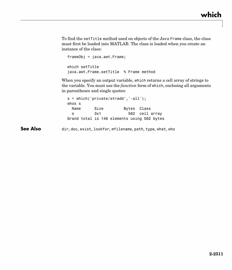
which
2-2511
To find the setTitle method used on objects of the Java Frame class, the class must first be loaded into MATLAB. The class is loaded when you create an instance of the class:
frameObj = java.awt.Frame;
which setTitlejava.awt.Frame.setTitle % Frame method
When you specify an output variable, which returns a cell array of strings to the variable. You must use the function form of which, enclosing all arguments in parentheses and single quotes:
s = which('private/stradd','-all');whos s Name Size Bytes Class s 3x1 562 cell arrayGrand total is 146 elements using 562 bytes
See Also dir, doc, exist, lookfor, mfilename, path, type, what, who

while
2-2512
2whilePurpose Repeat statements an indefinite number of times
Syntax while expressionstatements
end
Description while repeats statements an indefinite number of times. The statements are executed while the real part of expression has all nonzero elements. expression is usually of the form
expression rel_op expression
where rel_op is ==, <, >, <=, >=, or ~=.
The scope of a while statement is always terminated with a matching end.
Arguments expressionexpression is a MATLAB expression, usually consisting of variables or smaller expressions joined by relational operators (e.g., count < limit) or logical functions (e.g., isreal(A)).
Simple expressions can be combined by logical operators (&, |, ~) into compound expressions such as the following. MATLAB evaluates compound expressions from left to right, adhering to operator precedence rules.
(count < limit) & ((height - offset) >= 0)
statementsstatements is one or more MATLAB statements to be executed only while the expression is true or nonzero.
Remarks Nonscalar ExpressionsIf the evaluated expression yields a nonscalar value, then every element of this value must be true or nonzero for the entire expression to be considered true. For example, the statement while (A < B) is true only if each element of matrix A is less than its corresponding element in matrix B. See Example 2, below.

while
2-2513
Partial Evaluation of the Expression ArgumentWithin the context of an if or while expression, MATLAB does not necessarily evaluate all parts of a logical expression. In some cases it is possible, and often advantageous, to determine whether an expression is true or false through only partial evaluation.
For example, if A equals zero in statement 1 below, then the expression evaluates to false, regardless of the value of B. In this case, there is no need to evaluate B and MATLAB does not do so. In statement 2, if A is nonzero, then the expression is true, regardless of B. Again, MATLAB does not evaluate the latter part of the expression.
1) while (A & B) 2) while (A | B)
You can use this property to your advantage to cause MATLAB to evaluate a part of an expression only if a preceding part evaluates to the desired state. Here are some examples.
while (b ~= 0) & (a/b > 18.5)
if exist('myfun.m') & (myfun(x) >= y)
if iscell(A) & all(cellfun('isreal', A))
Examples Example 1 - Simple while StatementThe variable eps is a tolerance used to determine such things as near singularity and rank. Its initial value is the machine epsilon, the distance from 1.0 to the next largest floating-point number on your machine. Its calculation demonstrates while loops.
eps = 1;while (1+eps) > 1
eps = eps/2;endeps = eps*2

while
2-2514
Example 2 - Nonscalar ExpressionGiven matrices A and B,
A = B = 1 0 1 1 2 3 3 4
See Also end, for, break, continue, return, all, any, if, switch
Expression Evaluates As Because
A < B false A(1,1) is not less than B(1,1).
A < (B + 1) true Every element of A is less than that same element of B with 1 added.
A & B false A(1,2) & B(1,2) is false.
B < 5 true Every element of B is less than 5.

whitebg
2-2515
2whitebgPurpose Change axes background color
Syntax whitebgwhitebg(h)whitebg(ColorSpec)whitebg(h,ColorSpec)
Description whitebg complements the colors in the current figure.
whitebg(h) complements colors in all figures specified in the vector h.
whitebg(ColorSpec) and whitebg(h,ColorSpec) change the color of the axes, which are children of the figure, to the color specified by ColorSpec.
Remarks whitebg changes the colors of the figure’s children, with the exception of shaded surfaces. This ensures that all objects are visible against the new background color. whitebg sets the default properties on the root such that all subsequent figures use the new background color.
Examples Set the background color to blue-gray.
whitebg([0 .5 .6])
Set the background color to blue.
whitebg('blue')
See Also ColorSpec
The figure graphics object property InvertHardCopy
“Color Operations” for related functions

who, whos
2-2516
2who, whosPurpose List variables in the workspace
Graphical Interface
As an alternative to whos, use the Workspace browser.
Syntax Each of these syntaxes apply to both who and whos:
whowho(variable_list)who(variable_list, qualifiers)s = who(variable_list, qualifiers)who variable_list qualifiers
Description who lists the variables currently in the workspace.
whos lists the current variables and their sizes and types. It also reports the totals for sizes.
who(variable_list) and whos(variable_list) list only those variables specified in variable_list, where variable_list is a comma-delimited list of quoted strings: 'var1', 'var2', ..., 'varN'. You can use the wildcard character * to display variables that match a pattern. For example, who('A*') finds all variables in the current workspace that start with A.
who(variable_list, qualifiers) and whos(variable_list, qualifiers)list those variables in variable_list that meet all qualifications specified in qualifiers. You can specify any or all of the following qualifiers, and in any order.
Qualifier Syntax Description Example
'global' List variables in the global workspace.
whos('global')

who, whos
2-2517
s = who(variable_list, qualifiers) returns cell array s containing the names of the variables specified in variable_list that meet the conditions specified in qualifiers.
s = whos(variable_list, qualifiers) returns structure s containing the following fields for the variables specified in variable_list that meet the conditions specified in qualifiers:
name variable namesize variable sizebytes number of bytes allocated for the arrayclass class of variable
who variable_list qualifiers and whos variable_list qualifiers are the unquoted forms of the syntax. Both variable_list and qualifiers are space-delimited lists of unquoted strings.
Remarks Information returned by the command whos -file is independent of whether the data in that file is compressed or not. The byte counts returned by this command represent the number of bytes data occupies in the MATLAB workspace, and not in the file the data was saved to. See the function reference for save for more information on data compression.
Examples Show variable names starting with the letter a:
who a*
Show variables stored in MAT-file mydata.mat that start with java and end with Array. Also show their dimensions and class name:
whos -file mydata -regexp \<java.*Array\>
'-file', filename List variables in the specified MAT-file. Use the full path for filename.
whos('-file', 'mydata')
'-regexp', exprlist List variables that match any of the regular expressions in exprlist.
whos('-regexp', '[AB].', '\w\d')
Qualifier Syntax Description Example

who, whos
2-2518
Name Size Bytes Class
javaChrArray 3x1 java.lang.String[][][] javaDblArray 4x1 java.lang.Double[][] javaIntArray 14x1 java.lang.Integer[][]
Get variable names that start with uppercase or lowercase X, are followed by zero or more other characters, and end with at least two digits. Assign the output to cell array xvars:
xvars = who('-regexp', '^[Xx].*\d2,$')xvars = 'X_JohnDavis_5May03' 'Xtest_120' 'xArray5by12' 'x_times_3pt82'
See Also assignin, clear, computer, dir, evalin, exist, inmem, load, save, what, workspace
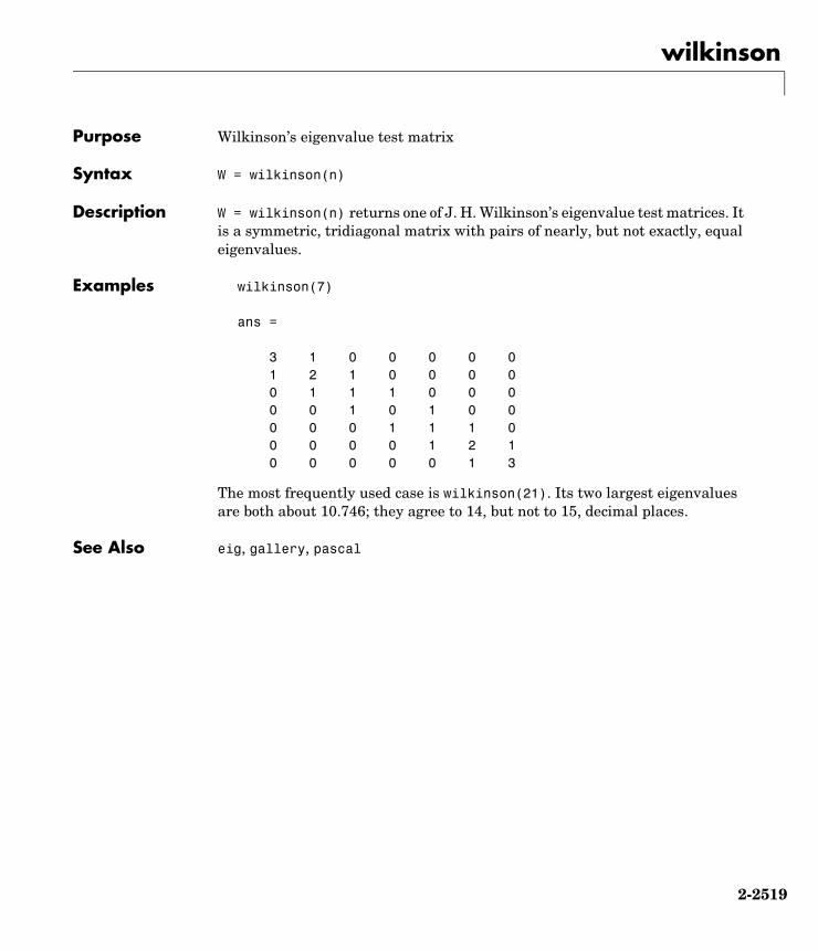
wilkinson
2-2519
2wilkinsonPurpose Wilkinson’s eigenvalue test matrix
Syntax W = wilkinson(n)
Description W = wilkinson(n) returns one of J. H. Wilkinson’s eigenvalue test matrices. It is a symmetric, tridiagonal matrix with pairs of nearly, but not exactly, equal eigenvalues.
Examples wilkinson(7)
ans =
3 1 0 0 0 0 01 2 1 0 0 0 00 1 1 1 0 0 00 0 1 0 1 0 00 0 0 1 1 1 00 0 0 0 1 2 10 0 0 0 0 1 3
The most frequently used case is wilkinson(21). Its two largest eigenvalues are both about 10.746; they agree to 14, but not to 15, decimal places.
See Also eig, gallery, pascal
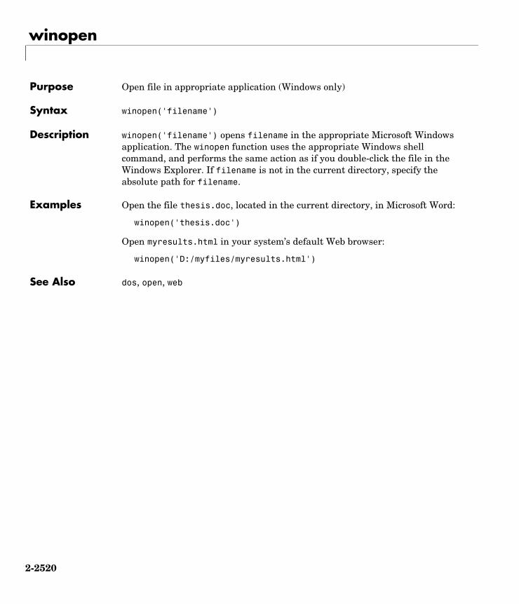
winopen
2-2520
2winopenPurpose Open file in appropriate application (Windows only)
Syntax winopen('filename')
Description winopen('filename') opens filename in the appropriate Microsoft Windows application. The winopen function uses the appropriate Windows shell command, and performs the same action as if you double-click the file in the Windows Explorer. If filename is not in the current directory, specify the absolute path for filename.
Examples Open the file thesis.doc, located in the current directory, in Microsoft Word:
winopen('thesis.doc')
Open myresults.html in your system’s default Web browser:
winopen('D:/myfiles/myresults.html')
See Also dos, open, web

winqueryreg
2-2521
2winqueryreg Purpose Get item from Microsoft Windows registry
Syntax value = winqueryreg('name', 'rootkey', 'subkey')value = winqueryreg('rootkey', 'subkey', 'valname')value = winqueryreg('rootkey', 'subkey')
Description value = winqueryreg('name', 'rootkey', 'subkey') returns the key names in rootkey\subkey in a cell array of strings. The first argument is the literal quoted string, 'name'.
If the value retrieved from the registry is a string, winqueryreg returns a string. If the value is a 32-bit integer, winqueryreg returns the value as an integer of MATLAB type int32.
value = winqueryreg('rootkey', 'subkey', 'valname') returns the value for key valname in rootkey\subkey.
value = winqueryreg('rootkey', 'subkey') returns a value in rootkey\subkey that has no value name property.
Note The literal name argument and the rootkey argument are case-sensitive. The subkey and valname arguments are not.
Remarks This function works only for the following registry value types:
• strings (REG_SZ)
• expanded strings (REG_EXPAND_SZ)
• 32-bit integer (REG_DWORD)
Examples Example 1Get the value of CLSID for the MATLAB sample COM control mwsampctrl.2:
winqueryreg 'HKEY_CLASSES_ROOT' 'mwsamp.mwsampctrl.2\clsid'
ans = 5771A80A-2294-4CAC-A75B-157DCDDD3653

winqueryreg
2-2522
Example 2Get a list in variable mousechar for registry subkey Mouse, which is under subkey Control Panel, which is under root key HKEY_CURRENT_USER.
mousechar = winqueryreg('name', 'HKEY_CURRENT_USER', ... 'control panel\mouse');
For each name in the mousechar list, get its value from the registry and then display the name and its value:
for k=1:length(mousechar) setting = winqueryreg('HKEY_CURRENT_USER', ... 'control panel\mouse', mousechark); str = sprintf('%s = %s', mousechark, num2str(setting)); disp(str) end
ActiveWindowTracking = 0DoubleClickHeight = 4DoubleClickSpeed = 830DoubleClickWidth = 4MouseSpeed = 1MouseThreshold1 = 6MouseThreshold2 = 10SnapToDefaultButton = 0SwapMouseButtons = 0
See Also

wk1finfo
2-2523
2wk1finfoPurpose Determine if file contains Lotus WK1 worksheet
Syntax [extens, type] = wk1finfo('filename')
Description [extens, type] = wk1finfo('filename') returns the string 'WK1' in extens, and 'Lotus 123 Spreadsheet' in type if the file filename contains a readable Lotus worksheet.
Examples This example returns information on spreadsheet file matA.wk1:
[extens, type] = wk1finfo('matA.wk1')
extens = WK1type = Lotus 123 Spreadsheet
See Also wk1read, wk1write, csvread, csvwrite

wk1read
2-2524
2wk1readPurpose Read Lotus123 spreadsheet file (.wk1)
Syntax M = wk1read(filename)M = wk1read(filename,r,c)M = wk1read(filename,r,c,range)
Description M = wk1read(filename) reads a Lotus123 WK1 spreadsheet file into the matrix M.
M = wk1read(filename,r,c) starts reading at the row-column cell offset specified by (r,c). r and c are zero based so that r=0, c=0 specifies the first value in the file.
M = wk1read(filename,r,c,range) reads the range of values specified by the parameter range, where range can be
• A four-element vector specifying the cell range in the format
[upper_left_row upper_left_col lower_right_row lower_right_col]
• A cell range specified as a string, for example, 'A1...C5'
• A named range specified as a string, for example, 'Sales'
Examples Create a 8-by-8 matrix A and export it to Lotus spreadsheet matA.wk1:
A = [1:8; 11:18; 21:28; 31:38; 41:48; 51:58; 61:68; 71:78]A = 1 2 3 4 5 6 7 8 11 12 13 14 15 16 17 18 21 22 23 24 25 26 27 28 31 32 33 34 35 36 37 38 41 42 43 44 45 46 47 48
MATLAB Matrix
Spreadsheet
column
row

wk1read
2-2525
51 52 53 54 55 56 57 58 61 62 63 64 65 66 67 68 71 72 73 74 75 76 77 78
wk1write('matA.wk1', A);
To read in a limited block of the spreadsheet data, specify the upper left row and column of the block using zero-based indexing:
M = wk1read('matA.wk1', 3, 2)M = 33 34 35 36 37 38 43 44 45 46 47 48 53 54 55 56 57 58 63 64 65 66 67 68 73 74 75 76 77 78
To select a more restricted block of data, you can specify both the upper left and lower right corners of the block you want imported. Read in a range of values from row 4, column 3 (defining the upper left corner) to row 6, column 6 (defining the lower right corner). Note that, unlike the second and third arguments, the range argument [4 3 6 6] is one-based:
M = wk1read('matA.wk1', 3, 2, [4 3 6 6])M = 33 34 35 36 43 44 45 46 53 54 55 56
See Also wk1write

wk1write
2-2526
2wk1writePurpose Write a matrix to a Lotus123 WK1 spreadsheet file
Syntax wk1write(filename,M)wk1write(filename,M,r,c)
Description wk1write(filename,M) writes the matrix M into a Lotus123 WK1 spreadsheet file named filename.
wk1write(filename,M,r,c) writes the matrix starting at the spreadsheet location (r,c). r and c are zero based so that r=0, c=0 specifies the first cell in the spreadsheet.
Examples Write a 4-by-5 matrix A to spreadsheet file matA.wk1. Place the matrix with its upper left corner at row 2, column 3 using zero-based indexing:
A = [1:5; 11:15; 21:25; 31:35]A = 1 2 3 4 5 11 12 13 14 15 21 22 23 24 25 31 32 33 34 35
wk1write('matA.wk1', A, 2, 3)
M = wk1read('matA.wk1')M = 0 0 0 0 0 0 0 0 0 0 0 0 0 0 0 0 0 0 0 1 2 3 4 5 0 0 0 11 12 13 14 15 0 0 0 21 22 23 24 25
MATLAB Matrix
Spreadsheet
column
row

wk1write
2-2527
0 0 0 31 32 33 34 35
See Also wk1read, dlmwrite, dlmread, csvwrite, csvread

workspace
2-2528
2workspacePurpose Display the Workspace browser, a tool for managing the workspace
Graphical Interface
As an alternative to the workspace function, select Workspace from the Desktop menu in the MATLAB desktop.
Syntax workspace
Description workspace displays the Workspace browser, a graphical user interface that allows you to view and manage the contents of the MATLAB workspace. It provides a graphical representation of the whos display, and allows you to perform the equivalent of the clear, load, open, and save functions.
To see and edit a graphical representation of a variable, double-click the variable in the Workspace browser. The variable is displayed in the Array Editor, where you can edit it.
See Also who

xlabel, ylabel, zlabel
2-2529
2xlabel, ylabel, zlabelPurpose Label the x-, y-, and z-axis
Syntax xlabel('string')xlabel(fname)xlabel(...,'PropertyName',PropertyValue,...)xlabel(axes_handle,...)h = xlabel(...)
ylabel(...)ylabel(axes_handle,...)h = ylabel(...)
zlabel(...)zlabel(axes_handle,...)h = zlabel(...)
Description Each axes graphics object can have one label for the x-, y-, and z-axis. The label appears beneath its respective axis in a two-dimensional plot and to the side or beneath the axis in a three-dimensional plot.
xlabel('string') labels the x-axis of the current axes.
xlabel(fname) evaluates the function fname, which must return a string, then displays the string beside the x-axis.
xlabel(...,'PropertyName',PropertyValue,...) specifies property name and property value pairs for the text graphics object created by xlabel.
xlabel(axes_handle,...), ylabel(axes_handle,...), and zlabel(axes_handle,...) plot into the axes with handle axes_handle instead of the current axes (gca).
h = xlabel(...), h = ylabel(...), and h = zlabel(...) return the handle to the text object used as the label.
ylabel(...) and zlabel(...) label the y-axis and z-axis, respectively, of the current axes.

xlabel, ylabel, zlabel
2-2530
Remarks Reissuing an xlabel, ylabel, or zlabel command causes the new label to replace the old label.
For three-dimensional graphics, MATLAB puts the label in the front or side, so that it is never hidden by the plot.
Examples Create a multiline label for the x-axis using a multiline cell array.
xlabel('first line';'second line')
See Also text, title
“Annotating Plots” for related functions
Adding Axis Labels to Graphs for more information about labeling axes

xlim, ylim, zlim
2-2531
2xlim, ylim, zlimPurpose Set or query axis limits
Syntax Note that the syntax for each of these three functions is the same; only the xlim function is used for simplicity. Each operates on the respective x-, y-, or z-axis.
xlimxlim([xmin xmax])xlim('mode')xlim('auto')xlim('manual')xlim(axes_handle,...)
Description xlim with no arguments returns the respective limits of the current axes.
xlim([xmin xmax]) sets the axis limits in the current axes to the specified values.
xlim('mode') returns the current value of the axis limits mode, which can be either auto (the default) or manual.
xlim('auto') sets the axis limit mode to auto.
xlim('manual') sets the respective axis limit mode to manual.
xlim(axes_handle,...) performs the set or query on the axes identified by the first argument, axes_handle. When you do not specify an axes handle, these functions operate on the current axes.
Remarks xlim, ylim, and zlim set or query values of the axes object XLim, YLim, ZLim, and XLimMode, YLimMode, ZLimMode properties.
When the axis limit modes are auto (the default), MATLAB uses limits that span the range of the data being displayed and are round numbers. Setting a value for any of the limits also sets the corresponding mode to manual. Note that high-level plotting functions like plot and surf reset both the modes and the limits. If you set the limits on an existing graph and want to maintain these limits while adding more graphs, use the hold command.

xlim, ylim, zlim
2-2532
Examples This example illustrates how to set the x- and y-axis limits to match the actual range of the data, rather than the rounded values of [-2 3] for the x-axis and [-2 4] for the y-axis originally selected by MATLAB.
[x,y] = meshgrid([−1.75:.2:3.25]);z = x.*exp(−x.^2−y.^2);surf(x,y,z)xlim([−1.75 3.25])ylim([−1.75 3.25])
See Also axis
The axes properties XLim, YLim, ZLim
“Setting the Aspect Ratio and Axis Limits” for related functions
Understanding Axes Aspect Ratio for more information on how axis limits affect the axes
−10
12
3
−1
0
1
2
3
−0.5
0
0.5

xlsfinfo
2-2533
2xlsfinfoPurpose Determine if file contains Microsoft Excel (.xls) spreadsheet
Syntax type = xlsfinfo('filename')[type, sheets] = xlsfinfo('filename')xlsfinfo filename
Description type = xlsfinfo('filename') returns the string 'Microsoft Excel Spreadsheet' in the type output if the file specified by filename can be read by the MATLAB function xlsread. Otherwise, type is the empty string.
[type, sheets] = xlsfinfo('filename') returns in the sheets output a cell array of strings containing the names of each spreadsheet in the file.
xlsfinfo filename is the command format for xlsfinfo.
Examples When filename is an Excel spreadsheet,
[type, sheets] = xlsfinfo('myaccount.xls')
type = Microsoft Excel Spreadsheet
sheets = 'Sheet1' 'Income' 'Expenses'
See Also xlsread, xlswrite

xlsread
2-2534
2xlsreadPurpose Read Microsoft Excel spreadsheet file (.xls)
Syntax N = xlsread('filename')N = xlsread('filename', -1)N = xlsread('filename', sheet)N = xlsread('filename', 'range')N = xlsread('filename', sheet, 'range')N = xlsread('filename', sheet, 'range', 'basic')[N, T] = xlsread('filename', ...)[N, T, rawdata] = xlsread('filename', ...)xlsread filename sheet range basic
Description N = xlsread('filename') returns numeric data in double array N from the first sheet in the Microsoft Excel spreadsheet file named filename. The xlsread ignores leading rows or columns of text. However, if a cell not in a leading row or column is empty or contains text, xlsread puts a NaN in its place in the return array, N.
N = xlsread('filename', -1) opens the file filename in an Excel window, enabling you to interactively select the worksheet to be read and the range of data on that worksheet to import. To import an entire worksheet, first select the sheet in the Excel window and then click the OK button in the Data Selection Dialog box. To import a certain range of data from the sheet, select the worksheet in the Excel window, drag and drop the mouse over the desired range, and then click OK. (See “COM Server Requirements” below.)
N = xlsread('filename', sheet) reads the specified worksheet, where sheet is either a positive, double scalar value or a quoted string containing the sheet name. To determine the names of the sheets in a spreadsheet file, use xlsfinfo.
N = xlsread('filename', 'range') reads data from a specific rectangular region of the default worksheet (Sheet1). Specify range using the syntax 'C1:C2', where C1 and C2 are two opposing corners that define the region to be read. For example, 'D2:H4' represents the 3-by-5 rectangular region between the two corners D2 and H4 on the worksheet. The range input is not case sensitive and uses Excel A1 notation. (See help in Excel for more information on this notation.) (Also, see “COM Server Requirements” below.)

xlsread
2-2535
N = xlsread('filename', sheet, 'range') reads data from a specific rectangular region (range) of the worksheet specified by sheet. See the previous two syntax formats for further explanation of the sheet and range inputs. (See “COM Server Requirements,” below.)
N = xlsread('filename', sheet, 'range', 'basic') imports data from the spreadsheet in basic import mode. sheet must be a quoted string and is case sensitive. range is ignored and can be set to the empty string ('').
[N, T]= xlsread('filename', ...) returns numeric data in array N and text data in cell array T. All cells in T that correspond to numeric data contain the empty string.
If T includes data that was previously written to the file using xlswrite, and the range specified for that xlswrite operation caused undefined data ('#N/A') to be written to the worksheet, then cells containing that undefined data are represented in the T output as 'ActiveX VT_ERROR: '.
[N, T, rawdata] = xlsread('filename', ...) returns numeric and text data in N and T, and unprocessed cell content in cell array rawdata, which contains both numeric and text data. (See “COM Server Requirements” below.)
xlsread filename sheet range basic is the command format for xlsread, showing its usage with all input arguments specified. When using this format, you must specify sheet as a string, (for example, Income or Sheet4) and not a numeric index. If the sheet name contains space characters, then quotation marks are required around the string, (for example, 'Income 2002').
Remarks COM Server RequirementsThe following four syntax formats are supported only on computer systems capable of starting Excel as a COM server from MATLAB.
N = xlsread('filename', -1)N = xlsread('filename', 'range')N = xlsread('filename', sheet, 'range')[N, T, rawdata] = xlsread('filename', ...)

xlsread
2-2536
Examples Example 1— Reading Numeric Data The Microsoft Excel spreadsheet file testdata1.xls contains this data:
1 62 73 84 95 10
To read this data into MATLAB, use this command:
A = xlsread('testdata1.xls')A =
1 62 73 84 95 10
Example 2 — Handling Text DataThe Microsoft Excel spreadsheet file testdata2.xls contains a mix of numeric and text data:
1 62 73 84 95 text
xlsread puts a NaN in place of the text data in the result:
A = xlsread('testdata2.xls')A =
1 62 73 84 95 NaN
Example 3 — Selecting a Range of DataTo import only rows 4 and 5 from worksheet 1, specify the range as 'A4:B5':

xlsread
2-2537
A = xlsread('testdata2.xls', 1, 'A4:B5')
A =4 95 NaN
Example 4 — Handling Files with Row or Column HeadersA Microsoft Excel spreadsheet labeled Temperatures in file tempdata.xls contains two columns of numeric data with text headers for each column:
Time Temp12 9813 9914 97
If you want to import only the numeric data, use xlsread with a single return argument. Specify the filename and sheet name as inputs.
xlsread ignores any leading row or column of text in the numeric result.
ndata = xlsread('tempdata.xls', 'Temperatures')
ndata = 12 98 13 99 14 97
To import both the numeric data and the text data, specify two return values for xlsread:
[ndata, headertext] = xlsread('tempdata.xls', 'Temperatures')
ndata = 12 98 13 99 14 97
headertext = 'Time' 'Temp'
See Also xlswrite, xlsfinfo, wk1read, textread
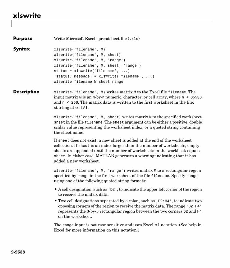
xlswrite
2-2538
2xlswritePurpose Write Microsoft Excel spreadsheet file (.xls)
Syntax xlswrite('filename', M)xlswrite('filename', M, sheet)xlswrite('filename', M, 'range')xlswrite('filename', M, sheet, 'range')status = xlswrite('filename', ...)[status, message] = xlswrite('filename', ...)xlswrite filename M sheet range
Description xlswrite('filename', M) writes matrix M to the Excel file filename. The input matrix M is an m-by-n numeric, character, or cell array, where m < 65536 and n < 256. The matrix data is written to the first worksheet in the file, starting at cell A1.
xlswrite('filename', M, sheet) writes matrix M to the specified worksheet sheet in the file filename. The sheet argument can be either a positive, double scalar value representing the worksheet index, or a quoted string containing the sheet name.
If sheet does not exist, a new sheet is added at the end of the worksheet collection. If sheet is an index larger than the number of worksheets, empty sheets are appended until the number of worksheets in the workbook equals sheet. In either case, MATLAB generates a warning indicating that it has added a new worksheet.
xlswrite('filename', M, 'range') writes matrix M to a rectangular region specified by range in the first worksheet of the file filename. Specify range using one of the following quoted string formats:
• A cell designation, such as 'D2', to indicate the upper left corner of the region to receive the matrix data.
• Two cell designations separated by a colon, such as 'D2:H4', to indicate two opposing corners of the region to receive the matrix data. The range 'D2:H4' represents the 3-by-5 rectangular region between the two corners D2 and H4 on the worksheet.
The range input is not case sensitive and uses Excel A1 notation. (See help in Excel for more information on this notation.)

xlswrite
2-2539
The size defined by range should fit the size of M or contain only the first cell, (e.g., 'A2'). If range is larger than the size of M, Excel fills the remainder of the region with #N/A. If range is smaller than the size of M, only the submatrix that fits into range is written to the file specified by filename.
xlswrite('filename', M, sheet, 'range') writes matrix M to a rectangular region specified by range in worksheet sheet of the file filename. See the previous two syntax formats for further explanation of the sheet and range inputs.
status = xlswrite('filename', ...) returns the completion status of the write operation in status. If the write completed successfully, status is equal to 1 (or true). Otherwise, status is 0 (or false). Unless you specify an output for xlswrite, no status is displayed in the Command Window.
[status, message] = xlswrite('filename', ...) returns any warning or error message generated by the write operation in the MATLAB structure message. The message structure has two fields:
• message — String containing the text of the warning or error message
• identifier — String containing the message identifier for the warning or error
xlswrite filename M sheet range is the command format for xlswrite, showing its usage with all input arguments specified. When using this format, you must specify sheet as a string (for example, Income or Sheet4). If the sheet name contains space characters, then quotation marks are required around the string (for example, 'Income 2002').
Examples Example 1 — Writing Numeric Data to the Default WorksheetWrite a 7-element vector to Microsoft Excel file testdata.xls. By default, the data is written to cells A1 through G1 in the first worksheet in the file:
xlswrite('testdata', [12.7 5.02 -98 63.9 0 -.2 56])
Example 2 — Writing Mixed Data to a Specific WorksheetThis example writes the following mixed text and numeric data to the file tempdata.xls:
d = 'Time', 'Temp'; 12 98; 13 99; 14 97;

xlswrite
2-2540
Call xlswrite, specifying the worksheet labeled Temperatures, and the region within the worksheet to write the data to. The 4-by-2 matrix will be written to the rectangular region that starts at cell E1 in its upper left corner:
s = xlswrite('tempdata.xls', d, 'Temperatures', 'E1')s = 1
The output status s shows that the write operation succeeded. The data appears as shown here in the output file:
Time Temp 12 98 13 99 14 97
Example 3 — Appending a New Worksheet to the FileNow write the same data to a worksheet that doesn’t yet exist in tempdata.xls. In this case, MATLAB appends a new sheet to the workbook, calling it by the name you supplied in the sheets input argument, 'NewTemp'. MATLAB displays a warning indicating that it has added a new worksheet to the file:
xlswrite('tempdata.xls', d, 'NewTemp', 'E1')Warning: Added specified worksheet.
If you don’t want to see these warnings, you can turn them off using the command indicated in the message above:
warning off MATLAB:xlswrite:AddSheet
Now try the command again, this time creating another new worksheet, NewTemp2. Although the message is not displayed this time, you can still retrieve it and its identifier from the second output argument, m:
[stat mmsg] = xlswrite('tempdata.xls', d, 'NewTemp2', 'E1');
msgmsg = message: 'Added specified worksheet.' identifier: 'MATLAB:xlswrite:AddSheet'
See Also xlsread, xlsfinfo, wk1read, textread

xmlread
2-2541
2xmlreadPurpose Parse XML document and return Document Object Model node
Syntax DOMnode = xmlread(filename)
Description DOMnode = xmlread(filename) reads a URL or filename and returns a Document Object Model node representing the parsed document.
Remarks Find out more about the Document Object Model at the World Wide Web Consortium (W3C) Web site, http://www.w3.org/DOM/. For specific information on using Java DOM objects, visit the Sun Web site, http://www.java.sun.com/xml/docs/api.
See Also xmlwrite, xslt

xmlwrite
2-2542
2xmlwritePurpose Serialize XML Document Object Model node
Syntax xmlwrite(filename, DOMnode)str = xmlwrite(DOMnode)
Description xmlwrite(filename, DOMnode) serializes the Document Object Model node DOMnode to the file specified by filename.
str = xmlwrite(DOMnode) serializes the Document Object Model node DOMnode and returns the node tree as a string, s.
Remarks Find out more about the Document Object Model at the World Wide Web Consortium (W3C) Web site, http://www.w3.org/DOM/. For specific information on using Java DOM objects, visit the Sun Web site, http://www.java.sun.com/xml/docs/api.
Example % Create a sample XML document.docNode = com.mathworks.xml.XMLUtils.createDocument... ('root_element')docRootNode = docNode.getDocumentElement;for i=1:20 thisElement = docNode.createElement('child_node'); thisElement.appendChild... (docNode.createTextNode(sprintf('%i',i))); docRootNode.appendChild(thisElement);enddocNode.appendChild(docNode.createComment('this is a comment'));
% Save the sample XML document.xmlFileName = [tempname,'.xml'];xmlwrite(xmlFileName,docNode);edit(xmlFileName);
See Also xmlread, xslt

xor
2-2543
2xorPurpose Exclusive or
Syntax C = xor(A, B)
Description C = xor(A, B) performs an exclusive OR operation on the corresponding elements of arrays A and B. The resulting element C(i,j,...) is logical true (1) if A(i,j,...) or B(i,j,...), but not both, is nonzero.
Examples Given A = [0 0 pi eps] and B = [0 -2.4 0 1], then
C = xor(A,B)C = 0 1 1 0
To see where either A or B has a nonzero element and the other matrix does not,
spy(xor(A,B))
See Also all, any, find, Elementwise Logical Operators, Short-Circuit Logical Operators
A B C
Zero Zero 0
Zero Nonzero 1
Nonzero Zero 1
Nonzero Nonzero 0
xslt
2-2544
2xsltPurpose Transform XML document using XSLT engine
Syntax result = xslt(source, style, dest)[result,style] = xslt(...)xslt(...,'-web')
Description result = xslt(source, style, dest) transforms an XML document using a stylesheet and returns the resulting document's URL. The function uses these inputs, the first of which is required:
• source is the filename or URL of the source XML file. source can also specify a DOM node.
• style is the filename or URL of an XSL stylesheet.
• dest is the filename or URL of the desired output document. If dest is absent or empty, the function uses a temporary filename. If dest is '-tostring', the function returns the output document as a MATLAB string.
[result,style] = xslt(...) returns a processed stylesheet appropriate for passing to subsequent XSLT calls as style. This prevents costly repeated processing of the stylesheet.
xslt(...,'-web') displays the resulting document in the Help Browser.
Remarks Find out more about XSL stylesheets and how to write them at the World Wide Web Consortium (W3C) web site, http://www.w3.org/Style/XSL/.
Example This example converts the file info.xml using the stylesheet info.xsl, writing the output to the file info.html. It launches the resulting HTML file in the Help Browser. MATLAB has several info.xml files that are used by the Start menu.
xslt info.xml info.xsl info.html -web
See Also xmlread, xmlwrite

zeros
2-2545
2zerosPurpose Create an array of all zeros
Syntax B = zeros(n)B = zeros(m,n)B = zeros([m n])B = zeros(d1,d2,d3...)B = zeros([d1 d2 d3...])B = zeros(size(A))zeros(m, n,...,classname)zeros([m,n,...],classname)
Description B = zeros(n) returns an n-by-n matrix of zeros. An error message appears if n is not a scalar.
B = zeros(m,n) or B = zeros([m n]) returns an m-by-n matrix of zeros.
B = zeros(d1,d2,d3...) or B = zeros([d1 d2 d3...]) returns an array of zeros with dimensions d1-by-d2-by-d3-by-... .
B = zeros(size(A)) returns an array the same size as A consisting of all zeros.
zeros(m, n,...,classname) or zeros([m,n,...],classname) is an m-by-n-by-... array of zeros of data type classname. classname is a string specifying the data type of the output. classname can have the following values: 'double', 'single', 'int8', 'uint8', 'int16', 'uint16', 'int32', or 'uint32'.
Example x = zeros(2,3,'int8');
Remarks The MATLAB language does not have a dimension statement; MATLAB automatically allocates storage for matrices. Nevertheless, for large matrices, MATLAB programs may execute faster if the zeros function is used to set aside storage for a matrix whose elements are to be generated one at a time, or a row or column at a time. For example
x = zeros(1,n);for i = 1:n, x(i) = i; end

zeros
2-2546
See Also eye, ones, rand, randn

zip
2-2547
2zipPurpose Create compressed version of files in zip format
Syntax zip('zipfilename','files')zip('zipfilename','directory')zip(...,'rootdirectory')
Description zip('zipfilename','files') creates a zip file named zipfilename from the file named files. For multiple files, make files a cell array of strings. Paths for zipfilename and files are relative to the current directory. Zip files are often used for archiving or for minimizing file transmission time.
zip('zipfilename','directory') creates a zip file named zipfilename consisting of the specified directory and all the files in it. The paths for zipfilename and directory are relative to the current directory.
zip('zipfilename','source','rootdirectory') allows the path specified for source to be relative to 'rootdirectory' rather than to the current directory. Note that source cannot be an absolute path.
Examples Zipping a FileCreate a zip file of the file guide.viewlet, which is in the demos directory of MATLAB. It saves the zip file in d:/mymfiles/viewlet.zip.
zip('d:/mymfiles/viewlet.zip','$matlabroot/demos/guide.viewlet')
Zip the files guide.viewlet and import.viewlet and save the zip file in viewlets.zip. The source files and zipped file are in the current directory.
zip('viewlets.zip','guide.viewlet','import.viewlet')
Zipping a DirectoryZip the directory D:/mymfiles and its contents to the zip file mymfiles in the directory one level up from the current directory.
zip('../mymfiles','D:/mymfiles')
Zip the files thesis.doc and defense.ppt, which are located in d:/PhD, to the zip file thesis.zip in the current directory.
zip('thesis.zip','thesis.doc','defense.ppt','d:/PhD')

zip
2-2548
See Also unzip

zoom
2-2549
2zoomPurpose Zoom in and out on a 2-D plot
Syntax zoom onzoom offzoom outzoom resetzoomzoom xonzoom yonzoom(factor)zoom(fig, option)
Description zoom on turns on interactive zooming. When interactive zooming is enabled in a figure, pressing a mouse button while your cursor is within an axes zooms into the point or out from the point beneath the mouse. Zooming changes the axes limits.
• For a single-button mouse, zoom in by pressing the mouse button and zoom out by simultaneously pressing Shift and the mouse button.
• For a two- or three-button mouse, zoom in by pressing the left mouse button and zoom out by pressing the right mouse button.
Clicking and dragging over an axes when interactive zooming is enabled draws a rubberband box. When the mouse button is released, the axes zoom in to the region enclosed by the rubberband box.
Double-clicking over an axes returns the axes to its initial zoom setting.
zoom off turns interactive zooming off.
zoom out returns the plot to its initial zoom setting.
zoom reset remembers the current zoom setting as the initial zoom setting. Later calls to zoom out, or double-clicks when interactive zoom mode is enabled, will return to this zoom level.
zoom toggles the interactive zoom status.
zoom xon and zoom yon set zoom on for the x- and y-axis, respectively.

zoom
2-2550
zoom(factor) zooms in or out by the specified zoom factor, without affecting the interactive zoom mode. Values greater than 1 zoom in by that amount, while numbers greater than 0 and less than 1 zoom out by 1/factor.
zoom(fig, option) Any of the above options can be specified on a figure other than the current figure using this syntax.
Remarks zoom changes the axes limits by a factor of two (in or out) each time you press the mouse button while the cursor is within an axes. You can also click and drag the mouse to define a zoom area, or double-click to return to the initial zoom level.
See Also linkaxes, pan
“Object Manipulation” for related functions

Index-1
Index
Numerics1-norm 2-1810
AAccelerator
Uimenu property 2-2370activelegend 2-1692allocation of storage (automatic) 2-2545AlphaData
surface property 2-2156surfaceplot property 2-2171
AlphaDataMapping
patch property 2-1615surface property 2-2156surfaceplot property 2-2171
AmbientStrength
Patch property 2-1615Surface property 2-2157surfaceplot property 2-2172
annotating plots 2-1693archiving files 2-2547arguments, M-file
passing variable numbers of 2-2455array
product of elements 2-1741of random numbers 2-1799, 2-1801removing first n singleton dimensions of
2-1953removing singleton dimensions of 2-2022reshaping 2-1858shifting dimensions of 2-1953size of 2-1964sorting elements of 2-1974structure 2-1875, 2-1946sum of elements 2-2138swapping dimensions of 2-1672
of all zeros 2-2545arrays
editing 2-2528ASCII data
converting sparse matrix after loading from 2-1984
saving to disk 2-1899aspect ratio of axes 2-1642AutoScale
quivergroup property 2-1783AutoScaleFactor
quivergroup property 2-1783axes
setting and querying limits 2-2531setting and querying plot box aspect ratio
2-1642axes
editing 2-1693azimuth (spherical coordinates) 2-1992azimuth of viewpoint 2-2468
BBackFaceLighting
Surface property 2-2157surfaceplot property 2-2172
BackFaceLightingpatch property 2-1616BackGroundColor
Uicontrol property 2-2339BackgroundColor
Text property 2-2230badly conditioned 2-1810BaseLine
stem property 2-2053BaseValue
stem property 2-2053

Index
Index-2
BeingDeleted
group property 2-2231quivergroup property 2-1783rectangle property 2-1824scatter property 2-1913stairseries property 2-2029stem property 2-2053surface property 2-2157surfaceplot property 2-2172transform property 2-1616Uipushtool property 2-2402Uitoggletool property 2-2424Uitoolbar property 2-2435
binary datasaving to disk 2-1899
bold fontTeX characters 2-2246
bubble plot (scatter function) 2-1909Buckminster Fuller 2-2209BusyAction
patch property 2-1616quivergroup property 2-1783rectangle property 2-1824Root property 2-1878scatter property 2-1913stairseries property 2-2029stem property 2-2053Surface property 2-2158surfaceplot property 2-2173Text property 2-2231Uicontextmenu property 2-2324Uicontrol property 2-2339Uimenu property 2-2371Uipushtool property 2-2402Uitoggletool property 2-2424Uitoolbar property 2-2435
ButtonDownFcn
patch property 2-1617quivergroup property 2-1784rectangle property 2-1825Root property 2-1878scatter property 2-1914stairseries property 2-2030stem property 2-2054Surface property 2-2158surfaceplot property 2-2173Text property 2-2232Uicontextmenu property 2-2324Uicontrol property 2-2340
Ccaching
MATLAB directory 2-1634CallBack
Uicontextmenu property 2-2324Uicontrol property 2-2340Uimenu property 2-2371
CallbackObject, Root property 2-1878CaptureMatrix, Root property 2-1878CaptureRect, Root property 2-1878Cartesian coordinates 2-1702, 2-1992case
in switch statement (defined) 2-2198lower to upper 2-2450
Cayley-Hamilton theorem 2-1718CData
scatter property 2-1914Surface property 2-2158surfaceplot property 2-2173Uicontrol property 2-2341Uipushtool property 2-2403Uitoggletool property 2-2425
CDataMapping

Index
Index-3
patch property 2-1619Surface property 2-2159surfaceplot property 2-2174
CDataMode
surfaceplot property 2-2174CDatapatch property 2-1617CDataSource
scatter property 2-1914surfaceplot property 2-2174
charactersconversion, in format specification string
2-2011escape, in format specification string 2-2012
check boxes 2-2330Checked, Uimenu property 2-2371checkerboard pattern (example) 2-1856child functions 2-1742Children
patch property 2-1620quivergroup property 2-1784rectangle property 2-1825Root property 2-1878scatter property 2-1915stairseries property 2-2030stem property 2-2054Surface property 2-2159surfaceplot property 2-2175Text property 2-2232Uicontextmenu property 2-2324Uicontrol property 2-2341Uimenu property 2-2372Uitoolbar property 2-2436
Cholesky factorizationlower triangular factor 2-1602minimum degree ordering and (sparse) 2-2207
ClickedCallback
Uipushtool property 2-2403
Uitoggletool property 2-2425Clipping
quivergroup property 2-1784rectangle property 2-1825Root property 2-1878, 2-1879scatter property 2-1915stairseries property 2-2030stem property 2-2055Surface property 2-2159surfaceplot property 2-2175Text property 2-2232Uicontextmenu property 2-2324Uicontrol property 2-2341
Clippingpatch property 2-1620closest triangle search 2-2300closing
MATLAB 2-1777Color
quivergroup property 2-1784stairseries property 2-2030stem property 2-2055Text property 2-2232
colormapsconverting from RGB to HSV 2-1866plotting RGB components 2-1867
commandssystem 2-2212UNIX 2-2444
complexnumbers, sorting 2-1974, 2-1977sine 2-1959unitary matrix 2-1759
complex Schur form 2-1925compress files 2-2547condition number of matrix 2-1810context menu 2-2320continued fraction expansion 2-1805

Index
Index-4
conversioncylindrical to Cartesian 2-1702full to sparse 2-1981lowercase to uppercase 2-2450partial fraction expansion to pole-residue
2-1860polar to Cartesian 2-1702pole-residue to partial fraction expansion
2-1860real to complex Schur form 2-1897spherical to Cartesian 2-1992string to numeric array 2-2070
conversion characters in format specification string 2-2011
coordinate system and viewpoint 2-2468coordinates
Cartesian 2-1702, 2-1992cylindrical 2-1702polar 2-1702spherical 2-1992
CreateFcn
patch property 2-1620quivergroup property 2-1785rectangle property 2-1825Root property 2-1879scatter property 2-1915stairseries property 2-2030stemseries property 2-2055Surface property 2-2159surfaceplot property 2-2175Text property 2-2232Uicontextmenu property 2-2324Uicontrol property 2-2341Uimenu property 2-2372Uipushtool property 2-2403Uitoggletool property 2-2425Uitoolbar property 2-2436
cubic interpolation 2-1651current directory 2-1754CurrentFigure, Root property 2-1879Curvature, rectangle property 2-1826curve fitting (polynomial) 2-1711Cuthill-McKee ordering, reverse 2-2207, 2-2209cylindrical coordinates 2-1702
Ddata
ASCII, saving to disk 2-1899binary, saving to disk 2-1899computing 2-D stream lines 2-2076computing 3-D stream lines 2-2078formatting 2-2010reading from files 2-2249reducing number of elements in 2-1838smoothing 3-D 2-1972writing to strings 2-2010
data, ASCIIconverting sparse matrix after loading from
2-1984debugging
M-files 2-1742decomposition
“economy-size” 2-1759, 2-2193orthogonal-triangular (QR) 2-1759Schur 2-1925singular value 2-1804, 2-2193
definite integral 2-1770DeleteFcn
quivergroup property 2-1785Root property 2-1879scatter property 2-1915stairseries property 2-2031stem property 2-2055

Index
Index-5
Surface property 2-2160surfaceplot property 2-2175Text property 2-2233, 2-2234Uicontextmenu property 2-2325, 2-2342Uimenu property 2-2373Uipushtool property 2-2404Uitoggletool property 2-2426Uitoolbar property 2-2437
DeleteFcn, rectangle property 2-1826DeleteFcnpatch property 2-1620dependence, linear 2-2135dependent functions 2-1742derivative
polynomial 2-1708detecting
positive, negative, and zero array elements 2-1958
diagonalk-th (illustration) 2-2290sparse 2-1986
dialog boxprint 2-1739question 2-1776warning 2-2486
Diary, Root property 2-1879DiaryFile, Root property 2-1879differences
between sets 2-1944, 2-1945differential equation solvers
ODE boundary value problemsextracting properties of 2-2288, 2-2289
parabolic-elliptic PDE problems 2-1657DiffuseStrength
Surface property 2-2160surfaceplot property 2-2176
DiffuseStrengthpatch property 2-1621digamma function 2-1750
dimension statement (lack of in MATLAB) 2-2545dimensions
size of 2-1964direct term of a partial fraction expansion 2-1860directories
listing MATLAB files in 2-2506MATLAB
caching 2-1634removing 2-1871removing from search path 2-1876
directorytemporary system 2-2216
directory, current 2-1754discontinuities, eliminating (in arrays of phase
angles) 2-2447DisplayName
quivergroup property 2-1785scatter property 2-1916stairseries property 2-2031stem property 2-2056
divisionremainder after 2-1854
EEcho, Root property 2-1879EdgeAlpha
patch property 2-1621surface property 2-2160surfaceplot property 2-2176
EdgeColor
patch property 2-1621Surface property 2-2161surfaceplot property 2-2176Text property 2-2233
EdgeColor, rectangle property 2-1826EdgeLighting

Index
Index-6
patch property 2-1622Surface property 2-2161surfaceplot property 2-2177
editable text 2-2330eigenvalue
modern approach to computation of 2-1706problem 2-1709problem, generalized 2-1709problem, polynomial 2-1709Wilkinson test matrix and 2-2519
eigenvectormatrix, generalized 2-1798
elevation (spherical coordinates) 2-1992elevation of viewpoint 2-2468Enable
Uicontrol property 2-2342Uimenu property 2-2374Uipushtool property 2-2404Uitogglehtool property 2-2426
EraseMode
quivergroup property 2-1786rectangle property 2-1826scatter property 2-1916stairseries property 2-2031stem property 2-2056Surface property 2-2162surfaceplot property 2-2177Text property 2-2234
EraseModepatch property 2-1622error messages
Out of memory 2-1596ErrorMessage, Root property 2-1880ErrorType, Root property 2-1880escape characters in format specification string
2-2012examples
reducing number of patch faces 2-1835
reducing volume data 2-1838subsampling volume data 2-2141
Excel spreadsheetsloading 2-2534
executing statements repeatedly 2-2512execution
improving speed of by setting aside storage 2-2545
pausing M-file 2-1641time for M-files 2-1742
extension, filename.mat 2-1899
Extent
Text property 2-2235Uicontrol property 2-2343
FFaceAlphapatch property 2-1623FaceAlphasurface property 2-2163FaceAlphasurfaceplot property 2-2178FaceColor
Surface property 2-2163surfaceplot property 2-2179
FaceColor, rectangle property 2-1827FaceColorpatch property 2-1624FaceLighting
Surface property 2-2163surfaceplot property 2-2179
FaceLightingpatch property 2-1624faces, reducing number in patches 2-1834Faces,patch property 2-1624FaceVertexAlphaData, patch property 2-1625FaceVertexCData,patch property 2-1626factorization
QZ 2-1710, 2-1798See also decomposition

Index
Index-7
factorization, Choleskyminimum degree ordering and (sparse) 2-2207
Figureredrawing 2-1840
figuresannotating 2-1693saving 2-1904
filenametemporary 2-2217
filename extension.mat 2-1899
filescompressing 2-2547Excel spreadsheets
loading 2-2534fig 2-1904figure, saving 2-1904listing
in directory 2-2506locating 2-2509mdl 2-1904model, saving 2-1904opening
in Web browser 2-2500opening in Windows applications 2-2520pathname for 2-2509reading
data from 2-2249sound
reading 2-2497writing 2-2499
.wav
reading 2-2497writing 2-2499
WK1loading 2-2524writing to 2-2526
findingsign of array elements 2-1958
finish.m 2-1777fixed-width font
text 2-2236uicontrols 2-2344
FixedWidthFontName, Root property 2-1880floating-point arithmetic, IEEE
smallest postive number 2-1814flow control
return 2-1865switch 2-2198while 2-2512
fontfixed-width, text 2-2236fixed-width, uicontrols 2-2344
FontAngle
Text property 2-2235Uicontrol property 2-2344
FontName
Text property 2-2235Uicontrol property 2-2344
fontsbold 2-2236italic 2-2235specifying size 2-2236TeX characters
bold 2-2246italics 2-2246specifying family 2-2246specifying size 2-2246
units 2-2236FontSize
Text property 2-2236Uicontrol property 2-2344
FontUnits
Text property 2-2236

Index
Index-8
Uicontrol property 2-2344FontWeight
Text property 2-2236Uicontrol property 2-2345
ForegroundColor
Uicontrol property 2-2345Uimenu property 2-2374
Format 2-1880format
specification string, matching file data to 2-2024
FormatSpacing, Root property 2-1881formatting data 2-2010fraction, continued 2-1805fragmented memory 2-1596functions
locating 2-2509pathname for 2-2509that work down the first non-singleton
dimension 2-1953
Ggamma function
logarithmic derivative 2-1750Gaussian elimination
Gauss Jordan elimination with partial pivoting 2-1895
generalized eigenvalue problem 2-1709geodesic dome 2-2209graphics objects
Patch 2-1603resetting properties 2-1857Root 2-1877setting properties 2-1938Surface 2-2152Text 2-2222
uicontextmenu 2-2320Uicontrol 2-2329Uimenu 2-2366
graphsediting 2-1693
Greek letters and mathematical symbols 2-2244GUIs, printing 2-1734
HHadamard matrix
subspaces of 2-2135HandleVisibility
patch property 2-1627quivergroup property 2-1787rectangle property 2-1827Root property 2-1881scatter property 2-1917stairseries property 2-2032stem property 2-2057Surface property 2-2164surfaceplot property 2-2179Text property 2-2236Uicontextmenu property 2-2326Uicontrol property 2-2345Uimenu property 2-2374Uipushtool property 2-2405Uitoggletool property 2-2427Uitoolbar property 2-2437
HitTest
Patch property 2-1628quivergroup property 2-1788rectangle property 2-1828Root property 2-1881scatter property 2-1918stairseries property 2-2033stem property 2-2058

Index
Index-9
Surface property 2-2165surfaceplot property 2-2180Text property 2-2237Uicontextmenu property 2-2326Uicontrol property 2-2346
HitTestArea
quivergroup property 2-1788scatter property 2-1918stairseries property 2-2034stem property 2-2058
HorizontalAlignment
Text property 2-2238Uicontrol property 2-2346
HTML filesopening 2-2500
hyperbolicsecant 2-1931sine 2-1963tangent 2-2215
hyperplanes, angle between 2-2135
Iidentity matrix
sparse 2-1989IEEE floating-point arithmetic
smallest positive number 2-1814indices, array
of sorted elements 2-1975integration
polynomial 2-1714quadrature 2-1770
interpolated shading and printing 2-1735Interpreter
Text property 2-2239Interruptible
patch property 2-1628
quivergroup property 2-1788rectangle property 2-1828Root property 2-1881scatter property 2-1918stairseries property 2-2034stem property 2-2058, 2-2061Surface property 2-2165, 2-2181Text property 2-2240Uicontextmenu property 2-2326Uicontrol property 2-2346Uimenu property 2-2374Uipushtool property 2-2406Uitoggletool property 2-2428Uitoolbar property 2-2437
involutary matrix 2-1602italics font
TeX characters 2-2246
JJacobi rotations 2-2008Java version used by MATLAB 2-2464jvm
version used by MATLAB 2-2464
Kkeyboard mode
terminating 2-1865KeyPressFcn
Uicontrol property 2-2347
LLabel, Uimenu property 2-2375labeling
axes 2-2529

Index
Index-10
LaTeX, see TeX 2-2244least squares
polynomial curve fitting 2-1711problem, overdetermined 2-1679
limits of axes, setting and querying 2-2531Line
properties 2-1824line
editing 2-1693linear dependence (of data) 2-2135linear equation systems
solving overdetermined 2-1761–2-1762linear regression 2-1711lines
computing 2-D stream 2-2076computing 3-D stream 2-2078drawing stream lines 2-2080
LineStyle
patch property 2-1629quivergroup property 2-1789rectangle property 2-1829stairseries property 2-2034stem property 2-2059surface object 2-2165surfaceplot object 2-2181text object 2-2240
LineWidth
Patch property 2-1629quivergroup property 2-1789rectangle property 2-1829scatter property 2-1919stairseries property 2-2035stem property 2-2059Surface property 2-2166surfaceplot property 2-2181text object 2-2241
list boxes 2-2330
defining items 2-2351ListboxTop, Uicontrol property 2-2348logarithm
of real numbers 2-1812logarithmic derivative
gamma function 2-1750logical operations
XOR 2-2543Lotus WK1 files
loading 2-2524writing 2-2526
lower triangular matrix 2-2290lowercase to uppercase 2-2450
Mmachine epsilon 2-2513Marker
Patch property 2-1629quivergroup property 2-1789scatter property 2-1919stairseries property 2-2035stem property 2-2059Surface property 2-2166surfaceplot property 2-2181
MarkerEdgeColor
Patch property 2-1630quivergroup property 2-1790scatter property 2-1920stairseries property 2-2036stem property 2-2060Surface property 2-2167surfaceplot property 2-2182
MarkerFaceColor
Patch property 2-1630quivergroup property 2-1790scatter property 2-1920

Index
Index-11
stairseries property 2-2036stem property 2-2060Surface property 2-2167surfaceplot property 2-2183
MarkerSize
Patch property 2-1630quivergroup property 2-1790stairseries property 2-2036stem property 2-2061Surface property 2-2167surfaceplot property 2-2183
MAT-file 2-1899converting sparse matrix after loading from
2-1984MAT-files
listing for directory 2-2506MATLAB
quitting 2-1777version number, displaying 2-2458
MATLAB startup file 2-2043matlab.mat 2-1899matrices
preallocation 2-2545matrix
complex unitary 2-1759condition number of 2-1810converting to from string 2-2023decomposition 2-1759Hadamard 2-2135Hermitian Toeplitz 2-2284involutary 2-1602lower triangular 2-2290magic squares 2-2138orthonormal 2-1759Pascal 2-1602, 2-1717permutation 2-1759pseudoinverse 2-1679
reduced row echelon form of 2-1895replicating 2-1856rotating 90° 2-1890Schur form of 2-1897, 2-1925sorting rows of 2-1977sparse See sparse matrixsquare root of 2-2019subspaces of 2-2135Toeplitz 2-2284trace of 2-2285unitary 2-2193upper triangular 2-2296Vandermonde 2-1713Wilkinson 2-1987, 2-2519writing to spreadsheet 2-2526
Max, Uicontrol property 2-2348MaxHeadSize
quivergroup property 2-1791memory
minimizing use of 2-1596variables in 2-2516
mesh plottetrahedron 2-2218
MeshStyle, Surface property 2-2167MeshStyle, surfaceplot property 2-2183message
error See error messagewarning See warning message
methodslocating 2-2509
MEX-fileslisting for directory 2-2506
M-filepausing execution of 2-1641
M-filescreating
in MATLAB directory 2-1634

Index
Index-12
debugging with profile 2-1742listing names of in a directory 2-2506optimizing 2-1742
Microsoft Excel filesloading 2-2534
Min, Uicontrol property 2-2349minimum degree ordering 2-2207models
saving 2-1904MonitorPosition
Root property 2-1881Moore-Penrose pseudoinverse 2-1679multidimensional arrays
rearranging dimensions of 2-1672removing singleton dimensions of 2-2022reshaping 2-1858size of 2-1964sorting elements of 2-1974
NNaN (Not-a-Number)
returned by rem 2-1854nonzero entries
specifying maximum number of in sparse matrix 2-1981
nonzero entries (in sparse matrix)replacing with ones 2-2001
norm1-norm 2-1810pseudoinverse and 2-1679–2-1681
NormalMode
Patch property 2-1631Surface property 2-2167surfaceplot property 2-2183
numbersprime 2-1724
random 2-1799, 2-1801real 2-1811smallest positive 2-1814
numerical evaluationtriple integral 2-2292
OOffCallback
Uitoggletool property 2-2429OnCallback
Uitoggletool property 2-2429opening
files in Windows applications 2-2520operating system command 2-2212optimizing M-file execution 2-1742ordering
minimum degree 2-2207reverse Cuthill-McKee 2-2207, 2-2209
orthogonal-triangular decomposition 2-1759orthonormal matrix 2-1759Out of memory (error message) 2-1596overdetermined equation systems, solving 2-1761–
2-1762
Ppack 2-1596pagesetupdlg 2-1598Parent
Patch property 2-1631quivergroup property 2-1791rectangle property 2-1829Root property 2-1882scatter property 2-1920stairseries property 2-2036stem property 2-2061

Index
Index-13
Surface property 2-2168surfaceplot property 2-2183Text property 2-2243Uicontextmenu property 2-2327Uicontrol property 2-2349Uimenu property 2-2376Uipushtool property 2-2407Uitoggletool property 2-2429Uitoolbar property 2-2438
pareto 2-1600partial fraction expansion 2-1860partialpath 2-1601pascal 2-1602Pascal matrix 2-1602, 2-1717Patch
converting a surface to 2-2150creating 2-1603defining default properties 2-1609properties 2-1615reducing number of faces 2-1834reducing size of face 2-1955
patch 2-1603path
current 2-1634removing directories from 2-1876viewing 2-1639
path 2-1634path2rc 2-1636pathdef 2-1637pathname
partial 2-1601pathnames
of functions or files 2-2509relative 2-1601
pathsep 2-1638pathtool 2-1639pause 2-1641
pausing M-file execution 2-1641pbaspect 2-1642pcg 2-1647pcg 2-1647pchip 2-1651pcode 2-1653pcolor 2-1654PDE See Partial Differential Equationspdepe 2-1657pdeval 2-1668perl 2-1670Perl scripts in MATLAB 2-1670perms 2-1671permutation
of array dimensions 2-1672matrix 2-1759random 2-1803
permutations of n elements 2-1671permute 2-1672persistent 2-1673persistent variable 2-1673phase, complex
correcting angles 2-2446pi 2-1674pie 2-1675pie3 2-1677pinv 2-1679planerot 2-1682playshow function 2-1683plot 2-1684
editing 2-1693plot box aspect ratio of axes 2-1642plot editing mode
overview 2-1694Plot Editor
interface 2-1694, 2-1748plot, volumetric

Index
Index-14
slice plot 2-1967plot3 2-1690plotedit 2-1692plotmatrix 2-1696plotting
2-D plot 2-16843-D plot 2-1690plot with two y-axes 2-1699ribbon plot 2-1868rose plot 2-1887scatter plot 2-1696scatter plot, 3-D 2-1911semilogarithmic plot 2-1934stem plot, 3-D 2-2051surface plot 2-2145volumetric slice plot 2-1967
plotting See visualizingplotyy 2-1699PointerLocation, Root property 2-1882PointerWindow, Root property 2-1882pol2cart 2-1702polar 2-1703polar coordinates 2-1702
converting to cylindrical or Cartesian 2-1702poles of transfer function 2-1860poly 2-1705polyarea 2-1707polyder 2-1708polyeig 2-1709polyfit 2-1711polygamma function 2-1750polygon
area of 2-1707creating with patch 2-1603
polyint 2-1714polynomial
analytic integration 2-1714
characteristic 2-1705–2-1706, 2-1885coefficients (transfer function) 2-1860curve fitting with 2-1711derivative of 2-1708eigenvalue problem 2-1709evaluation 2-1715evaluation (matrix sense) 2-1717
polyval 2-1715polyvalm 2-1717pop-up menus 2-2330
defining choices 2-2351Position
Text property 2-2243Uicontextmenu property 2-2327Uicontrol property 2-2350Uimenu property 2-2376
Position, rectangle property 2-1829PostScript
printing interpolated shading 2-1735pow2 2-1719power
of real numbers 2-1815ppval 2-1720preallocation
matrix 2-2545prefdir 2-1721preferences
opening the dialog box 2-1723prime numbers 2-1724primes 2-1724print 2-1721printdlg 2-1739printer drivers
GhostScript drivers 2-1726interploated shading 2-1735MATLAB printer drivers 2-1726
printing

Index
Index-15
GUIs 2-1734interpolated shading 2-1735on MS-Windows 2-1733with a variable filename 2-1736with non-normal EraseMode 2-1623, 2-1827,
2-2162, 2-2178, 2-2235printing tips 2-1733printopt 2-1725printpreview 2-1740prod 2-1741product
of array elements 2-1741profile 2-1742profsave 2-1747propedit 2-1742proppanel 2-1749pseudoinverse 2-1679psi 2-1750publish function 2-1752push buttons 2-2331pwd 2-1754
Qqmr 2-1755qr 2-1759QR decomposition 2-1759
deleting column from 2-1763qrdelete 2-1763qrinsert 2-1765qrupdate 2-1767quad 2-1770quad8 2-1770quadl 2-1772quadrature 2-1770quadv 2-1774questdlg 2-1776
quit 2-1777quitting MATLAB 2-1777quiver 2-1778quiver3 2-1781qz 2-1798QZ factorization 2-1710, 2-1798
Rradio buttons 2-2331rand 2-1799randn 2-1801random
numbers 2-1799, 2-1801permutation 2-1803sparse matrix 2-2006, 2-2007symmetric sparse matrix 2-2008
randperm 2-1803rank 2-1804rank of a matrix 2-1804rat 2-1805rational fraction approximation 2-1805rats 2-1805rbbox 2-1808, 2-1840rcond 2-1810reading
data from files 2-2249formatted data from strings 2-2023
readme files, displaying 2-2508real 2-1811real numbers 2-1811reallog 2-1812realmax 2-1813realmin 2-1814realpow 2-1815realsqrt 2-1816rearranging arrays

Index
Index-16
removing first n singleton dimensions 2-1953removing singleton dimensions 2-2022reshaping 2-1858shifting dimensions 2-1953swapping dimensions 2-1672
rearranging matricesrotating 90° 2-1890
rectint 2-1831RecursionLimit
Root property 2-1882recycle 2-1832reduced row echelon form 2-1895reducepatch 2-1834reducevolume 2-1838refresh 2-1840regexp 2-1843regexpi 2-1843regexprep 2-1849regression
linear 2-1711rehash 2-1852rem 2-1854remainder after division 2-1854repeatedly executing statements 2-2512replicating a matrix 2-1856repmat 2-1856reshape 2-1858residue 2-1860residues of transfer function 2-1860restoredefaultpath 2-1863rethrow 2-1864return 2-1865reverse Cuthill-McKee ordering 2-2207, 2-2209RGB, converting to HSV 2-1866rgb2hsv 2-1866rgbplot 2-1867ribbon 2-1868
right-click and context menus 2-2320rmdir 2-1871rmdir (ftp) 2-1874rmfield 2-1875rmpath 2-1876root 2-1877Root graphics object 2-1877root object 2-1877root, see rootobject 2-1877roots 2-1885roots of a polynomial 2-1705–2-1706, 2-1885rose 2-1887rosser 2-1889rot90 2-1890rotate 2-1891rotate3d 2-1893Rotation, Text property 2-2243rotations
Jacobi 2-2008round
to nearest integer 2-1894round 2-1894roundoff error
characteristic polynomial and 2-1706partial fraction expansion and 2-1861polynomial roots and 2-1885sparse matrix conversion and 2-1985
rref 2-1895rrefmovie 2-1895rsf2csf 2-1897rubberband box 2-1808
Ssave 2-1899saveas 2-1904saveobj 2-1907

Index
Index-17
savepath 2-1908saving
ASCII data 2-1899workspace variables 2-1899
schur 2-1925Schur decomposition 2-1925Schur form of matrix 2-1897, 2-1925ScreenDepth, Root property 2-1882ScreenSize, Root property 2-1883script 2-1927search path 2-1876
MATLAB’s 2-1634modifying 2-1639viewing 2-1639
sec 2-1928secant 2-1928
hyperbolic 2-1931secd 2-1930sech 2-1931Selected
Patch property 2-1631quivergroup property 2-1791rectangle property 2-1830Root property 2-1883scatter property 2-1920stairseries property 2-2036stem property 2-2061Surface property 2-2168surfaceplot property 2-2184Text property 2-2244Uicontextmenu property 2-2328Uicontrol property 2-2350
selecting areas 2-1808SelectionHighlight
Patch property 2-1631quivergroup property 2-1791rectangle property 2-1830
scatter property 2-1921stairseries property 2-2037stem property 2-2061Surface property 2-2168surfaceplot property 2-2184Text property 2-2244Uicontextmenu property 2-2328Uicontrol property 2-2350
selectmoveresize 2-1933semilogx 2-1934semilogy 2-1934sendmail 2-1936Separator
Uipushtool property 2-2407Uitoggletool property 2-2429
Separator, Uimenu property 2-2376set 2-1938set
timer object 2-1941set operations
difference 2-1944, 2-1945exclusive or 2-1949union 2-2441unique 2-2442
setdiff 2-1945setfield 2-1946setstr 2-1948setxor 2-1949shading 2-1944shading colors in surface plots 2-1950shell script 2-2212, 2-2444shiftdim 2-1953ShowArrowHead
quivergroup property 2-1791ShowHiddenHandles, Root property 2-1883shrinkfaces 2-1955shutdown 2-1777

Index
Index-18
sign 2-1958signum function 2-1958Simpson’s rule, adaptive recursive 2-1771Simulink
version number, displaying 2-2458sin 2-1959sind 2-1961sine 2-1959
hyperbolic 2-1963single 2-1962singular value
decomposition 2-1804, 2-2193rank and 2-1804
sinh 2-1963size
array dimesions 2-1964size of array dimensions 2-1964size of fonts, see also FontSize property 2-2246size vector 2-1858SizeData
scatter property 2-1921slice 2-1967sliders 2-2331SliderStep, Uicontrol property 2-2350smooth3 2-1972smoothing 3-D data 2-1972soccer ball (example) 2-2209sort 2-1974sorting
array elements 2-1974matrix rows 2-1977
sortrows 2-1977sound
converting vector into 2-1978, 2-1979files
reading 2-2497writing 2-2499
playing 2-2495recording 2-2498resampling 2-2495sampling 2-2498
sound 2-1978, 2-1979source control systems
undo checkout 2-2440spalloc 2-1980sparse 2-1981sparse matrix
allocating space for 2-1980applying function only to nonzero elements of
2-1990diagonal 2-1986identity 2-1989random 2-2006, 2-2007random symmetric 2-2008replacing nonzero elements of with ones 2-2001results of mixed operations on 2-1982solving least squares linear system 2-1760specifying maximum number of nonzero
elements 2-1981visualizing sparsity pattern of 2-2016
spaugment 2-1983spconvert 2-1984spdiags 2-1986SpecularColorReflectance
Patch property 2-1631Surface property 2-2168surfaceplot property 2-2184
SpecularExponent
Patch property 2-1632Surface property 2-2168surfaceplot property 2-2184
SpecularStrength
Patch property 2-1632Surface property 2-2168

Index
Index-19
surfaceplot property 2-2184speye 2-1989spfun 2-1990sph2cart 2-1992sphere 2-1993spherical coordinates 2-1992spinmap 2-1995spline 2-1996spones 2-2001spparms 2-2002sprand 2-2006sprandn 2-2007sprandsym 2-2008sprank 2-2009spreadsheets
loading WK1 files 2-2524loading XLS files 2-2534writing from matrix 2-2526
sprintf 2-2010sqrt 2-2018sqrtm 2-2019square root
of a matrix 2-2019of array elements 2-2018of real numbers 2-1816
squeeze 2-2022sscanf 2-2023standard deviation 2-2044start
timer object 2-2040startat
timer object 2-2041startup 2-2043startup file 2-2043State
Uitoggletool property 2-2429static text 2-2331
std 2-2044stem3 2-2051stop
timer object 2-2065stopwatch timer 2-2271storage
sparse 2-1981storage allocation 2-2545str2double 2-2066str2func 2-2067str2mat 2-2069str2num 2-2070strcat 2-2071strcmp 2-2073strcmpi 2-2075stream lines
computing 2-D 2-2076computing 3-D 2-2078drawing 2-2080
stream2 2-2076stream3 2-2078strfind 2-2101String
Text property 2-2244Uicontrol property 2-2351
stringcomparing one to another 2-2073comparing the first n characters of two 2-2107converting to numeric array 2-2070converting to uppercase 2-2450dictionary sort of 2-1977finding first token in 2-2117searching and replacing 2-2116
stringsconverting to matrix (formatted) 2-2023writing data to 2-2010
strings 2-2103

Index
Index-20
strjust 2-2105strmatch 2-2106strncmp 2-2107strncmpi 2-2108strread 2-2109strrep 2-2116strtok 2-2117strtrim 2-2120struct 2-2121struct2cell 2-2123structure array
remove field from 2-1875setting contents of a field of 2-1946
strvcat 2-2124Style
Uicontrol property 2-2352sub2ind 2-2125subplot 2-2127subsasgn 2-2133subscripts
in axis title 2-2281in text strings 2-2246
subsindex 2-2134subspace 2-2135subsref 2-2136substruct 2-2137subvolume 2-2141sum
of array elements 2-2138sum 2-2138superiorto 2-2143superscripts
in axis title 2-2282in text strings 2-2246
support 2-2143surf 2-2145surf2patch 2-2150
Surfaceconverting to a patch 2-2150creating 2-2152defining default properties 2-1821, 2-2155properties 2-2156, 2-2171
surface 2-2152surfc 2-2145surfl 2-2188surfnorm 2-2191svd 2-2193svds 2-2196switch 2-2198symamd 2-2200symbfact 2-2202symbols in text 2-2244symmlq 2-2203symmmd 2-2207symrcm 2-2209system 2-2212system directory, temporary 2-2216
TTag
Patch property 2-1632quivergroup property 2-1791rectangle property 2-1830Root property 2-1883scatter property 2-1921stairseries property 2-2037stem property 2-2061Surface property 2-2169surfaceplot property 2-2184Text property 2-2247Uicontextmenu property 2-2328Uicontrol property 2-2352Uimenu property 2-2376

Index
Index-21
Uipushtool property 2-2407Uitoggletool property 2-2429Uitoolbar property 2-2438
tan 2-2213tand 2-2214tangent 2-2213
hyperbolic 2-2215tanh 2-2215tempdir 2-2216tempname 2-2217temporary
files 2-2217system directory 2-2216
terminating MATLAB 2-1777tetrahedron
mesh plot 2-2218tetramesh 2-2218TeX commands in text 2-2244Text
creating 2-2222defining default properties 2-2225fixed-width font 2-2236properties 2-2230
textsubscripts 2-2246superscripts 2-2246
text 2-2222editing 2-1693
textread 2-2249textscan 2-2255textwrap 2-2270tic 2-2271tiling (copies of a matrix) 2-1856time
elapsed (stopwatch timer) 2-2271timer
properties 2-2272
timer
timer object 2-2272timerfind
timer object 2-2277timerfindall
timer object 2-2279title
with superscript 2-2281, 2-2282title 2-2271toc 2-2271todatenum 2-2283toeplitz 2-2284Toeplitz matrix 2-2284toggle buttons 2-2331token See also string 2-2117TooltipString
Uicontrol property 2-2352Uipushtool property 2-2407Uitoggletool property 2-2430
trace 2-2285trace of a matrix 2-2285trapz 2-2286treelayout 2-2288treeplot 2-2289triangulation
2-D plot 2-2294tril 2-2290trimesh 2-2283triple integral
numerical evaluation 2-2292triplequad 2-2292triplot 2-2294trisurf 2-2295triu 2-2296true 2-2297try 2-2298tsearch 2-2299

Index
Index-22
tsearchn 2-2300Type
Patch property 2-1632quivergroup property 2-1792rectangle property 2-1830Root property 2-1883scatter property 2-1921stairseries property 2-2037stem property 2-2062Surface property 2-2169surfaceplot property 2-2185Text property 2-2247Uicontextmenu property 2-2328Uicontrol property 2-2352Uimenu property 2-2376Uipushtool property 2-2407Uitoggletool property 2-2430Uitoolbar property 2-2439
UUData
quivergroup property 2-1792UDataSource
quivergroup property 2-1793Uibuttongroup
defining default properties 2-2308uibuttongroup function 2-2301Uibuttongroup Properties 2-2308UIContextMenu
Patch property 2-1632quivergroup property 2-1792rectangle property 2-1830scatter property 2-1921stairseries property 2-2037stem property 2-2062Surface property 2-2169
surfaceplot property 2-2185Text property 2-2247
UiContextMenu
Uicontrol property 2-2352Uicontextmenu
Uicontextmenu property 2-2328uicontextmenu 2-2320Uicontextmenu Properties 2-2323Uicontrol
defining default properties 2-2337fixed-width font 2-2344types of 2-2329
uicontrol 2-2329Uicontrol Properties 2-2337uigetdir 2-2355uigetfile 2-2359uiimport 2-2365Uimenu
creating 2-2366defining default properties 2-2369Properties 2-2369
uimenu 2-2366Uimenu Properties 2-2369uint8 2-2377uint8, uint16, uint32, uint64 2-2377uiopen 2-2379Uipanel
defining default properties 2-2385uipanel function 2-2380Uipanel Properties 2-2385Uipushtool
defining default properties 2-2401uipushtool 2-2397Uipushtool Properties 2-2401uiputfile 2-2408uiresume 2-2413uisave 2-2414

Index
Index-23
uisetcolor 2-2415uisetfont 2-2416uistack 2-2418Uitoggletool
defining default properties 2-2423uitoggletool 2-2419Uitoggletool Properties 2-2423Uitoolbar
defining default properties 2-2434uitoolbar 2-2431Uitoolbar Properties 2-2434uiwait 2-2413uncompress files 2-2449undocheckout 2-2440union 2-2441unique 2-2442unitary matrix (complex) 2-1759Units
Root property 2-1883Text property 2-2247Uicontrol property 2-2353
unix 2-2444unmkpp 2-2445unwrap 2-2446unzip 2-2449upper 2-2450upper triangular matrix 2-2296url
opening in Web browser 2-2500urlread 2-2451UserData
Patch property 2-1633quivergroup property 2-1792rectangle property 2-1830Root property 2-1884scatter property 2-1922stairseries property 2-2038
stem property 2-2062Surface property 2-2169surfaceplot property 2-2185Text property 2-2247Uicontextmenu property 2-2328Uicontrol property 2-2353Uimenu property 2-2376Uipushtool property 2-2407Uitoggletool property 2-2430Uitoolbar property 2-2439
VValue, Uicontrol property 2-2353vander 2-2453Vandermonde matrix 2-1713var 2-2454varargout 2-2455variable numbers of M-file arguments 2-2455variables
graphical representation of 2-2528in workspace 2-2528listing 2-2516persistent 2-1673saving 2-1899sizes of 2-2516
VData
quivergroup property 2-1793VDataSource
quivergroup property 2-1793vectorize 2-2457vectorize 2-2457ver 2-2458verctrl 2-2460version 2-2464version numbers
displaying 2-2458

Index
Index-24
returned as strings 2-2464vertcat 2-2465VertexNormals
Patch property 2-1633Surface property 2-2169surfaceplot property 2-2185
VerticalAlignment, Text property 2-2248Vertices, Patch property 2-1633view
azimuth of viewpoint 2-2468coordinate system defining 2-2468elevation of viewpoint 2-2468
view 2-2467viewmtx 2-2470Visible
Patch property 2-1633quivergroup property 2-1792rectangle property 2-1830Root property 2-1884scatter property 2-1922stairseries property 2-2038stem property 2-2062Surface property 2-2169surfaceplot property 2-2185Text property 2-2248Uicontextmenu property 2-2328Uicontrol property 2-2354Uimenu property 2-2376Uipushtool property 2-2407Uitoggletool property 2-2430Uitoolbar property 2-2439
visualizingsparse matrices 2-2016
volumescomputing 2-D stream lines 2-2076computing 3-D stream lines 2-2078drawing stream lines 2-2080
reducing face size in isosurfaces 2-1955reducing number of elements in 2-1838
voronoi 2-2476Voronoi diagrams
multidimensional vizualization 2-2479two-dimensional vizualization 2-2476
voronoin 2-2479
Wwait
timer object 2-2481waitbar 2-2482waitfor 2-2482waitforbuttonpress 2-2485warndlg 2-2486warning 2-2487warning message (enabling, suppressing, and
displaying) 2-2487waterfall 2-2486.wav files
reading 2-2497writing 2-2499
waverecord 2-2498wavfinfo 2-2494wavplay 2-2495wavplay 2-2495wavread 2-2494, 2-2497wavrecord 2-2498wavwrite 2-2499WData
quivergroup property 2-1794WDataSource
quivergroup property 2-1794web 2-2500Web browser
pointing to file or url 2-2500

Index
Index-25
weekday 2-2504well conditioned 2-1810what 2-2506whatsnew 2-2508which 2-2509while 2-2512white space characters, ASCII 2-2117whitebg 2-2515wilkinson 2-2519Wilkinson matrix 2-1987, 2-2519winopen 2-2520winqueryreg 2-2521WK1 files
loading 2-2524writing from matrix 2-2526
wk1finfo 2-2523wk1read 2-2524wk1write 2-2526workspace
consolidating memory 2-1596predefining variables 2-2043saving 2-1899variables in 2-2516viewing contents of 2-2528
workspace 2-2528
Xx-axis limits, setting and querying 2-2531XData
Patch property 2-1633quivergroup property 2-1794scatter property 2-1922stairseries property 2-2038stem property 2-2062Surface property 2-2170surfaceplot property 2-2185
XDataMode
quivergroup property 2-1795stairseries property 2-2038stem property 2-2063surfaceplot property 2-2185
XDataSource
area property 2-1922quivergroup property 2-1795stairseries property 2-2038stem property 2-2063surfaceplot property 2-2186
xlabel 2-2529xlim 2-2531XLS files
loading 2-2534xlsfinfo 2-2533xlsread 2-2534xlswrite 2-2538xmlread 2-2541xmlwrite 2-2542logical XOR 2-2543xor 2-2543XOR, printing 2-1623, 2-1786, 2-1827, 2-1917,
2-2032, 2-2056, 2-2162, 2-2178, 2-2235xslt 2-2544xyz coordinates See Cartesian coordinates
Yy-axis limits, setting and querying 2-2531YData
Patch property 2-1633quivergroup property 2-1795scatter property 2-1923stairseries property 2-2039stem property 2-2063Surface property 2-2170

Index
Index-26
surfaceplot property 2-2186YDataMode
quivergroup property 2-1796surfaceplot property 2-2186
YDataSource
quivergroup property 2-1796scatter property 2-1923stairseries property 2-2039stem property 2-2063surfaceplot property 2-2186
ylabel 2-2529ylim 2-2531
Zz-axis limits, setting and querying 2-2531ZData
lineseries property 2-1923Patch property 2-1633quivergroup property 2-1796stemseries property 2-2064Surface property 2-2170surfaceplot property 2-2187
ZDataSource
lineseries property 2-1923, 2-2064surfaceplot property 2-2187
zeros 2-2545zip 2-2547zlabel 2-2529zlim 2-2531zoom 2-2549