Matlab-based Optimization:the

Optimization Toolbox

Gene Cliff (AOE/ICAM - ecliff@vt.edu )3:00pm - 4:45pm, Monday, 11 February 2013

.......... FDI ..........

AOE: Department of Aerospace and Ocean EngineeringICAM: Interdisciplinary Center for Applied Mathematics

1 / 37

Matlab’s Optimization Toolbox

Classifying Optimization Problems ⇐

A Soup Can Example

Intermezzo

A Trajectory Example

2nd Trajectory Example: fsolve

2 / 37

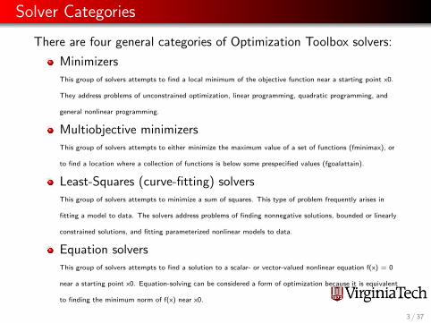
Solver Categories

There are four general categories of Optimization Toolbox solvers:

MinimizersThis group of solvers attempts to find a local minimum of the objective function near a starting point x0.

They address problems of unconstrained optimization, linear programming, quadratic programming, and

general nonlinear programming.

Multiobjective minimizersThis group of solvers attempts to either minimize the maximum value of a set of functions (fminimax), or

to find a location where a collection of functions is below some prespecified values (fgoalattain).

Least-Squares (curve-fitting) solversThis group of solvers attempts to minimize a sum of squares. This type of problem frequently arises in

fitting a model to data. The solvers address problems of finding nonnegative solutions, bounded or linearly

constrained solutions, and fitting parameterized nonlinear models to data.

Equation solversThis group of solvers attempts to find a solution to a scalar- or vector-valued nonlinear equation f(x) = 0

near a starting point x0. Equation-solving can be considered a form of optimization because it is equivalent

to finding the minimum norm of f(x) near x0.

3 / 37

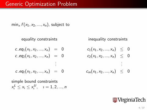
Generic Optimization Problem

minx f (x1, x2, ..., xn), subject to

equality constraints

c eq1(x1, x2, ..., xn) = 0

c eq2(x1, x2, ..., xn) = 0...

c eq`(x1, x2, ..., xn) = 0

inequality constraints

c1(x1, x2, ..., xn) ≤ 0

c2(x1, x2, ..., xn) ≤ 0...

cm(x1, x2, ..., xn) ≤ 0

simple bound constraintsxLı ≤ xı ≤ xU

ı , ı = 1, 2, ..., n

4 / 37

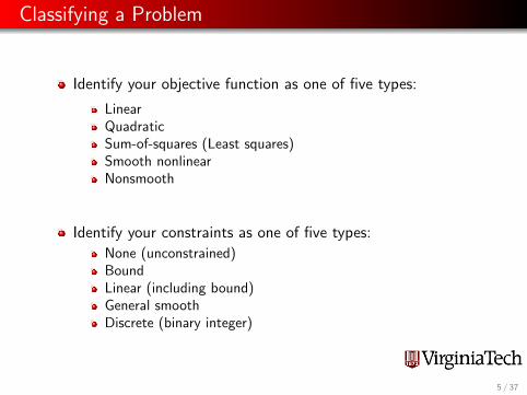
Classifying a Problem

Identify your objective function as one of five types:

LinearQuadraticSum-of-squares (Least squares)Smooth nonlinearNonsmooth

Identify your constraints as one of five types:

None (unconstrained)BoundLinear (including bound)General smoothDiscrete (binary integer)

5 / 37

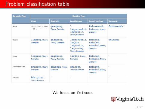
Problem classification table

We focus on fmincon

6 / 37

Matlab’s Optimization Toolbox

Classifying Optimization Problems

A Soup Can Example ⇐

Intermezzo

A Trajectory Example

2nd Trajectory Example: fsolve

7 / 37

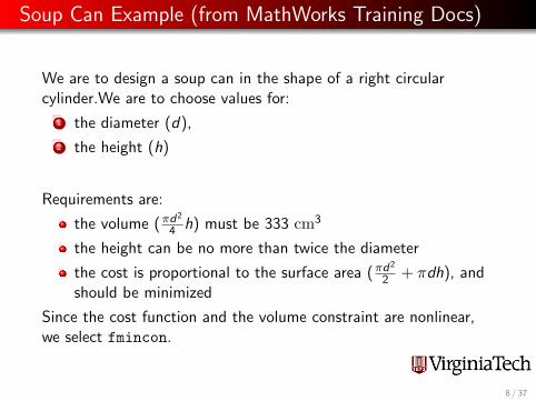
Soup Can Example (from MathWorks Training Docs)

We are to design a soup can in the shape of a right circularcylinder.We are to choose values for:

1 the diameter (d),

2 the height (h)

Requirements are:

the volume (πd2

4 h) must be 333 cm3

the height can be no more than twice the diameter

the cost is proportional to the surface area (πd2

2 + πdh), andshould be minimized

Since the cost function and the volume constraint are nonlinear,we select fmincon.

8 / 37

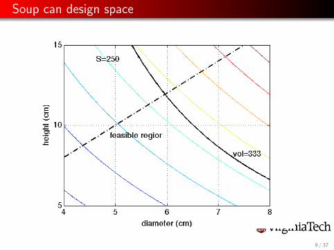
Soup can design space

9 / 37

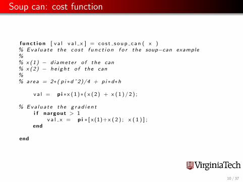
Soup can: cost function

f u n c t i o n [ v a l v a l x ] = c o s t s o u p c a n ( x )% Eva l ua t e the c o s t f u n c t i o n f o r the soup−can example%% x (1) − d i amete r o f the can% x (2) − h e i g h t o f the can%% area = 2∗( p i ∗dˆ2)/4 + p i ∗d∗h

v a l = p i ∗x ( 1 )∗ ( x ( 2 ) + x ( 1 ) / 2 ) ;

% Eva l ua t e the g r a d i e n ti f nargout > 1

v a l x = p i ∗ [ x (1)+ x ( 2 ) ; x ( 1 ) ] ;end

end

10 / 37

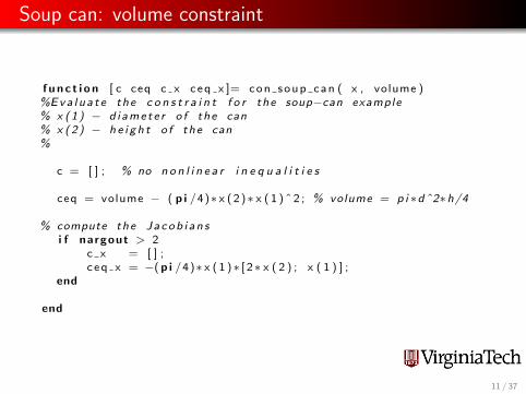
Soup can: volume constraint

f u n c t i o n [ c ceq c x c e q x ]= c o n s o u p c a n ( x , volume )%Eva l ua t e the c o n s t r a i n t f o r the soup−can example% x (1) − d i amete r o f the can% x (2) − h e i g h t o f the can%

c = [ ] ; % no n o n l i n e a r i n e q u a l i t i e s

ceq = volume − ( p i /4)∗ x ( 2 )∗ x ( 1 ) ˆ 2 ; % volume = p i ∗dˆ2∗h/4

% compute the Jacob i an si f nargout > 2

c x = [ ] ;c e q x = −( p i /4)∗ x ( 1 )∗ [ 2∗ x ( 2 ) ; x ( 1 ) ] ;

end

end

11 / 37

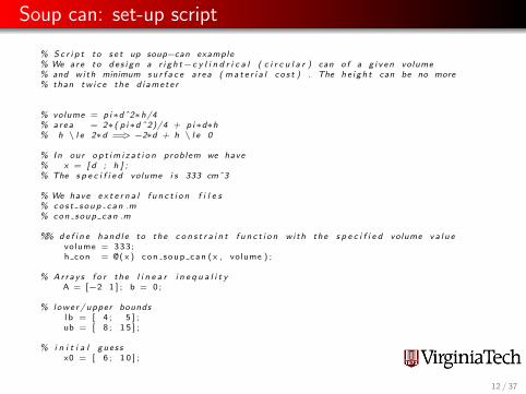
Soup can: set-up script

% Sc r i p t to s e t up soup−can example% We a r e to d e s i g n a r i g h t−c y l i n d r i c a l ( c i r c u l a r ) can o f a g i v en volume% and wi th minimum s u r f a c e a r ea ( ma t e r i a l c o s t ) . The h e i g h t can be no more% than tw i c e the d i amete r

% volume = p i∗dˆ2∗h/4% area = 2∗( p i∗dˆ2)/4 + p i∗d∗h% h \ l e 2∗d ==> −2∗d + h \ l e 0

% In our o p t im i z a t i o n problem we have% x = [ d ; h ] ;% The s p e c i f i e d volume i s 333 cmˆ3

% We have e x t e r n a l f u n c t i o n f i l e s% co s t s o up c an .m% con soup can .m

%% de f i n e hand l e to the c o n s t r a i n t f u n c t i o n wi th the s p e c i f i e d volume va l u evolume = 3 3 3 ;h con = @( x ) c o n s o u p c a n ( x , volume ) ;

% Array s f o r the l i n e a r i n e q u a l i t yA = [−2 1 ] ; b = 0 ;

% lowe r / upper boundsl b = [ 4 ; 5 ] ;ub = [ 8 ; 1 5 ] ;

% i n i t i a l gue s sx0 = [ 6 ; 1 0 ] ;

12 / 37

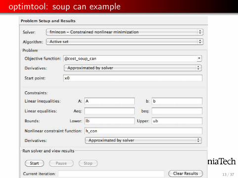
optimtool: soup can example

13 / 37

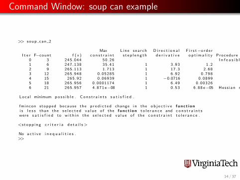
Command Window: soup can example

>> s o u p c a n 2

Max L i n e s e a r c h D i r e c t i o n a l F i r s t−o r d e rI t e r F−count f ( x ) c o n s t r a i n t s t e p l e n g t h d e r i v a t i v e o p t i m a l i t y P r o c e d u r e

0 3 245.044 5 0 . 2 6 I n f e a s i b l e s t a r t p o i n t1 6 247.138 3 5 . 4 1 1 3 . 9 3 1 . 22 9 265.113 1 . 7 1 3 1 1 7 . 3 2 . 6 83 12 265.948 0 .05285 1 6 . 9 2 0 . 7 9 84 15 265 .92 0 .06939 1 −0.0716 0 .08995 18 265.956 0.0001174 1 6 . 4 9 0 .003266 21 265.957 4 . 8 7 1 e−08 1 0 . 5 3 6 . 8 8 e−05 H e s s i a n m o d i f i e d

L o c a l minimum p o s s i b l e . C o n s t r a i n t s s a t i s f i e d .

fmincon s t o p p e d b e c a u s e t h e p r e d i c t e d change i n t h e o b j e c t i v e f u n c t i o ni s l e s s than t h e s e l e c t e d v a l u e o f t h e f u n c t i o n t o l e r a n c e and c o n s t r a i n t swere s a t i s f i e d to w i t h i n t h e s e l e c t e d v a l u e o f t h e c o n s t r a i n t t o l e r a n c e .

<s t o p p i n g c r i t e r i a d e t a i l s >

No a c t i v e i n e q u a l i t i e s .>>

14 / 37

Matlab’s Optimization Toolbox

Classifying Optimization Problems

A Soup Can Example

Intermezzo ⇐

A Trajectory Example

2nd Trajectory Example: fsolve

15 / 37

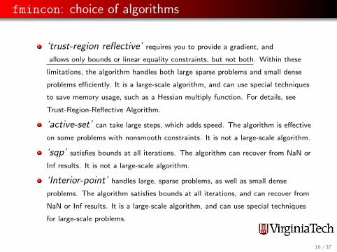
fmincon: choice of algorithms

‘trust-region reflective’ requires you to provide a gradient, and

allows only bounds or linear equality constraints, but not both. Within these

limitations, the algorithm handles both large sparse problems and small dense

problems efficiently. It is a large-scale algorithm, and can use special techniques

to save memory usage, such as a Hessian multiply function. For details, see

Trust-Region-Reflective Algorithm.

‘active-set’ can take large steps, which adds speed. The algorithm is effective

on some problems with nonsmooth constraints. It is not a large-scale algorithm.

‘sqp’ satisfies bounds at all iterations. The algorithm can recover from NaN or

Inf results. It is not a large-scale algorithm.

‘Interior-point’ handles large, sparse problems, as well as small dense

problems. The algorithm satisfies bounds at all iterations, and can recover from

NaN or Inf results. It is a large-scale algorithm, and can use special techniques

for large-scale problems.

16 / 37

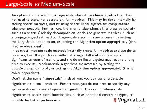
Large-Scale vs Medium-Scale

An optimization algorithm is large scale when it uses linear algebra that doesnot need to store, nor operate on, full matrices. This may be done internally bystoring sparse matrices, and by using sparse linear algebra for computationswhenever possible. Furthermore, the internal algorithms either preserve sparsity,such as a sparse Cholesky decomposition, or do not generate matrices, such asa conjugate gradient method. Large-scale algorithms are accessed by settingthe LargeScale option to on, or setting the Algorithm option appropriately (thisis solver-dependent).In contrast, medium-scale methods internally create full matrices and use denselinear algebra. If a problem is sufficiently large, full matrices take up asignificant amount of memory, and the dense linear algebra may require a longtime to execute. Medium-scale algorithms are accessed by setting theLargeScale option to off, or setting the Algorithm option appropriately (this issolver-dependent).

Don’t let the name ”large-scale” mislead you; you can use a large-scale

algorithm on a small problem. Furthermore, you do not need to specify any

sparse matrices to use a large-scale algorithm. Choose a medium-scale

algorithm to access extra functionality, such as additional constraint types, or

possibly for better performance.

17 / 37

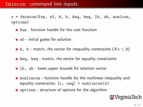
fmincon: command line inputs

x = fmincon(fun, x0, A, b, Aeq, beq, lb, ub, nonlcon,options)

fun - function handle for the cost function

x0 - initial guess for solution

A, b - matrix, rhs vector for inequality constraints (A x ≤ b)

Aeq, beq - matrix, rhs vector for equality constraints

lb, ub - lower,upper bounds for solution vector

nonlincon - function handle for the nonlinear inequality andequality constraints; [c, ceq] = nonlincon(x)

options - structure of options for the algorithm

18 / 37

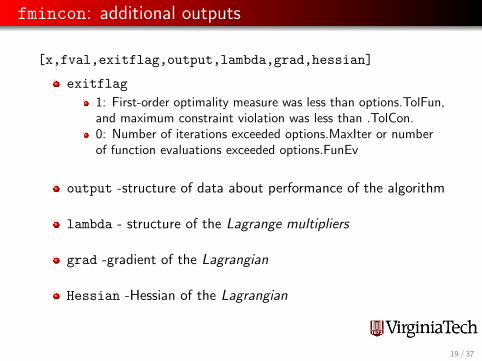
fmincon: additional outputs

[x,fval,exitflag,output,lambda,grad,hessian]

exitflag1: First-order optimality measure was less than options.TolFun,and maximum constraint violation was less than .TolCon.0: Number of iterations exceeded options.MaxIter or numberof function evaluations exceeded options.FunEv

output -structure of data about performance of the algorithm

lambda - structure of the Lagrange multipliers

grad -gradient of the Lagrangian

Hessian -Hessian of the Lagrangian

19 / 37

Matlab’s Optimization Toolbox

Classifying Optimization Problems

A Soup Can Example

Intermezzo

A Trajectory Example ⇐

2nd Trajectory Example: fsolve

20 / 37

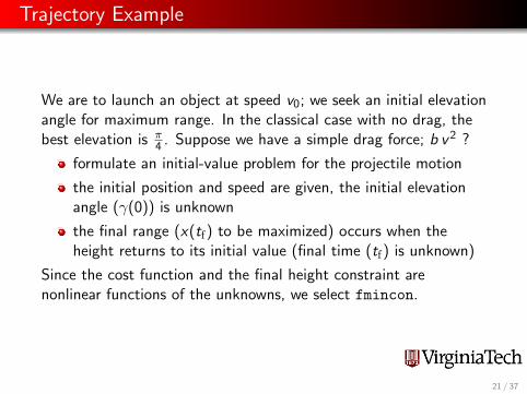
Trajectory Example

We are to launch an object at speed v0; we seek an initial elevationangle for maximum range. In the classical case with no drag, thebest elevation is π

4 . Suppose we have a simple drag force; b v 2 ?

formulate an initial-value problem for the projectile motion

the initial position and speed are given, the initial elevationangle (γ(0)) is unknown

the final range (x(tf) to be maximized) occurs when theheight returns to its initial value (final time (tf) is unknown)

Since the cost function and the final height constraint arenonlinear functions of the unknowns, we select fmincon.

21 / 37

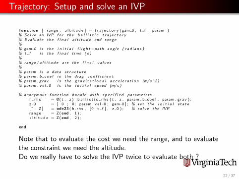
Trajectory: Setup and solve an IVP

f u n c t i o n [ range , a l t i t u d e ] = t r a j e c t o r y ( gam 0 , t f , param )% So l v e an IVP f o r the b a l l i s t i c t r a j e c t o r y% Eva l ua t e the f i n a l a l t i t u d e and range%% gam 0 i s the i n i t i a l f l i g h t−path ang l e ( r a d i a n s )% t f i s the f i n a l t ime ( s )%% range / a l t i t u d e a r e the f i n a l v a l u e s%% param i s a data s t r u c t u r e% param . b c o e f i s the drag c o e f f i c i e n t% param . g rav i s the g r a v i t a t i o n a l a c c e l e r a t i o n (m/ s ˆ2)% param . v e l 0 i s the i n i t i a l speed (m/ s )

% anonymous f u n c t i o n hand l e w i th s p e c i f i e d pa ramete r sh r h s = @( t , z ) b a l l i s t i c r h s ( t , z , param . b c o e f , param . g r a v ) ;z 0 = [ 0 ; 0 ; param . v e l 0 ; gam 0 ] ; % se t the i n i t i a l s t a t e[ ˜ , Z ] = ode23 ( h r h s , [ 0 t f ] , z 0 ) ; % so l v e the IVPr a n g e = Z( end , 1 ) ;a l t i t u d e = Z( end , 2 ) ;

end

Note that to evaluate the cost we need the range, and to evaluatethe constraint we need the altitude.Do we really have to solve the IVP twice to evaluate both ?

22 / 37

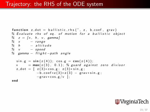
Trajectory: the RHS of the ODE system

f u n c t i o n z d o t = b a l l i s t i c r h s ( ˜ , z , b c o e f , g r a v )% Eva l ua t e r h s o f eq . o f motion f o r a b a l l i s t i c o b j e c t% z = [ x , h , v , gamma ]% x − range% h − a l t i t u d e% v − speed% gamma − f l i g h t −path ang l e

s i n g = s i n ( z ( 4 ) ) ; c o s g = cos ( z ( 4 ) ) ;v = max( z ( 3 ) , 0 . 1 ) ; % guard a g a i n s t z e r o d i v i s o rz d o t = [ z ( 3 )∗ c o s g ; z ( 3 )∗ s i n g ;

−b c o e f ∗ z ( 3 )∗ z ( 3 ) − g r a v ∗ s i n g ;−g r a v ∗ c o s g / v ] ;

end

23 / 37

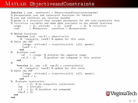
Matlab: ObjectiveandConstraints

f u n c t i o n [ cos t , n o n l i n c o n ] = O b j e c t i v e a n d C o n s t r a i n t s ( param )% Encap su l a t e s c o s t and c o n s t r a i n t f u n c t i o n s f o r fmincon% co s t and non l i n c on a r e f u n c t i o n hand l e s% param i s a s t r u c t u r e tha t encodes pa ramete r s f o r the c o s t / c o n s t r a i n t f c n s% I n i t i a l i z e v a r i a b l e s and make them a v a i l a b l e to the ne s t ed f u n c t i o n s

r a n g e = [ ] ; a l t i t u d e = [ ] ; LastZ = [ ] ; % i n i t i a l i z ec o s t = @ o b j e c t i v e ; n o n l i n c o n = @ c o n s t r a i n t s ;

% Nested f u n c t i o n sf u n c t i o n [ v a l , v a l Z ] = o b j e c t i v e ( z )

i f ˜ i s e q u a l ( z , LastZ ) % update f o r t h i s v a l u e% So l v e the IVP

[ range , a l t i t u d e ] = t r a j e c t o r y ( z ( 1 ) , z ( 2 ) , param ) ;LastZ = z ;

end% Eva l ua t e c o s t

v a l = −r a n g e ; % min imize the n e g a t i v e rangev a l Z = [ ] ; % g r a d i e n t not computed i n t h i s v e r s i o n

end%

f u n c t i o n [ c , ceq c Z , ceq Z ] = c o n s t r a i n t s ( z )i f ˜ i s e q u a l ( z , LastZ ) % update f o r t h i s v a l u e

% So l v e the IVP[ range , a l t i t u d e ] = t r a j e c t o r y ( z ( 1 ) , z ( 2 ) , param ) ;LastZ = z ;

end% Eva l ua t e c o n s t r a i n t s

c = [ ] ; % no i n e q u a l i t y c o n s t r a i n t sceq = a l t i t u d e ;c Z = [ ] ; % Jacob i an s not computedceq Z = [ ] ;

endend

24 / 37

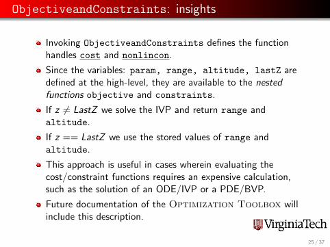
ObjectiveandConstraints: insights

Invoking ObjectiveandConstraints defines the functionhandles cost and nonlincon.

Since the variables: param, range, altitude, lastZ aredefined at the high-level, they are available to the nestedfunctions objective and constraints.

If z 6= LastZ we solve the IVP and return range andaltitude.

If z == LastZ we use the stored values of range andaltitude.

This approach is useful in cases wherein evaluating thecost/constraint functions requires an expensive calculation,such as the solution of an ODE/IVP or a PDE/BVP.

Future documentation of the Optimization Toolbox willinclude this description.

25 / 37

fmincon:trajectory example

% Sc r i p t to s e t pa ramete r s f o r and then run the max−range t r a j e c t o r y problem%% param i s a s t r u c t u r e o f data f o r the problem% param . b c o e f i s the drag c o e f f i c i e n t% param . g rav i s the g r a v i t a t i o n a l a c c e l e r a t i o n (m/ s ˆ2)% param . v e l 0 i s the i n i t i a l speed (m/ s )

param . b c o e f = 0 . 1 ;param . g r a v = 9 . 8 ;param . v e l 0 = 2 5 . 0 ;

% de f i n e hand l e s f o r f u n c t i o n s e v a l u a t i n g the co s t / c o n t r a i n t s

[ cos t , n o n l c o n ] = O b j e c t i v e a n d C o n s t r a i n t s ( param ) ;

% lowe r / upper boundsl b = [ 0 ; 0.5∗ param . v e l 0 /param . g r a v ] ;ub = [ p i / 4 ; 5∗ l b ( 2 ) ] ;

% i n i t i a l gue s sx0 = 0 . 5∗ ( l b+ub ) ;

%% se t pa ramete r s and i n voke fminconOPT = o p t i m s e t ( ’ fmincon ’ ) ;OPT = o p t i m s e t (OPT, ’ A l g o r i t h m ’ , ’ a c t i v e−s e t ’ , . . .

’ D i s p l a y ’ , ’ i t e r ’ , . . .’ U s e P a r a l l e l ’ , ’ a l w a y s ’ ) ;

% x s t a r = fmincon ( fun , x0 , A , b ,Aeq , beq , lb , ub , nonlcon , o p t i o n s )x s t a r = fmincon ( cost , x0 , [ ] , [ ] , [ ] , [ ] , lb , ub , nonlcon , OPT) ;

26 / 37

Matlab’s Optimization Toolbox

Classifying Optimization Problems

A Soup Can Example

Intermezzo

A Trajectory Example

2nd Trajectory Example: fsolve ⇐

27 / 37

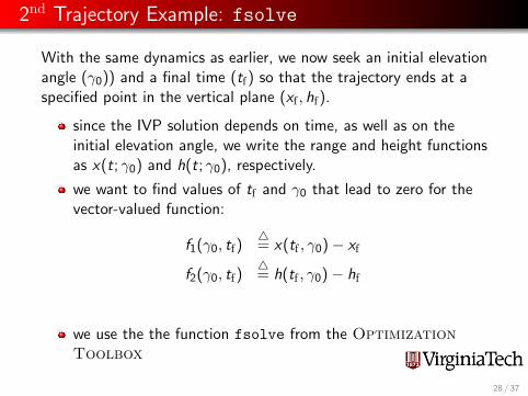
2nd Trajectory Example: fsolve

With the same dynamics as earlier, we now seek an initial elevationangle (γ0)) and a final time (tf) so that the trajectory ends at aspecified point in the vertical plane (xf , hf).

since the IVP solution depends on time, as well as on theinitial elevation angle, we write the range and height functionsas x(t; γ0) and h(t; γ0), respectively.

we want to find values of tf and γ0 that lead to zero for thevector-valued function:

f1(γ0, tf)4= x(tf , γ0)− xf

f2(γ0, tf)4= h(tf , γ0)− hf

we use the the function fsolve from the OptimizationToolbox

28 / 37

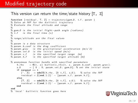
Modified trajectory code

This version can return the time/state history [T, Z]

f u n c t i o n [ r e s i d u a l , T, Z ] = t r a j e c t o r y ( gam 0 , t f , param )% So l v e an IVP f o r the b a l l i s t i c t r a j e c t o r y% Eva l ua t e the f i n a l a l t i t u d e and range%% gam 0 i s the i n i t i a l f l i g h t−path ang l e ( r a d i a n s )% t f i s the f i n a l t ime ( s )%% range / a l t i t u d e a r e the f i n a l v a l u e s%% param i s a data s t r u c t u r e% param . b c o e f i s the drag c o e f f i c i e n t% param . g rav i s the g r a v i t a t i o n a l a c c e l e r a t i o n (m/ s ˆ2)% param . v e l 0 i s the i n i t i a l speed (m/ s )% param . x f i s the s p e c i f i e d t a r g e t range (m)% param . h f i s the s p e c i f i e d t a r g e t a l t i t u d e (m)

% anonymous f u n c t i o n hand l e w i th s p e c i f i e d pa ramete r sh r h s = @( t , z ) b a l l i s t i c r h s ( t , z , param . b c o e f , param . g r a v ) ;z 0 = [ 0 ; 0 ; param . v e l 0 ; gam 0 ] ; % se t the i n i t i a l s t a t ei f nargout == 1

[ ˜ , Z ] = ode23 ( h r h s , [ 0 t f ] , z 0 ) ; % so l v e the IVPr e s i d u a l = Z( end , 1 : 2 ) ’ − [ param . x f ; param . h f ] ;

e l s e[ T, Z ] = ode23 ( h r h s , [ 0 t f ] , z 0 ) ; % so l v e the IVPr e s i d u a l = Z( end , 1 : 2 ) ’ − [ param . x f ; param . h f ] ;

endend% ’ l o c a l ’ b a l l i s t i c f u n c t i o n goes he r e

29 / 37

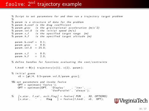
fsolve: 2nd trajectory example

% Sc r i p t to s e t pa ramete r s f o r and then run a t r a j e c t o r y t a r g e t problem%% param i s a s t r u c t u r e o f data f o r the problem% param . b c o e f i s the drag c o e f f i c i e n t% param . g rav i s the g r a v i t a t i o n a l a c c e l e r a t i o n (m/ s ˆ2)% param . v e l 0 i s the i n i t i a l speed (m/ s )% param . x f i s the s p e c i f i e d t a r g e t range (m)% param . h f i s the s p e c i f i e d t a r g e t a l t i t u d e (m)

param . b c o e f = 0 . 1 ;param . g r a v = 9 . 8 ;param . v e l 0 = 2 5 . 0 ;

param . x f = 8 . 0 ;param . h f = 2 . 0 ;

% de f i n e hand l e s f o r f u n c t i o n s e v a l u a t i n g the co s t / c o n t r a i n t s

f h n d l = @( x ) t r a j e c t o r y ( x ( 1 ) , x ( 2 ) , param ) ;

% i n i t i a l gue s sx0 = [ p i / 4 ; 0.5∗ param . v e l 0 /param . g r a v ] ;

%% se t pa ramete r s and i n voke f s o l v eOPT = o p t i m s e t ( ’ f s o l v e ’ ) ;OPT = o p t i m s e t (OPT, ’ D i s p l a y ’ , ’ i t e r ’ , . . .

’ U s e P a r a l l e l ’ , ’ a l w a y s ’ ) ;

% [ x s t a r , f v a l , e x i t f l a g ] = f s o l v e ( FUN , X0 , OPTIONS)[ x s t a r , ˜ , f l a g ] = f s o l v e ( f h n d l , x0 , OPT) ;

30 / 37

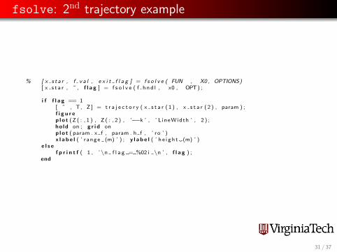
fsolve: 2nd trajectory example

% [ x s t a r , f v a l , e x i t f l a g ] = f s o l v e ( FUN , X0 , OPTIONS)[ x s t a r , ˜ , f l a g ] = f s o l v e ( f h n d l , x0 , OPT) ;

i f f l a g == 1[ ˜ , T, Z ] = t r a j e c t o r y ( x s t a r ( 1 ) , x s t a r ( 2 ) , param ) ;f i g u r ep l o t (Z ( : , 1 ) , Z ( : , 2 ) , ’−−k ’ , ’ L ineWidth ’ , 2 ) ;ho ld on ; g r i d onp l o t ( param . x f , param . h f , ’ r o ’ )x l a b e l ( ’ r a n g e (m) ’ ) ; y l a b e l ( ’ h e i g h t (m) ’ )

e l s ef p r i n t f ( 1 , ’\n f l a g = %02 i \n ’ , f l a g ) ;

end

31 / 37

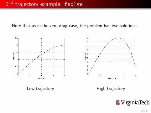
2nd trajectory example: fsolve

Note that as in the zero-drag case, the problem has two solutions

Low trajectory High trajectory

32 / 37

THE END

Please complete the evaluation formhttp://www.fdi.vt.edu/training/evals/

Thanks

33 / 37

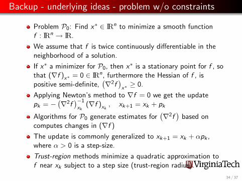
Backup - underlying ideas - problem w/o constraints

Problem P0: Find x∗ ∈ IRn to minimize a smooth functionf : IRn → IR.

We assume that f is twice continuously differentiable in theneighborhood of a solution.

If x∗ a minimizer for P0, then x∗ is a stationary point for f , sothat (∇f )x∗ = 0 ∈ IRn, furthermore the Hessian of f , ispositive semi-definite,

(∇2f

)x∗≥ 0.

Applying Newton’s method to ∇f = 0 we get the updatepk = −

(∇2f

)−1

xk(∇f )xk

, xk+1 = xk + pk

Algorithms for P0 generate estimates for(∇2f

)based on

computes changes in (∇f )

The update is commonly generalized to xk+1 = xk + αpk ,where α > 0 is a step-size.

Trust-region methods minimize a quadratic approximation tof near xk subject to a step size (trust-region radius).

34 / 37

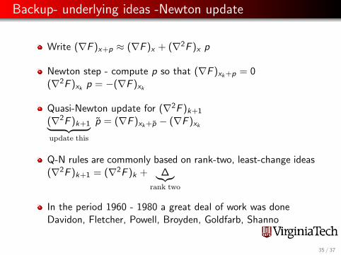
Backup- underlying ideas -Newton update

Write (∇F )x+p ≈ (∇F )x + (∇2F )x p

Newton step - compute p so that (∇F )xk+p = 0(∇2F )xk

p = −(∇F )xk

Quasi-Newton update for (∇2F )k+1

(∇2F )k+1︸ ︷︷ ︸update this

p̃ = (∇F )xk+p̃ − (∇F )xk

Q-N rules are commonly based on rank-two, least-change ideas(∇2F )k+1 = (∇2F )k + ∆︸︷︷︸

rank two

In the period 1960 - 1980 a great deal of work was doneDavidon, Fletcher, Powell, Broyden, Goldfarb, Shanno

35 / 37

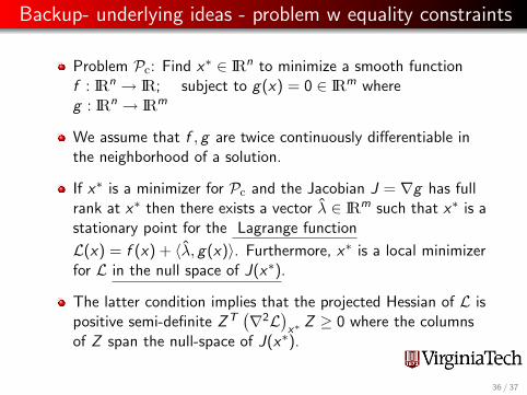
Backup- underlying ideas - problem w equality constraints

Problem Pc: Find x∗ ∈ IRn to minimize a smooth functionf : IRn → IR; subject to g(x) = 0 ∈ IRm whereg : IRn → IRm

We assume that f , g are twice continuously differentiable inthe neighborhood of a solution.

If x∗ is a minimizer for Pc and the Jacobian J = ∇g has fullrank at x∗ then there exists a vector λ̂ ∈ IRm such that x∗ is astationary point for the Lagrange function

L(x) = f (x) + 〈λ̂, g(x)〉. Furthermore, x∗ is a local minimizerfor L in the null space of J(x∗).

The latter condition implies that the projected Hessian of L ispositive semi-definite ZT

(∇2L

)x∗

Z ≥ 0 where the columnsof Z span the null-space of J(x∗).

36 / 37

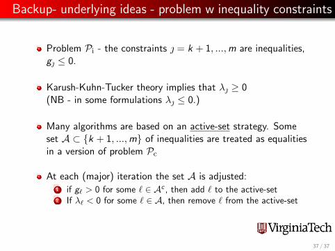
Backup- underlying ideas - problem w inequality constraints

Problem Pi - the constraints = k + 1, ...,m are inequalities,g ≤ 0.

Karush-Kuhn-Tucker theory implies that λ ≥ 0(NB - in some formulations λ ≤ 0.)

Many algorithms are based on an active-set strategy. Someset A ⊂ {k + 1, ...,m} of inequalities are treated as equalitiesin a version of problem Pc

At each (major) iteration the set A is adjusted:1 if g` > 0 for some ` ∈ Ac , then add ` to the active-set2 If λ` < 0 for some ` ∈ A, then remove ` from the active-set

37 / 37