MATILDA TEHLER Modeling Phase Transformations and …274821/FULLTEXT02.pdf · MATILDA TEHLER...
50
Modeling Phase Transformations and Volume Changes during Cooling of Case Hardening Steels MATILDA TEHLER Licentiate Thesis in Materials Science and Engineering Stockholm, Sweden 2009
Transcript of MATILDA TEHLER Modeling Phase Transformations and …274821/FULLTEXT02.pdf · MATILDA TEHLER...
ISRN KTH/MSE--09/47--SE+MEK/AVHISBN 978-91-7415-459-7
www.kth.se
MA
TILDA
TEHLER
Modeling Phase Transform
ations and Volume Changes during Cooling of Case Hardening Steels
Modeling Phase Transformationsand Volume Changes during Cooling
of Case Hardening Steels
M A T I L D A T E H L E R
KTH 2009
Licentiate Thesis inMaterials Science and Engineering
Stockholm, Sweden 2009

Modeling Phase Transformations and Volume Changes during Cooling of Case Hardening Steels
Matilda Tehler
Licentiate Thesis
Department of Materials Science and Engineering Royal Institute of Technology, KTH
Stockholm, Sweden, 2009

II
Copyright © 2009 Matilda Tehler ISRN KTH/MSE--09/47--SE+MEK/AVH ISBN 978-91-7415-459-7 Department of Materials Science and Engineering Royal Institute of Technology, KTH SE-100 44 Stockholm, Sweden
III
Abstract Case hardening distortions are a major problem for gear manufacturers. The aim of the current work is to create a simulation model, able to predict how and when case hardening distortions arise. The results presented in this thesis form a basis for such a model.
Two case hardening steels, with base carbon contents of 0.20 and 0.21 % C were studied using dilatometer experiments. One of them was carburized to 0.36, 0.52 and 0.65 % C in order to investigate the influence of carbon content. Experiments were performed during both isothermal and continuous heating and cooling conditions. The results were used to evaluate phase transforma-tions, heat expansion behaviors and phase transformation strains. The expansion behavior of the material was modeled as a function of temperature, carbon content and phase fractions. The phase transformations to martensite and bainite were modeled, using the Koistinen-Marburger equation and a transformation rate equation based on Austin-Rickett kinetics, respectively. Experiments were simulated using the COMSOL Multiphysics software, to verify the model with respect to martensite and bainite transformations, heat expansion behavior and phase transformation strains.

IV
V
Preface The work this licentiate thesis is based on was performed at the department of Materials Science and Technology at the Royal Institute of Technology, KTH, Stockholm Sweden, and supervised by Professor Stefan Jonsson. It is part of the project OPTIMA - Case Hardening Steel, financed by VINNOVA and KTH-DMMS, and was performed in collaboration with Chalmers University of Technology, Volvo Powertrain AB, Scania CV AB, Componenta Wirsbo AB and Arvin Meritor. Jernkontoret and the A H Göranssons Fund are gratefully acknowledged for their generous support.
List of Papers This thesis is based on the following appended papers.
1. A Material Model for Simulating Volume Changes during Phase Transformations Proceedings of the COMSOL Users Conference 2007 Grenoble, 2 (2007) pp. 648-653.
2. Modeling Bainitic Transformation in a Case Hardening Steel To be submitted.
3. Modeling Volume Changes during Cooling of Case Hardening Steels To be submitted.

VI
VII
Description of Papers
1. A Material Model for Simulating Volume Changes during Phase Transformations
This is a contribution to the COMSOL Users Conference 2007 in Grenoble, and describes how COMSOL Multiphysics is used to simulate dilalometer experiments. A first attempt to describe time dependent phase transformations is presented. However, it was later discovered that the parameters for the transformation-rate equation are dependent on the heating rate. Thus, a new rate-independent phase transformation equation was later developed, described in Supplement 2.
2. Modeling Bainitic Transformation in a Case Hardening Steel The paper contains experimental and simulated results for the phase transformation of austenite to bainite during isothermal conditions. A case hardening steel is studied at four carbon contents, using a dilatometer. The bainite fraction is calculated by time integration of a time-independent transformation rate equation, derived from Austin-Rickett kinetics. Simulations in COMSOL Multiphysics produces bainite fractions correlating to experiments.
3. Modeling Volume Changes during Cooling of Case Hardening Steels
Results regarding martensitic and bainitic phase transformations, heat expansion behaviors and phase transformation strains during constant heating and cooling rates are presented. Equations describing heat expansion behavior, phase transformation strain and martensitic formation are evaluated as functions of carbon content. The equation for bainitic transformation described in Supplement 2 is used during constant cooling rates for two different case hardening steels. COMSOL Multiphysics is used to simulate experiments, producing good agreement between experimental and simulated dilatometer curves.
Contributions from the Author Supplement 1. All calculations and evaluations of model parameters were performed by Tehler. The manuscript was written together with Jonsson. Tehler presented the work at the COMSOL Users Conference in Grenoble.
Supplement 2 and 3. Planning of experimental work, analyses of data, evaluations of model parameters and all calculations were performed by Tehler. The complete manuscript was written by Tehler and revised together with Jonsson.

VIII
IX
Table of Contents
1 Introduction 1 1.1 The Origin of Distortions 1 1.2 Outline and Aim of the Work 2
2 Modeling Phase Transformations and Volume Changes 5 2.1 Time Dependent Transformations 5 2.2 Deriving a Rate Equation for Time Dependent Transformations 5 2.3 The Martensitic Transformation 6 2.4 Heat Expansion Behavior and Phase Transformation Strain 7 2.5 Simulation of Dilatometer Experiments 7
3 Experimental Work 9 3.1 Material 9 3.2 Heat Treatment 10 3.3 Evaluation of Isothermal Phase Fractions 10 3.4 Isothermal Decomposition of Austenite 11
3.4.1 Bainitic Transformation 11 3.4.2 Decomposition of Austenite at High Temperatures 14
3.5 Isothermal Austenitization 16 3.6 Constant Heating and Cooling Rates 18
4 Evaluation of Model Parameters 21 4.1 AR-Parameters for the Bainitic Transformation 21 4.2 Parameters for the Martensitic Transformation 22 4.3 Heat Expansion Behavior 23 4.4 Two Phase Region with Austenite and Ferrite 24
5 Results and Discussion 27 5.1 Isothermal Bainitic Transformation 27 5.2 Cooling Curves 28
6 Conclusions 31 7 Future Work 33

X
1
1 Introduction The gear box of a heavy vehicle contains a large number of gears. The toler-ances for the gears are very fine, thus the requirements during manufacturing are extremely high. Gears that do not meet the requirements will either be machined further, or scrapped, both alternatives creating large costs for the manufacturer. Unpredictable hardening distortions of transmission gears are a major problem. Hence, understanding the origin of distortions is important and can help the manufacturer to optimize the manufacturing process in order to reduce distortions.
The desired mechanical properties of a gear is a hard, wear and fatigue resistant surface and a tough interior, to withstand the load applied during use. To obtain these properties, gears are case hardened. A large part of the distortion that appears during manufacturing arises during the case hardening process. Thus, a simulation model able to predict case hardening distortions is a valuable tool for predicting ways to reduce and control distortions.
1.1 The Origin of Distortions To understand the origin of the distortions it is important to understand the manufacturing process. The manufacturing of gears starts at a steel plant, where the steel melt is continuously cast into billets. The billets are then divided into smaller pieces, which are forged in several steps to blanks, slightly larger than the finished gear. The forged blanks are given a ferritic-pearlitic microstructure by controlled cooling. They are then machined in many steps to a final shape where the expected shape changes during subsequent hardening are compensated for. All steps of the manufacturing process, in combination with the material properties of the steel and the geometry of the gear, will determine the final distortion of the finished gear. As these distortions are stochastic in magnitude and direction, they cannot be compensated for during soft machining.
In general, all non-uniformities in both gear geometry and microstructure results in a more distortion sensitive part. Mallener1 describes the effect of gear geometry on the distortions. For example, a large gear with a thin wall thick-ness is much more likely to distort than a smaller more compact gear. All non-uniformities in the microstructure increase the risk of non-uniform phase transformations, which is a potential source of distortion due to the volume differences between the different phases. Hence, non-uniform phase transfor-mations lead to non-uniform volume changes in the material. If the stresses from the volume changes exceed the yield strength of the material, it will deform plastically, resulting in distortions. The transformation temperatures for martensite depend on the chemical composition, the austenite grain size
2
and the stress distribution in the material. Decreased austenite grain size, increased carbon content and increased hydrostatic pressure lower the marten-sitic start temperature2, 3, 4. Hence, non-uniformities in chemical composition, grain size and internal stresses results in non-uniform martensite phase trans-formation. Non-uniform material properties are therefore a possible source of distortions.
The casting, forging and machining processes determines the distribution of segregated alloying elements, non-uniformities in the microstructure and the residual stress distributions in the part, three possible reasons for distortion5. The microstructure obtained during casting does not disappear during forging. Mallener1 describes the effect of the casting geometry on distortion in crown wheals, originally published by Seger. He found that a rectangular casting geometry results in an oval gear shape, while a squared casting geometry results in a square-shaped gear, concluding that minimized distortion can be obtained by using a cylindrical, continuously cast shape.
Finally, conditions during hardening affect the distortion in the finished gear, especially during non-uniform heating and cooling conditions. The tempera-ture difference during heating is much smaller than the temperature difference during quenching, hence the distortion from thermal stresses during heating is, according to Sturm et al.6, usually lower than the distortion from thermal stresses during quenching. However, some stresses are induced in the material during the ferrite-pearlite to austenite transformation. Since the material can easily deform plastically during austenitizing, due to the low yield stress at such high temperature, even relatively small stresses can result in distortion due to plastic deformation. Hence, Kessler et al.5 state that the method of heating to the carburizing temperature can have a greater influence on the distortion than the quenching factors. In addition, Canale and Totten4, claims that the prime cause of quench distortion is non-uniform cooling from the austenitizing temperature. Non-uniform cooling can arise from a non-uniform flow field or non-uniform wetting of one surface of the gear.
In summary, in order to reduce hardening distortions, the manufacturing process and the material properties should be as axisymmetrical and homoge-neous as possible.
1.2 Outline and Aim of the Work The aim of the current work is to develop a simulation model able to predict exactly how and when during case hardening, distortions arise. The develop-ment of the model is divided into two steps. As a first step, the phase trans-formation and heat expansion behavior during hardening is calculated. In the second step, plastic deformation generated by the first step is included in the
3
model, making it possible to calculate distortions. This licentiate thesis is focusing on the first step. The model parameters during this step are evaluated from dilatometry experiments, which are also used to verify the simulated results.
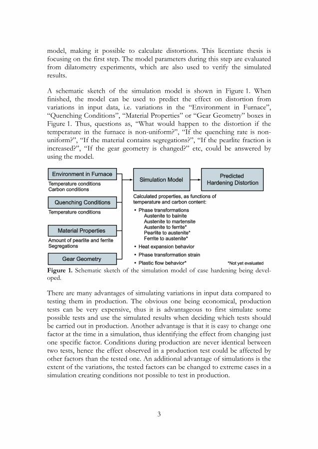
A schematic sketch of the simulation model is shown in Figure 1. When finished, the model can be used to predict the effect on distortion from variations in input data, i.e. variations in the “Environment in Furnace”, “Quenching Conditions”, “Material Properties” or “Gear Geometry” boxes in Figure 1. Thus, questions as, “What would happen to the distortion if the temperature in the furnace is non-uniform?”, “If the quenching rate is non-uniform?”, “If the material contains segregations?”, “If the pearlite fraction is increased?”, “If the gear geometry is changed?” etc, could be answered by using the model.
Figure 1. Schematic sketch of the simulation model of case hardening being devel-oped.
There are many advantages of simulating variations in input data compared to testing them in production. The obvious one being economical, production tests can be very expensive, thus it is advantageous to first simulate some possible tests and use the simulated results when deciding which tests should be carried out in production. Another advantage is that it is easy to change one factor at the time in a simulation, thus identifying the effect from changing just one specific factor. Conditions during production are never identical between two tests, hence the effect observed in a production test could be affected by other factors than the tested one. An additional advantage of simulations is the extent of the variations, the tested factors can be changed to extreme cases in a simulation creating conditions not possible to test in production.

4
5
2 Modeling Phase Transformations and Volume Changes
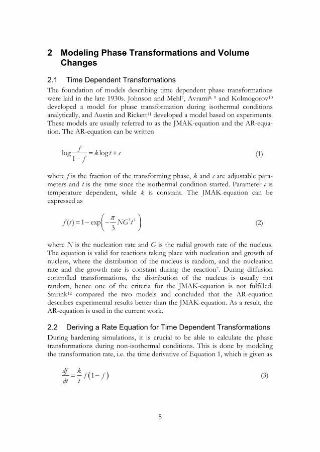
2.1 Time Dependent Transformations The foundation of models describing time dependent phase transformations were laid in the late 1930s. Johnson and Mehl7, Avrami8, 9 and Kolmogorov10 developed a model for phase transformation during isothermal conditions analytically, and Austin and Rickett11 developed a model based on experiments. These models are usually referred to as the JMAK-equation and the AR-equa-tion. The AR-equation can be written
log log1
f k t cf= +
− (1)
where f is the fraction of the transforming phase, k and c are adjustable para-meters and t is the time since the isothermal condition started. Parameter c is temperature dependent, while k is constant. The JMAK-equation can be expressed as
3 4( ) 1 exp3
f t NG tπ⎛ ⎞= − −⎜ ⎟⎝ ⎠
(2)
where N is the nucleation rate and G is the radial growth rate of the nucleus. The equation is valid for reactions taking place with nucleation and growth of nucleus, where the distribution of the nucleus is random, and the nucleation rate and the growth rate is constant during the reaction7. During diffusion controlled transformations, the distribution of the nucleus is usually not random, hence one of the criteria for the JMAK-equation is not fulfilled. Starink12 compared the two models and concluded that the AR-equation describes experimental results better than the JMAK-equation. As a result, the AR-equation is used in the current work.
2.2 Deriving a Rate Equation for Time Dependent Transformations During hardening simulations, it is crucial to be able to calculate the phase transformations during non-isothermal conditions. This is done by modeling the transformation rate, i.e. the time derivative of Equation 1, which is given as
( )1df k f fdt t
= − (3)
6
By solving Equation 1 for t and substituting it in Equation 3, a rate function of f and T is obtained as
( )1 1// 1 1/10 1 kc k kdf k f fdt
+−= ⋅ ⋅ ⋅ − (4)
where the temperature dependence is hidden in the c-parameter. During a simulation of a phase transformation, the phase fraction, f, is calculated by time integration of Equation 4. Two problems are then encountered. One is that the transformation rate is zero at the beginning of the transformation, when f = 0. The second is that the transformation rate becomes zero when the trans-formed fraction is one, which is only valid in one-phase regions. In two-phase regions the transformation rate should be zero as the equilibrium fraction, flimit, is reached. In order to solve these problems, Equation 4 is modified according to
( ) ( )1 1/1 1//10 'kkc k
limitdf k f f fdt
+−= ⋅ ⋅ ⋅ − (5)
where
, for >0.0001,'
0.0001 otherwise.f f
f⎧
= ⎨⎩
i.e. a nucleation fraction of 0.0001 is adopted and the transformation is limited by the equilibrium fraction at the end of the transformation. This rate equation appears to be valid for any heat treating condition. In the present work, it is used to calculate the bainitic transformation during isothermal and continuous cooling conditions.
2.3 The Martensitic Transformation Koistinen and Marburger13 developed an equation for the diffusionless transformation from austenite to martensite, where the fraction of martensite, fα’, is calculated as
( )( )' 1 - exp - - , for s sf a M T T Mα = ⋅ < (6)
where a is an adjustable parameter, Ms is the martensitic start temperature and T is the temperature in Kelvin. The equation was developed for pure iron carbon alloys during the austenite to martensite transformation without the presence of other phases, i.e. for quenching. In order to account for the
7
presence of other phases, formed during lower cooling rates, the equation used in the simulations is modified by multiplying with the fraction of austenite retained at Ms, (1-∑fi ), where the summation is carried out over all phases, except martensite and austenite. The modified equation is thus
( )( )( ) ( )'
1 - exp - - 1 , for ,
0, otherwise.s i sa M T f T M
fα⎧ ⋅ ⋅ − <⎪= ⎨⎪⎩
∑ (7)
2.4 Heat Expansion Behavior and Phase Transformation Strain Different phases have different heat expansion behaviors. The equations used to describe the heat expansions for the different phases and structures were directly evaluated from the dilatometer curves by fitting polynomials of temperature and carbon content to the experimental data. The volume changes during phase transformations were calculated by following the linear combina-tion of the contributions of the individual phases. Thus, if e.g. the material consists of 50 % austenite and 50 % martensite, the heat expansion for the material is half-way between the martensite and the austenite heat expansion lines. The transformation strain during phase transformations are thereby automatically described, as the material changes its heat expansion behavior to follow the behavior of the new phase formed. The total strain in the material from both heat expansion and phase transformations, as a function of temper-ature and carbon content, ε(T,C ), is thus
( , ) ( , )i iT C T C fε ε= ⋅∑ (8)
where i represents the phases and structures ferrite, pearlite, austenite, bainite and martensite. Equation 8 represents the one-dimensional strain. By assuming isotropic behavior, the three-dimensional strain was calculated using the same equation for every dimension.
2.5 Simulation of Dilatometer Experiments The aim of the current work is to develop a model of the entire case hardening process, able to predict how and when hardening distortions arise. The model is developed using the software COMSOL Multiphysics14, which is a finite element software specialized in solving problems composed of a number of different physical sub-problems. COMSOL Multiphysics is divided into differ-ent modules, where every module is specialized in different types of physical problems, i.e. “Heat Transfer”, “Structural Mechanics”, “Convection and Diffusion” etc. The modules can be combined in any combination to make a good platform for solving many types of problems.
8
The base for the current model is the predefined modules “General Heat Transfer” and “Axial Symmetry, Stress-Strain”. By combining these two modules, the temperature conditions during hardening and the resulting mechanical response can be calculated. COMSOL Multiphysics does, however, not predict the phase transformations occurring during hardening. Thus, the equations for calculating phase transformations and heat expansion for the different phases, described earlier, were added. In the current work the model was used to simulate dilatometer experiments in order to validate it with respect to heat expansion, bainite and martensite formation and phase transformation strain. The simulation procedure is described further in Supplement 1.
9
3 Experimental Work Phase transformation kinetics, heat expansion behavior and phase transforma-tion strain were studied using dilatometer experiments. A dilatometer consists of a vacuum chamber where a specimen is clamped between two long supports, generally made of silica with low thermal expansion. An induction coil around the specimen heats it at a controlled rate whereas the length changes are recorded by the movements of the silica rods. The time tempera-ture history can be precisely controlled with prescribed heating and cooling rates and with prescribed hold temperatures and times. The heating rates can be very high, whereas high cooling rates can only be achieved by gas quenching which disturbs the recorded data. A typical specimen is a solid cylinder 10 mm high, with a diameter of 4 mm.
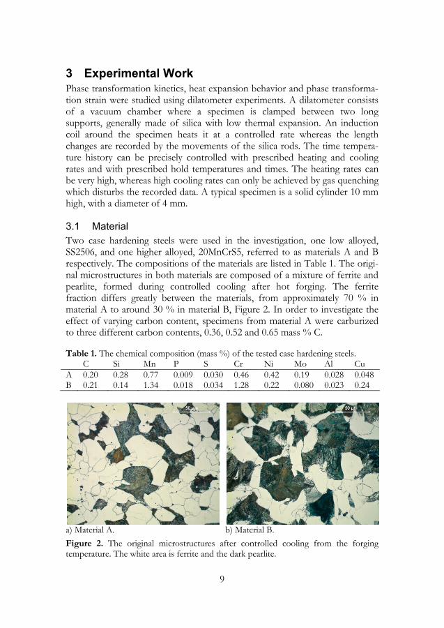
3.1 Material Two case hardening steels were used in the investigation, one low alloyed, SS2506, and one higher alloyed, 20MnCrS5, referred to as materials A and B respectively. The compositions of the materials are listed in Table 1. The origi-nal microstructures in both materials are composed of a mixture of ferrite and pearlite, formed during controlled cooling after hot forging. The ferrite fraction differs greatly between the materials, from approximately 70 % in material A to around 30 % in material B, Figure 2. In order to investigate the effect of varying carbon content, specimens from material A were carburized to three different carbon contents, 0.36, 0.52 and 0.65 mass % C.
Table 1. The chemical composition (mass %) of the tested case hardening steels. C Si Mn P S Cr Ni Mo Al Cu A 0.20 0.28 0.77 0.009 0.030 0.46 0.42 0.19 0.028 0.048 B 0.21 0.14 1.34 0.018 0.034 1.28 0.22 0.080 0.023 0.24
a) Material A.
b) Material B.
Figure 2. The original microstructures after controlled cooling from the forging temperature. The white area is ferrite and the dark pearlite.
10
3.2 Heat Treatment The experiments were divided into four groups, focusing on different aspects of case hardening. In the first two groups material A was used for an investi-gation of isothermal phase transformation kinetics, in order to identify the behavior at isolated temperatures. In group 1 austenitization was studied using isothermal treatments in both one and two steps. During the two-step testing, pearlite was first dissolved at a lower hold temperature, allowing the austeniti-zation of exclusively ferrite to be studied in the second step, at a higher hold temperature. In group 2, isothermal decomposition of austenite, at different carbon contents, was studied. In group 3 the martensitic transformation in material A was investigated at different carbon contents. Finally, in group 4, materials A and B were compared during constant heating and cooling rates. The materials and heat treatments used in the four groups are summarized in Table 2.
Table 2. The materials and heat treatments used in the four groups of experiments. Material Heat Treatment
Group 1 A with 0.20 % C. Isothermal austenitization in one step at 1000 - 1080 K, and in two steps, first 1032 K then 1050 - 1120 K.
Group 2 A with 0.20, 0.36, 0.52 and 0.65 % C.
Austenitization at 1193 K, isothermal decom-position of austenite at 600 - 1050 K.
Group 3 A with 0.20, 0.36, 0.52 and 0.65 % C.
Austenitization at 1193 K, quenching (100 K/s for 0.2 % C, 50 K/s for 0.36 % C and 30 K/s for 0.52 and 0.65 % C).
Group 4 A with 0.20 % C and B with 0.21 % C.
Constant heating and cooling rates of 50, 12.5, 3.1 and 0.7 K/s.
3.3 Evaluation of Isothermal Phase Fractions The transformed phase fraction during isothermal treatment is assumed to be proportional to the length change of the specimen, ΔL, compared to the length change of complete transformation, ΔLtotal. As shown by Zhao et al.15 this is an accepted assumption when only one reaction product is formed. Thus, the transformed fraction, f, is calculated from
total
LfLΔ
=Δ
(9)
This equation is valid during transformations occurring exclusively during the isothermal part of a heat treatment. In order to calculate the fraction formed when the isothermal transformation is incomplete Equation 9 has to be multiplied with (1-fi ), where fi is the phase fraction formed outside the
11
isothermal part of the heat treatment. All AR-plots in the current thesis is, however, constructed using Equation 9 in order to simplify comparisons between different curves.
3.4 Isothermal Decomposition of Austenite
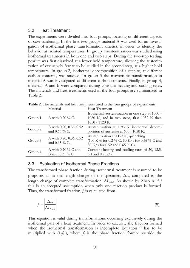
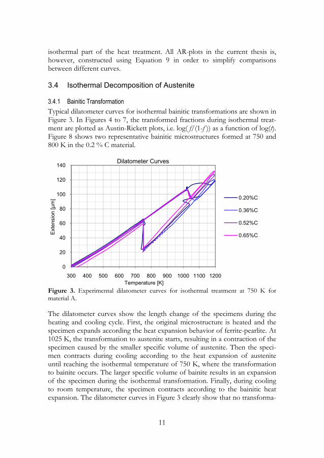
3.4.1 Bainitic Transformation Typical dilatometer curves for isothermal bainitic transformations are shown in Figure 3. In Figures 4 to 7, the transformed fractions during isothermal treat-ment are plotted as Austin-Rickett plots, i.e. log( f/(1-f )) as a function of log(t). Figure 8 shows two representative bainitic microstructures formed at 750 and 800 K in the 0.2 % C material.
Figure 3. Experimental dilatometer curves for isothermal treatment at 750 K for material A.
The dilatometer curves show the length change of the specimens during the heating and cooling cycle. First, the original microstructure is heated and the specimen expands according the heat expansion behavior of ferrite-pearlite. At 1025 K, the transformation to austenite starts, resulting in a contraction of the specimen caused by the smaller specific volume of austenite. Then the speci-men contracts during cooling according to the heat expansion of austenite until reaching the isothermal temperature of 750 K, where the transformation to bainite occurs. The larger specific volume of bainite results in an expansion of the specimen during the isothermal transformation. Finally, during cooling to room temperature, the specimen contracts according to the bainitic heat expansion. The dilatometer curves in Figure 3 clearly show that no transforma-
0
20
40
60
80
100
120
140
300 400 500 600 700 800 900 1000 1100 1200
Ext
ensi
on [µ
m]
Temperature [K]
Dilatometer Curves
0.20%C
0.36%C
0.52%C
0.65%C
12
tions occur during cooling after the isothermal transformation, revealing that all austenite is transformed during the isothermal treatment.
Figure 4. Austin-Rickett plots for the bainitic transformation at different temperatures for material A with 0.20 % C.
Figure 5. Austin-Rickett plots for the bainitic transformation at different temperatures for material A with 0.36 % C.
-1.5
-1
-0.5
0
0.5
1
1.5
-1 -0.5 0 0.5 1 1.5 2
log(
f/(1
-f ))
log(t)
AR-Plots for 0.20 % C
800K
750K
700K
650K
-1.5
-1
-0.5
0
0.5
1
1.5
0 0.5 1 1.5 2 2.5 3
log(
f/(1
-f))
log(t)
AR-Plots for 0.36 % C
800K
750K
700K
650K
13
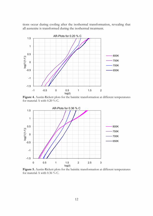
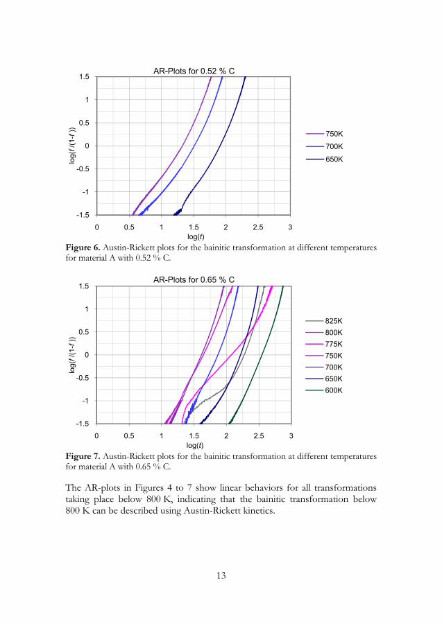
Figure 6. Austin-Rickett plots for the bainitic transformation at different temperatures for material A with 0.52 % C.
Figure 7. Austin-Rickett plots for the bainitic transformation at different temperatures for material A with 0.65 % C.
The AR-plots in Figures 4 to 7 show linear behaviors for all transformations taking place below 800 K, indicating that the bainitic transformation below 800 K can be described using Austin-Rickett kinetics.
-1.5
-1
-0.5
0
0.5
1
1.5
0 0.5 1 1.5 2 2.5 3
log(
f/(1
-f))
log(t)
AR-Plots for 0.52 % C
750K
700K
650K
-1.5
-1
-0.5
0
0.5
1
1.5
0 0.5 1 1.5 2 2.5 3
log(
f/(1
-f))
log(t)
AR-Plots for 0.65 % C
825K800K775K750K700K650K600K
14
a) 750 K.
b) 800 K.
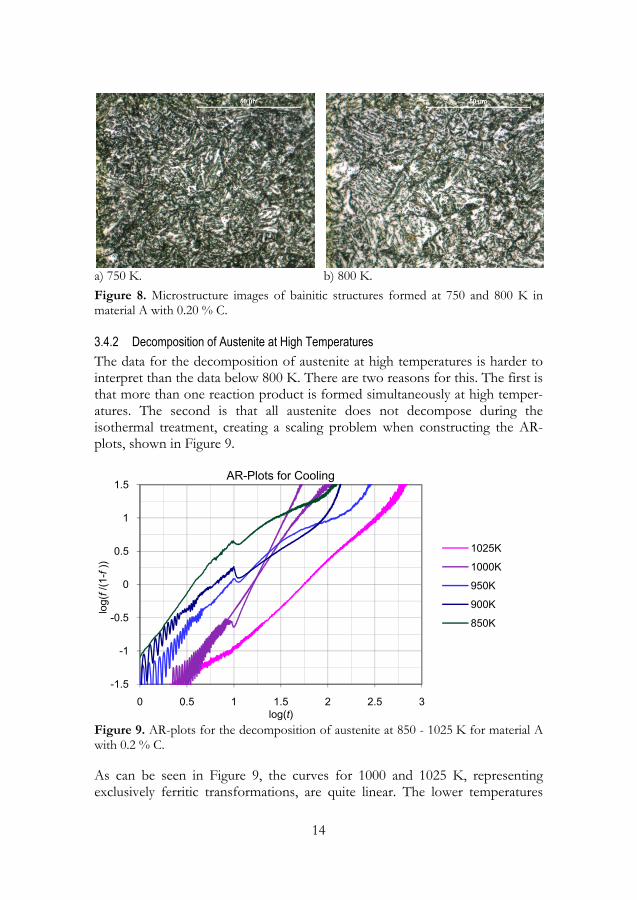
Figure 8. Microstructure images of bainitic structures formed at 750 and 800 K in material A with 0.20 % C.
3.4.2 Decomposition of Austenite at High Temperatures The data for the decomposition of austenite at high temperatures is harder to interpret than the data below 800 K. There are two reasons for this. The first is that more than one reaction product is formed simultaneously at high temper-atures. The second is that all austenite does not decompose during the isothermal treatment, creating a scaling problem when constructing the AR-plots, shown in Figure 9.
Figure 9. AR-plots for the decomposition of austenite at 850 - 1025 K for material A with 0.2 % C.
As can be seen in Figure 9, the curves for 1000 and 1025 K, representing exclusively ferritic transformations, are quite linear. The lower temperatures
-1.5
-1
-0.5
0
0.5
1
1.5
0 0.5 1 1.5 2 2.5 3
log(
f/(1
-f))
log(t)
AR-Plots for Cooling
1025K
1000K
950K
900K
850K
15
however, show non linear behaviors. At 900 and 950 K, ferrite and pearlite form simultaneously, and at 850 K bainite, ferrite and some pearlite form simultaneously. The linear nature of the ferritic curves indicates that the ferritic formation, like the bainitic formation, can be described using AR-kinetics and Equation 5. The parameters c and k for the ferritic transformation is however not yet evaluated.
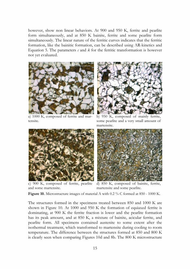
a) 1000 K, composed of ferrite and mar-tensite.
b) 950 K, composed of mainly ferrite, some pearlite and a very small amount of martensite.
c) 900 K, composed of ferrite, pearlite and some martensite.
d) 850 K, composed of bainite, ferrite, martensite and some pearlite.
Figure 10. Microstructure images of material A with 0.2 % C formed at 850 - 1000 K.
The structures formed in the specimens treated between 850 and 1000 K are shown in Figure 10. At 1000 and 950 K the formation of equiaxed ferrite is dominating, at 900 K the ferrite fraction is lower and the pearlite formation has its peak amount, and at 850 K, a mixture of bainite, acicular ferrite, and pearlite form. All specimens contained austenite to some extent after the isothermal treatment, which transformed to martensite during cooling to room temperature. The difference between the structures formed at 850 and 800 K is clearly seen when comparing Figures 10d and 8b. The 800 K microstructure
16
is almost entirely bainitic, while the 850 K microstructure is a mixture of bainite, acicular ferrite, martensite and some pearlite.
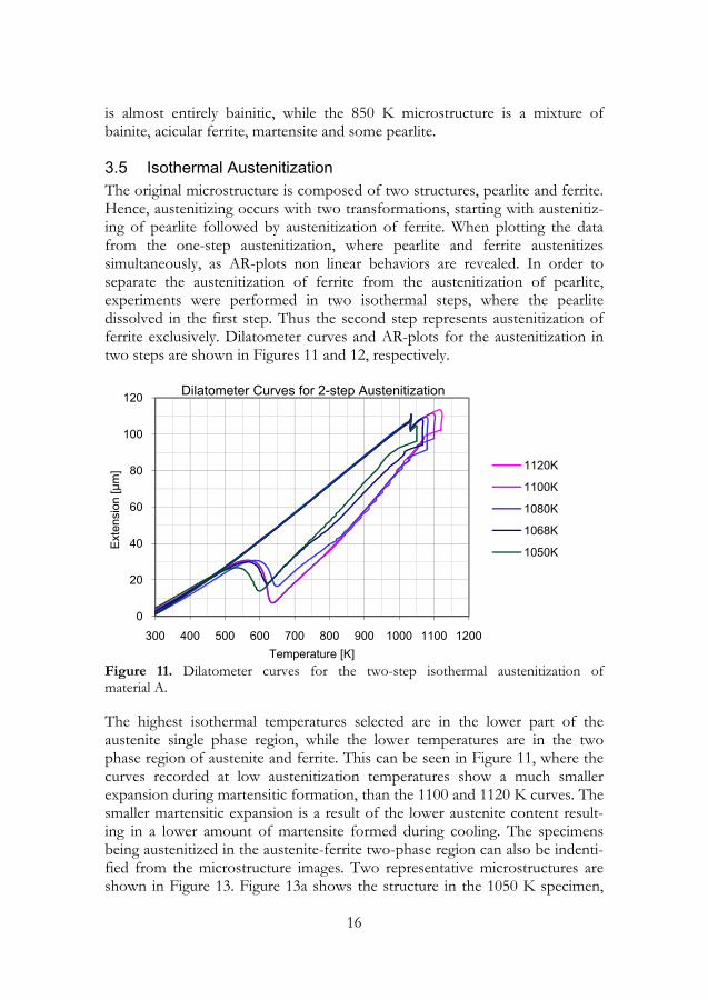
3.5 Isothermal Austenitization The original microstructure is composed of two structures, pearlite and ferrite. Hence, austenitizing occurs with two transformations, starting with austenitiz-ing of pearlite followed by austenitization of ferrite. When plotting the data from the one-step austenitization, where pearlite and ferrite austenitizes simultaneously, as AR-plots non linear behaviors are revealed. In order to separate the austenitization of ferrite from the austenitization of pearlite, experiments were performed in two isothermal steps, where the pearlite dissolved in the first step. Thus the second step represents austenitization of ferrite exclusively. Dilatometer curves and AR-plots for the austenitization in two steps are shown in Figures 11 and 12, respectively.
Figure 11. Dilatometer curves for the two-step isothermal austenitization of material A.
The highest isothermal temperatures selected are in the lower part of the austenite single phase region, while the lower temperatures are in the two phase region of austenite and ferrite. This can be seen in Figure 11, where the curves recorded at low austenitization temperatures show a much smaller expansion during martensitic formation, than the 1100 and 1120 K curves. The smaller martensitic expansion is a result of the lower austenite content result-ing in a lower amount of martensite formed during cooling. The specimens being austenitized in the austenite-ferrite two-phase region can also be indenti-fied from the microstructure images. Two representative microstructures are shown in Figure 13. Figure 13a shows the structure in the 1050 K specimen,
0
20
40
60
80
100
120
300 400 500 600 700 800 900 1000 1100 1200
Ext
ensi
on [µ
m]
Temperature [K]
Dilatometer Curves for 2-step Austenitization
1120K
1100K
1080K
1068K
1050K
17
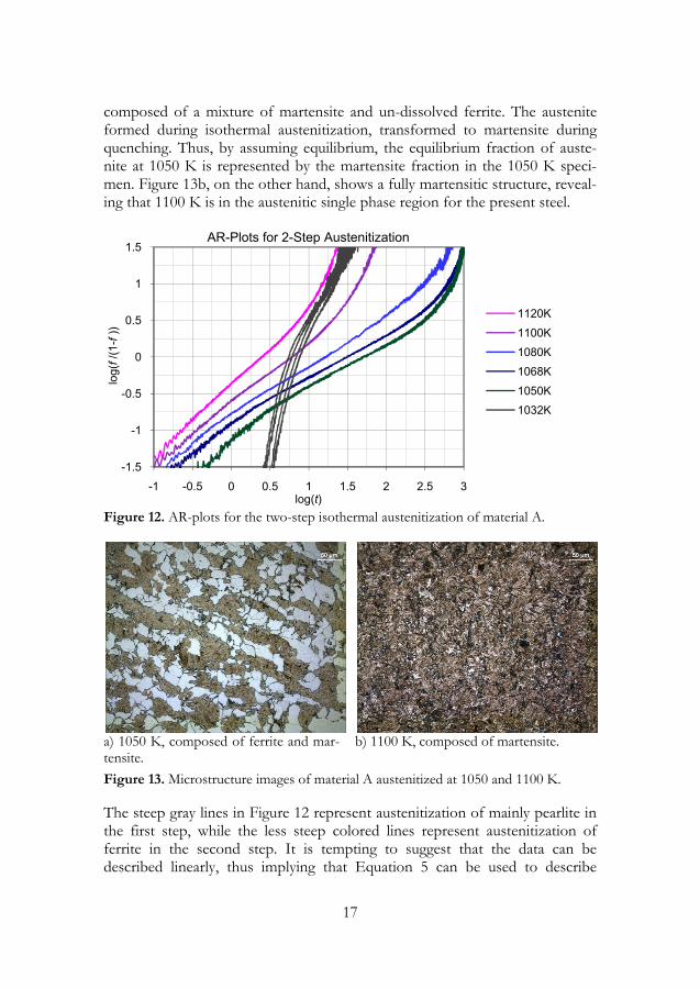
composed of a mixture of martensite and un-dissolved ferrite. The austenite formed during isothermal austenitization, transformed to martensite during quenching. Thus, by assuming equilibrium, the equilibrium fraction of auste-nite at 1050 K is represented by the martensite fraction in the 1050 K speci-men. Figure 13b, on the other hand, shows a fully martensitic structure, reveal-ing that 1100 K is in the austenitic single phase region for the present steel.
Figure 12. AR-plots for the two-step isothermal austenitization of material A.
a) 1050 K, composed of ferrite and mar-tensite.
b) 1100 K, composed of martensite.
Figure 13. Microstructure images of material A austenitized at 1050 and 1100 K.
The steep gray lines in Figure 12 represent austenitization of mainly pearlite in the first step, while the less steep colored lines represent austenitization of ferrite in the second step. It is tempting to suggest that the data can be described linearly, thus implying that Equation 5 can be used to describe
-1.5
-1
-0.5
0
0.5
1
1.5
-1 -0.5 0 0.5 1 1.5 2 2.5 3
log(
f/(1
-f))
log(t)
AR-Plots for 2-Step Austenitization
1120K1100K1080K1068K1050K1032K
18
austenitization of both pearlite and ferrite. The AR-parameters c and k for austenitization are however not yet evaluated.
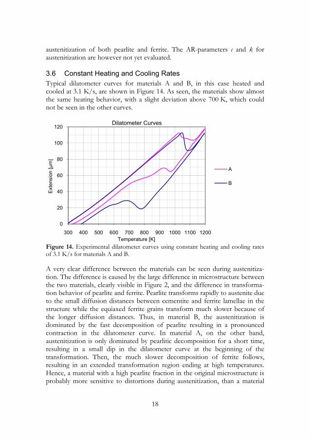
3.6 Constant Heating and Cooling Rates Typical dilatometer curves for materials A and B, in this case heated and cooled at 3.1 K/s, are shown in Figure 14. As seen, the materials show almost the same heating behavior, with a slight deviation above 700 K, which could not be seen in the other curves.
Figure 14. Experimental dilatometer curves using constant heating and cooling rates of 3.1 K/s for materials A and B.
A very clear difference between the materials can be seen during austenitiza-tion. The difference is caused by the large difference in microstructure between the two materials, clearly visible in Figure 2, and the difference in transforma-tion behavior of pearlite and ferrite. Pearlite transforms rapidly to austenite due to the small diffusion distances between cementite and ferrite lamellae in the structure while the equiaxed ferrite grains transform much slower because of the longer diffusion distances. Thus, in material B, the austenitization is dominated by the fast decomposition of pearlite resulting in a pronounced contraction in the dilatometer curve. In material A, on the other hand, austenitization is only dominated by pearlitic decomposition for a short time, resulting in a small dip in the dilatometer curve at the beginning of the transformation. Then, the much slower decomposition of ferrite follows, resulting in an extended transformation region ending at high temperatures. Hence, a material with a high pearlite fraction in the original microstructure is probably more sensitive to distortions during austenitization, than a material
0
20
40
60
80
100
120
300 400 500 600 700 800 900 1000 1100 1200
Ext
ensi
on [µ
m]
Temperature [K]
Dilatometer Curves
A
B
19
with a high ferrite fraction. Thus, it is more important to avoid non-uniform heating, during case hardening, when using a material with a large pearlite fraction in order to reduce distortions.
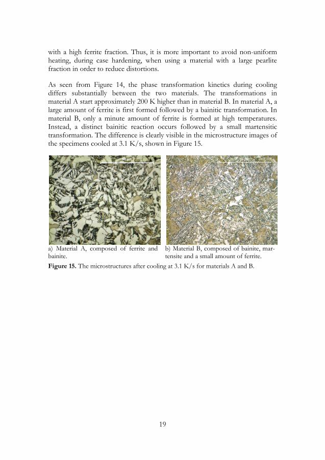
As seen from Figure 14, the phase transformation kinetics during cooling differs substantially between the two materials. The transformations in material A start approximately 200 K higher than in material B. In material A, a large amount of ferrite is first formed followed by a bainitic transformation. In material B, only a minute amount of ferrite is formed at high temperatures. Instead, a distinct bainitic reaction occurs followed by a small martensitic transformation. The difference is clearly visible in the microstructure images of the specimens cooled at 3.1 K/s, shown in Figure 15.
a) Material A, composed of ferrite and bainite.
b) Material B, composed of bainite, mar-tensite and a small amount of ferrite.
Figure 15. The microstructures after cooling at 3.1 K/s for materials A and B.

20
21
4 Evaluation of Model Parameters
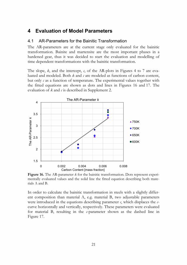
4.1 AR-Parameters for the Bainitic Transformation The AR-parameters are at the current stage only evaluated for the bainitic transformation. Bainite and martensite are the most important phases in a hardened gear, thus it was decided to start the evaluation and modelling of time dependent transformations with the bainitic transformation.
The slope, k, and the intercept, c, of the AR-plots in Figures 4 to 7 are eva-luated and modeled. Both k and c are modeled as functions of carbon content, but only c as a function of temperature. The experimental values together with the fitted equations are shown as dots and lines in Figures 16 and 17. The evaluation of k and c is described in Supplement 2.
Figure 16. The AR-parameter k for the bainitic transformation. Dots represent experi-mentally evaluated values and the solid line the fitted equation describing both mate-rials A and B.
In order to calculate the bainitic transformation in steels with a slightly differ-ent composition than material A, e.g. material B, two adjustable parameters were introduced in the equations describing parameter c, which displaces the c-curve horizontally and vertically, respectively. These parameters were evaluated for material B, resulting in the c-parameter shown as the dashed line in Figure 17.
1.5
2
2.5
3
3.5
4
0 0.002 0.004 0.006 0.008
The
AR
-Par
amet
er k
Carbon Content [mass fraction]
The AR-Parameter k
750K
700K
650K
600K
22
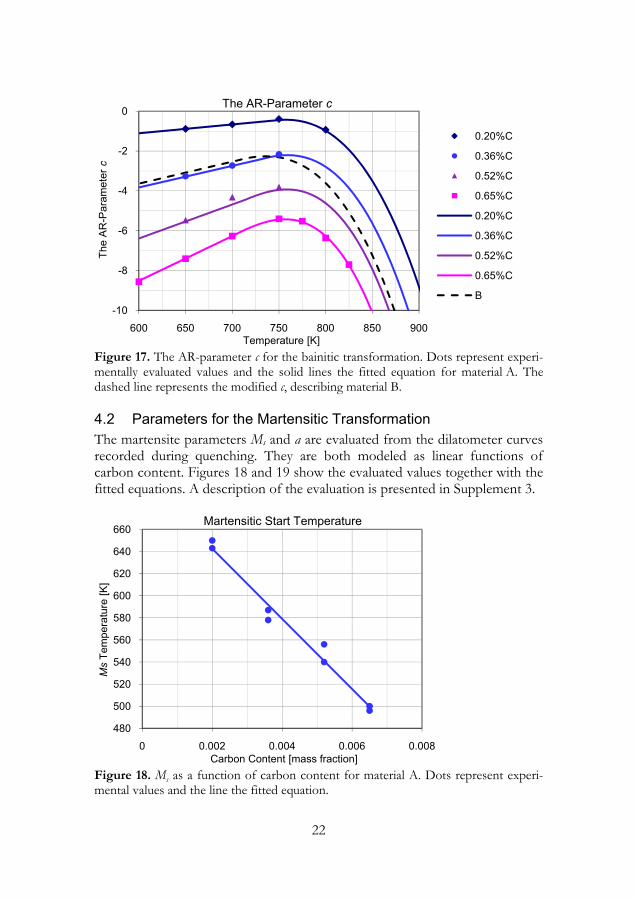
Figure 17. The AR-parameter c for the bainitic transformation. Dots represent experi-mentally evaluated values and the solid lines the fitted equation for material A. The dashed line represents the modified c, describing material B.
4.2 Parameters for the Martensitic Transformation The martensite parameters Ms and a are evaluated from the dilatometer curves recorded during quenching. They are both modeled as linear functions of carbon content. Figures 18 and 19 show the evaluated values together with the fitted equations. A description of the evaluation is presented in Supplement 3.
Figure 18. Ms as a function of carbon content for material A. Dots represent experi-mental values and the line the fitted equation.
-10
-8
-6
-4
-2
0
600 650 700 750 800 850 900
The
AR
-Par
amet
er c
Temperature [K]
The AR-Parameter c
0.20%C
0.36%C
0.52%C
0.65%C
0.20%C
0.36%C
0.52%C
0.65%C
B
480
500
520
540
560
580
600
620
640
660
0 0.002 0.004 0.006 0.008
Ms
Tem
pera
ture
[K]
Carbon Content [mass fraction]
Martensitic Start Temperature
23
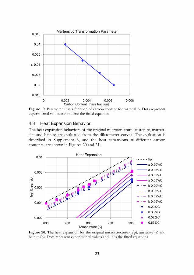
Figure 19. Parameter a, as a function of carbon content for material A. Dots represent experimental values and the line the fitted equation.
4.3 Heat Expansion Behavior The heat expansion behaviors of the original microstructure, austenite, marten-site and bainite are evaluated from the dilatometer curves. The evaluation is described in Supplement 3, and the heat expansions at different carbon contents, are shown in Figures 20 and 21.
Figure 20. The heat expansion for the original microstructure (f/p), austenite (a) and bainite (b). Dots represent experimental values and lines the fitted equations.
0.015
0.02
0.025
0.03
0.035
0.04
0.045
0 0.002 0.004 0.006 0.008
a
Carbon Content [mass fraction]
Martensitic Transformation Parameter
0.002
0.004
0.006
0.008
0.01
600 700 800 900 1000
Hea
t Exp
ansi
on
Temperature [K]
Heat Expansionf/pa 0.20%Ca 0.36%Ca 0.52%Ca 0.65%Cb 0.20%Cb 0.36%Cb 0.52%Cb 0.65%C0.20%C0.36%C0.52%C0.65%C
24
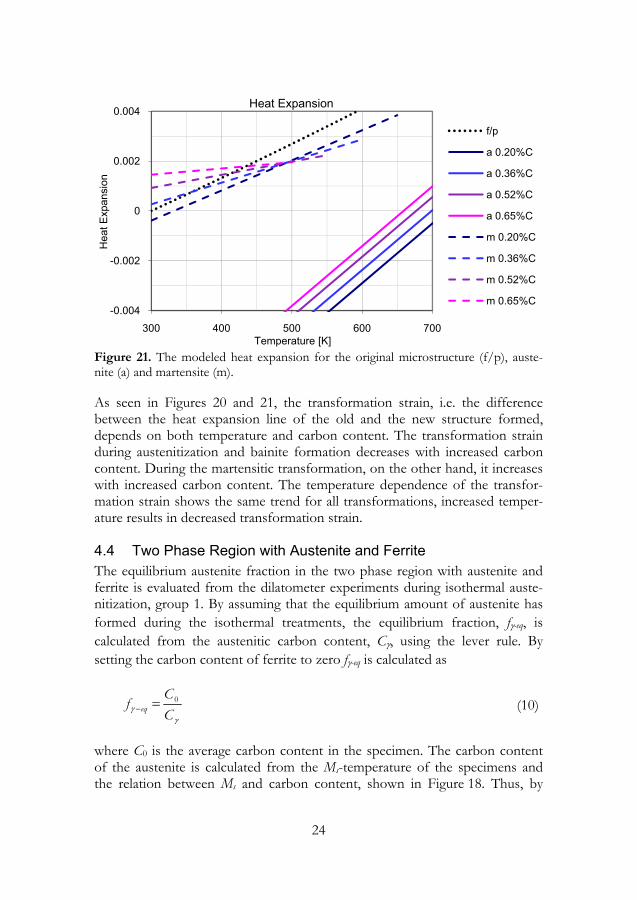
Figure 21. The modeled heat expansion for the original microstructure (f/p), auste-nite (a) and martensite (m).
As seen in Figures 20 and 21, the transformation strain, i.e. the difference between the heat expansion line of the old and the new structure formed, depends on both temperature and carbon content. The transformation strain during austenitization and bainite formation decreases with increased carbon content. During the martensitic transformation, on the other hand, it increases with increased carbon content. The temperature dependence of the transfor-mation strain shows the same trend for all transformations, increased temper-ature results in decreased transformation strain.
4.4 Two Phase Region with Austenite and Ferrite The equilibrium austenite fraction in the two phase region with austenite and ferrite is evaluated from the dilatometer experiments during isothermal auste-nitization, group 1. By assuming that the equilibrium amount of austenite has formed during the isothermal treatments, the equilibrium fraction, fγ-eq, is calculated from the austenitic carbon content, Cγ, using the lever rule. By setting the carbon content of ferrite to zero fγ-eq is calculated as
0eq
CfCγ
γ− = (10)
where C0 is the average carbon content in the specimen. The carbon content of the austenite is calculated from the Ms-temperature of the specimens and the relation between Ms and carbon content, shown in Figure 18. Thus, by
-0.004
-0.002
0
0.002
0.004
300 400 500 600 700
Hea
t Exp
ansi
on
Temperature [K]
Heat Expansion
f/p
a 0.20%C
a 0.36%C
a 0.52%C
a 0.65%C
m 0.20%C
m 0.36%C
m 0.52%C
m 0.65%C
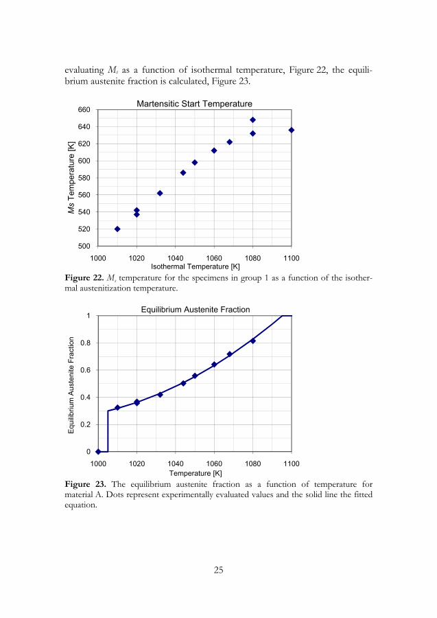
25
evaluating Ms as a function of isothermal temperature, Figure 22, the equili-brium austenite fraction is calculated, Figure 23.
Figure 22. Ms temperature for the specimens in group 1 as a function of the isother-mal austenitization temperature.
Figure 23. The equilibrium austenite fraction as a function of temperature for material A. Dots represent experimentally evaluated values and the solid line the fitted equation.
500
520
540
560
580
600
620
640
660
1000 1020 1040 1060 1080 1100
Ms
Tem
pera
ture
[K]
Isothermal Temperature [K]
Martensitic Start Temperature
0
0.2
0.4
0.6
0.8
1
1000 1020 1040 1060 1080 1100
Equ
ilibr
ium
Aus
teni
te F
ract
ion
Temperature [K]
Equilibrium Austenite Fraction

26
27
5 Results and Discussion
5.1 Isothermal Bainitic Transformation
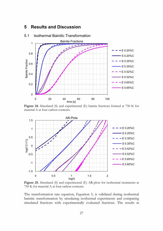
Figure 24. Simulated (S) and experimental (E) bainite fractions formed at 750 K for material A at four carbon contents.
Figure 25. Simulated (S) and experimental (E) AR-plots for isothermal treatments at 750 K for material A at four carbon contents.
The transformation rate equation, Equation 5, is validated during isothermal bainitic transformation by simulating isothermal experiments and comparing simulated fractions with experimentally evaluated fractions. The results at
0
0.2
0.4
0.6
0.8
1
0 20 40 60 80 100
Bai
nite
Fra
ctio
n
time [s]
Bainite Fractions
E 0.20%C
S 0.20%C
S 0.35%C
S 0.35%C
E 0.52%C
S 0.52%C
E 0.65%C
S 0.65%C
-1.5
-1
-0.5
0
0.5
1
1.5
0 0.5 1 1.5 2
log(
f/(1
-f))
log(t)
AR-Plots
E 0.20%C
S 0.20%C
E 0.35%C
S 0.35%C
E 0.52%C
S 0.52%C
E 0.65%C
S 0.65%C
28
750 K, representing the shortest transformation times, i.e. most important for industrial applications, are shown in Figures 24 and 25. As can be seen, the fit between the simulated and the experimentally evaluated bainite fractions is very good and quite adequate for simulation purposes.
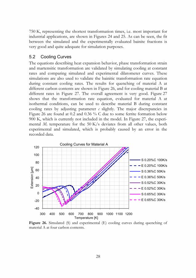
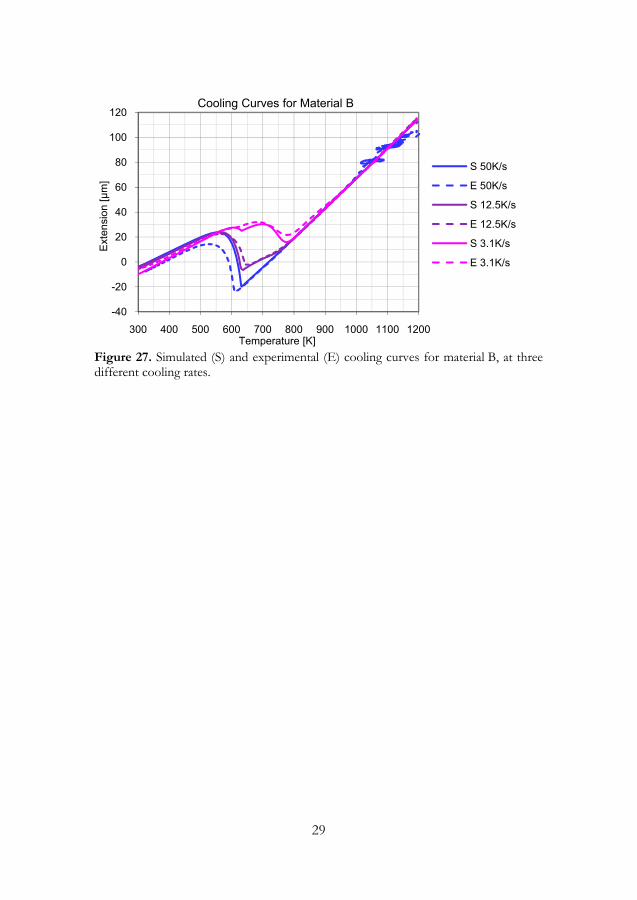
5.2 Cooling Curves The equations describing heat expansion behavior, phase transformation strain and martensitic transformation are validated by simulating cooling at constant rates and comparing simulated and experimental dilatometer curves. These simulations are also used to validate the bainitic transformation rate equation during constant cooling rates. The results for quenching of material A at different carbon contents are shown in Figure 26, and for cooling material B at different rates in Figure 27. The overall agreement is very good. Figure 27 shows that the transformation rate equation, evaluated for material A at isothermal conditions, can be used to describe material B during constant cooling rates by adjusting parameter c slightly. The major discrepancies in Figure 26 are found at 0.2 and 0.36 % C due to some ferrite formation below 900 K, which is currently not included in the model. In Figure 27, the experi-mental Ms temperature for the 50 K/s deviates from all other values, both experimental and simulated, which is probably caused by an error in the recorded data.
Figure 26. Simulated (S) and experimental (E) cooling curves during quenching of material A at four carbon contents.
-40
-20
0
20
40
60
80
100
120
300 400 500 600 700 800 900 1000 1100 1200
Ext
ensi
on [µ
m]
Temperature [K]
Cooling Curves for Material A
S 0.20%C 100K/s
E 0.20%C 100K/s
S 0.36%C 50K/s
E 0.36%C 50K/s
S 0.52%C 30K/s
E 0.52%C 30K/s
S 0.65%C 30K/s
E 0.65%C 30K/s
29
Figure 27. Simulated (S) and experimental (E) cooling curves for material B, at three different cooling rates.
-40
-20
0
20
40
60
80
100
120
300 400 500 600 700 800 900 1000 1100 1200
Ext
ensi
on [µ
m]
Temperature [K]
Cooling Curves for Material B
S 50K/s
E 50K/s
S 12.5K/s
E 12.5K/s
S 3.1K/s
E 3.1K/s

30
31
6 Conclusions • It is possible to rewrite the Austen-Rickett equation to a transformation
rate equation (Equation 5) independent of time. By time integration of the transformation rate, the bainite fraction was successfully calculated and compared to experimental data.
• By a simple adjustment of the c-parameter in the bainite transformation equation, a more alloyed material with considerably slower bainitic trans-formation kinetics can be described.
• The phase transformation strain is successfully described by assigning each phase an appropriate heat expansion and by describing the phase transfor-mations. When a transformation takes place, the transformation strain is automatically obtained as the material changes its heat expansion from the old phase mix to the heat expansion of the new mix.
• Transformation strain for ferrite-pearlite to austenite and for austenite to bainite transformations are reduced with increased carbon content and increased transformation temperature.
• The proportions of ferrite and pearlite in the original microstructure have a large effect on the volume change during austenitization, and can therefore affect the distortion in a hardened part. Since pearlite austenitizes much faster than ferrite, it is more important to control the heating during auste-nitization when using a material composed of mainly pearlite, than when using a material composed of mainly ferrite, in order to reduce distortions.
• From Supplement 2, it can be concluded that above 750 K the bainitic transformation in material A seems to start with a quick reaction forming a well organized microstructure followed by a slow reaction forming a less organized and coarser microstructure. The fraction formed by the quick reaction decreases linearly with increasing carbon content. At 0.65 % C the morphological difference between the 750 and 800 K specimens is pro-nounced whereas it is only minor at 0.20 % C.

32
33
7 Future Work In order to be able to calculate all important phase transformations occurring during case hardening, the AR-parameters for three additional transformations must be evaluated. These are austenitization of pearlite and ferrite and the transformation from austenite to ferrite. The austenitization of pearlite can be separated from the austenitization of ferrite by evaluating the pearlitic austeni-tization in specimens carburized to the eutectoid carbon content and heat treated to contain only pearlite.
For the model to be able to predict distortions, it must be able to calculate plastic deformation. Thus, the yield strength and the plastic behavior of the phases present must be evaluated as functions of temperature and carbon content. Then, when the model can describe plastic deformation occurring during hardening, it can be used to help optimize the manufacturing process. Important conditions can be altered in the model, in order to calculate the effects these factors have on distortion. Examples of such factors are non-uniform heating and cooling, non-uniform chemical composition and the amount of pearlite in the original microstructure. Hence, it will be possible to identify the factors being most important to control in order to reduce distor-tions.

34
35
Acknowledgements
First, I would like to thank my supervisor Stefan Jonsson, for the opportunity to do this work, and for all help and support during the work. I would also like to thank my family, especially my fiancé Fredrik Arnell, for supporting and helping me. Finally, I would like to thank my colleagues at KTH, for making this such a great place to work. A special thanks to Karin Mannesson, and also to Dennis Andersson for reading and commenting on the script.
Stockholm, October 2009
Matilda Tehler

36
37
References
1 H. Mallener, Harterei-Technische Mitteilungen, Mass- und Formänderung beim Einsatzhärten, 45 (1990) 1 pp. 66-72.
2 A. P. Gulyaev, Metal Science and Heat Treatment, Cold Treatment of Steel, 40 (1998) pp. 449-455.
3 S.-J. Lee, Y.-K. Lee, Materials Science Forum, Effect of Austenite Grain Size on Martensitic Transformation of a Low Alloy Steel, 475-479 (2005) pp. 3169-3172.
4 L.C.F. Canale, G.E. Totten, International Journal of Materials and Product Technology, Overview of distortion and residual stress due to quench processing part I: factors affecting quench distortion, 24 (2005) 1-4 pp. 4-52.
5 O. Kessler, H. Sturm, F. Hoffman, P, Mayr. Fourth international Conference on Quenching and Control of Distorsion, Influence of the Heating Parameters on the Distortion of Quench Hardened AISI 52100 Steel Bearing Rings, (2003) pp. 341-346.
6 H. Sturm, T. Karsch, O. Kessler, H-W. Zoch, Fifth international Conference on Quenching and Control of Distorsion, Out-of-roundness change of bearing rings due to non-uniform heating, (2007) pp. 233-240.
7 W. A. Johnson, R. F. Mehl, Trans. AIME, Reaction Kinetics in Processes of Nucleation and Grain Growth, 135 (1939) pp. 416-458.
8 M. Avrami, Journal of Chemical Physics, Kinetics of Phase Change. I, 7 (1939) pp. 1103-1112.
9 M. Avrami, Journal of Chemical Physics, Kinetics of Phase Change. II, 8 (1940) pp. 212-224.
10 A. N. Kolmorgorov, Izv. Akad. Nauk SSSR, 3 (1937) pp. 355-359.
11 J. B. Austin, R. I. Rickett, Trans. AIME, Kinetics of the Decomposition of Austenite at Constant Temperature, 135 (1939) pp. 397-415.
12 M. J. Starink, Journal of Materials Science, Kinetic Equations for Diffusion-Controlled Precipitation Reactions, 32 (1997) pp. 4061-4070.
13 D. P. Koistinen, R. E. Marburger, Acta Metallurgica, A general equation prescribing the extent of the austenite-martensite transformation in pure iron-carbon alloys and plain carbon steels, 7 (1959) pp. 59-60.
14 Home page of COMSOL Multiphysics, http://www.comsol.com/.
15 J. Z. Zhao, C. Mesplont, B. C. De Cooman, Materials Science and Engineering, Quantitative analysis of the dilatation during an isothermal decomposition of austenites, A332 (2002) pp. 110-116.