Surface Integral Equationsand the

Boundary Element Method

Homer Reid18.369 Guest Lecture

3/23/2012

Electromagnetic Scattering Problems

We have some known incident field (such as a plane wave), scattering fromsome known geometry (including objects of known shapes and materials)and we want to know the scattered fields. (Note: all quantities ∼ e−iωt.)

known known unknownHomer Reid: SIE/BEM Approach to Computational Electromagnetism 3/23/2012 2 / 16

Methods for Solving EM Scattering Problems, 1Expansions in special functions

Write the fields inside and outside the scatterer as expansions in sets of known Maxwell solutions(in some convenient coordinate system) and match coefficients.

Advantages:

• Exploits known Maxwell solutions=⇒ efficient

Disadvantages:

• Only works for a small number of geometries=⇒ not general.

One Sphere: “Mie scattering”

f(x) ∼ jl(r)Ylm(θ, φ)

Planar Slab: “Fresnel Coefficients”

f(x) ∼ eik·x

Homer Reid: SIE/BEM Approach to Computational Electromagnetism 3/23/2012 3 / 16

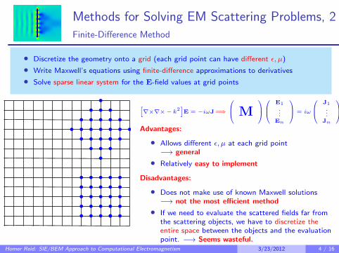
Methods for Solving EM Scattering Problems, 2Finite-Difference Method

• Discretize the geometry onto a grid (each grid point can have different ε, µ)

• Write Maxwell’s equations using finite-difference approximations to derivatives

• Solve sparse linear system for the E-field values at grid points

[∇×∇×− k2

]E = −iωJ=⇒

M

E1...

En

= iω

J1...

Jn

Advantages:

• Allows different ε, µ at each grid point−→ general

• Relatively easy to implement

Disadvantages:

• Does not make use of known Maxwell solutions−→ not the most efficient method

• If we need to evaluate the scattered fields far fromthe scattering objects, we have to discretize theentire space between the objects and the evaluationpoint. −→ Seems wasteful.

Homer Reid: SIE/BEM Approach to Computational Electromagnetism 3/23/2012 4 / 16

Methods for Solving EM Scattering Problems, 3Surface-Integral-Equation (SIE) Method

• First compute the surface current distribution K(x) induced by the incident field

• Then compute the scattered fields using K(x) and known Maxwell solutions:

Escat

(x) =

∮S

G(x− x′)K(x

′)dx

′ where G is the solution to[∇×∇× − k2

]G(r) = −iω1δ(r);

G (the “dyadic Green’s function”) is known in closed form

Advantages:

• Exploits known Maxwell solutions =⇒ efficient

• Allows scatterers of arbitrary shapes and arbitrary(homogeneous) materials =⇒ general

• Unknown quantities confined to object surfaces,not everywhere in space =⇒ not wasteful

Disadvantages:

• Difficult to implement

• Restricted to homogeneous scatterers, i.e.piecewise-constant ε, µ

Homer Reid: SIE/BEM Approach to Computational Electromagnetism 3/23/2012 5 / 16

SIE Formulation of Scattering ProblemsConsider a perfectly electrically conducting (PEC) scatterer in vacuum.

The incident field induces a surface electric current density K(x) on the object surface.

Surface current density K: units of currentlength

J(x‖, z)︸ ︷︷ ︸volume current

= K(x‖)︸ ︷︷ ︸surface current

· δ(z)

Once we know K(x), we can compute the scattered E−field anywhere we like:

Escat(x) =

∮SG(x− x′)K(x′)dx′

Gij(r) =eikr

4πk2r3

[1− ikr+(ikr)3

]δij +

[−3+3ikr− (ikr)2

]rirjr2

(r = |r|, k =

ω

c

)We determine K(x) by requiring that the total tangential E-field vanish at the object surface:

[Einc(x) + Escat(x)

]‖

= 0 =⇒∮SG‖(x,x

′)K(x′)dx′ = −Einc‖ (x)

(for points x on object surfaces) “electric field integral equation” (EFIE)

The EFIE is an integral equation for K(x) in terms of Einc.

Homer Reid: SIE/BEM Approach to Computational Electromagnetism 3/23/2012 6 / 16

Numerical Solution of SIEsThe boundary element method (BEM)

Given Einc(x), want to find K(x) that solves the EFIE:

∮SG‖(x,x

′)K(x′)dx′ = −Einc‖ (x)

Idea: (1) expand K(x) in some convenient set of N basis functions =⇒ N unknown coefficients

K(x) =N∑n=1

knfn(x),fn(x)

=

(tangential vector-valued basis functions

defined on the object surface

)

Idea: (2) test (inner-product) the EFIE with each basis function =⇒ N equations

⟨fm,

∮G · K︸︷︷︸∑

knfn

dA

⟩= −

⟨fm,E

inc

⟩=⇒

M k1

...kN

=

v1

...vN

N ×N linear system (“BEM system”)

Matrix elements: Mmn =⟨fm

∣∣∣G∣∣∣fn⟩ RHS vector: vm = −⟨fm

∣∣∣Einc⟩

Homer Reid: SIE/BEM Approach to Computational Electromagnetism 3/23/2012 7 / 16

Basis functions for SIE/BEM solversOne choice for compact 3D objects: “RWG basis functions”

Begin by discretizing (“meshing”) object surfaces into triangles:

Associate one basis function with each internal edge:

• These are “RWG basis functions” (named fortheir inventors: Rao, Wilton, Glisson)

• # of basis functions N ∝ # of triangles

• As we refine the discretization (shrink thetriangles), the discretization errors decrease,but the cost of solving the linear system growslike N3

Homer Reid: SIE/BEM Approach to Computational Electromagnetism 3/23/2012 8 / 16

Steps in a BEM Scattering CalculationFor a compact 3D scattering problem using RWG basis functions

1. Discretize object surfaces into triangles.

• A well-studied problem; high-quality free software packages are available.

2. Analyze the surface mesh and assign one basis function fn(x) to each interior edge.

• Some minor computational work; not too challenging.

3. Most difficult step: Assemble the BEM matrix M and RHS vector v.

Mmn =⟨fm

∣∣∣G∣∣∣fn⟩, vm = −⟨fm

∣∣∣Einc⟩

4. Solve the linear system Mk = v for the surface-current expansion coefficients kn.

• For N . 10, 000, use standard linear algebra software (lapack).

5. Use the surface current density K(x) =∑knfn(x) to compute the scattered fields.

Escat(x) =∑n

kn

∫GEE(x,x′)fn(x′)dx′, Hscat(x) =

∑n

kn

∫GME(x,x′)fn(x′)dx′,

where GEE is what we called “G” before and GME ∼ ∇×GEE.

Homer Reid: SIE/BEM Approach to Computational Electromagnetism 3/23/2012 9 / 16

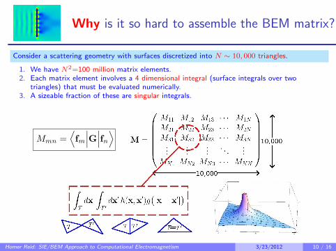
Why is it so hard to assemble the BEM matrix?

Consider a scattering geometry with surfaces discretized into N ∼ 10, 000 triangles.

1. We have N2=100 million matrix elements.2. Each matrix element involves a 4 dimensional integral (surface integrals over two

triangles) that must be evaluated numerically.3. A sizeable fraction of these are singular integrals.

Homer Reid: SIE/BEM Approach to Computational Electromagnetism 3/23/2012 10 / 16

SIE/BEM Techniques for Non-PEC GeometriesFor non-PEC geometries we must introduce effective magnetic surface currents

For PEC scatterers, the SIE/BEM procedure reflects a physical reality: the currents induced bythe incident field are confined to the object surface.

For general (non-PEC) scatterers, this is no longer true: the incident field induces currentsthroughout the volume of the scatterer.

Twooptions:

1. Volume integral equation: Write an integral equation for the volume electriccurrent distribution J(x) throughout the bulk of the scatterer.

2. Surface integral equation: Write an integral equation for effective electric andmagnetic surface currents K(x),N(x) on the surface of the scatterer.

PEC Non-PEC

Physics Surface electric current K Volume electric current J

Mathematics Surface electric current K Surface electric and magnetic currents K,N

Homer Reid: SIE/BEM Approach to Computational Electromagnetism 3/23/2012 12 / 16

Effective Surface Currents for non-PEC Geometries

The Stratton-Chu equations

Recall Green’s theorem: For a scalar field φ satisfying Laplace, knowledge of φ (or ∂φ∂n

) on theboundary ∂Ω of a closed source-free region Ω suffices to recover φ everywhere in the interior.

φ(x) =

∮∂Ω

G(x,x′)φ(x′)dA

The Stratton-Chu equations generalize Green’s theorem to the case of vector fields satifyingMaxwell: knowledge of tangential E, H on ∂Ω suffices to recover E and H throughout Ω.

E(x) =

∮∂Ω

GEE(x,x′)

[n×H(x′)

]+ GEM(x,x′)

[− n×E(x′)

]dA

H(x) =

∮∂Ω

GME(x,x′)

[n×H(x′)

]+ GMM(x,x′)

[− n×E(x′)

]dA

The source quantities that enter the Stratton-Chu equations are n×H and −n×E. Think ofthese as effective surface currents:

Keff(x) ≡ n×H, Neff(x) ≡ −n×E.

Homer Reid: SIE/BEM Approach to Computational Electromagnetism 3/23/2012 13 / 16

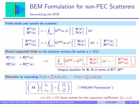
BEM Formulation for non-PEC ScatterersGeneralizing the EFIE

Fields inside and outside the scatterer:[Ein(x)Hin(x)

]= −

∮∂Ω

[Gin(x,x′)

] [K(x′)N(x′)

]dx′

[Eout(x)Hout(x)

]= +

∮∂Ω

[Gout(x,x′)

] [K(x′)N(x′)

]dx′ +

[Einc(x)Hinc(x)

]Match tangential fields at the scatterer surface (for points x ∈ ∂Ω):

Ein‖ (x) = Eout

‖ (x)

Hin‖ (x) = Hout

‖ (x)=⇒

∮∂Ω

[Gout + Gin

]‖

[K(x′)N(x′)

]dx′ = −

[Einc(x)Hinc(x)

]‖

Integral equation for K,N in terms of Einc,Hinc

Discretize by expanding K(x) =∑knfn(x), N(x) =

∑nnfn(x):(

M

)(kn

nn

)=

(vEn

vHn

)(”PMCHW Formulation”)

=⇒ 2N × 2N linear system for the expansion coefficients kn, nnHomer Reid: SIE/BEM Approach to Computational Electromagnetism 3/23/2012 14 / 16

scuff-em: An open-source BEM code suiteSurface-Current / Field Formulation of ElectroMagnetism

http://homerreid.com/scuff-EM

Features currently available:

• Scattering from compact 3D objects of arbitrary shapes• Arbitrary user-specified frequency-dependent ε, µ (isotropic, linear, piecewise constant)• Linux/Athena command-line interface to scattering code• C++ interface to scattering code• Application modules: Casimir forces, RF device modeling

Features coming soon:

• Python / Matlab interfaces to scattering codes• Scattering from periodic geometries

Homer Reid: SIE/BEM Approach to Computational Electromagnetism 3/23/2012 15 / 16

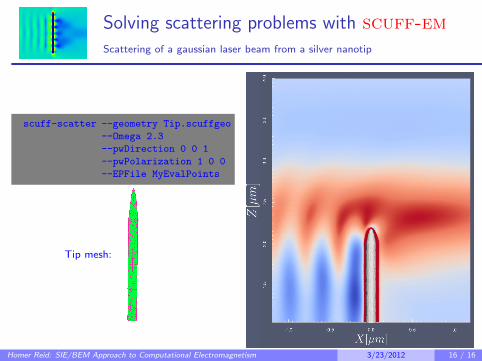
Solving scattering problems with scuff-emScattering of a gaussian laser beam from a silver nanotip

scuff-scatter --geometry Tip.scuffgeo

--Omega 2.3

--pwDirection 0 0 1

--pwPolarization 1 0 0

--EPFile MyEvalPoints

Tip mesh:

Homer Reid: SIE/BEM Approach to Computational Electromagnetism 3/23/2012 16 / 16