Matheus Alexandria Sposito Joao Basilio Pereima˜ matheus ...
56
SOLAR ENERGY DIFFUSION IN URBAN AREA: STRUCTURAL CHANGE AND COMPLEXITY Matheus Alexandria Sposito [email protected] Jo˜ ao Basilio Pereima [email protected] NeX-Nucleo of Economics and Complexity ECLAC - Summer School Santiago, Chile - 06/Ago/2019
Transcript of Matheus Alexandria Sposito Joao Basilio Pereima˜ matheus ...

SOLAR ENERGY DIFFUSION IN URBAN AREA:STRUCTURAL CHANGE AND COMPLEXITY
Matheus Alexandria [email protected]
Joao Basilio [email protected]
NeX-Nucleo of Economics and Complexity
ECLAC - Summer School
Santiago, Chile - 06/Ago/2019

Introduction Literature The Model Simulation Concluding Remarks References
THIS PRESENTATION
• Motivation• Literature• Model and Code• Results/simulations• Discussion
2 / 56

Introduction Literature The Model Simulation Concluding Remarks References
MOTIVATION
Cities are in the heart of challenging!
55% of global population livies in cities
65% of global energy demand
75% of global carbon dioxide emission
Source: REN21-Renewable Energy Policy Network for the 21st Century (2019). Renewables 2019 Global StatusReport, Paris: REN21 Secretariat, ISBN 978-3-9818911-7-1
3 / 56

Introduction Literature The Model Simulation Concluding Remarks References
MOTIVATION
FIGURE: Estimated Renewable Energy Share - 2017
Source: REN21-Renewable Energy Policy Network for the 21st Century (2019). Renewables 2019 Global Status Report,Paris: REN21 Secretariat, ISBN 978-3-9818911-7-1
4 / 56

Introduction Literature The Model Simulation Concluding Remarks References
MOTIVATION
FIGURE: Renewable Power Shares in Selected Cities, 2017
Source: REN21-Renewable Energy Policy Network for the 21st Century (2019). Renewables 2019 Global Status Report,Paris: REN21 Secretariat, ISBN 978-3-9818911-7-1
5 / 56

Introduction Literature The Model Simulation Concluding Remarks References
MOTIVATION
FIGURE: Overview of Existing 100% Renewable Energy Targets in Cities, 2018
Source: REN21-Renewable Energy Policy Network for the 21st Century (2019). Renewables 2019 Global Status Report,Paris: REN21 Secretariat, ISBN 978-3-9818911-7-1
6 / 56

Introduction Literature The Model Simulation Concluding Remarks References
MOTIVATION
FIGURE: The PV map: Brasil, Parana State and Europe
Fonte: Tiepolo, 20167 / 56

Introduction Literature The Model Simulation Concluding Remarks References
LITERATURE
• Total and Electrical Energy Demand and Efficiency:(REN21, 2019b,a)• Innovation Diffusion:
(Ryan and Gross, 1943; Rogers, 1962; Bass, 1969; Chow, 1967; Rogers, 2003)• Social Networks (Small World):
(Milgram, 1967; Travers and Milgram, 1969; Watts and Strogatz, 1998; Wasserman andFaust, 1994)• Interdependent Utility Function:
(Veblen, 1899; Granovetter, 1973, 1985; Mauss, 2003; Christakis and Fowler, 2009)• Consumer Behaviour - Understanding the path to purchase:
(Sproles and Kendall, 1986; Rogers, 2003; Shridhar, 2019)• Agent-based models:
(Dawid, 2006)• Agent-based models of decentralized solar power generation:
Zhao et al. (2011); Palmer et al. (2015); Robinson et al. (2013)
8 / 56

Introduction Literature The Model Simulation Concluding Remarks References
TOTAL AND ELECTRICAL ENERGY DEMAND AND EFFICIENCY
Efficiency and Conservation• In 2018, the IPCC presented several pathways for mitigating climate change and reduce
average temperature by 1.5o Celsius above pre-industrial levels.• The major recommendations are based at reducing global energy demand.• Reducing energy demand requires advances in both
• energy efficiency (technology-specific) and• energy conservation (behaviour-specific).
The three main determinants of total final energy demand• Sectoral structural changes within economies• Changes in the level of activity in each economic sector (economic growth)• Changes in the efficiency of energy use in each sector
9 / 56

Introduction Literature The Model Simulation Concluding Remarks References
ELECTRICITY CONSUMPTION
FIGURE: Average Electricity Consumption per Electrified Household, Selected Regions and World, 2012and 2017
Source: REN21-Renewable Energy Policy Network for the 21st Century (2019). Renewables 2019 Global Status Report,Paris: REN21 Secretariat, ISBN 978-3-9818911-7-1 10 / 56

Introduction Literature The Model Simulation Concluding Remarks References
INNOVATION DIFFUSION
Ryan and Gross (1943); Rogers (1962); Bass (1969); Chow (1967); Rogers (2003)
FIGURE: Bass Diffusion Curve
Source: Bass (1969)
11 / 56

Introduction Literature The Model Simulation Concluding Remarks References
CONSUMER BEHAVIOUR AND THE PATH TO PURCHASE
Type % Pop Female DictumImpulsive Spender 15% 55% “I love finding bargains”Conservative Homebody 13% 51% “Family matters most to me”Minimalist Seeker 12% 55% “I choose to focus o the simpler”Secure Traditionalist 12% 52% “I am content with where I am in life”Undaunted Striver 10% 56% “I want to have and be the best”Empowered Activist 9% 51% “I believe I have the power to affetc change”Inspired Adventurer 8% 53% “I strive to get more out of life”Digital Enthusiast 6% 54% “I incorporate technology in all areas of my life”Balanced Optimist 5% 51% “I am confident in myself and the future”Cautious Planner 4% 51% “I know what I want in life”
Source: EuroMonitor International, 2019. Survey Results: Using Consumer Types to Understand the Path toPurchase , Amrutha Shridhar, Research Consultant.
12 / 56

Introduction Literature The Model Simulation Concluding Remarks References
AGENT-BASED MODELS OF PV ENERGY
• Zhao et al. (2011) (USA)• Palmer et al. (2015) (Italia)• Robinson et al. (2013) (USA)
13 / 56

Introduction Literature The Model Simulation Concluding Remarks References
THE MODEL - SHORT DESCRIPTION
Dynamics• Temporal dynamics: hourly, monthly and annual accounting• Spacial dynamics: diffusion by residence and neighbourhood within a city• Climatic layer: solar radiation by hourly and monthly average• Electrical network IEE 33 bar system• Social Network tying heterogeneous households•
14 / 56

Introduction Literature The Model Simulation Concluding Remarks References
ALGORITHMS
• Netlogo for main algorithm• Matlab and Newton-Raphson method for stabilize the electrical network (Eltamaly et al.,
2018)• R for analysis
15 / 56

Introduction Literature The Model Simulation Concluding Remarks References
THE TIMELINE
The timeline consider hourly computation of consumed and produced energy.1 day - 24 hours1 month - 30 x 1 representative day (all days are equal within a month)Total computation = 24 x 120 = 2880 steps (ot ticks in Netlogo language)
FIGURE: Hourly, monthly and annual computation
16 / 56

Introduction Literature The Model Simulation Concluding Remarks References
URBAN TOPOLOGY
1 32 neighbourhood
2 120 residences in each neighbourhood
3 3840 residences in total
4 1 electrical node (transformer) in each neighbourhood
17 / 56

Introduction Literature The Model Simulation Concluding Remarks References
THE CITY
FIGURE: Hypotetical Topology - actual version
18 / 56

Introduction Literature The Model Simulation Concluding Remarks References
CLIMATE
The PV panel production depends on the temperature and radiation:
Th,t = Th,t + e1h,t onde e1
h,tN ∼ (0, σ1h,t) (1)
Rh,t = Rh,t + e2h,t onde e2
h,tN ∼ (0, σ2h,t) (2)
where h = 1, .., 24 is the hour of a day and t = 1, ..., 12 is the month.
19 / 56

Introduction Literature The Model Simulation Concluding Remarks References
IRRADIATION MAP
FIGURE: 5 year average, Curitiba, Brazil
20 / 56

Introduction Literature The Model Simulation Concluding Remarks References
ELECTRIC NETWORK
IEEE 33 bar system:
FIGURE: IEEE 33 Barras
An adjacent matrix can be easily set to representany real case.
0 1 0 0 ...0 1 0 0 ...0 0 1 1 ...0 0 0 1 ......
......
...
21 / 56

Introduction Literature The Model Simulation Concluding Remarks References
PRICE AND TARIFFS
It’s commom to use Feed-in tariffs for solar energy sellers.
Feed-in tariffs (FIT) are fixed electricity prices that are paid to renewable energy (RE)producers for each unit of energy produced and injected into the electricity grid. The paymentof the FIT is guaranteed for a certain period of time that is often related to the economic lifetimeof the respective RE project (usually between 15-25 years). Another possibility is to calculate afixed maximum amount of full-load hours of RE electricity production for which the FIT will bepaid. FIT are usually paid by electricity grid, system or market operators, often in the context ofPower purchasing agreements (PPA).
Source: https://energypedia.info/wiki/Feed-in_Tariffs_(FIT)
22 / 56

Introduction Literature The Model Simulation Concluding Remarks References
SALE PRICE
Two prices: for buying and selling energy.
PGi,h,t = β1 + β2PCi,h,t (3)
G - for “generated” energy set in kWhC - for “consumption”
When β1 = 0 and β2 = 1,
PGi,h,t = PCi,h,t (Brazilian case currently)
23 / 56

Introduction Literature The Model Simulation Concluding Remarks References
CONSUMPTION PRICE
The price paid by a household before taxes is set by computing the following equation:
PCi,h,t = PCi,h,0(Yi, Cmesi , S)[
1− β0
(F tecano−1
F
)](4)
TABLE: Energy Price in Brazil, Parana, kWh
Tariff Regime (S) R$/kWh[1]
Commom Tariff (S = 1)Baseline Tariff 0,50752Low Income[2]-Consumption ≤30 kWh 0,16188Low Income-Consumption between 31 kWh e 100 kWh 0,27750Low Income-Consumption between 101 kWh e 220 kWh 0,41625Low Income-Consumption geq 220 kWh 0,46250Brazilian White Tariff (S = 2)[3]
From 18h00 to 21h00 0,91974From 17h00 to 18h00 and 21h00 to 22h00 0,59690From 22h00 to 17h00 0,43568Source: Built using data from COPEL, 2019(1) Price without consumer taxes.(2) Low income households less than 3 minimum wage(3) Tariff set hourly.
24 / 56
Introduction Literature The Model Simulation Concluding Remarks References
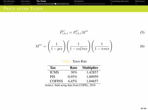
PRICE AFTER TAXES
PCi,h,t = PCi,h,tMtr (5)
M tr =
(1
1− pis
)(1
1− cofins
)(1
1− icms
)(6)
TABLE: Taxes Rate
Tax Rate MultiplierICMS 30% 1,42857PIS 0,95% 1,00959COFINS 4,45% 1,04657
Source: built using data from COPEL, 2019.
25 / 56

Introduction Literature The Model Simulation Concluding Remarks References
DAILY CONSUMPTION PATTERN
The consumption pattern of a Brazilian household depends on the income level Francisquini(2006).
FIGURE: Average charge of a household whoconsume less than 100 kWh/month
Source: Adapted from Francisquini (2006).
FIGURE: Average charge of a household whoconsume between 101 and 200 kWh/month
Source: Adapted from Francisquini (2006).
26 / 56

Introduction Literature The Model Simulation Concluding Remarks References
DAILY CONSUMPTION PATTERN
FIGURE: Average charge of a household whoconsume between 201 e 300 kWh/mes
Source: Adapted from Francisquini (2006).
FIGURE: Average charge of a household whoconsume between 301 a 500 kWh/mes
Source: Adapted from Francisquini (2006).
27 / 56

Introduction Literature The Model Simulation Concluding Remarks References
DAILY CONSUMPTION PATTERN
FIGURE: Average charge of a household who consume between 500 que kWh/mes
Source: Adapted from Francisquini (2006).
28 / 56

Introduction Literature The Model Simulation Concluding Remarks References
INCOME LEVEL AND DISTRIBUTION
TABLE: Household income level
Income Class- R$ Class≥ 18.740 A9.370 - 18.740 B3.748 - 9.370 C1.874 - 3.748 D0 - 1.874 E
Source: IBGE-Brazilian Institute of Geography and Statistics.
29 / 56

Introduction Literature The Model Simulation Concluding Remarks References
INVESTIMENT BY HOUSEHOLDS: HOW MUCH POWER TO CREATE
Based on Brazilian rules (ANEEL no 482/2012):• Micro producers can not have financial return by selling energy• The value of production must be monthly compensated by the value of consumption• If eventually production is higher then consumption, a household can accumulate credit for
next 12 months
The monetary amount of new capital adopted by a household i in month t (Ki,t) is:
Ki,t =12∑24
h=1
(Ch,i,tP
Gi,t
)∑12t=1
∑24h=1
(Ωh,tPGi,h,t
) (7)
where:
Ωh,t = Rh,t1000W [1− 0, 0045(Th,t + 15)] (8)
Trick theory: the consumer becomes also a producer!
30 / 56

Introduction Literature The Model Simulation Concluding Remarks References
INVESTIMENT BY HOUSEHOLDS: HOW MUCH POWER TO CREATE
Based on Brazilian rules (ANEEL no 482/2012):• Micro producers can not have financial return by selling energy (Amazing rule!!)• The value of production must be monthly compensated by the value of consumption• If eventually production is higher then consumption, a household can accumulate credit for
next 12 months
The monetary amount of new capital adopted by a household i in month t (Ki,t) is:
Ki,t =12∑24
h=1
(Ch,i,tP
Gi,t
)∑12t=1
∑24h=1
(Ωh,tPGi,h,t
) (9)
where:
Ωh,t = Rh,t1000W [1− 0, 0045(Th,t + 15)] (10)
Trick theory: the consumer becomes also a producer!
31 / 56

Introduction Literature The Model Simulation Concluding Remarks References
INVESTMENT BY HOUSEHOLDS: HOW MUCH POWER TO CREATE
Each month a household take into account a bunch of internal and external factors (variables):
Di,t = α1F1(ROIi,t) + α2F2(Linksi,t) + α3F3(Yi) + α4F4(Profilei) (11)
where Dt,i is linear combination of other four functions which depends on the both: ROI ,return of investment rate, social network (Links), income (Y ) and individual profile towardstechnology (Profile), following Rogers (2003) typology. The parameters α1...4 represents theweight of each function. The functions F1...4 and its functional form will be defined later.
32 / 56

Introduction Literature The Model Simulation Concluding Remarks References
INVESTIMENT BY HOUSEHOLDS: HOW MUCH POWER TO CREATE
The probability of a household adopt a PV plant and became a producer is, therefore:
P (D)i,t = 2
1 + e−θ0D
θ1i,t
− 1 (12)
which follow a logistic curve. Parameters θ0 and θ1 can be set to shape de S curve.Such probability is then compared to a uniform random number U1
i,t
f(n)i,t =
0, se P (e)i,t ≤ U1m,i
1, se P (e)i,t > U1m,i
(13)
and
Kei,t = f(n)i,tKi,t (14)
where, Kei,t is the effective installed capacity of household i in time t.
The installed capacity cost (investment) is:
PKi,t = (1− φ)(β3 + β4Kei,t) (15)
where φ is a subsidy rate and β3 and β4 are price parameters of PV panels in kWh.
33 / 56

Introduction Literature The Model Simulation Concluding Remarks References
BASELINE PARAMETERS
TABLE: Parameters of the baseline simulation
Description Parameters ValuesSize of the City 88×44Number of households F 3840Number of neighbourhoods N 32Parameters for buying price β0 0.70Weight of ROI α1 0,175Weight of Social links α2 0.400Weight of income α3 0.150Weight of Consumer Profile α4 0.150Social Network Density γ1,2 0.40, 3.0Parameter of Logistic Curve and ROI γ3,4,5 15, 2, 0.05Tariff Regime S Common (1)Subsidy φ 0Parameters for sale price β1,2 0/1Price of PV panels β3,4 4256,09/4537,69Interest Rate r 0,05Households Profile Rogers
34 / 56

Introduction Literature The Model Simulation Concluding Remarks References
BASELINE PARAMETERS
TABLE: Neighbourhood, Income Distribution and Electric Network
Neighbourhood Social Class IEEE 33 bar01/02/03/04 A 02/02/04/0505/06/07/08 B 06/07/08/0909/10/11/12 C 10/11/12/1313/14/15/16 C 14/15/16/1717/18/19/20 C 18/19/20/2121/22/23/24 C 22/23/24/2525/26/27/28 D 26/27/28/2929/20/31/32 E 30/31/32/33
35 / 56

Introduction Literature The Model Simulation Concluding Remarks References
SIMULATION RESULTS
All the result are average values of 100 simulations.
FIGURE: Number of Adopters FIGURE: Adopters by Social Class
36 / 56

Introduction Literature The Model Simulation Concluding Remarks References
SIMULATION RESULTS
FIGURE: Installed Capacity FIGURE: Charge and Production
37 / 56

Introduction Literature The Model Simulation Concluding Remarks References
SIMULATION RESULTS
FIGURE: Charge and Production at a representative day
38 / 56

Introduction Literature The Model Simulation Concluding Remarks References
SIMULATION RESULTS
FIGURE: Total Maximum System Voltage FIGURE: Total Minimum System Voltage
FIGURE: Waste Power
39 / 56

Introduction Literature The Model Simulation Concluding Remarks References
SOME SENSIBILITY ANALYSIS
FIGURE: Average Effect of Social Links - Social Network Density
40 / 56

Introduction Literature The Model Simulation Concluding Remarks References
SOME SENSIBILITY ANALYSIS
FIGURE: Percent of Adopters by Social Network Density (Social Links)
FIGURE: Installed Capacity by Social NetworkDensity (Social Links)
FIGURE: Total Investment by Social Network Density(Social Links)
41 / 56

Introduction Literature The Model Simulation Concluding Remarks References
SOME SENSIBILITY ANALYSIS
TABLE: Different Behaviour/Profiles
Society Profile IN[1] EA[2] EM[3] LM[4] LG[5]
Rogers 2,5% 13,5% 34% 34% 16%Innovative 25% 30% 25% 15% 5%Neutral 10% 25% 30% 25% 10%Conservative 5% 15% 25% 30% 25%Homogeneous 20% 20% 20% 20% 20%
(1) Innovators(2) Early Adopters
(3) Early Majority(4) Late Majority(5) Laggards
FIGURE: Percent of Adopters to Different Profiles
42 / 56

Introduction Literature The Model Simulation Concluding Remarks References
SOME SENSIBILITY ANALYSIS
FIGURE: The effect of β0 in the final number ofadopters
FIGURE: The effect of β0 in the Installed Capacity
43 / 56

Introduction Literature The Model Simulation Concluding Remarks References
SOME SENSIBILITY ANALYSIS
TABLE: Income Distribution and Electric Network by Neighbourhood
Neighbourhood Social Class IEEE33 bars01/02/03/04 A 18/22/33/2505/06/07/08 B 17/21/32/2409/10/11/12 C 10/11/12/1313/14/15/16 C 14/15/16/0617/18/19/20 C 02/19/20/0721/22/23/24 C 03/23/09/0525/26/27/28 D 26/27/28/2929/20/31/32 E 30/31/08/04
44 / 56

Introduction Literature The Model Simulation Concluding Remarks References
SOME SENSIBILITY ANALYSIS
FIGURE: Total Maximum Voltage in theReconfigured System
FIGURE: Total Minimum Voltage in the ReconfiguredSystem
FIGURE: Waste in the Reconfigured System
45 / 56

Introduction Literature The Model Simulation Concluding Remarks References
SOME SENSIBILITY ANALYSIS
FIGURE: Percent of Adopters by Interest Rate FIGURE: Final Adopters by Interest Rate
FIGURE: Final Adopters, Class A, by Interest Rate FIGURE: Final Adopters, Class B, by Interest Rate
46 / 56

Introduction Literature The Model Simulation Concluding Remarks References
SOME SENSIBILITY ANALYSIS
FIGURE: Final Adopters, Class C by Interest Rate
FIGURE: Final Adopters, Class D by Interest Rate
FIGURE: Final Adopters, Class D by Interest Rate
47 / 56

Introduction Literature The Model Simulation Concluding Remarks References
SOME SENSIBILITY ANALYSIS
FIGURE: Percent of Adopters by ICMS Tax Rate(over consumption) FIGURE: Final Adopters by ICMS Tax Rate
48 / 56

Introduction Literature The Model Simulation Concluding Remarks References
SOME SENSIBILITY ANALYSIS
FIGURE: Percent of Adopters by Subsidy Rate FIGURE: Final Adopters by Subsidy Rate
FIGURE: Final Adopters, Classe A by Subsidy Rate FIGURE: Final Adopters, Classe B by Subsidy Rate
49 / 56

Introduction Literature The Model Simulation Concluding Remarks References
SOME SENSIBILITY ANALYSIS
FIGURE: Final Adopters, Classe C by Subsidy Rate FIGURE: Final Adopters, Classe D by Subsidy Rate
FIGURE: Final Adopters, Classe D by Subsidy Rate
50 / 56
Introduction Literature The Model Simulation Concluding Remarks References
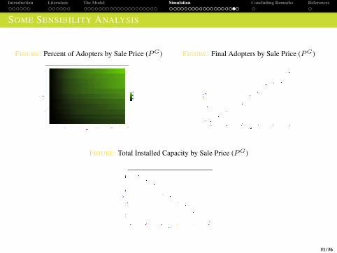
SOME SENSIBILITY ANALYSIS
FIGURE: Percent of Adopters by Sale Price (PG) FIGURE: Final Adopters by Sale Price (PG)
FIGURE: Total Installed Capacity by Sale Price (PG)
51 / 56

Introduction Literature The Model Simulation Concluding Remarks References
SOME SENSIBILITY ANALYSIS
FIGURE: Percent of Adopters by Power Tariff (Price for buying)
FIGURE: Installed Capacity by Power Tariff (Pricefor buying)
FIGURE: Household Investment by Power Tariff(Price for buying)
52 / 56

Introduction Literature The Model Simulation Concluding Remarks References
CONCLUDING REMARKS
• Class A and B will be the only benefited in the current Brazilian framework. It is anincome concentrator model• Cities can be self sufficient during the day, even surplus, for residential consumption• Decentralized power generation can be a drive for reducing demand over fossil fuels• This is a basic model, which can be expanded in many directions:
• Inter-temporal credit mechanism to household• Analyse the effect of free market to sell unlimited amount of energy• Use real topology of Cities• Connect decentralised urban generation with total market of energy• Build a national network of self sufficient cities connecting then in a pool of cities evolving at
the same time, even at different stage• Include labour market dynamics considering manufacturer and installers• Include endogenous technological change• Connect it with electric cars diffusion (new demand pattern)• Include new storage technology which can make the system more efficient• Explore the complexity of such system by using more encompassing agent-based model
This is a challenging and large research program.We know how to conduct it, but we need resources
53 / 56

Introduction Literature The Model Simulation Concluding Remarks References
REFERENCIAS I
Bass, F. M. (1969). A new product growth for model consumer durables. Management science,15(5):215–227.
Chow, G. C. (1967). Technological change and the demand for computers. The American EconomicReview, pages 1117–1130.
Christakis, N. A. and Fowler, J. H. (2009). Connected: The surprising power of our social networks andhow they shape our lives. Little, Brown.
Dawid, H. (2006). Agent-based models of innovation and technological change. In Tesfatsion, L. and Judd,K., editors, Handbook of Computational Economics, pages 1235–1272 (chapter 25). North-Holland,Amsterdam, The Netherlands.
Eltamaly, A. M., Sayed, Y., El-Sayed, A.-H., and Elghaffar, A. N. A. (2018). Optimum power flow analysisby newton raphson method, a case study. In ANNALS of Faculty Engineering Hunedoara, InternationalJournal of Engineering. Tome XVI, Fascicule 4, November.
Francisquini, A. A. (2006). Estimacao de Curvas de Carga em Pontos de Consumo e em Transformadoresde Distribuicao. PhD thesis, Universidade Estadual Paulista (UNESP).
Granovetter, M. (1985). Economic action and social structure: The problem of embeddedness. Americanjournal of sociology, 91(3):481–510.
Granovetter, M. S. (1973). The strength of weak ties. American Journal of Sociology, 78(6):1360–1380.
Mauss, M. (2003). Ensaio sobre a dadiva, forma e razao da troca nas sociedades arcaicas. Sociologıa eantropologıa.
Milgram, S. (1967). The small-world problem. Psychology Today, 1(1).
54 / 56

Introduction Literature The Model Simulation Concluding Remarks References
REFERENCIAS II
Palmer, J., Sorda, G., and Madlener, R. (2015). Modeling the diffusion of residential photovoltaic systemsin italy: An agent-based simulation. Technological Forecasting and Social Change, 99:106–131.
REN21 (2019a). Renewables 2019: Global status report.REN21 (2019b). Renewables in cities:2019 global status report.Robinson, S. A., Stringer, M., Rai, V., and Tondon, A. (2013). Gis-integrated agent-based model of
residential solar pv diffusion. In 32nd USAEE/IAEE North American Conference, pages 28–31.Rogers, E. M. (1962). The diffusion of innovations. 1th edition.Rogers, E. M. (2003). The diffusion of innovation. New York: Free Press, 5 edition.Ryan, B. and Gross, N. C. (1943). The diffusion of hybrid seed corn in two iowa communities. Rural
Sociology, 8(1):15–25.Shridhar, A. (2019). Using consumer types to understand the path to purchase.Sproles, G. B. and Kendall, E. L. (1986). A methodology for profiling consumers’ decision-marking styles.
Journal of Consumer Affairs, 20(2):267–279.Travers, J. and Milgram, S. (1969). An experimental study of the small world problem. Sociometry,
32(4):425–443.Veblen, T. (1899). The Theory of the Leisure Class: An Economic Study of Institutions. The Modern
Library, New York. printed 1934.Wasserman, S. and Faust, K. (1994). Social network analysis: Methods and applications, volume 8.
Cambridge university press.Watts, D. J. and Strogatz, S. H. (1998). Collective dynamics of small-world networks. Nature,
393(6684):440.Zhao, J., Mazhari, E., Celik, N., and Son, Y.-J. (2011). Hybrid agent-based simulation for policy evaluation
of solar power generation systems. Simulation Modelling Practice and Theory, 19(10):2189–2205.55 / 56

Introduction Literature The Model Simulation Concluding Remarks References
Thank you!
NeX-Nucleo of Economics and Complexity
Complex science for a better World
56 / 56