MATHEMATICS-II - Institute Of Aeronautical Engineering PPT(16-17).pdf · TEXT BOOKS Advanced...
118
MATHEMATICS-II Prepared by : Ms. P. Rajani , Asstistant Professor, Freshman Engineering
Transcript of MATHEMATICS-II - Institute Of Aeronautical Engineering PPT(16-17).pdf · TEXT BOOKS Advanced...
MATHEMATICS-II
Prepared by : Ms. P. Rajani , Asstistant Professor, Freshman Engineering

CONTENTS UNIT-I:Vector Calculus
UNIT-II: Fourier series and Fourier transforms
UNIT-III: Interpolation and Curve Fitting
UNIT-IV: Solutions of Algebraic and transcendental equations and Linear system of equations
UNIT-V: Numerical Integration and Numerical solutions of First order differential equations

TEXT BOOKS
Advanced Engineering Mathematics by Kreyszig, John Wiley & Sons.
Higher Engineering Mathematics by Dr. B.S. Grewal, Khanna Publishers
REFERENCES Mathematical Methods by T.K.V. Iyengar,
B.Krishna Gandhi & Others, S. Chand.
Introductory Methods by Numerical Analysis by S.S. Sastry, PHI Learning Pvt. Ltd.
Mathematical Methods by G.ShankarRao, I.K. International Publications, N.Delhi
Mathematical Methods by V. Ravindranath, Etl, Himalaya Publications.

REFERENCES Advanced Engineering Mathematics with
MATLAB, Dean G. Duffy, 3rd Edi, 2013, CRC Press Taylor & Francis Group.
6. Mathematics for Engineers and Scientists, Alan Jeffrey, 6ht Edi, 2013, Chapman & Hall/ CRC
7. Advanced Engineering Mathematics, Michael Greenberg, Second Edition. Pearson Education
Vector Calculus

INTRODUCTION
In this chapter, vector differential calculus is considered,
which extends the basic concepts of differential calculus,
such as, continuity and differentiability to vector functions
in a simple and natural way. Also, the new concepts of
gradient, divergence and curl are introducted.
Example: i,j,k are unit vectors.

VECTOR DIFFERENTIAL OPERATOR
The vector differential operator ∆ is defined as ∆=i ∂/∂x +
j ∂/∂y + k ∂/∂z. This operator possesses properties
analogous to those of ordinary vectors as well as
differentiation operator. We will define now some
quantities known as gradient, divergence and curl
involving this operator.
∂/∂

GRADIENT
Let f(x,y,z) be a scalar point function of position defined
in some region of space. Then gradient of f is denoted by
grad f or ∆f and is defined as
grad f=i∂f/∂x + j ∂f/∂y + k ∂f/∂z
Example: If f=2x+3y+5z then gradf= 2i+3j+5k

DIRECTIONAL DERIVATIVE
The directional derivative of a scalar point function f at a
point P(x,y,z) in the direction of g at P and is defined as
grad g/|grad g|.grad f
Example: The directional derivative of f=xy+yz+zx in the
direction of the vector i+2j+2k at the point (1,2,0) is 10/3

DIVERGENCE OF A VECTOR
Let f be any continuously differentiable vector point
function. Then divergence of f and is written as div f and
is defined as
Div f = ∂f1/∂x + j ∂f2/∂y + k ∂f3/∂z
Example 1: The divergence of a vector 2xi+3yj+5zk is 10
Example 2: The divergence of a vector f=xy2i+2x2yzj-
3yz2k at (1,-1,1) is 9
SOLENOIDAL VECTOR
A vector point function f is said to be solenoidal vector if
its divergent is equal to zero i.e., div f=0
Example 1: The vector f=(x+3y)i+(y-
2z)j+(x-2z)k is solenoidal vector.
Example 2: The vector f=3y4z2i+z3x2j-3x2y2k is solenoidl
vector.

CURL OF A VECTOR
Let f be any continuously differentiable vector point
function. Then the vector function curl of f is denoted by
curl f and is defined as curl f= ix∂f/∂x + jx∂f/∂y +
kx∂f/∂z
Example 1: If f=xy2i +2x2yzj-3yz2k then curl f at (1,-1,1)
is –i-2k
Example 2: If r=xi+yj+zk then curl r is 0

IRROTATIONAL VECTOR
Any motion in which curl of the velocity vector is a null
vector i.e., curl v=0 is said to be irrotational. If f is
irrotational, there will always exist a scalar function
f(x,y,z) such that f=grad g. This g is called scalar potential
of f.
Example: The vector
f=(2x+3y+2z)i+(3x+2y+3z)j+(2x+3y+3z)k is irrotational
vector.
VECTOR INTEGRATION
INTRODUCTION: In this chapter we shall define line,
surface and volume integrals which occur frequently in
connection with physical and engineering problems. The
concept of a line integral is a natural generalization of the
concept of a definite integral of f(x) exists for all x in the
interval [a,b]
WORK DONE BY A FORCE If F represents the force vector acting on a particle moving
along an arc AB, then the work done during a small displacement F.dr. Hence the total work done by F during displacement from A to B is given by the line integral ∫F.dr
Example: If f=(3x2+6y)i-14yzj+20xz2k along the lines from (0,0,0) to (1,0,0) then to (1,1,0) and then to (1,1,1) is 23/3
SURFACE INTEGRALS
The surface integral of a vector point function F
expresses the normal flux through a surface. If F
represents the velocity vector of a fluid then the
surface integral ∫F.n dS over a closed surface S
represents the rate of flow of fluid through the
surface.
Example:The value of ∫F.n dS where F=18zi-12j+3yk
and S is the part of the surface of the plane
2x+3y+6z=12 located in the first octant is 24.

VOLUME INTEGRAL
Let f (r) = f1i+f2j+f3k where f1,f2,f3 are functions of x,y,z.
We know that dv=dxdydz. The volume integral is given by
∫f dv=∫∫∫(f1i+f2j+f3k)dxdydz
Example: If F=2xzi-xj+y2k then the value of ∫f dv where
v is the region bounded by the surfaces
x=0,x=2,y=0,y=6,z=x2,z=4 is128i-24j-384k

VECTOR INTEGRAL THEOREMS
In this chapter we discuss three important vector integral
theorems.
1)Gauss divergence theorem
2)Green’s theorem
3)Stokes theorem

GAUSS DIVERGENCE THEOREM
This theorem is the transformation between surface
integral and volume integral. Let S be a closed surface
enclosing a volume v. If f is a continuously differentiable
vector point function, then
∫div f dv=∫f.n dS
Where n is the outward drawn normal vector at any point
of S.
GREEN’S THEOREM
This theorem is transformation between line integral and
double integral. If S is a closed region in xy plane
bounded by a simple closed curve C and in M and N are
continuous functions of x and y having continuous
derivatives in R, then
∫Mdx+Ndy=∫∫(∂N/∂x - ∂M/∂y)dxdy
STOKES THEOREM
This theorem is the transformation between line integral
and surface integral. Let S be a open surface bounded by a
closed, non-intersecting curve C. If F is any differentiable
vector point function then
∫F.dr=∫Curl F.n ds

Fourier Series and Fourier Transform

INTRODUCTION Suppose that a given function f(x) defined in (-π,π) or
(0, 2π) or in any other interval can be expressed as a trigonometric series as
f(x)=a0/2 + (a1cosx + a2cos2x +a3cos3x +…+ancosnx)+ (b1sinx +
b2sin 2x+……..bnsinnx)+……..
f(x) = a0/2+ ∑(ancosnx + bnsinnx)
Where a and b are constants with in a desired range of values of the variable such series is known as the fourier series for f(x) and the constants a0, an,bn are called fourier coefficients of f(x)
It has period 2π and hence any function represented by a series of the above form will also be periodic with period 2π

POINTS OF DISCONTINUITY In deriving the Euler’s formulae for a0,an,bn it was
assumed that f(x) is continuous. Instead a function may have a finite number of discontinuities. Even then such a function is expressable as a fourier series.
DISCONTINUITY FUNCTION For instance, let the function f(x) be defined by
f(x) = ø (x), c< x< x0
= Ψ(x), xo<x<c+2π
where x0 is thepoint of discontinuity in (c,c+2π).

DISCONTINUITY FUNCTIONIn such cases also we obtain the fourier series for f(x) in
the usual way. The values of a0,an,bn are given by
a0 = 1/π [ ∫ ø(x) dx + ∫ Ψ(x) dx ]
an =1/π [ ∫ ø(x)cosnx dx + ∫ Ψ(x)cosnx dx
bn = 1/π [ ∫ ø(x)sinnx dx + ∫ Ψ(x)sinnx dx]

EULER’S FORMULAE The fourier series for the function f(x) in the interval
C≤ x ≤ C+2π is given by
f(x) = a0/2+ ∑(ancosnx + bnsinnx)
where a0 = 1/ π ∫ f(x) dx
an = 1/ π ∫ f(x)cosnx dx
bn = 1/ π ∫ f(x)sinnxdx
These values of ao , an, bn are known as Euler’s formulae

EVEN AND ODD FUNCTIONS
A function f(x) is said to be even if f(-x)=f(x) and odd if f(-x) = - f(x).
If a function f(x) is even in (-π, π ), its fourier series expansion contains only cosine terms, and their coefficients are ao
and an.
f(x)= a0/2 + ∑ an cosnx
where ao= 2/ π ∫ f(x) dx
an= 2/ π ∫ f(x) cosnx dx

ODD FUNCTION When f(x) is an odd function in (-π, π) its fourier
expansion contains only sine terms.
And their coefficient is bn
f(x) = ∑ bn sinnx
where bn = 2/ π ∫ f(x) sinnx dx

HALF RANGE FOURIER SERIES
THE SINE SERIES: If it be required to express f(x) as a sine series in (0,π), we define an odd function f(x) in (-π, π ) ,identical with f(x) in (0,π).
Hence the half range sine series (0,π) is given by
f(x) = ∑ bn sinnx
Where bn = 2/ π ∫ f(x) sinnx dx

HALF RANGE SERIES The cosine series: If it be required to express f(x) as a
cosine series, we define an even function f(x) in (- (-π, π ) , identical with f(x) in (0, π ) , i.e we extend the function reflecting it with respect to the y-axis, so that f(-x)=f(x).

HALF RANGE COSINE SERIES Hence the half range series in (o,π) is given by
f(x) = a0/2 + ∑ an cosnx
where a0= 2/ π∫f(x)dx
an= 2/ π∫f(x)cosnxdx
CHANGE OF INTERVAL So far we have expanded a given function in a Fourier
series over the interval (-π,π)and (0,2π) of length 2π. In most engineering problems the period of the function to be expanded is not 2π but some other quantity say 2l. In order to apply earlier discussions to functions of period 2l, this interval must be converted to the length 2π.
PERIODIC FUNCTION Let f(x) be a periodic function with period 2l defined
in the interval c<x<c+2l. We must introduce a new variable z such that the period becomes 2π.

CHANGE OF INTERVAL The fourier expansion in the change of interval is given
by
f(x) = a0/2+∑ancos nπx/l +∑ bn sin nπx/l
Where a0 = 1/l ∫f(x)dx
an = 1/l ∫f(x)cos nπx/l dx
bn = 1/l ∫f(x)sin nπx/l dx

EVEN AND ODD FUNCTION Fourier cosine series : Let f(x) be even function in (-l,l)
then
f(x) = a0/2 + ∑ ancos nπx/l
where a0 = 2/l ∫f(x)dx
an =2/l ∫f(x)cos nπx/l dx

FOURIER SINE SERIES Fourier sine series : Let f(x) be an odd function in (-l,l)
then
f(x) = ∑ bn sin nπx/l
where bn = 2/l ∫f(x)sin nπx/l dx
Once ,again here we remarks that the even nature or odd nature of the function is to be considered only when we deal with the interval (-l,l).

HALF-RANGE EXPANSION Cosine series: If it is required to expand f(x) in the
interval (0,l) then we extend the function reflecting in the y-axis, so that f(-x)=f(x).We can define a new function g(x) such that f(x)= a0/2 + ∑ ancos nπx/l
where a0= 2/l ∫f(x)dx
an= 2/l ∫f(x)cos nπx/l dx
HALF RANGE SINE SERIES
Sine series : If it be required to expand f(x)as a sine series in (0,l), we extend the function reflecting it in the origin so that f(-x) = f(x).we can define the fourier series in (-l,l) then,
f(x) = a0/2 + ∑ bn sin nπx/l
where bn = 2/l ∫f(x)sin nπx/l dx

FOURIER INTEGRAL TRANSFORMS
INTRODUCTION:A transformation is a mathematical device which converts or changes one function into another function. For example, differentiation and integration are transformations.
In this we discuss the application of finite and infinite fourier integral transforms which are mathematical devices from which we obtain the solutions of boundary value.

We obtain the solutions of boundary value problems related toengineering. For example conduction of heat, free and forced vibrations of a membrane, transverse vibrations of a string, transverse oscillations of an elastic beam etc.
DEFINITION: The integral transforms of a function f(t) is defined by
F(p)=I[f(t) = ∫ f(t) k(p,t )dt
Where k(p,t) is called the kernel of the integral transform and is a function of p and t.

FOURIER COSINE AND SINE INTEGRAL When f(t) is an odd function cospt,f(t) is an odd
function and sinpt f(t) is an even function. So the first integral in the right side becomes zero. Therefore we get
f(x) = 2/π∫sinpx
FOURIER COSINE AND SINE INTEGRAL When f(t) is an odd function cospt,f(t) is an odd
function and sinpt f(t) is an even function. So the first integral in the right side becomes zero. Therefore we get
f(x) = 2/π∫sinpx ∫f(t) sin pt dt dp
which is known as FOURIER SINE INTEGRAL.
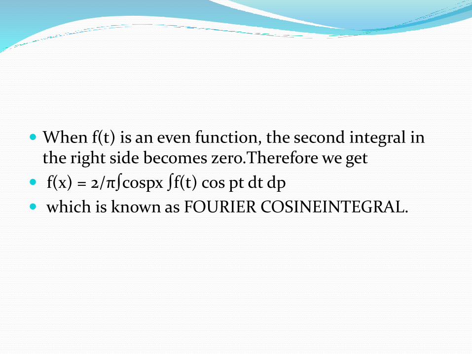
When f(t) is an even function, the second integral in the right side becomes zero.Therefore we get
f(x) = 2/π∫cospx ∫f(t) cos pt dt dp
which is known as FOURIER COSINEINTEGRAL.

FOURIER INTEGRAL IN COMPLEX FORM Since cos p(t-x) is an even functionof p, we have
f(x) = 1/2π∫∫eip(t-x) f(t) dt dp
which is the required complex form.

INFINITE FOURIER TRANSFORM The fourier transform of a function f(x) is given by
F{f(x)} = F(p) = ∫f(x) eipx dx
The inverse fourier transform of F(p) is given by
f(x) = 1/2π ∫ F (p) e-ipx dp

FOURIER SINE TRANSFORM The finite Fourier sine transform of f(x) when 0<x<l, is
definedas
Fs{f(x) = Fs (n) sin (nπx)/l dx where n is an integer and the function f(x) is given by
f(x) = 2/l∑ Fs (n) sin (nπx)/l is called the Inverse finite Fourier sine transform Fs(n)

FOURIER COSINE TRANSFORM We have f(x) = 2/π∫cospx ∫f(t) cos pt dt dp
Which is the fourier cosine integral .Now
Fc(p) = ∫ f(x) cos px dx then
f(x) becomes f(x) =2/π∫ Fc(p) cos px dp which is the fourier cosine transform.
PROPERTIES Linear property of Fourier transform
Change of Scale property
Shifting property
Modulation property

Interpolation and Curve Fitting
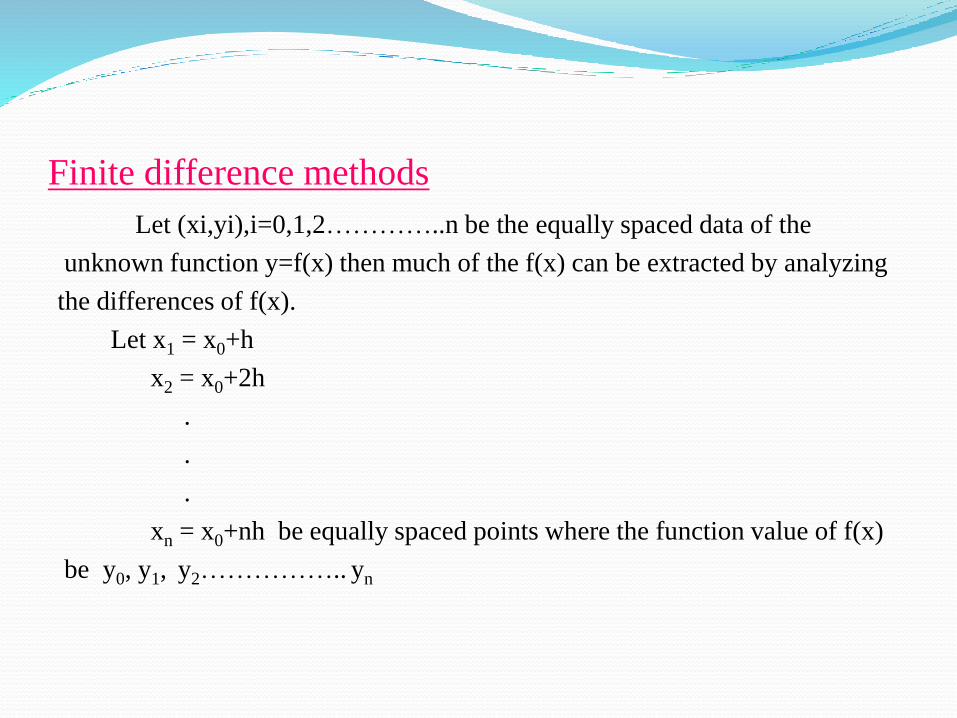
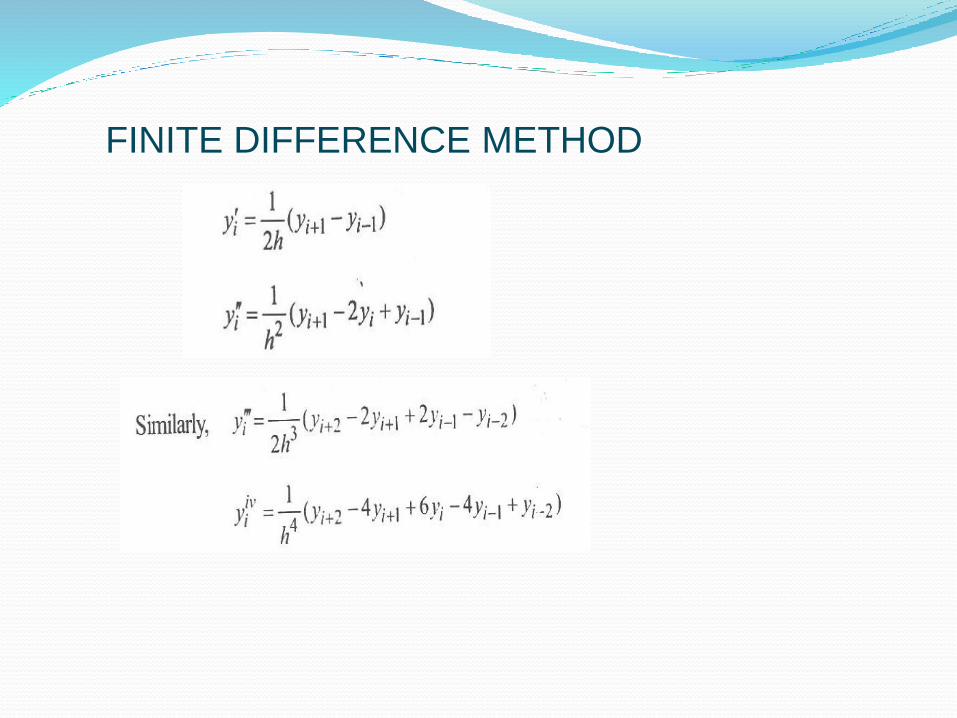
Finite difference methods
Let (xi,yi),i=0,1,2…………..n be the equally spaced data of the
unknown function y=f(x) then much of the f(x) can be extracted by analyzing
the differences of f(x).
Let x1 = x0+h
x2 = x0+2h
.
.
.
xn = x0+nh be equally spaced points where the function value of f(x)
be y0, y1, y2…………….. yn
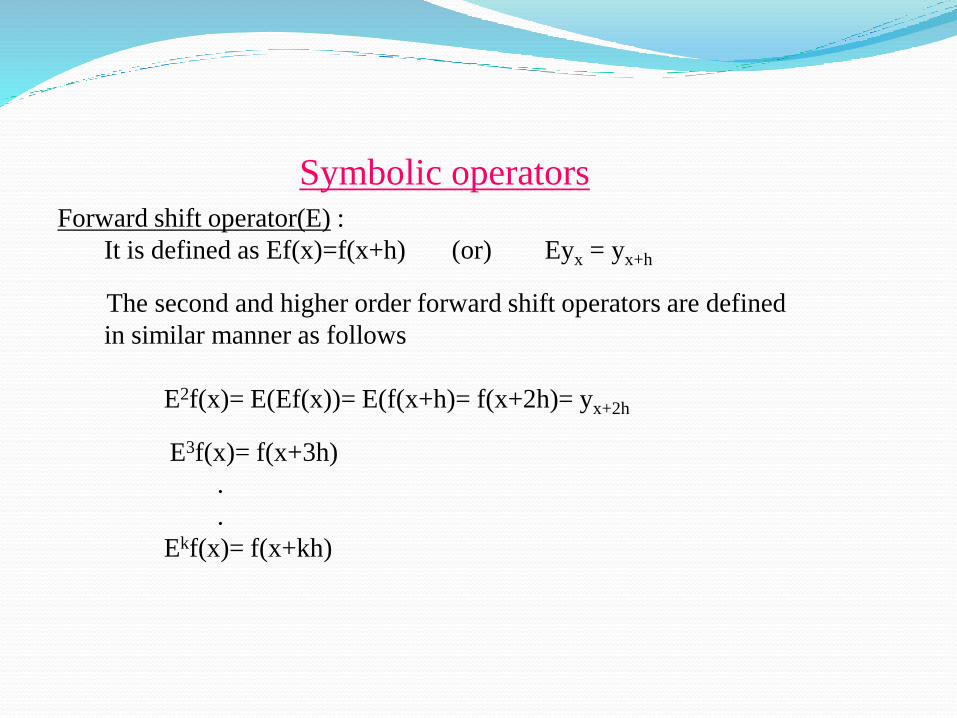
Symbolic operatorsForward shift operator(E) :
It is defined as Ef(x)=f(x+h) (or) Eyx = yx+h
The second and higher order forward shift operators are defined
in similar manner as follows
E2f(x)= E(Ef(x))= E(f(x+h)= f(x+2h)= yx+2h
E3f(x)= f(x+3h)
.
.
Ekf(x)= f(x+kh)
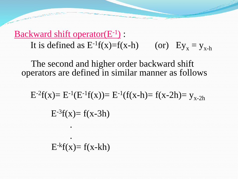
Backward shift operator(E-1) :
It is defined as E-1f(x)=f(x-h) (or) Eyx = yx-h
The second and higher order backward shift operators are defined in similar manner as follows
E-2f(x)= E-1(E-1f(x))= E-1(f(x-h)= f(x-2h)= yx-2h
E-3f(x)= f(x-3h)
.
.
E-kf(x)= f(x-kh)

Forward difference operator (∆) :
The first order forward difference operator of a function f(x) with increment h in x is given by
∆f(x)=f(x+h)-f(x) (or) ∆fk =fk+1-fk ; k=0,1,2………
∆2f(x)= ∆[∆f(x)]= ∆[f(x+h)-f(x)]= ∆fk+1- ∆fk ; k=0,1,2…………
…………………………….
…………………………….
Relation between E and ∆ :
∆f(x)=f(x+h)-f(x)
=Ef(x)-f(x) [Ef(x)=f(x+h)]
=(E-1)f(x)
∆=E-1 E=1+ ∆
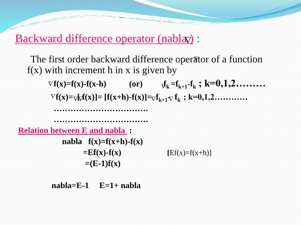
Backward difference operator (nabla ) :
The first order backward difference operator of a function f(x) with increment h in x is given by
f(x)=f(x)-f(x-h) (or) fk =fk+1-fk ; k=0,1,2………
f(x)= [ f(x)]= [f(x+h)-f(x)]= fk+1- fk ; k=0,1,2…………
…………………………….
…………………………….
Relation between E and nabla :
nabla f(x)=f(x+h)-f(x)
=Ef(x)-f(x) [Ef(x)=f(x+h)]
=(E-1)f(x)
nabla=E-1 E=1+ nabla

Central difference operator ( δ) :
The central difference operator is defined as
δf(x)= f(x+h/2)-f(x-h/2)
δf(x)= E1/2f(x)-E-1/2f(x)
= [E1/2-E-1/2]f(x)
δ= E1/2-E-1/2
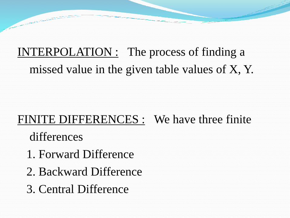
INTERPOLATION : The process of finding a
missed value in the given table values of X, Y.
FINITE DIFFERENCES : We have three finite
differences
1. Forward Difference
2. Backward Difference
3. Central Difference

RELATIONS BETWEEN THE OPERATORS
IDENTITIES:
1. ∆=E-1 or E=1+ ∆
2. = 1- E -1
3. δ = E 1/2 – E -1/2
4. µ= ½ (E1/2-E-1/2)
5. ∆=E = E= δE1/2
6. (1+ ∆)(1- )=1
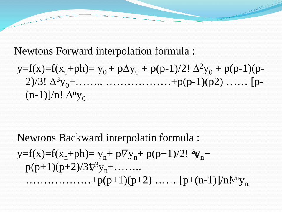
Newtons Forward interpolation formula :
y=f(x)=f(x0+ph)= y0 + p∆y0 + p(p-1)/2! ∆2y0 + p(p-1)(p-
2)/3! ∆3y0+…….. ………………+p(p-1)(p2) …… [p-
(n-1)]/n! ∆ny0 .
Newtons Backward interpolatin formula :
y=f(x)=f(xn+ph)= yn+ p𝛻yn+ p(p+1)/2! 2yn+
p(p+1)(p+2)/3! 3yn+……..
………………+p(p+1)(p+2) …… [p+(n-1)]/n! nyn.
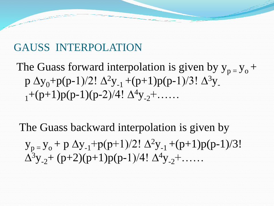
GAUSS INTERPOLATION
The Guass forward interpolation is given by yp = yo +
p ∆y0+p(p-1)/2! ∆2y-1 +(p+1)p(p-1)/3! ∆3y-
1+(p+1)p(p-1)(p-2)/4! ∆4y-2+……
The Guass backward interpolation is given by
yp = yo + p ∆y-1+p(p+1)/2! ∆2y-1 +(p+1)p(p-1)/3!
∆3y-2+ (p+2)(p+1)p(p-1)/4! ∆4y-2+……
INTERPOLATIN WITH UNEQUAL INTERVALS:
The various interpolation formulae Newton’s forward
formula, Newton’s backward formula possess can be
applied only to equal spaced values of argument. It is
therefore, desirable to develop interpolation formula for
unequally spaced values of x. We use Lagrange’s
interpolation formula.
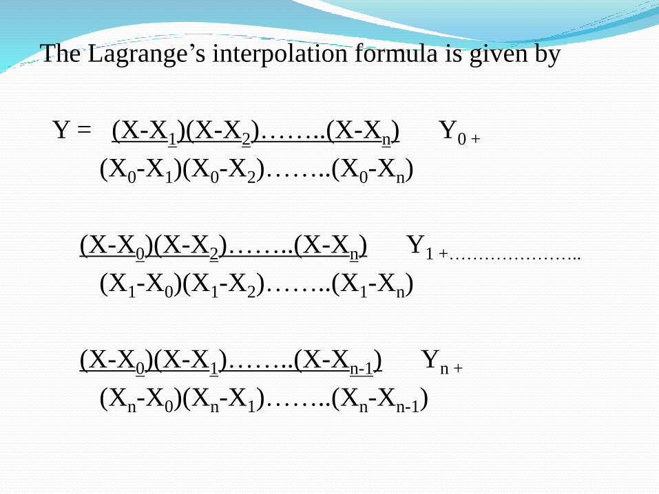
The Lagrange’s interpolation formula is given by
Y = (X-X1)(X-X2)……..(X-Xn) Y0 +
(X0-X1)(X0-X2)……..(X0-Xn)
(X-X0)(X-X2)……..(X-Xn) Y1 +…………………..
(X1-X0)(X1-X2)……..(X1-Xn)
(X-X0)(X-X1)……..(X-Xn-1) Yn +
(Xn-X0)(Xn-X1)……..(Xn-Xn-1)

CURVE FITTING

INTRODUCTION : In interpolation, We have seen that when exact values of the function Y=f(x) is given we fit the function using various interpolation formulae. But sometimes the values of the function may not be given. In such cases, the values of the required function may be taken experimentally. Generally these expt. Values contain some errors. Hence by using these experimental values . We can fit a curve just approximately which is known as approximating curve.
Now our aim is to find this approximating curve as much
best as through minimizing errors of experimental values
this is called best fit otherwise it is a bad fit.
In brief by using experimental values the process of
establishing a mathematical relationship between two
variables is called CURVE FITTING.

METHOD OF LEAST SQUARES
Let y1, y2, y3 ….yn be the experimental values of
f(x1),f(x2),…..f(x n) be the exact values of the function
y=f(x). Corresponding to the values of x=xo,x1,x2….x n
.Now error=experimental values –exact value. If we
denote the corresponding errors of y1, y2,….yn as
e1,e2,e3,…..en , then e1=y1-f(x1), e2=y2-f(x2 )

e3=y3-f(x3)…….en=yn-f(xn).These errors e1,e2,e3,……en,may be either positive or negative.For our convenient to make all errors into +ve to the square of errors i.e e1
2,e22,……en
2.In order to obtain the best fit of curve we have to make the sum of the squares of the errors as much minimum i.e e1
2+e22+……+en
2 is minimum.
METHOD OF LEAST SQUARES Let S=e1
2+e22+……+en
2, S is minimum.When S becomes
as much as minimum.Then we obtain a best fitting of a
curve to the given data, now to make S minimum we have
to determine the coefficients involving in the curve, so
that S minimum.It will be possible when differentiating S
with respect to the coefficients involving in the curve and
equating to zero.
FITTING OF STRAIGHT LINE
Let y = a + bx be a straight line
By using the principle of least squares for solving the
straight line equations.
The normal equations are
∑ y = na + b ∑ x
∑ xy = a ∑ x + b ∑ x2
solving these two normal equations we get the values
of a & b ,substituting these values in the given straight
line equation which gives the best fit.
FITTING OF PARABOLALet y = a + bx + cx2 be the parabola or second degree
polynomial.
By using the principle of least squares for solving the parabola
The normal equations are
∑ y = na + b ∑ x + c ∑ x2
∑ xy = a ∑ x + b∑ x2 + c ∑ x3
∑ x2y = a ∑ x2 + b ∑ x3 + c ∑ x4
solving these normal equations we get the values of a,b& c, substituting these values in the given parabola which gives the best fit.

FITTING OF AN
EXPONENTIAL CURVE
The exponential curve of the form
y = a ebx
taking log on both sides we get
logey = logea + logeebx
logey = logea + bx logee
logey = logea + bx
Y = A+ bx
Where Y = logey, A= logea
This is in the form of straight line equation and this can
be solved by using the straight line normal equations we
get the values of A & b, for a =eA, substituting the values
of a & b in the given curve which gives the best fit.
EXPONENTIAL CURVEThe equation of the exponential form is of the form y =
abx
taking log on both sides we get
log ey = log ea +log ebx
Y = A + Bx
where Y= logey, A= logea , B= logeb
this is in the form of the straight line equation which can be solved by using the normal equations we get the values of A & B for a = eA
b = eB substituting these values in the equation which gives the best fit.
FITTING OF POWER CURVE
Let the equation of the power curve be
y = a xb
taking log on both sides we get
log ey = logea + log exb
Y = A + Bx
this is in the form of the straight line equation which can be solved by using the normal equations we get the values of A & B, for a = eA b= eB, substituting these values in the given equation which gives the best fit.

Solutions of Algebraic and Transcendental equations and
Linear system of equations

Method 1: Bisection method
If a function f(x) is continuous b/w x0 and x1 and f(x0) & f(x1) are of opposite signs, then there exsist at least one root b/w x0 and x1
Let f(x0) be –ve and f(x1) be +ve ,then the root lies b/w xo
and x1 and its approximate value is given by x2=(x0+x1)/2
If f(x2)=0,we conclude that x2 is a root of the equ f(x)=0
Otherwise the root lies either b/w x2 and x1 (or) b/w x2 and x0
depending on wheather f(x2) is +ve or –ve
Then as before, we bisect the interval and repeat the process untill the root is known to the desired accuracy
Method 2: Iteration method or successive approximation
Consider the equation f(x)=0 which can take in the form
x = ø(x) -------------(1)
where |ø1(x)|<1 for all values of x.
Taking initial approximation is x0we put x1=ø(x0) and take x1 is the first approximation
x2=ø(x1) , x2 is the second approximation
x3=ø(x2) ,x3 is the third approximation
.
.
xn=ø(xn-1) ,xn is the nth approximation
Such a process is called an iteration process
Method 3: Newton-Raphson method or Newton iteration method
Let the given equation be f(x)=0
Find f1(x) and initial approximation x0
The first approximation is x1= x0-f(x0)/ f1(x0)
The second approximation is x2= x1-f(x1)/ f1(x1)
.
.
The nth approximation is xn= xn-1-f(xn)/ f1(xn)
11 1 12 2 13 3 1
21 1 22 2 23 3 2
31 1 32 2 33 3 3
a x a x a x b
a x a x a x b
a x a x a x b
11 12 13 1 1
21 22 23 2 2
31 32 33 3 3
, ,
a a a x b
A a a a X x B b
a a a x b
11 11 12 13
21 22 22 23
31 32 33 33
0 0
0 , 0
0 0
l u u u
L l l U u u
l l l u
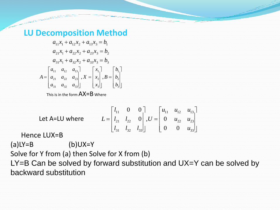
LU Decomposition Method
This is in the form AX=B Where
Let A=LU where
Hence LUX=B (a)LY=B (b)UX=YSolve for Y from (a) then Solve for X from (b)LY=B Can be solved by forward substitution and UX=Y can be solved by
backward substitution
1 1 1 1
2 2 2 2
3 3 3 3
a x b y c z d
a x b y c z d
a x b y c z d
1 1 1 1 1 1
1
2 2 2 2 2 2
2
3 3 3 3 3 3
3
1[ ]
1[ ]
1[ ]
x d b y c z k l y m za
y d a x c z k l x m zb
z d a x b y k l x m yc
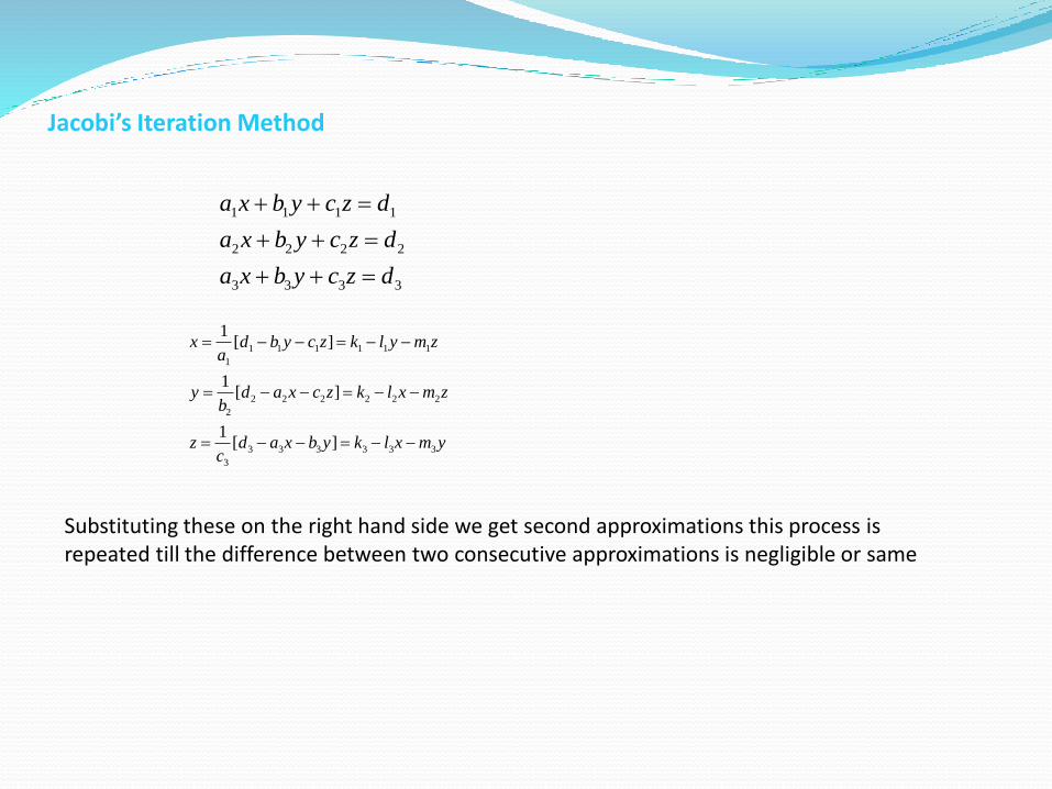
Jacobi’s Iteration Method
Substituting these on the right hand side we get second approximations this process is repeated till the difference between two consecutive approximations is negligible or same

Gauss-Seidel iteration Method
1 1 1 1
2 2 2 2
3 3 3 3
a x b y c z d
a x b y c z d
a x b y c z d
1 1 1 1 1 1
1
2 2 2 2 2 2
2
3 3 3 3 3 3
3
1[ ]
1[ ]
1[ ]
x d b y c z k l y m za
y d a x c z k l x m zb
z d a x b y k l x m yc
as soon as new approximation for an unknown is found it is immediately
used in the next step

Numerical Integration and Numerical solution of First order differential equations
NUMERICAL INTEGRATION Numerical Integration is a process of finding the value
of a definite integral.When a function y = f(x) is not known explicity. But we give only a set of values of the function y = f(x) corresponding to the same values of x. This process when applied to a function of a single variable is known as a quadrature.

NUMERICAL INTEGRATION For evaluating the Numerical Integration we have
three important rules i.e
Trapezoidal Rule
Simpsons 1\3 Rule
Simpsons 3\8 th Rule
NUMERICAL INTEGRATION
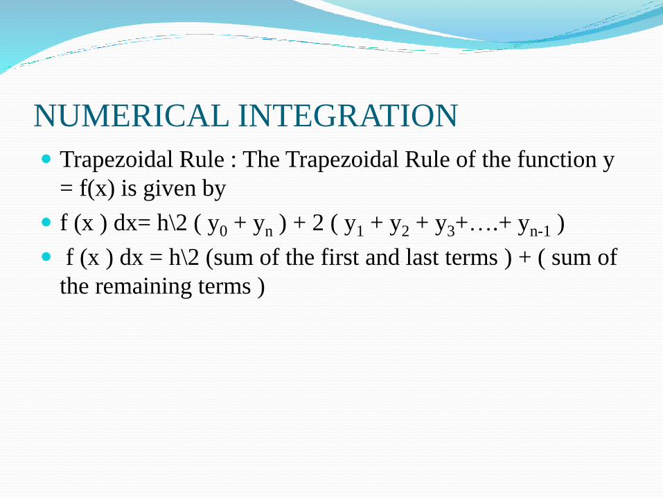
Trapezoidal Rule : The Trapezoidal Rule of the function y
= f(x) is given by
f (x ) dx= h\2 ( y0 + yn ) + 2 ( y1 + y2 + y3+….+ yn-1 )
f (x ) dx = h\2 (sum of the first and last terms ) + ( sum of
the remaining terms )
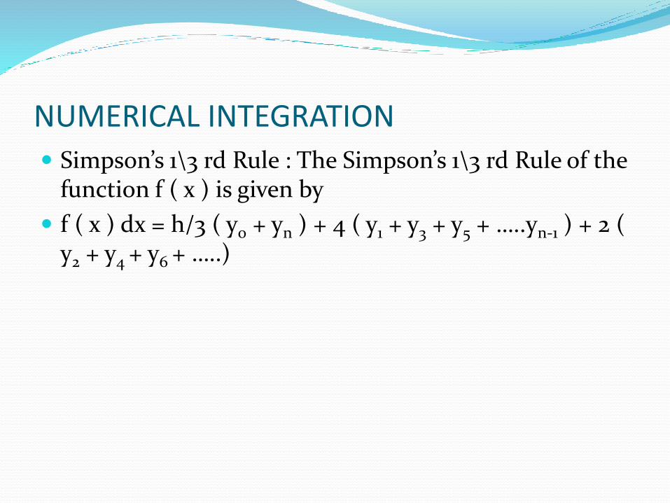
NUMERICAL INTEGRATION Simpson’s 1\3 rd Rule : The Simpson’s 1\3 rd Rule of the
function f ( x ) is given by
f ( x ) dx = h/3 ( y0 + yn ) + 4 ( y1 + y3 + y5 + …..yn-1 ) + 2 ( y2 + y4 + y6 + …..)

NUMERICAL INTEGRATION Simpson’s 3/8 th Rule : The Simpson’s 3/8 th rule for
the function f ( x ) isgiven by
f ( x ) dx = 3h/8 ( y0 + yn ) + 2 ( y3 + y6 + y9 + ……) + 3 ( y1
+ y2 +y4 +……)
f (x ) dx = 3h/8 ( sum of the first and the last term) + 2 ( multiples of three ) + 3 ( sum of the remaining terms )
INTRODUCTION There exists large number of ordinary differential
equations, whose solution cannot be obtained by the known analytical methods. In such cases, we use numerical methods to get an approximate solution o f a given differential equation with given initial condition.

NUMERICAL DIFFERIATION Consider an ordinary differential equation of first
order and first degree of the form
dy/dx = f ( x,y ) ………(1)
with the intial condition y (x0 ) = y0 which is called initial value problem.
T0 find the solution of the initial value problem of the form (1) by numerical methods, we divide the interval (a,b) on whcich the solution is derived in finite number of sub- intervals by the points
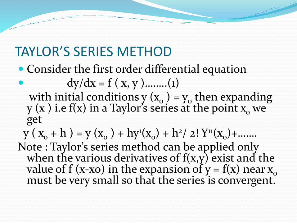
TAYLOR’S SERIES METHOD Consider the first order differential equation dy/dx = f ( x, y )……..(1)
with initial conditions y (xo ) = y0 then expanding y (x ) i.e f(x) in a Taylor’s series at the point xo we get
y ( xo + h ) = y (x0 ) + hy1(x0) + h2/ 2! Y11(x0)+…….Note : Taylor’s series method can be applied only
when the various derivatives of f(x,y) exist and the value of f (x-x0) in the expansion of y = f(x) near x0must be very small so that the series is convergent.

PICARDS METHOD OF SUCCESSIVE APPROXIMATION Consider the differential equation
dy/dx = f (x,y) with intial conditions
y(x0) = y0 then
The first approximation y1 is obtained by
y1 = y0 + f( x,y0 ) dx
The second approximation y2 is obtained by y2 = y1 + f (x,y1 ) dx
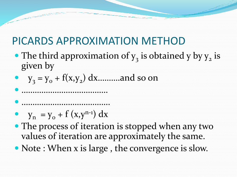
PICARDS APPROXIMATION METHOD The third approximation of y3 is obtained y by y2 is
given by
y3 = y0 + f(x,y2) dx……….and so on
…………………………………
………………………………….
yn = y0 + f (x,yn-1) dx
The process of iteration is stopped when any two values of iteration are approximately the same.
Note : When x is large , the convergence is slow.

EULER’S METHOD Consider the differential equation
dy/dx = f(x,y)………..(1)
With the initial conditions y(x0) = y0
The first approximation of y1 is given by
y1 = y0 +h f (x0,,y0 )
The second approximation of y2 is given by
y2 = y1 + h f ( x0 + h,y1)

EULER’S METHOD
The third approximation of y3 is given by
y3 = y2 + h f ( x0 + 2h,y2 )
………………………………
……………………………..
……………………………...
yn = yn-1 + h f [ x0 + (n-1)h,yn-1 ]
This is Eulers method to find an appproximate solution of the given differential equation.

IMPORTANT NOTE Note : In Euler’s method, we approximate the curve of
solution by the tangent in each interval i.e by a sequence of short lines. Unless h is small there will be large error in yn . The sequence of lines may also deviate considerably from the curve of solution. The process is very slow and the value of h must be smaller to obtain accuracy reasonably.
MODIFIED EULER’S METHOD By using Euler’s method, first we have to find the value
of y1 = y0 + hf(x0 , y0)
WORKING RULE
Modified Euler’s formula is given by
yik+1 = yk + h/2 [ f(xk ,yk) + f(xk+1,yk+1
when i=1,y(0)k+1 can be calculated
from Euler’s method.
MODIFIED EULER’S METHOD When k=o,1,2,3,……..gives number of iterations
i = 1,2,3,…….gives number of times a particular iteration k is repeated when
i=1
Y1k+1= yk + h/2 [ f(xk,yk) + f(xk+1,y k+1)],,,,,,
RUNGE-KUTTA METHODThe basic advantage of using the Taylor series
method lies in the calculation of higher order total derivatives of y. Euler’s method requires the smallness of h for attaining reasonable accuracy. In order to overcomes these disadvantages, the Runge-Kutta methods are designed to obtain greater accuracy and at the same time to avoid the need for calculating higher order derivatives.The advantage of these methods is that the functional values only required at some selected points on the subinterval.
R-K METHOD Consider the differential equation
dy/dx = f ( x, y )
With the initial conditions y (xo) = y0
First order R-K method :
y1= y (x0 + h )
Expanding by Taylor’s series
y1 = y0 +h y10 + h2/2 y11
0 +…….
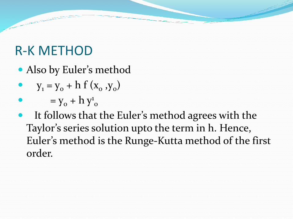
R-K METHOD Also by Euler’s method
y1 = y0 + h f (x0 ,y0)
= y0 + h y10
It follows that the Euler’s method agrees with the Taylor’s series solution upto the term in h. Hence, Euler’s method is the Runge-Kutta method of the first order.

The second order R-K method is given by
y1= y0 + ½ ( k1 + k2 )
where k1 = h f ( x0,, y0 )
k2 = h f (x0 + h ,y0 + k1 )
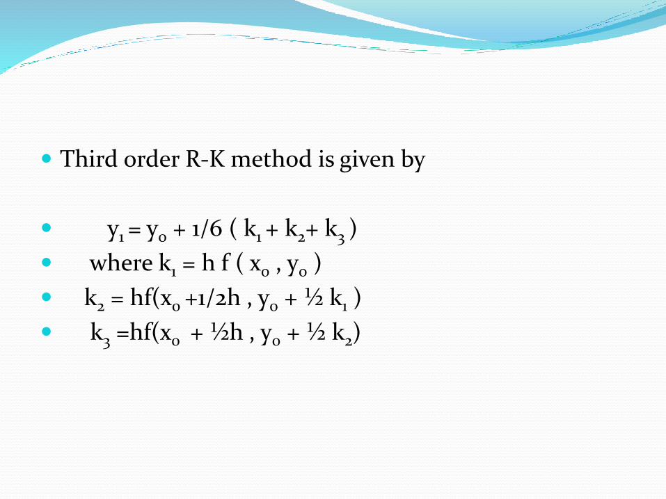
Third order R-K method is given by
y1 = y0 + 1/6 ( k1 + k2+ k3 )
where k1 = h f ( x0 , y0 )
k2 = hf(x0 +1/2h , y0 + ½ k1 )
k3 =hf(x0 + ½h , y0 + ½ k2)

The Fourth order R – K method :
This method is most commonly used and is often referred to as Runge – Kutta method only. Proceeding as mentioned above with local discretisation error in this method being O (h5), the increment K of y correspoding to an increment h of x by Runge – Kutta method from
dy/dx = f(x,y),y(x0)=Y0 is given by
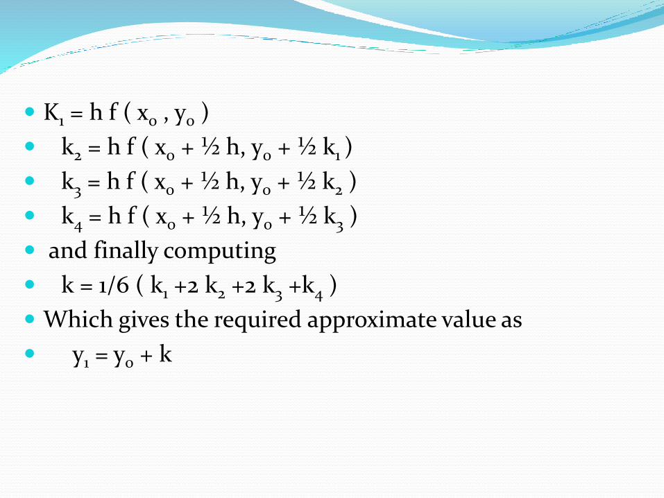
K1 = h f ( x0 , y0 )
k2 = h f ( x0 + ½ h, y0 + ½ k1 )
k3 = h f ( x0 + ½ h, y0 + ½ k2 )
k4 = h f ( x0 + ½ h, y0 + ½ k3 )
and finally computing
k = 1/6 ( k1 +2 k2 +2 k3 +k4 )
Which gives the required approximate value as
y1 = y0 + k
R-K METHODNote 1 : k is known as weighted mean of
k1, k2, k3 and k4.
Note 2 : The advantage of these methods is that the operation is identical whether the differential equation is linear or non-linear.
FINITE DIFFERENCE METHOD

Characteristic matrix: Let A be a square matrix of order n then
the matrix (A-λI) is called Characteristic matrix of A.where I
is the unit matrix of order n and λ is any scalar
Ex: Let A= then
A- λI= is the characteristic matrix of A
Characteristic polynomial: Let A be square matrix of order n then | A- λI| is
called characteristic polynomial of A
Ex: Let A=
then | A- λI| = λ2-2λ+9 is the characteristic polynomial of A
43
21
43
21
14
21

Characteristic equation: Let A be square matrix of order n then
| A- λI|=0 is called characteristic equation of A
Ex: Let A=
then | A- λI| = λ2-2λ+9=0 is the characteristic equation of A
Eigen values: The roots of the characteristic equation | A- λI|=0 are
called the eigen values
Ex: Let A= then | A- λI|=λ2-6λ+5=0
Therefore λ=1,5 are the eigen values of the matrix A
14
21
43
12
Eigen vector: If λ is an eigen value of the square matrix A. If there exists a non- zero vector X such that AX=λX is said to be eigen vector corresponding to eigen value λ of a square matrix A
Eigen vector must be a non-zero vector
If λ is an eigen value of matrix A if and only if there exists a non-zero vector X such that AX=λX
I f X is an eigen vector of a matrix A corresponding to the eigenvalue λ, then kX is also an eigen vector of A corresponding to the same eigen vector λ. K is a non zero scalar.

Properties of eigen values and eigen vectors
The matrices A and AT have the same eigen values.
If λ1, λ2,…..λn are the eigen values of A then
1/ λ1, 1/λ2 ……1/λn are the eigen values of A-1.
If λ1, λ2,…..λn are the eigen values of A then λ1k, λ2
k,…..λnk are
the eigen values of Ak.
If λ is the eigen value of a non singular matrix A, then |A|/λ is
the eigen value of A.

The sum of the eigen values of a matrix is the trace of
the matrix
If λ is the eigen value of A then the eigen values of
B= aoA2+ a1A+a2I is aoλ2+a1λ+a2.
Similar Matrices : Two matrices A&B are said to be
similar if their exists an invertable matrix P such
that B=P-1AP.
Eigen values of two similar matrices are same
If A & B are square matrices and if A is invertable then the matrices A-1B & BA-1 have the same eigen values

Power method for finding eigenvalues
1. Start with an initial guess for x
2. Calculate w = Ax
3. Largest value (magnitude) in w is the
estimate of eigenvalue
4. Get next x by rescaling w (to avoid
the computation of very large matrix
An )
5. Continue until converged
Power Method

Start with initial guess z = x0
Power Method
Azwz
w Azw
Azwz
w Azw
)2(
k
)2(
)2(
k
)2()3(
)2(
k
)2(
k
)2()2(
)1(
k
)1(
)1(
k
)1()2(
)1(
k
)1(
k
)1()1(
k
n
kkk
n thenIf
321
321 ,
rescaling
k is the
dominant
eigenvalue

Power Method
(1)
0
(1) (1) (2)
(2) (2) (3)
( ) ( ) ( 1)
1. 1,1,...,1
2. ;
3. ;
...
T
k
k
k k k
normalize
n
Initial guess z x
Calculate Az w z z by biggest w
Calculate Az w z z by biggest w
Calculate
ormalize
Az w z
For large number of iterations, should converge to the largest eigenvalue
The normalization make the right hand side converge to , rather than n


![instructor.sdu.edu.kzinstructor.sdu.edu.kz/~merey/[Kreyszig_E.]_Advanced_engineering... · ERWIN KREYSZIG ADVANCED ENGINEERING TH EDITION MATHEMATICS WILEY INTERNATIONAL DITION RESTRICTED!](https://static.fdocuments.net/doc/165x107/5e8ca70682c48e37925657d3/mereykreyszigeadvancedengineering-erwin-kreyszig-advanced-engineering.jpg)